Hexapod
Robot













Dalhousie
Mechanical
Engineering


Senior
Year
Design
Team
2








To


Dalhousie
University


Mechanical
Engineering
Department














December
1,
2008

Rene
d’Entremont

Brett
MacDonald

Leslie
Ssebazza

Seth
Stoddart

ii





Abstract


The
Hexapod
Walking
Robot
designed
by
Group#2
is
in
the
end
stages
of
design.
A
final
iteration


of
chassis
and
leg
design
has
been
selected,
and
is
such
that
walking
speed
is
maximized.
Prior


designs
 have
 been
 discarded
 based
 on
 complexity
 or
 physical
 motion
 limitations.
 Prototypes


have
been
both
physically
and
virtually
(Matlab
Simulink)
constructed
with
success
in
order
to


demonstrate
proof
of
concept.
Current
programming
is
able
to
produce
a
single
step,
using
the


desired
tripod
gait,
for
one
leg
only.
This
program
has
been
used
to
make
the
physical
prototype


move
in
the
stepping
motion.
The
basic
positioning
code
has
been
written
and
is
ready
to
enter


the
motion
planning
stage.
Aspects
of
the
project
still
to
be
completed
include
manufacturing


and
 assembly
 as
 well
 as
 communication
 between
 the
 full
 driving
 programs
 and
 the
 Hexapod.


These


will


be


finished


in


the


coming


term.


iii








Table
of
Contents


Abstract........................................................................................................................................... ii


Table
of
Contents............................................................................................................................iii


List
of
Figures ..................................................................................................................................vi


List
of
Tables ...................................................................................................................................vi


1


Introduction ............................................................................................................................ 1


1.1


Background...................................................................................................................... 1


1.2


Project
Description .......................................................................................................... 1


2


Design
Requirements.............................................................................................................. 3


2.1


Primary ............................................................................................................................ 3


2.1.1


Design...................................................................................................................... 3


2.1.2


Mobility................................................................................................................... 3


2.2


Secondary ........................................................................................................................ 4


3


Design
Alternatives ................................................................................................................. 5


3.1


Alternative
1:
Mobility
‐
Spider,
Outboard
Rotate .......................................................... 5


3.2


Alternative
2:
Smooth‐
Central
Suspension
Pivot............................................................ 5


3.3


Alternative
3:
Fast‐
Central
Rotation,
No
Suspension ..................................................... 6


3.4


Design
Selection .............................................................................................................. 7


4


Design
Refinements ................................................................................................................ 9


4.1


Securing
Servo
Motors .................................................................................................... 9


4.2


Suspension
and
Grip...................................................................................................... 10


4.3


Rapid
Prototype............................................................................................................. 11


5


Final
Design........................................................................................................................... 12


5.1


Overview........................................................................................................................ 12


5.2


Frame............................................................................................................................. 12


5.2.1


Description............................................................................................................ 12


5.2.2


Fabrication ............................................................................................................ 13


5.2.3


To
Be
Determined ................................................................................................. 13


5.3


Legs................................................................................................................................ 13


iv





5.3.1


Description............................................................................................................ 13


5.3.2


Fabrication ............................................................................................................ 15


5.3.3


To
Be
Determined .....................................................Error!
Bookmark
not
defined.


5.4


Control
Hardware .......................................................................................................... 15


5.4.1


Description............................................................................................................ 15


5.4.2


Fabrication ............................................................................................................ 16


5.4.3


To
Be
Determined ................................................................................................. 16


5.5


Control
Software ........................................................................................................... 16


5.5.1


Motion
Planning.................................................................................................... 16


5.5.2


Conversion ............................................................................................................ 17


5.5.3


Communication..................................................................................................... 18


6


Testing................................................................................................................................... 19


6.1


Finite
Element
Analysis
(FEA) ........................................................................................ 19


6.1.1


Model
Description................................................................................................. 19


6.1.2


Results................................................................................................................... 19


6.2


Hexapod
Motion
Simulations ........................................................................................ 20


6.2.1


Simulink................................................................................................................. 20


6.2.2


Virtual
Reality
Toolbox.......................................................................................... 21


6.3


Working
Leg................................................................................................................... 22


6.3.1


Mechanical............................................................................................................ 22


6.3.2


Hardware .............................................................................................................. 22


6.3.3


Software................................................................................................................ 22


7


Project
Status........................................................................................................................ 24


7.1


Progress......................................................................................................................... 24


7.2


Technician
Time............................................................................................................. 24


8


Budget................................................................................................................................... 25


9


Conclusion
and
Recommendations....................................................................................... 27


Appendix
A:
2
DOF
Inverse
Kinematic
MATLAB
program ............................................................. 28


Appendix
B:
Angles
to
Registry
Format
Converter
Code .............................................................. 30


Appendix
C:
Winter
Term
Gantt
Chart.......................................................................................... 31


Appendix
D:
Simulink
Gait ............................................................................................................ 33


Appendix
E:
Fabrication
Drawings ................................................................................................ 35


v








vi








List
of
Figures


F

IGURE


1:




O

UTBOARD


M

OUNTED


L

EG


A

SSEMBLY

...................................................................................................... 5




F

IGURE


2:




C

ENTRAL


P

IVOTING


L

EGS


A

SSEMBLY

......................................................................................................... 5




F

IGURE


3:




L

EG
OF
THE


I

NBOARD


M

OUNTED


C

ONFIGURATION

...................................................................................... 6




F

IGURE


4:




I

NBOARD


M

OUNTED


L

EG


A

SSEMBLY

......................................................................................................... 7




F

IGURE


5:




S

ELECTED


D

ESIGN
WITH
LEG
AND
BODY
WEIGHT
CONSIDERATIONS

.................................................................. 9




F

IGURE


6:




R

EFINED


L

EG


A

SSEMBLY

,


USING
ALL
FOUR
BOLT
HOLES

. .............................................................................. 10




F

IGURE


7:




S

PRING
RATED


S

HOCK
ABSORBERS


(

HTTP

://

WWW

.

MCMASTER

.

COM

/

CATALOG

/114/

GFX

/

LARGE

/3740

KC

1

L

.

GIF

). 10




F

IGURE


8:




N

EOPRENE


B

UMPER


(

HTTP

://

WWW

.

MCMASTER

.

COM

) .............................................................................. 11




F

IGURE


9




:




F

INAL


D

ESIGN
OF


H

EXAPOD


R

OBOT

....................................................................................................... 12




F

IGURE


10




:




B

OTTOM


V

IEW
OF


F

RAME


A

SSEMBLY

................................................................................................... 13




F

IGURE


11




:




L

EG


A

SSEMBLY

................................................................................................................................. 14




F

IGURE


12




:




T

HREE


L

EG


S

ECTIONS

,


NAMED
AS
THE


“F

IRST

,




S

ECOND
AND


T

HIRD
LEG
SECTIONS

”




(

LEFT
TO
RIGHT

).................. 15




F

IGURE


13:




V

ON

‐M

ISES


S

TRESS
OF
THE


F

IRST


B

AR


L

INKAGE

...................................................................................... 20




F

IGURE


14:




B

LOCK


D

IAGRAM
REPRESENTATION
OF
A
DIFFERENTIAL
MECHANICAL
SYSTEM

................................................ 21




List
of
Tables


T

ABLE


1:





W

EIGHTED


C

OMPARISON


T

ABLE

............................................................................................................... 7




T

ABLE


2:




S

ERVO


S

PECIFICATIONS


S

UMMARY

............................................................................................................. 8




T

ABLE


3:




E

STIMATED


M

ACHINING


T

IME


R

EQUIRED
FROM


D

EPARTMENT

...................................................................... 24




T

ABLE


4:




P

ROPOSED


B

UDGET

.............................................................................................................................. 25




1





1 Introduction





1.1 Background


The
Hexapod
Remotely
Operated
Vehicle
(ROV)
was
first
proposed
as
a
project
by
Dr.
Pan


of
Dalhousie
University
as
an
idea
for
the
Mechanical
Engineering
Senior
Design
Project.


The
idea
of
building
robots
and
ROVs
for
design
project
is
not
new,
as
tracked,
wheeled,


and
water
based
ROVs
have
all
been
produced
in
the
past,
but
leg
based
ROVs
have
yet
to


be
 attempted.
 The
 challenges
 are
 obvious
 as
 walking
 is
 a
 complicated
 method
 of


travelling
 that
 required
 a
 complex
 control
 system
 to
 coordinate
 the
 movements.


However,
 the
 benefits
 are
 numerous.
 Legs
 offer
 more
 freedom
 of
 movement
 to
 the


chassis
of
the
ROV;
it
may
level
itself
on
uneven
terrain,
tackle
obstacles
that
wheels
(of
a


proportionate
size)
may
not,
and
move
in
all
directions
without
changing
the
orientation


of
the
body.
Legs
can
also
be
used
to
manipulate
objects
with
some
precision
or
adjust


the
height
of
the
body
for
increased
stability
or
travel
into
restricted
spaces.
Overall,
the


freedom
of
motion
provided
by
legs
is
extremely
useful,
with
few
drawbacks
(beyond
the


complex
programming).
One
such
drawback
is
the
low
forward
speed
that
most
walking


robots
are
able
to
accomplish.
The
group
has
identified
this
as
a
challenge
and
an
area
for


improvement
 over
 traditional
 hexapod
 designs.
 The
 project
 will
 be
 unique
 from
 other


hexapods
 since
 it
 is
 intended
 to
 be
 a
 platform
 onto
 which
 additional
 sensors
 can
 be


mounted,
making
it
capable
of
doing
many
different
tasks.
In
comparison,
other
hexapods


tend
to
be
simply
a
body
and
legs
and
are
designed
onto
to
move
around.
The
group
will


design
 a
 chassis
 and
 legs,
 and
 initial
 and
 final
 control
 systems.
 The
 intent
 is
 that
 the


finished
product
be
mechanically
capable
and
upgrade
friendly,
so
future
iterations
can


accomplish
increasingly
complex
tasks
and
motions.


1.2 Project
Description


The
ROV
will
have
18
degrees
of
freedom
(DOF)
as
stated
in
the
design
requirements.
To


be
as
mechanically
sound
as
possible,
the
robot
will
use
a
modular
design,
where
a
small


list
of
spare
parts
may
be
kept
on
hand
to
repair
the
robot
in
the
case
of
failure.
These


parts
may
be
swapped
in
and
out
easily.
Leg
parts
will
be
the
same
for
both
sides,
with


only
assembly
of
the
parts
differing.
All
18
servos
(1
DOF
each)
will
be
the
same
type
and


2





are
 low
 cost
 and
 highly
 available.
 The
 body
 will
 contain
 a
 large
 surface
 to
 mount


electronics
for
this
project,
and
future
iterations.







Electronic
 hardware
 used
 on
 the
 robot
 will
 be
 purchased
 with
 development
 in
 mind;


additional
ports
for
servos
will
be
available,
analog
and
digital
inputs
and
outputs
on
the


microcontroller
 will
 be
 available
 (for
 sensors
 and
 upgraded
 controls),
 and
 should
 it
 be


desired,
 the
 ROV
 could
 accept
 a
 battery
 pack
 and
 onboard
 programming
 to
 become


completely
 autonomous.
 Some
 of
 these
 goals
 are
 outside
 of
 the
 project
 scope
 for
 this


year,
but
the
ROV
will
not
be
limited
in
its
capabilities.






3








2 Design
Requirements





Using
our
objective
of
creating
an
instrument
and
development
platform
we
developed
a
set
of


design
requirements
for
the
hexapod
robot.
The
requirements
were
separated
into
primary
and


secondary
 items.
 The
 primary
 requirements
 included
 aspects
 that
 dealt
 with
 hexapod
 design,


motion
control
and
future
considerations.
The
secondary
requirements
are
those
that
deal
with


appearance
and
ease
of
use.


2.1 Primary


Information
related
to
the
design
geometry
and
size
had
to
be
determined
based
on
the


tasks
the
hexapod
has
to
achieve
and
the
scale
of
the
robot.



2.1.1 Design


The
body
size
(not
including
legs)
is
to
be
smaller
than
15”x12”
and
the
total
length
of


the
legs
should
be
between
4”
and
10”.
The
legs
will
be
of
a
modular
leg
design
which


allows
easy
maintenance
and
repair
when
needed.
The
robot
weight
should
be
no
more


than
12lbs.
It
will
be
a
tethered
design
but
should
be
of
such
a
size
and
mass
that
one


person
 will
 be
 able
 to
 manually
 maneuver
 and
 transport
 the
 entire
 assembly.
 The


materials
 that
 will
 be
 used
 will
 include
 strong,
 light,
 low
 cost
 aluminum
 and
 plastic


(PVC).
Additional
requirements
are
that
the
hexapod
will
have
a
load
carrying
capacity


of
 at
 least
 2lbs.
 It
 should
 also
 include
 mounting
 positions
 where
 additional
 sensory


components
could
be
added.





2.1.2 Mobility


The
main
mobility
criterion
is
to
have
a
full
18
Degrees
of
Freedom
(DOF):

Each
leg
will


be
capable
of
3
independent
DOF
and
have
a
range
of
motion
so
that
it
can
extend
its


legs
parallel
to
the
ground.
This
will
ensure
that
future
iterations
of
the
robot
will
not
be


limited
in
performable
motions.



The
minimum
mobility
requirements
for
the
robot
include
walking
forward,
backwards


and
turning.
More
motions,
or
complex
methods
of
performing
the
listed
motions,
may


4





be
 within
 the
 project
 scope
 depending
 on
 time
 constraints.
 Forward
 and
 backward


walking
speeds
must
be
at
least
3
in/sec.
The
turning
speed
must
be
ninety
degrees
of


rotation
 in
 less
 than
 10
 seconds.
 The
 robot
 body
 will
 be
 able
 to
 operate
 with
 ground


clearances
ranging
from
2‐10
cm.





2.2

Secondary




The
 secondary
 requirements
 deal
 with
 ease
 of
 use
 and
 appearance.
 They
 include


programming
 considerations,
 life
 cycle,
 safety,
 and
 operation
 instructions.
 Program


coding
 will
 be
 simplified
 and
 compartmentalized
 with
 consistent
 notarization
 for
 easy


comprehension.
 An
 open
 source
 approach
 will
 allow
 easy
 modification
 of
 the


programming
 for
 future
 iterations.
 The
 program
 used
 should
 be
 universal
 to
 the


engineering
community.
A
user’s
manual
will
also
be
supplied,
detailing
how
to
operate


and
maintain
the
hexapod
robot
to
ensure
smooth
and
reliable
operation.


All
electronics
will
be
bundled
and
guarded
to
avoid
electrocution
hazards.
All
wear
parts


will
 be
 contained
 in
 the
 modular
 leg
 design.
 The
 legs
 are
 considered
 replaceable,
 so


simple
leg
replacement
will
mean
that
the
robot
will
have
no
finite
lifespan.
Servo
motors


contained
within
the
legs
will
be
the
limiting
factor
in
leg
lifespan.
Our
group
desires
100


operational
hours
of
use
from
servos
in
this
application.
Finally,
the
hexapod
robot
should


have
a
clean
and
uncluttered
appearance.


5








3 Design
Alternatives


3.1 Alternative
1:
Mobility
­
Spider,
Outboard
Rotate


As
shown
in
Figure
1,
this
design
has


the
 legs
 mounted
 at
 equal
 distances


on
each
side
of
a
platform
body.
It
is


the
 simplest
 option,
 where
 the
 pivot


servos
are
mounted
closely
together.



The
 result
 of
 this
 configuration
 is


shorter
legs
which
can
rotate
through


a
 larger
 angle
 without
 colliding
 with


other
legs,
therefore
providing
higher


angular
 rotation
 speeds.
 This
 design


also
incorporates
the
use
of
large
(42


kg/cm)
 servo
 motors
 to
 allow
 for
 a


higher
weight
capacity
load
on
the
platform.
The
outboard
mounting
design
means
that


the
modular
legs
are
simply
mounted
to
the
outer
perimeter
of
any
body
shape
desired.


However,
this
layout
has
a
limited
forward
walking
speed
(as
speed
is
directly
related
to


the
angular
rotational
speed
and
radius
to
the
leg
tip).
While
investigating
the
large
servo


motors,
 it
 was
 noted
 that
 when
 powered,
 under
 no
 torque
 loading,
 each
 servo
 drew


approximately
two
amps
of
current.
Therefore
a
combination
of
high
torque
servos
would


require
a
very
large
power
supply.







3.2 Alternative
2:
Smooth­
Central
Suspension
Pivot


The
 distinguishing
 feature
 of
 design
 2
 is


that
all
of
the
legs
are
mounted
on,
and


pivot
about,
two
long
rods
located
in
the


center
 of
 the
 body,
 shown
 in
 Figure
 2.


This
gives
all
of
the
legs
the
freedom
to


rotate
in
the
vertical
plane.
With
the
use


Figure
1:
Outboard
Mounted
Leg
Assembly


Figure
2:
Central
Pivoting
Legs
Assembly


6





of
compression
springs
connected
between
the
body
and
the
first
motor
mount
position


(not
shown
in
drawing),
this
design
would
provide
a
level
of
shock
absorption.
The
benefit


of
 this
 is
 that
 the
 robot
 could
 handle
 rough
 or
 demanding
 use
 better
 than
 the
 other


designs
 which
 are
 rigidly
 connected.
 The
 drawback
 is
 the
 complexity
 associated
 with


adding
the
compression
springs
since
twelve
of
them
would
be
needed.
Another
feature


is
the
ease
of
assembly
and
disassembly.
Once
the
end
piece
(holding
the
end
of
the
rods)


is
removed
and
the
wires
are
disconnected
the
motors
would
slide
out
easily.
This
design


uses
that
same
small
servo
motors
that
will
be
discussed
in
design
alternative
3.
It
also


has
the
same
benefits
associated
with
inboard
mounted
motors
that
will
be
discussed
in


design
3.







3.3 Alternative
3:
Fast­
Central
Rotation,
No
Suspension


To
 provide
 the
 highest
 possible
 forward
 walking
 speed


and
 higher
 rotational
 speeds,
 a
 larger
 leg
 tip
 radius
 is


required,
 shown
 in
 Figure
 3.
 In
 order
 to
 achieve
 the


highest
 speeds
 without
 adding
 additional
 torque
 to
 the


legs,
 a
 longer
 arc
 length
 is
 created
 using
 an
 extended


member
 between
 the
 leg
 swing
 servo
 and
 the
 first


knuckle
servo.
Extending
this
leg
member
would
increase


the
 footprint
 size
 of
 the
 robot.
 So
 to
 avoid
 this,
 the


extended
 member
 that
 pivots
 the
 leg
 will
 be
 mounted


inboard
 of
 the
 body,
 as
 seen
 in
 Figure
 4.
 Additionally,
 this
 design
 uses
 smaller
 servo


motors
 (9.6
 kg/cm)
 that
 draw
 much
 less
 current
 (0.76A
 at
 stall
 torque)
 than
 the
 larger


ones
used
in
design
1.
This
allows
all
of
the
motors
to
be
run
using
a
smaller
power
supply


and
tether.


Figure
3:
Leg
of
the
Inboard
Mounted

Configuration


7








Figure
4:
Inboard
Mounted
Leg
Assembly







3.4 Design
Selection


A
comparison
of
the
three
designs
is
given
in
Table
1
below.
Each
design
requirement
is


rated
 according
 to
 relative
 importance
 then
 each
 design
 is
 assigned
 a
 grade.
 A
 higher


value
 represents
 better
 performance
 in
 all
 cases.
 Design
 alternative
 number
 three


emerged
as
the
clear
winner.





Table
1:

Weighted
Comparison
Table





Weight
 Design
1
 Design
2
 Design
3


Forward/Backward
Walking
Speed


5


3


5


5


Rotational
Speed


3


3


2


2


Ground
Clearance
Range


3


1


3


3


Load
Carrying
Capacity


3


3


2


2


Ease
of
Assembly/Disassembly


3


3


1


2


Durability


3


2


3


3


Complexity


5


5


2


5


Cost


4


2


4


4


Total


(29)


22


22


26








As
well,
the
performance
of
servo
motors
varies
greatly
with
respect
to
size,
torque
and


power
consumption.
A
comparison
of
several
servo
motors
is
shown
in
Table
2.
It
can
be


seen
that
as
the
servo
torque
increases,
so
does
the
required
power.
Since
the
hexapod


8





will
require
a
total
of
16
servos,
the
correct
selection
of
servo
motors
is
necessary
to
build


a
 safe
 functional
 robot.
 The
 design
 selection
 took
 into
 consideration
 the
 servo


characteristics
as
well.


Table
2:
Servo
Specifications
Summary


Servo
Name


Torque
(kg*cm)
 Weight
(g)
 Power
Consumption


HS‐805BB
Giant
Scale


24.7


152


1.7A
No
Load


HS‐765HB
"Sail
Arm"
Servo
Motor


13.2


110


1A
No
Load


HS‐645MG
Servo
Motor


9.6


55.2


0.75A
Stall
torque


GWS
Heavy
Duty
S777
6BB
Servo
Motor


42


190


2A
No
Load





9








4 Design
Refinements





The
 selected
 design
 went
 through
 several
 modifications
 during
 the
 term.
 
 The
 leg
 design
 was


altered
 to
 ensure
 a
 more
 secure
 servo
 motor
 connection
 and
 a
 good
 floor
 contact
 during


operation.
A
hexapod
leg
was
then
prototyped
and
from
it
evolved
some
further
design
changes


that
will
be
in
our
final
hexapod
design.


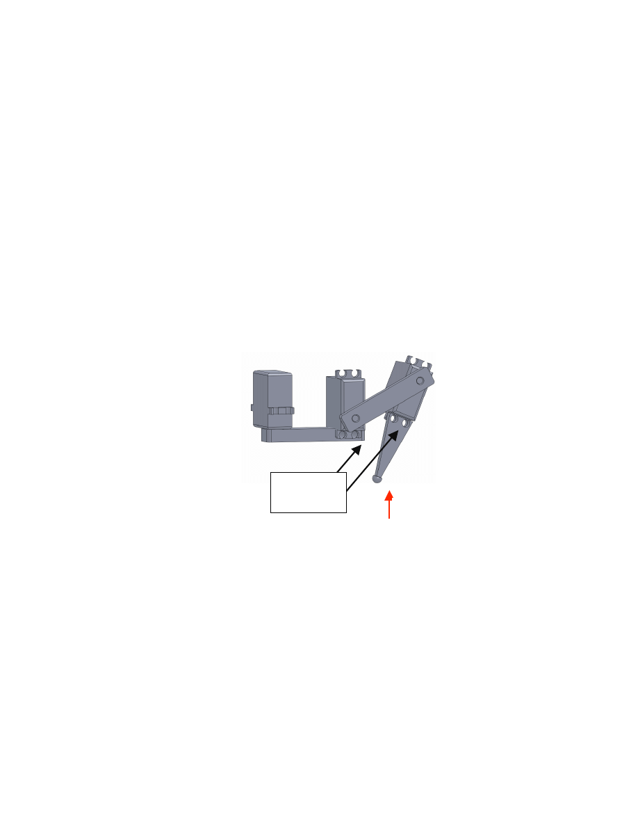
4.1 Securing
Servo
Motors


In
the
initial
design
for
the
leg,
the
servo
motors
were
mounted
to
the
leg
sections
using


only
two
connection
bolts.

It
was
determined
that
this
configuration,
shown
in
Figure
5,


would
concentrate
the
majority
of
the
weight
on
the
two
servo
contact
points.















Although
 the
 overall
 load
 would
 not
 be
 of
 a
 large
 magnitude
 the
 servo
 motors
 would


need
to
be
secured
tightly
to
eliminate
any
unnecessary
movement
of
the
servo
motor.
If


not
 secured
 tightly,
 the
 moment
 and
 shear
 force
 created
 at
 these
 two
 servo
 contact


points
will
loosen
the
fasteners
that
hold
the
servo
and
leg
sections
together.
The
design


was
therefore
changed
to
better
secure
the
servos
as
shown
in
Figure
6.
This
design
uses


all
four
connection
bolts
of
the
servo
mounting
flange.


Figure
5:
Selected
Design
with


body
weight
considerations


W
(body)


2
sets
of


fastening

contact
points


10











Figure
6:
Refined
Leg
Assembly,
using
all
four
bolt
holes.


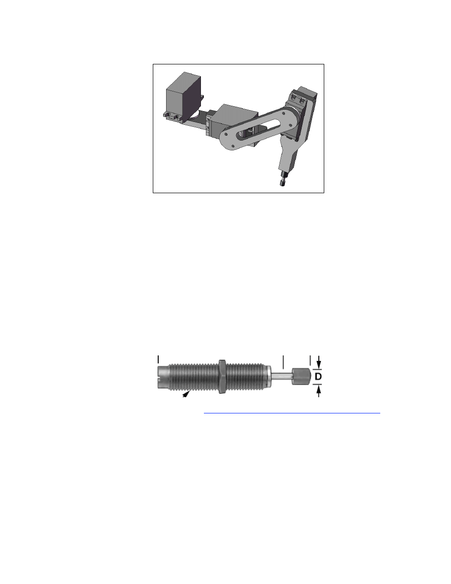
4.2 Suspension
and
Grip


The
hexapod
feet
were
modified
after
the
design
selection
to
provide
the
hexapod
with


some
 suspension
 and
 better
 grip
 during
 operation.
 The
 initial
 selected
 design
 shown
 in


Figure
5,
included
soft
rubber
padding
at
the
ends
of
the
legs
that
would
act
as
a
cushion


with
some
spring
characteristics.

Unfortunately
after
doing
some
research
into
possible


materials
it
was
found
that
for
the
scale
of
the
robot
most
rubber
materials
would
be
too


stiff
to
be
effective
shock
absorbers.
The
next
idea
was
to
use
a
set
of
shock
absorbers


shown
in
Figure
7
that
would
be
fastened
into
the
leg
ends
as
shown
in
Figure
6.








Figure
7:
Spring
rated
Shock
absorbers
(

http://www.mcmaster.com/catalog/114/gfx/large/3740kc1l.gif

)





The
issue
with
this
idea
was
that
the
Delrin
material
used
at
the
end
of
the
shocks
was


very
 slippery
 and
 would
 not
 provide
 adequate
 grip
 for
 walking.
 Since
 grip
 is
 very


important
for
motion
and
each
absorber
costs
$28.13,
which
is
high,
we
chose
to
use
a


contact
bumper,
shown
in
Figure
8.





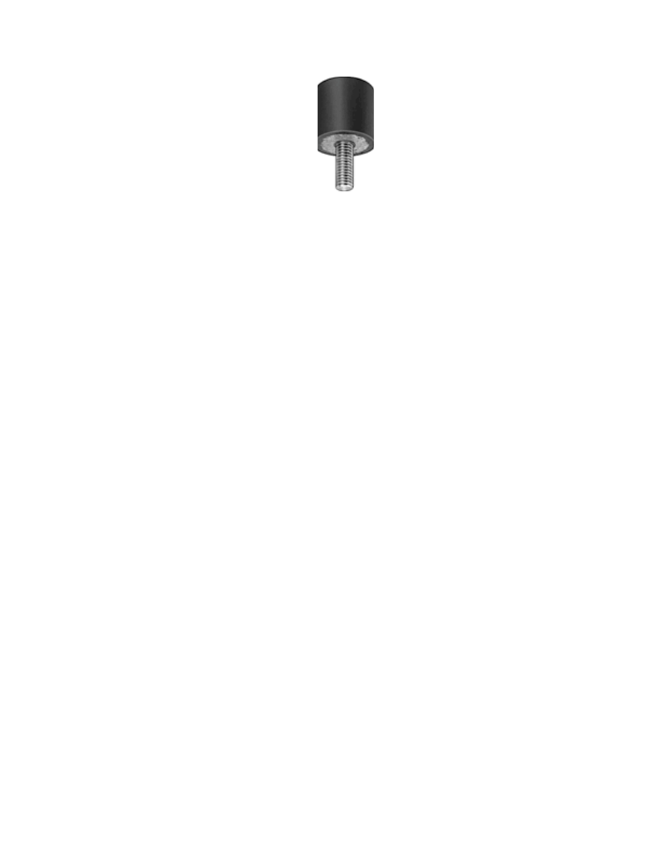
11








Figure
8:
Neoprene
Bumper
(http://www.mcmaster.com)





This
 bumper
 is
 made
 from
 neoprene,
 a
 material
 that
 provides
 better
 grip,
 and
 should


provide
some
spring
like
characteristics
for
a
smoother
walk
during
operation.


4.3 Rapid
Prototype


After
 receiving
 some
 suggestions
 from
 the
 technicians,
 the
 team
 decided
 to
 build
 a


prototype
 leg
 for
 control
 and
 possible
 destructive
 testing
 purposes.
 The
 hexapod
 leg


prototype
 was
 built
 using
 the
 rapid
 prototyping
 machine
 of
 the
 Dalhousie
 University


Mechanical
Engineering
Department.
The
process
took
a
total
of
three
hours
to
complete


and
cost
an
approximately
$14
to
build.
With
the
leg
prototype
built,
we
reassessed
the


design
and
found
that
the
end
leg
section,
with
the
threaded
hole,
would
be
better
if
it


was
 altered
 so
 that
 the
 threaded
 hole
 was
 centered
 on
 the
 mid‐plane
 of
 the
 piece.


Another
 design
 suggestion
 that
 came
 from
 the
 prototype
 leg
 was
 to
 drill
 a
 hole
 in
 the


second
section
of
the
leg
section
which
would
make
it
easier
to
assemble.
The
simplicity


of
the
rapid
prototype
method
of
producing
leg
sections
made
it
an
attractive
option
for


construction
of
the
final
product.
Testing
verified
the
rapid
prototype
plastic
would
be
of


adequate
strength
to
meet
design
requirements,
and
as
such
would
be
used
to
construct


the


finished


parts.


12








5 Final
Design


5.1 Overview


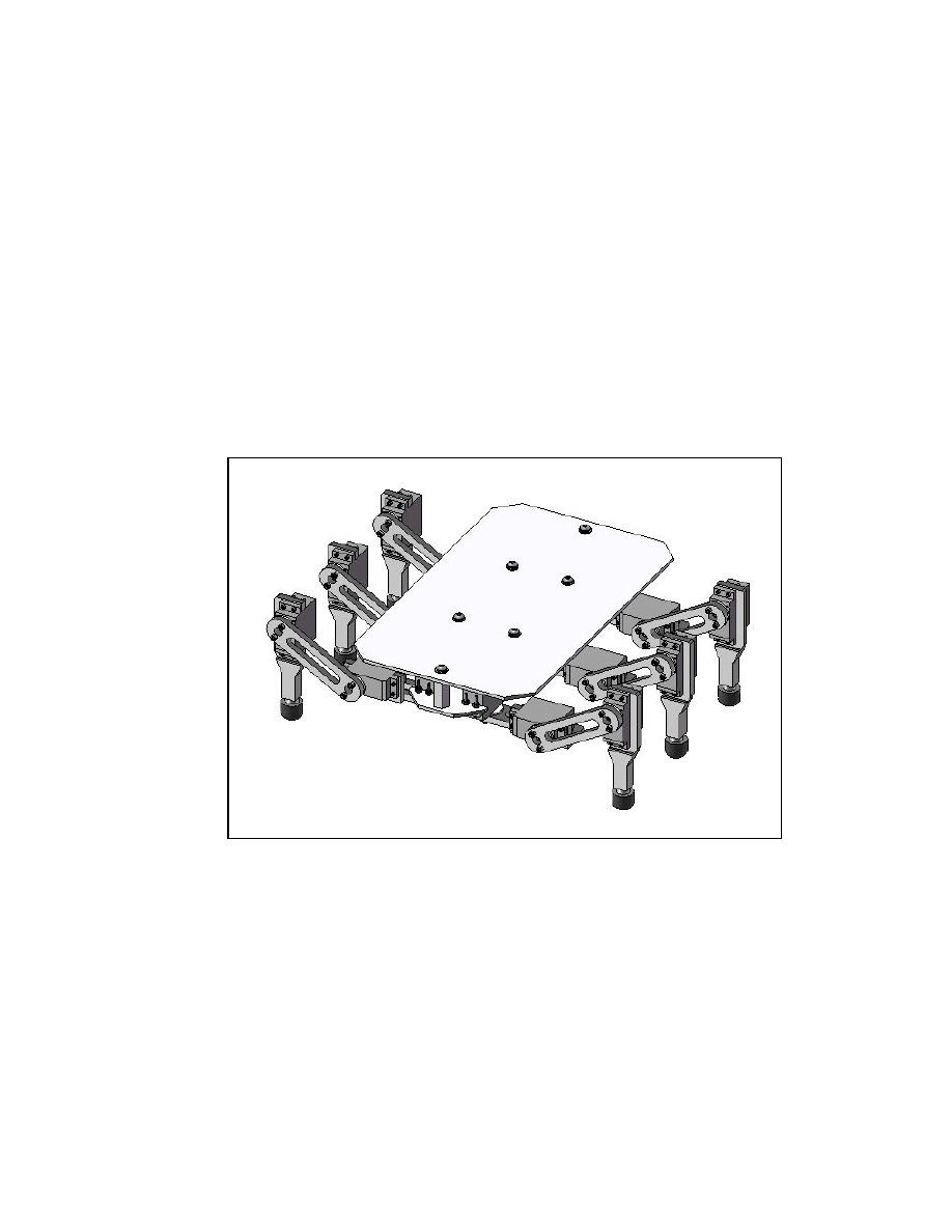
The
final
design
of
the
robot
was
arrived
at
after
the
improvements
from
the
design
refinement


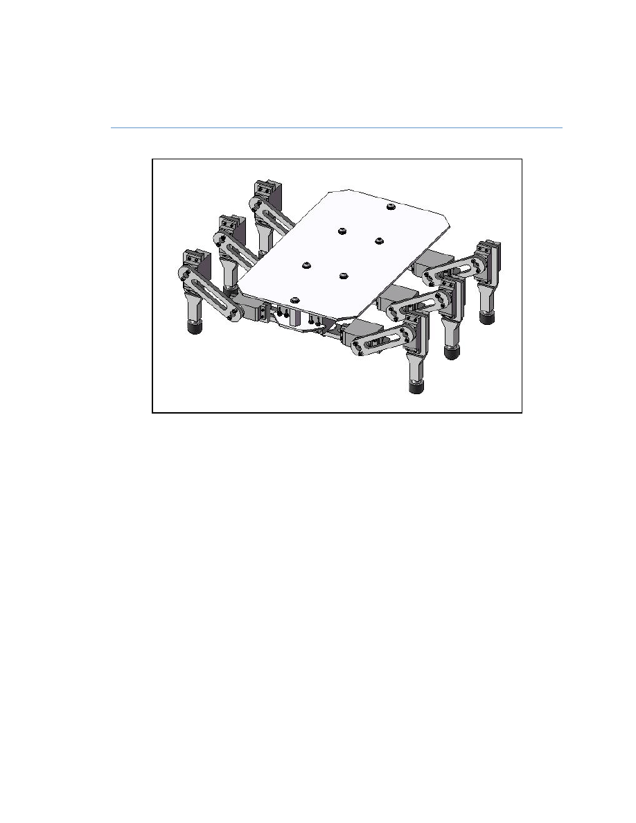
stage
were
incorporated
into
the
original
selected
design.
This
final
design
is
depicted
in
Figure


9.
There
are
six
modular
legs
that
connect
to
the
bottom
part
of
the
frame
and
there
is
plenty
of


space
available
on
the
top
plate
for
mounting
electronic
equipment.
All
fastening
details
have


been
worked
out
and
the
parts
are
ready
to
be
fabricated.
The
major
components
of
the
robot,


including
mechanical
and
programming
aspects,
will
now
be
presented
in
detail.





Figure
9
:
Final
Design
of
Hexapod
Robot


5.2 Frame


5.2.1 Description


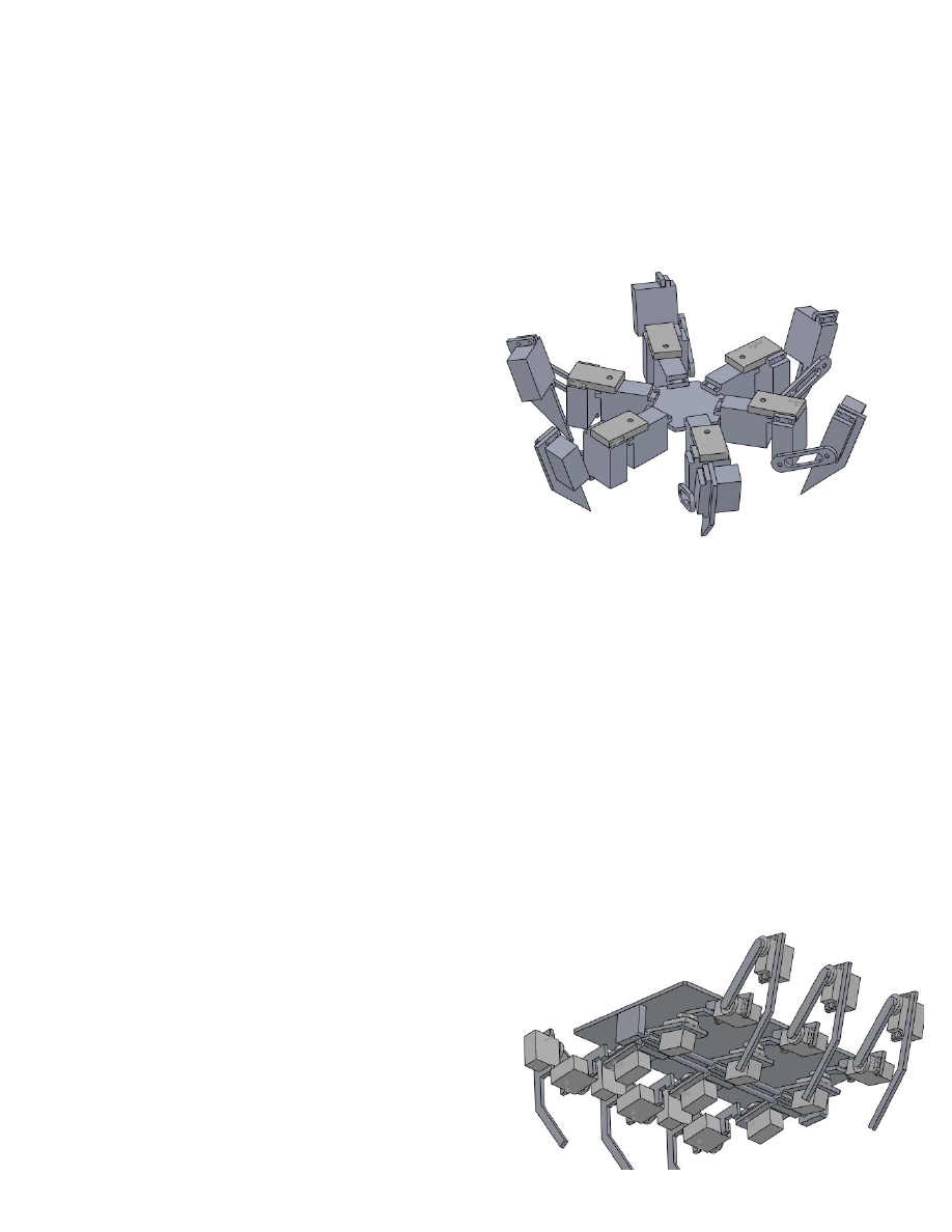
The
frame
of
the
robot
consists
of
two
.078”
aluminum
plates
that
are
bolted
together


using
six
commercially
available
standoffs,
as
illustrated
in
Figure
10.
The
smaller
plate
is


used
 for
 mounting
 the
 legs,
 while
 the
 larger
 plate
 is
 used
 for
 mounting
 electronic


equipment
such
as
the
microcontroller
boards.
As
well,
there
is
extra
space
on
the
large


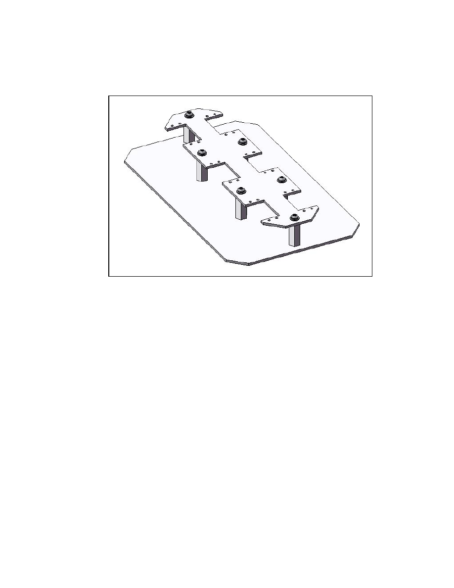
13





plate
so
additional
electronic
equipment
and
sensors
could
be
added
to
the
robot
in
the


future,
in
accordance
with
the
design
requirements.








Figure
10
:
Bottom
View
of
Frame
Assembly


5.2.2 Fabrication


The
 two
 aluminum
 plates
 will
 be
 machined
 and
 drilled
 by
 the
 department
 technician.


The
standoffs
are
a
purchased
part
and
come
threaded
at
both
ends.
Assembly
is
simple


and
will
be
done
by
the
team.


5.2.3 To
Be
Determined


The
 large
 plate
 is
 used
 for
 mounting
 the
 electronic
 equipment.
 This
 includes
 the
 two


microcontrollers
as
well
as
any
additional
sensors
that
might
be
added
later
on
in
the


project.
Cutouts
will
need
to
be
made
in
the
large
plate
to
allow
wires
to
pass
through.


The
 layout
 of
 the
 electronic
 equipment
 and
 associated
 cutouts
 has
 not
 been
 finalized


yet.
However,
this
is
not
a
pressing
issue
and
will
wait
for
final
assembly.


5.3 Legs


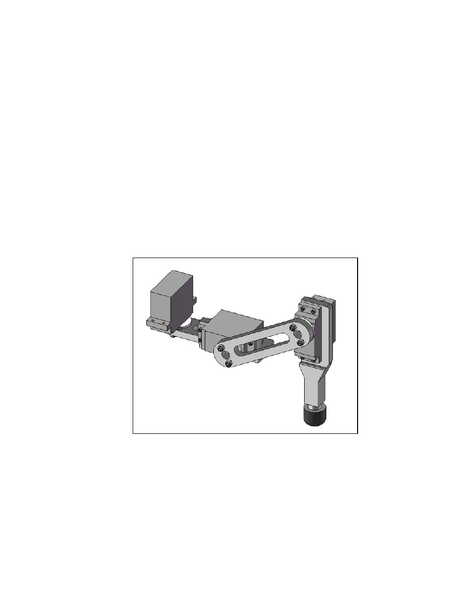
5.3.1 Description


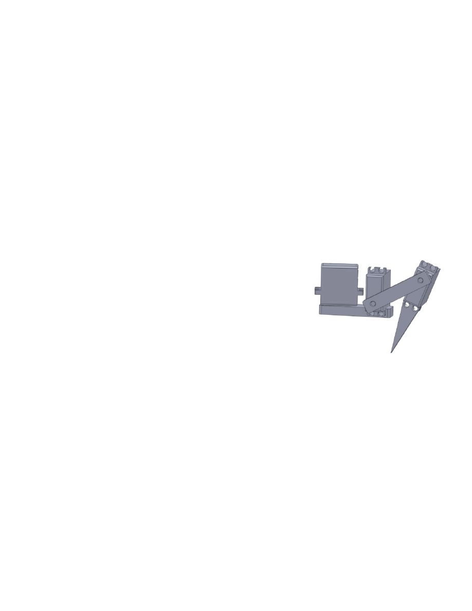
Each
 of
 the
 six
 legs
 will
 contain
 three
 servomotors
 that
 are
 connected
 by
 three
 leg


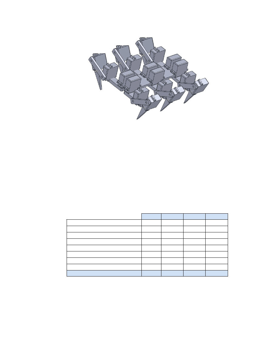
sections
 as
 shown
 in
 Figure
 11.
 For
 a
 better
 view
 of
 the
 individual
 leg
 sections,
 see


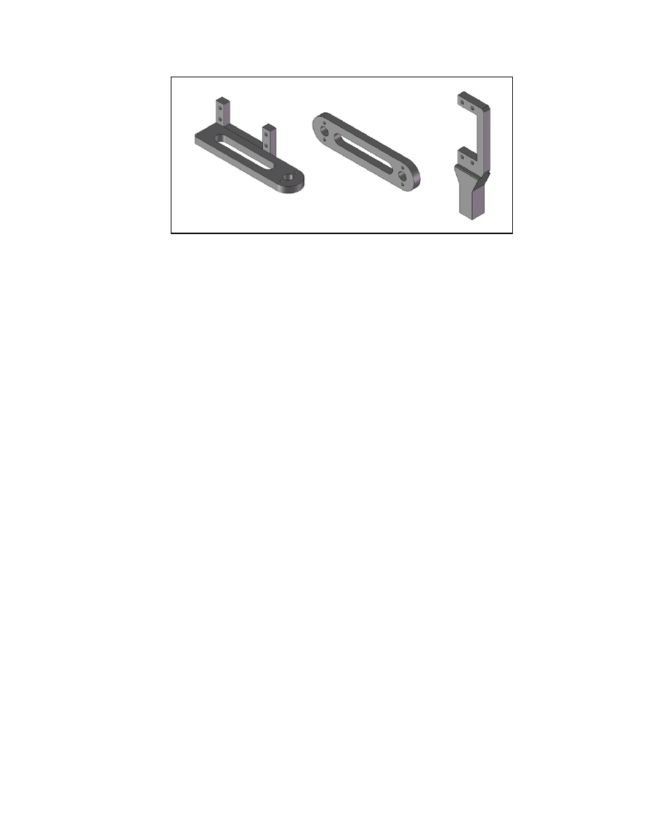
Figure
12.
The
leg
sections
are
named
as
the
first,
second
and
third
leg
sections,
with
the


14





first
 leg
 section
 being
 the
 one
 joined
 to
 the
 frame.
 
 They
 are
 simple
 pieces
 and
 are


shaped
in
a
manner
that
allows
simple
connections
with
the
servomotors.
Additionally,


there
 are
 small
 neoprene
 feet
 (commercially
 available)
 that
 thread
 into
 the
 third
 leg


section.
These
will
provide
adequate
traction
as
well
as
shock
absorption
to
reduce
the


stress
within
the
joints.


Each
 leg
 section
 will
 be
 manufactured
 using
 the
 Mechanical
 Department’s
 rapid


prototype
machine.
Afore
mentioned
testing
has
verified
that
the
parts
will
be
robust


enough
to
meet
design
requirements
and,
due
to
the
prototyping
process,
be
available


at
 a
 much
 earlier
 date.
 The
 inner
 and
 outer
 leg
 sections
 will
 come
 in
 a
 left
 and
 right


handed
 variety
 while
 the
 middle
 leg
 section
 will
 be
 the
 same
 on
 both
 sides.
 The
 leg


sections
will
be
bolted
to
the
servomotors
using
small
#2
bolts
at
the
servo
mounting


flanges
and
at
the
servos
mounting
disk
(attached
to
output
shaft).








Figure
11
:
Leg
Assembly


15








Figure
12
:
Three
Leg
Sections,
named
as
the
“First,
Second
and
Third
leg
sections”
(left
to
right)


5.3.2 Fabrication


Manufacturing
of
the
leg
sections
will
be
performed
from
Solid
Works
drawings
produced
during


the
 design
 stages.
 These
 drawings
 are
 forwarded
 to
 Craig
 Arthur
 to
 be
 set
 to
 run
 on
 the


prototyping
 machine.
 The
 final
 parts
 will
 come
 out
 needing
 small
 modifications
 to
 remove


support
material.
Reaming
holes
to
finished
diameter
will
be
completed
by
the
team,
as
well
as


drilling
of
mating
holes
in
the
servo
mounting
flanges.
All
final
assembly
will
be
completed
by


team
members.





Technician
time
is
required
to
machine
aluminum
components
and
is
detailed
in
table
3.


5.4 
 Control
Hardware


5.4.1 Description


To
control
the
hexapod’s
movements,
two
boards
would
be
used:

a
servo
control
board


to
send
timed
pulses
capable
of
setting
servo
positions,
and
a
microcontroller
to
send


and
receive
signals
onboard
the
hexapod.



To
control
servos,
a
Devantech
SD‐21
Servo
Control
Board
was
selected.
In
addition
to


its
low
cost,
the
SD‐21
has
pin
connections
for
up
to
21
servos
for
which
it
can
control


the
position
and
speed
through
integer
inputs.
The
board
will
satisfy
the
‘expandability’


component
of
the
design
by
allowing
an
additional
3
servos
for
an
added
task
specific


appendage.
 The
 SD‐21
 is
 capable
 of
 receiving
 a
 basic
 stamp
 controller
 via
 one
 of
 two


standard
 sockets,
 and
 can
 communicate
 with
 an
 external
 controller
 through
 any
 of


three
I

2

C
connections.
The
latter
option
will
be
utilized
in
this
design.



16





For
 the
 external
 microcontroller
 option
 used
 in
 this
 design,
 an
 Arduino
 Decimilla
 was


selected
as
its
internal
Wire
library
and
I

2

C
pins
would
allow
simple
interfacing
with
the


SD‐21.
 In
 addition,
 the
 Decimilla
 uses
 an
 onboard
 serial
 converter
 so
 that
 a
 common


USB
A
to
B
cable
can
be
used
to
interface
with
a
computer
for
serial
communication.


The
Decimilla
has
the
added
advantage
of
available
analog
and
digital
in/outputs,
also


satisfying
the
expandability
requirement.


5.4.2 Fabrication


To
put
a
polished
look
on
the
controlling
hardware,
interconnects
that
utilize
headers
to


connect
 to
 both
 the
 male
 and
 female
 I

2

C
 ports
 will
 be
 fabricated
 by
 the
 group.
 The


interconnect
cables
will
be
labeled,
or
of
a
design
such
that
the
hexapod’s
electronics


cannot
be
incorrectly
assembled.






The
boards
will
be
mounted
to
the
robot’s
top
plate
using
hex
standoffs
and
all
servo


cables
will
be
bundled
and
routed
through
the
hexapod’s
body.


5.4.3 To
Be
Determined


Final
 positioning
 has
 not
 yet
 been
 determined.
 Cable
 routing
 will
 determine
 the
 final


position
of
the
boards,
and
this
cannot
be
finalized
without
a
final
model.
Mounting
is


uncomplicated
and
will
require
very
little
fabrication
making
it
an
acceptable
TBD
item.






5.5 Control
Software


Software
 development
 will
 take
 place
 within
 Matlab
 using
 .m
 files.
 The
 programming


can
 be
 broken
 into
 3
 major
 components:
 motion
 planning,
 conversion,
 and


communication.


5.5.1 Motion
Planning


There
are
two
ways
to
control
the
hexapod
robot.
One
involves
having
a
set
routine
in


which
 every
 angle
 and
 timing
 pause
 are
 pre‐defined.
 The
 second
 and
 more
 complex


option
 involves
 telling
 what
 you
 want
 to
 robot
 to
 accomplish
 and
 the
 software


determine
the
leg
path
along
with
the
necessary
servo
angles
to
perform
the
maneuver.


The
hexapod
robot
will
use
the
second
option
which
will
give
the
robot
more
flexibility


and
a
smoother
movement.


17





Currently
ongoing
work
involves
writing
an
inverse
kinematics
(IK)
program
in
which
the


user
of
a
path
creation
program
defines
two
points
of
the
leg
movement,
the
start
and


end
point.
From
the
know
point,
IK
solves
for
the
servo
angle
which
will
move
the
end


effector
to
its
new
position.


In
order
to
determine
the
servo
angle,
the
3DOF
problem
was
redefined
as
a
1DOF
and
a


separate
 2DOF
 problem.
 This
 modification
 was
 possible
 since
 only
 the
 first
 servo
 was


capable
of
moving
the
leg
in
the
back
and
forth
direction.
The
servo
also
produces
no


movement
in
the
z
direction.
After
the
leg
is
pointed
towards
the
end
effector
location,


the
 other
 two
 servos
 are
 responsible
 for
 extending
 the
 leg
 the
 correct
 distance
 and


providing
the
body
lift.
All
servo
angles
are
determined
by
trigonometry
but
the
last
two


are
dependent
on
each
other
therefore
simultaneous
equations
must
be
solved.



Once
the
IK
program
was
written,
leg
path
programming
was
the
next
step.
A
program


which
takes
two
points,
in
X,Y
coordinates,
along
with
ROV
body
height
and
step
height


was
 created.
 It
 creates
 a
 parabola
 between
 both
 points
 and
 divides
 it
 into
 discrete


points
 which
 the
 IK
 program
 calculates
 the
 angles
 required
 for
 each
 point
 and
 stores


them
into
a
larger
matrix.


To
date,
the
software
is
capable
of
defining
the
proper
servo
angle
to
make
the
robot


leg
complete
one
entire
step
between
any
two
arbitrary
points.





5.5.2 Conversion


The
 resulting
 output
 of
 the
 Motion
 Planning
 software
 will
 be
 in
 degrees
 and
 time


intervals.
 This
 data
 will
 need
 to
 be
 converted
 to
 be
 understood
 by
 the
 SD‐21
 servo


control
 board.
 The
 SD‐21’s
 internal
 register
 stores
 four
 numbers
 pertaining
 to
 each


servo:
a
servo
call,
speed,
and
two
positioning
numbers.
The
servo
call
is
a
number
given


to
each
servo’s
registry
spaces.
When
the
servo
call
is
sent
to
the
SD‐21,
the
following
3


numbers
will
be
assigned
to
the
speed
and
position
spaces.
The
speed
number
is
set
to
0


for
 full
 speed,
 or
 numbers
 1
 through
 9
 for
 slower
 movement.
 Finally,
 the
 position


numbers
 are
 the
 low
 and
 high
 bytes
 of
 the
 desired
 pulse
 width
 integer.
 Testing
 has


revealed
that
for
the
selected
servos,
the
pulse
widths
used
from
lock
to
lock
are
in
the


18





700‐2500
 (micro‐second)
 range.
 The
 pulse
 width
 steps
 correspond
 to
 degrees


proportionally
using
the
following
formula:


∆ =
10∗∆ 



(3)


Where:









∆


=
Desired
change
in
degrees








∆


=
Change
in
pulse‐width





The
 output
 of
 the
 conversion
 from
 degrees
 will
 be
 an
 integer
 within
 the
 pulse
 width


range.
 The
 integer
 needs
 to
 be
 split
 into
 integer
 representations
 of
 the
 high
 and
 low


bytes
of
this
number.
These
parts
may
be
found
by
converting
to
hexadecimal:
the
high


byte
will
be
the
first
integer
value,
while
the
low
byte
will
be
the
remainder
once
the


high
 byte
 has
 been
 multiplied
 by
 256
 and
 subtracted
 from
 the
 original
 value.
 A


converting
algorithm
has
been
written
and
is
incorporated
in
the
preliminary
software


appendix
package.







5.5.3 Communication


Once
the
appropriate
conversion
has
taken
place,
the
data
is
stored
in
matrices
of
leg


positions
 within
 Matlab.
 The
 matrices
 match
 the
 register
 on
 the
 SD‐21
 board
 and
 are


sent
 through
 the
 serial
 port
 to
 the
 Decimilla
 for
 storage
 to
 be
 sent
 to
 the
 SD‐21
 in
 a


timed
 sequence
 corresponding
 to
 the
 desired
 gait.
 Matlab’s
 serial
 communication


commands
simplify
this
procedure.
An
additional
serial
monitor
is
added
to
open
TX
and


RX
pins
on
the
Arduino
board
for
debugging
purposes.






Once
 the
 gait
 has
 been
 calculated
 and
 stored
 on
 the
 Decimilla,
 the
 register
 must
 be


updated
with
positions
corresponding
to
leg
points.
The
Arduino
board
is
able
to
open
a


connection
 with
 the
 SD‐21
 (using
 the
 aforementioned
 I

2

C
 ports),
 update
 the
 register,


and
 close
 the
 connection.
 This
 sets
 the
 servos
 in
 motion,
 roughly
 following
 the
 path


calculated
in
the
motion
planning
stage.





19








6 Testing


6.1 Finite
Element
Analysis
(FEA)


The
 strength
 of
 the
 leg
 links
 was
 a
 concern.
 A
 preliminary
 finite
 element
 analysis
 was


performed
to
ensure
theses
links
would
not
fail
in
tension
or
compression.
The
leg
section


subjected
to
the
highest
loading
is
the
first
section
since
it
must
support
the
load
of
the


robot
and
the
torque
of
the
servo
along
its
axis
of
minimum
moment
of
inertia.
Therefore


only
this
link
will
be
tested.


6.1.1 Model
Description


Since
 only
 a
 rough
 stress
 profile
 was
 desired,
 it
 was
 appropriate
 to
 quickly
 mesh
 the


model
 using
 3D
 tetrahedral
 elements.
 Another
 advantage
 to
 the
 tetrahedrons
 is
 the


ability
 to
 auto‐mesh
 the
 solid
 part.
 An
 initial
 element
 size
 of
 1.5mm
 was
 used,
 then


varied
up
to
3mm
and
down
to
0.75mm
to
ensure
a
consistent
result.


The
 Program
 used
 in
 this
 analysis
 is
 Unigraphics
 NX
 5.0
 which
 uses
 the
 Nastran
 NX


solver.
 The
 material
 model
 used
 was
 the
 pre‐defined
 NX
 5.0
 model
 for
 PVC,
 which


include
a
Young’s
modulus
of
300
MPa
and
a
Poisson’s
ratio
of
0.4.



The
 loading
 for
 the
 leg
 linkage
 was
 composed
 of
 two
 parts,
 the
 vertical
 force
 which


keeps
the
robot
suspended,
and
the
torque
produced
by
the
servo.
The
Vertical
force


used
was
9.4N
which
simulated
the
9.8Kg*N
of
torque
applying
a
force
6
cm
from
the


rotation
 axis.
 The
 torque
 applied
 was
 0.981
 N*mm
 which
 is
 the
 rated
 capacity
 of
 the


servo
itself.


To
simulate
being
attached
to
a
servo
at
the
body,
the
two
smaller
mounting
holes
seen


at
the
bottom
right
of
Figure
13
where
fixed
in
all
6
DOF.


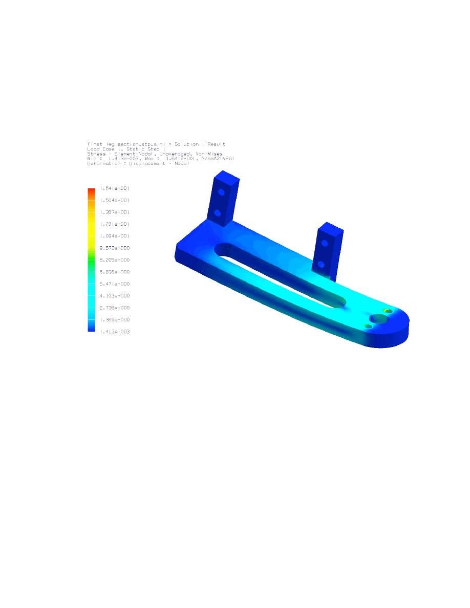
6.1.2 Results


After
running
the
simulation,
the
Von‐Mises
stress
(

)


was
plotted.
This
stress
is
the


equivalent
stress
and
is
used
to
compare
for
failure
against
the
yield
stress
(

)


of
the


material.
 In
 this
 case,
 failure
 is
 defined
 as


>

.
 As
 seen
 in
 Figure
 13
 below,
 the


Von‐Mises
stress
found
through‐out
most
of
the
link
is
approximately
6MPa.
This
value


is
much
lower
that
the



of
PVC
which
is
40
MPa.



20





It
can
also
be
seen
that
the
stress
peaks
are
around
the
mounting
holes.
The


is
still


only
16.4
MPa.
The
team
believes
this
value
is
much
higher
than
would
be
seen
on
the


actual
part
since
the
model
is
stiffly
constrained
whereas
the
actual
link
is
clamped
and


slight
motion
is
allowed.
Even
with
a
moderate
to
low
accuracy,
the
results
conclude
the


part
will
not
fail.





Figure
13:
Von‐Mises
Stress
of
the
First
Bar
Linkage





6.2 Hexapod
Motion
Simulations


Simulation
models
are
useful
in
refining
the
controlling
schemes
before
applying
them
to


the
 real
 system.
 Simulations
 can
 also
 be
 used
 to
 check
 for
 design
 issues
 such
 as


interference
 within
 a
 model.
 The
 motions
 of
 the
 hexapod
 can
 be
 simulated
 in


programming
 software
 called
 Matlab.
 This
 is
 accomplished
 by
 using
 a
 combination
 of


Matlab’s
specialized
Simulink
and
Virtual
reality
toolbox
add‐ons.




6.2.1 Simulink


Simulink
 is
 a
 system
 modeling
 interface
 tool
 that
 can
 read
 in
 inputs
 from
 Matlab,


perform
 analysis
 on
 the
 inputs
 if
 necessary,
 and
 output
 the
 results
 for
 graphing
 and


21





other
 uses
 such
 as
 simulations.
 Simulink
 uses
 a
 ‘block’
 style
 structure
 in
 manipulating


data
and
performing
calculations.





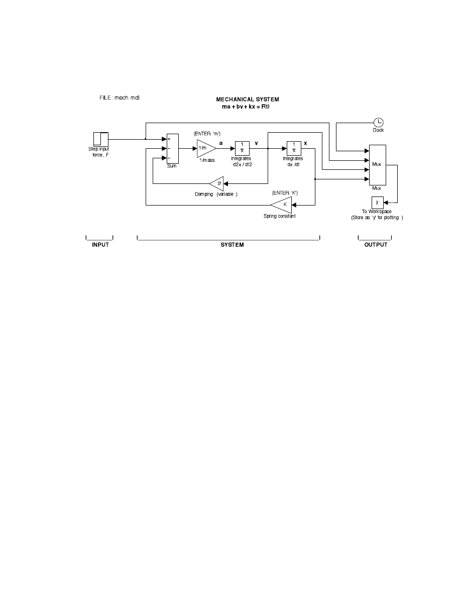
Figure
14:
Block
Diagram
representation
of
a
differential
mechanical
system


[Bauer,
Robert;
“MECH
3900:
Assignment
1”;
‘Department
of
Mechanical
Engineering
Dalhousie
University,
Jan


15,2008]


Figure
14
shows
a
common
block
diagram
representation
of
a
system
model
defined
in


Simulink.




In
this
block
diagram
the
input
data
is
provided
by
the
Matlab
driving
routine.


Values
for
all
the
blocks
can
be
provided
by
the
Matlab
code
or
can
be
initialized
in
the


Simulink
blocks.
The
output
data
is
combined
into
an
array
using
the
MUX
block
and
is


then
 sent
 to
 the
 workspace.
 The
 workspace
 could
 be
 anything
 from
 a
 graph
 to
 the


original
driving
routine
for
further
manipulation.


6.2.2 Virtual
Reality
Toolbox



Virtual
Reality
toolbox
is
a
program
that
uses
the
position
and
angle
data
supplied
by


Simulink
to
visually
show
the
simulation
of
a
model
in
the
Virtual
World.

A
solid
works


model
of
the
hexapod
is
inserted
into
the
Virtual
World
and
can
be
simulated
using
data


generated
by
Matlab.
In
the
case
of
the
hexapod
robot
simulation
the
input
code
into


Simulink
 will
 be
 a
 ‘driving
 routine’
 gait
 motion
 code
 (Appendix
 D)
 which
 has
 been


written
in
Matlab.
The
Virtual
Reality
Toolbox
sink
block
connects
the
output
Simulink


data
to
the
Virtual
object
(which
is
the
hexapod
legs
for
our
case)
located
in
the
virtual


reality
world.


22





6.3 Working
Leg


A
 working
 prototype
 leg
 has
 been
 manufactured
 and
 tested
 as
 of
 November
 26,
 2008.


The
 single
 leg
 was
 built
 as
 a
 proof
 of
 concept.
 A
 finished
 leg
 is
 required
 to
 proceed
 on


hardware
testing
and
to
set
the
initial
positions
of
each
servo,
thus
creating
a
need
for
the


model.



6.3.1 Mechanical


With
an
existing
solid
works
model,
a
rapid
prototype
version
of
the
leg
joints
was
found


to
 be
 the
 timeliest
 method
 of
 manufacturing
 the
 needed
 leg
 sections.
 The
 plastic


material
 used
 by
 Dalhousie’s
 rapid
 prototype
 machine
 was
 considered
 strong
 enough


for
 preliminary
 testing,
 as
 its
 material
 properties
 closely
 matched
 the
 final
 design


material.
 The
 three
 leg
 sections
 were
 prototyped
 and
 assembled
 using
 three
 Hi‐Tec


brand
servos.



Some
 minor
 alterations
 from
 the
 original
 design
 came
 from
 assembly
 of
 the
 rapid


prototyped
leg
members.
For
reduction
of
weight,
the
first
leg
section
would
have
a
slot


cut
through
the
center,
as
in
the
second
leg
section.
To
aid
in
assembly,
all
servo
disk


mounting
positions
would
have
a
through
hole
drilled
to
access
the
servo
shaft
spline


bolt
that
holds
the
mounting
disk
in
place,
making
assembly
and
disassembly
an
easier


process.


6.3.2 Hardware


A
power
supply
was
procured
to
power
the
servos
through
a
temporary
power
cable.


The
5V
section
of
the
supply
was
used
to
limit
servo
performance
for
initial
testing.
In


future
 testing
 a
 9.6
 volt
 supply
 will
 be
 used.
 The
 SD‐21
 board
 logic
 section
 was


temporarily
powered
through
a
jumper
from
the
servo
supply
side.
However,
in
future


iterations
the
SD‐21
will
be
powered
by
the
Arduino
which
is
supplied
by
the
USB
port.



The
Arduino
and
SD‐21’s
I

2

C
ports
were
connected.


6.3.3 Software


All
 values
 of
 speed,
 low
 and
 high
 bytes
 were
 calculated
 using
 initial
 versions
 of
 the


Matlab
software
included
in
the
appendix.
These
positions
were
then
manually
entered


into
arrays
in
the
Arduino
board,
as
serial
communication
is
not
yet
fully
debugged.
As


23





will
be
used
in
the
final
version,
three
positions
were
entered
to
form
a
leg
path,
which


is
followed
on
each
run
of
the
Arduino’s
program,
as
seen
in
the
appendix.



The
 leg’s
 performance
 is
 as
 expected
 and
 further
 testing
 will
 provide
 preliminary


performance
numbers
for
speed
and
weight
carrying
capacity.



24








7 Project
Status


7.1 Progress


The
team
has
currently
finalized
its
design
selection.
All
drawings
and
specifications
have


been
completed
along
with
some
proof
on
concept
work.
This
work
includes
the
virtual


modeling
of
the
leg
kinematics
and
the
building
of
a
prototype
leg.


The
software
is
still
currently
being
worked
on
and
is
showing
promise.
The
IK
program


has
been
successful
in
defining
the
correct
angle
changes
to
reposition
the
final
two
links


of
the
leg.
The
Matlab
transmission
program
has
also
been
able
to
give
basic
control
to


the
mock‐up
leg
in
order
to
perform
a
single
crude
step.


The
 group
 also
 believes
 they
 have
 completed
 the
 appropriate
 amount
 of
 modeling
 and


testing
 to
 begin
 production
 of
 the
 six
 legs
 and
 body
 in
 order
 to
 have
 a
 fully
 assembled


model
early
in
the
second
term.
The
improvement
of
the
software
will
be
continual
until


the
end
of
term
to
achieve
the
best
results
possible
within
the
allotted
timeframe.


7.2 Technician
Time


All
fabrication
work
will
be
completed
by
the
department.
This
is
limited
to
the
cutting


and
machining
of
parts.
This
will
ensure
quality
fabrication
of
components.
An
estimate
of


the
machining
time
required
from
the
department
for
this
project
is
provided
in
Table
3.





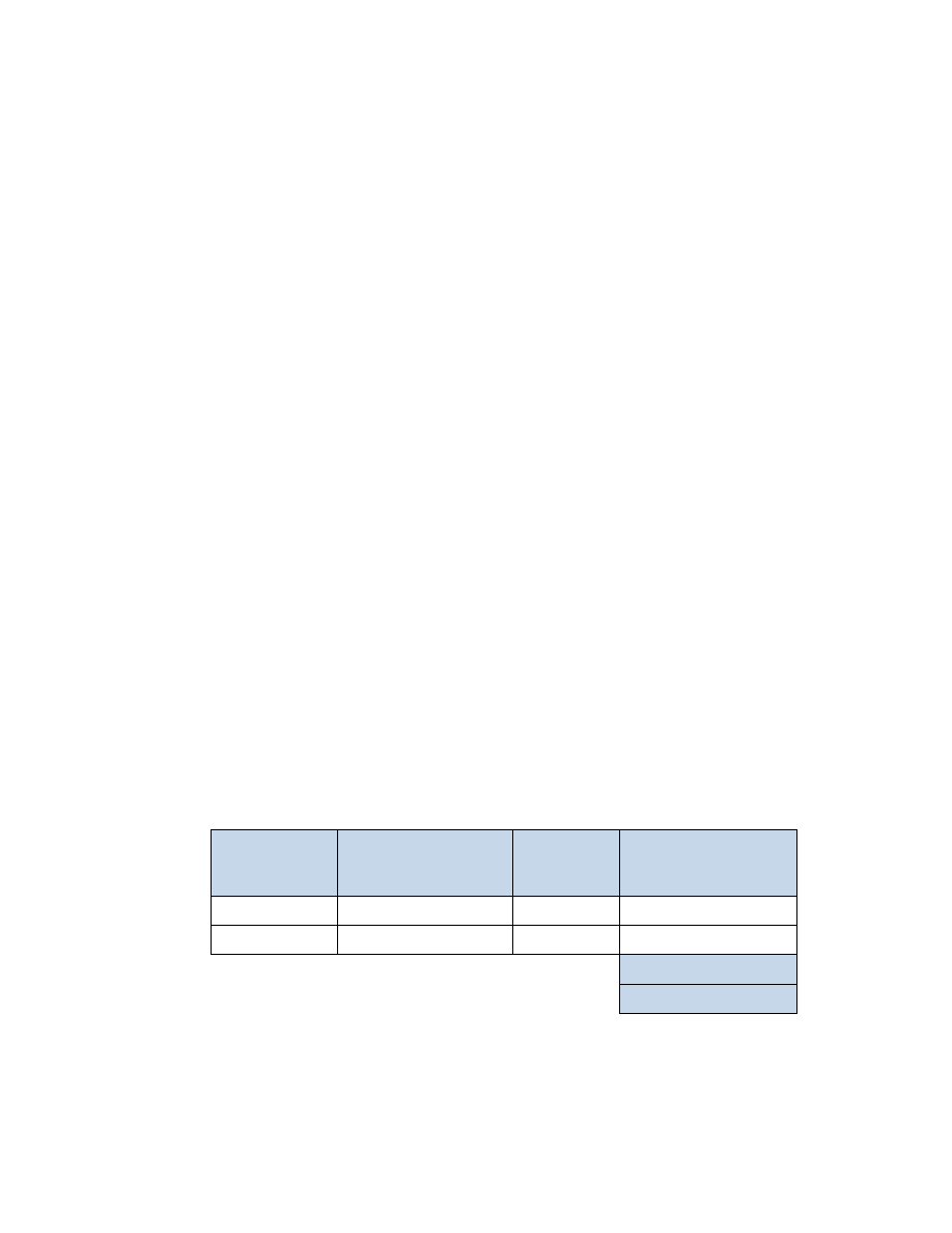
Table
3:
Estimated
Machining
Time
Required
from
Department


Part
Number


Part
Description


Quantity


Total
MachiningTime


(hrs)


HX‐0012


Top
Plate


1


1.5


HX‐0013


Bottom
Plate


1


4











Total











5.5







25





All
assembly
work
will
be
completed
by
the
team.
Assembly
requires
the
use
of
simple
hand


tools
and
bonding
agents.
Advice
may
be
sought
from
the
technicians
during
the
assembly


process.


8 Budget


With
the
selected
design
being
finalized,
Team
#2
has
assembled
the
budget
found
in
Table
4.

To
date
we
have
secured
$1800
of
our
project
cost.


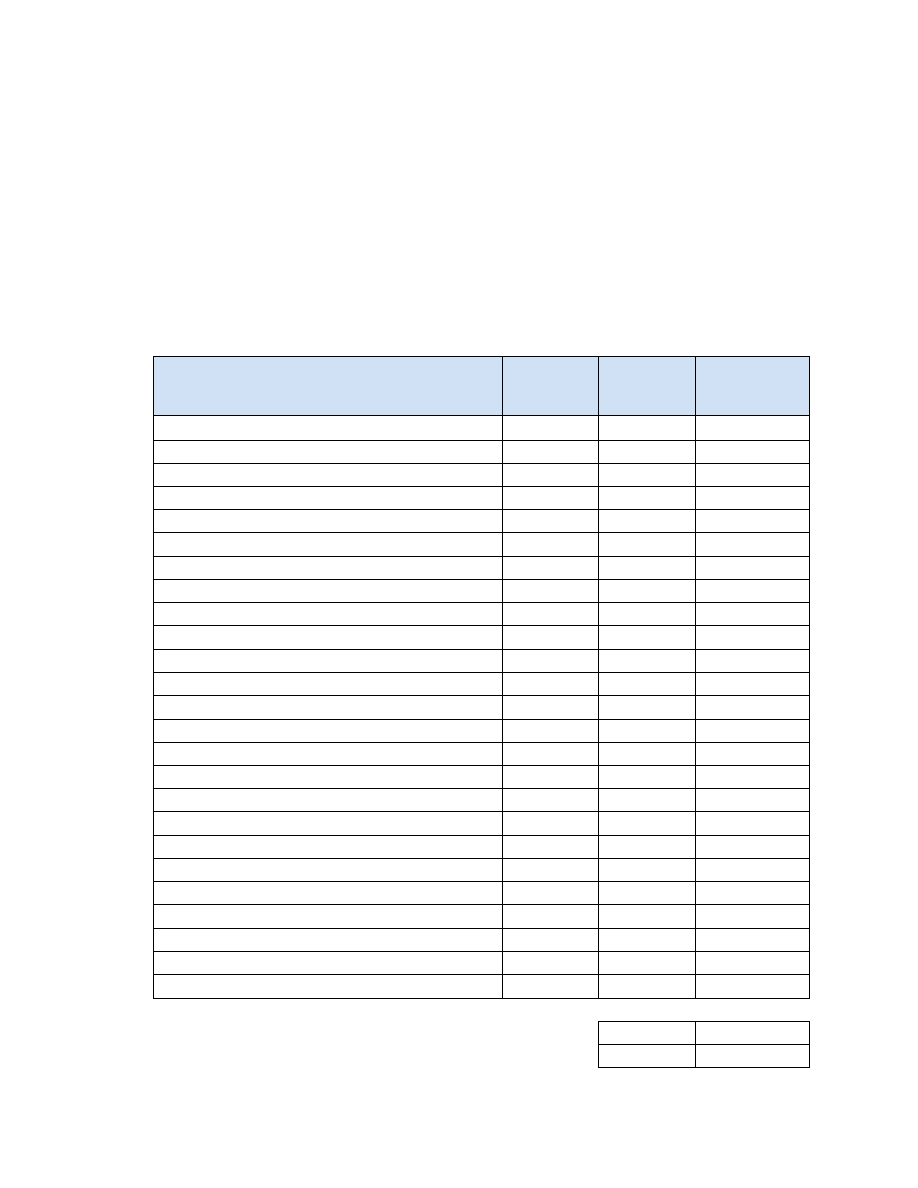
Table
4:
Proposed
Budget


Materials


Unit


cost


Amount


Cost


Electronics











HS‐645MG
Servos


$39.02


21


$819.42


HS‐765HB


$43.78


1


$43.78


HS‐805BB


$43.36


1


$43.36


25'
22g
black
wire


$2.62


1


$2.62


25'
22g
red
wire


$2.62


1


$2.62


Netmedia
6"
jumper
Wire
kit


$8.49


1


$8.49


Eneloc
30
pc.
Reinforced
Jumper
wire
kit


$18.91


1


$18.91


Pulse
Width
Modulator


$63.15


2


$126.30


USB
Cable


$2.99


1


$2.99


Microcontroller


$40.64


1


$40.64


Resistors
(500
ohm
+
2000
ohm)


$1.00


2


$2.00


Potentiometer
(500ohm)


$7.85


1


$7.85


Rocker
Switch


$1.39


1


$1.39


Protoboard


$15.00


1


$15.00


Raw
Materials













3/8"
Hex
Standoff
1/8"PL


$1.00


12


$12.00


1/4"
ABS


$13.29


3


$39.87


1/2"
ABS


$27.39


2


$54.78


1/8"Alluminum
Plate
6061


$26.06


3


$78.18


Plastic
Bonder


$24.99


1


$24.99


1‐1/4"
AL
Hex
Standoff

10‐32
screw


$3.03


6


$18.18


Leg
Bumper


$6.23


7


$42.00


Fastners


$20.00


1


$20.00


Rapid
prototyping


$7.00


3


$21.00




















Subtotal


$1,383.22








Tax
(15%)


$207.48


26











Shipping


$100.00








Total


$1,690.70


27








9 Conclusion
and
Recommendations





Hexapod
robot
is
a
relatively
inexpensive
and
capable
machine.
The
servo
arrangement
allows


the
 robot
 to
 maneuver
 with
 relative
 ease
 in
 both
 planar
 directions.
 The
 three
 degrees
 of


freedom
 per
 leg
 also
 allows
 the
 ROV
 to
 adjust
 its
 height
 without
 affecting
 the
 other


performance
 characteristics.
 The
 large
 plate
 forming
 the
 top
 of
 the
 body
 allows
 for
 the


mounting
of
circuit
boards
and
additional
sensors
improving
the
versatility
of
the
robot.





Several
design
choices
were
evaluated
before
the
final
design
was
chosen.
The
main
differences


between
the
alternative
designs
were
the
positioning
and
design
of
the
six
legs.
Increasing
the


complexity
 of
 the
 robot
 was
 investigated
 but
 not
 done
 due
 to
 the
 difficulty
 on
 building
 the


model
and
the
extra
complexity
of
the
motion
programming.
One
alternative
design
had
the
six


legs
spread
evenly
along
a
hexagonal
body
shape.
This
improved
the
rotation
capabilities
of
the


hexapod,
but
since
the
ROV
would
have
no
front
or
back
end,
each
leg
has
to
be
programmed


individually
 even
 to
 perform
 the
 simple
 tripod
 gait.
 The
 team
 selected
 a
 ROV
 consisting
 of
 a


rectangular
body
and
the
six
legs
being
spread
equally
along
both
sides.
This
maximized
both


the
maneuverability
and
programming
simplicity.





Several
tests
were
performed
to
ensure
the
legs
had
appropriate
range
of
motion
and
strength


to
 support
 the
 hexapod.
 These
 test
 included
 a
 FEA
 analysis,
 a
 virtual
 simulation
 in
 MATLAB


SImulink
and
then
the
construction
of
a
prototype
leg.

With
the
validation
of
our
design,
the


group
is
ready
to
begin
fabrication
of
the
entire
hexapod
ROV.


28





Appendix
A:
2
DOF
Inverse
Kinematic
MATLAB
program




User
must
manually
input
the
initial
and
final
leg
position
along
with
the
body
height,
step

height,
and
number
of
points
along
the
parabola.






clc

clear

P1=[0.15 0.02; 0.16 0]

body_height=0.08;

step_heigth=0.03;

point_num=4;

steplength=sqrt((P1(2,1)-P1(1,1))^2+(P1(2,2)-P1(1,2))^2)

% Defining the polynomial

x=[0 steplength/2 steplength];

y=[0 step_heigth 0];

p=polyfit(x,y,2);

% Plotting the points

dx=steplength/point_num;

x2=0:dx:steplength;

y2=polyval(p,x2);

plot(x2,y2);

para_points=[x2 ;y2];

para_points=para_points'

step_angle=atan2((P1(2,2)-P1(1,2)), (P1(2,1)-P1(1,1)))

for

k=0:point_num

effector_pos(k+1,1)=P1(1,1)+para_points(k+1,1)*cos(step_angle);

effector_pos(k+1,2)=P1(1,2)+para_points(k+1,1)*sin(step_angle);

effector_pos(k+1,3)=para_points(k+1,2)-body_height;

end

effector_pos

L1=0.1; L2=0.06; L3=0.08;

num_points=size(effector_pos);

for

i=1:num_points(1)

% setup loop for multiple points

x=effector_pos(i,1);

y=effector_pos(i,2);

z=effector_pos(i,3);

angle(1)=atan2(y,x);

%Determining angles 2 and 3********************************************

Px=sqrt(x^2+y^2)-L1;

Py=z;

C2=(Px^2+Py^2-L2^2-L3^2)/(2*L3*L2);

S2=sqrt(1-C2^2);

29





angle(3)=atan2(S2,C2);

angle(2)=atan2(Py,Px)-atan2(L3*S2,L2+L3*C2);

%Ensuring a possible physical solution********************************

phi=atan2(Py,Px);

if

phi < 0; phi=phi+2*pi;

end

if

phi >= angle(2);

angle(2)=2*phi-angle(2);

angle(3)=-1*angle(3);

end

%ensures new angle is always between 0 and 360deg*********************

for

k=1:3

while

(angle(k)<0 || angle(k)>6.2832)

if

angle(k)<0

angle(k)=angle(k)+2*pi;

else

angle(k)=angle(k)-2*pi;

end

end

end

for

j=1:3

servo_angle(i,j)=angle(j);

end

end

servo_angle

30





Appendix
B:
Angles
to
Registry
Format
Converter
Code


function
[bytes]
=
LowHigh(pos)


%LOWBYTE
HIGHBYTE
CONVERTER



test
=
pos/256;

i
=
0
;

while
(i<test)

i
=
i+1;

end

i=i‐1;



lowbyte

=
(pos
‐
(256*i));

highbyte
=
i
;

bytes
=
[lowbytehighbyte];

%*********************************************************************


function
[Register]
=
Register(Command,ServoMinimum,ServoMaximum)


%Register
Converter



A
=
size(Command);

Register
=
zeros(A(1),A(2)+1);



i=1;
j=1;

whilei<(A(1)+1)

while
j<(A(2))











Register
(i,j)
=
Command(i,j);
j=j+1;

end



B=LowHigh(Position(Command(i,j))+ServoMinimum);

C=LowHigh(ServoMaximum);



if
B(2)>=C(2)

if
B(1)>C(1)









B
=
C;

end

end



if
B(2)
>
C(2)





B=C;

end



Register(i,(j))=B(1);
Register(i,(j+1))=B(2);

i=i+1;j=1;

end

Register;


31








Appendix
C:
Winter
Term
Gantt
Chart





32





Blank
page
where
gantt
chart
will
go

33





Appendix
D:
Simulink
Gait


%This
is
a
program
for
simulating
a
walking
gait
for
the
hexapod

%equivalent)



theta1_span=
‐32;
%i.e
‐15
deg
to
+15
deg
for
a
30
deg
span

theta2_span=
‐15;
%
i.e
0
deg
to
+15
deg
for
a
15
deg
span

theta3_span=
‐10;
%i.e
0
deg
to
+15
deg
for
a
15
deg
span



tmax=10;
%time
to
complete
a
step



theta1_max=theta1_span*pi/180;

theta2_max=theta2_span*pi/180;

theta3_max=theta3_span*pi/180;

seq=8;




%
8
part
sequence
for
1
movement

i=1;

j=1;

k=1

%right
(R:1,4,5)
and
left
(L:2,3,6)
gait
walks

Rtheta1=[];

Rtheta2=[];

Rtheta3=[];

Ltheta1=[];

Ltheta2=[];

Ltheta3=[];



time
=
tmax/seq:tmax/seq:tmax;
%
time
corresponding
to
each
theta
for
1
cycle

cycle=20;
%
number
of
tmax
(i.e
walking
time)

total_time=tmax/seq:tmax/seq:cycle*tmax;

simtime=cycle*tmax;

%
assigning
theta
values
for
each
sequence



while
k<=cycle;

i=1;

whilei<=seq;

Rtheta1(j)=(theta1_max/2)*sin(2*pi*time(i)/tmax);

Ltheta1(j)=‐Rtheta1(j);



ifi==1|i==7|i==8;

Rtheta2(j)=theta2_max;

Rtheta3(j)=theta3_max;

Ltheta2(j)=0;

Ltheta3(j)=0;



else

ifi==3|i==5|i==4;

Rtheta2(j)=0;


34





Rtheta3(j)=0;

Ltheta2(j)=theta2_max;

Ltheta3(j)=theta3_max;



else

Rtheta2(j)=0;

Rtheta3(j)=0;

Ltheta2(j)=0;

Ltheta3(j)=0;

end

end

i=i+1;

j=j+1;

end

k=k+1;

end



sim('gait1',simtime);


35








Appendix
E:
Fabrication
Drawings








Drawing
Number


Description


HX‐0001


GENERAL
ASSEMBLY


HX‐0010


FRAME
ASSEMBLY


HX‐0012


TOP
PLATE


HX‐0013


BOTTOM
PLATE


HX‐0020


LEFT
LEG
ASSEMBLY


HX‐0022


FIRST
LEG
SECTION
(LEFT)


HX‐0023


SECOND
LEG
SECTION


HX‐0024


THIRD
LEG
SECTION


HX‐0025


FIRST
LEG
SECTION
–
PART
A


HX‐0026


FIRST
LEG
SECTION
–
PART
B


HX‐0030


RIGHT
LEG
ASSEMBLY


HX‐0032


FIRST
LEG
SECTION
(RIGHT)