Lecture 12: Control Charts for Variables

Spanos

EE290H F05

1

Control Charts for Variables

x-R, x-s charts, non-random patterns,
process capability estimation

Lecture 12: Control Charts for Variables

Spanos

EE290H F05

2

Control Chart for x and R

Often, there are two things that might go wrong in a
process; its mean or its variance (or both) might change.

Lecture 12: Control Charts for Variables

Spanos

EE290H F05

3

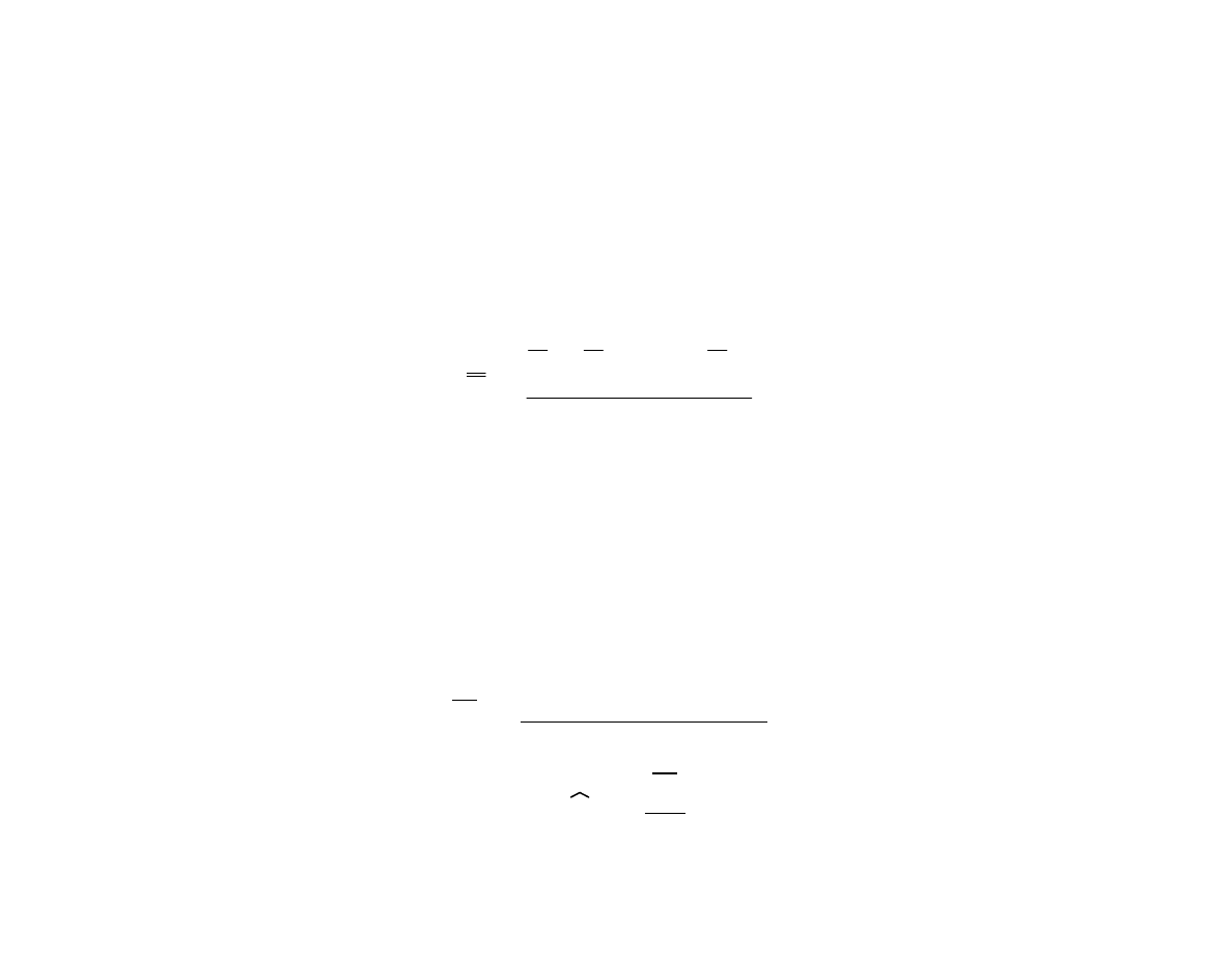
Statistical Basis for the Charts

standard deviation:

A normally distributed variable x with known

μ and σ, can be

controlled:

average:

x =

x

1

+x

2

+ ... +x

n

n

with µ ±

Z

α

2

σ

n

where

±

Z

α

2

is the distance from µ ( in # of

σ),

that would capture (1-

α)% of the normal.

s

2

=

n

Σ

i=1

(x

i

-µ)

2

n-1

~

σ

2

χ

(n-1)

2

n-1

with:

σ

2

χ

1

-

α

2

,(n-1)

2

n-1

< s

2

<

σ

2

χ

α

2

, (n-1)

2

n-1

where

χ

1

-

α

2

,(n-1)

2

and

χ

α

2

, (n-1)

2

are the

numbers that capture between them 1-α of the χ

(n-1)

2

distribution

Lecture 12: Control Charts for Variables

Spanos

EE290H F05

4

Control Chart for x and s

(with mean and variance known).

80

60

40

20

0

0.5

0.6

0.7

0.8

0.9

1.0

LCL 0.514 (-3

σ)

μ = 0.745

UCL 0.977 (+3

σ)

80

60

40

20

0

0.00

0.01

0.02

LCL 0.0003

UCL 0.0078

σ

2

= 0.0038

Lecture 12: Control Charts for Variables

Spanos

EE290H F05

5

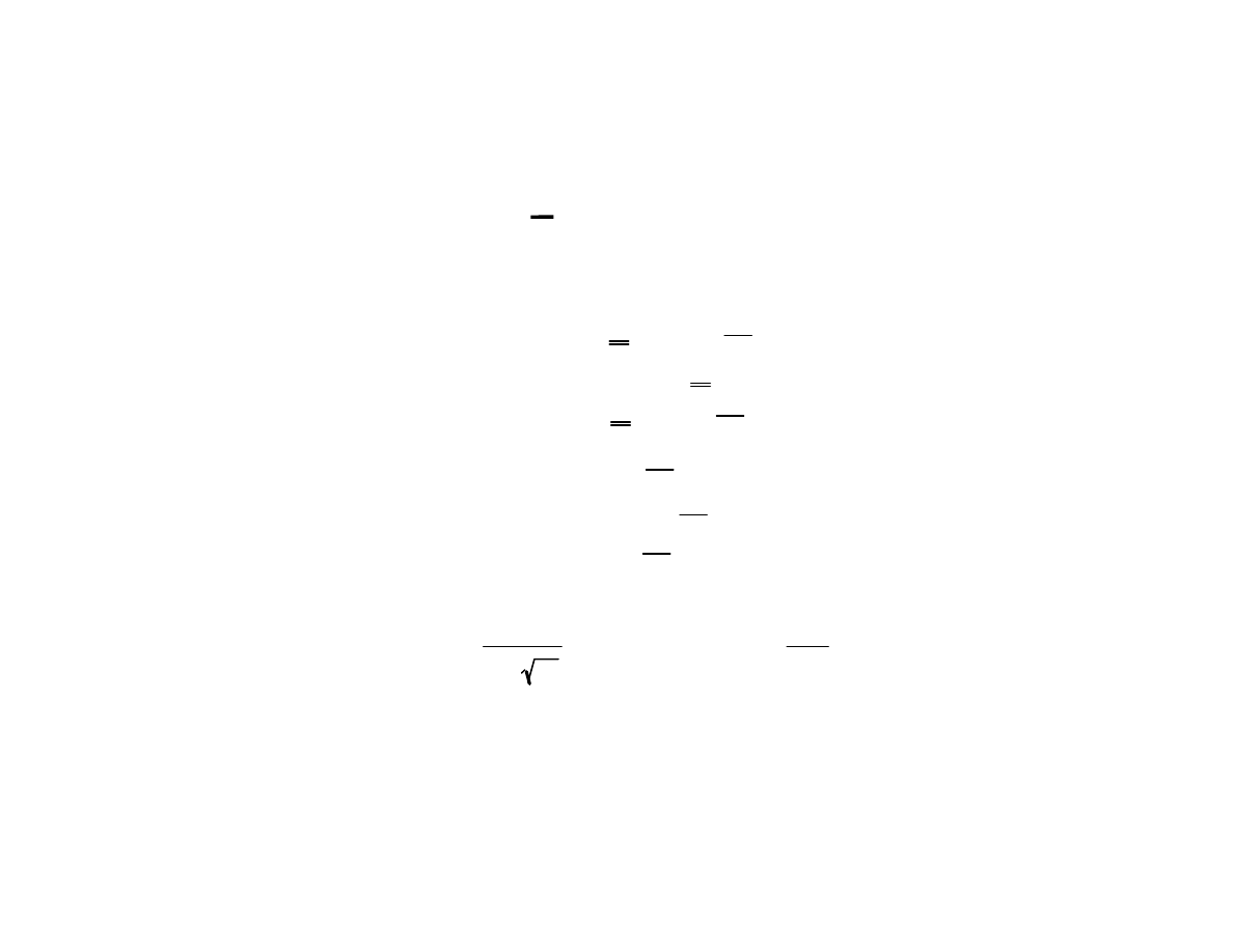
Statistical Basis for the Charts (cont.)

x =

x

1

+x

2

+ ... +x

m

m

R = x

max

- x

min

Range R is related to the sigma in terms of a constant
(depending on sample size) that is listed in statistical tables:

In practice we do not know the mean or the sigma. The
mean can be estimated by the grand average. If the sample
size is small, we can use the range to describe spread.

R =

R

1

+R

2

+ ... +R

m

m

σ = R

d

2

Lecture 12: Control Charts for Variables

Spanos

EE290H F05

6

Statistical Basis for the Charts (cont.)

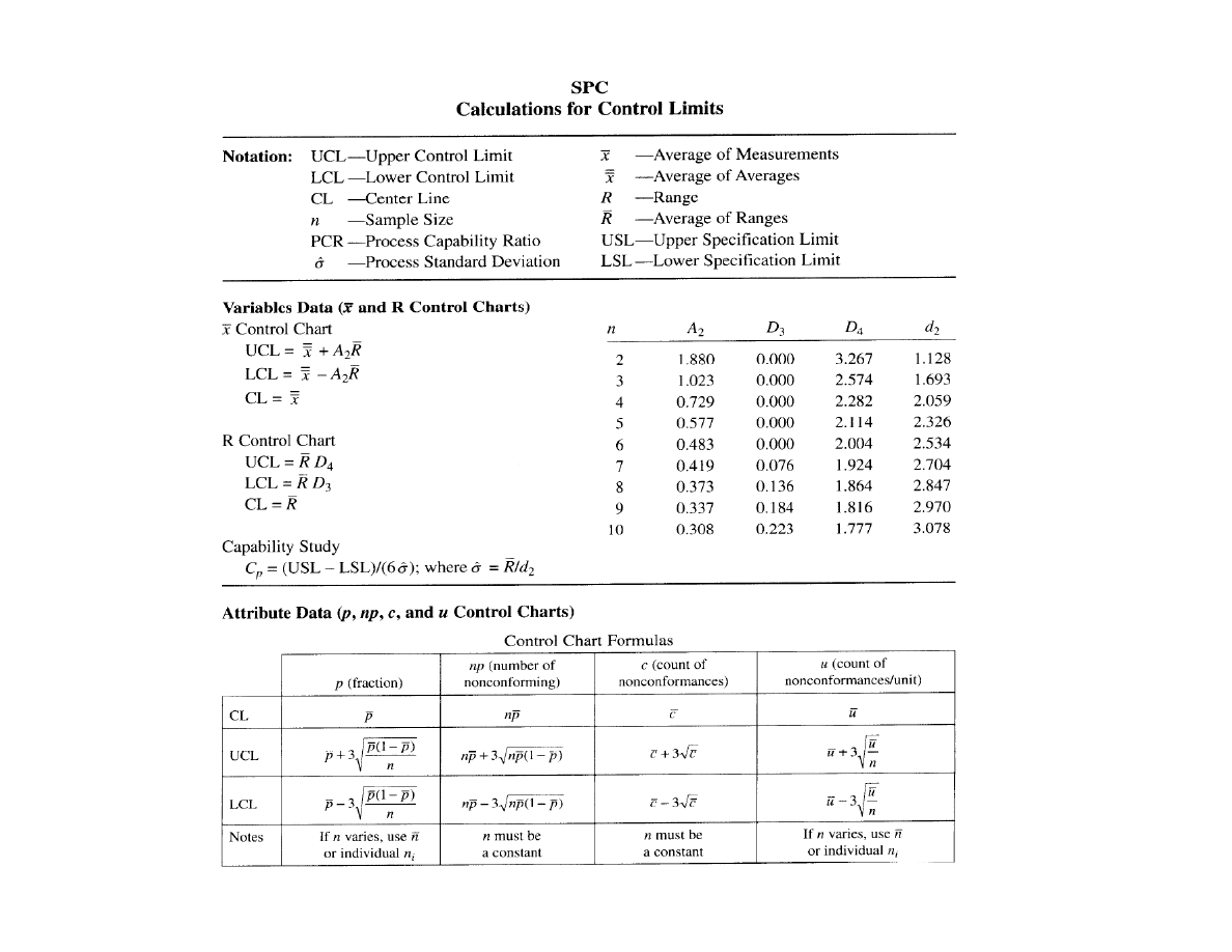
The control limits for the x-R chart are as follows:

UCL = x + A

2

R

center at x

LCL = x - A

2

R

UCL = RD

4

center at R

LCL = RD

3

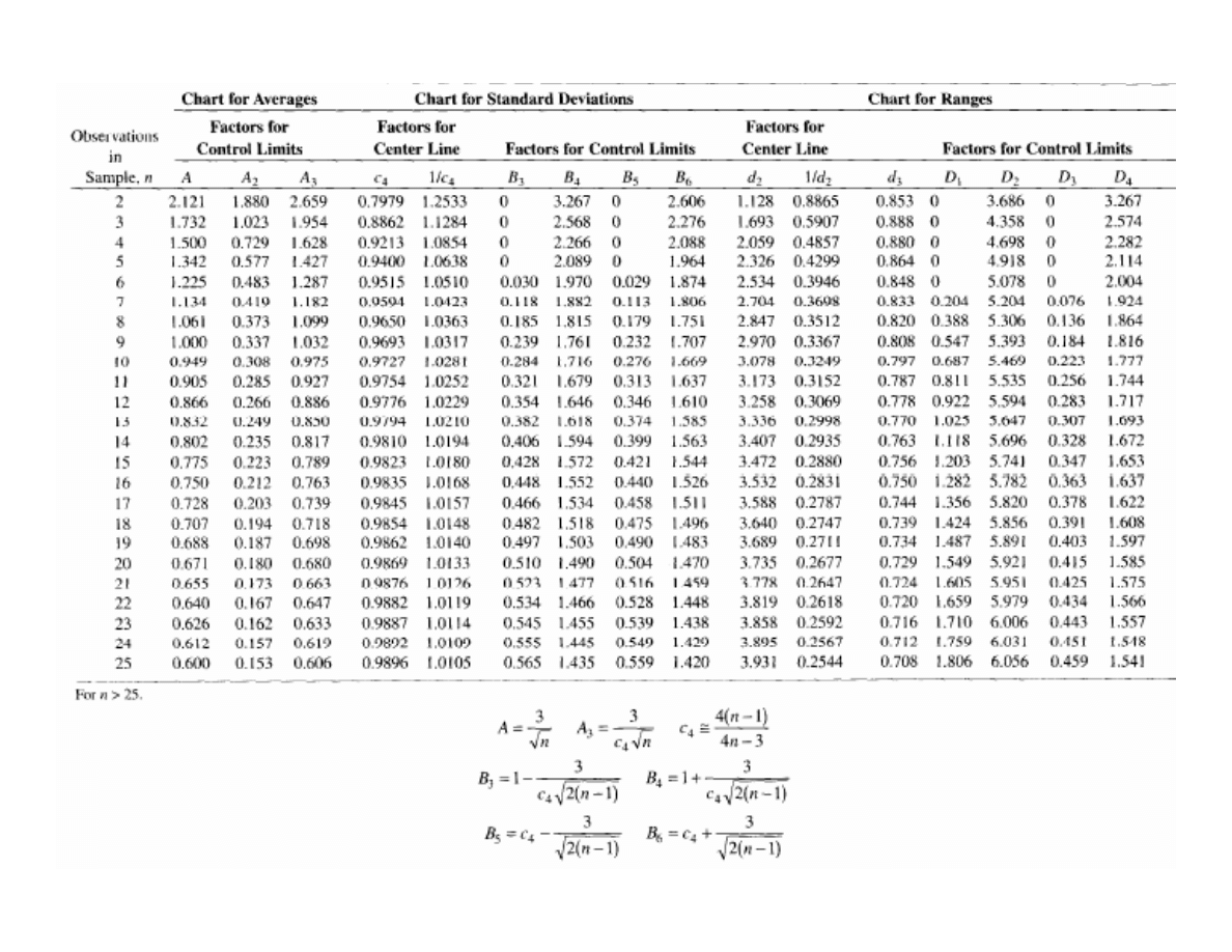
A

2

= 3

d

2

n

D

3,4

= 1±3

d

3

d

2

(d

2

and d

3

are tabulated constants that depend on n)

Lecture 12: Control Charts for Variables

Spanos

EE290H F05

7

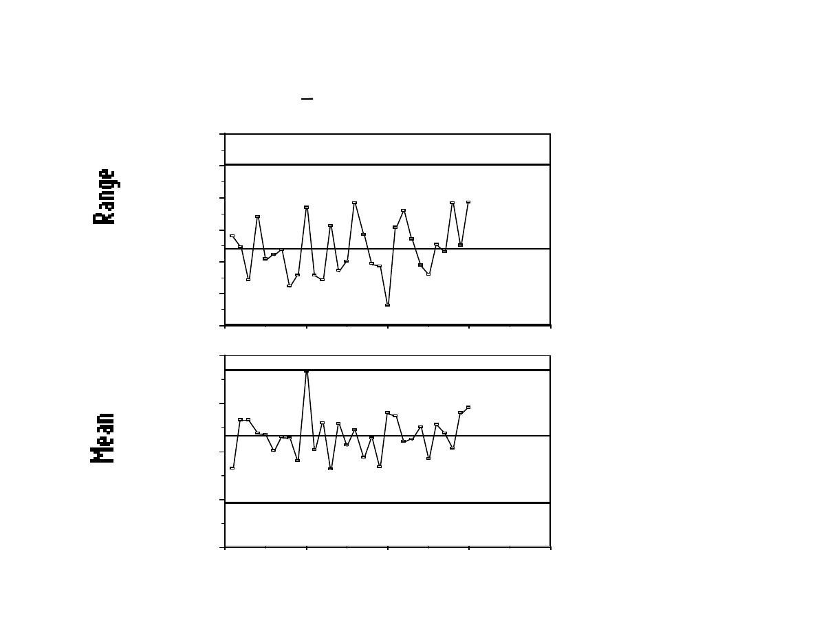
Range and Mean charts for Photoresist Control

Range

n=5 and from table, D

3

=0.0 and D

4

=2.11. Average Range is

239.4, so the range center line is 239.4, the LCL is 0.0 and
the UCL is 507.1. These control limits will give us the
equivalent of 3 sigma control. (

α = 0.0027).

x

The global average is 7832.9 and from table, A

2

is 0.577,

so LCL is 7694.5 and UCL is 7971.3. These control limits
will give us 3 sigma control. (

α = 0.0027).

Lecture 12: Control Charts for Variables

Spanos

EE290H F05

8

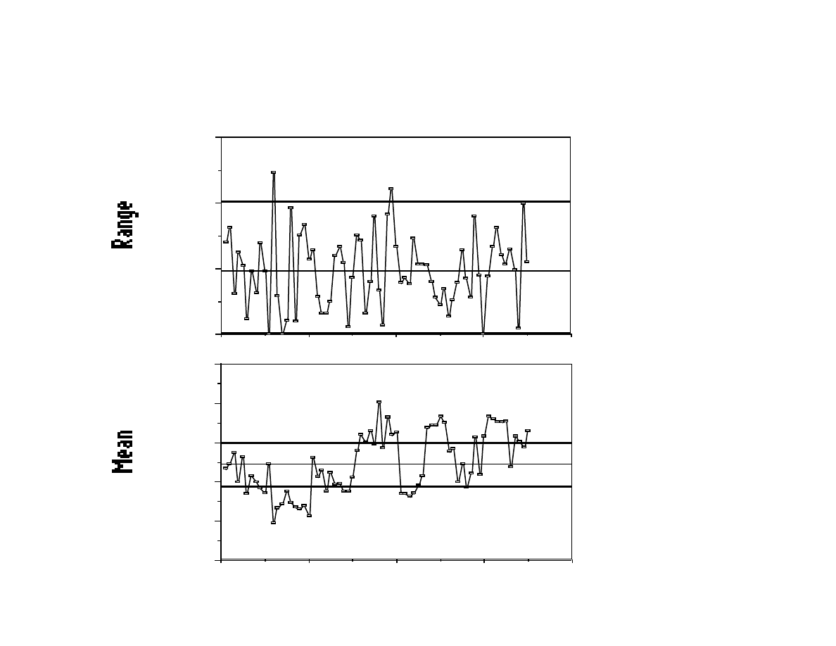
Example: Photoresist Coating (cont)

Range and x chart for all wafer groups.

0

100

200

300

400

500

600

LCL = 0.0

239.9

UCL = 507.1

40

30

20

10

0

7600

7700

7800

7900

8000

Wafer Groups

LCL = 7694.5

7832.9

UCL = 7971.3

Lecture 12: Control Charts for Variables

Spanos

EE290H F05

9

The Grouping of The Parameters is Crucial

Known as rational subgrouping, the choice of grouping is
very important.

In general, only random variation should be allowed within
the subgroup.

(i.e. grouping wafers within the boat of a diffusion tube is
inappropriate - gas depletion effect is systematic.)

The range of the appropriate group should be used to
estimate the variance of the process.

(i.e. the range across a lot should not be used to estimate
the variance of a parameter measured between lots - within
lot statistics are different from between lot statistics).

Lecture 12: Control Charts for Variables

Spanos

EE290H F05

10

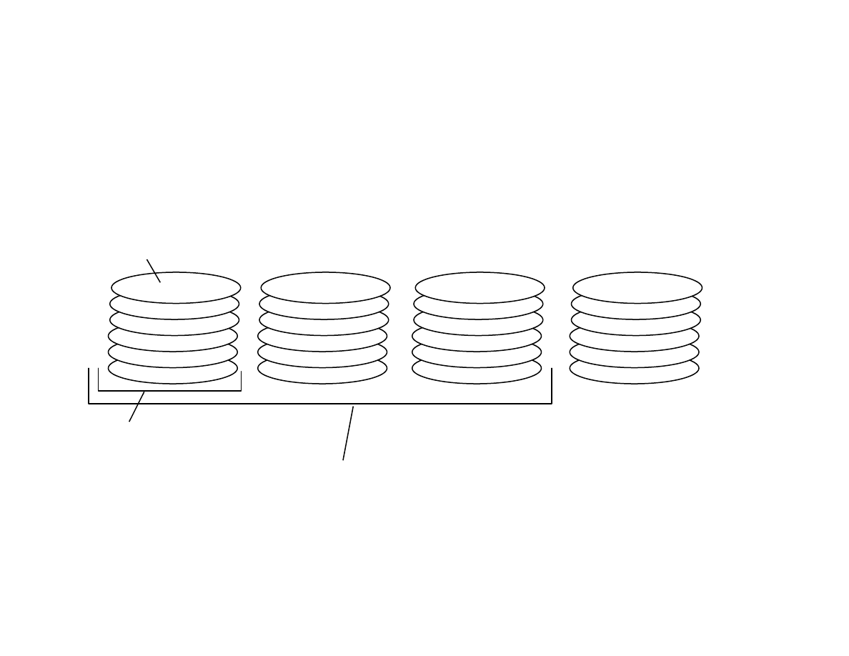
Rational Subgrouping

Rule of thumb: use only groups with IIND data, if possible.
(Independently, Identically, Normally Distributed).

Wafer

Lot

Batch

The natural grouping of semiconductor data might not lead
to IIND subgroups!

Lecture 12: Control Charts for Variables

Spanos

EE290H F05

11

Example: charts for line-width control

what is the problem?

what is the problem?

80

60

40

20

0

0.5

0.6

0.7

0.8

0.9

1.0

X chart, n=5, A2=0.577

Lot No

LCL 0.690

0.745

UCL 0.800

0.0

0.1

0.2

0.3

Range Chart, n=5 D3=0.0, D4=2.114

LCL 0.0

0.096

UCL 0.203

Lecture 12: Control Charts for Variables

Spanos

EE290H F05

12

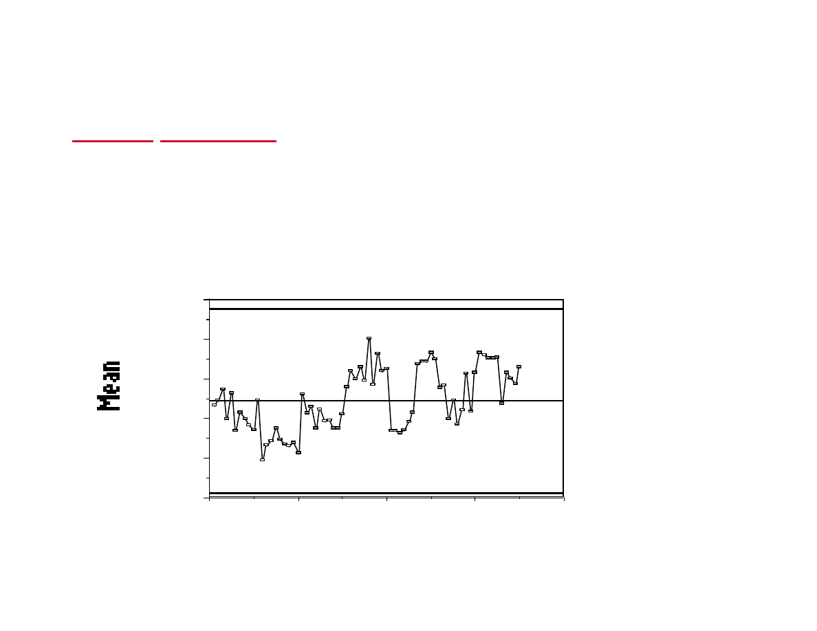
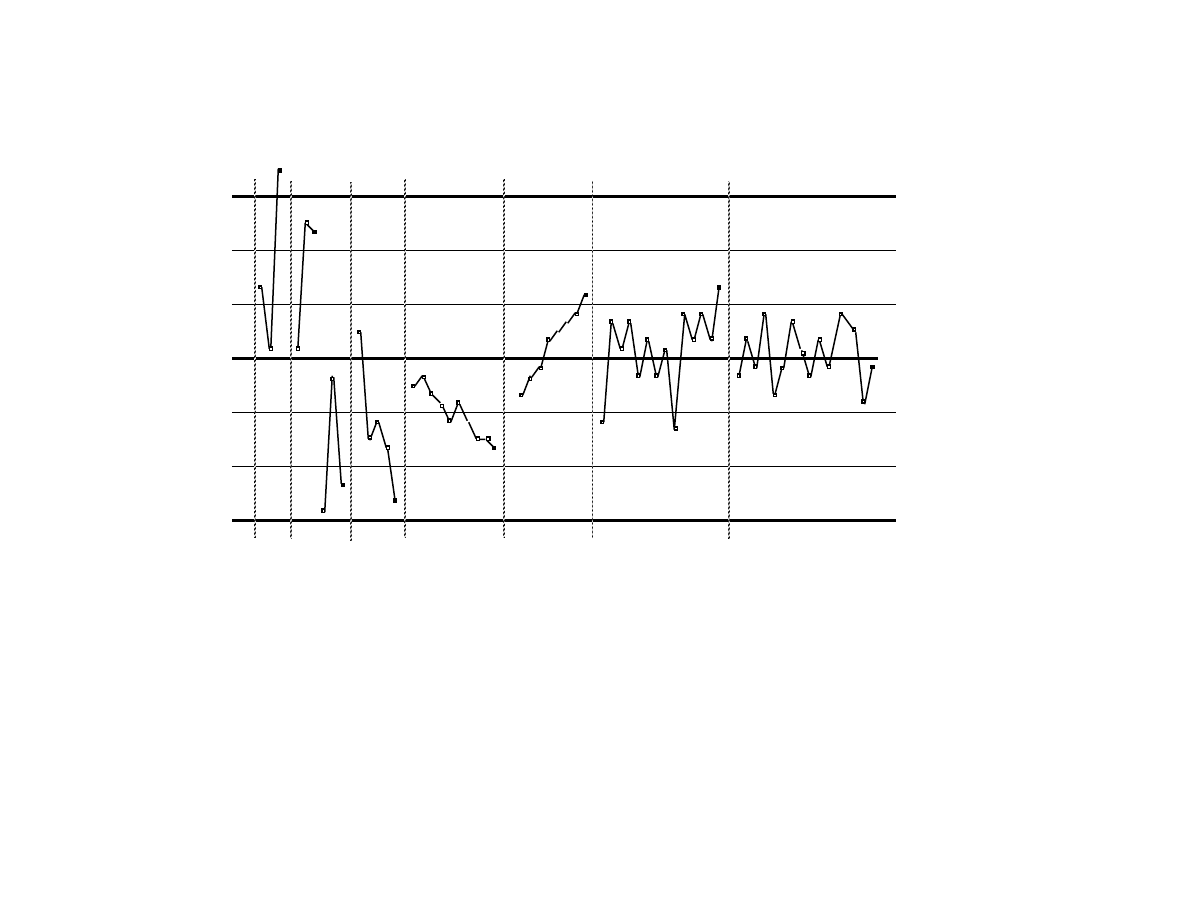
Rational Subgrouping (cont.)

Remember, we are using R to estimate the global sigma. The

rational subgroups

we chose might bias this estimation.

In this case, the within lot variation is much less than the
global variation.

If we estimate the sigma from the global range, we get:

If this looks too good, it might be because of the "mixture"
patterns in it!

80

60

40

20

0

0.5

0.6

0.7

0.8

0.9

1.0

X chart for Global Range

LCL 0.514

0.745

UCL 0.977

Lecture 12: Control Charts for Variables

Spanos

EE290H F05

13

Specification Limits vs. Control Limits

The specification limits of a process reflect our need. These
limits are set by the management as objectives.

The control limits of a process tell us what the process can
do when it is operating properly. These limits are set by the
quality of the machinery and the skills of the operators.

Process Capability is a figure of merit that tells us whether a
process is suitable for our manufacturing objectives.

Lecture 12: Control Charts for Variables

Spanos

EE290H F05

14

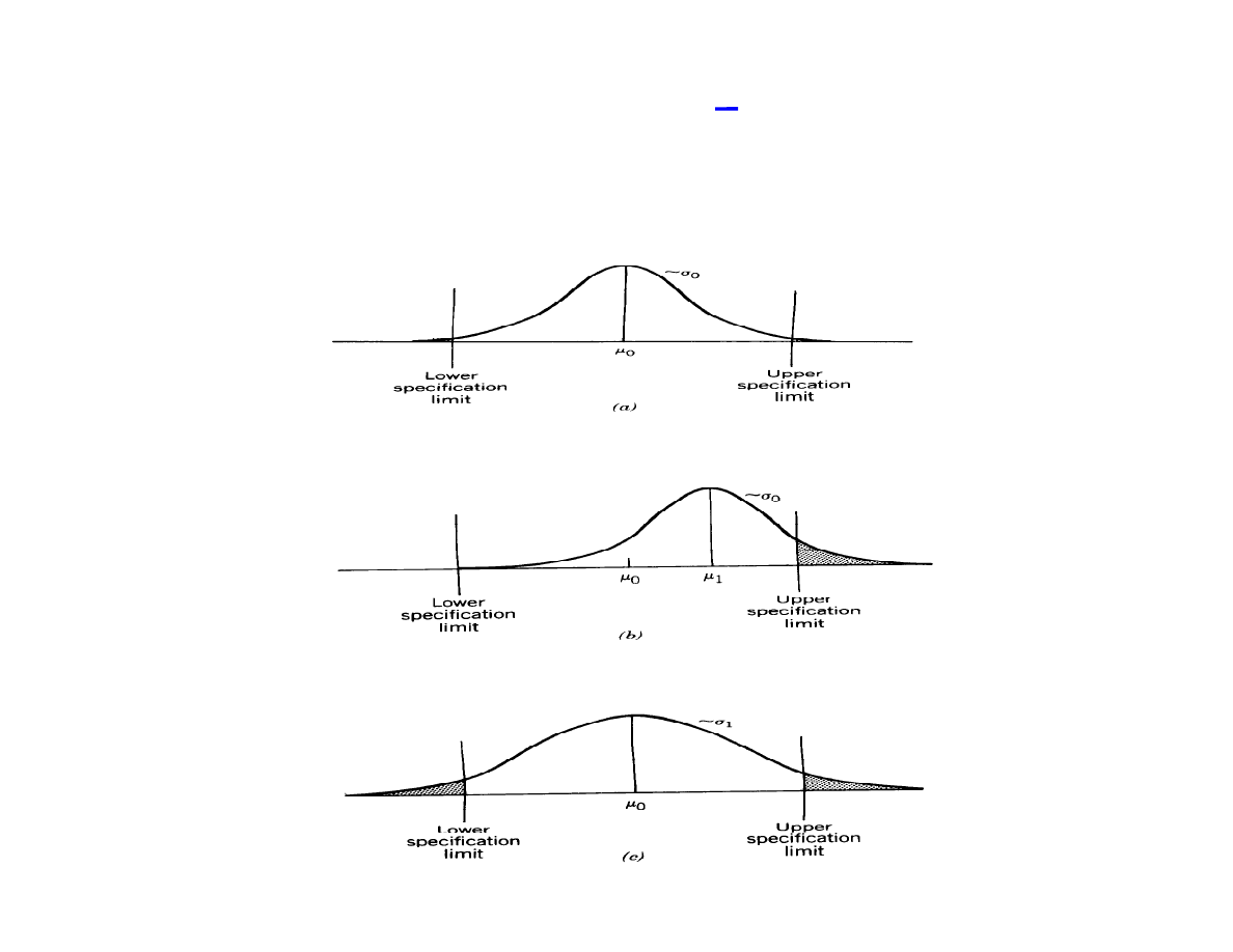
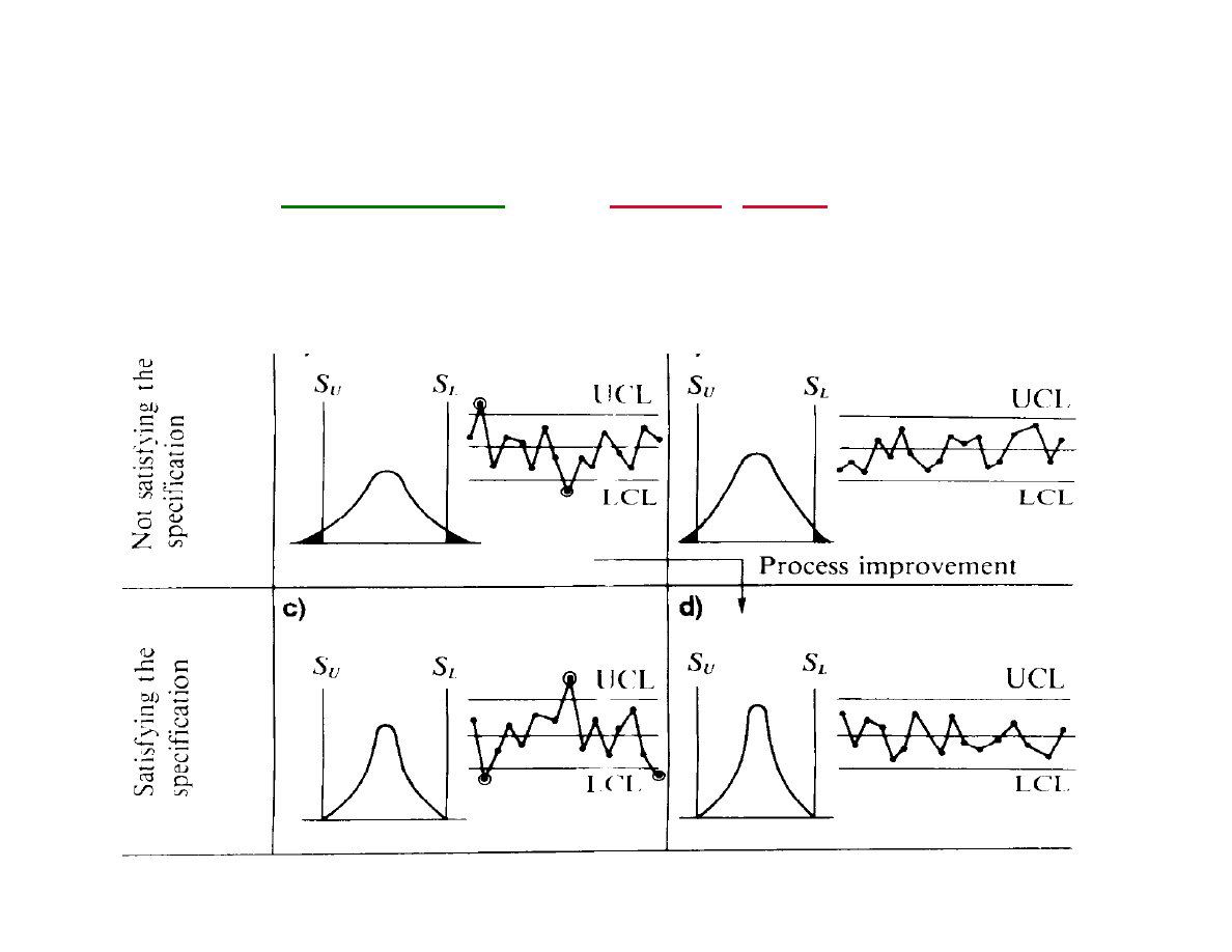
Process Capability

Figure 7.20 pp 139 Kume

Process

specifications

and

control limits

are, in general,

different concepts.

A process might be in control without meeting the specs, or
might be meeting the specs without being is control...

Lecture 12: Control Charts for Variables

Spanos

EE290H F05

15

Process Capability Estimation

Calculate what the process (when in control) can do and
compare it with specifications.

A control chart provides good estimates of

σ, so it can be

used for process capability evaluation.

Process Capability Ratio (PCR, C

P

)

C

p

= (USL-LSL) / 6

σ

Example

The line-width control data show a process capability of 1.08,
since the specs for DLN are .5 to 1.0 µm and

σ is .077.

The symbol C

PK

is used for the process capability when the

spec limits are not symmetrical around the process spread:

C

PK

= min { (USL-x)/3

σ, (x-LSL)/3σ }

Lecture 12: Control Charts for Variables

Spanos

EE290H F05

16

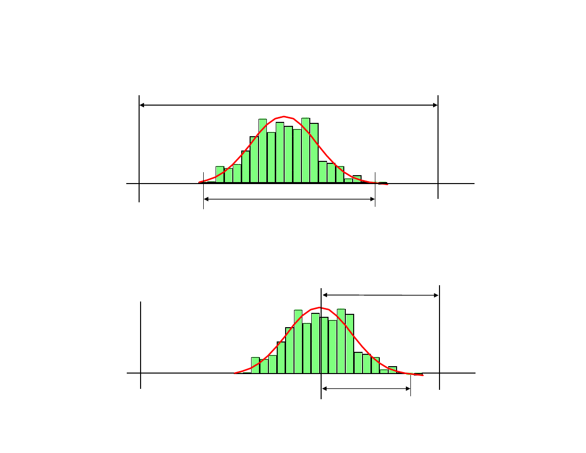
Process Capability (cont)

LSL

USL

6

σ

3

σ

LSL

USL

C

pk

= min { (USL-x)/3

σ, (x-LSL)/3σ }

C

p

= (USL-LSL) / 6

σ

Lecture 12: Control Charts for Variables

Spanos

EE290H F05

17

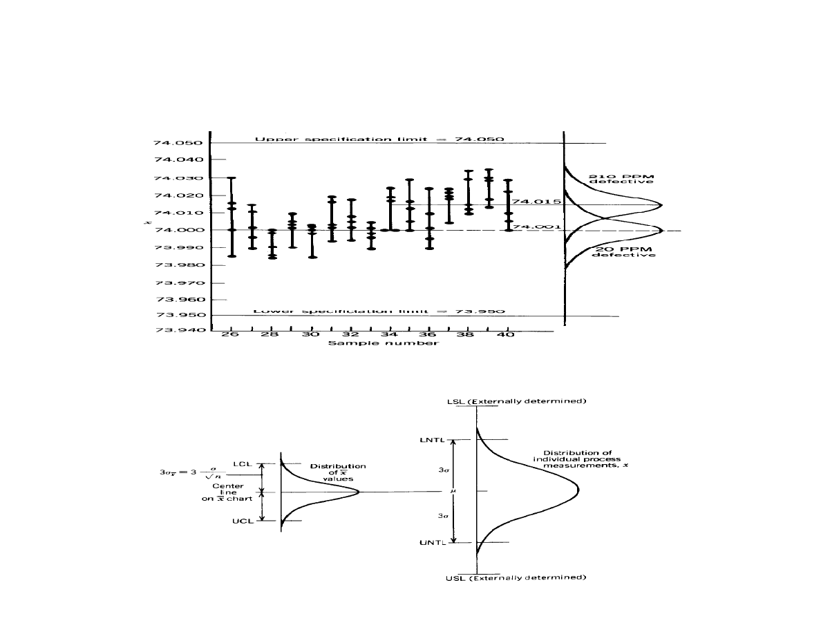
Never Mix Specification and Control Limits!

Relationship of natural tolerance, control and spec limits:

Only individuals should be plotted against the specs...

Lecture 12: Control Charts for Variables

Spanos

EE290H F05

18

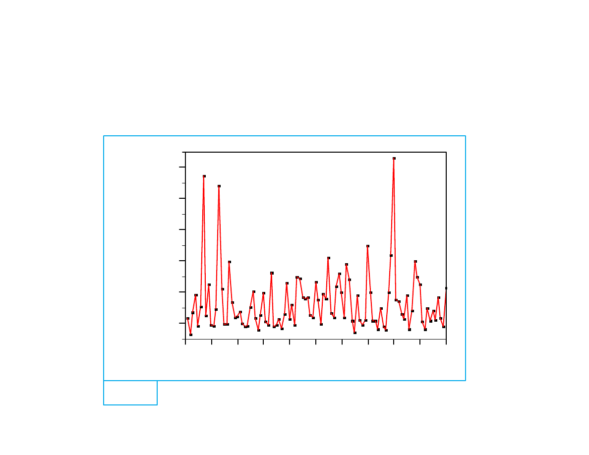
Never Attempt to Estimate Cp or Cpk

from small groups!

Plot of CP estimate, n=5 (true CP=0.67)

CP

0.5

1.0

1.5

2.0

2.5

3.0

0

10

20

30

40

50

60

70

80

90 100

CP

Lecture 12: Control Charts for Variables

Spanos

EE290H F05

19

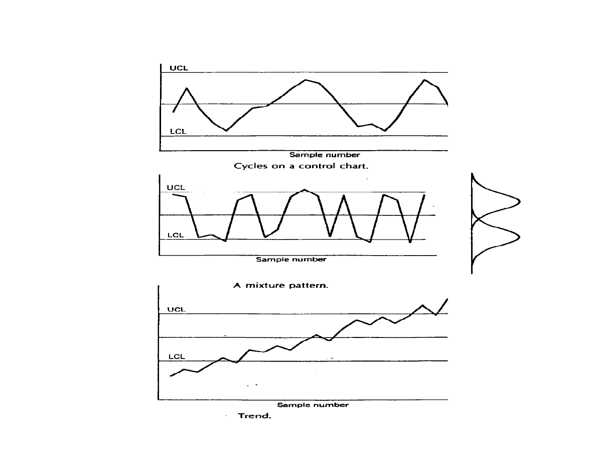
Special patterns in charts

While a point outside the control limits is a good indicator of
non-randomness, other patterns are possible:

• Cyclic (periodic signal)

• Mixtures (two or more sources)

• Shifts (abrupt change)

• Trends (gradual change)

• Stratification (variability too small)

Additional rules can be used to detect them. (Watch for an
increase in false alarm rates).

Lecture 12: Control Charts for Variables

Spanos

EE290H F05

20

Special Patterns

Lecture 12: Control Charts for Variables

Spanos

EE290H F05

21

The Western Electric Rules

UCL (+3

σ

)

LCL (-3

σ

)

Center
Line

A

B

A

C

B

C

1. Any point beyond 3s UCL or LCL.
2. 2/3 cons. points on same side, in A or beyond
3. 4/5 cons. points on same side, in B or beyond.
4. 9/9 cons. points on same side of center line.
5. 6/6 cons. points increasing or decreasing.
6. 14/14 cons. points alternating up and down.
7. 15/15 cons. points on either side in zone C.

1

2

3

4

5

6

7

Lecture 12: Control Charts for Variables

Spanos

EE290H F05

22

Robustness of the x-R control chart

X ~ N(µ,

σ

2

)

So far we have assumed that our process is fluctuating
according to a normal distribution:

This assumption is not important for the x chart (thanks to
the central limit theorem).

The R chart is much more sensitive to this assumption.

If the underlying distribution is not normal, watch for signs
of correlation between x and R.

Lecture 12: Control Charts for Variables

Spanos

EE290H F05

23

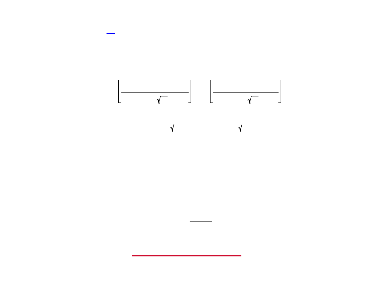
The x-R Operating Characteristic Function

also known as the

Average Run Length

β

m-1

(1 -

β)

ARL = 1

1 -

β

β = Φ UCL-(µ

o

+k

σ)

σ / n

-

Φ LCL-(µ

o

+k

σ)

σ / n

or, for 3

σ control linits:

β = Φ ( 3 - k n ) - Φ ( -3 - k n )

The probability that the shift will be detected on the m

th

sample is:

And the average number of samples that we need for
detecting this shift is:

What is the probability of not detecting a shift of

μ by k σ?

Lecture 12: Control Charts for Variables

Spanos

EE290H F05

24

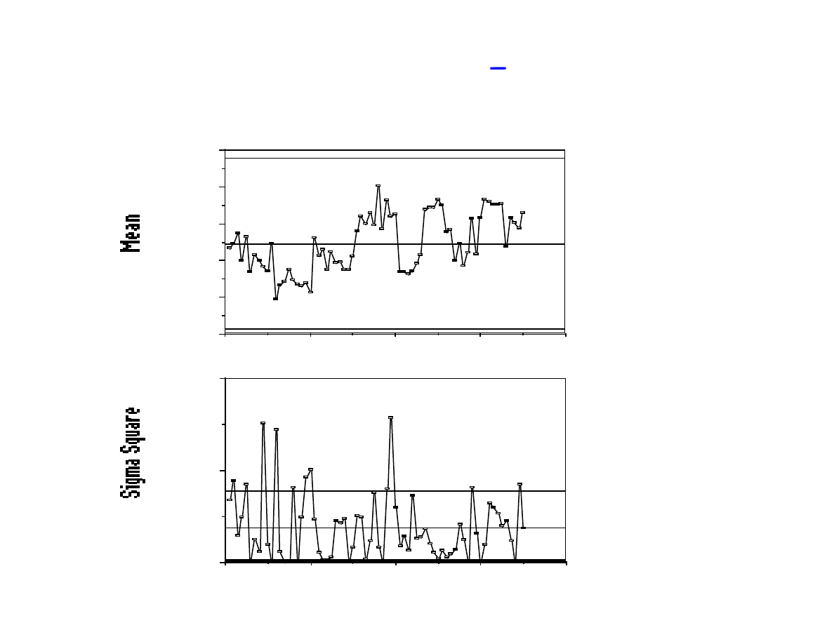
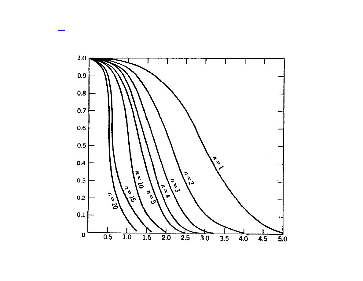
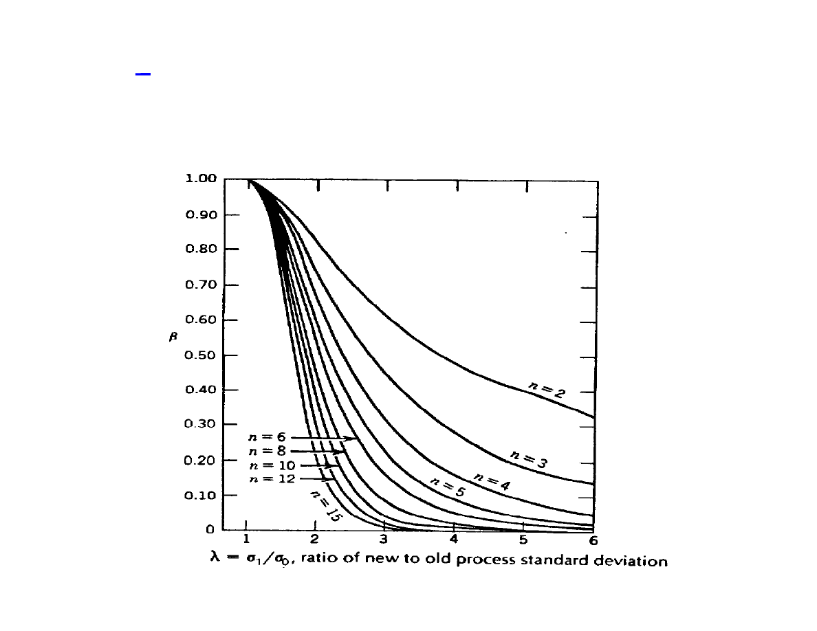
The x-R Operating Characteristic Function (cont.)

Lecture 12: Control Charts for Variables

Spanos

EE290H F05

25

The x-R Operating Characteristic Function (cont.)

The OC for the R part of the chart shows that it cannot catch
small shifts in sigma:

Lecture 12: Control Charts for Variables

Spanos

EE290H F05

26

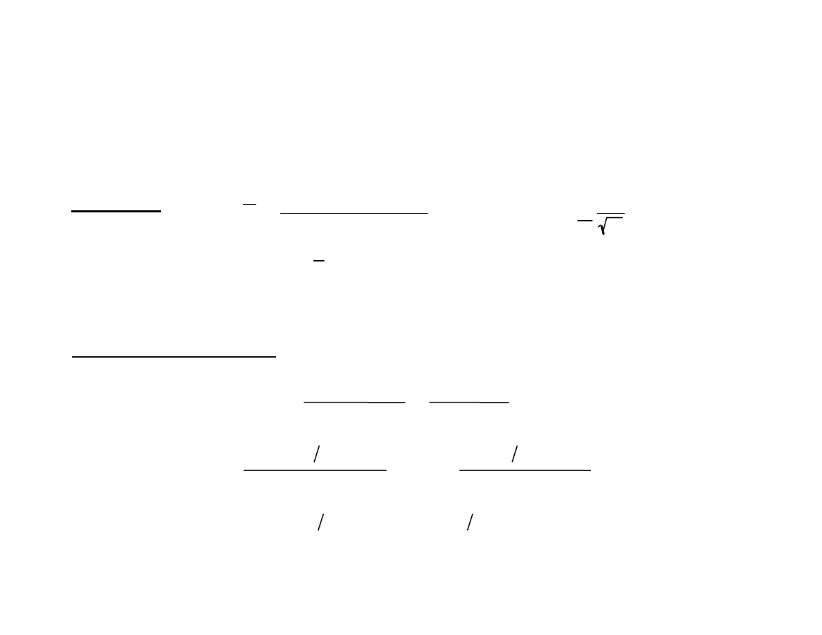
x - s control charts

s

2

=

n

Σ

i=1

(x

i

-x)

2

n-1

s =

1

m

m

Σ

i=1

s

i

and

s

C

4

unb. estim of sig

CL

s

= B

3,4

s B

3,4

= 1±

3

C

4

1-C

4

2

CL

x

= x ± A

3

s A

3

=

3

C

4

n

When n is larger (>10), then using the standard deviation s
gives better results. Although s

2

is a good, unbiased

estimator of the variance,

s is a biased estimator of sigma. A correction factor is a
function of n and can be found is tables. In summary:

Lecture 12: Control Charts for Variables

Spanos

EE290H F05

27

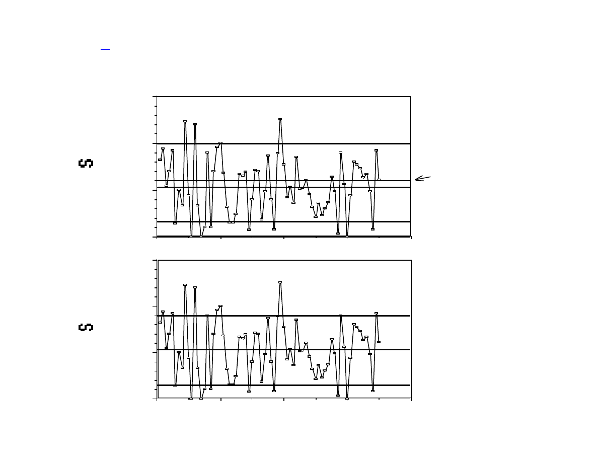
x and s Control Charts (when n is large)

0.00

0.05

0.10

0.15

S Chart, assuming sigma=0.06

B

5

=0.276, B

6

=1.669 for n=10

LCL 0.017

S 0.053

UCL 0.100

sigma

80

60

40

20

0

0.00

0.05

0.10

0.15

S Chart, no standard

B

3

=0.281, B

4

=1.716 for n=10

Lot No

LCL 0.015

S 0.053

UCL 0.091

Lecture 12: Control Charts for Variables

Spanos

EE290H F05

28

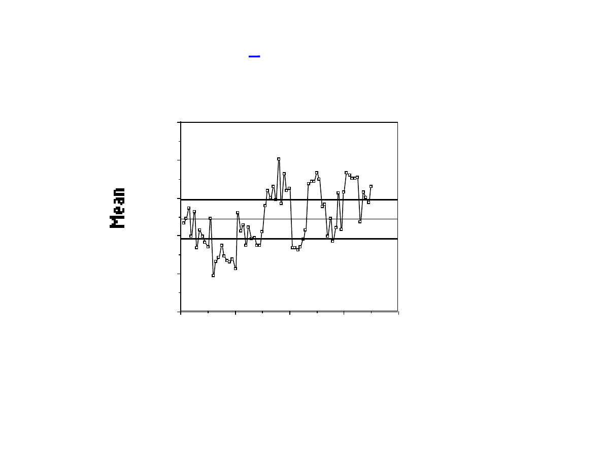
The control limits for x can now be calculated from s.

80

60

40

20

0

0.5

0.6

0.7

0.8

0.9

1.0

S=0.053, n=10, A

3

=0.975

Lot No

LCL 0.69

0.75

UCL 0.80

Lecture 12: Control Charts for Variables

Spanos

EE290H F05

29

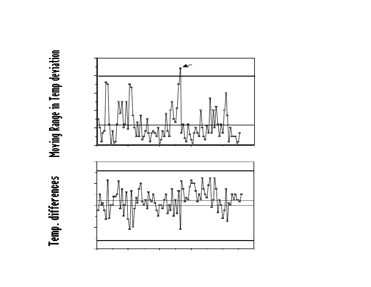
Control Charts for Individual Units

Moving Range chart for Temp. Control:

0

1

2

3

4

5

Moving Range Graph, n=2, D

3

=0.0, D

4

=3.267

LCL 0.0

1.16

UCL 3.92

100

80

60

40

20

0

-4

-2

0

2

4

Temp Samples, n=2, d

2

=1.128

Time

LCL -3.19e+0

4.5e-1

UCL 3.2e+0

Lecture 12: Control Charts for Variables

Spanos

EE290H F05

30

Questions Most Frequently Asked

Q How many points are needed to establish control limits?

A Typically 20-30 in-control points will do.

Q How do I know whether points are in-control if limits have
not been set?

A Out-of-control points should be: a) explained and
excluded. b) left in the graph if cannot be explained.

When done, we should have about 1/ARL unexplained out-
of-control points (for 3

σ control ~1/370 samples.) These

points are accepted as false alarms.

Q How often limits must be recalculated?

A Every time it is obvious from the chart that the process
has reached a new, acceptable state of statistical control.

Lecture 12: Control Charts for Variables

Spanos

EE290H F05

31

Choosing the proper control chart

Variables

• new process or product
• old process with chronic trouble
• diagnostic purposes
• destructive testing
• very tight specs
• decide adjustments

Attributes
• reduce process fallout
• multiple step process evaluation
• cannot measure variables
• historical summation of the process

Individuals
• physically difficult to group
• full testing or auto measurements
• data rate too slow

Lecture 12: Control Charts for Variables

Spanos

EE290H F05

32

Summary, so far

• Continuous variables need two (2) charts:

– chart monitoring the mean
– chart monitoring the spread

• Rational subgrouping must be done correctly.
• Charts are using Control Limits - Spec limits are very

different (conceptually and numerically).

• The concept of process capability brings the two sets of

limits together.

• A chart is a hypothesis test. It suffers from type I and

type II errors.

• Violating the control limits is just one type of alarm, out of

many.

Lecture 12: Control Charts for Variables

Spanos

EE290H F05

33

Lecture 12: Control Charts for Variables

Spanos

EE290H F05

34

Intro to SQC 5

th

Edition,

D. Montgomery