Lecture 15: Multivariate and Model-based SPC

Spanos

EE290H F05

1

Multivariate Control and Model-Based SPC

T

2

, evolutionary operation, regression

chart.

Lecture 15: Multivariate and Model-based SPC

Spanos

EE290H F05

2

Multivariate Control

t =

(x - µ

0

)

s

x

=

(x - µ

0

)

s

2

n

~ t(n-1)

α' = 1 - (1 - α)

p

P{all in control} = (1 -

α)

p

Often, many variables must be controlled at the same time.
Controlling p independent parameters with parallel charts:

If the parameters are correlated, the type I (false alarms)
and type II (missed alarms) rates change.

We need is a single comparison test for many variables. In
one dimension, this test is based on the student t statistic:

Lecture 15: Multivariate and Model-based SPC

Spanos

EE290H F05

3

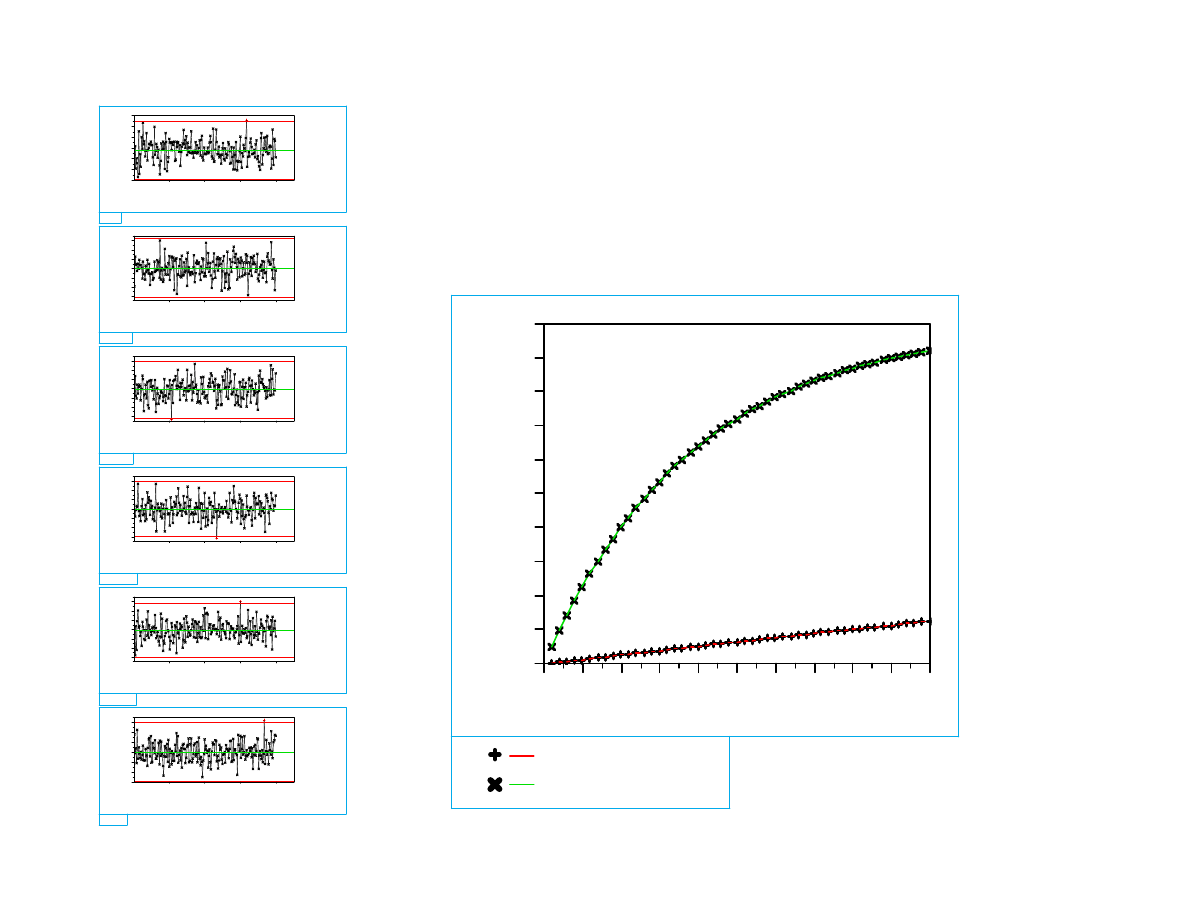
Monitoring Multiple Un-correlated

Variables

IR Charts

CD

-3

-2

-1

0

1

2

3

1

50

100

150

200

Avg=-0.2

LCL=-2.9

UCL=2.5

CD

Thi

ck

-3

-2

-1

0

1

2

3

50

100

150

200

Avg=0.1

LCL=-3.2

UCL=3.3

Thick

A

ngl

e

-3

-2

-1

0

1

2

3

1

50

100

150

200

Avg=-0.1

LCL=-3.1

UCL=3.0

Angle

X-

m

iss

-3

-2

-1

0

1

2

3

1

50

100

150

200

Avg=0.0

LCL=-3.0

UCL=3.0

X-miss

Y-

M

iss

-3

-2

-1

0

1

2

3

1

50

100

150

200

Avg=-0.1

LCL=-3.0

UCL=2.9

Y-Miss

Re

fl

-3

-2

-1

0

1

2

3

1

50

100

150

200

Avg=0.0

LCL=-2.9

UCL=3.0

Refl

Type I Error vs Number of Variables

0.0

0.1

0.2

0.3

0.4

0.5

0.6

0.7

0.8

0.9

1.0

0

5

10 15 20 25 30 35 40 45 50

type I, 3sigma
type I, 0.05

Lecture 15: Multivariate and Model-based SPC

Spanos

EE290H F05

4

Multivariate Control (cont.)

T

2

= n ( x - x)' S

-1

(x - x)

T

α, p, n - 1

2

=

p(n - 1)

n - p F

α, p, n - p

with x =

x

1

x

2

...

x

p

, x =

x

1

x

2

...

x

p

S is the covariance matrix, x are the means for the last
sample and x the global means. We get an alarm when the
T

2

exceeds a critical value (set by the F-statistic).

To compare p mean values to an equal number of targets we
use the T

2

statistic:

Lecture 15: Multivariate and Model-based SPC

Spanos

EE290H F05

5

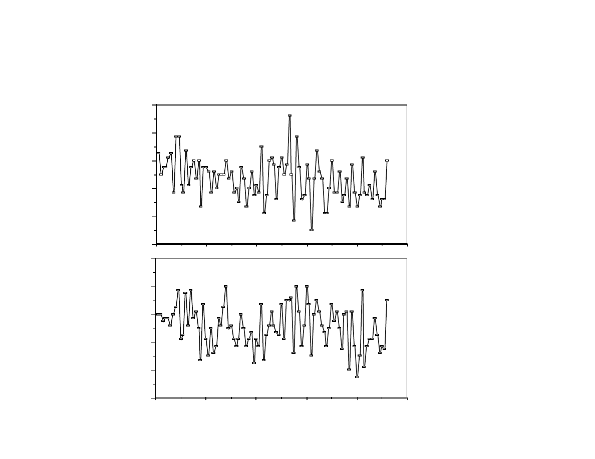
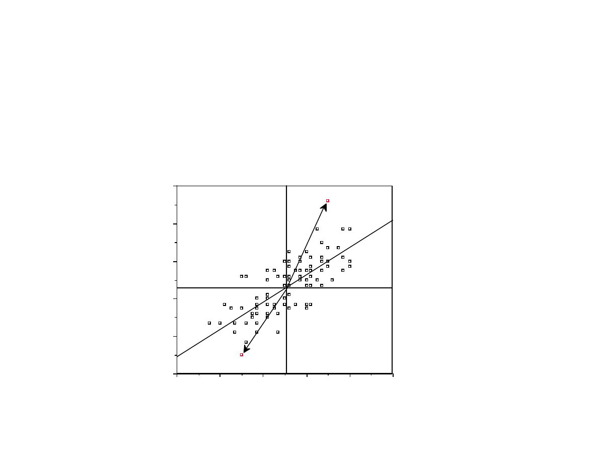
Example: Center and left temps are correlated

600

602

604

606

608

610

100

80

60

40

20

0

600

602

604

606

608

610

left

center

Lecture 15: Multivariate and Model-based SPC

Spanos

EE290H F05

6

Examining the two Variables Together

Correlations

Variable
Cent Temp
Left Temp

Cent Temp

1.0000
0.6094

Left Temp

0.6094
1.0000

602

602.5

603

603.5

604

604.5

605

605.5

606

606.5

607

607.5

608

601

603

605

607

609

Lecture 15: Multivariate and Model-based SPC

Spanos

EE290H F05

7

Example (cont.)

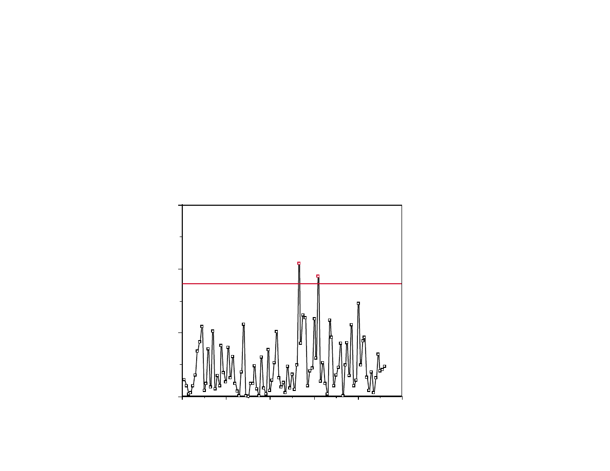
α = 0.05

Since left and center are correlated, with estimated

σ =1.15,

ρ=0.61, their deviation from the target 605 can be
determined by a single plot:

100

80

60

40

20

0

0

10

20

30

T

2

Lecture 15: Multivariate and Model-based SPC

Spanos

EE290H F05

8

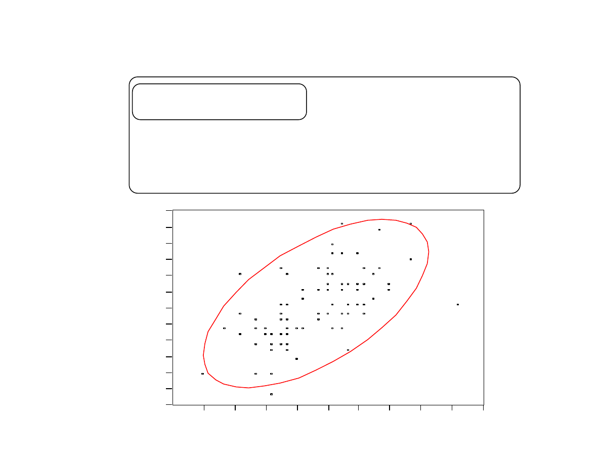
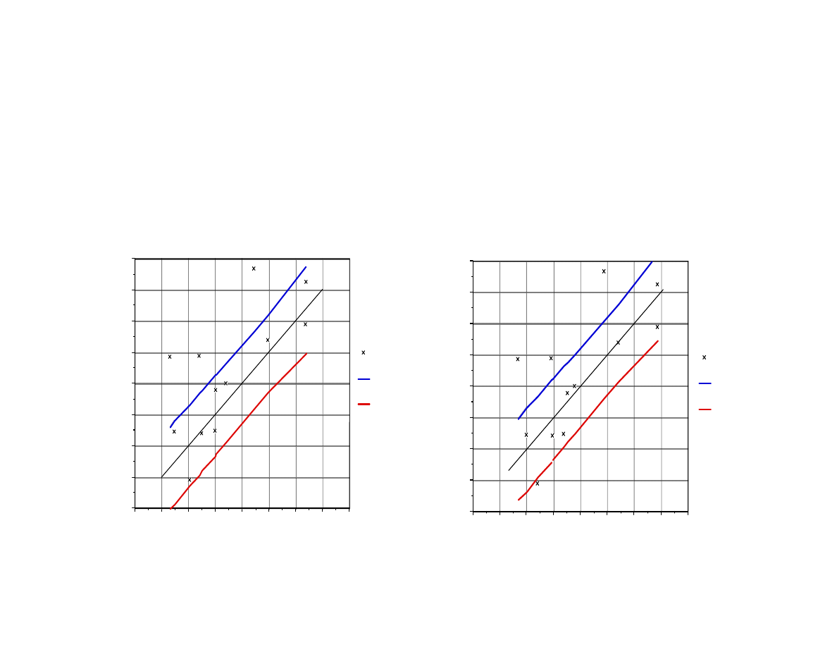
Example (cont.)

For two parameters, another graphical
representation is possible:

610

608

606

604

602

600

600

602

604

606

608

610

center

left

Lecture 15: Multivariate and Model-based SPC

Spanos

EE290H F05

9

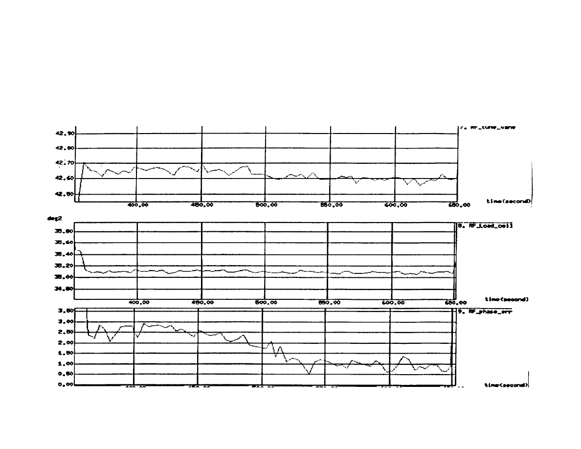
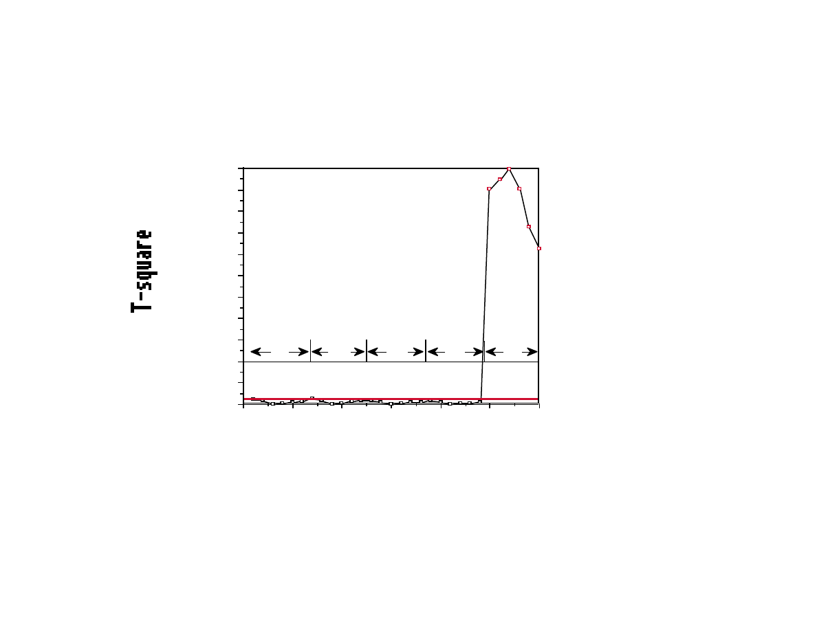
Example - Multivariate Control of Plasma Etch

Haifang's Screen Dump

Five strongly correlated parameters* can be collected during
the process:

*

Tune vane, load coil, phase error, plasma imp. and peak-to-peak voltage.

Lecture 15: Multivariate and Model-based SPC

Spanos

EE290H F05

10

Example - Multivariate SPC of Plasma Etch (cont.)

The first 24 samples were recorded during the etching of 4
"clean" wafers. The last 6 are out of control and they were
recorded during the etching of a "dirty" wafer.

30

25

20

15

10

5

0

0

200

400

600

800

1000

1200

1400

1600

1800

2000

2200

UCL 55.00

1

2

3

4

5

Lecture 15: Multivariate and Model-based SPC

Spanos

EE290H F05

11

Evolutionary Operation - An SPC/DOE Application

y = f (x

1

, x

2

) + e

and assume the following approximate model:

y - a x

1

+ b x

2

+ c x

1

x

2

If we knew a, b, and c, we would know how to change the
process in order to bring y closer to the specifications.

Of course this model will only be applicable for a narrow
range of the input parameters.

A process can be optimized on-line, by inducing small
changes and accepting the ones that improve its quality.

EVOP can be seen as an on-line application of designed
experiments.

Example: Assume a two-parameter process:

Lecture 15: Multivariate and Model-based SPC

Spanos

EE290H F05

12

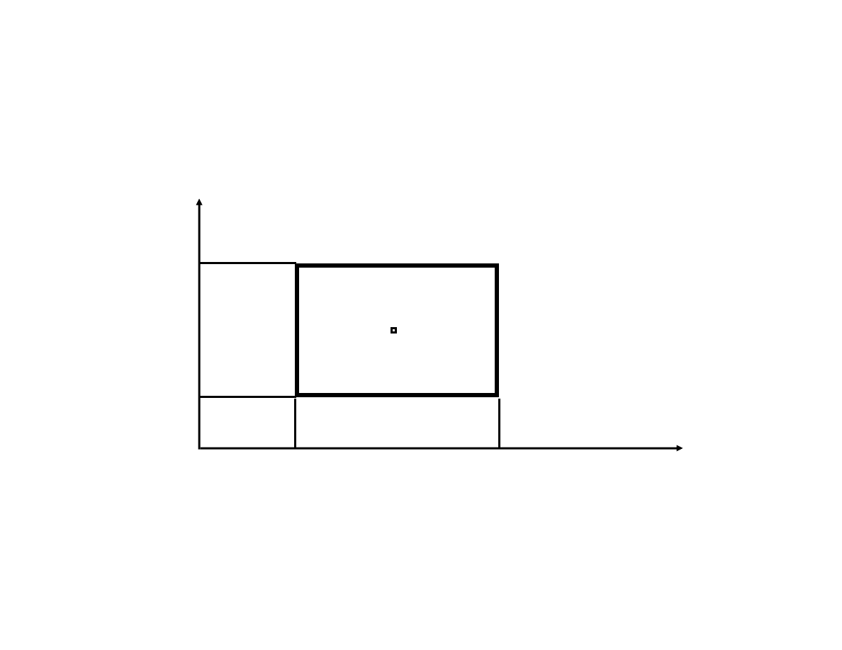
Evolutionary Operation (cont.)

design a 2

2

factorial experiment

x

2

x

1

y

5

y

3

y

2

y

4

y

1

L

H

L

H

+1

-1

+1

-1

(Note that x

1

and x

2

are scaled so that they take the

values -1, +1, at the edges of the experiment).

Lecture 15: Multivariate and Model-based SPC

Spanos

EE290H F05

13

Evolutionary Operation (cont.)

x

2

x

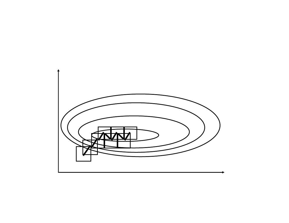
1

The process terminates when I find a box whose corners are
no better than its center.

Once the effects are known, choose the best corner of the
box and start a new experiment around it:

Lecture 15: Multivariate and Model-based SPC

Spanos

EE290H F05

14

Evolutionary Operation (cont.)

The values of a, b and c (or the respective "effects" and
"interactions") can be estimated:

This calculation is repeated for n-cycles until one of the
effects emerges as a significant factor.

a = Eff

x1

= 1

2

[(y

3

+y

4

) - (y

2

+y

5

)]

b = Eff

x2

= 1

2

[(y

3

+y

5

) - (y

2

+y

4

)]

c = Int

x1x2

= 1

2

[y

2

+y

3

- (y

4

+y

5

)]

Lecture 15: Multivariate and Model-based SPC

Spanos

EE290H F05

15

Evolutionary Operation (cont.)

+/-

+/-

N ( 0,

σ

2

n

n - 1

)

2

n

s

1.78

n

s

To decide whether an effect is significant, we need a good
estimate of the process sigma.

The sigma of the process can be estimated from the
difference of the last average and the new value at each of
the experimental points. This value is distributed as:

The 95% confidence interval of each effect is:

and of the change-in-mean effect is:

Lecture 15: Multivariate and Model-based SPC

Spanos

EE290H F05

16

Example - Use EVOP on a cleaning solution

conc. effect =

1
2

[(y

3

+y

4

) - (y

2

+y

5

)] = -0.025

temp. effect =

1
2

[(y

3

+y

5

) - (y

2

+y

4

)] = -3.800

interaction =

1
2

[y

2

+y

3

- (y

4

+y

5

)] = 4.825

chng in mean =

1
5

[y

2

+y

3

+y

4

+y

5

- 4y

1

] = -0.540

The yield from the first 4 cycles of a chem. process is shown
below. The variables are % conc. (x

1

) at 30 (L), 31 (M), 32 (H)

and temp. (x

2

) at 140 (L), 142 (M), 144 F (H).

Cycle Y

1 M-M

Y

2 L-L

Y

3 H-H

Y

4 H-L

Y

5 L-H

1

60.7

69.8

60.2

64.2

57.5

2

69.1

62.8

62.5

64.6

58.3

3

66.6

69.1

69.0

62.3

61.1

4

60.5

69.8

64.5

61.0

60.1

avg Y

64.2

67.9

64.1

63.0

59.3

Lecture 15: Multivariate and Model-based SPC

Spanos

EE290H F05

17

Example - EVOP on a cleaning solution (cont.)

+/- 2

σ / n = +/- 2.787

Take range of ( y

i

j

- y

i

j-1

) for i = 1,2,3,4,5

ave rage for j = 2,3,4 R

D

= 7.53

and

R

D

d

2

=

σ n/(n-1) , i.e. σ =2.787

So, temperature and interaction are significant. Their signs
dictate moving to point 2 (L-L).

The 95% confidence limits for concentration, temperature
and their interaction are:

We use the range of consecutive differences in order to
estimate the sigma of the process:

Lecture 15: Multivariate and Model-based SPC

Spanos

EE290H F05

18

EVOP Monitoring in the Fab

Lecture 15: Multivariate and Model-based SPC

Spanos

EE290H F05

19

Regression Chart - Model Based SPC

In typical SPC, we try to establish that certain process
responses stay on target.

What happens if there is one assignable cause that we know
and we can quantify?

If, for example, the deposition rate of poly is a function of the
time since the last tube cleaning, it will never be "in control".

In cases like this, we build a regression model of the
response vs the known effect, and we try to establish that the
regression model remains valid throughout the operation.

Limits around the regression line are set according to the
prediction error of the model.

A t-statistic is used to update the model whenever necessary.

Lecture 15: Multivariate and Model-based SPC

Spanos

EE290H F05

20

Regression chart (cont.)

20

10

0

200

400

600

800

1000

1200

1400

Polysilicon Deposition Rate

Sample Count

LCL 245.51

797.24

UCL 1348.96

30

20

10

0

500

600

700

800

900

1000

1100

Regression Chart

# of runs after clean

2

σ

Lecture 15: Multivariate and Model-based SPC

Spanos

EE290H F05

21

Regression Chart (cont.)

• The regression chart can be generalized for complex

equipment models.

• An empirical model is built to describe the changing

aspects of the process.

• The difference between prediction and observation

can be used as the control statistic

• If the control statistic becomes consistently different

than zero, its value can be used to update the model.

Lecture 15: Multivariate and Model-based SPC

Spanos

EE290H F05

22

Model Test and Adaptation

LPCVD Model

ln(Ro) = A + B ln (P) + C(1/T) + D (1/Q)

After substitution, the equation used is:

Y = A + Bx

B

+ Cx

C

+ Dx

D

Control Limits: Y +/- (t * s)

Cumulative

t =

(Y

i

-y

i

)

s

y

Σ

i=1

n

Lecture 15: Multivariate and Model-based SPC

Spanos

EE290H F05

23

Regression Chart (Example)

5.6

5.5

5.4

5.3

5.2

5.1

5.0

4.9

4.8

4.8

4.9

5.0

5.1

5.2

5.3

5.4

5.5

5.6

5.7

5.8

5.9

6.0

Actual
Rate
UCL

LCL

Model Rate [ln(Å/min)]

A

c

tual Rate [ln(Å/min)]

5.6

5.5

5.4

5.3

5.2

5.1

5.0

4.9

4.8

4.8

4.9

5.0

5.1

5.2

5.3

5.4

5.5

5.6

Actual
Rate

UCL
LCL

Model Rate [ln(Å/min)]

A

c

tual Rate [ln(Å/min)]

Lecture 15: Multivariate and Model-based SPC

Spanos

EE290H F05

24

Regression Chart (Example)

5.6

5.5

5.4

5.3

5.2

5.1

5.0

4.9

4.8

4.8

4.9

5.0

5.1

5.2

5.3

5.4

5.5

5.6

Actual Rate

UCL

LCL

Model Rate [ln(Å/min)]

Ac

tua

l Ra

te

[ln(Å/min)]

5.6

5.5

5.4

5.3

5.2

5.1

5.0

4.9

4.8

4.8

4.9

5.0

5.1

5.2

5.3

5.4

5.5

5.6

Actual Rate

Revised UCL

Revised LCL

Revised Model Rate [ln(Å/min)]

Actual Rate [ln(Å/min)]

Outdated Model

Updated Model

Lecture 15: Multivariate and Model-based SPC

Spanos

EE290H F05

25

Summary so far...

As we move from classical, human operator oriented
techniques, to more automated CIM based approaches:

• We need to increase sensitivity (reduce type II error), without

increasing type I error. (CUSUM, EWMA).

• We need to distinguish between abrupt and gradual

changes. (Choice of EWMA shape).

• We need to accommodate multiple sensor readings (T

2

chart).

• We need to accommodate multiple recipes and products in

each process (EVOP, model-based SPC).