Introduction to Lorenz's System of Equations

Nicholas Record

December 2003, Math 6100

1 Preliminaries

1.1 Initial Conditions

This paper discusses some fundamental and interesting properties of the Lorenz
equations, a topic which is well outside the scope of a single paper, but has been
appropriately narrowed down. It is assumed that the reader is familiar with dynamical
systems and bifurcations.

It should be noted that in all of the diagrams, the solutions must be calculated

numerically, as analytic solutions are impossible using known methods, so some of the
claims are not rigorous. For example, when a "nonperiodic trajectory" is plotted,
technically the path is a small stretch of a high period orbit since a computer is a finite
machine. Still, the general behavior of the system that is illustrated and the
characteristics that emerge do not depend on our method (Sparrow 6).

1.2 Historical Setting

Edward Lorenz formally awoke the scientific world to the idea of deterministic chaos
through his 1963 paper, "Deterministic Nonperiodic Flow." Prior to this, a few shrewd
minds had identified systems that showed characteristics like nonperiodicity and
sensitivity to initial conditions, but the overwhelming mindset was that, outside of the
quantum world, classical physics provided the theory for completely predicting the state
of the universe at any future time

[1]

. In the mid-20

th

century, computer and satellite

technology were being developed with the ultimate intention of controlling the weather.

The mistake was in believing that tiny perturbations in a system only amount to

tiny changes over time. Lorenz showed that such small differences actually amount to
drastic changes in a system's behavior. As Gleick (21) puts it, if one infinitely accurate
sensor were placed within every cubic foot of the earth's atmosphere, and the data were
fed to an infinitely powerful computer, reasonable prediction (e.g. rain vs. shine) would
still be limited to less than one month. Prediction becomes suddenly truncated even in a
completely deterministic system. Yet the scientific community was reluctant to accept
this new idea. Decades later, physicists would commonly nonchalantly cross out small
nonlinear terms in order to simplify a system

[2]

. There was a reluctance to abandon the

predictability of the classical universe.

1.3 Derivation

This section provides a brief derivation of the Lorenz equations. The details are not
crucial to this paper, as we are more interested in the behavior of the system. For more
details regarding this derivation or other derivations, see Kundu, Lorenz, or Sparrow.

In his 1963 paper, "Deterministic Nonperiodic Flow," Lorenz cites the convection

equations of Saltzman (1962). These equations come from the examination of a fluid of

uniform depth H, with a temperature difference between the upper and lower layer of

T , in particular with a linear temperature variation. In the case where there is no

variation with respect to the y-axis, Saltzman provided the governing equations:

∂

∂t

∇

2

=−

∂ , ∇

2



∂ x , z

 ∇

4

g 

∂
∂ x

,

∂

∂t

=−

∂ ,

∂ x , z



T

H

∂

∂ x

 ∇

2

 ,

where

 is a stream function for the two-dimensional motion,  is the temperature

deviation from the steady state,  , ∇

2

 vanish at the upper and lower boundaries, and

g ,

 , , are the respective constants of gravitational acceleration, coefficient of

thermal expansion, kinematic viscosity, and thermal conductivity. Rayleigh discovered a
critical point at which these equations show convective motion, based on what is now
known as the Rayleigh number. Lorenz then defined three time dependent variables: X
proportional to the intensity of the convective motion, Y proportional to the temperature
difference between ascending and descending currents, and Z proportional to distortion of
the vertical temperature profile from linearity. The result was the following set of
equations:

˙X =− X  Y

˙Y =−XZrX −Y

˙Z=XY −bZ

,

where a dot denotes the derivative with respect to time, =

−1

 is the Prandtl

number,

r

=R

c

−1

R

a

(the Rayleigh number over the critical Rayleigh number), and

b

=41a

2



−1

gives the size of the region approsimated by the system (a comes from

the solutions for

 and  ) (Lorenz 134-5). All parameters are taken to be positive.

These equations will be henceforth referred to as the Lorenz System.

We will examine the behavior of the Lorenz System for different parameter values

to see some of the interesting features, but the system is only a realistic model of the
intended fluid convection if r is close to 1. However, other authors have discovered many
physical problems modeled by essentially the same set of equations, with realistic
behavior for a variety of parameter values. Some examples include irregular spiking in
lasers, convection in a toroidal region, a disc dynamo, and a chaotic water wheel
(Sparrow 4).

2. Chaotic Behavior

This section outlines the properties of the Lorenz System that are the fundamental reason
it is now referred to as "chaotic." The section closes with an example taken from
Lorenz's article that shows an example of a nonperiodic sequence within the Lorenz
System.

2.1 Nonperiodic

For certain parameter values, the Lorenz System displays some interesting properties.
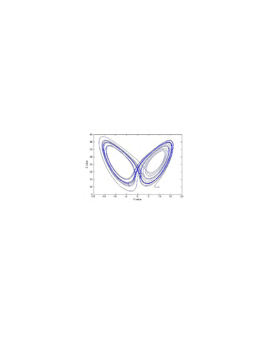
Observe the trajectory of a particle, projected onto the X-Z-plane as shown in Figure 1.
(It should be noted that the intersections in the path are merely a result of the projection
and do not actually occur in three dimensions.) It displays turbulent behavior. The
precise definition of turbulence varies depending on the context and purpose of the
analysis, but one common turbulent characteristic is that the path depicted does not
approach a periodic limit or an equilibrium point. In the center of each of the two loops
is an unstable equilibrium point, and the particle orbits one, then the other, jumping back
and forth in a manner that appears random, though is actually deterministic. Furthermore,
the general form of this trajectory is not dependent upon initial conditions or integration
method. Here the parameter values are b = 8/3, σ = 10, and r = 28, and the initial point is
(10, 0, 10). If this system is perturbed slightly, though the details will change, the general
form will remain.

Historically, closed physical systems were generally believed to approach periodic

behavior. Nonperiodicity was an idea that was slow to come into acceptance. Lorenz
acknowledges and thanks Saltzman for first pointing out the nonperiodic behavior of the
convection equations (Lorenz 141).

2.2 Sensitive to Initial Conditions

One feature of the Lorenz System that had previously been largely ignored from analysis
of physical systems is the fact that even a slight perturbation can alter the outcome
drastically. This characteristic is also sometimes used in definitions of turbulence. The
general line of thinking had previously been that a small difference in initial conditions
would yield a small difference in results, except near unstable equilibria. As it turns out,
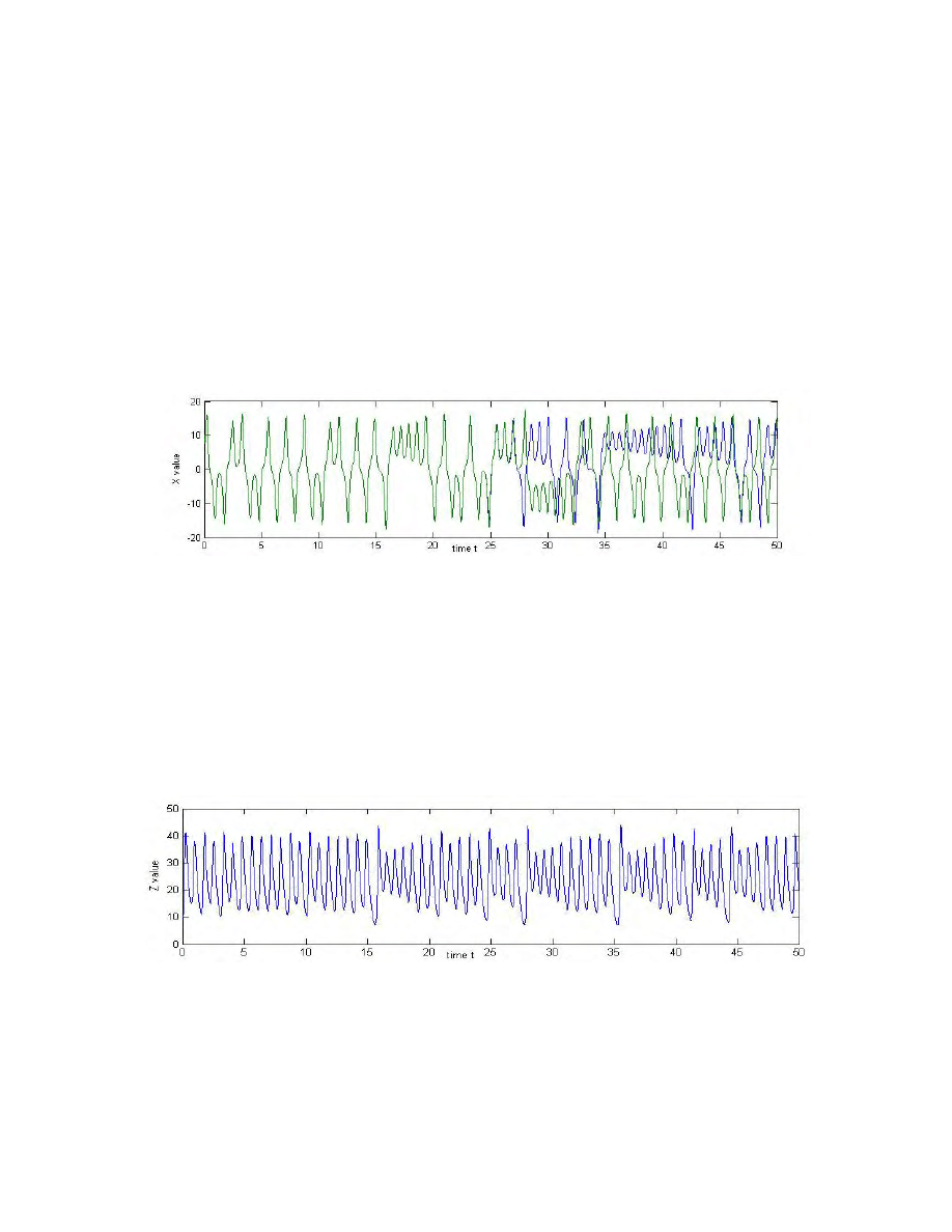
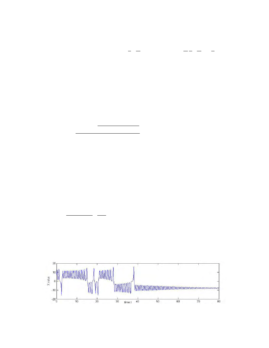
this is not true for most real-world systems. Figure 2 illustrates this phenomenon in the
Lorenz System. Two trajectories begin with very close initial conditions; in particular, X

1

= X

2

= 10, Y

1

= Y

2

= 0, Z

1

= 10, Z

2

= 10.00000000001. For the first 25 time units, the two

trajectories seem identical. However, beyond 30 time units, they seem completely

Figure 1 A numerical solution of the Lorenz equations
projected onto the X-Z plane showing nonperiodic behavior.

unrelated to each other.

It is this property of physical systems that makes long term prediction impossible,

and ultimately dashes the hopes idealistic classical physicists. Strangely, this
unpredictability comes from a completely deterministic system. Although Lorenz
illustrated this phenomenon of sensitivity to initial conditions in a very simple and
elegant manner in his paper, he was not the first to discover it. Poincaré once wrote,
"[S]mall differences in the initial conditions produce very great ones in the final
phenomena. A small error in the former will produce an enormous error in the latter.
Prediction becomes impossible, and we have the fortuitous phenomenon" (Davies 53).
Yet for a long time, people were reluctant to accept these ideas in favor of the non-
chaotic, predictable universe.

2.3 Lorenz's Deterministic Nonperiodic Sequence

The following example comes from Lorenz's paper. It is used to illustrate some of the
implications of the nonperiodic behavior of the sequence of Z-maxima. Lorenz wondered
whether one Z-maximum could be used to predict the next.

It appears that once the Z value crosses a certain threshold, the particle will jump into an
orbit around the other equilibrium, and Z will become suddenly small again. Again, the Z
value will increase until it reaches a certain threshold, then jump back to the original
orbit, and so on (Figure 3). He composed the following figure which plots M

n

against

M

n

1

. That is, given one Z-maximum on the horizontal axis, the vertical axis shows

Figure 2 Two numerical solutions of the Lorenz equations showing sensitivity to initial conditions. The X
values, plotted with respect to time, of two trajectories whose initial positions differ by one one-hundred-
billionth in the Z direction. These two trajectories seem identical until around t = 27.5, at which point they
completely separate forever.

Figure 3 The Z value plotted against time to show the behavior of the sequence of Z-maxima.

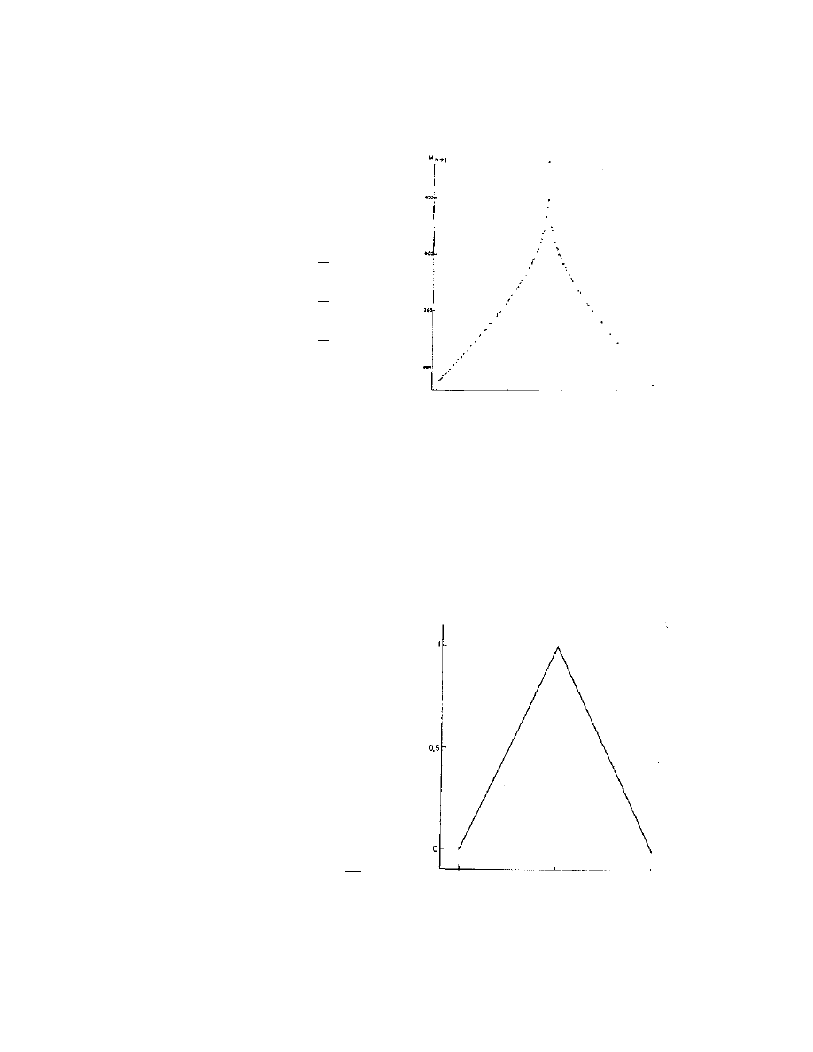
the value of the next Z-maximum (Figure 4). The cusp corresponds to an orbit going to
the origin, located on the local stable manifold.

Lorenz revealed the implications of

this sequence using the following simplified
example.

Consider the sequence

M

0,

M

1,

... of numbers between 0 and 1,

defined as follows.

M

n

1

=2 M

n

if M

n



1
2

M

n

1

is undefined if M

n

=

1
2

M

n

1

=2−2 M

n

if M

n



1
2

Thus, Lorenz's diagram is simplified to
Figure 5. Given an initial M

0

, the

general form of M

n

is given explicitly by

(*)

M

n

=m

n

±2

n

M

0

,

where m

n

is an even integer. This can be shown inductively. Clearly m

0

=0 , and

M

0

is of the desired form. Suppose the statement holds for n

=k . There are two

possibilities for the next iteration,

M

k

1

=2 M

k

=2 m

k

±22

n

M

0

and

M

k

1

=2−2 M

k

=2−2 m

k

∓22

k

M

0

, both of which are of the desired form.

Now consider these cases.

Case 1: M

0

=u/2

p

where u is odd. Then

by (*) and the fact that the sequence remains
between 0 and 1, M

p

−1

=1/2 . Such

sequences represent no convection at all, but
there are only countably many of them.

Case 2:

M

0

=u/2

p

v



where u and v

are relatively prime and odd. If k

0 then

M

p

1k

=u

k

/v where u

k

is even and

relatively prime to v . The number of

possibilities for fractions 0



u

k

v

1 is

finite, so the sequence is periodic. Again,
there are countably many such sequences.

Figure 4 From Lorenz's paper: Corresponding
values of relative maximum of and subsequent
relative maximum of Z for the first 6000 iterations.

Figure 5 From Lorenz's paper: An idealization of
Figure 4 using the M-sequence defined.

Case 3: M

0

is irrational. By (*) we have that for periodic sequences, M

0

−M

k

must be rational (since M

k

=

m

k

1

∓2

k

is rational). The sequence is thus not periodic, but

it still could be quasi-periodic, approaching a periodic sequence asymptotically. To
eliminate this possibility, Lorenz showed that all sequences are unstable to slight
perturbations. Consider two sequences, M

0,

M

1,

... and M

0

' , M

1

' ,... where

M

0

'

=M

0

 for a small  . Then for k0 we have

M

k

'

=M

k

±2

k



, and the

sequence is unstable. Therefore there are uncountably many nonperiodic sequences,
corresponding to the irrational numbers between 0 and 1.

It is interesting to note that in this example, the existence of chaotic behavior

corresponds directly to the existence of irrational numbers, a fact that people were once
even more reluctant to accept. According to legend, when Hippasus first proved the
existence of irrational numbers, he was thrown by the other Pythagoreans from a boat into
the middle of the ocean

[3].

3 Properties and Bifurcations

There exist far too many interesting features of the Lorenz System to discuss in a single
paper. Henceforth the scope of this paper will be limited to some of the behavior of the
system near the equilibria as r increases from an infinitesimal value toward infinity, for
fixed values of the other parameters. To read about the system's other features, a good
place to start is Sparrow's book (see references).

3.1 Dissipative

A system is dissipative if every orbit eventually moves away from infinity. That is,

∃ B⊂ℝ

2

bounded, such that

∀ x

0

∈ℝ

2

,

∃t

0

(depending on x

0

, B ) with the

solution t , x

0

 satisfying t , x

0

∈B ∀ t≥t

0

(Hale & Koçak 394). It can be

shown that the Lorenz System is dissipative by using the Liapunov function

V

=rX

2

 Y

2

 Z−2 r

2

(Sparrow 196).

Then

˙V =2rX ˙X 2 Y ˙Y 2Z−2 r ˙Z

= −2 r X

2

Y

2

bZ

2

−2brZ  .

Choose the bounded region D such that X

∈D⇔ ˙V  X ≥0 , and let c be the maximum

of V in D. Let E be the ellipsoid defined by V

≤c for small 0 . Then

X

∉E ⇒ X ∉D

⇒ ˙V  X ≤− for some 0 ,

and the points on the trajectories passing through

X will be associated with a

decreasing V. Thus the trajectories will eventually enter and remain in E.

It follows from the fact that the divergence of the system is negative, -(σ + b + 1),

that the volume of this region will decrease with e

−b1t

, so the set toward which all

trajectories tend has zero volume (Sparrow 198).

3.2 Symmetric

The Lorenz System is invariant under the symmetry

 X ,Y , Z −X ,−Y , Z  :

− ˙X = −−X −Y 

⇒ ˙X = −X Y 

− ˙Y =r −X −−Y −−X  Z

⇒ ˙Y =rX −Y − XZ

˙Z =−bZ −X −Y =−bZXY .

The invariance of the Z-axis implies that all trajectories on the Z-axis remain on the Z-
axis and approach the origin. Furthermore, since

X

=0,Y 0⇒ ˙X 0

and

X

=0,Y 0⇒ ˙X 0

,

all trajectories that rotate around the Z-axis must move clockwise with increasing time.

3.3 Equilibria

Let us now find the equilibrium points of the system. Solving

 −X Y =0

r X

−Y − X Z =0

−b Z X Y =0

yields

X

=0 , or ±



b

r−1 .

Depending upon the parameter values, we might have as equilibria

0,0,0

,

C

1

=−



b

r−1 ,−



b

r−1 , r−1 , and

C

2

=



b

r−1 ,



b

r−1 , r−1 ,

though the origin is always an equilibrium point.

The behavior of the Lorenz System is quite complex. To examine some simple

bifurcations, first consider the case where two of the parameters are fixed at b = 8/3 and σ
= 10, and let 0 < r < 1. Then the above root has an imaginary part, and the only real
equilibrium is

X

=Y =Z =0 .

In fact, this equilibrium point is a global attractor for 0 < r < 1. To see this, consider the
Liapunov function,

V

= X

2

 Y

2

 Z

2

.

Then,

˙V =2 X ˙X 2 Y ˙Y 2 Z ˙Z

= 2 [1r XY − X

2

−Y

2

−bZ

2

]

⇒ ˙V 0 ∀ X ,Y , Z

.

This last inequality is seen by observing that

1r XY − X

2

−Y

2

0 , i.e. r

X

2

Y

2

XY

−1 ,

since if X ≥ Y (similar for the opposite inequality) then

X
Y

−1≥0 , and 1−

Y
X

≥0 ,so their product,

X
Y

−2

Y
X

≥0

⇒

X

Y



Y

X

−1=

X

2

Y

2

XY

−1≥1r .

Thus beginning at any point away from the origin, the associated value of V must
decrease, and the trajectory will approach the origin.

3.4 The First Bifurcations and "Preturbulence"

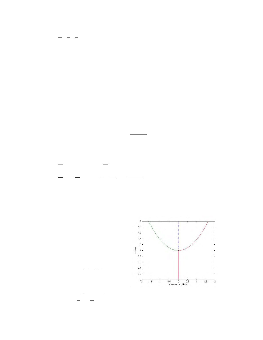
At r = 1 there is a bifurcation, and the other
two equilibria appear. By the symmetry
previously shown, we see that this is a
pitchfork bifurcation. The origin becomes
unstable, and two stable equilibria emerge,

C

1,

C

2

, as seen in the bifurcation

diagram in Figure 6.

Linearizing the system near an

equilibrium point

 X ,Y , Z  using the

Jacobian matrix gives

[

˙X

˙Y

˙Z

]

=

[

−



0

r

−Z −1 −X

Y

X

−b

]

[

X

Y

Z

]

,

Figure 6 Bifurcation diagram varying r from 0 to 2
and fixing the other parameters, showing the X value
of the equilibria.

and setting the determinant minus λI equal to zero gives the eigenvalues as solutions of



3

b1

2

bb−r  Z  X

2

b 1−r  X Y  X

2

b Z =0 .

If the equilibrium point is taken to be the origin, this simplifies to



3

b1

2

bb−r b 1−r=0 .

Since -b is clearly a solution, we factor to get

b

2

1 1−r=0 ,

and the three eigenvalues are:



1

,



2

=

−−1±



1

2

4 r−1

2



3

=−b ,

expressed in such a way to make it clear that



1

0 , 

2

,



3

0 for r > 1. Thus the

origin becomes unstable (Hale & Koçak, Theorem 9.3). This is generally called a saddle,
with a one-dimensional, unstable manifold.

The eigenvalues of a linearization near C

1

and C

2

simplify to be the solutions of



3



2

b1br2 br−1=0 .

If we let b = 8/3 and σ = 10, then all three roots will have negative real part if

r



 b3

−b−1

=

470

19

≡r

H

(Sparrow 10).

Thus if r < r

H

then C

1

and C

2

are stable. For r > r

H

, the two complex eigenvalues have

positive real part, and the equilibria become unstable (Hale & Koçak, Theorem 9.3). At
r = r

H

there is a subcritical Hopf bifurcation. So for values of r above this critical value,

there are three unstable equilibria, yet it has already been shown that no trajectories

Figure 7 A "preturbulent" trajectory at r = 22.7, just before the bifurcation into chaotic behavior.

approach infinity but rather eventually enter a region around the origin. This is where we
begin to see the chaotic behavior similar to that originally seen in Figure 1.

How does the system transition from nonchaotic to chaotic? To see intuitively

what happens to the trajectories as r approaches this critical value, let us look at r = 22.7,
just before the bifurcation (Figure 7). C

1

and C

2

are still stable, so the trajectory

eventually spirals in toward one of them, but before it comes sufficiently close to an
equilibrium, it exhibits "preturbulent" or “chaotic transcient” behavior.

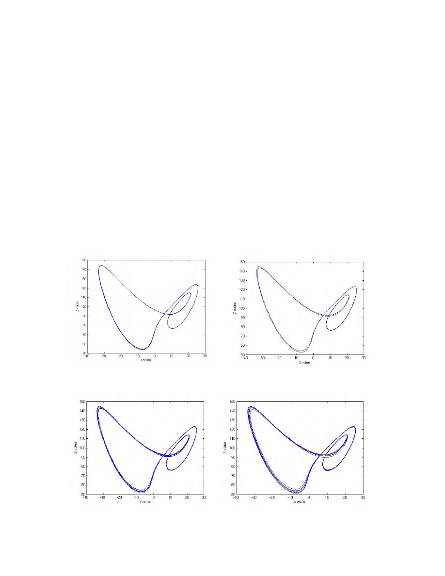
3.5 Period Doubling Windows

For the values 99.524 < r < 100.795 there exists what is called a "period doubling
window." The first period doubling, listed in increasing order of period, occurs at r ≈
99.98. Just above this bifurcation value, trajectories approach a stable periodic orbit that
circles the first equilibrium once, then the second equilibrium twice, which we will
denote [1-2-2], as seen in Figure 8. As r decreases, the period doubles to [1-2-2-1-2-2]
for 99.629 < r < 99.98 (Figure 9). As r continues to approach the lower boundary of this
window, 99.524, there is a cascade of period doubling similar to the behavior of chaotic
one-dimensional maps. For 99.547 < r < 99.629 there is a period of [1-2-2]

4

, for 99.529 <

r < 99.547 there is a period of [1-2-2]

8

, and so on (Figures 10 and 11 respectively).

Figure 8 Stable periodic orbit for r = 100.5.

Figure 9 Stable periodic orbit after the first period
doubling, for r = 99.7.

Figure 10 Stable periodic orbit after the second
period doubling, for r = 99.6.

Figure 11 Stable periodic orbit after the third period
doubling, for r = 99.537.

Not much is known of the particular behavior for values of r just less than the

accumulation point of such cascades, where chaos begins. In general, the period doubling
cascades have the same properties as in scalar maps, such as the Feigenbaum number,

=lim

n

∞

r

n

1

−r

n

r

n

2

−r

n

1

=4.669... which can be used to find the accumulation value r

∞

.

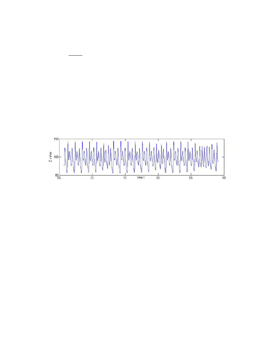
The behavior in the upper half of the period doubling window is interesting as

well. The fact that the window has an upper bound suggests that the system demonstrates
nonperiodic behavior once again as r exceeds it. This is true, and the transition can be
seen through what is called "intermittent chaos." This phenomenon is shown in Figure 12
for r = 100.93. As time progresses, the trajectory tends toward the periodic orbit, but
every so often it lapses into nonperiodic, chaotic behavior for an interval of time. If r is
within the period doubling window, the intermittent chaos will eventually cease, leaving a
periodic orbit, but once r is beyond the upper bound, r

c

, intermittent chaos will occur after

any given time t'. As r moves further from the window, the periods of intermittent chaos
will increase in length until they dominate the trajectory. In fact, the mean length of the
periodic intervals seems to vary at a rate proportional to

r−r

c



−1/2

(Sparrow 63)

[4]

.

There exist two other period doubling windows as r increases. The first is 145 < r

< 166. For 154.4 < r < 166.07 there is a stable symmetric (i.e. with the same symmetry as
shown for the system itself) periodic orbit with a period described by [1-1-2-2]. At r ≈
154.4 the stable symmetric orbit splits into two stable asymmetric periodic orbits with
periods described by [1-1-2-2], producing between them an unstable periodic orbit.
These orbits undergo simultaneous period doubling bifurcations as r decreases in a
manner similar to that of the first window (Sparrow 59).

The final period doubling window is for 214.364 < r, with period described by a

symmetric stable [1-2] orbit. This window is similar to the previous, except that for r >
313, the lowest period orbit continues to exist. There is no intermittent chaos as r
increases. In fact, for large enough r, it is believed that this stable periodic orbit unioned
with the three equilibria compose all of the non-wandering set, though this simple
behavior depends on our particular choice of b and σ (for a theoretical justification of this
claim, see Sparrow, chapter 7)

[5]

.

4 Afterword

Lorenz's paper has spawned many deep and detailed analyses of this system. For a fairly
rigorous discussion of other features of the system, such as homoclinic explosions,
manifolds, another derivation, etc., see Sparrow's book. For an entertaining, qualitative
dramatization of chaos and its implications, see Gleick's book. Lorenz's article itself is an

Figure 12 Intermittent chaos just above the period doubling window, for r = 100.93.

invaluable milestone in physics and mathematics, and is highly recommended. Although
it was published in the Journal of Atmospheric Sciences, it is essentially a mathematics
article and is elegant in its simplicity.

Many higher dimensional systems have been designed as extensions of the Lorenz

System. In fact, the system itself is a simplification of fluid convection, and higher order
systems of fluid convection have been studied. Extensions of the Lorenz System have
similar symmetries and demonstrate similar behavior, though more complex. In one such
example, there are two equilibrium tori that act like the equilibria in the Lorenz System,
with trajectories orbiting one torus, then the other, in a nonperiodic manner. Examination
of these systems generally involve analyzing the way the system changes with a changing
parameter, r, just as in the Lorenz System.

The conclusion of Lorenz's paper relates his theory to the atmosphere. Bounded

finite dimensional systems must eventually come arbitrarily close to any previous state.
We could then expect an analogue in the weather—i.e. a point in time when the
atmosphere seems to be in a state identical to to a previously observed state. If the system
is nonchaotic, then the weather will remain arbitrarily close to its past behavior, and
weather forecasting will be a breeze. On the other hand, if an analogue occurs followed
by new weather patterns, no forecasting scheme could be correct both times, and the
system is unpredictable.

By now it is generally accepted that real physical systems contain this inherent

unpredictable quality. Sensitivity to initial conditions, sometimes dubbed the "butterfly
effect," is commonly described using an old folk poem in which a misplaced nail causes a
kingdom to fall (see Gleick 23). Instead of repeating this example, I'd like to close with a
Steinbeck passage that describes a real-life example of sensitivity to initial conditions that
is, perhaps, a more accurate analogy.

"Two gallons is a great deal of wine, even for two
paisanos. Spiritually the jugs may be graduated thus: Just
below the shoulder of the first bottle, serious and
concentrated conversation. Two inches farther down,
sweetly sad memory. Three inches more, thoughts of old
and satisfactory loves. An inch, thoughts of old and bitter
loves. Bottom of the first jug, general and undirected
sadness. Shoulder of the second jug, black, unholy
despondency. Two fingers down, a song of death or
longing. A thumb, every other song each one knows. The
graduation stops here, for the trail splits and there is no
certainty. From this point on anything can happen
(Steinbeck 43-4)."

REFERENCES

DAVIES, Paul. "The Cosmic Blueprint." Orion Productions, 1988. Simon and Schuster, New York.
GLEICK, James. "Chaos: Making a New Science." James Gleick, 1987. Penguin Books, New York.
HALE, J. and H. Koçak. "Dynamics and Bifurcations." Springer-Verlag New York Inc., 1991. New York.
KUNDU, Pijush K. and Ira M. Cohen. "Fluid Mechanics: Second Edition." Academic Press, 2002.
LORENZ, Edward N. "Deterministic Nonperiodic Flow." Journal of the Atmospheric Sciences, 20, 130-
141, 1963.
SALTZMAN, B. "Finite amplitude free convection as an initial value problem—I ." Journal of the
Atmospheric Sciences, 19, 329-341, 1962.
SPARROW, Colin. "The Lorenz Equations: Bifurcations, Chaos, and Strange Attractors." Springer-Verlag
New York Inc., 1982. New York.
STEINBECK, John. "Tortilla Flat." John Steinbeck, 1935. Random House, New York.

All figures not cited were generated by the author using MATLAB 6.5.

COMMENTS BY PROFESSOR ANDY FOSTER

[1] 'In fact, experimentalists would routinely hide (i.e. not publish) data from real systems exhibiting these
types of behavior.'

[2] 'As we have seen, this is usually no problem, because of topological equivalence, etc. But ... the
prevalent mindset is still that systems are classically predictable.'

[3] 'This “tent map” construction from the original flow is interesting, isn't it? Notice that the tent map is

ℝ

1

, so it is simpler than the Poincaré map, which would be

ℝ

2

.'

[4] 'For intermittent chaos, see Y. Pomeau and P. Manneville, Comm. Math. Phys. 74, 189-197 (1980).'

[5] '...Did you know that the Lorenz system is not structurally stable? Yes, it has dense sets with and
without saddle-saddle connections which can switch back and forth under arbitrarily small perturbations.
So, what appears to be a stable chaotic set is not stable!'