

2012 WILEY-VCH Verlag GmbH & Co. KGaA, Weinheim

www.plant-soil.com

J. Plant Nutr. Soil Sci. 2012, 000, 1–8

DOI: 10.1002/jpln.201100361

1

Analysis of soil fertility and its anomalies using an objective model

Francisco J. Moral

1

*, Francisco J. Rebollo

2

, and José M. Terrón

3

1

Departamento de Expresión Gráfica, Escuela de Ingenierías Industriales, Universidad de Extremadura. Avda. de Elvas, s/n. 06071 Badajoz,
Spain.

2

Departamento de Expresión Gráfica, Escuela de Ingenierías Agrarias, Universidad de Extremadura. Carretera de Cáceres s/n,
06007 Badajoz, Spain.

3

Departamento de Cultivos Extensivos, Centro de Investigación La Orden-Valdesequera, Consejería de Empleo, Empresa e Innovación,
Junta de Extremadura. 06187 Guadajira, Badajoz, Spain.

Abstract

In this work, the use of an objective method, the formulation of the Rasch measurement model,
which synthesizes data with different units into a uniform analytical framework, is considered to
get representative measures of soil fertility potential in an experimental field. Thus, two types of
information about the soil were obtained from soil samples taken at 70 locations: first, the tex-
tural components were determined, and, secondly, deep (ECa-90) and shallow (ECa-30) soil
apparent electrical conductivity, approximately 0–90 and 0–30 cm depths, respectively, were
measured. A latent variable, denominated soil fertility potential, was defined. It is supposed, and
later it is verified, that all soil properties previously indicated have a marked influence on the
latent variable. The adequate assignment of categorical values across properties measures and
the good fit of the data are checked as a previous phase to properly compute the Rasch meas-
ures. After applying the Rasch methodology, it was obtained that both electrical conductivities
are the most influential properties on soil fertility potential, getting moreover a ranking of all soil
samples according to their fertility potential and the unexpected behaviors, called misfits, of
some soil samples, which constitute a very useful information to better match soil and crop
requirements as they vary in the field, being a rational basis for a site-specific crop manage-
ment.

Key words: Rasch model / texture / soil apparent electrical conductivity / site-specific soil management

Accepted January 8, 20152

1 Introduction

Obtaining a measure of soil fertility potential, in the sense the
crop-production potential is influenced by soil fertility, is not
easy due to the fact that different variables can influence its
quantification. Soil fertility is affected by many soil physical
and chemical variables, which, in turn, depend on various
local factors, such as climatic conditions.

During the last years, the management of agricultural fields
tends to be differential, defining areas with similar character-
istics, homogeneous zones, which will require different treat-
ments. Variability management can improve the productivity
and profitability of crop production and also to protect envir-
onmental resources. This can be accomplished by spatially
varying fertilizer according to crop requirement. Delineation
of management zones can be done using some rather com-
plex techniques, and their results need a subsequent inter-
pretation which is usually quite subjective (Morari et al.,
2009).

Another problem is the correct choice of the variables that
can better characterize soil fertility. In general, soil texture
properties and apparent electrical conductivity (ECa), the last
integrating the response of several soil physical and chemical
properties, have been utilized to characterize different zones

in agricultural soils and, in consequence, provide indications
about their fertility (Moral et al., 2010).

With the aim of considering and summarizing data from differ-
ent variables, the Rasch model has been used successfully
in some environmental applications (e.g., Moral et al., 2006).
However, despite the useful information it can generate, this
technique had not been used in agronomic or soil research
until the work of Moral et al. (2011), in which different man-
agement zones were delimited in an experimental field taking
into account the formulation of the Rasch model with the aim
of integrating soil textural and ECa data into an overall vari-
able. Thus, an estimation of the soil fertility potential was ob-
tained (the Rasch measure) and it was utilized as previous
information to carry out a geostatistical study and, later, by
means of an equal-size classification method to delineate the
homogeneous zones. However, as it was recognized in the
aforementioned work, besides providing soil-fertility-potential
estimates, the output of the Rasch model contains a lot of
useful information as, for example, if all individual variables
support the latent variable, or if there is any anomaly related
to a particular soil property. This information could be very
important from an agronomic point of view.

* Correspondence: Dr. F. J. Moral; e-mail: [e-mail]

In this work we aim to: (1) analyze the proper use of the
Rasch model; (2) study the misfits since they could be an
important source of information about anomalies in any soil
property or data at every sample location; and (3) incorporate
this information in a geographical information system (GIS) to
visualize where anomalies are located and their possible spa-
tial patterns.

2 Materials and methods

2.1 The Rasch model

The Rasch model is a simple but at the same time very
powerful Item Response Theory model for measurement,
being the most viable proposition for practical testing since it
can be applied in the context in which individual, soil sam-
ples, interacts with items, soil properties (Ren et al., 2008).

If guided by a reasonably coherent conceptual goal, the
Rasch model can synthesize and consolidate seemly dispa-
rate data into a uniform analytical framework. The purpose of
this procedure is to transcend several heterogeneous meas-
ures of soil properties (clay, silt, sand, ECa-30, and ECa-90
data [soil apparent electrical conductivity, approximately at
0–90 and 0–30 cm depths]) and consolidate them into an
overall variable that simplifies interpretation of soil fertility
potential.

One way to form a single synthesis of the items, which are
expressed in different measurement units, is by means of a
common referent that holds them all together. This referent,
which will be adimensional and constitute the latent variable
or construct, shall be termed “soil fertility potential”. To
achieve an adimensional characterization, we first categorize
the data corresponding to the considered individual soil prop-
erties. In particular, five categories or levels are established
for all properties and these categories are the same for each
soil property. A measure assigned to level 0 indicates the low-
est contribution to soil fertility potential and, on the contrary, a
measure assigned to level 9 indicates the highest contribution
to soil fertility potential.

The data are arranged in matrix form, where the rows are the
locations where soil were taken and the columns the soil
properties. Each cell can be represented by X

ij

, where i varies

from 1 to 5 (soil properties) and j from 1 to 70 (sampling loca-
tion), and its value reflects the category. One possible way of
obtaining a ranking is to sum the categories of all the soil
properties for each sampling location, and of all the sampling
location for each soil property, i.e., summing by rows or by
columns. However, these sums establish separate rankings
for the sampling locations and the soil properties, and the
procedure does not discriminate between ranking sampling
locations in terms of soil properties and soil properties in
terms of sampling locations.

The Rasch model uses the traditional total score (the sum of
the item ratings) as a starting point for estimating response
probabilities. The model is based on the simple idea that
some items (in this case study soil properties) are more

important to subjects (in this case soil samples) than other
items. Thus, the Rasch model constructs a line of measure-
ment with the items placed hierarchically on this line accord-
ing to their importance to subjects. The validity of a given test
can be assessed through examination of this item ordering,
i.e., by assessing whether all items work together to measure
a single variable.

Rasch measurement construction applies a stochastic Gutt-
man model to convert rating scale observations into linear
measures, to which linear statistics can be usefully applied,
and tests for goodness-of-fit to validate its item calibrations
and subject measures. In this case study, the Rasch model
combines calibrations of soil-property items additively to soil-
sample measures to define soil-fertility-potential probabilities.
This stochastic conjoint additivity specifies a Guttman scale
of probabilities to which the data are fitted (Rasch, 1980).

In order to determine how well each item contributes to the
soil-fertility-potential measurement, chi-square fit statistics,
known as Infit and Outfit mean-square (Infit and Outfit
MNSQ), ratios of observed residual variance to expected
residual variance, should be computed. Infit is an informa-
tion-weighted or inlier-sensitive fit statistic that focuses on the
overall performance of an item or subject. Outfit is an outlier-
sensitive fit statistic that picks up rare events that have
occurred in an unexpected way. Its expectation is 1. Values
> 2 indicate unexplained randomness throughout the data
(Smith, 1996). Usually, items that fall between the infit and
outfit limits of 0.6 and 1.5 are accepted and those with values
beyond these thresholds have to be removed (Bond and Fox,
2007).

More information about the mathematical formulation of the
Rasch model can be obtained in Moral et al. (2011).

2.2 Data collection and treatment

Soil samples were collected at a farm called Cerro del Amo
(38°58

′

14

″

N, 6°33

′

394 W, 225 m asl, Datum WGS84), 37 km

E of Badajoz (SW Spain). Its area is

≈

33 ha. Seventy geo-

referenced soil samples were taken from the top layer
(0–20 cm), using a stratified random sampling scheme.
A more detailed description of the characteristics of the
experimental field and the soil sampling can be obtained in
Moral et al. (2011).

For each soil sample, the particle-size distribution was deter-
mined by gravitational sedimentation using the Robinson
pipette method (Soil Conservation Service, 1972), after
passing the fine components through a 2 mm sieve, and
ECa-30 and ECa-90 data for all locations were obtained
from kriged maps (after fitting a spherical variogram, with
range = 288.4 m, sill = 0.505, nugget effect = 0.093, to the
experimental one, and using the ordinary kriging algorithm),
previously generated from different transects of the measure-
ments of soil apparent electrical conductivity which were car-
ried out using a direct contact sensor (Moral et al., 2010).

WINSTEPS v. 3.69 computer program was employed to
conduct the formulation of the rating scale Rasch model



2012 WILEY-VCH Verlag GmbH & Co. KGaA, Weinheim

www.plant-soil.com

2

Moral, Rebollo, Terrón

J. Plant Nutr. Soil Sci. 2012, 000, 1–8

(Linacre, 2009). To do that, firstly, a transformation of the soil
properties measures to common categories was performed
and data were arranged in a matrix whose rows are the soil
samples and columns are the soil properties (Tab. 1). For soil
texture properties, according to the characteristics of the
experimental field, the ideal percentage of each texture class
was about a third of the total; in consequence, for an interval

≈

33% of clay, silt, or sand content the maximum categorical

value, 5, was assigned. For ECa-30 and ECa-90, the highest
categorical values correspond to the classes with highest
measures. The other categories were associated with
classes in which their amplitude depends on the maximum
and minimum values of each soil property. The assignment of
categorical values across properties measures are displayed
in Tab. 2.

With 5 soil properties taken into account, the highest possible
raw score for the soil samples is 25 (the most potentially
fertile) and the lowest possible score is 0 (the least potentially
fertile).

As outputs of the program, the empirical hierarchy of soil
properties is illustrated using variable map and related to all
soil samples, with each reported in logits, the statistics show
how well the data fit the model and, additionally, soil sample
and property misfits are explained.

3 Results and discussion

3.1 Data response to the model

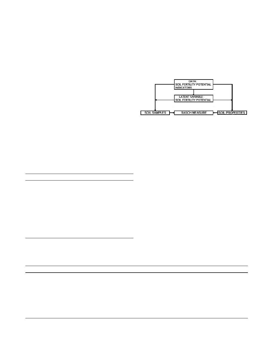
The contribution of the soil properties considered, in this case
study clay, silt, and sand contents, ECa-30 and ECa-90, to
obtain a representative measure of soil fertility potential at
each sampling location was performed with the formulation of
the Rasch model through the stages displayed in Fig. 1.

After processing the matrix of categorical values by the WIN-
STEPS program, the output was several results with table or
diagram format. The first information to be taken into account
is if the data fit the model reasonably. To do this, the Infit and
Outfit statistics have to be analyzed. Thus, according to the
Infit and Outfit MNSQ values contained in Tabs. 3 and 4, 0.96
and 0.97, there is a clear evidence about the agreement be-
tween the data and the model. Moreover, the mean standar-
dized (ZSTD) Infit and Outfit, which are the sum of squares
standardized residuals given as a Z-statistics (Edwards and
Alcock, 2010), are expected to be 0, being in this study –0.2
for samples and for items (Tabs. 3 and 4), denoting that the
data fit the model better than expected.

Another parameter to be considered is the standard deviation
of the Infit MNSQ (Bode and Wright, 1999), which is an index
of the overall misfit for soil samples and properties (a value

<

2 is considered acceptable). There is not important misfits

in this case study because their values are 0.75 and 0.15 for
soil samples and properties, respectively, also indicating an
acceptable overall fit of the data.

With the aim of estimating the internal consistency of soil
samples and properties, in the sense of determining the



2012 WILEY-VCH Verlag GmbH & Co. KGaA, Weinheim

www.plant-soil.com

Table 1: Matrix of categorical values used to perform the formulation
on the Rasch measurement model.

Sample

Clay

Sand

Silt

ECa-30

a

ECa-90

1

4

3

3

4

4

2

3

3

3

3

3

3

4

3

3

5

4

4

4

4

3

5

5

...

...

...

...

...

...

67

3

2

3

2

3

68

3

3

3

3

3

69

3

2

2

4

4

70

2

5

3

5

5

a

ECa-30, soil apparent electrical conductivity, 0–30 cm depth;

ECa-90, soil apparent electrical conductivity, 0–90 cm depth.

Table 2: Soil properties measures recoded into rating scale categories.

Rating scale value

1

2

3

4

5

Clay / %

<

13.8 or > 52.8

(13.8–19.4] or
[47.2–52.8)

(19.4–25.0] or
[41.7–47.2)

(25.0–30.5] or
[36.1–41.7)

(30.5–36.1)

Sand / %

> 70.4

<

6.9 or [59.8–70.4)

(6.9–17.4] or
[49.2–59.8)

(17.4–28.0] or
[38.6–49.2)

(28.0–38.6)

Silt / %

<

7.8 or [58.9–66.1)

(7.8–15.1] or
[51.6–58.9)

(15.1–22.4] or
[44.3–51.6)

(22.4–29.7] or
[37.0–44.3)

(29.7–37.0)

ECa-30

a

/ mS m

–1

(3.46–7.36]

(7.36–11.26]

(11.26–15.16]

(15.16–19.05]

(19.05–22.95]

ECa-90 / mS m

–1

(18.81–29.59]

(29.59–40.37]

(40.37–51.15]

(51.15–61.93]

(61.93–72.71]

a

ECa-30, soil apparent electrical conductivity, 0–30 cm depth; ECa-90, soil apparent electrical conductivity, 0–90 cm depth.

Figure 1: Diagram of the phases involved in the formulation of the
Rasch model.

J. Plant Nutr. Soil Sci. 2012, 000, 1–8

Analysis of soil fertility and its anomalies 3

degree to which measures are free from error and yield con-
sistent results, there is a reliability statistics. A better reliability
is obtained when this statistics is close to 1; acceptable val-
ues would be > 0.7 (Sekaran, 2000). In this study, reliability
was 0.77 and 0.87 for soil samples and properties, respec-
tively; thus, the consistency of data is adequate and probably
measures have not significant errors.

When the assignment scale was checked to verify how it has
been utilized, according to Linacre (2009), there was a strong
evidence to assert it was properly designed, with 5 cate-
gories: the “observed average” and the “structure calibration”
increase by category value, the Infit and Outfit MNSQ values
are between 0.6 and 1.5, and the “observed average” values
are similar to the “sample expected” ones (Tab. 5). There is

no a general rule to initially define the correct number of cate-
gories. Thus, in this case study, a previous analysis was car-
ried out with 10 categories, finding some results which indi-
cate that this number was not adequate, i.e., the “observed
average” and the “structure calibration” did not increase by
category value, and some Infit and Outfit MNSQ values were
out of the recommended range. However, data fit the model
reasonably, since the Infit and Outfit MNSQ values were be-
tween 0.98 and 1, and reliability was 0.80 and 0.87 for soil
samples and properties, respectively. Although the optimum
number of categories was not 10, the study could have
continued (Moral et al., 2011).

As it was previously indicated, with 5 categories the response
scale use is more adequate. This was also checked with an



2012 WILEY-VCH Verlag GmbH & Co. KGaA, Weinheim

www.plant-soil.com

Table 3: Overall model fit information. Summary of all soil samples (70).

Total score

a

Count

Measure

Model error

Infit MNSQ

Infit ZSTD

Outfit MNSQ

Outfit ZSTD

Mean

17.3

5

0.77

0.57

0.96

–0.2

0.97

–0.2

Standard Deviation

3.9

0

1.21

0.06

0.75

1.3

0.76

1.3

Maximum

23.0

5

2.69

0.79

3.33

2.6

3.32

2.6

Minimum

7.0

5

–2.88

0.53

0.11

–2.7

0.11

–2.7

a

Total score, sum of points of the common scale considering all soil properties; count, soil properties taken into account; measure, logit position

of the soil; properties along the straight line that represents the latent variable, soil fertility potential; model error, standard error of
measurement; Infit and Outfit MNSQ, mean-square fit statistics to verify if items fit the model; Infit and Outfit ZSTD, standardized fit statistics to
verify if items fit the model.

Table 4: Overall model fit information. Summary of all soil properties (5).

Total score

a

Count

Measure

Model error Infit MNSQ

Infit ZSTD

Outfit MNSQ Outfit ZSTD

Mean

242.2

70.0

0.00

0.15

0.97

–0.2

0.97

–0.1

S.D.

18.6

0

0.42

0.00

0.15

1.0

0.19

1.2

Max.

262.0

70.0

0.57

0.16

1.23

1.4

1.26

1.6

Min.

217.0

70.0

–0.45

0.15

0.75

–1.6

0.73

–1.8

a

Total score, sum of points of the common scale considering all soil samples; count, soil samples taken into account; measure, logit position of

the soil samples along the straight line that represents the latent variable, soil fertility potential; model error, standard error of measurement; Infit
and Outfit MNSQ, mean-square fit statistics to verify if items fit the model; Infit and Outfit ZSTD, standardized fit statistics to verify if items fit the
model.

Table 5: Response scale use.

Category

Observed
count

a

Observed
average

Sample
expected

Infit
MNSQ

Outfit
MNSQ

Structure
calibration

1

17

–1.25

–1.73

1.47

1.39

None

2

51

–0.26

–0.42

1.20

1.24

–2.13

3

115

0.29

0.51

0.78

0.71

–0.75

4

88

1.19

1.29

1.33

1.32

1.18

5

79

2.08

1.86

0.66

0.70

1.70

a

Observed count, number of times the category was selected considering all samples and soil properties; observed average, mean value of

logit positions modeled in the category; sample expected, optimum values of the average logit positions for the data; Infit and Outfit MNSQ,
mean-square fit statistics to verify if items fit the model; structure calibration, logit calibrated difficulty of the step representing the transition
points between one category and the next.

4

Moral, Rebollo, Terrón

J. Plant Nutr. Soil Sci. 2012, 000, 1–8

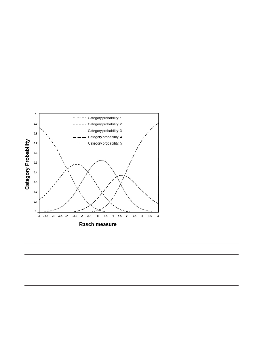
additional tool, the probability curves, which represent the
likelihood of category selection against the Rasch measure.
In Fig. 2, it can be seen that each category value is the most
likely at some point on the continuum, i.e., all categories have
been used, and there is not category inversions, i.e., a higher
category is more likely at a higher point than a lower category
(for instance, if the Rasch measure is –1.5, the most likely
category assignment is 2, and if the Rasch measure is 1, the
most likely category assignment is 3). Consequently, all cate-
gories have been utilized and are behaving according to
expectation.

The final step consists in examining if each soil property fits
the general pattern of the model and contributes to support
the underlying latent variable, soil fertility potential. According
to Bode and Wright (1999), acceptable fit of each item
implies that the Infit and Outfit MNSQ should be between

0.6 and 1.5, and the Infit and Outfit ZSTD between –3 and 2.
In this case study, all these values are in the proposed inter-
vals (Tab. 6), indicating that all considered soil properties
have an important influence and support the soil fertility
potential.

3.2 Analysis of the Rasch measure: soil fertility

potential

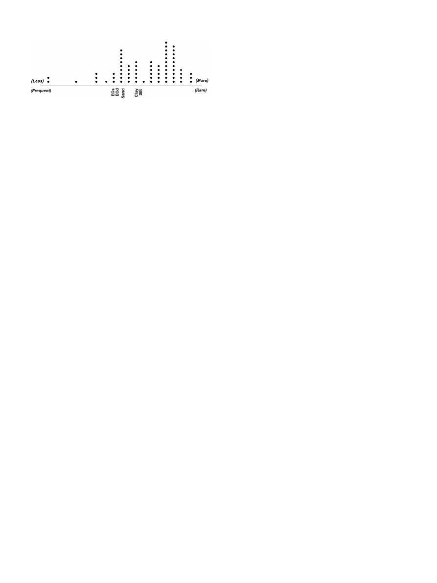
As an output of the Rasch model, all soil samples and their
properties are displayed in the same scale (Fig. 3). Thus, the
relative distribution of the soil samples is provided in the
upper half of the continuum, according to the associated ferti-
lity potential, which has been achieved by means of the five
soil properties taken into account (clay, silt, sand, ECa-30,
and ECa-90), and, similarly, the soil properties are provided



2012 WILEY-VCH Verlag GmbH & Co. KGaA, Weinheim

www.plant-soil.com

Figure

2:

Probability

curves

for

the

five

categories considered in the case study.

Table 6: Item fit statistics. Influence of each soil property on the fertility potential in the experimental field (5 soil properties are considered).

Item

Total
Score

a

Measure

Infit
MNSQ

Infit
ZSTD

Outfit
MNSQ

Outfit
ZSTD

Silt

217

0.57

1.02

0.6

1.09

0.6

Clay

223

0.43

1.23

1.4

1.26

1.6

Sand

251

–0.19

0.75

–1.6

0.73

–1.8

ECd

258

–0.36

0.91

–0.5

0.87

–0.70

ECs

262

–0.45

0.93

–0.4

0.90

–0.70

Mean

242.2

0.00

0.97

–0.2

0.97

–0.2

S.D.

18.6

0.42

0.15

1.0

0.19

1.2

a

Total score, sum of points of the common scale for each soil property considering all samples (70); measure, position of each soil property

along the straight line that represents the latent variable, soil fertility potential; Infit and Outfit MNSQ, mean-square fit statistics to verify if items
fit the model; Infit and Outfit ZSTD, standardized fit statistics to verify if items fit the model.

J. Plant Nutr. Soil Sci. 2012, 000, 1–8

Analysis of soil fertility and its anomalies 5

in the lower half of the diagram, classified according to the
fertility-potential measure of the soil samples.

The soil property that obtained the highest measure, and is to
the right in the continuum (Fig. 3), is the silt content (measure =
0.57; see Tab. 6). This means it is the less common soil property.
It can be seen in Tab. 6 that silt soil content is the property that
exerts the lowest influence on soil fertility; its raw score was the
lowest. At the other extreme, to the left, both ECa-30 and
ECa-90 are situated (measure = –0.45 and –0.36, respectively;
see Tab. 6). They are the more common soil properties because
most soil samples reach an optimum level of them. According to
Tab. 6, ECa-30 and ECa-90 have the highest raw score and
the lowest measure. Almost all soil samples are influenced by
ECa-30 and ECa-90, both being the most influential proper-
ties on the soil fertility in the experimental field.

Analysis of Fig. 3 displays a continuous distribution of soil
samples, with most of them aggregated. However, some of
them, located to the left in the continuum, have very low
score, denoting their low fertility potential. But, as it was pre-
viously indicated, a majority of soil samples, located to the
right, has adequate properties or propensity for inducing soil
fertility. A ranking of all soil samples according to their soil fer-
tility potential, their Rasch measure, can be obtained, indicat-
ing where the most suitable places for crops are located,
while, on the contrary, those which got lower measure, being
potentially less fertile, are also determined. In this case study,
no sample reached the maximum score of 25 points,
although three samples reached 23 points and some of them
have more than 20 points, obtaining in consequence a high
Rasch measure and denoting good conditions to be poten-
tially very fertile; the minimum score was only 7 points.

Another ranking of all considered soil properties have been
obtained as an output of the Rasch model. According to the
order established after processing all data, silt soil content is
the property with higher measure, followed by clay content,
later, sand content and, finally, ECa-30 and ECa-90. Thus,
the influence of each soil property on soil fertility potential in
the experimental field has been obtained. Soil properties with
lower measure, ECa-30 and ECa-90, have the greatest influ-
ence on soil fertility potential; in contrast, the one with higher

measure, silt content, is the soil property that less influence
exerts on soil fertility potential. This is in accordance with
some previous works (Moral et al., 2010, 2011).

Therefore, the establishment of a ranking according to prop-
erties of the soil samples should be fundamental in establish-
ing a crop in a field, since the most suitable conditions of soil
fertility can be expected in areas where soil samples have
achieved higher measure.

3.3 Misfit analysis: anomalies in soil fertility

potential

Results obtained after applying the Rasch model allow us to
detect the soil samples which do not follow the general pattern
(misfits). From a quantitative point of view, it can be found those
that do not endorse the model, or do not reach expected levels,
because the measure is low (negative residuals) or high
(positive residuals). Misfits can be analyzed from the soil-
properties point of view, determining the soil samples which
show distortions in any property with respect the general cri-
teria of all other samples, or from the soil-samples perspec-
tive, analyzing in which soil property misfit occurred.

Taking into account the soil properties, positive misfits are
found in those soil samples with higher fertility potential than
it can be expected, according to the overall measure of all
processed data. Negative misfits correspond to the soil sam-
ples that attain a lower level of fertility potential than it is
expected for their position in the ranking. In this study, misfit-
ting samples were only found for one soil property: clay con-
tent. Two misfitted soil samples had a negative sign (Tab. 7).
This is due to the fact that they are samples that even though
they have obtained a high score in the ranking, they do not
contain an adequate clay percentage, i.e., it was expected
they would have had a more adequate clay content, concre-
tely their score should be 3. Moreover, these misfitted soil
samples have the highest scores in ECa-30 and ECa-90 and
vice versa, which was not expected. The two samples with
positive misfits obtained a very low score in the ranking, but
they had an adequate percentage of clay, which was not
expected. It is curious to denote that these soil samples,
unlike the previous ones, have a very low score in ECa-30
and ECa-90, so they do not follow the expected pattern, that
is, higher clay content would have led to higher ECa-30 and
ECa-90. In fact, the score for both samples is two units lower
than it is expected. The remaining 66 soil samples follow the
expected pattern, i.e., higher clay content leads to higher
ECa-30 and ECa-90, usual in these soils (Moral et al, 2010).

From the soil-samples perspective, eight samples displayed
misfit at least in one soil property (Tab. 8). Sample 56 was the
worst case, showing three misfits, for clay content, ECa-30,
and ECa-90. The clay content has a positive residual where-
as the ECa-30 and ECa-90 have negative residuals, so it cor-
responds to a location that does not follow the expected pat-
tern previously indicated, i.e., higher clay content corre-
sponds with higher ECa-30 and ECa-90. Samples 5 and 51
have a very low score in clay content, but in ECa-30 and
ECa-90 the score is high, so they display a negative residual



2012 WILEY-VCH Verlag GmbH & Co. KGaA, Weinheim

www.plant-soil.com

Figure 3: Soil samples and properties in the same scale. The straight
line represents the latent variable: soil fertility potential. Distribution of
soil samples (points) is above the line: to the right those more
potentially fertile; to the left those less potentially fertile. Soil
properties are below the line: to the right less common (rare)
properties, with lower influence on soil fertility; to the left more
common (frequent) properties, with higher influence on soil fertility.
ECd and ECs are deep (ECa-90) and shallow (ECa-30) soil apparent
electrical conductivity, approximately 0–90 and 0–30 cm depths,
respectively.

6

Moral, Rebollo, Terrón

J. Plant Nutr. Soil Sci. 2012, 000, 1–8

in clay content because their values are not according to the
model. However, on the contrary, sample 33 has a positive
misfit in clay content because a lower value was expected
due to its low ECa-30 and ECa-90.

Another group of misfits is related to the silt content. Two
samples, 48 and 57, have positive residuals in silt content;
they do not follow the expected pattern that higher silt content

would have led to higher ECa-30 and ECa-90 (Moral et al.,
2010), similar to the relationship between clay content and
ECa-30 and ECa-90. Just the opposite, sample 13 has a neg-
ative residual in silt content because its score is too low for its
ECa-30 and ECa-90 levels. The last misfit is related to the
sand content in sample 26. It is higher than expected, prob-
ably due to the particular condition at this location. In this
case study, only 8 of 70 samples,

≈

10%, show some misfit,

denoting how the overall fit of the data to the model is quite
good, as it was initially checked.

The misfit analysis is an important tool to find the locations
where an anomaly exists and is also useful to find the main
deficiencies of any soil property which could more notably
affect soil fertility potential. When this information is introduced
in a GIS, we can visualize the locations where misfits are appar-
ent and analyze their patterns, if they exist. Moreover, com-
parisons between different soil samples, and consequently
between different locations, and also site-specific amend-
ments of any soil property with inadequate levels can be car-
ried out, which could lead to higher soil fertility potential.

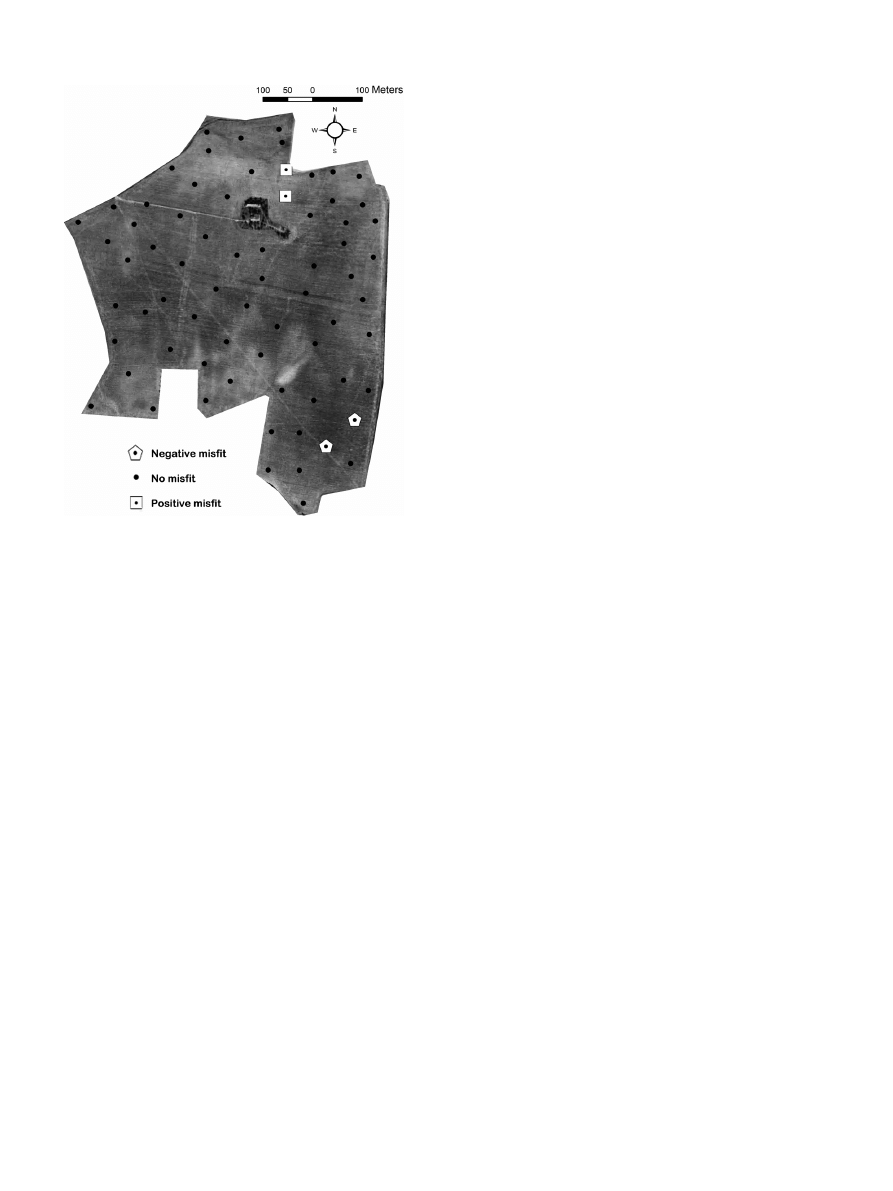
In Fig. 4, locations where soil-clay-content misfits exist are
shown; the two positive and negative misfits are both located
together, denoting there is an excess of this textural property
in one zone of the field and a shortage of the same property
in the other zone, with respect to the optimum level to reach a
higher soil fertility potential. If it is necessary, any work to
amend this soil property should be conducted in these zones.

4 Conclusions

The successful formulation of the Rasch model with the aim
of estimating soil fertility potential is the novel aspect of this
work. It has been determined that the data reasonably fit the
model and all considered soil properties (particle-size distri-



2012 WILEY-VCH Verlag GmbH & Co. KGaA, Weinheim

www.plant-soil.com

Table 7: Misfits for clay content. The score indicates the points for each soil sample considering only this soil property, clay content. Positive
and negative misfits are indicated by the sign.

Soil sample

1

2

3

4

5

6

7

8

9

10

11

12

13

14

15

Score

4

3

4

4

1

2

4

2

3

4

2

3

4

4

4

Misfit

–2

Soil sample

16

17

18

19

20

21

22

23

24

25

26

27

28

29

30

Score

3

3

2

3

4

4

4

4

3

4

2

5

3

4

4

Misfit

Soil sample

31

32

33

34

35

36

37

38

39

40

41

42

43

44

45

Score

2

4

3

3

3

3

4

3

4

3

4

4

3

3

4

Misfit

2

Soil sample

46

47

48

49

50

51

52

53

54

55

56

57

58

59

60

Score

3

2

2

4

3

1

3

2

3

3

4

3

3

3

3

Misfit

–2

2

Soil sample

61

62

63

64

65

66

67

68

69

70

Score

3

3

2

4

4

4

3

3

3

2

Misfit

Table 8: Misfits for those soil samples in which they have been
computed. The score indicates the points for each soil property.
Positive and negative misfits are indicated by the sign.

Clay

Sand

Silt

ECa-30

a

ECa-90

Sample

Score

4

3

3

1

1

56

Misfit

2

–2

–2

56

Score

2

3

4

1

1

48

Misfit

2

48

Score

1

5

2

5

5

5

Misfit

–2

5

Score

1

5

2

5

5

51

Misfit

–2

51

Score

3

3

4

2

1

57

Misfit

2

57

Score

4

3

1

5

5

13

Misfit

–2

13

Score

2

5

3

2

3

26

Misfit

2

2

26

Score

3

1

1

2

2

33

Misfit

2

33

a

ECa-30, soil apparent electrical conductivity, 0–30 cm depth;

ECa-90, soil apparent electrical conductivity, 0–90 cm depth.

J. Plant Nutr. Soil Sci. 2012, 000, 1–8

Analysis of soil fertility and its anomalies 7

bution and soil apparent electrical conductivity) have an
important influence on soil fertility.

After applying the Rasch method, a classification of all soil
samples according to their soil fertility potential was obtained.
The importance of soil apparent electrical conductivity to
properly characterize soil fertility in an agricultural field was
also highlighted.

Other useful results are those related to the misfits, which
enable to establish those soil samples which have any anom-
aly. In the case study, some samples have disproportionate
content of some soil textural components which, in turn,
affect the ECa-30 and ECa-90 values.

This information is very important from an agronomic per-
spective because not only locations in the experimental field
with high soil fertility potential can be determined but also
those locations where any anomaly exists. Furthermore,
using a GIS, these places can be visualized and delimited
which is useful to make decisions regarding fertilization and
site-specific amendments of any soil property with inade-
quate levels with respect to soil fertility potential.

Acknowledgments

The authors acknowledge financial support from the Junta de
Extremadura (Project GR10038-Research Group TIC008,
co-financed by European FEDER funds).

References

Bode, R. K., Wright, B. D. (1999): Rasch Measurement in Higher

Education, in Smart, J. C., Tierney, W. G. (eds.): Higher Education:
Handbook of Theory and Research, vol. XIV. Agathon Press, New
York.

Bond, T. G., Fox, C. M. (2007): Applying the Rasch Model: Funda-

mental Measurement in the Human Sciences. 2nd edn., Lawrence
Erlbaum Associates, Inc., Mahwah, NJ, USA.

Edwards, A., Alcock, L. (2010): Using Rasch analysis to identify

uncharacteristic responses to undergraduate assessments. Teach.
Math. Applic. 29, 165–175.

Linacre, J. M. (2009): WINSTEPS (Version 3.69) [Computer

Program]. John M. Linacre (Ed.). Chicago, USA.

Moral, F. J., Álvarez, P., Canito, J. L. (2006): Mapping and hazard

assessment of atmospheric pollution in a medium sized urban
area using the Rasch model and geostatistics techniques. Atmos.
Environ. 40, 1408–1418.

Moral, F. J., Terrón, J. M., Marques da Silva, J. R. (2010): Delineation

of management zones using mobile measurements of soil
apparent electrical conductivity and multivariate geostatistical tech-
niques. Soil Till. Res. 106, 335–343.

Moral, F. J., Terrón, J. M., Rebollo, F. J. (2011): Site-specific

management zones based on the Rasch model and geostatistical
techniques. Comp. Electron. Agric. 75, 223–230.

Morari, F., Castrignanò, A., Pagliarin, C. (2009): Application of multi-

variate geostatistics in delineating management zones within a
gravelly vineyard using geo-electrical sensors. Comp. Electron.
Agric. 68, 97–107.

Rasch, G. (1980): Probabilistic Models for Some Intelligence and

Attainment Tests. Revised and expanded edition, University of
Chicago Press, 1960, Denmark, Chicago, USA.

Ren, W., Bradley, K. D., Lumpp, J. K. (2008): Applying the Rasch

model to evaluate an implementation of the Kentucky Electronics
Educations Education Project. J. Sci Educat. Technol. 17,
618–625.

Sekaran, U. (2000): Research Methods for Business: A Skill Building

Approach. John Wiley and Sons Inc., Singapore.

Smith, R. M. (1996): Polytomous mean-square statistics. Rasch

Measurem. Trans. 6, 516–517.

Soil Conservation Service (1972): Soil Survey Laboratory. Methods

and Procedures for Collecting Soil Samples. Soil Survey Report 1,
USDA, Washington DC, USA.



2012 WILEY-VCH Verlag GmbH & Co. KGaA, Weinheim

www.plant-soil.com

Figure 4: Misfits for clay content in the experimental field.

8

Moral, Rebollo, Terrón

J. Plant Nutr. Soil Sci. 2012, 000, 1–8