
Fourth Edition, last update January 18, 2006

2

Lessons In Electric Circuits, Volume V – Reference
By Tony R. Kuphaldt
Fourth Edition, last update January 18, 2006

i
c
°2000-2006, Tony R. Kuphaldt
This book is published under the terms and conditions of the Design Science License. These
terms and conditions allow for free copying, distribution, and/or modification of this document by
the general public. The full Design Science License text is included in the last chapter.
As an open and collaboratively developed text, this book is distributed in the hope that it
will be useful, but WITHOUT ANY WARRANTY; without even the implied warranty of MER-
CHANTABILITY or FITNESS FOR A PARTICULAR PURPOSE. See the Design Science License
for more details.
Available in its entirety as part of the Open Book Project collection at:
www.ibiblio.org/obp/electricCircuits
PRINTING HISTORY
• First Edition: Printed in June of 2000. Plain-ASCII illustrations for universal computer
readability.
• Second Edition: Printed in September of 2000. Illustrations reworked in standard graphic
(eps and jpeg) format. Source files translated to Texinfo format for easy online and printed
publication.
• Third Edition: Equations and tables reworked as graphic images rather than plain-ASCII text.
• Fourth Edition: Printed in XXX 2001. Source files translated to SubML format. SubML is
a simple markup language designed to easily convert to other markups like L
A
TEX, HTML, or
DocBook using nothing but search-and-replace substitutions.

ii

Contents
1 USEFUL EQUATIONS AND CONVERSION FACTORS
1
. . . . . . . . . . . . . . . . . . . . . . . . . . . . . . .
2
. . . . . . . . . . . . . . . . . . . . . . . . . . . . . . . . . . . . .
2
. . . . . . . . . . . . . . . . . . . . . . . . . . . . . . . . . . . .
3
Series and parallel component equivalent values
. . . . . . . . . . . . . . . . . . . . .
3
. . . . . . . . . . . . . . . . . . . . . . . . . . . . . . . . .
4
. . . . . . . . . . . . . . . . . . . . . . . . . . . . . . . . . .
6
. . . . . . . . . . . . . . . . . . . . . . . . . . . . . . . . . .
7
. . . . . . . . . . . . . . . . . . . . . . . . . . . . . . . . . . . .
8
. . . . . . . . . . . . . . . . . . . . . . . . . . . . . . . . . . . . . . . . . . .
10
1.10 Metric prefixes and unit conversions
. . . . . . . . . . . . . . . . . . . . . . . . . . .
11
. . . . . . . . . . . . . . . . . . . . . . . . . . . . . . . . . . . . . . . . . . . . .
15
. . . . . . . . . . . . . . . . . . . . . . . . . . . . . . . . . . . . . . . .
15
17
. . . . . . . . . . . . . . . . . . . . . . . . . . . . . . . . . . . . . . . . .
18
. . . . . . . . . . . . . . . . . . . . . . . . . . . . . . . . . . . . . . . . .
18
. . . . . . . . . . . . . . . . . . . . . . . . . . . . . . . . . . . . . . . . .
18
. . . . . . . . . . . . . . . . . . . . . . . . . . . . . . . . . . . . . . . . .
19
. . . . . . . . . . . . . . . . . . . . . . . . . . . . . . . . . . . . . . . . .
19
. . . . . . . . . . . . . . . . . . . . . . . . . . . . . . . . . . . . . . . . .
19
3 CONDUCTOR AND INSULATOR TABLES
21
. . . . . . . . . . . . . . . . . . . . . . . . . . . . . . . . . . .
21
. . . . . . . . . . . . . . . . . . . . . . . . . . . . . . . .
22
Coefficients of specific resistance
. . . . . . . . . . . . . . . . . . . . . . . . . . . . .
23
Temperature coefficients of resistance
. . . . . . . . . . . . . . . . . . . . . . . . . . .
24
Critical temperatures for superconductors
. . . . . . . . . . . . . . . . . . . . . . . .
24
Dielectric strengths for insulators
. . . . . . . . . . . . . . . . . . . . . . . . . . . . .
25
. . . . . . . . . . . . . . . . . . . . . . . . . . . . . . . . . . . . . . . . . . . . .
25
27
. . . . . . . . . . . . . . . . . . . . . . . . . . . . . . . . . . . . . . .
28
. . . . . . . . . . . . . . . . . . . . . . . . . . . . . . . . . . .
28
iii

iv
CONTENTS
. . . . . . . . . . . . . . . . . . . . . . . . . . . . . . . . . .
28
. . . . . . . . . . . . . . . . . . . . . . . . . . . . . . . . . . . . . . . . . . .
29
. . . . . . . . . . . . . . . . . . . . . . . . . . . . . . . . . . . .
29
. . . . . . . . . . . . . . . . . . . . . . . . . . . . . . . . . . . . . . . . .
30
. . . . . . . . . . . . . . . . . . . . . . . . . . . . . . . . . . .
31
. . . . . . . . . . . . . . . . . . . . . . . . . . . . . . . . . . .
32
. . . . . . . . . . . . . . . . . . . . . . . . . . . . . . . . . . . . . . . . . .
32
. . . . . . . . . . . . . . . . . . . . . . . . . . . . . . . . . . . . . . . . . .
33
4.11 Solving simultaneous equations
. . . . . . . . . . . . . . . . . . . . . . . . . . . . . .
33
. . . . . . . . . . . . . . . . . . . . . . . . . . . . . . . . . . . . . . . .
43
45
. . . . . . . . . . . . . . . . . . . . . . . . . . . . . . . .
45
Non-right triangle trigonometry
. . . . . . . . . . . . . . . . . . . . . . . . . . . . . .
46
. . . . . . . . . . . . . . . . . . . . . . . . . . . . . . . .
47
. . . . . . . . . . . . . . . . . . . . . . . . . . . . . . . . . . . .
47
. . . . . . . . . . . . . . . . . . . . . . . . . . . . . . . . . . . . . . . .
47
49
. . . . . . . . . . . . . . . . . . . . . . . . . . . . . . . . . . . . . . .
50
. . . . . . . . . . . . . . . . . . . . . . . . . . . . . . . . . .
50
. . . . . . . . . . . . . . . . . . . . . . . . . . . . . . . . . . . .
50
Derivatives of power functions of e
. . . . . . . . . . . . . . . . . . . . . . . . . . . .
50
. . . . . . . . . . . . . . . . . . . . . . . . . . . . . . . . .
51
. . . . . . . . . . . . . . . . . . . . . . . . . . . . . . . . . . . .
51
The antiderivative (Indefinite integral)
. . . . . . . . . . . . . . . . . . . . . . . . . .
53
. . . . . . . . . . . . . . . . . . . . . . . . . . . . . . . . . .
53
Antiderivatives of power functions of e
. . . . . . . . . . . . . . . . . . . . . . . . . .
54
6.10 Rules for antiderivatives
. . . . . . . . . . . . . . . . . . . . . . . . . . . . . . . . . .
54
6.11 Definite integrals and the fundamental theorem of calculus
. . . . . . . . . . . . . . .
54
. . . . . . . . . . . . . . . . . . . . . . . . . . . . . . . . . . . .
55
7 USING THE SPICE CIRCUIT SIMULATION PROGRAM
57
. . . . . . . . . . . . . . . . . . . . . . . . . . . . . . . . . . . . . . . . .
58
. . . . . . . . . . . . . . . . . . . . . . . . . . . . . . . . . . . . . .
59
Fundamentals of SPICE programming
. . . . . . . . . . . . . . . . . . . . . . . . . .
59
. . . . . . . . . . . . . . . . . . . . . . . . . . . . . . . .
64
. . . . . . . . . . . . . . . . . . . . . . . . . . . . . . . . . . . . .
65
. . . . . . . . . . . . . . . . . . . . . . . . . . . . . . . . . . . . . .
72
. . . . . . . . . . . . . . . . . . . . . . . . . . . . . . . . . . . . . . . . . . . .
74
. . . . . . . . . . . . . . . . . . . . . . . . . . . . . . .
83

CONTENTS
v
8 TROUBLESHOOTING – THEORY AND PRACTICE
109
. . . . . . . . . . . . . . . . . . . . . . . . . . . . . . . . . . . . . . . . . . . . . . . 110
Questions to ask before proceeding
. . . . . . . . . . . . . . . . . . . . . . . . . . . . 110
. . . . . . . . . . . . . . . . . . . . . . . . . . . . . . . . 111
Specific troubleshooting techniques
. . . . . . . . . . . . . . . . . . . . . . . . . . . . 113
Likely failures in proven systems
. . . . . . . . . . . . . . . . . . . . . . . . . . . . . 117
Likely failures in unproven systems
. . . . . . . . . . . . . . . . . . . . . . . . . . . . 119
. . . . . . . . . . . . . . . . . . . . . . . . . . . . . . . . . . . . . . 120
. . . . . . . . . . . . . . . . . . . . . . . . . . . . . . . . . . . . . . . . 122
123
. . . . . . . . . . . . . . . . . . . . . . . . . . . . . . . . . . . 124
. . . . . . . . . . . . . . . . . . . . . . . . . . . . . . . . . . . . . . . . 125
. . . . . . . . . . . . . . . . . . . . . . . . . . . . . . . . . . . . . . . . . . . 125
. . . . . . . . . . . . . . . . . . . . . . . . . . . . . . . . . . . . . . . . . . 126
. . . . . . . . . . . . . . . . . . . . . . . . . . . . . . . . . . . . . . . . . . 126
. . . . . . . . . . . . . . . . . . . . . . . . . . . . . . . . . . . . . . 127
. . . . . . . . . . . . . . . . . . . . . . . . . . . . . . . . . . 128
. . . . . . . . . . . . . . . . . . . . . . . . . . . . . . . . . 129
Switches, electrically actuated (relays)
. . . . . . . . . . . . . . . . . . . . . . . . . . 130
. . . . . . . . . . . . . . . . . . . . . . . . . . . . . . . . . . . . . . . . . 130
. . . . . . . . . . . . . . . . . . . . . . . . . . . . . . . . . . . . . . . . . . . . 131
. . . . . . . . . . . . . . . . . . . . . . . . . . . . . . . . . . . . . 132
9.13 Transistors, junction field-effect (JFET)
. . . . . . . . . . . . . . . . . . . . . . . . . 132
9.14 Transistors, insulated-gate field-effect (IGFET or MOSFET)
. . . . . . . . . . . . . 133
. . . . . . . . . . . . . . . . . . . . . . . . . . . . . . . . . . . . . 133
. . . . . . . . . . . . . . . . . . . . . . . . . . . . . . . . . . . . . . . . . . 134
. . . . . . . . . . . . . . . . . . . . . . . . . . . . . . . . . . . . . 135
. . . . . . . . . . . . . . . . . . . . . . . . . . . . . . . . . . . . . . . 138
10 PERIODIC TABLE OF THE ELEMENTS
139
. . . . . . . . . . . . . . . . . . . . . . . . . . . . . . . . . . . 141
. . . . . . . . . . . . . . . . . . . . . . . . . . . . . . . . . . . . 142
. . . . . . . . . . . . . . . . . . . . . . . . . . . . . . . . . . . . . . . . . . . . . 142
143
147
151
155

Chapter 1
USEFUL EQUATIONS AND
CONVERSION FACTORS
Contents
. . . . . . . . . . . . . . . . . . . . . . . .
2
. . . . . . . . . . . . . . . . . . . . . . . . . . . .
2
. . . . . . . . . . . . . . . . . . . . . . . . . . . . . . . .
2
. . . . . . . . . . . . . . . . . . . . . . . . . . . . . . .
2
. . . . . . . . . . . . . . . . . . . . . . . . . . . . . .
3
Series and parallel component equivalent values
. . . . . . . . . . . . .
3
Series and parallel resistances
. . . . . . . . . . . . . . . . . . . . . . . . .
3
Series and parallel inductances
. . . . . . . . . . . . . . . . . . . . . . . .
3
Series and Parallel Capacitances
. . . . . . . . . . . . . . . . . . . . . . .
4
. . . . . . . . . . . . . . . . . . . . . . . . . . .
4
. . . . . . . . . . . . . . . . . . . . . . . . . . .
6
. . . . . . . . . . . . . . . . . . . . . . . . . . .
7
Value of time constant in series RC and RL circuits
. . . . . . . . . . . .
7
Calculating voltage or current at specified time
. . . . . . . . . . . . . . .
7
Calculating time at specified voltage or current
. . . . . . . . . . . . . . .
8
. . . . . . . . . . . . . . . . . . . . . . . . . . . . .
8
. . . . . . . . . . . . . . . . . . . . . . . . . . . . . . .
8
. . . . . . . . . . . . . . . . . . . . . . . . . . . . . .
8
Impedance in relation to R and X
. . . . . . . . . . . . . . . . . . . . . .
8
. . . . . . . . . . . . . . . . . . . . . . . . . . . . . . .
9
Series and Parallel Impedances
. . . . . . . . . . . . . . . . . . . . . . . .
9
. . . . . . . . . . . . . . . . . . . . . . . . . . . . . . . . . . . .
9
. . . . . . . . . . . . . . . . . . . . . . . . . . . . . . . . . . . .
10
. . . . . . . . . . . . . . . . . . . . . . . . . . . . . . . . . . . . .
10
1.10 Metric prefixes and unit conversions
. . . . . . . . . . . . . . . . . . . .
11
1

2
CHAPTER 1. USEFUL EQUATIONS AND CONVERSION FACTORS
. . . . . . . . . . . . . . . . . . . . . . . . . . . . . . . . . . . . . . .
15
. . . . . . . . . . . . . . . . . . . . . . . . . . . . . . . . . .
15
1.1
DC circuit equations and laws
1.1.1
Ohm’s and Joule’s Laws
Ohm’s Law
E = IR
I = E
R
R = E
I
P = IE
P =
R
E
2
P = I
2
R
Where,
E =
I =
R =
P =
Voltage in volts
Current in amperes (amps)
Resistance in ohms
Power in watts
Joule’s Law
NOTE: the symbol ”V” (”U” in Europe) is sometimes used to represent voltage instead of ”E”.
In some cases, an author or circuit designer may choose to exclusively use ”V” for voltage, never
using the symbol ”E.” Other times the two symbols are used interchangeably, or ”E” is used to
represent voltage from a power source while ”V” is used to represent voltage across a load (voltage
”drop”).
1.1.2
Kirchhoff ’s Laws
”The algebraic sum of all voltages in a loop must equal zero.”
Kirchhoff ’s Voltage Law (KVL)
”The algebraic sum of all currents entering and exiting a node must equal zero.”
Kirchhoff ’s Current Law (KCL)
1.2
Series circuit rules
• Components in a series circuit share the same current. I
total
= I
1
= I
2
= . . . I
n

1.3. PARALLEL CIRCUIT RULES
3
• Total resistance in a series circuit is equal to the sum of the individual resistances, making it
greater than any of the individual resistances. R
total
= R
1
+ R
2
+ . . . R
n
• Total voltage in a series circuit is equal to the sum of the individual voltage drops. E
total
=
E
1
+ E
2
+ . . . E
n
1.3
Parallel circuit rules
• Components in a parallel circuit share the same voltage. E
total
= E
1
= E
2
= . . . E
n
• Total resistance in a parallel circuit is less than any of the individual resistances. R
total
= 1
/ (1/R
1
+ 1/R
2
+ . . . 1/R
n
)
• Total current in a parallel circuit is equal to the sum of the individual branch currents. I
total
= I
1
+ I
2
+ . . . I
n
1.4
Series and parallel component equivalent values
1.4.1
Series and parallel resistances
Resistances
R
series
= R
1
+ R
2
+ . . . R
n
R
parallel
=
1
1
1
+
R
1
R
2
+ . . .
R
n
1
1.4.2
Series and parallel inductances
1
1
1
+
+ . . .
1
Inductances
L
series
= L
1
+ L
2
+ . . . L
n
L
parallel
=
L
1
L
2
L
n
Where,
L =
Inductance in henrys

4
CHAPTER 1. USEFUL EQUATIONS AND CONVERSION FACTORS
1.4.3
Series and Parallel Capacitances
1
1
1
+
+ . . .
1
Where,
Capacitances
C
parallel
= C
1
+ C
2
+ . . . C
n
C
series
=
C =
Capacitance in farads
C
1
C
2
C
n
1.5
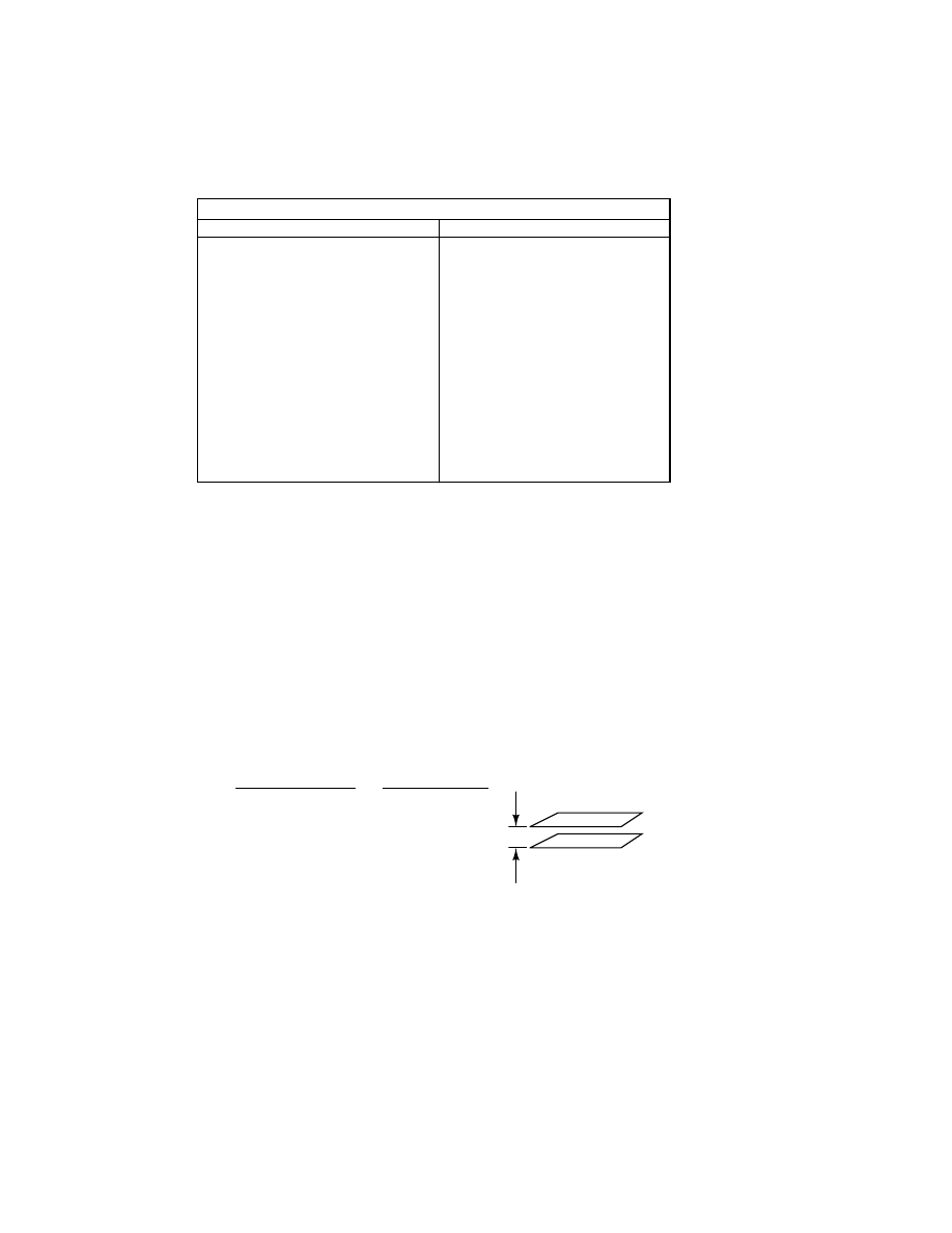
Capacitor sizing equation
Where,
C =
d
ε
A
C =
Capacitance in Farads
ε
=
Permittivity of dielectric (absolute, not
relative)
A =
Area of plate overlap in square meters
d =
Distance between plates in meters
Where,
ε = ε
0
K
ε
0
=
Permittivity of free space
K =
Dielectric constant of material
between plates (see table)
ε
0
=
8.8562 x 10
-12
F/m
1.5. CAPACITOR SIZING EQUATION
5
Dielectric constants
Vacuum
Air
Transformer oil
Wood, oak
Silicones
Ta
2
O
5
Ba
2
TiO
3
1.0000
1.0006
2.5-4
3.3
3.4-4.3
8-10.0
27.6
1200-1500
Dielectric
Dielectric
K
K
Polypropylene
2.0
2.20-2.28
ABS resin
2.4 - 3.2
PTFE, Teflon
Polystyrene
2.45-4.0
Waxed paper
2.5
2.0
Mineral oil
Wood, maple
Glass
4.4
4.9-7.5
Bakelite
3.5-6.0
Quartz, fused
3.8
Mica, muscovite
Poreclain, steatite
Alumina
5.0-8.7
6.5
Castor oil
5.0
Wood, birch
5.2
BaSrTiO
3
Al
2
O
3
7500
Water, distilled
Hard Rubber
2.5-4.8
Glass-bonded mica 6.3-9.3
80
A formula for capacitance in picofards using practical dimensions:
Where,
C =
d
0.0885K(
n-1) A
C = Capacitance in picofarads
K = Dielectric constant
d’
=
Area of one plate in square centimeters
A =
A
’ =
Area of one plate in square inches
d =
Thickness in centimeters
d’ =
Thickness in inches
n =
Number of plates
0.225K(n-1)A’
d
A
6
CHAPTER 1. USEFUL EQUATIONS AND CONVERSION FACTORS
1.6
Inductor sizing equation
Where,
N =
Number of turns in wire coil (straight wire = 1)
L =
N
2
µ
A
l
L =
µ
=
A =
l =
Inductance of coil in Henrys
Permeability of core material (absolute, not relative)
Area of coil in square meters
Average length of coil in meters
µ
=
µ
r
µ
0
µ
r
=
µ
0
=
Relative permeability, dimensionless (
µ
0
=1
for air)
1.26 x 10
-6
T-m/At permeability of free space
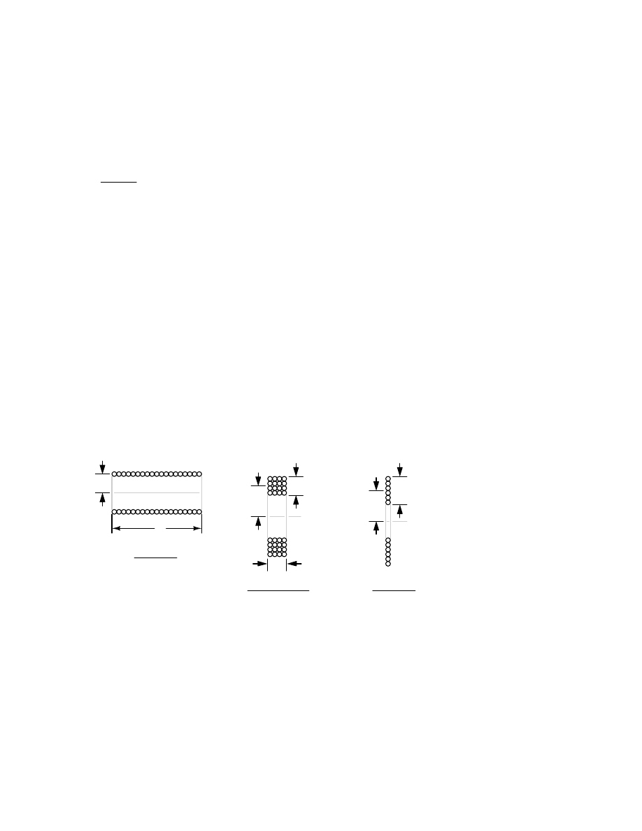
Wheeler’s formulas for inductance of air core coils which follow are usefull for radio frequency
inductors. The following formula for the inductance of a single layer air core solenoid coil is accurate
to approximately 1% for 2r/l < 3. The thick coil formula is 1% accurate when the denominator
terms are approximately equal. Wheeler’s spiral formula is 1% accurate for c>0.2r. While this
is a ”round wire” formula, it may still be applicable to printed circuit spiral inductors at reduced
accuracy.
Where,
N =
Number of turns of wire
L =
N
2
r
2
9r + 10
⋅
l
L =
r =
l =
Inductance of coil in microhenrys
Mean radius of coil in inches
Length of coil in inches
l
r
c = Thickness of coil in inches
r
c
r
c
l
L =
N
2
r
2
L =
0.8N
2
r
2
8r + 11c
6r + 9
⋅
l +
10c
1.7. TIME CONSTANT EQUATIONS
7
The wire table provides ”turns per inch” for enamel magnet wire for use with the inductance
formulas for coils.
AWG
gauge
turns/
inch
AWG
gauge
turns/
inch
AWG
gauge
turns/
inch
10 9.6
11 10.7
12 12.0
13 13.5
14 15.0
15 16.8
16 18.9
17 21.2
18 23.6
19 26.4
20 29.4
21 33.1
22 37.0
23 41.3
24 46.3
25 51.7
26 58.0
27 64.9
28 72.7
29 81.6
30 90.5
31 101
32 113
33 127
34 143
35 158
36 175
37 198
38 224
39 248
AWG
gauge
turns/
inch
40 282
41 327
42 378
43 421
44 471
45 523
46 581
1.7
Time constant equations
1.7.1
Value of time constant in series RC and RL circuits
Time constant in seconds = RC
Time constant in seconds = L/R
1.7.2
Calculating voltage or current at specified time
1 -
1
(Final-Start)
Change =
Universal Time Constant Formula
Where,
Final =
Start =
e =
t =
Value of calculated variable after infinite time
(its ultimate value)
Initial value of calculated variable
Euler’s number ( 2.7182818)
Time in seconds
Time constant for circuit in seconds
e
t/
τ
τ
=

8
CHAPTER 1. USEFUL EQUATIONS AND CONVERSION FACTORS
1.7.3
Calculating time at specified voltage or current
ln
Change
Final - Start
1 -
1
t =
τ
1.8
AC circuit equations
1.8.1
Inductive reactance
X
L
= 2
π
fL
Where,
X
L
=
f =
L =
Inductive reactance in ohms
Frequency in hertz
Inductance in henrys
1.8.2
Capacitive reactance
Where,
f =
Inductive reactance in ohms
Frequency in hertz
X
C
=
2
π
fC
1
X
C
=
C =
Capacitance in farads
1.8.3
Impedance in relation to R and X
Z
L
= R + jX
L
Z
C
= R - jX
C

1.8. AC CIRCUIT EQUATIONS
9
1.8.4
Ohm’s Law for AC
I = E
E
I
Where,
E =
I =
Voltage in volts
Current in amperes (amps)
Z =
Impedance in ohms
E = IZ
Z
Z =
1.8.5
Series and Parallel Impedances
1
1
1
+
+ . . .
1
Z
parallel
=
Z
series
= Z
1
+ Z
2
+ . . . Z
n
Z
1
Z
2
Z
n
NOTE: All impedances must be calculated in complex number form for these equations to work.
1.8.6
Resonance
f
resonant
=
2
π
LC
1
NOTE: This equation applies to a non-resistive LC circuit. In circuits containing resistance as
well as inductance and capacitance, this equation applies only to series configurations and to parallel
configurations where R is very small.

10
CHAPTER 1. USEFUL EQUATIONS AND CONVERSION FACTORS
1.8.7
AC power
P =
true power
P = I
2
R
P =
E
2
R
Q =
reactive power
E
2
X
Measured in units of Watts
Measured in units of Volt-Amps-Reactive (VAR)
S =
apparent power
Q =
Q = I
2
X
S = I
2
Z
E
2
S =
Z
S = IE
Measured in units of Volt-Amps
P = (IE)(
power factor
)
S =
P
2
+ Q
2
Power factor =
cos (Z
phase angle
)
1.9
Decibels
A
V(ratio)
= 10
A
V(dB)
20
20
A
I(ratio)
= 10
A
I(dB)
A
P(ratio)
= 10
A
P(dB)
10
A
V(dB)
= 20 log A
V(ratio)
A
I(dB)
= 20 log A
I(ratio)
A
P(dB)
= 10 log A
P(ratio)

1.10. METRIC PREFIXES AND UNIT CONVERSIONS
11
1.10
Metric prefixes and unit conversions
• Metric prefixes
• Yotta = 10
24
Symbol: Y
• Zetta = 10
21
Symbol: Z
• Exa = 10
18
Symbol: E
• Peta = 10
15
Symbol: P
• Tera = 10
12
Symbol: T
• Giga = 10
9
Symbol: G
• Mega = 10
6
Symbol: M
• Kilo = 10
3
Symbol: k
• Hecto = 10
2
Symbol: h
• Deca = 10
1
Symbol: da
• Deci = 10
−1
Symbol: d
• Centi = 10
−2
Symbol: c
• Milli = 10
−3
Symbol: m
• Micro = 10
−6
Symbol: µ
• Nano = 10
−9
Symbol: n
• Pico = 10
−12
Symbol: p
• Femto = 10
−15
Symbol: f
• Atto = 10
−18
Symbol: a
• Zepto = 10
−21
Symbol: z
• Yocto = 10
−24
Symbol: y
10
0
10
3
10
6
10
9
10
12
10
-3
10
-6
10
-9
10
-12
(none)
kilo
mega
giga
tera
milli
micro
nano
pico
k
M
G
T
m
µ
n
p
10
-2
10
-1
10
1
10
2
deci
centi
deca
hecto
h
da
d
c
METRIC PREFIX SCALE

12
CHAPTER 1. USEFUL EQUATIONS AND CONVERSION FACTORS
• Conversion factors for temperature
•
o
F = (
o
C)(9/5) + 32
•
o
C = (
o
F - 32)(5/9)
•
o
R =
o
F + 459.67
•
o
K =
o
C + 273.15
Conversion equivalencies for volume
1 US gallon (gal) = 231.0 cubic inches (in
3
) = 4 quarts (qt) = 8 pints (pt) = 128
fluid ounces (fl. oz.) = 3.7854 liters (l)
1 Imperial gallon (gal) = 160 fluid ounces (fl. oz.) = 4.546 liters (l)
Conversion equivalencies for distance
1 inch (in) = 2.540000 centimeter (cm)
Conversion equivalencies for velocity
1 mile per hour (mi/h) = 88 feet per minute (ft/m) = 1.46667 feet per second (ft/s)
= 1.60934 kilometer per hour (km/h) = 0.44704 meter per second (m/s) = 0.868976
knot (knot – international)
Conversion equivalencies for weight
1 pound (lb) = 16 ounces (oz) = 0.45359 kilogram (kg)
Conversion equivalencies for force
1 pound-force (lbf) = 4.44822 newton (N)
Acceleration of gravity (free fall), Earth standard
9.806650 meters per second per second (m/s
2
) = 32.1740 feet per second per second
(ft/s
2
)
Conversion equivalencies for area
1 acre = 43560 square feet (ft
2
) = 4840 square yards (yd
2
) = 4046.86 square meters
(m
2
)

1.10. METRIC PREFIXES AND UNIT CONVERSIONS
13
Conversion equivalencies for pressure
1 pound per square inch (psi) = 2.03603 inches of mercury (in. Hg) = 27.6807
inches of water (in. W.C.) = 6894.757 pascals (Pa) = 0.0680460 atmospheres (Atm) =
0.0689476 bar (bar)
Conversion equivalencies for energy or work
1 british thermal unit (BTU – ”International Table”) = 251.996 calories (cal – ”In-
ternational Table”) = 1055.06 joules (J) = 1055.06 watt-seconds (W-s) = 0.293071 watt-
hour (W-hr) = 1.05506 x 10
10
ergs (erg) = 778.169 foot-pound-force (ft-lbf)
Conversion equivalencies for power
1 horsepower (hp – 550 ft-lbf/s) = 745.7 watts (W) = 2544.43 british thermal units
per hour (BTU/hr) = 0.0760181 boiler horsepower (hp – boiler)
Conversion equivalencies for motor torque
Newton-meter
(n-m)
Pound-inch
(lb-in)
Ounce-inch
(oz-in)
Gram-centimeter
(g-cm)
Pound-foot
(lb-ft)
n-m
g-cm
lb-in
lb-ft
oz-in
1
1
1
1
1
141.6
8.85
0.113
7.062 x 10
-3
0.0625
1020
0.738
981 x 10
-6
1.36
115
1383
7.20
8.68 x 10
-3
12
723 x 10
-6
0.0833
5.21 x 10
-3
0.139
16
192
Locate the row corresponding to known unit of torque along the left of the table. Multiply by the
factor under the column for the desired units. For example, to convert 2 oz-in torque to n-m, locate
oz-in row at table left. Locate 7.062 x 10
−3
at intersection of desired n-m units column. Multiply 2
oz-in x (7.062 x 10
−3
) = 14.12 x 10
−3
n-m.
Converting between units is easy if you have a set of equivalencies to work with. Suppose we
wanted to convert an energy quantity of 2500 calories into watt-hours. What we would need to do
is find a set of equivalent figures for those units. In our reference here, we see that 251.996 calories
is physically equal to 0.293071 watt hour. To convert from calories into watt-hours, we must form
a ”unity fraction” with these physically equal figures (a fraction composed of different figures and
different units, the numerator and denominator being physically equal to one another), placing the
desired unit in the numerator and the initial unit in the denominator, and then multiply our initial
value of calories by that fraction.
Since both terms of the ”unity fraction” are physically equal to one another, the fraction as a
whole has a physical value of 1, and so does not change the true value of any figure when multiplied

14
CHAPTER 1. USEFUL EQUATIONS AND CONVERSION FACTORS
by it. When units are canceled, however, there will be a change in units. For example, 2500 calories
multiplied by the unity fraction of (0.293071 w-hr / 251.996 cal) = 2.9075 watt-hours.
2500 calories
1
0.293071 watt-hour
251.996 calories
2.9075 watt-hours
0.293071 watt-hour
251.996 calories
"Unity fraction"
Original figure
2500 calories
. . . cancelling units . . .
Converted figure
The ”unity fraction” approach to unit conversion may be extended beyond single steps. Suppose
we wanted to convert a fluid flow measurement of 175 gallons per hour into liters per day. We have
two units to convert here: gallons into liters, and hours into days. Remember that the word ”per”
in mathematics means ”divided by,” so our initial figure of 175 gallons per hour means 175 gallons
divided by hours. Expressing our original figure as such a fraction, we multiply it by the necessary
unity fractions to convert gallons to liters (3.7854 liters = 1 gallon), and hours to days (1 day = 24
hours). The units must be arranged in the unity fraction in such a way that undesired units cancel
each other out above and below fraction bars. For this problem it means using a gallons-to-liters
unity fraction of (3.7854 liters / 1 gallon) and a hours-to-days unity fraction of (24 hours / 1 day):
1.11. DATA
15
"Unity fraction"
Original figure
. . . cancelling units . . .
Converted figure
175 gallons/hour
1 gallon
3.7854 liters
"Unity fraction"
1 day
24 hours
175 gallons
1 hour
3.7854 liters
1 gallon
24 hours
1 day
15,898.68 liters/day
Our final (converted) answer is 15898.68 liters per day.
1.11
Data
Conversion factors were found in the 78
th
edition of the CRC Handbook of Chemistry and Physics,
and the 3
rd
edition of Bela Liptak’s Instrument Engineers’ Handbook – Process Measurement and
Analysis.
1.12
Contributors
Contributors to this chapter are listed in chronological order of their contributions, from most recent
to first. See Appendix 2 (Contributor List) for dates and contact information.
Gerald Gardner (January 2003): Addition of Imperial gallons conversion.

16
CHAPTER 1. USEFUL EQUATIONS AND CONVERSION FACTORS

Chapter 2
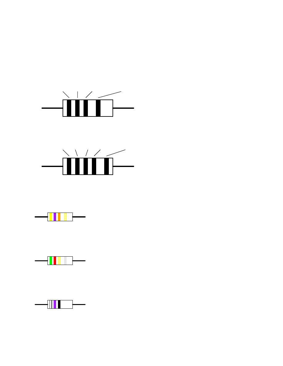
RESISTOR COLOR CODES
Contents
. . . . . . . . . . . . . . . . . . . . . . . . . . . . . . . . . .
18
. . . . . . . . . . . . . . . . . . . . . . . . . . . . . . . . . .
18
. . . . . . . . . . . . . . . . . . . . . . . . . . . . . . . . . .
18
. . . . . . . . . . . . . . . . . . . . . . . . . . . . . . . . . .
19
. . . . . . . . . . . . . . . . . . . . . . . . . . . . . . . . . .
19
. . . . . . . . . . . . . . . . . . . . . . . . . . . . . . . . . .
19
Black
Brown
Red
Orange
Yellow
Green
Blue
Violet
Grey
White
Color
Digit
0
1
2
3
4
5
6
7
8
9
Gold
Silver
(none)
Multiplier
10
0
(1)
10
1
10
2
10
3
10
4
10
5
10
6
10
7
10
8
10
9
10
-1
10
-2
Tolerance (%)
1
2
5
10
20
0.5
0.25
0.1
17
18
CHAPTER 2. RESISTOR COLOR CODES
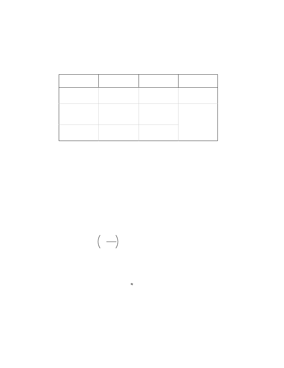
The colors brown, red, green, blue, and violet are used as tolerance codes on 5-band resistors
only. All 5-band resistors use a colored tolerance band. The blank (20%) ”band” is only used with
the ”4-band” code (3 colored bands + a blank ”band”).
Tolerance
Digit Digit Multiplier
4-band code
Digit
Digit
Digit Multiplier Tolerance
5-band code
2.1
Example #1
A resistor colored Yellow-Violet-Orange-Gold would be 47 kΩ with a tolerance of +/- 5%.
2.2
Example #2
A resistor colored Green-Red-Gold-Silver would be 5.2 Ω with a tolerance of +/- 10%.
2.3
Example #3

2.4. EXAMPLE #4
19
A resistor colored White-Violet-Black would be 97 Ω with a tolerance of +/- 20%. When you
see only three color bands on a resistor, you know that it is actually a 4-band code with a blank
(20%) tolerance band.
2.4
Example #4
A resistor colored Orange-Orange-Black-Brown-Violet would be 3.3 kΩ with a tolerance of +/-
0.1%.
2.5
Example #5
A resistor colored Brown-Green-Grey-Silver-Red would be 1.58 Ω with a tolerance of +/- 2%.
2.6
Example #6
A resistor colored Blue-Brown-Green-Silver-Blue would be 6.15 Ω with a tolerance of +/- 0.25%.

20
CHAPTER 2. RESISTOR COLOR CODES

Chapter 3
CONDUCTOR AND
INSULATOR TABLES
Contents
. . . . . . . . . . . . . . . . . . . . . . . . . . . .
21
. . . . . . . . . . . . . . . . . . . . . . . . .
22
Coefficients of specific resistance
. . . . . . . . . . . . . . . . . . . . . .
23
Temperature coefficients of resistance
. . . . . . . . . . . . . . . . . . .
24
Critical temperatures for superconductors
. . . . . . . . . . . . . . . .
24
Dielectric strengths for insulators
. . . . . . . . . . . . . . . . . . . . .
25
. . . . . . . . . . . . . . . . . . . . . . . . . . . . . . . . . . . . . . .
25
3.1
Copper wire gage table
Soild copper wire table:
Size
Diameter
Cross-sectional area
Weight
AWG
inches
cir. mils
sq. inches
lb/1000 ft
================================================================
4/0 -------- 0.4600 ------- 211,600 ------ 0.1662 ------ 640.5
3/0 -------- 0.4096 ------- 167,800 ------ 0.1318 ------ 507.9
2/0 -------- 0.3648 ------- 133,100 ------ 0.1045 ------ 402.8
1/0 -------- 0.3249 ------- 105,500 ----- 0.08289 ------ 319.5
1 ---------- 0.2893 ------- 83,690 ------ 0.06573 ------ 253.5
2 ---------- 0.2576 ------- 66,370 ------ 0.05213 ------ 200.9
3 ---------- 0.2294 ------- 52,630 ------ 0.04134 ------ 159.3
4 ---------- 0.2043 ------- 41,740 ------ 0.03278 ------ 126.4
5 ---------- 0.1819 ------- 33,100 ------ 0.02600 ------ 100.2
6 ---------- 0.1620 ------- 26,250 ------ 0.02062 ------ 79.46
7 ---------- 0.1443 ------- 20,820 ------ 0.01635 ------ 63.02
21

22
CHAPTER 3. CONDUCTOR AND INSULATOR TABLES
8 ---------- 0.1285 ------- 16,510 ------ 0.01297 ------ 49.97
9 ---------- 0.1144 ------- 13,090 ------ 0.01028 ------ 39.63
10 --------- 0.1019 ------- 10,380 ------ 0.008155 ----- 31.43
11 --------- 0.09074 ------- 8,234 ------ 0.006467 ----- 24.92
12 --------- 0.08081 ------- 6,530 ------ 0.005129 ----- 19.77
13 --------- 0.07196 ------- 5,178 ------ 0.004067 ----- 15.68
14 --------- 0.06408 ------- 4,107 ------ 0.003225 ----- 12.43
15 --------- 0.05707 ------- 3,257 ------ 0.002558 ----- 9.858
16 --------- 0.05082 ------- 2,583 ------ 0.002028 ----- 7.818
17 --------- 0.04526 ------- 2,048 ------ 0.001609 ----- 6.200
18 --------- 0.04030 ------- 1,624 ------ 0.001276 ----- 4.917
19 --------- 0.03589 ------- 1,288 ------ 0.001012 ----- 3.899
20 --------- 0.03196 ------- 1,022 ----- 0.0008023 ----- 3.092
21 --------- 0.02846 ------- 810.1 ----- 0.0006363 ----- 2.452
22 --------- 0.02535 ------- 642.5 ----- 0.0005046 ----- 1.945
23 --------- 0.02257 ------- 509.5 ----- 0.0004001 ----- 1.542
24 --------- 0.02010 ------- 404.0 ----- 0.0003173 ----- 1.233
25 --------- 0.01790 ------- 320.4 ----- 0.0002517 ----- 0.9699
26 --------- 0.01594 ------- 254.1 ----- 0.0001996 ----- 0.7692
27 --------- 0.01420 ------- 201.5 ----- 0.0001583 ----- 0.6100
28 --------- 0.01264 ------- 159.8 ----- 0.0001255 ----- 0.4837
29 --------- 0.01126 ------- 126.7 ----- 0.00009954 ---- 0.3836
30 --------- 0.01003 ------- 100.5 ----- 0.00007894 ---- 0.3042
31 -------- 0.008928 ------- 79.70 ----- 0.00006260 ---- 0.2413
32 -------- 0.007950 ------- 63.21 ----- 0.00004964 ---- 0.1913
33 -------- 0.007080 ------- 50.13 ----- 0.00003937 ---- 0.1517
34 -------- 0.006305 ------- 39.75 ----- 0.00003122 ---- 0.1203
35 -------- 0.005615 ------- 31.52 ----- 0.00002476 --- 0.09542
36 -------- 0.005000 ------- 25.00 ----- 0.00001963 --- 0.07567
37 -------- 0.004453 ------- 19.83 ----- 0.00001557 --- 0.06001
38 -------- 0.003965 ------- 15.72 ----- 0.00001235 --- 0.04759
39 -------- 0.003531 ------- 12.47 ---- 0.000009793 --- 0.03774
40 -------- 0.003145 ------- 9.888 ---- 0.000007766 --- 0.02993
41 -------- 0.002800 ------- 7.842 ---- 0.000006159 --- 0.02374
42 -------- 0.002494 ------- 6.219 ---- 0.000004884 --- 0.01882
43 -------- 0.002221 ------- 4.932 ---- 0.000003873 --- 0.01493
44 -------- 0.001978 ------- 3.911 ---- 0.000003072 --- 0.01184
3.2
Copper wire ampacity table
Ampacities of copper wire, in free air at 30
o
C:
========================================================
|
INSULATION TYPE:
|
|
RUW, T
THW, THWN
FEP, FEPB
|
|
TW
RUH
THHN, XHHW
|

3.3. COEFFICIENTS OF SPECIFIC RESISTANCE
23
========================================================
Size
Current Rating
Current Rating
Current Rating
AWG
@ 60 degrees C
@ 75 degrees C
@ 90 degrees C
========================================================
20 -------- *9 ----------------------------- *12.5
18 -------- *13 ------------------------------ 18
16 -------- *18 ------------------------------ 24
14 --------- 25 ------------- 30 ------------- 35
12 --------- 30 ------------- 35 ------------- 40
10 --------- 40 ------------- 50 ------------- 55
8 ---------- 60 ------------- 70 ------------- 80
6 ---------- 80 ------------- 95 ------------ 105
4 --------- 105 ------------ 125 ------------ 140
2 --------- 140 ------------ 170 ------------ 190
1 --------- 165 ------------ 195 ------------ 220
1/0 ------- 195 ------------ 230 ------------ 260
2/0 ------- 225 ------------ 265 ------------ 300
3/0 ------- 260 ------------ 310 ------------ 350
4/0 ------- 300 ------------ 360 ------------ 405
*
= estimated values; normally, wire gages this small are not manufactured with these insulation
types.
3.3
Coefficients of specific resistance
Specific resistance at 20
o
C:
Material
Element/Alloy
(ohm-cmil/ft)
(ohm-cm)
====================================================================
Nichrome ------- Alloy ---------------- 675 ------------- 112.2
−6
Nichrome V ----- Alloy ---------------- 650 ------------- 108.1
−6
Manganin ------- Alloy ---------------- 290 ------------- 48.21
−6
Constantan ----- Alloy ---------------- 272.97 ---------- 45.38
−6
Steel* --------- Alloy ---------------- 100 ------------- 16.62
−6
Platinum ------ Element --------------- 63.16 ----------- 10.5
−6
Iron ---------- Element --------------- 57.81 ----------- 9.61
−6
Nickel -------- Element --------------- 41.69 ----------- 6.93
−6
Zinc ---------- Element --------------- 35.49 ----------- 5.90
−6
Molybdenum ---- Element --------------- 32.12 ----------- 5.34
−6
Tungsten ------ Element --------------- 31.76 ----------- 5.28
−6
Aluminum ------ Element --------------- 15.94 ----------- 2.650
−6
Gold ---------- Element --------------- 13.32 ----------- 2.214
−6
Copper -------- Element --------------- 10.09 ----------- 1.678
−6
Silver -------- Element --------------- 9.546 ----------- 1.587
−6
*
= Steel alloy at 99.5 percent iron, 0.5 percent carbon.

24
CHAPTER 3. CONDUCTOR AND INSULATOR TABLES
3.4
Temperature coefficients of resistance
Temperature coefficient (α) per degree C:
Material
Element/Alloy
Temp. coefficient
=====================================================
Nickel -------- Element --------------- 0.005866
Iron ---------- Element --------------- 0.005671
Molybdenum ---- Element --------------- 0.004579
Tungsten ------ Element --------------- 0.004403
Aluminum ------ Element --------------- 0.004308
Copper -------- Element --------------- 0.004041
Silver -------- Element --------------- 0.003819
Platinum ------ Element --------------- 0.003729
Gold ---------- Element --------------- 0.003715
Zinc ---------- Element --------------- 0.003847
Steel* --------- Alloy ---------------- 0.003
Nichrome ------- Alloy ---------------- 0.00017
Nichrome V ----- Alloy ---------------- 0.00013
Manganin ------- Alloy ------------ +/- 0.000015
Constantan ----- Alloy --------------- -0.000074
*
= Steel alloy at 99.5 percent iron, 0.5 percent carbon
3.5
Critical temperatures for superconductors
Critical temperatures given in degrees Kelvin:
Material
Element/Alloy
Critical temperature
======================================================
Aluminum -------- Element --------------- 1.20
Cadmium --------- Element --------------- 0.56
Lead ------------ Element --------------- 7.2
Mercury --------- Element --------------- 4.16
Niobium --------- Element --------------- 8.70
Thorium --------- Element --------------- 1.37
Tin ------------- Element --------------- 3.72
Titanium -------- Element --------------- 0.39
Uranium --------- ELement --------------- 1.0
Zinc ------------ Element --------------- 0.91
Niobium/Tin ------ Alloy ---------------- 18.1
Cupric sulphide - Compound -------------- 1.6
Note: all critical temperatures given at zero magnetic field strength.

3.6. DIELECTRIC STRENGTHS FOR INSULATORS
25
3.6
Dielectric strengths for insulators
Dielectric strength in kilovolts per inch (kV/in):
Material*
Dielectric strength
=========================================
Vacuum --------------------- 20
Air ------------------------ 20 to 75
Porcelain ------------------ 40 to 200
Paraffin Wax --------------- 200 to 300
Transformer Oil ------------ 400
Bakelite ------------------- 300 to 550
Rubber --------------------- 450 to 700
Shellac -------------------- 900
Paper ---------------------- 1250
Teflon --------------------- 1500
Glass ---------------------- 2000 to 3000
Mica ----------------------- 5000
*
= Materials listed are specially prepared for electrical use
3.7
Data
Tables of specific resistance and temperature coefficient of resistance for elemental materials (not
alloys) were derived from figures found in the 78th edition of the CRC Handbook of Chemistry and
Physics. Superconductivity data from Collier’s Encyclopedia (volume 21, 1968, page 640).

26
CHAPTER 3. CONDUCTOR AND INSULATOR TABLES

Chapter 4
ALGEBRA REFERENCE
Contents
. . . . . . . . . . . . . . . . . . . . . . . . . . . . . . . . .
28
. . . . . . . . . . . . . . . . . . . . . . . . . . . . .
28
. . . . . . . . . . . . . . . . . . . . . . . . . . . .
28
. . . . . . . . . . . . . . . . . . . . . . . . . .
28
. . . . . . . . . . . . . . . . . . . . . . . . . . .
28
. . . . . . . . . . . . . . . . . . . . . . . . . . . .
28
. . . . . . . . . . . . . . . . . . . . . . . . . . . . . . . . . . . . .
29
. . . . . . . . . . . . . . . . . . . . . . . . . . . . .
29
. . . . . . . . . . . . . . . . . . . . . . . . . . . . . .
29
. . . . . . . . . . . . . . . . . . . . . . . . . . . . . .
29
. . . . . . . . . . . . . . . . . . . . . . . . . . . . . . . . .
29
. . . . . . . . . . . . . . . . . . . . . . . . . . . . . . . . . . . . . . . .
30
. . . . . . . . . . . . . . . . . . . . . . . . . . . . . . . . . . .
30
. . . . . . . . . . . . . . . . . . . . . . . . . . . .
30
. . . . . . . . . . . . . . . . . . . . . . . . . . . .
31
. . . . . . . . . . . . . . . . . . . . . . . . . . . .
31
. . . . . . . . . . . . . . . . . . . . . . . . . . . .
32
. . . . . . . . . . . . . . . . . . . . . . . . . . . . . . . . . . . .
32
. . . . . . . . . . . . . . . . . . . . . . . . . . . . . .
32
. . . . . . . . . . . . . . . . . . . . . . . . . . . . . .
33
. . . . . . . . . . . . . . . . . . . . . . . . . . . . . . . . . . . .
33
4.10.1 Definition of a factorial
. . . . . . . . . . . . . . . . . . . . . . . . . . . .
33
. . . . . . . . . . . . . . . . . . . . . . . . . . . . . . . .
33
4.11 Solving simultaneous equations
. . . . . . . . . . . . . . . . . . . . . . .
33
. . . . . . . . . . . . . . . . . . . . . . . . . . . . . .
34
. . . . . . . . . . . . . . . . . . . . . . . . . . . . . . . .
38
. . . . . . . . . . . . . . . . . . . . . . . . . . . . . . . . . .
43
27

28
CHAPTER 4. ALGEBRA REFERENCE
4.1
Basic identities
a + 0 = a
1a = a
0a = 0
a
1
= a
a
0 = 0
a
a = 1
a
0
=
undefined
Note: while division by zero is popularly thought to be equal to infinity, this is not technically
true. In some practical applications it may be helpful to think the result of such a fraction approach-
ing infinity as the denominator approaches zero (imagine calculating current I=E/R in a circuit with
resistance approaching zero – current would approach infinity), but the actual fraction of anything
divided by zero is undefined in the scope of ”real” numbers.
4.2
Arithmetic properties
4.2.1
The associative property
In addition and multiplication, terms may be arbitrarily associated with each other through the use
of parentheses:
a + (b + c) = (a + b) + c
a(bc) = (ab)c
4.2.2
The commutative property
In addition and multiplication, terms may be arbitrarily interchanged, or commutated :
a + b = b + a
ab=ba
4.2.3
The distributive property
a(b + c) = ab + ac
4.3
Properties of exponents
a
m
a
n
= a
m+n
(ab)
m
= a
m
b
m
(a
m
)
n
= a
mn
a
m
a
n
= a
m-n
4.4. RADICALS
29
4.4
Radicals
4.4.1
Definition of a radical
When people talk of a ”square root,” they’re referring to a radical with a root of 2. This is math-
ematically equivalent to a number raised to the power of 1/2. This equivalence is useful to know
when using a calculator to determine a strange root. Suppose for example you needed to find the
fourth root of a number, but your calculator lacks a ”4th root” button or function. If it has a y
x
function (which any scientific calculator should have), you can find the fourth root by raising that
number to the 1/4 power, or x
0.25
.
x
a
= a
1/x
It is important to remember that when solving for an even root (square root, fourth root, etc.)
of any number, there are two valid answers. For example, most people know that the square root of
nine is three, but negative three is also a valid answer, since (-3)
2
= 9 just as 3
2
= 9.
4.4.2
Properties of radicals
x
a
x
= a
x
= a
a
x
x
ab
=
a
b
x
x
x
a
b
=
x
a
x
b
4.5
Important constants
4.5.1
Euler’s number
Euler’s constant is an important value for exponential functions, especially scientific applications
involving decay (such as the decay of a radioactive substance). It is especially important in calculus
due to its uniquely self-similar properties of integration and differentiation.
e approximately equals:
2.71828 18284 59045 23536 02874 71352 66249 77572 47093 69996

30
CHAPTER 4. ALGEBRA REFERENCE
e =
k = 0
1
k!
1
0! +
1
+
1
+
1
+
1
. . .
1!
2!
3!
n!
4.5.2
Pi
Pi (π) is defined as the ratio of a circle’s circumference to its diameter.
Pi approximately equals:
3.14159 26535 89793 23846 26433 83279 50288 41971 69399 37511
Note: For both Euler’s constant (e) and pi (π), the spaces shown between each set of five digits
have no mathematical significance. They are placed there just to make it easier for your eyes to
”piece” the number into five-digit groups when manually copying.
4.6
Logarithms
4.6.1
Definition of a logarithm
log
b
x = y
b
y
= x
If:
Then:
Where,
b =
"Base" of the logarithm
”log” denotes a common logarithm (base = 10), while ”ln” denotes a natural logarithm (base =
e).
4.7. FACTORING EQUIVALENCIES
31
4.6.2
Properties of logarithms
(log a) + (log b) = log ab
(log a) - (log b) = log a
b
log a
m
= (m)(log a)
a
(log m)
= m
These properties of logarithms come in handy for performing complex multiplication and division
operations. They are an example of something called a transform function, whereby one type of
mathematical operation is transformed into another type of mathematical operation that is simpler
to solve. Using a table of logarithm figures, one can multiply or divide numbers by adding or
subtracting their logarithms, respectively. then looking up that logarithm figure in the table and
seeing what the final product or quotient is.
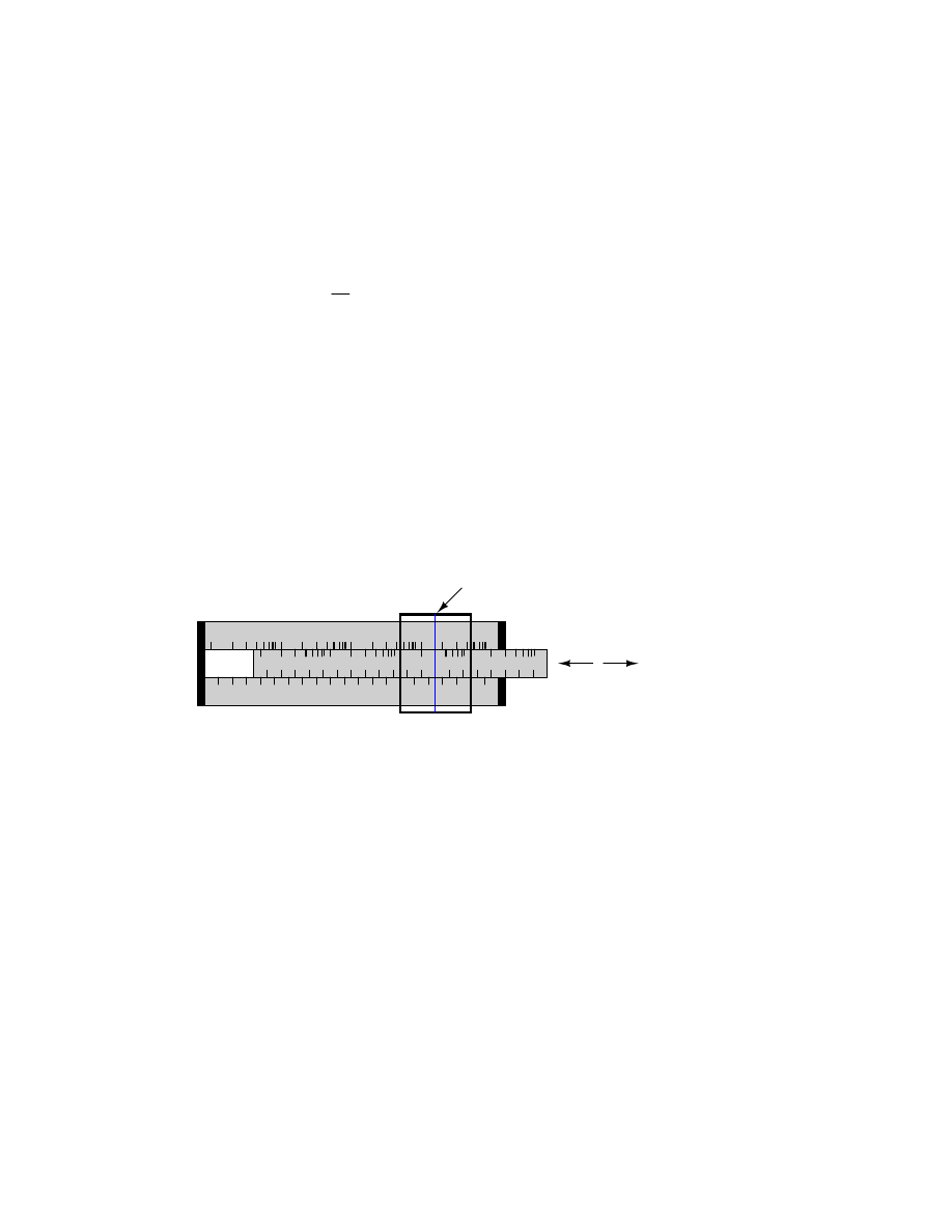
Slide rules work on this principle of logarithms by performing multiplication and division through
addition and subtraction of distances on the slide.
Numerical quantities are represented by
the positioning of the slide.
Slide
Slide rule
Cursor
Marks on a slide rule’s scales are spaced in a logarithmic fashion, so that a linear positioning of
the scale or cursor results in a nonlinear indication as read on the scale(s). Adding or subtracting
lengths on these logarithmic scales results in an indication equivalent to the product or quotient,
respectively, of those lengths.
Most slide rules were also equipped with special scales for trigonometric functions, powers, roots,
and other useful arithmetic functions.
4.7
Factoring equivalencies
x
2
- y
2
= (x+y)(x-y)
x
3
- y
3
= (x-y)(x
2
+ xy + y
2
)

32
CHAPTER 4. ALGEBRA REFERENCE
4.8
The quadratic formula
-b +
-
b
2
- 4ac
2a
x =
For a polynomial expression in
the form of:
ax
2
+ bx + c = 0
4.9
Sequences
4.9.1
Arithmetic sequences
An arithmetic sequence is a series of numbers obtained by adding (or subtracting) the same value
with each step. A child’s counting sequence (1, 2, 3, 4, . . .) is a simple arithmetic sequence, where
the common difference is 1: that is, each adjacent number in the sequence differs by a value of one.
An arithmetic sequence counting only even numbers (2, 4, 6, 8, . . .) or only odd numbers (1, 3, 5,
7, 9, . . .) would have a common difference of 2.
In the standard notation of sequences, a lower-case letter ”a” represents an element (a single
number) in the sequence. The term ”a
n
” refers to the element at the n
th
step in the sequence. For
example, ”a
3
” in an even-counting (common difference = 2) arithmetic sequence starting at 2 would
be the number 6, ”a” representing 4 and ”a
1
” representing the starting point of the sequence (given
in this example as 2).
A capital letter ”A” represents the sum of an arithmetic sequence. For instance, in the same
even-counting sequence starting at 2, A
4
is equal to the sum of all elements from a
1
through a
4
,
which of course would be 2 + 4 + 6 + 8, or 20.
a
n
= a
n-1
+ d
Where:
d =
The "common difference"
a
n
= a
1
+ d(n-1)
Example of an arithmetic sequence:
A
n
= a
1
+ a
2
+ . . . a
n
A
n
=
n
2
(a
1
+ a
n
)
-7, -3, 1, 5, 9, 13, 17, 21, 25 . . .

4.10. FACTORIALS
33
4.9.2
Geometric sequences
A geometric sequence, on the other hand, is a series of numbers obtained by multiplying (or dividing)
by the same value with each step. A binary place-weight sequence (1, 2, 4, 8, 16, 32, 64, . . .) is
a simple geometric sequence, where the common ratio is 2: that is, each adjacent number in the
sequence differs by a factor of two.
Where:
A
n
= a
1
+ a
2
+ . . . a
n
a
n
= r(a
n-1
)
a
n
= a
1
(r
n-1
)
r =
The "common ratio"
Example of a geometric sequence:
3, 12, 48, 192, 768, 3072 . . .
A
n
=
a
1
(1 - r
n
)
1 - r
4.10
Factorials
4.10.1
Definition of a factorial
Denoted by the symbol ”!” after an integer; the product of that integer and all integers in descent
to 1.
Example of a factorial:
5! = 5
x
4
x
3
x
2
x 1
5! = 120
4.10.2
Strange factorials
0! = 1
1! = 1
4.11
Solving simultaneous equations
The terms simultaneous equations and systems of equations refer to conditions where two or more
unknown variables are related to each other through an equal number of equations. Consider the
following example:
34
CHAPTER 4. ALGEBRA REFERENCE
x + y = 24
2x - y = -6
For this set of equations, there is but a single combination of values for x and y that will satisfy
both. Either equation, considered separately, has an infinitude of valid (x,y) solutions, but together
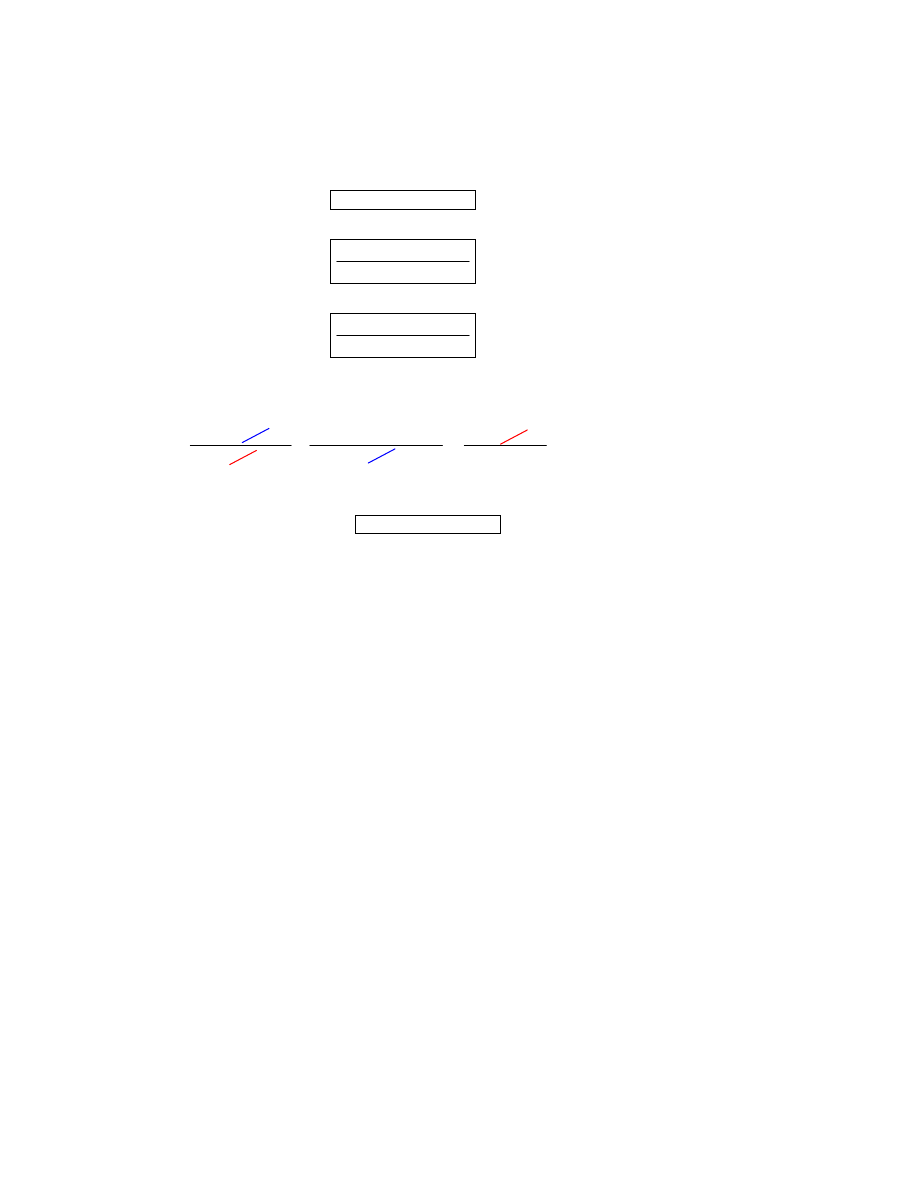
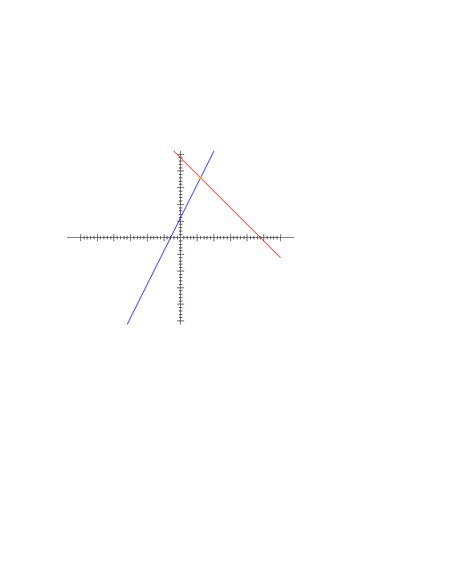
there is only one. Plotted on a graph, this condition becomes obvious:
x + y = 24
2x - y = -6
(6,18)
Each line is actually a continuum of points representing possible x and y solution pairs for each
equation. Each equation, separately, has an infinite number of ordered pair (x,y) solutions. There is
only one point where the two linear functions x + y = 24 and 2x - y = -6 intersect (where one of
their many independent solutions happen to work for both equations), and that is where x is equal
to a value of 6 and y is equal to a value of 18.
Usually, though, graphing is not a very efficient way to determine the simultaneous solution set
for two or more equations. It is especially impractical for systems of three or more variables. In a
three-variable system, for example, the solution would be found by the point intersection of three
planes in a three-dimensional coordinate space – not an easy scenario to visualize.
4.11.1
Substitution method
Several algebraic techniques exist to solve simultaneous equations. Perhaps the easiest to compre-
hend is the substitution method. Take, for instance, our two-variable example problem:
x + y = 24
2x - y = -6
In the substitution method, we manipulate one of the equations such that one variable is defined
in terms of the other:

4.11. SOLVING SIMULTANEOUS EQUATIONS
35
x + y = 24
y = 24 - x
Defining
y
in terms of
x
Then, we take this new definition of one variable and substitute it for the same variable in the
other equation. In this case, we take the definition of y, which is 24 - x and substitute this for the
y
term found in the other equation:
y = 24 - x
2x - y = -6
substitute
2x - (24 - x) = -6
Now that we have an equation with just a single variable (x), we can solve it using ”normal”
algebraic techniques:
2x - (24 - x) = -6
2x - 24 + x = -6
3x -24 = -6
Distributive property
Combining like terms
Adding 24 to each side
3x = 18
Dividing both sides by 3
x = 6
Now that x is known, we can plug this value into any of the original equations and obtain a value
for y. Or, to save us some work, we can plug this value (6) into the equation we just generated to
define y in terms of x, being that it is already in a form to solve for y:
36
CHAPTER 4. ALGEBRA REFERENCE
y = 24 - x
substitute
x = 6
y = 24 - 6
y = 18
Applying the substitution method to systems of three or more variables involves a similar pattern,
only with more work involved. This is generally true for any method of solution: the number of
steps required for obtaining solutions increases rapidly with each additional variable in the system.
To solve for three unknown variables, we need at least three equations. Consider this example:
x - y + z = 10
3x + y + 2z = 34
-5x + 2y - z = -14
Being that the first equation has the simplest coefficients (1, -1, and 1, for x, y, and z, respec-
tively), it seems logical to use it to develop a definition of one variable in terms of the other two. In
this example, I’ll solve for x in terms of y and z:
x - y + z = 10
x = y - z + 10
Adding
y
and subtracting
z
from both sides
Now, we can substitute this definition of x where x appears in the other two equations:
3x + y + 2z = 34
-5x + 2y - z = -14
x = y - z + 10
substitute
3(y - z + 10) + y + 2z = 34
substitute
x = y - z + 10
-5(y - z + 10) + 2y - z = -14
Reducing these two equations to their simplest forms:
4.11. SOLVING SIMULTANEOUS EQUATIONS
37
3(y - z + 10) + y + 2z = 34
-5(y - z + 10) + 2y - z = -14
3y - 3z + 30 + y + 2z = 34
-5y + 5z - 50 + 2y - z = -14
-3y + 4z - 50 = -14
-3y + 4z = 36
Distributive property
Combining like terms
Moving constant values to right
of the "=" sign
4y - z + 30 = 34
4y - z = 4
So far, our efforts have reduced the system from three variables in three equations to two variables
in two equations. Now, we can apply the substitution technique again to the two equations 4y - z
= 4
and -3y + 4z = 36 to solve for either y or z. First, I’ll manipulate the first equation to define
z
in terms of y:
4y - z = 4
z = 4y - 4
Adding
z
to both sides;
subtracting
4
from both sides
Next, we’ll substitute this definition of z in terms of y where we see z in the other equation:
z = 4y - 4
-3y + 4z = 36
substitute
-3y + 4(4y - 4) = 36
-3y + 16y - 16 = 36
13y - 16 = 36
13y = 52
y = 4
Distributive property
Combining like terms
Adding
16
to both sides
Dividing both sides by
13
38
CHAPTER 4. ALGEBRA REFERENCE
Now that y is a known value, we can plug it into the equation defining z in terms of y and obtain
a figure for z:
z = 4y - 4
substitute
y = 4
z = 16 - 4
z = 12
Now, with values for y and z known, we can plug these into the equation where we defined x in
terms of y and z, to obtain a value for x:
x = y - z + 10
y = 4
z = 12
x = 4 - 12 + 10
x = 2
substitute
substitute
In closing, we’ve found values for x, y, and z of 2, 4, and 12, respectively, that satisfy all three
equations.
4.11.2
Addition method
While the substitution method may be the easiest to grasp on a conceptual level, there are other
methods of solution available to us. One such method is the so-called addition method, whereby
equations are added to one another for the purpose of canceling variable terms.
Let’s take our two-variable system used to demonstrate the substitution method:
x + y = 24
2x - y = -6
One of the most-used rules of algebra is that you may perform any arithmetic operation you wish
to an equation so long as you do it equally to both sides. With reference to addition, this means we
may add any quantity we wish to both sides of an equation – so long as it’s the same quantity –
without altering the truth of the equation.

4.11. SOLVING SIMULTANEOUS EQUATIONS
39
An option we have, then, is to add the corresponding sides of the equations together to form a
new equation. Since each equation is an expression of equality (the same quantity on either side
of the = sign), adding the left-hand side of one equation to the left-hand side of the other equation
is valid so long as we add the two equations’ right-hand sides together as well. In our example
equation set, for instance, we may add x + y to 2x - y, and add 24 and -6 together as well to form
a new equation. What benefit does this hold for us? Examine what happens when we do this to our
example equation set:
x + y = 24
2x - y = -6
+
3x + 0 = 18
Because the top equation happened to contain a positive y term while the bottom equation
happened to contain a negative y term, these two terms canceled each other in the process of
addition, leaving no y term in the sum. What we have left is a new equation, but one with only a
single unknown variable, x! This allows us to easily solve for the value of x:
3x + 0 = 18
3x = 18
x = 6
Dropping the
0
term
Dividing both sides by
3
Once we have a known value for x, of course, determining y’s value is a simply matter of sub-
stitution (replacing x with the number 6) into one of the original equations. In this example, the
technique of adding the equations together worked well to produce an equation with a single un-
known variable. What about an example where things aren’t so simple? Consider the following
equation set:
2x + 2y = 14
3x + y = 13
We could add these two equations together – this being a completely valid algebraic operation –
but it would not profit us in the goal of obtaining values for x and y:
2x + 2y = 14
3x + y = 13
+
5x + 3y = 27
The resulting equation still contains two unknown variables, just like the original equations do,
and so we’re no further along in obtaining a solution. However, what if we could manipulate one
of the equations so as to have a negative term that would cancel the respective term in the other
equation when added? Then, the system would reduce to a single equation with a single unknown
variable just as with the last (fortuitous) example.

40
CHAPTER 4. ALGEBRA REFERENCE
If we could only turn the y term in the lower equation into a - 2y term, so that when the two
equations were added together, both y terms in the equations would cancel, leaving us with only
an x term, this would bring us closer to a solution. Fortunately, this is not difficult to do. If we
multiply each and every term of the lower equation by a -2, it will produce the result we seek:
-2(3x + y) = -2(13)
-6x - 2y = -26
Distributive property
Now, we may add this new equation to the original, upper equation:
-6x - 2y = -26
2x + 2y = 14
+
-4x + 0y = -12
Solving for x, we obtain a value of 3:
-4x + 0y = -12
Dropping the
0
term
-4x = -12
x = 3
Dividing both sides by
-4
Substituting this new-found value for x into one of the original equations, the value of y is easily
determined:
x = 3
2x + 2y = 14
substitute
6 + 2y = 14
2y = 8
Subtracting
6
from both sides
y = 4
Dividing both sides by
2
Using this solution technique on a three-variable system is a bit more complex. As with substi-
tution, you must use this technique to reduce the three-equation system of three variables down to

4.11. SOLVING SIMULTANEOUS EQUATIONS
41
two equations with two variables, then apply it again to obtain a single equation with one unknown
variable. To demonstrate, I’ll use the three-variable equation system from the substitution section:
x - y + z = 10
3x + y + 2z = 34
-5x + 2y - z = -14
Being that the top equation has coefficient values of 1 for each variable, it will be an easy equation
to manipulate and use as a cancellation tool. For instance, if we wish to cancel the 3x term from
the middle equation, all we need to do is take the top equation, multiply each of its terms by -3,
then add it to the middle equation like this:
x - y + z = 10
3x + y + 2z = 34
-3(x - y + z) = -3(10)
Multiply both sides by
-3
-3x + 3y - 3z = -30
-3x + 3y - 3z = -30
+
0x + 4y - z = 4
or
4y - z = 4
(Adding)
Distributive property
We can rid the bottom equation of its -5x term in the same manner: take the original top
equation, multiply each of its terms by 5, then add that modified equation to the bottom equation,
leaving a new equation with only y and z terms:

42
CHAPTER 4. ALGEBRA REFERENCE
x - y + z = 10
+
or
(Adding)
Multiply both sides by
5
5(x - y + z) = 5(10)
5x - 5y + 5z = 50
Distributive property
5x - 5y + 5z = 50
-5x + 2y - z = -14
0x - 3y + 4z = 36
-3y + 4z = 36
At this point, we have two equations with the same two unknown variables, y and z:
-3y + 4z = 36
4y - z = 4
By inspection, it should be evident that the -z term of the upper equation could be leveraged
to cancel the 4z term in the lower equation if only we multiply each term of the upper equation by
4
and add the two equations together:
-3y + 4z = 36
4y - z = 4
4(4y - z) = 4(4)
Multiply both sides by
4
Distributive property
16y - 4z = 16
16y - 4z = 16
+
(Adding)
13y + 0z = 52
or
13y = 52
Taking the new equation 13y = 52 and solving for y (by dividing both sides by 13), we get a
value of 4 for y. Substituting this value of 4 for y in either of the two-variable equations allows us to

4.12. CONTRIBUTORS
43
solve for z. Substituting both values of y and z into any one of the original, three-variable equations
allows us to solve for x. The final result (I’ll spare you the algebraic steps, since you should be
familiar with them by now!) is that x = 2, y = 4, and z = 12.
4.12
Contributors
Contributors to this chapter are listed in chronological order of their contributions, from most recent
to first. See Appendix 2 (Contributor List) for dates and contact information.
Chirvasuta Constantin (April 2, 2003): Pointed out error in quadratic equation formula.

44
CHAPTER 4. ALGEBRA REFERENCE

Chapter 5
TRIGONOMETRY REFERENCE
Contents
. . . . . . . . . . . . . . . . . . . . . . . . .
45
. . . . . . . . . . . . . . . . . . . . . . . . . . . .
46
. . . . . . . . . . . . . . . . . . . . . . . . . . .
46
Non-right triangle trigonometry
. . . . . . . . . . . . . . . . . . . . . .
46
The Law of Sines (for any triangle)
. . . . . . . . . . . . . . . . . . . . . .
46
The Law of Cosines (for any triangle)
. . . . . . . . . . . . . . . . . . . .
47
. . . . . . . . . . . . . . . . . . . . . . . . .
47
. . . . . . . . . . . . . . . . . . . . . . . . . . . . .
47
. . . . . . . . . . . . . . . . . . . . . . . . . . . . . . . . . .
47
5.1
Right triangle trigonometry
Adjacent (A)
Opposite (O)
Hypotenuse (H)
Angle
x
90
o
A right triangle is defined as having one angle precisely equal to 90
o
(a right angle).
45

46
CHAPTER 5. TRIGONOMETRY REFERENCE
5.1.1
Trigonometric identities
sin x = O
H
cos x =
H
A
tan x = O
A
csc x =
O
H
sec x =
A
H
cot x =
O
A
tan x =
sin x
cos x
sin x
cos x
cot x =
H is the Hypotenuse, always being opposite the right angle. Relative to angle x, O is the Opposite
and A is the Adjacent.
”Arc” functions such as ”arcsin”, ”arccos”, and ”arctan” are the complements of normal trigono-
metric functions. These functions return an angle for a ratio input. For example, if the tangent of
45
o
is equal to 1, then the ”arctangent” (arctan) of 1 is 45
o
. ”Arc” functions are useful for finding
angles in a right triangle if the side lengths are known.
5.1.2
The Pythagorean theorem
H
2
= A
2
+ O
2
5.2
Non-right triangle trigonometry
A
B
C
a
b
c
5.2.1
The Law of Sines (for any triangle)
sin a
A
=
=
sin b
B
sin c
C

5.3. TRIGONOMETRIC EQUIVALENCIES
47
5.2.2
The Law of Cosines (for any triangle)
A
2
= B
2
+ C
2
- (2BC)(cos a)
B
2
= A
2
+ C
2
- (2AC)(cos b)
C
2
= A
2
+ B
2
- (2AB)(cos c)
5.3
Trigonometric equivalencies
sin -x = -sin x
cos -x = cos x
tan -t = -tan t
csc -t = -csc t
sec -t = sec t
cot -t = -cot t
sin 2x = 2(sin x)(cos x)
cos 2x = (cos
2
x) - (sin
2
x)
tan 2t =
2(tan x)
1 - tan
2
x
sin
2
x =
1
2
- cos 2x
2
cos
2
x =
1
2
cos 2x
2
+
5.4
Hyperbolic functions
e
x
- e
-x
2
2
e
x
+ e
-x
tanh x =
cosh x =
sinh x =
sinh x
cosh x
Note: all angles (x) must be expressed in units of radians for these hyperbolic functions. There
are 2π radians in a circle (360
o
).
5.5
Contributors
Contributors to this chapter are listed in chronological order of their contributions, from most recent
to first. See Appendix 2 (Contributor List) for dates and contact information.

48
CHAPTER 5. TRIGONOMETRY REFERENCE
Harvey Lew (??? 2003): Corrected typographical error: ”tangent” should have been ”cotan-
gent”.

Chapter 6
CALCULUS REFERENCE
Contents
. . . . . . . . . . . . . . . . . . . . . . . . . . . . . . . . .
50
. . . . . . . . . . . . . . . . . . . . . . . . . . .
50
. . . . . . . . . . . . . . . . . . . . . . . . . . . . . .
50
Derivatives of power functions of e
. . . . . . . . . . . . . . . . . . . . .
50
. . . . . . . . . . . . . . . . . . . . . . . . . .
51
. . . . . . . . . . . . . . . . . . . . . . . . . . . . . .
51
. . . . . . . . . . . . . . . . . . . . . . . . . . . . . . . . . .
51
. . . . . . . . . . . . . . . . . . . . . . . . . . . . . . . . . .
51
. . . . . . . . . . . . . . . . . . . . . . . . . . . . . . .
51
. . . . . . . . . . . . . . . . . . . . . . . . . . . . . . . . . .
52
. . . . . . . . . . . . . . . . . . . . . . . . . . . . . . . . . .
52
. . . . . . . . . . . . . . . . . . . . . . . . . . . . . . . . . . . .
52
. . . . . . . . . . . . . . . . . . . . . . . . . .
52
The antiderivative (Indefinite integral)
. . . . . . . . . . . . . . . . . .
53
. . . . . . . . . . . . . . . . . . . . . . . . . . .
53
Antiderivatives of power functions of e
. . . . . . . . . . . . . . . . . .
54
6.10 Rules for antiderivatives
. . . . . . . . . . . . . . . . . . . . . . . . . . .
54
. . . . . . . . . . . . . . . . . . . . . . . . . . . . . . . . . .
54
. . . . . . . . . . . . . . . . . . . . . . . . . . . . . . . . . .
54
. . . . . . . . . . . . . . . . . . . . . . . . . . . . . . .
54
6.11 Definite integrals and the fundamental theorem of calculus
. . . . . .
54
. . . . . . . . . . . . . . . . . . . . . . . . . . . . .
55
49

50
CHAPTER 6. CALCULUS REFERENCE
6.1
Rules for limits
lim [f(x) + g(x)] = lim f(x) + lim g(x)
x
→
a
x
→
a
x
→
a
lim [f(x) - g(x)] = lim f(x) - lim g(x)
x
→
a
x
→
a
x
→
a
lim [f(x) g(x)] = [lim f(x)] [lim g(x)]
x
→
a
x
→
a
x
→
a
6.2
Derivative of a constant
If:
Then:
f(x) = c
d
dx
f(x) = 0
(”c” being a constant)
6.3
Common derivatives
d
dx
x
n
= nx
n-1
dx
d
ln x = 1
x
d
dx
a
x
= (a
n
)(ln a)
6.4
Derivatives of power functions of e
If:
Then:
d
dx
f(x) = e
x
f(x) = e
x
If:
Then:
f(x) = e
g(x)
d
dx
f(x) = e
g(x)
d
dx
g(x)

6.5. TRIGONOMETRIC DERIVATIVES
51
d
dx
Example:
f(x) = e
(x
2
+ 2x)
f(x) = e
(x
2
+ 2x)
d
dx
(x
2
+ 2x)
d
dx
f(x) = (e
(x
2
+ 2x)
)(2x + 2)
6.5
Trigonometric derivatives
d
dx
sin x = cos x
dx
d
cos x = -sin x
d
dx
tan x = sec
2
x
d
dx
cot x = -csc
2
x
d
dx
sec x = (sec x)(tan x)
d
dx
csc x = (-csc x)(cot x)
6.6
Rules for derivatives
6.6.1
Constant rule
d
dx
[cf(x)] = c d
dx
f(x)
6.6.2
Rule of sums
d
dx
[f(x) + g(x)] = d
dx
f(x) +
d
dx
g(x)
6.6.3
Rule of differences
d
dx
d
dx
f(x)
d
dx
g(x)
[f(x) - g(x)] =
-

52
CHAPTER 6. CALCULUS REFERENCE
6.6.4
Product rule
d
dx
[f(x) g(x)] = f(x)[ d
dx
g(x)] + g(x)[ d
dx
f(x)]
6.6.5
Quotient rule
d
dx
f(x)
g(x)
=
g(x)[ d
dx
f(x)] - f(x)[
d
dx
g(x)]
[g(x)]
2
6.6.6
Power rule
d
dx
f(x)
a
= a[f(x)]
a-1
d
dx
f(x)
6.6.7
Functions of other functions
d
dx
f[g(x)]
Break the function into two functions:
u = g(x)
y = f(u)
and
dx
dy f[g(x)] = dy
du
f(u)
dx
du g(x)
Solve:

6.7. THE ANTIDERIVATIVE (INDEFINITE INTEGRAL)
53
6.7
The antiderivative (Indefinite integral)
If:
Then:
d
dx
f(x) = g(x)
g(x)
is the derivative of
f(x)
f(x)
is the antiderivative of
g(x)
∫
g(x) dx = f(x) + c
Notice something important here: taking the derivative of f(x) may precisely give you g(x), but
taking the antiderivative of g(x) does not necessarily give you f(x) in its original form. Example:
d
dx
f(x) = 3x
2
+ 5
f(x) = 6x
∫
6x dx = 3x
2
+ c
Note that the constant c is unknown! The original function f(x) could have been 3x
2
+ 5,
3x
2
+ 10, 3x
2
+ anything, and the derivative of f(x) would have still been 6x. Determining the
antiderivative of a function, then, is a bit less certain than determining the derivative of a function.
6.8
Common antiderivatives
∫
x
n
dx =
x
n+1
+ c
n + 1
∫
1
x dx = (ln |x|) + c
Where,
c =
a constant
∫
a
x
dx =
a
x
ln a
+ c

54
CHAPTER 6. CALCULUS REFERENCE
6.9
Antiderivatives of power functions of e
∫
e
x
dx = e
x
+ c
Note: this is a very unique and useful property of e. As in the case of derivatives, the antideriva-
tive of such a function is that same function. In the case of the antiderivative, a constant term ”c”
is added to the end as well.
6.10
Rules for antiderivatives
6.10.1
Constant rule
∫
cf(x) dx = c
∫
f(x) dx
6.10.2
Rule of sums
∫
[f(x) + g(x)] dx =
[∫
f(x) dx ] + [
∫
g(x) dx ]
6.10.3
Rule of differences
∫
[f(x) - g(x)] dx = [
∫
f(x) dx ] - [
∫
g(x) dx ]
6.11
Definite integrals and the fundamental theorem of cal-
culus
If:
Then:
∫
f(x) dx = g(x)
or
d
dx
g(x) = f(x)
∫
f(x) dx = g(b) - g(a)
b
a
Where,
a
and
b
are constants

6.12. DIFFERENTIAL EQUATIONS
55
If:
Then:
∫
f(x) dx = g(x)
and
a = 0
∫
f(x) dx = g(x)
x
0
6.12
Differential equations
As opposed to normal equations where the solution is a number, a differential equation is one where
the solution is actually a function, and which at least one derivative of that unknown function is
part of the equation.
As with finding antiderivatives of a function, we are often left with a solution that encompasses
more than one possibility (consider the many possible values of the constant ”c” typically found in
antiderivatives). The set of functions which answer any differential equation is called the ”general
solution” for that differential equation. Any one function out of that set is referred to as a ”particular
solution” for that differential equation. The variable of reference for differentiation and integration
within the differential equation is known as the ”independent variable.”

56
CHAPTER 6. CALCULUS REFERENCE

Chapter 7
USING THE SPICE CIRCUIT
SIMULATION PROGRAM
Contents
. . . . . . . . . . . . . . . . . . . . . . . . . . . . . . . . . .
58
. . . . . . . . . . . . . . . . . . . . . . . . . . . . . . .
59
Fundamentals of SPICE programming
. . . . . . . . . . . . . . . . . . .
59
. . . . . . . . . . . . . . . . . . . . . . . . .
64
. . . . . . . . . . . . . . . . . . . . . . . . . . . . . .
65
. . . . . . . . . . . . . . . . . . . . . . . . . . . . . .
66
. . . . . . . . . . . . . . . . . . . . . . . . . . . . . . .
66
. . . . . . . . . . . . . . . . . . . . . . . . . . . . . . . . . . . . .
70
. . . . . . . . . . . . . . . . . . . . . . . . . . . . . . . .
72
. . . . . . . . . . . . . . . . . . . . . . . . . . . . . . . . . . . . . .
74
. . . . . . . . . . . . . . . . . . . . . . . . . . . . . . .
75
. . . . . . . . . . . . . . . . . . . . . . . . . . . . . . . . .
75
. . . . . . . . . . . . . . . . . . . . . . . . . . . . . .
75
. . . . . . . . . . . . . . . . . . . . . . . . . . . . . . .
75
. . . . . . . . . . . . . . . . . . . . . . . .
76
. . . . . . . . . . . . . . . . . . . . . . . . . . . . .
80
. . . . . . . . . . . . . . . . . . . . . . . . . . . . . . . . .
83
. . . . . . . . . . . . . . . . . . . . . . . .
83
Multiple-source DC resistor network, part 1
. . . . . . . . . . . . . . . . .
83
Multiple-source DC resistor network, part 2
. . . . . . . . . . . . . . . . .
84
. . . . . . . . . . . . . . . . . . . . . . . . . . . .
85
Plotting and analyzing a simple AC sinewave voltage
. . . . . . . . . . . .
86
Simple AC resistor-capacitor circuit
. . . . . . . . . . . . . . . . . . . . .
88
. . . . . . . . . . . . . . . . . . . . . . . . . . . . . . . . .
88
. . . . . . . . . . . . . . . . . . . . . . . . . .
91
57

58
CHAPTER 7. USING THE SPICE CIRCUIT SIMULATION PROGRAM
. . . . . . . . . . . . . . . . . . . . . . . . .
92
. . . . . . . . . . . . . . . . . . . . . . . . . . . . . . .
93
7.8.10 Full-wave bridge rectifier
. . . . . . . . . . . . . . . . . . . . . . . . . . . .
94
7.8.11 Common-base BJT transistor amplifier
. . . . . . . . . . . . . . . . . . .
96
7.8.12 Common-source JFET amplifier with self-bias
. . . . . . . . . . . . . . . .
99
7.8.13 Inverting op-amp circuit
. . . . . . . . . . . . . . . . . . . . . . . . . . . . 100
7.8.14 Noninverting op-amp circuit
. . . . . . . . . . . . . . . . . . . . . . . . . . 103
7.8.15 Instrumentation amplifier
. . . . . . . . . . . . . . . . . . . . . . . . . . . 104
7.8.16 Op-amp integrator with sinewave input
. . . . . . . . . . . . . . . . . . . 105
7.8.17 Op-amp integrator with squarewave input
. . . . . . . . . . . . . . . . . . 107
7.1
Introduction
”With Electronics Workbench, you can create circuit schematics that look just the
same as those you’re already familiar with on paper – plus you can flip the power switch
so the schematic behaves like a real circuit. With other electronics simulators, you may
have to type in SPICE node lists as text files – an abstract representation of a circuit
beyond the capabilities of all but advanced electronics engineers.”
(Electronics Workbench User’s guide – version 4, page 7)
This introduction comes from the operating manual for a circuit simulation program called
Electronics Workbench. Using a graphic interface, it allows the user to draw a circuit schematic and
then have the computer analyze that circuit, displaying the results in graphic form. It is a very
valuable analysis tool, but it has its shortcomings. For one, it and other graphic programs like it
tend to be unreliable when analyzing complex circuits, as the translation from picture to computer
code is not quite the exact science we would want it to be (yet). Secondly, due to its graphics
requirements, it tends to need a significant amount of computational ”horsepower” to run, and a
computer operating system that supports graphics. Thirdly, these graphic programs can be costly.
However, underneath the graphics skin of Electronics Workbench lies a robust (and free!) program
called SPICE, which analyzes a circuit based on a text-file description of the circuit’s components and
connections. What the user pays for with Electronics Workbench and other graphic circuit analysis
programs is the convenient ”point and click” interface, while SPICE does the actual mathematical
analysis.
By itself, SPICE does not require a graphic interface and demands little in system resources. It is
also very reliable. The makers of Electronic Workbench would like you to think that using SPICE in
its native text mode is a task suited for rocket scientists, but I’m writing this to prove them wrong.
SPICE is fairly easy to use for simple circuits, and its non-graphic interface actually lends itself
toward the analysis of circuits that can be difficult to draw. I think it was the programming expert
Donald Knuth who quipped, ”What you see is all you get” when it comes to computer applications.
Graphics may look more attractive, but abstracted interfaces (text) are actually more efficient.
This document is not intended to be an exhaustive tutorial on how to use SPICE. I’m merely
trying to show the interested user how to apply it to the analysis of simple circuits, as an alternative
to proprietary ($$$) and buggy programs. Once you learn the basics, there are other tutorials better
suited to take you further. Using SPICE – a program originally intended to develop integrated
7.2. HISTORY OF SPICE
59
circuits – to analyze some of the really simple circuits showcased here may seem a bit like cutting
butter with a chain saw, but it works!
All options and examples have been tested on SPICE version 2g6 on both MS-DOS and Linux
operating systems. As far as I know, I’m not using features specific to version 2g6, so these simple
functions should work on most versions of SPICE.
7.2
History of SPICE
SPICE is a computer program designed to simulate analog electronic circuits. It original intent was
for the development of integrated circuits, from which it derived its name: Simulation Program with
Integrated Circuit Emphasis.
The origin of SPICE traces back to another circuit simulation program called CANCER. De-
veloped by professor Ronald Rohrer of U.C. Berkeley along with some of his students in the late
1960’s, CANCER continued to be improved through the early 1970’s. When Rohrer left Berkeley,
CANCER was re-written and re-named to SPICE, released as version 1 to the public domain in
May of 1972. Version 2 of SPICE was released in 1975 (version 2g6 – the version used in this
book – is a minor revision of this 1975 release). Instrumental in the decision to release SPICE as a
public-domain computer program was professor Donald Pederson of Berkeley, who believed that all
significant technical progress happens when information is freely shared. I for one thank him for his
vision.
A major improvement came about in March of 1985 with version 3 of SPICE (also released
under public domain). Written in the C language rather than FORTRAN, version 3 incorporated
additional transistor types (the MESFET, for example), and switch elements. Version 3 also allowed
the use of alphabetical node labels rather than only numbers. Instructions written for version 2 of
SPICE should still run in version 3, though.
Despite the additional power of version 3, I have chosen to use version 2g6 throughout this book
because it seems to be the easiest version to acquire and run on different computer systems.
7.3
Fundamentals of SPICE programming
Programming a circuit simulation with SPICE is much like programming in any other computer
language: you must type the commands as text in a file, save that file to the computer’s hard drive,
and then process the contents of that file with a program (compiler or interpreter) that understands
such commands.
In an interpreted computer language, the computer holds a special program called an interpreter
that translates the program you wrote (the so-called source file) into the computer’s own language,
on the fly, as it’s being executed:
Source
File
Computer
Interpreter
software
Output
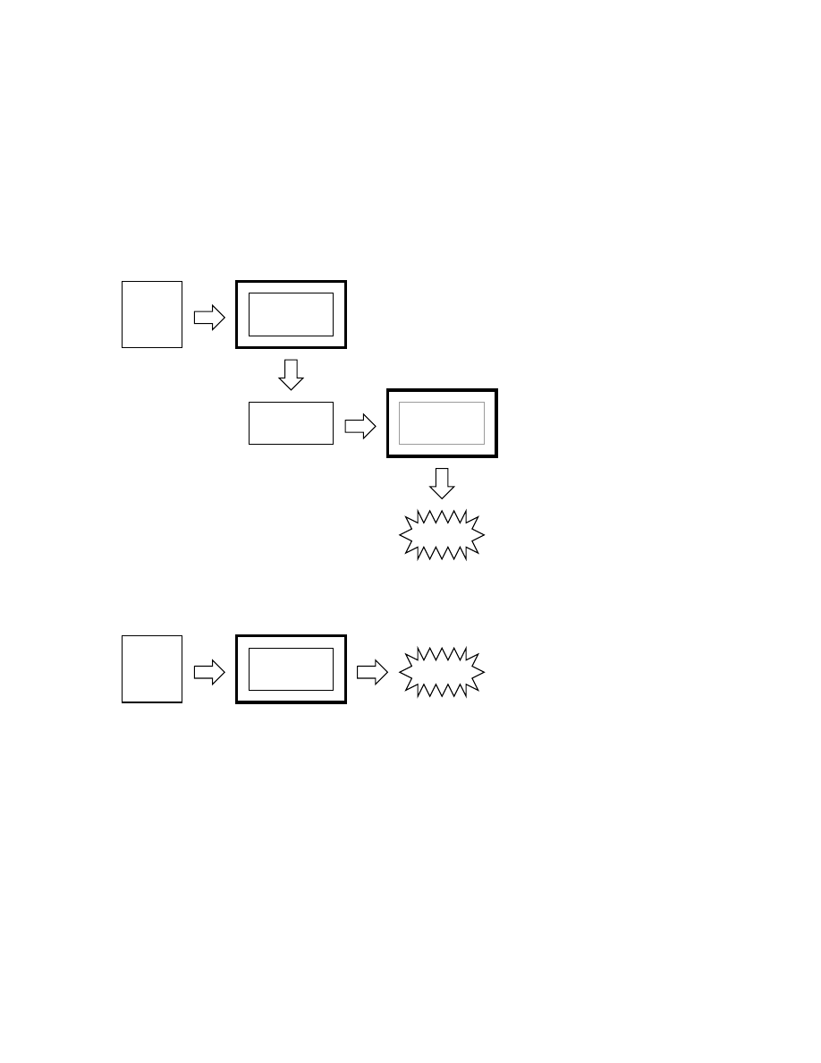
60
CHAPTER 7. USING THE SPICE CIRCUIT SIMULATION PROGRAM
In a compiled computer language, the program you wrote is translated all at once into the
computer’s own language by a special program called a compiler. After the program you’ve written
has been ”compiled,” the resulting executable file needs no further translation to be understood
directly by the computer. It can now be ”run” on a computer whether or not compiler software has
been installed on that computer:
Source
File
Computer
software
Output
Compiler
Computer
File
Executable
File
Executable
SPICE is an interpreted language. In order for a computer to be able to understand the SPICE
instructions you type, it must have the SPICE program (interpreter) installed:
Source
File
Computer
software
Output
"netlist"
SPICE
SPICE source files are commonly referred to as ”netlists,” although they are sometimes known as
”decks” with each line in the file being called a ”card.” Cute, don’t you think? Netlists are created
by a person like yourself typing instructions line-by-line using a word processor or text editor.
Text editors are much preferred over word processors for any type of computer programming, as
they produce pure ASCII text with no special embedded codes for text highlighting (like italic or
boldface fonts), which are uninterpretable by interpreter and compiler software.
As in general programming, the source file you create for SPICE must follow certain conventions
of programming. It is a computer language in itself, albeit a simple one. Having programmed in
BASIC and C/C++, and having some experience reading PASCAL and FORTRAN programs, it
is my opinion that the language of SPICE is much simpler than any of these. It is about the same
complexity as a markup language such as HTML, perhaps less so.
There is a cycle of steps to be followed in using SPICE to analyze a circuit. The cycle starts

7.3. FUNDAMENTALS OF SPICE PROGRAMMING
61
when you first invoke the text editing program and make your first draft of the netlist. The next
step is to run SPICE on that new netlist and see what the results are. If you are a novice user of
SPICE, your first attempts at creating a good netlist will be fraught with small errors of syntax.
Don’t worry – as every computer programmer knows, proficiency comes with lots of practice. If your
trial run produces error messages or results that are obviously incorrect, you need to re-invoke the
text editing program and modify the netlist. After modifying the netlist, you need to run SPICE
again and check the results. The sequence, then, looks something like this:
• Compose a new netlist with a text editing program. Save that netlist to a file with a name of
your choice.
• Run SPICE on that netlist and observe the results.
• If the results contain errors, start up the text editing program again and modify the netlist.
• Run SPICE again and observe the new results.
• If there are still errors in the output of SPICE, re-edit the netlist again with the text editing
program. Repeat this cycle of edit/run as many times as necessary until you are getting the
desired results.
• Once you’ve ”debugged” your netlist and are getting good results, run SPICE again, only this
time redirecting the output to a new file instead of just observing it on the computer screen.
• Start up a text editing program or a word processor program and open the SPICE output file
you just created. Modify that file to suit your formatting needs and either save those changes
to disk and/or print them out on paper.
To ”run” a SPICE ”program,” you need to type in a command at a terminal prompt interface,
such as that found in MS-DOS, UNIX, or the MS-Windows DOS prompt option:
spice < example.cir
The word ”spice” invokes the SPICE interpreting program (providing that the SPICE software
has been installed on the computer!), the ”<” symbol redirects the contents of the source file to the
SPICE interpreter, and example.cir is the name of the source file for this circuit example. The file
extension ”.cir” is not mandatory; I have seen ”.inp” (for ”input”) and just plain ”.txt” work
well, too. It will even work when the netlist file has no extension. SPICE doesn’t care what you
name it, so long as it has a name compatible with the filesystem of your computer (for old MS-DOS
machines, for example, the filename must be no more than 8 characters in length, with a 3 character
extension, and no spaces or other non-alphanumerical characters).
When this command is typed in, SPICE will read the contents of the example.cir file, analyze
the circuit specified by that file, and send a text report to the computer terminal’s standard output
(usually the screen, where you can see it scroll by). A typical SPICE output is several screens worth
of information, so you might want to look it over with a slight modification of the command:
spice < example.cir
| more
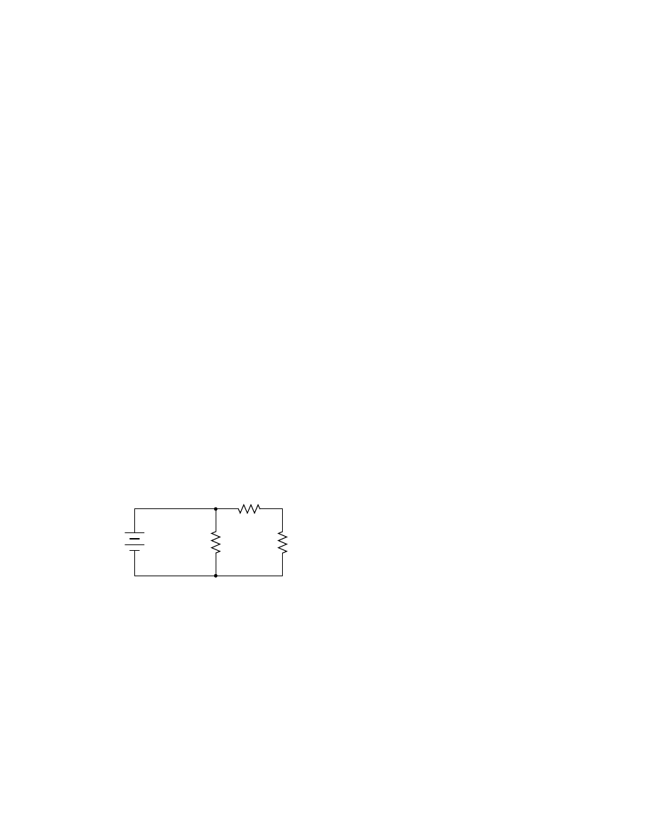
62
CHAPTER 7. USING THE SPICE CIRCUIT SIMULATION PROGRAM
This alternative ”pipes” the text output of SPICE to the ”more” utility, which allows only one
page to be displayed at a time. What this means (in English) is that the text output of SPICE
is halted after one screen-full, and waits until the user presses a keyboard key to display the next
screen-full of text. If you’re just testing your example circuit file and want to check for any errors,
this is a good way to do it.
spice < example.cir > example.txt
This second alternative (above) redirects the text output of SPICE to another file, called example.txt,
where it can be viewed or printed. This option corresponds to the last step in the development cycle
listed earlier. It is recommended by this author that you use this technique of ”redirection” to a
text file only after you’ve proven your example circuit netlist to work well, so that you don’t waste
time invoking a text editor just to see the output during the stages of ”debugging.”
Once you have a SPICE output stored in a .txt file, you can use a text editor or (better yet!) a
word processor to edit the output, deleting any unnecessary banners and messages, even specifying
alternative fonts to highlight the headings and/or data for a more polished appearance. Then, of
course, you can print the output to paper if you so desire. Being that the direct SPICE output is
plain ASCII text, such a file will be universally interpretable on any computer whether SPICE is
installed on it or not. Also, the plain text format ensures that the file will be very small compared
to the graphic screen-shot files generated by ”point-and-click” simulators.
The netlist file format required by SPICE is quite simple. A netlist file is nothing more than
a plain ASCII text file containing multiple lines of text, each line describing either a circuit com-
ponent or special SPICE command. Circuit architecture is specified by assigning numbers to each
component’s connection points in each line, connections between components designated by common
numbers. Examine the following example circuit diagram and its corresponding SPICE file. Please
bear in mind that the circuit diagram exists only to make the simulation easier for human beings to
understand. SPICE only understands netlists:
1
0
2
1
0
0
R
2
R
1
R
3
150
Ω
3.3 k
Ω
2.2 k
Ω
15 V
Example netlist
v1 1 0 dc 15
r1 1 0 2.2k
r2 1 2 3.3k
r3 2 0 150
.end
Each line of the source file shown above is explained here:

7.3. FUNDAMENTALS OF SPICE PROGRAMMING
63
• v1 represents the battery (voltage source 1), positive terminal numbered 1, negative terminal
numbered 0, with a DC voltage output of 15 volts.
• r1 represents resistor R
1
in the diagram, connected between points 1 and 0, with a value of
2.2 kΩ.
• r2 represents resistor R
2
in the diagram, connected between points 1 and 2, with a value of
3.3 kΩ.
• r3 represents resistor R
3
in the diagram, connected between points 2 and 0, with a value of
150 kΩ.
Electrically common points (or ”nodes”) in a SPICE circuit description share common numbers,
much in the same way that wires connecting common points in a large circuit typically share common
wire labels.
To simulate this circuit, the user would type those six lines of text on a text editor and save
them as a file with a unique name (such as example.cir). Once the netlist is composed and saved
to a file, the user then processes that file with one of the command-line statements shown earlier
(spice < example.cir), and will receive this text output on their computer’s screen:
1*******10/10/99 ******** spice 2g.6 3/15/83 ********07:32:42*****
0example netlist
0****
input listing
temperature =
27.000 deg c
v1 1 0 dc 15
r1 1 0 2.2k
r2 1 2 3.3k
r3 2 0 150
.end
*****10/10/99 *********
spice 2g.6
3/15/83 ******07:32:42******
0example netlist
0****
small signal bias solution
temperature =
27.000 deg c
node
voltage
node
voltage
(
1)
15.0000
(
2)
0.6522
voltage source currents
name
current
v1
-1.117E-02
total power dissipation
1.67E-01
watts
job concluded
0
total job time
0.02
1*******10/10/99 ********
spice 2g.6
3/15/83 ******07:32:42*****
0****
input listing
temperature =
27.000 deg c
SPICE begins by printing the time, date, and version used at the top of the output. It then lists
the input parameters (the lines of the source file), followed by a display of DC voltage readings from
each node (reference number) to ground (always reference number 0). This is followed by a list of
current readings through each voltage source (in this case there’s only one, v1). Finally, the total
power dissipation and computation time in seconds is printed.

64
CHAPTER 7. USING THE SPICE CIRCUIT SIMULATION PROGRAM
All output values provided by SPICE are displayed in scientific notation.
The SPICE output listing shown above is a little verbose for most peoples’ taste. For a final
presentation, it might be nice to trim all the unnecessary text and leave only what matters. Here is
a sample of that same output, redirected to a text file (spice < example.cir > example.txt),
then trimmed down judiciously with a text editor for final presentation and printed:
example netlist
v1 1 0 dc 15
r1 1 0 2.2k
r2 1 2 3.3k
r3 2 0 150
.end
node
voltage
node
voltage
(
1)
15.0000
(
2)
0.6522
voltage source currents
name
current
v1
-1.117E-02
total power dissipation
1.67E-01
watts
One of the very nice things about SPICE is that both input and output formats are plain-text,
which is the most universal and easy-to-edit electronic format around. Practically any computer
will be able to edit and display this format, even if the SPICE program itself is not resident on that
computer. If the user desires, he or she is free to use the advanced capabilities of word processing
programs to make the output look fancier. Comments can even be inserted between lines of the
output for further clarity to the reader.
7.4
The command-line interface
If you’ve used DOS or UNIX operating systems before in a command-line shell environment, you
may wonder why we have to use the ”<” symbol between the word ”spice” and the name of the
netlist file to be interpreted. Why not just enter the file name as the first argument to the command
”spice” as we do when we invoke the text editor? The answer is that SPICE has the option of an
interactive mode, whereby each line of the netlist can be interpreted as it is entered through the
computer’s Standard Input (stdin). If you simple type ”spice” at the prompt and press [Enter],
SPICE will begin to interpret anything you type in to it (live).
For most applications, it’s nice to save your netlist work in a separate file and then let SPICE
interpret that file when you’re ready. This is the way I encourage SPICE to be used, and so this is
the way it’s presented in this lesson. In order to use SPICE this way in a command-line environment,
we need to use the ”<” redirection symbol to direct the contents of your netlist file to Standard
Input (stdin), which SPICE can then process.

7.5. CIRCUIT COMPONENTS
65
7.5
Circuit components
Remember that this tutorial is not exhaustive by any means, and that all descriptions for elements
in the SPICE language are documented here in condensed form. SPICE is a very capable piece of
software with lots of options, and I’m only going to document a few of them.
All components in a SPICE source file are primarily identified by the first letter in each respective
line. Characters following the identifying letter are used to distinguish one component of a certain
type from another of the same type (r1, r2, r3, rload, rpullup, etc.), and need not follow any particular
naming convention, so long as no more than eight characters are used in both the component
identifying letter and the distinguishing name.
For example, suppose you were simulating a digital circuit with ”pullup” and ”pulldown” resis-
tors. The name rpullup would be valid because it is seven characters long. The name rpulldown,
however, is nine characters long. This may cause problems when SPICE interprets the netlist.
You can actually get away with component names in excess of eight total characters if there are
no other similarly-named components in the source file. SPICE only pays attention to the first eight
characters of the first field in each line, so rpulldown is actually interpreted as rpulldow with the
”n” at the end being ignored. Therefore, any other resistor having the first eight characters in its
first field will be seen by SPICE as the same resistor, defined twice, which will cause an error (i.e.
rpulldown1
and rpulldown2 would be interpreted as the same name, rpulldow).
It should also be noted that SPICE ignores character case, so r1 and R1 are interpreted by SPICE
as one and the same.
SPICE allows the use of metric prefixes in specifying component values, which is a very handy
feature. However, the prefix convention used by SPICE differs somewhat from standard metric
symbols, primarily due to the fact that netlists are restricted to standard ASCII characters (ruling
out Greek letters such as µ for the prefix ”micro”) and that SPICE is case-insensitive, so ”m”
(which is the standard symbol for ”milli”) and ”M” (which is the standard symbol for ”Mega”) are
interpreted identically. Here are a few examples of prefixes used in SPICE netlists:
r1 1 0 2t
(Resistor R
1
, 2t = 2 Tera-ohms = 2 TΩ)
r2 1 0 4g
(Resistor R
2
, 4g = 4 Giga-ohms = 4 GΩ)
r3 1 0 47meg
(Resistor R
3
, 47meg = 47 Mega-ohms = 47 MΩ)
r4 1 0 3.3k
(Resistor R
4
, 3.3k = 3.3 kilo-ohms = 3.3 kΩ)
r5 1 0 55m
(Resistor R
5
, 55m = 55 milli-ohms = 55 mΩ)
r6 1 0 10u
(Resistor R
6
, 10u = 10 micro-ohms 10 µΩ)
r7 1 0 30n
(Resistor R
7
, 30n = 30 nano-ohms = 30 nΩ)
r8 1 0 5p
(Resistor R
8
, 5p = 5 pico-ohms = 5 pΩ)
r9 1 0 250f
(Resistor R
9
, 250f = 250 femto-ohms = 250 fΩ)
Scientific notation is also allowed in specifying component values. For example:
r10 1 0 4.7e3
(Resistor R
10
, 4.7e3 = 4.7 x 10
3
ohms = 4.7 kilo-ohms = 4.7 kΩ)
r11 1 0 1e-12
(Resistor R
11
, 1e-12 = 1 x 10
−12
ohms = 1 pico-ohm = 1 pΩ)
The unit (ohms, volts, farads, henrys, etc.) is automatically determined by the type of component
being specified. SPICE ”knows” that all of the above examples are ”ohms” because they are all
resistors (r1, r2, r3, . . . ). If they were capacitors, the values would be interpreted as ”farads,” if
inductors, then ”henrys,” etc.

66
CHAPTER 7. USING THE SPICE CIRCUIT SIMULATION PROGRAM
7.5.1
Passive components
CAPACITORS:
General form:
c[name] [node1] [node2] [value] ic=[initial voltage]
Example 1:
c1 12 33 10u
Example 2:
c1 12 33 10u ic=3.5
Comments: The ”initial condition” (ic=) variable is the capacitor’s voltage in units of volts
at the start of DC analysis. It is an optional value, with the starting voltage assumed to be zero
if unspecified. Starting current values for capacitors are interpreted by SPICE only if the .tran
analysis option is invoked (with the ”uic” option).
INDUCTORS:
General form:
l[name] [node1] [node2] [value] ic=[initial current]
Example 1:
l1 12 33 133m
Example 2:
l1 12 33 133m ic=12.7m
Comments: The ”initial condition” (ic=) variable is the inductor’s current in units of amps at
the start of DC analysis. It is an optional value, with the starting current assumed to be zero if
unspecified. Starting current values for inductors are interpreted by SPICE only if the .tran analysis
option is invoked.
INDUCTOR COUPLING (transformers):
General form:
k[name] l[name] l[name] [coupling factor]
Example 1:
k1 l1 l2 0.999
Comments: SPICE will only allow coupling factor values between 0 and 1 (non-inclusive), with
0 representing no coupling and 1 representing perfect coupling. The order of specifying coupled
inductors (l1, l2 or l2, l1) is irrelevant.
RESISTORS:
General form:
r[name] [node1] [node2] [value]
Example:
rload 23 15 3.3k
Comments: In case you were wondering, there is no declaration of resistor power dissipation
rating in SPICE. All components are assumed to be indestructible. If only real life were this forgiving!
7.5.2
Active components
All semiconductor components must have their electrical characteristics described in a line starting
with the word ”.model”, which tells SPICE exactly how the device will behave. Whatever parame-
ters are not explicitly defined in the .model card will default to values pre-programmed in SPICE.
However, the .model card must be included, and at least specify the model name and device type
(d, npn, pnp, njf, pjf, nmos, or pmos).
DIODES:
General form:
d[name] [anode] [cathode] [model]
Example:
d1 1 2 mod1

7.5. CIRCUIT COMPONENTS
67
DIODE MODELS:
General form:
.model [modelname] d [parmtr1=x] [parmtr2=x] . . .
Example:
.model mod1 d
Example:
.model mod2 d vj=0.65 rs=1.3
Parameter definitions:
is
= saturation current in amps
rs
= junction resistance in ohms
n
= emission coefficient (unitless)
tt
= transit time in seconds
cjo
= zero-bias junction capacitance in farads
vj
= junction potential in volts
m
= grading coefficient (unitless)
eg
= activation energy in electron-volts
xti
= saturation-current temperature exponent (unitless)
kf
= flicker noise coefficient (unitless)
af
= flicker noise exponent (unitless)
fc
= forward-bias depletion capacitance coefficient (unitless)
bv
= reverse breakdown voltage in volts
ibv
= current at breakdown voltage in amps
Comments: The model name must begin with a letter, not a number. If you plan to specify
a model for a 1N4003 rectifying diode, for instance, you cannot use ”1n4003” for the model name.
An alternative might be ”m1n4003” instead.
TRANSISTORS (bipolar junction – BJT):
General form:
q[name] [collector] [base] [emitter] [model]
Example:
q1 2 3 0 mod1
BJT TRANSISTOR MODELS:
General form:
.model [modelname] [npn or pnp] [parmtr1=x] . . .
Example:
.model mod1 pnp
Example:
.model mod2 npn bf=75 is=1e-14
The model examples shown above are very nonspecific. To accurately model real-life transistors,
more parameters are necessary. Take these two examples, for the popular 2N2222 and 2N2907
transistors (the ”+”) characters represent line-continuation marks in SPICE, when you wish to
break a single line (card) into two or more separate lines on your text editor:
Example:
.model m2n2222 npn is=19f bf=150 vaf=100 ikf=.18
+
ise=50p ne=2.5 br=7.5 var=6.4 ikr=12m
+
isc=8.7p nc=1.2 rb=50 re=0.4 rc=0.4 cje=26p
+
tf=0.5n cjc=11p tr=7n xtb=1.5 kf=0.032f af=1
Example:
.model m2n2907 pnp is=1.1p bf=200 nf=1.2 vaf=50
+
ikf=0.1 ise=13p ne=1.9 br=6 rc=0.6 cje=23p
+
vje=0.85 mje=1.25 tf=0.5n cjc=19p vjc=0.5
+
mjc=0.2 tr=34n xtb=1.5
Parameter definitions:
is
= transport saturation current in amps
bf
= ideal maximum forward Beta (unitless)
nf
= forward current emission coefficient (unitless)

68
CHAPTER 7. USING THE SPICE CIRCUIT SIMULATION PROGRAM
vaf
= forward Early voltage in volts
ikf
= corner for forward Beta high-current rolloff in amps
ise
= B-E leakage saturation current in amps
ne
= B-E leakage emission coefficient (unitless)
br
= ideal maximum reverse Beta (unitless)
nr
= reverse current emission coefficient (unitless)
bar
= reverse Early voltage in volts
ikr
ikr = corner for reverse Beta high-current rolloff in amps
isc
isc = B-C leakage saturation current in amps
nc
= B-C leakage emission coefficient (unitless)
rb
= zero bias base resistance in ohms
irb
= current for base resistance halfway value in amps
rbm
= minimum base resistance at high currents in ohms
re
= emitter resistance in ohms
rc
= collector resistance in ohms
cje
= B-E zero-bias depletion capacitance in farads
vje
= B-E built-in potential in volts
mje
= B-E junction exponential factor (unitless)
tf
= ideal forward transit time (seconds)
xtf
= coefficient for bias dependence of transit time (unitless)
vtf
= B-C voltage dependence on transit time, in volts
itf
= high-current parameter effect on transit time, in amps
ptf
= excess phase at f=1/(transit time)(2)(pi) Hz, in degrees
cjc
= B-C zero-bias depletion capacitance in farads
vjc
= B-C built-in potential in volts
mjc
= B-C junction exponential factor (unitless)
xjcj
= B-C depletion capacitance fraction connected in base node (unitless)
tr
= ideal reverse transit time in seconds
cjs
= zero-bias collector-substrate capacitance in farads
vjs
= substrate junction built-in potential in volts
mjs
= substrate junction exponential factor (unitless)
xtb
= forward/reverse Beta temperature exponent
eg
= energy gap for temperature effect on transport saturation current in electron-volts
xti
= temperature exponent for effect on transport saturation current (unitless)
kf
= flicker noise coefficient (unitless)
af
= flicker noise exponent (unitless)
fc
= forward-bias depletion capacitance formula coefficient (unitless)
Comments: Just as with diodes, the model name given for a particular transistor type must
begin with a letter, not a number. That’s why the examples given above for the 2N2222 and 2N2907
types of BJTs are named ”m2n2222” and ”m2n2907” respectively.
As you can see, SPICE allows for very detailed specification of transistor properties. Many of the
properties listed above are well beyond the scope and interest of the beginning electronics student,
and aren’t even useful apart from knowing the equations SPICE uses to model BJT transistors. For
those interested in learning more about transistor modeling in SPICE, consult other books, such as
Andrei Vladimirescu’s The Spice Book (ISBN 0-471-60926-9).

7.5. CIRCUIT COMPONENTS
69
TRANSISTORS (junction field-effect – JFET):
General form:
j[name] [drain] [gate] [source] [model]
Example:
j1 2 3 0 mod1
JFET TRANSISTOR MODELS:
General form:
.model [modelname] [njf or pjf] [parmtr1=x] . . .
Example:
.model mod1 pjf
Example:
.model mod2 njf lambda=1e-5 pb=0.75
Parameter definitions:
vto
= threshold voltage in volts
beta
= transconductance parameter in amps/volts
2
lambda
= channel length modulation parameter in units of 1/volts
rd
= drain resistance in ohms
rs
= source resistance in ohms
cgs
= zero-bias G-S junction capacitance in farads
cgd
= zero-bias G-D junction capacitance in farads
pb
= gate junction potential in volts
is
= gate junction saturation current in amps
kf
= flicker noise coefficient (unitless)
af
= flicker noise exponent (unitless)
fc
= forward-bias depletion capacitance coefficient (unitless)
TRANSISTORS (insulated-gate field-effect – IGFET or MOSFET):
General form:
m[name] [drain] [gate] [source] [substrate] [model]
Example:
m1 2 3 0 0 mod1
MOSFET TRANSISTOR MODELS:
General form:
.model [modelname] [nmos or pmos] [parmtr1=x] . . .
Example:
.model mod1 pmos
Example:
.model mod2 nmos level=2 phi=0.65 rd=1.5
Example:
.model mod3 nmos vto=-1
(depletion)
Example:
.model mod4 nmos vto=1
(enhancement)
Example:
.model mod5 pmos vto=1
(depletion)
Example:
.model mod6 pmos vto=-1
(enhancement)
Comments: In order to distinguish between enhancement mode and depletion-mode (also
known as depletion-enhancement mode) transistors, the model parameter ”vto” (zero-bias threshold
voltage) must be specified. Its default value is zero, but a positive value (+1 volts, for example)
on a P-channel transistor or a negative value (-1 volts) on an N-channel transistor will specify that
transistor to be a depletion (otherwise known as depletion-enhancement) mode device. Conversely,
a negative value on a P-channel transistor or a positive value on an N-channel transistor will specify
that transistor to be an enhancement mode device.
Remember that enhancement mode transistors are normally-off devices, and must be turned
on by the application of gate voltage. Depletion-mode transistors are normally ”on,” but can be
”pinched off” as well as enhanced to greater levels of drain current by applied gate voltage, hence
the alternate designation of ”depletion-enhancement” MOSFETs. The ”vto” parameter specifies
the threshold gate voltage for MOSFET conduction.

70
CHAPTER 7. USING THE SPICE CIRCUIT SIMULATION PROGRAM
7.5.3
Sources
AC SINEWAVE VOLTAGE SOURCES (when using .ac card to specify frequency):
General form:
v[name] [+node] [-node] ac [voltage] [phase] sin
Example 1:
v1 1 0 ac 12 sin
Example 2:
v1 1 0 ac 12 240 sin
(12 V
6
240
o
)
Comments: This method of specifying AC voltage sources works well if you’re using multiple
sources at different phase angles from each other, but all at the same frequency. If you need to
specify sources at different frequencies in the same circuit, you must use the next method!
AC SINEWAVE VOLTAGE SOURCES (when NOT using .ac card to specify fre-
quency):
General form:
v[name] [+node] [-node] sin([offset] [voltage]
+
[freq] [delay] [damping factor])
Example 1:
v1 1 0 sin(0 12 60 0 0)
Parameter definitions:
offset
= DC bias voltage, offsetting the AC waveform by a specified voltage.
voltage
= peak, or crest, AC voltage value for the waveform.
freq
= frequency in Hertz.
delay
= time delay, or phase offset for the waveform, in seconds.
damping factor
= a figure used to create waveforms of decaying amplitude.
Comments: This method of specifying AC voltage sources works well if you’re using multi-
ple sources at different frequencies from each other. Representing phase shift is tricky, though,
necessitating the use of the delay factor.
DC VOLTAGE SOURCES (when using .dc card to specify voltage):
General form:
v[name] [+node] [-node] dc
Example 1:
v1 1 0 dc
Comments: If you wish to have SPICE output voltages not in reference to node 0, you must
use the .dc analysis option, and to use this option you must specify at least one of your DC sources
in this manner.
DC VOLTAGE SOURCES (when NOT using .dc card to specify voltage):
General form:
v[name] [+node] [-node] dc [voltage]
Example 1:
v1 1 0 dc 12
Comments: Nothing noteworthy here!
PULSE VOLTAGE SOURCES
General form:
v[name] [+node] [-node] pulse ([i] [p] [td] [tr]
+
[tf] [pw] [pd])
Parameter definitions:
i
= initial value
p
= pulse value
td
= delay time (all time parameters in units of seconds)
tr
= rise time
tf
= fall time

7.5. CIRCUIT COMPONENTS
71
pw
= pulse width
pd
= period
Example 1:
v1 1 0 pulse (-3 3 0 0 0 10m 20m)
Comments: Example 1 is a perfect square wave oscillating between -3 and +3 volts, with zero
rise and fall times, a 20 millisecond period, and a 50 percent duty cycle (+3 volts for 10 ms, then -3
volts for 10 ms).
AC SINEWAVE CURRENT SOURCES (when using .ac card to specify frequency):
General form:
i[name] [+node] [-node] ac [current] [phase] sin
Example 1:
i1 1 0 ac 3 sin
(3 amps)
Example 2:
i1 1 0 ac 1m 240 sin
(1 mA
6
240
o
)
Comments: The same comments apply here (and in the next example) as for AC voltage
sources.
AC SINEWAVE CURRENT SOURCES (when NOT using .ac card to specify fre-
quency):
General form:
i[name] [+node] [-node] sin([offset]
+
[current] [freq] 0 0)
Example 1:
i1 1 0 sin(0 1.5 60 0 0)
DC CURRENT SOURCES (when using .dc card to specify current):
General form:
i[name] [+node] [-node] dc
Example 1:
i1 1 0 dc
DC CURRENT SOURCES (when NOT using .dc card to specify current):
General form:
i[name] [+node] [-node] dc [current]
Example 1:
i1 1 0 dc 12
Comments: Even though the books all say that the first node given for the DC current source
is the positive node, that’s not what I’ve found to be in practice. In actuality, a DC current source
in SPICE pushes current in the same direction as a voltage source (battery) would with its negative
node specified first.
PULSE CURRENT SOURCES
General form:
i[name] [+node] [-node] pulse ([i] [p] [td] [tr]
+
[tf] [pw] [pd])
Parameter definitions:
i
= initial value
p
= pulse value
td
= delay time
tr
= rise time
tf
= fall time
pw
= pulse width
pd
= period
Example 1:
i1 1 0 pulse (-3m 3m 0 0 0 17m 34m)

72
CHAPTER 7. USING THE SPICE CIRCUIT SIMULATION PROGRAM
Comments: Example 1 is a perfect square wave oscillating between -3 mA and +3 mA, with
zero rise and fall times, a 34 millisecond period, and a 50 percent duty cycle (+3 mA for 17 ms,
then -3 mA for 17 ms).
VOLTAGE SOURCES (dependent):
General form:
e[name] [out+node] [out-node] [in+node] [in-node]
+
[gain]
Example 1:
e1 2 0 1 2 999k
Comments: Dependent voltage sources are great to use for simulating operational amplifiers.
Example 1 shows how such a source would be configured for use as a voltage follower, inverting
input connected to output (node 2) for negative feedback, and the noninverting input coming in on
node 1. The gain has been set to an arbitrarily high value of 999,000. One word of caution, though:
SPICE does not recognize the input of a dependent source as being a load, so a voltage source tied
only to the input of an independent voltage source will be interpreted as ”open.” See op-amp circuit
examples for more details on this.
CURRENT SOURCES (dependent):
7.6
Analysis options
AC ANALYSIS:
General form:
.ac [curve] [points] [start] [final]
Example 1:
.ac lin 1 1000 1000
Comments: The [curve] field can be ”lin” (linear), ”dec” (decade), or ”oct” (octave), specifying
the (non)linearity of the frequency sweep. ¡points¿ specifies how many points within the frequency
sweep to perform analyses at (for decade sweep, the number of points per decade; for octave, the
number of points per octave). The [start] and [final] fields specify the starting and ending frequencies
of the sweep, respectively. One final note: the ”start” value cannot be zero!
DC ANALYSIS:
General form:
.dc [source] [start] [final] [increment]
Example 1:
.dc vin 1.5 15 0.5
Comments: The .dc card is necessary if you want to print or plot any voltage between two
nonzero nodes. Otherwise, the default ”small-signal” analysis only prints out the voltage between
each nonzero node and node zero.
TRANSIENT ANALYSIS:
General form:
.tran [increment] [stop time] [start time]
+
[comp interval]
Example 1:
.tran 1m 50m uic
Example 2:
.tran .5m 32m 0 .01m
Comments: Example 1 has an increment time of 1 millisecond and a stop time of 50 milliseconds
(when only two parameters are specified, they are increment time and stop time, respectively).
Example 2 has an increment time of 0.5 milliseconds, a stop time of 32 milliseconds, a start time of
0 milliseconds (no delay on start), and a computation interval of 0.01 milliseconds.

7.6. ANALYSIS OPTIONS
73
Default value for start time is zero. Transient analysis always beings at time zero, but storage
of data only takes place between start time and stop time. Data output interval is increment time,
or (stop time - start time)/50, which ever is smallest. However, the computing interval variable can
be used to force a computational interval smaller than either. For large total interval counts, the
itl5
variable in the .options card may be set to a higher number. The ”uic” option tells SPICE
to ”use initial conditions.”
PLOT OUTPUT:
General form:
.plot [type] [output1] [output2] . . . [output n]
Example 1:
.plot dc v(1,2) i(v2)
Example 2:
.plot ac v(3,4) vp(3,4) i(v1) ip(v1)
Example 3:
.plot tran v(4,5) i(v2)
Comments: SPICE can’t handle more than eight data point requests on a single .plot or
card. If requesting more than eight data points, use multiple cards!
Also, here’s a major caveat when using SPICE version 3: if you’re performing AC analysis and
you ask SPICE to plot an AC voltage as in example #2, the v(3,4) command will only output
the real component of a rectangular-form complex number! SPICE version 2 outputs the polar
magnitude of a complex number: a much more meaningful quantity if only a single quantity is asked
for. To coerce SPICE3 to give you polar magnitude, you will have to re-write the .print or .plot
argument as such: vm(3,4).
PRINT OUTPUT:
General form:
.print [type] [output1] [output2] . . . [output n]
Example 1:
.print dc v(1,2) i(v2)
Example 2:
.print ac v(2,4) i(vinput) vp(2,3)
Example 3:
.print tran v(4,5) i(v2)
Comments: SPICE can’t handle more than eight data point requests on a single .plot or
card. If requesting more than eight data points, use multiple cards!
FOURIER ANALYSIS:
General form:
.four [freq] [output1] [output2] . . . [output n]
Example 1:
.four 60 v(1,2)
Comments: The .four card relies on the .tran card being present somewhere in the deck,
with the proper time periods for analysis of adequate cycles. Also, SPICE may ”crash” if a .plot
analysis isn’t done along with the .four analysis, even if all .tran parameters are technically correct.
Finally, the .four analysis option only works when the frequency of the AC source is specified in
that source’s card line, and not in an .ac analysis option line.
It helps to include a computation interval variable in the .tran card for better analysis precision.
A Fourier analysis of the voltage or current specified is performed up to the 9th harmonic, with the
[freq] specification being the fundamental, or starting frequency of the analysis spectrum.
MISCELLANEOUS:
General form:
.options [option1] [option2]
Example 1:
.options limpts=500
Example 2:
.options itl5=0
Example 3:
.options method=gear

74
CHAPTER 7. USING THE SPICE CIRCUIT SIMULATION PROGRAM
Example 4:
.options list
Example 5:
.options nopage
Example 6:
.options numdgt=6
Comments: There are lots of options that can be specified using this card. Perhaps the one
most needed by beginning users of SPICE is the ”limpts” setting. When running a simulation
that requires more than 201 points to be printed or plotted, this calculation point limit must be
increased or else SPICE will terminate analysis. The example given above (limpts=500) tells SPICE
to allocate enough memory to handle at least 500 calculation points in whatever type of analysis is
specified (DC, AC, or transient).
In example 2, we see an iteration variable (itl5) being set to a value of 0. There are actually six
different iteration variables available for user manipulation. They control the iteration cycle limits
for solution of nonlinear equations. The variable itl5 sets the maximum number of iterations for
a transient analysis. Similar to the limpts variable, itl5 usually needs to be set when a small
computation interval has been specified on a .tran card. Setting itl5 to a value of 0 turns off the
limit entirely, allowing the computer infinite iteration cycles (infinite time) to compute the analysis.
Warning: this may result in long simulation times!
Example 3 with ”method=gear” sets the numerical integration method used by SPICE. The
default is ”trapezoid” rather than ”gear,” trapezoid being a simple geometric approximation of area
under a curve found by slicing up the curve into trapezoids to approximate the shape. The ”gear”
method is based on second-order or better polynomial equations and is named after C.W. Gear
(Numerical Integration of Stiff Ordinary Equations, Report 221, Department of Computer Science,
University of Illinois, Urbana). The Gear method of integration is more demanding of the computer
(computationally ”expensive”) and will sometimes give slightly different results from the trapezoid
method.
The ”list” option shown in example 4 gives a verbose summary of all circuit components and
their respective values in the final output.
By default, SPICE will insert ASCII page-break control codes in the output to separate different
sections of the analysis. Specifying the ”nopage” option (example 5) will prevent such pagination.
The ”numdgt” option shown in example 6 specifies the number of significant digits output when
using one of the ”.print” data output options. SPICE defaults at a precision of 4 significant digits.
WIDTH CONTROL:
General form:
.width in=[columns] out=[columns]
Example 1:
.width out=80
Comments: The .width card can be used to control the width of text output lines upon
analysis. This is especially handy when plotting graphs with the .plot card. The default value is
120, which can cause problems on 80-character terminal displays unless set to 80 with this command.
7.7
Quirks
”Garbage in, garbage out.”
Anonymous
SPICE is a very reliable piece of software, but it does have its little quirks that take some getting
used to. By ”quirk” I mean a demand placed upon the user to write the source file in a particular

7.7. QUIRKS
75
way in order for it to work without giving error messages. I do not mean any kind of fault with
SPICE which would produce erroneous or misleading results: that would be more properly referred
to as a ”bug.” Speaking of bugs, SPICE has a few of them as well.
Some (or all) of these quirks may be unique to SPICE version 2g6, which is the only version I’ve
used extensively. They may have been fixed in later versions.
7.7.1
A good beginning
SPICE demands that the source file begin with something other than the first ”card” in the circuit
description ”deck.” This first character in the source file can be a linefeed, title line, or a comment:
there just has to be something there before the first component-specifying line of the file. If not,
SPICE will refuse to do an analysis at all, claiming that there is a serious error (such as improper
node connections) in the ”deck.”
7.7.2
A good ending
SPICE demands that the .end line at the end of the source file not be terminated with a linefeed
or carriage return character. In other words, when you finish typing ”.end” you should not hit the
[Enter] key on your keyboard. The cursor on your text editor should stop immediately to the right
of the ”d” after the ”.end” and go no further. Failure to heed this quirk will result in a ”missing
.end card ” error message at the end of the analysis output. The actual circuit analysis is not affected
by this error, so I normally ignore the message. However, if you’re looking to receive a ”perfect”
output, you must pay heed to this idiosyncrasy.
7.7.3
Must have a node 0
You are given much freedom in numbering circuit nodes, but you must have a node 0 somewhere in
your netlist in order for SPICE to work. Node 0 is the default node for circuit ground, and it is the
point of reference for all voltages specified at single node locations.
When simple DC analysis is performed by SPICE, the output will contain a listing of voltages
at all non-zero nodes in the circuit. The point of reference (ground) for all these voltage readings is
node 0. For example:
node
voltage
node
voltage
(
1)
15.0000
(
2)
0.6522
In this analysis, there is a DC voltage of 15 volts between node 1 and ground (node 0), and a
DC voltage of 0.6522 volts between node 2 and ground (node 0). In both these cases, the voltage
polarity is negative at node 0 with reference to the other node (in other words, both nodes 1 and 2
are positive with respect to node 0).
7.7.4
Avoid open circuits
SPICE cannot handle open circuits of any kind. If your netlist specifies a circuit with an open
voltage source, for example, SPICE will refuse to perform an analysis. A prime example of this type
of error is found when ”connecting” a voltage source to the input of a voltage-dependent source
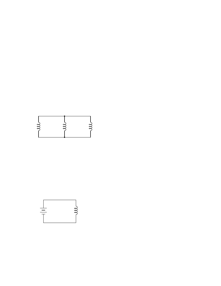
76
CHAPTER 7. USING THE SPICE CIRCUIT SIMULATION PROGRAM
(used to simulate an operational amplifier). SPICE needs to see a complete path for current, so I
usually tie a high-value resistor (call it rbogus!) across the voltage source to act as a minimal load.
7.7.5
Avoid certain component loops
SPICE cannot handle certain uninterrupted loops of components in a circuit, namely voltage sources
and inductors. The following loops will cause SPICE to abort analysis:
2
2
2
4
4
4
L
1
L
2
L
3
10 mH
50 mH
25 mH
Parallel inductors
netlist
l1 2 4 10m
l2 2 4 50m
l3 2 4 25m
1
1
0
0
Voltage source / inductor loop
V
1
12 V
L
1
150 mH
netlist
v1 1 0 dc 12
l1 1 0 150m

7.7. QUIRKS
77
5
6
7
Series capacitors
C
1
33
µ
F
C
2
47
µ
F
netlist
c1 5 6 33u
c2 6 7 47u
The reason SPICE can’t handle these conditions stems from the way it performs DC analysis:
by treating all inductors as shorts and all capacitors as opens. Since short-circuits (0 Ω) and open
circuits (infinite resistance) either contain or generate mathematical infinitudes, a computer simply
cannot deal with them, and so SPICE will discontinue analysis if any of these conditions occur.
In order to make these component configurations acceptable to SPICE, you must insert resistors
of appropriate values into the appropriate places, eliminating the respective short-circuits and open-
circuits. If a series resistor is required, choose a very low resistance value. Conversely, if a parallel
resistor is required, choose a very high resistance value. For example:
To fix the parallel inductor problem, insert a very low-value resistor in series with each offending
inductor.
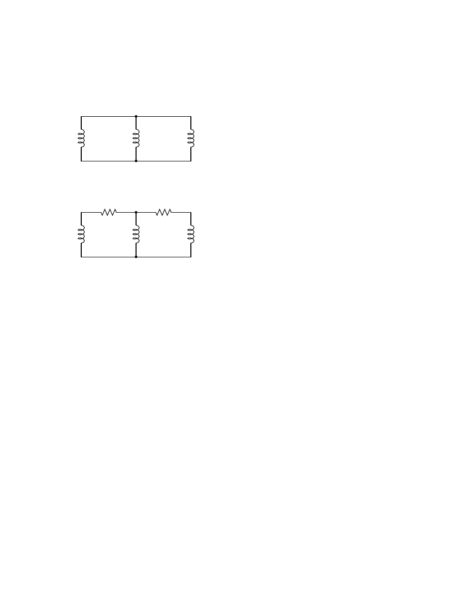
78
CHAPTER 7. USING THE SPICE CIRCUIT SIMULATION PROGRAM
2
2
2
4
4
4
4
4
4
R
bogus1
R
bogus2
2
3
5
Original circuit
"Fixed" circuit
L
1
10 mH
L
2
50 mH
L
3
25 mH
L
1
10 mH
L
2
50 mH
L
3
25 mH
original netlist
l1 2 4 10m
l2 2 4 50m
l3 2 4 25m
fixed netlist
rbogus1 2 3 1e-12
rbogus2 2 5 1e-12
l1 3 4 10m
l2 2 4 50m
l3 5 4 25m
The extremely low-resistance resistors R
bogus1
and R
bogus2
(each one with a mere 1 pico-ohm
of resistance) ”break up” the direct parallel connections that existed between L
1
, L
2
, and L
3
. It is
important to choose very low resistances here so that circuit operation is not substantially impacted
by the ”fix.”
To fix the voltage source / inductor loop, insert a very low-value resistor in series with the two
components.
7.7. QUIRKS
79
1
1
0
0
1
0
0
R
bogus
2
Original circuit
"Fixed" circuit
V
1
12 V
L
1
150 mH
V
1
12 V
L
1
150 mH
original netlist
v1 1 0 dc 12
l1 1 0 150m
fixed netlist
v1 1 0 dc 12
l1 2 0 150m
rbogus 1 2 1e-12
As in the previous example with parallel inductors, it is important to make the correction resistor
(R
bogus
) very low in resistance, so as to not substantially impact circuit operation.
To fix the series capacitor circuit, one of the capacitors must have a resistor shunting across it.
SPICE requires a DC current path to each capacitor for analysis.
80
CHAPTER 7. USING THE SPICE CIRCUIT SIMULATION PROGRAM
5
6
7
5
6
7
7
6
R
bogus
Original circuit
"Fixed" circuit
C
1
33
µ
F
C
2
47
µ
F
C
1
33
µ
F
C
2
47
µ
F
original netlist
c1 5 6 33u
c2 6 7 47u
fixed netlist
c1 5 6 33u
c2 6 7 47u
rbogus 6 7 9e12
The R
bogus
value of 9 Tera-ohms provides a DC current path to C
1
(and around C
2
) without
substantially impacting the circuit’s operation.
7.7.6
Current measurement
Although printing or plotting of voltage is quite easy in SPICE, the output of current values is a bit
more difficult. Voltage measurements are specified by declaring the appropriate circuit nodes. For
example, if we desire to know the voltage across a capacitor whose leads connect between nodes 4
and 7, we might make out .print statement look like this:
4
7
C
1
22
µ
F
c1 4 7 22u
.print ac v(4,7)
However, if we wanted to have SPICE measure the current through that capacitor, it wouldn’t be
quite so easy. Currents in SPICE must be specified in relation to a voltage source, not any arbitrary
component. For example:
7.7. QUIRKS
81
4
7
V
input
6
C
1
22
µ
F
I
c1 4 7 22u
vinput 6 4 ac 1 sin
.print ac i(vinput)
This .print card instructs SPICE to print the current through voltage source V
input
, which
happens to be the same as the current through our capacitor between nodes 4 and 7. But what if
there is no such voltage source in our circuit to reference for current measurement? One solution is
to insert a shunt resistor into the circuit and measure voltage across it. In this case, I have chosen
a shunt resistance value of 1 Ω to produce 1 volt per amp of current through C
1
:
4
7
6
R
shunt
C
1
22
µ
F
I
1
Ω
c1 4 7 22u
rshunt 6 4 1
.print ac v(6,4)
However, the insertion of an extra resistance into our circuit large enough to drop a meaningful
voltage for the intended range of current might adversely affect things. A better solution for SPICE
is this, although one would never seek such a current measurement solution in real life:
4
7
6
V
bogus
C
1
22
µ
F
I
0 V
c1 4 7 22u
vbogus 6 4 dc 0
.print ac i(vbogus)
Inserting a ”bogus” DC voltage source of zero volts doesn’t affect circuit operation at all, yet
it provides a convenient place for SPICE to take a current measurement. Interestingly enough, it
doesn’t matter that V
bogus
is a DC source when we’re looking to measure AC current! The fact that
SPICE will output an AC current reading is determined by the ”ac” specification in the .print
card and nothing more.
It should also be noted that the way SPICE assigns a polarity to current measurements is a bit
odd. Take the following circuit as an example:
82
CHAPTER 7. USING THE SPICE CIRCUIT SIMULATION PROGRAM
10 V
1
2
0
0
V
1
R
1
R
2
5 k
Ω
5 k
Ω
example
v1 1 0
r1 1 2 5k
r2 2 0 5k
.dc v1 10 10 1
.print dc i(v1)
.end
With 10 volts total voltage and 10 kΩ total resistance, you might expect SPICE to tell you
there’s going to be 1 mA (1e-03) of current through voltage source V
1
, but in actuality SPICE will
output a figure of negative 1 mA (-1e-03)! SPICE regards current out of the negative end of a DC
voltage source (the normal direction) to be a negative value of current rather than a positive value
of current. There are times I’ll throw in a ”bogus” voltage source in a DC circuit like this simply to
get SPICE to output a positive current value:
10 V
1
2
0
V
1
R
1
R
2
5 k
Ω
5 k
Ω
V
bogus
0 V
3
example
v1 1 0
r1 1 2 5k
r2 2 3 5k
vbogus 3 0 dc 0
.dc v1 10 10 1
.print dc i(vbogus)
.end
Notice how V
bogus
is positioned so that the circuit current will enter its positive side (node 3)
and exit its negative side (node 0). This orientation will ensure a positive output figure for circuit
current.
7.8. EXAMPLE CIRCUITS AND NETLISTS
83
7.7.7
Fourier analysis
When performing a Fourier (frequency-domain) analysis on a waveform, I have found it necessary to
either print or plot the waveform using the .print or .plot cards, respectively. If you don’t print
or plot it, SPICE will pause for a moment during analysis and then abort the job after outputting
the ”initial transient solution.”
Also, when analyzing a square wave produced by the ”pulse” source function, you must give
the waveform some finite rise and fall time, or else the Fourier analysis results will be incorrect.
For some reason, a perfect square wave with zero rise/fall time produces significant levels of even
harmonics according to SPICE’s Fourier analysis option, which is not true for real square waves.
7.8
Example circuits and netlists
The following circuits are pre-tested netlists for SPICE 2g6, complete with short descriptions when
necessary. Feel free to ”copy” and ”paste” any of the netlists to your own SPICE source file for
analysis and/or modification. My goal here is twofold: to give practical examples of SPICE netlist
design to further understanding of SPICE netlist syntax, and to show how simple and compact
SPICE netlists can be in analyzing simple circuits.
All output listings for these examples have been ”trimmed” of extraneous information, giving
you the most succinct presentation of the SPICE output as possible. I do this primarily to save
space on this document. Typical SPICE outputs contain lots of headers and summary information
not necessarily germane to the task at hand. So don’t be surprised when you run a simulation on
your own and find that the output doesn’t exactly look like what I have shown here!
7.8.1
Multiple-source DC resistor network, part 1
1
2
3
0
0
0
V
1
24 V
R
1
R
2
R
3
V
2
10 k
Ω
8.1 k
Ω
4.7 k
Ω
15 V
Without a .dc card and a .print or .plot card, the output for this netlist will only display
voltages for nodes 1, 2, and 3 (with reference to node 0, of course).
Netlist:
Multiple dc sources
v1 1 0 dc 24
v2 3 0 dc 15
r1 1 2 10k
r2 2 3 8.1k
r3 2 0 4.7k
84
CHAPTER 7. USING THE SPICE CIRCUIT SIMULATION PROGRAM
.end
Output:
node
voltage
node
voltage
node
voltage
(
1)
24.0000
(
2)
9.7470
(
3)
15.0000
voltage source currents
name
current
v1
-1.425E-03
v2
-6.485E-04
total power dissipation
4.39E-02
watts
7.8.2
Multiple-source DC resistor network, part 2
1
2
3
0
0
0
V
1
24 V
R
1
R
2
R
3
V
2
10 k
Ω
8.1 k
Ω
4.7 k
Ω
15 V
By adding a .dc analysis card and specifying source V
1
from 24 volts to 24 volts in 1 step (in
other words, 24 volts steady), we can use the .print card analysis to print out voltages between any
two points we desire. Oddly enough, when the .dc analysis option is invoked, the default voltage
printouts for each node (to ground) disappears, so we end up having to explicitly specify them in
the .print card to see them at all.
Netlist:
Multiple dc sources
v1 1 0
v2 3 0 15
r1 1 2 10k
r2 2 3 8.1k
r3 2 0 4.7k
.dc v1 24 24 1
.print dc v(1) v(2) v(3) v(1,2) v(2,3)
.end
Output:
v1
v(1)
v(2)
v(3)
v(1,2)
v(2,3)
2.400E+01
2.400E+01
9.747E+00
1.500E+01
1.425E+01
-5.253E+00
7.8. EXAMPLE CIRCUITS AND NETLISTS
85
7.8.3
RC time-constant circuit
1
1
1
2
2
0
V
1
10 V
C
1
47
µ
F
C
2
22
µ
F
R
1
3.3 k
Ω
For DC analysis, the initial conditions of any reactive component (C or L) must be specified
(voltage for capacitors, current for inductors). This is provided by the last data field of each capacitor
card (ic=0). To perform a DC analysis, the .tran (”transient”) analysis option must be specified,
with the first data field specifying time increment in seconds, the second specifying total analysis
timespan in seconds, and the ”uic” telling it to ”use initial conditions” when analyzing.
Netlist:
RC time delay circuit
v1 1 0 dc 10
c1 1 2 47u ic=0
c2 1 2 22u ic=0
r1 2 0 3.3k
.tran .05 1 uic
.print tran v(1,2)
.end
Output:
time
v(1,2)
0.000E+00
7.701E-06
5.000E-02
1.967E+00
1.000E-01
3.551E+00
1.500E-01
4.824E+00
2.000E-01
5.844E+00
2.500E-01
6.664E+00
3.000E-01
7.322E+00
3.500E-01
7.851E+00
4.000E-01
8.274E+00
4.500E-01
8.615E+00
5.000E-01
8.888E+00
5.500E-01
9.107E+00
6.000E-01
9.283E+00
6.500E-01
9.425E+00
7.000E-01
9.538E+00
7.500E-01
9.629E+00
8.000E-01
9.702E+00

86
CHAPTER 7. USING THE SPICE CIRCUIT SIMULATION PROGRAM
8.500E-01
9.761E+00
9.000E-01
9.808E+00
9.500E-01
9.846E+00
1.000E+00
9.877E+00
7.8.4
Plotting and analyzing a simple AC sinewave voltage
R
load
15 V
60 Hz
1
1
0
0
10 k
Ω
V
1
This exercise does show the proper setup for plotting instantaneous values of a sine-wave voltage
source with the .plot function (as a transient analysis). Not surprisingly, the Fourier analysis in this
deck also requires the .tran (transient) analysis option to be specified over a suitable time range.
The time range in this particular deck allows for a Fourier analysis with rather poor accuracy. The
more cycles of the fundamental frequency that the transient analysis is performed over, the more
precise the Fourier analysis will be. This is not a quirk of SPICE, but rather a basic principle of
waveforms.
Netlist:
v1 1 0 sin(0 15 60 0 0)
rload 1 0 10k
* change tran card to the following for better Fourier precision
* .tran 1m 30m .01m
and include .options card:
* .options itl5=30000
.tran 1m 30m
.plot tran v(1)
.four 60 v(1)
.end
Output:
time
v(1)
-2.000E+01
-1.000E+01
0.000E+00
1.000E+01
- - - - - - - - - - - - - - - - - - - - - - - - - - - - - - - - - -
0.000E+00
0.000E+00 .
.
*
.
.
1.000E-03
5.487E+00 .
.
.
*
.
.
2.000E-03
1.025E+01 .
.
.
*
.
3.000E-03
1.350E+01 .
.
.
.
*
.
4.000E-03
1.488E+01 .
.
.
.
*.
5.000E-03
1.425E+01 .
.
.
.
* .
6.000E-03
1.150E+01 .
.
.
. *
.
7.000E-03
7.184E+00 .
.
.
*
.
.
8.000E-03
1.879E+00 .
.
.
*
.
.
9.000E-03 -3.714E+00 .
.
*
.
.
.

7.8. EXAMPLE CIRCUITS AND NETLISTS
87
1.000E-02 -8.762E+00 .
. *
.
.
.
1.100E-02 -1.265E+01 .
*
.
.
.
.
1.200E-02 -1.466E+01 .
*
.
.
.
.
1.300E-02 -1.465E+01 .
*
.
.
.
.
1.400E-02 -1.265E+01 .
*
.
.
.
.
1.500E-02 -8.769E+00 .
. *
.
.
.
1.600E-02 -3.709E+00 .
.
*
.
.
.
1.700E-02
1.876E+00 .
.
.
*
.
.
1.800E-02
7.191E+00 .
.
.
*
.
.
1.900E-02
1.149E+01 .
.
.
. *
.
2.000E-02
1.425E+01 .
.
.
.
* .
2.100E-02
1.489E+01 .
.
.
.
*.
2.200E-02
1.349E+01 .
.
.
.
*
.
2.300E-02
1.026E+01 .
.
.
*
.
2.400E-02
5.491E+00 .
.
.
*
.
.
2.500E-02
1.553E-03 .
.
*
.
.
2.600E-02 -5.514E+00 .
.
*
.
.
.
2.700E-02 -1.022E+01 .
*
.
.
.
2.800E-02 -1.349E+01 .
*
.
.
.
.
2.900E-02 -1.495E+01 .
*
.
.
.
.
3.000E-02 -1.427E+01 .
*
.
.
.
.
- - - - - - - - - - - - - - - - - - - - - - - - - - - - - - - - - -
fourier components of transient response v(1)
dc component =
-1.885E-03
harmonic
frequency
fourier
normalized
phase
normalized
no
(hz)
component
component
(deg)
phase (deg)
1
6.000E+01
1.494E+01
1.000000
-71.998
0.000
2
1.200E+02
1.886E-02
0.001262
-50.162
21.836
3
1.800E+02
1.346E-03
0.000090
102.674
174.671
4
2.400E+02
1.799E-02
0.001204
-10.866
61.132
5
3.000E+02
3.604E-03
0.000241
160.923
232.921
6
3.600E+02
5.642E-03
0.000378
-176.247
-104.250
7
4.200E+02
2.095E-03
0.000140
122.661
194.658
8
4.800E+02
4.574E-03
0.000306
-143.754
-71.757
9
5.400E+02
4.896E-03
0.000328
-129.418
-57.420
total harmonic distortion =
0.186350
percent
88
CHAPTER 7. USING THE SPICE CIRCUIT SIMULATION PROGRAM
7.8.5
Simple AC resistor-capacitor circuit
12 V
60 Hz
1
2
0
0
R
1
30
Ω
C
1
100
µ
F
V
1
The .ac card specifies the points of ac analysis from 60Hz to 60Hz, at a single point. This card,
of course, is a bit more useful for multi-frequency analysis, where a range of frequencies can be
analyzed in steps. The .print card outputs the AC voltage between nodes 1 and 2, and the AC
voltage between node 2 and ground.
Netlist:
Demo of a simple AC circuit
v1 1 0 ac 12 sin
r1 1 2 30
c1 2 0 100u
.ac lin 1 60 60
.print ac v(1,2) v(2)
.end
Output:
freq
v(1,2)
v(2)
6.000E+01
8.990E+00
7.949E+00
7.8.6
Low-pass filter
1
0
2
24 V
24 V
R
load
3
4
0
0
V
1
V
2
L
1
L
2
100 mH
250 mH
C
1
100
µ
F
1 k
Ω

7.8. EXAMPLE CIRCUITS AND NETLISTS
89
This low-pass filter blocks AC and passes DC to the R
load
resistor. Typical of a filter used to
suppress ripple from a rectifier circuit, it actually has a resonant frequency, technically making it a
band-pass filter. However, it works well anyway to pass DC and block the high-frequency harmonics
generated by the AC-to-DC rectification process. Its performance is measured with an AC source
sweeping from 500 Hz to 15 kHz. If desired, the .print card can be substituted or supplemented
with a .plot card to show AC voltage at node 4 graphically.
Netlist:
Lowpass filter
v1 2 1 ac 24 sin
v2 1 0 dc 24
rload 4 0 1k
l1 2 3 100m
l2 3 4 250m
c1 3 0 100u
.ac lin 30 500 15k
.print ac v(4)
.plot ac v(4)
.end
freq
v(4)
5.000E+02
1.935E-01
1.000E+03
3.275E-02
1.500E+03
1.057E-02
2.000E+03
4.614E-03
2.500E+03
2.402E-03
3.000E+03
1.403E-03
3.500E+03
8.884E-04
4.000E+03
5.973E-04
4.500E+03
4.206E-04
5.000E+03
3.072E-04
5.500E+03
2.311E-04
6.000E+03
1.782E-04
6.500E+03
1.403E-04
7.000E+03
1.124E-04
7.500E+03
9.141E-05
8.000E+03
7.536E-05
8.500E+03
6.285E-05
9.000E+03
5.296E-05
9.500E+03
4.504E-05
1.000E+04
3.863E-05
1.050E+04
3.337E-05
1.100E+04
2.903E-05
1.150E+04
2.541E-05
1.200E+04
2.237E-05
1.250E+04
1.979E-05

90
CHAPTER 7. USING THE SPICE CIRCUIT SIMULATION PROGRAM
1.300E+04
1.760E-05
1.350E+04
1.571E-05
1.400E+04
1.409E-05
1.450E+04
1.268E-05
1.500E+04
1.146E-05
freq
v(4)
1.000E-06
1.000E-04
1.000E-02
1.000E+00
- - - - - - - - - - - - - - - - - - - - - - - - - - - - - - - - - -
5.000E+02
1.935E-01 .
.
.
*
.
1.000E+03
3.275E-02 .
.
.
*
.
1.500E+03
1.057E-02 .
.
*
.
2.000E+03
4.614E-03 .
.
* .
.
2.500E+03
2.402E-03 .
.
*
.
.
3.000E+03
1.403E-03 .
.
*
.
.
3.500E+03
8.884E-04 .
.
*
.
.
4.000E+03
5.973E-04 .
.
*
.
.
4.500E+03
4.206E-04 .
.
*
.
.
5.000E+03
3.072E-04 .
.
*
.
.
5.500E+03
2.311E-04 .
.
*
.
.
6.000E+03
1.782E-04 .
. *
.
.
6.500E+03
1.403E-04 .
.*
.
.
7.000E+03
1.124E-04 .
*
.
.
7.500E+03
9.141E-05 .
*
.
.
8.000E+03
7.536E-05 .
*.
.
.
8.500E+03
6.285E-05 .
*.
.
.
9.000E+03
5.296E-05 .
* .
.
.
9.500E+03
4.504E-05 .
* .
.
.
1.000E+04
3.863E-05 .
*
.
.
.
1.050E+04
3.337E-05 .
*
.
.
.
1.100E+04
2.903E-05 .
*
.
.
.
1.150E+04
2.541E-05 .
*
.
.
.
1.200E+04
2.237E-05 .
*
.
.
.
1.250E+04
1.979E-05 .
*
.
.
.
1.300E+04
1.760E-05 .
*
.
.
.
1.350E+04
1.571E-05 .
*
.
.
.
1.400E+04
1.409E-05 .
*
.
.
.
1.450E+04
1.268E-05 .
*
.
.
.
1.500E+04
1.146E-05 .
*
.
.
.
- - - - - - - - - - - - - - - - - - - - - - - - - - - - - - - - - -
7.8. EXAMPLE CIRCUITS AND NETLISTS
91
7.8.7
Multiple-source AC network
0
2
3
0
0
1
55 V
30 Hz
+
-
43 V
30 Hz
+
-
V
1
0
o
25
o
V
2
L
1
L
2
450 mH
150 mH
C
1
330
µ
F
One of the idiosyncrasies of SPICE is its inability to handle any loop in a circuit exclusively
composed of series voltage sources and inductors. Therefore, the ”loop” of V
1
-L
1
-L
2
-V
2
-V
1
is
unacceptable. To get around this, I had to insert a low -resistance resistor somewhere in that loop to
break it up. Thus, we have R
bogus
between 3 and 4 (with 1 pico-ohm of resistance), and V
2
between
4 and 0. The circuit above is the original design, while the circuit below has R
bogus
inserted to avoid
the SPICE error.
0
2
3
0
0
1
55 V
30 Hz
+
-
43 V
30 Hz
+
-
V
1
0
o
25
o
V
2
L
1
L
2
450 mH
150 mH
C
1
330
µ
F
4
R
bogus
1 p
Ω
Netlist:
Multiple ac source
v1 1 0 ac 55 0 sin
v2 4 0 ac 43 25 sin
l1 1 2 450m
c1 2 0 330u
l2 2 3 150m
92
CHAPTER 7. USING THE SPICE CIRCUIT SIMULATION PROGRAM
rbogus 3 4 1e-12
.ac lin 1 30 30
.print ac v(2)
.end
Output:
freq
v(2)
3.000E+01
1.413E+02
7.8.8
AC phase shift demonstration
R
shunt1
R
shunt2
1
1
1
0
0
0
1
Ω
1
Ω
6.3 k
Ω
R
1
L
1
2
3
1 H
The currents through each leg are indicated by the voltage drops across each respective shunt
resistor (1 amp = 1 volt through 1 Ω), output by the v(1,2) and v(1,3) terms of the .print card.
The phase of the currents through each leg are indicated by the phase of the voltage drops across
each respective shunt resistor, output by the vp(1,2) and vp(1,3) terms in the .print card.
Netlist:
phase shift
v1 1 0 ac 4 sin
rshunt1 1 2 1
rshunt2 1 3 1
l1 2 0 1
r1 3 0 6.3k
.ac lin 1 1000 1000
.print ac v(1,2) v(1,3) vp(1,2) vp(1,3)
.end
Output:
freq
v(1,2)
v(1,3)
vp(1,2)
vp(1,3)
1.000E+03
6.366E-04
6.349E-04
-9.000E+01
0.000E+00
7.8. EXAMPLE CIRCUITS AND NETLISTS
93
7.8.9
Transformer circuit
1
0
2
3
L
1
L
2
L
3
R
1
R
2
100 H
1 H
25 H
R
bogus1
R
bogus2
V
1
4
5
0
0
R
bogus0
SPICE understands transformers as a set of mutually coupled inductors. Thus, to simulate a
transformer in SPICE, you must specify the primary and secondary windings as separate inductors,
then instruct SPICE to link them together with a ”k” card specifying the coupling constant. For
ideal transformer simulation, the coupling constant would be unity (1). However, SPICE can’t
handle this value, so we use something like 0.999 as the coupling factor.
Note that all winding inductor pairs must be coupled with their own k cards in order for the
simulation to work properly. For a two-winding transformer, a single k card will suffice. For a
three-winding transformer, three k cards must be specified (to link L
1
with L
2
, L
2
with L
3
, and L
1
with L
3
).
The L
1
/L
2
inductance ratio of 100:1 provides a 10:1 step-down voltage transformation ratio.
With 120 volts in we should see 12 volts out of the L
2
winding. The L
1
/L
3
inductance ratio of
100:25 (4:1) provides a 2:1 step-down voltage transformation ratio, which should give us 60 volts
out of the L
3
winding with 120 volts in.
Netlist:
transformer
v1 1 0 ac 120 sin
rbogus0 1 6 1e-3
l1 6 0 100
l2 2 4 1
l3 3 5 25
k1 l1 l2 0.999
k2 l2 l3 0.999
k3 l1 l3 0.999
r1 2 4 1000
r2 3 5 1000
rbogus1 5 0 1e10
rbogus2 4 0 1e10
.ac lin 1 60 60
.print ac v(1,0) v(2,0) v(3,0)
.end
94
CHAPTER 7. USING THE SPICE CIRCUIT SIMULATION PROGRAM
Output:
freq
v(1)
v(2)
v(3)
6.000E+01
1.200E+02
1.199E+01
5.993E+01
In this example, R
bogus0
is a very low-value resistor, serving to break up the source/inductor
loop of V
1
/L
1
. R
bogus1
and R
bogus2
are very high-value resistors necessary to provide DC paths to
ground on each of the isolated circuits. Note as well that one side of the primary circuit is directly
grounded. Without these ground references, SPICE will produce errors!
7.8.10
Full-wave bridge rectifier
15 V
60 Hz
+
-
R
load
1
0
3
2
1
0
V
1
D
1
D
3
D
2
D
4
10 k
Ω
Diodes, like all semiconductor components in SPICE, must be modeled so that SPICE knows
all the nitty-gritty details of how they’re supposed to work. Fortunately, SPICE comes with a few
generic models, and the diode is the most basic. Notice the .model card which simply specifies ”d”
as the generic diode model for mod1. Again, since we’re plotting the waveforms here, we need to
specify all parameters of the AC source in a single card and print/plot all values using the .tran
option.
Netlist:
fullwave bridge rectifier
v1 1 0 sin(0 15 60 0 0)
rload 1 0 10k
d1 1 2 mod1
d2 0 2 mod1
d3 3 1 mod1
d4 3 0 mod1
.model mod1 d
.tran .5m 25m
.plot tran v(1,0) v(2,3)
.end
Output:
legend:
*: v(1)
+: v(2,3)
time
v(1)
(*)--------- -2.000E+01
-1.000E+01
0.000E+00
1.000E+01
2.000E+01

7.8. EXAMPLE CIRCUITS AND NETLISTS
95
(+)--------- -5.000E+00
0.000E+00
5.000E+00
1.000E+01
1.500E+01
- - - - - - - - - - - - - - - - - - - - - - - - - - - - - - - - - -
0.000E+00
0.000E+00 .
+
*
.
.
5.000E-04
2.806E+00 .
.
+
.
*
.
.
1.000E-03
5.483E+00 .
.
+
*
.
.
1.500E-03
7.929E+00 .
.
.
+
*
.
.
2.000E-03
1.013E+01 .
.
.
+*
.
2.500E-03
1.198E+01 .
.
.
.
* +
.
3.000E-03
1.338E+01 .
.
.
.
*
+
.
3.500E-03
1.435E+01 .
.
.
.
*
+.
4.000E-03
1.476E+01 .
.
.
.
*
+
4.500E-03
1.470E+01 .
.
.
.
*
+
5.000E-03
1.406E+01 .
.
.
.
*
+ .
5.500E-03
1.299E+01 .
.
.
.
*
+
.
6.000E-03
1.139E+01 .
.
.
. *+
.
6.500E-03
9.455E+00 .
.
.
+ *.
.
7.000E-03
7.113E+00 .
.
.
+
*
.
.
7.500E-03
4.591E+00 .
.
+.
*
.
.
8.000E-03
1.841E+00 .
.
+
. *
.
.
8.500E-03 -9.177E-01 .
.
+
*.
.
.
9.000E-03 -3.689E+00 .
.
*+
.
.
.
9.500E-03 -6.380E+00 .
.
*
. +
.
.
1.000E-02 -8.784E+00 .
. *
.
+
.
.
1.050E-02 -1.075E+01 .
*.
.
.+
.
1.100E-02 -1.255E+01 .
*
.
.
.
+
.
1.150E-02 -1.372E+01 .
*
.
.
.
+
.
1.200E-02 -1.460E+01 . *
.
.
.
+
1.250E-02 -1.476E+01 .*
.
.
.
+
1.300E-02 -1.460E+01 . *
.
.
.
+
1.350E-02 -1.373E+01 .
*
.
.
.
+
.
1.400E-02 -1.254E+01 .
*
.
.
.
+
.
1.450E-02 -1.077E+01 .
*.
.
.+
.
1.500E-02 -8.726E+00 .
. *
.
+
.
.
1.550E-02 -6.293E+00 .
.
*
. +
.
.
1.600E-02 -3.684E+00 .
.
x
.
.
.
1.650E-02 -9.361E-01 .
.
+
*.
.
.
1.700E-02
1.875E+00 .
.
+
. *
.
.
1.750E-02
4.552E+00 .
.
+.
*
.
.
1.800E-02
7.170E+00 .
.
.
+
*
.
.
1.850E-02
9.401E+00 .
.
.
+ *.
.
1.900E-02
1.146E+01 .
.
.
. *+
.
1.950E-02
1.293E+01 .
.
.
.
*
+
.
2.000E-02
1.414E+01 .
.
.
.
*
+.
2.050E-02
1.464E+01 .
.
.
.
*
+
2.100E-02
1.483E+01 .
.
.
.
*
+
2.150E-02
1.430E+01 .
.
.
.
*
+.
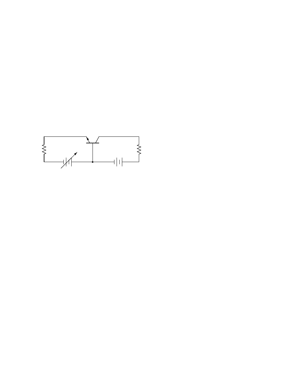
96
CHAPTER 7. USING THE SPICE CIRCUIT SIMULATION PROGRAM
2.200E-02
1.344E+01 .
.
.
.
*
+
.
2.250E-02
1.195E+01 .
.
.
.
*+
.
2.300E-02
1.016E+01 .
.
.
+*
.
2.350E-02
7.917E+00 .
.
.
+
*
.
.
2.400E-02
5.460E+00 .
.
+
*
.
.
2.450E-02
2.809E+00 .
.
+
.
*
.
.
2.500E-02 -8.297E-04 .
+
*
.
.
- - - - - - - - - - - - - - - - - - - - - - - - - - - - - - - - - -
7.8.11
Common-base BJT transistor amplifier
V
in
V
supply
24 V
0 to 5 V
R
e
R
c
0
1
2
3
4
Q
1
β
= 50
800
Ω
100
Ω
This analysis sweeps the input voltage (Vin) from 0 to 5 volts in 0.1 volt increments, then prints
out the voltage between the collector and emitter leads of the transistor v(2,3). The transistor (Q1)
is an NPN with a forward Beta of 50.
Netlist:
Common-base BJT amplifier
vsupply 1 0 dc 24
vin 0 4 dc
rc 1 2 800
re 3 4 100
q1 2 0 3 mod1
.model mod1 npn bf=50
.dc vin 0 5 0.1
.print dc v(2,3)
.plot dc v(2,3)
.end
Output:
vin
v(2,3)
0.000E+00
2.400E+01
1.000E-01
2.410E+01
2.000E-01
2.420E+01
3.000E-01
2.430E+01
4.000E-01
2.440E+01
5.000E-01
2.450E+01

7.8. EXAMPLE CIRCUITS AND NETLISTS
97
6.000E-01
2.460E+01
7.000E-01
2.466E+01
8.000E-01
2.439E+01
9.000E-01
2.383E+01
1.000E+00
2.317E+01
1.100E+00
2.246E+01
1.200E+00
2.174E+01
1.300E+00
2.101E+01
1.400E+00
2.026E+01
1.500E+00
1.951E+01
1.600E+00
1.876E+01
1.700E+00
1.800E+01
1.800E+00
1.724E+01
1.900E+00
1.648E+01
2.000E+00
1.572E+01
2.100E+00
1.495E+01
2.200E+00
1.418E+01
2.300E+00
1.342E+01
2.400E+00
1.265E+01
2.500E+00
1.188E+01
2.600E+00
1.110E+01
2.700E+00
1.033E+01
2.800E+00
9.560E+00
2.900E+00
8.787E+00
3.000E+00
8.014E+00
3.100E+00
7.240E+00
3.200E+00
6.465E+00
3.300E+00
5.691E+00
3.400E+00
4.915E+00
3.500E+00
4.140E+00
3.600E+00
3.364E+00
3.700E+00
2.588E+00
3.800E+00
1.811E+00
3.900E+00
1.034E+00
4.000E+00
2.587E-01
4.100E+00
9.744E-02
4.200E+00
7.815E-02
4.300E+00
6.806E-02
4.400E+00
6.141E-02
4.500E+00
5.657E-02
4.600E+00
5.281E-02
4.700E+00
4.981E-02
4.800E+00
4.734E-02
4.900E+00
4.525E-02
5.000E+00
4.346E-02

98
CHAPTER 7. USING THE SPICE CIRCUIT SIMULATION PROGRAM
vin
v(2,3) 0.000E+00
1.000E+01
2.000E+01
3.000E+01
- - - - - - - - - - - - - - - - - - - - - - - - - - - - - - - - - -
0.000E+00
2.400E+01 .
.
.
*
.
1.000E-01
2.410E+01 .
.
.
*
.
2.000E-01
2.420E+01 .
.
.
*
.
3.000E-01
2.430E+01 .
.
.
*
.
4.000E-01
2.440E+01 .
.
.
*
.
5.000E-01
2.450E+01 .
.
.
*
.
6.000E-01
2.460E+01 .
.
.
*
.
7.000E-01
2.466E+01 .
.
.
*
.
8.000E-01
2.439E+01 .
.
.
*
.
9.000E-01
2.383E+01 .
.
.
*
.
1.000E+00
2.317E+01 .
.
.
*
.
1.100E+00
2.246E+01 .
.
.
*
.
1.200E+00
2.174E+01 .
.
. *
.
1.300E+00
2.101E+01 .
.
.*
.
1.400E+00
2.026E+01 .
.
*
.
1.500E+00
1.951E+01 .
.
*.
.
1.600E+00
1.876E+01 .
.
* .
.
1.700E+00
1.800E+01 .
.
*
.
.
1.800E+00
1.724E+01 .
.
*
.
.
1.900E+00
1.648E+01 .
.
*
.
.
2.000E+00
1.572E+01 .
.
*
.
.
2.100E+00
1.495E+01 .
.
*
.
.
2.200E+00
1.418E+01 .
.
*
.
.
2.300E+00
1.342E+01 .
.
*
.
.
2.400E+00
1.265E+01 .
.
*
.
.
2.500E+00
1.188E+01 .
.
*
.
.
2.600E+00
1.110E+01 .
. *
.
.
2.700E+00
1.033E+01 .
*
.
.
2.800E+00
9.560E+00 .
*.
.
.
2.900E+00
8.787E+00 .
* .
.
.
3.000E+00
8.014E+00 .
*
.
.
.
3.100E+00
7.240E+00 .
*
.
.
.
3.200E+00
6.465E+00 .
*
.
.
.
3.300E+00
5.691E+00 .
*
.
.
.
3.400E+00
4.915E+00 .
*
.
.
.
3.500E+00
4.140E+00 .
*
.
.
.
3.600E+00
3.364E+00 .
*
.
.
.
3.700E+00
2.588E+00 .
*
.
.
.
3.800E+00
1.811E+00 .
*
.
.
.
3.900E+00
1.034E+00 .*
.
.
.
4.000E+00
2.587E-01 *
.
.
.
4.100E+00
9.744E-02 *
.
.
.
4.200E+00
7.815E-02 *
.
.
.
4.300E+00
6.806E-02 *
.
.
.
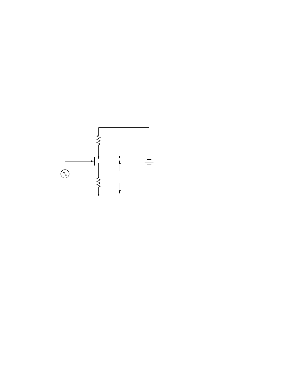
7.8. EXAMPLE CIRCUITS AND NETLISTS
99
4.400E+00
6.141E-02 *
.
.
.
4.500E+00
5.657E-02 *
.
.
.
4.600E+00
5.281E-02 *
.
.
.
4.700E+00
4.981E-02 *
.
.
.
4.800E+00
4.734E-02 *
.
.
.
4.900E+00
4.525E-02 *
.
.
.
5.000E+00
4.346E-02 *
.
.
.
- - - - - - - - - - - - - - - - - - - - - - - - - - - - - - - - - -
7.8.12
Common-source JFET amplifier with self-bias
V
DD
V
in
1 V
60 Hz
R
drain
R
source
1
0
0
0
2
3
4
3
V
out
10 k
Ω
20 V
1 k
Ω
J
1
Netlist:
common source jfet amplifier
vin 1 0 sin(0 1 60 0 0)
vdd 3 0 dc 20
rdrain 3 2 10k
rsource 4 0 1k
j1 2 1 4 mod1
.model mod1 njf
.tran 1m 30m
.plot tran v(2,0) v(1,0)
.end
Output:
legend:
*: v(2)
+: v(1)
time
v(2)
(*)---------
1.400E+01
1.600E+01
1.800E+01
2.000E+01 2.200E+01
(+)--------- -1.000E+00
-5.000E-01
0.000E+00
5.000E-01 1.000E+00
- - - - - - - - - - - - - - - - - - - - - - - - - - - - - - - - - -
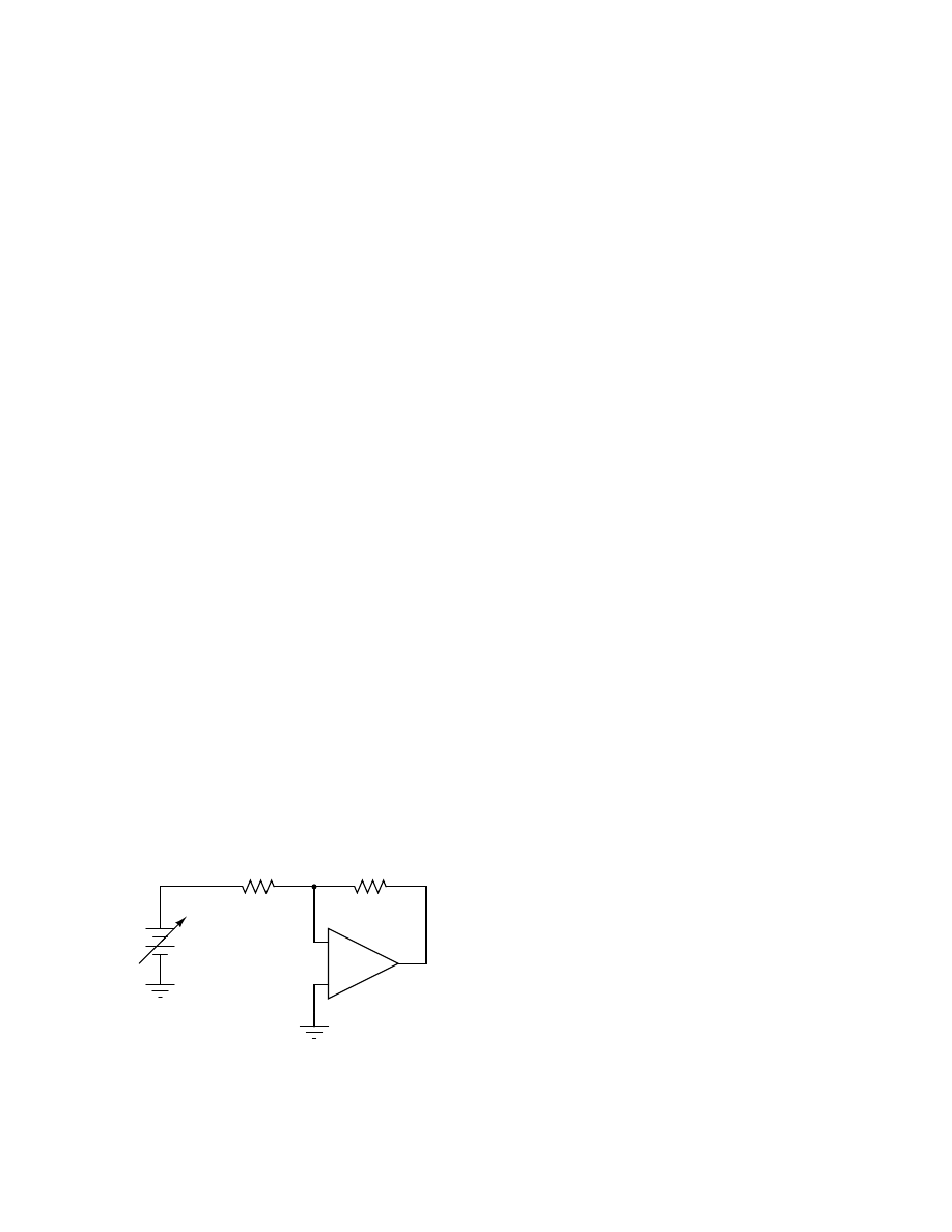
100
CHAPTER 7. USING THE SPICE CIRCUIT SIMULATION PROGRAM
0.000E+00
1.708E+01 .
.
*
+
.
.
1.000E-03
1.609E+01 .
.*
.
+ .
.
2.000E-03
1.516E+01 .
*
.
.
.
+
.
3.000E-03
1.448E+01 .
*
.
.
.
+
.
4.000E-03
1.419E+01 .*
.
.
.
+
5.000E-03
1.432E+01 . *
.
.
.
+.
6.000E-03
1.490E+01 .
*
.
.
.
+
.
7.000E-03
1.577E+01 .
* .
.
+.
.
8.000E-03
1.676E+01 .
.
*
.
+
.
.
9.000E-03
1.768E+01 .
.
+
*.
.
.
1.000E-02
1.841E+01 .
+ .
. *
.
.
1.100E-02
1.890E+01 .
+
.
.
*
.
.
1.200E-02
1.912E+01 .+
.
.
*
.
.
1.300E-02
1.912E+01 .+
.
.
*
.
.
1.400E-02
1.890E+01 .
+
.
.
*
.
.
1.500E-02
1.842E+01 .
+ .
. *
.
.
1.600E-02
1.768E+01 .
.
+
*.
.
.
1.700E-02
1.676E+01 .
.
*
.
+
.
.
1.800E-02
1.577E+01 .
* .
.
+.
.
1.900E-02
1.491E+01 .
*
.
.
.
+
.
2.000E-02
1.432E+01 . *
.
.
.
+.
2.100E-02
1.419E+01 .*
.
.
.
+
2.200E-02
1.449E+01 .
*
.
.
.
+
.
2.300E-02
1.516E+01 .
*
.
.
.
+
.
2.400E-02
1.609E+01 .
.*
.
+ .
.
2.500E-02
1.708E+01 .
.
*
+
.
.
2.600E-02
1.796E+01 .
. +
*
.
.
2.700E-02
1.861E+01 .
+
.
.
*
.
.
2.800E-02
1.900E+01 .
+
.
.
*
.
.
2.900E-02
1.916E+01 +
.
.
*
.
.
3.000E-02
1.908E+01 .+
.
.
*
.
.
- - - - - - - - - - - - - - - - - - - - - - - - - - - - - - - - - -
7.8.13
Inverting op-amp circuit
−
+
0 to 3.5
1
0
0
2
1
3
3
(e)
V
V
1
R
2
R
1
1.18 k
Ω
3.29 k
Ω

7.8. EXAMPLE CIRCUITS AND NETLISTS
101
To simulate an ideal operational amplifier in SPICE, we use a voltage-dependent voltage source
as a differential amplifier with extremely high gain. The ”e” card sets up the dependent voltage
source with four nodes, 3 and 0 for voltage output, and 1 and 0 for voltage input. No power supply
is needed for the dependent voltage source, unlike a real operational amplifier. The voltage gain is
set at 999,000 in this case. The input voltage source (V
1
) sweeps from 0 to 3.5 volts in 0.05 volt
steps.
Netlist:
Inverting opamp
v1 2 0 dc
e 3 0 0 1 999k
r1 3 1 3.29k
r2 1 2 1.18k
.dc v1 0 3.5 0.05
.print dc v(3,0)
.end
Output:
v1
v(3)
0.000E+00
0.000E+00
5.000E-02
-1.394E-01
1.000E-01
-2.788E-01
1.500E-01
-4.182E-01
2.000E-01
-5.576E-01
2.500E-01
-6.970E-01
3.000E-01
-8.364E-01
3.500E-01
-9.758E-01
4.000E-01
-1.115E+00
4.500E-01
-1.255E+00
5.000E-01
-1.394E+00
5.500E-01
-1.533E+00
6.000E-01
-1.673E+00
6.500E-01
-1.812E+00
7.000E-01
-1.952E+00
7.500E-01
-2.091E+00
8.000E-01
-2.231E+00
8.500E-01
-2.370E+00
9.000E-01
-2.509E+00
9.500E-01
-2.649E+00
1.000E+00
-2.788E+00
1.050E+00
-2.928E+00
1.100E+00
-3.067E+00
1.150E+00
-3.206E+00
1.200E+00
-3.346E+00
1.250E+00
-3.485E+00
1.300E+00
-3.625E+00

102
CHAPTER 7. USING THE SPICE CIRCUIT SIMULATION PROGRAM
1.350E+00
-3.764E+00
1.400E+00
-3.903E+00
1.450E+00
-4.043E+00
1.500E+00
-4.182E+00
1.550E+00
-4.322E+00
1.600E+00
-4.461E+00
1.650E+00
-4.600E+00
1.700E+00
-4.740E+00
1.750E+00
-4.879E+00
1.800E+00
-5.019E+00
1.850E+00
-5.158E+00
1.900E+00
-5.297E+00
1.950E+00
-5.437E+00
2.000E+00
-5.576E+00
2.050E+00
-5.716E+00
2.100E+00
-5.855E+00
2.150E+00
-5.994E+00
2.200E+00
-6.134E+00
2.250E+00
-6.273E+00
2.300E+00
-6.413E+00
2.350E+00
-6.552E+00
2.400E+00
-6.692E+00
2.450E+00
-6.831E+00
2.500E+00
-6.970E+00
2.550E+00
-7.110E+00
2.600E+00
-7.249E+00
2.650E+00
-7.389E+00
2.700E+00
-7.528E+00
2.750E+00
-7.667E+00
2.800E+00
-7.807E+00
2.850E+00
-7.946E+00
2.900E+00
-8.086E+00
2.950E+00
-8.225E+00
3.000E+00
-8.364E+00
3.050E+00
-8.504E+00
3.100E+00
-8.643E+00
3.150E+00
-8.783E+00
3.200E+00
-8.922E+00
3.250E+00
-9.061E+00
3.300E+00
-9.201E+00
3.350E+00
-9.340E+00
3.400E+00
-9.480E+00
3.450E+00
-9.619E+00
3.500E+00
-9.758E+00
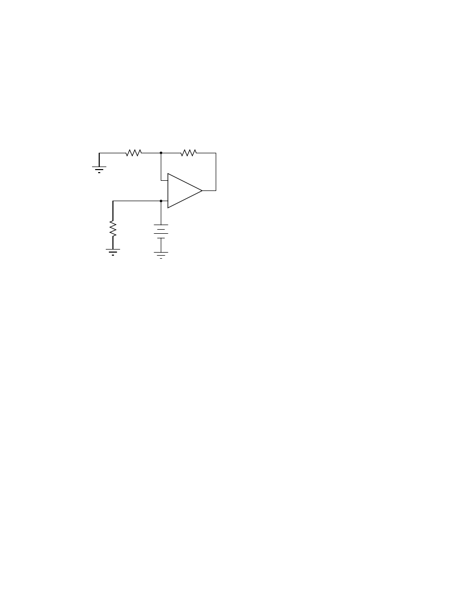
7.8. EXAMPLE CIRCUITS AND NETLISTS
103
7.8.14
Noninverting op-amp circuit
−
+
1
0
1
3
3
(e)
2
0
R
bogus
2
0
10 k
Ω
V
1
5 V
10 k
Ω
20 k
Ω
R
2
R
1
Another example of a SPICE quirk: since the dependent voltage source ”e” isn’t considered a
load to voltage source V
1
, SPICE interprets V
1
to be open-circuited and will refuse to analyze it.
The fix is to connect R
bogus
in parallel with V
1
to act as a DC load. Being directly connected across
V
1
, the resistance of R
bogus
is not crucial to the operation of the circuit, so 10 kΩ will work fine.
I decided not to sweep the V
1
input voltage at all in this circuit for the sake of keeping the netlist
and output listing simple.
Netlist:
noninverting opamp
v1 2 0 dc 5
rbogus 2 0 10k
e 3 0 2 1 999k
r1 3 1 20k
r2 1 0 10k
.end
Output:
node
voltage
node
voltage
node
voltage
(
1)
5.0000
(
2)
5.0000
(
3)
15.0000
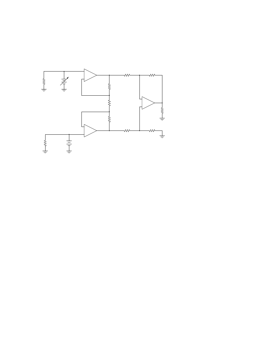
104
CHAPTER 7. USING THE SPICE CIRCUIT SIMULATION PROGRAM
7.8.15
Instrumentation amplifier
−
+
−
+
−
+
R
gain
R
load
(e1)
(e2)
(e3)
3
2
5
6
1
2
4
5
7
7
8
8
9
9
0
0
0
0
0
0
1
4
R
bogus1
R
bogus2
V
1
0 to 10 V
V
2
5 V
R
1
R
2
R
3
R
4
R
5
R
6
10 k
Ω
10 k
Ω
10 k
Ω
10 k
Ω
10 k
Ω
10 k
Ω
10 k
Ω
10 k
Ω
Note the very high-resistance R
bogus1
and R
bogus2
resistors in the netlist (not shown in schematic
for brevity) across each input voltage source, to keep SPICE from thinking V
1
and V
2
were open-
circuited, just like the other op-amp circuit examples.
Netlist:
Instrumentation amplifier
v1 1 0
rbogus1 1 0 9e12
v2 4 0 dc 5
rbogus2 4 0 9e12
e1 3 0 1 2 999k
e2 6 0 4 5 999k
e3 9 0 8 7 999k
rload 9 0 10k
r1 2 3 10k
rgain 2 5 10k
r2 5 6 10k
r3 3 7 10k
r4 7 9 10k
r5 6 8 10k
r6 8 0 10k
.dc v1 0 10 1
.print dc v(9) v(3,6)
.end
Output:
v1
v(9)
v(3,6)
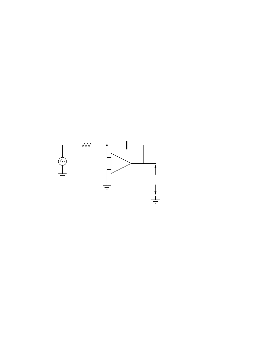
7.8. EXAMPLE CIRCUITS AND NETLISTS
105
0.000E+00
1.500E+01
-1.500E+01
1.000E+00
1.200E+01
-1.200E+01
2.000E+00
9.000E+00
-9.000E+00
3.000E+00
6.000E+00
-6.000E+00
4.000E+00
3.000E+00
-3.000E+00
5.000E+00
9.955E-11
-9.956E-11
6.000E+00
-3.000E+00
3.000E+00
7.000E+00
-6.000E+00
6.000E+00
8.000E+00
-9.000E+00
9.000E+00
9.000E+00
-1.200E+01
1.200E+01
1.000E+01
-1.500E+01
1.500E+01
7.8.16
Op-amp integrator with sinewave input
−
+
1
2
3
0
0
0
2
(e)
15 V
60 Hz
V
out
0
V
in
R
1
C
1
10 k
Ω
100
µ
F
Netlist:
Integrator with sinewave input
vin 1 0 sin (0 15 60 0 0)
r1 1 2 10k
c1 2 3 150u ic=0
e 3 0 0 2 999k
.tran 1m 30m uic
.plot tran v(1,0) v(3,0)
.end
Output:
legend:
*: v(1)
+: v(3)
time
v(1)
(*)-------- -2.000E+01
-1.000E+01
0.000E+00
1.000E+01

106
CHAPTER 7. USING THE SPICE CIRCUIT SIMULATION PROGRAM
(+)-------- -6.000E-02
-4.000E-02
-2.000E-02
0.000E+00
- - - - - - - - - - - - - - - - - - - - - - - - - - - - - - - - - -
0.000E+00
6.536E-08 .
.
*
+
.
1.000E-03
5.516E+00 .
.
.
*
+.
.
2.000E-03
1.021E+01 .
.
.
+
*
.
3.000E-03
1.350E+01 .
.
.
+
.
*
.
4.000E-03
1.495E+01 .
.
+
.
.
*.
5.000E-03
1.418E+01 .
.
+
.
.
* .
6.000E-03
1.150E+01 .
+ .
.
. *
.
7.000E-03
7.214E+00 . +
.
.
*
.
.
8.000E-03
1.867E+00 .+
.
.
*
.
.
9.000E-03 -3.709E+00 . +
.
*
.
.
.
1.000E-02 -8.805E+00 .
+
. *
.
.
.
1.100E-02 -1.259E+01 .
*
+
.
.
.
1.200E-02 -1.466E+01 . *
.
+
.
.
.
1.300E-02 -1.471E+01 . *
.
+.
.
.
1.400E-02 -1.259E+01 .
*
.
.
+
.
.
1.500E-02 -8.774E+00 .
. *
.
+
.
.
1.600E-02 -3.723E+00 .
.
*
.
+.
.
1.700E-02
1.870E+00 .
.
.
*
+
.
1.800E-02
7.188E+00 .
.
.
* + .
.
1.900E-02
1.154E+01 .
.
.
+
. *
.
2.000E-02
1.418E+01 .
.
.+
.
* .
2.100E-02
1.490E+01 .
.
+
.
.
*.
2.200E-02
1.355E+01 .
. +
.
.
*
.
2.300E-02
1.020E+01 .
+
.
.
*
.
2.400E-02
5.496E+00 . +
.
.
*
.
.
2.500E-02 -1.486E-03 .+
.
*
.
.
2.600E-02 -5.489E+00 . +
.
*
.
.
.
2.700E-02 -1.021E+01 .
+
*
.
.
.
2.800E-02 -1.355E+01 .
*
. +
.
.
.
2.900E-02 -1.488E+01 . *
.
+
.
.
.
3.000E-02 -1.427E+01 .
*
.
.+
.
.
- - - - - - - - - - - - - - - - - - - - - - - - - - - - - - - - - -

7.8. EXAMPLE CIRCUITS AND NETLISTS
107
7.8.17
Op-amp integrator with squarewave input
−
+
1
2
3
0
0
0
2
(e)
V
out
0
V
in
1 V
50 Hz
R
1
C
1
10 k
Ω
100
µ
F
Netlist:
Integrator with squarewave input
vin 1 0 pulse (-1 1 0 0 0 10m 20m)
r1 1 2 1k
c1 2 3 150u ic=0
e 3 0 0 2 999k
.tran 1m 50m uic
.plot tran v(1,0) v(3,0)
.end
Output:
legend:
*: v(1)
+: v(3)
time
v(1)
(*)-------- -1.000E+00
-5.000E-01
0.000E+00
5.000E-01
1.000E+00
(+)-------- -1.000E-01
-5.000E-02
0.000E+00
5.000E-02
1.000E-01
- - - - - - - - - - - - - - - - - - - - - - - - - - - - - - - - - -
0.000E+00 -1.000E+00 *
.
+
.
.
1.000E-03
1.000E+00 .
.
+
.
*
2.000E-03
1.000E+00 .
.
+ .
.
*
3.000E-03
1.000E+00 .
.
+
.
.
*
4.000E-03
1.000E+00 .
.
+
.
.
*
5.000E-03
1.000E+00 .
.
+
.
.
*
6.000E-03
1.000E+00 .
.
+
.
.
*
7.000E-03
1.000E+00 .
.
+
.
.
*
8.000E-03
1.000E+00 .
.+
.
.
*
9.000E-03
1.000E+00 .
+.
.
.
*
1.000E-02
1.000E+00 .
+
.
.
.
*

108
CHAPTER 7. USING THE SPICE CIRCUIT SIMULATION PROGRAM
1.100E-02
1.000E+00 .
+
.
.
.
*
1.200E-02 -1.000E+00 *
+
.
.
.
.
1.300E-02 -1.000E+00 *
+
.
.
.
.
1.400E-02 -1.000E+00 *
+.
.
.
.
1.500E-02 -1.000E+00 *
.+
.
.
.
1.600E-02 -1.000E+00 *
.
+
.
.
.
1.700E-02 -1.000E+00 *
.
+
.
.
.
1.800E-02 -1.000E+00 *
.
+
.
.
.
1.900E-02 -1.000E+00 *
.
+
.
.
.
2.000E-02 -1.000E+00 *
.
+
.
.
.
2.100E-02
1.000E+00 .
.
+
.
.
*
2.200E-02
1.000E+00 .
.
+
.
.
*
2.300E-02
1.000E+00 .
.
+
.
.
*
2.400E-02
1.000E+00 .
.
+
.
.
*
2.500E-02
1.000E+00 .
.
+
.
.
*
2.600E-02
1.000E+00 .
.+
.
.
*
2.700E-02
1.000E+00 .
+.
.
.
*
2.800E-02
1.000E+00 .
+
.
.
.
*
2.900E-02
1.000E+00 .
+
.
.
.
*
3.000E-02
1.000E+00 .
+
.
.
.
*
3.100E-02
1.000E+00 . +
.
.
.
*
3.200E-02 -1.000E+00 * +
.
.
.
.
3.300E-02 -1.000E+00 *
+
.
.
.
.
3.400E-02 -1.000E+00 *
+
.
.
.
.
3.500E-02 -1.000E+00 *
+
.
.
.
.
3.600E-02 -1.000E+00 *
+.
.
.
.
3.700E-02 -1.000E+00 *
.+
.
.
.
3.800E-02 -1.000E+00 *
.
+
.
.
.
3.900E-02 -1.000E+00 *
.
+
.
.
.
4.000E-02 -1.000E+00 *
.
+
.
.
.
4.100E-02
1.000E+00 .
.
+
.
.
*
4.200E-02
1.000E+00 .
.
+
.
.
*
4.300E-02
1.000E+00 .
.
+
.
.
*
4.400E-02
1.000E+00 .
.+
.
.
*
4.500E-02
1.000E+00 .
+.
.
.
*
4.600E-02
1.000E+00 .
+
.
.
.
*
4.700E-02
1.000E+00 .
+
.
.
.
*
4.800E-02
1.000E+00 .
+
.
.
.
*
4.900E-02
1.000E+00 . +
.
.
.
*
5.000E-02
1.000E+00 +
.
.
.
*
- - - - - - - - - - - - - - - - - - - - - - - - - - - - - - - - - -

Chapter 8
TROUBLESHOOTING –
THEORY AND PRACTICE
Contents
. . . . . . . . . . . . . . . . . . . . . . . . . . . . . . . . . . . . . . . . . . 110
Questions to ask before proceeding
. . . . . . . . . . . . . . . . . . . . . 110
. . . . . . . . . . . . . . . . . . . . . . . . . 111
. . . . . . . . . . . . . . . . . . . . . . . . . . . . . . . . 111
. . . . . . . . . . . . . . . . . . . . . . . . . . . . . . . 112
. . . . . . . . . . . . . . . . . . . . . . . . . . . 112
. . . . . . . . . . . . . . . . . . . . . . . . . . . . . . . . . . . 112
Specific troubleshooting techniques
. . . . . . . . . . . . . . . . . . . . 113
. . . . . . . . . . . . . . . . . . . . . . . . . . 113
. . . . . . . . . . . . . . . . . . . . . . . . . 114
Divide system into sections and test those sections
. . . . . . . . . . . . . 115
. . . . . . . . . . . . . . . . . . . . . . . . . . . . . . 115
. . . . . . . . . . . . . . . . . . . . . . . . . . . . . . . . . . 116
Likely failures in proven systems
. . . . . . . . . . . . . . . . . . . . . . 117
. . . . . . . . . . . . . . . . . . . . . . . . . . . . . . . . . 117
. . . . . . . . . . . . . . . . . . . . . . . . . . . . . . 117
. . . . . . . . . . . . . . . . . . . . . . . . . . . . 118
. . . . . . . . . . . . . . . . . . . . . . . . . . . . . . . 118
. . . . . . . . . . . . . . . . . . . . . . . . . . . . . . 118
Likely failures in unproven systems
. . . . . . . . . . . . . . . . . . . . 119
. . . . . . . . . . . . . . . . . . . . . . . . . . . . . . . . 119
. . . . . . . . . . . . . . . . . . . . . . . . . . . . 119
. . . . . . . . . . . . . . . . . . . . . . . . . . . . . 119
. . . . . . . . . . . . . . . . . . . . . . . . 119
. . . . . . . . . . . . . . . . . . . . . . . . . . . . . . . . . . . 120
109

110
CHAPTER 8. TROUBLESHOOTING – THEORY AND PRACTICE
. . . . . . . . . . . . . . . . . . . . . . . . . . . . . . . . 120
. . . . . . . . . . . . . . . . . . . . . . . . . . . . . . . . . . 122
8.1
Perhaps the most valuable but difficult-to-learn skill any technical person could have is the ability
to troubleshoot a system. For those unfamiliar with the term, troubleshooting means the act of
pinpointing and correcting problems in any kind of system. For an auto mechanic, this means
determining and fixing problems in cars based on the car’s behavior. For a doctor, this means
correctly diagnosing a patient’s malady and prescribing a cure. For a business expert, this means
identifying the source(s) of inefficiency in a corporation and recommending corrective measures.
Troubleshooters must be able to determine the cause or causes of a problem simply by examining
its effects. Rarely does the source of a problem directly present itself for all to see. Cause/effect
relationships are often complex, even for seemingly simple systems, and often the proficient trou-
bleshooter is regarded by others as something of a miracle-worker for their ability to quickly discern
the root cause of a problem. While some people are gifted with a natural talent for troubleshooting,
it is a skill that can be learned like any other.
Sometimes the system to be analyzed is in so bad a state of affairs that there is no hope of
ever getting it working again. When investigators sift through the wreckage of a crashed airplane,
or when a doctor performs an autopsy, they must do their best to determine the cause of massive
failure after the fact. Fortunately, the task of the troubleshooter is usually not this grim. Typically,
a misbehaving system is still functioning to some degree and may be stimulated and adjusted by
the troubleshooter as part of the diagnostic procedure. In this sense, troubleshooting is a lot like
scientific method: determining cause/effect relationships by means of live experimentation.
Like science, troubleshooting is a mixture of standard procedure and personal creativity. There
are certain procedures employed as tools to discern cause(s) from effects, but they are impotent if not
coupled with a creative and inquisitive mind. In the course of troubleshooting, the troubleshooter
may have to invent their own specific technique – adapted to the particular system they’re working
on – and/or modify tools to perform a special task. Creativity is necessary in examining a problem
from different perspectives: learning to ask different questions when the ”standard” questions don’t
lead to fruitful answers.
If there is one personality trait I’ve seen positively associated with excellent troubleshooting
more than any other, it’s technical curiosity. People fascinated by learning how things work, and
who aren’t discouraged by a challenging problem, tend to be better at troubleshooting than oth-
ers. Richard Feynman, the late physicist who taught at Caltech for many years, illustrates to me
the ultimate troubleshooting personality. Reading any of his (auto)biographical books is both ed-
ucating and entertaining, and I recommend them to anyone seeking to develop their own scientific
reasoning/troubleshooting skills.
8.2
Questions to ask before proceeding
• Has the system ever worked before? If yes, has anything happened to it since then that could
cause the problem?

8.3. GENERAL TROUBLESHOOTING TIPS
111
• Has this system proven itself to be prone to certain types of failure?
• How urgent is the need for repair?
• What are the safety concerns, before I start troubleshooting?
• What are the process quality concerns, before I start troubleshooting (what can I do without
causing interruptions in production)?
These preliminary questions are not trivial. Indeed, they are essential to expedient and safe trou-
bleshooting. They are especially important when the system to be trouble-shot is large, dangerous,
and/or expensive.
Sometimes the troubleshooter will be required to work on a system that is still in full operation
(perhaps the ultimate example of this is a doctor diagnosing a live patient). Once the cause or
causes are determined to a high degree of certainty, there is the step of corrective action. Correcting
a system fault without significantly interrupting the operation of the system can be very challenging,
and it deserves thorough planning.
When there is high risk involved in taking corrective action, such as is the case with performing
surgery on a patient or making repairs to an operating process in a chemical plant, it is essential for
the worker(s) to plan ahead for possible trouble. One question to ask before proceeding with repairs
is, ”how and at what point(s) can I abort the repairs if something goes wrong?” In risky situations,
it is vital to have planned ”escape routes” in your corrective action, just in case things do not go
as planned. A surgeon operating on a patient knows if there are any ”points of no return” in such
a procedure, and stops to re-check the patient before proceeding past those points. He or she also
knows how to ”back out” of a surgical procedure at those points if needed.
8.3
General troubleshooting tips
When first approaching a failed or otherwise misbehaving system, the new troubleshooter often
doesn’t know where to begin. The following strategies are not exhaustive by any means, but provide
the troubleshooter with a simple checklist of questions to ask in order to start isolating the problem.
As tips, these troubleshooting suggestions are not comprehensive procedures: they serve as
starting points only for the troubleshooting process. An essential part of expedient troubleshooting
is probability assessment, and these tips help the troubleshooter determine which possible points of
failure are more or less likely than others. Final isolation of the system failure is usually determined
through more specific techniques (outlined in the next section – Specific Troubleshooting Techniques).
8.3.1
Prior occurrence
If this device or process has been historically known to fail in a certain particular way, and the
conditions leading to this common failure have not changed, check for this ”way” first. A corollary
to this troubleshooting tip is the directive to keep detailed records of failure. Ideally, a computer-
based failure log is optimal, so that failures may be referenced by and correlated to a number of
factors such as time, date, and environmental conditions.
Example: The car’s engine is overheating. The last two times this happened, the cause was low
coolant level in the radiator.

112
CHAPTER 8. TROUBLESHOOTING – THEORY AND PRACTICE
What to do: Check the coolant level first. Of course, past history by no means guarantees the
present symptoms are caused by the same problem, but since this is more likely, it makes sense to
check this first.
If, however, the cause of routine failure in a system has been corrected (i.e. the leak causing low
coolant level in the past has been repaired), then this may not be a probable cause of trouble this
time.
8.3.2
Recent alterations
If a system has been having problems immediately after some kind of maintenance or other change,
the problems might be linked to those changes.
Example: The mechanic recently tuned my car’s engine, and now I hear a rattling noise that I
didn’t hear before I took the car in for repair.
What to do: Check for something that may have been left loose by the mechanic after his or her
tune-up work.
8.3.3
Function vs. non-function
If a system isn’t producing the desired end result, look for what it is doing correctly; in other
words, identify where the problem is not, and focus your efforts elsewhere. Whatever components
or subsystems necessary for the properly working parts to function are probably okay. The degree
of fault can often tell you what part of it is to blame.
Example: The radio works fine on the AM band, but not on the FM band.
What to do: Eliminate from the list of possible causes, anything in the radio necessary for the
AM band’s function. Whatever the source of the problem is, it is specific to the FM band and not
to the AM band. This eliminates the audio amplifier, speakers, fuse, power supply, and almost all
external wiring. Being able to eliminate sections of the system as possible failures reduces the scope
of the problem and makes the rest of the troubleshooting procedure more efficient.
8.3.4
Hypothesize
Based on your knowledge of how a system works, think of various kinds of failures that would cause
this problem (or these phenomena) to occur, and check for those failures (starting with the most
likely based on circumstances, history, or knowledge of component weaknesses).
Example: The car’s engine is overheating.
What to do: Consider possible causes for overheating, based on what you know of engine oper-
ation. Either the engine is generating too much heat, or not getting rid of the heat well enough
(most likely the latter). Brainstorm some possible causes: a loose fan belt, clogged radiator, bad
water pump, low coolant level, etc. Investigate each one of those possibilities before investigating
alternatives.

8.4. SPECIFIC TROUBLESHOOTING TECHNIQUES
113
8.4
Specific troubleshooting techniques
After applying some of the general troubleshooting tips to narrow the scope of a problem’s location,
there are techniques useful in further isolating it. Here are a few:
8.4.1
Swap identical components
In a system with identical or parallel subsystems, swap components between those subsystems and
see whether or not the problem moves with the swapped component. If it does, you’ve just swapped
the faulty component; if it doesn’t, keep searching!
This is a powerful troubleshooting method, because it gives you both a positive and a negative
indication of the swapped component’s fault: when the bad part is exchanged between identical
systems, the formerly broken subsystem will start working again and the formerly good subsystem
will fail.
I was once able to troubleshoot an elusive problem with an automotive engine ignition system
using this method: I happened to have a friend with an automobile sharing the exact same model
of ignition system. We swapped parts between the engines (distributor, spark plug wires, ignition
coil – one at a time) until the problem moved to the other vehicle. The problem happened to be a
”weak” ignition coil, and it only manifested itself under heavy load (a condition that could not be
simulated in my garage). Normally, this type of problem could only be pinpointed using an ignition
system analyzer (or oscilloscope) and a dynamometer to simulate loaded driving conditions. This
technique, however, confirmed the source of the problem with 100% accuracy, using no diagnostic
equipment whatsoever.
Occasionally you may swap a component and find that the problem still exists, but has changed
in some way. This tells you that the components you just swapped are somehow different (different
calibration, different function), and nothing more. However, don’t dismiss this information just
because it doesn’t lead you straight to the problem – look for other changes in the system as a whole
as a result of the swap, and try to figure out what these changes tell you about the source of the
problem.
An important caveat to this technique is the possibility of causing further damage. Suppose a
component has failed because of another, less conspicuous failure in the system. Swapping the failed
component with a good component will cause the good component to fail as well. For example,
suppose that a circuit develops a short, which ”blows” the protective fuse for that circuit. The
blown fuse is not evident by inspection, and you don’t have a meter to electrically test the fuse, so
you decide to swap the suspect fuse with one of the same rating from a working circuit. As a result
of this, the good fuse that you move to the shorted circuit blows as well, leaving you with two blown
fuses and two non-working circuits. At least you know for certain that the original fuse was blown,
because the circuit it was moved to stopped working after the swap, but this knowledge was gained
only through the loss of a good fuse and the additional ”down time” of the second circuit.
Another example to illustrate this caveat is the ignition system problem previously mentioned.
Suppose that the ”weak” ignition coil had caused the engine to backfire, damaging the muffler. If
swapping ignition system components with another vehicle causes the problem to move to the other
vehicle, damage may be done to the other vehicle’s muffler as well. As a general rule, the technique
of swapping identical components should be used only when there is minimal chance of causing
additional damage. It is an excellent technique for isolating non-destructive problems.

114
CHAPTER 8. TROUBLESHOOTING – THEORY AND PRACTICE
Example 1: You’re working on a CNC machine tool with X, Y, and Z-axis drives. The Y axis is
not working, but the X and Z axes are working. All three axes share identical components (feedback
encoders, servo motor drives, servo motors).
What to do: Exchange these identical components, one at a time, Y axis and either one of the
working axes (X or Z), and see after each swap whether or not the problem has moved with the
swap.
Example 2: A stereo system produces no sound on the left speaker, but the right speaker works
just fine.
What to do: Try swapping respective components between the two channels and see if the prob-
lem changes sides, from left to right. When it does, you’ve found the defective component. For
instance, you could swap the speakers between channels: if the problem moves to the other side (i.e.
the same speaker that was dead before is still dead, now that it’s connected to the right channel
cable) then you know that speaker is bad. If the problem stays on the same side (i.e. the speaker
formerly silent is now producing sound after having been moved to the other side of the room and
connected to the other cable), then you know the speakers are fine, and the problem must lie some-
where else (perhaps in the cable connecting the silent speaker to the amplifier, or in the amplifier
itself).
If the speakers have been verified as good, then you could check the cables using the same method.
Swap the cables so that each one now connects to the other channel of the amplifier and to the other
speaker. Again, if the problem changes sides (i.e. now the right speaker is now ”dead” and the left
speaker now produces sound), then the cable now connected to the right speaker must be defective.
If neither swap (the speakers nor the cables) causes the problem to change sides from left to right,
then the problem must lie within the amplifier (i.e. the left channel output must be ”dead”).
8.4.2
Remove parallel components
If a system is composed of several parallel or redundant components which can be removed without
crippling the whole system, start removing these components (one at a time) and see if things start
to work again.
Example 1: A ”star” topology communications network between several computers has failed.
None of the computers are able to communicate with each other.
What to do: Try unplugging the computers, one at a time from the network, and see if the
network starts working again after one of them is unplugged. If it does, then that last unplugged
computer may be the one at fault (it may have been ”jamming” the network by constantly outputting
data or noise).
Example 2: A household fuse keeps blowing (or the breaker keeps tripping open) after a short
amount of time.
What to do: Unplug appliances from that circuit until the fuse or breaker quits interrupting the
circuit. If you can eliminate the problem by unplugging a single appliance, then that appliance
might be defective. If you find that unplugging almost any appliance solves the problem, then the
circuit may simply be overloaded by too many appliances, neither of them defective.
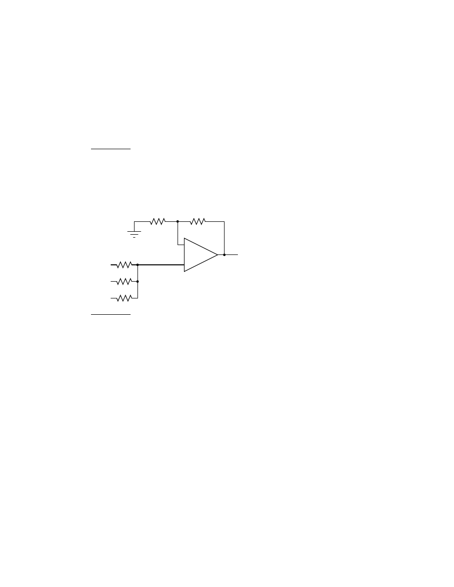
8.4. SPECIFIC TROUBLESHOOTING TECHNIQUES
115
8.4.3
Divide system into sections and test those sections
In a system with multiple sections or stages, carefully measure the variables going in and out of each
stage until you find a stage where things don’t look right.
Example 1: A radio is not working (producing no sound at the speaker))
What to do: Divide the circuitry into stages: tuning stage, mixing stages, amplifier stage, all the
way through to the speaker(s). Measure signals at test points between these stages and tell whether
or not a stage is working properly.
Example 2: An analog summer circuit is not functioning properly.
−
+
V
in1
V
in2
V
in3
V
out
R
R
R
R
2R
Analog summer circuit
What to do: I would test the passive averager network (the three resistors at the lower-left corner
of the schematic) to see that the proper (averaged) voltage was seen at the noninverting input of
the op-amp. I would then measure the voltage at the inverting input to see if it was the same as at
the noninverting input (or, alternatively, measure the voltage difference between the two inputs of
the op-amp, as it should be zero). Continue testing sections of the circuit (or just test points within
the circuit) to see if you measure the expected voltages and currents.
8.4.4
Simplify and rebuild
Closely related to the strategy of dividing a system into sections, this is actually a design and
fabrication technique useful for new circuits, machines, or systems. It’s always easier begin the
design and construction process in little steps, leading to larger and larger steps, rather than to
build the whole thing at once and try to troubleshoot it as a whole.
Suppose that someone were building a custom automobile. He or she would be foolish to bolt
all the parts together without checking and testing components and subsystems as they went along,
expecting everything to work perfectly after it’s all assembled. Ideally, the builder would check the
proper operation of components along the way through the construction process: start and tune the
engine before it’s connected to the drivetrain, check for wiring problems before all the cover panels
are put in place, check the brake system in the driveway before taking it out on the road, etc.
Countless times I’ve witnessed students build a complex experimental circuit and have trouble
getting it to work because they didn’t stop to check things along the way: test all resistors before

116
CHAPTER 8. TROUBLESHOOTING – THEORY AND PRACTICE
plugging them into place, make sure the power supply is regulating voltage adequately before trying
to power anything with it, etc. It is human nature to rush to completion of a project, thinking that
such checks are a waste of valuable time. However, more time will be wasted in troubleshooting a
malfunctioning circuit than would be spent checking the operation of subsystems throughout the
process of construction.
Take the example of the analog summer circuit in the previous section for example: what if it
wasn’t working properly? How would you simplify it and test it in stages? Well, you could reconnect
the op-amp as a basic comparator and see if it’s responsive to differential input voltages, and/or
connect it as a voltage follower (buffer) and see if it outputs the same analog voltage as what is input.
If it doesn’t perform these simple functions, it will never perform its function in the summer circuit!
By stripping away the complexity of the summer circuit, paring it down to an (almost) bare op-amp,
you can test that component’s functionality and then build from there (add resistor feedback and
check for voltage amplification, then add input resistors and check for voltage summing), checking
for expected results along the way.
8.4.5
Trap a signal
Set up instrumentation (such as a datalogger, chart recorder, or multimeter set on ”record” mode)
to monitor a signal over a period of time. This is especially helpful when tracking down intermittent
problems, which have a way of showing up the moment you’ve turned your back and walked away.
This may be essential for proving what happens first in a fast-acting system. Many fast systems
(especially shutdown ”trip” systems) have a ”first out” monitoring capability to provide this kind
of data.
Example #1: A turbine control system shuts automatically in response to an abnormal con-
dition. By the time a technician arrives at the scene to survey the turbine’s condition, however,
everything is in a ”down” state and it’s impossible to tell what signal or condition was responsible
for the initial shutdown, as all operating parameters are now ”abnormal.”
What to do: One technician I knew used a videocamera to record the turbine control panel, so
he could see what happened (by indications on the gauges) first in an automatic-shutdown event.
Simply by looking at the panel after the fact, there was no way to tell which signal shut the turbine
down, but the videotape playback would show what happened in sequence, down to a frame-by-frame
time resolution.
Example #2: An alarm system is falsely triggering, and you suspect it may be due to a specific
wire connection going bad. Unfortunately, the problem never manifests itself while you’re watching
it!
What to do: Many modern digital multimeters are equipped with ”record” settings, whereby
they can monitor a voltage, current, or resistance over time and note whether that measurement
deviates substantially from a regular value. This is an invaluable tool for use in ”intermittent”
electronic system failures.

8.5. LIKELY FAILURES IN PROVEN SYSTEMS
117
8.5
Likely failures in proven systems
The following problems are arranged in order from most likely to least likely, top to bottom. This
order has been determined largely from personal experience troubleshooting electrical and electronic
problems in automotive, industry, and home applications. This order also assumes a circuit or
system that has been proven to function as designed and has failed after substantial operation time.
Problems experienced in newly assembled circuits and systems do not necessarily exhibit the same
probabilities of occurrence.
8.5.1
Operator error
A frequent cause of system failure is error on the part of those human beings operating it. This
cause of trouble is placed at the top of the list, but of course the actual likelihood depends largely on
the particular individuals responsible for operation. When operator error is the cause of a failure, it
is unlikely that it will be admitted prior to investigation. I do not mean to suggest that operators
are incompetent and irresponsible – quite the contrary: these people are often your best teachers
for learning system function and obtaining a history of failure – but the reality of human error
cannot be overlooked. A positive attitude coupled with good interpersonal skills on the part of the
troubleshooter goes a long way in troubleshooting when human error is the root cause of failure.
8.5.2
Bad wire connections
As incredible as this may sound to the new student of electronics, a high percentage of electrical
and electronic system problems are caused by a very simple source of trouble: poor (i.e. open or
shorted) wire connections. This is especially true when the environment is hostile, including such
factors as high vibration and/or a corrosive atmosphere. Connection points found in any variety of
plug-and-socket connector, terminal strip, or splice are at the greatest risk for failure. The category
of ”connections” also includes mechanical switch contacts, which can be thought of as a high-cycle
connector. Improper wire termination lugs (such as a compression-style connector crimped on the
end of a solid wire – a definite faux pas) can cause high-resistance connections after a period of
trouble-free service.
It should be noted that connections in low-voltage systems tend to be far more troublesome
than connections in high-voltage systems. The main reason for this is the effect of arcing across a
discontinuity (circuit break) in higher-voltage systems tends to blast away insulating layers of dirt
and corrosion, and may even weld the two ends together if sustained long enough. Low-voltage
systems tend not to generate such vigorous arcing across the gap of a circuit break, and also tend
to be more sensitive to additional resistance in the circuit. Mechanical switch contacts used in low-
voltage systems benefit from having the recommended minimum wetting current conducted through
them to promote a healthy amount of arcing upon opening, even if this level of current is not
necessary for the operation of other circuit components.
Although open failures tend to more common than shorted failures, ”shorts” still constitute a
substantial percentage of wiring failure modes. Many shorts are caused by degradation of wire
insulation. This, again, is especially true when the environment is hostile, including such factors
as high vibration, high heat, high humidity, or high voltage. It is rare to find a mechanical switch
contact that is failed shorted, except in the case of high-current contacts where contact ”welding”

118
CHAPTER 8. TROUBLESHOOTING – THEORY AND PRACTICE
may occur in overcurrent conditions. Shorts may also be caused by conductive buildup across
terminal strip sections or the backs of printed circuit boards.
A common case of shorted wiring is the ground fault, where a conductor accidently makes contact
with either earth or chassis ground. This may change the voltage(s) present between other conductors
in the circuit and ground, thereby causing bizarre system malfunctions and/or personnel hazard.
8.5.3
Power supply problems
These generally consist of tripped overcurrent protection devices or damage due to overheating.
Although power supply circuitry is usually less complex than the circuitry being powered, and
therefore should figure to be less prone to failure on that basis alone, it generally handles more
power than any other portion of the system and therefore must deal with greater voltages and/or
currents. Also, because of its relative design simplicity, a system’s power supply may not receive the
engineering attention it deserves, most of the engineering focus devoted to more glamorous parts of
the system.
8.5.4
Active components
Active components (amplification devices) tend to fail with greater regularity than passive (non-
amplifying) devices, due to their greater complexity and tendency to amplify overvoltage/overcurrent
conditions. Semiconductor devices are notoriously prone to failure due to electrical transient (volt-
age/current surge) overloading and thermal (heat) overloading. Electron tube devices are far more
resistant to both of these failure modes, but are generally more prone to mechanical failures due to
their fragile construction.
8.5.5
Passive components
Non-amplifying components are the most rugged of all, their relative simplicity granting them a
statistical advantage over active devices. The following list gives an approximate relation of failure
probabilities (again, top being the most likely and bottom being the least likely):
• Capacitors (shorted), especially electrolytic capacitors. The paste electrolyte tends to lose
moisture with age, leading to failure. Thin dielectric layers may be punctured by overvoltage
transients.
• Diodes open (rectifying diodes) or shorted (Zener diodes).
• Inductor and transformer windings open or shorted to conductive core. Failures related to
overheating (insulation breakdown) are easily detected by smell.
• Resistors open, almost never shorted. Usually this is due to overcurrent heating, although it
is less frequently caused by overvoltage transient (arc-over) or physical damage (vibration or
impact). Resistors may also change resistance value if overheated!

8.6. LIKELY FAILURES IN UNPROVEN SYSTEMS
119
8.6
Likely failures in unproven systems
”All men are liable to error;”
John Locke
Whereas the last section deals with component failures in systems that have been successfully
operating for some time, this section concentrates on the problems plaguing brand-new systems. In
this case, failure modes are generally not of the aging kind, but are related to mistakes in design
and assembly caused by human beings.
8.6.1
Wiring problems
In this case, bad connections are usually due to assembly error, such as connection to the wrong
point or poor connector fabrication. Shorted failures are also seen, but usually involve misconnections
(conductors inadvertently attached to grounding points) or wires pinched under box covers.
Another wiring-related problem seen in new systems is that of electrostatic or electromagnetic
interference between different circuits by way of close wiring proximity. This kind of problem is
easily created by routing sets of wires too close to each other (especially routing signal cables close
to power conductors), and tends to be very difficult to identify and locate with test equipment.
8.6.2
Power supply problems
Blown fuses and tripped circuit breakers are likely sources of trouble, especially if the project in
question is an addition to an already-functioning system. Loads may be larger than expected,
resulting in overloading and subsequent failure of power supplies.
8.6.3
Defective components
In the case of a newly-assembled system, component fault probabilities are not as predictable as in
the case of an operating system that fails with age. Any type of component – active or passive – may
be found defective or of imprecise value ”out of the box” with roughly equal probability, barring any
specific sensitivities in shipping (i.e fragile vacuum tubes or electrostatically sensitive semiconductor
components). Moreover, these types of failures are not always as easy to identify by sight or smell
as an age- or transient-induced failure.
8.6.4
Improper system configuration
Increasingly seen in large systems using microprocessor-based components, ”programming” issues
can still plague non-microprocessor systems in the form of incorrect time-delay relay settings,
limit switch calibrations, and drum switch sequences. Complex components having configuration
”jumpers” or switches to control behavior may not be ”programmed” properly.
Components may be used in a new system outside of their tolerable ranges. Resistors, for
example, with too low of power ratings, of too great of tolerance, may have been installed. Sensors,
instruments, and controlling mechanisms may be uncalibrated, or calibrated to the wrong ranges.

120
CHAPTER 8. TROUBLESHOOTING – THEORY AND PRACTICE
8.6.5
Design error
Perhaps the most difficult to pinpoint and the slowest to be recognized (especially by the chief
designer) is the problem of design error, where the system fails to function simply because it cannot
function as designed. This may be as trivial as the designer specifying the wrong components in
a system, or as fundamental as a system not working due to the designer’s improper knowledge of
physics.
I once saw a turbine control system installed that used a low-pressure switch on the lubrication
oil tubing to shut down the turbine if oil pressure dropped to an insufficient level. The oil pressure
for lubrication was supplied by an oil pump turned by the turbine. When installed, the turbine
refused to start. Why? Because when it was stopped, the oil pump was not turning, thus there
was no oil pressure to lubricate the turbine. The low-oil-pressure switch detected this condition and
the control system maintained the turbine in shutdown mode, preventing it from starting. This is a
classic example of a design flaw, and it could only be corrected by a change in the system logic.
While most design flaws manifest themselves early in the operational life of the system, some
remain hidden until just the right conditions exist to trigger the fault. These types of flaws are
the most difficult to uncover, as the troubleshooter usually overlooks the possibility of design error
due to the fact that the system is assumed to be ”proven.” The example of the turbine lubrication
system was a design flaw impossible to ignore on start-up. An example of a ”hidden” design flaw
might be a faulty emergency coolant system for a machine, designed to remain inactive until certain
abnormal conditions are reached – conditions which might never be experienced in the life of the
system.
8.7
Potential pitfalls
Fallacious reasoning and poor interpersonal relations account for more failed or belabored trou-
bleshooting efforts than any other impediments. With this in mind, the aspiring troubleshooter
needs to be familiar with a few common troubleshooting mistakes.
Trusting that a brand-new component will always be good. While it is generally true
that a new component will be in good condition, it is not always true. It is also possible that
a component has been mis-labeled and may have the wrong value (usually this mis-labeling is a
mistake made at the point of distribution or warehousing and not at the manufacturer, but again,
not always!).
Not periodically checking your test equipment. This is especially true with battery-
powered meters, as weak batteries may give spurious readings. When using meters to safety-check
for dangerous voltage, remember to test the meter on a known source of voltage both before and
after checking the circuit to be serviced, to make sure the meter is in proper operating condition.
Assuming there is only one failure to account for the problem. Single-failure system
problems are ideal for troubleshooting, but sometimes failures come in multiple numbers. In some
instances, the failure of one component may lead to a system condition that damages other compo-
nents. Sometimes a component in marginal condition goes undetected for a long time, then when
another component fails the system suffers from problems with both components.

8.7. POTENTIAL PITFALLS
121
Mistaking coincidence for causality. Just because two events occurred at nearly the same
time does not necessarily mean one event caused the other! They may be both consequences of a
common cause, or they may be totally unrelated! If possible, try to duplicate the same condition
suspected to be the cause and see if the event suspected to be the coincidence happens again. If not,
then there is either no causal relationship as assumed. This may mean there is no causal relationship
between the two events whatsoever, or that there is a causal relationship, but just not the one you
expected.
Self-induced blindness. After a long effort at troubleshooting a difficult problem, you may
become tired and begin to overlook crucial clues to the problem. Take a break and let someone
else look at it for a while. You will be amazed at what a difference this can make. On the other
hand, it is generally a bad idea to solicit help at the start of the troubleshooting process. Effective
troubleshooting involves complex, multi-level thinking, which is not easily communicated with others.
More often than not, ”team troubleshooting” takes more time and causes more frustration than doing
it yourself. An exception to this rule is when the knowledge of the troubleshooters is complementary:
for example, a technician who knows electronics but not machine operation, teamed with an operator
who knows machine function but not electronics.
Failing to question the troubleshooting work of others on the same job. This may
sound rather cynical and misanthropic, but it is sound scientific practice. Because it is easy to
overlook important details, troubleshooting data received from another troubleshooter should be
personally verified before proceeding. This is a common situation when troubleshooters ”change
shifts” and a technician takes over for another technician who is leaving before the job is done. It
is important to exchange information, but do not assume the prior technician checked everything
they said they did, or checked it perfectly. I’ve been hindered in my troubleshooting efforts on many
occasions by failing to verify what someone else told me they checked.
Being pressured to ”hurry up.” When an important system fails, there will be pressure
from other people to fix the problem as quickly as possible. As they say in business, ”time is
money.” Having been on the receiving end of this pressure many times, I can understand the need
for expedience. However, in many cases there is a higher priority: caution. If the system in question
harbors great danger to life and limb, the pressure to ”hurry up” may result in injury or death.
At the very least, hasty repairs may result in further damage when the system is restarted. Most
failures can be recovered or at least temporarily repaired in short time if approached intelligently.
Improper ”fixes” resulting in haste often lead to damage that cannot be recovered in short time, if
ever. If the potential for greater harm is present, the troubleshooter needs to politely address the
pressure received from others, and maintain their perspective in the midst of chaos. Interpersonal
skills are just as important in this realm as technical ability!
Finger-pointing. It is all too easy to blame a problem on someone else, for reasons of ignorance,
pride, laziness, or some other unfortunate facet of human nature. When the responsibility for system
maintenance is divided into departments or work crews, troubleshooting efforts are often hindered
by blame cast between groups. ”It’s a mechanical problem . . . it’s an electrical problem . . . it’s
an instrument problem . . .” ad infinitum, ad nauseum, is all too common in the workplace. I have
found that a positive attitude does more to quench the fires of blame than anything else.

122
CHAPTER 8. TROUBLESHOOTING – THEORY AND PRACTICE
On one particular job, I was summoned to fix a problem in a hydraulic system assumed to be
related to the electronic metering and controls. My troubleshooting isolated the source of trouble to
a faulty control valve, which was the domain of the millwright (mechanical) crew. I knew that the
millwright on shift was a contentious person, so I expected trouble if I simply passed the problem on
to his department. Instead, I politely explained to him and his supervisor the nature of the problem
as well as a brief synopsis of my reasoning, then proceeded to help him replace the faulty valve, even
though it wasn’t ”my” responsibility to do so. As a result, the problem was fixed very quickly, and
I gained the respect of the millwright.
8.8
Contributors
Contributors to this chapter are listed in chronological order of their contributions, from most recent
to first. See Appendix 2 (Contributor List) for dates and contact information.
Alejandro Gamero Divasto (January 2002): contributed troubleshooting tips regarding po-
tential hazards of swapping two similar components, avoiding pressure placed on the troubleshooter,
perils of ”team” troubleshooting, wisdom of recording system history, operator error as a cause of
failure, and the perils of finger-pointing.

Chapter 9
CIRCUIT SCHEMATIC
SYMBOLS
Contents
. . . . . . . . . . . . . . . . . . . . . . . . . . . . 124
. . . . . . . . . . . . . . . . . . . . . . . . . . . . . . . . . 125
. . . . . . . . . . . . . . . . . . . . . . . . . . . . . . . . . . . . . 125
. . . . . . . . . . . . . . . . . . . . . . . . . . . . . . . . . . . . 126
. . . . . . . . . . . . . . . . . . . . . . . . . . . . . . . . . . . . 126
. . . . . . . . . . . . . . . . . . . . . . . . . . . . . . . 127
. . . . . . . . . . . . . . . . . . . . . . . . . . . 128
. . . . . . . . . . . . . . . . . . . . . . . . . . 129
Switches, electrically actuated (relays)
. . . . . . . . . . . . . . . . . . 130
. . . . . . . . . . . . . . . . . . . . . . . . . . . . . . . . . . . 130
. . . . . . . . . . . . . . . . . . . . . . . . . . . . . . . . . . . . . . 131
. . . . . . . . . . . . . . . . . . . . . . . . . . . . . . 132
9.13 Transistors, junction field-effect (JFET)
. . . . . . . . . . . . . . . . . . 132
9.14 Transistors, insulated-gate field-effect (IGFET or MOSFET)
. . . . . 133
. . . . . . . . . . . . . . . . . . . . . . . . . . . . . . . 133
. . . . . . . . . . . . . . . . . . . . . . . . . . . . . . . . . . . . 134
. . . . . . . . . . . . . . . . . . . . . . . . . . . . . . . 135
. . . . . . . . . . . . . . . . . . . . . . . . . . . . . . . . . 138
123
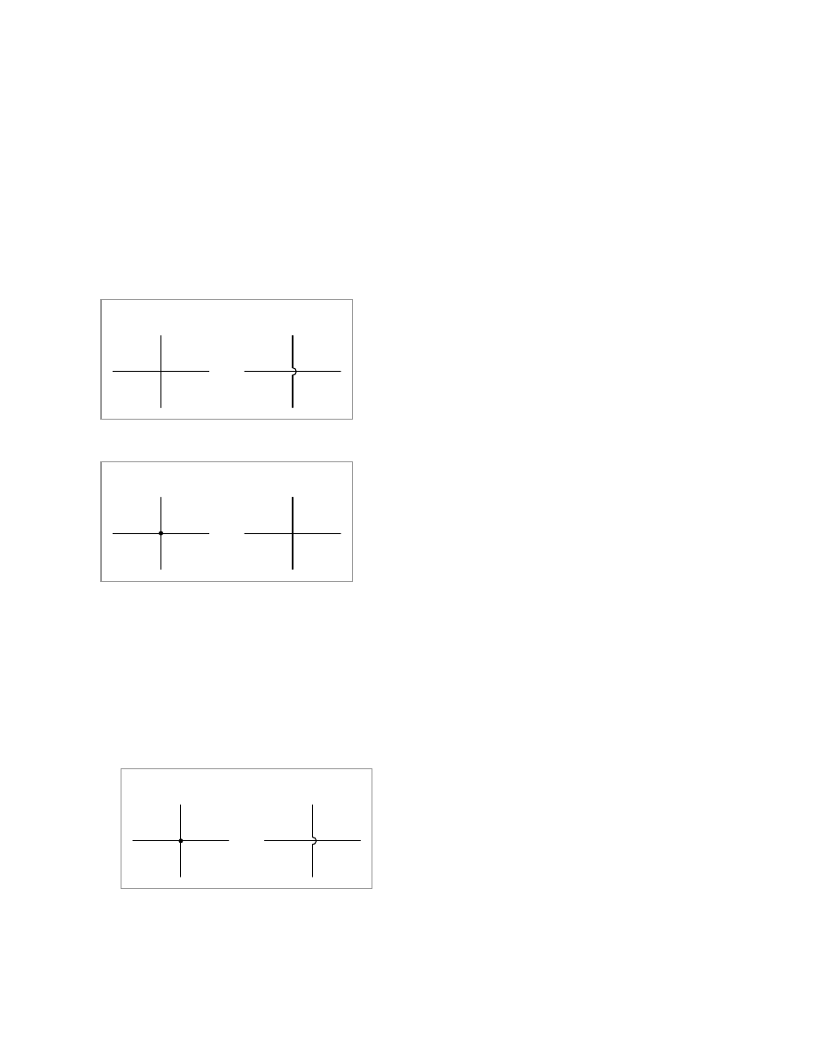
124
CHAPTER 9. CIRCUIT SCHEMATIC SYMBOLS
9.1
Wires and connections
Connected
Not connected
Older convention
Connected
Not connected
Newer convention
Older electrical schematics showed connecting wires crossing, while non-connecting wires ”jumped”
over each other with little half-circle marks. Newer electrical schematics show connecting wires join-
ing with a dot, while non-connecting wires cross with no dot. However, some people still use the
older convention of connecting wires crossing with no dot, which may create confusion.
For this reason, I opt to use a hybrid convention, with connecting wires unambiguously connected
by a dot, and non-connecting wires unambiguously ”jumping” over one another with a half-circle
mark. While this may be frowned upon by some, it leaves no room for interpretational error: in
each case, the intent is clear and unmistakable:
Connected
Not connected
Convention used in this book
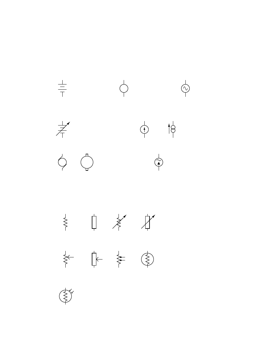
9.2. POWER SOURCES
125
9.2
Power sources
DC voltage
AC voltage
Variable
DC voltage
+
−
DC voltage
A diagonal arrow
represents variability
for any component!
DC current
+
-
Generator
AC current
Gen
9.3
Resistors
Fixed-value
Rheostat
Potentiometer
Tapped
Thermistor
t
o
Photoresistor
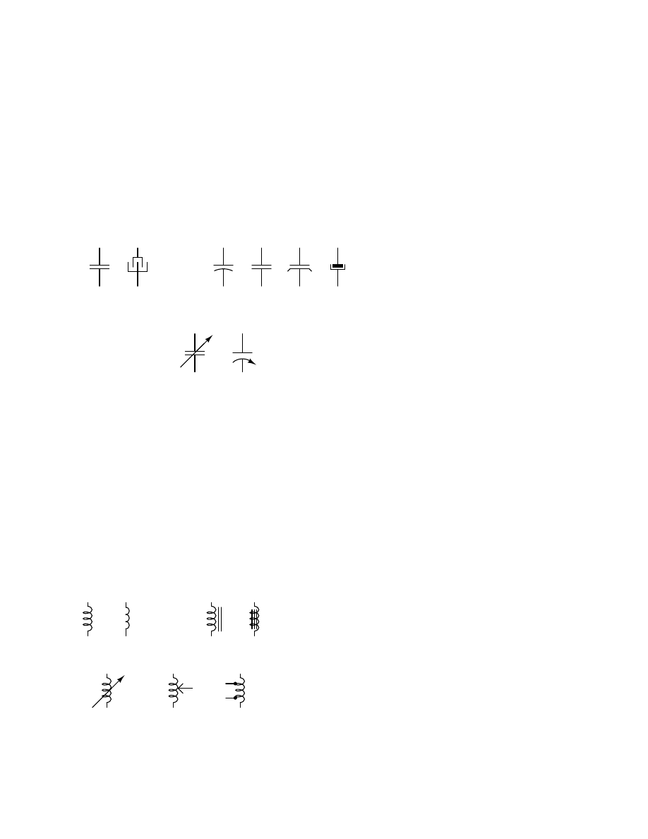
126
CHAPTER 9. CIRCUIT SCHEMATIC SYMBOLS
9.4
Capacitors
Non-polarized
+
Polarized (top positive)
Variable
9.5
Inductors
Fixed-value
Iron core
Tapped
Variable
Variac
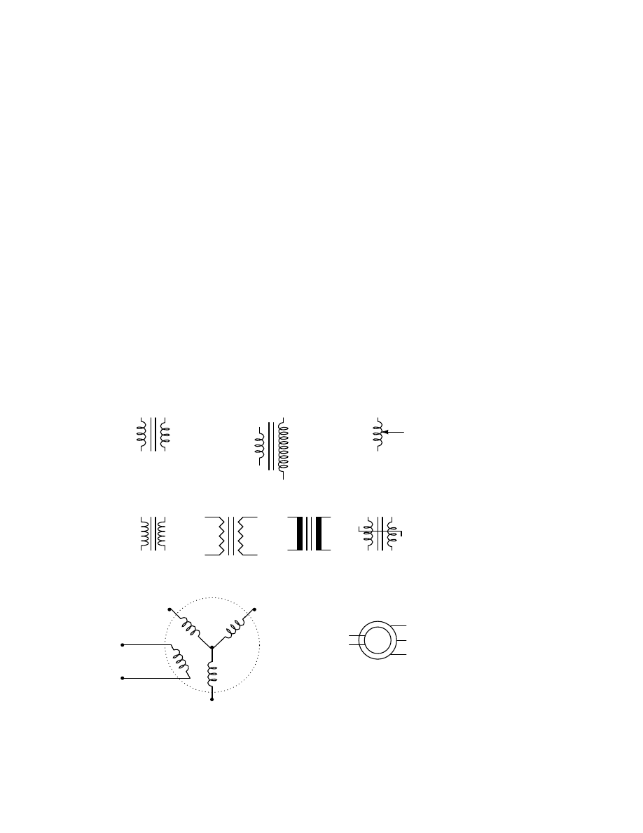
9.6. MUTUAL INDUCTORS
127
9.6
Mutual inductors
Transformer
Step-up/step-down
transformer
Transformer
Transformer
Variac
Saturable
reactor
Synchro
Synchro
Transformer
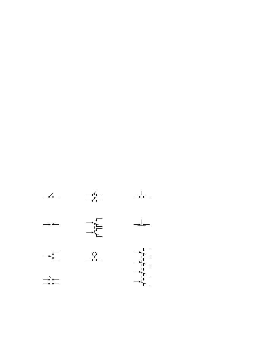
128
CHAPTER 9. CIRCUIT SCHEMATIC SYMBOLS
9.7
Switches, hand actuated
normally open
SPST toggle
SPST toggle
normally closed
SPDT toggle
DPST toggle
DPDT toggle
Pushbutton
normally open
Pushbutton
normally closed
SPST joystick
position of dot
on circle indicates
joystick direction
4PDT toggle
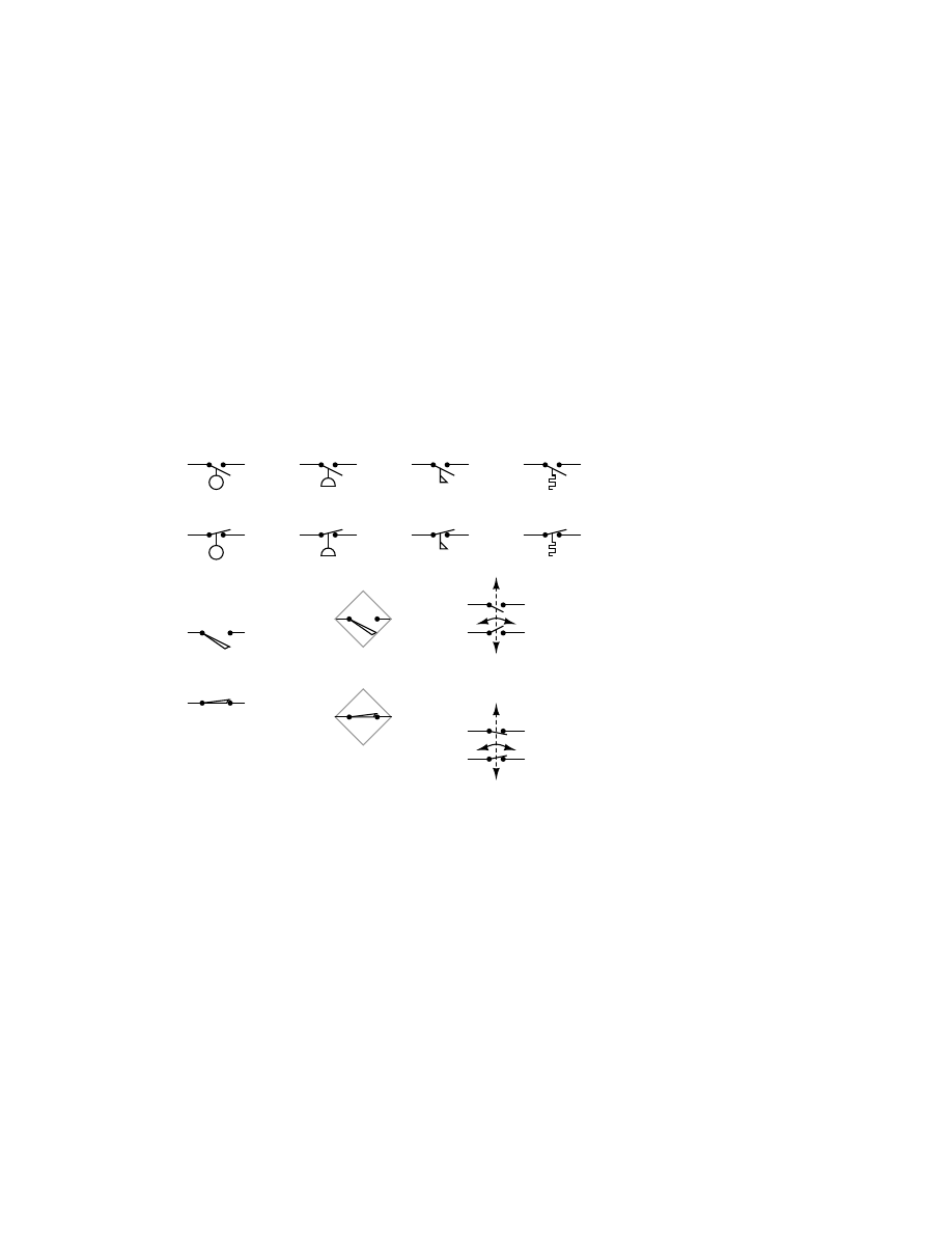
9.8. SWITCHES, PROCESS ACTUATED
129
9.8
Switches, process actuated
Level
Normally open shown on top; normally closed on bottom
Pressure
Temperature
Flow
Limit
Electronic
Limit
F
R
F
R
Speed
It is very important to keep in mind that the ”normal” contact status of a process-actuated
switch refers to its status when the process is absent and/or inactive, not ”normal” in the sense of
process conditions as expected during routine operation. For instance, a normally-closed low-flow
detection switch installed on a coolant pipe will be maintained in the actuated state (open) when
there is regular coolant flow through the pipe. If the coolant flow stops, the flow switch will go to
its ”normal” (unactuated) status of closed.
A limit switch is one actuated by contact with a moving machine part. An electronic limit switch
senses mechanical motion, but does so using light, magnetic fields, or other non-contact means.
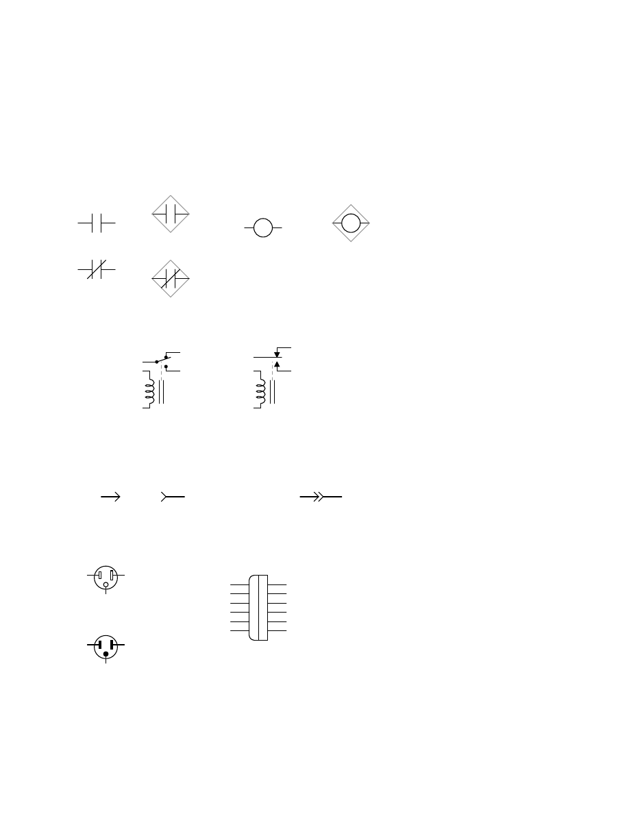
130
CHAPTER 9. CIRCUIT SCHEMATIC SYMBOLS
9.9
Switches, electrically actuated (relays)
Generic
Electronic
Relay coil,
electromechanical
Relay coil,
electronic
Relay components, "ladder logic" notation style
Relays, electronic schematic notation style
9.10
Connectors
Plug
(male)
Jack
(female)
Plug & Jack
connected
Plug
Jack
Multi-conductor
plug/jack set
Receptacle
(female)
Plug
(male)
Household
power
connectors
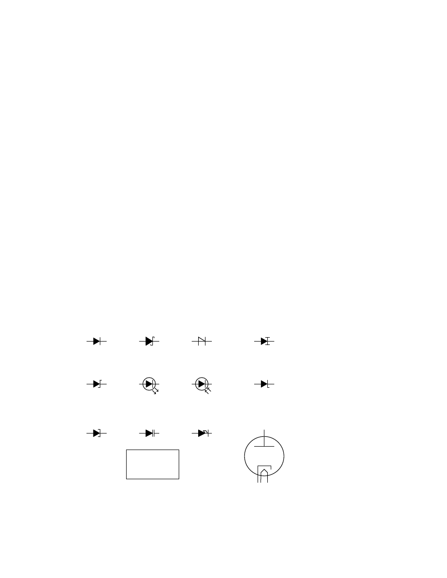
9.11. DIODES
131
9.11
Diodes
Generic
Schottky
Shockley
Constant current
Tunnel
Varactor
PIN
Step recovery
Zener
Light-emitting
Photo-
Tunnel
Vacuum tube
K
A
A
K
A
K
A
K
A
K
A
K
A
K
A
K
A
K
A
K
A
K
P
C
H
1
H
2
A = Anode
K = Cathode
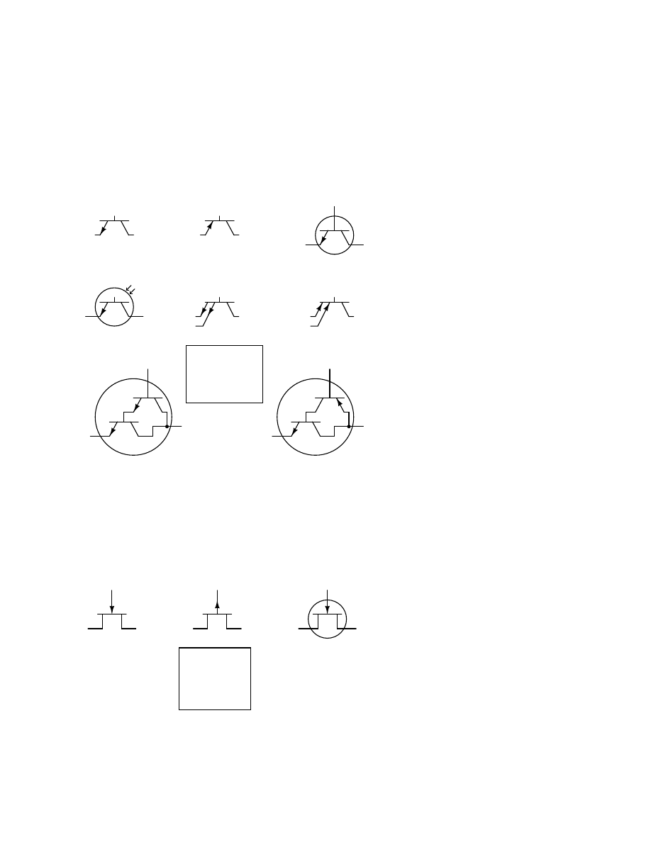
132
CHAPTER 9. CIRCUIT SCHEMATIC SYMBOLS
9.12
Transistors, bipolar
Bipolar NPN
Bipolar PNP
Dual-emitter NPN
Dual-emitter PNP
. . . with case
Darlington pair
Sziklai pair
Photo-
B
C
E
E
C
B
C
B
E
1
E
2
E
1
E
2
B
C
E
C
E
C
B
E
C
B
E = Emitter
B = Base
C = Collector
9.13
Transistors, junction field-effect (JFET)
. . . with case
N-channel
P-channel
G
S
D
G
S
D
S = Source
G = Gate
D = Drain
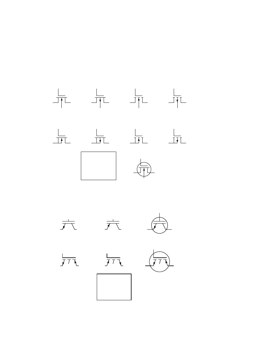
9.14. TRANSISTORS, INSULATED-GATE FIELD-EFFECT (IGFET OR MOSFET)
133
9.14
Transistors, insulated-gate field-effect (IGFET or MOS-
FET)
N-channel
P-channel
G
G
S
S
D
D
SS
SS
S
G
D
N-channel
P-channel
G
S
D
N-channel
P-channel
depletion
depletion
G
S
D
G
S
D
. . . with case
enhancement
enhancement
depletion
depletion
S
G
D
S
G
D
SS
SS
N-channel
enhancement
P-channel
enhancement
S = Source
G = Gate
D = Drain
SS = Substrate
9.15
Transistors, hybrid
. . . with case
IGBT (NPN)
IGBT (PNP)
G
C
E
G
C
E
IGBT (N-channel)
IGBT (P-channel)
. . . with case
E
G
C
G
E
C
E = Emitter
G = Gate
C = Collector
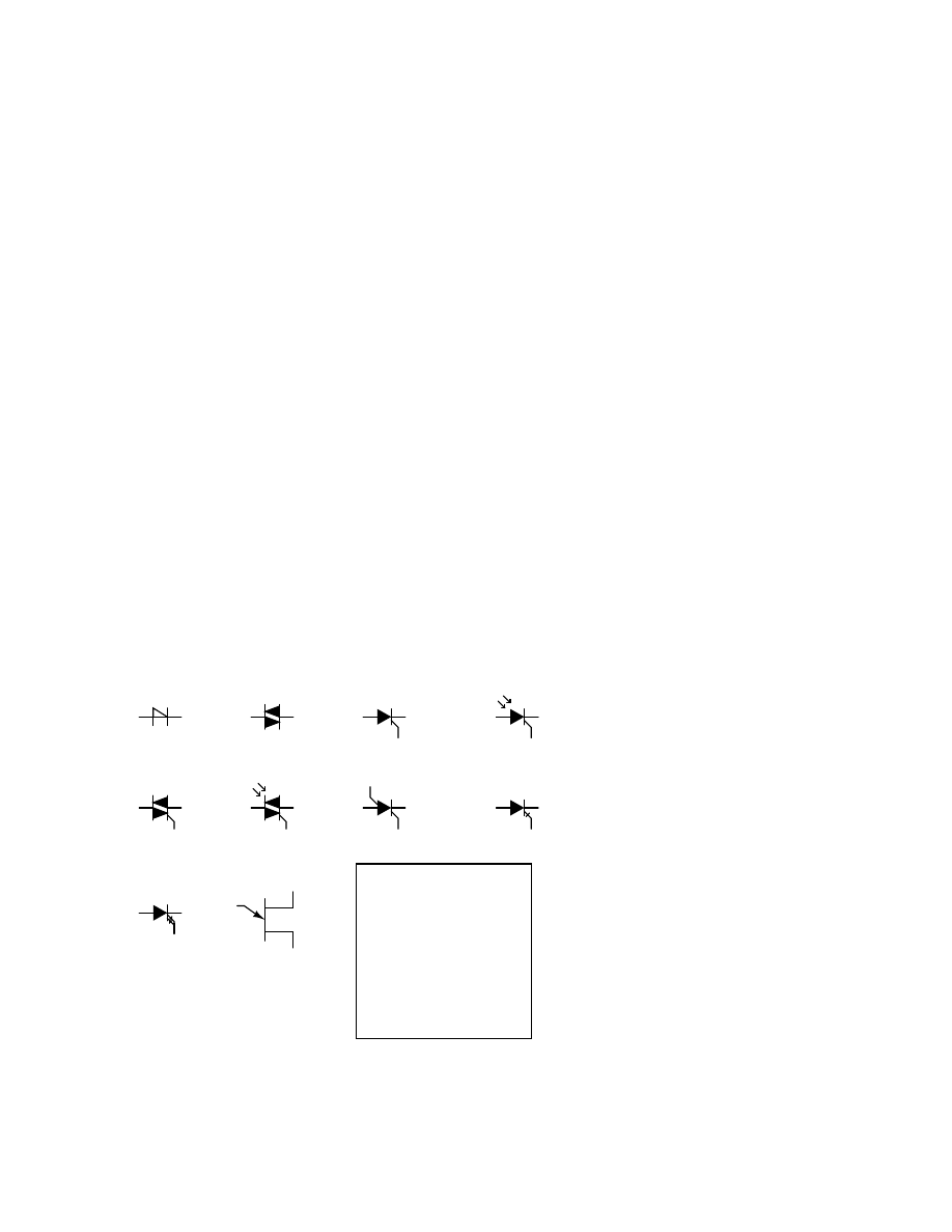
134
CHAPTER 9. CIRCUIT SCHEMATIC SYMBOLS
9.16
Thyristors
Shockley
A
K
DIAC
A
K
G
SCR
A
K
G
LASCR
TRIAC
MT
1
MT
2
G
Opto-TRIAC
MT
2
MT
1
G
A
K
G
A
G
K
SCS
GCS
A
K
G
GTO
A
K
G
UJT
B
1
B
2
E
A = Anode
K = Cathode
G = Gate
E = Emitter
B = Base
MT = Main Terminal
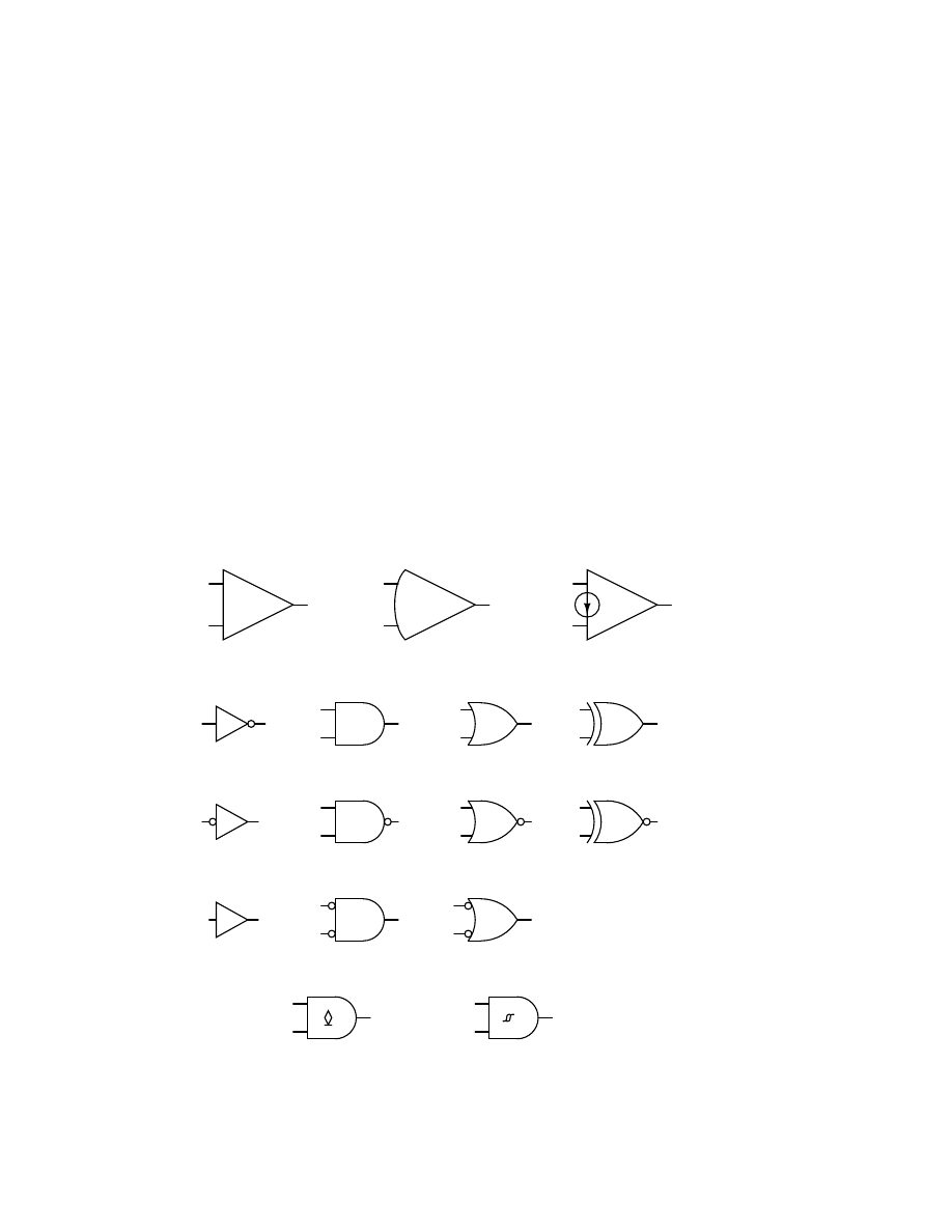
9.17. INTEGRATED CIRCUITS
135
9.17
Integrated circuits
−
+
Operational amplifier
-
+
−
+
(alternative)
Norton op-amp
Inverter
AND gate
OR gate
XOR gate
Inverter
NAND gate
NOR gate
XNOR gate
Buffer
Gate with open-
collector output
Gate with Schmitt
trigger input
Negative-AND
gate
Negative-OR
gate
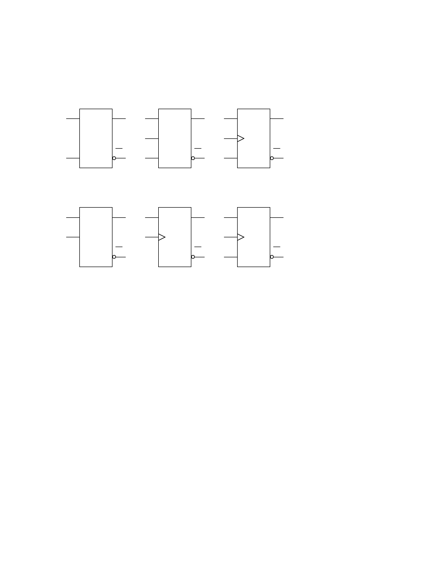
136
CHAPTER 9. CIRCUIT SCHEMATIC SYMBOLS
S
Q
Q
R
S-R Latch
S
Q
Q
R
E
Enabled S-R Latch
S
Q
Q
R
C
S-R Flip-flop
Q
Q
D
E
D Latch
D
C
Q
Q
D Flip-flop
J
Q
Q
C
K
J-K Flip-flop

9.17. INTEGRATED CIRCUITS
137
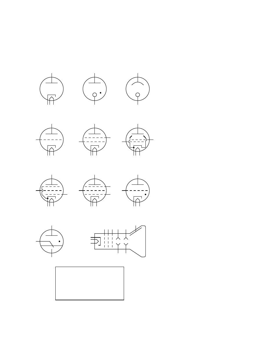
138
CHAPTER 9. CIRCUIT SCHEMATIC SYMBOLS
9.18
Electron tubes
Diode
C
P
H
1
H
2
Glow tube
C
P
C
Phototube
A
Triode
P
C
H
1
H
2
G
G
P
C
H
1
H
2
Tetrode
S
P
C
H
1
H
2
G
S
Beam tetrode
Pentode
P
G
C
H
1
H
2
S
P
S
G
H
2
H
1
C
Sup
Pentode
Thyratron
G
P
C
H
1
H
2
P = Plate
G = Grid
C = Cathode
H = Heater
S = Screen
Sup = Suppressor
A = Anode
Ignitron
A
C
I
I = Ignitor
H
V
Cathode Ray Tube

Chapter 10
PERIODIC TABLE OF THE
ELEMENTS
Contents
. . . . . . . . . . . . . . . . . . . . . . . . . . . . 141
. . . . . . . . . . . . . . . . . . . . . . . . . . . . . 142
. . . . . . . . . . . . . . . . . . . . . . . . . . . . . . . . . . . . . . . 142
139

140
CHAPTER 10. PERIODIC TABLE OF THE ELEMENTS
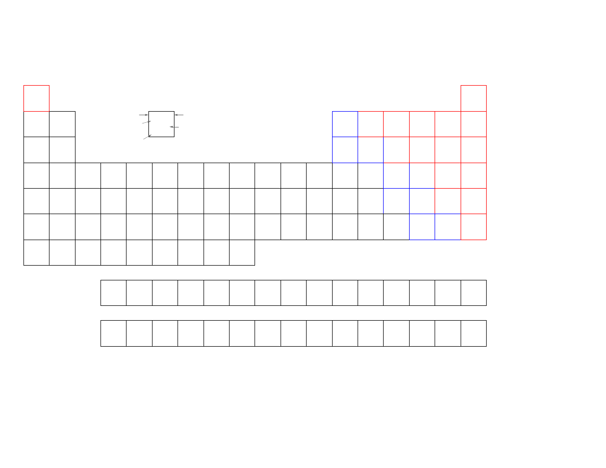
10.1.
T
ABLE
(LANDSCAPE
VIEW)
141
10.1
T
able
(landscap
e
view)
Potassium
K
19
39.0983
4s
1
Calcium
Ca
20
4s
2
Na
Sodium
11
3s
1
Magnesium
Mg
12
3s
2
H
1
Hydrogen
1s
1
Li
Lithium
6.941
3
2s
1
Beryllium
Be
4
2s
2
Sc
21
Scandium
3d
1
4s
2
Ti
22
Titanium
3d
2
4s
2
V
23
Vanadium
50.9415
3d
3
4s
2
Cr
24
Chromium
3d
5
4s
1
Mn
25
Manganese
3d
5
4s
2
Fe
26
Iron
55.847
3d
6
4s
2
Co
27
Cobalt
3d
7
4s
2
Ni
28
Nickel
3d
8
4s
2
Cu
29
Copper
63.546
3d
10
4s
1
Zn
30
Zinc
3d
10
4s
2
Ga
31
Gallium
4p
1
B
5
Boron
10.81
2p
1
C
6
Carbon
12.011
2p
2
N
7
Nitrogen
14.0067
2p
3
O
8
Oxygen
15.9994
2p
4
F
9
Fluorine
18.9984
2p
5
He
2
Helium
4.00260
1s
2
Ne
10
Neon
20.179
2p
6
Ar
18
Argon
39.948
3p
6
Kr
36
Krypton
83.80
4p
6
Xe
54
Xenon
131.30
5p
6
Rn
86
Radon
(222)
6p
6
K
Potassium
19
39.0983
4s
1
Symbol
Atomic number
Name
Atomic mass
Electron
configuration
Al
13
Aluminum
26.9815
3p
1
Si
14
Silicon
28.0855
3p
2
P
15
Phosphorus
30.9738
3p
3
S
16
Sulfur
32.06
3p
4
Cl
17
Chlorine
35.453
3p
5
Periodic Table of the Elements
Germanium
4p
2
Ge
32
As
Arsenic
33
4p
3
Se
Selenium
34
78.96
4p
4
Br
Bromine
35
79.904
4p
5
I
Iodine
53
126.905
5p
5
Rubidium
37
85.4678
5s
1
Sr
Strontium
38
87.62
5s
2
Yttrium
Y
39
4d
1
5s
2
Zr
40
Zirconium
91.224
4d
2
5s
2
Nb
41
Niobium
92.90638
4d
4
5s
1
Mo
42
Molybdenum
95.94
4d
5
5s
1
Tc
43
Technetium
(98)
4d
5
5s
2
Ru
44
Ruthenium
101.07
4d
7
5s
1
Rh
45
Rhodium
4d
8
5s
1
Pd
46
Palladium
106.42
4d
10
5s
0
Ag
47
Silver
107.8682
4d
10
5s
1
Cd
48
Cadmium
112.411
4d
10
5s
2
In
49
Indium
114.82
5p
1
Sn
50
Tin
118.710
5p
2
Sb
51
Antimony
121.75
5p
3
Te
52
Tellurium
127.60
5p
4
Po
84
Polonium
(209)
6p
4
At
Astatine
85
(210)
6p
5
Metals
Metalloids
Nonmetals
Rb
Cs
55
Cesium
132.90543
6s
1
Ba
56
Barium
137.327
6s
2
57 - 71
Lanthanide
series
Hf
72
Hafnium
178.49
5d
2
6s
2
Ta
Tantalum
73
180.9479
5d
3
6s
2
W
74
Tungsten
183.85
5d
4
6s
2
Re
75
Rhenium
186.207
5d
5
6s
2
Os
76
Osmium
190.2
5d
6
6s
2
Ir
77
192.22
Iridium
5d
7
6s
2
Pt
78
Platinum
195.08
5d
9
6s
1
Au
Gold
79
196.96654
5d
10
6s
1
Hg
80
Mercury
200.59
5d
10
6s
2
Tl
81
Thallium
204.3833
6p
1
Pb
Lead
82
207.2
6p
2
Bi
Bismuth
83
208.98037
6p
3
Lanthanide
series
Fr
87
Francium
(223)
7s
1
Ra
88
Radium
(226)
7s
2
89 - 103
Actinide
series
Actinide
series
104
Unq
Unnilquadium
(261)
6d
2
7s
2
Unp
105
Unnilpentium
(262)
6d
3
7s
2
Unh
106
Unnilhexium
(263)
6d
4
7s
2
Uns
107
Unnilseptium
(262)
108
109
1.00794
9.012182
22.989768
24.3050
40.078
44.955910
47.88
51.9961
54.93805
58.93320
58.69
65.39
69.723
72.61
74.92159
88.90585
102.90550
(averaged according to
occurence on earth)
La
57
Lanthanum
138.9055
5d
1
6s
2
Ce
58
Cerium
140.115
4f
1
5d
1
6s
2
Pr
59
Praseodymium
140.90765
4f
3
6s
2
Nd
60
Neodymium
144.24
4f
4
6s
2
Pm
61
Promethium
(145)
4f
5
6s
2
Sm
62
Samarium
150.36
4f
6
6s
2
Eu
63
Europium
151.965
4f
7
6s
2
Gd
64
Gadolinium
157.25
4f
7
5d
1
6s
2
Tb
65
158.92534
Terbium
4f
9
6s
2
Dy
66
Dysprosium
162.50
4f
10
6s
2
Ho
67
Holmium
164.93032
4f
11
6s
2
Er
68
Erbium
167.26
4f
12
6s
2
Tm
69
Thulium
168.93421
4f
13
6s
2
Yb
70
Ytterbium
173.04
4f
14
6s
2
Lu
71
Lutetium
174.967
4f
14
5d
1
6s
2
Ac
Actinium
89
(227)
6d
1
7s
2
Th
90
Thorium
232.0381
6d
2
7s
2
Pa
91
Protactinium
231.03588
5f
2
6d
1
7s
2
U
92
Uranium
238.0289
5f
3
6d
1
7s
2
Np
93
Neptunium
(237)
5f
4
6d
1
7s
2
Pu
94
Plutonium
(244)
5f
6
6d
0
7s
2
Am
95
Americium
(243)
5f
7
6d
0
7s
2
Cm
96
Curium
(247)
5f
7
6d
1
7s
2
Bk
97
Berkelium
(247)
5f
9
6d
0
7s
2
Cf
98
Californium
(251)
5f
10
6d
0
7s
2
Es
99
Einsteinium
(252)
5f
11
6d
0
7s
2
Fm
100
Fermium
(257)
5f
12
6d
0
7s
2
Md
101
Mendelevium
(258)
5f
13
6d
0
7s
2
No
102
Nobelium
(259)
6d
0
7s
2
Lr
103
Lawrencium
(260)
6d
1
7s
2
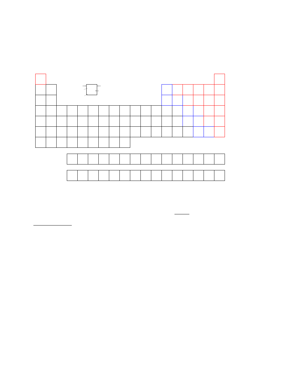
142
CHAPTER 10. PERIODIC TABLE OF THE ELEMENTS
10.2
Table (portrait view)
Potassium
K
19
39.0983
4s
1
Calcium
Ca
20
4s
2
Na
Sodium
11
3s
1
Magnesium
Mg
12
3s
2
H
1
Hydrogen
1s
1
Li
Lithium
6.941
3
2s
1
Beryllium
Be
4
2s
2
Sc
21
Scandium
3d
1
4s
2
Ti
22
Titanium
3d
2
4s
2
V
23
Vanadium
50.9415
3d
3
4s
2
Cr
24
Chromium
3d
5
4s
1
Mn
25
Manganese
3d
5
4s
2
Fe
26
Iron
55.847
3d
6
4s
2
Co
27
Cobalt
3d
7
4s
2
Ni
28
Nickel
3d
8
4s
2
Cu
29
Copper
63.546
3d
10
4s
1
Zn
30
Zinc
3d
10
4s
2
Ga
31
Gallium
4p
1
B
5
Boron
10.81
2p
1
C
6
Carbon
12.011
2p
2
N
7
Nitrogen
14.0067
2p
3
O
8
Oxygen
15.9994
2p
4
F
9
Fluorine
18.9984
2p
5
He
2
Helium
4.00260
1s
2
Ne
10
Neon
20.179
2p
6
Ar
18
Argon
39.948
3p
6
Kr
36
Krypton
83.80
4p
6
Xe
54
Xenon
131.30
5p
6
Rn
86
Radon
(222)
6p
6
K
Potassium
19
39.0983
4s
1
Symbol
Atomic number
Name
Atomic mass
Electron
configuration
Al
13
Aluminum
26.9815
3p
1
Si
14
Silicon
28.0855
3p
2
P
15
Phosphorus
30.9738
3p
3
S
16
Sulfur
32.06
3p
4
Cl
17
Chlorine
35.453
3p
5
Periodic Table of the Elements
Germanium
4p
2
Ge
32
As
Arsenic
33
4p
3
Se
Selenium
34
78.96
4p
4
Br
Bromine
35
79.904
4p
5
I
Iodine
53
126.905
5p
5
Rubidium
37
85.4678
5s
1
Sr
Strontium
38
87.62
5s
2
Yttrium
Y
39
4d
1
5s
2
Zr
40
Zirconium
91.224
4d
2
5s
2
Nb
41
Niobium
92.90638
4d
4
5s
1
Mo
42
Molybdenum
95.94
4d
5
5s
1
Tc
43
Technetium
(98)
4d
5
5s
2
Ru
44
Ruthenium
101.07
4d
7
5s
1
Rh
45
Rhodium
4d
8
5s
1
Pd
46
Palladium
106.42
4d
10
5s
0
Ag
47
Silver
107.8682
4d
10
5s
1
Cd
48
Cadmium
112.411
4d
10
5s
2
In
49
Indium
114.82
5p
1
Sn
50
Tin
118.710
5p
2
Sb
51
Antimony
121.75
5p
3
Te
52
Tellurium
127.60
5p
4
Po
84
Polonium
(209)
6p
4
At
Astatine
85
(210)
6p
5
Metals
Metalloids
Nonmetals
Rb
Cs
55
Cesium
132.90543
6s
1
Ba
56
Barium
137.327
6s
2
57 - 71
Lanthanide
series
Hf
72
Hafnium
178.49
5d
2
6s
2
Ta
Tantalum
73
180.9479
5d
3
6s
2
W
74
Tungsten
183.85
5d
4
6s
2
Re
75
Rhenium
186.207
5d
5
6s
2
Os
76
Osmium
190.2
5d
6
6s
2
Ir
77
192.22
Iridium
5d
7
6s
2
Pt
78
Platinum
195.08
5d
9
6s
1
Au
Gold
79
196.96654
5d
10
6s
1
Hg
80
Mercury
200.59
5d
10
6s
2
Tl
81
Thallium
204.3833
6p
1
Pb
Lead
82
207.2
6p
2
Bi
Bismuth
83
208.98037
6p
3
Lanthanide
series
Fr
87
Francium
(223)
7s
1
Ra
88
Radium
(226)
7s
2
89 - 103
Actinide
series
Actinide
series
104
Unq
Unnilquadium
(261)
6d
2
7s
2
Unp
105
Unnilpentium
(262)
6d
3
7s
2
Unh
106
Unnilhexium
(263)
6d
4
7s
2
Uns
107
Unnilseptium
(262)
108
109
1.00794
9.012182
22.989768
24.3050
40.078
44.955910
47.88
51.9961
54.93805
58.93320
58.69
65.39
69.723
72.61
74.92159
88.90585
102.90550
(averaged according to
occurence on earth)
La
57
Lanthanum
138.9055
5d
1
6s
2
Ce
58
Cerium
140.115
4f
1
5d
1
6s
2
Pr
59
Praseodymium
140.90765
4f
3
6s
2
Nd
60
Neodymium
144.24
4f
4
6s
2
Pm
61
Promethium
(145)
4f
5
6s
2
Sm
62
Samarium
150.36
4f
6
6s
2
Eu
63
Europium
151.965
4f
7
6s
2
Gd
64
Gadolinium
157.25
4f
7
5d
1
6s
2
Tb
65
158.92534
Terbium
4f
9
6s
2
Dy
66
Dysprosium
162.50
4f
10
6s
2
Ho
67
Holmium
164.93032
4f
11
6s
2
Er
68
Erbium
167.26
4f
12
6s
2
Tm
69
Thulium
168.93421
4f
13
6s
2
Yb
70
Ytterbium
173.04
4f
14
6s
2
Lu
71
Lutetium
174.967
4f
14
5d
1
6s
2
Ac
Actinium
89
(227)
6d
1
7s
2
Th
90
Thorium
232.0381
6d
2
7s
2
Pa
91
Protactinium
231.03588
5f
2
6d
1
7s
2
U
92
Uranium
238.0289
5f
3
6d
1
7s
2
Np
93
Neptunium
(237)
5f
4
6d
1
7s
2
Pu
94
Plutonium
(244)
5f
6
6d
0
7s
2
Am
95
Americium
(243)
5f
7
6d
0
7s
2
Cm
96
Curium
(247)
5f
7
6d
1
7s
2
Bk
97
Berkelium
(247)
5f
9
6d
0
7s
2
Cf
98
Californium
(251)
5f
10
6d
0
7s
2
Es
99
Einsteinium
(252)
5f
11
6d
0
7s
2
Fm
100
Fermium
(257)
5f
12
6d
0
7s
2
Md
101
Mendelevium
(258)
5f
13
6d
0
7s
2
No
102
Nobelium
(259)
6d
0
7s
2
Lr
103
Lawrencium
(260)
6d
1
7s
2
10.3
Data
Atomic masses shown in parentheses indicate the most stable isotope (longest half-life) known.
Electron configuration data was taken from Douglas C. Giancoli’s Physics, 3rd edition. Average
atomic masses were taken from Kenneth W. Whitten’s, Kenneth D. Gailey’s, and Raymond E. Davis’
General Chemistry, 3rd edition. In the latter book, the masses were specified as 1985 IUPAC values.

Appendix A-1
CONTRIBUTOR LIST
A-1.1
How to contribute to this book
As a copylefted work, this book is open to revision and expansion by any interested parties. The
only ”catch” is that credit must be given where credit is due. This is a copyrighted work: it is not
in the public domain!
If you wish to cite portions of this book in a work of your own, you must follow the same
guidelines as for any other copyrighted work. Here is a sample from the Design Science License:
The Work is copyright the Author.
All rights to the Work are reserved
by the Author, except as specifically described below. This License
describes the terms and conditions under which the Author permits you
to copy, distribute and modify copies of the Work.
In addition, you may refer to the Work, talk about it, and (as
dictated by "fair use") quote from it, just as you would any
copyrighted material under copyright law.
Your right to operate, perform, read or otherwise interpret and/or
execute the Work is unrestricted; however, you do so at your own risk,
because the Work comes WITHOUT ANY WARRANTY -- see Section 7 ("NO
WARRANTY") below.
If you wish to modify this book in any way, you must document the nature of those modifications
in the ”Credits” section along with your name, and ideally, information concerning how you may be
contacted. Again, the Design Science License:
Permission is granted to modify or sample from a copy of the Work,
producing a derivative work, and to distribute the derivative work
under the terms described in the section for distribution above,
143

144
APPENDIX A-1.
CONTRIBUTOR LIST
provided that the following terms are met:
(a) The new, derivative work is published under the terms of this
License.
(b) The derivative work is given a new name, so that its name or
title can not be confused with the Work, or with a version of
the Work, in any way.
(c) Appropriate authorship credit is given: for the differences
between the Work and the new derivative work, authorship is
attributed to you, while the material sampled or used from
the Work remains attributed to the original Author; appropriate
notice must be included with the new work indicating the nature
and the dates of any modifications of the Work made by you.
Given the complexities and security issues surrounding the maintenance of files comprising this
book, it is recommended that you submit any revisions or expansions to the original author (Tony R.
Kuphaldt). You are, of course, welcome to modify this book directly by editing your own personal
copy, but we would all stand to benefit from your contributions if your ideas were incorporated into
the online ”master copy” where all the world can see it.
A-1.2
Credits
All entries arranged in alphabetical order of surname. Major contributions are listed by individual
name with some detail on the nature of the contribution(s), date, contact info, etc. Minor contri-
butions (typo corrections, etc.) are listed by name only for reasons of brevity. Please understand
that when I classify a contribution as ”minor,” it is in no way inferior to the effort or value of a
”major” contribution, just smaller in the sense of less text changed. Any and all contributions are
gratefully accepted. I am indebted to all those who have given freely of their own knowledge, time,
and resources to make this a better book!
A-1.2.1
Dennis Crunkilton
• Date(s) of contribution(s):October 2005 to present
• Nature of contribution:Ch 1, added permitivity, capacitor and inductor formulas, wire
table; 10/2005.
• Nature of contribution:Ch 1, expanded dielectric table, 10232.eps, copied data from Volume
1, Chapter 13; 10/2005.
• Nature of contribution: Mini table of contents, all chapters except appedicies; html, latex,
ps, pdf; See Devel/tutorial.html; 01/2006.
• Contact at: dcrunkilton(at)att(dot)net

A-1.2. CREDITS
145
A-1.2.2
Alejandro Gamero Divasto
• Date(s) of contribution(s): January 2002
• Nature of contribution: Suggestions related to troubleshooting: caveat regarding swap-
ping two similar components as a troubleshooting tool; avoiding pressure placed on the trou-
bleshooter; perils of ”team” troubleshooting; wisdom of recording system history; operator
error as a cause of failure; and the perils of finger-pointing.
A-1.2.3
Tony R. Kuphaldt
• Date(s) of contribution(s): 1996 to present
• Nature of contribution: Original author.
• Contact at: liec0@lycos.com
A-1.2.4
Your name here
• Date(s) of contribution(s): Month and year of contribution
• Nature of contribution: Insert text here, describing how you contributed to the book.
• Contact at: my email@provider.net
A-1.2.5
Typo corrections and other ”minor” contributions
• The students of Bellingham Technical College’s Instrumentation program.
• Bernard Sheehan (January 2005), Typographical error correction in ”Right triangle trigonom-
etry” section Chapter 5: TRIGONOMETRY REFERENCE (two formulas for tan x the second
one reads tan x = cos x/sin x it should be cot x = cos x/sin x– changes to 01001.eps previously
made)
• Chirvasuta Constantin (April 2003) Identified error in quadratic equation formula.
• Jeff DeFreitas (March 2006)Improve appearance: replace ”/” and ”/” Chapters: A1, A2.
• Gerald Gardner (January 2003) Suggested adding Imperial gallons conversion to table.
• Harvey Lew (??? 2003) Typo correction in Trig chapter: ”tangent” should have been ”cotan-
gent”.
• Don Stalkowski (June 2002) Technical help with PostScript-to-PDF file format conversion.
• Joseph Teichman (June 2002) Suggestion and technical help regarding use of PNG images
instead of JPEG.

146
APPENDIX A-1.
CONTRIBUTOR LIST

Appendix A-2
ABOUT THIS BOOK
A-2.1
Purpose
They say that necessity is the mother of invention. At least in the case of this book, that adage
is true. As an industrial electronics instructor, I was forced to use a sub-standard textbook during
my first year of teaching. My students were daily frustrated with the many typographical errors
and obscure explanations in this book, having spent much time at home struggling to comprehend
the material within. Worse yet were the many incorrect answers in the back of the book to selected
problems. Adding insult to injury was the $100+ price.
Contacting the publisher proved to be an exercise in futility. Even though the particular text I
was using had been in print and in popular use for a couple of years, they claimed my complaint
was the first they’d ever heard. My request to review the draft for the next edition of their book
was met with disinterest on their part, and I resolved to find an alternative text.
Finding a suitable alternative was more difficult than I had imagined. Sure, there were plenty of
texts in print, but the really good books seemed a bit too heavy on the math and the less intimidating
books omitted a lot of information I felt was important. Some of the best books were out of print,
and those that were still being printed were quite expensive.
It was out of frustration that I compiled Lessons in Electric Circuits from notes and ideas I had
been collecting for years. My primary goal was to put readable, high-quality information into the
hands of my students, but a secondary goal was to make the book as affordable as possible. Over the
years, I had experienced the benefit of receiving free instruction and encouragement in my pursuit
of learning electronics from many people, including several teachers of mine in elementary and high
school. Their selfless assistance played a key role in my own studies, paving the way for a rewarding
career and fascinating hobby. If only I could extend the gift of their help by giving to other people
what they gave to me . . .
So, I decided to make the book freely available. More than that, I decided to make it ”open,”
following the same development model used in the making of free software (most notably the various
UNIX utilities released by the Free Software Foundation, and the Linux operating system, whose
fame is growing even as I write). The goal was to copyright the text – so as to protect my authorship
147

148
APPENDIX A-2.
ABOUT THIS BOOK
– but expressly allow anyone to distribute and/or modify the text to suit their own needs with a
minimum of legal encumbrance. This willful and formal revoking of standard distribution limitations
under copyright is whimsically termed copyleft. Anyone can ”copyleft” their creative work simply
by appending a notice to that effect on their work, but several Licenses already exist, covering the
fine legal points in great detail.
The first such License I applied to my work was the GPL – General Public License – of the
Free Software Foundation (GNU). The GPL, however, is intended to copyleft works of computer
software, and although its introductory language is broad enough to cover works of text, its wording
is not as clear as it could be for that application. When other, less specific copyleft Licenses began
appearing within the free software community, I chose one of them (the Design Science License, or
DSL) as the official notice for my project.
In ”copylefting” this text, I guaranteed that no instructor would be limited by a text insufficient
for their needs, as I had been with error-ridden textbooks from major publishers. I’m sure this book
in its initial form will not satisfy everyone, but anyone has the freedom to change it, leveraging my
efforts to suit variant and individual requirements. For the beginning student of electronics, learn
what you can from this book, editing it as you feel necessary if you come across a useful piece of
information. Then, if you pass it on to someone else, you will be giving them something better than
what you received. For the instructor or electronics professional, feel free to use this as a reference
manual, adding or editing to your heart’s content. The only ”catch” is this: if you plan to distribute
your modified version of this text, you must give credit where credit is due (to me, the original
author, and anyone else whose modifications are contained in your version), and you must ensure
that whoever you give the text to is aware of their freedom to similarly share and edit the text. The
next chapter covers this process in more detail.
It must be mentioned that although I strive to maintain technical accuracy in all of this book’s
content, the subject matter is broad and harbors many potential dangers. Electricity maims and
kills without provocation, and deserves the utmost respect. I strongly encourage experimentation
on the part of the reader, but only with circuits powered by small batteries where there is no risk of
electric shock, fire, explosion, etc. High-power electric circuits should be left to the care of trained
professionals! The Design Science License clearly states that neither I nor any contributors to this
book bear any liability for what is done with its contents.
A-2.2
The use of SPICE
One of the best ways to learn how things work is to follow the inductive approach: to observe
specific instances of things working and derive general conclusions from those observations. In
science education, labwork is the traditionally accepted venue for this type of learning, although
in many cases labs are designed by educators to reinforce principles previously learned through
lecture or textbook reading, rather than to allow the student to learn on their own through a truly
exploratory process.
Having taught myself most of the electronics that I know, I appreciate the sense of frustration
students may have in teaching themselves from books. Although electronic components are typically
inexpensive, not everyone has the means or opportunity to set up a laboratory in their own homes,
and when things go wrong there’s no one to ask for help. Most textbooks seem to approach the task
of education from a deductive perspective: tell the student how things are supposed to work, then
apply those principles to specific instances that the student may or may not be able to explore by

A-2.3. ACKNOWLEDGEMENTS
149
themselves. The inductive approach, as useful as it is, is hard to find in the pages of a book.
However, textbooks don’t have to be this way. I discovered this when I started to learn a
computer program called SPICE. It is a text-based piece of software intended to model circuits and
provide analyses of voltage, current, frequency, etc. Although nothing is quite as good as building
real circuits to gain knowledge in electronics, computer simulation is an excellent alternative. In
learning how to use this powerful tool, I made a discovery: SPICE could be used within a textbook
to present circuit simulations to allow students to ”observe” the phenomena for themselves. This
way, the readers could learn the concepts inductively (by interpreting SPICE’s output) as well as
deductively (by interpreting my explanations). Furthermore, in seeing SPICE used over and over
again, they should be able to understand how to use it themselves, providing a perfectly safe means
of experimentation on their own computers with circuit simulations of their own design.
Another advantage to including computer analyses in a textbook is the empirical verification
it adds to the concepts presented. Without demonstrations, the reader is left to take the author’s
statements on faith, trusting that what has been written is indeed accurate. The problem with
faith, of course, is that it is only as good as the authority in which it is placed and the accuracy
of interpretation through which it is understood. Authors, like all human beings, are liable to err
and/or communicate poorly. With demonstrations, however, the reader can immediately see for
themselves that what the author describes is indeed true. Demonstrations also serve to clarify the
meaning of the text with concrete examples.
SPICE is introduced early in volume I (DC) of this book series, and hopefully in a gentle enough
way that it doesn’t create confusion. For those wishing to learn more, a chapter in this volume
(volume V) contains an overview of SPICE with many example circuits. There may be more flashy
(graphic) circuit simulation programs in existence, but SPICE is free, a virtue complementing the
charitable philosophy of this book very nicely.
A-2.3
Acknowledgements
First, I wish to thank my wife, whose patience during those many and long evenings (and weekends!)
of typing has been extraordinary.
I also wish to thank those whose open-source software development efforts have made this en-
deavor all the more affordable and pleasurable. The following is a list of various free computer
software used to make this book, and the respective programmers:
• GNU/Linux Operating System – Linus Torvalds, Richard Stallman, and a host of others too
numerous to mention.
• Vim text editor – Bram Moolenaar and others.
• Xcircuit drafting program – Tim Edwards.
• SPICE circuit simulation program – too many contributors to mention.
• TEX text processing system – Donald Knuth and others.
• Texinfo document formatting system – Free Software Foundation.
• L
A
TEX document formatting system – Leslie Lamport and others.

150
APPENDIX A-2.
ABOUT THIS BOOK
• Gimp image manipulation program – too many contributors to mention.
Appreciation is also extended to Robert L. Boylestad, whose first edition of Introductory Circuit
Analysis taught me more about electric circuits than any other book. Other important texts in
my electronics studies include the 1939 edition of The ”Radio” Handbook, Bernard Grob’s second
edition of Introduction to Electronics I, and Forrest Mims’ original Engineer’s Notebook.
Thanks to the staff of the Bellingham Antique Radio Museum, who were generous enough to let
me terrorize their establishment with my camera and flash unit.
I wish to specifically thank Jeffrey Elkner and all those at Yorktown High School for being willing
to host my book as part of their Open Book Project, and to make the first effort in contributing to its
form and content. Thanks also to David Sweet (website: (http://www.andamooka.org)) and Ben
Crowell (website: (http://www.lightandmatter.com)) for providing encouragement, constructive
criticism, and a wider audience for the online version of this book.
Thanks to Michael Stutz for drafting his Design Science License, and to Richard Stallman for
pioneering the concept of copyleft.
Last but certainly not least, many thanks to my parents and those teachers of mine who saw in
me a desire to learn about electricity, and who kindled that flame into a passion for discovery and
intellectual adventure. I honor you by helping others as you have helped me.
Tony Kuphaldt, July 2001
”A candle loses nothing of its light when lighting another”
Kahlil Gibran

Appendix A-3
CONTRIBUTOR LIST
A-3.1
How to contribute to this book
As a copylefted work, this book is open to revision and expansion by any interested parties. The
only ”catch” is that credit must be given where credit is due. This is a copyrighted work: it is not
in the public domain!
If you wish to cite portions of this book in a work of your own, you must follow the same
guidelines as for any other copyrighted work. Here is a sample from the Design Science License:
The Work is copyright the Author.
All rights to the Work are reserved
by the Author, except as specifically described below. This License
describes the terms and conditions under which the Author permits you
to copy, distribute and modify copies of the Work.
In addition, you may refer to the Work, talk about it, and (as
dictated by "fair use") quote from it, just as you would any
copyrighted material under copyright law.
Your right to operate, perform, read or otherwise interpret and/or
execute the Work is unrestricted; however, you do so at your own risk,
because the Work comes WITHOUT ANY WARRANTY -- see Section 7 ("NO
WARRANTY") below.
If you wish to modify this book in any way, you must document the nature of those modifications
in the ”Credits” section along with your name, and ideally, information concerning how you may be
contacted. Again, the Design Science License:
Permission is granted to modify or sample from a copy of the Work,
producing a derivative work, and to distribute the derivative work
under the terms described in the section for distribution above,
151

152
APPENDIX A-3.
CONTRIBUTOR LIST
provided that the following terms are met:
(a) The new, derivative work is published under the terms of this
License.
(b) The derivative work is given a new name, so that its name or
title can not be confused with the Work, or with a version of
the Work, in any way.
(c) Appropriate authorship credit is given: for the differences
between the Work and the new derivative work, authorship is
attributed to you, while the material sampled or used from
the Work remains attributed to the original Author; appropriate
notice must be included with the new work indicating the nature
and the dates of any modifications of the Work made by you.
Given the complexities and security issues surrounding the maintenance of files comprising this
book, it is recommended that you submit any revisions or expansions to the original author (Tony R.
Kuphaldt). You are, of course, welcome to modify this book directly by editing your own personal
copy, but we would all stand to benefit from your contributions if your ideas were incorporated into
the online “master copy” where all the world can see it.
A-3.2
Credits
All entries arranged in alphabetical order of surname. Major contributions are listed by individual
name with some detail on the nature of the contribution(s), date, contact info, etc. Minor contri-
butions (typo corrections, etc.) are listed by name only for reasons of brevity. Please understand
that when I classify a contribution as “minor,” it is in no way inferior to the effort or value of a
“major” contribution, just smaller in the sense of less text changed. Any and all contributions are
gratefully accepted. I am indebted to all those who have given freely of their own knowledge, time,
and resources to make this a better book!
A-3.2.1
Dennis Crunkilton
• Date(s) of contribution(s):October 2005 to present
• Nature of contribution:Ch 1, added permitivity, capacitor and inductor formulas, wire
table; 10/2005.
• Nature of contribution:Ch 1, expanded dielectric table, 10232.eps, copied data from Volume
1, Chapter 13; 10/2005.
• Nature of contribution: Mini table of contents, all chapters except appedicies; html, latex,
ps, pdf; See Devel/tutorial.html; 01/2006.
• Contact at: dcrunkilton(at)att(dot)net

A-3.2. CREDITS
153
A-3.2.2
Alejandro Gamero Divasto
• Date(s) of contribution(s): January 2002
• Nature of contribution: Suggestions related to troubleshooting: caveat regarding swap-
ping two similar components as a troubleshooting tool; avoiding pressure placed on the trou-
bleshooter; perils of ”team” troubleshooting; wisdom of recording system history; operator
error as a cause of failure; and the perils of finger-pointing.
A-3.2.3
Tony R. Kuphaldt
• Date(s) of contribution(s): 1996 to present
• Nature of contribution: Original author.
• Contact at: liec0@lycos.com
A-3.2.4
Your name here
• Date(s) of contribution(s): Month and year of contribution
• Nature of contribution: Insert text here, describing how you contributed to the book.
• Contact at: my email@provider.net
A-3.2.5
Typo corrections and other “minor” contributions
• The students of Bellingham Technical College’s Instrumentation program.
• Bernard Sheehan (January 2005), Typographical error correction in ”Right triangle trigonom-
etry” section Chapter 5: TRIGONOMETRY REFERENCE (two formulas for tan x the second
one reads tan x = cos x/sin x it should be cot x = cos x/sin x– changes to 01001.eps previously
made)
• Chirvasuta Constantin (April 2003) Identified error in quadratic equation formula.
• Jeff DeFreitas (March 2006)Improve appearance: replace “/” and ”/” Chapters: A1, A2.
• Gerald Gardner (January 2003) Suggested adding Imperial gallons conversion to table.
• Harvey Lew (??? 2003) Typo correction in Trig chapter: ”tangent” should have been ”cotan-
gent”.
• Don Stalkowski (June 2002) Technical help with PostScript-to-PDF file format conversion.
• Joseph Teichman (June 2002) Suggestion and technical help regarding use of PNG images
instead of JPEG.

154
APPENDIX A-3.
CONTRIBUTOR LIST

Appendix A-4
DESIGN SCIENCE LICENSE
Contents
. . . . . . . . . . . . . . . . . . . . . . . . . . . . . . . . . . . 155
. . . . . . . . . . . . . . . . . . . . . . . . . . . . . . . . . . 156
. . . . . . . . . . . . . . . . . . . . . . . . . . . . 156
A-4.43. Copying and distribution
. . . . . . . . . . . . . . . . . . . . . . . . . 156
. . . . . . . . . . . . . . . . . . . . . . . . . . . . . . . . . 157
. . . . . . . . . . . . . . . . . . . . . . . . . . . . . . . 157
. . . . . . . . . . . . . . . . . . . . . . . . . . . . . . . . . 157
. . . . . . . . . . . . . . . . . . . . . . . . . . . . . . . . . 158
A-4.98. Disclaimer of liability
. . . . . . . . . . . . . . . . . . . . . . . . . . . 158
Copyright c
° 1999-2000 Michael Stutz stutz@dsl.org
Verbatim copying of this document is permitted, in any medium.
A-4.1
0. Preamble
Copyright law gives certain exclusive rights to the author of a work, including the rights to copy,
modify and distribute the work (the ”reproductive,” ”adaptative,” and ”distribution” rights).
The idea of ”copyleft” is to willfully revoke the exclusivity of those rights under certain terms
and conditions, so that anyone can copy and distribute the work or properly attributed derivative
works, while all copies remain under the same terms and conditions as the original.
The intent of this license is to be a general ”copyleft” that can be applied to any kind of work
that has protection under copyright. This license states those certain conditions under which a work
published under its terms may be copied, distributed, and modified.
Whereas ”design science” is a strategy for the development of artifacts as a way to reform the
environment (not people) and subsequently improve the universal standard of living, this Design
Science License was written and deployed as a strategy for promoting the progress of science and
art through reform of the environment.
155

156
APPENDIX A-4.
DESIGN SCIENCE LICENSE
A-4.2
1. Definitions
”License” shall mean this Design Science License. The License applies to any work which contains
a notice placed by the work’s copyright holder stating that it is published under the terms of this
Design Science License.
”Work” shall mean such an aforementioned work. The License also applies to the output of
the Work, only if said output constitutes a ”derivative work” of the licensed Work as defined by
copyright law.
”Object Form” shall mean an executable or performable form of the Work, being an embodiment
of the Work in some tangible medium.
”Source Data” shall mean the origin of the Object Form, being the entire, machine-readable,
preferred form of the Work for copying and for human modification (usually the language, encoding
or format in which composed or recorded by the Author); plus any accompanying files, scripts or
other data necessary for installation, configuration or compilation of the Work.
(Examples of ”Source Data” include, but are not limited to, the following: if the Work is an
image file composed and edited in ’PNG’ format, then the original PNG source file is the Source
Data; if the Work is an MPEG 1.0 layer 3 digital audio recording made from a ’WAV’ format audio
file recording of an analog source, then the original WAV file is the Source Data; if the Work was
composed as an unformatted plaintext file, then that file is the the Source Data; if the Work was
composed in LaTeX, the LaTeX file(s) and any image files and/or custom macros necessary for
compilation constitute the Source Data.)
”Author” shall mean the copyright holder(s) of the Work.
The individual licensees are referred to as ”you.”
A-4.3
2. Rights and copyright
The Work is copyright the Author. All rights to the Work are reserved by the Author, except
as specifically described below. This License describes the terms and conditions under which the
Author permits you to copy, distribute and modify copies of the Work.
In addition, you may refer to the Work, talk about it, and (as dictated by ”fair use”) quote from
it, just as you would any copyrighted material under copyright law.
Your right to operate, perform, read or otherwise interpret and/or execute the Work is unre-
stricted; however, you do so at your own risk, because the Work comes WITHOUT ANY WAR-
RANTY – see Section 7 (”NO WARRANTY”) below.
A-4.4
3. Copying and distribution
Permission is granted to distribute, publish or otherwise present verbatim copies of the entire Source
Data of the Work, in any medium, provided that full copyright notice and disclaimer of warranty,
where applicable, is conspicuously published on all copies, and a copy of this License is distributed
along with the Work.
Permission is granted to distribute, publish or otherwise present copies of the Object Form of
the Work, in any medium, under the terms for distribution of Source Data above and also provided
that one of the following additional conditions are met:

A-4.5. 4. MODIFICATION
157
(a) The Source Data is included in the same distribution, distributed under the terms of this
License; or
(b) A written offer is included with the distribution, valid for at least three years or for as long
as the distribution is in print (whichever is longer), with a publicly-accessible address (such as a
URL on the Internet) where, for a charge not greater than transportation and media costs, anyone
may receive a copy of the Source Data of the Work distributed according to the section above; or
(c) A third party’s written offer for obtaining the Source Data at no cost, as described in para-
graph (b) above, is included with the distribution. This option is valid only if you are a non-
commercial party, and only if you received the Object Form of the Work along with such an offer.
You may copy and distribute the Work either gratis or for a fee, and if desired, you may offer
warranty protection for the Work.
The aggregation of the Work with other works which are not based on the Work – such as but
not limited to inclusion in a publication, broadcast, compilation, or other media – does not bring
the other works in the scope of the License; nor does such aggregation void the terms of the License
for the Work.
A-4.5
4. Modification
Permission is granted to modify or sample from a copy of the Work, producing a derivative work,
and to distribute the derivative work under the terms described in the section for distribution above,
provided that the following terms are met:
(a) The new, derivative work is published under the terms of this License.
(b) The derivative work is given a new name, so that its name or title can not be confused with
the Work, or with a version of the Work, in any way.
(c) Appropriate authorship credit is given: for the differences between the Work and the new
derivative work, authorship is attributed to you, while the material sampled or used from the Work
remains attributed to the original Author; appropriate notice must be included with the new work
indicating the nature and the dates of any modifications of the Work made by you.
A-4.6
5. No restrictions
You may not impose any further restrictions on the Work or any of its derivative works beyond those
restrictions described in this License.
A-4.7
6. Acceptance
Copying, distributing or modifying the Work (including but not limited to sampling from the Work
in a new work) indicates acceptance of these terms. If you do not follow the terms of this License,
any rights granted to you by the License are null and void. The copying, distribution or modification
of the Work outside of the terms described in this License is expressly prohibited by law.
If for any reason, conditions are imposed on you that forbid you to fulfill the conditions of this
License, you may not copy, distribute or modify the Work at all.
If any part of this License is found to be in conflict with the law, that part shall be interpreted
in its broadest meaning consistent with the law, and no other parts of the License shall be affected.

158
APPENDIX A-4.
DESIGN SCIENCE LICENSE
A-4.8
7. No warranty
THE WORK IS PROVIDED ”AS IS,” AND COMES WITH ABSOLUTELY NO WARRANTY,
EXPRESS OR IMPLIED, TO THE EXTENT PERMITTED BY APPLICABLE LAW, INCLUD-
ING BUT NOT LIMITED TO THE IMPLIED WARRANTIES OF MERCHANTABILITY OR
FITNESS FOR A PARTICULAR PURPOSE.
A-4.9
8. Disclaimer of liability
IN NO EVENT SHALL THE AUTHOR OR CONTRIBUTORS BE LIABLE FOR ANY DIRECT,
INDIRECT, INCIDENTAL, SPECIAL, EXEMPLARY, OR CONSEQUENTIAL DAMAGES (IN-
CLUDING, BUT NOT LIMITED TO, PROCUREMENT OF SUBSTITUTE GOODS OR SER-
VICES; LOSS OF USE, DATA, OR PROFITS; OR BUSINESS INTERRUPTION) HOWEVER
CAUSED AND ON ANY THEORY OF LIABILITY, WHETHER IN CONTRACT, STRICT LI-
ABILITY, OR TORT (INCLUDING NEGLIGENCE OR OTHERWISE) ARISING IN ANY WAY
OUT OF THE USE OF THIS WORK, EVEN IF ADVISED OF THE POSSIBILITY OF SUCH
DAMAGE.
END OF TERMS AND CONDITIONS
[$Id:
dsl.txt,v 1.25 2000/03/14 13:14:14 m Exp m $]

Index
.end command, SPICE,
Electronics Workbench,
Addition method, simultaneous equations,
Adjacent,
Algebraic identities,
Ampacity,
Analysis, AC, SPICE,
Analysis, DC, SPICE,
Analysis, Fourier, SPICE,
Analysis, transient, SPICE,
Antiderivative of e functions,
Antiderivatives,
Arithmetic sequence,
BASIC, computer language,
C, computer language,
Capacitance equation,
Capacitors, SPICE,
Common difference,
Common ratio,
Compiler,
Component names, SPICE,
Conductor ampacity,
Constants, mathematical,
Conversion factor,
Cosines, law of,
Critical temperature, superconductors,
Current measurement, SPICE,
Current sources, AC, SPICE,
Current sources, DC, SPICE,
Current sources, dependent, SPICE,
Current sources, pulse, SPICE,
Derivative of e functions,
Derivative of a constant,
Derivative of power and log functions,
Derivative rules,
Dielectric strength,
Difference, common,
Differential Equations,
Diodes, SPICE,
E, symbol for voltage,
Factor, conversion,
Factorial,
Factoring,
Fault, ground,
FORTRAN, computer language,
Gage size, wire,
General solution,
Geometric sequence,
Ground fault,
Hyperbolic functions,
Hypotenuse,
I, symbol for current,
Impedance,
Independent variable,
Inductance equation,
Inductors, SPICE,
Integral, definite,
Integral, indefinite,
Interpreter,
Joule’s Law,
Law of cosines,
Law of sines,
Limits, calculus,
Logarithm,
Metric prefixes, SPICE,
159

160
INDEX
Metric system,
Model, SPICE,
Mutual inductance, SPICE,
Netlist, SPICE,
Nodes, SPICE,
Ohm’s Law,
Ohm’s Law, AC,
Open circuits, SPICE,
Opposite,
Option, itl5, SPICE,
Option, limpts, SPICE,
Option, list, SPICE,
Option, method, SPICE,
Option, nopage, SPICE,
Option, numdgt, SPICE,
Option, width, SPICE,
Options, miscellaneous, SPICE,
P, symbol for power,
Parallel circuits,
Particular solution,
PASCAL, computer language,
Periodic table,
Plot output, SPICE,
Power factor,
Prefix, metric,
Print output, SPICE,
Programming, SPICE,
Properties, arithmetic,
Properties, exponents,
Properties, radicals ,
Pythagorean Theorem,
Quadratic formula,
R, symbol for resistance,
Radian,
Ratio, common,
Reactance,
Resistance, specific,
Resistance, temperature coefficient of,
Resistor color codes,
Resistors, SPICE,
Resonance,
Rules for antiderivatives,
Scientific notation, SPICE,
Semiconductor model, SPICE,
Sequences,
Series circuits,
Simultaneous equations,
Sines, law of,
Slide rule,
Specific resistance,
SPICE,
SPICE programming,
SPICE2g6,
Substitution method, simultaneous equations,
Superconductivity,
Systems of linear equations,
Temperature coefficient of resistance,
Temperature, critical, for superconductors,
Time constant equations,
Transform function, definition of,
Transformers, SPICE,
Transistors, bipolar, SPICE,
Transistors, jfet, SPICE,
Transistors, mosfet, SPICE,
Trigonometric derivatives ,
Trigonometric equivalencies,
Trigonometric identities,
Troubleshooting,
Unit, radian,
Voltage sources, AC, SPICE,
Voltage sources, DC, SPICE,
Voltage sources, dependent, SPICE,
Voltage sources, pulse, SPICE,
Wetting current,
Wire size, gage scale,
Document Outline
- USEFUL EQUATIONS AND CONVERSION FACTORS
- RESISTOR COLOR CODES
- CONDUCTOR AND INSULATOR TABLES
- ALGEBRA REFERENCE
- TRIGONOMETRY REFERENCE
- CALCULUS REFERENCE
- USING THE SPICE CIRCUIT SIMULATION PROGRAM
- TROUBLESHOOTING -- THEORY AND PRACTICE
- CIRCUIT SCHEMATIC SYMBOLS
- PERIODIC TABLE OF THE ELEMENTS
- CONTRIBUTOR LIST
- ABOUT THIS BOOK
- CONTRIBUTOR LIST
- DESIGN SCIENCE LICENSE
Wyszukiwarka
Podobne podstrony:
Lessons In Electric Circuits, Volume V Reference
A Course of Lessons in Coptic Language
Lessons in the Unfoldment of the Philosophers Stone
Breakthrough An Amazing Experiment in Electronic Communication with the Dead by Konstantin Raudive
US Patent 611,719 Electrical Circuit Controller
elpenor second lesson in ancient greek (voices tenses verb translating) PART 1
US Patent 609,249 Electric Circuit Controller
Human sacrifirce in India, Folklore vol 33, no 1
Sachs Symmetry In Electrodynamics
BJCCFSB2006 346 V3i Keypad Heating Wrong Capacitor Placed in EL Circuit
ALASTAIR GALBRAITH MATT DE GENARRO Long Wires in Dark Museums Vol 2 CD (Table Of The Elements) XER1
Practical Lessons In Yoga practical
Parker Sloan A Lesson In Truth
US Patent 609,248 Electric Circuit Controller
Bearden Slides Visual Tour of what they don t want you to know about electrical circuits (www chen
więcej podobnych podstron