
A Brief Introduction To Mathematica
Dr. Christopher Moretti
Department of Mathematics
Southeastern Oklahoma State University
Mathematica is a registered trademark of Wolfram Research, Inc.

1
TABLE OF CONTENTS
Page
Chapter One - Getting Started
. . . . . . . . . . . . . . . . . . . . . . . . . . . . . . . . . . . . . . . . . . . . . . . . . . . . . . . . . . . . .
3
Section One - Starting Mathematica
. . . . . . . . . . . . . . . . . . . . . . . . . . . . . . . . . . . . . . . . . . . . . . . . . . . .
3
Section Two - Input and Output
. . . . . . . . . . . . . . . . . . . . . . . . . . . . . . . . . . . . . . . . . . . . . . . . . . . . . . .
3
Section Three - Brackets and Braces
. . . . . . . . . . . . . . . . . . . . . . . . . . . . . . . . . . . . . . . . . . . . . . . . . . .
5
Section Four - Exact and Approximate numbers and Built-in Constants
. . . . . . . . . . . . . . . . .
5
Section Five - Loading in Additional Packages
. . . . . . . . . . . . . . . . . . . . . . . . . . . . . . . . . . . . . . . . . .
5
Chapter One Exercises
. . . . . . . . . . . . . . . . . . . . . . . . . . . . . . . . . . . . . . . . . . . . . . . . . . . . . . . . . . . . . . . . .
7
Chapter Two - Mathematical Functions
. . . . . . . . . . . . . . . . . . . . . . . . . . . . . . . . . . . . . . . . . . . . . . . . . . . . .
8
Section One - Built-In Functions
. . . . . . . . . . . . . . . . . . . . . . . . . . . . . . . . . . . . . . . . . . . . . . . . . . . . . . .
8
Section Two - Defining Functions and Equalities
. . . . . . . . . . . . . . . . . . . . . . . . . . . . . . . . . . . . . .
10
Chapter Two Exercises
. . . . . . . . . . . . . . . . . . . . . . . . . . . . . . . . . . . . . . . . . . . . . . . . . . . . . . . . . . . . . . .
12
Chapter Three - Lists and Matrices
. . . . . . . . . . . . . . . . . . . . . . . . . . . . . . . . . . . . . . . . . . . . . . . . . . . . . . . .
13
Section One - Lists
. . . . . . . . . . . . . . . . . . . . . . . . . . . . . . . . . . . . . . . . . . . . . . . . . . . . . . . . . . . . . . . . . . .
13
Section Two - Generating Lists
. . . . . . . . . . . . . . . . . . . . . . . . . . . . . . . . . . . . . . . . . . . . . . . . . . . . . . . .
13
Section Three - Functions Involving Lists
. . . . . . . . . . . . . . . . . . . . . . . . . . . . . . . . . . . . . . . . . . . . . .
14
Section Four - Displaying Tables and Matrices
. . . . . . . . . . . . . . . . . . . . . . . . . . . . . . . . . . . . . . . . .
15
Section Five - Plugging Into Expressions
. . . . . . . . . . . . . . . . . . . . . . . . . . . . . . . . . . . . . . . . . . . . . .
15
Chapter Three Exercises
. . . . . . . . . . . . . . . . . . . . . . . . . . . . . . . . . . . . . . . . . . . . . . . . . . . . . . . . . . . . . .
17
Chapter Four - Mathematica and Algebra
. . . . . . . . . . . . . . . . . . . . . . . . . . . . . . . . . . . . . . . . . . . . . . . . .
18
Chapter Four Exercises
. . . . . . . . . . . . . . . . . . . . . . . . . . . . . . . . . . . . . . . . . . . . . . . . . . . . . . . . . . . . . . .
19
Chapter Five - Solving Equations
. . . . . . . . . . . . . . . . . . . . . . . . . . . . . . . . . . . . . . . . . . . . . . . . . . . . . . . . . .
20
Chapter Five Exercises
. . . . . . . . . . . . . . . . . . . . . . . . . . . . . . . . . . . . . . . . . . . . . . . . . . . . . . . . . . . . . . . .
22
Chapter Six - Calculus
. . . . . . . . . . . . . . . . . . . . . . . . . . . . . . . . . . . . . . . . . . . . . . . . . . . . . . . . . . . . . . . . . . . .
23
Section One - Limits
. . . . . . . . . . . . . . . . . . . . . . . . . . . . . . . . . . . . . . . . . . . . . . . . . . . . . . . . . . . . . . . . . .
23
Section Two - Derivatives
. . . . . . . . . . . . . . . . . . . . . . . . . . . . . . . . . . . . . . . . . . . . . . . . . . . . . . . . . . . . .
23

2
Section Three - Integrals
. . . . . . . . . . . . . . . . . . . . . . . . . . . . . . . . . . . . . . . . . . . . . . . . . . . . . . . . . . . . . .
25
Section Four - Series
. . . . . . . . . . . . . . . . . . . . . . . . . . . . . . . . . . . . . . . . . . . . . . . . . . . . . . . . . . . . . . . . . .
26
Section Five - Differential Equations
. . . . . . . . . . . . . . . . . . . . . . . . . . . . . . . . . . . . . . . . . . . . . . . . . .
27
Chapter Six Exercises
. . . . . . . . . . . . . . . . . . . . . . . . . . . . . . . . . . . . . . . . . . . . . . . . . . . . . . . . . . . . . . . . .
29
Chapter Seven - Linear Algebra
. . . . . . . . . . . . . . . . . . . . . . . . . . . . . . . . . . . . . . . . . . . . . . . . . . . . . . . . . . .
30
Chapter Seven Exercises
. . . . . . . . . . . . . . . . . . . . . . . . . . . . . . . . . . . . . . . . . . . . . . . . . . . . . . . . . . . . . .
32
Chapter Eight - Two-Dimensional Plots
. . . . . . . . . . . . . . . . . . . . . . . . . . . . . . . . . . . . . . . . . . . . . . . . . . .
33
Section One - Basic Plots
. . . . . . . . . . . . . . . . . . . . . . . . . . . . . . . . . . . . . . . . . . . . . . . . . . . . . . . . . . . . .
33
Section Two - Plot Options
. . . . . . . . . . . . . . . . . . . . . . . . . . . . . . . . . . . . . . . . . . . . . . . . . . . . . . . . . . .
33
Section Three - Parametric Plots
. . . . . . . . . . . . . . . . . . . . . . . . . . . . . . . . . . . . . . . . . . . . . . . . . . . . . .
37
Section Four - Plotting the Graphs of Equations
. . . . . . . . . . . . . . . . . . . . . . . . . . . . . . . . . . . . . . .
38
Chapter Eight Exercises
. . . . . . . . . . . . . . . . . . . . . . . . . . . . . . . . . . . . . . . . . . . . . . . . . . . . . . . . . . . . . .
39
Chapter Nine - Three-Dimensional Plots
. . . . . . . . . . . . . . . . . . . . . . . . . . . . . . . . . . . . . . . . . . . . . . . . . . .
40
Section One - Basic 3-D Plots
. . . . . . . . . . . . . . . . . . . . . . . . . . . . . . . . . . . . . . . . . . . . . . . . . . . . . . . . .
40
Section Two - Plot3D Options
. . . . . . . . . . . . . . . . . . . . . . . . . . . . . . . . . . . . . . . . . . . . . . . . . . . . . . . .
41
Section Three - Parametric 3D Plots
. . . . . . . . . . . . . . . . . . . . . . . . . . . . . . . . . . . . . . . . . . . . . . . . . .
45
Chapter Nine Exercises
. . . . . . . . . . . . . . . . . . . . . . . . . . . . . . . . . . . . . . . . . . . . . . . . . . . . . . . . . . . . . . .
48
Solutions to Exercises
. . . . . . . . . . . . . . . . . . . . . . . . . . . . . . . . . . . . . . . . . . . . . . . . . . . . . . . . . . . . . . . . . . . . .
49

3
Chapter One - Getting Started
Section One - Starting Mathematica
To launch the Mathematica application, open its folder and double-click the Mathematica icon.
This will launch the portion of Mathematica known as the front end.
Mathematica is split up into two pieces - the front end and the kernel.
The front end is where you enter commands and where the results are displayed (be they plots,
functions, whatever). The front end is similar to a word processor - it has no mathematical abilities
itself, but it can open, save, and display Mathematica files (called notebooks). You do all of your
work in the front end.
The kernel is where all of the mathematical computation is done. You never actually see the
kernel at work (unless you open a special window to do so), even though that’s where the real work
is being done.
Mathematica is split up this way to conserve computer resources - especially computer memory.
Mathematica’s kernel is very powerful and can tax older computers. Since the front end is separate
from the kernel, you can use the front end to enter things and view previous work without taxing
the computer. When you double-click the Mathematica icon, it launches the front end. The kernel
isn’t launched until you try to evaluate your first expression.
Section Two - Input and Output
In the front end, information is grouped into “cell”. A cell includes both the input and the
output that is generated it by it. Cells are grouped together by square brackets on the right-hand
side of the front end’s window. To evaluate a cell (that is, have Mathematica process it), make
sure your cursor is somewhere in the input portion of the cell (usually the topmost bracket in
the grouping) and hit shift-enter (Windows) or enter (Macintosh). Throughout this text I will
mention “entering” a command, or “using” or “running” a command. All of these mean putting
the command into a cell and then evaluating the cell.
Once evaluated, each command you input (and you can have more than one in a cell) and its
result are assigned numbers so you can refer to them later - the k-th command you enter is labeled
In[k] and its output as Out[k]. For example, type 1+3 in a cell and evaluate it. You should see the

4
input and output numbers on the left side of the front end’s window. In a new cell, type the output
number (if it was Out[2], then type Out[2] in the new cell) and then evaluate the cell. You should
get 4 again, since Mathematica knows you’re referring to the previous calculation. Mathematica
does not go through all the work the second time, it just repeats the output - which can save a lot
of time if the calculation you’re skipping was complex. You don’t have to just repeat the previous
output, you can use it in a new calculation - if you enter 5*Out[2] and evaluate (assuming Out[2]
was the number 4 from before), then Mathematica will return 20.
Another way to refer to previous input is through percent signs. Entering % in Mathematica
is short-hand for “the last output you gave me”. So if the last output was 8128, if you evaluate a
cell with % in it you will get 8128. If you had entered %-5, you would get 8123. So the percent
sign is a good way to quickly refer to your previous calculations without a lot of retyping (or a lot
of cutting-and-pasting). You can even refer to outputs farther back by using more percent signs,
like %% and %%%. If the last three outputs were
x
2
− 2x + 1, 3x, and 5, then if the very next cell
you evaluate is %%% Mathematica will return
x
2
− 2x + 1. One thing you do need to be careful
about is that the percent signs always work in chronological order. If you do 50 calculations in
a notebook and then create a new cell all the way at the top (by clicking the mouse before the
first cell and starting to type) with %%, the result will still be the 49th (second to last) output.
Another thing to be careful of is that if you save a notebook and quit Mathematica, it forgets all
of the previous input and output - both in the In[ ]/Out[ ] format and with percent signs. When
you reopen the notebook you will have to go back and reevaluate the necessary cells the next time
- and if you are using percent signs, you have to do it in the same order too. So if you are going to
be saving your work to disk, retyping output or using copy and paste is not a bad idea.
There is another output trick which occasionally comes in handy. Sometimes you may want
to do a calculation (maybe expanding (
x + 1)
1000
or doing a complex 3-D plot) and not want to
see the output because it would be too long or Mathematica is low on memory. If you end the
input with a semi-colon Mathematica will process the input but won’t print the output. You can
still refer to it by Out[42] or %%% - it just won’t be on the screen. So if you evaluate a cell with
Expand[(
x + 1)
1000
− x
1000
]; Mathematica will still process it, but the output (which would be
several screens long) won’t appear to clutter your work.

5
Section Three - Brackets and Braces
In Mathematica, different ways of grouping things have very different and specific notations.
Parentheses ( ) are used like we normally use them in expressions like 3*(2+1) or (x-2)(x+1).
Square brackets [ ] always belong to functions (built-in functions in Mathematica always start
with capital letters, and sometimes have capital letters for each first letter in a compound word).
Curly brackets
{ } are used for defining lists and matrices.
Section Four - Exact and Approximate numbers and Built-in Constants
In Mathematica, all numbers are considered exact numbers unless you tell it otherwise. 2+3
is the exact number 5 - not 5.0 or 5.00. Even fractions like
1
3
are considered exact.
If you wish to get a numerical estimate of a number, there are two ways to get it. The first
is to follow the number by //N. This will get you the first 6 digits of the number - evaluating 1/3
//N gets you 0.333333. Another (more flexible) way of estimating a number (say 1/3) is to enter
N[1/3]. This will get you 0.333333 again. However, if you want the first 20 digits of 1/3, you simply
alter this to N[1/3,20]. If you wanted the first thousand digits, you would enter N[1/3, 1000].
Mathematica has a number of built-in constants - numbers which come up so often they get
their own notation. Like virtually all built-in objects they start with capital letters. Here are a few
of the more important ones.
Pi - the number
π
≈ 3.14159
E - Euler’s number
e
≈ 2.71828
I - the imaginary number
i =
√
−1
Degree - the number of radians in one degree (
π
180
)
Infinity -
∞.
So if you wanted the first 10000 digits of
π, you would enter N[Pi,10000].
Section Five - Loading Additional Packages
There are many packages of additional functions for Mathematica - add-ons which cover func-
tions and areas not built into the main program. These can be loaded in if you know the name of the
package and the file path the package is in. For example, to load the information contained in the

6
package ImplicitPlot under the heading Graphics, you would enter
<<Graphics`ImplicitPlot`(you
must use the accent sign ` when loading a package - the open quote ‘ won’t work). The
<<
tells Mathematica to load a package, Graphics is the file path and ImplicitPlot is the name of the
package. After evaluating this command, you can now use the commands defined in the package as
if it were part of the program from the start. If you quit and restart Mathematica, you will have
to reload the package (and any others you may have loaded).

7
Chapter One Exercises
1) Use Mathematica and numerical approximation to find which is bigger:
e
π
or
π
e
. Powers
in Mathematica are entered as the ˆ symbol.
2) Using Mathematica, find
i
2
, i
3
, i
4
, i
5
, and i
6
.
3) What are the first 15 digits of
e?
4) Load in the the packages ImplicitPlot and Polyhedra, which can both be found in the file
path Graphics.
5) Try to load in the package ThisIsNotARealPackage from the file path Algebra (which is a
real file path with several packages for extending Mathematica’s algebraic abilities).

8
Chapter Two - Mathematical Functions
Section One - Built-In Functions
Mathematica has several thousand common mathematical functions built into it covering ev-
erything from elementary algebra to advanced functions from real analysis and number theory.
Here is a list of common functions and their notations. If you ever want information on a function,
simply enter a question mark before its name and evaluate that cell. For example, if I wanted to
know what the function Cos[ ] is for, I would evaluate ?Cos. If I wanted technical information (like
special options), I would evaluate ??Cos. If you are not sure of the name of a function, you can
use a * symbol as a “wild card”. If I wanted to know the names of all functions starting with
Cos, I would enter ?Cos*. You can even use more than one wildcard - ?C*s* gives the names of
all functions starting with C with an s in them. Throughout this text I will refer to functions
by putting [ ] after their name, like Cos[ ] or Plot[ ]. When you use the functions in Mathematica
you will have to fill in the appropriate information between the brackets (like Cos[x] or Cos[3Pi]) -
this is just some shorthand which will make it easy to refer to functions. All functions use square
brackets around their arguments.
Arithmetic Notation
Addition: Use the + symbol.
Subtraction: Use the - symbol.
Multiplication: Use either * or a space. Be careful when using spaces - Mathematica interprets
xy not as x*y but a single variable whose name is “xy”.
Division: Use the / symbol.
Exponents: Use the ˆ symbol (2
3
= 2ˆ3). For fractional exponents, use parentheses - for 81
1
/4
,
evaluate 81ˆ(1/4).
Absolute Value: Abs[x] is the absolute value of x. This works for complex numbers as well as
real numbers.
Sign[x]: The sign of x: 1 if x
>0, -1 if x<0, 0 if x=0.
Square roots: Sqrt[x] is the square root of x.
Factorials: n! is the factorial of n (3! will give you 6, 7! will give 5040). If you inadvertently

9
try to take the factorial of something which is not a whole number, Mathematica will return an
expression involving the Gamma[ ] function, which extends the factorial idea to non-whole numbers.
Binomials: Binomial[n,k] gives the binomial coefficient
µ
n
k
, the number of subsets of k
objects from a set of n objects.
One thing you need to be careful of is taking odd roots of negative numbers. If you enter
(-8)ˆ(1/3) in Mathematica, it will return a complex root of -8 rather than -2. You can get around
this using Sign[ ] and Abs[ ] as Sign[-8] Abs[-8]ˆ(1/3).
Trigonometric Functions
In Mathematica, all trigonometric functions and their inverses use radian measure for angles.
So if you want to find the sine of 180 degrees you will need to include the conversion factor Degree
as Sin[180 Degree]. Remember, Mathematica will return exact numbers if exact numbers are given
as input - so Sin[2] is simply Sin[2] unless you numerically approximate it. Mathematica knows
how to use complex numbers with trigonometric functions - so if you inadvertently enter something
which you think of as undefined - like the inverse sine of 2 - you may get a complex answer (you
will usually need to numerically approximate to see this).
Sin[x]: The sine of x
ArcSin[x]: The inverse sine of x.
Cos[x]: The cosine of x
ArcCos[x]: The inverse cosine of x.
Tan[x]: The tangent of x
ArcTan[x]: The inverse tangent of x.
Cot[x]: The cotangent of x
ArcCot[x]: The inverse cotangent of x.
Sec[x]: The secant of x
ArcSec[x]: The inverse secant of x.
Csc[x]: The cosecant of x
ArcCsc[x]: The inverse cosecant of x.
Exponential and Logarithmic Functions
Again, Mathematica can process complex numbers, so you may see unexpected things if you
try to do things like take logarithms of negative numbers.
Exp[x]: The natural exponential function
e
x
(this can also be obtained by Eˆx).
Log[x]: The natural logarithm of x. This differs from standard notation ln(x).
Log[b,x]: the logarithm of x in the base b. So the “common logarithm” of x is Log[10,x].
Hyperbolic Functions
The hyperbolic functions as their inverses are defined in terms of exponentials and logarithms -
so complex numbers are valid arguments and may appear as output from these (if you try to find the

10
inverse hyperbolic cosine of 0, for example) - although you may need to numerically approximate
the values to see this.
Sinh[x]: The hyperbolic sine of x
ArcSinh[x]: The inverse hyperbolic sine of x.
Cosh[x]: The hyperbolic cosine of x
ArcCosh[x]: The inverse hyperbolic cosine of x.
Tanh[x]: The hyperbolic tangent of x
ArcTanh[x]: The inverse hyperbolic tangent of x.
Coth[x]: The hyperbolic cotangent of x
ArcCoth[x]: The inverse hyperbolic cotangent of x.
Sech[x]: The hyperbolic secant of x
ArcSech[x]: The inverse hyperbolic secant of x.
Csch[x]: The hyperbolic cosecant of x
ArcCsch[x]: The inverse hyperbolic cosecant of x.
Section Two - Defining Functions and Equalities
When working with Mathematica, it is often useful to define your own functions, like f(x)=
x
2
−
√
xe
sin(2
x)
. Mathematica has a special notation for equalities which define functions. To define the
function f(x) above, you would enter
f[x ]:=xˆ2-Sqrt[x] Exp[Sin[2x]]
The special equality symbol := is used for defining functions (think of it as “let what comes
before this symbol be”). When you define functions, you must use square brackets. Also notice the
underscore following the x on the right - this means that whatever you enter for x is plugged into the
formula on the right-hand side (whether it is a number or some expression involving variables like
t+1). Once you have evaluated this, you can then evaluate expressions like f[2], f[Cos[t]], f[x+h],
or even f[Bob]. If your function is a pure numerical function like f(x)=x
2
, then you can omit the
: in the function definition - f[x ]=xˆ2 will work just fine (and it will print out the definition of
your function so you can check it). However, if you want to include a Mathematica command as
part of your function - like Expand[xˆ2] for example - you must include the : in the definition
(f[x ]:=Expand[xˆ2]). Omitting the : in this case won’t define the right function - Mathematica
will still square numbers, but won’t “Expand” inputs like (x+h).
You can define functions of more than one variable in the same way. To define g(x,y)=
xy
−
sin(
x ln(y)), you would evaluate g[x ,y ]:=x y-Sin[x Log[y]]. Notice the space between x and y in
the first term and between x and Log[y] in the second - both stand for multiplication. We can now
plug numbers into this function (say x=1 and y=e/2) by evaluating g[1,E/2].
At some point you may wish to redefine a function. While usually just redefining a function
will work, once you get into more complicated functions and programming this may cause some
problems (parts of the old definition may conflict with parts of the new one). The best way to

11
do this is to remove the old definitions before entering the new one. This can be done with the
Clear[ ] command. To eliminate the definition for g(x,y) above, you would evaluate Clear[g]. This
command removes all definitions for g, so this eliminates the possibility of conflicting definitions.
It is tempting to drop the brackets and underscores and just enter something like f=xˆ2 for
the function f(x)=
x
2
. This means something different than defining a function in Mathematica.
You have now defined f to be the “object”
x
2
− 1 - that is, f is now a nickname for the expression
x
2
− 1. You cannot plug numbers into this (at least not directly). You can do other things to it -
you could construct a plot of f as x goes from -3 to 4, take the derivative of f, and try to factor f.
But it’s no longer a function - f just becomes a convenient way to refer to
x
2
− 1. This nicknaming
can be undone just like function definitions by entering Clear[f].
Another thing to watch out for is the notations of equations in algebra. When we have an
equation like 2x+3y=5 in algebra (defining a line, for example), this equation can be either true
or false depending on what values of x and y you plug in (it’s true when x=1 and y=1 but false if
both are 0). This type of equation (one which is true or false rather than referring to the definition
of a function or a nickname) has a different symbol in Mathematica. You would represent this
true/false type of equation with ==. The equation above would be entered as 2x+3y==5. This
comes up with the Solve[ ] command which is used to find solutions to equations. Entering 1==2
yields the output False, whereas 4==2ˆ2 gives True.

12
Chapter Two Exercises
1) What is
256
2
−8128
40
?
2) Have Mathematica simplify
√
964 (it will do this automatically when you evaluate the
expression for
√
964).
3) Have Mathematica find
|
2
4
−3
3
6
7
−7
6
|.
4) What is 20! ?
5) How many ways are there to pick four objects out of 20?
6) Numerically estimate Sin[1] and Sin[90]. Why isn’t Sin[90]=1?
7) What is cos(i ln(2))?
8) What is cos
−1
(
1
2
)? Numerically estimate sin
−1
(
3
5
).
9) What is tan(sin
−1
(1
/7))? Find this exactly and estimate the value.
10) Estimate ln(3) and log
10
(3).
11) Estimate sinh(1) and cosh(1).
12) Define the function f(x)=
sin(
x)
cos(
x)+3
.
13) Define g(x)=
x
1
ln(
x)
. What are g(2) and g(3)?
14) Define h(x,y)=x
2
-sin(xy). What is h(0,3)?
15) Having defined the functions f, g, and h in the previous 3 problems, have Mathematica
show you the definitions of them using the ? command.
16) Clear the functions f, g, and h from Mathematica’s memory.
17) Explain the differences in how Mathematica interprets the commands k[x ]:=3x-4 and
k=3x-4.
18) Explain the differences in how Mathematica interprets x=3 and x==3.
19) Define a function MyCubeRoot[x] which will give the usual values for cube roots if x is
positive, negative, and zero.

13
Chapter Three - Lists and Matrices
Section One - Lists
A list is just an ordered set of objects.
Lists always use the curly braces
{}. {1,2,3},
{x,Sin[x],Log[x],x}, and {Out[3], Piˆ2,2+3I} are all lists. Objects can be repeated in a list, and
since ordering makes a difference the set
{1,2} is different than the set {2,1} (this can be checked
by evaluating
{1,2}=={2,1} which will yield False). You can even have lists of lists like { {1,2},
{1,2,3}, {-3,2,x} }.
Section Two - Generating Lists
Lists can be entered like any other object. If you need to refer to
{1,2,3,4,5,6} over and over,
you would just enter f=
{1,2,3,4,5,6} and then you could refer to the list by the nickname f.
If you need to generate a list from a formula (in the variable i) from integer values i-start to
i-finish , use the Table[ ] command
Table[formula
,
{i, i − start, i − finish}]
Table[iˆ2,
{i,0,3}] returns {0,1,4,9}, and Table[xˆi,{i,4,7}] returns {x
4
,x
5
,x
6
,x
7
}.
There’s no reason to have your formulas jump up by 1 each time - you can go up by any
increment di with the command
Table[formula
,
{i, i − start, i − finish, di}]
Table[ i xˆi,
{i,-1,5,2}] returns the list {−
1
x
, x, 3x
3
, 5x
5
}. If the value for di is negative, then the
Table[ ] command will create a list which goes down from i-start to i-finish - for example
Table[ 2i,
{i,5,3,-1}] will return {10,8,6}. If you are going to use a negative value for di , make sure
that the value i-start is bigger than the value i-finish .
A shortcut for generating the list
{1,2,3. . . ,n} is Range[n]. For example, Range[5] yields
{1,2,3,4,5}.
If your formula involves more than one variable you can create lists of lists using
Table[formula
,
{i, i − start, i − finish, di}, {j, j − start, j−, finish, dj}].

14
If you omit the di or dj parts (including the comma) Mathematica assumes they are 1, just as if
there were only one variable.
The way your sublists are ordered is: the first sublist corresponds to i=i-start and j goes from
j-start to j-finish ; the second sublist is the list i=istart+di and j goes from j-start to j-finish , and
so on. The command Table[x
i
+y
j
,
{i,1,3},{j,1,2}] yields {{x + y, x + y
2
}, {x
2
+
y, x
2
+
y
2
}, {x
3
+
y, x
3
+
y
2
}}. This is the best way to create matrices - the command Table[ a[i,j],{i,1,m},{j,1,n}]
returns an m-by-n matrix whose entries are a[i,j] (ideally, you have previously defined what a[i,j]
means by something like a[i ,j ]:= -your formula in i and j here -).
You can pick elements out of lists that have already been defined. If f is a list, then f[[i]] is the
i-th element of f. So if f=
{1,2,3,4,7}, f[[1]] is 1 and f[[5]] is 7. If g={{1,2},{1,2,3}}, then g[[1]] is the
list
{1,2}. If f is a list of lists, you can pick out individual elements of f; f[[i,j]] is the j-th element
from the i-th list in f. So in the list g above, g[[1,1]] is 1, g[[1,2]] is 2, and g[[2,3]] is 3.
Section Three - Functions Involving Lists
Lists come up quite a bit in Mathematica, so there are many important functions for manip-
ulating them. In the following, let list1 and list2 represent the names of two previously defined
lists.
Length[list1]: The number of objects in list1. Sublists count as single objects, so
Length[
{{1,2,4},{3,2,1}}] is 2 (there are two things in the list even though the objects themselves
are lists).
Dimensions[list1]: The dimensions of list1. Dimensions[
{{1,2,4},{3,2,1}}] will return {2,3} as
this is a 2-by-3 list (a list of 2 objects both of which have length 3).
Union[list1,list2]: The union of list1 and list2. Repetitions will be deleted. Union[list1] will
return a list made from list1 with repetitions deleted.
Intersection[list1,list2]: A list which is the intersection of list1 and list2 (the objects common
to both).
Flatten[list1]: This creates a new list from list1 by “flattening” out all sublists of list1. Flat-
ten[
{{1,2,3}, {1,2,3,4}}] returns {1,2,3,1,2,3,4}.

15
Section Four - Displaying Lists and Matrices
After defining a list (especially lists of lists), it is useful to be able to see the list displayed as
an array. This can be done with the commands TableForm[listname] and MatrixForm[listname].
For example, if we had defined m to be the list
{ {1,3,2},{4,6,5}}, TableForm[m] would return the
array
1
3
2
4
6
5
MatrixForm[m] places brackets around the array to conform to standard notation for matrices
- MatrixForm[m] will return
·
1
3
2
4
6
5
¸
Section Five - Plugging Into Expressions
Often you may want to plug a number or set of numbers into some expressions without formally
defining it as a function. If you need to evaluate 3
x
5
− 15x + 5 at x=1 and nothing else, it’s
probably overkill to define f[x ]:=3xˆ5-15x+5 and then evaluate f[1]. Mathematica has a notation
for plugging into an expression directly without defining it as a function. To replace the variable
x in the expression f with the value a, evaluate f /. x-
>a (the arrow is composed of the - symbol
followed by
>). So if you evaluate xˆ2 /. x->3, Mathematica will return 9. If you evaluate xˆ2-x /.
x-
>(t+1), Mathematica will return (t + 1)
2
− (t + 1). Giving a value for x with the /. notation is
called using a “replacement rule”. Replacement rules are temporary - in the last example no value
has been assigned to
x
2
− x; Mathematica has simply told you what it obtains when x is replaced
by t+1.
If an expression has more than one variable in it, you can do multiple replacements using lists.
For example, if you enter xˆ2-y /.
{x->3,y->Sin[t]}, Mathematica will return 9-Sin[t]. You can
substitute in as many variables as you want using lists, not just 2, so the list
{x->1,y->3,z->-6,w->16tˆ(-3)} is a valid replacement list.
If you want to plug in several different things in for x into the same expression, you can modify
this replacement rule idea slightly. If you want to see a list of the values of
x
2
when x is 0,2,3, and 9,
evaluate xˆ2 /. x-
>
{ {x->0}, {x->2}, {x->3}, {x->9} } (notice each value you want to plug in has
its own replacement rule in a sublist). The result of this will be the list
{0,4,9,81}. You can even

16
use this in conjunction with the Table[ ] command. If you wanted to get a list of the values of
x
2
as
x takes on the numbers -5,-4,...,4,5, you could evaluate the command xˆ2/.Table[
{x->i},{i,-5,5}].
Again, notice the
{} brackets around the rule x->i in the Table[ ] command - each little rule has to
be in its own sublist.
Many important functions like Plot[ ] and Plot3D[ ] have various options which are entered
using the -
> notation. See Chapters Eight and Nine for examples of options given by the arrow
notation.

17
Chapter Three Exercises
1) Create a list of the numbers 1,2,...,30.
2) Make a list of the first 30 odd numbers.
3) Define a to be the list
{1,2,-3,x,5,y}. Using the [[ ]] notation, have Mathematica find the
third and sixth elements of a.
4) Create a list of numbers of the form 2
i
as i goes from -10 to 20 by fives.
5) What is the result of the command Table[i/j,
{i,1,4},{j,1,5}]?
6) Find the “length” and “dimensions” of the list from problem 5.
7) Create a list from
{1,2,3,1,2} by removing the duplicates.
8) What numbers are common to the first 100 multiples of 4 and the first 75 multiples of 5?
9) Enter the matrix
1
3
1
2
4
1
3
6
2
into Mathematica. Have Mathematica display this as a
matrix.
10) Evaluate the polynomial 3
x
5
− 15x − 5 at x=1, x=2, and x=3.
11) Find the value of sin(
xy)
− x
2
y at the point (
π
4
, 2).
12) Find the values of
x
4
− x
3
at x=-1,0,1,2,3,4,5 using a single command.
13) In the expression
x
2
+ 2
xy
− y
2
− 6x + 4y + 1, have Mathematica replace x with x1+h and
y with y1+k.

18
Chapter Four - Mathematica and Algebra
Mathematica’s representation of polynomials is the opposite of the one we usually use - it lists
them from lowest-degree term to highest. So if you enter xˆ3+x+1, it will return this as 1 +
x + x
3
.
Mathematica has many functions for performing algebraic calculations. Some of the more
common ones are (let expr be a generic expression, not necessarily in just one variable):
Expand[expr]: Expand expr by performing all multiplications. Expand[(x+1)ˆ3] will return
1 + 3
x + 3x
2
+
x
3
. Expand[(x-y)ˆ2] will result in
x
2
− 2xy + y
2
.
Factor[expr]: Attempt to factor expr. Mathematica will attempt to factor polynomials using
whole number coefficients. Factor[2xˆ2-2yˆ2] returns 2(x-y)(x+y). Factor[xˆ2-2] returns -2+
x
2
, as
this cannot be factored using integer coefficients.
FactorInteger[expr]: If expr is an integer, FactorInteger[expr] will return a list of the prime
factors of expr and their multiplicities. FactorInteger[40] will return
{ {2,3},{5,1}} as in the fac-
torization of 40 into primes 2 appears 3 times and 5 appears once.
Collect[expr,x]: Write expr as a sum of powers of x. Collect[2xˆ2+3 x y+2x+1,x] will return
1 + 2
x
2
+
x(2 + 3y). This will be different than what you will get if you evaluate the command
Collect[2xˆ2+3 x y+2x+1,y], since this will collect the coefficients of the powers of y rather than
x.
Simplify[expr]: Write expr as simply as possible. Mathematica’s notions of “simple” may not
always match yours. Simplify[2(x+10)-5(3x+4)] will return -13x.
Together[expr]: Bring all the pieces of expr together over a common denominator.
Together[1/x-1/(xˆ2-1)] will return
−1−x+x
2
x(
−1+x
2
)
.
Apart[expr]: Break apart expr as the sum of fractions with denominators as simple as possible.
Apart[(-1-x+xˆ2)/(x(-1+xˆ2)] will return
−
1
2(
−1+x)
+
1
x
+
1
2(1+
x)
.
Cancel[expr]: Cancel any common factors in expr . Cancel[(xˆ2-x)/(x-1)] will return x.
PolynomialDivision[poly1,poly2,x]: Divide the polynomial poly2 into poly1 , treating x as the
variable. It returns the list
{quotient, remainder }. PolynomialDivision[xˆ5,xˆ2-x+1,x] returns
{-1+x
2
+
x
3
,1-x
} as x
2
− x + 1 goes into x
5
(
x
3
+
x
2
− 1) times with a remainder of −x + 1.
Coefficient[expr,x]: Find the coefficient of x in expr. Coefficient[3x y+2xˆ2-6x+1,x] will return
3y-6.

19
Chapter Four Exercises
1) Have Mathematica simplify the expression
(
x+h)
4
−x
4
h
, and then use it to substitute in h=0.
2) Use Mathematica to expand what you get when you replace x with x1+h and y with y1+k
in the expression
x
2
+ 2
xy
− y
2
− 6x + 4y + 1. Then have Mathematica find the coefficient of
(x1)(y1), x1, and y1 in the expansion.
3) Have Mathematica decompose
x
12
x
8
−1
into simpler rational functions. Then have it bring
those fractions back together again.
4) Factor
x
20
− 1.
5) What are the prime factors of 2
126
− 1?
6) What are the quotient and remainder you obtain when you divide
x
3
− 1 into x
6
− x
4
+ 7?
7) Cancel all common factors in
x
12
−1
x
9
−1
.
8) Simplify (
x + 2)
3
− (x − 1)
2
+ (
x + 9)
4
− 1.

20
Chapter Five - Solving Equations
Mathematica does a very good job of solving equations, although there are still limits to what
it can do. The basic command for solving equations is Solve[equation, variable]. If we wanted
to solve
x
2
+ 3
x + 2 = 0 for x, we would use the command Solve[xˆ2+3x+2==0,x] (remember,
the == notation must be used for these types of equations). The result from this command is
the list
{{x->-2}, {x->-1}}. The solution is given as a set of replacement rules. If you type x
/. % immediately after the Solve[ ] command, we would get the list of solutions
{-2,-1}. You
can even have Mathematica solve for x in an equation with more variables. The command x /.
Solve[2x+3y==1,x] will return the solution list
{
1
2
(1
− 3y)} (Solve[...] returns a set of replacement
rules so x /. Solve[...] makes good sense, as it is “x replaced using the rules for replacing x that
Solve[...] returns” - See Chapter Three, Section Five for a discussion of replacement rules). Solve[ a
xˆ2+b x+c==0,x] will give you the replacement rules which correspond to the quadratic formula.
If an equation has no solution (or if Mathematica cannot find one), Mathematica will return the
empty list
{}.
Even when dealing with a single variable, Mathematica can only do so much when solving
equations. While it can solve any polynomial equation in x of degree 4 or less exactly (like
x
4
−
3
x
2
− 2x − 1 = 0), it may or may not be able to solve equations of higher degree (there is no
formula for roots of polynomials of degree 5 or more using elementary functions). For example,
Mathematica cannot solve 3
x
5
− 15x + 5 = 0. In this case it returns an abstract representation of
solutions using a command called Root[ ]. If Solve[ ] fails, try to numerically estimate the solutions
using NSolve[ ], which uses exactly the same format as Solve[ ] and gives solutions as replacements
rules like Solve[ ] does. NSolve[3xˆ5-15x+5==0,x] will return replacement rules for approximations
of the 5 roots, including a complex conjugate pair.
Mathematica also has trouble solving equations involving more complicated functions - some-
times even if it can find some solutions it may miss others. It will usually warn you this is happening
with an error message which mentions “transcendental functions” or “inverse functions”. It cannot
solve sin(x)=x, for example, even though x=0 is an easy solution. It can solve sin(x)=1 - but it
will only catch the solution x=
π
2
and miss all of the others. In other cases, it may return solutions
using unfamiliar functions like ProductLog[ ] - remember, you can always investigate such functions

21
using the ? for help.
Mathematica can solve systems of equations as well, using the format Solve[ equation-list,
variable-list]. For example, to solve the system of equations 2x+y=1, 3x-y=0, use the command
Solve[
{2x+y==1,3x-y==0},{x,y}]. This will return a list of replacement rules again, in this case
{{x->
1
5
,y-
>
3
5
}}. If you wanted a list of the solutions rather than replacement rules, you could
enter
{x,y}/.Solve[{2x+y==1,3x-y==0},{x,y}] just as for a single equation.
Mathematica can handle more than just 2 equations in 2 variables - it is limited only by the
available memory and your patience in typing the list of equations in.

22
Chapter Five Exercises
1) Solve the system of equations 3x+2y=1, 6x-y=10.
2) Solve the system of equations 3x+2y=1, 6x+4y=5.
3) Solve the system of equations 3x+2y=1, 9x+6y=3.
4) Solve the system of equations 3x+3y-z=1, x-3y+2z=0, x-4y-z=-3.
5) Find the point(s) of intersection of the circle
x
2
+
y
2
= 4 and the line y=3x+1.
6) Solve the equation
x
2
+ 2
x
− 6 = 0.
7) Solve the equation
x
2
+ 4
x + 10 = 0.
8) Solve the equation
x
3
− 4x + 1 = 0.
9) Solve the equation
x
4
+ 3
x
2
− 6x + 2 = 0.
10) Numerically estimate the solutions to problem 9.
11) Numerically estimate the solutions to 3
x
5
− 15x − 5 = 0.
12) Try to find solutions to x=10ln(x). Numerically estimate the results.
13) Solve the equation
x
3
− x
2
− 4x + 4 = 0 and substitute the solutions into x
2
− 1.

23
Chapter Six - Calculus
Section One - Limits
Mathematica can calculate limits, including many of those involving infinity. To have Math-
ematica find the limit of f(x) as x approaches a, evaluate Limit[f[x],x-
>a] (here you’d have to
previously define f[x] or just put in the formula for it). To find the limit of x
3
as x approaches 4,
evaluate Limit[ xˆ3,x-
>4]. If a limit does not exist at all and Mathematica detects this it will tell
you. Infinity and -Infinity are valid points to “approach” in a limit, so Limit[xˆ(-2),x-
>0] can yield
Infinity and you can take limits like Limit[(xˆ2-x-3)/(3xˆ2+2x+5),x-
>Infinity] (which will return
1/3). Mathematica can also handle more complicated indeterminate forms. For example, enter-
ing Limit[x-Sqrt[xˆ2-9],x-
>Infinity] will return 0, and Limit[(1+1/x)ˆx,x->Infinity] will return the
constant E.
Section Two - Derivatives
Mathematica can take derivatives as well. To take the derivative of some expression expr with
respect to x, use the command D[expr,x]. D[xˆ2,x] will return 2x - but D[xˆ2,y] will return 0, since
x
2
is a constant with respect to y.
It is often useful to use the Simplify[ ] command in conjunction with the D[ ] command to try to
simplify the result of the derivative. For example, D[ Log[1+x]-Log[1-x],x ] will return
1
1
−x
+
1
1+
x
,
but Simplify[D[Log[1+x]-Log[1-x],x]] will return
−
2
−1+x
2
which is a bit easier to work with. When
wrapping commands like Simplify[ ] around other commands, take care to make sure you balance
the square brackets - if you leave a bracket off (or put too many in), Mathematica will return an
error message warning you about it. If Mathematica returns a derivative which is unexpectedly
complicated, you can always follow the derivative command with Simplify[%].
You can take higher-order derivatives in different ways. If your f is some previously defined
expression (say f=xˆ5-5x), you can take the second derivative of f as either D[ D[f[x],x],x] (literally
the derivative of the derivative of f), more simply as D[f,x,x] (two derivatives with respect to x), or
D[f,
{x,2}]. If you wanted to take the fourth derivative of f with respect to x, the best ways to do
this would be as D[f,x,x,x,x] or D[f,
{x,4}]. In general, D[f,{x,n}] will return d
n
f
dx
n
.

24
If you take the time to define a function like f[x ]:=3xˆ5-15x+5, you can also take derivatives
using the standard “prime” notation. f’[x] will be the first derivative, f”[x] the second derivative,
and so on. Each additional derivative requires another single-quote mark.
The D[ ] command is useful in combination with Solve[ ]. For example, to find the local extreme
values of a function f(x) whose derivative is continuous, you find the derivative, set it equal to 0,
solve for x, plug these numbers into the second derivative to check if they are maxs or mins, and
then plug the numbers back into f(x) to get the actual values. You can do this for f(x)=3
x
5
−15x+5
as follows:
First define f[x ]:=3xˆ5-15x+5. Then evaluate the command
{ {x,f[x]},f’[x],f”[x] } /. Solve[ f’[x]==0,x].
The list on the left is the list
{ (x-coordinate of point,y-coordinate of point), derivative at
point, second derivative at point
} replaced with those values of x for which the derivative f’[x] is
equal to 0. This will return the list
{{{-1,17},0,-60},{{-I,5+12I},0,60I},{{I,5-12I} ,0,-60I},{{1,-7},0,60}.
We can immediately ignore the middle 2 sublists since they have complex numbers in them.
From the first sublist we can read off at the point (-1,17) that the derivative is 0 and the second
derivative is -60 - so (-1,17) is a local max. From the last list we see that at the point (1,-7), the
derivative is 0 and the second derivative is 60 - so (-1,17) is a local minimum. All the algebra work
of the problem done in a single command.
Mathematica can also handle mixed derivatives. If you want to take the derivative of some
expression f with respect to x and then y, use the command D[f,x,y]. If you wanted to take the
derivative with respect to x, then y, then y, then x again, use the command D[f,x,y,y,x]. Remember
that mixed partial derivatives aren’t always equal (although they almost always are in practice),
so order could make a difference.
Recall that we can find local maxima, minima, and saddle points of a function f(x,y) by
solving
f
x
= 0 and
f
y
= 0, and checking the resultant solutions (x,y) in the functions ∆ =
f
xx
f
yy
− f
2
xy
and
f
xx
. We can do this for the function f(x,y)=
x
2
− y
3
+ 6
xy as follows: First
define f[x ,y ]:=xˆ2-y ˆ3+6x y (you may want to use Clear[f] first if you’ve previously defined f).
Then enter the command:

25
{ {x,y,f[x,y]}, D[f[x,y],x,x]D[f[x,y],y,y]-D[f[x,y],x,y]ˆ2, D[f[x,y],x,x]}
/. Solve[
{D[f[x,y],x]==0],D[f[x,y],y]==0},{x,y}].
Let’s analyze this (admittedly convoluted) expression. The list before the /. symbol is the
list
{ (x,y,z),∆, f
xx
}, and then we are replacing x and y in this list with the set of solutions {x,y}
from the system of equations
{f
x
= 0
, f
y
= 0
}. The result of this evaluation is the list { {{0,0,0},-
36,2
},{{16,-6,-108},36,2}}. So at the point (0,0,0), ∆ < 0, so (0,0,0) is a saddle point. At the
point (16,-6,-108), ∆ = 36
> 0 and f
xx
= 2
> 0, so the point (18,-6,-108) is a local minimum for
the function f(x,y). This may seem like a lot of work (that expression was pretty long), but to do
another problem all you would have to do is redefine f[x,y] and then re-evaluate that one long cell.
Section Three - Integrals
Mathematica can handle a wide variety of integrals, both definite and indefinite.
Mathematica does not find indefinite integrals per se but it does find antiderivatives - the only
difference is the arbitrary constant C. To find an antiderivative of f(x), enter the command Inte-
grate[f[x],x]. You do not have to formally define a function f[x]; if you want to find an antiderivative
of 3
x
2
simply enter Integrate[3xˆ2,x]. Or you can define f=3xˆ2 first, and then use Integrate[f,x].
Unfortunately, although multiple antiderivatives and mixed-variable antiderivatives will work just
like they do in the D[ ] command, at each step Mathematica will assume the arbitrary constants are
zero, which isn’t really true for general antiderivatives. So if you are working a problem in which
the constants of integration are important, you are better off using the DSolve[ ] command, which
we will examine in Section Five.
Mathematica can handle virtually any antiderivative you throw at it. However, it may use
functions you are not familiar with (it uses hyperbolic functions a lot where the techniques you
learn in class may call for trigonometric substitution, for example). It may also apply identities like
cot
−1
(x)=tan
−1
(1/x) to put things in what it believes is the simplest form. Remember, you can
always check the answer to an antidifferentiation problem by taking the derivative of the result -
and in Mathematica this is easy because you can follow the Integrate[ ] command with D[%,x] (the
derivative of the last output). Mathematica will even integrate expressions with arbitrary constants
in them, like
R
x
n
dx. In this case, Mathematica will return
x
1+
n
1+
n
because it makes no assumptions
about whether n=-1 or not (Integrate[1/x,x] will return Log[x] though).

26
Although Mathematica can perform virtually any integral you can find in a standard table,
there are still integrals it cannot do in a “closed form” (as a finite sequence of basic functions) -
simply because they cannot be done. Integrals of
e
−x
2
and
sin(
x)
x
fall into this category. Mathe-
matica may return these sorts of integrals in terms of special functions you can look up with the ?
symbol (in these cases, the results involve Erf[x] and SinIntegral[x]), or it may just hand back the
integral to you, essentially telling you that you are on your own.
Mathematica can also do definite integrals, whether they are proper or improper. To find
the definite integral of f(x) from x=a to x=b (Infinity and -Infinity being possible values for b
and a), enter Integrate[f[x],
{x,a,b}]. For example, to find
R
3
1
x
3
dx, enter Integrate[ xˆ3,
{x,1,3}].
To integrate
1
x
2
from x=2 to x=
∞, enter Integrate[xˆ(-2),{x,2,Infinity}]. Mathematica will detect
if an integral is improper and will tell you if it does not converge (for example, when entering
Integrate[1/x,
{x,-1,1}] to find
R
1
−1
1
x
dx).
Mathematica can do multiple definite integrals as well. To find
R
x=b
x=a
R
y=d
y=c
f (x, y)dydx enter
Integrate[ f[x,y],
{x,a,b},{y,c,d}]. Note than the order of the “limit lists” at the end are the same
as the order of the integral signs in the original problem - written this way, the y-integral is done
first and then the x-integral is done. This is important because written in this order, the y “limit
list” can have limits defined in terms of x. For example, suppose you wanted to find the integral of
x
2
− 3y over the top half of the unit circle, which is bounded by y=0, y=
√
1
− x
2
,x=-1, and x=1.
You could find this integral as Integrate[xˆ2-3y,
{x,-1,1},{y,0,Sqrt[1-xˆ2]}]. Written mathematically,
this would be
R
x=1
x=
−1
R
y=
√
1
−x
2
y=0
(
x
2
− 3y)dydx. Integrals in three or more variables can be done the
same way, as Integrate[f[x,y,z],
{x,xlimit1,xlimit2},{y,ylimit1,ylimit2},{z,zlimit1,zlimit2}].
Section Four - Series
Mathematica can find many series for you. The notation for adding up the terms a[n] from
n=a to n=b is Sum[a[n],
{n,a,b}]. For example, if you wanted to add up the terms
1
n
2
from n=1
to 1000, enter Sum[1/nˆ2,
{n,1,1000}]. You can even use Infinity and -Infinity in limits, although
Mathematica may tell you the series diverges. For example, you can try to add up the terms
1
n
2
from n=1 to
∞ as Sum[1/nˆ2,{n,1,Infinity}] - you will get the exact sum
π
2
6
. If you try this with
1
n
3
, Mathematical will return Zeta[3] - the series converges (and if you follow the Sum with N[%]
you’ll get an approximation of the true sum), but there’s no convenient known formula for the

27
answer. If you try to do this with
1
n
, Mathematica will tell you the series diverges.
Mathematica can also find Taylor polynomials for you. To find the n-th order Taylor series
for f(x) at x=a, enter Series[ f[x],
{x,a,n}]. To find the 4th order Taylor Series for Sin[x] at
π
2
, enter
Series[Sin[x],
{x,Pi/2,4}]. The result will look somewhat strange -
1
−
1
2
(
x
−
π
2
)
2
+
1
24
(
x
−
π
2
)
4
+
O[x
−
π
2
]
5
The
O[x
−
π
2
]
5
term is present because Mathematica knows (from Taylor’s Theorem) that the
error in approximating Sin[x] with a fourth order polynomial at
π
2
essentially behaves like (
x
−
π
2
)
5
- that’s what the “O” term is for. While it’s good that the computer keeps track of that for you,
you cannot really plug numbers into this. You can strip the “O” term from the polynomial using
the command Normal[ ] - either when you enter the series (as Normal[Series[Sin[x],
{x,Pi/2,4}]]) or
by immediately following the Series[ ] output with Normal[%]. Either method will strip the “O”
term and allow you to start plugging numbers in for x or plotting the Taylor polynomials.
Mathematica can even find Taylor polynomials in more than one variable. To find the Tay-
lor polynomial for f(x,y) at the point (a,b) of order n in x and m in y, use the command Se-
ries[f[x,y],
{x,a,n},{y,b,m}]. This type of series will also have a number of “O” terms in it, and
these can again be stripped off with the Normal[ ] command.
Section Five - Differential Equations
Mathematica has a very powerful engine for handling differential equations in a single vari-
able. The command DSolve[ ] is useful for solving differential equations (including “initial value
problems”) and for indefinite integration when you wish to keep track of arbitrary constants. Let
eqnlist be a list of equations which relate the derivatives of y with respect to x; then to solve the
differential equation for y in terms of x, use the command DSolve[eqnlist,y[x],x].
For example, suppose you wanted to solve the differential equation
y
00
+
y = 2x with the initial
conditions y(0)=0 and y’(0)=1. The first thing you must do is to clear any previous definitions for
y and x (you can do this in one shot with Clear[y,x]). To solve the equation, enter the command
DSolve[
{y”[x]+y[x]==2x,y[0]==0,y’[0]==1},y[x],x]
Notice that the equations (even the initial values) are given in the equation == format, and
that y and its derivatives are written as if they were functions of x. The result of this particular

28
command is the replacement rule
{ {y[x]->2x-Sin[x]}} - that is, the only solution to this problem
is y=2x-sin(x).
If you want to find the indefinite integral of x*sin(x) with respect to x, you can use the
command DSolve[
{y’[x]==x Sin[x]},y[x],x]. The result of this command is the replacement rule
{{y[x]->C[1]-x Cos[x]+Sin[x]}} - and it includes the arbitrary constant C[1]. If you wanted to find
all functions whose second derivative was x*sin(x), you would use the command DSolve[
{y”[x]==x
Sin[x]
},y[x],x]. The result of this command will have 2 arbitrary constants C[1] and C[2] in it.
To solve initial value problems, simply include the initial values as part of the equation list.
If you have to find all functions y whose second derivative is 24
x
2
e
x
and for which y(0)=1 and
y’(0)=0, use the command DSolve[
{y”[x]==24xˆ2 Exp[x],y[0]==0,y’[0]==1},y[x],x].

29
Chapter Six Exercises
1) Find lim
x
→π
sin(
x)
x
, lim
x
→0
sin(
x)
x
, and lim
x
→∞
sin(
x)
x
.
2) Find lim
x
→∞
3
x
2
−3x+2
6
x
5
−5x−1
.
3) Find lim
x
→∞
2
x
x
3
+1
.
4) Take the derivative of
x
3
− 6x
2
− 2x + 1.
5) Take the second derivative of
x
2
e
x
.
6) Simplify the derivative of
x
1
ln(
x)
.
7) What is the fourth derivative of
e
x
2
at x=1?
8) Find the critical points of
x
4
− 4x
3
+ 2
x
2
− 9.
9) Find all of the first and second order partial derivatives of
x
2
y
−y
2
x
2
+
y
2
.
10) Find the Taylor polynomials of tan(x) at 0 of orders 3, 5, and 10. Use these to estimate
tan(
1
2
).
11) Find an antiderivative of
x
2
sin(
x).
12) Find an antiderivative of
1
x
3
−1
.
13) Find an antiderivative of
P
∞
n=2
x
n
n
2
.
14) Find
R
1
0
x
3
e
x
dx.
15) Find
R
∞
1
x
2
e
x
dx.
16) Numerically estimate
P
∞
n=2
n+1
n
4
.
17) Solve the differential equation
y
0000
− y = 0.
18) Solve the initial value problem
y
00
+
y = 0, y(0) = 3, y
0
(0) = 2.
19) Solve the initial value problem
y
00
− y = 0, y
0
(0) = 3
, y
0
(0) = 2.
20) Solve the differential equation
y
000
+
y = sin(x), y(0) = 0, y
0
(0) = 1
, y
00
(0) = 1.
21) Define f to be a nickname for the solution to
y
00
+
y = 0, y(0) = 3, y
0
(0) = 2 in a form you
can manipulate (that is, take a derivative of and so on).

30
Chapter Seven - Linear Algebra
Mathematica has built-in functions for working in linear algebra. Matrices are represented in
Mathematica by lists of lists and can be generated and displayed in Mathematica using the Table[ ]
and MatrixForm[ ] commands as outlined in Chapter Three. If mat is a matrix, recall from Chapter
Three that Dimensions[mat] will return the dimensions of mat.
Vectors in Mathematica are represented by lists of numbers. For example,
{1,5,6} represents a
vector in R
3
and
{1,5,3,2} represents a vector in R
4
. Vectors can be added and scaled as matrices
(see below). The dot products of vectors v1 and v2 (which must have the same Length[ ]) is given
by v1.v2. For example,
{1,0,1}.{2,1,3}=1*2+0*1+1*3=5.
Matrix Operations
Let mat1 and mat2 be matrices.
Matrix Addition/Subtraction: If the dimensions of mat1 and mat2 are the same, then mat1+mat2
will return a list which is the matrix sum of mat1 and mat2. For example,
{{1,2,3},{0,9,8}}+
{{3,3,3},{5,5,5}} will return the matrix {{4,5,6},{5,14,13}}. mat1-mat2 will be the matrix differ-
ence of mat1 and mat2.
Scalar Multiplication: If mat1 is any matrix, then f*mat1 (or f mat1) is the matrix obtained
by scaling mat1 by f. This works is f is a real number, complex number, or even a function or
variable.
Matrix Multiplication: If Dimensions[mat1]=
{m,n} (that is, mat1 represents an m-by-n ma-
trix) and Dimension[mat2]=
{n,k} (mat2 is an n-by-k matrix), then mat1.mat2 is the matrix product
of mat1 and mat2.
Transposing Matrices: Transpose[mat1] will return the transpose of mat1 (mat1 with its rows
and columns interchanged).
Determinants: If mat1 is a square matrix, then Det[mat1] is the determinant of mat1.
Minors of matrices: If mat1 is any matrix and k is a positive integer, Minors[mat1,k] will return
a list of the k-by-k minors of mat1; that is, a list of the determinants of all k-by-k submatrices of
mat1.
Inverses: If mat1 is a square matrix and if Det[mat1] is not 0, then Inverse[mat1] will be the
matrix inverse of mat1. If you attempt to take the inverse of a singular matrix, Mathematica will

31
return an error.
Identity Matrices: IdentityMatrix[n] generates the n-by-n identity matrix.
Finding Eigenvalues: If mat1 is a square matrix, then Eigenvalues[mat1] will return a list of
the eigenvalues of mat1, both real and complex. An alternate way of finding eigenvalues from the
definition would be the command x/.Solve[ Det[ x*IdentityMatrix[Length[mat1]]-mat1]==0,x]. In
practice you always use the Eigenvalues[ ] command, but this shows how you can combine other
functions to do complex calculations.
Finding Eigenvectors: If mat1 is a square matrix, the Eigenvalues[mat1] will return a list of
the eigenvalues of mat1 (remember, if mat1 is an n-by-n matrix, this will be a list of at most n
vectors). Eigenvectors may involve complex numbers in their components, as Mathematica always
works over the complex numbers.
Solving Linear Equations: This is best done by the Solve[ ] command.

32
Chapter Seven Exercises
1) If u=
{1,0,3} and v={2,-1,3}, what is u.v?
2) If u=
{3,4,1,4} and v={-2,1,0,3}, what is u.v?
In the 3-8, let A=
1
2
3
4
5
6
2
1
5
and B=
3
2
1
0
−6
5
1
2
3
.
3) Find A-B.
4) Find 2A+B.
5) Find AB-BA.
6) Find A
T
.
7) Find det(A).
8) Find A
−1
.
9) Let C=
1
2
1
2
6
1
1
1
0
. Find the eigenvalues and eigenvectors of C.
33
Chapter Eight - Two-Dimensional Plots
Section One - Basic Plots
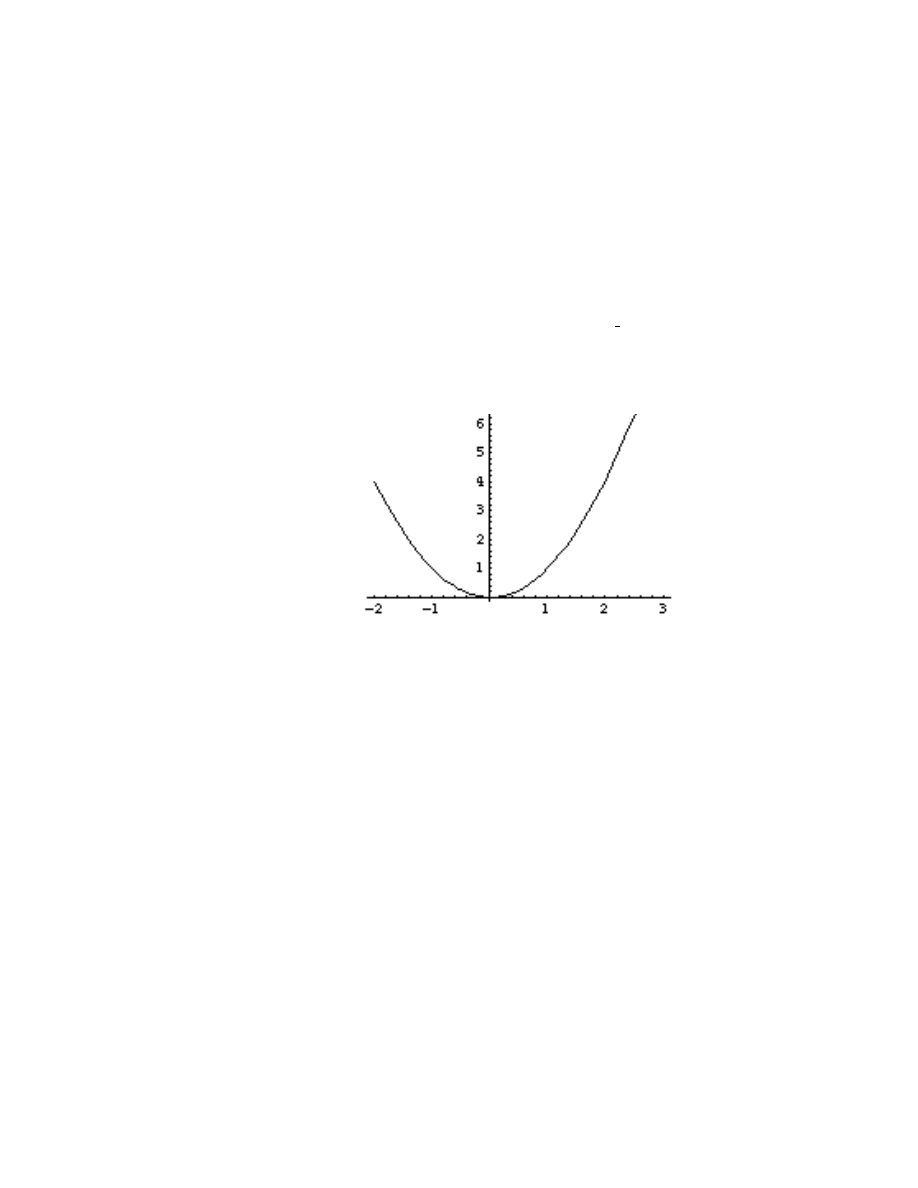
Elementary graphing in Mathematica is handled by the Plot[ ] function. If expr is an expression
with x as its only variable, to create a graph of the equation y=expr as x goes from a to b, use
the command Plot[expr,
{x,a,b}]. To create a graph of the parabola y=x
2
as x goes from -2 to
3, you could enter Plot[xˆ2,
{x,-2,3}]. Or you could formally define f[x ]:= xˆ2 first, and then use
Plot[f[x],
{x,-2,3}]. Or you could define f as the expression x
2
by using f=x
2
and then entering
Plot[f,
{x,-2,3}]. All of these commands should generate the graphic
Plot[ ] has a lot of options which will allow you to control exactly what the graph looks like.
Using the basic Plot[ ] function allows Mathematica to use what it thinks is the best choice for
these options.
You can create a plot of more than one function on the same set of axes by using lists. If you
wished to plot the graphs of y=x, y=
x
2
, and y=sin(3x) on the same set of axes (say as x goes from
-3 to 3), you would use the command Plot[
{x,xˆ2,Sin[3x]},{x,-3,3}].
There’s also no reason why x has to be the variable - Plot[ tˆ2,
{t,-2,3}] will generate exactly
the same plot of a parabola as we did above.
Section Two - Plot Options
There are about 30 options for the Plot[ ] command which allow you to customize the way
plots are generated. The options for Plot[ ] follow the following notation:
Plot[f[x],
{x,a,b}, option1->Value1,option2->Value2,...]. You may enter or omit as many options as
you want. A complete list of the options for the Plot[ ] command and their default values can be
34
seen by evaluating the command Options[Plot]. Rather than describe every possible option, here
is a list of how the most common ones are used.
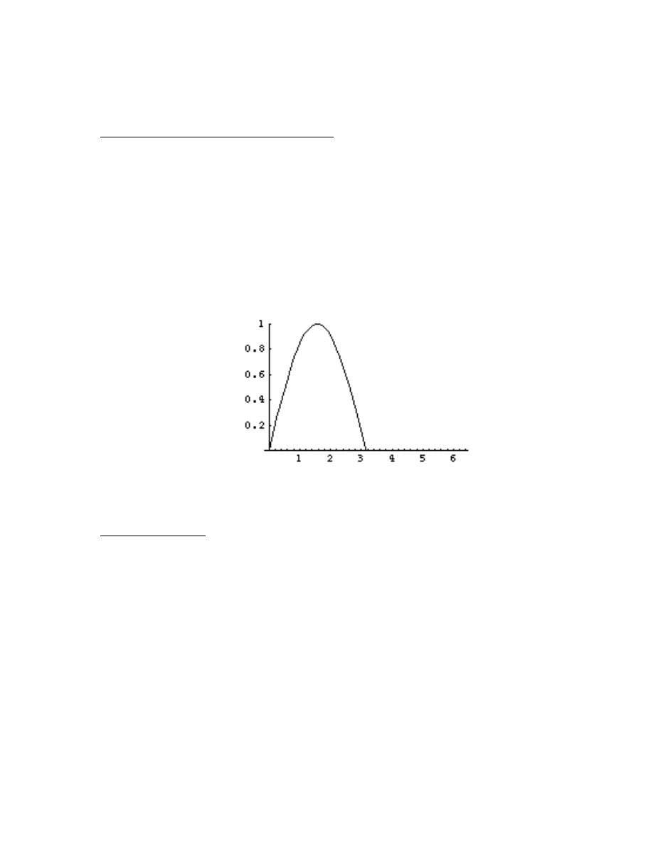
Controlling the range of y-values in the graph: The option PlotRange controls which y-values
will be shown.
For example, if you want to show the y-values from 2 to 6, use the option
PlotRange-
>
{2,6}. This option is important for “zooming” in on certain features of the graph.
For example, if a graph has a vertical asymptote (like tan(x) and 1/x do), Mathematica may try
to plot very large ranges for y, say y going from -1000 to 1000. This scale will make it impossible
to see any local details on the graph. The graph may have a local maximum at (2,3), but you’ll
never see it on that scale. Restricting the range of y-values will allow you to see more features
of the graph. An example of this option would be Plot[Sin[x],
{x,0,2Pi},PlotRange->{0,1}], which
generates the graphic
You can also force Mathematica to try to plot all y-values that occur in a graph (sometimes a
graph might be “beheaded” by the edges of the plot) - to do this, use PlotRange-
>All.
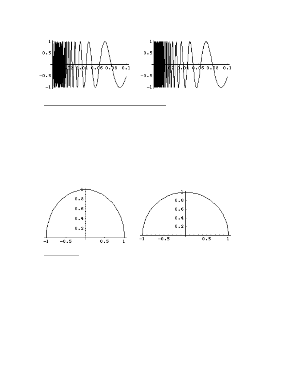
Plotting more points: The option PlotPoints controls how many points are plotted in the
graph. Mathematica creates graph by plotting a lot of points and then trying to connect them
cleverly. The number of points it uses is PlotPoints. The default value is 25. If a graph has very
rapid changes in it (like y=sin(1/x) does near x=0) or the range of x-values is large, 25 points
may not be enough to capture the true behavior of the graph. Using more points by using the
option PlotPoints-
>50 or PlotPoints->100 may make the picture a bit better. An example would
be Plot[Sin[1/x],
{x,-.2,.2},PlotPoints->100]. Of course, the more points you plot the longer it takes
to graph and the more memory Mathematica may need. Below are two graphs - one of sin(1/x)
with no PlotPoints specified (on the left) and one with PlotPoints-
>100 (on the right). Notice how
much more even the graph on the right is - even though the curve goes wild as x gets close to 0 in
both pictures, the oscillations seem much more even in the second graph.
35
Controlling the relative height and width of the graph: AspectRatio is the ratio of height to
width of the graph. Mathematica creates plots which are roughly 3/5 as tall as they are wide,
primarily for aesthetic reasons. To do this, it may use a different scale on the x-axis than the
y-axis. This will distort the graph somewhat - circles may appear as ellipses, for example. Setting
AspectRatio-
>Automatic will create plots with the same scale on both axes, preserving the shapes
of graphs. Setting AspectRatio-
>1 will create a plot as tall as it is wide. The following graphic is
two shots of the top half of the unit circle - on the left using the default value of AspectRatio, on
the right with AspectRatio-
>Automatic.
Removing Axes: If you do not want axes in your graph (if they obscure an important part of
the graph, perhaps), you can remove them with the Axes option by setting Axes-
>None.
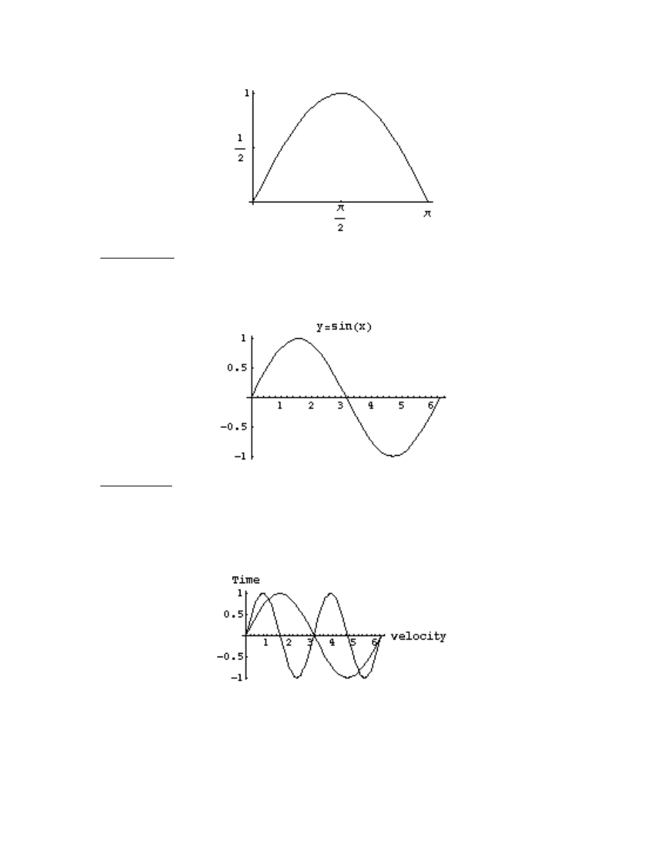
Tick Marks on Axes: The tick marks on the axes are controlled by the option Ticks. Setting
Ticks-
>None will remove all tick marks on the axes. If list1 is a list of what x-ticks you want
and list2 is a list of the y-ticks you want, setting Ticks-
>
{list1,list2} will force Mathematica to use
these tick marks and no others. The Table[ ] and Range[ ] commands are useful for generating the
lists for the tick marks. Some examples are Plot[Sin[x],
{x,0,Pi},Ticks->{{0,Pi/2,Pi},{0,1/2,1}}]
and Plot[xˆ2,
{x,-3,3},Ticks->{Table[i,{i,-3,3}], Table[j,{j,0,9}]}]. The plot of the sine curve in this
example is
36
Labeling Plots: The option PlotLabel allows you to put a label on plots. The label you
use should have double quotes around it; PlotLabel-
>“y=sin(x)”, for example. A full example is
Plot[Sin[x],
{x,0,2Pi},PlotLabel->“y=sin(x)”].
Labeling Axes: AxesLabel places labels on the axes. The option AxesLabel-
>
{“xlabel”,“ylabel”}
labels the x-axis with xlabel and the y-axis with y-label. An example is Plot[
{Sin[x],Sin[2x]},{x,0,2Pi},
AxesLabel-
>
{“velocity”,“time”}]. Just as for PlotLabel, the labels must be surrounded by double-
quote marks.
You can combine these options in a single graph - for example, you can use the command
Plot[Sin[x],
{x,0,2Pi},PlotRange->{-3/2,3/2},AxesLabel->{“x”,“y”}, PlotLabel->“y=sin(x)”,
AspectRatio-
>Automatic, Ticks->
{Table[ i Pi/4,{i,0,8}],{-3/2,-1,-1/2,0,1/2,1,3/2}}].
37
You may not need to know to use an option like AspectRatio until after you’ve done an initial
plot. You can always go back and edit and then reevaluate the cell, of course. You can also use
the Show[ ] command which allows you to replot with different options. For example, suppose you
wanted to plot the top half of a circle of radius two with the command Plot[Sqrt[4-xˆ2],
{x,-2,2}].
The plot will look somewhat elliptical because Mathematica is using different scales in the x- and y-
directions. You can immediately replot by using the command Show[%,AspectRatio-
>Automatic]
as the next command after the original plot. You can alter as many of these options at once as you
want (except for PlotPoints) by using Show[ ].
You can assign nicknames to plots just like you can numbers and functions. You could enter
f=Plot[Sqrt[4-xˆ2],
{x,-2,2}] and then use Show[f,AspectRatio->Automatic], for example.
Show[ ] can be used to plot multiple curves on the same set of axes as well. If you let
f=Plot[Sqrt[4-xˆ2],
{x,-2,2}] and g=Plot[Sin[x],{x,-2,2}], then Show[f,g] will combine the plots into
a single graph.
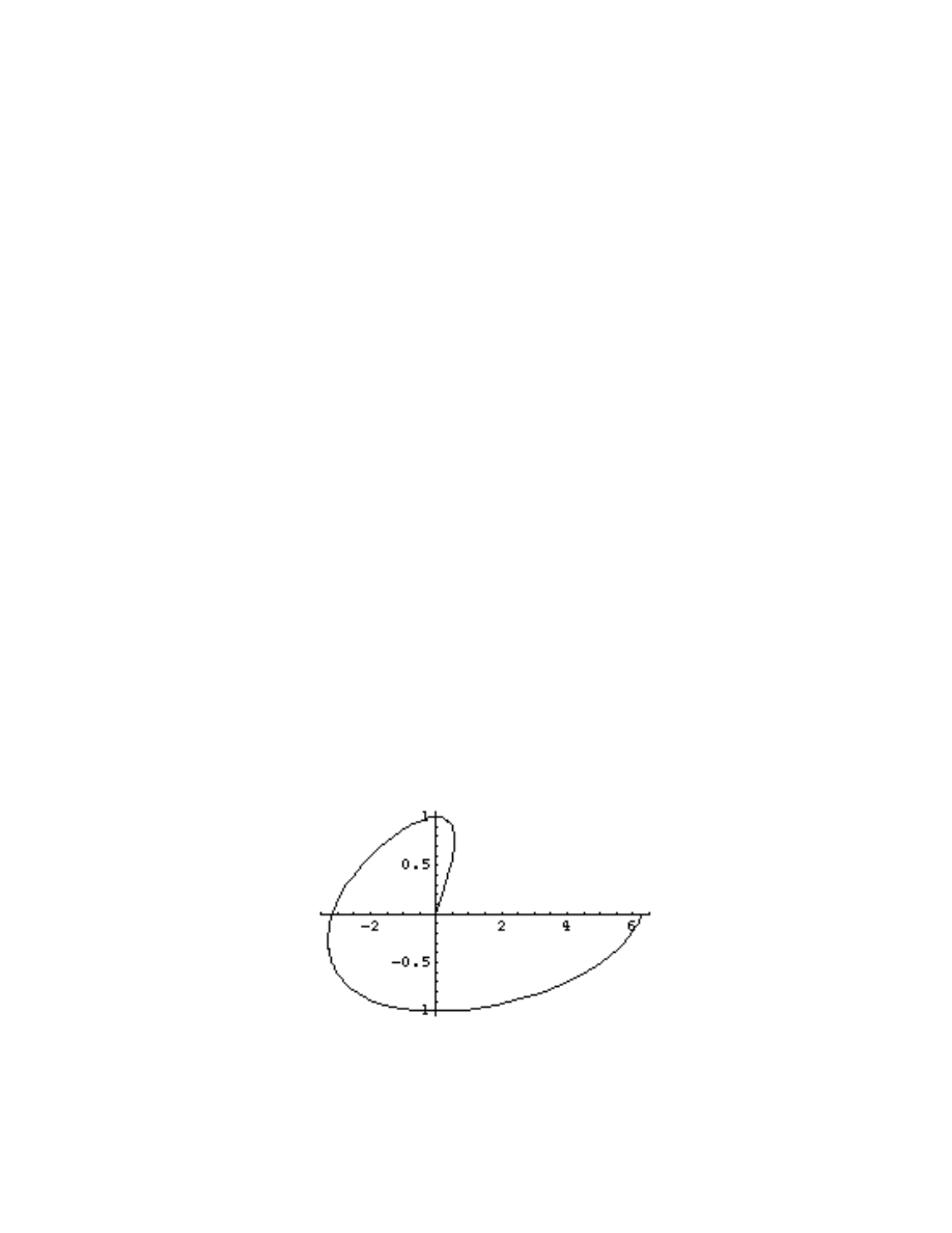
Section Three - Parametric Plots
Mathematica can generate plots parametrically using the command ParametricPlot[ ]. If the
x-coordinate of a point is given by f(t) and the y-coordinate is given by g(t), then the parametric
plot from t=a to t=b is generated by ParametricPlot[
{f[t],g[t]},{t,a,b}]. For example, to plot the
curve defined by x=t*cos(t) and y=sin(t) as t goes from t=0 to 2
π, use the command
ParametricPlot[
{t Cos[t],Sin[t]},{t,0,2Pi}]. This parametric plot should look like this:
The options for ParametricPlot[ ] are the same as for Plot[ ] and entered in exactly the same
fashion (including the use of Show[ ] to change options or combine plots). For example, you could
enter the command:
38
ParametricPlot[
{t Cos[t],Sin[t]},{t,0,2Pi}, AspectRatio->Automatic, AxesLabel->{“x”,“y”}].
One common type of parametric plot is the the graph of a curve in polar coordinates. Such
curves can be graphed using ParametricPlot[ ] and the formulas for translating x and y in terms of
r and
θ or by using a special command PolarPlot[ ] which can be loaded in from the
Graphics`Graphics`package.
Section Four - Plotting the Graphs of Equations
The unit circle is given by
x
2
+
y
2
= 1. You cannot plot this as the graph of a single function
- the best you can do is to solve for y as
±
√
1
− x
2
and then use Plot[
{Sqrt[1-xˆ2],-Sqrt[1-xˆ2]},
{x,-1,1}]. You can plot the graph of the equation x
2
+
y
2
= 1 directly using the command
ImplicitPlot[ ]. Unlike Plot[ ], ImplicitPlot[ ] resides in one of the add-on packages, so you must
first load the package by evaluating
<<Graphics`ImplicitPlot`. Once you have done this, you can
then use the ImplicitPlot[ ] command as follows. Let eqn by an equation like xˆ2+yˆ2==1. To
plot the graph of the equation as x goes from a to b, use the command ImplicitPlot[eqn,
{x,a,b}].
For example, to plot the unit circle above you would enter ImplicitPlot[xˆ2+yˆ2==1,
{x,-1,1}] (you
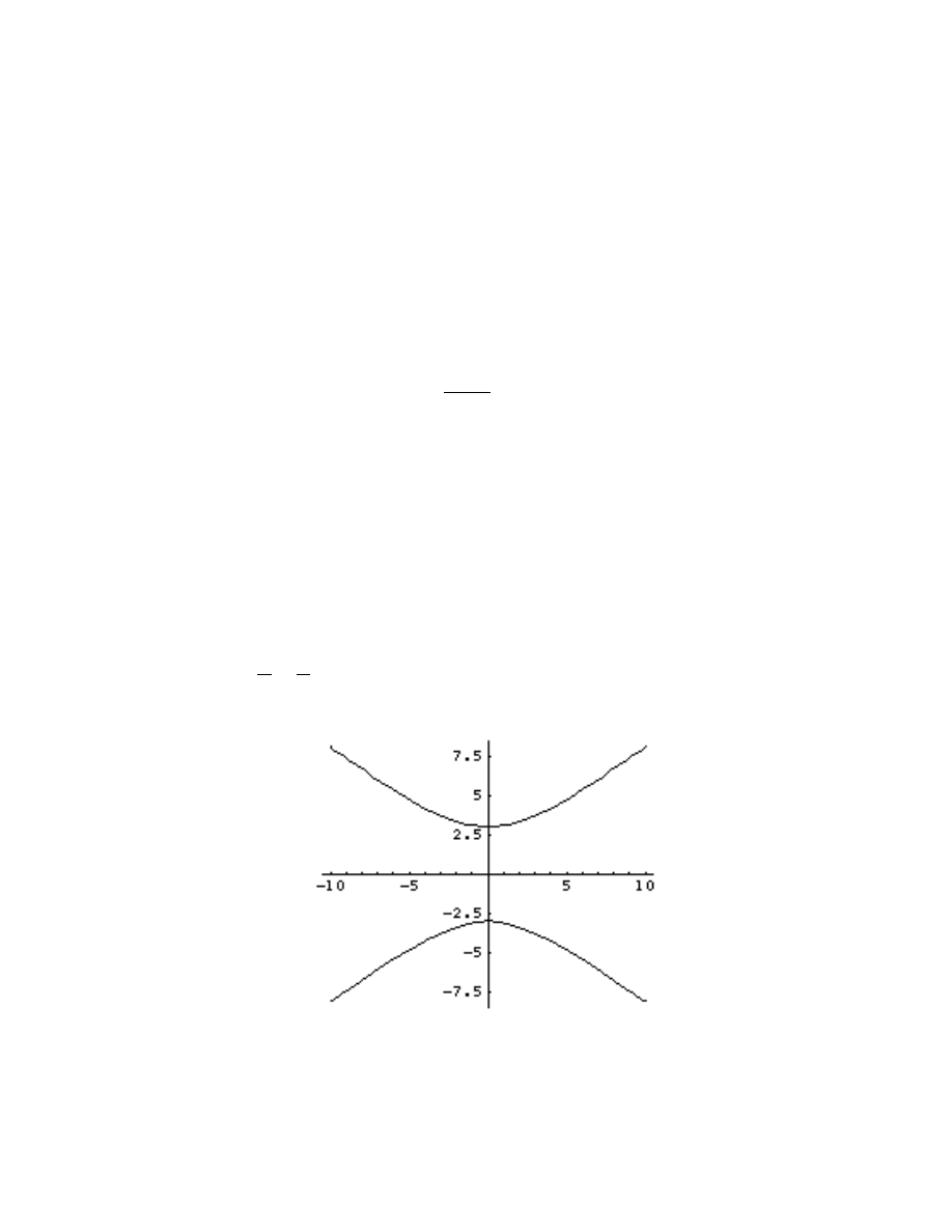
could plot it from x=-2 to 2, but this would just include some empty space around the circle). To
plot the hyperbola
y
2
9
−
x
2
16
= 1 as x goes from -10 to 10, you would use the command
ImplicitPlot[yˆ2/9-xˆ2/16==1,
{x,-10,10}]. This hyperbola should look like:
ImplicitPlot[ ] uses the same options as Plot[ ] does (AspectRatio, AxesLabel, and so on).

39
Chapter Eight Exercises
1) Graph
y = x
3
as x goes from -2 to 3.
2) Graph y=sin(x) and cos(2x) on the same set of axes as x goes from 0 to 10
π.
3) Graph y=cos(x) from 0 to 2
π. Use tick marks 0,
π
2
, π,
3
π
2
, 2π on the x-axis and 0,
1
2
, 1 on the
y-axis. Label the plot “y=cos(x)”.
4) Plot y=
1
x
3
−x
from x=-5 to 5. Restrict the range of y-values displayed to -5 to 5.
5) Create a plot of y=
√
9
− x
2
as x goes from -3 to 3. Use AspectRatio-
>Automatic and label
both axes.
6) Create a plot of the parametric curve defined by x=t cos(t), y=t sin(t) as t goes from 0 to
10. Use AspectRatio-
>Automatic, and have Mathematica sample the functions 50 times to create
the plot.
7) Create a plot of the curve defined by x=sin(2t), y=sin(t) as t goes from 0 to 20.
8) Create a graph of the ellipse
x
2
9
+
y
2
4
= 1 as x goes from -4 to 4. Preserve the shape of the
graph.
9) Create an plot of the curve
y
2
=
x
3
− 16x as x goes from -20 to 20. Label the axes of the
plot.
10) Plot the solution to the initial value problem
y
0
= 2
y
− y
2
, y(0) =
1
2
as x goes from 0 to 5,
showing y-values from 0 to 3.
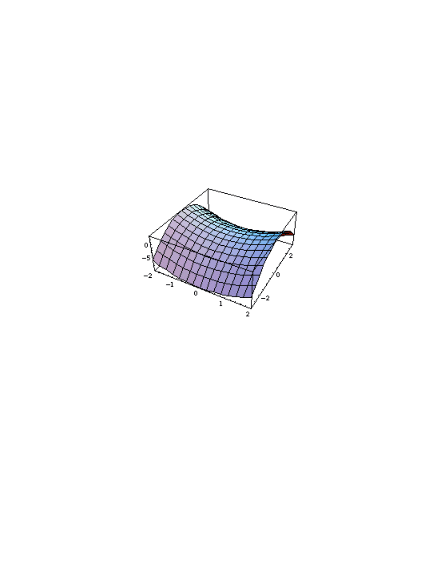
40
Chapter Nine - Three-Dimensional Plots
Section One - Basic 3-D Plots
The command for creating three-dimensional plots is Plot3D[ ]. To create a plot of the surface
z=f(x,y) over the rectangle consisting of x-values from x=a to x=b and y-values from y=a to y=b,
use the command Plot3D[f[x,y],
{x,a,b},{y,a,b}]. For example, to create a plot of the hyperbolic
paraboloid z=
x
2
− y
2
as x goes from -2 to 2 and y goes from -3 to 3, you would enter the command
Plot3D[xˆ2-yˆ2,
{x,-2,2},{y,-3,3}]. You should see the following graphic:
The format for Plot3D[ ] is exactly the same as for the Plot[ ] command, except you have to add
the second list for the variable y and its range. Another way to plot this function would to first
define f=xˆ2-yˆ2, and then enter Plot3D[f,
{x,-2,2},{y,-3,3}]. This approach would be useful if you
are going to work with
x
2
− y
2
- taking derivatives, plugging in numbers with the /. notation, and
so on.
Unlike the Plot[ ] command, you cannot use Plot3D[ ] to plot more than one surface in the same
3-dimensional box. You can, however, combine 3-dimensional plots using the Show[ ] command,
just as you can for plots.
For example, define a= Plot3D[xˆ2-yˆ2,
{x,-2,2},{y,-3,3}] (the paraboloid above) and define
b=Plot3D[-xˆ2,
{x,-3,3},{y,-3,3}] (the graph of this is a cylindrical surface generated by a parabola
which opens downward). If you then evaluate Show[a,b], you will create a 3-dimensional plot of
the two surfaces in the same space. You could achieve the same effect using the % notation - just
follow the two 3-D plot commands with Show[%,%%].
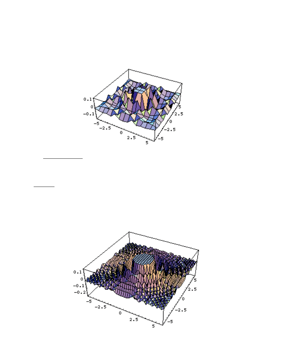
41
Section Two - Plot3D[ ] options
In the following, define f=Sin[xˆ2+yˆ2]/(xˆ2+yˆ2). Evaluate Plot3D[f,
{x,-6,6},{y,-6,6}] - you
should see the graphic below. There are several flaws in this graphic which will illustrate some of
the important options for Plot3D[ ].
The plot is jagged: The plot is very jagged, filled with sharp edges and corners. This is
because like it does in Plot[ ], Mathematica creates 3-D plots by plotting a bunch of points and
then connecting the values (this time with polygons rather than line segments). The function
sin
(
x
2
+
y
2
)
x
2
+
y
2
changes very rapidly away from the origin, so Mathematica is not using enough points
to get a good idea of what the surface looks like. We can increase the number of points Mathematica
samples using the option PlotPoints, just as for Plot[ ]. If you enter Plot3D[f,
{x,-6,6},{y,-6,6},
PlotPoints-
>40], this will replot the surface much more smoothly, and you will be able to see the
“ripples” in the surface around the origin. This plot is given below.
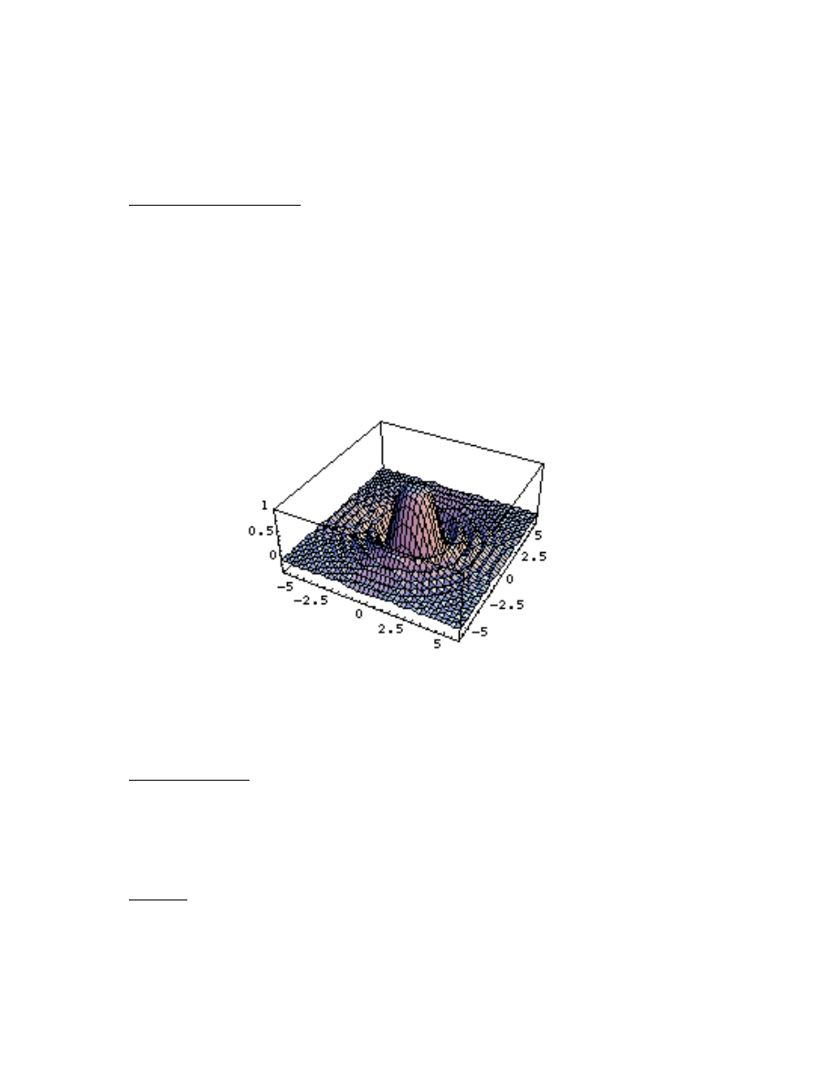
42
When increasing PlotPoints, keep in mind than the work it takes to create the surfaces goes
up as the -square- of the number of points being sampled. If you go from PlotPoints-
>20 to
PlotPoints-
>40, it will take roughly four times as much time and memory to create the plot.
Not all z-values are shown: Even if you increase the number of points being plotted (as in the
plot above), you will notice that the part of the surface over the origin is “beheaded” - it is not
shown and the result looks completely flat. Mathematica has its own rules for what it considers
“optimal” ranges of z-values to plot. You can override this with the PlotRange option.
PlotRange-
>
{zmin,zmax} will tell Mathematica to cut the surface off outside of the z-range
zmin -zmax, and PlotRange-
>All will force it to try to plot the range of all z-values in the sur-
face. If you evaluate Plot3D[f,
{x,-6,6},{y,-6,6},PlotPoints->40,PlotRange->All], you will see why
Mathematica cut the original surface off. This plot is:
There is one large spike over the origin, which dwarfs the smaller ripples in the surface to the
point where they are not easy to make out. A similar effect can be created by viewing the z-values
from -1 to 1 with the command Plot3D[f,
{x,-6,6},{y,-6,6},PlotPoints->40,PlotRange->{-1,1}].
The bounding box: In all of the Plot3D[ ] commands above, Mathematica draws a box around
the plot. You can remove this box with the option Boxed-
>False. This will not remove the axes
on the edges, just the other edges of the box. For an example, enter the command
Plot3D[f,
{x,-6,6},{y,-6,6},PlotPoints->40,Boxed->False].
The axes: Axes are drawn in the edges of the bounding box so they are not hidden behind
the surface. There are two options which deal with the axes themselves. If you wish to remove
the axes (that is, not have the axes distinguished from the other edges of the bounding box), use
the option Axes-
>False. Unless you combine this with the Boxed->False option, the lines will still
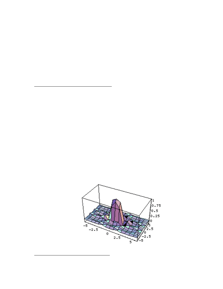
43
be drawn without tick marks. To add labels to the axes, use the command AxesLabel-
>
{xlabel
,ylabel ,zlabel
}. Just as for Plot[ ], the labels you use should be enclosed in double-quote marks.
For example, to remove the bounding box and tell which axis is which in the previous plot evaluate
Plot3D[f,
{x,-6,6},{y,-6,6},PlotPoints->40,PlotRange->All, Boxed->False,
AxesLabel-
>
{“x-axis”,“y-axis”,“z-axis”}]. The graphic this produces may be very compressed - to
make it larger, first click on the graphic and then left-click on the lower right corner and drag to
change the size.
Changing the relative dimensions of the plot: Mathematica tries to preserve the scales on the
x-axis ,y-axis, and z-axis when possible. But you may want to override its decisions. For example,
you may want a plot which is 3 times as tall as normal, or one where the y-direction is twice as long
as the x-direction. You can do this with the option BoxRatios. BoxRatios-
>
{a,b,c} creates a plot
whose relative dimensions are a in the x-direction, b in the y-direction, and c in the z-direction.
Using BoxRatios-
>
{1,1,3} creates a plot whose length in the z-direction is 3 times that of the x-
and y- directions. Using BoxRatios-
>
{1,2,3} creates a plot whose length in the y-direction is twice
that in the x-direction and whose length in the z-direction is three times than of the length in the
x-direction. BoxRatios is literally a set of ratios - using BoxRatios-
>
{1,2,1} will yield exactly the
same results as using BoxRatios-
>
{2,4,2} will, since the ratios x-to-z, y-to-z, and x-to-z are the
same in each option. The following picture is the result of evaluating the command
Plot3D[f,
{x,-6,6},{y,-6,6},PlotRange->All,BoxRatios ->{2,1,1}]. Notice how the scales at the base
of the graph have been distorted - the x-axis is now twice as large as the y-axis.
The viewpoint you look at the surface from: In all of the 3-D plots generated so far, the van-
tage you view the surface from is the same - you are viewing the surface from a point which is
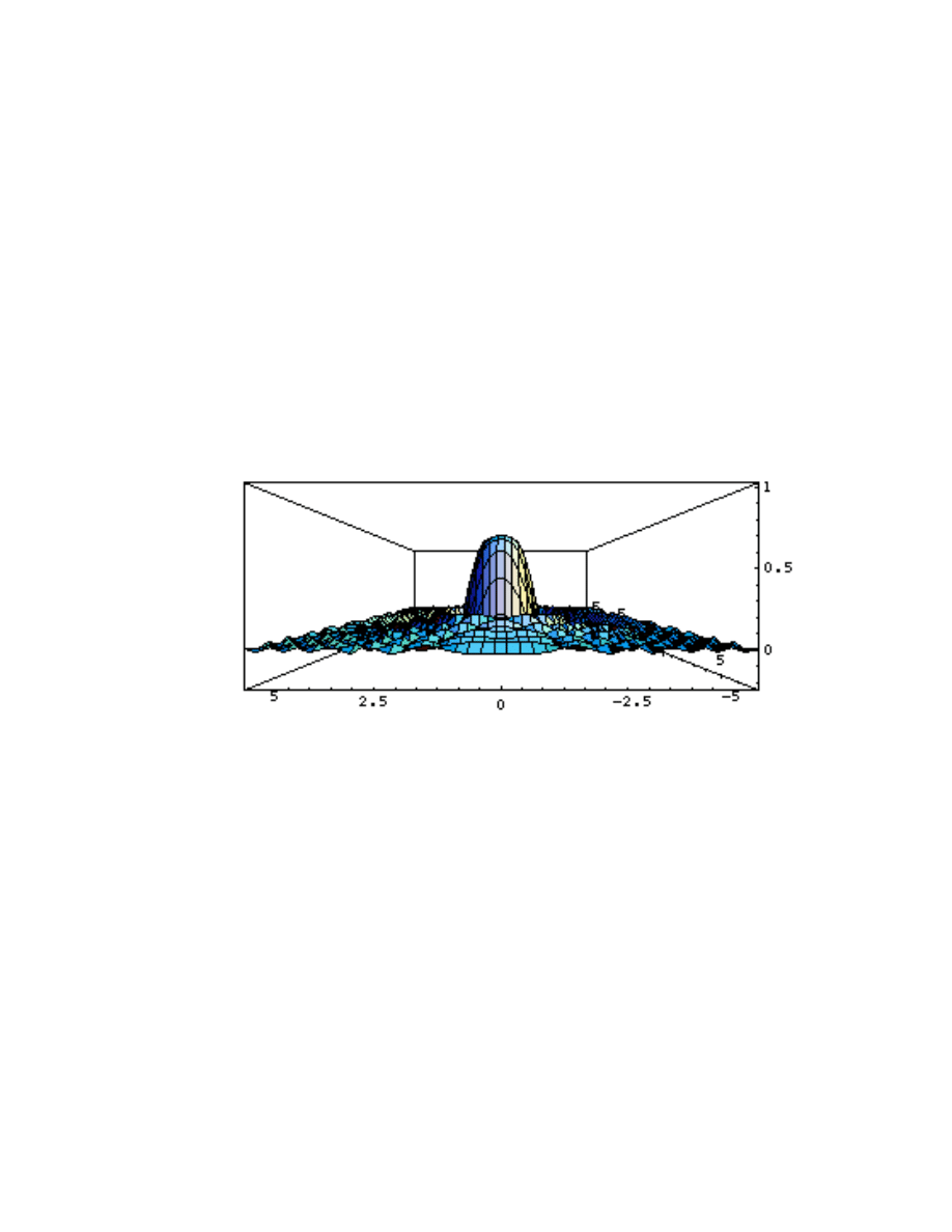
44
above the fourth quadrant of the xy-plane (this is much easier to figure out if you label the axes
using AxesLabel). You may want to view the surface from other points - from directly below or
above, for example. You can control the vantage point using the option ViewPoint. If you use
the option ViewPoint-
>
{a,b,c}, you will view the surface from a point on the ray starting at the
origin (0,0,0) through the point (a,b,c). For example, to view the surface from up on the z-axis,
set ViewPoint-
>
{0,0,1}. To view it from underneath, set ViewPoint->{0,0,-1}. If you wish to view
the surface from above the 1st quadrant in the xy-plane, try ViewPoint-
>
{1,1,1}. The following
graphic is generated using ViewPoint-
>
{0,1,0} - we’re looking at the surface from somewhere on
the y-axis.
Mathematica has another way to select a viewpoint. Under the Input menu, there is a selection
called 3D Viewpoint Selector. If you select this, a new window will pop up with a cube with labeled
sides. Left-click somewhere on the cube and drag it - this will rotate the cube, giving you a hands-
on way of visualizing viewpoints (this is easier to reconcile with coordinates if the dialog button
“Cartesian” is selected, so it will show you coordinates in the usual way). Once you’ve rotated the
cube so you see it from a vantage point you think will be useful, click the “Paste” button. This will
insert the appropriate ViewPoint-
>
{whatever} directly into your document at the point where the
cursor was - the only thing it won’t do for you is put in the appropriate comma. If you wanted to
use the viewpoint selector for the surface we’ve defined by f, you would enter the partial command
Plot3D[f,
{x,-6,6},{y,-6,6},|], leaving the cursor where the | is. (don’t actually type the |). Go into
the viewpoint selector, drag the cube, and hit “Paste”. The cell is now ready to evaluate and when
you evaluate it you will get the view you wanted.
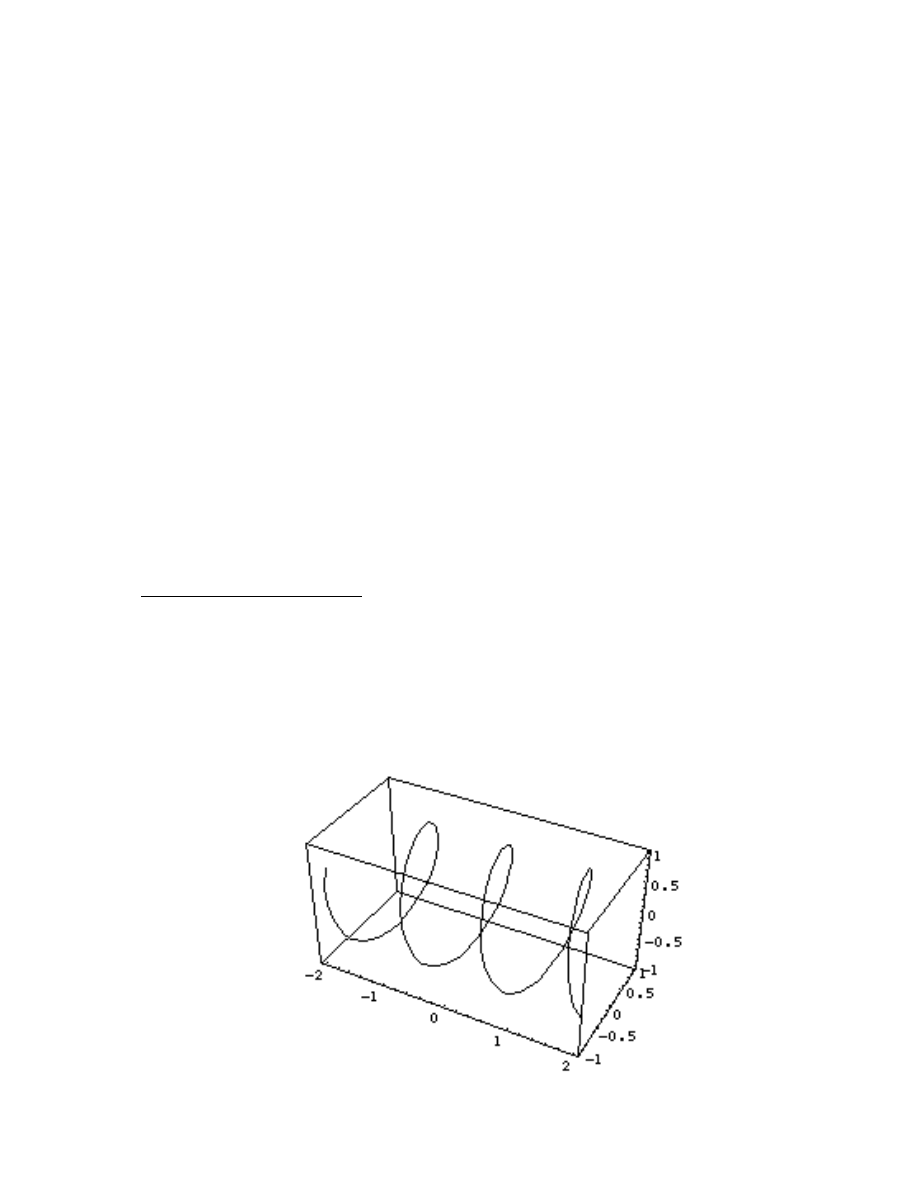
45
There are many other options for Plot3D[ ] which control other aspects of the plot like how
the surfaces are colored and how lights are placed around the surface to produce shadows. You
can get a complete listing of these options and their default values by evaluating the command
Options[Plot3D].
The Show[ ] command can be used to alter options in a 3-D plot the same was as for the Plot[ ]
command. For example, you could first evaluate Plot3D[f,
{x,-6,6},{y,-6,6}], then Show[%,
PlotRange-
>All], then Show[%,Boxed->False,AxesLabel->
{“x-axis”,“y-axis”, “z-axis”}].
Section Three - Parametric 3D Plots
Mathematica can also do parametric plot in 3-space. Unlike parametric plots in the plane,
there are two different types of parametric plots you can do. You can parametrically plot a curve
(where the x-, y-, and z-coordinates all depend on a single variable, say t ), or a surface (where the
x-, y-, and z-coordinates of points are functions of a pair of variables, say u and v). Both types of
parametric plots are done with the same command - ParametricPlot3D[ ].
Plotting Parameterized Curves: To a plot a curve whose coordinate functions are x=f(t),
y=g(t), and z=h(t) over the t-interval tmin-tmax , use the command
ParametricPlot3D[
{f[t],g[t],h[t]},{t,tmin , tmax }]. For example, to create a plot of the helix defined
by x=y/5, y=cos(t), and z=sin(t) as t goes from -10 to 10, you would use the following command:
ParametricPlot3D[
{t/5,Cos[t],Sin[t]},{t,-10,10}]. This curve is shown below:
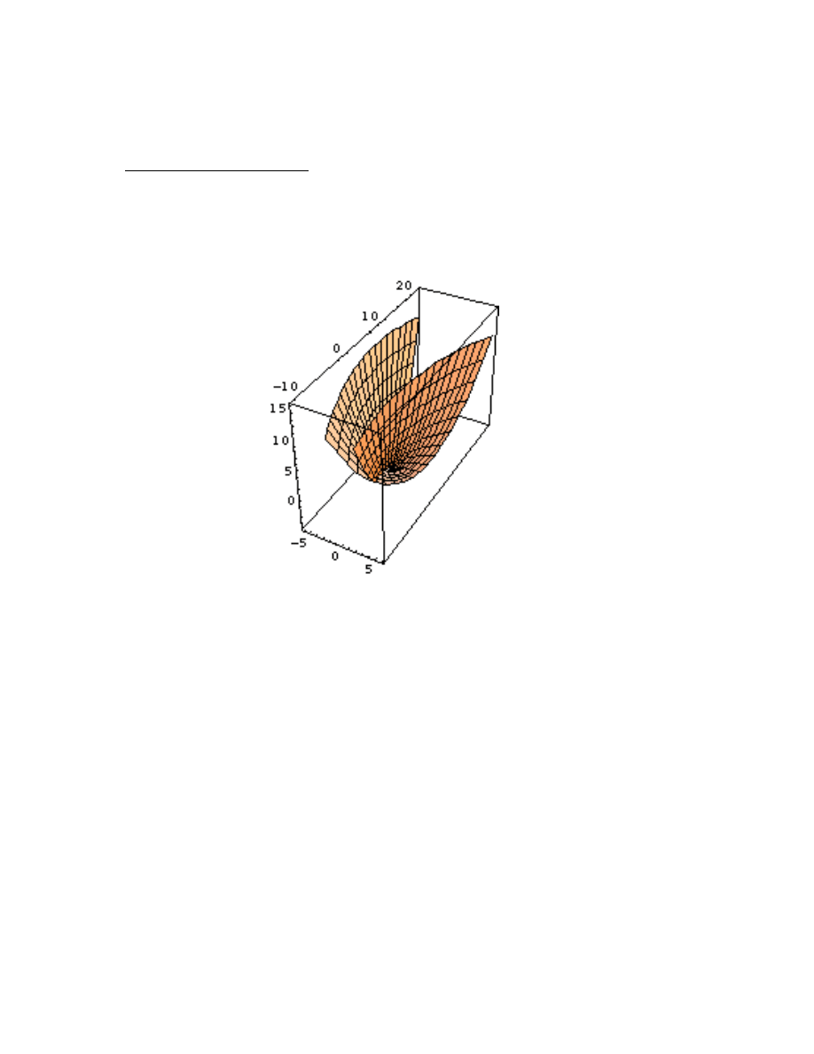
46
There is nothing special about using t for the variable in a curve defined using parameters -
it’s just a common usage.
Plotting Parametric Surfaces: Plotting surfaces is very similar to plotting parameterized curves.
To plot the surface whose coordinates are given by x=u+v, y=u
2
-uv, z=v
2
-u
2
for values of u be-
tween -2 and to and values of v from -4 to 4, you would use the command
ParametricPlot3D[
{u+v,uˆ2-u v, vˆ2-uˆ2},{u,-2,2},{v,-4,4}]. This particular surface looks like:
Again, there nothing special about the use of the u and v as the independent variables - it’s
just a common convention.
Plotting surfaces defined by parameterizations takes a lot of horsepower, so you may have to
wait a few moments for the entire plot to be generated. If this is the case, you will see the phrase
“Rendering” appear in the title bar of the Mathematica window.
ParametricPlot3D[ ] uses many of the same options as Plot3D[ ] - Boxed, Axes, AxesLabel,
BoxRatios, and especially PlotPoints and ViewPoint. Surfaces defined using parameters often
change their height very rapidly, so it is fairly common to use the PlotPoints option to get a smoother
picture of the surface (remember, as you increase the value of PlotPoints, it takes more time for
the computer to get the plot). These types of surfaces and curves often wrap around themselves
and sometimes intersect themselves, so it is usually a good idea to construct several different plots
with different ViewPoint values so you can see underneath and around the surfaces/curves - and

47
you can used Axes-
>False and Boxed->False to remove axes and bounding boxes of they get
in the way.

48
Chapter Nine Exercises
1) Plot
z = x
3
− y
3
as x and y go from -3 to 3.
2) Replot the function from problem 1 but restrict the z-values displayed to the range -4 to 6.
3) Create a plot of
z = x
2
− y
2
as x and y go from -3 to 3 with no bounding box whose scale
in the z direction is 5 times larger than that of the x- and y- directions.
4) Create a plot of
z = sin(e
xy
) as x and y go from -2 to 2. Make Mathematica sample enough
points to get a relatively smooth picture of the surface, and label the axes of the plot.
5) Create a plot of the curve defined by x=sin(t), y=cos(t), z=sin(
√
2t) as t goes from 0 to
10
π. Label the axes and make Mathematica sample enough points to get a smooth curve.
6) Create a plot of the surface defined by
x =
sin(
u)
√
v
, y = cos(2u), z = v as u goes from 0 to 2π
and v goes from 1 to 9.

49
Solutions to Exercises
The answers to the exercises are given as a Mathematica command or sequence of commands.
If a problem takes more than one command, “followed by” or “and” indicate the sequence of
commands. If a problem involves defining a function or nickname, it would probably be a good
idea to use Clear[ ] to remove the definitions before going on to the next exercise.
Chapter One Exercises
1) N[PiˆE] followed by N[EˆPi] and see which is bigger.
2) Evaluate Iˆ2, Iˆ3, Iˆ4, Iˆ5, and Iˆ6.
3) N[E,15]
4)
<<Graphics`ImplicitPlot`followed by <<Graphics`Polyhedra`
5)
<<Algebra`ThisIsNotARealPackage`
This will give you an error message.
Chapter Two Exercises
1) (256ˆ2-8128)/40
2) Sqrt[964]
3) Abs[(2ˆ4-3ˆ3)/(6ˆ7-7ˆ6)]
4) Evaluate 20!
5) Binomial[20,4]
6) N[Sin[1]] followed by N[Sin[90]]. The latter is not 1 because the 90 is 90 radians, not degrees.
7) Cos[I Log[2]]
8) ArcCos[1/2] followed by N[ArcSin[3/5]]
9) Tan[ArcSin[1/7]] followed by N[%]
10) N[Log[3]] followed by N[Log[10,3]]
11) N[Sinh[1]] followed by N[Cosh[1]]
12) f[x ]:=Sin[x]/(Cos[x]+3)
13) g[x ]:= xˆ(1/Log[x]) (g[2] and g[3] will both return E).
14) h[x ,y ]:=xˆ2-sin(x y) followed by h[0,3]
15) ?f followed by ?g followed by ?h
16) Clear[f] followed by Clear[g] followed by Clear[h]

50
17) The k[x ] expression defines a function you can evaluate at values like k[3] or k[t+1], but k=3x-4
defines k as a nickname for 3x-4.
18) x=3 defines x as a nickname for 3, but x==3 is a True/False test for whether the variable x is
equal to 3.
19) MyCubeRoot[x ]:= Sign[x] Abs[x]ˆ(1/3)
Chapter Three Exercises
1) Range[30] or Table[i,
{i,1,30}]
2) Table[2i+1,
{i,0,29}]
3) a=
{1,2,-3,x,5,y} followed by a[[3]] and a[[6]]
4) Table[2ˆi,
{-10,20,5}]
5)
{{1,1/2,1/3,1/4,1/5},{2,1,2/3,1/2,2/5},{3,3/2,1,3/4, 3/5},{4,2,4/3,1,4/5}}
6) a=Table[i/j,
{i,1,4},{j,1,5}] followed by Length[a] and Dimensions[a]
7) Union[
{1,2,3,1,2}]
8) Intersection[Table[4i,
{i,1,100}],Table[5j,{j,1,75}]]
9) a=
{{1,3,1},{2,4,1},{3,6,2}} followed by MatrixForm[a]
10) f=3xˆ5-15x+5 followed by f/. x-
>1, f/.x->2, and f/.x->3
11) Sin[x y]-xˆ2 y /.
{x->Pi/4,y->2}
12) xˆ4-xˆ3 /. Table[
{x->i},{i,-1,5}]
13) xˆ2+2x y-yˆ2-6x+4y+1 /.
{x->x1+h, y->y1+k}
Chapter Four Exercises
1) Simplify[ ( (x+h)ˆ4-xˆ4)/h] followed by %/.
{h->0}
2) f=Expand[ xˆ2+2x y-yˆ2-6x+4y+1 /.
{x->x1+h, y->y1+k}] followed by Coefficient[f, x1 y1]
followed by Coefficient[f,x1] and Coefficient[f,y1]. Notice that the x1 coefficient involves y1 and vice
versa. The coefficient of just the first degree term x1 can be obtained by Coefficient[f,x1]/.
{y1->0}
and the coefficient of the first degree term y1 can be obtained by Coefficient[f,y1]/.
{x1->0}
3) Apart[xˆ12/(xˆ8-1)] followed by Together[%]
4) Factor[xˆ20-1]
5) FactorInteger[2ˆ126-1]

51
6) PolynomialDivision[xˆ6-xˆ4+7,xˆ3-1,x]
7) Cancel[(xˆ12-1)/(xˆ9-1)]
8) Simplify[(x+2)ˆ3-(x-1)ˆ2+(x+9)ˆ4-1]
Chapter Five Exercises
1) Solve[
{3x+2y==1,6x-y==10},{x,y}]
2) Solve[
{3x+2y==1,6x+4y==5},{x,y}]
3) Solve[
{3x+2y==1, 9x+6y==3},{x,y}]
4) Solve[
{3x+3y-z==1,x-3y+2z==0,x-4y-z==-3},{x,y,z}]
5) Solve[
{xˆ2+yˆ2==4,y==3x+1},{x,y}]
6) Solve[xˆ2+2x-6==0,x]
7) Solve[xˆ2+4x+10==0,x]
8) Solve[xˆ3-4x+1==0,x]
9) Solve[xˆ4+3xˆ2-6x+2==0,x]
10) NSolve[xˆ4+3xˆ2-6x+2==0,x]
11) NSolve[3xˆ5-15x-5==0,x]
12) Solve[x==10Log[x],x] followed by N[%]
13) xˆ2-1 /. Solve[xˆ3-xˆ2-4x+4==0,x]
Chapter Six Exercises
1) Limit[Sin[x]/x,x-
>Pi], Limit[Sin[x]/x,x->0], and Limit[Sin[x]/x,x->Infinity]
2) Limit[(3xˆ2-3x+2)/(6xˆ5-5x-1),x-
>Infinity]
3) Limit[2ˆx/(xˆ3+1),x-
>Infinity]
4) D[xˆ3-6xˆ2-2x+1,x]
5) D[xˆ2 Exp[x],x,x] or D[xˆ2 Exp[x],
{x,2}]
6) Simplify[D[xˆ(1/Log[x]),x]]
7) D[Exp[xˆ2],
{x,4}] /. x->1
8) x/. Solve[ D[xˆ4-4xˆ3+2xˆ2-9,x]==0,x]
9) f=(xˆ2 y-yˆ2)/(xˆ2+yˆ2) followed by D[f,x], D[f,y], D[f,x,x], D[f,y,y], and D[f,x,y].

52
10) Normal[ Series[Tan[x],
{x,0,3}]] followed by Normal[ Series[Tan[x],{x,0,5}]] followed by Normal[
Series[Tan[x],
{x,0,10}]] followed by %%% /. x->1/2 followed by %%% /. x->1/2 followed by %%%
/. x-
>1/2
11) Integrate[xˆ2 Sin[x],x]
12) Integrate[1/(xˆ3-1),x]
13) Integrate[ Sum[xˆn/nˆ2,
{n,2,Infinity}],x]
14) Integrate[xˆ3 Exp[x],
{x,0,1}]
15) Integrate[xˆ2/Exp[x],
{x,1,Infinity}]
16) N[Sum[(n+1)/nˆ4,
{n,2,Infinity}] ]
17) DSolve[ y
0000
[x]-y[x]==0,y[x],x]
18) DSolve[
{y
00
[x]+y[x]==0,y[0]==3,y’[0]==2
},y[x],x]
19) DSolve[
{y
00
[x]-y[x]==0,y’[0]==3,y’[0]==2
},y[x],x]
20) DSolve[
{y
000
[x]+y[x]==Sin[x],y[0]==0,y’[0]==1,y
00
[0]==1
},y[x],x]
21) f= (y[x]/.DSolve[
{y
00
[x]+y[x]==0,y[0]==3,y’[0]==2
},y[x],x])[[1]]
The y[x]/. command tells Mathematica to replace y[x] with the solution from DSolve[ ] - but
this is a list, so the [[1]] at the end returns the first (and only) element of the list.
Chapter Seven Exercises
1)
{1,0,3}.{2,-1,3}
2)
{3,4,1,4}.{-2,1,0,3}
For 3-8, define a=
{{1,2,3},{4,5,6},{2,1,5}} and b={{3,2,1},{0,-6,5},{1,2,3}}. To view the results
as matrices, put the commands inside a MatrixForm[ ] command.
3) a-b
4) 2a+b
5) a.b-b.a
6) Transpose[a]
7) Det[a]
8) Inverse[a]
9) Define c=
{{1,2,1},{2,6,1},{1,1,0}}, then evaluate Eigenvalues[c] and Eigenvectors[c]

53
Chapter Eight Exercises
1) Plot[xˆ3,
{x,-2,3}]
2) Plot[
{Sin[x],Cos[2x]},{x,0,10Pi}]
3) Plot[Cos[x],
{x,0,2Pi},Ticks->{{0,Pi/2,Pi,3Pi/2,2Pi},{0,1/2,1} },PlotLabel->“y=cos(x)”]
4) Plot[1/(xˆ3-x),
{x,-5,5},PlotRange->{-5,5}]
5) Plot[Sqrt[9-xˆ2],
{x,-3,3},AspectRatio->Automatic, AxesLabel->{“x-axis”,“y-axis”}]
6) ParametricPlot[
{t Cos[t], t Sin[t]},{t,0,10},AspectRatio->Automatic, PlotPoints->50]
7) ParametricPlot[
{Sin[2t],Sin[t]},{t,0,20}]
8) After loading in the ImplicitPlot package (see solutions to Chapter One Exercises), use
ImplicitPlot[xˆ2/9+yˆ2/4==1,
{x,-4,4}]. Or you could solve for y and use
Plot[
{2Sqrt[1-xˆ2/9],-2Sqrt[1-xˆ2/9]},{x,-4,4}] (this will cause Mathematica to give some errors,
but it should still plot).
9) Load the ImplicitPlot Package and use ImplicitPlot[yˆ2==xˆ3-16x,
{x,-20,20},
AxesLabel-
>
{ “x-axis”,“y-axis”}]
10) Define f by f=(y[x]/.DSolve[
{y’[x]==2y[x]-y[x]ˆ2,y[0]==1/2},y[x],x ])[[1]], and then use
Plot[f,
{x,0,5},PlotRange->{0,3}]
Chapter Nine Exercises
1) Plot3D[xˆ3-yˆ3,
{x,-3,3},{y,-3,3}]
2) Show[%,PlotRange-
>
{-4,6}]
3) Plot3D[xˆ2-yˆ2,
{x,-3,3},{y,-3,3},Boxed->False, BoxRatios->{1,1,5}]
4) Plot3D[Sin[Exp[x y]],
{x,-2,2},{y,-2,2},PlotPoints->50,AxesLabel->{“x-axis”,“y-axis”,“z-axis”}]
5) ParametricPlot3D[
{Sin[t],Cos[t],Sin[Sqrt[2]t]},{t,0,10Pi},PlotPoints->50]
6) ParametricPlot3D[
{Sin[u]/Sqrt[v],Cos[2u],v},{u,0,2Pi},{v,1,9}]
Wyszukiwarka
Podobne podstrony:
Brief Introduction to Hatha Yoga
Heathen Gods and Rites A brief introduction to our ways of worship and main deities
A brief Introduction to Database Theory ver1 4
Dahl M A brief introduction to Finsler geometry (web draft, 2006)(39s) MDdg (1)
Introduction to the Runes brief background information on runes, with table of Elder Futhark rune m
Machamer; A Brief Historical Introduction to the Philosophy of Science
Introduction to VHDL
268257 Introduction to Computer Systems Worksheet 1 Answer sheet Unit 2
Introduction To Scholastic Ontology
Evans L C Introduction To Stochastic Differential Equations
Zizek, Slavoj Looking Awry An Introduction to Jacques Lacan through Popular Culture
Introduction to Lagrangian and Hamiltonian Mechanics BRIZARD, A J
Introduction to Lean for Poland
An Introduction to the Kabalah
Introduction to Apoptosis
więcej podobnych podstron