13

Boundary Mesh Free Methods

The boundary element method (BEM) is a numerical technique based on the boundary
integral equation (BIE), which has been developed since the 1960s. For many problems,
BEM is undoubtedly superior to the “domain discretization” types of methods, such as
the finite element method (FEM) and the finite difference method (FDM). BEM has a well-
known advantage of dimension reduction for linear problems. For example, only the two-
dimensional (2D) bounding surface of a three-dimensional (3D) body needs to be dis-
cretized. BEM is applicable to all the problems for which the fundamental solution (Green’s
functions) is known in a reasonably simple form, preferably in a closed form.

The mesh free idea has also been used in BIE, such as the boundary node method (BNM)

(Mukherjee and Mukherjee, 1997a; Kothnur et al., 1999; Chati et al., 1999; Chati and
Mukherjee, 2000) and the local boundary integral equation (LBIE) method (Zhu and Atluri,
1998). These boundary type mesh free methods are formulated using the moving least
squares (MLS) approximations and approaches and techniques of BIE. In BNM, the surface
of problem domain is discretized (presented to be exact) by properly scattered nodes. The
BNM has been applied to 3D problems of both potential theory and the theory of elasto-
statics (Chati et al., 1999; Chati and Mukherjee, 2000). Very good results have been obtained
in these problems. However, because the shape functions based on MLS interpolants lack
the delta function property, extra efforts are needed to satisfy the boundary condition
accurately in BNM. This problem becomes even more serious in BNM because of the large
number of boundary conditions, compared with the total number of nodes for the problem.
The method used by Kothnur et al. (1999) to impose boundary conditions resulted in a
set of system equations that are doubled in number. The advantage of the boundary-type
method is therefore eroded and discounted to a certain degree, making BNM computa-
tionally much more expensive than conventional BEM.

G. R. Liu and Gu (2001a,e) have developed a boundary-type MFree method called the

boundary point interpolation method (BPIM), where the point interpolation method (PIM)
proposed by G. R. Liu and Gu (1999; 2001c) is used to construct shape functions. It is
confirmed that there is no need at all to use MLS in boundary-type MFree methods,
especially for 2D problems. PIM works much more efficiently in constructing shape func-
tions, and all the PIM shape functions possess the Kronecker delta function property. This
removes the issue of treatment of boundary conditions, which is especially beneficial to
methods based on BIE. The dimension of the equation system of BPIM is equivalent to
that of BEM. For 2D problems, BPIM works perfectly well without any special trick and
is superior to BNM in simplicity, accuracy, and computational efficiency. For 3D problems
for which 2D shape functions need to be constructed, there could be an issue of singular
moment matrices. In such cases, the special techniques discussed in Section 5.5.5 should
be applied.

An effective way of constructing PIM shape functions is to use radial functions as the

basis. The advantage of using a radial function basis is that it guarantees the existence of

1238_Frame_C13.fm Page 545 Wednesday, June 12, 2002 5:27 PM

© 2003 by CRC Press LLC

the inverse moment matrix (see Section 5.7). The methods formulated and coded by Gu and
Liu (2001a) are termed boundary radial PIM (BRPIM).

This chapter focuses on the introduction of boundary MFree methods formulated using

both MLS shape functions (BNM) and PIM shape functions (BPIM and BRPIM). These
boundary MFree methods can be formulated in the same manner, except that in formu-
lating BNM using MLS shape functions proper treatment of essential boundary conditions
(see Mukherjee and Mukherjee, 1997b; Kothnur et al., 1999) is required.

Only 2D problems are discussed in this chapter. In all these boundary MFree methods,

only the boundary of the problem domain is represented by properly scattered nodes. BIE
for 2D elastostatics is then discretized using MFree shape functions based only on a group
of arbitrarily distributed boundary nodes that are included in the support domain of a
point of interest.

For 3D BNM, readers are referred to the work by Chati et al. (1999).

13.1 BPIM Using Polynomial Basis

A BPIM using polynomial basis in the construction of shape functions is first presented
in this chapter for solving boundary value problems of solid mechanics. The method was
originally proposed by Gu and Liu (2001e). The PIM shape functions are constructed in
a curvilinear coordinate system, and possess the delta function property. The boundary
conditions can be implemented with ease as in conventional BEM. In addition, the rigid
body movement can also be utilized to avoid some singular integrals. For 2D problems,
BPIM with polynomial basis will have no singularity problem of interpolation as we have
seen in the domain type of PIMs, as the boundaries are curves, and the interpolation is
basically one dimensional. Therefore, there is no reason to use MLS approximations in
this case.

Detailed formulation of BPIM using polynomial basis is presented, and several numer-

ical examples are presented to demonstrate the validity and efficiency of BPIM. A com-
parison study is carried out using BPIM, BNM that uses MLS shape functions,
conventional BEM, and analytical methods.

13.1.1

Point Interpolation on Curves

Consider a 2D domain

Ω

bounded by its boundary

Γ

, as shown in

Figure 13.1.

In using

boundary MFree methods, only the boundary

Γ

of the problem domain is represented

using nodes. The point interpolants in BPIM are constructed on the 1D bounding curve

Γ

of 2D domain

Ω

, using a set of discrete nodes on

Γ

. As in the conventional BEM

formulation, the displacement and traction can be constructed independently using PIM
shape functions. The displacement

u

(

s

) and traction

t

(

s

) at a point

s

on the boundary

Γ

is

expressed using the surrounding nodes and polynomials:

(13.1)

(13.2)

u s

( )

p

i

s

( )a

i

i=1

n

∑

p

T

s

( )a

=

=

t s

( )

p

i

s

( )b

i

i=1

n

∑

p

T

s

( )b

=

=

1238_Frame_C13.fm Page 546 Wednesday, June 12, 2002 5:27 PM

© 2003 by CRC Press LLC

where

s

is a curvilinear coordinate (the arc-length for a 2D problem) on

Γ

,

n

is the number

of nodes in the support domain of a point of interest at

s

Q

,

which is often a quadrature

point of integration,

p

i

(

s

) is a basis function of a complete polynomial with

p

1

=

1 and

p

i

=

s

i

−

1

, and

a

i

and

b

i

are the coefficients that change when

s

Q

changes. In matrix form, we

have

a

T

=

[

a

1

,

a

2

,

a

3

,

,

a

n

]

(13.3)

b

T

=

[

b

1

,

b

2

,

b

3

,

,

b

n

]

(13.4)

p

T

(

s

)

=

[

1,

s

,

s

2

,

s

3

,

s

4

,

,

s

n

−

1

]

(13.5)

The coefficients

a

i

and

b

i

in Equation 13.1 can be determined by enforcing Equation 13.1

to be satisfied at the

n

nodes surrounding the point

s

Q

. Equation 13.1 can then be written

in the following matrix form:

u

n

=

P

Q

a

(13.6)

t

n

=

P

Q

b

(13.7)

where

u

n

and

t

n

are the vectors of nodal displacement and traction, given by

u

n

=

[

u

1

,

u

2

,

u

3

,…,

u

n

]

T

(13.8)

t

n

=

[

t

1

,

t

2

,

t

3

,…,

t

n

]

T

(13.9)

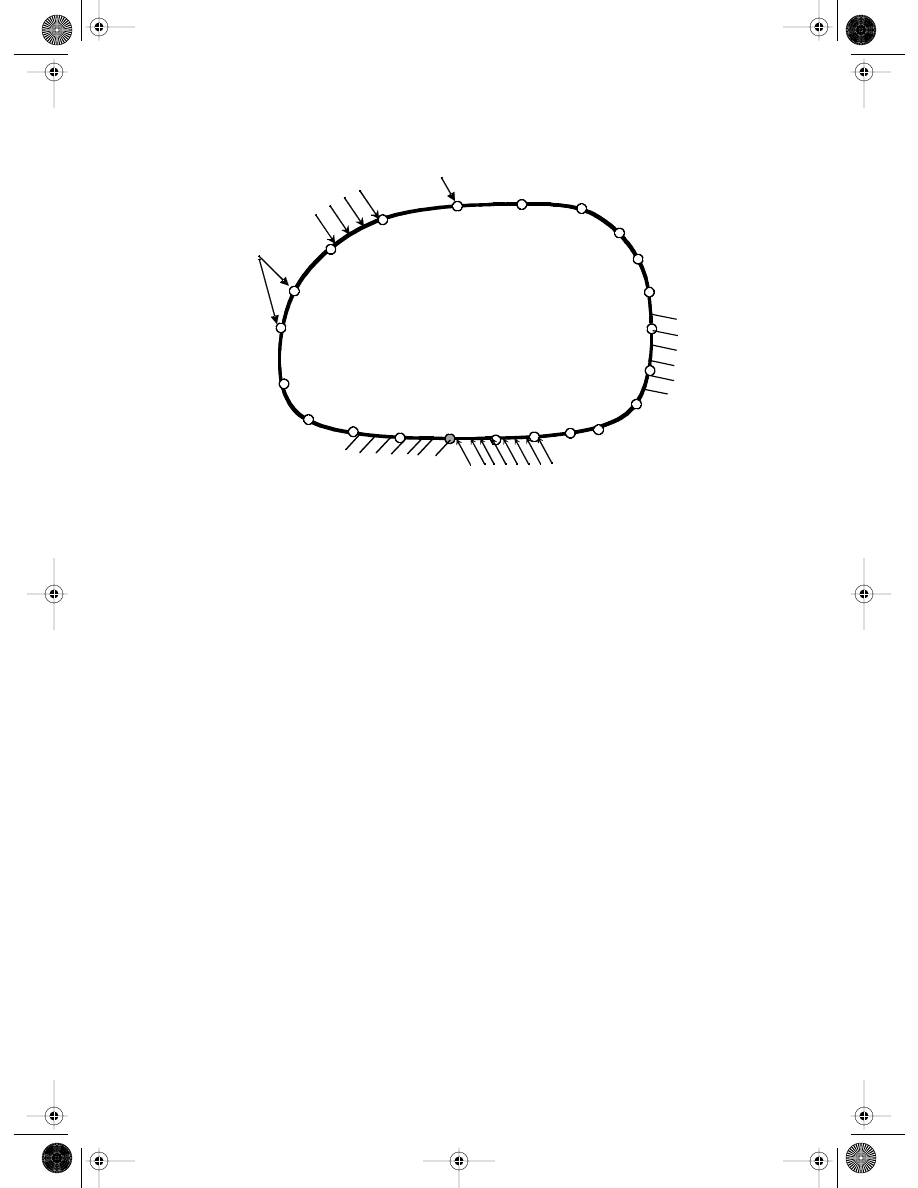
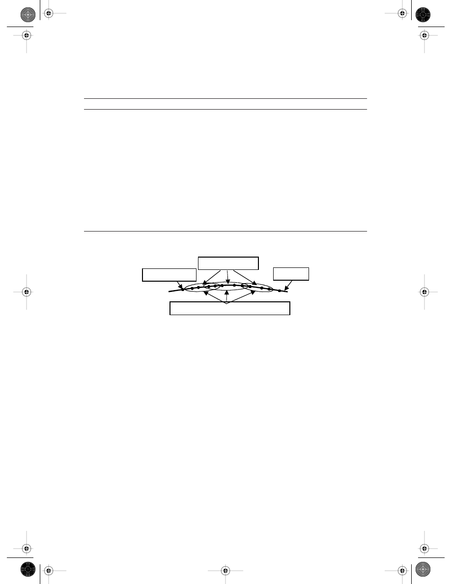
FIGURE 13.1

Domains and their boundaries: problem domain

Ω

boundary bounded by its boundaries

Γ

including essential

(displacement) boundary

Γ

u

, natural (force or free) boundary

Γ

t

. In boundary MFree methods, only the problem

boundary is represented using nodes.

Γ

u

Γ

t

Ω

Γ

Nodes

Nodes i

Γ

t

Γ

t

Γ

u

…

…

…

1238_Frame_C13.fm Page 547 Wednesday, June 12, 2002 5:27 PM

© 2003 by CRC Press LLC

and

P

Q

is the moment matrix formed by

(13.10)

Solving a and b from Equations 13.6 and 13.7, and then substituting them into Equation
13.1, we obtain

u

(s) = Φ

Φ

Φ

Φ

T

(s)u

n

(13.11)

t

(s) = Φ

Φ

Φ

Φ

T

(s)t

n

(13.12)

where the matrix of shape function

Φ

Φ

Φ

Φ(s) is defined by

Φ

Φ

Φ

Φ

T

(s) = p

T

(s)

=

[

φ

1

(s),

φ

2

(s),

φ

3

(s), ,

φ

n

(s)]

(13.13)

The shape function

φ

i

(s) obtained from above procedure satisfies

φ

i

(s = s

i

)

= 1 i = 1, n

(13.14)

φ

j

(s = s

i

)

= 0 j ≠ i

(13.15)

(13.16)

Therefore, the interpolation functions constructed have the delta function property, and
the boundary conditions can be easily imposed as in traditional BEM. The procedure to
prove these properties can be found in

Chapter 5.

The matrix P

Q

is an n

× n matrix. It needs to be invertible for the construction of the

shape functions in Equation 13.13. Fortunately, in the curvilinear coordinate system, the
matrix P

Q

is, in general, reversible for the 2D problem (interpolation along a 1D boundary).

It can be found that the accuracy of interpolation depends on the nodes in the support

domain of a quadrature point. Therefore, a suitable support domain should be chosen to
ensure a proper area of coverage for interpolation. To define the support domain for a
point s

Q

, a curvilinear support domain is used. The arc-length of the curvilinear domain

d

s

is computed by

d

s

=

α

s

d

c

(13.17)

where

α

s

is the dimensionless size of the support domain and d

c

is a characteristic length

that relates to the nodal spacing near the point at s

Q

. If the nodes are uniformly distributed,

d

c

is the distance between two neighboring nodes. In the case where the nodes are non-

uniformly distributed, d

c

can be defined as an “average” nodal spacing in the support

domain of s

Q

. The procedure of determining d

c

can be performed following the procedure

in Section 2.10.3 for the 1D case based on our current curvilinear coordinate system.

As discussed in Section 5.11, the PIM approximation could be incompatible. Similarly

to the domain type in PIM methods, we can also formulate nonconforming and conforming
BPIMs.

In using nonconforming BPIM, the support domain is determined for each and every

Gauss point. In conforming BPIM, however, we use so-called one-piece shape functions
for an integration cell to ensure the compatibility of the field function approximation with
the cells. Therefore, the support domain is defined for the cell, meaning all the Gauss
points in the cell share the same support domain and hence the same PIM shape functions.
The support domain of a cell is determined in a manner similar to that discussed in the

P

Q

T

p

s

1

( ), p s

2

( ), p s

3

( ), …, p s

n

( )

[

]

=

P

Q

1

–

…

φ

i

s

( )

i

=1

n

∑

1

=

1238_Frame_C13.fm Page 548 Wednesday, June 12, 2002 5:27 PM

© 2003 by CRC Press LLC

previous paragraph. The only difference is that the domain is centered at the geometrical
center of the cell and not at the Gauss point.

Note that for boundary type PIMs, because the integration cells are connected at points

(not lines), the compatibility is automatically enforced, as long as the one-piece PIM shape
functions are used. There is no need to use the penalty method to enforce compatibility
as we have done in

Chapter 8

for two-dimensional cases.

The number of nodes, n, can be determined by counting all the nodes in the support

domain. The dimensionless size of support domain

α

s

should be predetermined by the

analyst. We study this in detail using numerical examination to determine the proper
value to use. It must be observed that choosing

α

s

= 2.0 to 3.0 (which includes n

= 3 to 6)

leads to acceptable performance for BPIM.

13.1.2

Discrete Equations of BPIM

The well-known BIE for 2D linear elastostatics, presented by Brebbia (1978), is given by

(13.18)

where c

i

is a coefficient dependent on the geometric shape of the boundary, b is the body

force vector, and u

∗

and t

∗

are the fundamental solution for linear elastostatics. The funda-

mental solution (Brebbia et al., 1984) for a 2D plane strain problem can be used and it is
given by

(13.19)

(13.20)

where G is the shear modulus,

ν is the Poisson’s ratio, ∆ is the Kronecker delta function,

r is the distance between the source point and the field point, n is the normal to the
boundary, and a comma designates a partial derivative with respect to the indicated spatial
variable.

Substituting Equations 13.11 and 13.12 into Equation 13.18 yields the BPIM system

equation for all the nodes on the boundary of the problem domain.

HU

= GT + D

(13.21)

where

(13.22)

(13.23)

(13.24)

c

i

u

i

ut

∗

d

Γ

Γ

∫

+

tu

∗

d

Γ

Γ

∫

=

bu

∗

d

Ω

Ω

∫

+

u

ij

∗

1

8

πG 1 ν

–

(

)

----------------------------

3 4

ν

–

(

) 1

r

---

∆

ij

r

,i

r

, j

+

ln













=

t

ij

∗

1

–

4

π 1 ν

–

(

)r

--------------------------

r

∂

n

∂

-------

1 2

ν

–

(

)∆

ij

r

,i

r

, j

+

[

]

1 2

ν

–

(

) r

,i

n

, j

r

, j

n

,i

–

(

)

–













=

H

c

i

t

∗

Φ

Φ

Φ

Φ

T

d

Γ

Γ

∫

+

=

G

u

∗

Φ

Φ

Φ

Φ

T

d

Γ

Γ

∫

=

D

bu

∗

d

Ω

Ω

∫

=

1238_Frame_C13.fm Page 549 Wednesday, June 12, 2002 5:27 PM

© 2003 by CRC Press LLC

13.1.3

Implementation Issues in BPIM

Singular Integral
To evaluate the integrals given in Equations 13.22 to 13.24, background integration cells
that can be independent of the nodes are required. The cells should be created on the
boundary of the problem domain with proper dimension to ensure an accurate integration.
From Equations 13.19 and 13.20, it can be seen that the integrands in Equations 13.22 to
13.24 consist of regular and singular functions. The regular functions in Equations 13.22
to 13.24 can be evaluated using the usual Gaussian quadrature based on the integration cells.
In Equation 13.23, the matrix G contains a log singular integral. This type of singular
integral can be evaluated by log Gaussian quadrature as follows:

(13.25)

where the required points x

i

and weights w

i

are presented by Brebbia et al. (1984) for

conventional BEMs.

In matrix H defined by Equation 13.22, c is a coefficient dependent on the geometric

shape of the boundary, which is easy to obtain for a smooth boundary. However, it is more
complicated to obtain c for nonsmooth boundaries. In addition, H contains a (1

/r) type

singular integral. Therefore, it can be a nontrivial task to directly evaluate the diagonal
terms of H. The same difficulty has been experienced in conventional BEMs. Note that
shape functions of BPIM possess the delta function property; therefore, the rigid body
movement can be utilized in this work to obtain the diagonal terms of H (Brebbia et al.,
1984).

Application of Boundary Conditions
There are two types of boundary conditions in BPIM

t

=

on the natural boundary

Γ

t

(13.26)

u

=

on the essential boundary

Γ

u

(13.27)

Because the shape functions of BPIM have the delta function property, the boundary

conditions can be imposed in the same way as the traditional BEM. Note that if MLS
shape functions were used, proper treatments are needed (Mukherjee and Mukherjee,
1997b; Kothnur et al., 1999).

After applying the boundary condition, the system (Equation 13.21) has 2N

B

equations

and 2N

B

unknowns for N

B

boundary nodes. The system equation can be solved using

standard routines of an algebraic equation solver to obtain the displacement and traction.

Handling of Corners with Traction Discontinuities
In handling traction discontinuities in corners, special care should be taken. Double nodes
and discontinuous elements at corners are used to overcome this problem in traditional
BEM. Because there are no elements used in BPIM, a simple method proposed by Gu and
Liu (2001e) to solve this difficulty is by displacing the nodes from the corner. The support
domain for interpolation is truncated at the corner. The method is very easy to implement

I

1

/x

(

) f x

( )dx

ln

0

1

∫

=

f x

i

( )w

i

i

=1

m

∑

≅

t

u

1238_Frame_C13.fm Page 550 Wednesday, June 12, 2002 5:27 PM

© 2003 by CRC Press LLC

and is used in the following numerical examples. The simple method is proved to be very
accurate.

13.1.4

Numerical Examples

The BPIM is coded and used to solve a number of problems of mechanics. A detailed com-
parison study is carried out using the present BPIM, BNM, conventional BEM, and analytical
methods. In BNM, a weight function must be used for constructing MLS shape functions.
The exponential weight function (Kothnur et al., 1999) given below is used for the exam-
ples in this section:

(13.28)

where d

i

is the arc-length, d

sQ

is the size of the support of the weight function

, which

is the dimension of the support domain in BNM, and k and c are constants. In this section,
k = 1 and d

sQ

/c = 0.75 are used (Kothnur et al., 1999).

The formulation procedure of BNM is very much similar to that for the nonconforming

BPIM except (1) an MLS shape function is used to replace the PIM shape function; (2)
Lagrange multipliers, or the method proposed by Mukherjee and Mukherjee (1997b), or
any other methods to treat the essential boundary conditions are used.

The following presents some examples analyzed using nonconforming BPIM.

Example 13.1

Cantilever Beam

BPIM is first applied to analyze the displacement and stress field in a cantilever beam,
which is shown in

Figure 6.4.

A plane stress problem is considered. The parameters for

this example are

Young’s modulus for the material: E = 3.0

× 10

7

Poisson’s ratios for two materials:

ν = 0.3

Thickness of the beam: t = 1
Height of the beam: D = 12
Length of the beam: L = 48
Load: P = 1000

The beam is subjected to a parabolic traction at the free end as shown in Figure 6.4. The
analytical solution is available; it can be found in the textbook by Timoshenko and Goodier
(1977) and is listed in Equations 6.28 to 6.33.

A total of 120 uniform boundary nodes are used to discretize the boundary of the beam.

To evaluate the integral of matrices, 120 uniform integration cells are used. The parameter

α

s

in Equation 13.17 for the support domains is fixed at 2.0. Therefore, three to six nodes

are included in the support domain for constructing shape functions.

Figure 13.2

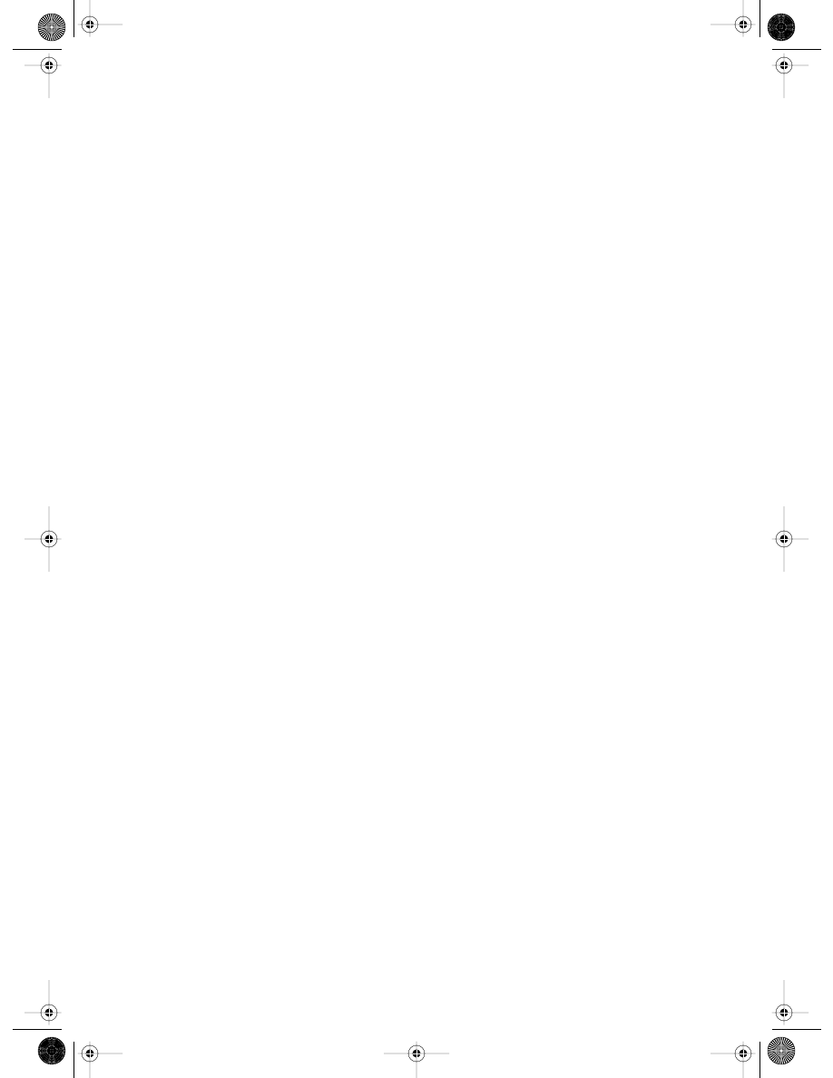
illustrates the comparison between the shear stress calculated analytically

and by BPIM at the section of x = L

/2. The plot shows a good agreement between the

analytical and numerical results. The conventional linear BEM results of this problem are

W

i

s

( )

e

d

i

/c

(

)

–

2k

e

d

sQ

/c

(

)

–

2k

–

1 e

d

sQ

/c

(

)

–

2k

–

------------------------------------------

0

d

d

sQ

≤

d

d

sQ

>











=

)

W

i

)

1238_Frame_C13.fm Page 551 Wednesday, June 12, 2002 5:27 PM

© 2003 by CRC Press LLC

also shown in the same figure for comparison. The density of the nodes in BEM and BPIM
is exactly the same. It is clearly shown that the BPIM results are more accurate than the
BEM results. This is because BPIM uses more nodes for the interpolation of the displace-
ments and tractions. Therefore, the order of the interpolant in BPIM is higher than the
order of the conventional linear elements in BEM.

For the detailed error analysis, we define the following norm as an error indicator using

the shear stress, as the shear stress is much more critical than other stress components in
the cantilever beam to reflect the accuracy.

(13.29)

where N is the number of nodes investigated,

τ is the shear stress obtained numerically,

and is the analytical shear stress.

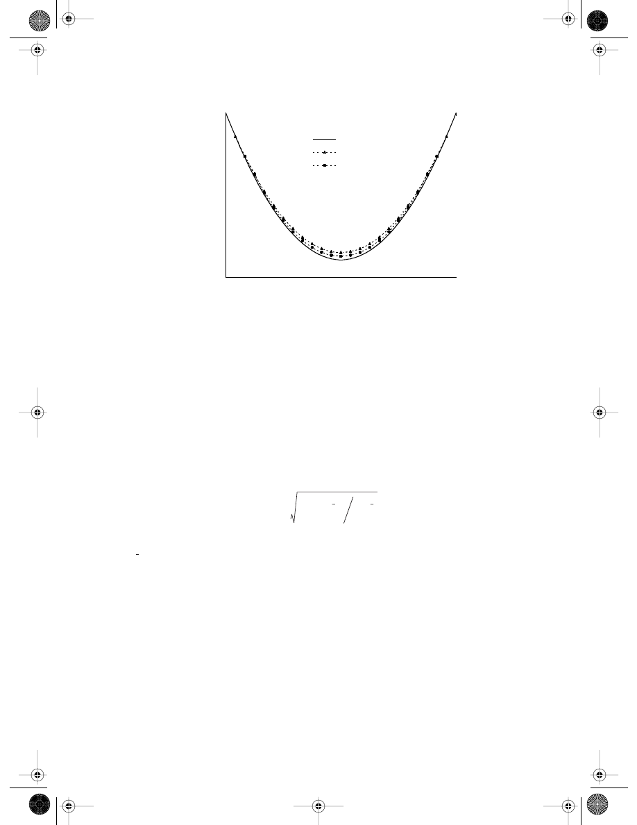
The convergence for the shear stresses at the section of x = L

/2 with mesh refinement is

shown in

Figure 13.3.

The convergences of BNM and conventional linear BEM are also

shown in the same figure, where h is a characteristic length related to the nodal spacing.
Three kinds of nodal arrangement of 40, 240, and 480 uniform boundary nodes are used.
It can be observed that the accuracy of BPIM and BNM using MLS approximation is nearly
the same, but both BPIM and BNM have higher accuracy than BEM. The convergence of
BPIM seems to be the best among these three methods.

As mentioned above, the dimensionless size of support domain

α

s

defined in Equa-

tion 13.17 needs to be chosen such that a “reasonable” number of nodes lie in the support
domain of an evaluation point. The results of e

t

for different sizes of support domain are

shown in

Table 13.1.

In this analysis, the boundary is modeled by 40 uniformly distributed

nodes, and 40 uniformly spaced integration background cells are used. It is found that
the accuracy of the results of BPIM changes slightly with the dimension of the support
domain when the nodal density is fixed. Although the choice of the support domain may

FIGURE 13.2
Shear stress

τ

xy

at the section x

= L/2 of the beam. (From Gu, Y. T. and Liu, G. R., Comput. Mech., 28, 47–54, 2002.

With permission.)

-140.0

-120.0

-100.0

-80.0

-60.0

-40.0

-20.0

0.0

-6

-4

-2

0

2

4

6

y

Shear Stress

Analytical

BEM

BPIM

e

t

1

N

----

τ

i

τ

i

–

(

)

2

i

=1

N

∑

τ

2

i

=1

N

∑

=

τ

1238_Frame_C13.fm Page 552 Wednesday, June 12, 2002 5:27 PM

© 2003 by CRC Press LLC

also depend a little on the type of the problem, it is found that

α

s

= 2.0 to 3.0 works well

for most of the problems investigated in this section.

It may be mentioned here that the use of a large support domain does not necessarily

lead to more accurate results. Similar results were seen for mechanics problems of 2D
solids in

Chapter 8.

Example 13.2

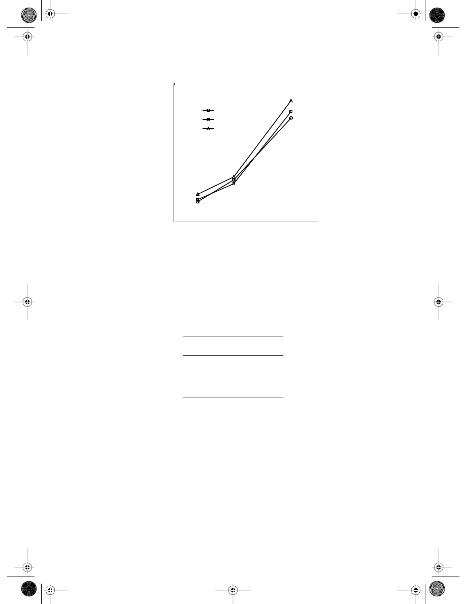
Plate with a Hole

Consider now an infinite plate with a central circular hole subjected to a unidirectional
tensile load of p = 1.0 in the x direction. As a large finite plate can be considered a good
approximation of an infinite plate, a finite square plate of 20

× 20 is considered. Making

use of the symmetry, only the upper right quadrant of the finite plate is modeled as shown
in

Figure 13.4.

Plane strain condition is assumed, and the material properties are E = 1.0

× 10

3

,

ν = 0.3. Symmetry conditions are imposed on the left and bottom edges, and the inner

FIGURE 13.3
Convergence in e

t

norm of error. (From Gu, Y. T. and Liu, G. R., Comput. Mech., 28, 47–54, 2002. With permission.)

TABLE 13.1

The Effects of the Dimension of
the Support Domain on the Error
of Energy Norm

Dimension of
Support Domain (

αααα

s

)

e

t

a

1.0

0.1688

2.0

0.1410

3.0

0.1775

4.0

0.1812

5.0

0.1794

a

Defined by Equation 13.29.

-3.0

-2.5

-2.0

-1.5

-1.0

-0.5

0.0

-0.8

-0.6

-0.4

-0.2

0.0

0.2

0.4

BPIM

BNM

BEM

Log(h)

Log(

e

t

)

1238_Frame_C13.fm Page 553 Wednesday, June 12, 2002 5:27 PM

© 2003 by CRC Press LLC

boundary of the hole is traction free. The tensile load p is imposed on the right edge in
the x direction. The exact solution for the stresses of an infinite plate is given in the textbook
by Timoshenko and Goodier (1977) and is listed in Equations 7.59 to 7.64.

A total of 68 nodes are used to discretize the boundary (with 10 uniformly distributed

nodes on BC, CD, and AE, and 19 nonuniformly distributed nodes along AB and DE).
The same number of integration background cells are used. The support domain of an
evaluation point is determined as in Equation 13.17 (with

α

s

= 2.0, and the characteristic

arc-length: d

Q

= 1.0 on AB, BC, CD, and DE, d

Q

= 0.2 along AE). If the number of nodes

in the support domain is more than six, only six nodes with shorter arc-length to the
integration point are used in the interpolation.

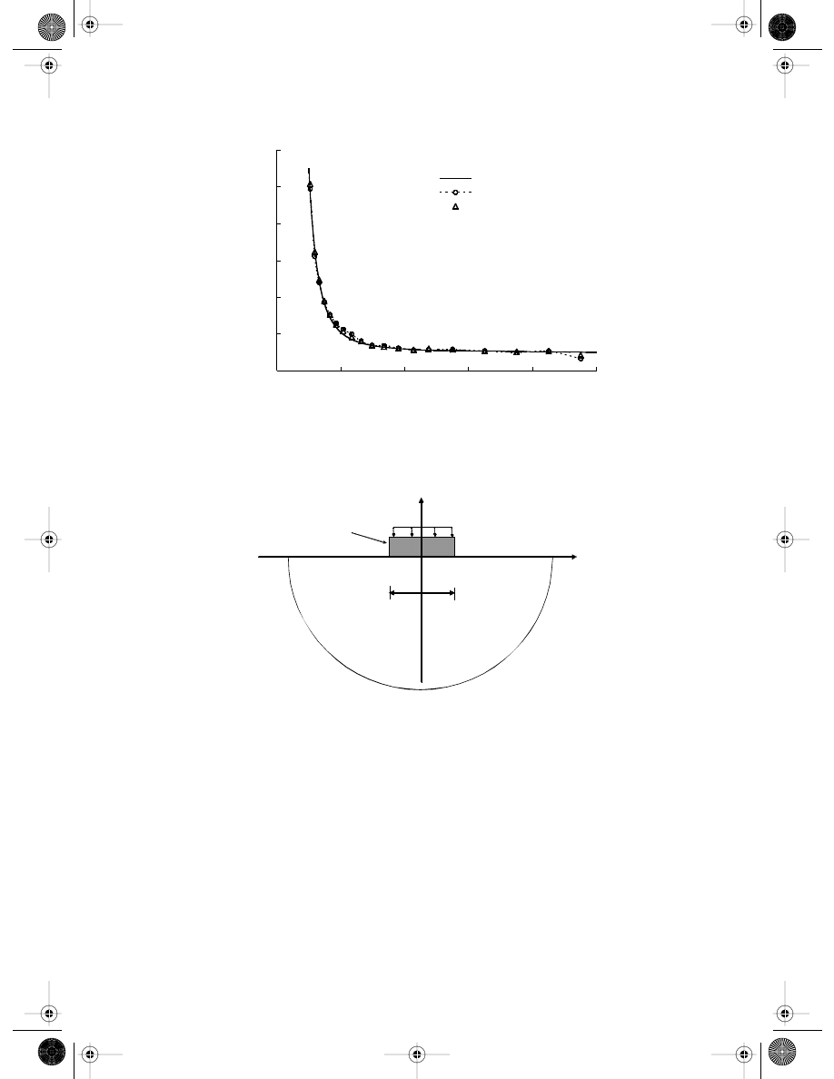
As the stress is more critical in assessment of the solution accuracy, detailed results of

stress are presented here. The stress

σ

x

at x = 0 obtained by BPIM is given in

Figure 13.5

together with the analytical solution for the infinite plate. It can be observed from this
figure that BPIM gives very good results for this problem. The BNM results of this problem
are also shown in the same figure for comparison. It is clearly shown that the BPIM and
BNM results possess nearly the same accuracy.

Example 13.3

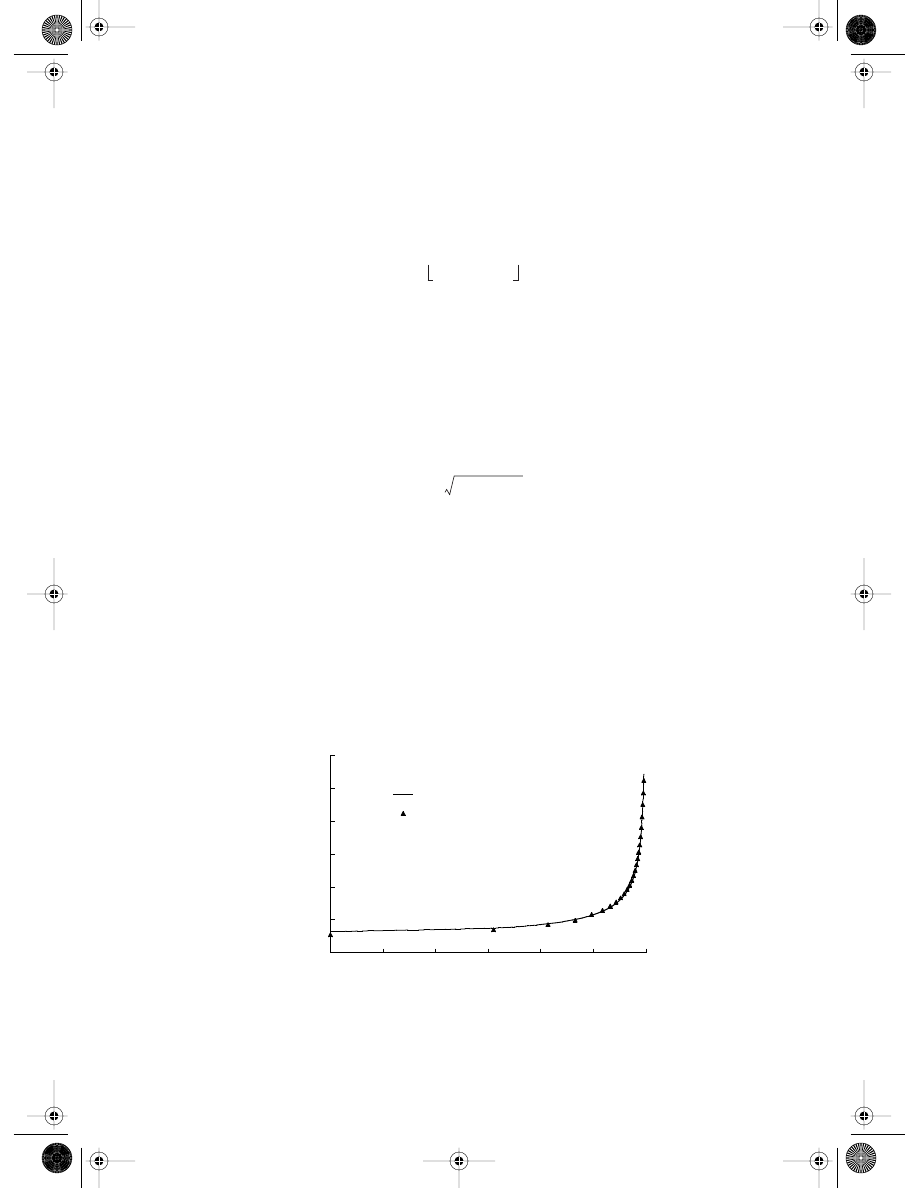
A Rigid Flat Punch on a Semi-Infinite Foundation

As BEM methods have a clear advantage over domain-type methods for problems with
infinite domain, BPIM is used to obtain a solution for an indentation produced by a rigid
flat punch in a semi-infinite soil foundation, as shown in

Figure 13.6.

In this case, Green’s

functions for a half-plane are employed (Brebbia et al., 1984), and only the contact surface
between the punch and half space needs to be discretized.

Consider a rigid punch of length L = 12 subjected to a uniform pressure of p = 100 on

the top surface. The parameters of the soil foundation are taken as E = 3.0

× 10

4

, and

ν = 0.3.

The punch is considered to be perfectly smooth, and does not result in any fraction force
in the interface between the punch and the foundation. An indentation is measured by
the vertical displacement of the punch. A plane strain condition is assumed. Due to
symmetry, only the right half of the contact surface is discretized by 31 distributed boundary

FIGURE 13.4
Nodes in a plate with a central hole subjected to a unidirectional tensile load in the x direction.

a=9

r=1

x

y

D

C

B

A

E

p

1238_Frame_C13.fm Page 554 Wednesday, June 12, 2002 5:27 PM

© 2003 by CRC Press LLC

nodes; 31 nonuniformly distributed integration background cells are used. Coordinates
of these boundary nodes are obtained using the following formula:

(13.30)

where m is the node number, and m = 1 to 31.

The vertical surface displacements of the foundation are assumed to be the same of that

of the punch (perfect contact). This assumption is often proved true for a rigid punch.
A prescribed vertical displacement of the punch is imposed on the contact surface as a
boundary constraint. The prescribed displacement of the punch can be obtained using the

FIGURE 13.5
Stress distribution in the plate with a central hole subjected to a unidirectional tensile load (

σ

x

, at x

= 0). (From

Gu, Y. T. and Liu, G. R., Comput. Mech., 28, 47–54, 2002. With permission.)

FIGURE 13.6
Rigid punch forced on a semi-infinite soil foundation. (From Gu, Y. T. and Liu, G. R., Comput. Mech., 28, 47–54,
2002. With permission.)

0.8

1.2

1.6

2.0

2.4

2.8

3.2

0

2

4

6

8

10

y

Stress

Analytical solution
BPIM
BNM

L

p

y

x

Soil

Rigid punch

x

m

6.2 m 1

–

(

)

m

--------------------------

=

1238_Frame_C13.fm Page 555 Wednesday, June 12, 2002 5:27 PM

© 2003 by CRC Press LLC

approximate method presented by Poulos and Davis (1974); i.e., the vertical displacement
of a vertically loaded rigid area in contact with the rigid punch may be approximated by
the mean vertical displacement of a uniformly loaded flexible area of the same shape. The
approximation is expressed as follows:

(13.31)

where v

rigid

is the vertical displacement of the rigid area in contact with the rigid punch,

v

center

and v

edge

are vertical displacements at the center and edge, respectively, of the contact

area subjected to uniform load, when the contact area is considered flexible. The analytical
solution of v

center

and v

edge

can be obtained in the textbook by Timoshenko and Goodier

(1977). The exact solution (Poulos and Davis, 1974) of contact stresses along the contact
surface is

(13.32)

BPIM is utilized to obtain the contact stresses along the contact surface. The support

domain of a quadrature point is determined by Equation 13.17 (with

α

s

= 2.0, and the

characteristic arc-length of d

Q

= 3.0). If the number of nodes in the support domain is

more than six, only six nodes with shorter arc-length to the quadrature point are used in
the interpolation. When these six nodes are all on one side of the quadrature point along
the boundary, one more node nearest to this evaluation point in the other side is purposely
added to the support domain to avoid an extrapolation.

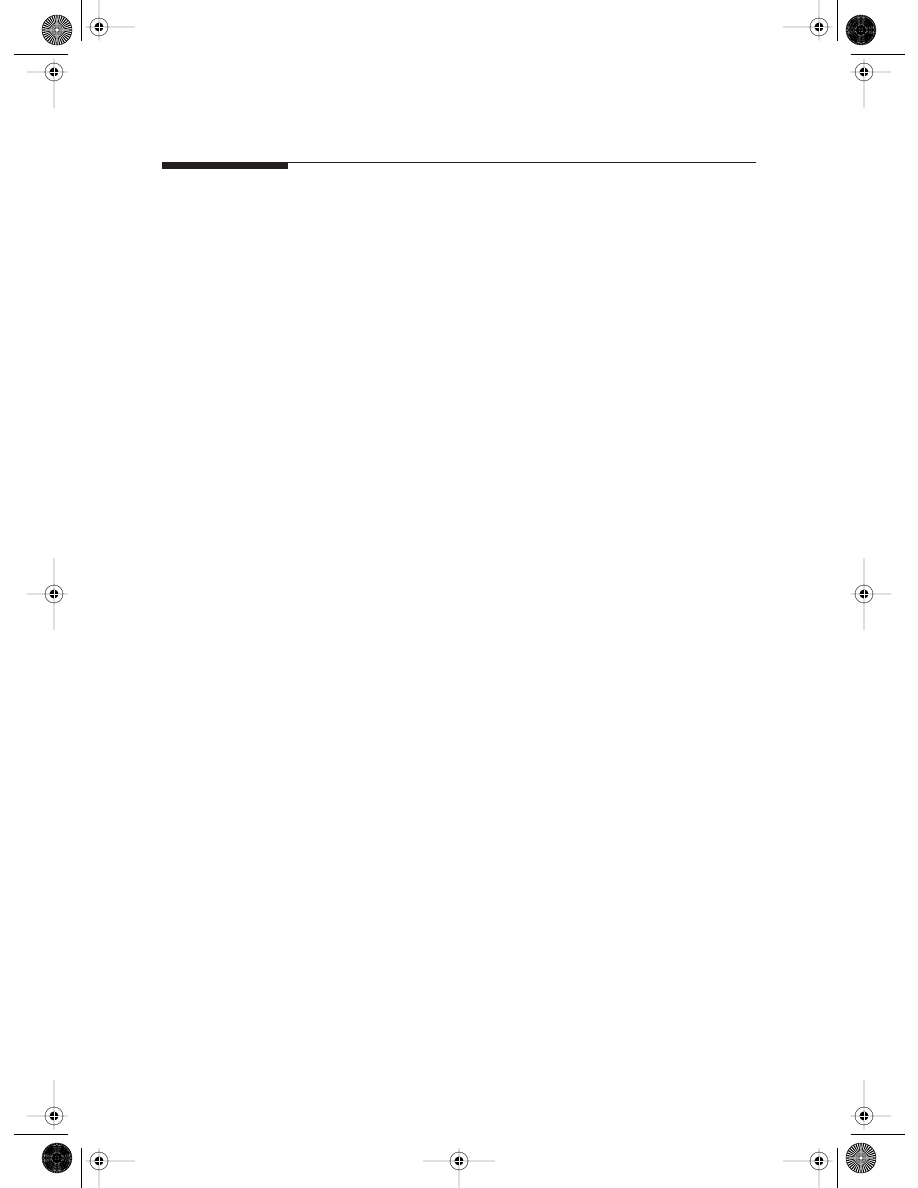
Figure 13.7 plots the comparison between the contact stresses calculated analytically

and by the BPIM along the contact surface. The plot shows excellent agreement between
the analytical and numerical results.

FIGURE 13.7
Contact stresses on the contact surface between the punch and the half-space. (From Gu, Y. T. and Liu, G. R.,
Comput. Mech., 28, 47–54, 2002. With permission.)

v

rigid

1
2

---

v

center

v

edge

+

flexible

=

σ

y

p

-----

2

π

---

1

1

2x

/L

(

)

2

–

--------------------------------

=

0

1

2

3

4

5

6

0

1

2

3

4

5

6

Analytical
BPIM

x

s

y

/p

1238_Frame_C13.fm Page 556 Wednesday, June 12, 2002 5:27 PM

© 2003 by CRC Press LLC

13.2 BPIM Using Radial Function Basis

For 2D problems, the boundaries of the domain are curves. Therefore, the PIM shape
function using polynomial basis will have no problem, and BPIM works perfectly well
without any special efforts. For 3D problems for which 2D shape functions need to be
constructed, there could be an issue of singular moment matrices. The special techniques
discussed in Section 5.6 should be applied. One effective way is to use RPIM shape
functions. This section introduces the boundary MFree method using RPIM shape func-
tions. This method was formulated and coded by Gu and Liu (2001a) and termed as
BRPIM. Although BRPIM performs no better than BPIM for 2D problems, its full advan-
tages are expected to be seen for 3D problems.

The formulation procedure for BRPIM is largely the same as that of BPIM, except for

the formulation of the shape function. This section, therefore, focuses only on the portion
of the formulation that is different from BPIM. As the radial function is used, a study on
the effects of these parameters of the radial function is performed. The performance of
BRPIM is discussed using example problems of 2D elastostatics.

13.2.1

Radial Basis Point Interpolation

In BRPIM, the radial basis functions R

i

(s) listed in

Table 5.1

are used. The point interpo-

lation for displacement u(s) and traction t(s) at a point s on the boundary

Γ from the

surrounding nodes uses radial basis functions, i.e.,

(13.33)

(13.34)

where s is a curvilinear distance (the arc-length for a 1D curve boundary) on

Γ, n is the

number of nodes in the support domain of a point of interest s

Q

, which is usually the

quadrature point, R

i

(s) is a radial basis function, and

α

i

and

β

i

are the coefficients. In matrix

form, we have

αααα

T

=

[

α

1

,

α

2

,

α

3

,…,

α

n

]

(13.35)

ββββ

T

=

[

β

1

,

β

2

,

β

3

,…,

β

n

]

(13.36)

The following multiquadrics (MQ) radial function is used in this section:

(13.37)

Two parameters, q and C, need to be determined in an MQ radial function. Detailed

investigations of these parameters are given in the following numerical examples.

The coefficients

α

i

and

β

I

can be determined by enforcing Equations 13.33 and 13.34 to

be satisfied at the n-node support domain of point s

Q

. Equations 13.33 and 13.34 can then

be written in the following matrix form:

u

n

= R

Q

ααα

α

(13.38)

t

n

= R

Q

ββββ

(13.39)

u

R

i

s

( )

α

i

i

=1

n

∑

R

T

s

( )ααα

α

=

=

t

R

i

s

( )

β

i

i

=1

n

∑

R

T

s

( )ββββ

=

=

R

i

s

( )

s

i

2

C

2

+

(

)

q

=

1238_Frame_C13.fm Page 557 Wednesday, June 12, 2002 5:27 PM

© 2003 by CRC Press LLC

where u

n

and t

n

are the vectors of nodal displacements and tractions in the support domain,

given by

u

n

=

[u

1

, u

2

, u

3

, ,u

n

]

T

(13.40)

t

n

=

[t

1

, t

2

, t

3

, ,t

n

]

T

(13.41)

and R

Q

is the moment matrix of radial basis functions

(13.42)

Solving

ααα

α and ββββ from Equations 13.38 and 13.39, and then substituting them back into

Equations 13.33 and 13.34, we obtain

u

(s) = Φ

Φ

Φ

Φ

T

(s)u

n

(13.43)

t

(s) = Φ

Φ

Φ

Φ

T

(s)t

n

(13.44)

where the shape function

Φ

Φ

Φ

Φ(s) is defined by

Φ

Φ

Φ

Φ

T

(s) = R

T

(s)R

Q

=

[

φ

1

(s),

φ

2

(s),

φ

3

(s), ,

φ

n

(s)]

(13.45)

Similar to the polynomial basis shape functions, the shape function

φ

i

(s) obtained through

the above procedure satisfies

φ

i

(s = s

i

) = 1 i = 1, n

(13.46)

φ

j

(s = s

i

)

= 0 j ≠ i

(13.47)

(13.48)

Therefore, the RPIM shape functions constructed have the Kronecker delta function prop-
erty, and the boundary conditions can be easily imposed as in traditional BEM.

The moment matrix R

Q

is an n

× n matrix. It must be invertible for the construction of

the shape functions in Equation 13.45. The existence of

has been proved for arbitrary

scattered nodes (Kansa, 1990a,b). Therefore, in BRPIM, interpolation using the radial basis
function is stable and flexible for arbitrarily distributed nodes on the boundary of the
problem domain. This advantage will be very beneficial when using BRPIM to solve 3D
problems.

13.2.2

BRPIM Formulation

The formulation of system equations in BRPIM is exactly the same as that for BPIM, except
that the PIM shape function given by Equation 13.13 is replaced by the RPIM shape
function defined by Equation 13.45.

…

…

R

Q

R

1

s

1

( ) R

2

s

1

( ) … R

n

s

1

( )

R

1

s

2

( ) R

2

s

2

( ) … R

n

s

2

( )

M

M

O

M

R

1

s

n

( ) R

2

s

n

( )

… R

n

s

n

( )

=

R

Q

1

–

…

φ

i

s

( )

i

=1

n

∑

1

=

R

Q

−1

1238_Frame_C13.fm Page 558 Wednesday, June 12, 2002 5:27 PM

© 2003 by CRC Press LLC

13.2.3

Comparison of BPIM, BNM, and BEM

A comparison of BPIM, BNM, and BEM is summarized concisely in Table 13.2. It can be
found that BPIM, BNM, and BEM are all based on the BIE. The difference is essentially
in the means of implementation.

BPIM vs. BEM
Both BPIM and BEM use polynomial interpolants, in which the number of monomials
used in the base functions, m, is the same as the number of nodes, n, utilized. Therefore,
the interpolant functions possess the delta function property. The boundary conditions
can be implemented with ease.

However, BPIM is a boundary-type MFree method, whereas BEM is a boundary-type

method based on boundary elements. As other MFree methods (e.g., EFG, BNM, MLPG),
the interpolation procedure in BPIM is based only on a group of arbitrary distributed
nodes. The interpolation at a quadrature point in BPIM is performed over the support
domain of the point, which may overlap with the support domains of other quadrature
points, as shown in Figure 13.8. BEM defines the shape functions over predefined regions
called elements, and there is no overlapping or gap between the elements.

TABLE 13.2

Comparison of BPIM, BRPIM, BNM, and BEM

BPIM

BRPIM

BNM

BEM

Mesh

No

No

No

Yes

Interpolants

Polynomial PIM

Radial PIM

MLS

Element based

polynomial

Interpolation area

based on

Distributed nodes Distributed nodes Distributed nodes

Element

Number of basis m and

interpolation nodes n

m = n

m = n

m

≠ n

m = n

Overlapping of

interpolation area

Overlapping

Overlapping

Overlapping

No overlapping

Shape function

Simple

Simple

Complicated

Simple

Delta property of shape

function

Yes

Yes

No

Yes

Application of boundary

conditions

Easy

Easy

Difficult

Easy

Number of system

equations

2N

B

2N

B

4N

B

2N

B

Source: Gu, Y. T. and Liu, G. R., Comput. Mech., 28, 47–54, 2002. With permission.

FIGURE 13.8
Interpolation in BPIM and BRPIM.

Ä

Ä

Ä

boundary

boundary nodes

quadrature points

support domains for quadrature points

1238_Frame_C13.fm Page 559 Wednesday, June 12, 2002 5:27 PM

© 2003 by CRC Press LLC

BPIM vs. BNM
Both BPIM and BNM are boundary-type MFree methods. The difference between these
two methods comes from the different interpolants utilized. As discussed above, BPIM
uses PIM shape functions, in which the coefficients a and b in Equation 13.1 are constant.
The MLS interpolants are used in BNM, in which a and b are also functions of curvilinear
coordinate s. Therefore, the shape function of BNM is more complicated than PIM. In
addition, the shape function of BNM constructed using MLS approximation lacks the delta
function property. It takes extra effort to impose boundary conditions.

13.2.4

Numerical Examples

Example 13.4

Cantilever Beam

Example 13.1 is used here again to examine BRPIM. All the parameters are exactly the
same.

Effects of Radial Function Parameters
Two parameters,

α

C

and q, in the MQ radial function defined in

Table 5.3

are investigated

to reveal their effects on the performance of BRPIM. The characteristic length d

c

is taken

to be the “average” nodal spacing for nodes in the support domain of the quadrature
point.

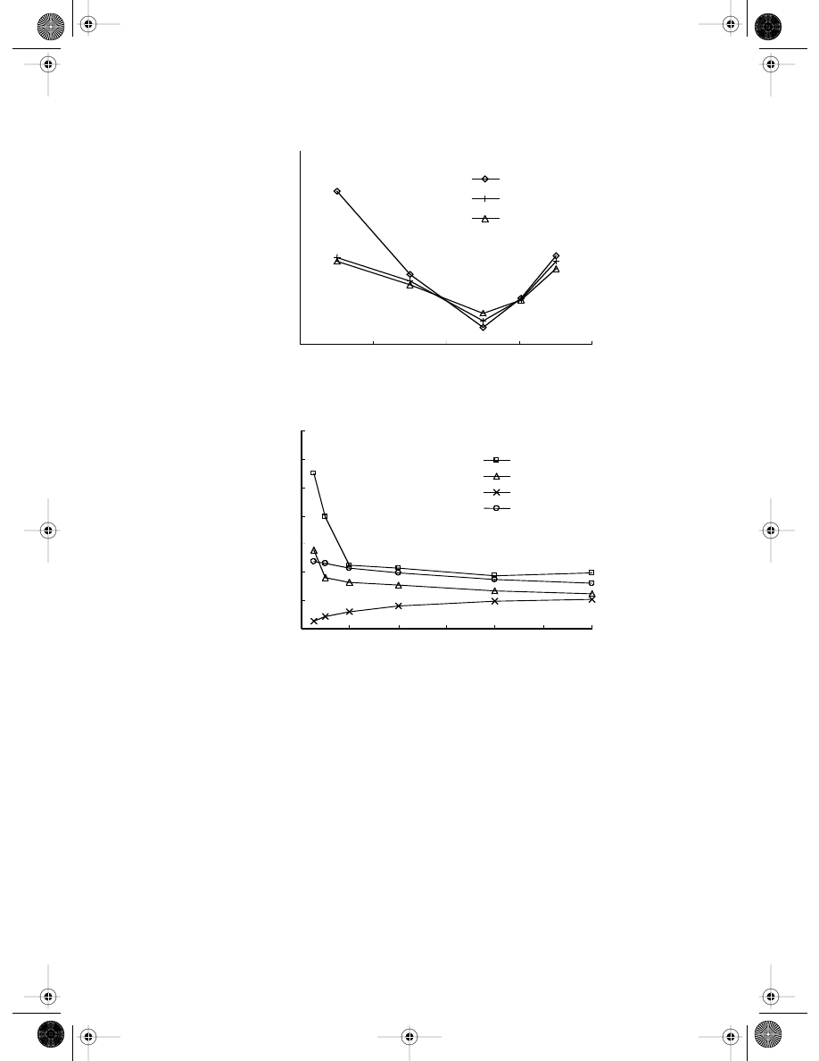
The parameter q is first investigated, and q is taken to be

−1.5, −0.5, 0.5, and 1.5. Shear

stresses for different q are obtained and compared with the analytical solution. Errors for
different q are plotted in

Figure 13.9a.

This figure shows that q = 0.5 leads to a better result

in the range of studies. Hence, 0.5 is used in following studies.

Errors in shear stresses of different

α

C

are plotted in Figure 13.9b. It is found that

α

C

can

be chosen from a wide range of

α

C

= 1.0 to 1.6, where steadily accurate results can be

obtained. For convenience,

α

C

= 1.2 is used in the following studies.

From studies for 2D interpolation, it has also been understood that

α

C

has a wider range

of choices, but parameter q is very critical and has to be very precise to obtain good results.
To determine a more precisely tuned q, more detailed study is required.

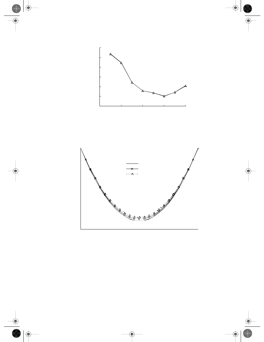
Effects of Interpolation Domain
The size of the support domain of a quadrature point is determined by the parameter

α

s

in Equation 13.17. Results of

α

s

= 1.0 to 5.0 are obtained and plotted in

Figure 13.10

.

It is

found that the results obtained using a support domain with

α

s

= 3.0 to 4.5, which covers

about 6 to 10 nodes, are very good. Too small a support domain (

α

s

< 2.5) will lead to

large error. This is because there are not enough nodes to perform interpolation for the
field variable. Too big a support domain (

α

s

> 4.5) will also lead to large error. This is

because there are too many nodes to perform interpolation, which results in a very complex
shape function and hence a complex integrand in computing the system equations.
Numerical integral error becomes very large. Therefore,

α

s

= 3.0 to 4.5 is recommended.

For convenience and consistency,

α

s

= 4.0 is used in the following studies.

Comparison with the case of using BPIM, for which

α

s

= 2.0 is the optimum (see

Table 13.1

)

reveals that BRPIM requires a larger support domain, and more points for interpolation.
This finding agrees with that for domain-type PIM and RPIM.

Figure 13.11

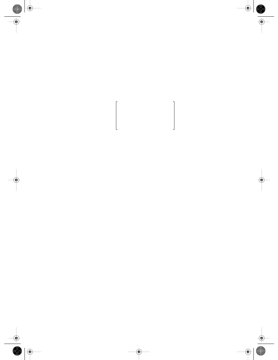
illustrates the comparison between the shear stress calculated analytically

and by the BRPIM at the section of x = L

/2. The plot shows good agreement between the

analytical and numerical results of BRPIM. The conventional linear BEM results of this

1238_Frame_C13.fm Page 560 Wednesday, June 12, 2002 5:27 PM

© 2003 by CRC Press LLC

problem are also shown in the same figure for comparison. The density of the nodes in
BEM and BRPIM is exactly the same. It is clearly shown that the BRPIM results are more
accurate than the BEM results. This is because the BRPIM uses more nodes for the inter-
polation of the displacements and tractions.

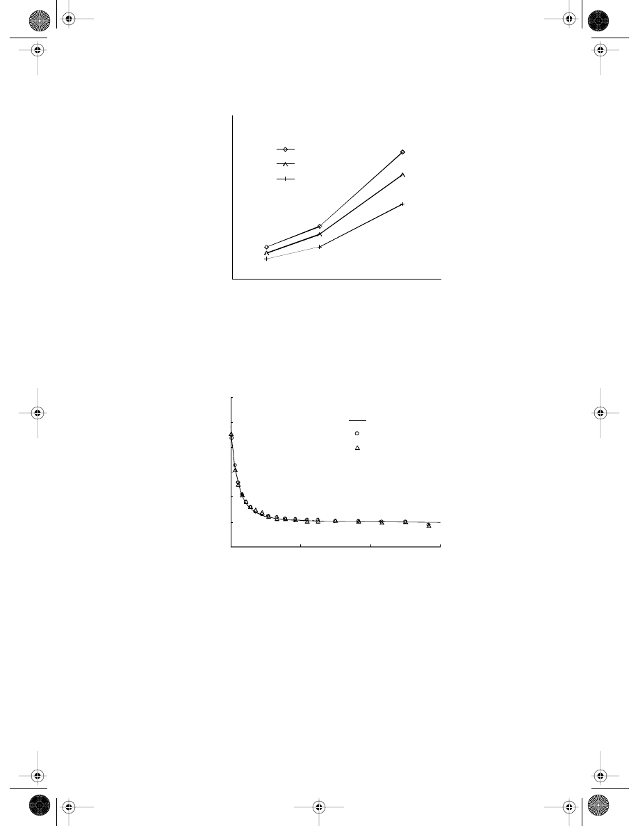
The convergence for the shear stresses at the section of x = L

/2 with node/mesh refine-

ment is shown in

Figure 13.12,

where h is a characteristic length relating the spacing of

the nodes. Three kinds of nodal arrangement of 72, 240, and 480 uniform boundary nodes
are used. The convergences of BNM and conventional linear BEM are also shown in the
same figure. It is observed that the convergence of BRPIM is very good. It can also be
observed that BRPIM has higher accuracy than BEM and BNM for this example.

FIGURE 13.9
Effect of parameters q and

α

C

of MQ radial basis function on the error of shear stress in the cantilever beam

computed using BRPIM. e

t

is defined by Equation 13.29. (a) Effect of q; (b) effect of

α

C

.

0.0E+00

5.0E-03

1.0E-02

1.5E-02

2.0E-02

2.5E-02

-2

-1

0

1

2

a

C

= 0.84

a

C

= 1.0

a

C

= 1.19

e

t

q

(a)

(b)

0.0E+00

5.0E-03

1.0E-02

1.5E-02

2.0E-02

2.5E-02

3.0E-02

3.5E-02

0

1

1.2

1.3

1.4

1.5

1.6

q

= -1.5

q

= -0.5

q

= 0.5

q

= 1.5

a

C

e

t

1238_Frame_C13.fm Page 561 Wednesday, June 12, 2002 5:27 PM

© 2003 by CRC Press LLC

Example 13.5

Plate with a Hole

Example 13.2 is also used to examine BRPIM. All the parameters are exactly the same. The
nodal distribution is shown in

Figure 13.4.

The stress

σ

x

at x = 0 computed using the BRPIM

code is given in

Figure 13.13

together with the analytical solution for the infinite plate.

The BEM results of this problem are also shown in the same figure for comparison. It can
be observed from this figure that the BRPIM gives very good results. It is clearly shown
that the BRPIM and BEM results possess nearly the same accuracy for this problem.

FIGURE 13.10
Influence of the parameter

α

s

of the interpolation domain.

FIGURE 13.11
Shear stress at the section x = L

/2 of the cantilever beam. Comparison of results obtained by three methods.

3.5E-03

4.0E-03

4.5E-03

5.0E-03

5.5E-03

6.0E-03

6.5E-03

1

2

3

4

5

α

s

e

t

-140

-120

-100

-80

-60

-40

-20

0

-6

-4

-2

0

2

4

6

Analytical
BRPIM
BEM

y

τ

xy

1238_Frame_C13.fm Page 562 Wednesday, June 12, 2002 5:27 PM

© 2003 by CRC Press LLC

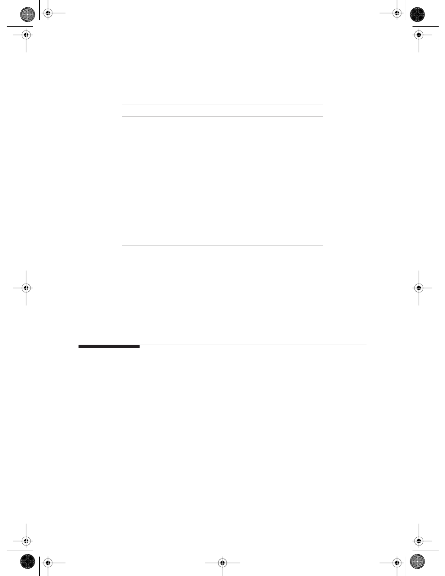
Example 13.6

Internally Pressurized Hollow Cylinder

A hollow cylinder under internal pressure shown in

Figure 13.14

is considered. The param-

eters are taken as p = 100, G = 8000, and

ν = 0.25. This problem has been used by several

other authors (see, e.g., Brebbia, 1978) as a benchmark problem, as the analytical solution
is available. Due to the symmetry of the problem, only one quarter of the cylinder needs
to be modeled. The arrangement of the field nodes is shown in

Figure 13.15.

The boundary

FIGURE 13.12
Convergence in e

t

norm of error.

FIGURE 13.13
Stress

σ

x

distribution in a plate with a central hole subjected to a unidirectional tensile load. Comparison of

results obtained using three different methods.

-3.0

-2.5

-2.0

-1.5

-1.0

-0.5

0.0

-0.8

-0.6

-0.4

-0.2

0

0.2

0.4

BEM

BNM

BRPIM

Log(h)

Log(

e

t

)

0.5

1.0

1.5

2.0

2.5

3.0

3.5

1

4

7

10

Analytical

BRPIM

BEM

y

a

x

1238_Frame_C13.fm Page 563 Wednesday, June 12, 2002 5:27 PM

© 2003 by CRC Press LLC

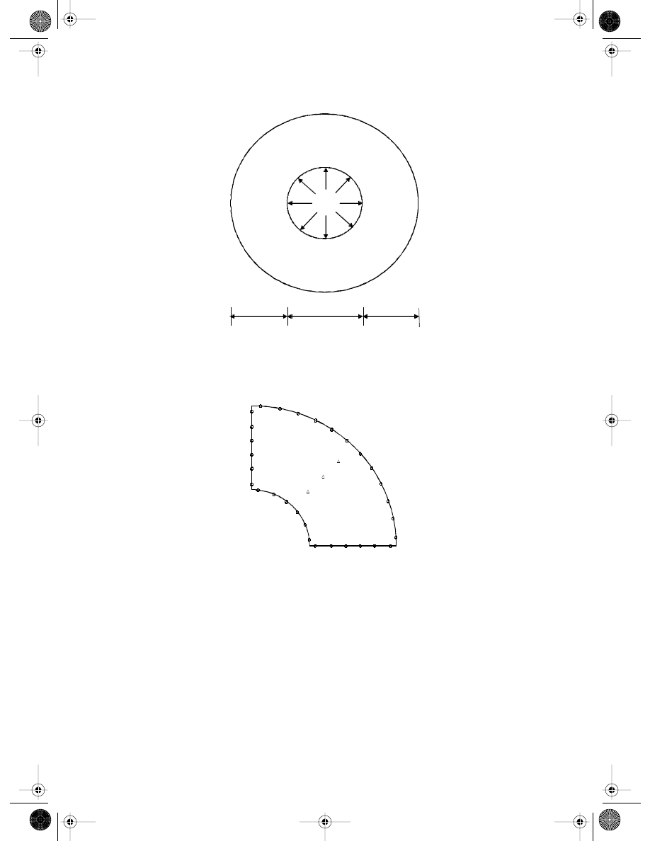
of this domain is discretized by 30 nodes (6 uniformly distributed nodes on ab, cd, and ad
and 12 uniformly distributed nodes on bc). The same number of background cells are used
for integration. Three internal points A, B, and C are selected for examination. The polar
coordinates (with the origin at the center of the cylinder) for the three internal points are
A(13.75,

π/4), B(17.5, π/4), and C(21.25, π/4). The dimensionless size of the support domain

of

α

s

= 2.0 is used for all the quadrature points in the integration on the boundary.

The BRPIM and BPIM results are compared with those obtained using BNM, conven-

tional BEM, and the analytical solution. The radial displacements at some of the boundary
nodes and the three internal points are listed in

Table 13.3.

The circumferential stresses

FIGURE 13.14
Hollow cylinder subjected to internal pressure.

FIGURE 13.15
Arrangement of nodes for a quarter model of the hollow cylinder.

p

15 20 15

1

2

3

24

23

22

A

B

C

a

b

c

d

1238_Frame_C13.fm Page 564 Wednesday, June 12, 2002 5:27 PM

© 2003 by CRC Press LLC

σ

θ

at points A, B, and C are also listed in the same table. The BRPIM and BPIM results are

in very good agreement with the analytical solution. In comparison with the conventional
BEM results, the BRPIM and BPIM solution is, in general, more accurate for both displace-
ments and stresses.

13.3 Remarks

Boundary MFree methods are presented in this chapter. Detailed formulations for BPIM
and BRPIM are provided for solving 2D problems of elastostatics. The boundary integral
equation is discretized using radial MFree shape functions based on a group of arbitrarily
distributed points on the boundary of the problem domain. The boundary MFree methods
do not require any element connectivity in constructing shape functions, and possess the
dimensionality advantage. Numerical examples have demonstrated that boundary MFree
methods are superior to conventional BEM in terms of accuracy.

Compared with the BNM, BPIM and BRPIM have the following advantages:

• BPIM is computationally much less expensive than BNM because of its simpler

interpolation scheme and smaller system equation dimension. The number of
system equations in BPIM is only a half of that in BNM.

• The imposition of boundary conditions is easy in BPIM and BRPIM because the

shape functions have the delta property.

• Rigid body movement can be used to avoid some singular integrals.

TABLE 13.3

Radial Displacement and Circumferential Stresses in the Pressurized
Hollow Cylinder

Nodes

Exact

BPIM BRPIM BNM

BEM

Radial Displacements (

× 10

−2

)

1

0.4464

0.4465

0.4466

0.4462

0.4468

2

0.4464

0.4478

0.4475

0.4463

0.4482

3

0.4464

0.4491

0.4493

0.4498

0.4494

22

0.8036

0.8213

0.8200

0.8220

0.8266

23

0.8036

0.8214

0.8207

0.8215

0.8268

24

0.8036

0.8199

0.8215

0.8223

0.8251

A

0.6230

0.6274

0.6211

0.6256

0.6319

B

0.5294

0.5342

0.5366

0.5353

0.5374

C

0.4766

0.4809

0.4810

0.4826

0.4838

Stress

σ

θ

A

82.0113

81.8947

82.1437

81.8513

82.0192

B

57.9226

58.1285

58.2585

58.1627

58.1691

C

45.4112

45.6471

45.6264

45.4597

45.6575

Source: Gu, Y. T. and Liu, G. R., Comput. Mech., 28, 47–54, 2002. With permission.

1238_Frame_C13.fm Page 565 Wednesday, June 12, 2002 5:27 PM

© 2003 by CRC Press LLC

The parameters for BPIM and BRPIM should be as follows:

• In using BPIM,

α

s

= 2.0 to 3.0 (with n = 3 to 6) yields acceptable results.

• In using BRPIM with MQ radial function, q = 0.5 and

α

C

= 1.0 to 1.6 lead to

acceptable results for most problems studied. q = 0.5 and

α

C

= 1.2 are recom-

mended. The dimensionless size of the support domain of

α

s

= 3.0 to 4.5 should

work for most problems.

BPIM and BRPIM need to be extended for 3D problems to take full advantages of the

meshless concept. For 2D problems, BPIM is the simplest method; it performs the best
and is very stable, without any kind of problem.

1238_Frame_C13.fm Page 566 Wednesday, June 12, 2002 5:27 PM

© 2003 by CRC Press LLC