Hahnel ABCs of Political Economy Modern Primer

Contents

List of Illustrations

Preface

Acknowledgements

1 Economics and Liberating Theory

People and Society

The Human Center

The Laws of Evolution Reconsidered

Natural, Species, and Derived Needs and Potentials

Human Consciousness

Human Sociability

Human Character Structures

The Relation of Consciousness to Activity

The Possibility of Detrimental Character Structures

The Institutional Boundary

Why Must There Be Social Institutions?

Complementary Holism

Four Spheres of Social Life

Relations Between Center, Boundary and Spheres

Social Stability and Social Change

Agents of History

2 What Should We Demand from Our Economy?

Economic Justice

Increasing Inequality of Wealth and Income

Different Conceptions of Economic Justice

Conservative Maxim 1

Liberal Maxim 2

Radical Maxim 3

Efficiency

The Pareto Principle

The Efficiency Criterion

Seven Deadly Sins of Inefficiency

Endogenous Preferences

Self-Management

Solidarity

Variety

Environmental Sustainability

Conclusion

A Simple Corn Model

A Simple Corn Economy

Situation 1: Inegalitarian Distribution of Scarce Seed Corn 49

Autarky

Labor Market

Credit Market

Situation 2: Egalitarian Distribution of Scarce Seed Corn

Autarky

Labor Market

Credit Market

Conclusions from the Simple Corn Model

Generalizing Conclusions

Economic Justice in the Simple Corn Model

Markets: Guided by an Invisible Hand or Foot?

How Do Markets Work?

What is a Market?

The “Law” of Supply

The “Law” of Demand72
The “Law” of Uniform Price

The Micro “Law” of Supply and Demand

Elasticity of Supply and Demand

The Dream of a Beneficent Invisible Hand80
The Nightmare of a Malevolent Invisible Foot

Externalities: The Auto Industry

Public Goods: Pollution Reduction

The Prevalence of External Effects

Snowballing Inefficiency

Market Disequilibria

Conclusion: Market Failure is Significant

Markets Undermine the Ties that Bind Us

Micro Economic Models

103

The Public Good Game

103

The Price of Power Game

106

The Price of Patriarchy

109

Conflict Theory of the Firm

111

The ABCs of Political Economy

Income Distribution, Prices and Technical Change

112

The Sraffa Model

114

Technical Change in the Sraffa Model

118

Technical Change and the Rate of Profit

123

A Note of Caution

125

Macro Economics: Aggregate Demand as Leading Lady 128
The Macro “Law” of Supply and Demand

128

Aggregate Demand132

Consumption Demand133
Investment Demand133
Government Spending

135

The Pie Principle

136

The Simple Keynesian Closed Economy Macro Model

137

Fiscal Policy

140

The Fallacy of Say’s Law

141

Income Expenditure Multipliers

143

Other Causes of Unemployment and Inflation

147

Myths About Inflation

150

Myths About Deficits and the National Debt

152

The Balanced Budget Ploy

154

Wage-Led Growth

157

Money, Banks, and Finance

160

Money: A Problematic Convenience

160

Banks: Bigamy Not a Proper Marriage

162

Monetary Policy: Another Way to Skin the Cat

168

The Relationship Between the Financial and “Real”
Economies

171

International Economics: Mutual Benefit
or Imperialism?

175

Why Trade Can Increase Global Efficiency

176

Comparative, Not Absolute Advantage Drives Trade

177

Why Trade Can Decrease Global Efficiency

180

Inaccurate Prices Misidentify Comparative
Advantages

181

Unstable International Markets Create Macro
Inefficiencies

182

Adjustment Costs Are Not Always Insignificant

183

Dynamic Inefficiency

183

Contents

vii

Why Trade Usually Aggravates Global Inequality

184

Unfair Distribution of the Benefits of Trade Between
Countries

185

Unfair Distribution of the Costs and Benefits of
Trade Within Countries

187

Why International Investment Can Increase Global
Efficiency

190

Why International Investment Can Decrease Global
Efficiency

191

Why International Investment Usually Aggravates
Global Inequality

193

The Balance of Payments Accounts

198

Open Economy Macro Economics and IMF
Conditionality Agreements

201

Macro Economic Models

208

Bank Runs

208

International Financial Crises

211

International Investment in a Simple Corn Model

212

Banks in a Simple Corn Model

216

Imperfect Lending Without Banks

216

Lending With Banks When All Goes Well

217

Lending With Banks When All Does Not Go Well

218

International Finance in an International Corn Model

219

Fiscal and Monetary Policy in a Closed Economy Macro
Model

220

IMF Conditionality Agreements in an Open Economy
Macro Model

225

Wage-Led Growth in a Long Run, Political Economy
Macro Model

231

The General Framework

231

A Keynesian Theory of Investment

235

A Marxian Theory of Wage Determination

235

Solving the Model

236

An Increase in Capitalists’ Propensity to Save

238

An Increase in Capitalists’ Propensity to Invest

240

An Increase in Workers’ Bargaining Power

240

What Is To Be Undone? The Economics of
Competition and Greed

242

Free Enterprise Equals Economic Freedom – Not

242

viii

The ABCs of Political Economy

Free Enterprise is Efficient – Not

248

Biased Price Signals

249

Conflict Theory of the Firm

249

Free Enterprise Reduces Economic Discrimination – Not

251

Free Enterprise is Fair – Not

253

Markets Equal Economic Freedom – Not

254

Markets Are Fair – Not

257

Markets Are Efficient – Not

258

What Went Wrong?

261

What Is To Be Done? The Economics of Equitable
Cooperation

265

Not All Capitalisms Are Created Equal

265

Taming Finance

266

Full Employment Macro Policies

267

Industrial Policy

268

Wage-Led Growth

270

Progressive Not Regressive Taxes

270

Tax Bads Not Goods

272

A Mixed Economy

272

Living Wages

274

A Safe Safety Net

276

Worker and Consumer Empowerment

277

Beyond Capitalism

278

Replace Private Ownership with Workers’
Self-Management

279

Replace Markets with Democratic Planning

280

Participatory Economics

282

Reasonable Doubts

284

Conclusion

291

Index

293

Contents

Economics and Liberating
Theory

Unlike mainstream economists, political economists have always
tried to situate the study of economics within the broader project of
understanding how society functions. However, during the second
half of the twentieth century dissatisfaction with the traditional
political economy theory of social change known as historical
materialism increased to the point where many modern political
economists and social activists no longer espouse it, and most who
still call themselves historical materialists have modified their theory
considerably to accommodate insights about the importance of
gender relations, race relations, and the “human factor” in under-
standing social stability and social change. The liberating theory
presented briefly in this chapter attempts to transcend historical
materialism without throwing out the baby with the bath water. It
incorporates insights from feminism, national liberation and anti-
racist movements, and anarchism, as well as from mainstream
psychology, sociology, and evolutionary biology where useful.
Liberating theory attempts to understand the relationships between
economic, political, kinship and cultural activities, and the forces
behind social stability and social change, in a way that neither over
nor underestimates the importance of economic dynamics, and
neither over nor underestimates the importance of human agency
compared to social forces.

PEOPLE AND SOCIETY

People usually define and fulfill their needs and desires in coopera-
tion with others – which makes us a social species. Because each of us
assesses our options and chooses from among them based on our

1. For a fuller treatment see Liberating Theory (South End Press, 1986) by

Michael Albert, Leslie Cagan, Noam Chomsky, Robin Hahnel, Mel King,
Lydia Sargent, and Holly Sklar.

evaluation of their consequences we are also a self-conscious species.
Finally, in seeking to meet the needs we identify today, we choose to
act in ways that sometimes change our human characteristics, and
thereby change our needs and preferences tomorrow. In this sense
people are self-creative.

Throughout history people have created social institutions to help

meet their most urgent needs and desires. To satisfy our economic
needs we have tried a variety of arrangements – feudalism,
capitalism, and centrally planned “socialism” to name a few – that
assign duties and rewards among economic participants in different
ways. But we have also created different kinds of kinship relations
through which people seek to satisfy sexual needs and accomplish
child rearing goals, as well as different religious, community, and
political organizations and institutions for meeting cultural needs
and achieving political goals. Of course the particular social arrange-
ments in different spheres of social life, and the relations among them,
vary from society to society. But what is common to all human
societies is the elaboration of social relationships for the joint iden-
tification and pursuit of individual need fulfillment.

To develop a theory that expresses this view of humans – as a self-

conscious, self-creative, social species – andthis view of society – as
a web of interconnectedspheres of social life – we first concentrate
on concepts helpful for thinking about people, or the human center;
next on concepts that help us understand social institutions, or the
institutional boundary within which individuals function; and finally
on the relationship between the human center andinstitutional
boundary, and the possible relations between four spheres of social life.

THE HUMAN CENTER

Except for creationists most consider the laws of evolution straight-
forward and non-controversial. Unfortunately popular inter-
pretations that emphasize the advantages of aggression and strength,
but neglect equally important factors for passing on one’s genes like
good parenting skills and successful cooperation, sprinkle more
ideology over the scientific basis of Darwin’s theory of evolutionary
biology than most realize.

The laws of evolution reconsidered

Human nature as it now exists was formed in accord with the laws
of evolution under conditions pertaining well before recorded

The ABCs of Political Economy

human history. Fossils discovered in Ethiopia and Kenya now date
human ancestors back at least 5 or 6 million years. Distinctly human
species arose in Africa at least 2 million years ago, while present
evidence indicates that modern humans are only about 100,000
years old. Therefore the conditions relevant to which genetic
mutations were advantageous and which were not are the conditions
prevailing in central Africa between 6 million and 100,000 years ago.
It is often noted that the last 10,000 years of human history – so
called “historic time,” the time period we know much about – has
been fraught with war, conquest, genocide, and slavery. And it is
often speculated that under those conditions people with a genetic dis-
position to aggression and vengeance, for example, might have been
well suited to survival. But historic time is only a tenth of the time
modern humans have roamed the earth, and is only an evolution-
ary instant compared to the 6 million years during which the human
species evolved from our common ancestry with apes and chim-
panzees. This means it is impossible for the historical conditions we
know something about to have selected genetic characteristics sig-
nificantly different from those humans already had 100,000 years
ago. Therefore, it is not possible that the human history we know
something about – our history of war, oppression, and exploitation
– has made our genetic “nature” hopelessly aggressive, vindictive, or
power hungry. Throughout the 10,000 years of recorded history we
have been, and remain, genetically what we were at the outset. To
believe otherwise is to believe that a baby plucked from the arms of
its mother, moments after birth, 10,000 years ago, and time-traveled
to the present would be genetically different from babies born today.
And this is simply not the case.

But what is the relevance of this to perceptions about “human

nature?” The point is that whether conditions during the past 10,000
years favored survival of the more aggressive and vindictive, or
survival of those who cooperated more successfully, is irrelevant to
what “human nature” is really like. Because the conditions during
known history played no role in forging our genetic nature. The
relevant conditions for speculations concerning genetic traits
promoting survival were the conditions that prevailed in Africa 6
million to 100,000 years ago. And whether or not the conditions
human ancestors lived in during that lengthy period favored genetic
traits conducive to aggression any more than traits conducive to
successful cooperation, is very much an open question.

Economics and Liberating Theory

This does not mean that our 10,000-year history of war,

oppression, andexploitation has hadno impact on people’s attitudes
andbehavior today. These aspects of our history have hadimportant
effects on our consciousness, culture, andsocial institutions that
cannot be ignoredor “willedaway.” But the point is that known
history has left ideological and institutional residues, not genetic
residues. Only conditions in Africa 6 million years ago had any
influence on genetic selection. So it is perfectly possible that under
institutional conditions that are very different from those we have
today, and the different expectations that go with them, that human
behavior – the combinedproduct of our genetic inheritance andour
institutional environment – couldbe quite d

ifferent than it is

presently. This simple fact is something apologists for capitalism
ignore when they argue that people are doomed to the economics of
competition and greed by “human nature.” Insteadit is just as plausible
that an economics of equitable cooperation is compatible with our
genetic make-up, and perfectly possible under different institutional
conditions – popular opinion to the contrary, not withstanding.

Natural, species, and derived needs and potentials

All people, simply by virtue of being human, have certain needs,
capacities, and powers. Some of these, like the needs for food and
sex, or the capacities to eat and copulate, we share with other living
creatures. These are our natural needs and potentials. Others, however,
such as the needs for knowledge, creative activity, and love, and the
powers to conceptualize, plan ahead, evaluate alternatives, and
experience complex emotions, are more distinctly human. These are
our species needs and potentials. Finally, most of our needs and powers,
like the desire for a particular singer’s recordings, or the need to share
feelings with a particular loved one, or the ability to play a guitar or
repair a roof, we develop over the course of our lives. These are our
derived needs and potentials.

In short, every person has natural attributes similar to those of

other animals, and species characteristics shared only with other
humans – both of which can be thought of as genetically “wired-
in.” Based on these genetic potentials people develop more specific
derived needs and capacities as a result of their particular life
experiences. While our natural and species needs and powers are the
results of past human evolution and are not subject to modification
by individual or social activity, our derived needs and powers are
subject to modification by individual activity and are very

The ABCs of Political Economy

dependent on our social environment – as explained below. Since a
few species needs and powers are especially critical to understanding
how humans and human societies work, I discuss them before
explaining how derived needs and powers develop.

Human consciousness

Human beings have intellectual tools that permit them to
understand and situate themselves in their surroundings. This is not
to say that everyone accurately understands the world and her
position in it. No doubt, most of us deceive ourselves greatly much
of the time! But an incessant striving to develop some interpretation
of our relationship with our surroundings is a characteristic of
normally functioning human beings. We commonly call the need
and ability to do this consciousness, a trait that makes human systems
much more complicated than non-human systems. It is conscious-
ness that allows humans to be self-creative – to select our activities
in light of their preconceived effects on our surroundings and
ourselves. One effect our activities have is to fulfill our present needs
and desires, more or less fully. But another effect of our activities is
to reinforce or transform our derived characteristics, and thereby the
needs and capacities that depend on them. Our ability to analyze,
evaluate, and take the human development effects of our choices
into account is why humans are the “subjects” as well as the
“objects” of our histories.

The human capacity to act purposefully implies the needto

exercise that capacity. Not only can we analyze andevaluate the
effects of our actions, we needto exercise choice over alternatives,
andwe therefore needto be in positions to do so. While some call
this the “needfor freedom,” it bears pointing out that the human
“needfor freedom” goes beyondthat of many animal species. There
are animals that cannot be domesticated or will not reproduce in
captivity, thereby exhibiting an innate “needfor freedom.” But the
human needto employ our powers of consciousness requires
freedom beyond the “physical freedom” some animal species require
as well. People require freedom to choose and direct their own
activities in accord with their understanding and evaluation of the
effects of that activity. In chapter 2 I will define the concept “self-
management” to express this peculiarly human species needin a
way that subsumes the better known concept “individual freedom”
as a special case.

Economics and Liberating Theory

Human sociability

Human beings are a social species in a number of important ways.
First, the vast majority of our needs and potentials can only be satisfied
and developed in conjunction with others. Needs for sexual and
emotional gratification can only be pursuedin relations with others.
Intellectual andcommunicative potentials can only be developedin
relations with others. Needs for camaraderie, community, and social
esteem can only be satisfiedin relation with others.

Second, needs and potentials that might, conceivably, be pursued

independently, seldom are. For example, people could try to satisfy
their economic needs self-sufficiently, but we seldom have done so
since establishing social relationships that define and mediate
divisions of duties and rewards has always proved so much more
efficient. And the same holds true for spiritual, cultural, and most
other needs. Even when desires might be pursued individually,
people have generally found it more fruitful to pursue them jointly.

Third, human consciousness contributes a special character to our

sociability. There are other animal species which are social in the
sense that many of their needs can only be satisfied with others. But
humans have the ability to understand and plan their activity, and
since we recognize this ability in others we logically hold them
accountable for their choices, and expect them to do likewise. Peter
Marin expressed this aspect of the human condition eloquently in an
essay titled “The Human Harvest” published in Mother Jones
(December, 1976: 38).

Kant called the realm of connection the kingdom of ends. Erich
Gutkind’s name for it was the absolute collective. My own term for
the same thing is the human harvest – by which I mean the webs
of connection in which all human goods are clearly the results of a
collective labor that morally binds us irrevocably to distant others.
Even the words we use, the gestures we make, and the ideas we
have, come to us already worn smooth by the labor of others, and
they confer upon us an immense debt we do not fully acknowledge.

Bertell Ollman explains it is the individualistic, not the social inter-
pretation of human beings that is absurdandunscientific when
examinedclosely (Alienation, Cambridge University Press, 1973: 108):

The individual cannot escape his dependence on society even
when he acts on his own. A scientist who spends his lifetime in a

The ABCs of Political Economy

laboratory may delude himself that he is a modern version of
Robinson Crusoe, but the material of his activity and the
apparatus and skills with which he operates are social products.
They are inerasable signs of the cooperation which binds men
together. The very language in which a scientist thinks has been
learned in a particular society. Social context also determines the
career and other life goals that an individual adopts. No one
becomes a scientist or even wants to become one in a society
which does not have any. In short, man’s consciousness of himself
and of his relations with others and with nature are that of a social
being, since the manner in which he conceives of anything is a
function of his society.

In sum, there never was a Hobbesian “state of nature” where indi-
viduals roamed the wilds in a “natural” state of war with one
another. Human beings have always lived in social units such as
tribes and clans. The roots of our sociality – our “realm of
connection” or “human harvest” – are both physical–emotional and
mental–conceptual. The unique aspect of human sociality is that the
“webs of connection” that inevitably connect all human beings are
woven not just by a “resonance of the flesh” but by a shared con-
sciousness and mutual accountability as well. Individual humans do
not exist in isolation from their species community. It is not possible
to fulfill our needs and employ our powers independently of others.
And we have never lived except in active interrelation with one
another. But the fact that human beings are inherently social does
not mean that all institutions meet our social needs and develop our
social capacities equally well. For example, in later chapters I will
criticize markets for failing to adequately account for, express and
facilitate human sociality.

Human character structures

People are more than their constantly developing needs and powers.
At any moment we have particular personality traits, skills, ideas,
and attitudes. These human characteristics play a crucial mediating
role. On the one hand they largely determine the activities we will
select by defining the goals of these activities – our present needs,
desires, or preferences. On the other hand, the characteristics
themselves are merely the cumulative imprint of our past activities
on our innate potentials. What is important regarding human char-
acteristics is to neither underestimate nor overestimate their

Economics and Liberating Theory

permanence. Although I have emphasized that people derive needs,
powers, and characteristics over their lifetimes as the result of their
activities, we are never completely free to do so at any point in time.
Not only are people limited by the particular menu of role offerings
of the social institutions that surround them, they are constrained at
any moment by the personalities, skills, knowledge, and values they
have accumulated as of that moment themselves. But even though
character structures may persist over long periods of time, they are
not totally invariant. Any change in the nature of our activities that
persists long enough can lead to changes in our personalities, skills,
ideas, and values, as well as changes in our derived needs and desires
that depend on them.

A full theory of human development would have to explain how

personalities, skills, ideas, and values form, why they usually persist,
but occasionally change, andwhat relationship exists between these
semi-permanent structures andpeople’s needs andcapacities. No such
psychological theory now exists, nor is visible on the horizon. But for-
tunately, a few “low level” insights are sufficient for our purposes.

The relation of consciousness to activity

The fact that our knowledge and values influence our choice of
activities is easy to understand. The manner in which our activities
influence our consciousness and the importance of this relation is
less apparent. A need that frequently arises from the fact that we see
ourselves as choosing among alternatives, is the need to interpret
our choices in a positive light. If we saw our behavior as completely
beyond our own control, there would be no need to justify it, even
to ourselves. But to the extent that we see ourselves as choosing
among options, it can be very uncomfortable if we are not able to
“rationalize” our decisions. This is not to say that people always
succeed in justifying their actions, even to themselves. Nor do all
circumstances make it equally easy to do so! Rather, the point is that
striving to minimize what some psychologists call “cognitive
dissonance” is a corollary of our power of consciousness. The
tendency to minimize cognitive dissonance creates a subtle duality
to the relationship between thought and action in which each
influences the other, rather than a unidirectional causality. When
we fulfill needs through particular activities we are induced to mold
our thoughts to justify or rationalize both the logic and merit of
those activities, thereby generating consciousness-personality

The ABCs of Political Economy

structures that can have a permanence beyond that of the activities
that formed them.

The possibility of detrimental character structures

An individual’s ability to mold her needs and powers at any moment
is constrained by her previously developed personality, skills, and
consciousness. But these characteristics were not always “givens”
that must be worked with; they are the products of previously
chosen activities in combination with “given” genetic potentials. So
why would anyone choose to engage in activities that result in char-
acteristics detrimental to future need fulfillment? One possibility is
that someone else, who does not hold our interests foremost, made
the decision for us. Another obvious possibility is that we failed to
recognize important developmental effects of current activities
chosen primarily to fulfill pressing immediate needs. But imposed
choices and personal mistakes are not the most interesting possibil-
ities. At any moment we have a host of active needs and powers.
Depending on our physical and social environment it may not
always be possible to fulfill and develop them all simultaneously. In
many situations it is only possible to meet current needs at the
expense of generating habits of thinking and behaving that prove
detrimental to achieving greater fulfillment later. This can explain
why someone might make choices that develop detrimental
character traits even if they are aware of the long run consequences.

In sum, people are self-creative within the limits defined by

human nature, but this must be interpretedcarefully. At any
moment each individual is constrained by her previously developed
human characteristics. Moreover, as individuals we are powerless to
change the social roles defined by society’s major institutions within
which most of our activity must take place. So as individuals we are
to some extent powerless to affect the kindof behavior that will mold
our future character traits. Hence, these traits, andany desires that
may dependon them, may remain beyondour reach, andour power
of self-generation is effectively constrainedby the social situations in
which we findourselves. But in the sense that these social situations
are ultimately human creations, and to the extent that individuals
have maneuverability within given social situations, the potential
for self-creation is preserved. In other words, we humans are both the
subjects and the objects of our history. The concept of the Human
Center is defined to incorporate these conclusions.

Economics and Liberating Theory

• The Human Center is the collection of people who live within

a society with all their needs, powers, personalities, skills, and
consciousness. This includes our natural and species needs and
powers – the results of an evolutionary process that occurred
long before known history began. It includes all the structural
human characteristics that are givens as far as the individual is
concerned at any moment, but are, in fact, the accumulated
imprint of her previous activity choices on innate potentials.
And it includes our derived needs and powers, or preferences
and capacities, that are determined by the interaction of our
natural and species needs and powers with the human char-
acteristics we have accumulated.

THE INSTITUTIONAL BOUNDARY

People “create” themselves, but only in defined settings which place
important limitations on their options. Besides the limitations of our
genetic potential and the natural environment, the most important
settings that structure people’s self-creative efforts are social institu-
tions which establish the patterns of expectation within which
human activity must occur.

Social institutions are simply conglomerations of interrelated

roles. If we consider a factory, the buildings, assembly lines, raw
materials, and products are objects, and part of the “built” environ-
ment. Ruth, Joe, and Sam, the people who work in, or own the
factory, are people, and part of society’s human center. The factory
as an institution is the roles and the relationships between those
roles: assembly line worker, maintenance worker, foreman,
supervisor, plant manager, union steward, minority stockholder,
majority stockholder, etc. Similarly, the market as an institution
consists of the roles of buyers and sellers. It is neither the place where
buying and selling occurs, nor the actual people who buy and sell.
It is not even the actual behavior of buying and selling. Actual
behavior belongs in the sphere of human activity, or history itself,
and is not the same as the social institution that produces that
history in interaction with the human center. Rather, the market
institution is the commonly held expectation that the social activity
of exchanging goods and services will take place through the activity
of consensual buying and selling.

We must be careful to define roles and institutions apart from

whether or not the expectations that establish them will continue

The ABCs of Political Economy

to be fulfilled, because to think of roles and institutions as fulfilled
expectations lends them a permanence they may not deserve.
Obviously a social institution only lasts if the commonly held expec-
tations about behavior patterns are confirmed by repeated actual
behavior patterns. But if institutions are defined as fulfilled expec-
tations about behavior patterns it becomes difficult to understand
how institutions might change. We want to be very careful not to
prejudge the stability of particular institutions, so we define institu-
tions as commonly held expectations and leave the question of
whether or not these expectations will continue to be fulfilled – that
is, whether or not any particular institution will persist or be trans-
formed – an open question.

Why must there be social institutions?

If we were mind readers, or if we had infinite time to consult with
one another, human societies might not require mediating institu-
tions. But if there is to be a “division of labor,” and if we are neither
omniscient nor immortal, people must act on the basis of expecta-
tions about other people’s behavior. If I make a pair of shoes in order
to sell them to pay a dentist to fill my daughter’s cavities, I am
expecting others to play the role of shoe buyer, and dentists to
render their services for a fee. I neither read the minds of the shoe-
buyers and dentist, nor take the time to arrange and confirm all these
coordinated activities before proceeding to make the shoes. Instead
I act based on expectations about others’ behavior.

So institutions are the necessary consequence of human sociabil-

ity combinedwith our lack of omniscience andour mortality – which
has important implications for the tendency among some anarchists
to conceive of the goal of liberation as the abolition of all institu-
tions. Anarchists correctly note that individuals are not completely
“free” as long as institutional constraints exist. Any institutional
boundary makes some individual choices easier and others harder,
and therefore infringes on individual freedom to some extent. But
abolishing social institutions is impossible for the human species.
The relevant question about institutions, therefore, shouldnot be
whether we want them to exist, but whether any particular institu-
tion poses unnecessarily oppressive limitations, or promotes human
development and fulfillment to the maximum extent possible.

In conclusion, if one insists on asking where, exactly, the Institu-

tional Boundary is to be found, the answer is that as commonly held
expectations about individual behavior patterns, social institutions

Economics and Liberating Theory

are a very practical and limited kind of mental phenomenon. As a
matter of fact they are a kind of mental phenomenon that other
social animals share – baboons, elephants, wolves, and a number of
bird species have received much study. But just because our
definition of roles and institutions locates them in people’s minds,
where we have also located consciousness, does not mean there is
not an important distinction between the two. It is human con-
sciousness that provides the potential for purposefully changing our
institutions. As best we know, animals cannot change their institu-
tions since they did not create them in the first place. Other animals
receive their institutions as part of their genetic inheritance that
comes already “wired in.” We humans inherit only the necessity of
creating some social institutions due to our sociability and lack of
omniscience. But the specific creations are, within the limits of our
potentials, ours to design.

The ABCs of Political Economy

2. Thorstein Veblen, father of institutionalist economics, and Talcott Parsons,

a giant of modern sociology, both underestimated the potential for
applying the human tool of consciousness to the task of analyzing and
evaluating the effects of institutions with a mind to changing them for
the better. This led Veblen to overstate his case against what he termed
“teleological” theories of history, i.e., ones that held on to the possibility
of social progress. The same failure rendered Parsonian sociology powerless
to explain the process of social change.

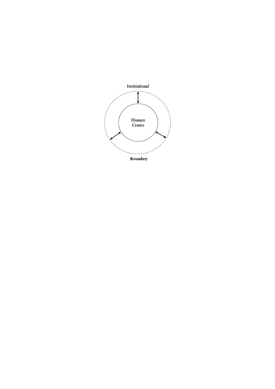
Figure 1.1

Human Center and Institutional Boundary

• The Institutional Boundary is society’s particular set of social

institutions that are each a conglomeration of interconnected
roles, or commonly held expectations about appropriate
behavior patterns. We define these roles independently of
whether or not the expectations they represent will continue
to be fulfilled, and apart from whatever incentives do or do not
exist for individuals to choose to behave in their accord. The
Institutional Boundary is necessary in any human society since
we are neither immortal nor omniscient, and is distinct from
both human consciousness and activity. It is human con-
sciousness that makes possible purposeful transformations of
the Institutional Boundary through human activity.

COMPLEMENTARY HOLISM

A social theory useful for pursuing human liberation must highlight
the relationship between social institutions and human characteris-
tics. But it is also important to distinguish between different areas,
or spheres of social life, and consider the possible relationships
between them. In Liberating Theory seven progressive authors called
our treatment of these issues “complementary holism.”

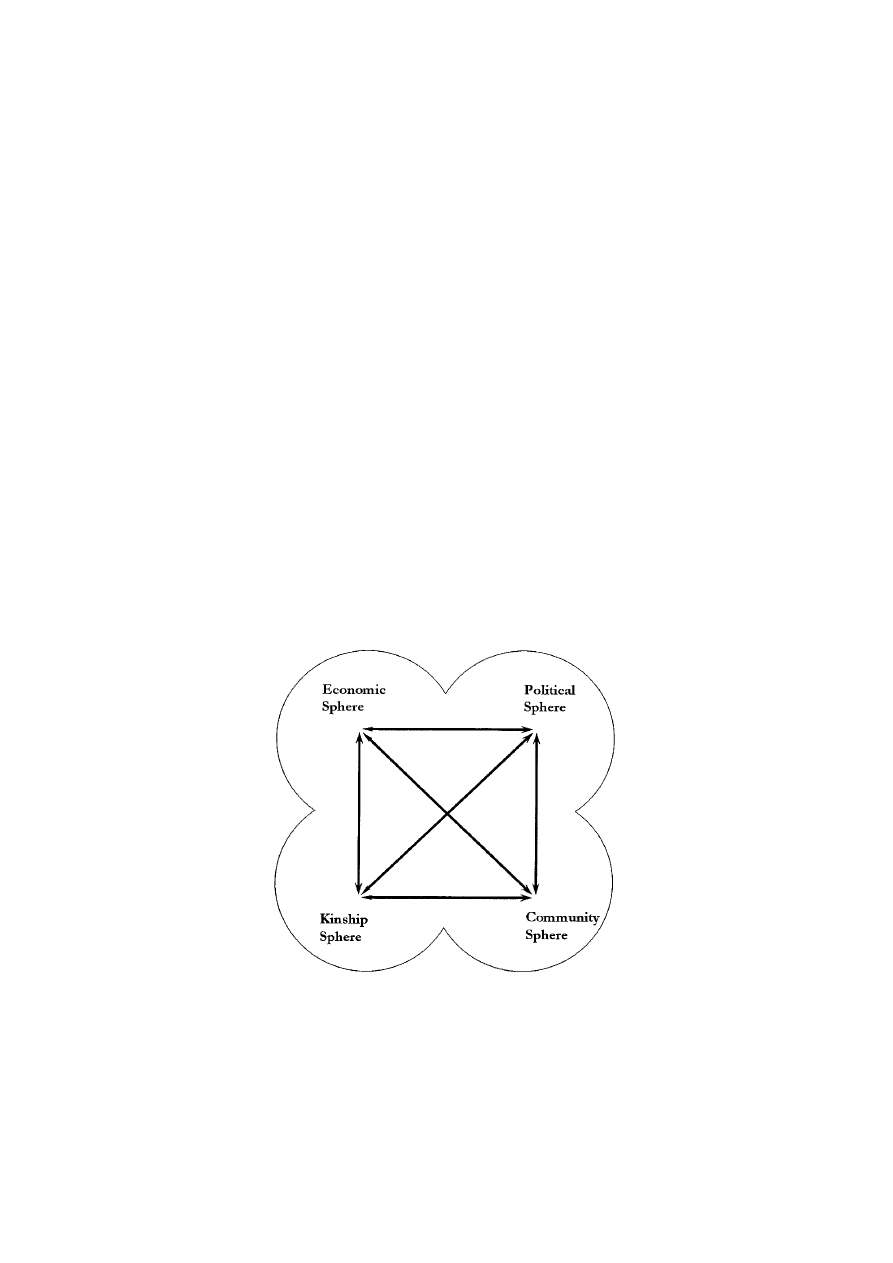
Four spheres of social life

The economy is not the only “sphere” of social activity. In addition
to creating economic institutions to organize our efforts to meet
material needs and desires, people have organized community insti-
tutions for addressing our cultural and spiritual needs, intricate
“sex-gender,” or “kinship” systems for satisfying our sexual needs
and discharging our parental functions, and elaborate political
systems for mediating social conflicts and enforcing social decisions.
So in addition to the economic sphere of social life we have what we
call a community sphere, a kinship sphere, and a political sphere as well.
In this book we will be primarily concerned with evaluating the per-
formance of the economic sphere, but the possible relationships
between the economy and other spheres of social life are worthy of
some consideration.

A monist paradigm presumes some form of dominance, or

hierarchy of influence among the spheres of social life, while a
pluralist social theory studies the dynamics of each sphere separately
and then attempts to sum the results. A complementary holist

Economics and Liberating Theory

approach assumes any form of dominance (or lack of dominance)
among the four spheres of social life is a matter to be determined by
empirical study of particular societies. All four spheres are socially
necessary. Any society that failed to produce and distribute the
material means of life would cease to exist. Some Marxists argue that
this implies that the economic sphere, or what they call the
economic “base” or “mode of production,” is necessarily dominant
in any and all human societies. But any society that failed to
procreate and rear the next generation would also cease to exist. So
the kinship sphere of social life is just as “socially necessary” as the
economic sphere. And any society that failed to mediate conflicts
among its members would disintegrate. Which means the political
sphere of social life is necessary as well. Finally, since all societies
have existed in the context of other, historically distinct societies,
and many contain more than one historically distinct community,
all societies have had to establish some kind of relations with other
social communities, and most have had to define relations among
internal communities as well. This means that the community
sphere of social life is as necessary as the political, kinship, and
economic spheres.

The ABCs of Political Economy

Figure 1.2

Four Spheres of Social Life

Besides being necessary, each of the four spheres is usually

governed by elaborate social institutions that can take many
different forms and have significant impacts on people’s character-
istics and behavior. This, more than their “social necessity” is why
complementary holism recognizes that all four spheres are
important, but that any pattern of dominance that may or may not
result cannot be determined by theory alone. Instead of a priori pre-
sumptions of dominance, complementary holism holds there are a
number of possible kinds of relations that can exist among spheres,
and which possibility pertains in a particular society can only be
determined by empirical investigation.

Relations between center, boundary and spheres

The human center andinstitutional boundary, andthe four spheres
of social life, are useful conceptual building blocks for an emancipa-
tory social theory. The concepts human center andinstitutional
boundary include all four kinds of social activity, but distinguish
between people andinstitutions. The spheres of social life encompass
both the human andinstitutional aspects of a particular kindof
social activity, but distinguish between different primary functions
of different activities. The possible relations between center and
boundary, and between different spheres, are obviously critical.

It is evident that if a society is to be stable people must generally

fit the roles they are going to fill. Actual behavior must generally
conform to the expected patterns of behavior defined by society’s
major social institutions. People must choose activities in accord
with the roles available, and this requires that people’s personalities,
skills, and consciousness be such that they do so. We must be capable
and willing to do what is required of us. In other words, there must
be conformity between society’s human center and institutional
boundary for social stability.

Suppose this were not the case. For example, suppose South

African whites had shed their racist consciousness overnight, but all
the institutions of apartheid had remained intact. Unless the insti-
tutions of apartheid were also changed, rationalization of continued
participation in institutions guided by racist norms would have
eventually regenerated racist consciousness among South African
whites. Or, on a smaller scale, suppose one professor eliminates
grades, makes papers optional, and no longer dictates course
curriculum nor delivers monologues for lectures, but instead, awaits
student initiatives. If students arrive conditioned to respond to

Economics and Liberating Theory

grading incentives alone, wanting to be led or entertained by the
instructor, then the elimination of authoritarianism in the institu-
tional structures of a single classroom in the context of continued
authoritarian expectations in the student body would result in very
little learning indeed.

Social stability and social change

Whether the result of any “discrepancy” between the human center
and institutional boundary will lead to a remolding of the center to
conform with an unchanged boundary, or changes in the boundary
that make it more compatible with the human center cannot be
known in advance. But in either case stabilizing forces within societies
act to bring the center and boundary into conformity, and lack of
conformity is a sign of social instability.

But this is not to say that the human centers and institutional

boundaries of all human societies are equally easy to stabilize. While
we are always being socialized by the institutions we confront, this
process can run into more or fewer obstacles depending on the
extent to which particular institutional structures are compatible or
incompatible with innate human potentials. In other words, just as
there are always stabilizing forces at work in societies, there are often
destabilizing forces as well resulting from institutional incompatibil-
ities with fundamental human needs. For example, no matter how
well oiled the socialization processes of a slave society, there remains
a fundamental incompatibility between the social role of slave and
the innate human potential and need for self-management. That
incompatibility is a constant source of potential instability in
societies that seek to confine people to slave status.

It is also possible for dynamics in one sphere to reinforce or desta-

bilize dynamics in another sphere of social life. For example, it might
be that the functioning of the nuclear family produces authoritar-
ian personality structures that reinforce authoritarian dynamics in
economic relations. Dynamics in economic hierarchies might also
reinforce patriarchal hierarchies in families. In this case authoritar-
ian dynamics in the economic and kinship spheres would be
mutually reinforcing. Or, hierarchies in one sphere sometimes
accommodate hierarchies in other spheres. For example, the
assignment of people to economic roles might accommodate
prevailing hierarchies in community and kinship spheres by placing
minorities and women into inferior economic positions. It is also
possible that role definitions themselves in a sphere are influenced

The ABCs of Political Economy

by dynamics from another sphere. For instance, if the economic role
of secretary includes tending the coffee machine as well as dictation,
typing, and filing, the role of secretary is defined not merely by
economic dynamics but by kinship dynamics as well.

On the other hand, it is possible for the activity in one sphere to

disrupt the manner in which activity is organized in another sphere.
For instance, the educational system as one component of the
kinship sphere might graduate more people seeking a particular kind
of economic role than the economic sphere can provide under its
current organization. This would produce destabilizing expectations
and demands in the economic sphere, and\or the educational
system in the kinship sphere. Some argued this was the case during
the 1960s and 1970s in the US when college education was expanded
greatly and produced “too many” with higher level thinking skills
for the number of positions permitting the exercise of such
potentials in the monopoly capitalist US economy – giving rise to a
“student movement.” In any case, at the broadest level, there can be
either stabilizing or destabilizing relations among spheres.

Agents of history

The stabilizing and destabilizing forces that exist between center and
boundary and among different spheres of social life operate
constantly whether or not people in the society are aware of them
or not. But these ever present forces for social stability or social
change are usually complemented by conscious efforts of particular
social groups seeking to maintain or transform the status quo.
Particular ways of organizing the economy may generate privileged
and disadvantaged classes. Similarly, the organization of kinship
activity may distribute the burdens and benefits unequally between
gender groups – for example granting men more of the benefits while
assigning them fewer of the burdens of kinship activity than women.
And particular community institutions may not serve the needs of
all community groups equally well, for example denying racial or
religious minorities rights or opportunities enjoyed by majority com-
munities. Therefore, besides underlying forces that stabilize or
destabilize societies, groups who enjoy more of the benefits and
shoulder fewer of the burdens of social cooperation in any sphere
have an interest in acting to preserve the status quo. Groups who
suffer more of the burdens and enjoy fewer of the benefits under
existing arrangements in any sphere can become agents for social
change. In this way groups that are either privileged or disadvan-

Economics and Liberating Theory

taged by the rules of engagement in any of the four spheres of social
life can become agents of history.

The key to understanding the importance of classes without

neglecting or underestimating the importance of privilegedanddis-
advantaged groups defined by community, kinship or political
relations is to recognize that only some agents of history are
economic groups, or classes. Racial, gender, and political groups can
also be conscious agents working to preserve or change the status
quo, which consists not only of the reigning economic relations, but
the dominant gender, community, and political relations as well.

Pre-Mandela South African society is a useful case to consider. Of
course the economy generatedprivilegedandexploitedclasses – cap-
italists andworkers, landowners andtenants, etc. South African
patriarchal gender relations also disadvantaged women compared to
men, andundemocratic political institutions empowereda minority
anddisenfranchisedmost citizens. But the most important social
relations, from which the system derived its name, apartheid, were
rules for classifying citizens into specific communities – whites,
colored, blacks – and defining different rights and obligations for
people according to their community status. The community
relations of apartheidcreatedoppressor andoppressedracial
community groups who playedthe principal roles in the social struggle
to preserve or overthrow the status quo in South Africa. This per-
spective need not deny that classes, or gender groups for that matter,
playedsignificant roles as well. But a social theory that recognizes all
spheres of social life, and understands that privileged and disad-
vantagedgroups can emerge from any of these areas where the
burdens and benefits of social cooperation are not distributed
equally, can help us avoidneglecting important agents of history,
andhelp us understandwhy not all forms of oppression will be
redressed by a social revolution in one sphere of social life alone –
as important as that change may be.

The ABCs of Political Economy

3. Broadly speaking the term “economism” means attributing greater

importance to the economy than is warranted. It can take the form of
assuming that dynamics in the economic sphere are more important than
dynamics in other spheres when this, in fact, is not the case in some
particular society. It can also take the form of assuming that classes are more
important agents of social change, and racial, gender or political groups
are less important “agents of history” than they actually are in a particular
situation.

Hopefully this conception of human beings, human societies, and

different spheres of social life in the liberating social theory
summarized in this chapter provides a proper setting for our study
of “political economy” – one that neither overstates nor understates
its role in the social sciences. In chapter 2 we proceed to think about
how to evaluate the performance of any economy.

Economics and Liberating Theory

What Should We Demand
from Our Economy?

It is easy enough to say we want an economy that distributes the
burdens and benefits of social labor fairly, that allows people to make
the decisions that affect their economic lives, that develops human
potentials for creativity, cooperation andempathy, andthat utilizes
human andnatural resources efficiently. It is also easy to say we want
“sustainable development.” But what does all this mean more
precisely?

ECONOMIC JUSTICE

Is it necessarily unfair when some work less or consume more than
others? Do those with more productive property deserve to work less
or consume more? Do those who are more talented or more educated
deserve more? Do those who contribute more, or those who make
greater sacrifices, or those who have greater needs deserve more? By
what logic are some unequal outcomes fair and others not?

Equity takes a back seat to efficiency for most mainstream

economists, while the issue of economic justice has long been a
passion of political economists. From Proudhon’s provocative quip
that “property is theft,” to Marx’s three volume indictment of
capitalism as a system based on the “exploitation of labor,”
economic justice and injustice has been a major theme in political
economy. After briefly reviewing evidence of rising economic
inequality within the United States and globally, we compare con-
servative, liberal and radical views of economic justice, and explain
why political economists condemn most of today’s growing inequal-
ities as escalating economic injustice.

Increasing inequality of wealth and income

As we begin the twenty-first century, escalating economic inequality
makes all other economic changes pale in comparison. The evidence

of increasing wealth and income inequality is overwhelming. In a
study published in 1995 by the Twentieth Century Fund, Edward
Wolff concludes:

Many people are aware that income inequality has increased over
the past twenty years. Upper-income groups have continued to do
well while others, particularly those without a college degree and
the young have seen their real income decline. The 1994 Economic
Report of the President refers to the 1979–1990 fall in real income of
men with only four years of high school – a 21% decline – as
stunning. But the growing divergence evident in income distrib-
ution is even starker in wealth distribution. Equalizing trends of
the 1930s–1970s reversed sharply in the 1980s. The gap between
haves and have-nots is greater now than at any time since 1929.

Chuck Collins and Felice Yeskel report: “In 1976, the wealthiest one
percent of the population owned just under 20% of all the private
wealth. By 1999, the richest 1 percent’s share had increased to over
40% of all wealth.” And they calculate that in the twenty-three years
between 1976 and 1999 while the top 1% of wealth holders doubled
their share of the wealth pie, the bottom 90% saw their share cut
almost in half.

Between 1983 and 1989 the average financial wealth

of households in the United States grew at an annual rate of 4.3%
after being adjusted for inflation. But the top 1% of wealth holders
captured an astounding 66.2% of the growth in financial wealth, the
next 19% of wealth holders captured 36.8%, and the bottom 80%
of wealth holders in the US lost 3.0% of their financial wealth. As a
result, the top 1% increased their share of total wealth in the US from
31% to 37% in those six years alone, and by 1989 the richest 1% of
families held 45% of all nonresidential real estate, 62% of all business
assets, 49% of all publicly held stock, and 78% of all bonds.

Moreover, “most wealth growth arose from the appreciation (or
capital gains) of pre-existing wealth and not savings out of income.
Over the 1962 to 1989 period, roughly three-quarters of new wealth

What Should We Demand from Our Economy?

1. Edward N. Wolff, Top Heavy: A Study of the Increasing Inequality of Wealth

in America (The Twentieth Century Fund, 1995): 1–2.

2. Chuck Collins and Felice Yeskel with United for a Fair Economy, Economic

Apartheid in America (The New Press, 2000): 54–7.

3. The New Field Guide to the US Economy, by Nancy Folbre and the Center for

Popular Economics (The New Press, 1995).

was generated by increasing the value of initial wealth – much of it
inherited.”

When we look to see who benefitted from the stock

market boom between 1989 and 1997 the same pattern emerges. The
top 1% of wealth holders captured an astonishing 42.5% of the stock
market gains over those years, the next 9% of wealth holders
captured an additional 43.3% of the gains, the next 10% captured
3.1%, while the bottom 80% of wealth holders captured only 11%
of the stock market gains.

While growing wealth inequality has been more dramatic, income

inequality has been growing as well. Real wages have fallen in the US
since the mid 1970s to where the average hourly wage adjusted for
inflation was lower in 1994 than it had been in 1968. Moreover, this
decline in real hourly wages has occurred despite continual increases
in labor productivity. Between 1973 and 1998 labor productivity
grew 33%. Collins and Yeskel calculate that if hourly wages had
grown at the same rate as labor productivity the average hourly wage
in 1998 would have been $18.10 rather than $12.77 – a difference of
$5.33 an hour, or more than $11,000 per year for a full-time worker.

Moreover, the failure of real wages to keep up with labor productiv-
ity growth has been worse for those in lower wage brackets. Between
1973 and 1993 workers earning in the 80th percentile gained 2.7%
in real wages while workers in the 60th percentile lost 4.9%, workers
in the 40th percentile lost 9.0%, and workers in the 20th percentile
lost 11.7% – creating much greater inequality of wage income.

In contrast, corporate profit rates in the US in 1996 reached their

highest level since these data were first collected in 1959. The Bureau
of Economic Analysis reported that the before-tax profit rate rose to
11.4% and the after-tax rate rose to 7.6% in 1996 – yielding an eight-
year period of dramatic, sustained increases in corporate profits the
Bureau called “unparalleled in US history.” Moreover, whereas
previous periods of high profits accompanied high rates of
investment and economic growth, the average rate of economic
growth over these eight years was just 1.9%. Whatever was good for
corporate profits was clearly not so good for the rest of us.

The ABCs of Political Economy

4. Lawrence Mishel and Jared Bernstein, The State of Working America

1994–1995 (ME Sharpe, 1994): 246.

5. The State of Working America 1998–1999: 271.
6. Economic Apartheid in America: 56.
7. The State of Working America 1994–1995: 121.

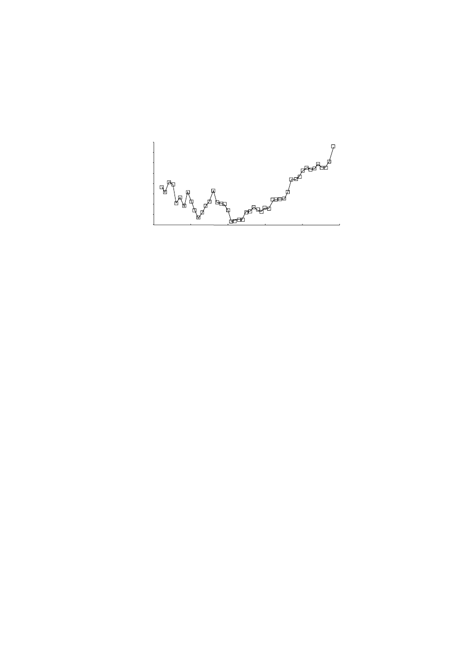
While there are a number of different ways to measure inequality,

the most widely used by economists is a statistic called the Gini coef-
ficient. A value of 0 corresponds to perfect equality and a value of 1
corresponds to perfect inequality. Figure 2.1 plots the Gini coeffi-
cient for household income in the United States from 1947 to 1993.
The steady increase in the Gini coefficient from a low of 0.405 in
1966 to a high of 0.479 in 1993 represents a remarkable, and his-
torically unprecedented 18.3% increase in income inequality among
US households over the time period.

Trends in global inequality are equally, if not more disturbing.

Walter Park and David Brat report in a study of gross domestic
product per capita in 91 countries that the value of the Gini rose
steadily from 0.442 in 1960 to 0.499 in 1988. In other words,
between 1960 and 1988 there was an increase in the economic
inequality between countries of 13%.

All evidence available so far

confirms that this trend continued in the 1990s and first two years
of the new millennium as neoliberal globalization accelerated.

The facts are clear: We are experiencing increases in economic

inequality inside the US reminiscent of the “Robber Baron era” of
US capitalism over a hundred years ago, and global inequality is
accelerating at an unprecedented pace. But how should we interpret

What Should We Demand from Our Economy?

1945

1955

1965

1975

1985

1995

0.48

0.47

0.46

0.45

0.44

0.43

0.42

0.41

0.40

Year

Gini Coefficient

Figure 2.1

Gini Coefficients for US Household Income 1947–93

8. Source: Edward Wolff, Economics of Poverty, Inequality and Discrimination

(South-Western Publishing, 1997): 75.

9. Walter Park and David Brat, “A Global Kuznets Curve?” Kylos, Vol. 48,

1995: 110.

the facts? When are unequal outcomes inequitable and when are
they not?

Different conceptions of economic justice

What is an equitable distribution of the burdens and benefits of
economic activity? Philosophers, economists, and political scientists
have offered three different distributive maxims attempting to
capture the essence of economic justice, which we can label the con-
servative, liberal, and radical definitions of economic justice.

Conservative Maxim 1: Payment according to the value of one’s
personal contribution and the contribution of the productive property one
owns.

The rationale behind the conservative maxim is that people should
get out of an economy what they and their productive possessions
contribute to the economy. If we think of the goods and services, or
benefits of an economy, as a giant pot of stew, the idea is that indi-
viduals contribute to how big and rich the stew will be by their labor
and by the productive assets they bring to the kitchen. If my labor
and productive assets make the stew bigger or richer than your labor
and assets, then according to maxim 1 it is only fair that I eat more
stew, or richer morsels, than you do.

While this rationale has obvious appeal, it has a major problem I

call the Rockefeller grandson problem. According to maxim 1 the
grandson of a Rockefeller with a large inheritance of productive
property should eat 1000 times as much stew as a highly trained,
highly productive, hard working son of a pauper – even if Rocke-
feller’s grandson doesn’t work a day in his life and the pauper’s son
works for fifty years producing goods or providing services of great
benefit to others. This will inevitably occur if we count the contri-
bution of productive property people own, and if people own
different amounts of machinery and land, or what is the same thing,
different amounts of stocks in corporations that own the machinery
and land, since bringing a cooking pot or stove to the economy
“kitchen” increases the size and quality of the stew we can make just
as surely as peeling more potatoes and stirring the pot more does.
So anyone who considers it unfair when the idle grandson of a Rock-
efeller consumes more than a hard working, productive son of a
pauper cannot accept maxim 1 as the definition of equity.

The ABCs of Political Economy

A second line of defense for the conservative maxim is based on

a vision of “free and independent” people, each with his or her own
property, who, it is argued, would refuse to voluntarily enter a social
contract on any other terms. This view is commonly associated with
the writings of John Locke. But while it is clear why those with a
great deal of productive property in Locke’s “state of nature” would
have reason to hold out for a social contract along the lines of
maxim 1, why would not those who wander the state of nature with
little or no productive property in their backpacks hold out for a very
different arrangement? If those with considerable wherewithal can
do quite well for themselves in the state of nature, whereas those
without cannot, it is not difficult to see how requiring unanimity
would drive the bargain in the direction of maxim 1. But then
maxim 1 is the result of an unfair bargaining situation in which the
rich are better able to tolerate failure to reach an agreement over a
fair way to assign the burdens and benefits of economic cooperation
than the poor, giving the rich the upper hand in negotiations over
the terms of the social contract. In this case the social contract
rationale for maxim 1 loses moral force because it results from an
unfair bargain.

This suggests that unless those with more productive property

acquired it through some greater merit on their part, the income
they accrue from this property is unjustifiable, at least on equity
grounds. That is, while the unequal outcome might be desirable for
some other reason such as improving economic efficiency, it would
not be just or fair. In which case maxim 1 must be rejected as a
definition of equity if we find that those who own more productive
property did not come by it through greater merit. One way people
acquire productive property is through inheritance. But it is difficult
to see how those who inherit wealth are more deserving than those
who don’t. It is possible the person making a bequest worked harder
or consumed less than others in her generation, and in one of these
ways sacrificed more than others. Or it is possible the person making
the bequest was more productive than others. And we might decide
that greater sacrifice or greater contribution merits greater reward.
But in these scenarios it is not the heir who made the greater sacrifice
or contribution, it is the person who made the bequest, so the heir
would not deserve greater wealth on those grounds. As a matter of
fact, if we decide rewards are earned by sacrifice or personal contri-
bution, inherited wealth violates either norm since inheriting wealth
is neither a sacrifice nor a personal contribution. A more compelling

What Should We Demand from Our Economy?

argument for inheritance is that banning inheritance is unfair to
those wishing to make bequests rather than that it is unfair to those
who would receive them. One could argue that if wealth is justly
acquired it is wrong to prevent anyone from disposing of it as they
wish – including bequeathing it to their descendants. However, it
should be noted that any “right” of wealthy members of older gen-
erations to bequeath their gains to their offspring would have to be
weighed against the “right” of people in younger generations to start
with “equal economic opportunities.”

Indeed, these two “rights”

are obviously in conflict, and some means of adjudicating between
them is required. But no matter how this matter is settled, it appears
that those who receive income from inherited wealth benefit from
an unfair advantage.

A second way people acquire more productive property than

others is through good luck. Working or investing in a rising or
declining company or industry constitutes good luck or bad luck.
But unequal distributions of productive property that result from dif-
ferences in luck are not the result of unequal sacrifices, unequal
contributions, or any difference in merit between people. Luck, by
its very definition is not deserved, and therefore the unequal
incomes that result from unequal distributions of productive
property due to differences in luck appear to be inequitable as well.

A third way people come to have more productive property is

through unfair advantage. Those who are stronger, better connected,
have inside information, or are more willing to prey on the misery
of others can acquire more productive property through legal and
illegal means. Obviously if unequal wealth is the result of someone
taking unfair advantage of another it is inequitable.

The last way people might come to have more productive property

than others is by using some income they earned fairly to purchase
more productive property than others can. What constitutes fairly
earned income is the subject of maxims 2 and 3 which are discussed
below. But there is a difficult moral issue regarding income from
productive property even if the productive property was purchased
with income we stipulate was fairly earned in the first place. In
chapter 3 we will discover that labor and credit markets allow people

The ABCs of Political Economy

10. We are not talking about willing personal belongings to decedents, which

is unobjectionable, but passing on productive property in quantities
that significantly skew the economic opportunities of members of the
new generation.

with productive wealth to capture part of the increase in productiv-
ity of other people that results when other people work with the
productive wealth. Whether or not, and to what extent, the profit or
rent which owners of productive wealth initially receive is merited
we will examine very carefully. But even if we stipulate that some
compensation is justified by a meritorious action that occurred once
in the past, it turns out that labor and credit markets allow those
who own productive wealth to parlay it into permanently higher
incomes which increase over time with no further meritorious
behavior on their parts. This creates the dilemma that ownership of
productive property even if justly acquired may well give rise to
additional income that, while fair initially, becomes unfair after
some point, and increasingly so. The simple corn model we explore
in chapter 3 illustrates this moral dilemma nicely.

In sum, if unequal accumulations of productive property were the

result only of meritorious actions, and if compensation ceased when
the social debt was fully repaid, using words like “exploitation” to
describe payments to owners of productive property would seem
harsh and misleading. On the other hand, if those who own more
productive property acquired it through inheritance, luck, unfair
advantage – or because once they have more productive property
than others they can accumulate even more with no further above-
average meritorious behavior through labor or credit markets – then
calling the unequal outcomes that result from differences in wealth
unfair or exploitative seems perfectly appropriate. Most political
economists believe a compelling case can be made that differences
in ownership of productive property which accumulate within a
single generation due to unequal sacrifices and/or unequal contri-
butions people make themselves are small compared to the
differences in wealth that develop due to inheritance, luck, unfair
advantage, and accumulation. Edward Bellamy put it this way in
Looking Backward written at the end of the nineteenth century: “You
may set it down as a rule that the rich, the possessors of great wealth,
had no moral right to it as based upon desert, for either their
fortunes belonged to the class of inherited wealth, or else, when
accumulated in a lifetime, necessarily represented chiefly the
product of others, more or less forcibly or fraudulently obtained.”
One hundred years later Lester Thurow estimated that between 50
and 70% of all wealth in the US is inherited. Daphne Greenwood
and Edward Wolff estimated that 50 to 70% of the wealth of
households under age 50 was inherited. Laurence Kotlikoff and

What Should We Demand from Our Economy?

Lawrence Summers estimated that as much as 80% of personal
wealth came either from direct inheritance or the income on
inherited wealth.

A study published by United for a Fair Economy

in 1997 titled “Born on Third Base” found that of the 400 on the
1997 Forbes list of wealthiest individuals and families in the US, 42%
inherited their way onto the list; another 6% inherited wealth in
excess of $50 million, and another 7% started life with at least $1
million. In any case, presumably what Proudhon was thinking when
he coined the phrase “property is theft” was that most large wealth
holders acquire their wealth through inheritance, luck, unfair
advantage, or unfair accumulation. A less flamboyant radical might
have stipulated that he was referring to productive, not personal
property, and added the qualification “property is theft – more often
than not.”

Liberal Maxim 2: Payment according to the value of one’s personal con-
tribution only.

While those who support the liberal maxim find most property
income unjustifiable, advocates of maxim 2 hold that all have a right
to the “fruits of their own labor.” The rationale for this has a
powerful appeal: If my labor contributes more to the social endeavor
it is only right that I receive more. Not only am I not exploiting
others, they would be exploiting me by paying me less than the
value of my personal contribution. But ironically, the same reason
for rejecting the conservative maxim applies to the liberal maxim as
well.

Economists define the value of the contribution of any input in

production as the “marginal revenue product” of that input. In other
words, if we add one more unit of the input in question to all of the
inputs currently usedin a production process, how much wouldthe
value of output increase? The answer is defined as the marginal
revenue product of the input in question. But mainstream economics
teaches us that the marginal productivity, or contribution of an

The ABCs of Political Economy

11. Lester Thurow, The Future of Capitalism: How Today’s Economic Forces Will

Shape the Future (William Morrow, 1996), Daphne Greenwood and Edward
Wolff, “Changes in Wealth in the United States 1962–1983,” Journal of
Population Economics 5, 1992, and Laurence Kotlikoff and Lawrence
Summers, “The Role of Intergenerational Transfers in Aggregate Capital
Accumulation,” Journal of Political Economy 89, 1981.

input, depends as much on the number of units of that input
available, andon the quantity andquality of other, complimentary
inputs, as on any intrinsic quality of the input itself – which
undermines the moral imperative behind any “contribution based”
maxim – that is, maxim 2 as well as maxim 1. But besides the fact
that the marginal productivity of different kinds of labor depends
mostly on the number of people in each labor category in the first
place, andon the quantity andquality of non-labor inputs available
for them to use, most of the remaining differences in people’s
personal productivities are due to personal differences beyond
people’s control which cannot be tracedto differential sacrifices. No
amount of eating and weight lifting will give an average individual
a 6 feet 11 inches frame with 350 plus pounds of muscle. Yet profes-
sional football players in the United States receive hundreds of times
more than an average salary because those attributes make their con-
tribution outrageously high in the context of US sports culture. The
famous British political economist, Joan Robinson, pointedout long
ago, that however “productive” a machine or piece of land may be,
that hardly constitutes a moral argument for paying anything to its
owner. In a similar vein one couldargue that however “productive”
a high IQ or a 350 poundphysique may be, that doesn’t mean the
owner of this trait deserves more income than someone less gifted
who works as hardandsacrifices as much. The bottom line is that
the “genetic lottery” greatly influences how valuable a person’s con-
tribution will be. Yet the genetic lottery is no more fair than the
inheritance lottery – which implies that as a conception of economic
justice maxim 2 suffers from a similar flaw as maxim 1.

In defense of maxim 2 it is frequently argued that while talent

may not deserve reward, talent requires training, and herein lies the
sacrifice that merits reward: Doctor’s salaries are compensation for
all the extra years of education. But longer training does not neces-
sarily mean greater personal sacrifice. It is important not to confuse
the cost of someone’s training to society – which consists mostly of

What Should We Demand from Our Economy?

12. Milton Friedman argued this point eloquently in Capitalism and Freedom

(University of Chicago Press, 1964): chapter 10. However, his conclusion
was that since maxim 2 cannot be defended on moral grounds, critics of
capitalism, which distributes the burdens and benefits of economic coop-
eration according to maxim 1, should mute their criticisms. Essentially
Friedman reminded critics of capitalism who favor maxim 2 over maxim
1 that those who live in glass houses shouldn’t throw stones!

the trainer’s time and energy, and scarce social resources like books,
computers, libraries, and classrooms – with the personal sacrifice of
the trainee. If teachers and educational facilities are paid for at public
expense – that is, if we have a universal public education system –
and if students are paid a living stipend – so they forego no income
while in school – then the personal sacrifice of the student consists
only of their discomfort from time spent in school. But even the
personal suffering we endure as students must be properly compared.
While many educational programs are less personally enjoyable than
time spent in leisure, comparing discomfort during school with
comfort during leisure is not the relevant comparison. The relevant
comparison is with the discomfort others experience who are
working instead of going to school. If our criterion is greater personal
sacrifice than others, then logic requires comparing the student’s
discomfort to whatever level of discomfort others are experiencing
who work while the student is in school. Only if schooling is more
disagreeable than working does it constitute a greater sacrifice than
others make, and thereby deserves reward. So to the extent that
education is born at public rather than private expense, and the
personal discomfort of schooling is no greater than the discomfort
others incur while working, extra schooling merits no compensation
on moral grounds.

In sum, I call the problem with maxim 2 the “doctor–garbage

collector problem.” If education were free all the way through medical
school, how could it be fair to pay a brain surgeon who is on the first
tee at his country club golf course by 1 p.m. even on the four days a
week he works, ten times more than a garbage collector who works
under miserable conditions 40 plus hours a week.

Radical Maxim 3: Payment according to effort, or the personal sacrifices
one makes.

Which brings us to radical maxim 3. Whereas differences in contri-
bution will be due to differences in talent, training, job assignment,
luck, and effort, the only factor that deserves extra compensation
according to maxim 3 is extra effort. By “effort” is meant personal
sacrifice for the sake of the social endeavor. Of course effort can take
many forms. It may be longer work hours, less pleasant work, or
more intense, dangerous, unhealthy work. Or, it may consist of
undergoing training that is less gratifying than the training experi-
ences of others, or less pleasant than time others spend working who

The ABCs of Political Economy

train less. The underlying rationale for maxim 3 is that people should
eat from the stew pot according to the sacrifices they made to cook
it. According to maxim 3 no other consideration, besides differential
sacrifice, can justify one person eating more stew than another.

Even for those who reject contribution-based theories of economic

justice like maxims 1 and 2 as inherently flawed because people’s
abilities to contribute are different through no fault of their own,
there is still a problem with maxim 3 from a moral point of view
that I call the “AIDS victim problem.” Suppose someone has made
average sacrifices for 15 years, and consumed an average amount.
Suddenly they contract AIDS through no fault of their own. In the
early 1990s a medical treatment program for an AIDS victim often
cost close to a million dollars. That is, the cost to society of providing
humane care for an AIDS victim was roughly a million dollars. If we
limit people’s consumption to the level warranted by their efforts,
we would have to deny AIDS victims humane treatment, which
many would find hard to defend on moral grounds.

Of course this is where another maxim comes to mind: payment

according to need. Whether taking differences in need into consider-
ation is required by economic justice or is required, instead, for an
economy to be humane is debatable. In my personal view the
humane maxim, payment according to need, is in a different
category than the other three and expresses a commendable value,
but a value beyond economic justice. It seems to me that it is one
thing for an economy to be an equitable economy – one that is fair
and just. It is another thing for an economy also to be humane.
While I believe justice requires compensating people according to
the sacrifices they make, it seems to me that it is our humanity that
compels us to provide for those in need. When considered in this
light a just economy is not the last word in morally desirable
economies. A just economy that allowed AIDs victims to suffer for
lack of proper medical care would, indeed, be morally deficient
because it would be inhumane. If thought of in this way, besides
striving for economic justice, we must work for a humane economy
as well, which entails distribution according to effort or sacrifice,
tempered by need.

EFFICIENCY

As long as resources are scarce relative to human needs and socially
useful labor is burdensome, in part, efficiency is preferable to waste-

What Should We Demand from Our Economy?

fulness. Political economists do not have to imitate our mainstream
colleagues and concentrate on efficiency to the detriment of other
important criteria such as economic justice and democracy in order
to recognize that people have every reason to be resentful if their
sacrifices are wasted or if limited resources are squandered.

The Pareto Principle

Economists usually define economic efficiency as Pareto optimality
– named after the late nineteenth-century Italian economist
Wilfredo Pareto. A Pareto optimal outcome is one where it is
impossible to make anyone better off without making someone else worse
off. The idea is simply that it would be inefficient or wasteful not to
implement a change that made someone better off and nobody worse off.
Such a change is called a Pareto improvement, and another way to
define a Pareto optimal, or efficient outcome, is an outcome where
there are no further Pareto improvements possible.

This does not mean a Pareto optimal outcome is necessarily

wonderful. If I have 10 units of happiness and you have 1, and there
is no way for me to have more than 10 unless you have less than 1,
and no way for you to have more than 1 unless I have fewer than 10,
then me having 10 units of happiness and you having 1 is a Pareto
optimal outcome. But you would be right not to regard it very
highly, and being a reasonable person, I would even agree with you.
Moreover, there are usually many Pareto optimal outcomes. For
instance, if I have 7 units of happiness and you have 6, and if there
is no way for me to have more than 7 unless you have fewer than 6,
and no way for you to have more than 6 unless I have fewer than 7,
then me having 7 and you having 6 is also a Pareto optimal
outcome. And we might both regard this second Pareto optimal
outcome as better than the first, even though I am personally better
off under the first. So the point is not that being in a Pareto optimal
situation is necessarily wonderful – that depends on which Pareto
optimal situation we’re in. Instead the point is that non-Pareto
optimal outcomes are clearly undesirable because we could make
someone better off without making anyone worse off – and it is
“inefficient” or wasteful not to do that. In other words, there is
something wrong with an economy that systematically yields non-
Pareto optimal outcomes, i.e., fails to make some of its participants
better off when doing so would make nobody worse off.

It is important to recognize that the Pareto criterion, or definition

of efficiency, is not going to settle most of the important economic

The ABCs of Political Economy

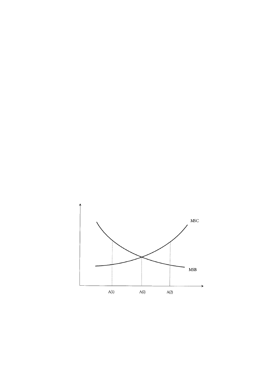
issues we face. Most policy choices will make some people better off
but others worse off, and in these situations the Pareto criterion has
nothing to tell us. Consequently, if economists confine themselves
to the narrow concept of efficiency as Pareto optimality, and only
recommend policies that are, in fact, Pareto improvements, we
would be rendered silent on most issues! For example, reducing
greenhouse gas emissions makes a lot of sense because the future
benefits of stopping global warming and avoiding dramatic climate
change far outweigh the present costs of reducing emissions. But
since a relatively few people in the present generation will be made
somewhat worse off no matter how we go about it, the fact that
many more people in future generations will be much better off does
not allow us to recommend the policy as a Pareto improvement –
that is, on efficiency grounds in the narrow sense.

The efficiency critierion

The usual way around this problem is to broaden the notion of
efficiency from Pareto improvements to changes where the benefits
to some outweigh the costs to others. This broader notion of
efficiency is called the efficiency criterion and serves as the basis for
cost benefit analysis. Simply put, the efficiency criterion says if the

What Should We Demand from Our Economy?

Figure 2.2

The Efficiency Criterion

overall benefits to any and all people of doing something outweigh the
overall costs to any and all people, it is “efficient” to do it. Whereas, if the
overall costs outweigh the overall benefits of doing something it is “ineffi-
cient” to do it.

We can illustrate the efficiency criterion using a very useful graph.

Suppose we knew the cost to society of growing each and every
apple. That is, suppose we knew how much of society’s scarce land,
labor, fertilizer, etc. it took to grow each and every apple, and we also
knew how much pesticide it took, and how much it “cost” society
when more pesticide seeped into our ground water, etc. We call this
the “Social Cost” of producing apples, and we call the Social Cost of
the last (or next) apple produced the Marginal Social Cost of apples,
or MSC for short. Suppose we also knew the benefit to society of
having another apple available to consume. The Social Benefit of the
last (or next) apple consumed is called the Marginal Social Benefit
of apples, or MSB for short. Now let us assume that the more apples
we have consumed already the less beneficial an additional apple
will be, and the more apples we have produced already the more it
costs society to produce another one. In this case if we plot the
number of apples on the horizontal axis and measure the Marginal
Social Benefit and Marginal Social Cost of apples on the vertical axis,
the MSB curve will be downward sloping and the MSC curve will be
upward sloping as it is in Figure 2.2. What is incredibly useful about
this diagram is it allows us to determine how many apples we should
produce and consume, i.e. the socially efficient or “optimal”
quantity of apples to produce, A(0). It is the amount where the
marginal social cost of producing the last apple, MSC, is equal to the
marginal social benefit from consuming the last apple, MSB. We can
demonstrate that the socially efficient, or optimal level of apple
production and consumption is the level below where the MSC and
MSB curves cross by showing that any lower or higher level of
production and consumption allows for an increase in net social
benefits and therefore violates the efficiency criterion.

Suppose someone thought we should produce fewer apples than

the level where MSC equals MSB, such as A(1) < A(0). For any level
of production less than A(0), such as A(1), what would be the effect
of producing one more apple than we are already producing? To see
what the additional cost to society would be, we go up from A(1) to
the MSC curve. To see what the additional benefit to society would
be we go up from A(1) to the MSB curve. But when we produce and
consume at A(1) the MSB curve is higher than the MSC curve,

The ABCs of Political Economy

indicating that producing and consuming another apple increases
social benefits more than it increases social costs. In other words, at
A(1) there would be positive net social benefits from expanding
production and consumption of apples.

Suppose someone thought we should produce more apples than

the level where MSC equals MSB, such as A(2) > A(0). For any level
of production greater than A(0), such as A(2), what would be the
effect of producing one apple less than we are already producing? To
see what the savings in social cost would be we go up from A(2) to
the MSC curve. To see what the lost social benefit would be we go up
from A(2) to the MSB curve. But when we produce and consume at
A(2) the MSC curve is higher than the MSB curve indicating that
producing and consuming one apple less reduces social benefits by
less than it reduces social costs. In other words, at A(2) there are
potential positive net social benefits from reducing production and
consumption of apples.

The conclusion is for all A < A(0) we should expand apple

production (and consumption), and for all A > A(0) we should reduce
apple production (and consumption.) Therefore the only level of
apple production that is efficient from society’s point of view is the
level where the Marginal Social Benefit of the last apple consumed
is equal to the Marginal Social Cost of the last apple produced, A(0).
In any other case we could increase net social benefits by expanding
or reducing apple production and consumption.

Mainstream economists do not like to admit that policies recom-

mended on the basis of the efficiency criterion are usually not Pareto
improvements since they do make some people worse off. The
efficiency criterion andall cost benefit analysis necessarily (1)
“compares” different people’s levels of satisfaction, and (2) attaches
“weights” to how important the satisfactions of different people are
when we calculate overall, or social benefits and social costs. Notice
that when I stipulatedthat a few wouldbe worse off in the present
generation if we reduce greenhouse gas emissions while many will
be benefittedin the future I was attributing greater weight to the
gains of the many in the future than the loses of a few in the
present. I think it is perfectly reasonable to do this, and do not
hesitate to do so. But I am attaching weights to the well being of
different people – in this case roughly equal weights, which I also
believe is reasonable. If one refuses to attach weights to the well
beings of different people the efficiency criterion cannot be used. I
also stipulatedthat the benefits of preventing global warming to

What Should We Demand from Our Economy?

people in the future were large comparedto the cost of reducing
emissions to people in the present. I was willing to compare how
large a gain was for one person comparedto how small a loss was for
a different person. If one refuses to compare the size of benefits and
costs to different people, the efficiency criterion cannot be used.
Unlike the narrow Pareto principle, the efficiency criterion requires
comparing the magnitudes of costs and benefits to different people
and deciding how much importance to attach to the well being of
different people.

In other words, the efficiency criterion requires value judgments

beyond what are required by the Pareto principle. So when
mainstream economists pretend they have imposed no value
judgments, and have separated efficiency from equity issues when
they apply cost benefit analysis and recommend policy based on the
efficiency criterion they misrepresent themselves. While a Pareto
improvement makes some better off at the expense of none – and
therefore does not require comparing the sizes of gains and losses to
different people or weighing the importance of well being to
different people – policies that satisfy the efficiency criterion
generally make some better off precisely at the expense of others,
which necessarily requires comparing the magnitudes of costs and
benefits to different people and making a value judgment regarding
how important the interests of the “winners” are compared to the
interests of the “losers.” Mainstream economists like to point out
that if a policy passes the efficiency criterion that means the
magnitude of benefits enjoyed by the winners is necessarily larger
than the magnitude of costs suffered by the losers, which means it
would be theoretically possible for the winners to fully compensate
the losers and still be better off themselves. But first, this requires a
comparison of the magnitude of gains to some compared to the
magnitude of losses to others – already a large step beyond the
narrow conceptualization of efficiency enshrined in the Pareto
principle that does not permit comparing different people’s satis-
factions. Secondly, either compensation is paid, or it is not paid. If
a policy requires winners to fully compensate losers then it is a Pareto
improvement and we do not need the broader efficiency criterion
to recommend it. If, on the other hand, a policy does not require
that losers be fully compensated from the gains to winners, then it
requires a value judgment that those who win deserve to do so, and
those who lose deserve to do so, before it can be recommended –
however much economists who claim to forswear “value judgments”

The ABCs of Political Economy

may wish otherwise. In the end, the only reason we need the
efficiency criterion in the first place is precisely because so many
important choices fall outside the purview of the Pareto principle,
i.e. cannot be reduced to efficiency defined narrowly.

Seven deadly sins of inefficiency

How might an economy be wasteful in the sense that it fails to
achieve a Pareto optimal outcome? It turns out there are seven
different ways that any economy might be inefficient. I facetiously
call them the seven “deadly sins” of inefficiency.

The production sector of an economy will be inefficient if:

1. It leaves productive resources idle. (Example: unemployed

workers, or idle crop land.)

2. It uses inefficient technologies, that is, uses more of some input

than necessary to get a given amount of output. (Example: The
same number of shoes can be made with less leather by more
careful cutting.)

3. It misallocates productive resources so that swapping inputs

between two different production units would lead to increases
in output in both. (Example: Assigning carpenters to a farm and
agronomists to the construction industry.)

The consumption sector will be inefficient if:

4. There are undistributed, or idle consumption goods. (Example:

Wheat rotting in silos while people go hungry.)

5. Final goods are misdistributed so that two or more consumers

could exchange goods and both be better off than under the
original distribution. (Examples: Apples are distributed to orange
lovers while oranges are distributed to apple lovers.)

And the production and consumption sectors will be inefficiently
integrated if:

6. Goods are misallocated between consumers and producers so it

is possible for a producer and consumer to swap goods and have
the output of the producer rise and the satisfaction of the
consumer increase as well. (Example: Personal computers are dis-
tributed to households that suffer for lack of heat while

What Should We Demand from Our Economy?

employees at accounting firms are unproductive in overheated
offices without personal computers to work with.)

7. Resources are misallocated to different industries so it is possible

to shift productive resources from one industry to another to
produce a different mixture of outputs more to consumers’ tastes.
(Example: Most land suitable for orchards is planted in pear trees
even though most consumers prefer apples to pears.)

The seven deadly sins of inefficiency provide an orderly, and not
overly intimidating, procedure for checking to see if an economy
will be inefficient in the narrow sense of the Pareto principle. All we
need to do is check if the economy is prone to “sinning” in any of
these seven ways. If not, we can conclude the economy is efficient,
or will achieve Pareto optimality, whatever other desirable or unde-
sirable qualities it may posess. Moreover, if the economy is prone to
inefficiency we will know what kind of inefficiency it suffers from.

Endogenous preferences

There is an important issue traditional treatments ignore which com-
plicates how we should think about efficiency. When people make
choices in light of their present preferences, the actions they take
not only fulfill their present preferences (to a greater or lesser degree),
they also change people’s human characteristics to some extent, and
thereby change their future needs and desires. In chapter 1 we saw
this is what it means to say people have “consciousness” and are
“self-creative.” While traditional treatments of efficiency take
account of the first effect of people’s choices – the “preference ful-
fillment effect” – the second effect – the “preference development
effect” – is usually ignored even though evaluating the effect of
economic choices and institutions on people’s human development
patterns may be as important as evaluating how well those choices
and institutions succeed in fulfilling their present preferences.
However, when economic choices have human development effects
that means they also change people’s preferences, creating the
following dilemma: How are we to judge the efficiency of economic
institutions using people’s preferences as our yardstick if those pref-
erences are in part a product of those same economic institutions in
the first place? While this may appear to be a vicious circle giving
rise to a philosophical conundrum that cannot be resolved, it turns
out there are some conclusions we can draw about economic
efficiency even when we recognize that people’s preferences are

The ABCs of Political Economy

influenced by the economic institutions that purport to satisfy those
preferences.

The view that people are self-conscious agents whose characteris-

tics and therefore preferences develop can be summarized in a model
of “endogenous preferences.” Using such a model it is possible to
demonstrate that if an economy is biased against a certain kind of
activity – that is, if people must pay more than the true cost to
society to engage in the activity:

1. The degree of inefficiency in the economy will be greater than

recognized by traditional theory that fails to treat preferences as
endogenous, and the inefficiency will increase, or “snowball”
over time.

2. Individual human development patterns will be “warped” in the

sense that they will not develop in ways that would generate the
most fulfillment people could enjoy, and the warping will
increase or “snowball” over time.

3. These detrimental, non-traditional effects of the bias in the

economy will be disguised to participants who adjust uncon-
sciously, or forget they have adjusted after the fact.

The intuition behind these political economy welfare theorems

that to the extent people recognize the “preference development”
as well as the “preference fulfillment” effects of their choices, it is
sensible for them to take both effects into account when making
decisions. If an economic institution is biased against some activity
– charging people more than the true social cost of their engaging in
the activity – then rational people will choose activities in part to
develop a lower preference for that activity than if they were only
charged the true social cost for engaging in it. It follows that the
demand for the activity in the future will be less than had people
not adjusted their preferences. But this reduced demand implies that
even fewer resources will be allocated to supplying the activity than
had people not adjusted their preferences. The more time people
have to make these individually rational adjustments, the lower
demand, and therefore supply of the activity will be, leading to ever
greater misallocations of productive resources as time goes on, and

What Should We Demand from Our Economy?

13. For a rigorous derivation of these results see chapter 6 in Robin Hahnel

and Michael Albert, Quiet Revolution in Welfare Economics (Princeton
University Press, 1990).

ever greater deviations of people’s human development trajectories
from those that would have maximized their well being under a
system of unbiased prices. If after the fact people forget that they
adjusted their preferences in response to the bias, they will only see
themselves as getting what they want.

In other words, if an economic institution introduces a bias in the

terms of availability of an activity, the consequence will be a “snow-
balling” divergence from efficient allocations. This implies that a
major criterion for judging economic institutions should be determining
whether they exert any systematic biases on individual choice, because to
the extent that people’s preferences are endogenous, any biases will
be more detrimental than traditionally recognized.

While traditional economists limit their evaluations of economies

to efficiency (without considering the complication of endogenous
preferences) and equity (about which they have little to say),
political economists have good reason to take other criteria into
account as well. Specifically, how and by whom decisions are made,
and the social effects of economic activities are important to evaluate
and take into account.

SELF-MANAGEMENT

I define self-management as decision making input in proportion to the
degree one is affected, and believe more self-management is desirable,
all other things being equal, or as economists like to say, ceteris
paribus.

The first thing to notice is that defined in this way self-

management is seldom equivalent either to individual freedom or
majority rule. Only if a single individual were the only person
affected by a decision would self-management be the same as
individual freedom, i.e. the right of a single individual to decide
whatever she pleases. And only if all were equally affected by a
decision would self-management be the same as majority rule, i.e.
one person one vote. Since most economic decisions affect more
than one person, but affect people to different degrees, self-
management as I have defined it usually requires that some people
have more decision making power while others have less regarding
any particular economic decision.

But why is more self-management a good thing? Throughout

history most humans have lived in circumstances with few oppor-
tunities for economic self-management. So admittedly, most people

The ABCs of Political Economy

don’t die without it. Political economists contend that just as denial
of material means of subsistence conflicts with human “natural”
needs for food, shelter, and clothing, denial of self-management
opportunities is in conflict with our “species nature.” The capacity
to analyze and evaluate the consequences of our actions, and choose
among alternatives based on our assessments, in conjunction with
the need to employ this capacity, is what we called “consciousness.”
Development of the capacity and desire for self-management is
nothing more than development of the capacity to garner satisfac-
tion from this innate human potential. For that reason, economic
institutions that satisfy this need and develop this capacity are
preferable to economic institutions that stifle self-management. In
brief, we human beings have the ability to analyze and evaluate the
consequences of our economic actions and choose accordingly, and
we garner considerable satisfaction from doing so!

SOLIDARITY

By solidarity I simply mean concern for the well being of others, and
granting others the same consideration in their endeavors as we ask for
ourselves. Empathy andrespect for others has been formulatedas a
“golden rule” and “categorical imperative,” and outside the
economics profession solidarity is widely held to be a powerful creator
of well being. Solidarity among family members, between members
of the same tribe, or within an ethnic group, frequently generate well
being far in excess of what wouldbe possible basedon material
resources alone. But in mainstream economics concern for others is
defined as an “interpersonal externality” – a nasty sounding habit –
andjustification is demandedfor why it is necessarily a goodthing.

Besides consciousness, sociability is an important part of human

nature. Our desires develop in interaction with others. One of the
strongest human drives is the never ending search for respect and
esteem from others. All this is a consequence of our innate sociabil-
ity. Because our lives are to a great extent joint endeavors, it makes
sense that we would seek the approval of others for our part in group
efforts. Since many of our needs are best filled by what others do
for/with us, it makes sense to want to be well regarded by others.

Now compare two different ways in which an individual can gain

the esteem and respect of others. One way grants an individual status
by elevating her above others, by positioning the person in a status
hierarchy that is nothing more than a pyramidal system of relative

What Should We Demand from Our Economy?

rankings according to established criteria – whatever they may be.
For one individual to gain esteem in this way it is necessary that at
least one other – and usually many others – lose esteem. We have at
best a zero-sum game, and most often a negative-sum game since
losers in pyramidal hierarchies far outnumber winners. The second
way grants individuals respect and guarantees that others are
concerned for their well being out of group solidarity. Solidarity
establishes a predisposition to consider others’ needs as if they were
one’s own, and to recognize the value of others’ diverse contribu-
tions to the group’s social endeavors. Solidarity is a positive-sum
game. Any group characteristic that enhances the overall well being
that members can obtain from a given set of scarce material resources
is obviously advantageous. Solidarity is one such group characteris-
tic. So political economists consider economic institutions that
enhance feelings of solidarity preferable to economic institutions
that undermine solidarity among participants.

VARIETY

I define economic variety as achieving a diversity of economic lifestyles
and outcomes, andbelieve it is desirable ceteris paribus. The argument
for variety as an economic goal is basedon the breadth of human
potentials, the multiplicity of human natural andspecies needs and
powers, andthe fact that people are neither omniscient nor immortal.

First of all, people are very different. The fact that we are all

human means we have genetic traits in common, but this does not
mean there are not differences between people’s genetic
endowments. So the best life for one is not necessarily the best life
for another. Second, we are each individually too complex to achieve
our greatest fulfillment through relatively few activities. Even if every
individual were a genetic carbon copy of every other, the complexity
of this single human entity, their multiplicity of potential needs and
capacities, would require a great variety of different human activities
to achieve maximum fulfillment. To generate this variety of activities
would in turn require a rich variety of social roles even in a society
of genetic clones. And with a variety of social roles we would
discover that even genetic clones would develop quite different
derived human characteristics and needs.

While the above two arguments for the desirability of a variety of

outcomes are “positive,” there are “negative” reasons that make
variety preferable to conformity as well. Since we are not omniscient

The ABCs of Political Economy

nobody can know for sure which development path will be most
suitable for her, nor can any group be certain what path is best. John
Stuart Mill astutely pointed out long ago in On Liberty that this
implies the majority should be thankful, rather than resentful, to
have minorities testing out different lifestyles – because every once
in a while every majority is wrong. Therefore, it is in the majority’s
interest to have minorities testing their dissident notions of “the
good life” in case one of them turns out to be a better idea. Finally,
since we are not immortal, each of us can only live one life trajectory.
Only if others are living differently can each of us vicariously enjoy
more than one kind of life.

SUSTAINABILITY

It took a massive movement to raise the issue of whether or not
modern economies were “environmentally sustainable,” or instead,
on course to destroy the natural environment upon which they
depend. But it sometimes seems there are as many different defini-
tions of “sustainability” and “sustainable development” as people
who use the words. There are even some in the environmental
movement who, with good reason, have suggested that “sustainable
development” has become the enemy, rather than the friend, of the
environment. It is also not clear that if we leave aside the political
question of how to popularize important ideas, there is anything in
the notion of “sustainability” that is not already implicit in the
values of efficiency, equity, and variety. If an economy uses up
natural resources too quickly, leaving too little or none for later, it
has violated the efficiency criterion. If an economy sacrifices the
basic needs of future generations to fulfill desires for luxuries of some
in the present generation, it has failed to achieve intergenerational
equity. If we chop down tropical forests with all their biodiversity
and replace them with single species tree plantations, we have
destroyed, rather than promoted variety.

Be this as it may, perhaps it is wise to adopt a principle the envi-

ronmental movement has made popular: the precautionary principle.
According to the precautionary principle when there is fundamen-
tal uncertainty with very large downside potential, it is best to take
proactive action. In this case, it is by no means clear that the
concepts of efficiency, equity and variety include everything we need
to consider regarding relations between the human economy and
the natural environment. Since it is riskier to leave out the criterion

What Should We Demand from Our Economy?

of environmental sustainability than include it, let us include the
goal of sustainability, while recognizing that it can be defined in
different ways. (1) Weak sustainability requires only leaving future
generations a stock of natural and produced capital that is as
valuable, in sum total, as that we enjoy today. (2) Strong sustainabil-
ity requires leaving future generations a stock of natural capital that
is as valuable as that we enjoy. (3) Environmental sustainability
requires leaving stocks of each different kind of natural capital that
are as large as those we enjoy. Obviously these are different notions
of sustainability. The first allows for complete substitution between
produced and natural capital. The second allows for substitution
between different kinds of natural capital, but not between natural
and produced capital. The third does not even permit substitution
between different kinds of natural capital.

CONCLUSION

So the criteria political economists should consider when evaluating
the performance of an economy, or evaluating the consequences of
different economic policies, or comparing the desirability of different
kinds of economies are: (1) equity, defined as reward according to
sacrifice; (2) efficiency, defined narrowly as Pareto optimality, and
more broadly as the efficiency criterion, but with the preference
development effect accounted for rather than ignored; (3) self-
management, defined as decision making power in proportion to the
degree one is affected; (4) solidarity, defined as concern for the well
being of others; (5) variety, defined as achieving a variety of
economic life styles and outcomes; and (6) sustainability which can
be defined in a number of ways.

The ABCs of Political Economy

A Simple Corn Model

This is the first of three chapters presenting theoretical models and
analyses that are useful for political economists. The simple corn
model presented here requires no more sophisticated mathematical
skill than arithmetic. Chapter 5 contains some useful micro
economic models, and chapter 9 some useful macro economic
models. All the models sharpen the logical basis of subjects treated
verbally in the eight, non-technical chapters of the book. More
importantly, all three technical chapters are well within the grasp of
anyone with a high school education, and they permit readers who
master them to be “players” rather than “spectators” in the field of
political economy. Since the primary purpose of this book is to equip
readers to practice political economy on their own, rather than have
to rely on someone else’s analysis and conclusions, I highly
recommend these chapters to readers willing to invest a little extra
time to become more intellectually independent.

A SIMPLE CORN ECONOMY

The simple corn economy allows us to explore efficiency, inequality,
and the relationship between them in a very simple setting. It allows
us to see how economic institutions like labor markets and credit
markets which establish relationships between employers and
employees, and borrowers and lenders, can affect efficiency and
inequality simultaneously. It also provides a convenient context to
see how different conceptions of economic justice such as the con-
servative, liberal, and radical “maxims” discussed in the last chapter
give rise to different conclusions about when unequal outcomes are
inequitable and when they are not.

Imagine an economy consisting of 1000 members. There is one

produced good corn, which all must consume. Corn is produced
from inputs of labor and seed corn. All members of this society are
equally skilled and productive, and all know how to use the two
technologies that exist for producing corn. We assume that each

person needs to consume exactly 1 unit of corn per week. After their
“necessary consumption” we assume people care about leisure. That
is, after consuming 1 unit of corn, people care about working as few
days as possible in order to enjoy as many days of the week in leisure
activities as possible. Finally, we assume that after consuming 1 unit
of corn and minimizing the number of days they have to work, i.e.,
maximizing their leisure, if people have the chance to accumulate
more corn rather than less they will want to do so.

There are two

ways to make corn: a labor intensive technique (LIT) and a capital
intensive technique (CIT):

Labor Intensive Technique:

6 days of labor + 0 units of seed corn yields 1 unit of corn

Capital Intensive Technique:

1 day of labor + 1 unit of seed corn yields 2 units of corn

In either case the corn produced appears only at the end of the week.
That is, if I work Monday through Saturday using the labor intensive
technology I will get a yield of 1 unit of corn on Sunday. If I work
with a unit of seed corn on Tuesday using the capital intensive
technology the unit of seed corn is tied up for the whole week and
is gone by Sunday, and I will get a yield of 2 units of corn on Sunday.
There is no need to replace seed corn used in the labor intensive
process since none is used. On the other hand, if we are to get back
to where we started after using the capital intensive process, we need
to use 1 of the 2 units of corn produced to replace the unit of seed
corn used up. Another way of saying this is that the capital intensive
process produces 2 gross units of corn but only 1 net unit of corn. So
each technique produces 1 net unit of corn available at the end of
the week. The labor intensive process uses 6 days of labor and
requires no seed corn to get 1 unit of corn, net. The capital intensive
process uses 1 unit of labor and requires 1 unit of seed corn to get 1
unit of corn, net. Finally, we assume either technique can be used in

The ABCs of Political Economy

1. Obviously this simple model deviates from real world conditions in many

respects. The assumption that people only wish to consume 1 unit of corn,
after which they wish to minimize work time, after which they wish to
maximize accumulation is convenient for now. We will consider the impli-
cations of people’s preferences for how they work, and who decides how
they work, and discuss the effects of more realistic assumptions about con-
sumption and savings later.

any “scale” desired. For example, if I work only 1 day in the LIT I
will get

⁄

unit of corn on Sunday. If I work half a day in the CIT I

will get 1 unit of corn gross, and half a unit of corn net on Sunday.

But why would anyone ever produce corn the labor intensive way?

If I work 1 day using the capital intensive technique I can produce
2 units of corn, and after replacing the 1 unit of seed corn I used up
I have 1 unit left over. On the other hand, I would have to work 6
days to end up with 1 unit of corn if I used the labor intensive
technique. So no one would ever use the labor intensive technique
if she could use the capital intensive technique instead.

However,

a key feature of the model is that you cannot use the capital
intensive technology unless you have seed corn to begin with. So if
someone does not have access to seed corn, yet needs to produce
more corn, they have no choice but to use the labor intensive
technology. This is how the model nicely captures one critical feature
of modern economies – the role of capital, represented in our model
by seed corn.

In our simple corn economy there is an easy way to measure

economic efficiency. What people want is net corn production. In
other words the only benefit people get from the economy is net corn
production. On the other hand, what people don’t like is working
since it detracts from their leisure. In other words the only burden
people bear in the economy is the amount of time they have to work.
In this simple situation the economy is more efficient the lower the
average number of days of work per unit of net corn produced.

we can measure the efficiency of the economy by the average number of
days worked per unit of net corn produced. There is also a simple way to
measure the degree of inequality in the economy. Since everyone
consumes the same amount of corn, 1 unit, the only difference in
outcomes that people care about is the number of days they have to
work. So we can define the degree of inequality in the economy as the

A Simple Corn Model

2. In other words, we are assuming what economists call “constant returns

to scale.”

3. Remember we are assuming for now that people don’t care whether they

work an hour in the labor intensive process or the capital intensive process.

4. Efficiency means minimizing the ratio of “pain” to “gain.” “Pain” in our

simple economy has been reduced to total number of days worked, and
“gain” has been reduced to the total number of units of net corn produced.
So average days worked per unit of net corn, or total days worked divided
by total net corn production, is the obvious measure of efficiency in our
simple corn economy.

difference between the maximum number of days anyone works and the
minimum number of days anyone works.

To explore how the distribution of seed corn and economic insti-

tutions like a labor market and credit market affect efficiency and
inequality in the economy we explore two different situations and
three different sets of rules for how people can behave in the economy.
In situation 1 we give some people more of the economy’s scarce
seed corn than others. This situation is obviously most relevant to
real world circumstances where some people have more capital than
others. In situation 2 we give everyone equal amounts of scarce seed
corn. While there has never been a capitalist economy in which
everyone started out with the same amount of capital, nonetheless,
it is interesting to explore what would happen in this situation as
compared to the real world of unequal endowments of scarce
capital.

In each situation we explore what people would do under

three different sets of rules. First we do not permit people to enter into
any kind of economic relationship with each other at all. That is, we
require people to be completely self-sufficient. This rule, or way of
running the economy, we call autarky. Next we permit people to enter
into an employment relationship where anyone who wishes to hire
someone, and anyone who wishes to work for someone else, for a wage the
employer and employee both agree to, are free to do so. In other words,
we legalize, or open a labor market. Finally, instead of opening a
labor market, we open a credit market. Under this third set of rules
people are free to borrow corn from others and lend corn to others at a rate
of interest both borrower and lender agree to.

Political economists define classes as groups of people who play the

same economic role as one another, but enter into economic relationships

The ABCs of Political Economy

5. Shortly we will discover that our measure of the degree of inequality is

imperfect whenever people accumulate different amounts of corn. Our
measure also fails to address changes in the degree of inequality between
people who are not at the upper and lower extremes. But this imperfect
measure is sufficient for our purposes, so we avoid unnecessary compli-
cations involved in devising a better measure.

6. What does it mean to say capital is “scarce” in our simple economy? As

long as the total amount of seed corn in the economy is insufficient to
allow us to produce all of the corn people need to consume using the more
efficient, capital intensive technology, and thereby avoid having to use the
less efficient labor intensive technology at all, seed corn is “scarce.” So as
long as we have fewer than 1000 units of seed corn initially, seed corn is
scarce in the sense that we could reduce the amount of days people had
to work if we had more.

with other groups of people playing a different role, with whom they have
conflicting interests of one sort or another. So under the rules of autarky
there can be no “classes” because nobody enters into any relation-
ship with anyone else. In autarky it may, or may not be the case that
everyone suffers or benefits to the same degree from their economic
activity, but any differences that occur cannot be the result of rela-
tionships people enter into with one another because under the
rules of autarky everyone works for herself using her own seedcorn.
There are no employers (a class), nor employees (a class) with con-
flicting interest over how high or low the wage rate will be. Nor are
there lenders (a class), nor borrowers (a class) with conflicting
interests over how high or low the interest rate will be. Clearly if we
open a labor market andsome people become employers andothers
become employees classes will emerge. Andif we open a credit
market andsome become lenders andothers borrowers classes will
emerge as well.

Finally, political economists distinguish between outcome – in our

simple model, does one person work more or less than another

–

and decision making process – in our simple model, who decides how
the work will be done. In the simple corn model if I decide what I will
do and how I will do it we say my work is self-managed. If someone else
decides what I will do and how I will do it, we say my labor is other-
directed or alienated. Political economists believe being human
means being able to make one’s own decisions regarding how to use
one’s productive capabilities. Therefore, irrespective of whether the
outcome is deemed fair or unfair, many political economists believe
people are being denied a “species right” to exercise their capacity of
self-management when their work is other-directed or alienated.
Most political economists consider self-managed decision making
processes more desirable than other-directed, or alienated decision
making processes.

SITUATION 1: INEGALITARIAN DISTRIBUTION OF SCARCE SEED
CORN

We begin with a situation that reflects real world conditions, namely
that some people begin with more of the economy’s scarce capital

A Simple Corn Model

7. Besides differences in work time, differences in outcome would include dif-

ferences in consumption, accumulation, or desirability of working with
different technologies if we allow for such differences in our model.

than others. We give 100 people 5 units of seed corn each, leaving
the other 900 people no seed corn at all,

and proceed to analyze

what the 100 “seedy” people and 900 “seedless” people would do
under three different rules for running the economy.

Autarky

Having no seed corn and needing 1 unit of corn to consume, each
of the 900 seedless people have no choice but to work 6 days
(Monday through Saturday) for themselves using the labor intensive
technology. On the other hand, each of the 100 seedy people have
plenty of seed corn and can avoid the less productive labor intensive
process. Each seedy person needs only to work 1 day (Monday) using
the capital intensive technology, using one of their units of seed
corn. This yields 2 units of corn on Sunday. If she uses 1 to replace
the unit of seed corn used up, there is 1 unit of corn left over for
consumption. How efficient is this outcome? The total number of
days worked is 900(6) + 100(1) or 5500 days (of work “pain.”) The
total amount of net corn produced is 1000 units (of consumption
“gain”). So the average days worked (pain) per unit of net corn
produced (gain) is 5500/1000 or 5.500 days per unit of net corn. The
maximum number of days anyone works is 6 while the minimum
number of days anyone works is 1, so the degree of inequality in the
economy under autarky would be 6 – 1 or 5 days.

Labor market

If we legalize a labor market the first thing to consider is if people
would use it, and if so, what the wage rate would be. If I am one of
the 100 seedy people I might consider becoming an employer. If I
hire someone to work for me for a day with one of my units of seed
corn in the capital intensive process, my employee would produce
2 units of corn on Sunday that would be mine. After using one of
those units of corn to replace the one used up in the capital intensive
production process, there would still be 1 unit of corn net of replace-
ment. As long as the wage rate were less than 1 unit of corn per day
I would have some corn profit without having worked myself at all.

Provided the daily wage rate were less than a unit of corn I would be

The ABCs of Political Economy

8. This is obviously a dramatic degree of inequality in the distribution of

capital. However, qualitatively none of our results depend on the degree of
inequality in the initial distribution of scarce capital.

9. For simplicity we assume that supervisory time is zero for employers.

eager to become an employer. Of course if profits are positive anyone
would like to be an employer, including any of the 900 seedless. But
having no seed corn, if a seedless person hired an employee they
would have to put them to work in the labor intensive process. Since
a day’s work in the labor intensive process only produces

⁄

unit of

net corn, the daily wage rate would have to be less than

⁄

unit of

corn for it to be profitable for the seedless to become employers.

Who would be willing to be an employee? Since employees work

(while employers do not) and receive no profits (which employers
do) this appears the less attractive role to play in the labor
exchange.

Why would anyone agree to be an employee when they

have the option of becoming an employer or working for
themselves? If the wage rate is sufficiently high it might not be
profitable for you to be an employer, and/or you might be able to
get more corn for a day’s work as someone else’s employee than you
could working for yourself. How high would the wage rate have to
be to make it worthwhile for a seedy person to become an employee?
If the daily wage rate is less than 1 unit of corn the seedy will want
to be employers, not employees, because they can earn positive
profits as employers without working at all. Moreover, for any wage
rate less than 1 unit of corn per day the seedy are better off working
for themselves using the capital intensive process since they get 1
unit of net corn per day they work for themselves. So unless the daily
wage rate were higher than 1 unit of corn the seedy will not willingly
become employees. On the other hand, for any wage rate higher
than

⁄

unit of corn per day the seedless are better off becoming

employees than they would be becoming either employers or
working for themselves. If the daily wage rate, w, is greater than

⁄

the seedless would receive negative profits as employers since lacking
seed corn they can only put their employees to work in the less
productive labor intensive process. And if w is greater than

⁄

the

seedless are better off working as someone else’s employee than they
would be working for themselves since they only get

⁄

unit of corn

under self-employment in the labor intensive process. Another way
of summing up the situation is: For any w <

⁄

neither seedy nor

seedless will be willing to be employees. Instead, everyone would
want to be an employer. For any 1

≤

w neither seedy nor seedless will

A Simple Corn Model

10. Employees also have to put up with being told how to do their work by

their employers. But for now we are assuming that none of our 1000
people care whether they engage in self-managed or alienated labor.

be willing to be employers. Instead, everyone would want to be an
employee. Since we define a labor market to be one in which people
agree to be employers and employees voluntarily, only for

⁄

≤

w <

1 would the labor market be used.

Consider some daily wage between

⁄

and 1, say w =

⁄

. Would

there be willing employers and willing employees at this wage rate?
The seedless would not be willing to be employers since when w =

⁄

profits are negative for seedless employers who could only put their
employees to work in the labor intensive process. But the seedy
would gladly be employers since every day of labor a seedy person
hired would yield her a profit of

⁄

units of corn. (One day of labor

working with 1 unit of seed corn in the capital intensive process
yields 2 units of corn, gross, and 1 unit of corn net, leaving

⁄

units

profits after paying

⁄

units in wages.) None of the seedy would be

willing to be employees for a daily wage of

⁄

units of corn since they

can get 1 unit of corn per day of self-employment in the capital
intensive process. But all the seedless would be willing to be
employees since a daily wage of

⁄

is twice as much as the

⁄

per day

they get by self-employment in the labor intensive process. As a
matter of fact, for any

⁄

≤

w < 1 all the seedy would be willing to be

employers and all the seedless would be willing to be employees.

But this does not mean that any daily wage rate higher than

⁄

and lower than 1 could become the permanent, stable, or what
economists call equilibrium wage in our economy. As a matter of
fact,

⁄

is not an equilibrium wage. At w =

⁄

all 900 seedless people

would want to work 3 days each as employees. That would be a total
supply of labor of 900(3) = 2700 days. But the total demand for labor
would only be 500 days. This is because while each seedless person
would like to hire as many days of labor as possible since profits are
positive at w =

⁄

, profits are only positive if you put your employees

to work in the capital intensive process, and each seedy person only
has 5 units of capital, which is only sufficient to put 5 days of labor
to work in the CIT. So the maximum possible demand for labor in
our economy is 5 days of labor per seedy employer times 100 seedy
employers, or 500 days of labor. So if w were equal to

⁄

, the supply

of labor (2700 days) would greatly exceed the demand for labor (500
days). In any market where excess supply prevails, all buyers will be
able to buy all they want at the going price, but only some of the
sellers will succeed in selling all they want to sell at the going price.
There is an incentive for frustrated sellers, i.e. those who find they
cannot sell all they would like to at the going price, to offer to sell

The ABCs of Political Economy

at a lower price in order to move from the group of frustrated sellers
who could not find buyers to the group of satisfied sellers who do
find buyers. But this will drive the price down.

For any daily wage

rate higher than

⁄

there will be excess supply in the labor market in

our economy, and the self-interested behavior of seedless people who
cannot get all the days of work they want, combined with the self-
interested behavior of seedy people who see that they could find
willing employees at an even lower wage rate, will push the wage
rate down. Presumably this would continue until the daily wage was

⁄

, at which there would no longer be excess supply in the labor

market. We have found the equilibrium wage for our economy. If we
legalize a labor market there would be some people willing to
become employees and some people willing to be their employers
for any wage rate between

⁄

and 1. But for all wage rates higher than

⁄

there would be excess supply in the labor market which would

push w down to

⁄

– the equilibrium daily wage rate.

At w =

⁄

what will each seedless person do? She will work 6 days

and end up with 1 unit of corn to eat. Some may work all 6 days in
the capital intensive process as employees. Some may work all 6 days
for themselves in the labor intensive process. Some may be self-
employed for some days and employees for other days, but all of the
seedless will work a total of 6 days each in any case.

At w =

⁄

what will each seedy person do? She will hire as many

days of labor as she can put to work in the capital intensive process,
i.e. 5 days of labor; 5 days of labor working with her 5 units of seed
corn in the capital intensive process will produce 10 units of corn,
gross, on Sunday. Five of the 10 units will be used to replace the 5
units used up.

Since our seedy employer hired 5 days of labor at a

daily wage rate of

⁄

she must pay (

⁄

)(5) = 0.833 units of corn in

wages, leaving 5 – 0.833 = 4.167 units of corn in profits. Each seedy
person consumes 1 unit out of her profits and therefore will be able
to accumulate, or add to her stock of seed corn for the following

A Simple Corn Model

11. There is also an incentive for savvy buyers who notice there are more

sellers than buyers at the going price to lower the price they are willing
to pay. We study the logic of this micro law of supply and demand
further in chapter 4.

12. We require replacement of seed corn used because we want to explore

what economists call “reproducible solutions,” i.e. we want outcomes that
could be repeated indefinitely, week after week.

week 3.167 units of corn, beginning the second week with 5 + 3.167
= 8.167 units of seed corn.

How has opening up a labor market affected the degree of

inequality and efficiency of our economy? The maximum number of
days anyone works is still 6. But now the minimum number of days
worked is 0, giving a degree of inequality of 6 – 0 = 6 which is greater
than 5 under autarky. In fact, opening the labor market has increased
the degree of inequality in the economy by more than the difference
between 6 and 5 would indicate. The seedless continue to work 6
days and consume 1 unit of corn. But the seedy not only reduce their
work time from 1 day to 0 while continuing to consume 1 unit of
corn, they each accumulate 3.167 units of corn as well while the
seedless accumulate nothing. In other words, a more accurate
measure of the degree of inequality in the economy which
accounted for differences in accumulation would tell us that the
degree of inequality had risen to something greater than the 6
indicated by our imperfect measure.

We calculate the efficiency of the economy as before, dividing the

total number of days worked by total net corn production. The
seedless work 900(6) days while the seedy work 100(0) days, or 5400
total days worked – 100 less than under autarky because the 100
seedy people no longer work 1 day each. But when counting total net
corn production we have to remember that not all net corn produced
got consumedthis time. Some net corn producedgets consumed. As
before, there are 1000 units of net corn consumedsince each of the
1000 people consumes one each. But unlike under autarky, the seedy
also accumulate corn when we legalize a labor market. Each seedy
person accumulates 3.167 units of corn for a total of 100(3.167) =
316.7 units of corn accumulated. So the average number of days
workedper unit of net corn producedis now [900(6) + 100(0)], or
5400 total days worked divided by [1000 + 316.7], or 1316.7 units of
net corn = 4.101 as our measure of efficiency for the economy.

Credit market

What if wage slavery were made illegal – just as chattel slavery was
abolished by law in the United States after the Civil War – but
borrowing and lending seed corn were legalized? That is, what if
instead of opening a labor market we open a credit market? What
does it mean to open, or legalize a credit market, and under what
circumstances would people use it? In our simple economy a credit
market means that someone lends seed corn to someone else on

The ABCs of Political Economy

Monday morning and the borrower pays the lender back on Sunday
not only the amount she borrowed on Monday, i.e. the principal,
but some additional amount of corn in interest that the borrower
and lender agree to. Are there weekly interest rates per unit of
borrowed corn at which we would find some people willing to be
lenders and other people willing to be borrowers? Is there an equi-
librium weekly rate of interest, r, that we might expect to eventually
prevail in our simple economy?

The first thing to consider is why anyone would ever want to be

a borrower rather than a lender. After all, the lender gets back more
than she lent and the borrower has to give back more than she
borrowed! The reason to borrow in our economy is to avoid having
to work in the less productive, labor intensive process for lack of seed
corn. If I have a unit of seed corn I can get 1 unit of corn for a day
of self-employed labor in the capital intensive process. Whereas, if I
have no seed corn, a day of self-employment in the LIT only yields

⁄

unit of corn. As outrageous as a

⁄

or 83.3% weekly rate of interest

may seem, for any r <

⁄

the seedless in our economy are better off

borrowing seed corn at the beginning of the week and using it to
work for themselves in the capital intensive process instead of
working for themselves in the labor intensive process. If a seedless
person borrows 1 unit of seed corn and works with it for a day she
will get 2 units of corn on Sunday. She can use 1 of the 2 units to
pay back the principal and still have 1 unit of corn, net, for 1 day of
work. As long as the rate of interest is less than

⁄

she will still have

more than

⁄

unit of corn left after paying interest as well as principal

– which is better than had she not borrowed at all and worked the
day in the labor intensive process instead. So there will be plenty of
willing seedless borrowers if r <

⁄

. And it is not hard to imagine that

the seedy will be willing to lend. As long as r > 0 the seedy do better
for themselves by lending and collecting interest for no work on
their part.

So we will have willing (seedy) lenders and willing

(seedless) borrowers for any 0 < r

≤

⁄

A Simple Corn Model

13. If the interest rate became low enough a seedy person would not want

to lend out all 5 units of her seed corn. If the interest rate was so low she
could not get 1 unit in interest for all 5 units lent, she should keep enough
seed corn (something less than 1 unit out of her stock of 5) to do however
much work she had to do herself in the capital intensive rather than the
labor intensive process. However, we are about to discover that the equi-
librium interest rate in our simple economy is high enough, by a
considerable margin, to rid our seedy lenders of this technical worry.

But is any of the above interest rates that would yield willing

lenders and willing borrowers an equilibrium weekly rate of interest?
Suppose r =

⁄

. Each seedless person would want to borrow 2 units

of seed corn since they would end up with half a unit of corn after
repaying principal and interest for each unit they borrowed and
worked with in the capital intensive process for a day, so 2 units of
borrowed corn along with 2 days of work would get them the 1 unit
of corn they need to consume. That would generate a total demand
for seed corn in our Monday morning credit market of 900(2) = 1800
units of corn. But the maximum total supply of seed corn in our
Monday morning credit market is only 100(5) = 500 units of seed
corn available to be lent. This large excess demand for seed corn at
r =

⁄

would put upward pressure on the interest rate as frustrated

(seedless) borrowers unable to borrow all they want would offer to
pay a slightly higher rate of interest, and savvy (seedy) lenders who
recognized they could get more than half a unit would begin to
demand more. At any r <

⁄

there would be excess demand in our

credit market pushing the interest rate up until it reached

⁄

, the

equilibrium weekly interest rate.

At r =

⁄

what will each seedless person do? She will work 6 days

and consume 1 unit of corn. Each seedless person will work for
herself with borrowed corn using the capital intensive process for up
to 6 days and use the labor intensive process for the remainder of
the 6 days. Either way a seedless person ends up with

⁄

unit of corn

per day of self-employment no matter if she borrows and pays
interest or does not borrow and uses the less productive labor
intensive technique. So she must work a total of 6 days. At r =

⁄

what will each seedy person do? She will lend all 5 units of corn,
receive (

⁄

)(5) or 4.167 units of corn in interest in addition to being

repaid her 5 units of corn principal, consume 1 unit, and have 3.167
units of corn to add to her stock for the following week.

As in the case of the labor market, the degree of inequality in the

economy will be 6 – the seedless work 6 days and the seedy 0 – but
this imperfect measure underestimates how much opening the credit
market increases the degree of inequality because it does not account
for the fact that now the seedy accumulate 3.167 units per week
while the seedless accumulate nothing.

Opening a credit market also increases the efficiency of the

economy to exactly the same extent as opening a labor market. Total
days worked is 900(6) + 100(0), or 5400. Total net corn produced is
1000 for consumption and 100(3.167) or 316.7 for accumulation, or

The ABCs of Political Economy

1316.7. So the average days worked per unit of net corn is
5400/1316.7 = 4.101 once again. Obviously opening a credit market
has exactly the same effect as opening a labor market on outcomes,
i.e. the efficiency and degree of inequality in our simple economy.

While there is much to consider regarding the explanation and

interpretation of these results, before turning to these substantive
issues it is instructive to see what the effects of opening a labor or
credit market would be if the 500 units of scarce seed corn were dis-
tributed equally among people in the first place.

SITUATION 2: AN EGALITARIAN DISTRIBUTION OF SCARCE
SEED CORN

In situation 2 we distribute the same 500 units of seed corn in an
egalitarian manner. We give each of the 1000 people

⁄

unit of seed

corn and examine what people would do under autarky, with access
to a labor market, and with access to a credit market.

Autarky

In autarky each person must work entirely for herself andcan only
have access to her own half unit of seedcorn. What wouldeach of
our 1000 people do? As long as you have seed corn you will use the
capital intensive process. So the first thing every person woulddo is
work a half day (Monday morning), using their half unit of seed corn
in the capital intensive process to produce 1 unit of corn, gross,
available on Sunday. After replacing the half unit of seed corn they
usedup, they wouldhave a half unit of corn left for consumption.
But everyone needs 1 unit of corn per week for consumption. Under
autarky, to get the other half unit of corn she needs to consume each
person wouldthen have to work 3 more days using the labor
intensive technology, for a total of 3

⁄

days of work per week. So with

an egalitarian distribution of 500 units of scarce seed corn, under
autarky the efficiency of the economy – or average number of days

A Simple Corn Model

14. While credit and labor markets have the same effect on outcomes in our

simple economy they do not have the same effect on the decision making
process. The labor market turns seedless people who were self-employed
under autarky into employees who engage in other-directed, or alienated
labor. The credit market allows lenders to benefit materially from the
increased efficiency that comes from borrowers working in the capital
instead of labor intensive process, but leaves borrowers working under
their own management.

workedper unit of net corn produced– will be 3.5(1000)/1000 or 3.5,
andthe degree of inequality in the economy will be 3.5 – 3.5 or zero.

Labor market

The equilibrium wage will be exactly the same if we open a labor
market in situation 2 as it was in situation 1. This might seem
surprising, but the equilibrium wage does not depend on the distri-
bution of the scarce seed corn but only on the comparative
efficiencies of the capital and labor intensive technologies and
whether or not seed corn is scarce. Since neither productive
technology, nor the scarcity of seed corn has changed between
situations 1 and 2, the equilibrium wage will still be

⁄

Suppose a person decides she wants to be an employer. With only

half a unit of seed corn she can only profitably employ somebody for
half a day. But her employee working half a day with that half unit
of seed corn produces 1 unit of corn on Sunday. Half of that unit
must go to replace the half unit used up leaving

⁄

units net

of replacement. Since she has only hired half a day of labor she only
has to pay half the daily wage rate, or

⁄

(

⁄

) =

⁄

unit of corn in

wages. Subtracting

⁄

in wages from

⁄

leaves

⁄

units of corn

profits. So far this looks very attractive –

⁄

units of corn profits

without having to work at all – and we might suspect that all 1000
people will want to be employers. But our employer still needs

⁄

more units of corn for her consumption. And the bad news is that
she has no alternative but to work in the labor intensive process
herself to produce this

⁄

because her employee has tied up her half

unit of seed corn for the week. How many days will it take working
in the labor intensive technology to produce

⁄

units of corn? Each

day she works she produces

⁄

, or

⁄

. So it will take her 3

⁄

days to

produce

⁄

units of corn.

If someone decides not to be an employer the first thing she will

do is work half a day with her own half unit of seed corn in the
capital intensive technology, which we know yields half a unit of
corn net of replacement on Sunday. At which point she will still need
another half unit for consumption and has two ways to get it: She
can work as somebody else’s employee or she can work for herself in

The ABCs of Political Economy

15. Whether or not seed corn is scarce depends on the productivity of the

capital intensive technology, the total amount of seed corn available,
and the amount of corn each must consume – none of which has changed
between situation 1 and situation 2.

the labor intensive process. With w =

⁄

it will take her 3 more days

of work no matter whether she is self-employed or someone else’s
employee, or some combination of the two. So under an egalitarian
distribution of scarce seed corn, while employers would reap positive
profits, surprisingly it turns out that employers and employees would
end up working the same number of days, 3.500, and consuming
the same amount as one another, 1 unit of corn. This means that
under an egalitarian distribution of scarce seed corn the degree of
inequality in the economy would remain the same as it was under
autarky if we opened a labor market, zero. And the efficiency of the
economy would remain the same as well, 3.500 days of work per unit
of net corn produced.

Credit market

Just as the equilibrium wage depends only on the relative produc-
tivity of the capital and labor intensive technologies and on whether
or not capital is scarce, the equilibrium weekly interest rate depends
only on these factors, not on the distribution of the scarce seed corn.
So if we opened a credit instead of a labor market in situation 2, the
interest rate would be

⁄

just as it was in situation 1. And while it

might seem that all would wish to be lenders at this attractive rate
of interest it turns out that lenders and borrowers alike would end up
having to work the same number of days, 3

⁄

to get their unit of corn

to consume.

Anyone who lends her half unit of corn will get (

⁄

)(

⁄

) =

⁄

units

of corn interest at the end of the week. But to get the other

⁄

units

of corn she needs to consume she will have to work 3

⁄

days using

the labor intensive technology. Before anyone would borrow seed
corn she will first work with her own half unit for half a day using
the capital intensive process, netting half a unit for consumption.
Only then would she borrow seed corn in order to work in the more
productive, capital intensive process rather than the less productive,
labor intensive process. But if the weekly interest rate is

⁄

she only

ends up with

⁄

unit per day she works with borrowed corn, which

is neither better nor worse than the

⁄

she gets working in the labor

intensive process without borrowing corn. In either case, or in any
combination, she would have to work 3 more days after working for
half a day with her own seed corn, for a total of 3

⁄

days of work.

Again, opening a credit market under an egalitarian distribution of
scarce seed corn does not change the degree of inequality in the
economy from what it was under autarky, zero. Nor does it change

A Simple Corn Model

the efficiency of the economy which remains 3.500 days of work on
average per unit of net corn.

CONCLUSIONS FROM THE SIMPLE CORN MODEL

The main results from the simple corn model are:

1. Under autarky, with a labor market, or with a credit market, as

long as there is an unequal distribution of scarce seed corn there
will be unequal outcomes. Some will have to work more days
than others to consume the same amount of corn. (In situation
1 under autarky the degree of inequality was 5 and with a labor
market or credit market it was 6.)

2. With an inegalitarian distribution of scarce seed corn, opening a

labor market or a credit market increases the efficiency of the
economy but increases the degree of inequality in the economy
as well. (In situation 1 opening either a labor or credit market
reduced the average number of days of work needed to produce
a unit of net corn from 5.500 to 4.101, while it increased the
degree of inequality from 5 to 6.)

3. Opening a credit market and opening a labor market have

identical effects on efficiency and the degree of inequality in the
economy, i.e. on economic outcomes, even if they do not affect
decision making processes in the economy in the same way. (In
either situation outcomes were the same when we opened a labor
market and when we opened a credit market, while only opening
a labor market moved some people from self-managed to
alienated labor.)

The first result is easy to understand. If seed corn allows people to
produce corn with less work, and if seed corn is scarce, having more
seed corn than someone else is an advantage under any of our rules
for running the economy.

The secondresult may seem less intuitive. Why woulda change

in rules that increases the efficiency of the economy also increase
the degree of inequality in the economy? In situation 1 much of
the scarce seedcorn does not get usedto put people to work in the
more productive, capital intensive process under autarky. This is
because there is no incentive for the seedy to work with more than
1 of their 5 units of seedcorn themselves under autarky – leaving
100(4) = 400 of our 500 units of seedcorn idle. Opening a labor

The ABCs of Political Economy

market creates an incentive for the seedy to use all their seed corn
to hire employees at a profit. A side effect of the seedy’s search for
profit is that all the scarce seedcorn in the economy gets usedto put
people to work in the more productive, capital intensive process
rather than the less productive, labor intensive process. Not sur-
prisingly this yields an efficiency gain for the economy. Similarly,
opening a credit market creates a different, but equally effective
incentive for the seedy to lendall their seedcorn for a positive rate
of interest which also means that all of the scarce seedcorn in the
economy will be usedto put people who otherwise wouldhave
workedin the less productive, labor intensive technology to work
insteadin the more prod

uctive, capital intensive technology.

Opening either a labor or credit market yields the same efficiency
gain for the economy.

The reason opening a labor or credit market also increases the

degree of inequality in the economy is that as long as seed corn is
scarce the seedy as the employers (or lenders) will be able to capture
the efficiency gain of the increased productivity of their employees
(or debtors.) Since the seedy were already better off under autarky –
working 1 day instead of 6 – if they capture the efficiency gain from
opening a labor or credit market the difference between them and
the seedless must increase. In situation 1 the efficiency gain from
opening a labor or credit market takes the form of fewer days worked
by the seedy – each works 1 day less than under autarky for a total
reduction of 100 days of work – and more corn accumulated by the
seedy – each accumulates 3.167 units more than under autarky for
a total increase of 316.7 units of corn accumulated. Once we realize
that the outcome for the seedless is the same under autarky and with
a labor or credit market – under all three sets of rules the seedless
work 6 days and consume 1 unit of corn – it is obvious that the entire
efficiency gain from opening a labor or credit market must have gone
to the seedy. And since the seedy were already better off under
autarky, the degree of inequality must now be greater.

The reason the seedy capture the entire efficiency gain in our

model is because seed corn is scarce, so when the seedless compete
among themselves for access to seedcorn through a credit market
they bidthe interest rate up to the point where the lenders capture
the entire efficiency gain from opening the credit market. Similarly,
when the seedless compete for access to work with scarce seed corn
through a labor market they bidthe wage rate down to the point
where the entire efficiency gain from opening a labor market goes

A Simple Corn Model

to their employers.

In either case it is the labor of the seedless that

becomes more efficient when we open a credit or labor market. But
as long as seedcorn is scarce it will be their creditors or their
employers who capture the lion’s share of their increasedproduc-
tivity. In our simple model the lenders and employers will capture
the entire efficiency gain. But even in more complicatedandrealistic
models it is generally the case that employers and lenders capture
the lion’s share of efficiency gains from the employment andcredit
relationships as long as seedcorn, or capital, is scarce. As long as the
seedy capture more than 50% of the increase in their employees’ or
creditors’ productivity, the degree of inequality in the economy nec-
essarily rises.

The reason there are no efficiency gains from opening a labor or

credit market under an egalitarian distribution of scarce seed corn is
there is no inefficiency in the first place. In situation 2 all 500 units
of seed corn are used to put people to work in the more productive,
capital intensive technology under autarky because each person has
an incentive to use her half unit of seed corn to work in the capital
intensive process before working in the less productive, labor
intensive process. The reason the degree of inequality does not rise
above zero when we open a labor or credit market in situation 2 even
though the equilibrium wage and interest rates are the same as in
situation 1 is that everyone is free to walk away from the labor and
credit markets if they can do better by themselves. This means no
one must accept a worse outcome than they get under autarky. With
no efficiency gain, when no one accepts a worse outcome no one
can achieve a better outcome.

While the third result may be surprising at first, when properly

interpreted it makes intuitive sense. Opening a credit market has

The ABCs of Political Economy

16. In our simple model only if seed corn were in excess supply, and labor

were therefore scarce, would the seedless in the economy be able to
capture the benefits of the employment and credit relationships. If labor
were scarce seedy lenders competing among themselves for borrowers
would bid the interest rate down to zero, and seedy employers competing
for employees would bid the wage rate up to 1 – in which case their
seedless debtors and employees would capture the entire efficiency gain
from opening credit and labor markets. But just as there has never been
a capitalist economy where capital is distributed equally, there has never
been one where capital is not scarce. And as long as more capital can
improve the productivity of any working in the economy, capital will
remain scarce.

exactly the same effect on outcomes as opening a labor market in
our simple economy because we have abstracted from all the factors
that make labor and credit markets different in the real world. For
example, our model has no economies of scale. One person working
1 day with 1 unit of seed corn in the capital intensive technology
produces just as much corn per day worked (and per unit of corn
used) as 5 people working 1 day each with 5 units of seed corn in
the capital intensive technology. So in our model there is no
advantage for an employer gathering 5 employees to work together,
compared to 5 borrowers borrowing 1 unit of seed corn each and
working in isolation from one another. This is often not the case in
the real world where there are economies of scale. So whereas labor
markets and credit markets do not affect outcomes differently in our
model, this is not to say they do not affect outcomes differently in
the real world. Our model also abstracts from any differences in the
productivity of self-managed and other-directed or alienated labor,
and from the supervisory costs of monitoring employees. Conse-
quently the model fails to capture differences in outcomes from
labor and credit markets due to these factors. Finally, there is no
uncertainty and therefore no risk in our model. Since there are
different kinds and degrees of uncertainty and risk in real world labor
relations and real world credit relations, our model also fails to
capture differences in outcome due to these differences between
credit and labor markets.

GENERALIZING CONCLUSIONS

The simple corn model is quite different from the real world. And as
we just saw, some results are more extreme in the corn model than
would be the case in real world settings. What are the effects of
relaxing simplifying assumptions in the model? What conclusions
from the corn model can we generalize to real world situations?

The assumption that people only want to consume 1 unit of corn

per week, after which they want to work as few days as possible, is
not critical. We could change the model to allow for the fact that
people are happier the more they consume as well as the less they
work without changing any of the above conclusions.

A Simple Corn Model

17. We have already seen that when people accumulate corn the definition

and measure of inequality must be modified to take differences in corn
accumulated into account as well as differences in days worked.

We could also allow for many different goods without affecting

any conclusions. However, in a multi-good world there would be one
interesting new wrinkle. In the simple, one-good corn model one
solution is the autarkic solution. The analog to the autarkic solution
in a world where people produce and consume many goods, is a
solution in which people trade goods but do not trade labor or credit.
In this case there are relationships people enter into with one
another even when they do not employ one another or borrow from
one another. They enter into a division of labor where not everyone
produces every good she consumes by trading goods with one
another. Just as there are unequal outcomes in the one-good model
when people start with different amounts of seed corn even under
autarkic solutions where people enter into no “relations” with one
another at all, it turns out unequal outcomes are possible when
people with different initial stocks of goods simply trade goods with
one another even when the markets for all goods are completely compet-
itive. In the simple corn model with inegalitarian distributions of
scarce seed corn unequal outcomes can occur without any institu-
tionalized relationship as a transmission vehicle, i.e. under the rules
of autarky. In a more realistic model of a multi-good world, unequal
outcomes can occur simply through the exchange of goods in com-
petitive markets when people start with different initial stocks of
goods.

In any case, all conclusions from the simple corn model do

generalize to a multi-good model.

Finally, we could modify the model to include more technologies

permitting more continuous substitutions between seed corn and
labor in production without affecting the major conclusions drawn
from the simple corn model. The effect of more continuous “factor
substitution” is to eliminate solutions where one factor or the other
is in excess supply. It is because we have only two technologies that
the simple model yields the extreme result that all benefits from

The ABCs of Political Economy

18. This result surprisedmany political economists when it was first pointed

out by John Roemer in A General Theory of Exploitation and Class (Harvard
University Press, 1982). In Appendix B of Panic Rules! All You Need to Know
About the Global Economy (South EndPress, 1999) I adda secondgood,
machines, to the simple corn model in order to demonstrate that inter-
national trade, even in competitive markets, is likely to increase global
inequality even if it also generates global efficiency gains. The effects of
international trade on global efficiency and inequality are discussed in
chapter 8 of this book as well.

opening or expanding a relationship rebound entirely to one party.
By introducing more technologies in between the labor and capital
intensive technologies in the simple model, thereby allowing for a
greater degree of “substitution” between seed corn and labor in
production, both parties can receive part of the efficiency gains from
opening a labor or credit market. But as long as those who were
worse off in the first place receive less than half the benefit, the
degree of inequality will increase as use of the labor or credit market
expands – which will be the case as long as capital is scarce. So the
result from the simple model does generalize to more realistic
settings where efficiency gains from a labor or credit market are
shared by both parties. As long as capital is scarce, i.e. as long as
having more capital would allow someone to work more produc-
tively, the degree of inequality will increase as those who are worse
off to begin with capture a smaller percentage of the efficiency gain
made possible by the employment or credit relation than those who
were better off in the first place.

To summarize regarding the most crucial issue: How can

voluntary, mutually beneficial exchanges aggravate inequalities?
Nobody is forcing employees to work for employers when we open
up a labor market, or borrowers to strike a deal with lenders when a
credit market exists. A new opportunity is there for anyone to avail
herself of – or not – as they choose. Moreover, we have assumed com-
petitive interaction in all market exchanges. So any increase in
inequality that results is not because a buyer can insist on an unduly
large share of the benefit from the exchange because sellers have no
other buyers to sell to; or because a seller can insist on an unduly
large share of the benefit because buyers have no other sellers to buy
from. Not only are all exchanges voluntary, and therefore cannot
leave either party worse off than they would have been not making
the exchange, the exchanges take place under competitive
conditions where both parties not only can opt not to make any
exchange at all, but both parties can choose a different exchange
partner should they find the one they are dealing with unreason-
able. The answer to how rising inequality can result from voluntary,
competitive exchanges is ultimately simple, and hopefully now
intuitive: If those who are initially better off capture a higher
percentage of the increased economic efficiency that results from
exchange than those who are initially worse off, although exchange
will be voluntary and mutually beneficial, it will also increase the

A Simple Corn Model

degree of inequality in the economy. Moreover, this can occur
through competitive as well as noncompetitive markets, and goods
markets as well as labor and credit markets. So despite its simplicity,
the model helps explain:

1. How unequal ownership of productive assets, or wealth, leads to

inequalities in work time, consumption, and accumulation.

2. How both the employment and credit relationships can be

mutually beneficial and lead to increasing inequality at the same
time.

3. How economic relationships can simultaneously promote more

efficient uses of scarce productive resources and be transmission
vehicles for increasing economic inequality.

4. Why making markets competitive – be they labor, credit, or

goods markets – does not prevent them from aggravating
economic inequality.

5. Why the employment relation is particularly problematic from

the perspective of economic justice since it aggravates inequali-
ties in economic outcomes and inequalities in decision making
power, i.e. causes alienation.

Political economists believe that understanding these issues is
important to understanding what is going on in the real world when
some people “choose” to work in other people’s factories, when
farmers “choose” to mortgage their land to borrow operating funds
from banks, when third world nations “choose” to borrow from
international banks, when workers in third world countries flock to
work for subsidiaries of multinational companies, and when under-
developed countries willingly trade raw materials for manufactured
goods from more developed countries. Who will be employer and
who will be employee; who will lend and who will borrow; and who
will sell and who will buy which kinds of goods are not accidents in
any of the above situations. Nor is it ignorance or short-sightedness
that leads the exploited in these situations to “choose” to participate
in their own fleecing. Moreover, the model indicates that while
greater inequities can be expected from noncompetitive and coercive
conditions, as long as people have different amounts of wealth, or
scarce capital, to begin with inequalities would persist even if all the
above economic relations were fully informed, strictly voluntary, and
took place under perfectly competitive conditions.

The ABCs of Political Economy

ECONOMIC JUSTICE IN THE SIMPLE CORN MODEL

To translate conclusions regarding unequal outcomes into conclu-
sions about economic injustice requires applying an ethical
framework to the simple corn model. It is tempting to label unequal
outcomes in the corn model exploitative, and to equate increases in
the degree of inequality with increasing exploitation. Indeed, in
many circumstances we can do this, but it is important to be clear
how and why we judge unequal outcomes to be inequitable. In the
simple corn model making ethical judgments about unequal
outcomes requires focusing on how people came to have unequal
stocks of seed corn in the first place, since it is the unequal initial
distribution of seed corn that gives rise to unequal outcomes.

If the inegalitarian distribution of scarce seed corn is due to

unequal inheritances, then supporters of both liberal maxim 2 and
radical maxim 3 would judge the unequal outcomes that result to
be unfair. In the liberal and radical views nobody should have to
work more simply because someone else inherited more seed corn
than they did. Only a supporter of conservative maxim 1 would see
things differently. In the conservative view calling outcomes where
those who inherited seed corn work less than those who did not
unfair or “exploitative” is unwarranted because according to maxim
1 those who “contribute” seed corn should not have to “contribute”
as much labor as those who “contribute” no seed corn.

What if some have more seedcorn than others simply because of

luck? In the simple corn model we can imagine that even if people
began in situation 2 where everyone has a half unit of seedcorn, after
a few weeks some wouldenjoy goodluck andproduce more than 1
net unit of corn in 3

⁄

days’ work, allowing them to accumulate more

than half a unit of seedcorn, while others wouldsuffer badluck and
produce less than 1 net unit of corn in 3

⁄

days of work. If the unlucky

still consumed1 unit of corn they wouldbe unable to replace their
half unit of seedcorn andtherefore have to work more than the lucky
every week subsequently – even if all were equally lucky after the first
week. Since goodluck entails no greater sacrifice than badluck,
unequal outcomes due to unequal stocks of seed corn resulting from
unequal luck in a previous week wouldbe d

eemedunfair by

supporters of radical maxim 3. If supporters of conservative maxim
1 consider acquisition through luck blameless, they would be
inclinedto view unequal outcomes from this cause perfectly fair and

A Simple Corn Model

equitable. The attitude of supporters of liberal maxim 2 is not clear
cut. During the week when the goodor badluck took place differ-
ences in outcome might well be considered as differences in the
productivity of people’s work which, according to maxim 2 justify
different outcomes. But once any initial differences in luck were
translatedinto differences in corn stocks, since liberal maxim 2 gives
no moral credit for contributions from productive property, different
outcomes in subsequent weeks wouldbe seen as inequitable.

Inequalities due to unfair advantage are also easy to visualize in

the simple corn model. Suppose those who are stronger take the land
closer to the village where everyone lives by force, allowing them to
consistently produce more than 1 unit of corn in 3

⁄

days of work

because they don’t have to walk as far to get to and from the fields,
while the weaker people are forced to walk farther to and from work
each day so they consistently produce less than 1 unit of corn in 3

⁄

days of work. The strong will end up with more seed corn than the
weak because they used their greater physical strength to achieve an
unfair advantage. And as we saw in situation 1, those who begin with
more seed corn can easily acquire even more seed corn with no
additional work of their own if they can hire others in a “free” labor
market or lend to others in a “free” credit market. Not surprisingly
in this case, all three maxims condemn unequal outcomes that result
from unfair advantage as unfair. Since there is no unequal sacrifice
unequal outcomes are unfair according to radical maxim 3. Since the
greater productivity of the strong is achieved unfairly, the unequal
outcomes are unfair according to liberal maxim 2. And if productive
property is unjustly acquired, presumably supporters of conservative
maxim 1 would view any rewards to the unfairly acquired property
as unjust as well.

But the most difficult scenario from an ethical perspective is the

following: What if we start in situation 2, and while most people
work 3

⁄

days a week – half a day using the CIT and 3 days using the

LIT – 100 enterprising souls work an extra 3 days using the LIT. That
is, what if instead of taking 3

⁄

days of leisure like their 900 coun-

terparts, these 100 go-getters use 3 of their leisure days in week one
working in the LIT, and add an extra half unit of seed corn to their
stock as a result? In this case they would not have acquired their
greater stock of seed corn through inheritance, luck, or unfair
advantage. Instead, they would have more seed corn than the other
900 people at the start of week two because they made the sacrifice
of working longer than others had in week one. Or, the greater

The ABCs of Political Economy

sacrifice might take the form of working the same number of days
but working harder, with greater intensity in week one. Or, it might
take the form of tightening their belt and consuming less than a
whole unit of corn, and therefore saving more than others do in
week one. In the case of extra seed corn acquired through some
greater sacrifice, the fact that the seedy can work fewer than 3

⁄

days

in week two would not seem unfair or inequitable from even the
radical perspective. Consequently it appears even radicals should
refrain from using a word like “exploitation” to characterize the
unequal outcome in week two when our industrious (or thrifty) 100
end up working less than their 900 sisters. One could view their
shorter work week in week two simply as compensation for their
extra days of work in week one. However, three important points
need to be borne in mind.

First of all, it is common for defenders of capitalism to rationalize

inequalities as being entirely of this nature even though over-
whelming evidence suggests this is the least important cause of
unequal outcomes in capitalist economies. Edward Bellamy put it
this way in 1897:

Why, dear me, there never would have been any possibility of
making a great fortune in a lifetime if the maker hadconfined
himself to the product of his own efforts. The whole acknowledged
art of wealth-making on a large scale consistedin devices for
getting possession of other people’s product without too open
breach of the law. It was a current anda true saying of the times
that nobody could honestly acquire a million dollars. Everybody
knew that it was only by extortion, speculation, stock gambling, or
some other form of plunder under pretext of law that such a feat
couldbe accomplished. (Equality, republishedby AMS Press, 1970)

Second, it is not necessarily the case that all 1000 people had an

equal opportunity to work more than 3

⁄

days the first week. For

example, what if some of the 1000 people are single mothers who are
hard pressed to arrange for day care for even 3

⁄

days a week? Would

not that change our attitude about whether or not the unequal
outcomes in week two were fair?

But the most troubling problem is the following: Suppose all have

equal opportunity to work extra days the first week but only 100
choose to do so. On Monday of the second week the industrious 100
who chose to work 3 extra days the first week would have 1 unit of

A Simple Corn Model

seed corn, while everyone else would still have only a half. Even
under the rules of autarky this would permit the industrious to work
only 1 day a week, forever, while everyone else would continue to
have to work 3

⁄

days a week, forever. After only two weeks of this the

industrious would have worked 5 days fewer than the rest and
therefore already have more than “made up” for their extra 3 days
work the first week. At what point does their compensation become
excessive, and the continued inequality therefore become
inequitable? More troubling still is the fact that if there is a labor
market or credit market the 100 who were more industrious the first
week can soon accumulate enough seed corn to never have to work
themselves again, and accumulate ever greater stocks of seed corn to
boot – while everyone else continues to work 3

⁄

days every week.

The problem is that a small unequal sacrifice in the first week leads
to permanent inequalities precisely because capital does make labor
more productive, and labor and credit markets allow those with
more capital to appropriate part of the increased productivity of
others without working themselves at all. This is not to say we cannot
devise rules for where and how to draw the line between just and
unjust compensation for sacrifice in early weeks. But it is clear that
simply because the initial reason for unequal corn stocks – unequal
sacrifice – might warrant a legitimate compensating inequality later,
this does not mean that whatever compensation results from a greater
sacrifice in the first week is necessarily fair and just.

The ABCs of Political Economy

Markets: Guided by an
Invisible Hand or Foot?

Adam Smith and his disciples today see markets working as if they
were guided by a beneficent, invisible hand, allocating scarce
productive resources and distributing goods and services efficiently.
Critics, on the other hand, see markets working as if they were
guided by a malevolent, invisible foot, misrepresenting people’s pref-
erences and misallocating resources. After explaining the basic laws
of supply and demand on which economists of all stripes more or
less agree, this chapter explains the logic behind these opposing
views and points out what determines where the truth lies.

HOW DO MARKETS WORK?

If we leave decisions to the market about how much to produce, how
to produce it, and how to distribute it, what will happen? Only after
we know what markets will do can we decide if they are leading us
to do what we would want to, or misleading us to do things we
should not want to do.

What is a market?

A market is a social institution in which participants can exchange
a good or service with one another on terms they find mutually
agreeable. It is part of the institutional boundary of society located
in the economic sphere of social life. If a good is exchanged in a
“free” market, anyone can play the role of seller by agreeing to
provide the good for a particular amount of money. And anyone can
play the role of buyer by agreeing to purchase the good for a
particular amount of money. The market for the good consists of all
the potential buyers and sellers. Our analysis of the market consists
of examining all the potential deals these buyers and sellers would
be willing to make and predicting which deals will occur and which

ones will not. We do this by using four “laws” concerning supply
and demand.

The “law” of supply

The first “law” we use to analyze a market is called the law of supply
which states that in most markets we expect the number of units of the
good suppliers will offer to sell to increase if the price they receive for the
good increases. There are two reasons for this: (1) At higher prices
there are likely to be more suppliers. That is, at a low price some
potential suppliers may choose not to play the role of seller at all,
but at a higher price they may decide it is worth their while to “enter
the market.” So, at higher prices we might have a greater number of
individual suppliers. (2) Individual suppliers who were already
selling a certain quantity at the lower price may wish to sell more
units at the higher price. If the individual seller produces the good
under conditions of rising cost – i.e. the more units they produce
the more it costs to produce another unit – a higher price means they
can produce more units whose cost will be covered by their selling
price. Or, if the seller has a fixed amount of the good in hand they
may be induced to part with a larger portion of it once the price is
higher. In any case, the “law of supply” tells us to expect the quantity
of a good potential suppliers will be willing to supply to be a positive
function of price.

The “law” of demand

The second “law” is the law of demand which states that in most
markets we expect the number of units of the good demanders will offer
to buy to decrease if the price they have to pay increases. There are two
reasons for this as well: (1) At the higher price some who had been
buying before may become unable or unwilling to buy any of the
good at all, and may therefore “drop out of the market.” So at higher
prices we may have a smaller number of individual demanders. (2)
Individual demanders who continue to buy may wish to buy fewer
units at the higher price than they did at the lower price. If the
usefulness of the good to a buyer decreases the more units they
already have, the number of units whose usefulness outweighs the
price the buyer must pay will decrease the higher the price. So the
“law of demand” tells us to expect the quantity of a good potential
buyers will be willing to buy to be a negative function of price.

It is important to understand that these so-called “laws” should

not be interpreted like the laws of physics. No economist believes

The ABCs of Political Economy

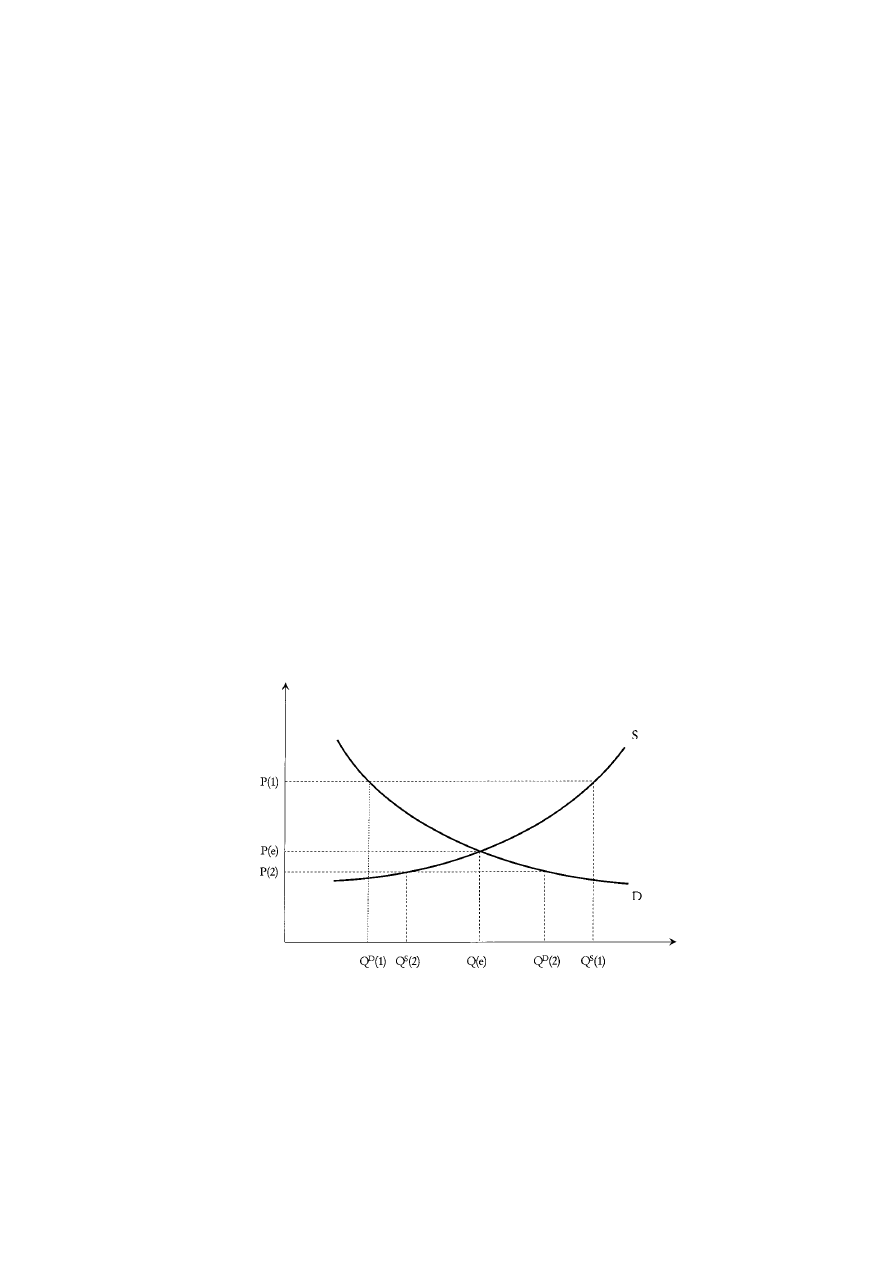
that the demand of every individual demander in every market
decreases as market price rises, or that the amount every seller offers
to supply in every market increases as market price rises. In other
words, economists recognize that individuals may well “disobey” the
“laws” of supply and demand. Moreover, there may be whole
markets that disobey these laws at particular times, so that market
supply fails to rise, or market demand fails to fall when market price
rises. Markets for stocks and markets for currencies, for example,
display annoying propensities to violate the “law of supply” and
“law of demand.” A rise in the price of Amazon.com stock can
unleash a rush of new buyers who demand more of the stock antic-
ipating further increases in price, and can shrink the supply of sellers
who become even more reluctant to part with Amazon.com while
its price is increasing. The “laws” of supply and demand certainly do
little to help us understand stock market “bubbles.” In 1997 a drop
in the price of Thailand’s currency, the bhat, triggered the Asian
financial crisis when buyers disappeared from the market afraid to
buy bhat while its price was falling, and sellers flooded the market
hoping to unload their bhat before it fell even farther in value.
Clearly the “laws” of supply and demand are not going to help us
understand the logic behind currency crises. We will take up these

Markets

Figure 4.1

Supply and Demand

“annoying” anomalies when market participants interpret changes
in market prices as signals about what direction a price is moving in
when we examine disequilibrating forces than can operate in
markets later in this chapter. But for now it is sufficient to note that
the “laws” of supply and demand should be interpreted simply as
plausible hypotheses about the behavior of buyers and sellers in
many markets under many conditions.

At this point economists invariably use a simple graph to illustrate

the laws of supply and demand. We plot market price on a vertical
axis and the quantity, or number of units all potential suppliers, in
sum total, would be willing to supply in a specified time period on
the horizontal axis. According to the law of supply as we go up the
vertical axis, at ever higher prices, the number of units all potential
suppliers would be willing to supply in a given time period, or the
“market supply,” increases. This gives us an upward sloping market
supply curve, or in different words a market supply curve with a
positive slope. Similarly, we plot market price on a vertical axis and
the quantity, or number of units all potential demanders, in sum
total, would be willing to buy in a given time period on the
horizontal axis. According to the law of demand as we go up the
vertical axis, at ever higher prices, the number of units all potential
demanders would be willing to buy, or the “market demand,”
decreases. This gives us a downward sloping market demand curve,
or in different words, a market demand curve with a negative slope.
While these are logically two separate graphs illustrating two
different “laws” or functional relationships, since the vertical axis is
the same in both cases, and the horizontal axis is measured in units
of the same good supplied or demanded in the same time period, we
can combine the two graphs into one with an upward sloping
market supply curve and a downward sloping market demand curve.
In this most familiar of all graphs in economics one must remember:
(1) the independent variable is price, and this is measured (uncon-
ventionally) on the vertical axis, while the dependent variable,
quantity supplied or demanded by market participants, is measured
(unconventionally) on the horizontal axis. (2) When using the
market supply curve the horizontal axis measures the number of
units of the good all potential suppliers would be willing to sell at
different prices. (3) When using the market demand curve the
horizontal axis measures the number of units of the good all
potential demanders would be willing to buy at different prices. (4)
There is an implicit time period buried in the units of measurement

The ABCs of Political Economy

on the horizontal axis. For example, the supply and demand curves
and the graph will look different if the horizontal axis is measured
in bushels of apples supplied and demanded per week than if it is
measured in bushels of apples supplied and demanded per month.

The “law” of uniform price

The law of uniform price says that all units of a good in a market will
sell at the same price no matter who are the buyers and sellers. This might
seem surprising since some of the deals struck will be between high
cost producers and buyers who are very desirous of the good, and
some of the deals will be struck between low cost producers and
buyers who are lukewarm about buying at all. Nonetheless, the law
of uniform price says a good will tend to sell at the same price no
matter who the seller and buyer may be. The logic of this law can be
illustrated by asking what would happen if some buyers and sellers
were arranging deals at a lower price than others for the same good.
In this case it would pay for anyone to enter the part of the market
where the good was selling at the lower price as a buyer and buy up
all they could, and then enter the part of the market where deals
were being struck at the higher price as a seller to re-sell at a profit.
This activity is called “arbitrage,” and in a free market where any
who wish can participate as buyers or sellers the activity of arbitrage
should drive all deals to be struck at the same price. Where prices
are lower arbitrage increases demand and raises price, and where
prices are higher arbitrage increases supply and lowers price – driving
divergent prices for the same good in a market closer together. Of
course, this assumes that “a rose is a rose is a rose is a rose” in the
words of one of the great French literati, Gertrude Stein – that is, that
there are no qualitative differences between different units of the
good. But subject to this assumption, and the energy levels of those
who would profit from doing nothing other than buying “cheap”
and selling “dear,” economists expect all units of a good that is
bought and sold in a “well ordered” market to sell more or less at
the same price.

The micro “law” of supply and demand

I call the third “law” the micro law of supply and demand to dis-
tinguish it from a different law we study in chapter 6 that I call the
“macro law of supply and demand.” The micro law of supply and
demand states that in a free market the uniform market price will adjust
until the number of units buyers want to buy is equal to the number of

Markets

units sellers want to sell. In terms of the supply and demand graph in
Figure 4.1, the micro law of supply and demand says that the market
will settle at the price across from where the market supply and
demand curves cross, and at the quantity bought and sold beneath
where the supply and demand curves cross. This price and this
quantity bought and sold are called the equilibrium price and equilib-
rium quantity, so another way of stating the micro law of supply and
demand is: markets will settle at their equilibrium prices, and if left to
the free market the quantity of any good that will be produced and
consumed will be the equilibrium quantity.

The rationale for the micro law of supply and demand is as

follows: Suppose the going market price, P(1), is higher than the
equilibrium price, P(e). In this case if we read across from this price
to find out how much buyers are willing to buy, Q

(1), as compared

to how much suppliers are willing to sell, Q

(1), we discover from

the market demand curve and market supply curve that buyers are
not willing to buy all that sellers are willing to sell at this price,
Q

(1) < Q

(1). In other words, at this price there will be excess supply

in the market for the good. What can we expect sellers to do? In
conditions of excess supply sellers fall into two groups: those who are
happily succeeding in selling their goods at P(1) and those who
cannot sell all they want and are therefore frustrated. Those who are
not able to sell their goods have an incentive to lower their asking
price below the going market price in order to move from the group
of frustrated sellers to the group of successful sellers, thereby driving
the market price down in the direction of the equilibrium price.
Buyers also have an incentive to only agree to buy at a price below
the going market price when they notice there is excess supply in
the market since they know that there are some frustrated sellers out
there who should be willing to accept less than the going market
price, providing another reason why market price should start to fall
in the direction of the equilibrium price.

On the other hand, suppose the going market price, P(2), is lower

than the equilibrium price, P(e). If we read across from this price to
find out how much buyers are willing to buy, Q

(2), as compared to

how much suppliers are willing to sell, Q

(2), we discover from the

market demand curve and market supply curve that sellers are not
willing to sell all that buyers are willing to buy at this price, Q

(2) <

(2). In other words, at this price there will be excess demand in

the market for the good. What can we expect buyers to do? In
conditions of excess demand buyers fall into two groups: those who

The ABCs of Political Economy

are happily able to buy all the good they want at P(2), and those who
are not able to buy all they want and are therefore frustrated. Those
who are not able to buy all they want have an incentive to raise their
offer price above the going market price in order to move from the
group of frustrated buyers to the group of successful buyers, thereby
driving the market price up in the direction of the equilibrium price.
Sellers also have an incentive to only agree to sell at a price above the
going market price when they notice there is excess demand in the
market since they know that there are some frustrated buyers who
should be willing to pay more than the going market price,
providing another reason why market price should rise in the
direction of the equilibrium price.

So for actual market prices above the equilibrium price there are

incentives for frustrated sellers to cut their asking price and buyers
to offer a lower price, driving the market price down toward the equi-
librium price. And as the market price drops the amount of the
excess supply will decrease since the law of supply says that supply
decreases as price falls and the law of demand says that demand
increases as price falls. And for market prices below the equilibrium
price there are incentives for frustrated buyers to raise their offer
price and for sellers to raise their asking price, driving the market
price up toward the equilibrium price. And as the market price rises
the excess demand will decrease since the law of demand says that
demand decreases as price rises, and the law of supply says that
supply increases as price rises. So according to the micro law of
supply and demand, the only stable price will be the equilibrium
price because self-interested behavior of frustrated sellers or buyers
will lead to changes in price under conditions of both excess supply
and excess demand, and only at the equilibrium price is there
neither excess supply nor excess demand. This particular kind of self-
interested behavior of buyers and sellers – individually rational
responses to finding oneself unable to sell or buy all one wants at
the going market price – can be thought of as “equilibrating forces”
that economists expect to operate in markets. So the micro law of
supply and demand can be thought of as a “law” explaining why
there should be equilibrating forces at work in markets. We will
discover below that market enthusiasts and critics disagree about
how strong these “equilibrating forces” are compared to “disequili-
brating forces” the micro law of supply and demand does not alert
us to that sometimes operate alongside equilibrating forces.

Markets

There are a few things worth noting at this point:

1. There are different senses in which buyers or sellers are

“satisfied.” All buyers would always like to pay a lower price, and
all sellers would always like to receive a higher price. So in that
sense, neither buyers nor sellers are ever “satisfied” no matter
what the going price. But when the market price is above the
equilibrium price, while successful sellers will be pleased, there
will be unsuccessful sellers who will be displeased. Moreover,
there is something the non-sellers can do about their frustrations:
they can offer to sell at a lower price. Similarly, when the market
price is below the equilibrium price, while successful buyers will
be pleased, there will be unsuccessful buyers who will be
displeased. And what the non-buyers can do about their frustra-
tions is to offer to pay a higher price.

2. It is always the case that the quantity bought will be equal to the

quantity sold – whether the market is in equilibrium or not. This
follows because every unit that was bought was sold and every
unit that was sold was bought! But that is not the same as saying
that the quantity demanders want to buy is equal to the quantity
suppliers want to sell. There is only one price at which the
quantity demanded will equal the quantity supplied – the equi-
librium price. At all other prices there will be either excess supply
or excess demand.

3. Since not all markets are always in equilibrium, how much will

be bought and sold when a market is out of equilibrium? This is
where the assumption of non-coercion in our definition of a
market enters in: buyers cannot be forced to buy if they don’t
want to and sellers can’t be forced to sell if they don’t want to.
When there is excess supply the sellers would like to sell more
than the buyers want to buy at the going price. So under
conditions of excess supply it is the buyers who have the upper
hand, in a sense, and they will determine how much is going to
be bought, and therefore sold. In Figure 4.1 when market price is
P(1) and there is excess supply buyers will only buy Q

(1) and

therefore, that is all sellers, will be able to sell. When there is
excess demand the buyers would like to buy more than the sellers
want to sell. So under conditions of excess demand it is the sellers
who have the upper hand and will determine how much is going
to be sold, and therefore bought. In Figure 4.1 when market price
is P(2) and there is excess demand sellers will only sell Q

(2) and

therefore, that is all buyers will be able to buy.

The ABCs of Political Economy

Elasticity of supply and demand

The law of demand just says that as price rises we expect the quantity
demanded to fall. It doesn’t say whether demand will fall a lot or a
little. If a 1% increase in price leads to more than a 1% fall in quantity
demanded, we say that market demand is elastic. If a 1% increase in price
leads to less than a 1% fall in quantity demanded, we say that market
demand is inelastic. Similarly, the law of supply just says that as price
rises we expect the quantity supplied to rise; it doesn’t say whether
supply will rise a lot or a little. If a 1% increase in price leads to more
than a 1% rise in quantity supplied, we say that market supply is
elastic. If a 1% increase in price leads to less than a 1% rise in
quantity supplied, we say that market supply is inelastic.

The elasticity of supply and demand allows us to predict how

much the supply and demand for goods will change when their price
changes. Elasticity also holds the key to how revenues of sellers will
be affected by changes in supply. For example, the demand for corn
is usually elastic. So when a drought hits the corn belt the price will
rise and the equilibrium quantity bought and sold will fall. But the
percentage fall in sales will be greater than the percentage increase
in price because demand for corn is elastic. Since the revenue of corn
farmers is simply equal to the market price times the quantity sold,
the fact that sales drop by a greater percent than the increase in price
means revenues must fall. On the other hand, the demand for oil is
usually inelastic. So if war breaks out in the Middle East and a
country such as Iraq, Kuwait, Iran, Libya, or Saudi Arabia is tem-
porarily eliminated as a potential supplier the price will rise and the
equilibrium quantity bought and sold will fall as before. But because
demand for oil is inelastic the percentage fall in sales will be less than
the percentage increase in price. In this case the revenue of oil
suppliers will increase because the rise in price outweighs the drop
in sales when supply decreases.

You can use your understanding of elasticity to predict whether

more or less unemployment will result from minimum wage laws,
and whether more or fewer shortages will result from price controls.
Draw a labor market diagram with one “flat” (elastic) labor demand
curve and one “steep” (inelastic) labor demand curve where both
demand curves cross the labor supply curve at the same point.
Where both demand curves cross the supply curve determines the
equilibrium wage rate and the equilibrium level of employment.
Now draw in a minimum wage above the equilibrium wage and see

Markets

what happens to employment as buyers (employers) determine the
quantity that will be bought and sold in a market with excess supply.
Notice that the drop in employment is greater if the demand for
labor is more elastic, and smaller if the demand for labor is more
inelastic. Draw a diagram for the steel market with one “flat” or
elastic supply curve and one “steep” or inelastic supply curve where
both supply curves cross the demand curve for steel at the same
point. Where both supply curves cross the demand curve determines
the equilibrium price of steel and the equilibrium quantity of steel
production. Now draw a price ceiling below the equilibrium price
and see what happens to production when suppliers determine the
amount that will be sold and bought in a market with excess
demand. Notice that the drop in production and shortage is greater
if the supply of steel is more elastic and smaller if the supply of steel
is more inelastic.

The principal factors that determine the elasticity of market

demand are the availability and closeness of substitutes for the good,
and the organization and bargaining power of potential buyers. The
principal factors that determine the elasticity of market supply are
the mobility of productive factors into and out of the industry and
the organization and bargaining power of potential sellers.

THE DREAM OF A BENEFICENT INVISIBLE HAND

Adam Smith noticed something strange but wonderful about free
markets. He saw competitive markets as a kind of beneficent,
“invisible hand” that guided “the private interests and passions of
men” in the direction “which is most agreeable to the interest of the
whole society.” Smith expressed this view, in perhaps the most
widely quoted passage in all of economics in The Wealth of Nations
published in 1776:

Every individual necessarily labours to render the annual revenue
of the society as great as he can. He generally, indeed, neither
intends to promote the public interest, nor knows how much he
is promoting it. He intends only his own gain, and he is in this,
as in many other cases, led by an invisible hand to promote an end
which was no part of his intention. Nor is it always the worse for
the society that it was no part of it. By pursuing his own interest
he frequently promotes that of the society more effectually than

The ABCs of Political Economy

when he really intends to promote it ... It is not from the benev-
olence of the butcher, the brewer, or the baker that we expect our
dinner, but from their regard to their self-interest. We address
ourselves, not to their humanity, but to their self-love, and never
talk to them of our necessities, but of their advantages.

In the words of Robert Heilbroner: “Adam Smith’s laws of the market
are basically simple. They show us how the drive of individual self-
interest in an environment of similarly motivated individuals will
result in competition; andthey further demonstrate how competi-
tion will result in the provision of those goods that society wants,
in the quantities that society desires.”

But how does this miracle

happen?

Suppose consumers’ taste for apples increases and their taste for

oranges decreases – for whatever reason. Assuming consumers know
best what they like, how would we want the economy to respond to
this new situation? If there were an omniscient, beneficent God in
charge of the economy she would shift some of our scarce productive
resources – land, labor, fertilizer, etc. – out of orange production and
into apple production. What would a system of free markets do?
These changes in consumer tastes would shift the market demand
curve for apples out to the right indicating that consumers now
would demand more apples at each and every price of apples than
before, and the market demand curve for oranges back to the left
indicating that consumers would now demand fewer oranges at each
and every price than before – leading to excess demand for apples
and excess supply of oranges at their old equilibrium prices. The
micro law of supply and demand would drive the price of apples up
until the excess demand for apples was eliminated and the price of
oranges down until the excess supply of oranges was eliminated. At
the new higher price of apples, the law of supply tells us that former
apple growers, and any new ones drawn into the industry by the
higher price of apples, would increase production of apples by
purchasing more land, labor, fertilizer, etc. At the new lower price of
oranges the law of supply tells us that orange growers would decrease
their production of oranges by using less land, labor, and fertilizer,
etc. to grow oranges. Bingo! As if guided by an invisible hand,
without anyone thinking or planning at all, the free market does
what a beneficent God would have done for us!

Markets

1. Robert Heilbroner, The Worldly Philosophers (Simon and Schuster, 1992): 55.

Or, suppose agronomists develop a new strain of apple that can

be grown with less land between trees than before. This is a technical
change that reduces the amount of scarce productive resources it
takes to grow apples compared to the past. An omniscient,
beneficent God would have consumers buy more apples and fewer
oranges now that apples are less socially costly. What will free
markets do? The cost-reducing change in apple growing technology
will shift the market supply curve for apples out to the right because
now apple growers can cover the cost of growing more apples than
before at each and every price – producing an excess supply of apples
at the old equilibrium price. The micro law of supply and demand
will lower apple prices until the excess supply is eliminated and we
reach the new equilibrium in the apple market. And the law of
demand tells us that consumers will buy more apples at the lower
price. Meanwhile, over in the orange market, the fall in the price of
apples leads some fruit buyers to substitute apples for oranges which
shifts the demand curve for oranges back to the left indicating that
fewer oranges will be demanded at each and every price of oranges
now that the price of apples is lower – creating excess supply in the
orange market. This will lead to a fall in the price of oranges and
lower levels of orange production. Bingo! The free market will bring
about an increase in apple production and consumption and a
decrease in orange production and consumption when the social
cost of producing apples decreases relative to the social cost of
producing oranges – just what we would have wanted to happen.

We can combine Figure 2.2: The Efficiency Criterion (p. 33) and

Figure 4.1: Supply and Demand (p. 73) to see what Smith’s
conclusion that markets harness individually rational behavior to
yield socially rational outcomes amounts to. According to the micro
law of supply and demand, the market outcome will be the equilib-
rium outcome, and the number of apples produced and consumed
can be found directly below where the market supply curve crosses
the market demand curve. According to the efficiency criterion the
optimal number of apples to produce and consume can be found
directly below where the marginal social cost curve crosses the
marginal social benefit curve. So the market outcome will yield the
socially efficient outcome if and only if the market supply curve
coincides with the MSC curve and the market demand curve
coincides with the MSB curve. Another way to put it is that if and
only if market supply closely approximates marginal social cost and

The ABCs of Political Economy

market demand closely approximates marginal social benefits will
free market outcomes be socially efficient outcomes.

But do market supply and demand reasonably express marginal

social costs andbenefits? That is one way to see the debate between
those who see market allocations as being guided by an invisible
handversus those who see them as being misguidedby an invisible
foot. If market supply anddemandclosely approximate true marginal
social costs and benefits then the individually rational behavior of
buyers andsellers andthe workings of the micro law of supply and
demandwouldbe working in the social interest because they would
be driving production and consumption of goods and services toward
socially efficient levels. Moreover, whenever conditions changed
social costs or benefits these equilibrating forces wouldmove us to
the new socially efficient outcome. In other words, markets would
yieldefficient allocations of scarce productive resources. On the other
hand, if there are significant discrepancies between market supply
andmarginal social costs and/or market demandandmarginal social
benefits, individually rational behavior of buyers and sellers and the
micro law of supply anddemandwork against the social interest by
driving us to produce too little of some goods and too much of
others. In other words, by relying on market forces we would con-
sistently get inefficient allocations of productive resources.

Mainstream and political economists agree on one part of the

answer before parting company. They agree that what market supply
captures and represents are the costs born by the actual sellers of goods
and services; and what market demand represents are the benefits enjoyed
by the actual buyers of goods and services. We call these “private costs”
and“private benefits.” A rational buyer will keep buying a good as
long as the private benefit to her of an additional unit is at least as
great as the price she must pay for it. In other words, her marginal
private benefit curve is her individual demand curve. Since the
market demand curve is simply the summation of all individual
demand curves, the market demand curve is simply the sum of all
marginal private benefit curves. A rational seller will keep selling as
long as the cost to her of producing another unit of output is no
greater than the price she will get from selling it. In other words, her
marginal private cost curve is her individual supply curve. Since
market supply is simply the summation of all individual supply
curves, the market supply curve is simply the sum of all marginal
private cost curves. So the question becomes: When do private costs
and benefits differ from social costs and benefits?

Markets

In fairness to Adam Smith, the distinction between private and

social costs andbenefits was not clear in his lifetime. Smith, and
“classical economists” who livedandwrote after him as well,
conflatedsocial andprivate costs andbenefits andnever askedif
anyone other than the seller bore part of the cost of increased
production, or anyone other than the buyer enjoyed part of the
benefit of increased consumption of different kinds of goods and
services. The modern terminology for differences between social and
private costs of production is “a production externality.” And the
name for the difference between social and private benefits from con-
sumption is “a consumption externality.” These “external effects”
can be negative if someone other than the seller suffers a cost
associatedwith production so social costs exceedprivate costs, or if
someone other than the buyer is adversely affected by the buyer’s
consumption so private benefits exceedsocial benefits. Or external
effects can be positive if the private costs of production exceed the
social costs or social benefits of consumption exceedprivate benefits.
Adam Smith’s vision of the market as a mechanism that successfully
harnesses individual desires to the social purpose of using scarce
productive resources efficiently hinges on the assumption that
external effects are insignificant. And, indeed, this is precisely the
un-emphasizedassumption that lies behindthe mainstream
conclusion that markets are remarkable efficiency machines that
require little social effort on our part. In fact, the mainstream view
today is a strident echo of Adam Smith’s conclusion that the only
“effort” requiredis the “effort” to resist the temptation to tamper
with the free market place andsimply: “laissez faire.”

THE NIGHTMARE OF A MALEVOLENT INVISIBLE FOOT

Mainstream economic theory teaches that the problem with exter-
nalities is that the buyer or seller has no incentive to take the
external cost or benefit for others into account when deciding how
much of something to supply or demand. And Mainstream theory
teaches that the “problem” with public goods is that nobody can be
excluded from benefitting from a public good once anyone buys it,
and therefore everyone has an incentive to “ride for free” on the
purchases of others rather than revealing their true willingness to
pay for public goods by purchasing them in the market place. In
other words, mainstream economics concedes that the laws of the
market place will lead to inefficient allocations of scarce productive

The ABCs of Political Economy

resources when public goods and externalities come into play
because important benefits or costs go unaccounted for in the
market decision making process. If anyone cares to listen, standard
economic theory predicts that market forces will lead us to produce
too much of goods whose production and/or consumption entail
negative externalities, too little of goods whose production and/or
consumption entail positive externalities, and much too little, if any,
public goods. We can see the problem of negative externalities by
looking at the automobile industry, and the problem of public goods
by considering pollution reduction.

Externalities: the auto industry

The micro law of supply and demand tells us how many cars will be
produced and consumed if we leave the decision to the free market.
The price of cars will adjust until there is neither excess supply nor
excess demand at which point the “equilibrium” number of cars will
be produced and consumed. The question is whether or not this is
more, less, or the same number of cars that is socially efficient, or
optimal to produce and consume. As we saw, the socially efficient
level of auto production and consumption is where the MSB curve
crosses the MSC curve. If the market supply curve for cars coincides
with the MSC curve for cars, and if the market demand curve for cars
coincides with the MSB curve for cars, the market outcome will be
the efficient outcome. Otherwise, it will not.

Let us assume that the market supply curve for cars does a

reasonably good job of approximating the marginal private costs the
makers and sellers of cars incur. That is, we will assume that if car
manufacturers can get a price for a car that is something above what
it costs them to make it, they will produce and sell the car. In this
case the market supply curve, S, closely approximates the marginal
private cost (MPC) curve for making cars: S = MPC. But if there are
costs to external parties above and beyond the costs of inputs car
makers must pay for, there is no reason to expect the car makers to
take them into account. So if the corporations making cars in Detroit
also pollute the air in ways that cause acid rain, the costs that take
the form of lost benefits to those who own, use, or enjoy forests and
lakes in Eastern Canada and the United States will not be taken into
account by those who make the decisions about how many cars to
produce. Nevertheless, along with the cost of steel, rubber and labor
needed to make a car – which are costs borne by car manufacturers
– the costs of acid rain are part of the social costs of making cars even

Markets

if they are not borne by car makers. To the cost of steel, rubber, and
labor that comprise the private costs of making a car, must be added
the damage from acid rain that occurs when we make a car if we are
to have the full cost to society of making another car. In other words,
the marginal social cost of making a car, MSC, is equal to the
marginal private cost of making the car, MPC, plus the marginal
external costs associated with making the car, MEC: MSC = MPC +
MEC. Since MEC is positive for automobile production, marginal
social cost always exceeds marginal private cost, which means the
marginal social cost curve for producing cars lies somewhere above
the marginal private cost curve for making cars, which is, in turn,
roughly equal to the market supply curve for cars: MSC = MPC +
MEC = S + MEC with MEC > 0.

When car buyers consider whether or not to purchase a car they

presumably compare the benefit they expect to get in the form of
ease and speed of transportation with the price they will have to pay
out of their limited income. If the private benefit exceeds the price,
they will buy the car, and if it does not, they won’t. This means the
market demand curve, D, represents the marginal private benefit
curve from car consumption, MPB, reasonably well: D = MPB. But I
am not the only person affected when I “consume” my car. When I
drive my car the exhausts add to the “greenhouse” gases in the
atmosphere and contribute to global warming. When I drive from
the suburbs through inner city neighborhoods I contribute to urban
smog, noise pollution, and congestion. In other words, when I
consume a car there are others who suffer negative benefits which
means that the social benefit of consuming another car is less than
the private benefit of consuming another car. So even if the market
demand curve for cars reasonably represents the marginal private
benefits of car consumption, it overestimates the marginal social
benefits of car consumption because it ignores the negative impact
of car consumption on those not driving them. The marginal social
benefits from consuming another car, MSB, is equal to the marginal
private benefits to the car buyer plus the marginal external benefits
to others, MEB: MSB = MPB + MEB. But in the case of car consump-
tion the marginal external “benefits,” MEB, are negative. This implies
that the marginal social benefit curve lies somewhere below the
market demand curve for automobiles: MSB = MPB + MEB = D + MEB
with MEB < 0.

The ABCs of Political Economy

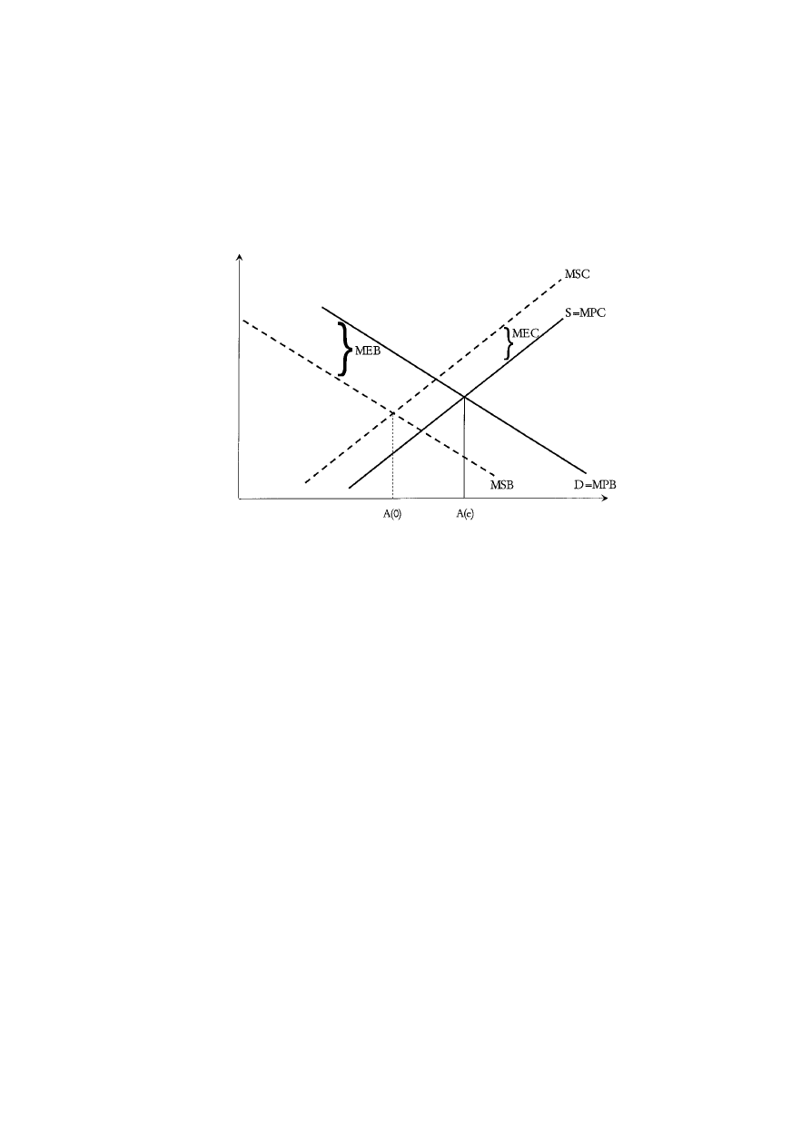
But as can be seen in Figure 4.2, if the MSC curve lies above the

market supply curve, and the MSB curve lies below the market
demand curve for cars, MSC and MSB will cross to the left of where
the market supply and demand curves cross. Therefore the socially
efficient, or optimal level of automobile production (and consump-
tion), A(0), will be less than the equilibrium level of production and
consumption, A(e), that the micro law of supply and demand will
drive us toward. In other words, the market will lead us to produce
and consume more cars than is socially efficient, or optimal. The
market will lead to too much car production and consumption
because sellers and buyers decide how many cars to produce and
consume and they have no reason to take anything other than the
costs and benefits to them into account. They have no incentive to
consider the external costs associated with producing and
consuming cars. In fact, they have good reason to ignore these
external effects because taking them into account would make them
individually worse off. Not surprisingly we discover that if decision
makers ignore negative consequences of doing something – in this
case the negative external effects of car production and consump-
tion on people other than the car producer and buyer – they will

Markets

Figure 4.2

Inefficiencies in the Automobile Market

decide to do too much of it – in this case they will decide to produce
and consume too many cars.

Public goods: pollution reduction

A public good is a good produced by human economic activity that
is consumed, to all intents and purposes, by everyone rather than
by an individual consumer. Unlike a private good such as underwear
that affects only its wearer, public goods like pollution reduction
affect most people. In different terms, nobody can be excluded from
“consuming” a public good – or benefitting from the existence of
the public good. This is not to say that everyone has the same pref-
erences regarding public goods anymore than people have the same
preferences for private goods. I happen to prefer apples to oranges,
and I value pollution reduction more than I value so-called “national
defense.” There are others who place greater value on “national
defense” than they do on pollution reduction, just as there are others
who prefer oranges to apples. But unlike the case of apples and
oranges where those who prefer apples can buy more apples and
those who like oranges more can buy more oranges, all US citizens
have to “consume” the same amount of federal spending on the
military and federal spending on pollution reduction. We cannot
provide more military spending for the US citizens who value that
public good more, and more pollution reduction for the US citizens
who value the environment more. Whereas different Americans can
consume different amounts of private goods, we all must live in the
same “public good world.”

What wouldhappen if we left the decision about how much of

our scarce productive resources to devote to producing public goods
to the free market? Markets only provide goods for which there is
what we call “effective demand,” that is, buyers willing and able to
put their money where their mouth is. But what incentive is there for
a buyer to pay for a public good? First of all, no matter how much I

The ABCs of Political Economy

2. External effects are notoriously hard to measure in market economies.

This is of great significance since their magnitude is critical to how inef-
ficient a market will be, and how large a pollution tax needs to be to correct
the inefficiency. In a 1998 report the Center for Technology Assessment
estimated that when external effects are taken into account the true social
cost of a gallon of gasoline consumed in the US may be as high as $15. I
just paid $1.02 a gallon when I filled my car up today in southern Maryland.
The $1.02 already includes some hefty taxes, but obviously they are not
nearly hefty enough!

value the public good, I only enjoy a tiny fraction of the overall, or
social benefit that comes from having more of it since I cannot
exclude others who do not pay for it from benefitting as well. In
different terms: Social rationality demands that an individual
purchase a public goodup to the point where the cost of the last unit
she purchasedis as great as the benefits enjoyedby all who benefit,
in sum total, from her purchase of the good. But it is only rational for
an individual to buy a public good up to the point where the cost of
the last unit she purchasedis as great as the benefit she, herself,
enjoys from the good. When individuals buy public goods in a free
market they have no incentive to take the benefits others enjoy into
account when they decide how much to buy. Consequently they
“demand” far less than is socially efficient, if they purchase any at all.
In sum, market demand will grossly under-represent the marginal
social benefit of public goods.

Another way to see the problem is to recognize that each potential

buyer of a public good has an incentive to wait and hope that
someone else will buy the public good. A patient buyer can “ride for
free” on others’ purchases since non-payers cannot be excluded from
benefitting from public goods. But if everyone is waiting for
someone else to plunk down their hard earned income for a public
good, nobody will demonstrate “effective demand” for public goods
in the market place. “Free riding” is individually rational in the case
of public goods – but leads to an “effective demand” for public goods
that grossly underestimates their true social benefit. In chapter 5 we
explore this logic formally in “the public good game.”

What prevents a group of people who will benefit from a public

good from banding together to express their demand for the good
collectively? The problem is that there is an incentive for people to
lie about how much they benefit. If the associations of public good
consumers are voluntary, no matter how much I truly benefit from
a public good, I am better off pretending I don’t benefit at all. Then
I can decline membership in the association and avoid paying
anything, knowing full well that I will, in fact, benefit from its
existence nonetheless. If the associations are not voluntary – i.e., if
a government “drafts” people into the public good consuming
coalition – there is still an incentive for people to under-represent
the degree to which they benefit if assessments are based on degree
of benefit. This is where the fact that not all people do benefit equally
from different kinds of public goods becomes an important part of
the problem. If we knew that everyone truly valued a larger military

Markets

to the same extent, there would be few objections to making
everyone contribute the same amount to pay for it. But there is every
reason to believe this is not the case. In this context, if we believe
that payments should be related to the degree to which someone
benefits, there is an incentive for everyone to pretend they benefit
less than they do. If the effective demand expressed by the non-
voluntary consuming coalition is based on these individually
rational under-representations, it will still significantly under-
represent the true social benefits people enjoy from the public good,
and consequently lead to less demand for the public good than is
socially efficient, or optimal.

In sum, because of what economists call the “free rider” incentive

problem andthe “transaction costs” of organizing andmanaging a
coalition of public goodconsumers, market demandpredictably
under-represents the true social benefits that come from consump-
tion of public goods. If the production of a public good entails no
external effects so the market supply curve accurately represents the
marginal social costs of producing the public good, then since market
demand will lie considerably under the true marginal social benefit
curve for the public good, the market equilibrium level of production
andconsumption will be significantly less than the socially efficient
level. In conclusion, if we left it to the free market andvoluntary
associations precious little, if any, of our scarce productive resources
wouldbe usedto produce public goods no matter how valuable they
really were. As Robert Heilbroner put it: “The market has a keen ear
for private wants, but a deaf ear for public needs.”

The fact that pollution reduction is a public good has important

implications for green consumerism in free market economies. There
are a number of cheap detergents that get my wash very white but
cause considerable water pollution. “Green” detergents, on the other
hand, are more expensive and leave my whites more gray than
white, but cause less water pollution. Whether or not I end up making
the socially responsible choice, because pollution reduction is a public
good the market provides too little incentive for me to make the
socially efficient choice. My own best interests are served by
weighing the disadvantage of the extra cost and grayer whites to me
against the advantage to me of the diminution in water pollution
that would result if I use the green detergent. But presumably there
are many others besides me who also benefit from the cleaner water
if I buy the green detergent – which is precisely why we think of
“buying green” as socially responsible behavior. Unfortunately the

The ABCs of Political Economy

market provides no incentive for me to take their benefit into
account. Worse still, if I suspect others may consult only their own
interests when they choose which detergent to buy, i.e., if I think
they will ignore the benefits to me and others if they choose the
“green” detergent, by choosing to take their interests into account
and consuming green myself I risk not only making a choice that
was detrimental to my own interests, I risk being played for a sucker
as well.

This is not to say that many people will not choose to “do the

right thing” and “consume green” in any case. Moreover, there may
be incentives other than the socially counterproductive market incentives
that may overcome the market disincentive to consume green. The
fact that I am a member of the Southern Maryland Green Party and
fear I would be ostracized if observed by a fellow party member with
a polluting detergent in my shopping basket in the check out line at
the supermarket is apparently a powerful enough incentive in my
own case to lead me to buy a green detergent despite the market dis-
incentive to do so. (Admittedly I have only a slight preference for
white over gray clothes, and who knows how long I will hold out if
the price differential increases?) But the point is that because
pollution reduction is a public good, market incentives are perverse,
i.e. lead people to consume less “green” and more “dirty” than is
socially efficient. The extent to which people ignore the perverse
market incentives and act on the basis of concern for the environ-
ment, concern for others, including future generations, or in
response to non-market, social incentives such as fear of ostracism
is important for the environment and the social interest, but does
not make the market incentives any the less perverse.

The prevalence of external effects

In face of these concessions – markets misallocate resources when
there are externalities and public goods – how do market enthusi-
asts continue to claim that markets allocate resources efficiently – as
if guided by a beneficent invisible hand? The answer lies in an
assumption that is explicit in the theorems of graduate level micro

Markets

3. Most detergents call for a full cup per load of wash. Church & Dwight

canceled a

⁄

cup laundry detergent product when consumer demand for

this “green” product proved insufficient. See Christine Canning, “The
Laundry Detergent Market,” in Household and Personal Products Industry,
April 1996.

economic theory texts but only implicit in undergraduate textbooks
and in the advice of most economists. The fundamental theorem of
welfare economics states that if all markets are in equilibrium the
economy will be in a Pareto optimal state only if there are no external
effects or public goods. The assumption that there are no public goods
or external effects is explicit in the statement of the theorem that is
the modern incarnation of Adam Smith’s 200-year-old vision of an
invisible hand – because otherwise the theorem would be false! Since
everyone knows there are externalities and public goods in the real
world, the conclusion that markets allocate resources reasonably effi-
ciently in the real world rests on the assumption that external effects
and public goods are few and far between. This assumption is usually
unstated, and its validity has never been demonstrated through
empirical research. It is a presumption implicit in an untested
paradigm that lies behind mainstream economic theory – a
paradigm that pretends that the choices people make have little
effect on the opportunities and well being of others.

If we replace the implicit paradigm at the basis of mainstream

economics with one that sees the world as a web of human interac-
tion where people’s choices often have far reaching consequences
for others, both now and in the future, the presumption that
external effects and public goods are the exception rather than the
rule is reversed. Since political economists have long seen the world
in just this way, and everything we have learned about the relation
between human choices and ecological systems over the past 30
years reinforces this vision of interconnectedness, there is every
reason for political economists to expect external and public effects
to be the rule rather than the exception. What is surprising is that so
few political economists have recognized the far reaching implica-
tions of their own beliefs when it comes to assessing the efficiency
of markets. One stellar exception is E.K. Hunt. In an article “On
Lemmings and Other Acquisitive Animals” remarkable for its lack of
impact on other political economists when published in June 1973
(Journal of Economic Issues), E.K. Hunt stated the “reverse”
assumption as follows:

The Achilles heel of welfare economics [as practiced by
mainstream pro-market economists] is its treatment of externali-
ties ... When reference is made to externalities, one usually takes
as a typical example an upwind factory that emits large quantities
of sulfur oxides and particulate matter inducing rising probabili-
ties of emphysema, lung cancer, and other respiratory diseases to

The ABCs of Political Economy

residents downwind, or a strip-mining operation that leaves an
irreparable aesthetic scar on the countryside. The fact is, however,
that most of the millions of acts of production and consumption
in which we daily engage involve externalities. In a market
economy any action of one individual or enterprise which induces
pleasure or pain to any other individual or enterprise ... consti-
tutes an externality. Since the vast majority of productive and
consumptive acts are social, i.e., to some degree they involve more
than one person, it follows that they will involve externalities.
Our table manners in a restaurant, the general appearance of our
house, our yard or our person, our personal hygiene, the route we
pick for a joy ride, the time of day we mow our lawn, or nearly
any one of the thousands of ordinary daily acts, all affect, to some
degree, the pleasures or happiness of others. The fact is ... exter-
nalities are totally pervasive ... Only the most extreme bourgeois
individualism could have resulted in an economic theory that
assumed otherwise.

If the social effects of production and consumption frequently
extend beyond the sellers and buyers of those goods and services, as
Hunt argues above, and if these external effects are not insignificant,
markets will frequently misallocate resources leading us to produce
too much of some goods and too little of others. By ignoring
negative external effects markets lead us to produce and consume
more of goods like automobiles than is socially efficient. By ignoring
positive external effects markets lead us to consume less of goods
like tropical rain forests that recycle carbon dioxide and thereby
reduce global warming than is socially efficient – instead we clear
cut them or burn them off to pasture cattle. And while markets
provide reasonable opportunities for people to express their prefer-
ences for goods and services that can be enjoyed individually with
minimal “transaction costs,” they do not provide efficient means for
expressing desires for goods that are enjoyed, or consumed socially,
or collectively – like public space and pollution reduction. Markets
create “free rider” disincentives for those who would express their
desires for public goods individually, and pose daunting transaction
costs for those who attempt to form a coalition of beneficiaries. In
other words, markets have an anti-social bias.

Worse still, markets provide powerful incentives for actors to take

advantage of external effects in socially counterproductive ways, and
even to magnify or create new ones. Increasing the value of goods

Markets

and services produced, and decreasing the unpleasantness of what
we have to do to get them, are two ways that producers can increase
their profits in a market economy. And competitive pressures will
drive producers to do both. But maneuvering to appropriate a greater
share of the goods and services produced by externalizing costs and
internalizing benefits without compensation are also ways to
increase profits. Competitive pressures will drive producers to pursue
this route to greater profitability just as assiduously. Of course the
problem is, while the first kind of behavior serves the social interest
as well as the private interests of producers, the second kind of
behavior does not. Instead, when buyers or sellers promote their
private interests by externalizing costs onto those not party to the
market exchange, or internalizing benefits without compensating
external parties, their “rent seeking behavior” introduces inefficien-
cies that lead to a misallocation of productive resources and
consequently decreases the value of all the goods and services
produced. Questions market admirers seldom ask are: Where are
firms most likely to find the easiest opportunities to expand their
profits? How easy is it to increase the quantity or quality of goods
produced? How easy is it to reduce the time or discomfort it takes to
produce them? Alternatively, how easy is it to enlarge one’s slice of
the economic pie by externalizing a cost, or by appropriating a
benefit without compensation? In sum, why should we assume that
it is infinitely easier to expand profits by productive behavior than
by rent seeking behavior? Yet this implicit assumption is what lies
behind the view of markets as efficiency machines.

Market enthusiasts fail to notice that the same feature of market

exchanges primarily responsible for small transaction costs –
excluding all affected parties but two from the transaction – is also
a major source of potential gain for the buyer and seller. When the
buyer and seller of an automobile strike their convenient deal, the
size of the benefit they have to divide between them is greatly
enlarged by externalizing the costs onto others of the acid rain
produced by car production, and the costs of urban smog, noise
pollution, traffic congestion, and greenhouse gas emissions caused
by car consumption. Those who pay these costs, and thereby enlarge
car maker profits and car consumer benefits, are “easy marks” for car
sellers and buyers because they are geographically and chronologi-
cally dispersed, and because the magnitude of the effect on each of
them is small and unequal. Individually they have little incentive to

The ABCs of Political Economy

insist on being party to the transaction. Collectively they face trans-
action cost and free rider obstacles to forming a voluntary coalition
to represent a large number of people – each with little, but different,
amounts at stake.

Moreover, the opportunity for socially counterproductive rent

seeking behavior is not eliminated by making markets perfectly com-
petitive or entry costless, as is commonly assumed. Rent seeking at
the expense of a buyer or seller may be eliminated by competitive
markets, i.e. the presence of innumerable sellers for buyers to choose
from and innumerable buyers for sellers to choose from. But even if
there were countless perfectly informed sellers and buyers in every
market, even if the appearance of the slightest differences in average
profit rates in different industries induced instantaneous self-
correcting entries and exits of firms, even if every market participant
were equally powerful and therefore equally powerless – in other
words, even if we embrace the full fantasy of market enthusiasts –
as long as there are numerous external parties with small but
unequal interests in market transactions, those external parties will
face greater transaction cost and free rider obstacles to a full and
effective representation of their collective interest than any obstacles
faced by the buyer and seller in the exchange. And it is this unavoid-
able inequality that makes external parties easy prey to rent seeking
behavior on the part of buyers and sellers. Even if we could organize
a market economy so that buyers and sellers never faced a more or
less powerful opponent in a market exchange, this would not change
the fact that each of us has smaller interests at stake in many trans-
actions in which we are neither the buyer nor seller. Yet the sum total
interest of all external parties can be considerable compared to the
interests of the buyer and the seller. It is the transaction cost and free
rider problems of those with lesser interests that create an unavoid-
able inequality in power, which, in turn, gives rise to the opportunity
for individually profitable but socially counterproductive rent
seeking on the part of buyers and sellers in even the most competi-
tive markets. A sufficient condition for buyers and sellers to profit
in socially counterproductive ways from maneuvering, rent seeking,
or cost shifting behavior is that each one of us has diffuse interests
that make us affected external parties to many exchanges in which
we are neither buyer nor seller – no matter how competitive markets
may be.

Markets

But socially counterproductive rent seeking behavior is not only

engaged in at the expense of parties external to market exchanges.
The real world bears little resemblance to a game where all buyers
and sellers are equally powerful, in which case it would be pointless
for sellers or buyers to try to take advantage of one another. In the
real world it is often easier for powerful firms to increase profits by
lowering the prices they pay less powerful suppliers and raising the
prices they charge powerless consumers than it is to search for ways
to increase the quality of their products. In the real world there are
consumers with little information, time, or means to defend their
interests. There are small, capital poor, innovative firms for giants
like IBM and Microsoft to buy up instead of tackling the hard work
of innovation themselves. There are common property resources
whose productivity can be appropriated at little or no cost as they are
overexploited at the expense of future generations. And finally, there
is a government run by politicians whose careers rely principally on
their ability to raise campaign money, begging to be plied for tax
dodges and corporate welfare programs financed at taxpayer
expense. In other words, in the real world where buyers and sellers
are usually not equally powerful, the most effective profit
maximizing strategy is often to outmaneuver less powerful market
opponents and expand one’s slice of the pie at their expense rather
than work to expand it.

Snowballing inefficiency

To the extent that consumer preferences are endogenous the degree
of misallocation that results from uncorrected external effects in
market economies will increase, or “snowball” over time. As people
adjust their preferences to the biases created by external effects in
the market price system, they will increase their preference and
demand for goods whose production and/or consumption entails
negative external effects, but whose market prices fail to reflect these
costs and are therefore lower than they should be; and they will
decrease their preference and demand for goods whose production
and/or consumption entails positive external effects, but whose
market prices fail to reflect these benefits and are therefore higher
than they should be. While this reaction, or adjustment, is individ-
ually rational it is socially irrational and inefficient since it leads to
even greater demand for the goods that market systems tend to over-
produce, and even less demand for the goods that market systems

The ABCs of Political Economy

tend to underproduce. As people have greater opportunities to adjust
over longer periods of time, the degree of inefficiency in the
economy will grow, or “snowball.”

Market disequilibria

Nobody knows where the equilibrium price in a market is. What the
micro law of supply and demand says is that self-interested behavior
on the part of frustrated sellers when there is excess supply because
the actual price is higher than the equilibrium price, and self-
interested behavior on the part of frustrated buyers when there is
excess demand because market price is below the equilibrium price,
will tend to move markets toward their equilibria. But as long as a
market is out of equilibrium the quantity bought and sold will be
less than the quantity that would be bought and sold if the market
were in equilibrium. Since the equilibrium quantity is the same as
the socially efficient quantity to produce and consume in absence
of external effects, this means markets do not yield efficient
outcomes when they are out of equilibrium even in absence of
external effects. So the first problem is the slower markets equilibrate
the more inefficiency we will endure while they do.

The second problem is if market participants interpret changes in

prices as signals about further changes in prices it is unlikely they will
obey the “laws” of supply and demand. If I believe that even though
the price of apples just rose, any further change in the price of apples
is just as likely to be down as up, that is, if I do not interpret the rise
in price as a signal that the price is rising, I will probably demand
fewer apples at the new higher price as the law of demand predicts.
But if I think that because the price just rose it is more likely to go
up than down the next time it changes, I should buy more apples
now that I think the chances are greater than I thought before that
the price of apples will rise. If I want apples I should buy more apples
now before they become even more expensive later. And even if I
don’t want apples, I should buy more now and sell them tomorrow
when the price is even higher. Similarly, if sellers in a market
interpret price changes as signals of what direction prices are headed
in, they should offer to sell more when the price falls and sell less

Markets

4. For a rigorous demonstration that endogenous preferences imply snow-

balling inefficiency when there are market externalities see theorems 7.1
and 7.2 in Hahnel and Albert, Quiet Revolution in Welfare Economics.

when it rises, the law of supply notwithstanding.

In this case, when

actual buyers’ behavior is represented by an upward sloping demand
curve and actual sellers’ behavior is represented by a downward
sloping supply curve, self-interested behavior on the part of
frustrated buyers when there is excess demand will raise a price that
is higher than the equilibrium price, not lower it. And self-interested
behavior on the part of frustrated sellers will lower a price that is
lower than the equilibrium price, not raise it. In other words, there
will be disequilibrating forces in the market pushing it farther away
from equilibrium, not toward it.

A rising price that becomes, at least temporarily, a self-fulfilling

prophesy is commonly called a market “bubble,” and a falling price
that becomes a self-fulfilling prophesy is often called a market
“crash.” As we will discover in chapter 7 where we study banks and
international finance, this kind of disequilibrating dynamic occurs
more often than market enthusiasts like to admit, particularly in
financial and foreign exchange markets, with disastrous effects on
real economies, i.e. on employment, investment, production and
consumption. Finally, there can be a different kind of disequilibrat-
ing dynamic that operates between markets that are connected in a
particular way. When one market is initially out of equilibrium it
can cause another market to fall out of equilibrium. When this
second market falls out of equilibrium it can push the first market
even farther away from equilibrium, which in turn pushes the
second market farther out of equilibrium as well. The result can be
a “vicious” interaction in which each market pushes the other
farther away from its equilibrium, and it is possible for this disequi-
librating force to be stronger than the equilibrating forces of price
adjustments within markets described in the micro law of supply
and demand. In chapter 6 on macro economics we focus on how the
market for labor and the market for goods in general interact. One
of Keynes’ greatest insights was his discovery that disequilibrating

The ABCs of Political Economy

5. Mainstream texts persist in treating such behavior as if it was not the

obvious violation of the “laws” of supply and demand that it clearly is.
Instead of admitting that demand is not always negatively related to market
price, and supply is not always positively related to market price,
mainstream texts resort to the subterfuge of saying that the change in
expectations about the likely direction of future price changes shifts demand
curves and supply curves that still do obey the laws of supply and demand,
yielding actual results that contradict what those laws lead us to expect.
This is sophistry at its worst.

dynamics that operate between goods and labor markets can push
both markets farther away from their equilibrium faster than price
and wage adjustments within them push them toward equilibrium.
This insight allowed Keynes to explain why production and
employment keep dropping in a depression even though there are
more and more workers willing to work – if only someone would
hire them – and plenty of employers anxious to produce goods – if
only someone would buy them.

Conclusion: market failure is significant

In sum, convenient deals with mutual benefits for buyer and seller
should not be confused with economic efficiency. When some kinds
of preferences are consistently under-represented because of trans-
action cost and free rider problems, when consumers adjust their
preferences to biases in the market price system and thereby
aggravate those biases, and when profits can be increased as often
by externalizing costs onto parties external to market exchanges as
from productive behavior, theory predicts that free market exchange
will often result in a misallocation of scarce productive resources.
Theory tells us free market economies will allocate too much of
society’s resources to goods whose production or consumption entail
negative external effects, and too little to goods whose production or
consumption entail positive external effects, and there is every
reason to believe the misallocations are significant. When markets
are less than perfectly competitive – which they almost always are –
and fail to equilibrate instantaneously – which they always do – the
results are that much worse.

MARKETS UNDERMINE THE TIES THAT BIND US

While political economists criticize market inefficiencies and
inequities, many others have complained, in one way or another,
that markets are socially destructive. In effect markets say to us: You
cannot consciously coordinate your economic activities efficiently,
so don’t even try. You cannot come to efficient and equitable
agreements among yourselves, so don’t even try. Just thank your
lucky stars that even such a hopelessly socially challenged species
such as yourselves can still benefit from a division of labor thanks to
the miracle of the market system. Markets are a decision to punt in
the game of human economic relations, a no-confidence vote on the
social capacities of the human species. Samuel Bowles explained

Markets

markets’ antisocial bias eloquently in an essay titled “What Markets
Can and Cannot Do” published in Challenge Magazine in July 1991:

Even if market allocations did yield Pareto-optimal results, and
even if the resulting income distribution was thought to be fair
(two very big “ifs”), the market would still fail if it supported an
undemocratic structure of power or if it rewarded greed, oppor-
tunism, political passivity, and indifference toward others. The
central idea here is that our evaluation of markets – and with it
the concept of market failure – must be expanded to include the
effects of markets on both the structure of power and the process
of human development. As anthropologists have long stressed,
how we regulate our exchanges and coordinate our disparate
economic activities influences what kind of people we become.
Markets may be considered to be social settings that foster specific
types of personal development and penalize others ... The beauty
of the market, some would say, is precisely this: It works well even
if people are indifferent toward one another. And it does not
require complex communication or even trust among its partici-
pants. But that is also the problem. The economy – its markets,
work places and other sites – is a gigantic school. Its rewards
encourage the development of particular skills and attitudes while
other potentials lay fallow or atrophy. We learn to function in
these environments, and in so doing become someone we might
not have become in a different setting ... By economizing on
valuable traits – feelings of solidarity with others, the ability to
empathize, the capacity for complex communication and
collective decision making, for example – markets are said to cope
with the scarcity of these worthy traits. But in the long run
markets contribute to their erosion and even disappearance. What
looks like a hardheaded adaptation to the infirmity of human
nature may in fact be part of the problem.

Markets and hierarchical decision making economize on the use of
valuable but scarce human traits like “feelings of solidarity with
others, the ability to empathize, the capacity for complex commu-
nication and collective decision making.” But more importantly,
markets and hierarchical relations contribute to the erosion and dis-
appearance of these worthy traits by rewarding those who ignore
democratic and social considerations and penalizing those who try
to take them into account. It is no accident that despite a

100

The ABCs of Political Economy

monumental increase in education levels, the work force is less
capable of exercising its self-management potential at the end of the
twentieth century than it was at the beginning, or that people feel
more alone, alienated, suspicious of one another, and rootless than
ever before. Robert Bellah, Jean Bethke Elshtain, and Robert Putnam
among others have documented the general decay of civic life and
weakening of trust and participation across all income and educa-
tional levels in the United States. There is no longer any doubt that
“the social fabric is becoming visibly thinner, we don’t trust one
another as much, and we don’t know one another as much” in
Putnam’s words.

While it is easier to blame the spread of television

than a major economic institution, the atomizing effect of markets
as they spread into more and more areas of our lives bears a major
responsibility for this trend.

Market prices are systematically biasedagainst social activities in

favor of individual activities. Markets make it easier to pursue well
being through individual rather than social activity by minimizing
the transaction costs associatedwith the former andmaximizing the
transaction costs associatedwith the latter. Private consumption
faces no obstacles in market economies where joint, or social con-
sumption runs smack into the free rider problem. Markets harness
our creative capacities andenergy by arranging for other people to
threaten our livelihoods. Markets bribe us with the lure of luxury
beyondwhat others can have andbeyondwhat we know we deserve.
Markets rewardthose who are the most efficient at taking advantage
of his or her fellow man or woman, andpenalize those who insist,
illogically, on pursuing the golden rule – do unto others as you would
have them do unto you. A mathematics instructor at a small college
in Liaoyang China who haddoubledhis income running a small fleet
of taxis summarizedhis experience with marketization as follows:
“It’s really survival of the fittest here. If you have a cutthroat heart,
you can make it. If you are a goodperson, I don’t think you can.”

Markets

101

6. Putnam made this remark when interviewed at the 1995 annual meeting

of the American Association of Political Scientists in Chicago (Washington
Post, September 3, 1995: A5).

7. Reported in “With Carrots and Sticks, China Quiets Protesters,” Washington

Post, March 22, 2002: A24. John Pomfret covered the downside of China’s
conversion to a capitalist economy in a series of eye opening articles
published in the Washington Post during March 2002. Most whom Pomfret
interviewed protesting layoffs, lost back pay, and rampant corruption
declined to be identified by name, knowing this would almost surely lead

Of course, we are told we can personally benefit in a market

system by being of service to others. But we know we can often
benefit more easily by tricking others. Mutual concern, empathy,
and solidarity are the appendices of human capacities and emotions
in market economies – and like the appendix, they continue to
atrophy as people respond sensibly to the rule of the market place – do
others in before they do you in.

102

The ABCs of Political Economy

to their arrest. Pomfret ended the above article with a quote from a rare
exception. Wang Bing offered the following assessment of China’s
conversion to capitalism: “They say the country is heading in the right
direction. Maybe. But for the average guy here, things are definitely getting
worse. The workers used to be the masters of this country. What are we
the masters of now?”

Micro Economic Models

This chapter presents some simple micro economic models that
illustrate important themes in political economy. While the rest of
the book can be read without benefit of the models in this chapter,
readers who want to be able to analyze economic problems
themselves from a political economy perspective are encouraged to
read this chapter.

THE PUBLIC GOOD GAME

The “public good game” illustrates why markets will allocate too few
of our scarce productive resources to the production of public, as
opposed to private, goods. Assume 0, 1, or 2 units of a public good
can be produced and the cost to society of producing each unit is
$11. Either Ilana or Sara can purchase 1 unit, or none of the public
good – each paying $11 if she purchases a unit, and nothing if she
does not. Suppose Sara gets $10 of benefit for every unit of a public
good that is available and Ilana gets $8 of benefit for every unit
available. We fill in a game theory payoff matrix for each woman
buying, or not buying, 1 unit of the public good as follows: We
calculate the net benefit for each woman by subtracting what she
must pay if she purchases a unit of the public good from the benefits
she receives from the total number of public goods purchased and
therefore available for her to consume. Ilana’s “payoff” is listed first,
and Sara’s second in each “cell.” For example, in the case where both
Ilana and Sara buy a unit of the public good, and therefore each gets
to consume 2 units of the public good, Ilana’s net benefit is 2($8) –
$11, or $5, and Sara’s net benefit is 2($10) – $11, or $9.

SARA

Buy

Free Ride

Buy

($5, $9)

(–3, $10)

ILANA

Free Ride

($8, –$1)

($0, $0)

103

(1) Will Sara buy a unit? No. Sara is better off free riding no matter
what Ilana does. If Ilana buys Sara is better off not buying and free
riding since $10 > $9. If Ilana does not buy Sara is also better off not
buying than buying since $0 > –$1.

(2) Will Ilana buy a unit? No. Ilana is also better off free riding no
matter what Sara does since $8 > $5 and $0 > –$3.

(3) Assuming that Sara and Ilana’s benefits are of equal importance
to society, what is the socially optimal number of units of the public
good to produce? 2 units since $5 + $9 = $13 is greater than $10 – $3
= $8 – $1 = $7 which is greater than $0 + $0 = $0.

Suppose the social cost and price a buyer is charged is $5. The game
theory payoff matrix for buying or not buying 1 unit of the public
good now is:

SARA

Buy

Free Ride

Buy

($11, $15)

($3, $10)

ILANA

Free Ride

($8, $5)

($0, $0)

(4) Will Sara buy a unit? Yes. Buying is best for Sara no matter what
Ilana does since $15 > $10 if Ilana buys, and $5 > $0 if Ilana does
not buy.

(5) Will Ilana buy a unit? Yes. Buying is best for Ilana no matter what
Sara does since $11 > $8 if Sara buys, and $3 > $0 if Sara does not
buy.

(6) Assuming that Sara andIlana’s benefits are of equal importance to
society, what is the socially optimal number of units of the public good
to produce? Two units yield the largest possible net social benefit of
any of the four possible outcomes: $11 + $15 = $26.

Finally, suppose the social cost and price a buyer is charged is $9.
Now the game theory payoff matrix for buying or not buying 1 unit
of the public good is:

104

The ABCs of Political Economy

SARA

Buy

Free Ride

Buy

($7, $11)

(–$1, $10)

ILANA

Free Ride

($8, $1)

($0, $0)

(7) Will Sara buy a unit? Yes, since Sara is better off buying no matter
what Ilana does: $11 > $10 when Ilana buys, and $1 > $0 when Ilana
does not buy.

(8) Will Ilana buy a unit? No, since Ilana is better off free riding no
matter what Sara does: $8 > $7 when Sara buys, and $0 > –$1 when
Sara does not buy.

(9) Assuming that Sara and Ilana’s benefits are of equal importance
to society, what is the socially optimal number of units of the public
good to produce? It is 2 units since $7 + $11 = $18 is greater than $8
+ $1 = $10 – $1 = $9, which is greater than $0 + $0 = $0.

What the “public good game” demonstrates is the following
conclusion: Unless the private benefit to each consumer of a unit of
a public good exceeds the entire social cost of producing a unit, the
free rider problem will lead to underproduction of the public good.
When the cost is $11 the private benefit for both Sara and Ilana is
less than the social cost, and neither buys – although buying and
consuming 2 units is socially beneficial. When the cost is $9 the
private benefit for Ilana is still less than the social cost so she does
not buy, and only 1 unit is bought (by Sara) and consumed (by both
women) – although producing and consuming 2 units would be
more efficient. Only when the cost is $5 is the private benefit to both
Sara and Ilana sufficient to induce each to buy, and then and only
then do we get the socially efficient level of public good production.
Obviously for most public goods the private benefit to most
individual buyers will not outweigh the entire social cost of
producing the public good, and we will therefore get significant
“underproduction” of public goods if resource allocation is left to
the free market.

Micro Economic Models

105

THE PRICE OF POWER GAME

When people in an economic relationship have unequal power the
logic of preserving a power advantage can lead to a loss of economic
efficiency. This dynamic is illustrated by the “Price of Power Game”
which helps explain phenomena as diverse as why employers
sometimes choose a less efficient technology over a more efficient
one, and why patriarchal husbands sometimes bar their wives from
working outside the home even when household well being would
be increased if the wife did work outside.

Assume P and W combine to produce an economic value and

divide the benefit between them. They have been producing a value
of 15, but because P has a power advantage in the relationship P has
been getting twice as much as W. So initially P and W jointly
produce 15, P gets 10 and W gets 5. A new possibility arises that
would allow them to produce a greater value. Assume it increases
the value of what they jointly produce by 20%, i.e. by 3, raising the
value of their combined production from 15 to 18. But taking
advantage of the new, more productive possibility also has the effect
of increasing W’s power relative to P. Assume the effect of producing
the greater value renders W as powerful as P eliminating P’s power
advantage. The obvious intuition is that if P stands to lose more from
receiving a smaller slice than P stands to gain from having a larger
pie to divide with W, it will be in P’s interest to block the efficiency
gain. We can call this efficiency loss “the price of power.” But con-
structing a simple “game tree” helps us understand the obstacles that
prevent untying this Gordian knot as well as the logic leading to the
unfortunate result.

As the player with the power advantage P gets to make the first

move at the first “node.” P has two choices at node 1: P can reject the
new, more productive possibility and end the game. We call this
choice R (for “right” in the game tree diagram in Figure 5.1), and the
payoff for P is 10 (listed on top) and the payoff for W is 5 (listed on
the bottom) if P chooses R. Or, P can defer to W allowing W to
choose whether or not they will adopt the new possibility. We call
this choice L (for “left” in the game tree diagram in Figure 5.1), and
the payoffs for P and W in this case depend on what W chooses at
the second node. If the game gets to the second node because P
deferred to W at the first node, W has three choices at node 2:
Choice R1 is for W to reject the new possibility and of course the
payoffs remain 10 for P and 5 for W as before. Choice L1 is for W to

106

The ABCs of Political Economy

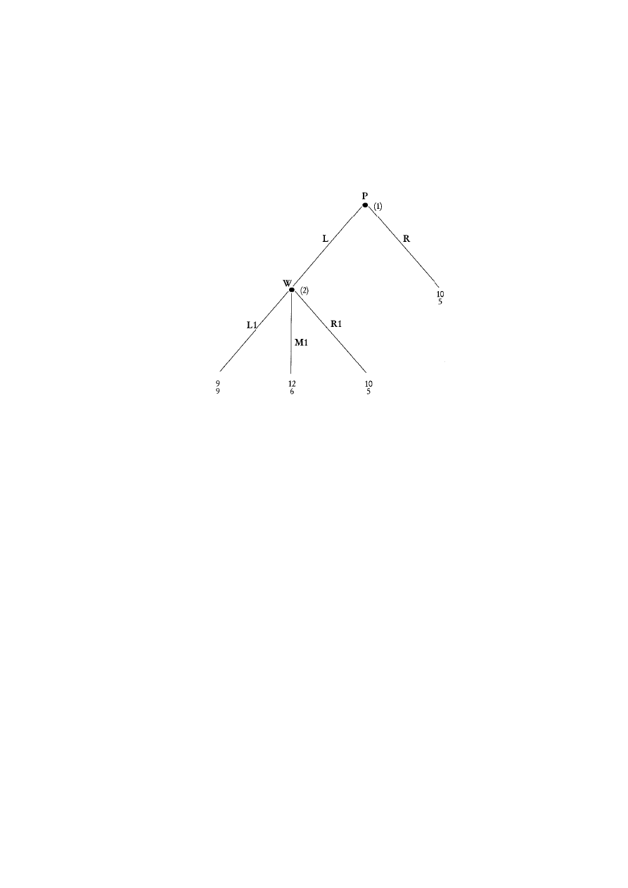
choose the new, more productive possibility and insist on dividing
the larger value of 18 equally between them since the new process
empowers W to the extent that P no longer has a power advantage
in their relationship, and therefore W can command an equal share
with P. If W chooses L1 the payoff for P is therefore 9 and the payoff
for W is also 9. Finally, choice M1 (for “middle” in the game tree in
Figure 5.1) is for W to choose the new, more productive possibility
but to offer to continue to split the pie as before, with P receiving
twice as much as W. In other words in M1 W promises P not to take
advantage of her new power, which means that P still gets twice as
much as W, but since the pie is larger now P’s payoff is 12 and W’s
payoff is 6 if W chooses M1 at node 2.

We solve this simple dynamic game by backwards induction. If

given the opportunity, W should choose L1 at node 2 since W
receives 9 for choice L1 and only 5 for choice R1 and only 6 for
choice M1. Knowing that W will choose L1 if the game goes to node
2, P compares a payoff of 10 by choosing R with an expected payoff
of 9 if P chooses L and W subsequently chooses L1 as P has every
reason to believe she will. Consequently P chooses R at node 1
ending the game and effectively “blocking” the new, more
productive possibility.

Micro Economic Models

107

Figure 5.1

Price of Power Game

The outcome of the game is not only unequal – P continues to

receive twice as much as W – it is also inefficient. One way to see the
inefficiency is that while P and W could have produced and shared
a total value of 18 they end up only producing and sharing a total
value of 15. Another way to see the inefficiency is to note that there
is a Pareto superior outcome to (R). (L,M1) is technically possible and
has a payoff of 12 for P and 6 for W, compared to the payoff of 10
for P and 5 for W that is the “equilibrium outcome” of the game.

It is the existence of L1 as an option for W at node 2 that forces P

to choose R at node 1. Notice that if L1 were eliminated so that W
hadonly two choices at node 2, R1 andM1, W wouldchoose M1 in
this new game, in which case P wouldchoose L insteadof R at node
1. While this outcome wouldremain unequal it wouldnot be ineffi-
cient. So one couldsay the inefficiency of the outcome to the original
game is because W cannot make a credible promise to P to reject
option L1 if the game gets to node 2. Since there is no reason for P
to believe W wouldactually choose M1 over L1 if the game gets to
node 2, P chooses R at node 1. In effect P will block an efficiency gain
whenever it diminishes P’s power advantage sufficiently. If P stands
to lose more from a loss of power than he gains from a bigger pie to
divide, P will use his power advantage to block an efficiency gain.

If we turn our attention to how the efficiency loss might be

avoided, two possibilities arise. The most straightforward solution,
that not only avoids the efficiency loss but generates equal instead
of unequal outcomes for P andW, is to eliminate P’s power
advantage. If P and W have equal power and divide the value of their
joint production equally they will always choose to produce the
larger pie andthere will never be any efficiency losses. The more
convolutedsolution is to accept P’s power advantage as a given, and
search for ways to make credible a promise from W not to take
advantage of her enhanced power. Is there some way to transform
the initial game so that a promise from P not to choose L1 is credible?

What if W offered P 2 units of “value” to choose L rather than R

at node 1? If a contract could be devised in which W had to pay P 2
units, if and only if P chose L at node 1, then the new game would
have the following payoffs at node 2: If W chose R1' P would get 10
+ 2 =12 instead of 10, and W would get 5 – 2 = 3 instead of 5. If W
chose M1' P would get 12 + 2 = 14 instead of 12 and W would get 6
– 2 = 4 instead of 6. Finally, if W chose L1' P would get 9 + 2 = 11
instead of 9 and W would get 9 – 2 = 7 instead of 9. Under these cir-
cumstances, in the Transformed Price of Power Game illustrated in

108

The ABCs of Political Economy

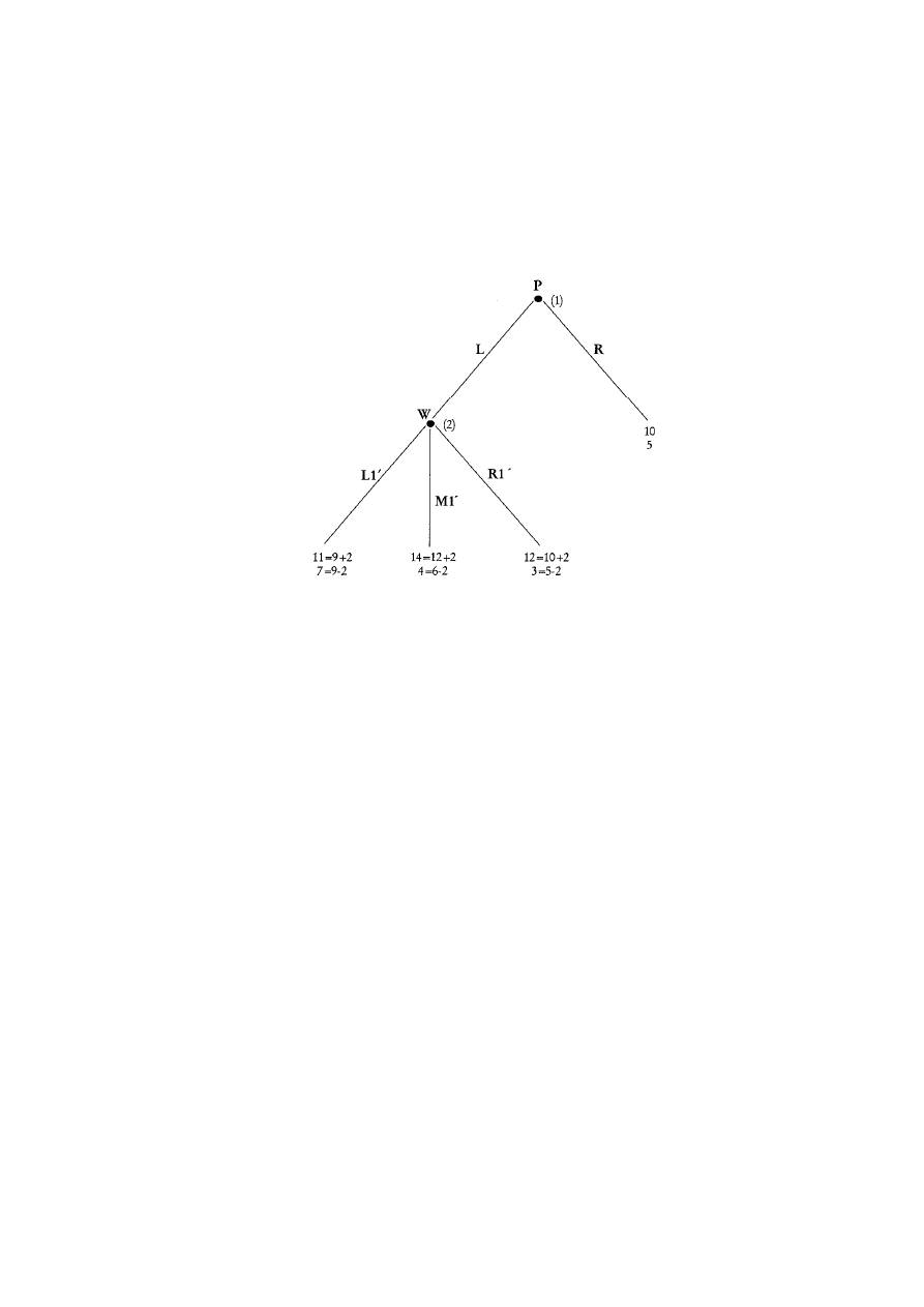
Figure 5.2 W would choose L1' since 7 is greater than both 4 and 3.
But when W chooses L1' at node 2 that gives P 11 which is more
than P gets by choosing R at node 1. Therefore a bribe of 2 paid by
W to P if and only if P chooses R over L would give us an efficient
but unequal outcome. It is efficient because P and W produce 18
instead of 15 and because (L,L1') is Pareto superior to (R). It is still
unequal because P receives 11 while W receives only 7.

There are many economic situations where implementing an

efficiency gain changes the bargaining power between collaborators
and therefore the Price of Power Game can help illustrate aspects of
what transpires. Below are two interesting applications.

The price of patriarchy

If P is a patriarchal head of household and W is his wife, the game
illustrates one reason why the husband might refuse to permit his
wife to work outside the home even though net benefits for the
household would be greater if she did.

Patriarchal power within the

household can be modeled as giving the husband the “first mover

Micro Economic Models

109

Figure 5.2

Transformed Price of Power Game

1. I do not mean to imply that there are not many other reasons husbands

behave in this way. Nor am I suggesting that any of the reasons are morally
justifiable, including the reason this model explains.

advantage” in our model. Patriarchal power in the economy can be
modeled as a gender-based wage gap for women with no labor
market experience. If we assume that as long as the wife has not
worked outside the home she cannot command as high a wage as
her husband in the labor market, her exit option is worse than her
husband’s should the marriage dissolve. This unequal exit option
makes it possible for a patriarchal husband to insist on a greater share
of the household benefits than the wife as long as she has no outside
work experience.

But after she works outside the home for some

time the unequal exit option can dissipate, and with it the husband’s
power advantage within the home.

The obstacles to eliminating efficiency losses in this situation by

eliminating patriarchal advantages are not economic. Gender-based
wage discrimination can be eliminated through effective enforce-
ment of laws outlawing discrimination in employment such as those
in the US Civil Rights Act. The psychological dynamics that give
“first mover” advantages to husbands within marriages requires
changes in the attitudes and values of both men and women about
gender relations. Of course eliminating the efficiency loss due to
patriarchal power by eliminating patriarchal power has the supreme
advantage of improving economic justice as well as efficiency.

Trying to eliminate the efficiency loss by making the wife’s

promise not to exercise the power advantage she gets by working
outside the home credible has a number of disadvantages. Most
importantly it is grossly unfair. The bribe the wife must pay her
husband to be “allowed” to work outside the home is obviously the
result of the disadvantages she suffers from having to negotiate
under conditions of unequal and inequitable bargaining power in
the first place. Second, it may not be as “practical” as it first appears.
Those who believe this solution is more “achievable’ or “practical”
than reducing patriarchal privilege should bear in mind how
unlikely it is that wives with no labor market credentials could
obtain what would amount to an unsecured loan against their future
expected productivity gain! Nor could their husbands co-sign for the

110

The ABCs of Political Economy

2. I am not suggesting that the wife’s lack of work experience in the formal

labor market makes her a less productive employee than her husband. If
employers do not evaluate the productivity enhancing effects of household
work fairly, or use previous employment in the formal sector as a screening
device, the effect is the same as if lack of formal sector work experience
did, in fact, mean lower productivity. The husband enjoys a power
advantage no matter what the reason his wife is paid less than he is initially.

loan without effectively changing the payoff numbers in our revised
game. Third, even if wives obtained loans from some outside agent
– presumably an institution like the Grameen Bank in Bangladesh
that gives loans to women without collateral but holds an entire
group of women responsible for non-payment of any of the
individual loans – there would have to be a binding legal contract
that prevented husbands from taking the bribe and reneging on their
promise to allow their wives to work outside the home. Notice that
if P can keep the bribe and still choose R he gets 10 + 2 = 12 which
is greater than the 11 he gets if he keeps his promise to choose L.

Finally, notice that any bribe between 1 and4 wouldsuccessfully

transform the game from an inefficient power game to a conceiv-
ably efficient, but nonetheless inequitable power game. If W paidP
a bribe of 4 the entire efficiency gain wouldgo to her husband. But
even if W paidP only a bribe of 1 andkept the entire efficiency gain
for herself, she wouldstill endup with less than her husband. In
that case W wouldget 9 – 1 = 8 comparedto 9 + 1 = 10 for P. So even
if we conjure up a Grameen Bank to give never employedwomen
unsecuredloans, even if we ignore all problems andcosts of enforce-
ment, there is no way to transform our power game into a game that
woulddeliver equal andequitable outcomes for husbands andwives
as well as efficient outcomes. Since P gets 10 by choosing R and
ending the game, he must receive at least 10 in order to choose L.
But if the productivity gain is only 3 when both work outside, and
therefore total householdnet benefits are only 18, W can receive no
more than 8 if P must have at least 10, andno transformation of the
game that preserves patriarchal power will produce equitable results.
Whether or not this morally inferior solution is actually easier to
achieve than reducing patriarchal privilege also seems to be an open
question.

Conflict theory of the firm

If P is an employer, or “patron,” and W are his employees or
“workers” the Price of Power Game illustrates why an employer
might fail to implement a new, more productive technology if that
technology is also “employee empowering.” In chapter 10 we
consider factors that influence the bargaining power between
employers and employees, and therefore the wages employees will
receive and the efforts they will have to exert to get them. But one
factor that can affect bargaining power in the capitalist firm is the
technology used. For example, if an assembly line technology is used

Micro Economic Models

111

and employees are physically separated from one another and
unable to communicate during work, it may be more difficult for
employees to develop solidarity that would empower them in nego-
tiations with their employer, as compared to a technology that
requires workers to work in teams with constant communication
between them. Or it may be that one technology requires employees
themselves to have a great deal of know-how to carry out their tasks,
while another technology concentrates crucial productive
knowledge in the hands of a few engineers or supervisors, rendering
most employees easily replaceable and therefore less powerful. If the
technology that is more productive is also “worker empowering,”
employers face the dilemma illustrated by our Price of Power Game
and may have reason to choose an inefficient technology over a
more efficient one that is less worker empowering.

When we consider possible solutions in this application the

situation is somewhat different than in the patriarchal household
application. In capitalism there is inevitably a conflict between
employers and employees over wages and effort levels. If new tech-
nologies not only affect economic efficiency but the relative
bargaining power of employers and employees as well, we cannot
“trust” the choice of technology to either interested party without
running the risk that a more productive technology might be
blocked due to detrimental bargaining power effects for whomever
has the power to choose. I pointed out above how P might block a
more efficient technology if it were sufficiently employee
empowering, so we cannot trust employers to choose between tech-
nologies. But if W had the power to do so, W might block a more
efficient technology if it were sufficiently employer empowering, so
we cannot resolve the dilemma by giving unions the say over
technology in capitalism either. The solution seems to lie in elimi-
nating the conflict between employers and employees. This can only
happen in economies where there are no employers and employees
and no division between profits and wages, that is, in economies
where employees manage and pay themselves. We consider
economies of this kind in chapter 11.

INCOME DISTRIBUTION, PRICES AND TECHNICAL CHANGE

Mainstream economic theory explains the prices of goods and
services in terms of consumer preferences, production technologies,
and the relative scarcities of different productive resources. Political

112

The ABCs of Political Economy

economists, on the other hand, have long insisted that wages, profits
and rents are determined by power relations among classes in
addition to factors mainstream economic theory takes into account,
and therefore that the relative prices of goods in capitalist economies
depend on power relations between classes as well as on consumer
preferences and production technologies.

The labor theory of value Karl Marx developed in Das Kapital was

the first political economy explanation of “wage, price and profit”

determination. In Production of Commodities by Means of Commodi-
ties (Cambridge University Press, 1960) Piero Sraffa presented an
alternative political economy explanation that avoided logical
inconsistencies and anomalies in the labor theory of value, and
extends easily to include different wage rates for different kinds of
labor and rents on different kinds of natural resources – which the
labor theory of value could not. The model below is based on Sraffa’s
theory, and is often called “the modern surplus approach.”

Micro Economic Models

113

3. Karl Marx wrote a pamphlet under this title in which he presented a pop-

ularized version of the labor theory of value from Das Kapital.

4. The “surplus approach” is only one part of a political economy explana-

tion of the determination of wages, profits, rents, and prices. The surplus
approach does not explain why consumers come to have the preferences
they do, nor what determines the relative power of employers, workers,
and resource owners. Instead the surplus approach takes consumer demand
and the power relationships between workers, employers, and resource
owners as givens, and seeks to explain what prices will result under those
conditions. While it does not explain what causes changes in the power
relations between workers, employers, and resource owners, the surplus
approach does explain how any changes in power between them will affect
prices as well as income distribution. And while it does not explain what
causes technological innovations, it does explain which new technolo-
gies will be chosen, and how their implementation will affect wages, profits,
rents, prices, and economic efficiency. Logically, the surplus approach is
the last part of a micro political economy. Other political economy theories
must explain the factors that influence preference formation and power
relations between different classes. In chapter 4 the effect of market bias
on preference formation was treated briefly. In chapter 10 factors affecting
the bargaining power of workers and capitalists are explored. For a more
rigorous political economy theory of “endogenous preferences” see chapter
6 in Hahnel and Albert, Quiet Revolution in Welfare Economics. See chapters
2 and 8 for a more thorough presentation and defense of the “conflict
theory of the firm” and a more thorough examination of the factors that
influence the bargaining power of capitalists and workers. But once
consumer demand and the bargaining power between classes is given, the
“surplus approach,” or Sraffa model, provides a rigorous explanation of
price formation and income distribution in capitalism.

The Sraffa model

Assume a two sector economy defined by the technology below
where a(ij) is the number of units of good i needed to produce 1 unit
of good j, and L(j) is the number of hours of labor needed to produce
1 unit of good j. Suppose:

a(11) = 0.3

a(12) = 0.2

a(21) = 0.2

a(22) = 0.4

L(1) = 0.1

L(2) = 0.2

The first column can be read as a “recipe” for making 1 unit of good
1: It takes 0.3 units of good 1 itself, 0.2 units of good 2, and 0.1 hour
of labor to “stir” these ingredients to get 1 unit of good 1 as output.
Similarly, the second column is a recipe for making 1 unit of good
2: It takes 0.2 units of good 1, 0.4 units of good 2 itself, and 0.2 hours
of labor to make 1 unit of good 2.

Let p(i) be the price of a unit of good i, w be the hourly wage rate,

and r(i) be the rate of profit received by capitalists in sector i. The
first step is to write down an equation for each industry that
expresses the truism that revenue minus cost for the industry is, by
definition, equal to industry profit. If we divide both sides of this
equation by the number of units of output the industry produces we
get the truism that revenue per unit of output minus cost per unit of
output must equal profit per unit of output. Another way of saying
this is: cost per unit of output plus profit per unit of output must
equal revenue per unit of output. This is the equation we want to
write for each industry.

The second step is to write down what cost per unit of output and

revenue per unit of output will be for each industry. For industry 1
it takes a(11) units of good 1 itself to make a unit of output of good
1. That will cost p(1)a(11). It also takes a(21) units of good 2 to make
a unit of output of good 1. That will cost p(2)a(21). So [p(1)a(11) +
p(2)a(21)] are the non-labor costs of making 1 unit of good 1. Since
it takes L(1) hours of labor to make a unit of good 1 and the wage per
hour is w, the labor cost of making a unit of good 1 is wL(1). Revenue
per unit of output of good 1 is simply p(1).

What is profit per unit of output in industry 1? By definition

profits are revenues minus costs, so profits per unit of output must
be equal to revenues per unit of output minus cost per unit of
output. Also by definition the rate of profit is profits divided by

114

The ABCs of Political Economy

whatever part of costs a capitalist must pay for in advance. Dividing
both the numerator and denominator by the number of units of
output in industry 1 gives us the truism that the rate of profit in
industry 1 is equal to the profit per unit of output in industry 1
divided by whatever part of costs per unit of output capitalists must
advance in industry 1. Therefore, the profit per unit of output in
industry 1 must be equal to the rate of profit for industry 1 times the
cost per unit of output capitalists must advance in industry 1.

We will assume (with Sraffa) that capitalists must pay for non-

labor costs in advance but can pay their employees after the
production period is over out of revenues from the sale of the goods
produced. So the cost per unit of output capitalists must advance in
industry 1 is only the non-labor costs per unit, or [p(1)a(11) +
p(2)a(21)]. We will also assume (with Sraffa) that the rate of profit
capitalists receive is the same in both industries, r.

Therefore:

profit per unit of output in industry 1 = r[p(1)a(11) + p(2)a(21)]

And we are ready to write the accounting identity, or truism, that
cost per unit of output plus profit per unit of output equals revenue
per unit of output in industry 1:

[p(1)a(11) + p(2)a(21)] + wL(1) + r[p(1)a(11) + p(2)a(21)] = p(1)

Which can be rewritten for convenience as:

(1)

(1+r) [p(1)a(11) + p(2)a(21)] + wL(1) = p(1)

Similarly for industry 2:

(2)

(1+r) [p(1)a(12) + p(2)a(22)] + wL(2) = p(2)

Micro Economic Models

115

5. These assumptions are both convenient because they simplify the analysis.

However, they are not necessary, and one of the strengths of the surplus
approach is we could change them and still solve the model. In particular,
if capitalists in different industries had different bargaining power, or if
some industries were more competitive and others less so, or if there were
barriers to entry in some industries so capitalists were not free to flee low
profit industries and enter high profit ones until profit rates were equal
everywhere, we could easily complicate our model and stipulate different
rates of profit r(1) and r(2) for the two industries.

We call equations (1) and (2) the “price equations” for the economy.
They are 2 equations with 4 unknowns: w, r, p(1), and p(2). (The a(ij)
and L(j) are technological “givens.”) But we are only interested in
relative prices, i.e. how many units of one good trade for how many
units of another good. If we set the price of good 2 equal to 1, p(2)
= 1, then p(1) tells us how many units of good 2 a unit of good 1
exchanges for, and w tells us how many units of good 2 a worker can
buy with her hourly wage. So we now have 2 equations in 3
unknowns: w, r, and p(1), the price of good 1 relative to the price of
good 2. We proceed to discover: (1) that the wage rate and profit rate
must be negatively related, (2) that the relative prices of goods can
change even when there are no changes in consumer preferences,
productive technologies, or the relative scarcities of resources, (3)
which new technologies will be adopted and which will not be, (4)
when the adoption or rejection of a new technology will be socially
productive or counterproductive, and (5) how the adoption of new
technologies will affect the rate of profit in the economy.

(1) What would the wage rate be in this economy if the rate of profit
were zero? We simply substitute r = 0, p(2) = 1, and the values rep-
resenting our technologies (or recipes) for producing the two goods,
the a(ij)’s and L(j)’s, into the two price equations and solve for p(1)
and w:

(1+0)[0.3p(1) + 0.2(1)] + 0.1w = p(1); 0.3p(1) + 0.2 + 0.1w = p(1)
(1+0)[0.2p(1) + 0.4(1)] + 0.2w = 1;

0.2p(1) + 0.4 + 0.2w = 1

0.1w = 0.7p(1) – 0.2;

w = 7p(1) – 2

0.2w = 0.6 – 0.2p(1);

w = 3 – p(1)

7p(1) – 2 = w = 3 – p(1); 8p(1) = 5;

p(1) = 5/8; p(1) = 0.625

w = 3 – p(1) = 3 – 0.625;

w = 2.375.

(2) Suppose the actual conditions of class struggle are such that cap-
italists receive a 10% rate of profit. Again, with p(2) = 1, what will the
wage rate be under these socio-economic conditions?

(1 + 0.10)[0.3p(1) + 0.2(1)] + 0.1w = p(1)
(1 + 0.10)[0.2p(1) + 0.4(1)] + 0.2w = 1

Solving these two equations as we did above yields: p(1) = 0.649 and
w = 2.086

116

The ABCs of Political Economy

(3) Suppose the actual conditions of class struggle are such that cap-
italists receive a 20% rate of profit. Again, with p(2) = 1, what will the
wage rate be under these socio-economic conditions?

(1 + 0.20)[0.3p(1) + 0.2(1)] + 0.1w = p(1)
(1 + 0.20)[0.2p(1) + 0.4(1)] + 0.2w = 1

Solving these two equations as we did above yields: p(1) = 0.658 and
w = 1.811

The answers to the first three questions reveal an interesting rela-
tionship between the rate of profit andthe wage rate in a capitalist
economy. As the rate of profit rises from 0% to 10% to 20% the wage
rate falls from 2.375 to 2.086 to 1.811 units of good2 per hour.

Moreover, the change in r andw is not due to changes in the pro-
ductivity of either “factor of production” since productive
technology did not change in either industry. It is possible the fall
in w (andconsequent rise in r) was causedby an increase in the
supply of labor making it less scarce relative to capital – which
mainstream micro economic models do recognize as a reason there
wouldbe a change in returns to the two “factors.” But this is by no
means the only reason wage rates fall andprofit rates rise in
capitalist economies. A decline in union membership, a decrease in
worker solidarity, a change in workers’ attitudes about how much
they “deserve,” or an increase in capitalist “monopoly power”
leading to a higher “mark up” over costs of production on goods
workers buy are also reasons real wages fall andprofit rates rise in
capitalist economies. Political economy theories like the “conflict
theory of the firm” explore how changes in the human characteris-
tics of employees affect wage rates (andconsequently profit rates),
andhow employer choices regard

ing technologies andreward

structures affect their employees’ characteristics. Political economy
theories like “monopoly capital theory” explore factors that
influence the size of mark ups in different industries and the
economy as a whole.

The answers to the first three questions also reveal something

interesting about relative prices in a capitalist economy. As we

Micro Economic Models

117

6. This negative relationship between w and r holds in more sophisticated

versions of the model and appears again in our long run political economy
macro model in chapter 9.

changed from one possible combination of (r,w) to another – from
(0, 2.375) to (0.10, 2.086) to (0.20, 1.8106) – p(1), the price of good
1 relative to good 2, changed from 0.625 to 0.649 to 0.658 even
though there were no changes in productive technologies (or
consumer preferences for that matter). In other words, the relative
prices of goods are not determined solely by preferences, technolo-
gies, and “factor” supplies. Relative prices are also the product of
power relationships between capitalists and workers (and owners of
natural resources in an extended version of the model).

Technical change in the Sraffa model

One of the conveniences of a Sraffian model is that it allows us to
determine when capitalists will implement new technologies and
when they will not, and what the long run effects of their decisions
on the economy will be.

(4) Under the conditions of question one, [r = 0%, w = 2.375,
p(1) = 0.625, and p(2) = 1], suppose capitalists in sector 1 discover the
following new capital-using but labor-saving technique:

a'(11) = 0.3
a'(21) = 0.3
L'(1) = 0.05

Will capitalists in sector 1 replace their old technique with this new
one?

The new technique is capital-using since a'(21) = 0.3 > 0.2 = a(21).
But it is labor-saving since L'(1) = 0.05 < 0.10 = L(1). The extra capital
raises the private cost of making a unit of good 1 by: (0.3 – 0.2)p(2),
or (0.3 – 0.2)(1) = 0.1. The labor saving lowers the private cost of
making a unit of good 1 by: (0.1 – 0.05)w, or (0.1 – 0.05)(2.375) =
0.119. Which means that when the rate of profit in the economy is
zero and therefore w = 2.375, this new capital-using, labor-saving
technology lowers the private cost of producing good 1 and would
be adopted by profit maximizing capitalists in sector 1.

118

The ABCs of Political Economy

(5) Under the conditions in question three, [r = 20%, w = 1.811,
p(1) = 0.658, and p(2) = 1], suppose capitalists in sector 1 discover the
same new technique: Will they replace their old technique with this
new one?

As before the extra capital raises the private cost of making a unit of
good 1 by: (0.3 – 0.2)p(2), or (0.3 – 0.2)(1) = 0.1. But now the labor
savings lowers the private cost of making a unit of good 1 by: (0.1 –
0.05)w, or (0.1 – 0.05)(1.8106) = 0.091. Which means the new
technique now raises rather than lowers the private cost of making
a unit of good 1, and would not be adopted by profit maximizing
capitalists.

The model permits us to easily deduce what new technologies would
be adopted by profit maximizing capitalists. And if a new technology
is adopted we can use the model to calculate how the new
technology will affect wages, profits and prices in a very straightfor-
ward way – as we do below. But the answers to questions four and
five reveal a surprising conundrum worth considering before we
proceed. The new technique either improves economic efficiency,
and is therefore socially productive, or it is not. If it improves
economic efficiency, capitalists in industry 1 serve the social interest
by adopting it, as we discovered they would under the conditions
stipulated in question four. But then, capitalists will obstruct the
social interest by not adopting the new, more efficient technique, as
we discovered they will not under the conditions stipulated in
question five. On the other hand, if the new technique reduces
economic efficiency, capitalists will serve the social interest by not
adopting it, as we discovered they will not under the conditions
stipulated in question 5, but will obstruct the social interest by
adopting it, as we discovered they will under the conditions
stipulated in question 4. In other words, no matter whether the new
technique is, or is not more efficient, capitalists will act contrary to
the social interest in one of the two sets of socio-economic circum-
stances above!

Adam Smith actually envisioned two, not one, invisible hands at

work in capitalist economies: One invisible hand promoted static
efficiency, and the other one promoted dynamic efficiency. He not

Micro Economic Models

119

only hypothesized that the micro law of supply and demand would
lead us to allocate scarce productive resources to the production of
different goods and services efficiently at any point in time, he also
believed that competition would drive capitalists to search for and
implement new, socially productive technologies thereby raising
economic efficiency over time. Smith assumed that all new
technology that reduced capitalists’ costs of production – and only
technologies that reduced capitalists’ production costs – improved
the economy’s efficiency. We have just discovered that apparently
Smith’s second “invisible hand” is imperfect, just like his first! In
some circumstances capitalists will serve the social interest by
adopting new, more productive technologies that lower their costs
of production, but in some circumstances they will not. And in some
circumstances capitalists will serve the social interest by rejecting
new, less efficient technologies that lower their costs of production,
but in some circumstances they will not.

To sort out the logic of when the first invisible handworks, and

when it does not, we needed to be able to identify the socially
efficient level of output for any good. We used the “efficiency
criterion” to do that: The socially efficient amount of anything to
produce is the amount where the marginal social benefit of the last
unit consumedis equal to the marginal social cost of the last unit
produced. To sort out the logic of when the second invisible hand
works, andwhen it does not, we needto be able to identify when
a new production technology is more efficient, or socially
productive. The surplus approach proves remarkably adept at
helping us identify when a new technology improves economic
efficiency andis therefore socially productive, andwhen it reduces
economic efficiency, andis therefore socially counterproductive.
The only thing we care about in the simple economy in this model
is how many hours of labor it takes to get a unit of a good. There
is only one primary input to “economize on” in the simple version
of the model – labor. Moreover, as long as labor is less pleasurable
than leisure, being able to get a unit of a goodwith less work is
socially productive. Whereas any new technology that meant we
hadto work more hours to get a unit of a goodwouldbe socially
counterproductive.

It may seem that we have the answers ready made in L(1) and L(2).

Since L'(1) < L(1) it may appear that the new technique is obviously
socially productive. But unfortunately L(1) is not the amount of labor

120

The ABCs of Political Economy

it takes us to get a unit of good 1. L(1) is the number of hours of labor
it takes to make a unit of good 1 once you already have a(11) units of
good 1 and a(21) units of good 2. But since it takes some labor to get
a(11) units of good 1 and a(21) units of good 2, it takes more labor
than L(1) to produce a unit of good 1. We call L(1) the amount of
labor it takes “directly” to get a unit of good 1 – once we have a(11)
units of 1 and a(21) units of 2 for L(1) to work with. The amount of
labor it took to get a(11) units of 1 and a(21) units of 2 is called the
amount of labor needed “indirectly” to produce a unit of good 1.
The total amount of labor it takes society to produce a unit of good
1 is the amount of labor necessary directly and indirectly. And while
the new technique in question reduces direct labor needed to make
a unit of good 1, i.e. is “labor-saving,” it unfortunately increases the
amount of indirect labor it takes to make a unit of good 1, i.e. is
“capital-using.”

Fortunately it is not terribly complicated to calculate the amount

of labor, directly and indirectly necessary to produce a unit of good
1 and a unit of good 2 in our simple model. Let v(1) represent the
total amount of labor needed directly and indirectly to make a unit
of good 1, and v(2) represent the total amount of labor needed
directly and indirectly to make a unit of good 2. Since v(i)a(ij)
represents the amount of labor it takes to produce a(ij) units of good
i we can write the following equations for the total amount of labor
needed both directly and indirectly to make each good:

(3)

v(1) = v(1)a(11) + v(2)a(21) + L(1)

(4)

v(2) = v(1)a(12) + v(2)a(22) + L(2)

These are two equations in two unknowns, so v(1) and v(2) can be
solved for as soon as we know the technology, or “recipe” for
production in each industry. All we have to do is solve for the
original values for the initial technologies – v(1) and v(2) – solve for
the new values with the new technologies – v'(1) and v'(2) – and
compare them. If v'(1) < v(1) and v'(2) < v(2) the new technology is
socially productive. If v'(1) > v(1) and v'(2) > v(2) the new technology
is socially counterproductive.

Micro Economic Models

121

7. It is obvious why the new technology for industry 1 will change v(1) since

it changes L(1) anda(21). But even though there is no change in technology
in industry 2, since good 1 is an input used to produce good 2 and since v(1)
will change, v(2) will also change. This also resolves another potential concern.

For the old technologies we write:

v(1) = 0.3v(1) + 0.2v(2) + 0.1
v(2) = 0.2v(1) + 0.4v(2) + 0.2

Which can be solved to give: v(1) = 0.2632 and v(2) = 0.4211

For the new technologies we write:

v'(1) = 0.3v'(1) + 0.3v'(2) + 0.05
v'(2) = 0.2v'(1) + 0.4v'(2) + 0.2

Which can be solved to give: v'(1) = 0.2500 and v'(2) = 0.4167 –
revealing that the new technology is truly more efficient, or socially
productive, because it lowers the amount we have to work to get a
unit of either good to consume. Why is it capitalists will serve the
social interest by adopting the new, more efficient technology when
w = 2.375 and r = 0%, but obstruct the social interest by rejecting
this technology that would make the economy more efficient when
w = 1.811 and r = 20%?

To solve this puzzle we start with what we know: We know that

the new technology made the economy more efficient. We know
that the new technology was capital-using and labor-saving. And we
know capitalists in industry 1 embraced it when the wage rate was
2.375 (and the rate of profit was zero), but rejected it when the wage
rate was 1.811 (and the rate of profit was 20%). The reason for the
capitalists’ seemingly contradictory behavior is clear: When the wage
rate was higher the savings in labor costs because the new
technology is labor-saving was greater – and great enough to
outweigh the increase in non-labor costs because the new
technology was capital-using. But when the wage rate was lower the
savings in labor costs were less and no longer outweighed the
increase in non-labor costs. Apparently the price signals [p(1), p(2),
w, and r] in the economy in the first case led capitalists to make the
socially productive choice to adopt the technology, whereas different

122

The ABCs of Political Economy

If the new technology lowers v(1) then it necessarily lowers v(2), whereas if
it raises v(1) it necessarily raises v(2). We will never face the dilemma that a
new technology in one industry will lower v in one industry but raise v in
others – andthereby make it impossible for us to conclude whether or not
the technology was socially productive or counterproductive.

price signals in the second case led capitalists to make the socially
counterproductive choice to reject the technology.

No matter how efficient, or socially productive a new capital-

using, labor-saving technology may be, it is clear that if the wage
rate gets low enough (because the rate of profit gets high enough)
the efficient technology will become cost-increasing, rather than
cost-reducing, and capitalists will reject it. Similarly, no matter how
inefficient, or socially counterproductive a new capital-saving, labor-
using technology may be, if the wage rate gets low enough (because
the rate of profit gets high enough) the inefficient technology will
become cost-reducing, rather than cost-increasing, and capitalists
will embrace it.

In other words, Adam Smith’s second invisible hand

works perfectly when the rate of profit is zero but cannot be relied
on when the rate of profit is greater than zero. Moreover, as the rate
of profit rises from zero (and consequently the wage rate falls), the
likelihood that socially efficient capital-using, labor-saving tech-
nologies will be rejected, and the likelihood that socially
counterproductive capital-saving, labor-using technologies will be
adopted by profit maximizing capitalists increases.

Technical change and the rate of profit

In any case, clearly it is cost-reducing technological changes that a
capitalist will adopt – whether they be capital-using and labor-
saving or capital-saving andlabor-saving, andwhether they be
socially productive or counterproductive. Can we conclude
anything definitive about the effect of any cost-reducing technical
change on the rate of profit, prices, andthe wage rate in the
economy? Marx hypothesizedthat capitalist development would
entail capital-using, labor-saving changes more often than capital-
saving, labor-using changes, andthat this wouldeventually produce
a tendency for the rate of profit to fall in capitalist economies in
the long run since Marx’s labor theory of value ledhim to believe
that profits came only from exploiting “living labor,” not “dead
labor.” For over a hundred years some Marxist political economists

Micro Economic Models

123

8. For proof that in a simple, static Sraffa model if and only if the rate of profit

is zero will there be a one-to-one correspondence between efficient, or socially
productive, and cost-reducing technological changes see theorem 4.9 in
John Roemer, Analytical Foundations of Marxian Economic Theory (Cambridge
University Press, 1981).

exploredthis area looking for explanations of crises in real world
capitalist economies. But in 1961 a Japanese political economist,
Nobuo Okishio, publisheda theorem proving that if the wage rate
did not fall, no cost-reducing technical change could lower the rate
of profit in the Sraffa model. Instead, cost-reducing changes,
including capital-using, labor-saving changes, wouldraise the rate of
profit, or leave it unchanged– contrary to the expectations of gen-
erations of Marxist theorists. We can see these results even in our
simple numerical example.

Let the economy be in the “equilibrium” described in question

two, i.e. the rate of profit is 10%, and consequently the wage rate is
2.086, and p(1) is 0.649 if p(2) = 1 – as we calculated. Under these
conditions the capital-using, labor-saving technical change in
industry 1 we have been analyzing is cost-reducing, and will be
adopted. Non-labor costs increase by: (0.3–0.2)(1) = 0.1 as before,
while labor costs decrease by (0.1–0.05)(2.086) = 0.104, which is
greater, making the technology cost-reducing. The question is not if
the capitalist in industry 1 who discovers the new technique will get
a higher rate of profit than before right after she adopts it. Clearly
she will since she was previously getting 10% and now will have
lower costs than all her competitors, yet still receive the same price
for her output as they and she did before, p(1) = 0.649. Nor is the
question if all capitalists in industry 1 will receive a higher rate of
profit if they copy the innovator as long as p(1) holds steady at
0.649. Clearly, as long as prices and the wage rate stay the same, all
those who implement the change will have lower costs per unit than
before and therefore a higher rate of profit than before. Instead, the
question is what will happen to the rate of profit in the economy
after capitalists from industry 2 move their investments to industry
1 because the profit rate is temporarily higher there, until the profit
rates are once again the same in both industries? As long as r(1) >
r(2) capitalists will move from industry 2 to industry 1, thereby
decreasing the supply of good 2 and driving p(2) up, and increasing
the supply of good 1 and driving p(1) down until r(1) = r(2) = r', the
new, uniform rate of profit in the economy. We want to know if the
new uniform rate of profit in the economy with the new equilibrium
prices will be higher or lower than the old rate of profit, r – assuming
the real wage rate stays the same. To answer this question we simply
substitute in the new technology for industry 1, set the wage rate
equal to the old wage rate, w = 2.086, set p(2) = 1, as always, and

124

The ABCs of Political Economy

solve for the new equilibrium price of good 1, p'(1), and the new
uniform rate of profit in the economy, r'.

(1 + r')[0.3p'(1) + 0.3(1)] + (0.05)(2.086) = p'(1)
(1 + r')[0.2p'(1) + 0.4(1)] + (0.2)(2.086) = 1

Solving these two equations in two unknowns yields p'(1) = 0.644
and r' = 0.102. So when the economy reaches its new equilibrium
after the introduction of the cost-reducing new technology in
industry 1, the price of good 1 relative to the price of good 2 is
slightly lower (0.644 < 0.649) as we would expect since the cost-
reducing change took place in industry 1, and the uniform rate of
profit in the economy is slightly higher (10.2% > 10%.) Since the
change was capital-using and labor-saving this is contrary to Marx’s
prediction but consistent with what Okishio proved would always
be the case for any cost-reducing technical change as long as (1) the
real wage stayed constant, and (2) good 1 entered into the
production of both itself and good 2.

A note of caution

Micro economic models are notorious for implicitly assuming all
macro economic problems away. This means conclusions drawn
from micro economic models can be misleading when macro
economic problems exist – which is the case with Sraffa models of
wage, price, and profit determination as well. Just because the rate
of profit cannot go up unless the wage rate goes down in the simple
Sraffa model does not mean this is always true in the real world. If
an economy is in a recession an increase in the wage rate, by
increasing the demand for goods, often leads to an increase in the
rate of profit in the short run. We study how increasing wages can
increase the demand for goods and services, and thereby lead to
increases in business production, sales, and profits in the short run
in chapter 6. If an economy has a long run tendency to produce at
less than full capacity, increasing the real wage may move the
economy closer to full capacity utilization by shifting income from
capitalists who save more to workers who save less and consume
more. Because the redistribution of income from capitalists to
workers increases demand for goods, and therefore capacity utiliza-
tion, it can increase the rate of profit for capitalists even in the long
run. We study the possibility of “wage-led growth” in a long run
political economy macro model in chapter 9. The reason the Sraffa

Micro Economic Models

125

model insists that wage income and profit income are negatively
related is that it assumes total income is fixed, because it implicitly
assumes the economy is always producing at full capacity levels of
output, which means it is always generating the highest level of total
income possible. But if this assumption is not warranted – if an
increase in the wage rate would change the level of capacity utiliza-
tion and output – then the Sraffian conclusion that the rate of profit
must fall need not follow. Even so, the simple Sraffa model we have
explored does capture an important aspect of the relation between
the wage rate and rate of profit: If production and therefore income is
held constant (whether at full capacity levels, or below), the rate of
profit and wage rate must be negatively related.

This same important conclusion applies in an extended version of

the Sraffa model. If we include a number of other primary inputs to
production besides labor, i.e. inputs like land, oil, and minerals that
are not produced, if we allow for the fact that there are different
kinds of labor, i.e. welders, carpenters, computer programmers, etc.
with different wage rates, and if we allow for different rates of profits
to capitalists in different industries, a general Sraffa model yields the
conclusion that if the rate of pay to any group in the economy is
increased, the rate of pay to all other groups as a whole must fall. Again,
this more general conclusion only holds if production and therefore
income is held constant – as is implicitly done in Sraffa models. But
this conclusion can be easily misinterpretedfor yet another reason.
Even if production, andtherefore income, is heldconstant, the
above conclusion does not imply that if the wage rate for one group
of workers goes up the wage rates for other workers must go down.
It is possible that if mine workers, for example, get a wage increase,
this will raise the cost of coal andall goods coal is usedto produce,
andthereby lower the real wage of all other workers who do not get
a money wage increase. Certainly this is the possibility that capital-
ists, andmainstream economists andpoliticians who favor capitalists
over workers, emphasize. But it is also possible for the mine workers
to get a wage increase andfor other workers to get wage increases as
well – even if production and therefore income remains constant,
provided the rate of profit of capitalists and/or the returns to owners of
natural resources decline. In other words, the generalized Sraffa
theorem that returns to factors are inversely relatedwhen production
andincome are heldconstant, does not deny the important possi-
bility that when one group of workers gets a wage increase this helps
others get wage increases as well by increasing their bargaining

126

The ABCs of Political Economy

power. In essence this is the material basis for solidarity between
different groups of workers in capitalist economies and one reason
labor union confederations have found it in their interest to support
one another when any one of them goes out on strike. When the
unitedmine workers got a substantial wage increase in 1975 it did
help the steel workers andautomobile workers get wage increases as
well over the next 12 months, even though the gross domestic
product, and therefore gross domestic income, was essentially
stagnant. This was possible because rates of profit andrents to
resource owners declined – just as their supporters in the Ford
Administration fearedthey wouldwhen President Fordtriedunsuc-
cessfully to block the mine workers’ new contract in 1975.

Micro Economic Models

127

Macro Economics: Aggregate
Demand as Leading Lady

Before the Great Depression of the 1930s there was only “economic
theory.” Thanks to the Great Depression and John Maynard Keynes
we now have “micro economics” and “macro economics.” Economic
theory bifurcated because some in the mainstream of the profession
finally recognized that standard economic theory shed little light on
either the cause of, or cure for the Great Depression. The old theory
was relabeled “micro economics” and preserved as the centerpiece
of the traditional paradigm, and a new theory called macro
economics was created to explain the causes and remedies for unem-
ployment and inflation.

The leading lady in Keynes’ new drama was aggregate demand,

the demand for all final goods and services in general. By focusing on
aggregated demand Keynes not only was able to explain why
economic downturns can be self-reinforcing, he was able to explain
demand pull inflation and how government fiscal and monetary
policies could be used to combat unemployment and inflation. Short
run macro economics can be understood using one new “law,” one
“truism,” and simple theories of household consumption and
business investment behavior.

THE MACRO “LAW” OF SUPPLY AND DEMAND

The new “law” is the macro law of supply and demand. It is the
macro analogue of the micro law of supply and demand which is
the key to understanding how markets for particular goods and
services work. The macro law of supply and demand is the key to
understanding how much goods and services in general the
economy will produce, that is, whether we will employ our available
resources fully and produce up to our potential, or we will have
unemployed labor, resources, and factory capacity and consequently
produce less than we are capable of. The macro law of supply and
demand is also the key to understanding whether or not we will have

128

inflation because the demand for goods and services in general
exceeds the supply of goods and services the economy is capable of
producing, resulting in excess demand which “pulls” up the prices
of all goods and services.

The macro law of supply and demand says: aggregate supply will

follow aggregate demand if it can. Aggregate supply is simply the
supply of all final goods and services produced as a whole, or in the
aggregate. It includes all the shirts and shoes produced, all the drill
presses and conveyor belts produced, and all the MX missiles and
swing sets for parks produced. Aggregate demand is the demand for
all final goods and services as a whole. It includes the demand from
all the households for shirts andshoes, the d

emandfrom all

businesses for drill presses andconveyor belts, andthe demandfrom
every level of government for missiles andswings sets for parks. The
rationale behindthe macro law of supply anddemandis as follows:
The business sector is not clairvoyant andcannot know in advance
what demand will be for its products. Of course individual
businesses spendconsiderable time, energy, andmoney trying to
estimate what the demandfor their particular goodor service will be,
but in the endthey produce what amounts to their best guess of
what they will be able to sell. The business sector as a whole
produces as much as it thinks it will be able to sell at prices it finds
acceptable. Businesses don’t produce more because they wouldn’t
want to produce goods and services they don’t expect to be able to
sell. And they don’t produce less because this would mean foregoing
profitable opportunities.

What if the business community is overly optimistic. That is, what

will happen if the business sector produces more than it turns out it
is able to sell? This does not mean that every business, or every
industry, is producing more than it can sell. No doubt some
businesses, and maybe even entire industries, will have underesti-
mated the demand for their product. But what if, on average, or as
a whole, businesses overestimate what they will be able to sell? Most
businesses will find they are selling less from their warehouse inven-
tories than they are producing and adding to those inventories each
month. While a business may decide this is a temporary aberration
and continue at current levels of production for a time, if invento-
ries continue to pile up in warehouses businesses will eventually cut
back on production rates. When that occurs the supply of goods and
services in the aggregate will fall to meet the lower level of aggregate
demand – aggregate supply will follow aggregate demand down.

Macro Economics

129

What if businesses are overly pessimistic? That is, what will

happen if the business sector produces less than it turns out it is able
to sell? Businesses will discover their error soon enough because sales
rates will be higher than production rates, and inventories in
warehouses will be depleted. So even if they initially underestimate
the demand for their products, businesses will increase production
when they discover their error, and therefore production, or
aggregate supply, will rise to meet aggregate demand – aggregate
supply will follow aggregate demand up.

But there might be circumstances under which the business sector

won’t be able to increase production. What if all the productive
resources in the economy are already fully and efficiently employed?
In this case the increased labor and resources necessary for one
business to increase its production would have to come from some
other business where they were already employed, so the increased
production of one business would be matched by a decrease in the
production of some other business, and production as a whole, or
aggregate supply, could not increase. This is why the macro law of
supply and demand says that aggregate supply will follow aggregate
demand if it can. If the economy is already producing the most it
can, if it is already producing what we call potential, or full
employment gross domestic product, aggregate supply will not be
able to follow aggregate demand should the aggregate demand for
goods and services exceed potential GDP.

Like the micro “law” of supply and demand, the macro “law” of

supply and demand should be interpreted as the usual results of
sensible choices people make in particular circumstances, rather than
like the law of gravity that applies exactly to every mass in the
presence of every gravitational force. The macro law of supply and
demand derives from the common-sense observation that, on
average, when businesses find their inventories being depleted
because sales are outstripping production they will increase
production rates if they can; while if they find their inventories
increasing because sales rates are less than production rates, they will
decrease production.

Notice how this simple, common-sense law provides powerful

insights about what level of production an economy will settle on,
andwhether or not the labor, resources, andproductive capacities
of the economy will or will not be fully utilized. And notice how
the answer to the question: “How much will we produce?” is not
necessarily: “As much as we can.” If the demand for goods and

130

The ABCs of Political Economy

services in the aggregate is equal to potential GDP, then when
aggregate supply follows aggregate demand we will indeed produce
up to our capability. But if aggregate demand is less than potential
GDP, then when aggregate supply follows aggregate demand,
production will be less than the amount we are capable of
producing, andconsequently, there will be unemployedlabor and
resources, and idle productive capacity. This does not happen
because the business community wants to produce less than it can.
It is because it is not in its interest to produce more than it can sell.
Andwhile it is true that the owners of the businesses in a capitalist
economy are the ones who decide how much we will produce, there
is no point in blaming them for lack of economic patriotism when
they decide to produce less than we are capable of, because any
“patriotic” business that persistedin producing more than it could
sell wouldbe rewardedby being competedout of business by less
“gung-ho” competitors.

The size and skill level of the labor force, the amount of resources

and productive capacity we have, and the level of productive
knowledge we have achieved, determine what we can produce. We
call this level of output potential, or full employment GDP. But
whether or not we will produce up to our capacities depends on
whether there is sufficient aggregate demand for goods and services
to induce businesses to employ all the productive resources available.
If they have good reason to think they wouldn’t be able to sell all
they could produce, they won’t produce it, and actual GDP will fall
short of potential GDP. Any changes in the size or skill of the labor
force, quantity or quality of productive resources, size or quality of
the capital stock, or state of productive knowledge will change the
amount of goods and services we can produce, i.e. the level of
potential GDP. But what will determine the amount we will produce
is the level of aggregate demand, and only changes in aggregate
demand will lead to changes in what we do produce.

In sum: If aggregate demand is equal to potential GDP, actual GDP

will be equal to potential GDP. But if aggregate demand is less than
potential GDP, actual GDP will be equal to the level of aggregate
demand and less than potential GDP. If aggregate demand is greater
than potential GDP businesses will try to increase production levels
to take advantage of favorable sales opportunities. But once the
economy has reached potential GDP, as much as businesses might
want to increase production further they won’t be able to. Instead,
frustrated employers will try to outbid one another for fewer

Macro Economics

131

employees and resources than there is demand for – pulling up wages
and resource prices. And frustrated consumers will try to outbid one
another for fewer final goods and services than there is demand for,
pulling up prices in what we call “demand pull inflation” – a rise in
the general level of prices caused by demand for goods and services
in excess of the maximum level of production we are capable of.

AGGREGATE DEMAND

Aggregate demand, AD, is composed of the consumption demand
of all the households in the economy, or what we call aggregate, or
private consumption, C; the demand for investment, or capital goods
by all businesses in the economy, or what we call investment demand,
I; and the demand for public goods and services by local, state, and
federal governments, or what we loosely call government spending, G.

One of Keynes’ greatest insights was that the forces determining

the level of consumer, business, andgovernment demandare sub-
stantially independent from the forces determining the level of
potential production or output. He also pointed out that even though
businesses would try to adjust to discrepancies between aggregate
demand and supply when they arose, that in addition to the equili-
brating forces described in the micro law of supply and demand,
disequilibrating forces couldoperate in the macro economy as well.
In particular, Keynes pointedout that weak demandfor goods and
services leading to downward pressure on wages and layoffs was
likely to further weaken aggregate demand by reducing the buying
power of the majority of consumers. He pointedout that this would
in turn leadto more downwardpressure on wages andmore layoffs,
which would reduce the demand for goods even further. The logical
result was a downward spiral in which aggregate demand, and
therefore production, moved farther and farther away from potential
GDP. Keynes ridiculed his contemporaries’ faith that excess supply
of labor during the depression would prove self-eliminating as wages
fell. He quippedthat no matter how cheap employees became,
employers were not likely to hire workers when they hadno reason
to believe they couldsell the goods those workers wouldmake.
Keynes pointedout that the demandreducing effect of falling wages
on employment couldoutweigh the cost reducing effect of lower
labor costs on employment – particularly during a recession when
finding buyers, not lowering production costs, was the chief concern
of businesses. As a result Keynes rejectedthe complacency of his

132

The ABCs of Political Economy

colleagues in face of high andrising levels of unemployment based
on what he consideredto be unwarrantedfaith that (1) demand
shouldbe sufficient to buy full employment levels of output, and(2)
unemployment shouldbe eliminatedby falling wages.

Consumption demand

Keynes reasoned that the largest component of aggregate demand,
household consumption, was determined for the most part by the
size of the household sector’s disposable, or after tax income. He
postulated that household consumption: (1) depended positively on
disposable income, (2) that only part of any new or additional
disposable income would be consumed because part of additional
income would be saved, (3) that even should disposable income sink
to zero consumption would be positive as people dipped into savings
or borrowed against future income prospects to finance necessary
consumption. No economic relationship has been more empirically
tested and validated than the consumption–income relationship.
Countless “cross section studies” using data from samples of
households with different levels of income and consumption in the
same year, as well as “time series studies” using data for national
income and aggregate consumption over a number of years in
hundreds of different countries, all invariably confirm Keynes’ bold
hypothesis and intuition. The “consumption function” is far and
away the most accurate indicator of economic behavior in the macro
economist’s arsenal. In its simplest (linear) form: C = a + MPC(Y–T)
where C stands for aggregate consumption, Y stands for gross
domestic income, GDI, T stands for taxes which are the part of
income households can neither consume nor save since they are
obligated to taxes, “a” is a positive number called “autonomous con-
sumption” representing the amount the household sector would
consume even if disposable income were zero, and MPC stands for
the “marginal propensity to consume out of disposable income,”
that is, the fraction of each additional dollar in disposable income
that will go into consumption rather than saving.

Investment demand

The most volatile and difficult part of aggregate demand to predict
is business investment demand. First, note that in short run macro
models investment is treated as part of the aggregate demand for
goods and services because what happens when businesses decide to
undertake an investment project is they first must buy the machinery

Macro Economics

133

and equipment necessary to carry it out. That is, the first effect of
investment is to increase the demand for what we call capital or
investment goods. This is not to deny that the purpose of investment
is to increase the ability of businesses to produce more goods and
services. But while investment eventually increases potential GDP,
and may lead to an increase in the actual supply of goods and
services in the future, its immediate effect is to increase the demand
for investment goods. Second, Keynes himself had a very eclectic
theory of investment behavior emphasizing the importance of psy-
chological factors on business expectations and the rate of change of
output as an indicator of future demand conditions. Moreover,
political economists emphasize the importance of the rate of profit
and capacity utilization in determining the level of investment as
we see in a long run political economy macro model studied in
chapter 9. But a simple relationship between investment demand
and the rate of interest in the economy is sufficient to understand
the logic of monetary policy, and all we need for the present.

Businesses divide their after tax profits between dividends, paid to

stockholders and retained earnings, income available for the corpo-
ration to use as it sees fit. If a business wants to finance an
investment project the first thing it usually does is pay for it out of
retained earnings. But often retained earnings are not sufficient to
finance a major investment project, and therefore a business must
borrow money to add to its retained earnings to purchase all the
investment goods a major project requires. A company can borrow
from a bank or can borrow from the public by selling corporate
bonds, but no matter how it decides to borrow it will have to pay
interest. If interest rates in the economy are high, the cost of
borrowing will be high. When the cost of borrowing is high the rate
of return on an investment project will have to be high to warrant
undertaking it given the high cost of borrowing required to carry it
out. Presumably fewer investment projects will have this high rate of
return, and therefore businesses will want to undertake fewer
investment projects when interest rates in the economy are high.

134

The ABCs of Political Economy

1. Even if a company can finance the entire investment project out of its

retainedearnings, the opportunity cost of the project is high when interest
rates are high because if the retainedearnings were not usedto finance the
project they couldbe depositedin a savings account paying a high rate of
interest. So whether or not a company borrows or finances an investment
project entirely out of retainedearnings, it is less likely to invest when
interest rates are high, andmore likely to invest when interest rates are low.

Another way to see why there should be a negative relationship

between interest rates and investment demand is to ask when a
business is most likely to want to engage in investment. When
interest rates are low it is cheaper to finance investment projects.
When they are high it is more expensive. As much as possible it
makes sense for businesses to refrain from investing when interest
rates are high, and wait until interest rates are low to do their
investing. We can express this negative relation between the rate of
interest and investment demand most simply in a linear investment
function such as: I = b – 1000r, where I is investment demand
measured in billions of dollars, b is the amount of investment the
business sector would undertake if the real rate of interest in the
economy were zero, and r is the real rate of interest in the economy,
expressed as a decimal. While primitive, this investment function is
sufficient to illustrate the logic of monetary policy we explore in
chapter 7. It says that whenever interest rates rise by 1% investment
demand will fall by 10 billion dollars, and whenever interest rates
fall by 1% investment demand will increase by 10 billion dollars.

Government spending

If we ignore the foreign sector for the moment, the only other source
of demand for final goods and services besides the household and
business sectors is the government sector. We call the final goods
and services demanded by national, state, and local governments G.
While some state and local governments face restrictions on whether
or not they can run a deficit, it is possible for the federal government
to spend either more or less than it collects in taxes.

If the

government spends less than it collects in taxes we say the
government is running a budget surplus. If it spends more we say it
is running a budget deficit. And if it spends exactly as much as it
collects in taxes during a year we say the budget is balanced. Any
individual or business can spend more than its income in a year if it
can convince someone to lend it additional money, and the
government can spend more than it collects in taxes by borrowing

Macro Economics

135

2. There are two easy ways to remind yourself that the federal government

can spend more than it collects in taxes: First, it did so, in fact, every year
from 1970 until 1998. Second, were it not possible for the government to
spend more than it collects, politicians and economists would not bother
debating the wisdom of passing a “balanced budget amendment” to the
Constitution outlawing such behavior!

as well. The federal government usually borrows directly from the
citizenry by selling treasury bonds to the general public.

So aggregate demand, AD, will be the sum of household con-

sumption demand, C, business investment demand, I, and
government spending, G. Household consumption will be
determinedby householdincome andpersonal taxes. Business
investment will be determined by interest rates in the economy,
among other things we ignore for the time being. Andthe
government can decide to spend whatever it wants independent of
how much taxes it decides to collect, since the government can
finance deficits by selling treasury bonds. If AD ends up higher than
current levels of production there will be excess demand for goods
andservices andbusinesses will try to increase production – suc-
cessfully if current production is below potential GDP, but
unsuccessfully if current production is already equal to potential GDP
in which case the excess demandwill leadto demandpull inflation.
If aggregate demand is below current levels of production there will
be excess supply, businesses will reduce production to avoid accu-
mulating unsellable inventories, andthe economy will produce less
than its potential andfail to employ all its productive resources.

THE PIE PRINCIPLE

But one piece of the puzzle is still missing. How much income will
there be in the economy? Just as we have to know the rate of interest
before we can determine investment demand, we have to know the
level of income before we can determine consumption demand. We
can wait to see how interest rates are determined in chapter 7 when
we study money, banks, and monetary policy. But we cannot wait
any longer to know what income will be if we want to know what
equilibrium GDP will be in the economy. The answer is given by a
simple truism I call the pie principle: The size of the pie we can eat is
equal to the size of the pie we baked. If we produced X billion dollars
worth of goods and services during the year, then we have X billion
dollars worth of goods and services available to use. Not a dollar
more nor a dollar less. Income is just a name for the right to use
goods and services. So if we produced X billion dollars of goods and
services, i.e., if gross domestic product or GDP is X billion dollars,
then we also distributed X billion dollars of income to the actors in
the economy, all told, i.e., gross domestic income or GDI is exactly
X billion dollars as well.

136

The ABCs of Political Economy

This truism is easiest to see if we pretend for a moment that the

economy only produces one kind of good. Suppose we produce only
shmoos – which we eat, wear, live in, and use (like machines) to
produce more shmoos. If a shmoo factory produces 100 shmoos
what can happen to them? Some will be used to pay the workers’
wages. However many are left over will belong to the factory owners
as profits. How much did our shmoo factory contribute to gross
domestic product? 100 shmoos. How much income was generated
and distributed at the same time by our shmoo factory? 100 shmoos
no matter how that income was divided between wages and profits.
Suppose the workers were powerful and succeeded in getting paid
95 shmoos in wages. Then profits would be 100 – 95 = 5 shmoos.
Wages, 95 shmoos, plus profits, 5 shmoos, add up to 95 + 5 = 100
shmoos of total income. On the other hand, suppose employers were
powerful and only paid out 60 shmoos in wages. Then employers’
profits would be 100 – 60 = 40 shmoos. And wages, 60 shmoos, plus
profits, 40 shmoos, add up to 60 + 40 = 100 shmoos of total income
again. The sum of the workers’ wages and owners’ profits cannot
exceed 100 shmoos, nor can it be less than 100 shmoos. Since the
same will hold for every shmoo factory, gross domestic product,
measured in shmoos, and gross domestic income, measured in
shmoos, have to be the same in an economy producing one good.

This conclusion extends to an economy that produces many

different goods and services where we use some kind of money, like
the dollar, to measure both the value of all the goods and services
produced and the value of all the income generated and distributed
in the process. The level of income in the economy will always be
equal to the value of goods and services produced in the economy
because the size of the pie we can eat is always equal to the size of
the pie we baked. Which is why we don’t need two different symbols
for GDP and GDI in our model and equations. We can use the letter
Y to stand for the value of all final goods and services produced, GDP,
and for the value of all income paid out, GDI, since they always have
the same value.

THE SIMPLE KEYNESIAN CLOSED ECONOMY MACRO MODEL

We are ready to summarize our simple, Keynesian, short-run macro
model of an economy “closed off” from international trade and
investment with the following equations:

Macro Economics

137

(1) Y = C + I + G; (2) C = a + MPC(Y–T); (3) I = b – 1000r; (4) G = G*;
(5) T = T*

Equations (4) and (5) simply state what the chosen levels of

government spending and tax collection are, allowing for the fact
that they need not be equal to one another. Equation (3) tells us
what investment demand will be, depending on the interest rate in
the economy. Equation (2) tells us what household consumption
demand will be depending on income and taxes. And equation (1)
is what we call the macro economic equilibrium condition. The Y
on the left side of (1) is interpreted as GDP, or the aggregate supply
of goods and services. The right side of equation (1) is the sum total
aggregate demand we will have in the economy. So equation (1) says
that Aggregate Supply, AS, equals aggregate demand, AD.

The macro law of supply and demand says that the business sector

will increase or decrease production (aggregate supply) until it is
equal to the level of aggregate demand – if it can. We define equi-
librium GDP, or Y(e), to be the level of production at which aggregate
supply would be equal to aggregate demand. Depending on how great
aggregate demand is, it may be possible for the business sector to
produce equilibrium GDP or it may not be. If AD is less than or equal
to potential GDP, which we now call Y(f) for “full employment
GDP”, it is possible for the economy to produce Y(e), and the macro
law predicts that actual GDP will eventually become equal to Y(e).
But if AD is greater than potential GDP actual production cannot
equal Y(e) but must stop short at Y(f). However, we can still ask: How
high would GDP have to be in order for aggregate supply to equal
aggregate demand? And the answer, Y(e), has great significance
because when the business sector produces all it can, Y(f), Y(e) – Y(f)
will be the amount of excess demand for final goods and services in
the economy giving us a measure of how much “demand pull”
inflation to expect.

For any given r*, G*, and T* we can use the equations in our

simple model to find the equilibrium level of GDP. All we do is
substitute equations (2), (3), and (4) into equation (1). If we use
equation (1) we have stipulated that AS = AD. Therefore the Y we
calculate when we use equation (1) is Y(e). Moreover, even though
Y represents production, or aggregate supply on the left side of the
equation, and Y represents income in the expression for disposable
income in the consumption function on the right side of the
equation, the pie principle assures us that Y as production and Y as

138

The ABCs of Political Economy

income must have the same value on both sides of the equation.
Substituting we get:

Y(e) = a + MPC(Y(e) – T*) + b – 1000r* + G*

Which is a single equation in a single unknown, Y(e). Multiplying
MPC through the parenthesis gives:

Y(e) = a + MPCY(e) – MPCT* + b – 1000r* + G*

Subtracting MPCY(e) from both sides of the equation gives:

Y(e) – MPCY(e) = a – MPCT* + b – 1000r* + G*

Factoring Y(e) out of each term on the left side of the equation gives:

Y(e)(1 – MPC) = a – MPCT* + b – 1000r* + G*

Dividing both sides of this equation by (1 – MPC) gives a “solution”
for Y(e):

Y(e) = [a – MPCT* + b – 1000r* + G*]/(1 – MPC)

If we know MPC, T*, a, b, r* andG* we can calculate Y(e). If Y(e) is less
than potential GDP, the macro law of supply anddemandtells us the
economy will settle at a level of production less than potential GDP
equal to Y(e). If Y(e) is greater than potential GDP the macro law tells
us that the economy will produce up to potential GDP, or Y(f), but the
supply of goods and services will still fall short of the demand so we
will have demand pull inflation. If Y(e) = Y(f) we will have neither
unemployedlabor andresources nor demandpull inflation, andwe
will produce all we are capable of given our present level of resources
andproductive know how without inflationary pressure.

After “solving” for Y(e) we can compare it with potential GDP, Y(f),

to see if we will have an unemployment problem, an inflation
problem, or neither. If Y(f) – Y(e) is positive, we say we have an
“unemployment gap” in the economy of that many billions of
dollars. The size of the unemployment gap represents the value of
the goods and services that we could have made but did not make
because there wasn’t sufficient demand for goods and services to
warrant hiring all of the labor force and using all the available

Macro Economics

139

resources and productive capacity. Another way of interpreting the
size of an unemployment gap is as the value of the goods and
services that those unemployed workers and resources could have
produced but didn’t because they were unemployed. If Y(f) – Y(e) is
negative, we have an “inflation gap” in the economy because the
level of aggregate demand, which is equal to Y(e), is that many
billions of dollars greater than the maximum value of goods and
services the economy is presently capable of producing, Y(f).

FISCAL POLICY

We are now ready to understand the logic of fiscal policy defined as
any changes in government spending and/or taxes. The micro economic
perspective on fiscal policy is that because of the free rider problem the
government must step in and provide public goods since otherwise
the economy will produce and consume too few public goods relative
to private goods. In this view, according to the efficiency criterion the
government shouldbuy an amount of each public goodup to the
point where the marginal social benefit of another unit, MSB, is equal
to the marginal social cost of producing another unit, MSC. Then the
government simply collects enough taxes to pay for the public goods
the government buys andmakes available to the citizenry. But the
macro economic perspective focuses on the fact that government
spending and taxation affect aggregate demand, and therefore, by
changing spending or taxes the government can change the level of
aggregate demand in the economy.

If the economy is suffering from an unemployment gap – if there

are people willing and able to work who can’t find jobs and we are

140

The ABCs of Political Economy

3. For example, suppose a = 90, MPC =

⁄

, b = 200, r* = 0.10 (or 10%), T* =

40, G* = 40, and Y(f) = 900: Y(e) = 90 +

⁄

(Y(e)–40) + 200 – 1000 (0.10) +

40; Y(e) –

⁄

Y(e) = 90 – 30 + 100 + 40;

⁄

Y(e) = 200; Y(e) = 800. The business

sector will eventually produce 800 billion dollars worth of goods and
services. Since the economy is capable of producing 900 billion dollars
worth of goods and services (Y(f) = 900) we will fall short of “baking” as
big a pie as we could have by 100 billion dollars. We will have unemployed
labor and resources that would have produced an additional 100 billion
had they been employed – but they won’t be because aggregate demand
is only 800 billion so that’s all the business sector can sell. For what it’s
worth the government budget is balanced (T* – G* = 40 – 40 = 0), but the
economy is in a recession only producing 800/900 = 0.89, or 89% of all it
is capable of.

therefore producing (and consuming) less than we could – by
increasing G* the government could increase aggregate demand and
thereby reduce the unemployment gap. Or, by reducing spending
the government could decrease aggregate demand and reduce the
size of any inflation gap in the economy. Changing taxes will also
have a predictable effect on aggregate demand. If the government
increases taxes disposable income will fall and household con-
sumption demand will fall. This would be helpful if the economy is
suffering from demand pull inflation. If the economy has an unem-
ployment gap, reducing taxes would be helpful because it would
increase households’ disposable income and induce them to
consume more, raising aggregate demand and equilibrium GDP.
However, before proceeding to analyze the macro economic effects
of three different fiscal policies – changing only G, changing only T,
or changing G and T by the same amount in the same direction –
we stop to ask why most economists before Keynes were unable to
see something that seems so straightforward and simple in
retrospect. And we pause to unravel something surprising about the
workings of the economy – the multiplier effect.

THE FALLACY OF SAY’S LAW

Despite objections from a few non-mainstream economists like
Thomas Malthus and Karl Marx, most economists prior to the
“Keynesian revolution” labored under an illusion regarding the
relation between the level of production of goods and services in
general and demand for goods and services in general. The miscon-
ception that undermined the ability of most economists before
Keynes to understand the macro law of supply and demand, and
therefore to understand depressions, recessions, and unemployment,
went under the name of “Say’s Law,” named after the nineteenth-
century French economist Jean Baptiste Say. According to Say’s Law,
in the aggregate, supply creates its own demand – exactly the opposite
of what Keynes’ maco law of supply and demand says. Moreover,
Say’s Law implies there can never be insufficient demand for goods
in general, and governments therefore need not concern themselves
with recessions which should cure themselves.

The rationale for Say’s Law was best explained by the famous

British economist and banker David Ricardo. In a series of famous
letters to a concerned friend, Thomas Malthus, Ricardo explained
that there was no cause for alarm nor need for the government to

Macro Economics

141

do anything about a serious recession in Great Britain at the time.
Ricardo began by explaining the pie principle to Malthus, namely
that every dollar of goods produced generated exactly a dollar of
income, or purchasing power. When Malthus pointed out that
people generally save part of their income, and therefore consump-
tion demand must inevitably fall short of the value of goods
produced, Ricardo pointed out that savings earned interest only if
deposited in a bank, such as his, and that he, like all bankers, was
always at great pains to lend those deposits to business borrowers
since otherwise his bank could make no profits. Ricardo pointed out
that his business loan customers borrowed in order to invest, i.e. buy
investment or capital goods, which meant that whatever consump-
tion goods households failed to buy because they saved was made
up for by business investment demand for capital goods. As long as
the interest rate were left free to equilibrate the credit market,
Ricardo concluded that any shortfall in aggregate demand due to
household savings would be made up for by an exactly equal
amount of business investment demand.

Ricardo’s explanation of Say’s Law was appealing, so appealing in

fact that it persuaded generations of economists who subscribed to
it. But it contains a fallacy that fell to Keynes to point out. While it
is true that every dollar’s worth of production generates exactly a
dollar’s worth of income or potential purchasing power, it is not nec-
essarily true that a dollar’s worth of income always generates a
dollar’s worth of demand for goods and services. Aggregate demand
can be greater than income if all actors in the economy as a whole
use previous savings, or wealth, to spend more than their current
income, or if actors in the economy as a whole borrow against future
income. And aggregate demand can be less than income if actors in
the aggregate spend less than current income, saving and adding
part of current income to their stock of wealth.

What deceived Ricardo (and many others) was that just because

the supply of loans is equal to the demand for loans at the equilib-
rium rate of interest, this does not mean that business demand for
investment goods will necessarily be equal to household savings. The
easiest way to see this is to recognize that not all loans to businesses
are usedto buy investment, or capital goods. Sometimes businesses
use borrowed funds to buy government bonds, or shares of stocks in
other businesses. When they do this they are borrowing someone
else’s savings only to “save” in a different form. For example, at the
time it was made, a loan to USX Steel Company in the early 1980s

142

The ABCs of Political Economy

was the largest bank loan in US history. But USX didn’t use a penny
of the loan to buy new steel making equipment to replace obsolete
equipment in its US plants because USX had decided that producing
more steel in the US was no longer profitable. Insteadit usedthe
“borrowedsavings” to buy a controlling interest in Marathon Oil
Company. This was a wise business decision, no doubt appreciated by
USX stockholders. But buying all those shares of stock in Marathon
Oil did not add a single dollar to the demand for investment goods,
or therefore for the aggregate demand for goods and services in
general. So even though the interest rate may have equilibratedthe
market for lending and borrowing in this case, that did not mean the
savings of households who did not buy consumer goods was
translated into spending on investment goods by business. As Keynes
put it, while the interest rate may equilibrate the market for
borrowing and lending, this does not necessarily equilibrate savings
andinvestment, andthereby guarantee that in the aggregate, supply
will create its own demand. A given value of production does generate
an equal value of income. But when that income gets usedto demand
goods and services can make a great deal of difference. If less income
is used to demand goods and services in a year than were produced
in that year, aggregate demand will fall short of aggregate supply, and
production will fall as the macro law of supply and demand teaches.
If the sum total of household, business, and government demand is
greater than production during a year, production will rise (if it can),
as Keynes’ macro law teaches. It is simply not true that however
much businesses decide to produce, exactly that much aggregate
demand will necessarily appear to buy it. In any given year there may
be either more or less demand for goods than are produced since
opportunities exist for whole economies to save anddis-save for
months or years.

INCOME EXPENDITURE MULTIPLIERS

Since G is part of aggregate demand one would think that if the
government increased G by, say $10 billion, aggregate demand
would increase by $10 billion. Or if the government decreased G by
$10 billion, aggregate demand would fall by $10 billion. But sur-
prisingly, this is not the case. If G increases by $10 billion, aggregate
demand will usually increase by a multiple of $10 billion dollars.

Let’s see how it wouldhappen. Suppose the government increases

spending by buying $10 billion more bombers from McDonell

Macro Economics

143

Douglas. Assuming aggregate demand were equal to aggregate supply
in the first place, as soon as the government buys $10 billion worth
of bombers aggregate demand will be $10 billion larger than
aggregate supply. But the macro law of supply anddemandtells us
that production, or supply will rise to meet the new demand, i.e.
McDonell Douglas will produce $10 billion more bombers. But
because the size of the pie we can eat is equal to the size of the pie
we baked, income, or GDI, will now be $10 billion bigger than it was
initially. McDonell Douglas will pay out more wages to its employees
who made the new bombers, and more dividends to its stockhold-
ers. Andsince households consume more when their income is
higher according to our theory of consumption, household con-
sumption demand will rise once income has risen. This is a second
increase in aggregate demandabove andbeyondthe original increase
in government spending. This second increase in aggregate demand
will take the form of an increaseddemandfor shirts andbeer by
McDonell Douglas employees, andfor sail boats andchampagne by
McDonell Douglas stockholders, whereas the first increase in
aggregate demandwas an increaseddemandfor bombers. It is an
additional increase in aggregate demand, induced by, but clearly
different from, the initial increase in government spending.

How much will consumer demand increase? Since production and

income have risen by $10 billion, according to our consumption
function households will consume MPC times $10 billion more than
before. If the MPC were

⁄

, then household consumption would rise

by (

⁄

)$10 billion or $7.5 billion when income rose by $10 billion.

But once again, the economy is out of equilibrium. When
production rose by $10 billion to meet the new government demand
for $10 billion new bombers, we were back to where aggregate supply
equaled aggregate demand. But now that consumer demand has
risen by an additional $7.5 billion, aggregate demand is, once again,
higher than aggregate supply. The macro law of supply and demand
tells us that production will again rise to meet this demand, if it can.
But when production of shirts, beer, sail boats, and champagne rises
by $7.5 billion to meet this new demand, income will rise again, this
time by $7.5 billion. And when income rises by $7.5 billion
household consumption will rise again, this time by MPC times $7.5
billion, and production will have to rise a third time for aggregate
supply to again equal aggregate demand.

This “multiplier” chain of events goes on forever, but each

additional increase in aggregate demand, and induced increase in

144

The ABCs of Political Economy

production, or aggregate supply, is smaller than the last. Infinitely
long series of positive terms can add up to infinity. After all, each
term is positive and there is an infinite number of these positive
terms. But if the terms diminish in size sufficiently, even though
there is an infinite number of them, the sum total need not be
infinite. It can, instead, be some finite number. Our government
spending multiplier chain is of this second kind.

The government spending multiplier just described is: $10B +

MPC($10B) + MPC

($10B) + … which can be rewritten: $10B[1 +

MPC + MPC

...]. The multiplier chain in brackets will sum to less

than infinity as long as the MPC is a positive fraction – which it is
as long as people save any of their new income. In high school
algebra one proves that [1 + d+ d

+ ...] is simply equal to [1/(1–d)]

provided0 < d< 1, which means our multiplier chain neatly sums
to [1/(1–MPC)], andthe overall increase in aggregate demandthat
wouldresult from an initial increase of $10 billion in government
spending is $10B[1/(1–MPC)]. For MPC =

⁄

, $10B[1/(1–(

⁄

))] =

$10B[4] = $40B. In other words, when the government raises
spending by $10 billion, aggregate demand eventually rises by a
multiple of $10 billion, a multiple of 4 if MPC =

⁄

. Hardly what one

wouldhave guessedat first glance. But this surprising government
spending multiplier is a logical necessity of: (1) the macro law of supply
andd

emandthat says if aggregate d

emandincreases then

production, or aggregate supply will rise to meet it if it can; (2) the
fact that the size of the pie we can eat is equal to the size of the pie
we baked, meaning that if production increases income will increase
by exactly the same amount; and(3) our theory of consumption
behavior that says when income rises householdconsumption
demand will rise by a fraction, MPC, of that increase in income.
Which leaves us with our first fiscal policy multiplier formula. If we
let

∆

Y represent the change in equilibrium GDP, or Y(e), and

∆

represent the change in government spending, then:

∆

Y =

[1/(1–MPC)]

∆

G andthe expression in brackets, [1/(1–MPC)] is called

the government spending multiplier. It is what we have to multiply
any change in government spending by to find out what the overall
change in aggregate demand, and therefore equilibrium GDP will be.

If instead of changing G, the government chose to change T

instead by

∆

T, this would lead to an initial change in consumption

demand of –MPC

∆

T. But this initial change in consumption demand

would unleash the same multiplier process unleashed by the above
change in government spending. The macro economy is an “equal

Macro Economics

145

opportunity respondent” – reacting to all initial changes in aggregate
demand in the same way, irrespective of the source or nature of the
initial change. So the overall change in aggregate demand from a
change in taxes,

∆

T, would eventually be [1/(1–MPC)] times –MPC

∆

Y = [–MPC/(1–MPC)]

∆

T; where [–MPC/(1–MPC)] is our second

fiscal policy multiplier, the tax multiplier.

Finally, if the government did change both spending and taxes at

the same time, and if it changed them both by the same amount and
in the same direction so that

∆

G =

∆

T, the government would be

changing both sides of the budget by the same amount,

∆

BB =

∆

G =

∆

T. Under these conditions when we add the initial and induced

effects of the two changes together we get:

∆

Y = [1/(1 – MPC)]

∆

BB + [–MPC/(1 – MPC)]

∆

BB =

(

∆

BB – MPC

∆

BB]/(1–MPC) =

∆

BB(1 – MPC)/(1 – MPC) = [1]

∆

which gives us the third “fiscal policy” multiplier: if G and T are
changed by the same amount in the same direction, aggregate
demand and therefore equilibrium GDP will be changed by one
times the change in both sides of the government budget. So we
have three fiscal policy “tools”: change government spending alone,
change tax collections alone, and change both spending and taxes
by the same amount in the same direction. Any of the three fiscal
policies can be used to increase aggregate demand to combat an
unemployment gap, or decrease aggregate demand to combat an
inflation gap. “Deflationary policies” reduce demand and inflation-
ary pressures. “Expansionary policies” increase demand and raise
production closer to potential GDP, i.e. increase the size of the pie we
bake. But besides changing the size of the pie we bake, different fiscal
policies also have different effects on how the pie is sliced, that is, the
proportion of output that goes to private consumption, the proportion that
goes to public goods, and the proportion that goes to investment goods, or
what economists call the composition of output. Economists define
equivalent macro economic policies as policies that change aggregate
demand, and therefore equilibrium GDP, by the same amount. So by
definition equivalent fiscal policies have the same effect on the size
of the pie we bake or on inflationary pressures. But different
equivalent fiscal policies have different effects on how the pie we eat
is sliced, i.e. the composition of output. Moreover, different
equivalent fiscal policies have different effects on the size of a
government budget deficit or surplus. So besides looking at who gets

146

The ABCs of Political Economy

a tax cut or pays for a tax increase, or whether it is human welfare
or corporate welfare programs that are being increased or cut, it is
important to consider the effects of different equivalent fiscal
policies on the composition of output and the budget deficit when
deciding which fiscal policy tool to use. Different classes and interest
groups have different interests in these regards and therefore fiscal
policy is always about more than simply the most effective way to
combat unemployment or inflation. We explore the effects of
different equivalent fiscal policies on the composition of output and
the budget deficit in a simple closed economy macro model in
chapter 9.

OTHER CAUSES OF UNEMPLOYMENT AND INFLATION

While the simple Keynesian macro model is helpful for under-
standing demand pull inflation and unemployment caused by
insufficient aggregate demand for goods and services, commonly
called cyclical unemployment, there are other kinds of unemploy-
ment and inflation the Keynesian model does not explain. Beside
cyclical unemployment there is structural unemployment and
frictional unemployment. Cyclical unemployment is caused when
low aggregate demand for goods leads employers to provide fewer
jobs than the number of people willing and able to work. Structural
unemployment results when the skills and training of people in the
labor force do not match the requirements of the jobs available. In
this case the problem is not too few jobs, but people who are suited
to jobs that no longer exist but not to the ones now available.
Changes in the international division of labor, rapid technical
changes in methods of production, and educational systems that are
slow to adapt to new economic conditions are the most important
causes of structural unemployment. But even if there were a suitable
job for every worker there would be some unemployment. Frictional
unemployment is the result of the fact that people do not stay in the
same job all their lives, and changing jobs takes time, so when we
“take a picture” of the economy the photo will show some people
without jobs because we have caught them moving from one job to
another even when there are enough jobs for everyone and people’s
skills match job requirements perfectly.

From a policy perspective it is important to realize that increasing

aggregate demand for goods, and thereby labor, adds jobs, but
mostly jobs like the ones that already exist. If the unemployment is

Macro Economics

147

largely structural, expansionary macro economic policy may not put
much of a dent in it while increasing inflationary pressures. Instead,
changes in the educational system, and retraining and relocation
programs are called for to combat structural unemployment. The
true level of frictional unemployment, or what is sometimes called
the “natural rate of unemployment,” can have important implica-
tions for policy. If unemployment is only frictional, there is no need
or purpose for government intervention. Adding more jobs or
training people to better fit the jobs we have will not reduce
frictional unemployment that results from the simple fact that
people change jobs from time to time. Conservative economists
argued that the rate of frictional unemployment in the US rose from
3–4% in the middle of the twentieth century to 5–6% by the
beginning of this century. If this were true, it would imply that
strong policy intervention is not warranted until unemployment
reaches 7% in today’s economy, even though all conceded that inter-
vention was called for when the unemployment rate reached 5% in
the past. But why should the rate of frictional unemployment have
changed? Are job search methods less efficient than before? Are
people less anxious to start their new jobs than before? Conserva-
tives allude to changes in the composition and motivations of the US
labor force insinuating that new entrants into the labor force –
primarily women and minorities – have characteristics that lead
them to have higher rates of frictional unemployment. But there is
little scientific evidence to support the conservative claim which
reduces to little more than prejudice and a strong wish to curb
government initiatives aimed at reducing unemployment.

The important point is that employers benefit from unemploy-

ment. Employer bargaining power vis-à-vis their employees over
wages, effort levels, and working conditions is enhanced when the
unemployment rate is higher and there are more people willing and
able to replace those working. Since capitalism relies on fear and
greed as its primary means of motivation, a permanently low level
of unemployment would reduce employees’ fear and thereby pose
serious motivational and distributional problems for employers. So
it is hardly surprising that there is a “market” for economists who
invent rationales to convince the government and the public to
accept higher levels of unemployment as unavoidable. There is little
more than this to the “debate” over postulated changes in the
“natural rate of unemployment.”

148

The ABCs of Political Economy

Just as there are different kinds of unemployment there are also

other causes of inflation beside excess demand for goods and services
in general. Besides demand pull the most important kind of inflation
is cost push. Imagine the following scenario. Employers and
employees sit down to negotiate wage increases. At current price
levels, employees needa 10% wage increase to get 80% of the value
added in the production process – which is the least they think they
deserve. Initially, employers resist these demands because they
believe they deserve at least 30% of value added which cannot be
achievedat current prices if wages rise at all. But facedwith potential
losses from a strike, employers finally agree to the 10% wage increase,
only to turn aroundand“trump” the workers’ play by raising prices
10%. Now that both wages andprices have risen by 10% the distrib-
ution of output is exactly what it was initially – 30% to the employers
and70% to the workers. Of course the workers cry “foul” and
demand another 10% wage increase “to keep pace with the 10%
inflation.” If employers give in, only to increase prices again, we have
a “wage-price spiral” andinflation as well. Notice that the cause of
this inflation is not excess aggregate demand. The cause is an
unresolveddifference of opinion between employers andemployees
over who deserves what part of output that plays out in a way that
causes wages andprices to keep rising. Whether we call this “cost
push inflation” – wages andprofits are “pushing” up prices – “wage
push” or “profit push” depends on whose view we agree with
regarding the distribution of output. If one agrees with labor that
workers deserve 80% of output and employers only 20%, the process
wouldlogically be called“profit push inflation” since the problem
is obviously that employers keep trying to get more than they deserve
by raising prices andvoiding a non-inflationary andjust wage
settlement. If one agreedthat owners deserved30% andtherefore
workers only deserved70% of output, the process wouldlogically be
called“wage push inflation” since the problem is that workers disrupt
a non-inflationary, just settlement by insisting on a 10% raise.

It is important to note that structural unemployment can exist in

the presence of adequate aggregate demand for goods and services,

Macro Economics

149

4. Mainstream economists usually try to label inflation “wage push” or “profit

push” based on whether wages or prices rose first. But arguing over who
hit who first is usually a pointless way to settle an ongoing conflict. More
logically, it comes down to who one thinks has “right” on their side in
the underlying disagreement.

and cost push inflation can exist even when aggregate demand does
not exceed aggregate supply. There is no doubt that an increasing
tendency toward stagflation – defined as simultaneously increasing
rates of unemployment and inflation – plagued the US economy from
the mid-1970s through the mid-1980s. Our Keynesian macro model
does not help us understand how this is possible. According to this
simple model the economy has either an unemployment gap, or an
inflation gap – or neither. It cannot simultaneously have both too
little aggregate demand – yielding cyclical unemployment – and too
much aggregate demand – yielding demand pull inflation. But
demand pull inflation can coexist with rising structural unemploy-
ment. And cyclical unemployment can coexist with increasing cost
push inflation. Often conflicts over distribution, changes in the
international division of labor, and rapid technological changes
generate significant amounts of structural unemployment and cost
push inflation to go along with the cyclical unemployment and
demand pull inflation the simple Keynesian macro model explains.

MYTHS ABOUT INFLATION

Most Americans think inflation is bad for everyone while unem-
ployment is bad only for the unemployed. In reality, the reverse is
more the case – unemployment hurts us all and inflation hurts some
but helps others. “Okun’s Law” estimates that every 1% increase in
the US unemployment rate reduces real output by 2%. That is, the
pie we all have to eat shrinks by 2% when 1% of the labor force loses
their jobs. Moreover, a study of the social effects of unemployment
prepared for the Joint Economic Committee of Congress in 1976 –
back when Congress still cared about such things – estimated that a
1% increase in the unemployment rate led to, on average: 920
suicides, 648 homicides, 20,240 fatal heart attacks or strokes, 495
deaths from liver cirrhosis, 4227 admissions to mental hospitals, and
3340 admissions to state prisons – each tragedy impacting a network
of connected lives.

On the other hand, for every buyer “hurt” by paying a higher price

due to inflation, there was a seller who, logically, must have been
equally “helped” by receiving a higher price because of inflation.
Moreover, we are all both sellers and buyers in market economies.
How could you buy something unless you had already sold
something else? But many people think of themselves only as buyers
when they think about inflation, forgetting for example that they

150

The ABCs of Political Economy

sell their labor, and therefore erroneously conclude that inflation
necessarily hurts them – and everyone else who they think of only
as buyers.

This is how it really works: Inflation means that prices are going up

on average. But in any inflation some prices will go up faster than
others. If the prices of the things you buy are rising faster than the
prices of the things you sell, you will be “hurt” by inflation. That is,
your real buying power, or real income, will fall. But if the prices of
the things you sell are rising faster than the prices of the things you
buy, your real income will increase. So for the most part, what
inflation does is rob Peters to pay Pauls. That is, inflation redistrib-
utes real income.

I might object to inflation on grounds that it reduced my real

income – that I happened to be one of the losers. More importantly,
we might find inflation objectionable because those whose real
income was reduced were groups we believe are deserving of having
higher incomes, while those whose real incomes rose we consider
less deserving. And this is often the case, because inflationary redis-
tribution is essentially determined by changes in relative bargaining
power between actors in the economy. If corporations and the
wealthy are becoming more powerful and employees and the poor
are becoming less powerful, as has been the case for the most part
over the past quarter-century, inflation will be one mechanism
whereby the redistribution of real income becomes more inequitable.
But this needn’t be the case. Between 1971 and 1973 there was
inflation in both the US and Chile. Yet wages rose faster than prices
in Chile under the socialist government of Salvador Allende, while
prices rose faster than wages in the US under Republican Richard
Nixon. The redistributive effects of inflation can promote either
greater equity or inequity.

Is the conclusion that inflation hurts us all totally misguided? Not

exactly. We are all hurt whenever the production of real goods and
services is less than it might otherwise have been. So if inflation
makes the GDP pie smaller than it would have been had there been
less inflation, it would hurt us all. This can happen if inflation
increases uncertainty about the terms of exchange to the point that
businesses invest less and people work and produce less than they
otherwise would have. When actors in the economy find inflation
unpredictable and troubling this can happen. But to the extent that
inflation is predictable and actors can therefore take it into account
when they contract with one another there is little reason to believe

Macro Economics

151

it reduces real production and income. On the other hand, if the
government responds to fears of inflation with deflationary fiscal or
monetary policy this will reduce production and output, and the
government reaction to inflation will “hurt us all.” In sum, if the
redistributive consequences of inflation aggravate inequities it is
lamentable. Or, if inflation is so unpredictable and unsettling that
real production falls it is a problem. Otherwise, most of us should
think long and hard before joining corporations and the wealthy
who put fighting inflation at the top of their list of problems they
want the government to prioritize. The wealthy rationally fear that
inflation can reduce the real value of their assets. And employers
have an interest in prioritizing the fight against inflation over the
fight against unemployment because periodic bouts of unemploy-
ment reduce labor’s bargaining power. But when the rest of the
American public routinely joins the predictable outcry of corpora-
tions and the wealthy against inflation, it usually does so contrary
to its own economic interests.

MYTHS ABOUT DEFICITS AND THE NATIONAL DEBT

Much popular thinking about federal government debt and deficits
is based on the following analogy: “If I kept borrowing, going farther
and farther into debt, I would eventually go bankrupt. Therefore, if
the federal government keeps borrowing, i.e. running deficits, going
farther and farther into debt, it will eventually go bankrupt too.” But
the analogy is false.

There is an important difference between the federal government

and private citizens – or other levels of governments and businesses
for that matter. If anyone other than the federal government cannot
get someone to loan them more money, they can’t spend more than
their income. But if the federal government’s financial credibility
bottoms out, and buyers in the market for new treasury bonds dry
up, the federal government has one last resort. Unlike the rest of us
who can be arrested and sent to jail for counterfeiting if we print up
money to finance our deficits, the federal government could print
up money in a pinch to pay for any spending in excess of tax
revenues. And that is surely what the government would do rather
than declare bankruptcy, since the disastrous consequences of federal
bankruptcy would be far worse than the inflationary effects of
running the printing presses for a while. What’s more, since big

152

The ABCs of Political Economy

lenders are sophisticated enough to know the government will never
default, even if the general public is not, there are always big money
people willing to buy new US Treasury bonds, so the government
can always “roll over the debt” rather than running the printing
presses anyway.

In any case, the national debt declined from a peak of almost

130% of GDP at the end of World War II to under 35% by 1980. But
the Reagan era tax cuts and military spending increases raised the
national debt from under 35% to over 75% of GDP between 1981
and 1991. This was totally unprecedented. Previously, the debt/GDP
ratio had risen significantly only during major wars and the Great
Depression. The Reagan era saw an unprecedented increase in the
national debt during peace time and prosperity. It took nearly a
century for the national debt to reach $1 trillion. Then the debt
tripled in a mere decade in which there was neither war nor
depression. The beneficiaries were the wealthy and corporations who
saw their taxes cut dramatically, and the military industrial complex
who fed at the Pentagon budget trough throughout the 1980s. Those
paying the consequences are the beneficiaries of social programs that
were cut in the 1990s and those whose taxes were increased to reduce
the deficit from $290 billion in 1992 to $161 billion in 1995, to zero
in 1998.

But it is important to remember who owns the debt. In 1999 only

22% of the national debt was held by foreigners. So, for the most
part “we owe the debt to ourselves.” Moreover, the Federal Reserve
Bank owned 8%, Federal Agencies owned 19%, the Social Security

Macro Economics

153

5. This is not necessarily true for all sovereign governments. Governments

of small third world countries often rely on wealthy foreigners to buy their
bonds. These lenders will not be satisfied with domestic currency if it
cannot be translated into foreign currencies. So gold or foreign currency
reserves can become necessary if these governments are to roll over their
debt. The US government was once such a government. In 1777 the
Continental Congress had to secretly borrow $8 million from France and
a quarter million from Spain to buy food, tents, guns, and ammunition
for the Revolutionary Army since it could neither raise enough taxes nor
convince US merchants to accept more Continental dollars. During the
Civil War the Confederate government was forced to resort to printing
more and more Confederate currency when they could no longer sell
Confederate bonds – both of which became worthless when the South lost
the war. But currently less than a quarter of the US national debt is held
by foreigners, and there is no concern in financial circles that the US
government might default in the foreseeable future.

fund owned 13%, and state and local governments owned another
8%. So broadly speaking, the government owed 48%, or almost half
the debt, to itself! US banks, corporations and insurance companies
owned 23% and individuals owned the remaining 7%. The problem
is not that the federal government might go bankrupt, nor that we are
hopelessly in hock to foreigners. The problem is that interest
payments on the debt now take up a lot of our tax dollars every year.
There are some eye opening revelations about federal government
income and outlays on the last page of the booklet many of us use
to fill out our income taxes. In the 1996 1040 Instruction Booklet
we were told that personal income taxes were $590 billion in 1995
and net interest payments were $232. One way to read that is that
before the government could buy anything with our tax dollars, it
had to spend 40% of them to finance the debt. Since we were also
told defense spending was $326 billion in 1995, after paying the
interest on the debt and the defense bill, only $32 billion out of $590
billion in personal taxes was left to buy anything useful in 1995! In
the 2001 1040 Instruction Booklet we were told that interest
payments on the national debt were 11% of all federal outlays while
spending on all social programs was only 16% of outlays.

The problem is that our ability to spend on social programs, and

on physical, human, and community development is now severely
constrained not only by an absurdly unnecessary, obscene military
budget, but by debt service that is the legacy of the banquette
President Reagan threw for his supporters in the 1980s – for which
he and they refused to pick up the tab. And the problem is that since
the average bond holder is a lot wealthier than the average taxpayer,
the escalating interest payments on the national debt are an increas-
ingly regressive transfer of income from the have-less taxpayers to
the have-more bond owners.

THE BALANCED BUDGET PLOY

In an op-ed piece published in the Washington Post on January 8,
1997 Robert Kuttner explained the “either/or budget fallacy” as
follows:

How should the federal budget be balanced? By cutting aid to the
poor? Or by reducing entitlements for the middle class? These, of
course, are trick questions, since they leave out several options not
on the menu: reducing defense spending; rejecting tax cuts which

154

The ABCs of Political Economy

make budget-balance more difficult; cutting “corporate welfare;”
or, not insisting on budget balance at all. But if you fell for the
premise that poor versus the middle class is the main budget choice
for 1997, you are not alone. Both the nominally Democratic
Clinton administration and the fervently Republican majority in
Congress accept this framing of the choice, as do leading com-
mentators who denounce “entitlements” as budget busters.

In the February 1996 issue of Z Magazine Ed Herman called it the
balanced budget ploy: “The real aims of the push for a balanced
budget are two-fold: to constrain macro-policy and prevent its use in
ways that would increase pressures on the labor market and threaten
inflation, and to scale back the welfare state.” The Full Employment
Act of 1947 and the Humphrey–Hawkins Bill of 1975 nominally
commit the federal government to whatever policies are necessary to
provide jobs for all. And in the past when unemployment rose above
5% public pressure mounted for the government to do something
about it. Of course, Republicans and those who spoke for Wall Street
always whined that any efforts to decrease unemployment would
kindle the fires of inflation. Moreover amending the Full
Employment Act to be consistent with price stability, and fanning
the public’s irrational fear of inflation has long been a top business
priority. But after the national debt ballooned in the Reagan era,
there was a more effective argument against expansionary fiscal
policy: the budget must be balanced. Since Americans are even more
easily convinced that budget deficits lead to disgrace and disaster
than that the bonfires of inflation will consume us all, the “balanced
budget ploy” has proved quite effective.

Monetary policy at the Federal Reserve Bank has long been

controlled by Wall Street. Now, whenever Main Street pressures
Congress or the White House to use fiscal policy to battle jobless-
ness, those elected officials point out – quite logically – that to do
so would conflict with the goal of balancing the budget. In effect,
the “balanced budget ploy” means that elected politicians can no
longer be punished by discontented voters for “presiding” over a
listless economy and joblessness. Budget balancing politicians from
both the Republican and Democratic Parties now wrap themselves in
the patriotic banner of deficit reduction.

The lines of interest are relatively simple: Those who work for a

living have greater bargaining power over wages and working
conditions the “tighter” the labor market – because the more

Macro Economics

155

unemployed workers there are the more vulnerable are the
employed. Employers benefit from a “lose” labor market because
they can find willing and capable workers more easily and they can
threaten employees with replacement should they prove
demanding. This is not to say that employers do not suffer as well if
a recession gets out of hand and sales fall too far, for too long. But
employers have good reason to fear a successful application of
Keynesian policies that stabilize the business cycle and keep labor
markets permanently “tight.” In an economy like Sweden, where
labor was powerful between 1945 and 1975, active and successful
stabilization policies were more prominent. In the US where labor
has always been weaker, the business cycle was never tamed – despite
the availability of the same policy tools and know-how for “fine
tuning the economy.” In the US from 1945 to roughly 1975 the ide-
ological battle was over prioritizing the fight against unemployment
or the fight against inflation, because, as we saw, demand
management policies cannot battle one without aggravating the
other. Politically, business was more influential at the Fed where
monetary policy is made, while labor was relatively more influential
with the Democratic controlled Congress and with Democratic
presidents. But now that inflation has been well under 5% for every
year for more than a decade, the ideological battle has shifted to
fighting joblessness versus balancing the budget, and those who fear
tight labor markets have the ear of not only Republicans but “New”
Democrats as well.

Similarly, the more humane and generous the welfare system, the

more reasonable employers must be to induce people to work for
them. The less safe the welfare “safety net” the more powerful the
weapon of fear employers can wield. In the 1990s because Democrats
joined Republicans in refusing to deliver our “Peace Dividend”
despite the demise of the “Evil Empire,” because Democrats vied
with Republicans to curry political favor with alternative tax cut
schemes for the super wealthy and upper middle class, and because
of rising interest payments on the national debt, spending on welfare
and social programs had to be savagely cut if deficits were to be
eliminated. Democratic President Bill Clinton and Republican House
Speaker Newt Gingrich postured over how much and where to make
the cuts, but the important point was they agreed that federal deficits
had to be eliminated and therefore substantial cuts had to be made
in welfare and social programs benefitting the poor. Robert Borsage
marveled that “austerity and deficit reduction should be the core

156

The ABCs of Political Economy

domestic economic strategy, despite the fact that the US deficit is
smaller, as a proportion of its economy, than that of any other
industrial nation.”

The importance of the balanced budget ploy is highlighted by the

fact that every poll reveals that an overwhelming majority of
Americans do not want cuts in specific welfare programs or in
Medicare or Social Security benefits. If politicians are going to make
the cuts regardless, it is important to them to have the fig leaf of the
balanced budget to hide behind.

WAGE-LED GROWTH

Mainstream macro economic theories invariably lead their users to
expect a negative relationship between wage rates and the rate of
economic growth in the long run. Even the few mainstream macro
economists who still recommend aggressive expansionary fiscal and
monetary policies to increase production in the short run, see higher
wage rates as an impediment to capital accumulation and therefore
long run economic growth. So how do political economists maintain
that it is possible to choose a “high road” to higher rates of economic
growth through higher wages, instead of the “low road” of
increasing capital accumulation by suppressing wages?

Everyone recognizes that technical change that makes either

capital or labor more productive increases potential GDP. So
mainstream theorists admit that if wage rates increase because of
increases in labor productivity they are compatible with higher rates
of economic growth. The dispute is over whether an increase in
worker bargaining power that raises wages more than increases in labor
productivity has a negative or positive effect on long run economic
growth. Mainstream economists reason that wage increases in excess
of labor productivity increases will squeeze profits and redistribute
income from capital to labor. Since capitalists save more of their
income than workers this will increase the proportion of output that
goes to consumption, decrease the proportion available for accu-
mulation, and thereby drive the growth rate down. Conversely, to
increase growth, mainstream economists argue that we must increase
capital accumulation by suppressing wages. Political economists like

Macro Economics

157

6. Robert Borsage, “Suffocating in a Consensus Budget,” The Nation,

December 11, 1995.

Michael Kalecki and Josef Steindl argued that even in the long run
the relationship between wages and growth is complicated by
demand considerations, and consequently it was not necessarily true
that higher wages and higher growth rates were always at odds.

The rate of growth of GDP depends not only on the rate of growth

of potential GDP but also on how close actual GDP is to potential
GDP over the long run. If we hold technology constant, assume no
increase in the size of the labor force, and assume no improvements
in the quality of either capital or labor inputs, the rate of growth of
potential GDP is determined entirely by the rate of capital accumu-
lation. But for a given increase in the growth rate of potential GDP,
the rate of growth of actual GDP will depend on the level of capacity
utilization over the long run. For example, if potential GDP grows at
3%, but capacity utilization drops by 3%, actual GDP will not grow
at all. Depressing wages, and thereby consumption, does leave more
output available for capital accumulation, but by lowering the
demand for goods and services it also decreases capacity utilization.
Kalecki pointed out that depressing wages may allow for greater
capital accumulation, but it also may lead us to use less of the capital
we have. He argued that if depressing wages lowered capacity uti-
lization sufficiently it could lower the rate of growth of actual GDP
even while increasing the rate of growth of potential GDP. Steindl
pointed out that as corporations become larger and increase their
monopoly power in the markets where they sell their goods to
consumers, they can increase their “mark ups” over costs, raising
prices and thereby diminishing the real wage. In other words, Steindl
pointed out that real wages can be driven down when corporate
power increases over consumers, not only when corporate power
increases over workers.

In chapter 9 we study a formal, political economy, long run macro

model that captures the insights of Kalecki and Steindl, incorporates
Keynes’ insights about the effects of capacity utilization and the rate
of profit on business investment demand, and allows class struggle
as well as labor productivity to affect wage rates, as Marx insisted it
would. The model demonstrates how depressing wages can retard
the rate of economic growth through its negative effect on long run
capacity utilization, and conversely why raising wages can increase
the rate of economic growth through its positive effect on capacity
utilization. In other words, the model demonstrates the logical pos-
sibility of “wage-led growth” even in the long run. In mainstream
long run models, where actual production is assumed always to be

158

The ABCs of Political Economy

equal to potential output, there is a “zero sum game” between con-
sumption and growth and between the wage rate and profit rate. By
allowing capacity utilization to vary the political economy model
allows for “win–win” scenarios and “lose–lose” scenarios as well.
Anything that increases capacity utilization over the long run will
increase actual production and income over the long run as well.
This makes it possible to have more consumption goods and more
investment goods, and have a higher real wage rate and a higher rate
of profit. Anything that decreases capacity utilization, output, and
income means that both consumption and growth, and both the
wage rate and profit rate might fall.

One of the distinguishing features of capitalism in the advanced

economies over the last 20 years has been the dramatic increase in
corporate power. At the same time we have witnessed lower rates of
economic growth in the advanced economies than during the first
30 years after World War II. The work of Michael Kalecki and Josef
Steindl exploring the effects of income distribution on aggregate
demand, and incorporating Keynes’ insights about the importance
of aggregate demand into long run models, provides a plausible
explanation of declining growth rates in the advanced economies
worthy of consideration: As corporations have increased their power
vis-à-vis both their employees and their customers they have been
able to drive real wages down over the past 30 years. This has
prevented aggregate demand from increasing as fast as potential
production and led to falling rates of capacity utilization and lower
rates of economic growth. The work of Keynes, Kalecki and Steindl
and the model we study in chapter 9 might also help explain how
the Scandinavian economies could have had higher rates of
economic growth than most other advanced economies for over 50
years, despite higher tax rates and lower rates of technological
innovation than many less successful advanced economies. Could
it be that strong unions, high real wages, and high taxes to finance
high levels of public spending are not detrimental to long run
growth at all, but quite the opposite?

Macro Economics

159

Money, Banks, and Finance

A bank is a place where they lend you an umbrella in fair
weather and ask for it back when it begins to rain.

Robert Frost

It is ironic that money and banks top the list of economic subjects
that most baffle and bore students. Money is just a clever invention
to save time, and bankers, contrary to their stodgy reputations,
substitute bigamy for proper marriages between borrowers and
lenders – with predictably disastrous consequences when both wives
press their legal claims. Once finance is understood, the Savings and
Loan crisis of the 1980s, international financial crises of the 1990s
and early twenty-first century, and the logic of monetary policy all
fall quickly into place.

MONEY: A PROBLEMATIC CONVENIENCE

It is possible to have exchange, or market economies, without
money. A barter exchange economy is one in which people
exchange one kind of good directly for another kind of good. For
instance, I grow potatoes because my land is best suited to that crop.
My neighbor grows carrots because her land is better for carrots. But
if we both like our stew with potatoes and carrots, we can accomplish
this through barter exchange. On Saturday I take some of my
potatoes to town, she takes some of her carrots, and we exchange a
certain number of pounds of potatoes for a certain number of
pounds of carrots. No money is involved as goods are exchanged
directly for other goods.

Notice that in barter exchange the act of supplying is inextricably

linked to an equivalent act of demanding. I cannot supply potatoes
in the farmer’s market without simultaneously demanding carrots.
And my neighbor cannot supply carrots without simultaneously
demanding potatoes. Having learned how recessions and inflation
can arise because aggregate demand is less or greater than aggregate

160

supply, it is interesting to note that in a barter exchange economy
these difficulties would not occur. If every act of supplying is also an
act of demanding an equivalent value, then when we add up the
value of all the goods and services supplied in a barter exchange
economy, and we add up the value of all the goods and services
demanded, they will always be exactly the same! No depressions or
recessions. No demand pull inflation. It’s enough to make one
wonder who was the idiot who dreamed up the idea of money!

Sometimes ideas that seem good at the time turn out to cause more

trouble than they’re worth. Maybe finding some object that everyone
agrees to accept in exchange for goods and services was just one of
those lousy ideas that lookedgooduntil it was too late to do anything
about it. But let’s think more before jumping to conclusions. Barter
exchange seemedto do the job well enough in the example we
considered. But what if I want potatoes and carrots in my stew, as
before, but my carrot growing neighbor wants carrots andonions in
her stew, andmy onion growing neighbor wants onions andpotatoes
in her stew? We wouldhave to arrange some kindof three-cornered
trade. I could not trade potatoes for carrots because my carrot
growing neighbor doesn’t want potatoes. My carrot growing
neighbor couldnot trade carrots for onions because the onion grower
doesn’t want carrots. Andthe onion growing neighbor couldnot
trade her onions for my potatoes because I don’t want onions. I could
trade potatoes for onions which I don’t really want – except to trade
the onions for carrots. Or, my carrot growing neighbor couldtrade
carrots for potatoes she doesn’t want – except to trade the potatoes
for onions. Or, my onion growing neighbor couldtrade onions for
carrots she doesn’t want – except to trade for potatoes. But arranging
mutually beneficial deals obviously becomes more problematic when
there are even three goods, much less thousands.

There are two obvious problems with barter exchange when there

are more than two goods: (1) Not all the mutually beneficial,
multiparty deals might be “discovered” – which would be a shame
since it means people wouldn’t always get to eat their stew the way
they want it. And, (2) even if a mutually beneficial multiparty deal
is discovered and struck, the “transaction costs” in time, guarantees,
and assurances might be considerable. Money eliminates both these
problems. As long as all three of us agree to exchange vegetables for
money there is no need to work out complicated three-cornered
trades. Each of us simply sells our vegetable for money to whomever

Money, Banks, and Finance

161

wants to buy it, and then uses the money we received to buy
whatever we want.

Simple. No complicated contracts. No lawyers needed. But notice

that now it is possible to supply without simultaneously demanding
an equivalent value. When I sell my potatoes for money I have con-
tributed to supply without contributing to demand. Of course, if I
turn around and use all the money I got from selling my potatoes to
buy carrots for my stew I will have contributed as much to demand
as I did to supply when you consider the two transactions together.
But money separates the acts of supplying and demanding making
it possible to do one without doing the other. Suppose I come and
sell my potatoes for money and then my six-year-old breaks his arm
running around underneath the vegetable stands, I take him to the
emergency room, and by the time we get back to the vegetable
market it is closed. In this case I will have added to the supply in the
Saturday vegetable market without adding to the demand. Nobody
is seriously concerned about this problem in simple vegetable
markets, but in large capitalist economies the fact that monetized
exchange makes possible discrepancies between supply and demand
in the aggregate can be problematic. Once a business has paid for
inputs and hired labor it has every incentive to sell its product. But
if the price it must settle for leaves a profit that is negative, unac-
ceptable, or just disappointing, the business may well wait for better
market conditions before purchasing more inputs and labor to
produce again. The specter of workers anxious to work going without
jobs because employers don’t believe they will be able to sell what
those workers would produce is a self-fulfilling prophesy that tens
of millions of victims of the Great Depression can attest is no mere
theoretical concern!

BANKS: BIGAMY NOT A PROPER MARRIAGE

What if there were no banks? How would people who wanted to
spend more than their income meet people who wished to spend
less? How would businesses with profitable investment opportunities
in excess of their retained earnings meet households willing to loan
them their savings?

If banks did not exist there would be sections in the classified ads

in newspapers titled “loan wanted” and “willing to loan.” But beside
the cost of cutting down the extra trees to print these pages,
matching would-be borrowers with would-be lenders is not a simple

162

The ABCs of Political Economy

process. These ads might not be as titillating as personals, but they
would have to go into details such as: “Want to lend $4,500 for three
years with quarterly payments at 9.5% annual rate of interest to
credit worthy customer – references required.” And, “Want to borrow
2 million dollars to finance construction of six, half-million dollar
homes on prime suburban land already purchased. Willing to pay
11% over thirty years. Well known developer with over fifty years of
successful business activity in the area.” But this entails two kinds
of “transaction costs.” First, the credit worthiness of borrowers is not
easy to determine. Particularly small lenders don’t want to spend
time checking out references of loan applicants. Second, not all
mutually beneficial deals are between a single lender and borrower.
Many mutually beneficial deals are multiparty swaps. Searching
through ads to find all mutually beneficial, multiparty deals takes
time – more than most people have – and guaranteeing the com-
mitments and terms of multiparty deals takes time and legal
expertise. One way to understand what banks do is to see them as
“matchmakers” for borrowers and lenders. But it turns out they are
more than efficient matchmakers who reduce transaction costs by
informational economies of scale.

Perhaps banks could perform their service like the matchmaker in

“Fiddler on the Roof” – collecting fees from the parties when they
marry. But they don’t. Banks don’t introduce borrowers and lenders
who then contract a “proper” marriage between themselves. Instead,
banks engage in legalized bigamy. A bank “marries” its depositors –
paying interest for deposits which depositors can redeem on
demand. Then the bank “marries” its loan customers – who pay
interest on their loans which the bank can only redeem on specified
future dates. But notice that if both the bank’s “wives” insist on
exercising their full legal rights, no bank would be able to fulfill its
legal obligations! If depositors exercise their legal right to withdraw
all their deposits, and if loan customers refuse to pay back their loans
any faster than their loan contract requires, every bank would be
insolvent every day of the year. It is only because not all wives with
whom banks engage in bigamy choose to simultaneously exercise
their full legal rights that banks can get away with bigamy – and
make a handsome profit for themselves in the process.

Many depositors assume when they deposit money in their

checking account that the bank simply puts their money into a safe,
along with all the other deposits, where it sits until they choose to
withdraw it. After all, unless it is all kept available there is no way the

Money, Banks, and Finance

163

bank could give all depositors all their money back if they asked for
it. But if that is what banks did they could never make any loans,
and therefore they could never make any profits! To assume banks
hold all the deposits they accept is to think banks offer a kind of
collective safety deposit box service for cash. But that is not at all
what banks offer when they accept deposits. Banks use those deposits
to make loans to customers who pay the bank interest. As long as
the bank charges and collects interest on loans that is higher on
average than the interest the bank pays depositors, banks can make
a profit. But to realize the potential profit from the difference
between the loan and deposit rates of interest, banks have to loan
the deposits. And if they loan even a small part of the deposits they
obviously can’t be there in the eventuality that depositors asked to
withdraw all their money.

Which leads to a frightening realization: Banks inherently entail

the possibility of bankruptcy! There is no way to guarantee that
banks will always be able to “honor” their commitments to
depositors without making it impossible for banks to make any
profits. That is, no matter how safe and conservative bank
management, no matter how faithfully borrowers repay bank loans,
depositors are inherently at risk. But the logic in banking dynamics
is even worse, which is why every government on the planet – no
matter how committed to laissez faire, freedom of enterprise, and
competitive forces – regulates the banking industry in ways no other
industry is subjected to.

How can a bank increase its profits? Profits will be higher if the

differential between the rates of interest paid on loans and on
deposits is larger. Every bank would like to expand this differential,
but how can they? If a bank starts charging higher interest on loans
it will risk losing its loan customers to other banks. If it offers to pay
less on deposits it risks losing depositors to other banks. In other
words, individual banks are limited by competition with other banks
from expanding the differential beyond a certain point. Another way
of saying the same thing is that the size of the differential is
determined by the amount of competition in the banking industry.
If there is a lot of competition the differential will be small. If there
is less competition the differential will be larger. But for a given level
of competition, individual banks are restricted in their ability to
increase profits by expanding their own differential. The other deter-
minant of bank profits is how many loans they make taking
advantage of the differential. If a bank loans out 40% of its deposits

164

The ABCs of Political Economy

and earns $X in profits, it could earn $2X profits by lending out 80%
of its deposits. Since there is little an individual bank can do to
expand its interest differential, banks concentrate on loaning out as
much of their deposits as possible.

Which leads to a second frightening realization: When stock-

holders press bank officers to increase profits, bank CEOs are driven
to loan out more and more of bank deposits. Since insolvency results
when depositors ask to withdraw more than the bank has kept as
“reserves,” the drive for more profits necessarily increases the
likelihood of bankruptcy by lowering bank reserves. It is true that
stockholders should seek a trade-off between higher profits and
insolvency since shareholders lose the value of their investment if
the bank they own goes bankrupt. But stockholders are not the only
ones who lose when a bank goes bankrupt. While stockholders lose
the value of their investment, depositors lose their deposits. So when
stockholders weigh the benefit of higher profits against the expected
cost of bankruptcy they do not weigh the benefits against the entire
cost, but only the fraction of the cost that falls on them. And even
with regulations requiring minimum capitalization, it is always the
case that the cost of bankruptcy to depositors is a much greater part
of the total cost than the cost to shareholders. This means that bank
shareholders’ interests do not coincide with the public interest in
finding the efficient trade-off between higher profitability and lower
likelihood of insolvency. Hence the need for government regulation.

This was a lesson that history taught over andover again during

the eighteenth andnineteenth centuries as period

ic waves of

bankruptcy rockedthe growing American Republic. Early in the
twentieth century Congress chargedthe Federal Reserve Bank with
the task of setting a minimum legal reserve requirement that prevents
banks from lending out more than a certain fraction of their deposits. In
1933 Congress also created a federal agency to insure depositors in
the eventuality of bankruptcy in its efforts to reassure the public
that it was safe to deposit their savings in banks during the Great
Depression. Today the Federal Deposit Insurance Corporation (FDIC)
will fully redeem deposits up to $100,000 in value if a bank goes
bankrupt.

But Federal insurance has created two new problems. First of all,

as we discovered in the Savings and Loan Crisis of the mid-1980s,
any substantial string of bankruptcies will also bankrupt the insuring
agency! When the Savings and Loan Crisis was finally recognized
there were roughly 500 insolvent thrift institutions with deposits of

Money, Banks, and Finance

165

over $200 billion. The Federal Savings and Loan Insurance Corpo-
ration, FSLIC, had less than $2 billion in assets at the time. While
the Federal Reserve Bank was anxious to shut the insolvent Savings
and Loan Associations down to prevent them from accepting new
deposits and creating additional FSLIC liabilities, neither Congress,
led by Speaker Jim Wright from Texas, nor the Reagan White House
wanted to declare the thrifts bankrupt because that would have
required massive additional appropriations for FSLIC. Many of the
insolvent thrifts were in Texas and they convinced Wright to lobby
for delay of bankruptcy procedures. Owners of those insolvent thrifts
had everything to lose from bankruptcy, whereas they could
continue to collect dividends as long as they were permitted to
accept new deposits and make new loans – regardless of whether or
not there was any likelihood they would be able to overcome
insolvency by doing so. The Reagan administration was not anxious
to accept responsibility for the consequences of its financial dereg-
ulatory frenzy in the early 1980s, and didn’t want to have to raise
taxes or cut defense spending to come up with the appropriations
necessary to fund FSLIC sufficiently to pay off $200 billion to
depositors – which the Grahm-Ruddman bill limiting deficit
spending would have required at the time. As a result the crisis was
swept under the carpet for three more years, by which time the
deposit liabilities of the insolvent thrifts had doubled. In other
words, the politics of partially funded government insurance cost
the American taxpayer additional hundreds of billions of dollars.
Besides the hundreds of billions spent in the bail-out itself, the
Resolution Trust Corporation established by the Financial Institu-
tions Reform, Recovery and Enforcement Act of 1989 to sell, merge,
or liquidate insolvent thrifts, offered huge tax breaks as inducements
to solvent financial institutions to buy and take over failed institu-
tions, thereby reducing tax revenues for many years to come, and
making it impossible to calculate what the eventual total loss of the
S&L crisis to taxpayers will be.

Federal insurance also aggravates what economists call moral

hazard in the banking sector. Bank owners and large depositors
essentially collude in placing and accepting deposits in financial
institutions that pay high interest on deposits which are used to
make risky loans that pay high returns – as long as the borrowers
don’t default. But when there are defaults on risky loans neither
depositors nor shareholders are the major victims of insolvency and
bankruptcy. Lightly capitalized shareholders lose little in a case of

166

The ABCs of Political Economy

bankruptcy. And fully insured depositors lose nothing. Meanwhile
both have been enjoying high returns while running little or no risk
in the process. So government insurance compounds the problem
that bank officers cannot be counted on to pursue the public interest
in an efficient trade-off between profitability and risk of insolvency
by no longer making it necessary for depositors to monitor the
lending activities of the financial institutions where they place their
deposits. Apparently depositor fear of insolvency was an insufficient
restraint on bank lending policy before the advent of public deposit
insurance since all governments already had charged their Central
Bank with regulating minimum reserve requirements and
monitoring the legitimacy of bank loans. Deposit insurance has the
unfortunate effect of further weakening depositor incentives to
monitor bank behavior.

Finally, notice that banks mean the functioning money supply is

considerably larger than the amount of currency circulating in the
economy. If we ask how much someone could buy, immediately, in
a world without banks the answer would be the amount of currency
that person had. But in a world with banks where sellers not only
accept currency in exchange for goods and services, but accept
checks as well, someone can buy an amount equal to the currency
they have plus the balance they have in their checking account(s).
This means the functioning money supply is equal to the amount
of currency circulating in the economy plus the sum total balances
in household and business checking accounts at banks. Since
checking account balances were $616 billion and currency in circu-
lation was only $463 billion in January 1999, currency was less than
half the functioning money supply, commonly called M1, at the
beginning of 1999.

Money, Banks, and Finance

167

1. More precisely, M1, referred to as the “basic” or “functioning” money

supply, includes currency in circulation, “transactions account” balances,
and traveler’s checks. Beside checking accounts, transaction accounts
include NOW accounts, ATS accounts, credit union share drafts, and
demand deposits at mutual savings banks. The distinguishing feature of
all transaction accounts is they permit direct payment to a third party by
check or debit card. M2 and M3 are larger definitions of the money supply
which include funds that are less accessible such as savings accounts and
money market mutual funds (M2), and repurchase agreements and
overnight Eurodollars (M3). By 1999 people held so much money in money
market mutual funds and savings accounts that M2 had become more
than three times larger than M1.

Which leads to our last frightening realization. Most of the func-

tioning money supply is literally created by private commercial
banks when they accept deposits and make loans. But as we have
seen, when banks engage in these activities, and thereby “create”
most of the functioning money supply, they think only of their own
profits and give nary a thought to the sacred public trust of
preserving the integrity of “money” in our economy.

MONETARY POLICY: ANOTHER WAY TO SKIN THE CAT

In chapter 6 we studied three fiscal policies: changes in government
spending, changes in taxes, and changing both spending and taxes
by the same amount in the same direction. While they had different
effects on the government budget deficit (or surplus) and on the
composition of output, in theory, any one of them was sufficient to
eliminate any unemployment or inflation gap. The alternative to
fiscal policy is monetary policy which, in theory, can also be used to
eliminate unemployment or inflation gaps. If the Federal Reserve
Bank changes the money supply it can induce a rise or fall in market
interest rates, which in turn can induce a fall or rise in private
investment demand, which in turn will induce an even larger
change in overall aggregate demand and equilibrium GDP through
the “investment expenditure multiplier.” Just like fiscal policies,
monetary policy can be either expansionary – raising equilibrium
GDP to combat unemployment – or deflationary – lowering equi-
librium GDP to combat inflation.

While fiscal policy attacks government spending directly, or

household consumption demand indirectly by changing personal
taxes, monetary policy aims indirectly at the third component of
aggregate demand, private investment demand.

As we saw in the

previous chapter investment demand depends negatively on interest
rates. The micro law of supply and demand tells us that changes in
the money supply should affect interest rates, which are simply the

168

The ABCs of Political Economy

2. Our model and language oversimplify. While most federal taxes are

personal taxes and therefore affect household disposable income, business
taxes potentially affect investment decisions. Moreover, government
transfer payments count just as much toward budget deficits as government
purchases of military equipment, yet only the latter is part of the aggregate
demand for final goods and services. And when the Fed cuts interest rates
it makes it cheaper for households as well as businesses to borrow. Beside
business investment, monetary policy affects consumer demand for “big
ticket items” like appliances, cars, and houses that people buy on credit.

“price” of money. Just as the price of apples drops when the supply
of apples increases, interest rates drop when the supply of money
increases. The Federal Reserve Bank – called the Central Bank in
civilized countries – can change the money supply in any of three
ways. It can change the legal minimum reserve requirement. It can
conduct “open market operations” by buying or selling treasury
bonds in the “open” bond market. Or it can change something
called “the discount rate.” By changing the money supply the Fed
can induce a change in market interest rates to stimulate or retard
business investment demand.

When the Fed lowers the legal minimum reserve requirement

some of the required reserves held by each bank are no longer
required and become excess reserves the banks are “free” to loan. As
we saw, when banks make loans this has the effect of increasing the
functioning money supply. By increasing the required reserve ratio
the Fed can cause a decrease in the functioning money supply. Inter-
estingly, changing the reserve requirement changes the money
supply without changing the amount of currency in the economy.

The Fed has its own budget and its own assets, including roughly

8% of the outstanding US treasury bonds in an assortment of sizes
and maturity dates. So instead of changing the reserve requirement
the Fed could take some of its treasury bonds to the “open” bond
market in New York and sell them to the general public who, for
simplicity, we assume pays for them with cash. The market for
treasury bonds is “open” in the sense that anyone can buy them,
and anyone who has some can sell them. While new treasury bonds
are sold by the Treasury Department at what are called “Treasury
auctions,” previously issued treasury bonds are “resold” by their
original purchasers who no longer wish to hold them until they
mature, to purchasers on the “open bond market.” When we talk
about the Fed engaging in “open market operations” we are talking
about the Fed buying or selling previously issued treasury bonds,
that is, we’re talking about the bond “resell” market rather than
Treasury Department auctions of new bonds. When the Fed sells
bonds this isn’t a transfer of wealth from the private sector to the
Fed or vice versa. It is merely a change in the form in which the Fed

Money, Banks, and Finance

169

Nonetheless, a simple model, which we don’t use to make actual predictions
in any case, that assumes (1) all of G is demand for public goods, (2) taxes
affect only householddisposable income, and(3) monetary policy only
affects business investment demand is useful for “thinking” purposes and
not terribly misleading.

and private sector hold their wealth, or assets. Whereas the Fed used
to hold part of its wealth in the form of the bonds it sells, now it
holds that wealth in the form of currency. Whereas the private sector
used to hold part of its wealth in currency, now it holds that wealth
in the form of Treasury bonds. But when the Fed engages in open
market operations it does change the amount of currency in the
economy – increasing currency in the economy by buying bonds
and decreasing currency in the economy by selling bonds.

Finally, the Federal Reserve Bank loans money to private

commercial banks that are members of the Federal Reserve Banking
System. If these commercial banks borrow more from the Fed and
then loan it out, the money supply will increase. If they borrow less
from the Fed the money supply will decrease. Just like any other
lender, the Fed charges interest on loans – in this case loans it makes
to private banks that are members of the Federal Reserve System.
And just like any other borrower, these banks will borrow more from
the Fed if the interest rate they have to pay is lower, and less if the
interest rate they pay is higher. The name for the interest rate the Fed
charges banks who borrow at its “discount window” is the discount rate.
So by lowering its discount rate the Fed can induce commercial
banks to borrow more currency, thereby increasing the currency cir-
culating in the economy, and by raising the discount rate it can
discourage borrowing, thereby decreasing the amount of currency
circulating in the economy.

In sum, the logic of monetary policy is as follows: The Fed can

increase or decrease the functioning money supply, M1, by changing
the minimum reserve requirement, through open market operations,
or by changing its discount rate. By changing the money supply the
Fed can induce changes in market interest rates, leading to changes
in investment demand, leading to even greater changes in aggregate
demand and equilibrium GDP. When monetary authorities fear
economic recession they increase the money supply, as Chairman
Greenspan and the Fed did from mid-1999 through early 2002 when
they regularly lowered the discount rate by a quarter and sometimes
half percent every month or two. IMF conditionality agreements, on
the other hand, routinely insist that monetary authorities reduce
their functioning money supply in exchange for emergency IMF bail
out loans, for reasons we explore in the next chapter. Since neither
increasing nor decreasing the money supply affects government
spending or taxes directly, monetary policy has no direct effect on
the government budget. Of course if expansionary monetary policy

170

The ABCs of Political Economy

lowers unemployment and thereby decreases government spending
on unemployment compensation and welfare, it will indirectly lower
G. And if expansionary monetary policy increases GDP and therefore
GDI and thereby increases tax revenues collected as a percentage of
income, it will indirectly raise T. So monetary policy does have an
indirect effect on the government budget. But unlike fiscal policy,
changing the money supply has no direct impact on the government
budget. As far as the composition of output is concerned, expan-
sionary monetary policy increases the share of GDP going to private
investment, I/Y, and decreases the shares going to public goods, G/Y,
and private consumption, C/Y. Deflationary monetary policy has the
opposite effect – it chokes off private investment relative to public
spending and private consumption. In chapter 9 we explore the
effects of equivalent monetary and fiscal policies in a simple, short
run, closed economy macro model.

THE RELATIONSHIP BETWEEN THE FINANCIAL AND “REAL”
ECONOMIES

Increasingly the economic “news” reported in the mainstream media
is news about stocks, bonds, and interest rates. During the stock
market boom in the 1990s the media acted like cheer leaders for the
Dow Jones Average and NASDAQ index. It is was not uncommon for
the major US media to report with glee that stock prices rose dra-
matically after a Labor Department briefing announcing an increase
in the number of jobless. In the aftermath of the East Asian financial
crisis the media reassured us that stock indices and currency values
had largely recovered in Thailand, South Korea, and Indonesia – as
if that were what mattered – neglecting to report that employment
and production in those economies had not rebounded – as if that
were unimportant. What should we care about in the economy, and
what is the relationship between the financial and “real” sectors of
the economy?

In chapter 2 we asked, “What should we demand from our

economy?” The answer was an equitable distribution of the burdens
and benefits of economic activity, efficient use of our scarce
productive resources, economic democracy, solidarity, variety, and
environmental sustainability. Nowhere on that wish list did rising
stock, bond, or currency prices appear. This does not mean the
financial sector has nothing to do with the production and distrib-
ution of goods and services. But it does mean the only reason to care

Money, Banks, and Finance

171

about the financial sector is because of its effects on the real sector
of the economy. If the financial sector improves economic efficiency
and thereby allows us to produce more goods and services, so much
the better. But if dynamics in the financial sector cause unemploy-
ment and lost production, or increase economic inequality, that is
what matters, not the fact that a stock index or currency rose or fell
in value. In an era when the hegemony of global finance is unprece-
dented, it is important not to invert what matters and what is only
of derivative interest.

How can money, lending, banks, options, buying on margin,

derivatives, or hedge funds increase economic efficiency? Simple: by
providing funding for some productive activity in the real economy
that otherwise would not have taken place. If monetized exchange
allows people to discover a mutually beneficial deal they would have
been unlikely to find through barter, money increases the efficiency
of the real economy. If I can borrow from you to buy a tool that
allows me to work more productively right away, whereas otherwise
I would have had to save for a year to buy the tool, a credit market
increases my efficiency this year – and the interest rate you and I
agree on will distribute the increase in my productivity during the
year between you, the lender, and me, the borrower. If banks permit
more borrowers and lenders to find one another, thereby allowing
more people to work more productively sooner than they otherwise
would have, the banking system increases efficiency in the real
economy. If options, buying on margin, and derivatives mobilize
savings that otherwise would have been idle, and extend credit to
borrowers who become more productive sooner than had they been
forced to wait longer for loans from more traditional sources in the
credit system, these financial innovations increase efficiency in the
real economy. But while those who profit from the financial system
are quick to point out these positive potentials, they are loath to point
out ways the financial sector can negatively impact the real economy.
Nor do they dwell on the fact that what the credit system allows
them to do is profit from other people’s increases in productivity.

At its best what the credit system does, in all its different guises,

is allow lenders to appropriate increases in the productivity of others.
Why do those whose productivity rises agree to pay creditors part of
their productivity increase? Because the creditors have the wealth
needed to purchase whatever is necessary to increase their produc-
tivity while they do not. Moreover, if they wait until they can save
sufficient wealth to do without creditors, borrowers lose whatever

172

The ABCs of Political Economy

efficiency gain they could have enjoyed in the meantime. But even
when the credit system works well, that is, even when it generates
efficiency gains in the real economy, the credit system can increase
the degree of inequality in the economy. If the interest rate distrib-
utes more than half of the increase in the borrower’s efficiency to
the lender, and if lenders are generally more wealthy than borrowers
in the first place, the credit system will increase wealth inequality.

But beside increasing inequity, the credit system can generate

efficiency losses instead of gains in the real economy. In chapter 9 we
look at a model that makes clear how rational depositors can cause
bank runs. We then look at a model of a real corn economy with
banks that shows how banks can generate efficiency gains when all
goes well, but banks will make the real economy less efficient than
it would have been with less formal credit markets if there is a bank
run. When depositors have reason to fear they will lose their deposits
if they fail to withdraw before others do, the model demonstrates
how banks will produce efficiency losses, not gains, in the real
economy. In a third model we show how international finance can
generate efficiency losses as well as gains in a “real” global corn
economy for similar reasons. The general lesson from these models
in chapter 9 is when borrowers and lenders become accustomed to
finding each other through bank mediation and banks fail, it is
possible for fewer borrowers to find lenders than otherwise would
have been the case, and therefore for the real economy to become
less efficient than it would have been without banks. Similarly, when
more highly leveraged international finance makes it more likely
that international investors will panic, and capital liberalization
makes it easier for them to withdraw tens of billions of dollars of
investments from emerging market economies and sell off massive
quantities of their currencies overnight when they do panic, tens of
millions can lose their jobs and decades of economic progress can
go down the drain as banks and businesses in “emerging market
economies” go bankrupt. This is how liberalizing the international
credit system can make real underdeveloped economies less efficient
than they were when international finance was more restricted, as it
was during the Bretton Woods era. These are among the potential
downsides of lashing “real” economies more tightly to the back of a
credit system when the credit system proves unstable.

Banks, futures, options, margins, derivatives and other “financial

innovations” all either expand the list of things speculators can buy
and sell, or permit them to increase their leverage – use less of their

Money, Banks, and Finance

173

own wealth and more of someone else’s when they invest. In other
words these, and whatever new “financial instruments” speculators
dream up in the future, simply extend the credit system. If the
extension provides funding for some productive activity that would
otherwise have not been funded, it can be useful. But all extensions
increase dangers in the credit system by (1) increasing the number
of places something might go wrong, (2) increasing the probability
that if something goes wrong investors will panic and the credit
system will crash, or (3) compounding the damage done if the credit
system does crash. New “financial products” add new markets where
bubbles can form and burst. Increased leverage makes financial
structures more fragile and compounds the damage from any bubble
that does burst.

There are two rules of behavior in any credit system, and both

rules become more critical to follow the more leveraged the system.
Rule #1 is the rule all participants want all other participants to
follow: DON’T PANIC! If everyone follows rule #1 the likelihood of
the credit system crashing is lessened. Rule #2 is the rule each par-
ticipant must be careful to follow herself: PANIC FIRST! If something
goes wrong, the first to collect her loan from a debtor in trouble, the
first to withdraw her deposits from a troubled bank, the first to sell
her option or derivative in a market when a bubble bursts, the first
to dump a currency when it is “under pressure,” will lose the least.
Those who are slow to panic, on the other hand, will take the biggest
baths. Once stated, the contradictory nature of the two logical rules
for behavior in credit systems make clear the inherent danger in this
powerful economic arrangement, and the risk we take when we tie
the real economy ever more tightly to a credit system which
financial businesses and politicians have recently conspired to make
more unstable and fragile.

174

The ABCs of Political Economy

3. For example, derivatives can disguise how many are speculating in a market.

Frank Partnoy, a derivative trader turned professor of law and finance at
the University of San Diego, described this problem as follows when
explaining East Asian currency crises: “It’s as if you’re in a theater, and say
there are 100 people and you have the rush-to-the-exit problem. With
derivatives, it’s as if without your knowing it, there are another 500 people
in the theater, and you can’t see them at first. But when the rush to the
exit starts, suddenly they drop from the ceiling. This makes the panic all
the greater.” Quoted by Nicholas Kristof in his article in the New York Times
on February 17, 1999.

International Economics:
Mutual Benefit or
Imperialism?

Mainstream economics emphasizes the positive possibilities of inter-
national trade and investment to such an extent that most
economists have difficulty imagining how more free trade, more
international lending, or more direct foreign investment could
possibly be disadvantageous. They understand why colonial
relations might be detrimental to a colony. When Great Britain
prevented its North American colonies from trading with Spain, and
required them to buy only from England at prices set by England,
mainstream economic theory recognizes that Great Britain was
benefitted, but her new world colonies were made worse off. But
mainstream economists point out that the era of colonialism is
behind us. They point out that under free trade any country that is
not benefitted by trade with a particular trading partner can look for
other trading partners, or not trade at all. They point out that when
all are free to lend or borrow in international credit markets any
country that is not benefitted by the terms of a particular interna-
tional loan is free to search for other lenders offering better terms, or
not borrow at all. Mainstream theory teaches that as long as inter-
national trade and investment is consensual and countries do not
mistake what the effects will be, no country can end up worse off,
and all countries should end up better off. So now that colonialism
is behind us the only reason mainstream economists can see why
developing economies would be damaged by international trade or
investment is if they make a mistake. Only if they think a good or
service they import will be more beneficial than it turns out to be,
only if they think an international loan will improve their economic
productivity more than it really can, can developing economies be
disadvantaged in the eyes of most mainstream economists.

Political economists, on the other hand, argue that international

trade and investment are often vehicles through which more

175

advanced economies at the “center” of the global economy exploit
less advanced economies in the “periphery” – long after the latter
cease to be their colonies. Third world political economists in
particular argue that “unequal trade” enriches more advanced
economies at the expense of less advanced ones. Many political
economists emphasize that direct foreign investment allows multi-
national companies from advanced economies to take advantage of
plentiful raw materials and cheap labor in less developed economies,
and to take over lucrative markets from domestic producers. And
many political economists point out that international borrowing
can ensnare poor countries in debt traps from which it is impossible
for them to escape.

Mutual benefit or imperialism? Global village or global pillage?

First we explore the logic behind each view – taking pains when
reviewing mainstream theory to “render unto Caesar what is
Caesar’s.” Then we see if mainstream and political economists are
destined to talk about international economics in different languages
with little hope of communication, or if we can sort out the sense of
where things lie. We will discover that while international trade and
investment could improve global efficiency and reduce global
inequality, neoliberal, capitalist globalization will continue to do just
the opposite if it is not stopped.

WHY TRADE CAN INCREASE GLOBAL EFFICIENCY

When we use scarce productive resources to make one good those
resources are not available to make another good. That is the sense in
which economists say there are opportunity costs of making goods.
The opportunity cost of making a unit of good A, for example, can be
measured as the number of units of good B we must forego because we used
the resources to make the unit of A instead of using them to make good B.
Opportunity costs are important for understanding the logic of inter-
national trade because whenever the opportunity costs of producing
goods is different in different countries there can be positive benefits,
or efficiency gains from specialization andtrade. Andas long as the
terms of trade distribute part of the benefit of specialization to both
countries, trade can be beneficial to both trading partners.

Suppose, for example, by moving productive resources from the

shirt industry to the tool industry in the US shirt production falls by
4 shirts for every additional tool produced, while moving resources
from the shirt industry to the tool industry in Mexico results in a

176

The ABCs of Political Economy

drop of 8 shirts for every new tool produced. The opportunity cost
of a tool in the US is 4 shirts while the opportunity cost of a tool in
Mexico is 8 shirts. Conversely, since moving productive resources
from the tool to the shirt industry in the US leads to a loss of

⁄

tool

for every new shirt produced, while moving resources from the tool
to the shirt industry in Mexico leads to a loss of

⁄

tool for every new

shirt produced, the opportunity cost of a shirt in the US is

⁄

tool

while the opportunity of a shirt in Mexico is

⁄

tool. Suppose the

terms of trade were 6 shirts for 1 tool, or what is the same thing,

⁄

tool for 1 shirt. The US would be better off producing only tools –
trading tools for any shirts it wanted to consume – because instead
of using the resources necessary to produce 4 shirts, the US could
instead produce 1 tool and then trade the tool for 6 shirts. So if the
terms of trade are 1 tool for 6 shirts the US is always better off using
its resources to produce tools and never shirts – even when it wants
to consume shirts. Mexico, on the other hand, would be better off
producing only shirts – trading shirts for any tools it wants – because
instead of using the resources necessary to produce 1 tool, Mexico
could instead produce 8 shirts and trade the 8 shirts for

⁄

tools per

shirt times 8 shirts, or 1

⁄

tools. So if the terms of trade are 1 tool for

6 shirts Mexico is always better off using its resources to produce
shirts and never tools – even when it wants to consume tools. Gen-
eralizing we have the central theorem of mainstream trade theory:
As long as opportunity costs of producing goods are different in
different countries, (1) specialization and trade can increase global
efficiency, and (2) there are terms of trade that can distribute part of
the efficiency gain to both trading partners thereby making all
countries better off.

Comparative, not absolute advantage drives trade

When DavidRicardo first explainedthe logic of trade he was not
concerned with why opportunity costs might be different in different
countries. Insteadhe wantedto dispel the myth that mutually
beneficial trade could only take place when one country was better
at making one goodwhile the other country was better at producing
the other good. Ricardo showed that even if one country was more
productive in the production of both goods, that is, even if one
country hadan absolute advantage in the production of both goods,
the more productive country, not just the less productive country,
could gain from specialization and trade. Ricardo demonstrated that
the more productive country couldbenefit by importing the goodin

International Economics

177

which it was relatively, or comparatively less productive, and
exporting the goodin which it enjoyeda relative, or comparative
advantage. In other words, Ricardo showed that comparative advantage
– not absolute advantage – was the crucial factor driving trade.

Suppose in the above example it only takes 1 hour of labor to

make either 1 tool or 4 shirts in the US, but it takes 10 hours of labor
to make 1 tool or 8 shirts in Mexico. In this case the opportunity
costs of tools and shirts in both countries is exactly the same as
before, but the US is 10 times more productive than Mexico in tool
production and 5 times more productive than Mexico in shirt
production. In other words, the US is more productive than Mexico
in producing both tools and shirts, and enjoys an absolute advantage
in both industries. Before Ricardo, economists believed a country
like the US would have no incentive to trade with a country like
Mexico. Certainly the US would not import tools from Mexico
because it can produce them 10 times more productively than
Mexico can. But why would the US import shirts from Mexico when
the US is 5 times more productive than Mexico in shirt production?
Notice that the conclusion we derived above – both Mexico and the
US are better off specializing in the good where they have the lower
opportunity cost, or comparative advantage, and trading 6 shirts for
1 tool – still holds. We assumed nothing about how productive either
country was when we derived this conclusion. Since the logic was
airtight, the conclusion holds even if the US is more productive in
the production of both tools and shirts, i.e. has an absolute
advantage in both.

Where, you might ask, did the terms of trade, 1 tool for 6 shirts

come from? Mainstream theorists hasten to point out that in one
sense it does not matter where it came from. If there is even one
terms of trade that distributes part of the efficiency gain from spe-
cialization and trade to each country, all the conclusions of
mainstream trade theory we derived above do follow. But there is
more we can say about terms of trade that is very important to
political economists concerned with the distributive effects of trade.
In our example as long as 1 tool trades for more than 4 shirts but
fewer than 8 shirts both countries will benefit from specialization
and trade. If 1 tool traded for fewer than 4 shirts the US would have
no incentive to trade because instead of producing 1 tool and
importing fewer than 4 shirts from Mexico, the US could simply
move resources from its own tool industry to its own shirt industry
and get 4 shirts for each tool it loses. So the opportunity cost of a

178

The ABCs of Political Economy

tool in the US, 4 shirts, forms a lower bound on the feasible terms
of trade, i.e. terms of trade that leave both countries better off. On the
other hand, if 1 tool traded for more than 8 shirts Mexico would
have no incentive to trade. By moving resources from its own shirt
industry to its own tool industry Mexico only has to give up 8 shirts
to get 1 tool. So Mexico has no reason to trade more than 8 shirts to
get a tool from the US, and the opportunity cost of a tool in Mexico,
8 shirts, forms an upper bound on the feasible terms of trade. Any
terms of trade in the feasible range – 1 tool trades for more than 4
shirts but fewer than 8 shirts – leave both countries better off because
it distributes part of the efficiency gain from international special-
ization to each country. Unless Mexico were a US colony and had
no choice, it would presumably refuse to trade more than 8 shirts
for 1 tool, and unless the US were a colony of Mexico it would
presumably refuse to trade 1 tool for fewer than 4 shirts. We will
return to the all-important question of where within the feasible
range the actual terms of trade will end up below, when we take up
the distributive effects of trade. But note for now that since Mexico
is going to be exporting shirts it is better off the fewer shirts trade for
a tool. That is, Mexico gets a greater share of the efficiency gain the
closer the terms of trade are to the opportunity cost of tools in the US
(4 shirts). Conversely, since the US will export tools, the US is better
off the more shirts trade for a tool. That is the US gets a greater share
of the efficiency gain the closer the terms of trade are to the oppor-
tunity cost of tools in Mexico (8 shirts).

To review, what Ricardo proved, to the surprise of his nineteenth-

century fellow economists, was that differences in opportunity costs
is a sufficient condition for mutually beneficial trade, and compar-
ative, rather than absolute advantage was the determining factor in
what countries shouldandshouldnot produce. In our example the
opportunity cost of a tool is lower in the US (4 shirts) than it is in
Mexico (8 shirts) – which gives the US a comparative advantage in
tools. The opportunity cost of a shirt is lower in Mexico (

⁄

tool)

than it is in the US (

⁄

tool) – which gives Mexico a comparative

advantage in shirts. As we proved above, if the terms of trade are 1
tool for 6 shirts – or more generally 1 tool for more than 4 shirts but
fewer than 8 shirts – each country is better off specializing in the
production of the good in which it has a comparative advantage and
importing the good in which it has a comparative disadvantage.
Ricardo also proved that absolute advantage plays no role in deter-
mining whether mutually beneficial specialization andtrade is

International Economics

179

possible, nor in determining who should produce what. Instead
opportunity costs and comparative advantage are determinant. The
intuition in our example is as follows: The US is more productive
than Mexico producing tools and shirts, but is relatively more
productive making tools. That is why the US should produce tools
and let Mexico produce shirts. Mexico is less productive than the US
producing tools and shirts, but is relatively less productive making
shirts. That is why Mexico shouldproduce shirts andlet the US
produce tools – provided terms of trade can be agreed to that
distribute part of the efficiency gain to each country.

Trade theory since Ricardo has focused on reasons why opportu-

nity costs differ between countries. Differences in climate or soil are
obvious reasons countries might differ in their abilities to produce
agricultural goods. Differences in the accessibility of deposits of
natural resources are obvious reasons for differences in the oppor-
tunity costs of producing oil, coal, gas, and different minerals in
different countries. And differences in technological know-how –
with significant effects of “learning from doing” – obviously give rise
to differences in opportunity costs of producing different manufac-
tured goods. A more subtle source of differences in opportunity costs
is different factor endowments. Even if technologies are identical in
two countries, and even if the quality of each productive resource is
the same, if countries possess productive factors in different pro-
portions the opportunity costs of producing final goods will differ –
giving rise to potential benefits from trade.

WHY TRADE CAN DECREASE GLOBAL EFFICIENCY

It is pointless to deny that if opportunity costs of producing goods
are different in different countries there are potential efficiency gains
from specialization and trade. The theory of comparative advantage
(CA) is logically sound when it teaches that global efficiency is
increased when countries specialize in making the goods they are
relatively better at producing, and import the goods some other

180

The ABCs of Political Economy

1. We have implicitly assumed that we cannot move Mexican workers to the

US where they become as productive as US workers. If we could move all
Mexican workers to the US and they instantly became as productive as US
tool and shirt makers, it would be efficient to do so and make all shirts
and shoes in the US. But as long as some workers must remain in Mexico
it is more efficient to have them produce something rather than nothing,
and more efficient to have them produce shirts rather than tools.

country is relatively better at producing. But this does not mean spe-
cialization and trade always improve global efficiency.

Inaccurate prices misidentify comparative advantages

If commercial prices do not accurately reflect the true social oppor-
tunity costs of traded goods, free trade can produce a
counterproductive pattern of specialization, yielding global efficiency
losses rather than gains. If commercial prices inside a country fail to
take account of significant external effects they may misidentify
where the country’s comparative advantage lies. And if international
specialization andtrade are basedon false comparative advantages it
can lead to international divisions of labor that are less productive
than the less specializedpatterns of global production they replace.

For example, we know the social costs of modern agricultural

production in the US are greater than the private costs because envi-
ronmentally destructive effects such as soil erosion, pesticide run-off,
and depletion of ground water aquifers go uncounted or are under-
valued. This translates into commercial prices for corn in the US that
underestimate the true social cost of producing corn in the US. On
the other hand, when corn is grown in Mexico farmers live in tradi-
tional Mexican villages that are relatively disease and crime free and
where centuries-old social safety nets exist when family members
fall on hard times. Whereas producing shoes, for example, in Mexico
requires a Mexican to live in an urban slum or maquiladora zone
where disease and crime are higher and social safety nets absent. The
positive external effects of rural village life when corn is produced in
Mexico are undercounted in the commercial price of Mexican corn.
So we know the commercial price of corn divided by the commercial
price of shoes is lower than the social cost of corn divided by the
social cost of shoes in the US, but higher than the social cost of corn
divided by the social cost of shoes in Mexico.

If the external effects are large enough, relative commercial prices

in the two countries can misidentify which country truly has a com-
parative advantage in corn, and which country truly has a
comparative advantage in shoes. The external effects neglected in
US prices make it look as though corn production is less costly than
it really is. The external effects neglected in Mexican prices make it
look as though corn production is more costly than it truly is. While
the ratio of the commercial price of corn to the commercial price of
shoes makes it appear that the US is relatively more productive in
corn production and Mexico relatively more productive in shoe

International Economics

181

production, it may be that the comparative advantage of the US is
really in shoe production and Mexico’s comparative advantage is
actually in corn production. The problem is that even if external
effects are significant enough so that taking them into account
means it is more efficient to continue producing corn in Mexico and
shoes in the US, free trade will lead to counterproductive specializa-
tion in which the US expands environmentally damaging corn
production, importing more shoes from Mexico, while Mexico
moves its population from traditional rural villages to urban slums
and maquiladoras to increase shoe production, importing more corn
from the US. Efficiency losses like this can happen when treaties like
NAFTA increase trade based on differences in relative commercial
prices rather than on true, relative social costs – which can be sub-
stantially different.

Unstable international markets create macro inefficiencies

Even if international prices for traditional exports from underdevel-
oped economies did not decline over the long run compared to the
prices they pay for imports, if prices for LDC exports are highly
volatile this can damage their economies leading to global efficiency
losses as well. In the first half of the twentieth century there were
years when the international price of sugar was ten times higher
than in other years. In years when Cuba exported sugar at 20 to 30
cents per pound the Cuban economy ran on all cylinders, but in
years when sugar prices fell to 2 to 3 cents per pound the Cuban
economy sputtered. The international price of tin experienced
similar fluctuations during the same time period, periodically
wreaking havoc with the Bolivian economy. One problem is that
once the export sector reaches full capacity levels of output there is
no way to take further advantage of price spikes. But unfortunately,
when the bottom falls out of a traditional export market there is no
lower limit on how many people can be thrown out of work and
how many businesses can go bankrupt. So even if large drops in
export prices in bad years were canceled entirely by equally large

182

The ABCs of Political Economy

2. Environmentalists argue that international transportation is a service where

commercial prices greatly underestimate true social costs. “Remember the
Exxon Valdez!” is the environmentalist’s equivalent of “Remember the
Alamo!” The discrepancy between social and commercial costs of inter-
national transportation always makes it appear that specialization and
trade are more efficient than they really are.

increases in good years, LDC economies cannot benefit from price
spikes as much as they get hurt when prices crash in their traditional
export markets. Another problem is that economic development
requires a degree of stability. If every decade a crash in the price of
sugar or tin means local businesses selling to the growing domestic
market go bankrupt as well, it is difficult to develop new sectors of
the economy. In short, greater reliance on trade can lead to efficiency
losses when international prices prove very unstable.

Adjustment costs are not always insignificant

The adjustment costs of moving people and resources out of one
industry and into another can be considerable. If adjustment costs
are large they can cancel a significant portion of the efficiency gain
from a new pattern of international specialization – irrespective of
who pays for them. If people must be retrained, if equipment is
scrapped before it wears out, if new industries are located in different
regions from old ones so people must move to new locations
requiring new schools, parks, libraries, water and sewage systems,
etc., leaving perfectly useable social infrastructure idle in “rust belt”
regions they vacate, all this duplication and waste should be
subtracted from any efficiency gains from further specialization and
trade. Since a great deal of the adjustment costs are not paid for by
the businesses who make the decisions about whether to specialize
and trade, the market fails to sufficiently account for adjustment
costs. Consequently, when productivity gains from some new inter-
national division of labor are meager and adjustment costs large, we
can easily get efficiency losses rather than gains from trade.

Dynamic inefficiency

Finally, the theory of comparative advantage is usually interpreted
as implying that a country shouldspecialize even more in its tradi-
tional export products, since those would presumably be the
industries in which the country enjoys a comparative advantage. But
underdeveloped economies are less developed precisely because they
have lower levels of productivity than other economies enjoy. If less
developed economies further specialize in the sectors they have
always specializedin, it may well be less likely that they will findways
to increase their productivity. In other words, increasing static
efficiency by specializing even more in today’s comparative
advantages may prevent changes that would increase productivity a
great deal more, and therefore be at the expense of dynamic efficiency.

International Economics

183

The hallmark of the Japanese and South Korean economic

miracles, and the considerable successes of the other Asian “tigers”
who followed their lead, was that they did not accept their compar-
ative advantages at any point in time as a fait accompli. Instead they
aggressively pursued plans to create new comparative advantages in
industries where it would be easier to achieve larger productivity
increases. Japan moved from exporting textiles, toys, and bicycles
right after World War II, to exporting steel and automobiles in the
1960s and early 1970s, to exporting electronic equipment and
computer products by the late 1970s and early 1980s. This was
accomplished through an elaborate system of differential tax rates
and terms of credit for businesses in different industries at different
times, planned by the Ministry of International Trade and Industry
(MITI) and coordinated with the Bank of Japan and the taxing
authorities. The whole point of the process was to create new com-
parative advantages in high productivity industries rather than
continue to specialize in industries where productivity growth was
slow. Neither Japan, South Korea, nor any of the successful Asian
tigers allowed relative commercial prices in the free market to pick
their comparative advantages and determine their pattern of indus-
trialization and trade for them. Had they done so it is unlikely that
they would have enjoyed their economic miracles.

WHY TRADE USUALLY AGGRAVATES GLOBAL INEQUALITY

While mainstream trade theorists are adamant in their insistence
that freer trade always yields efficiency gains, and practically blind
to reasons why this may not be the case, they are much quieter about
the distributive effects of trade. When forced to address this
unpleasant topic the academy admits to the following: (1) How any
efficiency gains from trade will be distributed between trading
partners depends, or course, on the terms of trade. (2) While any
feasible terms of trade make both countries better off, this does not
mean all groups within each country are benefitted. There will
usually be losers as well as winners from trade. (3) In the short run
the internal distributive effects of trade favor the owners and
employees of firms in the industries in which a country has a com-
parative advantage and disfavor the owners and employees of firms
producing goods in which a country does not have a comparative
advantage. In other words, in the short run owners and workers in
exporting industries benefit and owners and workers in importing

184

The ABCs of Political Economy

industries are worse off. (4) In the long run, after resources have
moved from industries where imports rise to industries where
exports increase, the internal distributive effects of trade favor the
owners of relatively abundant factors of production and disfavor the
owners of relatively scarce factors of production. But these dispas-
sionate observations about the distributive effects of trade can
translate into global economic injustice escalating at an unprece-
dented pace, as we see below.

Unfair distribution of the benefits of trade between countries

While it is true that trade could take place on terms anywhere in the
feasible range – which means that trade could reduce the inequality
between countries if the terms distributed more of the efficiency
gains to poorer countries – unfortunately, the international terms of
trade usually distribute the lion’s share of any efficiency gains to
countries that were better off in the first place, and thereby aggravate
global inequality. The most important reason they do this is that as
long as productive capital is scarce globally, that is, as long as having
more machines and equipment would allow someone, someplace in
the global economy to work more productively, there is good reason
to believe the terms of trade will distribute more of the efficiency
gains from trade to capital rich countries. Interested readers should
see Appendix B in my Panic Rules! Everything You Need to Know About
the Global Economy (South End Press, 1999) for a simple model that
demonstrates this point. There I adapt the simple corn model
presented in chapter 3 of this book to include a second good,
machines, to provide a good for which corn can be traded, and to
play the role of productive capital. The only difference assumed
between countries in the model is that “northern” countries begin
with more machines than “southern” countries. Consistent with CA
theory, the model predicts a global efficiency gain when northern
countries specialize in machine production which is relatively capital
intensive, export machines, and import corn, while southern
countries specialize in corn production which is relatively labor
intensive, export corn, and import machines. But the model allows
us to go beyond CA theory – which merely establishes the range of
feasible terms of trade – to determine where in the feasible range the
“free trade” terms of trade between corn and machines will fall. As
long as capital is scarce globally, even when the international markets
for corn and machines are both assumed to be competitive, free market
terms of trade give more of the efficiency gain from trade to northern

International Economics

185

countries than to southern countries, making global inequality
greater than it would have been without trade.

The intuition is straightforward: When northern countries

specialize in producing machines in which they have a comparative
advantage, and southern economies specialize in corn which is their
comparative advantage, there should be an efficiency gain. But as
long as machines are scarce compared to labor globally, the southern
economies compete among themselves for scarce machines, turning
the terms of trade against themselves and in favor of the northern
countries. In other words, as long as machines are scarce, northern
countries who own more machines will be in a position to command
a greater share of the efficiency gain from trade than southern
countries. The implications are profound: Even if international markets
are competitive, free market terms of trade will aggravate global inequality
in the normal course of events.

Political economists from the Global South have identified

additional factors that adversely affect the terms of trade for
southern exports compared to southern imports. (1) If capital
intensive industries are characterized by a faster pace of innovation
than labor intensive industries, the simple corn–machine model
discussed above predicts the terms of trade will deteriorate for
southern countries. (2) When people’s incomes rise the proportion
of their income they spend on different goods often changes. Unfor-
tunately many underdeveloped countries export goods people buy

186

The ABCs of Political Economy

3. In our simple corn model in chapter 3 the interest rate distributed the

efficiency gain from the increased productivity of borrowers when their
borrowed seed corn allowed them to use the more productive CIT instead
of the less productive LIT. In that simple model as long as seed corn was
scarce, borrowers competed among themselves and bid interest rates up
to the point where the entire efficiency gain went to the lenders. In the
simple corn–machine model of international trade the terms of trade
distribute the efficiency gain when imported machines allow southern
countries to produce corn using a more productive technology. In this
model as long as machines are scarce, southern countries compete among
themselves to import more machines by offering to pay more corn for a
machine until the terms of trade become favorable to northern machine
exporters, who thereby capture most of the increased efficiency in the
southern economies. However, there is one slight difference: Even in simple
models, free market terms of trade do not necessarily distribute the entire
efficiency gain to the northern countries. One interpretation of this
difference is that international trade is sometimes a less “efficient” means
of international exploitation than international credit markets.

less of when their income rises and import goods people buy more
of when their income rises. This erodes the terms of trade for LDCs
as world income increases. (3) If trade unions are stronger in more
developed economies than less developed economies, wage costs will
hold steadier in MDCs than LDCs during global downturns, leading
to a deterioration in the terms of trade for LDCs. Finally, (4) if MDCs
export products that are more differentiated, or MDC exporters have
more market power than LDC exporters, the terms of trade will be
even more disadvantageous to LDCs than would be the case if inter-
national markets were all equally competitive.

All this leads to the conclusion that if left to market forces the

terms of international trade will continue to award more developed
economies a greater share of any efficiency gains from increased
international specialization and trade. But this does not mean that
trade must, necessarily, aggravate global inequality. Ironically, the
easiest way to reduce global inequality is through trade simply by
setting the terms of trade to distribute more of the efficiency gain to
poorer countries than richer ones. The existence and size of any
efficiency gain from specialization and trade does not depend on the
terms of trade at all. The terms of trade merely distribute the
efficiency gain between the trading partners. The efficiency gain they
distribute is the same size no matter where in the feasible range the
terms of trade fall. So there are just as many mutually advantageous
terms of trade that reduce global inequality as terms that increase
global inequality. Moreover, unlike foreign aid where donors do not
gain materially, even terms of trade that give poor countries two-
thirds of the efficiency gain would still give their more wealthy
trading partners one-third of the efficiency gain, and therefore leave
wealthier countries better off than they would be without trade. But
this will not happen if the terms of trade are left to market forces.
This can only happen if international terms of trade are determined
through international political negotiation where all parties share a
commitment to reducing global inequality as well as increasing
global efficiency. The only reason trade cannot be used to reduce
global inequality is because the political will to do so is lacking
among northern governments.

Unfair distribution of the costs and benefits of trade within
countries

When the gap between rich and poor countries increases, global
inequality rises. But when the gap between the rich and poor within

International Economics

187

countries increases, global inequality rises as well. Unfortunately
inequality of wealth and income inside both MDCs and LDCs has
been rising steadily over the past 20 years, and there is good reason
to believe the expansion of trade is partly to blame. To understand
why trade has aggravated inequalities inside MDCs we need go no
farther than mainstream trade theory itself. After David Ricardo’s
theory of comparative advantage, the most famous theory in inter-
national economics is due to two Scandinavian economists, Eli
Heckscher and Bertil Ohlin. According to Heckscher-Ohlin theory,
countries will have a comparative advantage in goods that use
inputs, or factors of production, in which the country is relatively
abundant. But this means trade increases the demand for relatively
abundant factors of production and decreases the demand for factors
that are relatively scarce within countries. In advanced economies
where the capital–labor ratio is higher than elsewhere, and therefore
capital is “relatively abundant,” Heckscher-Ohlin theory predicts
that increased trade will increase the demand for capital, increasing
its return, and decrease the demand for labor, depressing wages. Of
course this is exactly what has occurred in the US, making the AFL-
CIO a consistent critic of trade liberalization. In advanced economies
where the ratio of skilled to unskilled labor is higher than elsewhere,
Heckscher-Ohlin theory also predicts that increased trade will
increase the demand for skilled labor and decrease the demand for
unskilled labor and thereby increase wage differentials. In a study
published by the very mainstream Institute for International
Economics in 1997, William Cline estimates that 39% of the increase
in wage inequality in the US over the previous 20 years was due
solely to increased trade.

However, Heckscher-Ohlin theory cannot explain rising inequality

inside the lesser developed economies. As a matter of fact,
Heckscher-Ohlin theory predicts just the opposite. Increased trade
should increase returns to labor, and unskilled labor in particular,
since those are relatively abundant factors in most LDCs, while
reducing the returns to capital and skilled labor since those are
relatively scarce factors in underdeveloped economies. In other
words, Heckscher-Ohlin theory predicts that increased trade should
aggravate inequalities within advanced economies, but should
decrease inequalities within third world economies.

The problem is not with Heckscher and Ohlin’s logic – which like

the logic of comparative advantage theory is impeccable. The
problem is that all theories implicitly assume no changes in other

188

The ABCs of Political Economy

dynamics the theory does not address. Economic theories are famous
for the qualifying phrase ceteris paribus – all other things remaining
equal. When the real world does not cooperate with the theorist,
and allows other dynamics to proceed, we often find the predictions
of some particular theory are not borne out. That is not necessarily
because the theory was flawed. It can simply be because the
predicted effects of the theory are overwhelmed by the effects of
some other dynamic the theory never pretended to take into
account. In this case I believe the dynamics unaccounted for in
Heckscher-Ohlin theory are powerful dynamics affecting third world
agriculture.

First, the so-called “Green Revolution” made much of the rural

labor force redundant in third world agriculture. Then neoliberal
globalization accelerated the replacement of small scale, peasant
farming for domestic production by large scale, export-oriented agri-
culture dominated by large landholders, and increasingly by
multinational agribusiness. To be sure third world peasants make a
miserable living on the land by first world standards. But they make
a better living than their cousins crowded around every major city
in the third world from Lima to Sao Paulo to Lagos to Cape Town to
Bombay to Bangkok to Manila. While cash incomes are meager in
third world agriculture, they are better than joblessness and beggary
in third world cities.

Two decades ago large amounts of landin the thirdworldhada

sufficiently low value to permit billions of peasant households to live
on it, producing mostly for their own consumption, even though
their productivity was quite low. The green revolution, globalization,
andexport orientedagriculture have raisedthe value of that land.
Peasant squatters are no longer tolerated. Peasant renters are thrown
off by owners who want to use the landfor more valuable export
crops. Even peasants who own their family plots fall easy prey to
local economic andpolitical elites who now see a far more valuable
use for that landandhave become more aggressive land-grabbers
through a variety of legal andextralegal means. Andfinally, as third
worldgovernments succumb to pressure from the IMF, WorldBank,
andWTO to relax restrictions on foreign ownership of land, local
landsharks are joinedby multinational agribusinesses, adding to the
human exodus. The combined effect of these forces has driven
literally billions of peasants out of rural areas into teeming, third
worldmegacities in a very short periodof time. This means there are
many more ex-peasants applying for new labor intensive manufac-

International Economics

189

turing jobs produced by trade liberalization and international
investment in thirdworldcountries than there are new jobs.

Even a casual glance at the scale of the human exodus from tra-

ditional agriculture explains why unemployment is increasing, not
decreasing, and wage rates are falling, not rising, in underdeveloped
economies. Political economists like David Barkin of the
Autonomous University of Mexico do not claim that trade liberal-
ization has not created some new jobs in Mexican manufacturing –
as Heckscher-Ohlin theory predicts it should have. Instead Barkin

and other Mexican political economists point out that disastrous
changes in Mexican agriculture, induced in part by terms of the
NAFTA agreement, negate any small beneficial Heckscher-Ohlin
effects on employment and wages that might have been expected,
and explain the large increases in overall unemployment and the
dramatic fall in real wages that have occurred since the Mexican
government signed the NAFTA treaty.

WHY INTERNATIONAL INVESTMENT CAN INCREASE GLOBAL
EFFICIENCY

International investment between the north and south can take the
form of multinational companies (MNCs) from more developed
countries building subsidiaries in less developed countries.

This is

called direct foreign investment, or DFI. Alternatively, international
investment can take the form of multinational banks from MDCs
lending to companies or governments in LDCs, or wealthy individ-
uals or mutual funds from MDCs buying stocks of LDC companies,
or bonds of LDC companies or governments. This is called interna-
tional financial investment. As was the case with international trade,
mainstream economic theory focuses on the potentially beneficial
effects of both kinds of international investment and largely ignores
the potentially damaging effects.

If machinery andknow-how increase productivity more when

located in a subsidiary in a southern economy than they do when
locatedin a plant in the home country of the MNC, DFI increases

190

The ABCs of Political Economy

4. David Barkin, Wealth, Poverty and Sustainable Development (Mexico: Editorial

JUS, 1998).

5. While most international investment still takes place between northern

countries, I focus on north–south investment because that is of greater
interest to political economists concerned with global inequality.

global efficiency. If a loan to a foreign borrower increases productiv-
ity more abroadthan it wouldhave if lent in-country, international
financial investment increases global efficiency. Mainstream theory
assumes that if profits are higher from DFI than domestic investment
this is because the investment raises productivity more abroad than
at home. So according to mainstream theory when MNCs invest
wherever profits are highest they will serve the interest of global
efficiency as well as their own. Similarly, mainstream theory assumes
if foreign borrowers are willing to pay higher interest rates than
domestic borrowers this is because the loan raises foreign productiv-
ity more than it would domestic productivity. So mainstream
international finance teaches that when multinational banks lend
wherever they can get the highest rate of interest they serve the social
interest as well as their own. Of course this is nothing more than
Adam Smith’s vision of a beneficent invisible hand at work in some
new settings. In chapter 9 we study international investment in a
simple corn model. Not surprisingly we discover that when we
assume northern lenders all find southern borrowers whose produc-
tivity is enhancedby the loans they receive, opening an international
credit market increases global economic efficiency.

WHY INTERNATIONAL INVESTMENT CAN DECREASE GLOBAL
EFFICIENCY

But where mainstream economists see only beneficent invisible
hands at work, political economists notice malevolent invisible feet
lurking nearby. Political economists focus on why the social interest
may not coincide so nicely with the private interests of multina-
tional companies and banks. Just because DFI is more profitable does
not mean the plant and machinery are more productive than they
would have been at home. DFI might be more profitable because the
bargaining power of third world workers is even less than that of
their first world counterparts. Or DFI might be more profitable
because third world governments are more desperate to woo foreign
investors and offer larger tax breaks and lower environmental
standards to businesses locating there. Neither of these reasons why
profits from DFI might be higher than profits from domestic
operations imply that the plant, machinery or know-how raises pro-
ductivity more abroad than it would have at home. If the reverse
were the case, more DFI would decrease global efficiency, not

International Economics

191

increase it, even if profits from foreign operations are higher than
from domestic operations.

It is also not necessarily the case that just because foreign

borrowers are willing to pay higher rates of interest, loans are more
useful or productive there than at home. When a dictator in Zaire
borrowed hundreds of millions at exorbitant interest rates he used
the loans to line the pockets of his family and political allies and to
buy weapons to intimidate his subjects. There was no increase in
economic productivity in Zaire, and consequently little with which
to pay back international creditors after Mobutu departed. But a
more serious problem with international lending is that when
production in developing economies is tied more tightly to the inter-
national credit system and the credit system breaks down, real
economies and their inhabitants suffer huge losses of production,
employment, and capital accumulation. Below I explain why the
international credit system aggravates global inequality even when
it functions normally and avoids financial crises. But when interna-
tional investors panic and sell off their currency holdings, stocks,
and bonds in an “emerging market economy,” there are huge
efficiency losses in the emerging market “real” economy, and
therefore the “real” global economy as well.

In chapter 9 we explore the downside potential of international

finance by appending an international financial sector with unstable
potentials to our simple international corn model. This more realistic
model illustrates graphically how rational behavior on the part of
international investors can lead to international financial crises, and
how this can make the real global economy less, rather than more,
efficient. The intuition is quite simple: When all goes well in the
international financial system it can increase the number of loans
that increase economic productivity. But there is a downside as well
as an upside potential. What proponents of international financial
liberalization don’t like to admit is that when we tie real economies
more tightly to the international credit system, if a financial crisis
occurs, the real global economy suffers efficiency losses, not gains.
Moreover, a great deal of the international financial liberalization
that has been orchestrated by neoliberals in power at the IMF, World
Bank, WTO, OECD, and US Treasury Department has not only
lashed emerging market economies more tightly to the international
credit system, it as made the international financial system a great
deal more unstable and therefore dangerous. In many ways what

192

The ABCs of Political Economy

were called international financial “reforms” in fact created an
accident waiting to happen.

WHY INTERNATIONAL INVESTMENT USUALLY AGGRAVATES
GLOBAL INEQUALITY

The model of international investment in a simple corn economy
in chapter 9 illustrates how international lending can increase global
efficiency, but also why it usually increases global income inequality
as well. Global efficiency rises when international loans from
northern economies raise productivity more in southern economies
than they would have raised productivity domestically. But when
capital is scarce globally, as it has always been and will continue to
be for the foreseeable future, competition among southern borrowers
drives interest rates on international loans up to the point where
lenders capture the greater part of the efficiency gain. In the simple
international corn model in chapter 9 we assume that the interna-
tional credit market works perfectly without interruption or crisis,
and therefore generates the maximum global efficiency gain. But as
long as seed corn is scarce globally, southern borrowers will bid
interest rates up to the point where the entire efficiency gain in their
productivity is captured by northern lenders. So even when inter-
national financial markets work smoothly and efficiently, they
usually increase income inequality between countries.

As explained above, when we append a more realistic version of

international finance to the international corn model in chapter 9,
we discover how international financial crises can cause efficiency
losses in the “real” economies of developing countries. Moreover,
we discover that such crises can result from perfectly rational
behavior on the part of international investors. But lost employment
and production in Thailand, Malaysia, Indonesia, and South Korea
were not the only casualties of the East Asian financial crisis of
1997–98. That crisis, in particular, highlighted how liberalizing inter-
national finance can increase global wealth inequality as well as
global income inequality. Sandra Sugawara reported from Bangkok
in the Washington Post on November 28, 1998:

Hordes of foreign investors are flowing back into Thailand,
boosting room rates at top Bangkok hotels despite the recession.
Foreign investors have gone on a $6.7 billion shopping spree this
year, snapping up bargain-basement steel mills, securities

International Economics

193

companies, supermarket chains and other assets. A few pages
behind stories about layoffs and bankruptcies are large
help-wanted ads run by multinational companies. General Electric
Capital Corp., which increased its stake in Thailand this year
through three major investments in financing and credit card
companies, is seeking hundreds of experts in finance and
accounting, according to one ad.

In an article entitled “Asia’s Doors Now Wide Open to American
Business” Nicholas Kristof expanded on this theme in the New York
Times on February 1, 1999:

“This is a crisis, but it is also a tremendous opportunity for the
US,” said Muthiah Alagappa, a Malaysian scholar at the East-West
Center in Honolulu. “This strengthens the position of American
companies in Asia.” A clear indication that the Asian crisis would
further the American agenda came in December, when 102
nations agreed to open their financial markets to foreign
companies beginning in 1999. It is an important victory for the
US, which excels in banking, insurance and securities. Funda-
mentally that agreement and other changes are coming about
because Asian countries, their economies gasping, are now less
single-minded in their concern about maintaining control.
Desperate for cash, they are less able to pick and choose, less able
to withstand American or monetary fund demands that they open
up. In Thailand, under pressure from the monetary fund, the
government was forced to scrap a regulation that limited foreign
corporations to a 25 percent stake in Thai financial companies. In
Indonesia, the government has said foreign banks can take a stake
in a major new bank that will be formed from several weaker ones.
“All our stocks and companies are dirt-cheap,” said Jusuf Wanandi,
the head of a research institute in Jakarta, Indonesia. “There may
be a tendency for foreigners to take over everything.”

Kristof concluded:

One of the most far-reaching consequences of the Asian financial
crisis will be a greatly expanded American business presence in
Asia – particularly in markets like banking that have historically
been sensitive and often closed. Market pressures – principally des-
peration for cash – and some arm-twisting by the US and the IMF

194

The ABCs of Political Economy

mean that Western companies are gaining entry to previously
closed Asian markets. Asian countries have been steadily opening
their economies in recent years, but they have generally been
much more willing to admit McDonalds than Citibank. Govern-
ments in the region have sometimes owned banks and almost
always controlled them, and leaders frequently regarded
pinstriped American bankers as uncontrollable, untrustworthy
and unpredictable barbarians at their gates. And now the gates are
giving way. And the timing from the US point of view, is perfect:
regulations are being eased just as Asian banks, securities, even
airlines are coming on the market at bargain prices ... Stock prices
and currencies have now plunged so far that it may cost less than
one-fifth last summer’s prices to buy an Indonesian or Thai
company. “This is the best time to buy,” said Divyang Shah, an
economist in Singapore for IDEA a financial consulting company.
“It’s like a fire sale.”

What I called the “Great Global Asset Swindle” when writing

about it in Z Magazine in the aftermath of the Asian financial crisis
works like this: International investors lose confidence in a third
world economy – dumping its currency, bonds and stocks. At the
insistence of the IMF, the central bank in the third world country
tightens the money supply to boost domestic interest rates to
prevent further capital outflows in an unsuccessful attempt to
protect the currency. Even healthy domestic companies can no
longer obtain or afford loans so they join the ranks of bankrupted
domestic businesses available for purchase. As a precondition for
receiving the IMF bailout the government abolishes any remaining
restrictions on foreign ownership of corporations, banks, and land.
With a depreciated local currency, and a long list of bankrupt local
businesses, the economy is ready for the acquisition experts from
Western multinational corporations and banks who come to the fire
sale with a thick wad of almighty dollars in their pockets.

In conclusion, international investment can increase global

efficiency if it helps allocate productive know-how and resources to
uses where they are more valuable. But international investment can
decrease global efficiency when profitability is not coincident with
productivity, and particularly when it ties real economies ever more
tightly to an unstable credit system that crashes with increasing
frequency. International investment could reduce global inequality if
interest rates on international loans were low enough to distribute

International Economics

195

more of the efficiency gain to borrowers than to lenders. After all,
there is no economic “law” that says international borrowing must
increase global inequality. Just as there are always fair terms of trade
that diminish global inequality, there are obviously interest rates that
would permit southern economies to enjoy more of the benefits of
improved global efficiency. But those interest rates are seldom free
market interest rates. Unfortunately, agencies like the Inter American
Development Bank and World Bank have cut back on what they call
“subsidized” loans.

Worse still, subsidized loans from international

agencies are now mainly used as carrots to go along with the stick of
international credit boycotts used to cajole and threaten debtor
nations reluctant to subject their citizens to the deprivations of IMF
austerity programs, and place their most attractive economic assets
on the international auction block at bargain basement prices. So,
unfortunately, international investment will increase inequality
when interest rates are determined by market forces in a world where
capital is scarce, and where international financial crises create
bargain basement sales for third world business assets no longer off
limits to foreign bargain hunters. International investment is a two-
edged sword. Recently the side of the blade with positive potentials
has gone dull, while the side that destroys real developing economies
and aggravates global inequality is cutting ever more sharply in the
brave, new, neoliberal global economy.

Most mainstream economists believe neoliberal globalization has

produced significant efficiency gains, while admittedly increasing
global inequality. Evidence of escalating inequality is so over-
whelming that nobody dares deny it, and for all who wish to see, it
stands out as the most salient characteristic of the global economy
during the past quarter-century. But there is no evidence whatsoever
suggesting efficiency gains. As a matter of fact, there is overwhelm-
ing evidence that neoliberal policies have slowed global growth rates
significantly. A report prepared by Angus Maddison for the Organi-
zation for Economic Cooperation andDevelopment (OECD) titled

196

The ABCs of Political Economy

6. “Subsidized loans” is the term used to denigrate loans at less than free

market interest rates. Since interest rates that promote greater global
equality rather than inequality are almost always below free market interest
rates, this means the only international loans deserving the support of pro-
gressives are “subsidized loans,” and loans at free market interest rates
should be recognized for what they are – vehicles of unjustifiable inter-
national exploitation.

Monitoring the World Economy 1820–1992 publishedin 1995 refuted
the popular impression that neoliberal policies hadincreasedworld
economic growth. Maddison compared growth rates in the seven
major regions of the worldfrom 1950 to 1973 – the Bretton Woods
era – to growth rates from 1974 to 1992 – the neoliberal era – and
foundthere hadbeen significant declines in the annual average rate
of growth of GDP per capita in six of the seven regions, andonly a
slight increase in one region, Asia. Maddison reported that the
average annual rate of growth of worldGDP per capita during the
neoliberal periodwas only half what it hadbeen in the Bretton
Woods era. In Scorecard on Globalization 1980–2000: Twenty Years of
Diminished Progress <www.cepr.net> the Center for Economic Policy
Research updated Maddison’s work and reconfirmed his conclusion
that neoliberal policies continue to be accompaniedby a significant
decrease in the rate of growth of worldGDP per capita. If dismantling
the Bretton Woods system while promoting capital and trade liber-
alization hadreally producedmore efficiency gains than losses, it is
hardto imagine how worldgrowth rates wouldhave been cut in half!

Ignoring overwhelming evidence of diminished performance,

focusing only on the beneficial potentials of trade and capital liber-
alization, andignoring all adverse effects on the environment and
income andwealth inequality are all part of the “free market jubilee”
that swept the world’s intellectual and policy making elites
beginning in the 1980s. One example of uncritical support for global
economic liberalization was a series titled“For Richer or Poorer” that
ran in the Washington Post from December 29, 1996 through January
1, 1997. John Cavanagh, director of the Institute for Policy Studies,
andan early critic of corporate sponsoredglobalization, was limited
to a one-column rebuttal publishedalmost two weeks later. Nonethe-
less, Cavanagh provides an excellent list of adverse consequences of
global liberalization in “Failures of Free Trade” which is a fitting
conclusion to this part of our chapter: (1) Rising Inequality: Cavanagh
reports that calculations by IPS researchers “show that at least two-
thirds of the world’s people are left out, hurt or marginalized by
globalization.” (2) Dwindling Jobs and Wages: Jobs that provide
economic security and decent working conditions are disappearing
as globalization pits workers in more developed countries against
hundreds of millions of desperate men, women and children in
underdeveloped economies. (3) Casino Economies: “While offering
new profit opportunities to the global investing elite,” opening up
stock andfinancial markets “is turning ThirdWorldeconomies into

International Economics

197

casinos vulnerable to the whims of those who manage the world’s
mutual andother investment funds.” (4) Environmental Plunder: A
large part of the meager economic growth that has occurredin the
thirdworld“has been centeredon some combination of tearing
down forests, over fishing, rapid depletion of minerals and poisoning
of landby agri-chemicals.” (5) Community Collapse: “Many of the
rural communities that are bypassedor underminedby globalization
were well-functioning social units where hundreds of millions of sub-
sistence farmers andfisher folk have earneda livelihoodfor decades.
While poor in terms of cash income, these communities often score
high in terms of nutrition, social peace andeven education.” (6)
Democracy in Danger: “In country after country, policies are adapted
to serve the needs of global firms ... as corporate contributions
become the determining factor in elections the world over.”

THE BALANCE OF PAYMENTS ACCOUNTS

Countries engage in international trade and investment activities
which economists keep track of in a balance of payments account
(BOP). When companies sell goods or services produced in the US
to buyers from other countries we call this US exports. When US
businesses or consumers buy goods and services produced in other
countries we call this US imports. US trading activity is kept track of
in what we call the trade account of the US balance of payments
account. When US businesses buy or build a plant abroad (US direct
foreign investment), when foreign companies build subsidiaries in
the US (foreign direct foreign investment in the US), when US
citizens or corporations buy foreign financial assets (US international
financial investment), or foreigners buy US financial assets (foreign
financial investment in the US), or when any businesses or citizens
repatriate profits or earnings from foreign investments, we call this
international investment and keep track of all this activity in the
capital account of the US balance of payments account. The balance
of payments are merely an accounting system to keep track of all the
international economic activity a country engages in – divided into
a trade account and capital account to keep track of trade and
investment activity respectively. However, we can use the balance of
payment accounts to learn whether the value of a country’s currency
is likely to rise or fall, and whether a country is “positioned”
favorably or unfavorably in the global economy.

198

The ABCs of Political Economy

When US citizens, corporations, or government agencies engage

in any international economic activity, or when foreigners engage
in any economic activity with the US, there is always a flow of dollars
either into or out of the US. When thinking about the flow of dollars
that results from international trade and investment it is easiest to
think of an international currency, or foreign exchange market,
located somewhere outside the US. When dollars flow out of the US
they flow into this international currency market and add to the
supply of dollars there, and when dollars flow into the US they come
from the international currency market and therefore reduce the
supply of dollars in foreign exchange markets. The organizing
principle of the balance of payments account is to count any activity
that results in an inflow of dollars back into the US (from the inter-
national currency market) as a surplus, with a plus sign, and to count
any activity that results in an outflow of dollars from the US (into the
international currency market) as a deficit, with a minus sign.

The Trade Account: When US businesses or consumers buy imports
they take dollars from inside the US out into the international
currency market to buy the foreign currency they need to purchase
the import. So when US businesses or consumers buy imports, goods
flow in – adding to the aggregate supply of goods and services in the
US – and dollars flow out of the US to pay for them. When foreigners
buy US exports they use their currency to buy dollars in the inter-
national currency market to pay the US exporter who brings those
dollars back into the US. So when foreigners buy US exports they
add to the aggregate demand for US made goods or services, and
dollars flow into the US to pay for the goods flowing out.

The Short Run Capital Account: When a US multinational company
builds a subsidiary abroad, or when a US pension fund buys foreign
bonds, dollars flow out of the US into the international currency
market to buy the foreign currency needed to buy the foreign asset.

The Long Run Capital Account: If at some point in the future the US
multinational company repatriates profits from its foreign subsidiary,
or if the US pension fund repatriates earnings from its foreign bond
holdings, they will trade their foreign currency earnings for dollars
in the international currency market and bring the dollars back into
the US in some future year. Conversely, if foreigners engage in either
business or financial investment in the US, dollars flow into the US

International Economics

199

during the year in which they make the investment (recorded in the
short run capital account), and flow out of the US in some future
year if foreigners repatriate profits or earnings (recorded in the long
run capital account).

Countries can run a deficit or surplus in any of the three parts of
their balance of payments accounts. The trade account can be in
surplus if exports exceed imports, or in deficit if imports exceed
exports. The short run capital account can be in surplus if new
foreign direct and financial investment in the US exceeds new US
direct and financial investment abroad during a year, or in deficit if
new US international investments exceed new foreign investments
in the US. The long run capital account can be in surplus if US cor-
porations and citizens repatriate more profits and earnings back into
the US than foreign investors repatriate out of the US to their home
countries, or in deficit if foreign repatriations exceed US repatria-
tions during a year. The overall balance of payments deficit or
surplus is just the summation of the deficits and surpluses in the
trade, short run, and long run capital accounts.

If we simply want to know what is likely to happen to the value

of a nation’s currency in the near future, we only have to look at the
overall balance of payments surplus or deficit. But if we want to
know whether a country is doing well or poorly in the international
division of labor we have to look at where and why the deficits or
surpluses are occurring in the trade, short run, and long run capital
accounts.

If the US runs a $100 billion balance of payments deficit in a given

year this means there are 100 billion more dollars in the interna-
tional currency market at the end of the year than there were at the
beginning of the year – and we would expect the value of the dollar
to fall in foreign exchange markets, ceteris paribus. If Japan runs a
10,000 billion yen surplus on its balance of payments account in a
given year, this means there are 10,000 billion fewer yen in interna-
tional currency markets at the end of the year than there were at the
beginning of the year – and we would expect the value of the yen to
rise, ceteris paribus. In this context when we say the value of the
dollar has fallen, been devalued, or depreciated we mean the dollar
will buy fewer yen, francs, pesos, etc. in international currency
markets, and when we say the value of the yen has risen, been
revalued, or appreciated we mean a yen will buy more dollars, francs,
pesos, etc. in foreign exchange markets.

200

The ABCs of Political Economy

While an overall balance of payments deficit puts downward

pressure on a nation’s currency, and a balance of payments surplus
puts upward pressure on the value of a country’s currency, whether
or not a country has a BOP deficit or surplus tells us little about how
well a country is doing in the global economy. Trade deficits can
mean a country is being out-competed by foreign producers, but it
could simply mean the country’s currency is overvalued making its
exports too expensive for foreigners to buy and foreign imports
cheap compared to domestically produced goods. A deficit in the
short run capital account could mean a country is not attractive to
foreign investors, but it could also mean the country’s businesses are
busy buying and building subsidiaries abroad. Great Britain ran large
deficits on its short run capital account during the nineteenth
century because it was acquiring an empire on which the sun never
set. The US ran large deficits on its short run capital account in the
1950s and 1960s as US businesses expanded rapidly into Europe,
Latin America, the Middle East, and Asia in the aftermath of World
War II. Clearly those capital account deficits were not signs of
economic decline.

OPEN ECONOMY MACRO ECONOMICS AND IMF CONDITION-
ALITY AGREEMENTS

In chapters 6 and 7 we learned how aggregate demand explains the
causes of some kinds of unemployment and inflation, and studied
the logic of fiscal and monetary policies designed to alleviate those
problems. But in those chapters we assumed the economy did not
participate in, or was “closed” off from, international economic
activities. Since fiscal and monetary policy affect a country’s exports,
imports, international investments, and the value of its currency, we
need to extend our thinking when an economy is “open” to inter-
national trade and investment. Similarly, while the closed economy
macro model in chapter 9 is sufficient for some purposes, we need
the open economy macro model in chapter 9 to understand things
like the logic of IMF conditionality agreements.

In an open economy, besides domestic production, imports add

to the supply of final goods and services available. And besides the
demand that comes from the domestic household, business, and
government sectors, foreign demand for exports adds to the demand
for final goods and services. So when we write the equilibrium
condition for an open economy we have:

International Economics

201

Y + M = AS = AD = C + I + G + X; which is traditionally written:
Y = C + I + G + X – M

where M stands for imports and X stands for exports. Imports
depend positively on the value of a country’s currency, on its rate of
inflation, and on the country’s income. If the currency appreciates
imports become cheaper compared to domestic goods. If the
inflation rate is higher than it is in a country’s trading partners,
imports also become cheaper than domestic goods. Finally, just as
consumers will buy more domestically produced goods when their
income is higher, they will buy more imported goods as well. Exports
depend negatively on the value of a country’s currency and on its
inflation rate compared to the inflation rates in its trading partners.
If a country’s currency appreciates its exports become more
expensive to foreign buyers. If the inflation rate is higher than it is
in a country’s trading partners, it also becomes more expensive for
foreigners to buy its exports. In the simple open economy macro
model in chapter 9 we express imports only as a positive, linear
function of domestic income:

M = m + MPM(Y); m > 0; 0 < MPM < 1

where MPM is the marginal propensity to import out of income, and
m is the amount a country will import independent of fluctuations
in its national income.

There is an important change in the size of the multipliers when

we change from a closed to an open economy model. In a closed
economy when production rises to meet new demand and income
rises as a result, the new income can go into new taxes, savings, or
consumption. To the extent that new income goes into taxes or
savings there is no further stimulus to aggregate demand, and no
“multiplier effect.” To the extent that new income goes into con-
sumption spending it stimulates further production. But in an open
economy not all consumption spending stimulates domestic
production. If consumers buy domestically produced goods there is
still a “multiplier effect” vis-à-vis the domestic economy. But to the
extent that consumers buy imported goods, their new demand
stimulates production abroad, not in their home economy. This
implies that income expenditure multipliers in the open economy
model must be smaller than in the closed economy model, and that
the multipliers for “trading” economies like Japan and Great Britain

202

The ABCs of Political Economy

will be smaller than multipliers for relatively self-contained
economies like the US. The marginal propensity to import in Japan
and Britain is close to 50% – since those countries export close to
half of what they produce and import close to half of what they
consume. While the MPM in the US is slightly over 10%, which
means the multiplier effect of changes in aggregate demand are
greater in the US than in Japan or Britain. The open economy
multiplier, [1/(1 – MPC + MPM)], is smaller than its closed economy
counterpart, [1/(1 – MPC)]. In other words in an open economy
where part of any new income is spent on imports, the overall
change in equilibrium GDP,

∆

Y, is equal to this new, somewhat

smaller multiplier times whatever the initial change in aggregate
demand many be. If the government changes its spending by

∆

we multiply this by the new multiplier to find out how much equi-
librium GDP will change,

∆

Y. If the government changes taxes by

∆

we multiply –MPC

∆

T by the new multiplier. If business investment

demand changes by

∆

I we multiply this by the new multiplier.

Finally, there is a new component of aggregate demand that might
change initially: exports. If foreign demand for exports changes by

∆

X we multiply this by the new multiplier [1/(1 – MPC + MPM)] to

find out how much equilibrium GDP will change as a result.

In the simple, open economy model in chapter 9 we express the

net inflow on the capital account of the balance of payments as a
positive, linear function of domestic interest rates: KF = 1000r – k
where r is expressed as a decimal. This simple relationship is
sufficient to capture the most important determinant of changes in
short run capital flows. When domestic interest rates fall relative to
interest rates in the rest of the world fewer foreigners will invest their
financial wealth in a country, and more domestic wealth holders will
invest abroad where interest rates are higher. Conversely, a rise in
domestic interest rates relative to the rest of the world induces an
inflow of foreign financial investment in response to the higher
interest payments, and reduces the outflow of domestic financial
investment. As regulations on international capital movements have
been removed, and as the pool of liquid global wealth has grown,
tens of billions of dollars often move in a matter of hours in response
to changes in relative interest rates in different countries. This gives
us an overall balance of payments equation:

BOP = X – M + KF = X – [m + MPC(Y)] + [1000r – k]

International Economics

203

When we make these amendments to our macro model we can
calculate trade and balance of payments deficits or surpluses, as well
as unemployment or inflation gaps and government budget deficits
or surpluses, for any “state” of the economy. And we can calculate
the effects of fiscal and monetary policy on the trade, capital, and
balance of payments accounts, as well as their effects on equilibrium
GDP, the budget deficit, and the composition of output.

In chapter 9 we use this simple open economy macro model to

predict the effects of IMF conditionality agreements and understand
why they give rise to such controversy. In exchange for a “bail out
loan” that allows the country to pay off international loans coming
due that it would otherwise have to default on, IMF “conditionality
agreements” typically demand that the recipient government reduce
spending and increase taxes, and the central bank reduce the money
supply – in addition to demanding removal of restrictions on inter-
national trade and investment and foreign ownership. Since the
economy is invariably already in recession, fiscal and monetary
“austerity” further aggravate the recession. Reducing government
spending and increasing taxes both decrease aggregate demand, and
therefore decrease employment and production. Reducing the
money supply raises interest rates, which reduces investment
demand and further decreases aggregate demand, employment, and
production. This is why IMF “structural adjustment” and “condi-
tionality” programs elicit strong opposition from citizens of
countries whose economies are already producing far below their
meager potentials – often resulting in anti-IMF riots.

But it would be wrong to assume that IMF economists are ignorant

of standard macro economic theory, or that the IMF is gratuitously
sadistic. The IMF policies are designed to increase the probability
that the country will be able to repay its international creditors, and
makes perfect sense once one realizes this is their goal. If the
government is in danger of defaulting on its “sovereign” interna-
tional debt, forcing it to turn budget deficits into surpluses provides
funds for repaying its international creditors. If the private sector is
in danger of default, anything that reduces imports and increases
exports, or increases the inflow of new international investment will
provide foreign exchange needed for debt repayment. Deflationary
fiscal and monetary policy reduces aggregate demand and therefore
inflation, which tends to increase exports and decrease imports. By
reducing aggregate demand deflationary fiscal and monetary policy
also reduces output, and therefore income, which further reduces

204

The ABCs of Political Economy

imports. Tight monetary policy raises domestic interest rates which
reduces the outflow of domestic financial investment and increases
the inflow of new foreign financial investment, providing more
foreign exchange to pay off the international creditors whose loans
are coming due. Finally, since all in the country who owe foreign
creditors receive their income in local currency, anything that keeps
the local currency from depreciating will allow debtors to buy more
dollars with their local currency, which is what they need to pay
their international creditors. IMF austerity programs are well
designed to turn stricken economies into more effective debt
repayment machines as quickly as possible.

There is little, if any, disagreement among economists about what

the short run effects of fiscal andmonetary austerity policies will
be. Instead, we have a simple conflict of priorities: If the interests of
international creditors are given priority, the IMF programs make
perfectly goodsense. They are only counterproductive if one cares
about employment, output, capital accumulation, andprospects for
economic development in economies where the poorest 4 billion
people in the worldlive andsuffer. This conflict of interest is
demonstrated formally in chapter 9 where we apply our simple
open economy macro model to a stylized IMF conditionality
program for Brazil.

Sometimes the extra complications introduced by the interna-

tional sector are important to understand why political
administrations behave as they do. We close this chapter with an
example from the late 1970s. Progressive observers were justifiably
disappointed in the economic policies of the Carter Administration
from 1976–80. In the 1975 election campaign incumbent President
Gerald Ford announced that he considered inflation a more serious
problem than unemployment. Democratic challenger Jimmy Carter
said he was of exactly the opposite opinion, and promised that, if
elected, his administration would work to reduce unemployment
first and worry about inflation second. But Carter Administration
economic policy from 1976 to 1980 appeared to do just the opposite.
It looked to progressive critics as if Carter had reneged on his
campaign promise – that while the American electorate had voted
for a government that promised to tackle unemployment with
conviction, instead they got a government that behaved like the
Republican candidate they had not voted for. But the “betrayal” that
catapulted Ted Kennedy into the 1980 Democratic primaries to run
against an incumbent Democratic president, and the fiscal and

International Economics

205

monetary policies that maximized the unemployment rate during
Carter’s first term on election day – a remarkable display of political
ineptitude – were not as simple or stupid as they appeared to many
outraged liberals at the time.

The US trade account deficit jumped from just over $7 billion to

just under $40 billion between 1975 and 1976, and then to almost
$65 billion in 1977 putting serious downward pressure on the value
of the dollar. What made this particularly worrisome was that Saudi
Arabia was Washington’s ally inside OPEC and had prevented the
OPEC oil price increases from being even greater by increasing its
own production and sales. Since the oil price increases were widely
believed to be responsible for a substantial part of the stagflation –
rising unemployment and rising inflation – that rocked the European
and US economies in the 1970s, Carter deemed it critical to persuade
the Saudis not to abandon their opposition to the majority of their
Arab brethren in OPEC who wanted to cut world supplies and boost
oil prices even further. But the Saudis were asking why they should
continue to trade oil for dollars if the value of the dollar was going
to continue to fall – as it surely would if US trade deficits continued
to rise. If the dollar was going to fall it was obviously better to leave
more oil in the ground where it would only increase in value, rather
than pump it out and sell it for dollars that were losing value. As a
result, Jimmy Carter’s Secretary of the Treasury, Michael Blumenthal,
was spending more time in Riyadh, the capital of Saudi Arabia, than
in the capital of his own country, Washington DC, in an effort to
assure the Saudi government that the Carter Administration was
going to shore up the flagging greenback.

If Carter fulfilled his campaign pledge to aggressively combat

unemployment this would increase production and income, but also
US imports and thereby increase the trade deficit even more. Carter’s
problem was that the only effective way to hold the line on the trade
deficit, at least in the short run, was to cool down, not heat up the
American economy. Carter adopted deflationary fiscal policies to
slow the economy, and the trade deficit declined in 1979 to $45
billion and disappeared altogether in the election year recession of
1980 just as our simple open economy macro model predicts it
should. Our simple model also sheds light on another “inexplica-
ble” Carter Administration “betrayal” – the reappointment and
encouragement of Paul Volker as chairman of the Federal Reserve
Bank. While the trade account deficit would take two years and a
recession to turn around, the Saudis required some more immediate

206

The ABCs of Political Economy

and palpable show of good faith that the Administration was serious
about shoring up the dollar. The only way to do that quickly was to
raise US interest rates significantly above world levels to induce a
massive inflow of finance capital on the short run capital account
to counter the trade deficit until it could be reduced. Inflation fighter
extraordinaire, Paul Volker was more than willing to do just that. So
despite his election promise to prioritize the fight against unem-
ployment over the fight against inflation, Carter reappointed Volker
as chairman of the Fed, and Administration officials supported
Volker’s tight monetary policies despite the fact that unemployment
rose from 6% to 8% as election day neared, infuriating many
Democrats in Congress who were also up for reelection.

My point is not that Carter chose wisely. With hindsight it is

obvious he did not. Carter’s overwhelming loss to Ronald Reagan in
the 1980 election ushered in the conservative Reagan era that has
dominated US politics ever since, and Carter Administration fiscal
and monetary policy bears a major responsibility for his election
defeat. Instead, my point is that we need an open economy macro
model to understand how international complications had more to
do with Carter Administration economic policy than did political
betrayal or economic stupidity.

International Economics

207

Macro Economic Models

This chapter contains some simple models that illustrate important
themes in banking, macro economics, and international finance. It
is the last of three technical chapters that are not necessary to
understand the rest of the book. As before, readers who want to be
able to analyze economic problems themselves are encouraged to
read this chapter.

BANK RUNS

“That is my money inside that bank, mine!” cried Ramona Ruiz,
67, a retired textile worker who was trying to withdraw funds from
an ATM in the city center of Buenos Aires today only to find it
empty. “I was being patriotic by not removing my savings earlier.
And now I see what a fool I was.”

Two people deposit D in a bank.

The bank lends these deposits, 2D,

to a borrower who, if all goes well, will repay the bank 2R on a future
date 2, where R > D. On the other hand, if the bank is forced to sell
this loan “asset” to another bank on some date 1 before date 2, it
will only receive 2r from the sale of the loan where 2D > 2r > D.
Depositors can withdraw their money on either date 1 or date 2. For
simplicity we assume depositors have a zero rate of time discount,
i.e., if the amount of money is the same the depositors don’t care if
they get it on date 1 or date 2.

If even one depositor withdraws on date 1 the bank has to

liquidate its loan because it has nothing to repay either depositor on
date 1 without doing so, receiving 2r from the sale of the loan. If
both depositors withdraw on date 1 each gets half of what the bank

208

1. Quoted in “Argentina Restricts Bank Withdrawals,” by Anthony Faiola,

Washington Post, December 2, 2001: A30.

2. This model is adapted from an excellent book by Robert Gibbons, Game

Theory for Applied Economists, (Princeton University Press, 1992.)

has, r, which is less than each deposited, D. If one withdraws on date
1 but the other does not, the one who withdraws gets D while the
other one gets the remainder, 2r – D, which is not only less than D
but less than r as well.

If neither depositor withdraws on date 1, the bank does not need

to liquidate its loan asset before it reaches maturity and the bank is
paid 2R > 2D on date 2 by its loan customer. If both depositors
withdraw on date 2 each receives R. Or, if neither withdraws on date
2 the bank pays each depositor R. However, if one depositor
withdraws on date 2 while the other does not, the one who does not
withdraw is simply paid D and the one who does withdraw is paid
the remainder, 2R – D, which is greater than R.

The payoff matrix for the two depositors on date 1 is:

Date 1

Withdraw

Don’t Withdraw

Withdraw

(r, r)

(D, 2r – D)

Don’t Withdraw

(2r – D, D)

(?, ?)

The payoff matrix for the two depositors on date 2 is:

Date 2

Withdraw

Don’t Withdraw

Withdraw

(R, R)

(2R – D, D)

Don’t Withdraw

(D, 2R – D)

(R,R)

As in the Price of Power Game (chapter 3), we work backwards
beginning with date 2. Both depositors will withdraw on date 2 if
the game gets that far. If the other depositor withdraws I get R from
withdrawing but only D if I do not. Since R > D I should withdraw
if the other depositor withdraws. If the other depositor does not
withdraw I get 2R – D by withdrawing but only R by not withdraw-
ing. Since 2R – D > R I should withdraw if the other depositor does
not withdraw. So no matter what the other depositor does, I should
withdraw on date 2, and so should she. In other words, withdrawal
is a “dominant strategy” for both players on date 2.

This allows us to fill in the missing payoffs in the south-east cell

of the payoff matrix for date 1. If neither depositor withdraws on
date 1 then the game goes to date 2. But now we know that if the

Macro Economic Models

209

game does go to date 2 both depositors will withdraw and each will
receive R. So we can fill in R as the payoff to each depositor if both
don’t withdraw on date 1, replacing (?, ?) with (R, R).

On date 1 if the other depositor withdraws I get r from withdraw-

ing and2r – D if I do not. Since r > 2r – D I shouldwithdraw if the
other depositor withdraws. If the other depositor does not withdraw
I get D by withdrawing but (eventually) R by not withdrawing. Since
R > D, on date 1 I should not withdraw if the other depositor does
not withdraw. There is no dominant strategy equilibrium on date 1.
Each depositor’s best move depends on what the other does. If I
think the other depositor is going to withdraw, I should withdraw.
Moreover, if that’s what happens – we both withdraw – neither one
of us wouldhave any regrets over our own choice, andtherefore if
we had it to do again we would both presumably withdraw again.
On the other hand, if I thought the other depositor was not going to
withdraw on date 1, I should not withdraw either. Moreover, if we
both don’t withdraw, neither will have any regrets and wish to
change our choice.

So either mutual withdrawal or mutual non-

withdrawal are possible stable outcomes. But only one of these stable
outcomes is efficient. Since (R, R) is better than (r, r) for both
depositors, it is unambiguously more efficient. What we have
discovered, unfortunately, is that this is only one of two equilibria.
The other equilibrium outcome, mutual withdrawal on date 1, where
each depositor withdraws for fear the other may withdraw, is ineffi-
cient andillustrates the logic of bank runs.

Notice that the model does not predict bank runs, any more than

it predicts that depositors will always leave their deposits in banks
until bank loans mature and all depositors get back more than they
deposited in the first place. Instead, the model helps us see why both

210

The ABCs of Political Economy

3. What I have just explained means that both (withdraw, withdraw) and

(don’t, don’t) are Nash equilibria (after the mathematician John Nash) for
the date 1 game. They are both outcomes where neither party would regret
their choice after the fact, so presumably if either outcome occurred, it
would keep occurring – hence the word “equilibrium.” Neither of the other
two possible outcomes is a Nash equilibrium: If I withdrew on date 1 and
you did not, you would regret your choice and withdraw next time if you
assumed I was going to continue to withdraw on date 1. On the other
hand, I might regret my choice and not withdraw next time if I could be
sure you weren’t going to change to withdraw because I’d just burned you.
Similarly, if I don’t withdraw but you do we would each want to change
our choice if we felt the other was not going to change theirs.

outcomes are possible – the outcome where the bank promotes
economic efficiency by helping both depositors do better than had
they hidden their D < R under their mattresses, and the socially
counterproductive outcome where bank failure leaves both
depositors worse off than had they hidden their D > r under their
mattresses. The model also makes clear the importance of depositor
expectations about the behavior of other depositors in a banking
system. If depositors trust other depositors not to make early with-
drawals, all benefit (R > D, R > D). Whereas if depositors are
suspicious that others may make early withdrawals, all lose (r < D,
r < D). One way to think about deposit insurance and the minimum
legal reserve requirement, is as a way to improve the likelihood that
depositors will not panic, and therefore that the banking system will
generate efficiency gains rather than losses.

INTERNATIONAL FINANCIAL CRISES

The same model can also be applied to international finance and
help explain international financial crises and “contagion.” I chose
the title Panic Rules! for a book

about the global economy written

right after the Asian Financial Crisis of 1997–98 because the “panic
rules” described in chapter 7 were a useful way to begin to think
about what had happened in those unfortunate Asian economies.
You remember from chapter 7, there are two rules of behavior in any
credit system: Rule #1 is the rule all participants want all other par-
ticipants to follow: DON’T PANIC! Rule #2 is the rule all participants
must be careful to follow themselves: PANIC FIRST! These “panic
rules” succinctly summarize both the promise and the dangers of
any credit system. If you substitute “international investors” for the
word “depositors,” and “emerging market economy” for the word
“bank” in the bank run model above, the model helps explain both
the promise and danger inherent in today’s liberalized international
financial system. Or, if you substitute “currency speculator” for
“depositor,” and “emerging market currency” for “bank” you can
learn much from the model about the potential benefits and dangers
associated with making a currency “convertible” and eliminating all
“controls” on who can buy and sell how much. As I explained in
chapters 7 and 8, before even asking if a credit system distributes

Macro Economic Models

211

4. Panic Rules! Everything You Need to Know About the Global Economy (South

End Press, 1999).

efficiency gains equitably between borrowers and lenders, we need
to ask if the credit system, or innovation in an existing credit system,
will actually yield efficiency gains rather than losses. The above
model makes clear, there is always a possibility in any credit system
that we could suffer efficiency losses (r < D, r < D), rather than enjoy
efficiency gains (R > D, R > D), if participants obey Panic Rule #2
rather than #1. Those who speak of the benefits of financial dereg-
ulation, and new financial “instruments” invariably assume the
positive alternative for their “product” and seldom warn us of the
downside possibilities. It is true that if R is sufficiently greater than
D, if r is not much less than D, and most importantly, if the proba-
bility of participants obeying rule #1 rather than #2 is sufficiently
high, the expected value of the effects of the credit system will be
positive. But the last “if” in particular cannot merely be assumed. It
needs to be considered carefully. Insurance programs, reserve require-
ments, a lender of last resort, rules of disclosure, and a host of other
factors all affect the probability that participants will obey one rule
rather than the other – which our model makes clear is the all-
important issue. When these safeguards are absent or weak, as they
are in today’s international credit system, and when “new financial
product innovations” like derivatives magnify the downside risks,
rational investors are more prone to obey Panic Rule #2 and the
chances of efficiency losses are correspondingly greater.

INTERNATIONAL INVESTMENT IN A SIMPLE CORN MODEL

This model is a simple adaptation of the corn model from chapter 3.
Instead of people we have countries. Instead of borrowing and
lending between people we have an “international credit market”
where countries lend to, and borrow from, one another. Instead of
a labor market where people play the role of employer and the role
of employee, direct foreign investment (DFI) allows northern
countries to hire labor in southern countries to work using capital
intensive technologies in northern-owned, multinational businesses
located in southern economies.

There are 100 countries in the global economy, each with the

same number of citizens. There is one produced good, corn, which
all like to consume. Corn is producedfrom inputs of labor andseed
corn. All countries are equally skilledandproductive, andall have
knowledge of the technologies that exist for producing corn. Each
country needs to consume 1 unit of corn per year, after which they

212

The ABCs of Political Economy

wish to maximize their leisure andonly accumulate corn if they
can do so without loss of leisure. There are two ways of producing
corn, the “labor intensive technique” andthe “capital intensive
technique.”

Labor intensive technique, LIT:

6 units of labor + 0 units of seed corn yield 1 unit of corn

Capital intensive technique, CIT:

1 unit of labor + 1 unit of seed corn yield 2 units of corn

In either case it takes a year for the corn to be produced and seed
corn is tied up for the entire year, disappearing by year’s end. Our
measure of global inequality is the difference between the number of
units of labor worked by the country that works the most, and number of
units of labor worked by the country that works the least. Our measure of
global efficiency is the average units of labor worked per unit of net corn
produced in the world. There are 50 units of seed corn in the world; 10
northern countries each have 5 units of seed corn, and 90 southern
countries have no seed corn at all.

I assume readers are familiar with how to analyze outcomes in the

simple corn model from chapter 3 and compare outcomes under
three international economic “regimes”: (1) Under autarky there is
no international investment of any kind permitted. In other words,
there is neither international financial investment nor direct foreign
investment. (2) An international credit market allows countries to
lend and borrow seed corn as they please. We generously assume
that when we open an international credit market all mutually
beneficial deals between lending and borrowing countries are
discovered and signed, i.e. that the credit market functions perfectly
without crises and efficiency losses of any kind.

(3) Direct foreign

investment (DFI) permits countries to hire labor from other countries
to work in factories owned by the “foreign” country located inside
the “host” country. By assuming the labor market inside host
countries equilibrates we implicitly assume foreign and domestic

Macro Economic Models

213

5. We drop this assumption below in the model that follows which substi-

tutes a more realistic version of international finance for the “naïve”
international credit market assumed here. The more realistic model allows
for efficiency losses as well as efficiency gains from extending the inter-
national credit system.

employers pay the same wage rate. If foreign multinationals paid
higher wages than domestic employers our results would be slightly
less unequal.

Under autarky each southern country will work 6 units of labor

in the LIT while each northern country will work 1 unit of labor in
the CIT. The degree of global inequality will be 6 – 1 or 5. The average
number of days worked per unit of net corn produced, or efficiency
of the global economy will be [90(6) + 10(1)]/[100] = 5.500

If we legalize an international credit market the interest rate, r,

on international loans will be

⁄

unit of seed corn per year. Each

southern country will work 6 units of labor either in the LIT or with
borrowed seed corn in the CIT. Each northern country will lend 5C,
collect (

⁄

)5 or 4.167C in interest, consume 1C and accumulate

3.167C without having to work at all. The degree of global inequality
would increase from 5 to 6, although the degree of inequality would
really be greater than 6 if we took into account corn accumulated by
the northern countries. The efficiency of the global economy would
increase since the average number of days worked per unit of net
corn produced in the world would fall from 5.500 to [90(6) +
10(0)]/[100 + 10(3.167)] or 4.101. The intuition behind these results
is that under autarky northern countries do not have any incentive
to put all their seed corn to productive use. Each northern country
uses only 1 of its 5 units of seed corn – the other 4 units are an idle
productive resource. The international credit market gives northern
countries an incentive to lend their seed corn to southern countries
where the borrowed seed corn increases the productivity of southern
labor. Because seed corn is scarce globally, the northern countries are
able to capture the entire efficiency gain from the increased pro-
ductivity in the southern countries.

If some technical change improved the efficiency of the LIT so it

only required 4 units of labor to produce a unit of corn, the inter-
national rate of interest, r, would fall from

⁄

units of corn per

year. Global efficiency would increase since the average number of
days needed to produce a unit of net corn in the world would fall to
[90(4) + 10(0)]/[100 + 10(2.75)] = 2.824 which is less than 4.101. The
international rate of interest, r, decreases because the difference
between the productivity of the CIT and LIT technologies is now less
so southern countries are not willing to pay as much for the seed
corn they need to use the CIT. Global efficiency increases because
all production in the LIT is more productive, or efficient. Inequality
decreases because lenders get less of the efficiency gain and

214

The ABCs of Political Economy

borrowers more when r is lower. Notice that improving the productivity
of more labor intensive technologies not only increases global efficiency, it
ameliorates global inequality.

On the other hand, if some technical change improved the

efficiency of the CIT so that it only required half a unit of labor
together with 1 unit of seed corn to produce 2 units of corn, gross (or
1 unit of net corn), the international interest rate would rise from

⁄

unit of corn per year. Global efficiency would increase since

the average number of days needed to produce a unit of net corn in
the world would fall to [90(6) + 10(0)]/[100 + 10(3.583)] = 3.975
which is less than 4.101. The international rate of interest, r,
increases because the difference between the productivity of the CIT
and LIT technologies is now greater so southern countries are willing
to pay more to get access to the seed corn they need to use the CIT.
Global efficiency increases because all production in the CIT is more
productive, or efficient. Inequality increases because lenders get less
of the efficiency gain and borrowers more when r is higher. Notice
that improving the productivity of more capital intensive technologies
increases global efficiency but aggravates global inequality.

If instead of an international credit market, we legalize direct

foreign investment, the wage rate in southern economies will be
w =

⁄

. Each southern country will have to work 6 units of labor,

whether in the LIT in domestic owned businesses or in the CIT in
northern owned businesses located in the southern, or “host”
country or some combination of the two. Each northern country
will hire 5 units of southern labor to work in the northern country’s
businesses located in southern countries, producing 10C gross, 5C
net, paying (

⁄

)(5) = 0.833C in wages, and receiving 4.167C profits.

So each northern country will consume 1C and accumulate 3.167C
without working at all. The degree of global inequality would
increase from 5 to 6, although inequality would now really be greater
than 6 if we took into account corn accumulated by the northern
countries. The efficiency of the global economy would increase since
the average number of days worked per unit of net corn produced in
the world would fall from 5.500 to [90(6) + 10(0)]/[100 + 10(3.167)]
= 4.101. Again, the intuition behind these results is that direct
foreign investment gives northern countries an incentive to use seed
corn that was idle under autarky to employ southern labor that was
previously working in the LIT under autarky, in northern businesses
located in the south using the CIT – thereby raising the productiv-
ity of some southern labor. Because seed corn is scarce globally, the

Macro Economic Models

215

northern countries are able to capture the entire efficiency gain from
the increased productivity in the southern countries.

BANKS IN A SIMPLE CORN MODEL

By combining the insights from the bank run model with the simple
corn model from chapter 3 we can illustrate how banks can increase
economic efficiency, but also how they might leadto efficiency losses.
As before the economy consists of 1000 members. There is one
produced good, corn, which all must consume. Corn is produced
from inputs of labor andseedcorn. All are equally skilledand
productive, and all know how to use the two technologies that exist
for producing corn. We assume each person needs to consume exactly
1 unit of corn per week, after which she wants to maximize her leisure.
We assume people only accumulate corn if they can do so without
loss of leisure. As before there are two ways to make corn: a labor
intensive technique (LIT) anda capital intensive technique (CIT):

Labor Intensive Technique:

6 days of labor + 0 units of seed corn yields 1 unit of corn

Capital Intensive Technique:

1 day of labor + 1 unit of seed corn yields 2 units of corn

As always we measure the degree of inequality in the economy
(imperfectly) as the difference between the maximum and minimum
number of days anyone works, and efficiency as the number of days
it takes on average to produce a unit of net corn. We examine a
situation where 100 of the 1000 people have 5 units of seed corn
each, while the other 900 people have no seed corn at all.

Under autarky each seedless person will work 6 days in the LIT

and each seedy person will work 1 day in the CIT. The degree of
inequality will be 6 – 1 = 5. The efficiency of the economy will be:
[900(6) + 100(1)]/1000 = 5.500 days of work needed on average to
produce a unit of net corn.

Imperfect lending without banks

Before we implicitly assumed that if borrowing and lending were
made legal all mutually beneficial loans would be made. Financial
economists explain this is a naïve and unwarranted assumption. It
ignores the fact that there are considerable “transaction costs”

216

The ABCs of Political Economy

associated with lenders and borrowers finding one another and suc-
cessfully negotiating deals. Enthusiasts point out how banks reduce
transaction costs for borrowers and lenders by allowing lenders to
simply deposit funds at a single location where the rate of interest on
bank deposits is taken as a given, and by allowing borrowers to apply
at a single location where the rate of interest on bank loans is taken
as a given. Easy to find, nothing to negotiate. So we overcome our
naïvity and get “real” by assuming that without the assistance of
banks only half the mutually beneficial loans would be made. We
assume that only 50 of the 100 seedy would find borrowers, and the
other 50 would fail to do so without the mediation of banks.

The rate of interest would still be

⁄

since any borrower would be

willing to pay that much but no more. Consequently the seedless
would work 6 days, as before, whether or not they borrowed and
worked in the CIT, or did not borrow and worked in the LIT. The 50
seedless who lend out their corn would each collect (5)(

⁄

) = 4.167C

interest, consume 1C, accumulate 3.167C and not work at all. The
seedy who did not find borrowers would work 1 day in the CIT,
consume 1C, and accumulate no corn.

The efficiency of the economy would be [900(6) + 50(1) +

50(0)]/[1000 + 50(3.167)] = 4.705 days on average to produce a unit
of net corn. This is an improvement from autarky where the average
number of days worked to produce a unit of net corn was 5.500. The
degree of inequality would be 6 as compared to 5 under autarky –
even without accounting for the 3.167C the 50 seedy who lend out
their corn and do not work at all accumulate.

Lending with banks when all goes well

We open a bank andassume this permits all 100 seedy people to find
borrowers simply by depositing their seed corn in the bank. The bank
will be able to charge an interest rate of

⁄

on loans of seedcorn to

the seedy, but to make a profit suppose it only pays

⁄

on deposits.

If there is no legal reserve requirement, the bank couldloan out all
500 units of seedcorn depositedby the seedy, andthe bank would
get (

⁄

)(500) = 83.33C in profits. Each of the 100 seedy depositors

gets (

⁄

)(5) = 3.33C interest, consumes 1C, andaccumulates 2.33C

without working at all. Each of the seedless works 6 days whether
they borrow from the bank or do not, consume 1C and accumulate
none. The efficiency of the economy with a bank where all seedy
deposit their corn, where none panic and make early withdrawals,
where all corn deposits are loaned out to the seedless who use them

Macro Economic Models

217

productively to work in the CIT, and where all seedless repay their
loans, plus interest at the endof the week is: [900(6) + 100(0)]/[1000
+ 83.33 + 100(2.33)] = 4.101 if we assume for convenience that there
are no days worked at the bank. Of course this is the same degree of
efficiency we calculatedback in chapter 3 when we assumed
“naïvely” that all mutually beneficial deals between borrowers and
lenders took place without a bank. The degree of inequality remains
6 (although none of the seedy accumulate 3.167C now, they all
accumulate 2.33C, andthe bank has profits of 83.33 for zero work.)

Lending with banks when all does not go well

Suppose the seedy must deposit their seed corn in the bank before
12 p.m. on Saturday of the previous week in order to get their

⁄

weekly rate of interest, and suppose the bank lends seed corn to the
seedless borrowers beginning Monday morning at 9 a.m. Over the
weekend a rumor spreads among the seedy depositors that the
weather bureau is predicting no rain for the week, in which case
harvests from corn grown in the CIT will be depleted to the point
where borrowers will not only be unable to pay interest owed the
bank, they will not even be able to pay back all the principle they
borrowed: (r << D). Our bank run model makes clear why rational
depositors would switch from “don’t withdraw” before the week
begins but only at week’s end, to “withdraw” immediately if they
believe bad weather will prevent the seedless from being able to pay
the bank back the principle, much less interest on their loans the
following Sunday. So this Sunday all the seedy run (rationally) to
find an ATM machine and withdraw their 5 units of corn from the
bank. However, to everyone’s surprise a soaking rain begins at 2 a.m.
Monday morning, and by the time the work day begins on Monday
morning it is clear that productivity in the CIT during the week will
be as high as ever.

In the extreme the bank would have no corn to lend on Monday

morning, and if the seedy had lost the habit of searching for
borrowers themselves so none of them found borrowers before the
week’s work began, the economy would sink back into autarky. But
this means the economy would be even less efficient than before the
bank was opened! In the extreme no seed corn would be lent in the
aftermath of a bank panic – through either the bank or private
arrangements – and the average days worked per unit of net corn
produced would rise from 4.101 when the bank-credit system
worked perfectly all the way back up to 5.500 under autarky. But

218

The ABCs of Political Economy

5.500 days on average to produce a unit of net corn is worse than
4.705 days on average to produce a unit of net corn – which is what
the imperfect credit market achieved before we opened a bank. This
means the economy is less efficient when the bank fails than when
there was no bank at all and some, but not all lenders found
borrowers on their own. In other words, it is possible that an
imperfect, informal credit market where lending takes place without
bank mediation can be more efficient than a bank-credit system
when there is a bank crisis. To the extent that not all the seedy make
withdrawals, and those who do find borrowers themselves, the
efficiency loss would be less. But it is certainly possible that if bank
panics are deep enough and occur often enough the economy could
end up less efficient with a banking system than it would have been
without one. What this simple model illustrates is how instability
in the financial sector might obstruct more productivity enhancing
loans than it facilitates, and thereby make the “real” economy less,
rather than more efficient.

INTERNATIONAL FINANCE IN AN INTERNATIONAL CORN MODEL

We can reinterpret the above model to illustrate the relationship
between the financial and real sectors of the global economy as well.
Instead of appending the bank run model to the simple corn model
of the “real” domestic economy as we just did, interpret the financial
model as a model of the international financial system and append
it to the international corn model of the “real” global economy
analyzed above. The financial model illustrates why the interna-
tional financial system has both “upside” and “downside”
possibilities. The international financial system can increase global
efficiency by expanding the number of mutually beneficial interna-
tional deals that get struck when international investors obey Panic
Rule #1 and (don’t withdraw, don’t withdraw) leads to the more
efficient Nash equilibrium (R, R). But a fragile, highly leveraged,
international financial system can also decrease global efficiency if
international investors obey Panic Rule #2 and (withdraw, withdraw)
leads to the less efficient Nash equilibrium (r, r).

Compare four possible outcomes: (1) International autarky, (2)

international lending without finance, (3) international finance
where investors do not panic, and (4) international finance where
investors do panic. If we assume some, but not all mutually

Macro Economic Models

219

beneficial international loans get made without international
financial mediation there is a partial, but not complete efficiency
gain from lending without finance compared to autarky. If we
assume the remaining mutually beneficial international loans
would get made through financial mediation provided investors do
not panic, andtherefore the financial system settles on its efficient
Nash equilibrium (R, R), we get a further efficiency gain from inter-
national financial mediation. But if instead, investors do panic, so the
international financial system settles on the inefficient Nash equi-
librium (r, r), andif the ensuing international financial crisis causes
lending to drop by more than the amount that would have
occurredwithout financial intermed

iation, the international

financial system causes efficiency losses rather than gains. In
1997–98 a half dozen East Asian economies discovered this little
advertised fact about capital liberalization the hard way. Argentina
is providing a reminder in 2001–02 for all who failed to heed the
lesson the first time.

FISCAL AND MONETARY POLICY IN A CLOSED ECONOMY
MACRO MODEL

We can use a simple closed economy, short run macro model to
compare the effects of equivalent fiscal and monetary policies. All
figures are in billions of dollars.

Y = C + I + G is the equilibrium condition saying that aggregate
supply, the Y on the left side of the equation, equals aggregate
demand, the sum total of household consumption demand, C,
business investment demand, I, and government spending, G.

C = 90 +

⁄

(Y–T) is the consumption function, indicating that the

US household sector will consume $90 billion independent of
income, and three-quarters of every dollar of after tax, or disposable,
income they have.

I = 200 – 1000r is the investment function where r is the rate of
interest expressed as a decimal. It says investment depends
negatively on the rate of interest. Whenever interest rates change by
1% investment demand will change by $10 billion.

G* = 40 and T* = 40. Government spending and taxes are both
initially $40 billion. Finally, potential GDP, or Y(f) is $900.

220

The ABCs of Political Economy

(1) Calculate Y(e) if r is equal to 10%, i.e. r* = 0.10

Y(e) = 90 +

⁄

(Y(e) – 40) + 200 – 1000(0.10) + 40

Y(e) –

⁄

Y(e) = 90 – 30 + 100 + 40

⁄

Y(e) = 200

Y(e) = 800

(2) In what state is the economy? Is there unemployment? Is there
inflation? What is the size of the unemployment or inflation gap in
the economy?

Y(f) – Y(e) = 100: There is an unemployment gap of 100. So there
will be cyclical unemployment, but there should not be demand pull
inflation. Of course there could be cost push inflation, but the simple
Keyensian model would not allow us to see that.

(3) Is there a government budget deficit or surplus? How much?

Since T(1) – G(1) = 40 – 40 = 0 the government budget is balanced
initially.

(4) What is the composition of output initially?

G(1)/Y(1) = 40/800 = 5%; I(1)/Y(1) = 100/800 = 12.5%; C(1)/Y(1)
= 660/800 = 82.5%

(5) How much would the government have to change its spending
in order to eliminate the unemployment gap?

We need the new equilibrium Y to be 100 billion bigger than the
initial equilibrium Y, that is, Y

– Y

∆

Y = 100. Using the

government spending multiplier formula:

∆

Y = [1/(1–

⁄

)]

∆

100 = [4]

∆

G = 25

(6) What would be the deficit (or surplus) in the government budget
in this case?

T(2) – G(2) = 40 – [40 – 25] = –25 billion deficit.

Macro Economic Models

221

(7) What would the composition of output now be?

G(2)/Y(2) = 65/900 = 7.22%; I(2)/Y(2) = 100/900 = 11.11%;
C(2)/Y(2) = 735/900 = 81.67%

(8) Suppose there was a Republican or “New Democrat” administra-
tion, and instead of eliminating the unemployment gap by
increasing government spending the administration wanted to
eliminate the gap with an equivalent tax policy. By how much would
the government have to reduce taxes to eliminate the unemploy-
ment gap?

Using the tax multiplier formula:

∆

Y = [–

⁄

/(1 –

⁄

)]

∆

100 = [–3]

∆

T = –33.33

(9) What would be the deficit (or surplus) in the government budget
in this case?

T(3) – G(3) = [40 – 33.33] = 6.66 – 40 = –33.33 billion deficit.

(10) What would the composition of output be in this case?

G(3)/Y(3) = 40/900 = 4.44%; I(3)/Y(3) = 100/900 = 11.11%;
C(3)/Y(3) = 760/900 = 84.44%

(11) What could the government do to eliminate the gap without
creating a budget deficit?

Using the Balanced Budget multiplier formula:

∆

Y = [1]

∆

100 =

∆

BB =

∆

G =

∆

So if the government increased G and T by 100 billion aggregate
demand and equilibrium GDP would both rise by 100 increasing
GDP from 800 to 900 billion, and the budget would remain balanced
with G(4) = T(4) = 40 + 100 = 140.

(12) What would the composition of output be in this case?

G(4)/Y(4) = 140/900 = 15.55%; I(4)/Y(4) = 100/900 = 11.11%;
C(4)/Y(4) = 660/900 = 73.33%

222

The ABCs of Political Economy

Obviously different fiscal policies that are equivalent in the sense

of eliminating the same size unemployment gap have different
effects on the government budget. We can see by the answers to
questions 3, 6, 9 and 11 that while increasing spending and taxes by
the same amount does not change the balance in the government
budget, increasing G alone increases the deficit, but decreasing T
alone increases the government budget deficit even more.

We can observe the effects different fiscal policies have on the

composition of output by comparing the answers to questions 4, 7,
10, and 12. Increasing G to eliminate the unemployment gap raises
the share of public goods and reduces the shares of private
investment and consumption. Cutting taxes increases the share of
private consumption and decreases the share of public goods and
private investment. Raising both G and T increases the share of
public goods dramatically, and decreases the share of private con-
sumption dramatically, and the share of private investment slightly.

In sum, while any of the three fiscal policies can be used to

eliminate an unemployment (or inflation) gap, equivalent fiscal
policies do not have the same effect on either government budget
deficits, nor on the composition of output.

What if the White House and Congress cannot agree on a fiscal

stimulus package, as was the case after September 11, 2001 when the
Bush Administration insisted on more tax cuts for the wealthy and
Democrats in Congress pressed for increases in unemployment
benefits? When there is gridlock over fiscal policy sometimes the Fed
has to step in and provide stimulus with monetary policy. Suppose
the Fed wanted to provide a stimulus equivalent to the three fiscal
policies just studied. That is, what if the Fed wanted to increase the
money supply by enough to increase aggregate demand by 100
billion from 800 to 900 billion.

(13) The investment multiplier is the same as the government
spending multiplier because in the short run the macro economy
doesn’t know or care whether the initial increase in spending came
from the federal government buying more aircraft carriers or from
private business buying more capital equipment. Therefore:

∆

Y = [1/(1 –

⁄

)]

∆

100 = [4]

∆

I = 25

Macro Economic Models

223

(14) But how much must interest rates fall to produce a 25 billion
increase in private investment? We initially used the investment
equation, I = 200 – 1000r, to solve for I(1) when r(1) was 10% or 0.10

I(1) = 200 – 1000r(1) = 200 – 1000(0.10) = 200 – 100 = 100

We now use the same equation to see what r(2) must be to give us
an I(2) = I(1) +

∆

I(2) = 100 + 25 = 125 = 200 – 1000r(2); 125 – 200 = –75 = –1000r(2);
–75/–1000 = 0.075 = r(2)

So r(2) – r(1) = 0.075 – 0.100 = – 0.025 =

∆

r. We need interest rates to

drop by 2.5%

(15) Suppose interest rates in the economy drop by 1% whenever the
functioning money supply, M1 increases by 10 billion dollars. Since
the Fedwants interest rates to fall by 2.5% they wouldhave to get
M1 to increase by 25 billion. The Fedcoulddo this through an appro-
priate purchase of bonds in the open market, decrease in the discount
rate, or reduction in the minimum legal reserve requirement.

(16) When the Fed buys bonds, decreases the discount rate, or
reduces the reserve requirement there is no direct effect on the
government budget at all. It doesn’t change G and it doesn’t
change T.

Therefore the government budget would remain balanced

at G(5) = T(5) = 40.

(17) What would be the composition of output in the case of an
expansionary monetary policy that is equivalent to any of the three
expansionary fiscal policies we studied?

G(5)/Y(5) = 40/900 = 4.44%; I(5)/Y(5) = 125/900 = 13.89%;
C(5)/Y(5) = 735/900 = 81.67%

224

The ABCs of Political Economy

6. If expansionary monetary policy works it will increase production and

income. Since a rise in national income will increase federal tax collections,
this will reduce the government budget deficit. But this is an indirect effect
on the budget deficit. Monetary policy, unlike fiscal policy, has no direct
effect on the budget deficit. Moreover in our simple model taxes are not
a function of income so monetary policy has no indirect effect in our
model either.

Expansionary monetary policy increases the share of private
investment and decreases the shares of both public and private con-
sumption.

IMF CONDITIONALITY AGREEMENTS IN AN OPEN ECONOMY
MACRO MODEL

We can use a simple open economy, short run macro model to
demonstrate the effects of IMF agreements which require countries
to implement deflationary fiscal and monetary policies as a
“condition” for obtaining an IMF “bailout” loan to prevent default.
The model shows us how deflationary fiscal and monetary policy
can turn balance of payments deficits into surpluses and increase the
value of a country’s currency – thereby increasing the ability of these
countries to repay their international debts. But it also shows us why
these policies will reduce employment, production, income, and
domestic investment in these countries – and thereby sheds light on
why the Washington Consensus is often unpopular with many
citizens of debtor countries.

Assume the following information characterized the Brazilian

economy in the fall of 1998: All figures are in billions of reales.

Y + M = C + I + G + X is the equilibrium condition for the economy.
Y is domestic production, (and therefore also income) and M is
imports. So Y + M represents the aggregate supply of final goods and
services. C is household consumption demand, I is domestic
investment demand, G is government spending, and X is foreign
demand for Brazilian exports. So C+I+G+X represents the aggregate
demand for final goods and services. The equilibrium condition says
the aggregate supply of final goods and services is equal to the
aggregate demand for final goods and services when the goods
market is in equilibrium. It is traditionally written as: Y =
C+I+G+X–M

C = 60 + (

⁄

)(Y–T) is the Brazilian consumption function.

I = 150 – 1000r expresses domestic Brazilian investment as a linear
negative function of the real rate of interest in Brazil (expressed as a
decimal).

BOP = X – M + KF is the balance of payments accounting identity.
If BOP < 0 there is a net outflow of reales into international

Macro Economic Models

225

currency markets, increasing their supply by BOP. If BOP > 0 there
is a net inflow of reales from international currency markets
decreasing their supply in foreign exchange markets by BOP. The
BOP includes both the trade account, X – M, and the capital
account, KF (see below).

G = 120 is what the government spends initially: T = 100 is initial tax
collections.

M = 50 + (

⁄

)Y is the import equation where Y stands for national

income in this expression. Brazilian people and businesses import
more when national income is higher. Their marginal propensity to
import out of income, or MPM, is

⁄

X = 120 is foreign demand for Brazilian exports.

KF = 1000r – 60 expresses the net inflow of short run financial capital
as a function of domestic interest rates. When interest rates are
higher in Brazil more foreign financial capital is likely to flow into
Brazil, attracted by the high interest rate paid, and less Brazilian
wealth is likely to flow out. When the real interest rate is 6%, or 0.06
the inflow exactly matches the outflow. For real interest rates higher
than 6% there is a net inflow, for interest rates below 6% there is a
net outflow.

Y(f) = 1000 is Brazil’s potential GDP.

We assume the international value of the real increases (decreases) by
1% whenever the supply of reales in international currency markets
decreases (increases) by 10 billion reales.

We assume interest rates inside Brazil increase (decrease) by 1%
whenever the functioning money supply, M1, decreases (increases)
by 20 billion reales.

The government spending and investment income–expenditure
multipliers are both equal to [1\(1–MPC+MPM)] in this simple open
economy macro model reflecting the extra “leakage” in the income
expenditure multiplier chain caused by imports.

(1) Calculate the initial equilibrium GDP, Y(1), if the interest rate in
Brazil is 5% (r = 0.05).

226

The ABCs of Political Economy

Y(1) = 60 + (

⁄

)[Y(1)–100] + 150 – 1000(0.05) + 120 + 120 – [50 +

(

⁄

)Y(1)]

Y(1) – (

⁄

)Y(1) + (

⁄

)Y(1) = (

⁄

)Y(1) = 60 – 80 + 150 + 120 + 120 –

50 = 270
Y(1) = (

⁄

)(270) = 900

(2) What size is the unemployment gap in the Brazilian economy
initially?

Y(f) – Y(1) = 1000 – 900 = 100 unemployment gap.

(3) What is the deficit in the Brazilian government budget initially?

T(1) – G(1) = 100 – 120 = –20; a 20 billion real budget deficit.

(4) What is Brazil’s trade deficit initially?

X(1) – M(1) = 120 – [50 + (

⁄

)Y(1)] = 120 – 50 – (

⁄

)900 = –20; a

20 billion real trade deficit.

(5) What is the deficit on Brazil’s capital account initially?

KF(1) = 1000(0.05) – 60 = –10, a 10 billion real capital account
deficit.

(6) What is Brazil’s Balance of Payments deficit initially?

BOP(1) = X(1) – M(1) + KF(1) = –20 –10 = –30 billion real BOP
deficit.

(7) As things stand, by how much and in what direction would the
value of the real change?

BOP(1)/10 = –30/10 = –3%; the value of the real would drop by 3%
by year’s end.

(8) If the Central Bank of Brazil takes no action regarding the money
supply, by how much and in what direction would the money
supply inside Brazil, M1, change by year’s end?

Absent any intervention by the Brazilian central bank, the BOP
deficit of 30 would decrease the domestic money supply by 30
billion reales. Assuming the monetary authorities did not want
this to happen, they would have to take some “countervailing

Macro Economic Models

227

monetary policy” to keep the domestic money supply where it
was at the beginning of the year.

(9) What percentage of GDP in Brazil is devoted to investment
initially?

I(1)/Y(1) = 100/900 = 0.111 or 11.1%

When Brazilians look at their economy they see an economy with

too much unemployment, producing too far below its capacity, and
perhaps devoting too little of its output to increasing its capital stock
so as to increase potential GDP in the future. When the IMF looks at
the same economy they see a government budget deficit – meaning
the government might not be able to pay off foreigners holding
Brazilian government bonds when they come due. They see a trade
and balance of payments deficit, rather than surplus – which is what
is needed for Brazil to be able to pay off its international creditors.
And they see a depreciating real – which means all Brazilians,
whether the government or private banks and companies, will have
a harder time buying the dollars they need with the reales they have
to pay off international loans due in dollars. Where Brazilians and
the IMF see eye to eye is that Brazil is not going to be able to meet
its outstanding international obligations without an emergency loan
from the IMF, and that the consequences of default would be
disastrous for both Brazil and international investors.

Suppose in the fall of 1998 the IMF insists that in exchange for an

IMF bailout loan the Brazilian government has to decrease its
spending by 30 billion reales.

(10) How large will the unemployment gap in Brazil now become?

The government spending multiplier is [1/(1 –

⁄

)] =

⁄

. So

we multiply

∆

G = –30 by (

⁄

) to get

∆

Y = –100, the drop in equi-

librium GDP. So equilibrium GDP drops by 100 from 900 to 800
billion reales and the unemployment gap increases from 100 to
200 billion reales.

(11) What will the deficit or surplus in the Brazilian government
budget now be?

T(2) = T(1) = 100 – G(2) = 100 – (120 – 30) = + 10 billion real
surplus. This provides the Brazilian government with something
to pay foreign bond holders when those bonds come due. Even if

228

The ABCs of Political Economy

the bonds are denominated in dollars, the Brazilian government
can sell its 10 billion real surplus for dollars to make payments in
dollars.

(12) What will happen to Brazil’s trade deficit?

X(2) = X(1) = 120 – M(2) = 120 – [50 + (

⁄

)800] = –10; down from

20 billion, but still a 10 billion real trade deficit.

(13) What will happen to Brazil’s capital account?

Since r(2) = r(1) = 0.05 there is no change in KF, and KF(2) = KF(1)
= –10

(14) What will Brazil’s Balance of Payments deficit or surplus now
be?

BOP(2) = X(2) – M(2) + KF(2) = –10 – 10 = –20; down from 30
billion, but still a 20 billion real BOP deficit.

(15) What will happen to the value of the real?

BOP(2)/10 = –20/10 = –2% drop in the value of the real; down
from a 3% devaluation, but still falling.

The trade and balance of payments deficits continue to threaten

Brazil’s overall ability to repay foreign creditors. And while the
downward pressure on the real has eased slightly, if the real
continues to drop, even the government surplus may be insufficient
to allow for repayment of the “sovereign” debt if it is largely denom-
inated in dollars that become more expensive for the government
to buy. Despite complaints by Brazil about rising unemployment and
falling income, the IMF decides it cannot “stand pat.”

When Brazil needs a further loan in the spring of 1999 another

opportunity to insist on additional conditions arises. In exchange
for an additional IMF bailout loan in March, 1999 the IMF requires
the Central Bank of Brazil to tighten up on the money supply.
Suppose the IMF insists that the Central Bank of Brazil sell enough
reales on the Brazilian bond market to reduce the Brazilian money
supply, M1, by 60 billion reales as an additional conditionality.

(16) How much will the rate of interest in Brazil rise?

Since every time the functioning money supply, M1, decreases by
20 billion reales interest rates in Brazil rise by 1%, a 60 billion

Macro Economic Models

229

decrease in the money supply leads to a 60/20 = 3% rise in real
interest rates in Brazil, so: r(3) = r(1) +

∆

r = 5% + 3% = 8%

(17) How much will business investment fall in Brazil?

I(3) = 150 – 1000r(3) = 150 – 1000(0.08) = 70, a drop of 30 billion
reales from 100.

(18) What will the unemployment gap in Brazil become now?

The investment expenditure multiplier is the same size as the
government spending multiplier we calculated was [

⁄

]. So we

have to multiply

∆

I = –30 by (

⁄

) which gives

∆

Y = –100, a further

drop in Y(e). Since Y(e) had already fallen to 800 billion reales, it
now falls another 100 billion reales and the new Y(e), Y(3), is
800 – 100 = 700 billion reales. This increases the unemployment
gap to 1000 – 700 = 300 billion reales.

(19) What will happen to Brazil’s government budget surplus?

Monetary policy does not directly affect the government budget
deficit, so it will remain the same as it was after the decrease in
government spending, a 10 billion real surplus.

(20) What will happen to Brazil’s trade account?

X(3) – M(3) = 120 – [50 + (

⁄

)700] = 120 – 50 – 70 = 0; and Brazil’s

trade account is finally balanced.

(21) What will happen to Brazil’s capital account?

KF(3) = 1000r(3) – 60 = 1000(0.08) – 60 = + 20; a 20 billion real
surplus on the capital account.

(22) What will happen to Brazil’s overall Balance of Payments?

BOP(3) = X(3) – M(3) + KF(3) = 0 + 20 = +20; so finally there is a
BOP surplus to use to pay off international creditors.

(23) How much and in what direction will the value of the real now
change?

BOP(3)/10 = +20/10 = + 2% rise in the value of the real; finally the
downward pressure on the value of the real has been reversed. If

230

The ABCs of Political Economy

the value of the real does rise it will be easier for all Brazilian
creditors to pay off dollar denominated loans.

(24) What percentage of Brazilian GDP will now be devoted to
investment?

I(3)/Y(3) = [150 – 1000(0.08)]/700 = 70/700 = 10% < 11.1% =
100/900 = I(1)/Y(1). This means that Brazil is not only investing
30 billion reales less than it was before, it is devoting an even
lower percentage of its output to increasing its capital stock, and
thereby its potential GDP, than before.

Presto! By mid-1999 Brazil has been successfully turned into a

“debt repayment machine” while the Brazilian economy sinks
further and further into recession, and long run economic develop-
ment becomes an even more distant dream.

WAGE-LED GROWTH IN A LONG RUN, POLITICAL ECONOMY
MACRO MODEL

The general framework

There is only one good produced which we call a shmoo. It is an all-
purpose good that both workers and capitalists eat, wear, and live
in. Moreover, shmoos are also used to produce shmoos. In other
words shmoos are also an investment good, and the capital stock, K,
with which labor works to produce shmoos, consists of shmoos. Let
X be the number of shmoos produced per year and C be the number
of shmoos consumed per year. We assume any shmoos not
consumed are added to the capital stock, i.e. invested, I, and for con-
venience we assume the rate of depreciation of the capital stock is
zero. L is the number of person-years employed during the year, and
c is the number of shmoos consumed per person-year of
employment by both workers and capitalists.

This means that total

annual consumption of shmoos, C, is equal to cL. If we let g be the
rate of growth of the capital stock, then total annual investment of
shmoos, I, is equal to gK since we have assumed no depreciation.

Macro Economic Models

231

7. In other words, c is not the amount workers consume per year of

employment, it is the amount workers and capitalists together consume per
year of employment.

Our first identity says that all shmoos produced are either consumed or
added to the capital stock, i.e. invested:

(1)

X = C + I = cL + gK

Next we assume a very simple “fixed coefficient” production

function. To make a shmoo it takes a certain number of person-years
of labor, a(0) – the labor input coefficient – and it takes a certain
number of shmoos of capital stock, a(1) – the capital input coeffi-
cient. With fixed coefficient production functions there is no way
to substitute more labor to make shmoos with less capital, or more
capital to make shmoos with less labor. To make X shmoos it takes
a(0)X person-years of labor and a(1)X shmoos of capital stock. If we
only have a(1)X shmoos in the capital stock it will do no good to
hire more than a(0)X person-years of labor because only X shmoos
can be produced in any case, and if only a(0)X person-years of labor
are hired only a(1)X shmoos from the capital stock will be used, the
rest will be effectively idle.

So L will always be equal to a(0)X. If output, X, is low andthe labor

force, N, is large this may mean that a(0)X = L < N and we have
unemployedlabor. Similarly, if output, X, is low andthe capital stock,
K, is large it may be the case that a(1)X < K andwe will have
unutilized capital stock. The difference is that whereas employers do
not have to hire N if they only want L < N, they are stuck with the
capital stock they have, K. If this proves to be more capital than they
need to utilize to produce the amount they want to produce, a(1)X,
then some of their capital stock will be idle at their expense, so to
speak. Therefore, L/X always equals a(0), but K/X equals a(1) only at
full capacity levels of output. When not all the capital stock is being
utilized K/X > a(1). It is useful to define an index of capacity utiliza-
tion, u = X/K, which ranges from a minimum value of 0 when output
is zero to a maximum value of 1/a(1) when X is full capacity output,
andtherefore K/X = a(1) andX/K = 1/a(1). How changes in exogenous
variables affect our capacity utilization index, 0

≤

1/a(1), will

prove crucial in the performance of the economy in our model.

We now divide equation (1) by X and simplify to get equation (2):

X/X = c(L/X) + g(K/X)

(2)

1 = ca(0) + g/u; which can also be written: ca(0) = [1 – g/u]

232

The ABCs of Political Economy

Just as shmoos produced go either to consumption or investment,

income goes either to workers or capitalists. Our second identity says
that total income is equal to the sum of the income of workers and capi-
talists.

(3)

PX = WL + rPK

Where P is the dollar price of a shmoo, W is the dollar wage rate

per person-year of employment, and r is the rate of profit capitalists
receive. PX gives the dollar value of production, or GDP, which,
according to the pie principle, must be equal to the dollar value of
income, or GDI in the economy. WL gives the dollar value of all
wages paid. And since PK is the dollar value of the capital stock, mul-
tiplying the dollar value of the capital stock by the rate of profit
capitalists “earn” per dollar “invested” in capital stock gives us the
dollar value of capitalists’ income. Again we divide equation (3) by
X and simplify to get equation (4):

PX/X = W(L/X) + rP(K/X); P = Wa(0) + rP/u; dividing this equation
by P yields:

(4)

1 = wa(0) + r/u, where w = W/P, the real wage, which can be
written: wa(0) = [1 – r/u]

Next we assume that while workers consume all their income, cap-

italists save part of their income, and let s represent the fraction of
their income capitalists save.

And we write our third and last identity:

The value of total consumption must equal the value of workers’ con-
sumption plus the value of capitalists’ consumption. Total consumption
is cL so the dollar value of total consumption is PcL. Total
employment is L so the dollar value of total labor income is WL,
which is also the dollar value of workers’ consumption since they
consume all their income. The dollar value of total income to capital
is rPK, but capitalists only consume (1–s)rPK. Therefore:

(5)

PcL = WL + (1–s)rPK

Macro Economic Models

233

8. Assuming a zero rate of saving for workers is convenient. None of our

results would change if workers did save part of their income, as long as
their saving rate was lower than the saving rate of capitalists.

Dividing equation (5) by PX gives:

PcL/PX = WL/PX + (1–s)rPK/PX; c(L/X) = w(L/X) + (1–s)r(K/X);
ca(0) = [wa(0) + (1–s)r/u]

Substituting this expression for ca(0) into equation (2) gives:

1 = [wa(0) + (1–s)r/u] + g/u; but from equation (4) wa(0) = [1 – r/u]
which gives:
1 = 1 – r/u + (1–s)r/u + g/u; or 0 = – r/u + r/u – sr/u + g/u;
or sr/u = g/u which leaves:
(6)

g = sr

We call equations (2), (4), and (6) our General Framework. It

contains the logical implications of the basic framework of our long
run macro model. In our framework we assume shmoos not
consumed are invested. We assume a zero rate of depreciation on the
capital stock. We assume there are two classes, workers whose
income consists entirely of wages, and capitalists whose income
consists entirely of profits. And we assume capitalists save out of
their income but workers do not. In this framework of assumptions
we can write three tautologies which reduce to equations (2), (4),
and (6):

(2)

1 = ca(0) + g/u

(4)

1 = wa(0) + r/u

(6)

g = sr

We also have u

≤

1/a(1) as an inequality constraint in the basic

framework.

There are five “endogenous” variables we want to solve for: c, g, w,

r, andu. There are three “exogenous” variables, or “parameters,” a(0),
a(1) ands, which we take as givens when solving for the endogenous
variables. But we will be very interestedin how changes in these
parameters (andothers) affect the values of the endogenous variables.
For instance, we will ask how an increase in capitalists saving rate, s,
affects c, g, w, r andu. Andwe will ask how labor saving technical
change – a reduction in a(0) – and how capital saving technical
change – a reduction in a(1) – affect the endogenous variables. But at
this point we cannot solve for the values of five endogenous variables
with only three equations andone inequality constraint. We need

234

The ABCs of Political Economy

more equations. Fortunately we have yet to make any assumptions
about what motivates capitalists to invest more or less, or how the
goods and labor markets function. By adding a political economy
theory of business investment, anda political economy theory about
the struggle between employers andemployees over real wages, we
can “close” the basic model with two more equations that allow us to
solve our long run political economy macro economic model for the
values of the five endogenous variables.

A Keynesian theory of investment

Keynes provided key insights into business investment behavior.
First, he argued that investment would depend in part on what he
called capitalists’ “animal spirits,” i.e. psychological and speculative
factors that were impossible to capture in formal models. In our
model we represent these “animal spirits” by

> 0. When capitalists

become more optimistic

increases, and when they get more pes-

simistic

decreases. Second, Keynes reasoned that capitalists would

want to invest more if the rate of profit on invested capital was
higher. In our model we represent this relationship by

r with

> 0.

Finally, Keynes observed that since the purpose of investment is to
increase the capital stock, capitalists would be less likely to invest
when the utilization rate of the existing capital stock was low. Why
add more to the capital stock when you are not using what is already
available? We represent this relationship by

u with

> 0, signifying

that capitalists’ desire to increase their capital stock is positively
related to the current level of capacity utilization. These behavioral
assumptions about the rate at which capitalist entrepreneurs would
like to expand the capital stock, g, are incorporated into equation
(7):

(7)

g =

r +

u with

all > 0

A Marxian theory of wage determination

Marx provided key insights into how the real wage is determined.
He argued that beside labor’s productivity, the real wage in capitalist
economies will depend on the bargaining strengths of labor and
capital. If employees become more powerful the real wage will
increase, whereas if employers become more powerful the real wage
will decrease. We will model the effect of bargaining power on the
real wage by multiplying labor’s productivity by a parameter whose
value increases when workers’ bargaining power increases and

Macro Economic Models

235

decreases when capitalists’ power increases. The real wage is W/P or
w. Labor productivity is [1/a(0)]. Our bargaining power parameter is
[1/(1+m)] where m > –1 giving us:

(8)

w = [1/a(0)][1/(1+m)]; with m > –1

When m = 0, [1/(1+m)] = 1 and the real wage is exactly equal to

labor’s productivity. For m > 0 [1/(1+m] < 1, and therefore workers
receive less than their productivity. For –1 < m < 0 [1/(1+m)] > 1, and
therefore workers receive more than their productivity. When m
increases workers’ real wage declines, and when m decreases their
real wage rises.

Solving the model

When added to our basic framework of equations (2), (4), and (6)
and the inequality u

≤

1/a(1), equations (7) and (8) give us five

equations in five unknowns: c, g, w, r, and u. We proceed to solve the
five equations for the values of the five unknowns in terms of the
model’s parameters: a(0), a(1), s, m,

, and

. Then we will be able

to explore the implications of the model by seeing the effect of
changes in key parameters on the values of endogenous variables.

Equation (8) already expresses the equilibrium value of the real

wage, w*, in terms of the parameters a(0) and m:

(a)

w* = 1/a(0)(1+m)

Unfortunately, solving for r* is more difficult: We begin with

equations (6) and (7). Equation (6) tells us that when deciding how
to divide their income between consumption and savings, capitalists’

236

The ABCs of Political Economy

9. Notice that m can be interpreted as the “mark up” above the variable cost

of production capitalists charge for a shmoo. W/P = w = [1/a(0)][1/(1+m)];
P/W = a(0)[1+m]; and P = Wa(0)[1+m] – which says that the price of a
shmoo is the labor, or variable cost of making a shmoo times one plus the
“mark up,” m. In the initial formulation of a model similar to the one
developed here the political economist Michael Kalecki argued that in
“monopoly capitalism” capitalists would be able to mark up prices above
their costs depending on their “degree of monopoly power.” He wrote
equation (8) as P = Wa(0)[1+m] and argued that the size of m depended
on the degree of monopoly power capitalists had in product markets. The
capitalist/worker and capitalist/consumer bargaining power interpreta-
tions are formally equivalent.

savings will add shmoos to the capital stock so as to yield a growth
rate of K, g, equal to sr. On the other hand, equation (7) tells us that
in their role as entrepreneurs and investors, capitalists want to add
shmoos to the capital stock so as to yield a growth rate of K, g, equal
to

r +

u. In equilibrium capitalists’ behavior as managers of

their wealth must be reconciled with their behavior as entrepreneurs
and investors, i.e. we can set our two expressions for g in equations
(6) and (7) equal to one another: sr* = g =

r* +

u*; or sr* =

r* +

u*. Now we use equation (4) to solve for u* in terms of r* in

order to get an expression for r* entirely in terms of parameters:

1 = w*a(0) + r*/u*; substituting for w* from (a) we get:
1 = [1/a(0)(1+m)]a(0) + r*/u* which gives: 1 = 1/(1+m) + r*/u* ;
or u* = u*/(1+m) + r* ; or (1+m)u* = u* + (1+m)r* ;
or u* + mu* – u* = (1+m)r* ; or mu* = (1+m)r* ; or u* = (1+m)r*/m.
Substituting this expression for u* into sr* =

r* +

u* gives:

sr* =

r* +

(1+m)r*/m.

Collecting all terms in r* on the left side gives:
sr* –

r* –

(1+m)r*/m =

; or r*[s –

–

(1+m)/m] =

; and finally:

(b)

r* =

/ [s –

–

(1+m)/m]

Substituting this expression for r* into equation (6) now yields g*

immediately:

(c)

g* = s

/ [s –

–

(1+m)/m]

And substituting the solution for r* from (b) into our equation for

u* = (1+m)r*/m gives:

u* =

/ [s –

–

(1+m)/m]/[(1+m)/m] ;

or u* =

(1+m)/m[s –

–

(1+m)/m] ;

or u* =

(1+m) / [sm –

m –

(1+m)] ; and finally:

(d)

u* =

(1+m) / [m(s –

–

) –

]

To solve for c* we use equation (2): 1 = c*a(0) + g*/u* ; or c* = [1 –

g*/u*]/a(0), and substitute for g* from (c) and for u* from the more
convenient formulation for u* before our final simplification in (d):
c* = (1 – {s

/ [s –

–

(1+m)/m]}/ {

(1+m)/m[s –

–

(1+m)/m]})/a(0).

Since the two long expressions in brackets, [ ] cancel each other, this
simplifies nicely to:

Macro Economic Models

237

(e)

c* = [1 – sm/(1+m)]/a(0)

Equations (a), (b), (c), (d), and (e) are the “reduced form” of the

model and give the equilibrium value of each endogenous variable
in terms only of the values of parameters. We can use these equations
to see how changes in the value of any parameter affect the equilib-
rium values of the endogenous variables. Of particular interest is how
changes in the savings behavior of capitalists as wealth holders,
changes in the investment behavior of capitalists as entrepreneurs,
and changes in the bargaining power of workers versus capitalists
affect consumption and growth and the values of our two distribu-
tive variables, the rate of profit and the real wage.

An increase in capitalists’ propensity to save

Looking at equation (a) reveals that if capitalists decide to save more
of their income and consume less, there is no effect on the real wage
because s does not appear in the expression for w*. Inspecting
equation (b) reveals that an increase in s will decrease r* because s
appears as a positive term in the denominator, so an increase in s
increases the size of the denominator which decreases the overall
fraction and therefore r*. The relationship between s and g* is a little
more complicated. We just discovered that when s increases r*
decreases. But g* = sr* so the question is if r* decreases by a greater
percentage than s increases. If r* were equal to

/s then the

percentage decrease in r* when s increases would be the same as the
percentage increase in s because g* would equal s[

/s] =

and not

change when s increases. But instead r* is equal to

divided by s

minus some constant, call it k. Since (s – k) necessarily grows by a
greater percentage than s does when s increases,

/(s – k) must

decrease by a greater percentage than

/s does when s increases, and

therefore by a greater percentage than s increases, which means that
g* must decrease when s increases. Inspecting (d) reveals that u* must
decrease when s increases because s appears in a positive term of the
denominator in the expression for u*. Finally, inspecting (e) reveals
that c* must decrease when s increases since s appears in a negative
term in the numerator of the expression for c*. In sum, when s
increases u*, r*, g*, and c* all decrease, while w* remains constant.

What is the intuition behind these results? Equations (2) and (4)

can help us see what is happening. According to equation (2) as long
as u is held constant, if g falls c must rise and vice versa. This is
because if u does not change the number of shmoos we produce, X,

238

The ABCs of Political Economy

does not change. So if g falls, meaning fewer shmoos are invested,
there must be more shmoos for consumption, and c must rise.
According to equation (4) as long as u is held constant, if w falls r
must rise and vice versa. This is because if u does not change the
number or shmoos we produce does not change and therefore total
income does not change. So if w falls and therefore labor income
falls, capitalist income must rise, and r must rise. However in our
political economy model u does not stay constant when s increases.
Instead u decreases when s increases because when capitalists
increase their savings rate they decrease their consumption demand,
leading producers to lower production, which lowers u. Since there
are now fewer shmoos produced it is possible for fewer shmoos to
be consumed and fewer shmoos to be invested than before. Similarly,
less production means less income, which is how capital’s income
can fall even though labor’s income remains constant. Equations (2)
and (4) confirm this relationship: When u falls either g, c, or both
must fall if the right side of equation (2) is to remain equal to 1.
Similarly when u falls either r, w, or both must fall if the right side
of equation (4) is to remain equal to 1. When s rises u* falls and r*
must fall according to equation (4) since w* remains constant.
Apparently when capitalists decrease their demand to consume
shmoos by raising their savings rate they decrease capacity utiliza-
tion and shmoo production sufficiently that not only does the
number of shmoos consumed fall, so does the number of shmoos
invested, which equation (2) reveals to be possible.

In sum, when production and therefore income are constant we

have a “zero sum game” between consumption and growth, and
between workers and capitalists. If we think of the distribution of
output between present consumption and investment as a conflict
of interest between the present and future generation we can say that
as long as production, i.e. capacity utilization, is constant there is an
unavoidable conflict between the interests of the present generation,
higher c, and the interests of the future generation, higher g. Just as
there is an unavoidable conflict of interests between capitalists,
higher r, and workers, higher w as long as income is constant –
which it will be if capacity utilization remains the same. However, if
something changes capacity utilization, i.e. production and income,
the economy changes from a zero sum game to either a negative sum
game or a positive sum game. Anything that lowers capacity utiliza-
tion, u*, as an increase in s does, creates a negative sum game, as we
discovered: g* and c* both fell, and r* fell even though w* remained

Macro Economic Models

239

constant. Obviously we will be on the lookout for changes in
parameters that raise long run capacity utilization since that should
allow some group to benefit without some other group losing.

An increase in capitalists’ propensity to invest

If capitalists become more optimistic and decide they want to invest
more, i.e. if

increases, equation (d) tells us u* will increase allowing

for a positive sum change. Equation (b) tells us r* will increase while
equation (a) tells us w* will not decrease but stay constant. Equation
(c) tells us g* will increase while equation (e) tells us c* will not
decrease but stay constant. In sum, an increase in

raises u*, r*, and

g* while w* and c* remain constant. So by keeping the economy
closer to full capacity utilization over the long run an increase in
capitalists’ animal spirits in their role of entrepreneurs and investors
allows the rate of profit to rise without the wage rate falling, and
allows the growth rate to increase without consumption falling. An
increase in

benefits capitalists, but not at the expense of workers,

and benefits future generations, but not at the expense of the present
generation.

An increase in workers’ bargaining power

What if workers increase their bargaining power and increase their
real wage while labor productivity remains constant? In our model
w* can only increase while [1/a(0)] stays constant when m decreases.
Unless u* increases r* must decrease if w* increases. But rewriting
equation (d) slightly reveals that if m falls u* must rise. Rewrite (d):
u* = [(1+m)/m][

/(s –

–

/m)] and note that [(1+m)/m] must

increase when m decreases, and [

/(s –

–

/m)] also increases

when m decreases since

/m rises when m falls, subtracting a larger

term from s, making the denominator smaller, and therefore the
fraction larger. With both terms in brackets increasing when m falls,
u* must increase when m falls yielding positive sum results.
Inspection of equation (b) reveals that r* indeed does increase when
m falls: As before (1+m)/m rises when m falls, making

(1+m)/m

larger, making the denominator smaller, and the fraction, and
therefore r* larger. Surprisingly capitalists benefit from a higher rate
of profit when workers’ bargaining power and real wages increase.
Since g* = sr* and r* is greater when m is smaller the rate of growth
also rises when workers’ bargaining power increases. But inspection
of (e) reveals that the increase in g* is not at the expense of c*: As
noted, (1+m)/m increases when m decreases, which means m/(1+m)

240

The ABCs of Political Economy

decreases when m decreases. So s(m/(1+m)) decreases when m
decreases making the numerator larger and therefore c* larger. In
sum, a fall in m increases the real wage rate, w*, without an increase
in labor productivity, but also increases u*, r*, g*, and c*. The
intuition behind this result is that an increase in workers’ bargaining
power, which raises real wages, increases the demand for shmoos
since workers consume a higher percentage of their income than
capitalists. This raises long run capacity utilization and makes capi-
talists as well as workers better off, and allows both future generations
and the present generation to be better off as well.

Our political economy model explains why “wage-led growth” is

possible – even in the long run – if redistributing income from capital
to labor keeps capacity utilization higher over the long run. But it
also explains how capitalists can “foul their own nest,” so to speak,
when their bargaining power increases over workers. The 1980s and
1990s were marked by a dramatic increase in capitalist bargaining
power in the developed economies for a number of reasons. We also
witnessed a failure of real wages to keep pace with labor productiv-
ity increases, and lower economic growth rates than during the
“golden era of capitalism” from 1950 through the mid-1970s.
Obviously stagnant real wages and low economic growth rates are
bad for workers and future generations. But our model points out
that the “neoliberal economy” of the 1980s and 1990s was not even
necessarily best for capitalists. Our model predicts that low levels of
capacity utilization, which have also been characteristic of the
neoliberal period, tend to lower profit rates for capitalists as well. As
capitalists became ever more powerful and pushed real wages farther
and farther below labor productivity, stagnant demand and idle
capacity may well have created a negative sum game in which cap-
italists’ profits were lower than they might otherwise have been.

Macro Economic Models

241

10. Labor saving technical change is represented in our model by a fall in

a(0). Inspection of equations (a), (b), (c), (d), and (e) reveal that labor
saving technical change increases w* and c* while leaving r* and g*
unchanged. That is, labor saving technical change benefits workers and
the present generation, but not at the expense of capitalists or future
generations. Capital saving technical change does not change any of our
endogenous variables because as long as there is any idle capacity econ-
omizing on the capital stock generates no efficiency gain.

What Is To Be Undone?
The Economics of
Competition and Greed

In Capitalism and Freedom (University of Chicago Press, 1964) Nobel
Laureate and Dean of conservative economists, Milton Friedman,
argued that only capitalism can provide economic freedom, allocate
resources efficiently, and motivate people successfully. He also
argued that capitalism is no less equitable than other kinds of
economies, and a necessary condition for political freedom. Almost
40 years later neoliberal capitalism stands triumphant over the
demise of both of its twentieth-century challengers – communism
and social democracy – and its supporters are more confident than
ever that laissez faire capitalism is the best economy of all. Since the
“fall of the wall” and eclipse of social democracy have tied the
tongues of many former critics of capitalism, I respond to Friedman’s
claims one by one, and present the case that free market capitalism
is inherently inequitable, anti-democratic, and inefficient.

FREE ENTERPRISE EQUALS ECONOMIC FREEDOM – NOT

Friedman says the most important virtue of free enterprise is that it
provides economic freedom, by which he means the freedom to do
whatever one wishes with one’s person and property – including the
right to contract with others over their use of your person or
property. He says economic freedom is important in and of itself,
but also important because it unleashes people’s economic creativity
and promotes political freedom.

Political economists believe that people should control their

economic lives, and only when they do so is it possible to tap their
full economic potential. We also believe economic democracy
promotes political democracy. But we find Friedman’s concept of
economic freedom inadequate, his argument that free enterprise
allows people to control their economic lives highly misleading, his

242

claim that free enterprise is efficient, rather than merely energetic,
unpersuasive, and his conclusion that free enterprise promotes
political democracy preposterous.

In chapter 2 I arguedthat it is important for people to control their

economic lives irrespective of the quality of decisions they make. In
other words, beside efficient and equitable outcomes we want
workers andconsumers to have input into economic decisions in
proportion to the degree they are affected by those decisions – we
want economic self-management. Friedman plays on the obvious
truth that it is goodwhen people are free to do what they want to
substitute the concept of “economic freedom” for a more meaningful
definition of economic democracy. Since this distortion is at the core
of capitalist mythology it is important to treat it seriously.

The first problem with Friedman’s concept of economic freedom

is that in capitalism there are important situations where the
economic freedom of one person conflicts with the economic
freedom of another person. If polluters are free to pollute, then
victims of pollution are not free to live in pollution free environ-
ments. If employers are free to use their productive property as they
see fit, then their employees are not free to use their laboring
capacities as they see fit. If the wealthy are free to leave their children
large bequests, then new generations will not be free to enjoy equal
economic opportunities. If those who own banks are free from a
government imposed minimum reserve requirement, ordinary
depositors are not free to save safely. So it is not enough simply to
shout “let economic freedom ring” – as appealing as that may sound.

In capitalism whose economic freedom takes priority over whose

is settled by the property rights system. Once we realize that
economic freedom as defined by Friedman is meaningless without a
specification of property rights – that it is the property rights system
in capitalism that dictates who gets to decide what – the focus of
attention shifts to where it should have been in the first place: How
does the property rights system distribute decision making
authority? Does the property rights system give people decision
making authority in proportion to how much they are affected by an
economic decision? Or, by giving priority to property rights over
human rights, and by distributing property ownership unequally,
does a property rights system leave most people little control over
their economic destinies and award a few control over the economic
fates of the many?

The Economics of Competition and Greed

243

So the first problem with Milton Friedman’s way of conceptualiz-

ing the notion that people should control their own economic lives
is that it merely begs the question and defers all problems to an
unspecified property rights system. The second problem is that while
Friedman and other champions of capitalism wax poetic on the
subject of economic freedom, they have remarkably little to say
about what is a better or worse property rights system. Most of what
little they do say reduces to two observations: (1) Whatever the dis-
tribution of property rights, it is crucial that property rights be clear
cut and complete, since otherwise there will be inefficiency due to
“property right ambiguity.” (2) Since in their opinion it is difficult to
argue that any distribution of property rights is preferable to any
other on moral or theoretical grounds, there is no reason in their
opinion to change the distribution of property rights history
bequeathed us. In sum, Friedman defends the property rights status
quo and considers only clarification of ambiguities a legitimate area
for public policy. What is entirely lacking is any attempt to develop
criteria for better and worse distributions of property rights, not to
speak of discussion of how property rights might be distributed to
best approximate economic self-management.

However, conservatives’ silence on the issue of what besides clarity

and respecting the status quo constitutes a desirable system of
property rights does not extend to the issue of employer versus
employee rights. According to Friedman there is no conflict between
employees’ and employers’ economic freedoms as long as
employment contracts are agreed to by both parties under compet-
itive conditions. As long as the employment relation is voluntary,
and as long as labor markets are competitive so nobody is compelled
to work for a particular employer, or compelled to hire a particular
employee, the economic freedoms of all are preserved according to
Friedman and his conservative followers. In their eyes, when an
employee agrees to work for an employer she is merely exercising
her economic freedom to do with her laboring capacities as she sees
fit. She could use her “human capital” herself if she wished. But she
should be free to relinquish her right to use her laboring capacities
to another for an agreed wage payment if she decides that is a better
deal. What’s more, if she were prohibited from making this choice
her economic freedom would be violated, just as the economic
freedom of the employer to use his productive property as he sees
fit would be violated if he were barred from hiring employees to
work with it under his direction. Accordingly, Friedman concludes

244

The ABCs of Political Economy

that “union shops” are violations of employee as well as employer
economic freedom under capitalism, and socialism’s ban on private
enterprise is the ultimate violation of people’s economic freedom to
hire and be hired by one another should they so choose.

The first problem with this defense of private enterprise as the cor-

nerstone of economic freedom is that not all people have, or could
ever have, an equal opportunity to become employers rather than
employees. In real capitalist economies a few will become employers,
the vast majority will work for someone else, and some will be self-
employed. Moreover, who will be employers, employees, or
self-employed is determined for the most part neither randomly nor
by peoples’ relative preferences for self-managed versus other-
directed work. In the corn model in chapter 3 we discovered that
only under egalitarian distributions of seed corn would relative pref-
erences for self-managed work determine who became employers
and who became employees. Under inegalitarian distributions those
with more seed corn became employers and those with less became
employees irrespective of people’s relative preferences for self-
management or aversions to being bossed around. One of the most
profound insights provided by the simple corn model is that while
it is true, in a sense, that employees “choose” alienated labor, they
do not necessarily do so because they have a weaker desire for self-
management than those they go to work for. The distribution of
wealth “tilts” the private enterprise playing field so that some will
benefit more by becoming employers and others will benefit more by
becoming employees independent of people’s work preferences. In
different terms, the poor have to “pay a price” to manage their own
laboring capacities while the rich are rewarded for bossing others.

Defenders of capitalism’s answer to this criticism is that anyone

who wants to work badly enough for herself can borrow whatever is
necessary to become an employer in the credit market. They go on
to point out that assuming perfect credit markets, anyone who can run
an efficient business can borrow enough to do so, and thereby avoid
having to play the role of employee herself. But this line of reasoning
(1) assumes more than any real capitalism can offer – credit on equal
terms for all – and (2) ignores that even competitive credit markets
can impose a steep price on the poor for self-management which the
wealthy are not required to pay. In a world with uncertainty and
imperfect information – not to speak of patents and technological
and financial economies of scale – those with more collateral and
credentials will receive credit on preferential terms while the rest of

The Economics of Competition and Greed

245

us will be subject to credit rationing in one form or another. To
expect any different is to expect lenders to be fools. So being referred
to the credit market is not going to even the playing field for the
poor. And even if all did receive credit on equal terms, our simple
corn model in chapter 3 demonstrates that the poor who avoid the
status of employer by borrowing in credit markets – where we
generously assumed anyone could borrow as much as she wanted at
the market rate of interest – effectively pay their wealthy creditors for
the right to manage their own laboring capacities – a right that
should be as “inalienable” as the right to vote on political issues.
There is a bottom line and the buck must stop somewhere: Those
without wealth to begin with have an uphill road to avoid employee
status in capitalist economies, with or without credit markets, no
matter how close to perfect those credit markets might be.

But even if the capitalist playing field were level, and the proba-

bility of becoming an employer rather than an employee was exactly
the same for everyone, this would not mean the employer–employee
relationship was a desirable one. Of course random assignment
would be a far sight better than having relative wealth determine
who will boss and who will be bossed. But is it better than having
neither bosses nor bossed? In other words, is it better than an
economy where all enjoy self-management?

Here is a useful analogy: A slave system where slaves apply to be

slaves for slave masters of their choice is better than one where slave
owners trade slaves among themselves. A slave system where people
are assignedrandomly to be slaves or slave masters is better than one
where only blacks are slaves andonly whites can be slave owners. But
abolition of slavery is better than even the least objectionable kindof
slavery. The same holds for wage slavery. A labor market where
employees are free to apply to work for employers of their choice is
better than one where employers trade employees among themselves.
A system where who become employers andwho become employees
is truly a random walk is better than one where the wealthy pre-
dictably become the employers and the poor predictably become
employees. But abolition of wage slavery – replacing the roles of
employer andemployee with self-management for all – is better than
even the least objectionable system of private enterprise.

Friedman goes on to argue that beside being good in itself,

economic freedom promotes political freedom. His first argument is
that in a free enterprise economy people have a choice of non-
government employers. This means people are not reliant on the

246

The ABCs of Political Economy

government for their economic livelihood and therefore will be free
to speak their minds, and in particular, free to oppose government
policies. Friedman’s second argument is that if wealth were distrib-
uted equally none would have sufficient discretionary wealth to fund
political causes. Since wealth is distributed very unequally in
capitalist economies, Friedman concludes that there are always
multiple funding sources available for any and all political causes.

Economic democracy is political democracy’s best friend, and

authoritarian economies are political democracy’s worst enemy. But
that does not mean that private enterprise promotes political freedom
and democracy. One problem with Friedman’s first argument is that
private employers can intimidate employees who are afraid to lose
their jobs if they support political causes their employers disagree
with – just as a government employer can. In other words, Friedman
is blind to the dictatorship of the propertied, and sees government
as the only conceivable perpetrator of coercion. A secondfallacy with
his first argument is that a monolithic state employer is not the only
alternative to a wealthy capitalist employer. State monopoly on
employment opportunities in Soviet-style economies was a serious
obstacle to freedom of political expression in those societies. But in
the next chapter we will see that nobody has reason to fear for her
job because of her political views in a participatory economy or in an
employee managed, market socialist economy since the State exerts
no influence over who gets hiredor firedin enterprises in either of
these economies. Comparing capitalism only to communism, and
implicitly assuming there are no other alternatives is the oldest play
in the capitalist team play book.

The obvious problem with Friedman’s second argument – that

unequal wealth provides alternative sources of funding for political
causes – is that by his own admission, those with vastly greater
wealth will control access to the means of political expression. This
effectively disenfranchises the poor who have no recourse but to
appeal to the wealthy to finance their political causes. Jerry Brown
was right when he argued in the 1992 Democratic Presidential
primaries that politicians in both major parties in the US are essen-
tially bought and paid for by wealthy financial interests who
pre-select which candidates can mount viable primary campaigns.
Ralph Nader was right when he argued during the 2000 general
election that both the Republican and Democratic parties had been
effectively bought by corporations, and should be seen for what they

The Economics of Competition and Greed

247

are, two wings of a single party of business, the Republicrats. Every
viable politician has to ask how his stand on an issue will affect both
his voter appeal and his funding appeal – with the effect on
donations from wealthy contributors becoming ever more crucial to
electability in the US where expensive television ads are increasingly
critical. While we needn’t feel sorry for them, more and more US
senators are choosing retirement in face of the daunting task of
raising literally tens of thousands of dollars per day starting the day
after they’re elected in order to be viable candidates for re-election
six years later.

The fact that Ross Perot andSteve Forbes Jr. couldgain serious

public consideration for their mostly hare-brained political ideas by
financing presidential bids out of their own deep pockets, whereas
99% of the population cannot pay for a single adin the New York
Times, much less finance a credible presidential campaign, is hardly
evidence that capitalism makes it possible for all political opinions to
get a hearing, much less evidence of equal political opportunities
under capitalism. Moreover, why does Milton Friedman think the
economically powerful andwealthy will finance political causes
aimedat reducing their wealth andpower? At best, Friedman’s view
of the wealthy as “patrons of the political arts” wouldpredictably
provide more adequate funding for some schools of “political art”
than others. Simply put, Friedman’s attempt to make a political virtue
out of the large disparities of economic power capitalism creates is
ludicrous. Unequal economic power breeds unequal political power
– not political democracy – as any school child knows.

FREE ENTERPRISE IS EFFICIENT – NOT

Friedman and mainstream economists argue that free enterprise
promotes technological efficiency. They point out that any capitalist
who discovers a way to reduce the amount of an input necessary to
make an output will be able to lower her production costs below
those of her competitors, and thereby earn higher than average
profits. Moreover, other producers will be driven to adopt the new,
more productive technique for fear of being driven out of business
by more innovative competitors. In this way they argue that com-
petition for profit promotes the search for and adoption of more
efficient technologies. While competition sometimes drives entre-
preneurs to seek and implement technological improvements,
Friedman fails to point out that there are compelling reasons to

248

The ABCs of Political Economy

believe competition for profits also drives firms to make technolog-
ical choices contrary to the social interest.

Monopoly andoligopolistic markets not only yieldstatic ineffi-

ciencies by restricting supply to drive up market price, they promote
dynamic inefficiencies as well. Examples of large companies
conspiring to suppress technological innovations because it would
depreciate their fixed capital, or reduce opportunities for repeated
sales because a product lasted longer, are legion. While this cause of
technological inefficiency in real capitalist economies riddled with
non-competitive market structures is important, I concentrate below
on a more difficult theoretical point, namely that even in compet-
itive

environments,

capitalists

will

often

make

socially

counterproductive choices of technology.

Biased price signals

In chapter 4 we discovered that externalities lead to market prices
that do not accurately reflect true social costs and benefits. Since cap-
italists understandably use market prices, not true social costs, when
deciding if a new technology is cost reducing, inaccuracies due to
external effects can lead to socially counterproductive decisions
regarding technologies. Furthermore, the Sraffian model of price and
income determination in chapter 5 reveals that the higher the rate
of profit in the economy, and the lower the wage rate, the more
likely it is that capitalists will implement new capital-saving, labor-
using technologies that are profitable but socially inefficient, and
reject new capital-using, labor-saving technologies that are socially
efficient but unprofitable. In other words, the Sraffa model reveals
another reason why prices in capitalism are biased in a way that
leads profit maximizing capitalists to make inefficient choices of
technology: The greater the bargaining power of capital over labor,
the more likely the price system will provide false signals leading to
socially counterproductive choices of technologies.

Conflict theory of the firm

The conflict theory of the firm spells out why profit maximization
requires capitalists to choose less efficient technologies if more
efficient technologies lower their bargaining power over their
employees sufficiently. The logic I review informally here is illus-
trated formally in the application of the “price of power game” to
the conflict theory of the firm in chapter 5. There is an inherent
conflict of interest between employers and employees over how high

The Economics of Competition and Greed

249

or low the wage will be, and how much effort employees will have
to exert for that wage. If we define the real wage in terms of dollars
of compensation per unit of effort expended this reduces to a
struggle over the real wage. For the most part employers are free to
choose among alternative technologies available and free to establish
whatever internal personnel policies they wish. Or at least,
employers have considerable discretion in these areas. Political
economists from the conflict school point out that it would be
irrational for employers to consider the impact of technological
choices and personnel policies on productivity only when these
choices also affect employers’ bargaining power vis-à-vis their
employees. Since profits depend not only on the size of net output,
but on how the net output is divided between wages and profits,
rational employers will consider how their choices affect both the
size and distribution of the firm’s net output.

Suppose technology A is slightly less productive than technology

B, but technology A substantially reduces employees’ bargaining
power while technology B increases the employer’s bargaining power
significantly. A profit maximizing employer would have no choice
but to opt for the less productive technology A. For example,
consider automobile manufacturers’ choice between assembly line
versus work team technologies. Suppose when quality and reliabil-
ity are taken into account, making automobiles in work teams is
slightly more productive than making cars on an assembly line. But
suppose team production is more skill enhancing and builds
employee solidarity, while assembly line production reduces the
knowledge component of work for most employees and reduces
employee solidarity by isolating employees from one another. If the
“bargaining power effect” outweighs the “productivity effect,” com-
petition for profits will drive auto makers to opt for assembly line
production even though it is less efficient.

The disagreement between political economists from the conflict

school and our mainstream colleagues is not whether or not
employers and employees have a conflict of interest over wages and
effort levels – since everyone recognizes that – but whether or not
this conflict leads to economic inefficiencies. Beside leading to inef-
ficient technologies, this permanent conflict of interest between
employers and employees over how to distribute the net product, or
value added, also wastes valuable resources and personnel on super-
visory efforts, creates incentives for employees to resist innovation
and technical change, and most importantly wastes the creative

250

The ABCs of Political Economy

economic potential of the vast majority of the populace. For the
most part employees’ conceptual capabilities go under-used and
repressed by their employers who cannot trust them, because while
employers and their employees may share an interest in greater
efficiency, they have conflicting interests over the effects of firm
policies on bargaining power.

FREE ENTERPRISE REDUCES ECONOMIC DISCRIMINATION – NOT

Mainstream economists insist that competition for profits among
employers will reduce discrimination. They point out that if an
employer has “a taste” for discrimination and insists on paying
white employees more than equivalent black employees, or male
employees more than equivalent female employees, the discrimi-
nating employer will have a higher wage bill than an employer who
does not discriminate and pays equivalent employees equally.
Mainstream theorists conclude that eventually employers who do
not discriminate should compete those who do out of business.
Similarly, they point out that the business of any employer who fails
to hire or promote the most qualifiedpeople due to overt or uncon-
scious discrimination will be less productive than businesses which
hire andpromote purely on merit. So according to mainstream
economists a firm that engages in discriminatory hiring or
promotion practices shouldalso be competedout of business by
firms that do not. While mainstream theory is quick to see the profit
reducing aspects of economic discrimination on the part of
employers, it is blindto the profit increasing effects of discrimina-
tion. By recognizing the importance of bargaining power in the
ongoing struggle between employers andtheir employees over the
distribution of value added, the conflict theory of the firm helps us
see why profit maximization does not preclude, but in fact requires
economic discrimination even when employers operate in compet-
itive labor andgoods markets.

Discrimination in hiring, assignment, promotion, and payment

have all been used to aggravate suspicions and antagonisms that
already exist between women and men, and between people of
different races and ethnic backgrounds. Historical settings where
ample reasons for suspicion and mistrust already exist provide ready-
made pressure points which employers can manipulate to “divide
and conquer” their employees. When employees are mutually
suspicious they can be more easily induced to inform on one another

The Economics of Competition and Greed

251

regarding lackadaisical efforts – making it easier for the employer to
extract more “labor done” from the “labor hired.” When employees
are unsupportive of one another they will be easier for their
employer to bargain with over wages when their contract comes up.
What the conflict theory reveals is that since discriminatory practices
by an individual employer have these positive effects on profits,
profit maximization requires engaging in discriminatory practices
up to the point where the negative effects of discrimination on
profits – which are the exclusive focus of mainstream theory –
outweigh the profit enhancing effects – which only political
economists identify. In other words, competition for profits will
drive employers to engage in discriminatory practices up to the point
where the redistributive effect of discrimination – increasing the
employer’s share of value added by decreasing employees’ bargaining
power – equals the negative impact of discrimination on productiv-
ity or the wage bill.

The implications of discovering that economic discrimination is

part and parcel of profit maximization are important. First, since
mainstream theorists are correct that discrimination often reduces
economic efficiency, it provides yet another reason to believe that
capitalism will not be efficient. But more importantly this means
that it is not the employers who discriminate who will eventually
be driven out of business by those who do not, but just the reverse.
Employers who steadfastly refuse to discriminate will be driven out
of business by those who pay attention only to the bottom line –
and therefore engage in profit enhancing discriminatory behavior.
The implication for public policy is huge. If mainstream economists
were correct, competitive labor and capital markets would tend to
eliminate discriminatory employment practices, at least in the long
run. In which case, if minorities and women were willing to
continue to pay the price for society’s patience, we could expect dis-
crimination to diminish without government involvement. But the
conflict theory demonstrates that even assuming no collusion
among employers, it is profitable for individual employers to
aggravate racial antagonisms among their employees up to the point
where the costs of doing so outweigh the additional profits that
come from negotiating with a less powerful group of employees.
Therefore it is foolish to wait for capitalism to eliminate discrimina-
tion if unaided. Instead laws outlawing discrimination and
affirmative action programs are absolutely necessary if discrimina-
tion is to be reduced in capitalist economies. Moreover, the struggle

252

The ABCs of Political Economy

against discrimination through active intervention must constantly
“swim upstream” in capitalism because employers who do discrim-
inate are rewarded with higher profits, and employers who refuse to
discriminate are punished by shareholders who care only about their
bottom line.

The increasingly popular view in the US that government

protection and affirmative action have done their job and are no
longer necessary could not be farther from the truth.

As the

government’s anti-discriminatory efforts weakened, the discrepancy
between the wages of equivalent black and white workers increased
by 50% from 10.9% in 1979 to 16.4% in 1989.

A study by the

Government Accounting Office released in January 2002 revealed
that the female wage gap was no longer shrinking, but had widened
significantly between 1995 and 2000. Shannon Henry reported in
an article titled “Male–Female Salary Gap Growing, Study Says”
published in the Washington Post on January 24, 2002: “Female
managers are not only making less money than men in many
industries, but the wage gap widened during the economic boom
years of 1995 to 2000, according to a congressional study to be
released today. The study found that a full-time female communi-
cations manager earned 86 cents for every dollar a male made in her
industry in 1995. In 2000, she made only 73 cents of the man’s
dollar.” The conflict theory merely explains what is readily apparent
to anyone who wishes to see.

FREE ENTERPRISE IS FAIR – NOT

Imagine a capitalist economy where discrimination was successfully
outlawed. Even under these best of circumstances private enterprise
market economies would distribute the burdens and benefits of

The Economics of Competition and Greed

253

1. See Michael Reich, Racial Inequality (Princeton University Press, 1981):

204–15 for a simple, yet powerful model proving that wage discrimina-
tion is a necessary condition for profit maximization for individual
capitalist employers operating in competitive markets.

2. See Barbara Bergman, In Defense of Affirmative Action (Basic Books, 1996)

for persuasive evidence that affirmative action programs do help groups
that are discriminated against, and that discrimination quickly reappears
in their absence.

3. Lawrence Mishel and Jared Bernstein, The State of Working America: 1994–95

(ME Sharpe, 1994): 187. “Equivalent” means comparing black and white
workers with the same level of education, work experience, etc.

economic activity according to the conservative maxim 1: to each
according to the market value of the contribution of his or her labor
and productive property. But we have already seen why capitalist
distribution is inequitable. Distribution according to this maxim
means that the grandson of a Rockefeller who never works a day in
his life will consume a thousand times more than a hard working
doctor, simply because the former inherited ownership of large
amounts of productive property. In a world where recent estimates
indicate the combined wealth of the world’s 447 billionaires is
greater than the income of the poorest half of the world’s people,
capitalist inequity can hardly be dismissed as a minor liability, as
Friedman does. As long as there are feasible economies that distribute
the burdens and benefits of economic activity more equitably than
capitalism – and in the next chapter we will see that there are – those
who offer rationalizations for inequities in capitalism are nothing
more than accomplices in the crime of economic injustice.

MARKETS EQUAL ECONOMIC FREEDOM – NOT

Milton Friedman argues that the principle virtue of markets is that
they promote economic freedom:

The basic problem of social organization is how to coordinate the
economic activities of large numbers of people ... The challenge to
the believer in liberty is to reconcile this widespread interdepen-
dence with individual freedom. Fundamentally there are only two
ways of coordinating the economic activities of millions. One is
central direction involving the use of coercion – the technique of
the army and of the modern totalitarian state. The other is
voluntary cooperation of individuals – the technique of the
market place. The possibility of coordination through voluntary
cooperation rests on the elementary, yet frequently denied, propo-
sition that both parties to an economic transaction benefit from
it, provided the transaction is bilaterally voluntary and informed. So
long as effective freedom of exchange is maintained, the central
feature of the market organization of economic activity is that it
prevents one person from interfering with another in respect of
most of his activities. The consumer is protected from coercion by
the seller because of the presence of other sellers with whom he
can deal. The seller is protected from coercion by the consumer
because of other consumers to whom he can sell. The employee is

254

The ABCs of Political Economy

protected from coercion by the employer because of other
employers for whom he can work, and so on. And the market does
this impersonally and without centralized authority.

The first problem is that it is not one person one vote, but one dollar
one vote in the market place. Some claim this as a virtue: If I have a
particularly strong preference for a good I can cast more dollar ballots
to reflect the intensity of my desire. But this is conflating two issues.
There is nothing wrong with a system of social choice that permits
people to express the intensity of their desires. In fact, this is
necessary if we are to achieve self-managed decision making. But,
there is something wrong when people have vastly different numbers of
dollar ballots to cast in market elections. Few would hold up as a
paragon of freedom a political election in which some were
permitted to vote thousands of times and others were permitted to
vote only once, or not at all. But this is exactly the kind of freedom
the market provides. Those with more income have a greater impact
on what suppliers in markets will be signaled to provide than those
with less income, which explains why “market freedom” often leads
to outcomes we know do not reflect what most people need or want.
Why are there so many plastic surgeons when many communities
suffer for lack of basic family practitioners? How can the demand for
cosmetic plastic surgery be so high and the demand for basic family
health care so low? There are many more who vote in the health care
market for basic health care than for plastic surgery. Moreover, the
intensity of people’s desires for basic health care is higher than the
intensity of desires for plastic surgery. But those voting for plastic
surgery in healthcare markets have many more votes to cast for even
their less pressing desires than most voting for basic health care have
even for life and death needs. Hence the provision of medical
services of marginal benefit, like plastic surgery, and the failure to
provide essential medical services for the poor, when health care
decisions are left to the market place.

Second, in the simple corn model in chapter 3 we saw how

exchanges in labor and credit markets that are bilaterally voluntary
and informed can still lead to growing inequalities – even when
employees and borrowers are supposedly “protected from coercion”
by a multiplicity of employers and lenders to choose from. The lie
behind Friedman’s portrayal of market exchanges as non-coercive is

The Economics of Competition and Greed

255

4. Milton Friedman, Capitalism and Freedom: 12–13.

that he ignores the importance of what those who confront each
other in the market place arrive with. As we saw in the corn model,
when some arrive at the labor market with seed corn and others have
none, it is entirely predictable that the seedy will end up being the
employers and the seedless their employees. Moreover, as long as
seed corn is scarce it is predictable that the seedy employers will
capture the lion’s share of the efficiency gain from the labor
exchange as profits, even though the employers don’t work at all.
Similarly, those who arrive at the credit market with more seed corn
will lend to those with less, and as long as seed corn is scarce the
lenders will capture the lion’s share of the resulting increase in the
borrowers’ productivity as interest, even though the lenders don’t
work at all. Friedman can call these outcomes non-coercive if he
wants, on grounds that the seedless volunteered to exchange their
laboring capacities for a wage, and borrowers agreed to pay interest
knowing full well what the consequences would be. But this merely
displaces the source of coercion. It is their seedlessness that “coerces”
employees and borrowers to “volunteer” to be fleeced. Are we to
believe they would have “volunteered” to be the ones who showed
up at the labor or credit market seedless in the first place?

Friedman opens the door when he acknowledges that exchange

under non-competitive conditions is coercive even though
exchanges under non-competitive conditions are also bilaterally
voluntary, informed and mutually beneficial. In a one-company
town since I am free to remain unemployed, I am presumably better
off working than not working if you find me employed. In a one-
bank town since I am free not to borrow at all, I am presumably
better off if I borrow than I would have been had I not. But not even
Milton Friedman has the chutzpah to call these non-competitive
market outcomes non-coercive – even though the agreement is
voluntary and may be mutually beneficial in both cases. Once we
recognize that voluntary exchanges under non-competitive
conditions are coercive since only one party to the exchange has the
opportunity to choose among different partners, it is easy to see how
exchanges under competitive conditions can be coercive as well.
When initial conditions are unequal, voluntary, informed and mutually
beneficial exchanges will be coercive and lead to inequitable outcomes even
if exchanges take place under competitive conditions.

The third problem with Friedman’s assertion that market decisions

are free from coercion is that buyers and sellers often come to
agreements with adverse consequences for third parties who have

256

The ABCs of Political Economy

no say in the matter whatsoever. Friedman acknowledges that
victims of what he calls “neighborhood effects” are coerced, but
presumes these are minor inconveniences that seldom occur. As we
saw in chapter 4, many political economists believe that external
effects are the rule rather than the exception in market exchanges,
thereby leaving many disenfranchised and “coerced” when buyers
and sellers make decisions that affect them without giving a thought
to consulting their interests.

The fourth problem is that Friedman assumes away the best

solution for coordinating economic activities. He simply asserts:
“there are only two ways of coordinating the economic activities of
millions – central direction involving the use of coercion – and
voluntary cooperation – the technique of the market place.” In the
next chapter we will explore the alternative of democratic planning.
We will see how participatory economies permit all to partake in
economic decision making in proportion to the degree they are
affected by outcomes. Since a participatory economy uses participa-
tory planning instead of markets to coordinate economic activities,
Friedman would have us believe that participatory planning must
fall into the category of “central direction involving the use of
coercion.” But as you will see, this is most certainly not the case,
invalidating Friedman’s assertion that there are only two ways of
coordinating economic activities – a crucial assumption Friedman
offers no argument for whatsoever.

In sum, few economic decisions are such that only those who own

a property right that allows them to make the decision unilaterally
are affected by the outcome. So to believe that when those whose
ownership of property gives them the legal right to make decisions
in the market place, others are not subjected to coercion, is to
swallow a myth. It is best to have all those affected by a decision take
part in making it. And it is more honest to recognize that not
everyone usually gets exactly what they want when choices affect
many people, rather than pretend that everyone always gets what
they want in market decisions, while people are only forced to accept
outcomes they don’t like from political decisions.

MARKETS ARE FAIR – NOT

Is capitalism unfair only because people get unjustifiable income
from ownership of productive property? Or, are labor markets also
unfair? Even if wages and salaries were determined in competitive

The Economics of Competition and Greed

257

labor markets free from discrimination, a surgeon who is on the golf
course by 2 p.m. would consume ten times more than a garbage
collector working 50 hours per week because the surgeon was genet-
ically gifted and benefitted from vast quantities of socially costly
education. Free labor and capital markets mean that most who are
wealthy are so not because they worked harder or sacrificed more
than others, but because they inherited wealth, talent, or simply got
lucky. In chapter 2 we concluded that distribution according to
maxim 2 – to each according to the value of her labor’s contribution
– is inequitable because income from human capital is unfair for the
same reasons income from physical capital is unfair: Differences in
the values of people’s contributions for reasons other than differences
in effort or sacrifice are beyond people’s abilities to control, and carry
no moral weight in any case.

But wages in real world capitalism are considerably more

inequitable than marginal revenue product wages would be.
Minorities and women are generally not paid the market value of
their labor’s contribution. Because of economic discrimination in
hiring, promotion, and pay, because of occupational ghettos, and
because of unequal educational opportunities, inequities in real
world capitalism are far worse than they would be in ideal models.

MARKETS ARE EFFICIENT – NOT

In chapter 4 we explored a number of reasons for believing markets
are guided by a malevolent, invisible foot as often as by a beneficent
invisible hand when they allocate our scarce productive resources.
We discovered that Milton Friedman and received wisdom not with-
standing, there are good reasons to believe markets allocate resources
very inefficiently and concluded: “Convenient deals with mutual
benefits for buyer and seller should not be confused with economic
efficiency. When some kinds of preferences are consistently under-
represented because of transaction cost and free rider problems,
when consumers adjust their preferences to biases in the market
price system and thereby aggravate those biases, and when profits
can be increased as often by externalizing costs onto parties external
to market exchanges as from productive behavior, theory predicts
that free market exchange will often result in a misallocation of
scarce productive resources. Moreover, when markets are less than
perfectly competitive – which they almost always are – and fail to

258

The ABCs of Political Economy

equilibrate instantaneously – which they always do – the results are
that much worse.”

When pressed, all economists concede that externalities, non-

competitive market structures, and market disequilibria lead to
allocative inefficiencies. Since mainstream economists take
capitalism for granted, the debate among them is whether “market
failure” or “government failure” is worse. That is, mainstream
economists argue among themselves over whether government
policies aimed at reducing inefficiencies due to externalities, non-
competitive market structures, and disequilibria create even greater
inefficiencies than those they eliminate. Conservative mainstream
economists emphasize the dangers of “government failure” when
politicians and bureaucrats sacrifice efficiency to their personal
agendas. Liberal mainstream economists emphasize how much inef-
ficiency due to market failures can be reduced by responsible
government policies if only opposition from business special
interests could be overcome.

Not surprisingly, political economists generally side with liberals

in the mainstream in our attempts to ameliorate the inefficiencies
and inequities of capitalism. But until recently most political
economists also emphasized that as much as we try to reduce the ill
effects of market failures, even the best efforts will always fall short
of what a truly desirable economy could yield for a host of theoret-
ical and practical reasons. While anti-trust policy can be used to
make industries more competitive, they frequently sacrifice
economies of scale and dynamic efficiency in service of allocative
efficiency when they break up large firms. Moreover, even when the
public interest is obviously served, anti-trust cases are hard to win
when opposed by corporate power as the Microsoft anti-trust case
attests. Using fiscal and monetary policies to “fine tune” real
economies honeycombed with uncertainties and speculative
dynamics impossible to capture in even the most elaborate macro
economic forecasting models, is far more difficult than theoretical
models lead one to suspect. Political economists also used to
emphasize that an increasingly integrated global economy and
powerful domestic business interests often obstruct effective fiscal
and monetary policy.

Sectoral imbalances pose a different kind of disequilibria and inef-

ficiency. When an industry expands less rapidly than industries it
buys from and sells to, it can become a “bottleneck” retarding overall
growth and under-utilizing productive capacities in related

The Economics of Competition and Greed

259

industries. “Indicative planning” or “industrial policy” attempts to
reduce this kind of market inefficiency by anticipating sectoral
imbalances and reducing them through differential tax and credit
policies. Industries identified as bottlenecks are favored with lower
business taxes and preferential credit to stimulate their growth, while
“surplus industries” expanding more rapidly than related industries
are discouraged by higher taxes and credit rationing in some form or
another. Whether the government can guess better than the market,
whether differential tax and credit policies are an open invitation to
corruption, and whether indicative planning inevitably reduces
economic democracy as economic elites dominate the planning
process are all questions posed by mainstream and political
economists alike.

It is ironic that from the 1930s through the 1970s when signifi-

cant progress was made in the theory and practice of regulation,
fiscal and monetary policies, and indicative planning, most political
economists held firmly to the conviction that market failures were
a serious, if not fatal flaw in capitalism. But since 1989 as environ-
mental externalities become ever more apparent, and government
after government abandons regulatory policies, full-employment sta-
bilization policies, and industrial policies, many political economists
have inexplicably altered their assessment. Now, problems due to
market failures of one kind or another that were once deemed
damning are considered by some political economists to be tolerable
– despite declining economic performances from more free market
economies. Of course, I am not suggesting there are no reasons for
the about face in opinion. The dramatic increase in the political and
ideological hegemony of pro-market forces is obvious to all, as is the
demise of what was widely assumed to be the only alternative to
market allocations – central planning. As a result, economists who
criticize market inefficiencies are even more marginalized within the
profession than before – an obvious incentive for muting criticism
once voiced more freely. However, the change in political climate
has no logical bearing on the degree to which market allocations are,
in fact, inefficient due to market failures. Market failures and their
pernicious effects continue unabated no matter how impolitic it is
to mention them.

In sum, private enterprise and markets both cause unacceptable

inequities. Private enterprise and markets both cause significant inef-
ficiencies. Private enterprise and markets both disenfranchise the vast
majority from participating in economic decision making in

260

The ABCs of Political Economy

proportion to the degree they are affected, and stand as a growing
danger to, rather than bulwark of, political freedom. The only
difference between twenty-first-century and twentieth-century
capitalism will be that “born again” capitalism may well kill us all
since it begins with “initial conditions” – 5 billion people, modern
industrial technology, and an already damaged ecosystem – that can
do in mother earth in fairly short order. God has given capitalism
the rainbow sign. No more water, the fire next time.

WHAT WENT WRONG?

One hundred years ago economic radicals expected the twentieth
century to be capitalism’s last. Progressives expected democracy and
economic justice to advance in tandem and replace a wasteful system
based on competition and greed with a more efficient, equitable
economy in which workers and consumers planned how to
cooperate through democratic procedures. But the heirs apparent to
nineteenth-century anti-capitalism – twentieth-century communism
and social democracy – each failed to advance the causes of
economic justice and democracy. So instead of hearing its last
hurrah, capitalism beat back all challengers, leaving us with
economies that are no more democratic or equitable than economies
a century ago.

Communist economies were public enterprise systems governed

by central planning. After spreading its influence over large parts of
the globe from 1917 to 1989, these economies vanished in only a
few years at the end of the century.

The Communist economic

system did not suffer from the same deficiencies as capitalism.
Centrally planned economies in the Soviet Bloc were terribly flawed
in different ways. While the fatal flaw in capitalism is its antisocial
bias, the fatal flaw in central planning was its anti-democratic bias.
It is clear that centrally planned economies run by totalitarian
political parties, largely immune from popular pressure, and increas-
ingly free to feather the nests of their leaders and members, were not
likely to produce the best outcomes. For this reason some progressive
anti-capitalists continue to favor central planning on grounds that
many of the problems that appeared could, conceivably, be blamed

The Economics of Competition and Greed

261

5. See Michael Albert and Robin Hahnel, “Revolutions in the East” Z Magazine,

April 1990, for an interpretation of the “demise of Communism” written
before the collapse of the Soviet Union.

on the negative effect of undemocratic political systems on the
economy. But these apologists for central planning grossly underes-
timate the fatal flaw in even “best case” central planning: Central
planning is terribly biased against popular participation in economic
decision making. It was precisely this flaw that made central
planning such a convenient accomplice for totalitarian political
elites. The marriage of the single vanguard party state and economic
central planning was truly a marriage made in the hell of two total-
itarian dynamics, and predictably political and economic democracy
were the first victims.

Combined with a more democratic political system, and redone to

closer approximate a best case version, centrally planned economies
no doubt would have performed better. But they could never have
delivered economic self-management, they would always have been
slow to innovate as apathy and frustration took their inevitable toll,
and they would always have been susceptible to growing inequities
and inefficiencies as the effects of differential economic power grew.
Under central planning neither planners, managers, nor workers had
incentives to promote the social economic interest. Nor did
appending markets for final goods to the planning system enfran-
chise consumers in meaningful ways. But central planning would
have been incompatible with economic democracy even if it had
overcome its information and incentive liabilities. And the truth is
that it survived as long as it did only because it was propped up by
unprecedented totalitarian political power. In the end Communist
parties sacrificed economic democracy along with political
democracy in the name of economic justice and efficiency they
never delivered.

Social democratic parties avoided the totalitarian errors of

communism only to abandon their commitment to pursuing the
economics of equitable cooperation. While social democratic
reforms within national economies gained ground for 30 years after
World War II, these reforms proved ever harder to defend as capital
became more mobile internationally, and as ideological and political
opposition to capitalism crumbled with the “fall of the wall” in 1989.
To rephrase an old adage: It proved harder and harder to build social

262

The ABCs of Political Economy

6. For a thorough critique of centrally planned economies written a decade

before the “fall of the wall” see Michael Albert and Robin Hahnel, Marxism
and Socialist Theory, and Socialism Today and Tomorrow both published by
South End Press in 1981.

democracy in one country. But social democracy also abandoned its
base among the disadvantaged by accepting, rather than challeng-
ing, the ideological underpinnings of labor markets, and made peace
with capitalism by accepting the inevitability of an economic system
based on competition and greed. After more than a half-century of
alternating in and out of power, European social democratic parties
lost sight of the difference between “reformer of” and “apologist for”
capitalism.

In the end, both would-be heirs to nineteenth-century economic

radicalism delivered neither economic justice nor economic
democracy. And, largely as a result, both communism and social
democracy had one foot, if not both, firmly in the dustbin of history
as the door closedon the century each presumedwouldbear its name.

Misconceptions about economic justice and democracy also

undermined efforts to replace the economics of competition and
greed with the economics of equitable cooperation in the twentieth
century. For example, few union leaders today could tell you if they
thought the workers they represent are exploited because they are
not paid their marginal revenue product, or exploited precisely
because they are paid their marginal revenue product. No wonder
the most powerful progressive movement of the twentieth century,
the union movement, became confused and hypocritical on the
subject most central to its own mission. As passionate as union
leaders are about economic justice, they have a remarkably difficult
time saying clearly what it is. Instead, most union leaders find
themselves in the position the late US Supreme Court Justice Potter
Stewart found himself when required to make a ruling on pornog-
raphy. In his immortal words: “I shall not today attempt further to
define pornography, but I know it when I see it.” It seems few union
leaders can define economic justice, but almost all believe they know
economic injustice when they see it.

In a similar way “economic democracy” became an ever more

vague “buzz” word as the twentieth century progressed, instead of
standing forthrightly for decision making power in proportion to
the degree one is affected. In this context it is easy to confuse total
quality management (TQM), employee stock-ownership plans
(ESOPs), and employee ownership accompanied by traditional
management hierarchies with real economic democracy. TQM and
ESOPs are concessions to the fact that people not only want a say
and stake in what they are doing, but they perform better when they
feel that they have a say. Since the essence of the capitalist labor

The Economics of Competition and Greed

263

exchange deprives employees of control over their labor, employers
sometimes find it useful to resort to appearances and partial con-
cessions.

While progressives have every reason to validate people’s desires

for economic justice andreal participation, andwork to expand
partial concessions, we shouldnever fool ourselves – or others – that
appearances are reality, or that real economic justice anddemocracy
can be achieveduntil traditional ownership, management, and
allocation institutions are replacedby new institutional forms. Pro-
gressives increasingly fell victim to this trap as the twentieth
century unfolded.

Finally, some great opportunities to advance the causes of

economic justice and democracy in the twentieth century were lost.
To name a few examples: (1) While underdevelopment and interna-
tional opposition were contributing factors, the primary blame for
the failure of the Russian Revolution lies with anti-democratic
choices made by the Revolutionary leadership in the first few years
after overthrowing Czarist tyranny. (2) A living example of economic
justice and democracy at work in the Spanish Republic did not die
primarily because of internal flaws, but instead because it was
crushed by fascist military might in the Spanish Civil War when pro-
gressives in the “democratic countries” failed to pressure their
governments to effectively counter intervention by Mussolini and
Hitler. (3) The liberatory potentials of national liberation movements
in Africa, Latin America, Asia, and the Middle East after World War
II were squandered by undemocratic political and economic models
as much as they were casualties of the Cold War. And (4) the decline
of the New Left in Europe and North America after the 1960s was
due more to poor theory, analysis, and strategy than to political
repression, much less improvements in the performance of
capitalism. There was nothing inevitable about these and other
failures. And there was no lack of opportunities to advance the cause
of economic justice and democracy in the twentieth century, where
a better performance on the part of progressives could have changed
outcomes. The lesson we need to learn is that unless progressives
respond better to the opportunities that present themselves to
replace the economics of competition and greed with the economics
of equitable cooperation in the twenty-first century than we did in
the century that just ended, the outcome will be no better.

264

The ABCs of Political Economy

What Is To Be Done?
The Economics of Equitable
Cooperation

What shouldwe do if we have the opportunity to start over again? We
couldholda lottery – or perhaps have a brawl – to decide who owns
what productive resources. The unfortunate losers would have to hire
themselves out to work for the more fortunate winners, andthe goods
the losers producedcouldthen be “freely” exchangedby their owners
– the people who didn’t produce them. Of course this is the capitalist
“solution” to the economic problem which has been spreading its
sway for roughly three centuries andnow stands triumphant.

Alternatively, we could make the best educated – or perhaps most

ruthless among us – responsible for planning how to use society’s
scarce productive resources and for telling the rest of us what to do.
But that was tried with unsatisfactory results. After a troubled three-
quarters of a century communism and “command planning” are
where they should be, in the dustbins of history. So whether
centrally planned economies caused more or less alienation, apathy,
inefficiency, inequity and environmental destruction than their
capitalist rivals is, practically speaking, a moot point.

The important conclusion from all our recent experiments in

managing our economic affairs is that neither the economics of com-
petition and greed, nor the economics of command, is the answer to
our economic problems. In this last chapter we explore ideas of
political economists who remain convinced that the economics of
equitable cooperation is not beyond humanity’s grasp.

NOT ALL CAPITALISMS ARE CREATED EQUAL

Not all versions of capitalism are equally horrific. Moreover, since
the capitalist ruling class shows no signs of relinquishing power as
quickly and easily as Communist rulers did in Eastern Europe and

265

the Soviet Union, creating the economics of equitable cooperation
will have to go on inside capitalist economies for the foreseeable
future. How can capitalism be humanized?

Taming finance

What’s good for the wealthy and the financial companies who serve
their interests is not necessarily good for the rest of us. If we listen to
advice from the financial industry we will never restrict any of their
activities – to our detriment. Paul Volker, who served as Chairman of
the Board of Governors of the Federal Reserve System from 1979
through 1987, had this to say about financial regulation in a
luncheon address to the Overseas Development Council Conference
on “Making Globalization Work” on March 18, 1999:

I’ve been involved in financial supervision and regulation for
about 40 of my 70 years, mostly on the regulatory and supervi-
sory side but also on the side of those being regulated. I have to
tell you from long experience, bank regulators and supervisors are
placed on a pedestal only in the aftermath of crises. In benign
periods – in periods of boom and exuberance – banking supervi-
sion and banking regulations have very little political support and
strong industry opposition.

Even when there are no crises, an unbridled financial sector will
almost always distribute the lion’s share of efficiency gains from
extending the credit system to those who were better off in the first
place, and thereby widen wealth and income inequalities. But free
market finance is particularly dangerous and prone to crisis, as
people as different as Keynes and Volker warn us. Simply put, an
unregulated, or badly regulated financial sector is an accident
waiting to happen. Therefore it must be regulated in the public
interest to diminish the likelihood of financial crises of one kind or
another, and to distribute the costs of financial crises more equitably
when they do occur.

The Financial Markets Center (www.fmcenter.org/front.asp) in

Philomont Virginia is a small progressive institute devoted to
research and organizing about financial reforms in the United States.
Its director of programs, Jane D’Arista, and executive director, Tom
Schlesinger, have developed a cornucopia of financial reform
proposals over the decades ranging from modest reforms that
diminish outright corruption and thievery, to substantial reforms to

266

The ABCs of Political Economy

protect the real economy from “financial shocks,” to ambitious
reforms that would redistribute the benefits of financial activities
from the wealthy to the poor and democratize monetary policy.
Community development corporations and development banks can
be useful parts of reform efforts to revitalize ghettos and combat
urban unemployment. In the international arena a “Tobin tax” on
international currency transactions is a minimal first step toward
taming international finance. Robert Blecker provides an excellent
evaluation of this and other suggestions for international financial
reform in Taming Global Finance (M.E. Sharpe, 1999). Beside judging
if a particular reform is “winnable,” those who work on financial
reforms must judge how the reform will affect efficiency and stability
in the real economy, if it will decrease or further increase income
and wealth inequality, whether it will give ordinary people more or
less control over their economic destinies, and most importantly, if
winning the reform will strengthen the broad movement struggling
to replace the economics of competition and greed with the
economics of equitable cooperation.

Full employment macro policies

There is no reason aggregate demand cannot be managed through
fiscal and monetary policies to keep actual production close to
potential GDP and cyclical unemployment to a minimum. That is,
there is no technical, or intellectual reason. Of course there are
political reasons that prevent governments from making capitalism
as efficient as it can be. Because the wealthy fear inflation more than
unemployment, they exert political pressure on governments to
prioritize the fight against inflation, even when inflation is not a
danger, to the detriment of combating unemployment. Because
employee bargaining power increases when labor markets are tight
over long time periods, employers pressure governments to permit
periodic recessions in the name of fighting inflation.

In an increasingly integrated global economy where demand for

exports is an important component of aggregate demand in most
countries, and where differential interest rates produce large
movements of wealth holdings from one country to another, fiscal
and monetary policies must be better coordinated internationally.
Obviously, when the world’s hegemonic super power persists in
behaving unilaterally, international macro economic policy coordi-
nation is obstructed. However, these are merely the political

The Economics of Equitable Cooperation

267

obstacles to stabilization policies that not only could make the
economy more efficient, but strengthens the broad movement
struggling for equitable cooperation in other ways.

Wage increases and improvements in working conditions are

easier to win in a full employment economy. Affirmative action
programs designed to rectify racial and gender discrimination are
easier to win when the economic pie is growing rather than stagnant
or shrinking. Union organizing drives are more likely to be successful
when labor markets are tight than when unemployment rates are
high. The reason privileged sectors in capitalism obstruct efforts to
pursue full employment macro policies – it diminishes their
bargaining power – is precisely the reason those fighting for
equitable cooperation should work for it.

Industrial policy

The French practiced what they called “indicative planning” with
such success in the 1950s that the British government tried to copy
the policy (unsuccessfully) in the early 1960s.

The German model

of capitalism, then the Japanese model, and finally what became
known as “the Asian development model” all used industrial policy
to great advantage. In brief, the policy consists of identifying key
sectors in the economy that are important to prioritize in order to
increase overall economic growth rates. In the 1950s the French
Commusariat du Plan identified “bottleneck sectors” whose sluggish
growth was holding back the rest of the economy and arranged with
the Finance Ministry and a State-owned development bank for lower
business tax rates and interest rates for firms investing in those
sectors. During the heyday of the post-World War II Japanese
economic miracle, the Ministry of International Trade and Industry,
MITI, identified “industries of the future” expected to be crucial to
Japanese international economic strategy, and arranged with the
Finance Ministry and Bank of Japan for firms in those industries to
be taxed and receive credit on preferential terms. In effect MITI
treated comparative advantage as something to be created rather
than meekly accepted as “national fate.” As a result Japan became a
world powerhouse first in low cost, light manufactured goods, then
in high quality steel and automobiles, and eventually in electronics

268

The ABCs of Political Economy

1. Andrew Shonfield provides an excellent evaluation of both the French

policy and the failed British attempt to copy it in Modern Capitalism (Oxford
University Press, 1974).

and computers.

Among the Asian Tigers, South Korea and Taiwan

copied Japan’s successful industrial policies most closely, with great
success.

There are three important things for progressive reformers to bear

in mindabout industrial policy: (1) Real capitalist economies are
often plaguedby temporary disequilibria among sectors that cause
inefficiencies, andmany capitalist economies are trappedplaying a
role in the international division of labor that dooms them to
produce goods where opportunities to increase wages and profits are
minimal. Industrial policies can be used to eliminate short run
imbalances between sectors, or to guide an economy out of a “vicious
cycle” of specialization onto a more “virtuous” long run develop-
ment strategy. Since free marketeers like those in power at the IMF,
WorldBank, andUS Department of the Treasury since the 1980s are
oblivious to the static anddynamic inefficiencies of markets, they
see no purpose to such policies, label them “crony capitalism,” and
pressure governments to abandon them no matter how successful
they may have been. (2) Industrial policies to help create new com-
parative advantages are crucial if less developed economies are ever
to break out of their vicious cycle of poverty, andtherefore are an
important part of forging a path towardmore productive economies
in the third world, and a more egalitarian global economy. Industrial
policy is also crucial to redirect investment in advanced economies
away from priorities overvaluedby the market, like private luxuries
for the affluent, towardpriorities the market neglects, like housing
for the poor, education, and environmental protection. (3) However,
it is important to realize that industrial policy is highly susceptible
to being hijackedby the largest corporations andhigh ranking
government bureaucrats. If this occurs industrial policy can further
reduce the power of workers, consumers, farmers, and small
businesses if they are excluded from the industrial planning “power

The Economics of Equitable Cooperation

269

2. President Nixon created a commission to study The United States in the

Global Economy in the early 1970s. Peter Gary Peterson who headed the
commission was so impressed with the advantages of Japanese industrial
policy that he added a special appendix to the GAO report titled “The
Japanese Economic Miracle,” in which he urged the US government to
imitate Japanese industrial policy.

3. See Alice Amsden, Asia’s Next Giant: South Korea and Late Industrialization

(Oxford University Press, 1989), and more recently The Rise of ‘the Rest’:
Challenges to the West from Late-Industrialization Economies (Oxford
University Press, 2001).

game.” In fact, it can be arguedthat successful industrial policies in
France, Japan, South Korea, andTaiwan made their economies less
democratic. Industrial policy is a kind of capitalist planning, not to
be confusedwith the kindof democratic, or participatory planning
discussedbelow. On the other handit was usedeffectively without
reducing economic democracy in Norway, and if progressive
reformers win disadvantaged sectors seats at the planning table it can
improve investment priorities andincrease rather than diminish
economic democracy in capitalist economies.

Wage-led growth

In capitalism the low road growth strategy is to suppress wages to
increase profits and hope the wealthy plow those profits back into
productive investments that expand the capital stock and increase
potential GDP. Beside being inequitable, this strategy runs the risk
that the wealthy will not invest their profits to expand the domestic
capital stock but consume them or save them abroad. In the latter
case not only will the profits not be used to add machines to the
capital stock, aggregate demand may falter and reduce actual
production farther below a stagnant potential GDP.

The high road to growth in capitalism is to raise wages to keep

aggregate demand high, trusting that if there are profitable sales
opportunities capitalists will find ways to expand capacity to take
advantage of them. Besides being more equitable, this strategy
minimizes lost output due to lack of aggregate demand and reduces
unemployment in economies where chronic underemployment is a
major social problem. The only risk in this strategy is that there will
be too little savings to lend to businesses trying to expand their
productive capacity.

Progressives in developing economies and their allies in the

advancedeconomies needto reject neoliberal, low roadgrowth
programs peddledby the US Treasury, IMF, WorldBank, andWTO
andpoint out that there is an alternative – wage-ledgrowth and
production oriented toward domestic basic needs. Every developing
economy needs some dynamic export industries if for no other reason
than to import cutting edge technologies. But subordinating the
entire economy to export-led, low road growth is a recipe for disaster.

Progressive not regressive taxes

Taxes can redistribute income and wealth. If a tax on income
requires those with higher income to pay a higher percentage of their

270

The ABCs of Political Economy

income in taxes than those with lower income, the tax reduces
income inequality and we call it progressive. Similarly, if a tax on
wealth requires those with more wealth to pay a higher percentage of
their wealth in taxes than those with less wealth, the tax reduces
wealth inequality and is progressive. On the other hand if those with
higher income or wealth pay a lower percentage of their income or
wealth on a tax than those with less income or wealth, then we call
the tax regressive. It is important to note that if those with more
income can shield a greater part of their income from a tax by
claiming more deductions than those with less income, even if the
rate on taxable income rises with income, the tax will be less pro-
gressive than it appears, and it may actually be regressive. In 1998
those with less than $7,000 of taxable income in the US did not have
to pay any income taxes. Those with incomes between $7,000 and
$30,000 had to pay 15% of each additional dollar of income. Those
with incomes between $30,000 and $65,000 had to pay 28% of each
additional dollar of income, and the marginal tax rate rose to 39.6%
for people with taxable incomes in excess of $300,000. However,
studies indicate that the federal individual income tax is much less
progressive than it appears to be once exclusions of income,
deductions, and credits are taken into account. These exceptions to
the complete taxation of income, also known as loopholes or pref-
erences, tend to be distributed disproportionately to higher income
persons. The reason is that the greatest loopholes pertain to savings,
home ownership, and capital income of various types, and higher
income persons have greater capacity to save, greater housing
wealth, and larger shares of capital income.

Moreover, many federal taxes such as Social Security and

Medicare, or FICA taxes, are highly regressive, and state sales taxes
and local property taxes are highly regressive as well. It is generally
believed that despite progressive income tax rates, federal taxes as a
whole are barely progressive, and the overall tax system including
state and local taxes is regressive. In other words, in the US the
current tax system actually redistributes income from the poor to
the rich. Obviously equitable cooperation requires exactly the
reverse. There are a number of organizations with tax reform
proposals that would replace regressive taxes with more progressive
ones and make progressive taxes even more progressive – Citizens
for Tax Justice (www.ctj.org) and United for a Fair Economy
(www.ufenet.org) to name two. Unfortunately we have been “pro-
gressing” rapidly in reverse in the United States over the past 25 years

The Economics of Equitable Cooperation

271

as the wealthy have used their growing political influence with
politicians they fund to shift the tax burden off themselves, where
it belongs, onto the less fortunate, where it does not.

Tax bads not goods

What makes more sense than taxing socially destructive behavior
rather than behavior that is socially desirable? Economists since
Alfred Pigou have known that efficiency requires taxing pollutants
an amount equal to the damage suffered by the pollution’s victims.
Moreover, if governments did this they would raise a great deal of
revenue. But even if the tax is collected from the firms who pollute,
the cost of the tax will be distributed between the firms who pollute
and the consumers of the products they produce. To the extent that
firms pass the pollution tax on in the form of higher prices,
consumers pay part of pollution taxes along with producers. There
is nothing wrong with this from the perspective of efficient
incentives. Part of the reason pollution taxes improve efficiency in
a market economy is that they discourage consumption of goods
whose production requires pollution precisely by making those
products more expensive for consumers.

But studies of tax incidence – who ultimately bears what part of a

tax – have concludedthat lower income people wouldbear a great
deal of the burden of many pollution taxes. In other words, many
pollution taxes wouldbe highly regressive andtherefore aggravate
economic injustice. On the other hand, as we have seen, the federal,
state, andlocal governments in the US already collect taxes that are
even more regressive than pollution taxes. In 1998 social security
taxes were the secondgreatest source of US federal tax revenues: 35%
of all federal revenues came from social security taxes where
employees contributed7.65% of their wages andemployers con-
tributedan equal amount. If every dollar collectedin pollution taxes
were paired with a dollar reduction in social security taxes paid by
employees we wouldsubstitute taxes on “bads” – pollution – for taxes
on “goods” – productive work – and make the federal tax system
more progressive as well. Redefining Progress (www.rprogress.org) is
one organization calling for sensible proposals for environmental tax
reforms as part of an overall program to achieve “accurate prices”
that reflect environmental costs.

A mixed economy

The truth is that sectors like education, healthcare, and housing for
the poor, sectors like telecommunications and energy where

272

The ABCs of Political Economy

technology makes monopoly difficult to avoid, and sectors like the
banking industry that have a major impact on investment patterns
often do not perform well in private hands. In Europe and many
developing economies during the golden era of capitalism govern-
ments established public enterprises through a variety of means to
operate in these sectors producing a mixed economy, i.e. an economy
with a mixture of private and publicly owned firms.

Privatization of public enterprises was a major thrust of Thatcher

governments in Great Britain during the 1980s, and has been a
constant theme of neoliberals and the IMF over the past 20 years in
developing economies. Fighting to protect public enterprises from
privatizations that are often fire sales for political rulers’ wealthy
backers and/or foreign multinationals is often called for. Sometimes
it is necessary to preserve public services at equitable prices. The sale
of the Bolivian water utility to Bechtel Corporation in 1998 led to
such dramatic price hikes that it spurred a popular movement that
forced the Bolivian government to rescind the deal. In Washington
DC a coalition of progressive forces has been battling the Financial
Control Board imposed by the US Congress to oversee city finances
to prevent privatization of the city’s last public hospital that is
required by law to accept any patient in need, DC General.
Sometimes opposing privatization is necessary to keep public enter-
prises which are key allies for governments in their industrial or
economic development strategies. Publicly owned banks have played
important roles in guiding economies in settings as varied as France
in the 1950s and a number of Latin American and African countries
in the 1960s and 1970s. While technically private, many banks in
Japan and South Korea were so reliant on support from those
countries’ Central Banks that they could be counted on to cooperate
with government industrial policies that brought about the Japanese
and Korean economic miracles. Over the past ten years the US
government, with a large assist from the IMF in the case of South
Korea, has seized on every opportunity to force Korea and Japan to
rescind laws barring foreign ownership of their banking sector. Not
only does this allow foreign banks to gobble up lucrative assets when
crises hit, it eliminates government influence over banking policies
that was once an important part of successful industrial policy.

Subordinating finance to the service of the real economy rather

than the reverse, pursuing full employment fiscal and monetary
policies and intelligent industrial policies, embracing a wage-led
rather than profit-ledgrowth strategy, reforming the tax system to

The Economics of Equitable Cooperation

273

be more efficient and more equitable, and accepting public
ownership where practical is nothing more than a “full Keynesian
program.” It may seem radical in an era of free market triumphal-
ism, but it once fell well within the mainstream. But this full
Keynesian program falls far short of redressing the fundamental
inequities and power imbalances of capitalism, much less establish-
ing an institutional framework conducive to equitable cooperation.
Nevertheless, the only “golden age” capitalism has ever known was
the era when this program was ascendant, and the only capitalist
economies where substantial segments of the workforce ever rose to
middle class status were economies guided by these policies –
whether they were called Keynesian or not. But there are ways to
make capitalism even more just and democratic, and political
economists believe that fighting for reforms that go beyond
Keynesian measures is a crucial part of building the economics of
equitable cooperation.

Living wages

Establishing a minimum wage, and raising it faster than the inflation
rate, is both equitable and “good economics.” Similarly, living wage
campaigns in a number of American cities have been among the
strongest initiatives to make US capitalism more equitable over the
past ten years. Minimum and living wages are important programs
to steer capitalism toward the high road to growth.

Opponents invariably argue that minimum wage laws and

increases in the minimum wage hurt the people they are supposed
to help by increasing unemployment. Unless the demand for labor
is infinitely inelastic raising wages does decrease employment to
some extent as simple supply anddemandanalysis reveals. What
opponents do not want to admit is: (1) Demand for labor is often
wage-inelastic in the short run. (2) Even in the short run raising the
wage rate, unlike raising other prices, can be expectedto shift the
demand curve for labor to the right as well as move us up the
demandcurve for labor. Because workers spenda higher percentage
of their income than employers, wage increases increase the
aggregate demand for goods and services in the short run which will
make employers more likely to hire workers because they will have
less trouble selling the goods those workers make. While wage
increases move us up a given labor d

emandcurve andred

uce

employment, shifting the labor demand curve out – as wage
increases also do – increases employment. That is also simple supply

274

The ABCs of Political Economy

anddemandanalysis, but just not the kindopponents of minimum
wages want to consider. (3) The wage rate is a distributive variable,
andas our Sraffian model of wage, profit, andprice determination in
chapter 5 demonstrates, there are an infinite number of combina-
tions of long run equilibrium wage rates andprofit rates that are
possible in any capitalist economy. The only difference between
combinations where the wage rate is high andprofit rate low, and
combinations where the profit rate is high andthe wage rate low, is
that the former are more equitable andthe latter less so! So in the
long run increasing the minimum wage just moves us to a more
equitable distribution of benefits in capitalist economies. As long as
appropriate macro economic policies are usedto preserve full
employment of the labor force there needbe no loss of employment
in the long run at all. Thomas Palley provides an excellent defense
of “the new economics of the minimum wage” in “Building
Prosperity from the Bottom Up,” in the September/October 1998
issue of Challenge magazine.

Opponents’ criticism that living wage campaigns in a single city

will cost jobs in that city as employers move to other locations is
more compelling on theoretical grounds. It is nothing more than an
example of the “race to the bottom effect” which critics of corporate
sponsored globalization are right to worry about. For that matter, it
is no different from making local environmental regulations
stronger, or local business taxes higher. Anything that raises costs to
businesses in one locale makes it more likely that they will move
their business and jobs to another locale. But the lessons those
working on living wage campaigns need to draw from this is not to
give up, but to expand the living wage into adjoining jurisdictions,
and to press for restrictions on the right of businesses to pick up and
move. Just as a national minimum wage is better than minimum
wages in some states but not others, the more jurisdictions covered
by a living wage, the less likely there will be job losses because
businesses would have to move farther. And while it is common
today to think “freedom of enterprise” means businesses are free to
do whatever they want – including murderous releases of toxic
pollutants and life-threatening working conditions – the fact is that
corporations are licensed by governments and can be held account-
able to community needs. In the 1980s the Ohio Public Interest
Campaign, OPIC, collected enough signatures to get an initiative on
the ballot that would have placed serious restrictions on how
quickly, and for what reasons, corporations in Ohio could shut down

The Economics of Equitable Cooperation

275

and move out of state. Unfortunately the initiative was defeated
when businesses outspent supporters by more than ten to one.

Theory aside, there is strong empirical evidence that local living

wages have not led to significant job losses where they have been
enacted. Partly this is because living wage ordinances often only
cover city employees and employees of private employers who do
business with the city. Robert Pollin and Stephanie Luce present
evidence regarding job loss along with an excellent analysis of a
number of living wage campaigns in The Living Wage: Building a Fair
Economy (The New Press, 1998). As of February 2002 70 cities and
counties in the US had adopted some form of living wage. Successful
living wage campaigns also provide opportunities to press private
employers not covered by a city ordinance to pay their employees a
living wage. The living wage ordinance in the city of Cambridge
helped workers, local unions, students, and progressive faculty at
Harvard University win substantial wage concessions from a recalci-
trant institution and its neoliberal president, Laurence Summers, in
the winter of 2001 – after a long campaign that included student
occupations of university offices. A much less publicized campaign
at American University in Washington DC where I work issued a
report in February 2002 titled “A Living Wage for Workers at
American University: A Question of Fairness and Social Responsibil-
ity” recommending an hourly wage of $14.95 in 2001 dollars for a
35-hour workweek based on standards for the DC metropolitan
region developed by the Economic Policy Institute and Wider
Opportunities for Women. Oakland passed one of the nation’s first
living wage ordinances in 1998, but due to the City Charter this law
did not apply to the Port of Oakland. A local coalition is trying to
win passage of “Measure I” that would force the port authority to
pay 1500 low wage workers at the airport and seaport wages
consistent with the living wage established by the city ordinance.

A safe safety net

The Scandinavian economies in the 1960s and early 1970s were the
only capitalist economies to ever provide a safety net worthy of the
name. In the US the so-called “War on Poverty” in the 1960s estab-
lished a Welfare system that was noteworthy for how bureaucratic,
inefficient, and demeaning it was, and how pitiful it was compared
to Scandinavian and German welfare programs. But even that was
more than those who were fortunate enough not to need a safety

276

The ABCs of Political Economy

net in the US could stand. The centerpiece of the Republican Party
“Contract for America” in 1994 was to reform Welfare by abolishing
it. Newt Gingrich found in New Democrat Bill Clinton a president
willing to collaborate with the same House Republicans who voted
to impeach him four years later to “end Welfare as we know it” in the
President’s infamous words. Only because the prolonged economic
boom prevented the full consequences of eliminating all economic
support for single mothers and their children from becoming visible,
were Americans saved from seeing what we had done to our most
unfortunate fellow citizens – until recently. The recession of 2001 –
the first recession since Welfare programs were savaged by the
Republican and Democratic parties – started to reveal what we, as a
society, have done. Max Sawicky and his co-authors provide an
excellent analysis in The End of Welfare? Consequences of the Federal
Devolution for the Nation (EPI Books, 2000). Building a safety net for
the victims of capitalism that is worthy of the name is the most
pressing domestic task facing those of us who would make US
capitalism more equitable and humane.

Worker and consumer empowerment

The essence of capitalism, of course, is that those who own the
means of production decide what their employees will produce and
how they will go about their work. Capitalism denies workers and
consumers direct decision making power over how they work and
what they consume, andgives them in exchange something called
“producer and consumer sovereignty.” Producer sovereignty
operates through labor markets where the ability of employees to
vote with their feet supposedly provides incentives for their
employers to take their wishes into account when deciding what
they order them to do. Consumer sovereignty operates through
goods markets where the ability of consumers to vote with their
pocket books supposedly provides incentives for capitalists to take
their wishes into account when deciding what they order their
employees to produce. If labor and goods markets are competitive,
the story goes, workers andconsumers will exert indirect influence
over issues that concern them.

This indirect influence operates far from perfectly even when

markets are more competitive, much less when markets are less com-
petitive. The “point” of capitalism is that economic power is
concentrated in the hands of employers who own the means of

The Economics of Equitable Cooperation

277

production, or in modern capitalism, in the hands of corporations.
Modern capitalism means corporate power.

But since humans want control over their lives, and work better

when they have more control over the economic decisions that
affect them, the essence of capitalism is problematic and gives rise to
the following dynamic: Employees sometimes try to win some of the
direct power capitalism denies them. Employers sometimes pretend
to give their employees some direct power because their employees
work better if they think they have power. Employee stock options,
total quality programs, joint worker–management committees, and
a host of programs that go under the all-embracing title “autoges-
tion” in Europe, are the outgrowth of this dynamic. The secret to
evaluating different forms of worker and consumer empowerment
in capitalism is to try to distinguish between appearance and reality.
Anything that really enhances employee or consumer power moves
us toward the economics of equitable cooperation. But programs
that increase employers’ ability to get more of what they want out
of their employees by deceiving them into thinking they have some
power when, in fact, they do not, promote the economics of com-
petition and greed, not the economics of equitable cooperation.
Unfortunately it is not always easy to know which is which, or when
a concession has been won by employees rather than bestowed by
employers like the Trojan horse.

BEYOND CAPITALISM

Even the most efficient and equitable capitalist economies cannot
restore the environment, provide people with economic self-
management, distribute the burdens and benefits of economic
activity equitably, and promote solidarity and variety while avoiding
wastefulness. That is one reason we must go beyond capitalism to
build the economics of equitable cooperation. Another reason is that
reforms to humanize capitalism are always at risk of being reversed.
If we leave private enterprise and markets in place the economics of
competition and greed will threaten reforms and lead to renewed
attempts to weaken restraints they place on capitalists.

In the UnitedStates, the Humphrey–Hawkins full employment

act was signed in 1978 after decades of lobbying by organized labor
andcivil rights groups, only to become a d

eadletter und

er a

Democratic president, Jimmy Carter, and a Democratic Congress as
soon as the ink was dry. Financial regulatory reforms prompted by

278

The ABCs of Political Economy

the Crash of 1929 andthe Great Depression were scuttledby the
Reagan Administration in the early 1980s which invited the
financial industry to rewrite rules that hadlong irkedthem but
protectedthe rest of us. Welfare reforms dating from the “War on
Poverty” in the 1960s were rolledback when a Democratic
president, Bill Clinton, collaborated with a Republican Congress in
the mid-1990s. Privatization of Social Security was first raised by the
Clinton White House, andwill be pursuedrelentlessly by the Bush
Administration as soon as they believe the public has once again
forgotten that a stock market that goes up can also go down. In
Great Britain in the 1980s Margaret Thatcher’s Tory governments
reversedreforms that hadmade British capitalism more stable and
equitable. More recently Tony Blair’s “New Labour” governments
have continuedthe process of dismantling reforms “OldLabour”
andits progressive allies once workeddecades to win. But the most
successful attempts to humanize capitalism were in the Scandina-
vian economies during the 1960s and early 1970s. Norway and
Sweden had a full Keynesian program, the most generous welfare
system to date, and the Meidner Commission in Sweden had begun
to press for significant worker participation in firm governance. But
starting in the mid-1970s all these reforms came under attack in
Scandinavia, andall have been rolledback to a greater or lesser
extent. Like the triumph of free market over Keynesian capitalism in
the UnitedStates andGreat Britain, the backwardtrajectory of social
democracy in Scandinavia also stands as a reminder of why we must
go beyondcapitalism if we expect to sustain progress towardthe
economics of equitable cooperation.

Replace private ownership with workers’ self-management

In capitalism people are rewarded according to the value of the con-
tribution of the productive capital they own as well as the value of
the contribution of their labor. At least that is how people would be
rewarded in an ideal model of capitalism. In real capitalism dis-
crimination, market power, asymmetrical information, and luck
distribute income and wealth even more unfairly. But even under
ideal circumstances, in capitalism a Rockefeller heir who never works
a day in his life can enjoy an income hundreds of times greater than
that of a skilled brain surgeon. For this reason many political
economists believe private ownership is incompatible with
economic justice and must be abolished. Similarly, political
economists who believe that people have a right to manage their

The Economics of Equitable Cooperation

279

own labor call for the abolition of private enterprise because giving
absentee owners the legal right to decide what their employees will
produce and how they will produce it violates a more fundamental
human right of their employees. Some support a mixture of public
and private enterprise merely for pragmatic reasons. Other progres-
sives support mixed economies as a road to the abolition of private
enterprise altogether, and creation of a public enterprise economy
where property income no longer exists and workers, rather than
absentee owners, choose their managers or manage themselves. All
political economists who espouse public enterprise market models

or democratic planning models do so because we believe private
enterprise is incompatible with economic justice and democracy,
and therefore must eventually be replaced.

Replace markets with democratic planning

Others of us think markets must also eventually be replaced by
appropriate systems of democratic planning if we are to sustain a
system of equitable cooperation. Of course that does not mean that
all who would replace markets with democratic planning agree on
how best to go about it. The Spring 2002 issue of Science & Society
(Vol. 66, No. 1) was devoted entirely to different models of
democratic planning. Nine political economists presented their ideas
about how democratic planning can best be organized, and
commented on one another’s proposals. In his introduction the
special editor for the issue, Pat Devine,

explained:

280

The ABCs of Political Economy

4. Yugoslavia was a living example of a workers’ self-managed, market

economy from 1952 until the collapse of Yugoslavia in the late 1980s. Few
know that the Yugoslav economy had the highest rate of economic growth
in the world over much of that time period – even higher than Japan
during the heyday of the “Japanese economic miracle.” Benjamin Ward,
Branko Horvat, and Jaroslav Vanek provided excellent theoretical analyses
of Yugoslav-type economies in the 1960s and 1970s. Alec Nove (The
Economics of Feasible Socialism, Allen and Unwin, 1983), David Schweickart
(Against Capitalism, Westview Press, 1996) and Michael Howard (Self-
Management and the Crisis of Socialism, Rowan and Littlefield Press, 2000)
are among the most recent to present and defend theoretical models of
employee managed, public enterprise, market economies.

5. Pat Devine’s ideas about democratic planning as “negotiated coordina-

tion” where consumers and community representatives as well as workers
have seats on the boards of publicly owned enterprises is spelled out in
Democracy and Economic Planning (Westview Press, 1988).

Michael Albert, Al Campbell, Paul Cockshott, Alin Cottrell, Robin
Hahnel, David Kotz, David Laibman, John O’Neill and I all share
a commitment to democratic, participatory planning as the
eventual replacement for market forces. But while there are many
other points of agreement among all or some of us, there are also
disagreements over fundamental principles and values as well as
details.

Left greens such as Howard Hawkins,

and social ecologists like

Murray Bookchin

propose replacing environmentally destructive

market relations with planning by semi-autonomous municipal
assemblies who they argue would have reason to preserve the
ecological systems necessary to their own survival and well being.
There has also been renewed interest in classic writings from the
anarchist and utopian socialist traditions

among young people

disgusted with both capitalism and communism. All these economic
visionaries believe equitable cooperation and environmental preser-
vation require replacing markets with some kind of democratic
planning. One of the more fully developed models of democratic
planning is called a participatory economy.

I think of participatory

economics as a “full program” to secure the economics of equitable
cooperation. To provide readers with a concrete idea of what the
economics of equitable cooperation might look like, I briefly describe

The Economics of Equitable Cooperation

281

6. See Howard Hawkins, “Community Control, Workers’ Controls, and the

Cooperative Commonwealth” in Society and Nature, Vol. 1 No. 3, 1993, and
articles about green visions in Synthesis Regeneration, a journal of the Green
Party in the US available on their web site: www.greens.org/s–r/

7. See Murray Bookchin, Post Scarcity Anarchism (Black Rose Books, 1986) and

The Politics of Social Ecology with Janet Biehl (Black Rose Books, 1998).

8. Some anarchists whose writings have been rediscovered are Michael

Bakunin, Peter Kropotkin, Emma Goldman, Alexander Berkman, Errico
Malatesta, Anton Pannekoek, Isaac Puente, Diego Abad de Santillan, and
Rudolf Rocker. Utopian socialists whose writings seem even more
compelling in the aftermath of the death of communism include William
Morris, G.D.H. Cole, and Sidney and Beatrice Webb.

9. This model was first presented in The Political Economy of Participatory

Economics (Princeton University Press, 1991), and Looking Forward:
Participatory Economics for the Twenty First Century (South End Press, 1991),
both by Michael Albert and Robin Hahnel. Other essays about participa-
tory economics and a forum where participants discuss and debate
participatory economics can be found on the ZNet web site:
www.zmag.org/parecon/

how a participatory economy could work, and consider the major
concerns critics have expressed.

Participatory economics

The major institutions in a participatory economy are: (1) democratic
councils of workers and consumers, (2) jobs balanced for empower-
ment and desirability, (3) remuneration according to effort as judged by
work mates, and (4) a participatory planning procedure in which
councils and federations of workers and consumers propose and
revise their own activities under rules designed to yield outcomes
that are efficient and equitable.

Production would be carried out in workers’ councils where each

member has one vote, individual work assignments are balanced for
desirability and empowerment within reason, and workers’ efforts
are rated by a committee of their peers and serve as the basis for con-
sumption rights. Every economy organizes work tasks into jobs. In
hierarchical economies most jobs contain a number of similar,
relatively undesirable and unempowering tasks, while a few jobs
consist of relatively desirable and empowering tasks. But why should
some people’s work lives be less desirable than others’? Does not
taking equity seriously require trying to balance jobs for desirabil-
ity? And if we want everyone to have equal opportunity to
participate in economic decision making, if we want to ensure that
the formal right to participate translates into an effective right to
participate, does this not require trying to balance jobs more for
empowerment? If some people sweep floors year in and year out,
while others review new technological options and attend meetings
year in and year out, is it realistic to believe they have equal oppor-
tunity to participate in firm decisions simply because they each have
one vote in the workers’ council? Trying to balance jobs for desir-
ability and empowerment does not mean everyone must do
everything, nor an end to specialization. Each person would still do
only a few tasks – but some of them will be more enjoyable and/or
empowering and some less so.

In economies where remuneration is determined by competitive

forces in labor markets, people are rewarded according to the market
value of the contribution of their labor. But the market value of the
services of a skilled brain surgeon will be many times greater than the
market value of the services of a garbage collector no matter how
hard and well the garbage collector works. Since people will always
have different abilities to benefit others, those with lesser abilities

282

The ABCs of Political Economy

will always be disadvantaged in economies where remuneration is
determined in the market place, regardless of how hard they try and
how much they sacrifice. Therefore, a participatory economy seeks
to reward people according to the effort, or sacrifice they make in
work, rather than the value of their contribution. If someone works
longer, harder, or at more dangerous, stressful, or boring tasks than
others, then and only then would she be rewarded with greater con-
sumption rights in compensation for her greater sacrifice.

In a participatory economy every family would belong to a neigh-

borhood consumers’ council, which, in turn, belongs to a federation of
neighborhood councils the size of a city ward or rural county, which
belongs to a city, or regional consumption council, which belongs to
a state council, which belongs to the national federation of con-
sumption councils. The major purpose of “nesting” consumer
councils into a system of federations is to allow different sized groups
to make consumption decisions that affect different numbers of
people. Failure to arrange for all those affected by consumption
activities to participate in choosing them not only entails a loss of
self-management, but, if the preferences of some are disregarded or
misrepresented, a loss of efficiency as well. One of the serious liabil-
ities of market systems is they do not permit desires for social
consumption to be expressed on an equal footing with desires for
private consumption. Having consumer federations participate on
an equal footing with workers’ councils and neighborhood con-
sumption councils in the planning procedure avoids this bias in a
participatory economy.

Members of neighborhood councils present consumption requests

along with the effort ratings their work mates awarded them. Using
estimates of the social costs of producing different goods and services
generated by the participatory planning procedure described below,
the burden a consumption proposal imposes on others can be
calculated. While no consumption request justified by a person’s
effort rating can be denied by a neighborhood consumption council,
neighbors can express their opinion that a request is unwise, and
neighborhood councils can also approve requests on the basis of
need in addition to merit.

The participants in participatory planning are workers’ councils and

federations, consumers’ councils and federations, and the Iteration
Facilitation Board. Conceptually participatory planning is quite
simple: The Facilitation Board announces current estimates of the
opportunity costs for all goods, resources, categories of labor, and

The Economics of Equitable Cooperation

283

capital stocks. Consumer councils and federations respond with their
own consumption requests while workers’ councils and federations
respond with their production proposals – listing the outputs they
would provide and the inputs they would need to make them. The
Facilitation Board calculates the excess demand or supply for each
good and adjusts the estimate of the opportunity cost of the good
up, or down, in light of the excess demand or supply. Using these
new estimates of social opportunity costs, consumer and worker
councils and federations revise and resubmit their proposals until
the proposal from each council and federation has been approved
by all the other councils and federations.

Essentially this procedure “whittles” overly optimistic proposals

that are not mutually compatible down to a “feasible” plan in two
different ways: Consumers requesting more than their effort ratings
warrant are forced to reduce their requests, or shift their requests to
less socially costly items, to achieve the approval of other consumer
councils who reasonably regard their requests as greedy. Just as the
social burden implied by a consumption proposal can be calculated
by multiplying items requested by their opportunity costs, the
benefits of the outputs a workers’ council proposes can be compared
to the social costs of the inputs it requests using the same indicative
prices from the planning procedure. Workers’ councils whose
proposals have lower than average social benefit to social cost ratios
are forced to increase either their efforts or efficiency to win the
approval of other workers. Advocates point out that because
consumer federations propose and revise requests for public goods
on the same basis that individuals and neighborhood consumer
councils do, there is no bias against social consumption in partici-
patory planning. Moreover, because federations of residents are
stewards of their natural environment and empowered to set charges
for any who emit pollutants in their area, participatory planning is
designed to only permit emissions whose benefits outweigh the
damages they cause. Proponents argue that as iterations proceed,
consumption and production proposals will move closer to mutual
feasibility, and estimates more closely approximate true social oppor-
tunity costs as the procedure generates equity and efficiency
simultaneously.

Reasonable doubts

It is understandable why people are skeptical of those who propose
alternatives to capitalism. At the beginning of the twentieth century

284

The ABCs of Political Economy

socialist activists assured people that central planning would make
rational use of productive resources and put workers in charge of
their destinies. But revolutionary dreams turned into Stalinist
nightmares, and talk of equitable cooperation among “associated
producers” turned out to be just that – talk – that real world socialism
resembled less and less. In light of twentieth-century history, people
have every right to demand that advocates of a new kind of
economy address their doubts.

Critics worry that since talent is scarce and education and training

are costly, balanced job complexes would be inefficient. It is
obviously true that not everyone has the talent to become a brain
surgeon, and it is costly to train brain surgeons, so there is an
efficiency loss whenever a skilled brain surgeon does something
other than perform brain surgery. Roughly speaking, if brain
surgeons spend X% of their time doing something other than brain
surgery, there is an additional social cost of training X% more brain
surgeons. But advocates of balanced job complexes argue there are
important benefits to sharing unpleasant tasks more equitably and
empowering people in their work environments. Moreover,
advocates point out that virtually every study confirms that partic-
ipation increases worker productivity, so if more balanced jobs
enhances participation, any efficiency losses from failure to fully
economize on scarce talent and training should be weighed against
the productivity gain from increasing worker participation.

Critics worry that rewarding effort rather than outcome is not

efficient. Advocates of participatory economics argue that the only
factor influencing performance over which an individual has any
discretion is effort, and therefore the only factor we should reward
to enhance performance is effort. Critics worry about how effort
could be measured. Proponents admit that measurement will never
be perfect, but argue there is no better way to decide if some deserve
to consume more than others than a jury of one’s fellow workers
who serve on an effort rating committee on a rotating basis.

Critics worry that it would prove difficult for people to know what

they want and plan their annual consumption in advance.
Advocates respond that people would have ample opportunities to
make changes during the year, and even if a third of people’s con-
sumption requests were changed, a participatory economy could still
plan production efficiently for two-thirds more than can be planned
in advance in market economies where 100% of consumers’ desires
is guess work for producers. Advocates also point out that when

The Economics of Equitable Cooperation

285

consumer federations take responsibility for providing information
about available products, and R&D in new products, consumer sov-
ereignty is better served than when producers control advertising
and product innovation.

Critics worry that some people might not want their neighbors to

know what they are consuming, and want to know if people could
borrow or save. Advocates point out that people can submit
anonymous consumption requests, or submit to a council made up
of people who are not their neighbors if they wish. People can save
simply by not asking to consume as much as their current effort
rating warrants. People can borrow – consume more than their effort
rating currently warrants – by promising to consume less than their
effort warrants in the future. As in any economy ultimately someone
must judge the credibility of borrowers’ promises to repay. Instead of
loan officers at privately owned banks, neighborhood consumption
councils and federations would be the arbiters on consumer loan
requests in a participatory economy – much as fellow members are
in credit unions today.

Some critics worry that the Iteration Facilitation Boardcould

hijack the planning process, andbest intentions notwithstanding,
we wouldendup with Soviet-style central planning again. To those
critics advocates of participatory planning point out that the Facili-
tation Boardis only a convenience andnot actually necessary. Excess
demands and price adjustments could all be done by formula – the
only drawback being that more rounds of proposing and revising
wouldprobably be necessary. Other critics worry that democratic
planning wouldtake too much time. To them advocates point out
that (1) planning time is not zero in market economies – it’s just done
inside corporations by elites rather than by those who must carry out
the plans – and(2) in participatory planning, councils andfedera-
tions do not meet or debate proposals with one another at all. Instead,
looking at estimates of social costs, each council or federation decides
what to propose to do itself, andwhether to vote thumbs up or down
on others’ proposals about what they want to do. But no doubt
democratic deliberation is more time consuming than autocratic fiat.
Advocates believe the gains in economic democracy and in the
superior quality of the decisions are well worth it.

Other critics,

286

The ABCs of Political Economy

10. Pat Devine put it this way: “In modern societies a large and possibly

increasing proportion of overall social time is already spent on admin-
istration, on negotiation, on organizing and running systems and people.

citing the work of Austrian economists Friedrich Hayek and Ludwig
von Mises, argue that without markets andprivate ownership of
productive resources there can be no accurate or objective determi-
nation of the human costs andbenefits associatedwith producing
and consuming different goods and services. Advocates point out
that this criticism does not apply to participatory planning because
the estimates of social costs andbenefits that emerge from the
planning process are precisely the result of a real social process in
which individuals and groups express their desires about using
productive assets knowing they will live with the consequences of
their proposals.

Critics worry there would be insufficient innovation. This is an

important question since even after people come to recognize that
environmentally and socially destructive growth is no longer in our
interest, raising living standards for the poor, reducing work time,
improving the quality of the working environment, and restoring
the natural environment will require a great deal of innovation.
However, an economy based on the principle that only above
average effort in work merits above average consumption privileges
cannot reward those who succeed in discovering productive inno-
vations with vastly greater consumption rights than others who
make equivalent personal sacrifices. Moreover, successful innovation
is often the outcome of cumulative human creativity for which a
single individual is rarely responsible, and an individual’s contribu-
tion is often the product of genius and luck as much as effort. Finally,
it would be inefficient not to make innovations immediately

The Economics of Equitable Cooperation

287

This is partly due to the growing complexity of economic and social life and
the tendency for people to seek more conscious control over their lives as
material, educational and cultural standards rise. However, in existing societies
much of this activity is also concerned with commercial rivalry and the
management of the social conflict and consequences of alienation that stem
from exploitation, oppression, inequality and subalternity. One recent estimate
has suggested that as much as half the GDP of advanced western countries
may now be accounted for by transaction costs arising from increasing division
of labor and the growth of alienation associated with it (D. North, “Transaction
Costs, Institutions, and Economic History,” in the Journal of Institutional and
Theoretical Economics, 1984). Thus, there is no a priori reason to suppose that
the aggregate time devoted to running a self-governing society would be
greater than the time devoted to the administration of people and things in
existing societies. However, aggregate time would be differently composed,
differently focused and, of course, differently distributed among people”
(Democracy and Economic Planning: 265–6).

available to all enterprises once they are discovered. Critics wonder
if all this implies there would be too little innovation in an equitable
economy that shared innovations immediately.

First, advocates argue that recognition of “social serviceability”

should be a more powerful incentive to innovation in a participa-
tory economy where acquisition of personal wealth is unnecessary
and elicits no social esteem. Second, proponents argue that a par-
ticipatory economy is better suited to allocating sufficient resources
to research and development because R&D is largely a public good
which is predictably under-supplied in market economies, but
promoted by participatory planning procedures. Workers’ federa-
tions would run research operations whose purpose is to develop
more efficient and pleasant methods of work. Consumers’ federa-
tions would manage equally extensive research facilities to develop
new and better products. The performance of these R&D operations
in promoting innovation would be judged by those whose interest
they serve and who control their resources. Third, advocates observe
that while the only effective mechanism for providing material
incentives for innovating enterprises in capitalism is to slow their
spread through patents at the expense of static efficiency, temporary
extra consumption allowances could easily be granted to workers in
innovative enterprises while their innovation is made available to
all in the participatory economy who could make good use of it. In
other words, while social incentives for innovation are more
equitable and should be emphasized, advocates point out that
material reward for innovation would be easy to provide with no
loss of static efficiency if people in a participatory economy decided
their economy was not sufficiently dynamic.

Finally, some critics worry that democratic planning would violate

people’s freedom, i.e. not be sufficiently libertarian. But what is a lib-
ertarian economy? If people are not free, for example, to buy another
human being is the economy not libertarian? There are circum-
stances that would lead people knowingly and willingly to sell
themselves into slavery, yet few would refuse to call an economy lib-
ertarian because slavery was outlawed. If people are not free to hire
the services of another human being in return for a wage, is the
economy not libertarian? There are familiar circumstances that lead
people knowingly and willingly to accept “wage slavery.” Does this
mean public enterprise market economies are not libertarian because
the employer/employee relation is outlawed? Critics of capitalism
argue that to equate libertarianism with the freedom of individuals

288

The ABCs of Political Economy

to do whatever they please is a misinterpretation that robs libertar-
ianism of the merit it richly deserves.

It is, of course, a good thing for people to be free to do what they

please – as long as what they choose to do does not infringe on more
important freedoms or rights of others. I should not be free to kill
you because that would be robbing you of a more fundamental
freedom to live. I should not be free to own you because that robs
you of a more fundamental freedom to live your own life. I should
not be free to employ you because my freedom of enterprise robs
you of a more fundamental freedom to manage your own laboring
capacities. I should not be free to bequeath substantial inheritance
to my children because that robs the children of less wealthy parents
of their more fundamental right to an equal opportunity in life.
Although advocates of capitalism would not agree, there is little dis-
agreement about any of this among those who believe we must go
beyond capitalism if we are to achieve the economics of equitable
cooperation. But are there additional freedoms and rights that others
should not be free to violate in choosing to do what they please?

Advocates of participatory economics think everyone should have

an equal opportunity to participate in making economic decisions in
proportion to the degree they are affected. We think self-
management is the only way to interpret what “economic freedom”
means without having one person’s freedom conflict with freedoms
of others. We think self-management, in this sense, is a fundamen-
tal right, so when people are free to do what they want this should
not mean they are free to infringe on others’ right to self-
management. In other words, we do not think some should be “free”
to appropriate disproportionate power, or “free” to oppress others
with their greater economic power. But we do not think ourselves
any less libertarian for wanting to outlaw oppression, any more than
abolitionists thought themselves less libertarian for fighting to
outlaw slavery.

Advocates of participatory economics also think when people

enter into economic cooperation with one another they have a right
to a fair distribution of the burdens and benefits of their joint
activities, i.e., people should enjoy economic benefits in proportion
to the effort or personal sacrifice they incur when fulfilling their
economic responsibilities. So we believe economic justice requires
that nobody be “free” to appropriate more goods and services than
warranted by their personal sacrifice, i.e. nobody should be “free” to
exploit others. But we do not think ourselves any less libertarian for

The Economics of Equitable Cooperation

289

wanting to outlaw exploitation, any more than reformers thought
themselves less libertarian for fighting for progressive income
taxation in the early twentieth century.

Does this take all the fun out of freedom? If freedom does not

include the freedom to oppress and exploit others does it lose its
appeal? Is a “politically correct” economy a drab and regimented
world – as some critics would have us believe? Proponents of partic-
ipatory economics see little reason to think so. Consumers in a
participatory economy are free to develop and pursue desires for any
goods and services they wish. They are free to consume whatever
they want – paying prices that are more accurate reflections of true
social costs than market prices are. People are free to choose more
consumption and less leisure, or vice versa. They are free to distribute
their effort and consumption over their lives as they please. They are
free to apply to work wherever they want, free to bid on any job
complex at their work place they want, and free to organize a new
enterprise to produce whatever they want, by any means they want,
with whomever they want. People are free to educate themselves in
any career they want, and train for any tasks they want. People are just
not free to do any of these things in ways that oppress or exploit others.

But there is another way to look at participatory economics –

from the bottom up. The first priority is to guarantee economic
justice and self-management for those who have never enjoyed it
by making sure people’s consumption is commensurate with their
sacrifices, andby making sure people’s work experience equips them
to be able to participate in economic decision making should they
want to. Andthere is another way to look at talent andeducation.
A participatory economy encourages people to use their talents.
Outstanding abilities used to benefit others will be highly regarded
in a participatory economy. People will be encouragedto pursue
education andput it to gooduse in a participatory economy by the
esteem andrecognition this earns them. Nobody is toldwhat kind
of education or work they must do. But there is no material reward
for anything other than effort andsacrifice – since this wouldbe
inequitable. Andwhile those with greater talent andeducation will
be askedto play the role of expert, andmay have their opinion
more highly regarded because historically their opinions have
proven more insightful, they are not given greater decision making
authority in a participatory economy because this wouldinfringe
on others’ right of self-management.

290

The ABCs of Political Economy

CONCLUSION

The question boils down to this: Do we want to try and measure
the value of each person’s contribution to social production and
allow individuals to withdraw from social production accordingly?
Or do we want to base differences in consumption rights on differ-
ences in sacrifices made in producing goods and services as judged
by one’s work mates? In other words, do we want an economy that
obeys the maxim “to each according to the value of his or her con-
tribution,” or the maxim “to each according to his or her effort and
sacrifice?”

Do we want a few to conceive and coordinate the work of the

many? Or do we want everyone to have the opportunity to partici-
pate in economic decision making to the degree they are affected by
the outcome? In other words, do we want to continue to organize
work hierarchically, or do we want job complexes balanced for
empowerment?

Do we want a structure for expressing preferences that is biased in

favor of individual consumption over social consumption? Or do we
want it to be as easy to register preferences for social as individual
consumption? In other words, do we want markets or nested feder-
ations of consumer councils?

Do we want economic decisions to be determined by competi-

tion between groups pittedagainst one another for their well being
and survival? Or do we want to plan our joint endeavors democra-
tically, equitably, and efficiently? In other words, do we want to
abdicate economic decision making to the marketplace or do we
want to embrace the possibility of some kindof participatory,
democratic planning?

Those willing to work for the economics of equitable cooperation

need not agree now on how far we will have to go to secure it. There
is an overwhelming consensus among opponents of the economics
of competition and greed on reforms needed to make capitalism
more efficient and equitable. That does not mean all agree on what
reforms should be accorded greater priority in light of limited
financial and organizational resources. But few who favor the
economics of equitable cooperation would disagree that most of the
reforms and programs described briefly above move us in the right
direction, and most of us would agree on other reforms that could
be added to the list as well. Since the road leading beyond capitalism

The Economics of Equitable Cooperation

291

must travel through capitalism for the foreseeable future in any case,
there will be time, and a great deal of new experience to evaluate,
while we continue to discuss and debate (1) whether it is necessary
to move beyond capitalism, (2) how far beyond capitalism we must
go, and (3) what a sustainable economics of equitable cooperation
will eventually look like.

292

The ABCs of Political Economy

Wyszukiwarka

Podobne podstrony:
(ebook english) Friedrich List The National System of Political Economy (1885)
A Political Economy of Formatted Pleasures
political dynamics of eu economic integration
0262033291 The MIT Press Paths to a Green World The Political Economy of the Global Environment Apr
McDougall G, Promotion and Protection of All Human Rights, Civil, Political, Economic, Social and Cu
Hoppe Hans H The Political Economy of Democracy and Monarchy and the Idea of a Natural Order 1995
Bunce Political Economy of Postsocialism
Bowie, Unger The Politics of Open Economies str 1 43, 129 192
Chris Thornhill Niklas Luhmann, Carl Schmitt and the Modern Form of Political
Carl Bosch and Carl Krauch; Chemistry and the Political Economy of Germany, 1925 1945
The Political Economy of Polarized Pluralism
The Political Economy of Polarized Pluralism
How?n the?stitution of Soul in Modern Times? Overcome
[Mises org]Mises,Ludwig von The Causes of The Economic Crisis And Other Essays Before And Aft
Bastiat Frederic Essays on Political Economy
Problem of crime in modern society
ekonomika22, Journal of Media Economics, red

więcej podobnych podstron