
T H E E N C Y C L O P E D I A O F
T R A D I N G S T R A T E G I E S
JEFFREY OWEN KATZ, Ph.D.
DONNA
M
C
CORMICK

T R A D E M A R K S A N D S E R V I C E M A R K S
Company and product names associated with listings in this book should be con-
sidered as trademarks or service marks of the company indicated. The use of a reg-
istered trademark is not permitted for commercial purposes without the permission
of the company named. In some cases, products of one company are offered by
other companies and are presented in a number of different listings in this book. It
is virtually impossible to identify every trademark or service mark for every prod-
uct and every use, but we would like to highlight the following:
Visual Basic, Visual
and Excel are trademarks of Microsoft Corp.
NAG function library is a service mark of Numerical Algorithms Group, Ltd.
Numerical Recipes in C (book and software) is a service mark of Numerical
Recipes Software.
and
Plus are trademarks of
Omega Research.
is a trademark of Palisade Corporation.
Master Chartist is a trademark of Robert
TS-Evolve and
(MESA) are trademarks of Ruggiero
Associates.
Divergengine is a service mark of Ruggiero Associates.
C++ Builder, Delphi, and Borland Database Engine are trademarks
of Borland.
CQC for Windows is a trademark of CQG, Inc.
Metastock is a trademark of Eqnis International.
technical analysis function library is a service mark of FM Labs.
Excalibur is a trademark of Futures Truth.
is a trademark of The
Inc.
MESA96 is a trademark of Mesa.

C
PREFACE xiii
INTRODUCTION xv
What Is a Complete Mechanical Trading System? What Are Good Entries and Exits?
The Scientific Approach to System Development Tools and Materials Needed for
the Scientific Approach
PART I
Tools of the Trade
Introduction 1
Data 3
Types of Data Data Time Frames Data Quality
l
Data Sources and Vendors
Chapter 2
Simulators 13
Types of Simulators Programming the Simulator Simulator Output
reports; trade-by-trade reports) Simulator
(speed: capacity:
power)
l
Reliability of Simulators Choosing the Right Simulator Simulators Used
in This Book
3
Optimizers and Optimization 29
What
Do How Optimizers
Used
of Optimization
(implicit
optimizers; brute force optimizers; user-guided optimization; genetic optimizers; optimization
by simulated annealing; analytic optimizers;
l
How to Fail with
Optimization (small samples: large
sets; no
. How to Succeed
with
representative samples; few
Alternatives to Traditional Optimization Optimizer
and Information
Which Optimizer Is
Chapter 4
Statistics 51
Why Use Statistics to Evaluate Trading Systems?
l
Sampling Optimization and
Curve-Fitting
l
Sample Size and
. Evaluating a System Statistically
Example 1: Evaluating the Out-of-Sample Test (what
distribution is not normal?
what if there is serial dependence? what if the
markets
change?)
l
Example 2:
Evaluating the In-Sample Tests Interpreting the Example Statistics (optimization
verification
l
Other Statistical
Techniques and Their
Use (genetically
systems; multiple regression;
simulations; out-of-sample testing;
walk-forward testing)
Conclusion
PART II
The Study of Entries
Introduction 71
What Constitutes
a
Good
Entry?
Orders Used in Entries
(stop orders; limit orders;
market orders; selecting appropriate orders)
Entry Techniques Covered in This Book
(breakouts and moving averages; oscillators;
lunar and solar phenomena:
cycles and rhythms; neural networks;
evolved entry rules)
Standardized
Exits Equalization of Dollar Volatility Basic Test Portfolio and
Breakout Models 83
Kinds of Breakouts
l
Characteristics of Breakouts . Testing Breakout Models
l
Channel Breakout Entries
(close
channel breakouts; highest
l
Volatility Breakout Entries
l
Volatility Breakout Variations
positions
only; currencies only;
.
Analyses
(breakout types: entry
orders; interactions; restrictions
analysis by market)
Conclusion
l
What Have We
Chapter 6
Moving Average
Models 109
What is a Moving Average?
of a Moving Average The Issue of Lag
l
Types of Moving Averages
l
of Moving Average Entry Models
l
Characteristics
of Moving Average
l
Orders Used to Effect Entries Test Methodology
Tests of Trend-Following Models Tests of Counter-Trend Models Conclusion
l
What Have We Learned?
i x
Chapter 7
Oscillator-Based Entries 133
What Is an Oscillator?
l
of Oscillators Generating Entries with Oscillators
Characteristics of Oscillator Entries . Test Methodology
l
Test Results
of
overbought/oversold models; tests of signal line models; tests of divergence models;
summary analyses) Conclusion What Have We Learned?
Chapter
Seasonality 153
What Is Seasonality?
l
Generating Seasonal Entries
l
Characteristics of Seasonal
Entries .
Orders Used to Effect Seasonal Entries . Test Methodology . Test Results
(test
of
the basic
model; tests
of
the basic
model: tests
of
the
crossover model with
tests of the
model with confirmation and
inversions:
analyses) Conclusion What Have We Learned?
9
Lunar and Solar Rhythms
179
Legitimacy or Lunacy?
l
Lunar Cycles and Trading (generating lunar entries: lunar
methodology; lunar test results; tests
of the
basic
model; tests
of
the basic
momentum model: tests
of
the
model with confirmation;
of
the
model with confirmation and inversions; summary analyses; conclusion) Solar
Activity and Trading
solar entries: solar test results: conclusion)
What Have We Learned?
Chapter 10
Cycle-Based Entries
Cycle Detection Using MESA
l
Detecting Cycles Using Filter Banks
jilters;
Generating Cycle Entries Using Filter Banks
Characteristics of Cycle-Based Entries . Test Methodology . Test Results .
Conclusion
l
What Have We Learned?
Chapter 11
Neural Networks 227
What Are
Networks? (feed-forward neural networks) . Neural Networks
in Trading
l
Forecasting with Neural Networks
l
Generating Entries with Neural
Predictions . Reverse Slow
Model (code
for
the reverse slow
model:
methodology
for
the
slow
model; training results
for
the reverse slow %k
model)
l
Point Models (code
for
the turning point models; test methodology
for the
point models; training
for the turning point models) Trading
Results for All Models
results for the reverse slow %k model:
results
for the
point model; trading results for the
turning
model)
Summary Analyses
l
Conclusion What Have We Learned?
Chapter 12
Genetic Algorithms 257
What Are Genetic Algorithms? Evolving Rule-Based Entry Models Evolving an
Entry Model
rule
Test Methodology (code for evolving an entry
model)
l
Test Results (solutions evolved for long entries; solutions evolved for
results for the standard portfolio; market-by-market
curves; the rules for
Conclusion What Have We Learned?
PART III
The Study of Exits
Introduction 281
The Importance of the Exit
l
Goals of a Good Exit Strategy Kinds of Exits
Employed in an Exit Strategy (money management exits; trailing exits;
rime-based
barrier exits; signal
Considerations
When Exiting the Market (gunning;
with
stops: slippage;
conclusion) Testing Exit Strategies Standard Entries for Testing
Exits (the random entry model)
13
The Standard Exit Strategy 293
What is the Standard Exit Strategy? Characteristics of the Standard Exit Purpose of
Testing the SES
l
Tests of the Original SES (test results) Tests of the Modified SES
(test
Conclusion What Have We Learned?
Chapter 14
Improvements on the Standard Exit 309
Purpose of the Tests
l
Tests of the Fixed Stop and
Target Tests of Dynamic
Stops (rest of the highest
low
of the dynamic
stop:
of the modified exponential moving average dynamic
Tests of the
Test of the Extended Time Limit Market-By-Market Results for the Best Exit
Conclusion
l
What Have We Learned?

Chapter 15
Adding Artificial Intelligence to Exits
335
Test Methodology for the Neural Exit Component . Results of the Neural Exit Test
(baseline results; neural exit
results: neural exit market-by-market results) .
Test Methodology for the Genetic Exit Component (top 10 solutions with baseline exit:
results of rule-based exits for longs and shorts; market-by-market
rule-based
for longs: market-by-market results

P R E F A C E
n
book is the knowledge needed to become a
successful trader of com-
modities. As a comprehensive reference and system developer’s guide, the book
explains many popular techniques and puts them to the test, and explores innova-
tive ways to take profits out of the market and to gain an extra edge. As well, the
book provides better methods for controlling risk, and gives insight into which
methods perform poorly and could devastate capital. Even the basics are covered:
information on how to acquire and screen data, how to properly back-test systems
using trading simulators, how to safely perform optimization, how to estimate and
compensate for curve-fitting, and even how to assess the results using inferential
statistics. This book demonstrates why the surest way to success in trading is
through use of a good, mechanized trading system.
For all but a few traders, system trading yields mm-e profitable results than
discretionary trading. Discretionary trading involves subjective decisions that fre-
quently become emotional and lead to losses. Affect, uncertainty, greed, and fear
easily displace reason and knowledge as the driving forces behind the trades.
Moreover, it is hard to test and verify a discretionary trading model.
based trading, in contrast, is objective. Emotions are out of the picture. Through
programmed logic and assumptions, mechanized systems express the trader’s
reason and knowledge. Best of all, such systems are easily tested: Bad systems
can be rejected or modified, and good
can be improved. This book contains
solid information that can be of great help when designing, building, and testing
a profitable mechanical trading system. While the emphasis is on an in-depth,
critical analysis of the various factors purported to contribute to winning systems,
the essential elements of a complete, mechanical trading system are also dissected
and explained.
To be complete, all mechanical trading systems must have an entry method
and an exit method. The entry method must detect opportunities to enter the mar-
ket at points that are likely to yield trades with a good risk-to-reward ratio. The
exit method must protect against excessive loss of capital when a trade goes wrong
or when the market turns, as well as effectively capture profits when the market
moves favorably. A considerable amount of space is devoted to the systematic
back-testing and evaluation of exit systems, methods, and strategies. Even the
trader who already has a trading strategy or system that provides acceptable exits
is likely to discover something that can be used to improve the system, increase
profits, and reduce risk exposure.
Also included in these pages are trading simulations on entire
of
As is demonstrated, running analyses on portfolios is straightforward, if
not easy to accomplish. The ease of computing equity growth curves, maximum
drawdowns, risk-to-reward ratios, returns on accounts, numbers of trades, and all

xiv
the other related kinds of information useful in assessing a trading system on a
whole portfolio of commodities or stocks at once is made evident. The process of
conducting portfolio-wide walk-forward and other forms of testing and optimiza-
tion is also described. For example, instruction is provided on how to search for a
set of parameters that, when plugged into a system used to trade each of a set of
commodities, yields the best total net profit with the lowest
(or perhaps
the best
Ratio, or any other measure of portfolio performance desired) for
that entire set of commodities. Small institutional traders
wishing to run a
system on multiple tradables, as a means of diversification, risk reduction, and liq-
uidity enhancement, should
this discussion especially useful.
Finally, to keep all aspects of the systems and components being tested
objective and completely mechanical, we have drawn upon our academic and sci-
entific research backgrounds to apply the scientific method to the study of entry
and exit techniques. In addition, when appropriate, statistics are used to assess
the significance of the results of the investigations. This approach should provide the
most rigorous information possible about what constitutes a valid and useful com-
ponent in a successful trading strategy.
So that everyone will benefit from the investigations, the exact logic behind
every entry or exit strategy is discussed in detail. For those wishing to replicate
and expand the studies contained herein, extensive source code is also provided in
the text, as well as on a CD-ROM (see offer at back of book).
Since a basic trading system is always composed of two components, this
book naturally includes the following two parts: “The Study of Entries” and “The
Study of Exits.” Discussions of particular technologies that may be used in gener-
ating entries or exits, e.g., neural networks, are handled within the context of devel-
oping particular entry or exit strategies. The “Introduction” contains lessons on the
fundamental issues surrounding the implementation of the scientific approach to
trading system development. The
part of this book, “Tools of the Trade,” con-
tains basic information, necessary for all system traders. The “Conclusion” pro-
vides a summary of the research findings, with suggestions on how to best apply
knowledge and for future research. The ‘Appendix” contains references and
suggested reading.
Finally, we would like to point out that this book is a continuation and elab-
oration of a series of articles we published as Contributing Writers to Technical
Analysis of Stocks and Commodities
from 1996, onward.
Jeffrey Owen Katz, Ph.D., and Donna L. McCormick

I N T R O D U C T I O N
There is one thing that most traders have in common: They have taken on the
challenge of forecasting and trading the financial markets, of searching for those
small islands of lucrative inefficiency in a vast sea of efficient market behavior.
For one of the authors, Jeffrey Katz, this challenge was initially a means to indulge
an obsession with mathematics. Over a decade ago, he developed a model that pro-
vided entry signals for the Standard
Poor’s 500 (S&P 500) and OEX. While
these signals were, at that time, about 80% accurate, Katz found himself
guessing them. Moreover, he had to rely on his own subjective determinations of
such critical factors as what kind of order to use for entry, when to exit, and where
to place stops. These determinations, the essence of discretionary trading, were
often driven more by the emotions of fear and avarice than by reason and knowl-
edge. As a result, he churned and vacillated, made bad decisions, and lost more
often than won. For Katz, like for most traders, discretionary trading did not work.
If discretionary trading did not work, then what did? Perhaps system trading
was the answer. Katz decided to develop a completely automated trading system
in the form of a computer program that could generate buy, sell, stop, and
necessary orders without human judgment or intervention. A good mechanical
system, logic suggested, would avoid the problems associated with discretionary
trading, if the discipline to follow it could be mustered. Such a system would pro-
vide explicit and well-defined entries, “normal” or profitable exits, and “abnor-
mal” or money management exits designed to control losses on bad trades,
A fully automated system would also make it possible to conduct historical
tests, unbiased by hindsight, and to do such tests on large quantities of data.
Thorough testing was the only way to determine whether a system really worked
and would be profitable to trade, Katz reasoned. Due to familiarity with the data
series, valid tests could not be performed by eye. If Katz looked at a chart and
“believed” a given formation signaled a good place to enter the market, he could
not trust that belief because he had already seen what happened after the forma-
tion occurred. Moreover, if charts of previous years were examined to find other
examples of the formation, attempts to identify the pattern by “eyeballing” would
be biased. On the other hand, if the pattern to be tested could be formally defined
and explicitly coded, the computer could then objectively do all the work: It
would run the code on many years of historical data, look for the specified for-
mation, and evaluate (without hindsight) the behavior of the market
each
instance. In this way, the computer could indicate whether he was indeed correct in
his hypothesis that a given formation was a profitable one. Exit rules could also
be evaluated objectively.
Finally, a well-defined mechanical trading system would allow such things
as commissions, slippage, impossible tills, and markets that moved before he

could to be factored in. This would help avoid unpleasant shocks when moving
from computer simulations to real-world trading. One of the problems Katz had in
his earlier trading attempt was failing to consider
high transaction costs
involved in trading OEX options. Through complete mechanization, he could
ensure that the system tests would include all such factors. In this way, potential
surprises could be eliminated, and a very realistic assessment could be obtained of
how any system or system element would perform. System trading might, he
thought, be the key to greater success in the markets.
W H A T I S A C O M P L E T E , M E C H A N I C A L T R A D I N G S Y S T E M ?
One of the problems witb Katz’s early trading was that his “system” only provided
entry signals, leaving the determination of exits to subjective judgment; it was not,
therefore, a complete, mechanical trading system. A complete, mechanical trading
system, one that can be tested and deployed in a totally objective fashion, without
requiring human judgment, must provide both entries and exits. To be truly com-
plete, a mechanical system
explicitly provide the following information:
1. When and how, and possibly at what price, to enter the market
2. When and how, and possibly at what price, to exit the market with a loss
3. When and how, and possibly at what price, to exit the market
a profit
The entry signals of a mechanical trading system can be as simple as explic-
it orders to buy or sell at the next day’s open. The orders might be slightly more
elaborate, e.g., to enter tomorrow (or on the next bar) using either a limit or stop.
Then again, very complex contingent orders, which are executed during certain
periods only if specified conditions are met, may be required-for example, orders
to buy or sell the market on a stop if the market gaps up or down more than so
many points at the open.
A trading system’s exits
also be
implemented using any of a range of
orders, from the simple to the complex. Exiting a bad trade at a loss is frequently
achieved using a money
which
the trade that has
gone wrong before the loss becomes seriously damaging. A money management
stop, which is simply a stop order employed to prevent runaway losses, performs
one of the functions that must be achieved in
manner
by a system’s
exit strat-
egy; the function is that of risk control. Exiting on a profit may
be
accomplished
in any of several different ways, including by the use of
which are
simply limit orders placed in such a way that they end the trade once the market
moves a certain amount in the trader’s favor;
trailing
which are stop orders
used to exit with a profit when the market begins to reverse direction; and a wide
variety of other orders or combinations of orders.

In Katz’s early trading attempts, the only signals available were of probable
direction or turning points. These signals were responded to by placing
market or sell-at-market orders, orders that are often associated with poor fills and
lots of slippage. Although the signals were often accurate, not every turning point
was caught. Therefore, Katz could not simply reverse his position at each signal.
Separate exits were necessary. The software Katz was using only served as a par-
tially mechanical entry model; i.e., it did not provide exit signals. As such, it was
not a complete mechanical trading system
provided both entries and exits.
Since there were no mechanically generated exit signals, all exits had to be deter-
mined subjectively, which was one of the factors responsible for his trading prob-
lems at that time. Another factor that contributed to his lack of success was the
inability to properly assess, in a rigorous and objective manner, the behavior of the
trading regime over a sufficiently long period of historical data. He had been fly-
ing blind! Without having a complete system, that is, exits as well as entries, not
to mention good system-testing software, how could such things as net profitabil-
ity, maximum drawdown, or the Sharpe Ratio be estimated, the historical equity
curve be studied, and other important characteristics of the system (such as the
likelihood of its being profitable in the future) be investigated? To do these things,
it became clear-a system was needed that completed the full circle, providing
complete “round-turns,” each consisting of an entry followed by an exit.
WHAT ARE GOOD ENTRIES AND EXITS?
Given a mechanical trading system that contains an entry model to generate entry
orders and an exit model to generate exit orders (including those required for
money management), how are the entries and exits evaluated to determine whether
they are good? In other words, what constitutes a good entry or exit?
Notice we used the terms entry
orders
and exit
orders,
not entry or exit sig-
nals. Why? Because “signals” are too ambiguous. Does a buy “signal” mean that
one should buy at the open of the next bar, or buy using a stop or limit order? And
if so, at what price? In response to a “signal” exit a long position, does the exit
occur at the close, on a profit target, or perhaps on a money management stop?
Each of these orders will have different consequences in terms of the results
achieved. To determine whether an entry or exit method works, it must produce
more than mere signals; it must, at
point, issue highly specific entry and exit
orders.
A fully specified entry or exit order may easily be tested to determine its
quality or effectiveness.
In a broad sense, a
good
entry
order
is one that causes the trader to enter the
market at a point where there is relatively low risk and a fairly high degree of
potential reward. A trader’s Nirvana would be a system that generated entry orders
to buy or sell on a limit at the most extreme price of every turning point. Even if

the exits were only merely acceptable, none of the trades would have more than
one or two ticks of
adverse excursion (the largest unrealized loss to occur within
a trade), and in every case, the market would be entered at the best obtainable
price. In an imperfect world, however, entries will never be that good, but they can
be such that, when accompanied by reasonable effective exits, adverse excursion
is kept to acceptable levels and satisfying risk-reward ratios are obtained.
What constitutes an
exit? An effective exit must quickly extricate the
trader from the market when a trade has gone wrong. It is essential to preserve cap-
ital from excessive erosion by losing trades; an exit must achieve
however,
without cutting too many potentially profitable trades short by converting
into
small losses. A superior exit should be able to hold a trade for as long as it takes to
capture a significant chunk of any large move; i.e., it should be capable of riding a
sizable move to its conclusion. However, riding a sizable move to conclusion is not
a critical issue if the exit strategy is combined with an entry formula that allows for
reentry into sustained trends and other substantial market movements.
In reality, it is almost impossible, and certainly unwise, to discuss entries
and exits independently. To back-test a trading system, both entries and exits
must be present so that complete round-turns will occur. If
market is entered,
but never exited, how can any completed trades to evaluate be obtained? An entry
method and an exit method are required before a testable system can exist.
However, it would be very useful to study a variety of entry strategies and make
some assessment regarding how each performs independent of the exits.
Likewise, it would be advantageous to examine exits, testing different tech-
niques, without having to deal with entries as well. In general, it is best to manip-
ulate a minimum number of entities at a time, and measure the effects of
manipulations, while either ignoring or holding everything else constant. Is this
not the very essence of the scientific, experimental method that has achieved so
much in other fields? But how can such isolation and control be achieved, allow-
ing entries and exits to be separately, and scientifically, studied?
THE SCIENTIFIC APPROACH TO SYSTEM DEVELOPMENT
This book is intended to accomplish a systematic and detailed analysis of the
individual components that make up a complete trading system. We are propos-
ing nothing less
a scientific study of entries, exits, and other trading system
elements. The basic substance of the scientific approach as applied herein is
as
1. The object of study, in this case a trading system (or one or more of its
elements), must be either directly or indirectly observable, preferably
without dependence on subjective judgment, something easily achieved

with proper testing and simulation software when working with com-
plete mechanical trading systems.
2. An orderly means for assessing the behavior of the object of study must
be available, which, in the case of trading systems, is back-testing over
long periods of historical data, together
if appropriate, the applica-
tion of various models of statistical inference, the aim of the latter being
to provide a fix or reckoning of how likely a system is to hold up in the
future and on different samples of data.
3. A method for making the investigative task tractable by holding most
parameters and system components fixed while focusing upon the effects
of manipulating only one or two critical elements at a time.
The structure of this book reflects the scientific approach in many ways.
Trading systems are dissected into entry and exit models. Standardized methods for
exploring these components independently are discussed and implemented, leading
to separate sections on entries and exits. Objective tests and simulations are
and statistical analyses are performed. Results are presented in a consistent manner
that permits direct comparison. This is “old hat” to any practicing scientist.
Many traders might be surprised to discover that they, like practicing scien-
tists, have a working knowledge of the scientific method, albeit in different guise!
Books for traders often discuss “paper trading” or historical back-testing, or pre-
sent results based on these techniques. However, this book is going to be more
consistent and rigorous in its application of the scientific approach to the prob-
lem of how to successfully
the markets. For instance, few books in which
historical tests of trading systems appear offer statistical analyses to assess valid-
ity and to estimate the likelihood of future profits. In contrast, this book includes
a detailed tutorial on the application of inferential statistics to the evaluation
of trading system performance.
Similarly, few pundits test their entries and exits independently of one
another. There are some neat tricks that allow specific system components to be
tested in isolation. One such trick is to have a set of standard entry and exit strate-
gies that remain
as the particular entry, exit, or other element under study is
varied. For example, when studying entry models, a standardized exit strategy will
be repeatedly employed, without change, as a variety of entry models are tested
and tweaked. Likewise, for the study of exits, a standardized entry technique will
be employed. The rather shocking entry technique involves the use of a random
number generator to generate random long and short entries into various markets!
Most traders would panic at the idea of trading a system with entries based on the
fall of the die; nevertheless, such entries are excellent in making a harsh test for
an exit strategy. An exit strategy that can pull profits out of randomly entered
trades is worth knowing about and can, amazingly, be readily achieved, at least for

the S&P 500 (Katz and McCormick, March 1998, April 1998). The tests will be
done in a way that allows meaningful comparisons to be made between different
entry and exit methods.
To summarize, the core elements of the scientific approach are:
1. The isolation of system elements
2. The use of standardized tests that allow valid comparisons
3. The statistical assessment of results
TOOLS AND MATERIALS NEEDED FOR THE SCIENTIFIC
A P P R O A C H
Before applying the scientific approach to the study of the markets, a number of
things must be considered. First, a universe of reliable market data on which to
perform back-testing and statistical analyses must be available. Since this book is
focused on commodities trading, the market data used as the basis for our universe
on an end-of-day time frame will be a subset of the diverse set of markets supplied
by Pinnacle Data Corporation: these include the
metals, energy
resources, bonds, currencies, and market indices.
time-frame trading is
not addressed in this book, although it is one of our primary
of interest that
may be pursued in a subsequent volume. In addition to standard pricing data,
explorations into the effects of various exogenous factors on the markets some-
times require unusual data. For example, data on sunspot activity (solar radiation
may influence a number of markets, especially agricultural ones) was obtained
from the Royal Observatory of Belgium.
Not only is a universe of data needed, but it is necessary to simulate one or
more trading accounts to perform back-testing. Such a task requires the use of a
trading
simulator, a software package that allows simulated trading accounts to be
created and manipulated on a computer. The C+ + Trading Simulator from
Scientific Consultant Services is the one used most extensively in this book
because it was designed to handle portfolio simulations and is familiar to the
authors. Other programs, like Omega Research’s
or
Plus, also offer basic trading simulation and system testing, as well as assorted
charting capabilities. To satisfy the broadest range of readership, we occasionally
employ these products, and even Microsoft’s Excel spreadsheet, in our analyses.
Another important consideration is the
optimization of model parameters.
When running tests, it is often necessary to adjust the parameters of some compo-
nent (e.g., an entry model, an exit model, or some piece thereof) to discover the
best set of parameters and/or to see how the behavior of the model changes as its
parameters change. Several kinds of model parameter
may be

In
manual optimization, the user of the simulator specifies a parameter that
is to be manipulated and the range through which that parameter is to be stepped;
the user may wish to simultaneously manipulate two or more parameters in this
manner, generating output in the form of a table that shows how the parameters
interact to affect the outcome. Another method is
brute force optimization, which
comes in several varieties: The most common form is stepping every parameter
through
possible value. If there are many parameters, each having many pos-
sible values, running this kind of optimization may take years. Brute force opti-
mization can, however, be a workable approach if the number of parameters, and
through which they must be stepped, is small. Other forms of brute force
optimization are not as complete, or as likely to
the global optimum, but can
be
much more quickly. Finally, for heavy-duty optimization (and, if naively
applied, truly impressive curve-fitting) there are
genetic algorithms. An appropri-
ate genetic algorithm (GA) can quickly tind a good solution, if not a global opti-
mum, even when large numbers of parameters are involved, each having large
numbers of values through which it must be stepped. A genetic optimizer is an
important tool in the arsenal of any trading system developer, but it must be used
cautiously, with an ever-present eye to the danger of curve-fitting. In the inves-
tigations presented in this book, the statistical assessment techniques, out-of-
sample tests, and such other aspects of the analyses as the focus on entire portfolios
provide protection against the curve-fitting demon, regardless of the optimization
method employed.
Jeffrey Owen Katz, Ph.D., and Donna McCormick

P A R T I
Tools of the Trade
Introduction
the behavior of mechanical trading systems, various exper-
imental materials and certain tools are needed.
To study the behavior of a given entry or exit method, a simulation should be
done using that method on a portion of a given market’s past performance; that
requires
data.
Clean, historical data for the market on which a method is being
tested is the starting point.
Once the data is available, software is needed to simulate a trading account.
Such software should allow various kinds of trading orders to be posted and
should emulate the behavior of trading a real account over the historical period of
interest. Software of this kind is called a
trading simulator.
The model (whether an entry model, an exit model, or a complete system)
may have a number of parameters that have to be adjusted to obtain the best results
from the system and its elements, or a number of features to be
on or off.
Here is where
optimizer
plays its part, and a choice must be made among the
several types of optimizers available.
The simulations and
will produce a plethora of results. The sys-
tem may have taken hundreds or thousands of trades, each with its own
maximum adverse excursion, and maximum favorable excursion. Also generated
will be simulated equity curves, risk-to-reward ratios, profit factors, and other infor-
mation provided by the trading simulator about
simulated trading account(s). A
way to assess the significance of these results is needed. Is the apparent profitabili-
ty of the trades a result of excessive optimization? Could the system have been prof-
itable due to chance alone, or might it really be a valid trading strategy? If
system
is valid, is it likely to hold up as well in the future, when actually being traded, as in

2
the past? Questions such as these
basic machinery provided by inferen-
tial statistics.
In the next several chapters, we will cover data, simulators, optimizers, and
statistics. These items will be used throughout this book when examining entry
and exit methods and when attempting to integrate entries and exits into complete
trading systems.

C H A P T E R 1
D a t a
A
determination of what works, and what does not, cannot be made in the realm
of commodities trading without quality data for use in tests and simulations.
Several types of data may be needed by the trader interested in developing a prof-
itable commodities trading system. At the very least, the trader will require his-
torical pricing data for the commodities of interest.
TYPES OF DATA
Commodities pricing data is available for individual or continuous contracts.
Individual contract data
consists of quotations for individual commodities con-
tracts. At any given time, there may be several contracts actively trading. Most
speculators trade
contracts, those that are most liquid and closest
to expiration, but are not yet past first notice date. As each
contract
nears expira-
tion, or passes
notice date, the trader “rolls over” any open position into the
next contract. Working with individual contracts, therefore, can add a great deal of
complexity to simulations and tests. Not only must trades directly generated by the
trading system be dealt with, but the system developer must also correctly handle
rollovers and the selection of appropriate contracts.
To make system testing easier and more practical, the
continuous contract was
invented. A continuous contract consists of appropriate individual contracts strung
together, end to end, to form a single, continuous data series. Some data massaging
usually takes place when putting together a continuous contract; the purpose is to
close the gaps that occur at rollover, when one contract ends and another begins,
Simple
appears to be the most reasonable and popular gap-closing

method
1992). Back-adjustment involves nothing more than the sub-
traction of constants, chosen to close the gaps, from all contracts in a series other
than the most recent. Since the only operation performed on a contract’s prices is the
subtraction of a constant, all linear price relationships (e.g., price changes over time,
volatility levels, and ranges) are preserved. Account simulations performed using
back-adjusted continuous contracts yield results that need correction only for
rollover costs. Once corrected for rollover, simulated trades will produce profits and
losses identical to those derived from simulations performed using individual con-
tracts. However, if trading decisions depend upon information involving absolute
levels, percentages, or ratios of prices, then additional data series (beyond
adjusted continuous contracts) will be required before tests can be conducted.
End-of-day
data,
whether in the form of individual or continuous
contracts, consists of a series of daily
Each quotation, “bar,” or data
point typically contains seven fields of information: date, open, high, low,
close, volume, and open interest. Volume and open interest are normally
unavailable until after the close of the following day; when testing trading
methods, use only past values of these two variables or the outcome may be a
fabulous, but essentially untradable, system! The open, high, low, and close
(sometimes referred to as the
settlement price)
are available each day shortly
after the market closes.
pricing
data
consists either of a series of fixed-interval bars or of
individual ticks. The data fields for fixed-interval bars are date, time, open, high,
low, close, and tick volume. Tick volume differs from the volume reported for end-
of-day data series: For intraday data, it is
number of ticks that occur in the peri-
od making up the bar, regardless of the number of contracts involved in the
transactions reflected in those ticks. Only date, time, and price information are
reported for individual ticks: volume is not.
tick data is easily converted
into data with fixed-interval bars using readily available software. Conversion soft-
ware is frequently provided by the data vendor at no extra cost to the consumer.
In addition to commodities pricing data, other kinds of data may be of value.
For instance, long-term historical data on sunspot activity, obtained from the
Royal Observatory of Belgium, is used in the chapter on lunar and solar influ-
ences. Temperature and rainfall data have a bearing on agricultural markets.
Various economic time series that cover every aspect of the economy, from infla-
tion to housing starts, may improve the odds of trading commodities successfully.
Do not forget to examine reports and
that reflect sentiment, such as the
Commitment of Traders (COT) releases, bullish and bearish consensus surveys,
and put-call ratios. Nonquantitative forms of sentiment data, such as news head-
lines, may also be acquired and quantified for use in systematic tests. Nothing
should be ignored. Mining unusual data often uncovers interesting and profitable
discoveries. It is often the case that the more esoteric or arcane the data, and the
more difficult it is to obtain, the greater its value!

DATA TIME FRAMES
Data may be used in its natural time frame or may need to be processed into a dif-
ferent time frame. Depending on the time frame being traded and on the nature of
the trading system, individual ticks,
bars,
bars, or daily, week-
ly, fortnightly (bimonthly), monthly, quarterly, or even yearly data may be neces-
sary. A data source usually has a natural time frame. For example, when collecting
intraday data, the natural time frame is the
tick.
The tick is an elastic time frame:
Sometimes ticks come fast and furious, other times sporadically with long inter-
vals between them. The day is the natural time frame for end-of-day pricing data.
For other kinds of data, the natural time frame may be bimonthly, as is the case for
the Commitment of Traders releases; or it may be quarterly, typical of company
earnings reports.
Although going from longer to shorter time frames is impossible (resolution
that is not there cannot be created), conversions from shorter to longer can be read-
ily achieved with appropriate processing. For example, it is quite easy to create a
series consisting of l-minute bars from a series of ticks. The conversion is usual-
ly handled automatically by the simulation, testing, or charting software: by sim-
ple utility programs; or by special software provided by the data vendor. the data
was pulled from the Internet by way of ftp (tile transfer protocol), or using a stan-
dard web browser, it may be necessary to write a small program or script to con-
vert the downloaded data to the desired time frame, and then to save it in a format
acceptable to other software packages.
What time frame is the best? It all depends on the trader. For those attracted to
rapid feedback, plenty of action, tight stops, overnight security, and many small
profits, a short, intraday time frame is an ideal choice. On an intraday time frame,
many small trades
be taken during a typical day. The
trades hasten the
learning process. It will not take the day trader long to discover what works, and
what does not, when trading on a short, intraday time frame. In addition, by closing
out all positions at the end of the trading day, a day trader can completely sidestep
overnight risk. Another desirable characteristic of a short time frame is that it often
permits the use of tight stops, which can keep the losses small on losing trades.
Finally, the statistically inclined will be enamored by the fact that representative data
samples containing hundreds of thousands of data points, and thousands of trades,
are readily obtained when working with a short time frame. Large data samples
lessen the dangers of curve-fitting, lead to more stable statistics, and increase the
likelihood that predictive models will perform in the future as they have in the past.
On the downside, the day trader working with a short time frame needs a real-
time data feed, historical tick data, fast hardware containing abundant memory, spe-
cialized software, and a substantial amount of time to commit to actually trading.
The need for fast hardware with plenty of memory arises for two reasons: (1)
System tests will involve incredibly large numbers of data points and trades; and
(2) the real-time software that collects the data, runs the system, and draws the

charts must keep up with a heavy flow of ticks without missing a beat. Both a data-
base of historical tick data and software able to handle sizable data sets are neces-
sary for system development and testing. A real-time feed is required for actual
trading. Although fast hardware and mammoth memory can now be purchased at
discount prices, adequate software does not come cheap. Historical tick data is like-
ly to be costly, and a real-time data feed entails a substantial and recurring expense.
In contrast, data costs and the commitment of time to trading are minimal for
those operating on an end-of-day (or longer) time frame. Free data is available on
the Internet to anyone willing to perform cleanup and formatting. Software costs
are also likely to be lower than for the day trader. The end-of-day trader needs less
time to actually trade: The system can be run after the markets close and trading
orders are communicated to the broker before the markets open in the morning:
perhaps a total of minutes is spent on the whole process, leaving more time for
system development and leisure activities.
Another benefit of a longer time frame is the ability to easily diversify by simul-
taneously trading several markets. Because few markets offer the high levels of
volatility and liquidity required for day trading, and because there is a limit on how
many things a single individual can attend to at once, the day trader may only be able
to diversify across systems. The end-of-day trader, on the other hand, has a much
wider choice of markets to trade and can trade at a more relaxed pace, making diver-
sification across markets more practical than for intraday counterparts.
Diversification is a great way to reduce risk relative to reward. Longer time frame
trading has another desirable feature: the ability to capture large profits from strong,
sustained trends: these are the profits that can take a $50,000 account to over a mil-
lion in less than a year. Finally, the system developer working with longer time frames
will find more exogenous variables with potential predictive utility to explore.
A longer time frame, however, is not all bliss. The trader must accept delayed
feedback, tolerate wider stops, and be able to cope with overnight
Holding
overnight positions may even result in high levels of anxiety, perhaps full-blown
insomnia. Statistical issues can become significant for the system developer due to
the smaller sample sizes involved when working with daily, weekly, or monthly
data. One work-around for small sample size is to develop and test systems on
complete portfolios, rather than on individual commodities.
Which time frame is best? It all depends on you, the trader! Profitable trad-
ing can be done on many time frames. The hope is that this discussion has
fied some of the issues and trade-offs involved in choosing correctly.
DATA QUALITY
Data quality varies from excellent to awful. Since bad data can wreak havoc with
all forms of analysis, lead to misleading results, and waste precious time, only use
the best data that can be found when running tests and trading simulations. Some

forecasting models, including those based on neural networks, can be exceeding-
ly sensitive to a few errant data points; in such cases, the need for clean, error-free
data is extremely important. Time spent finding good data, and then giving it a
final scrubbing, is time well spent.
Data errors take many forms, some more innocuous than others. In real-time
trading, for example, ticks are occasionally received that have extremely deviant,
if not obviously impossible, prices. The S&P 500 may appear to be trading at
952.00 one moment and at 250.50 the next! Is this
ultimate market crash?
No-a few seconds later, another tick will come along, indicating the S&P 500 is
again trading at 952.00 or thereabouts. What happened? A bad tick, a “noise
spike,” occurred in the data. This kind of data error, if not detected and eliminat-
ed, can skew the results produced by almost any mechanical trading model.
Although anything but innocuous, such errors are obvious, are easy to detect (even
automatically), and are readily corrected or otherwise handled. More innocuous,
albeit less obvious and harder to find, are the common, small errors in the settling
price, and other numbers reported by the exchanges, that are frequently passed on
to the consumer by the data vendor. Better data vendors repeatedly check their
data and post corrections as such errors are detected. For example, on an almost
daily basis, Pinnacle Data posts error corrections that are handled automatically by
its software. Many of these common, small errors are not seriously damaging to
software-based trading simulations, but one never knows for sure.
Depending on the sensitivity of the trading or forecasting model being ana-
lyzed, and on such other factors as the availability of data-checking software, it
may be worthwhile to run miscellaneous statistical scans to highlight suspicious
data points. There are many ways to flag these data points, or
as they are
sometimes referred to by statisticians. Missing, extra, and logically inconsistent
data points are also occasionally seen; they should be noted and corrected. As an
example of data checking, two data sets were run through a utility program that
scans for missing data points,
and logical inconsistencies. The results
appear in Tables I-1 and 1-2, respectively.
Table 1 shows the output produced by the data-checking program when it was
used on Pinnacle Data Corporation’s (800-724-4903) end-of-day, continuous-con-
tract data for the S&P 500 futures. The utility found no illogical prices or volumes in
this data set; there were no observed instances of a high that
less than the close,
a low that was greater than the open, a volume that was less than zero, or of any cog-
nate data faux pas.
data points (bars) with suspiciously high ranges, however,
were noted by the software: One bar with unusual range occurred on 1 O/l
(or
871019 in the report). The other was dated
abnormal range observed
on
does not reflect an error, just tbe normal volatility associated with a major
crash like that of Black Monday; nor is a data error responsible for the aberrant range
seen on
which appeared due to the so-called anniversary effect. Since these
statistically aberrant data points were not errors, corrections were unnecessary.
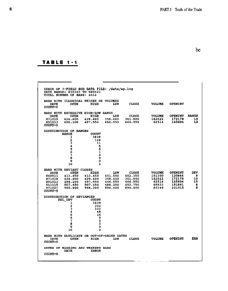
Nonetheless, the presence of such data points should emphasize the fact that market
events involving exceptional ranges do occur and must be managed adequately by a
trading system. All ranges shown in Table l-l are standardized ranges, computed by
dividing a bar’s range by the average range over the last 20 bars. As is common with
market data, the distribution of the standardized range had a longer tail than would
O u t p u t f r o m D a t a - C h e c k i n g U t i l i t y f o r E n d - o f - D a y S & P 5 0 0
C o n t i n u o u s - C o n t r a c t F u t u r e s D a t a f r o m P i n n a c l e
expected given a normally distributed underlying process. Nevertheless, the events of
and
appear to be statistically exceptional: The distribution of all
other range data declined, in an orderly fashion, to zero at a standardized value of 7,
well below the range of 10 seen for the critical bars.
The data-checking utility also flagged 5 bars as having exceptionally deviant
closing prices. As with range, deviance has been defined in terms of a distribution,
using a standardized close-to-close price measure. In this instance,
standard-
ized measure was computed by dividing the absolute value of the difference
between each closing price and its predecessor by
average of the preceding 20
such absolute values.
the 5 flagged (and most deviant) bars were omitted,
the same distributional behavior that characterized the range was observed: a
tailed distribution of close-to-close price change that fell off, in an orderly
ion, to zero at 7 standardized units. Standardized close-to-close deviance scores
of 8 were noted for 3 of the aberrant bars, and scores of 10 were observed
for the remaining 2 bars. Examination of the flagged
points again suggests
that unusual market activity, rather than data error, was responsible for their sta-
tistical deviance. It is not surprising
the 2 most deviant data points were the
same ones noted earlier for their abnormally high range. Finally, the data-check-
ing software did not
any missing bars, bars falling on weekends, or
with
duplicate or out-of-order dates. The only outliers detected appear to be the result
of bizarre market conditions, not
data. Overall, the S&P 500 data series
appears to be squeaky-clean. This was expected: In our experience, Pinnacle Data
Corporation (the source of the data) supplies data of very high quality.
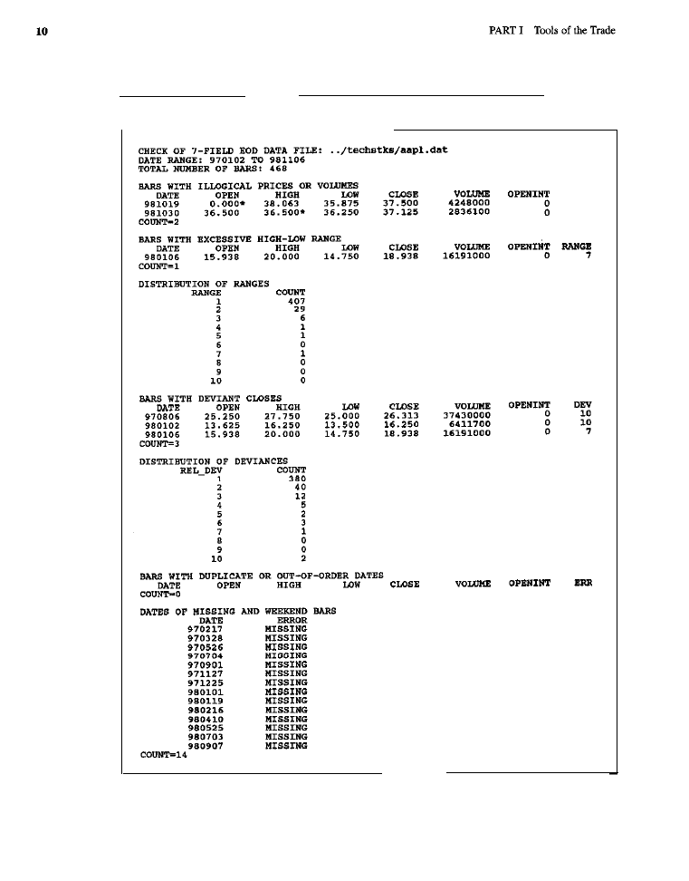
As an example of how bad data quality can get, and the kinds of errors that
can be expected when dealing with low-quality data, another data set was ana-
lyzed with the same data-checking utility. This data, obtained from an acquain-
tance, was for Apple Computer (AAPL). The data-checking results appear in
Table l-2.
In this data set, unlike in the previous one, 2 bars were flagged for having
outright logical inconsistencies. One logically invalid data point had an opening
price of zero, which was also lower than the low, while the other bar had a high
price that was lower than the closing price. Another data point was detected as
having an excessive range, which may or may not be a data error, In addition, sev-
eral bars evidenced extreme closing price deviance, perhaps reflecting uncorrect-
ed stock splits.
were no duplicate or out-of-order dates, but quite a few data
points were missing. In this instance, the missing data points were holidays and,
therefore, only reflect differences in data handling: for a variety of reasons, we
usually fill holidays with data from previous bars. Considering that the data series
extended only from
through 1
(in contrast to the S&P 500, which ran
from
to
it is distressing that several serious errors, including log-
ical violations, were detected by a rather simple scan.
The implication of this exercise is that data should be purchased only from a
T A B L E 1 - 2
Output from Data-Checking Utility for Apple Computer, Symbol AAPL

reputable vendor who takes data quality seriously; this will save time and ensure
reliable, error-free data for system development, testing, and trading, In addition,
all data should be scanned for errors to avoid disturbing surprises. For an in-depth
discussion of data quality, which includes coverage of how data is produced, trans-
mitted, received, and stored, see
(1999).
DATA SOURCES AND VENDORS
Today there are a great
many
from which
data
may be acquired. Data may
be purchased from value-added vendors, downloaded from any of several
exchanges, and extracted from a wide variety of databases accessible over the
Internet and on compact discs.
Value-added vendors, such as Tick Data and Pinnacle, whose data have been
used extensively in this work, can supply the trader with relatively clean data in
easy-to-use form. They also provide convenient update services and, at least in the
case of Pinnacle, error corrections that are handled automatically by the down-
loading software, which makes the task of maintaining a reliable, up-to-date data-
base very straightforward. Popular suppliers of end-of-day commodities data
include Pinnacle Data Corporation
Prophet Financial Systems
Commodities Systems Incorporated (CSI,
and
Technical Tools
historical data, which are needed for
testing short time frame systems, may be purchased from Tick Data
8425) and Genesis Financial Data Services
l-2628). Day traders should
also look into Data Transmission Network (DTN,
Data
Broadcasting Corporation (DBC,
Bonneville Market Information
(BMI,
and
(X00-621 -2628); these data dis-
tributors can provide the fast, real-time data feeds necessary for successful day
trading. For additional information on data sources, consult
(1999). For a
comparative review of end-of-day data, see Knight (1999).
Data need not always be acquired from a commercial vendor. Sometimes it
can be obtained directly from the originator. For instance, various exchanges occa-
sionally furnish data directly to the public. Options data can currently be down-
loaded over the Internet from the Chicago Board of Trade (CBOT). When a new
contract is introduced and the exchange wants to encourage traders, it will often
release a kit containing data and other information of interest. Sometimes this is
the only way to acquire certain kinds of data cheaply and easily.
a vast, mind-boggling array of databases may be accessed using an
Internet web browser or ftp client. These days almost everything is on-line. For exam-
ple, the Federal Reserve maintains files containing all kinds of economic time series
and business cycle indicators. NASA is a great source for solar and astronomical data.
Climate and geophysical data may be downloaded from the National Climatic Data
Center
and the National Geophysical Data Center (NGDC), respectively.

For the ardent net-surfer, there is an
abundance of data in a staggering
variety of formats. Therein, however, lies another problem: A certain level of skill is
required in the art of the search, as is perhaps some basic programming or scripting
experience, as well as the time and effort to find, tidy up, and reformat the data. Since
“time is money,” it is generally best to rely on a reputable, value-added data vendor
for
basic pricing data, and to employ the Internet and other sources for data that is
more specialized or difficult to acquire.
Additional sources of data also include databases available through libraries
and on compact discs.
and other periodical databases offer full text
retrieval capabilities and can frequently be found at the public library. Bring a
floppy disk along and copy any data of interest. Finally, do not forget newspapers
such as
Investor’s Business Daily,
and
Wall
Journal; these can
be excellent sources for certain kinds of information and are available on micro-
film from many libraries.
In general, it is best to maintain data in a standard text-based (ASCII) for-
mat. Such a format has the virtue of being simple, portable across most operating
systems and hardware platforms, and easily read by all types of software, from text
editors to charting packages.

C H A P T E R 2
Simulators
N
savvy trader would trade a system with a real account and risk real money
without first observing its behavior on paper. A trading simulator is a software
application or component that allows the user to simulate, using historical data, a
trading account that is traded with a user-specified set of trading rules. The user’s
trading rules are written into a small program that automates a rigorous
trading” process on a substantial amount of historical data. In this way, the trad-
ing simulator allows the trader to gain insight into how the system might perform
when traded in a real account. The
of a trading simulator is that it
makes it possible to efficiently back-test, or paper-trade, a system to determine
whether the system works and, if so, how well.
TYPES OF SIMULATORS
There are two major forms of trading simulators. One form is the integrated,
to-use software application that provides some basic historical analysis and simu-
lation along with data collection and charting. The other form is the specialized
software component or class library that can be incorporated into user-written
software to provide system testing and evaluation functionality. Software compo-
nents and class libraries offer open architecture, advanced features, and high lev-
els of performance, but require programming expertise and such additional
elements as graphics, report generation, and data management to be useful.
Integrated applications packages, although generally offering less powerful simu-
lation and testing capabilities, are much more accessible to the novice.

PROGRAMMING THE SIMULATOR
Regardless of whether an integrated or component-based simulator is employed,
the trading logic of the user’s system must be programmed into it using some com-
puter language. The language used may be either a generic programming lan-
guage, such as C+ or FORTRAN, or a proprietary scripting language. Without
the aid of a formal language, it would be impossible to express a system’s trading
rules with the precision required for an accurate simulation. The need for pro-
gramming of some kind should not be looked upon as a necessary evil.
Programming can actually benefit the trader by encouraging au explicit and disci-
plined expression of trading ideas.
For an example of how trading logic is programmed into a simulator, consid-
er
a popular integrated product from Omega Research that contains
an interpreter for a basic system writing language (called Easy Language) with
simulation capabilities. Omega’s Easy Language is a proprietary,
specific language based on Pascal (a generic programming language). What does a
simple trading system look like when programmed in Easy Language? The follow-
ing code implements a simple moving-average crossover system:
Simple moving average crossover
in
Easy Language)
parameter
‘A”, contract
(buys at
of next bar)
If
And
at open Of
This system goes long one contract at tomorrow’s open when the close crosses
above its moving average, and goes short one contract when the close crosses
below the moving average. Each order is given a name or identifier: A for the buy:
B for the sell. The length of the moving average (Len) may be set by the user or
optimized by the software.
Below is the same system programmed in
+ using Scientific Consultant
Services’ component-based C-Trader toolkit, which includes the C+ + Trading
Simulator:

Except for syntax and naming conventions, the differences between the
and
Easy Language implementations are small. Most significant are the explicit refer-
ences to the current bar (cb) and to a particular simulated trading account or sim-
ulator class instance (ts) in the C+ implementation. In C+ it is possible to
explicitly declare and reference any number of simulated accounts: this becomes
important
working with portfolios and
(systems that trade the
accounts of other systems), and when developing models that incorporate an
implicit walk-forward adaptation.
SIMULATOR OUTPUT
All good trading simulators generate output containing a wealth of information
about the performance of the user’s simulated account. Expect to obtain data on
gross and net profit, number of winning and losing trades, worst-case
down, and related system characteristics, from even the most basic simulators.
Better simulators provide figures for maximum run-up, average favorable and
adverse excursion, inferential statistics, and more, not to mention highly detailed
analyses of individual trades. An extraordinary simulator might also include in
its output some measure of risk relative to reward, such as the annualized
to-reward ratio (ARRR) or the
Sharp
an important and well-known mea-
sure used to compare the performances of different portfolios, systems, or funds
1994).
The output from a trading simulator is typically presented to the user in the
form of one or more reports. Two basic kinds of reports are available from most trad-
ing simulators: the performance summary and the trade-by-trade, or “detail,” report.
The information contained in these reports can help the trader evaluate a system’s
“trading style” and determine whether the system is
of real-money trading.
Other kinds of reports may also be generated, and the information from the
simulator may be formatted in a way that can easily be run into a spreadsheet for
further analysis. Almost all the tables and charts that appear in this book were pro-
duced in this manner: The output from the simulator was written to a file
would be read by Excel, where the information was further processed and format-
ted for presentation.
Performance Summary Reports
As an illustration of the appearance of performance summary reports, two have
been prepared using the same moving-average crossover system employed to
illustrate simulator programming. Both the
(Table 2-l) and C-Trader
(Table 2-2) implementations of this system were run using their respective target
software applications. In each instance, the length parameter (controls the period
of the moving average) was set to 4.
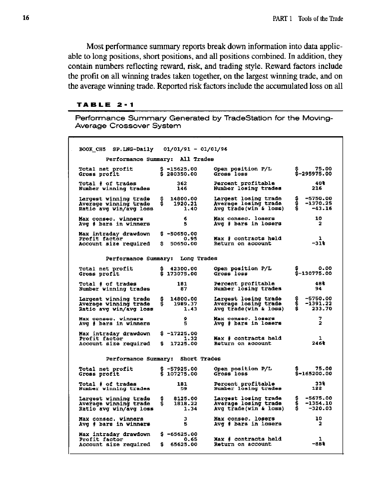

Such style factors as the total number of trades, the number of winning trades, the
number of losing trades, the percentage of profitable trades, the maximum numbers
of consecutive winners and losers, and the average numbers of bars in winners and
losers also appear in performance summary reports. Reward, risk, and style are crit-
ical aspects of system performance that these reports address.
Although all address the issues of reward, risk and trading style, there are a
number of differences between various performance summary reports. Least sig-
nificant are differences in formatting. Some reports, in an effort to cram as much
information as possible into a limited amount of space, round dollar values to the
nearest whole integer, scale up certain values by some factor of 10 to avoid the
need for decimals, and arrange their output in a tabular, spreadsheet-like format.
Other reports use less cryptic descriptors, do not round dollar values or
numbers, and format their output to resemble more traditional reports,
Somewhat more significant than differences in formatting are the variations
between performance summary reports that result from the definitions and
assumptions made in various calculations. For instance, the number of winning
trades may differ slightly between reports because of how winners are defined.
Some simulators count as a winner any trade in which the
P/L
figure
is greater than or equal to zero, whereas others count as winners only trades for
which the
P/L
is strictly greater than zero. This difference in calculation also
affects figures for the average winning trade and for the ratio of the average win-
ner to the average loser. Likewise, the average number of bars in a trade may be
greater or fewer, depending on how they are counted. Some simulators include the
entry bar in all bar counts; others do not. Return-on-account figures may also dif-
fer, depending, for instance, on whether or not they are annualized.
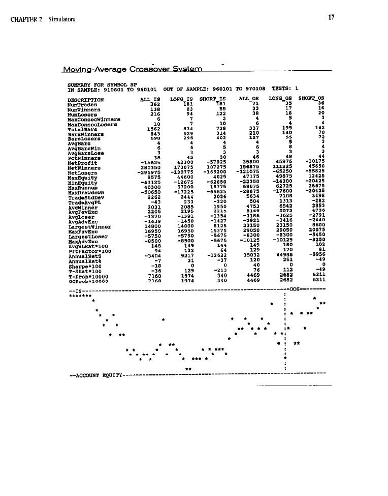
Differences in content between performance summary reports may even be
more significant. Some only break down their performance analyses into long
positions, short positions, and all trades combined. Others break them down into
in-sample and out-of-sample trades, as well. The additional breakdown makes it
easy to see whether a system optimized on one sample of data (the in-sample set)
shows similar behavior on another sample (the out-of-sample data) used for veri-
fication; out-of-sample tests are imperative for optimized systems. Other impor-
tant information, such as the total bar counts, maximum run-up (the converse of
adverse and favorable excursion numbers, peak equity, lowest equity,
annualized return in dollars, trade variability (expressed as a standard deviation),
and the annualized risk-to-reward ratio (a variant of the
Ratio), are present
in some reports. The calculation of inferential statistics, such as the t-statistic and
its associated probability, either for a single test or corrected for multiple tests or
is also a desirable feature. Statistical items, such as t-tests and prob-
abilities, are important since they help reveal whether a system’s performance
reflects the capture of a valid market inefficiency or is merely due to chance or
excessive curve-fitting. Many additional, possibly useful statistics can also be

culated, some of them on the basis of the information present in performance sum-
maries. Among these statistics (Stendahl, 1999) are net positive outliers, net neg-
ative outliers, select net profit (calculated after the removal of outlier trades), loss
ratio (greatest loss divided by net profit),
ratio, longest flat
period, and buy-and-hold return (useful as a baseline). Finally, some reports also
contain a text-based plot of account equity as a function of time.
To the degree that history repeats itself, a clear image of the past seems like
an excellent foundation from which to envision a likely future. A good perfor-
mance summary provides a panoramic view of a trading method’s historical
behavior. Figures on return and risk show how well the system traded on test data
from the historical period under study. The Sharpe Ratio, or annualized risk to
reward, measures return on a risk- or stability-adjusted scale. T-tests and related
statistics may be used to determine whether a system’s performance derives from
some real market inefficiency or is an artifact of chance, multiple tests, or inap-
propriate optimization. Performance due to real market inefficiency may persist
for a time, while that due to artifact is unlikely to recur in the future. In short, a
good performance summary aids in capturing profitable market phenomena likely
to persist; the capture of persistent market inefficiency is, of course, the basis for
any sustained success as a trader.
This wraps up the discussion of one kind of report obtainable within most
trading simulation environments. Next we consider the other type of output that
most simulators provide: the trade-by-trade report.
Trade-by-Trade Reports
Illustrative trade-by-trade reports were prepared using the simulators contained in
(Table 2-3) and in the C-Trader toolkit (Table 2-4). Both reports per-
tain to the same simple moving-average crossover system used in various ways
throughout this discussion. Since hundreds of trades were taken by this system, the
original reports are quite lengthy. Consequently, large blocks of trades have been
edited out and ellipses inserted where the deletions were made. Because these
reports are presented merely for illustration, such deletions were considered
acceptable.
In contrast to a performance report, which provides an overall evaluation of
a trading system’s behavior, a detail or
trade-by-trade
report contains detailed
information on each trade taken in the simulated account. A minimal detail report
contains each trade’s entry and exit dates (and times, if the simulation involves
intraday data), the prices at which these entries and exits occurred, the positions
held (in numbers of contracts, long or short), and the profit or loss resulting from
each trade. A more comprehensive trade-by-trade report might also provide infor-
mation on the type of order responsible for each entry or exit (e.g., stop, limit, or
market), where in the bar the order was executed (at the open, the close, or in
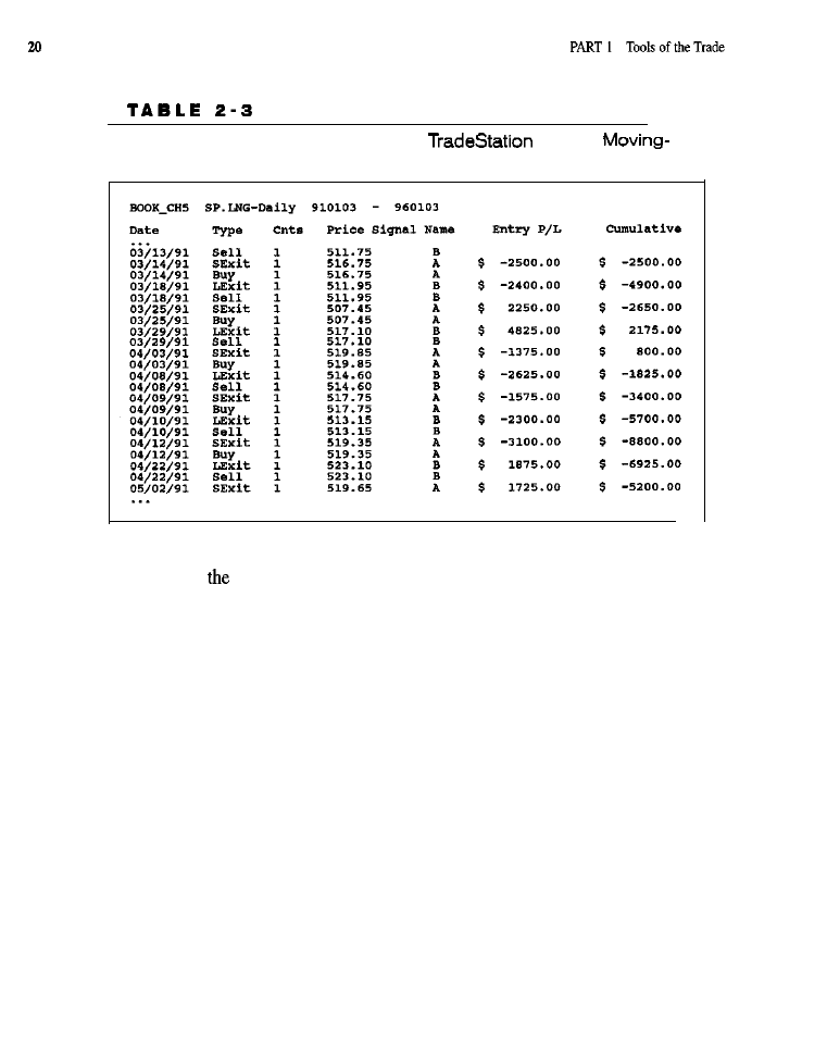
Trade-by-Trade Report Generated by
for the
Average Crossover System
between),
number of bars each
trade
was held, the account equity at the start
of each trade, the maximum favorable
and
adverse excursions within each trade,
and the account equity on exit from each trade.
Most trade-by-trade reports contain the
date
(and time, if applicable) each
trade was entered, whether a buy or sell was involved (that is, a long or short posi-
tion established), the number of contracts in the transaction, the date the trade
was exited, the profit or loss on the trade, and the cumulative profit or loss on all
trades up to and including the trade under consideration. Reports also provide the
name of the order on which the trade was entered and the name of the exit order.
A better trade-by-trade report might include the fields for
maximum favorable
excursion (the greatest unrealized profit to occur during each trade), the maxi-
mum
adverse
excursion (the largest unrealized loss), and the number of bars each
trade was held.
As with the performance summaries, there are differences between various
trade-by-trade reports with respect to the ways they are formatted and in the
assumptions underlying the computations on which they are based.
While the performance summary provides a picture of the whole forest, a good
trade-by-trade report focuses on the trees. In a good trade-by-trade report, each trade
is scrutinized in detail: What was the worst paper loss sustained in this trade? What
would the profit have been with a perfect exit? What was the actual profit (or loss)
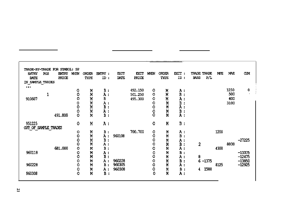
T A B L E
2 - 4
Trade-by-Trade Report Generated Using the C-Trader Toolkit for the Moving-Average Crossover System
910527
- 1
492.150
910528
492.150
-1
501.250
910613 1
495.300
910614 -1
492.200
910618
1 496.900
910620 -1
. . .
1
691.500
960101
- 1
692.600
960104
1
700.700
960108
- 1
691.600
960110
1 697.600
960111 -1
1 663.000
9 6 0 2 1 6
-1 729.300
960223 1
727.500
-1
724.750
960305
1 722.900
-1
725.900
:
910528
910607
910613
910614
910618
910620
910625
492.200
496.900
491.800
490.650
960101
692.600
960104
691.600
960110
697.600
960111
661.000
960118
683.000
960216
729.300
960223
727.500
724.750
722.900
725.900
960311
716.150
2 0
11
4 5 5 0
7 2975
2 -1550
5 -2350
3 -2550
6 575
8 550
4 -4050
5 -4550
3 -3000
-8300
8 -1000
30 23150
900
7 925
4 4875
500
6900
4025
0
525
400
1650
4550
1525
5975
2825
3625
2550
1075
500
1650
1725
325 -15625
1675
1450
0
29050
8400
5725
4475
4075
4050
-19675
5100 -24225
3000
-35525
2325 -36525
1450
1875
2750
2525
1275
1300
-11425
-6550

on the trade? Has the trading been fairly consistent? Are recent trades worse than
those of the past? Or are they better? How might some of the worst trades be char-
acterized in a way to improve the trading system? These are the kinds of questions
that
be answered by a distant panoramic view of the forest (a summary
report), but they can be answered with a good trade-by-trade or detail report. In addi-
tion, a properly formatted detail report can be loaded into a spreadsheet for further
analysis. Spreadsheets are convenient for sorting and displaying data. They make it
easy, for instance, to draw histograms. Histograms can be very useful in decisions
regarding the placement of stops (Sweeney, 1993). Histograms can show how much
of the potential
in the trades is being captured by the system’s exit strategy and
is also helpful in designing profit targets. Finally, a detailed examination of the worst
and best trades may generate ideas for improving the system under study.
SIMULATOR PERFORMANCE
Trading simulators vary dramatically in such aspects of performance as speed,
capacity, and power. Speed is important when there is a need to carry out many
tests or perform complex optimizations, genetic or otherwise. It is also essential
when developing systems on complete portfolios or using long, intraday data
series involving thousands of trades and hundreds of thousands of data points. In
some instances, speed may determine whether certain explorations can even be
attempted. Some problems are simply not practical to study unless the analyses
can be accomplished in a reasonable length of time. Simulator capacity involves
problem size restrictions regarding the number of bars on which a simulation may
be performed and the quantity of system code the simulator can handle. Finally,
the power a simulator gives the user to express and test complex trading ideas, and
to run tests and even system optimizations on complete portfolios, can be signifi-
cant to the serious, professional trader. A fairly powerful simulator is required, for
example, to run many of
trading models examined in this book.
Speed
The most significant determinant of simulation processing speed is the nature of
the scripting or programming language used by the simulator, that is, whether
the language is compiled or interpreted. Modern optimizing compilers for gener-
ic languages, such as
FORTRAN, and Pascal/Delphi, translate the
written source code into highly efficient machine code that the processor can
execute directly at full bore; this makes simulator toolkits that use such lan-
guages and compilers remarkably fast. On the other hand, proprietary, interpret-
ed languages, such as Microsoft’s Visual Basic for Applications and Omega’s
Easy Language, must be translated and fed to the processor line by line.
Simulators that employ interpreted languages can be quite sluggish, especially
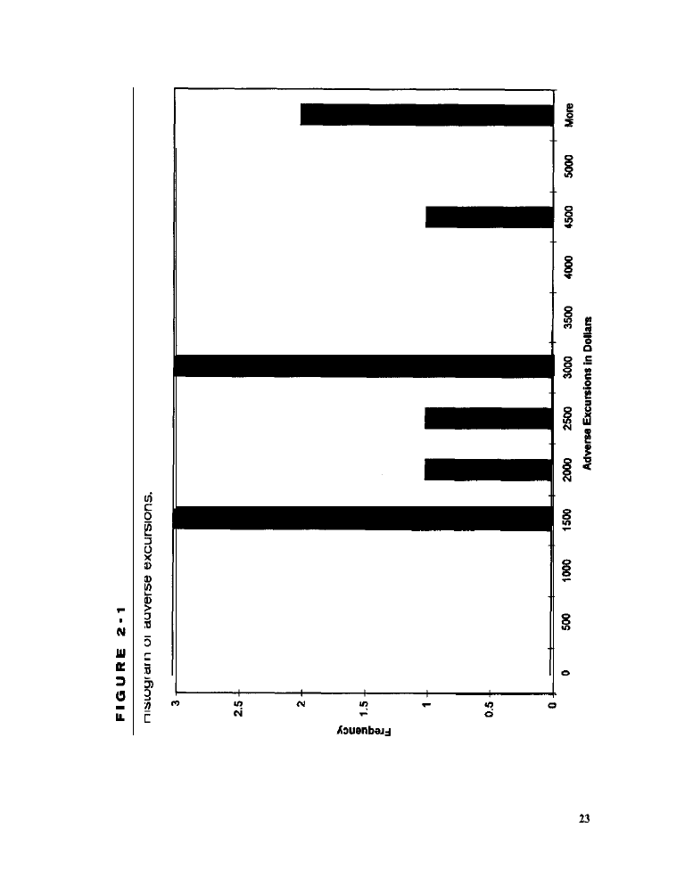
when executing complex or “loopy” source code. Just how much speed can be
gained using a compiled language over an interpreted one? We have heard
claims of systems running about 50 times faster since they were converted from
proprietary languages to C+ + !
Capacity
While speed is primarily a function of language handling (interpreted versus com-
piled), capacity is mostly determined by whether 16-bit or 32-bit software is used.
Older, 16-bit software is often subject to the dreaded 64K limit. In practical terms,
this means that only about 15,000 bars of data (about 4 days of ticks, or 7 weeks of
l-minute bars on the S&P 500) can be loaded for system testing. In addition, as the
system code is embellished, expect to receive a message to the effect that the sys-
tem is too large to verify. Modem C+ + or FORTRAN products, on the other hand,
work with standard
C+ + or FORTRAN compilers. Consequently, they have
a much greater problem size capacity: With continuous-contract data on a machine
with sufficient memory, every single tick of the S&P 500 since its inception in 1983
can easily be loaded and studied! In addition, there are virtually no limits on the
number of trades a system can take, or on the system’s size and complexity. All
modern
FORTRAN, and Pascal/Delphi compilers are now full
pro-
grams that generate code for, and run under, 32-bit operating systems, such as
Windows 95, Windows NT, or
Any simulator that works with such
a compiler should be able to handle large problems and enormous data sets with
ease. Since most software packages are upgrading to 32-bit status, the issue of
problem size capacity is rapidly becoming less significant than it once was.
Differences in simulator power are attributable mostly to language and to design.
Consider language first: In this case, it is not whether the language is compiled or
interpreted, as was the case for speed, but rather its expressive power. Can the most
elaborate and unusual trading ideas be expressed with precision and grace? In
some languages they can; in others they cannot. It is unfortunate that the most
powerful languages have steep learning curves. However, if one can climb the
curve, a language like
+ makes it possible to do almost anything imaginable.
Your word processor, spreadsheet, web browser, and even operating system were
all probably written in C++ or its predecessor, C. Languages like C++ and
Object Pascal (the basis of Borland’s Delphi) are also extensible and can easily be
customized for the purpose of trading system development by the use of appro-
priate libraries and add-on components. Visual Basic and Easy Language,
although not as powerful as general-purpose, object-oriented languages like
or Object Pascal, have gentler learning curves and are still quite capable as

guages go. Much less powerful, and not really adequate for the advanced system
developer, are the macro-like languages embedded in popular charting packages,
e.g.,
International’s
The rule of thumb is the more powerful the
language, the more powerful the simulator.
Design issues are also a consideration in a simulator’s power. Extendability
and modularity are especially important. Simulators that employ C+ + or Object
Pascal (Borland’s Delphi) as their native language are incredibly extensible and
can be highly modular, because such general-purpose, object-oriented languages
are themselves highly extensible and modular; they were designed to be so from
the ground up. Class libraries permit the definition of
data types and opera-
tors. Components can provide encapsulated functionality, such as charting and
database management. Even old-fashioned function libraries (like the Numerical
Algorithms Group library, the International Mathematics and Statistics Library
and
Numerical Recipes library) are available to satisfy a variety of needs. Easy
Language, too, is highly extensible and modular: Modules called User Functions
can be created in
Language, and
written in other languages
(including
C+
can be called (if they are placed in a dynamic link library, or
DLL). Macrolike languages, on the other hand, are not as flexible, greatly limit-
ing their usefulness to the advanced system developer. In our view, the ability to
access modules written in other languages is absolutely crucial: Different lan-
guages have different expressive foci, and even with a powerful language like
C+
it sometimes makes sense to write one or more modules in another
guage such as Prolog (a language designed for writing expert systems).
One additional design issue, unrelated to the language employed, is relevant
when discussing simulator power: whether a simulator can work with whole portfo-
lios as well as with individual
Many products are not designed to perform
simulations and optimizations on whole portfolios at once, although sometimes
ons are available that make it possible to generate portfolio performance analyses
after the fact. On the other hand, an appropriately designed simulator can make mul-
tiple-account or portfolio simulations and system
straightforward.
RELIABILITY OF SIMULATORS
Trading simulators vary in their reliability and trustworthiness. No complex soft-
ware, and that includes trading simulation software, is completely bug-free. This
is true even for reputable vendors with great products. Other problems pertain to
the assumptions made regarding ambiguous situations in which any of several
orders could be executed in any of several sequences during a bar. Some of these
items, e.g., the so-called bouncing tick (Ruggiero,
can make it seem like the
best system ever had been discovered when, in fact, it could bankrupt any trader.
It seems better that a simulator makes worst-case assumptions in ambiguous situ-
ations: this way, when
trading begins, there is greater likelihood of having

a pleasant, rather than an unpleasant, surprise. All of this boils down to the fact
that when choosing a simulator, select one that has been carefully debugged, that
has a proven track record of reliability, and in which the assumptions and handling
of ambiguous situations are explicitly stated. In addition, learn the simulator’s
quirks and how to work around them.
CHOOSING THE RIGHT SIMULATOR
If you are serious about developing sophisticated trading systems, need to work
with large portfolios, or wish to perform tests using individual contracts or
options, then buckle down, climb the learning curve, and go for an advanced sim-
ulator that employs a generic programming language such as the C++ or Object
Pascal. Such a simulator will have an open architecture that provides access to an
incredible selection of add-ons and libraries: technical analysis libraries, such as
those from PM Labs
and Scientific Consultant Services
3333); and general numerical algorithm libraries, such as Numerical Recipes
Numerical Algorithms Group (NAG)
and
International Mathematics and Statistics Library (IMSL), which cover statistics,
linear algebra, spectral analysis, differential equations, and other mathematics.
Even neural network and genetic algorithm libraries are readily available.
Advanced simulators that employ generic programming languages also open up a
world of third-party components and graphical controls which cover everything
from sophisticated charting and data display to advanced database management,
and which are compatible with Borland’s C++ Builder and Delphi, as well as
with Microsoft’s Visual Basic and Visual C+
If your needs are somewhat less stringent, choose a complete, integrated solu-
tion Make sure the simulation language permits procedures residing in
to be
called when necessary. Be wary of products that are primarily charting tools with
limited programming capabilities if your intention is to develop, back-test, and trade
mechanical systems that go significantly beyond traditional or “canned” indicators.
SIMULATORS USED IN THIS BOOK
We personally prefer simulators built using modern, object-oriented programming
practices. One reason for our choice is that an object-oriented simulator makes it
easy to create as many simulation instances or simulated accounts as might be
desired. This is especially useful when simulating the behavior of a trading system
on an entire portfolio of
(as is done in most tests in this book), rather than
on a single instrument. An object-oriented simulator also comes in handy when
building adaptive, self-optimizing systems where it is sometimes necessary to
implement internal simulations. In addition, such software makes the construction
of
(systems that trade in or out of the equity curves of other systems)

a simple matter. Asset allocation models, for instance, may be treated as
terns that dynamically allocate capital to individual trading systems or accounts. A
good object-oriented simulator can generate the portfolio equity curves and other
information needed to create and back-test asset allocation models operating on
top of multiple trading systems. For these reasons, and such others as familiarity,
most tests carried out in this book have been performed using the C-Trader toolk-
it. Do not be alarmed. It is not necessary to have any expertise in C+ + or mod-
em software practices to benefit from this book. The logic of every system or
system element examined will be explained in great detail in the text.

C H A P T E R 3
Optimizers and Optimization
t would be nice to develop trading systems without giving a thought to opti-
mization. Realistically, however,
development of a profitable trading strategy
is a trial-and-error activity in which some form of optimization always plays a
role. There is always an optimizer around somewhere-if not visible on the table,
lurking in the shadows.
An
is simply an entity or algorithm that attempts to find the best
possible solution to a problem;
optimization
is the search process by which
solution is discovered. An optimizer may be a self-contained software component,
perhaps implemented as a C++ class, Delphi object, or
control.
Powerful, sophisticated optimizers often take
form of software components
designed to be integrated into user-written programs. Less sophisticated opti-
mizers, such as those found in high-end simulation and charting packages, are usu-
ally simple algorithms implemented with a few lines of programming code. Since
any entity or algorithm that performs optimization is an optimizer, optimizers need
not be associated with computers or machines at all; an optimizer may be a per-
son engaged in problem-solving activities. The human brain is one of the most
powerful heuristic optimizers on earth!
WHAT OPTIMIZERS DO
Optimizers exist to find the best possible solution to a problem. What is meant by
the
best possible
solution to a
problem?
Before attempting to define that phrase,
let us first consider what constitutes a solution. In trading, a solution is a
lar set of trading rules and perhaps system parameters,

All trading systems have at least two mles (an entry rule and an exit rule), and
most have one or more parameters.
Rules express
the logic of the trading system,
and generally appear as “if-then” clauses in whatever language the trading system has
been written. Parameters determine the behavior of the logic expressed in the rules;
they can include lengths of moving averages, connection weights in neural networks,
thresholds used in comparisons, values that determine placements for stops and prof-
it targets, and other similar items.
simple moving-average crossover system,
used in the previous chapter to illustrate various trading simulators, had two rules:
one for the buy order and one for the sell order. It also had a single parameter, the
length of the moving average. Rules and parameters completely define a trading sys-
tem and determine its performance. To obtain the best performance from a trading
system, parameters may need to be adjusted and rules juggled.
There is no doubt that some rule and parameter combinations
systems
that trade well, just as others specify systems that trade poorly; i.e., solutions dif-
fer in their quality. The goodness of a solution or trading model, in terms of how
well it performs when measured against some. standard, is often
The
converse of fitness, the inadequacy of a solution, is frequently referred to as
In practice, fitness is evaluated by
function,
a block of programming
code that calculates a single number that reflects the relative desirability of any
solution. A fitness function can be written to appraise fitness howsoever the trader
desires. For example, fitness might be interpreted as net profit penalized for exces-
sive drawdown. A
works in exactly the same way, but higher numbers
signify worse solutions. The sum of the squared errors, commonly computed when
working with linear regression or neural network models, is a cost function.
The best possible solution a problem
can now be defined: It is that partic-
ular solution that has the greatest fitness or the least cost. Optimizers endeavor to
find the best possible solution to a problem by maximizing fitness, as measured by
a
function, or minimizing cost, as computed by a cost function.
The best possible solution to a problem may be discovered in any number of
ways. Sometimes problems can be solved by simple trial-and-error, especially when
guided by human insight into the problem being worked. Alternatively, sophisticated
procedures and algorithms may be necessary. For example, simulating the process of
evolution (as genetic optimizers do) is a very powerful way to discover or evolve
high-quality solutions to complex problems. In some cases, the best problem solver
is an analytic (calculus-based) procedure, such as a conjugate gradient. Analytic opti-
mization is an efficient approach for problems with smooth (differentiable) fitness
surfaces, such those encountered in training neural networks, developing multiple
linear regression models, or computing simple-structure factor rotations.
HOW OPTIMIZERS ARE USED
Optimizers are wonderful tools that can be used in a myriad of ways. They help
shape the aircraft we fly, design the cars we drive, and even select delivery routes

3
Optimizers and Optimization
31
for our mail. Traders sometimes use optimizers to discover rule combinations that
trade profitably. In Part II, we will demonstrate how a genetic optimizer can evolve
profitable rule-based entry models. More commonly, traders call upon optimizers
to determine the most appropriate values for system parameters; almost any kind
of optimizer, except perhaps an analytic optimizer, may be employed for this pur-
pose. Various kinds of optimizers, including powerful genetic algorithms, are
effective for training or evolving neural or fuzzy logic networks. Asset allocation
problems yield to appropriate optimization strategies. Sometimes it seems as if the
only limit on how optimizers may be employed is the user’s imagination, and
therein lies a danger: It is easy to be seduced into “optimizer abuse” by the great
and alluring power of this tool. The correct and incorrect applications of opti-
mizers are discussed later in this chapter.
TYPES OF OPTIMIZERS
There are many kinds of optimizers, each with its own special strengths and weak
advantages and disadvantages. Optimizers can be classified along such
dimensions as human versus machine, complex versus simple, special purpose
versus general purpose, and analytic versus stochastic. All optimizers-regardless
of kind, efficiency, or reliability-execute a search for the best of many potential
solutions to a formally specified problem.
Optimizers
A mouse cannot be used to click on a button that says “optimize.” There is no spe-
cial command to enter. In fact, there is no special software or even machine in
sight. Does this mean there is no optimizer? No. Even when there is no optimizer
apparent, and it seems as though no optimization is going on, there is. It is known
as implicit optimization and works as follows: The
tests a set of rules based
upon some ideas regarding the market. Performance of the system is poor, and so
the trader reworks the ideas, modifies the system’s rules, and runs another simu-
lation Better performance is observed. The trader repeats this process a few
times, each time making changes based on what has been learned along the way.
Eventually, the trader builds a system worthy of being traded with real money.
Was this system an optimized one? Since no parameters were ever explicitly
adjusted and no rules were ever rearranged by the software, it appears as if the
trader has succeeded in creating an unoptimized system. However, more than one
solution from a set of many possible solutions was tested and the best solution was
selected for use in trading further study. This means that the system was opti-
mized after all! Any form of problem solving in which more than one solution is
examined and the best is chosen constitutes de facto optimization. The trader has
a powerful brain that employed mental problem-solving algorithms, e.g., heuris-
tically guided trial-and-error ones, which are exceptionally potent optimizers.
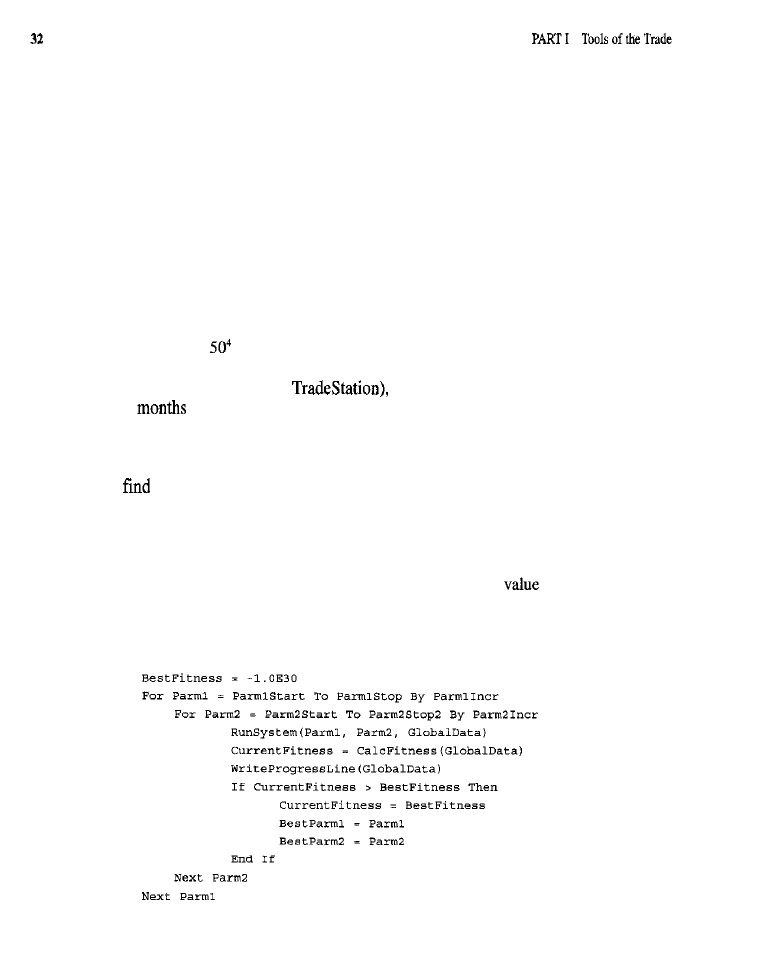
This means that optimization is always present: optimizers are always at work.
There is no escape!
Brute Force Optimizers
A
brute
force
optimizer
searches for the best possible solution by systematically
testing all potential solutions, i.e., all definable combinations of rules, parameters,
or both. Because every possible combination must be tested, brute force opti-
mization can be very slow. Lack of speed becomes a serious issue as the number
of combinations to be examined grows. Consequently, brute force optimization is
subject to the law of “combinatorial explosion.” Just how slow is brute force opti-
mization? Consider a case where there are four parameters to optimize and where
each parameter can take on any of 50 values. Brute force optimization would
require
that
(about
6 million) tests or simulations be conducted before the
optimal parameter set could be determined: if one simulation was executed every
1.62 seconds (typical for
the optimization process would take about
4
to complete. This approach is not very practical, especially when many
systems need to be tested and optimized, when there are many parameters, when
the parameters can take on many values, or when you have a life. Nevertheless,
brute force optimization is useful and effective. If properly done, it will always
the best possible solution. Brute force is a good choice for small problems
where combinatorial explosion is not an issue and solutions can be found in min-
utes, rather than days or years.
Only a small amount of programming
code
is needed to implement
brute
force optimization. Simple loop constructs are commonly employed. Parameters
to be optimized are stepped from a start value to a stop
by
some increment
using a For loop (C, C+ +, Basic, Pascal/Delphi) or a Do loop (FORTRAN). A
brute force optimizer for two parameters, when coded in a modem dialect of
Basic, might appear as follows:

Because brute force optimizers are conceptually simple and easy to program,
they are often built into the more advanced software packages that arc available
for traders.
As a practical illustration of bmte force optimization,
was used
to optimize the moving averages in a dual moving-average crossover system.
Optimization was for net profit, the only trading system characteristic
Station can optimize without the aid of add-on products, The Easy Language code
for the dual moving-average trading model appears below:
The system was optimized by stepping the length of the first moving average
from 2 to 10 in increments of 2. The length of the second moving average
was advanced from 2 to 50 with the same increments. Increments were set
greater than 1 so that fewer than
combinations would need to be tested
can only save data on a maximum of 200 optimization runs). Since
not all possible combinations of values for the two parameters were explored, the
optimization was less thorough than it could have been; the best solution may have
been missed in the search. Notwithstanding, the optimization required 125 tests,
which took 3 minutes and 24 seconds to complete on 5 years of historical, end-of-
day data, using an Intel 486 machine running at 66 megahertz. The results gener-
ated by the optimization were loaded into an Excel spreadsheet and sorted for net
profit. Table 3-l presents various performance measures for the top 25 solutions.
In the table, LENA represents the period of the shorter moving average,
the period of the longer moving average,
the total net profit,
the net profit for long positions,
the net profit for short posi-
tions,
the profit factor, ROA the total (unannualized) return-on-account,
the maximum drawdown,
the total number of trades taken, and
the percentage of profitable trades.
Since optimization is a problem-solving search procedure, it frequently
results in surprising discoveries. The optimization performed on the dual moving-
average crossover system was no exception to the
Conventional trading wis-
dom says that “the trend is your friend.” However, having a second moving average
that is faster than the first, the most profitable solutions in Table I trade against
the trend. These profitable countertrend solutions might not have been discovered
without the search performed by the optimization procedure.
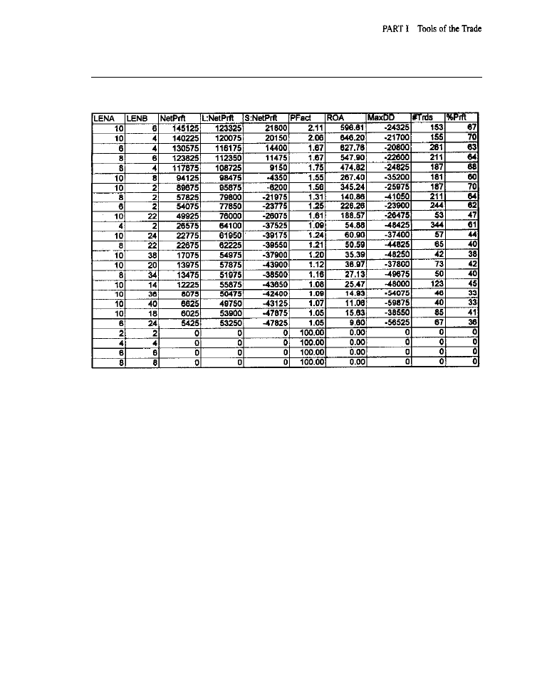
3 4
T A B L E

Successful user-guided optimization calls for skill, domain knowledge, or
both, on
part of the person guiding the optimization process. Given adequate
skill and experience, not to mention a tractable problem, user-guided optimization
can be extremely efficient and dramatically faster than brute force methods.
speed and efficiency derive from the addition of intelligence to the search process:
Zones with a high probability of paying off can be recognized and carefully exam-
ined, while time-consuming investigations of regions unlikely to yield good
results can be avoided.
User-guided optimization is most appropriate when ballpark results have
already been established by other means, when the problem is familiar or well
understood, when only a small number of parameters need to be manipulated.
As a means of “polishing” an existing solution, user guided-optimization is an
excellent choice. It is also useful for studying model sensitivity to changes in rules
or parameter values.
Genetic Optimizers
Imagine something powerful enough to solve all the problems inherent in the
creation of a human being. That something surely represents the ultimate in
problem solving and optimization. What is it? It is the familiar process of evo-
lution. Genetic
endeavor to harness some of that incredible prob-
lem-solving power through a crude simulation of the evolutionary process. In
terms of overall performance and the variety of problems that may be solved,
there is no general-purpose optimizer more powerful than a properly crafted
genetic one.
Genetic optimizers are
optimizers in the sense that they take
advantage of random chance in their operation. It may not seem believable that
tossing dice can be a great way to solve problems, but, done correctly, it can be!
In addition to randomness, genetic optimizers employ selection and recombina-
tion. The clever integration of random chance, selection, and recombination is
responsible for the genetic optimizer’s great power. A full discussion of genetic
algorithms, which are the basis for genetic optimizers, appears in Part II.
Genetic optimizers have many highly desirable characteristics. One such
characteristic is speed, especially when faced with combinatorial explosion. A
genetic optimizer can easily be many orders of magnitude faster than a brute force
optimizer when there are a multiplicity of rules, or parameters that have many pos-
sible values, to manipulate. This is
because,
like user-guided optimization, genetic
optimization can focus on important regions of solution space while mostly ignor-
ing blind alleys. In contrast to user-guided optimization, the benefit of a selective
search is achieved without the need for human intervention.
Genetic optimizers can swiftly solve complex problems, and they are also
more immune than other kinds of optimizers to the effects of local maxima in the

fitness surface or, equivalently, local minima in the cost surface. Analytic methods
are worst in that they almost always walk right to the top of the nearest hill or bot-
tom of the nearest valley, without regard to whether higher hills or lower valleys
exist elsewhere. contrast, a good genetic optimizer often locates the globally
best solution-quite an impressive feat when accomplished for cantankerous fit-
ness surfaces, such as those associated with matrices of neural connection weights.
Another characteristic of genetic optimization is that it works well with fit-
ness surfaces marked by discontinuities, flat regions, and other troublesome irreg-
ularities. Genetic optimization shares this characteristic with brute force,
user-guided, annealing-based, and other nonanalytic optimization methods.
Solutions that maximize such items as net profit, return on investment, the Sharpe
Ratio, and others that define difficult, nonanalytic fitness landscapes can be found
using a genetic optimizer. Genetic optimizers shine with difficult fitness functions
that lie beyond the purview of analytic methods. This does not mean that they can-
not be used to solve problems having more tractable fitness surfaces: Perhaps
slower than the analytic methods, they have the virtue of being more resistant to
the traps set by local optima.
Overall, genetic optimizers are the optimizers of choice when there are many
parameters or rules to adapt, when a global solution is desired, or when arbitrarily
complex (and not necessarily differentiable or continuous) fitness or cost functions
must be handled. Although special-purpose optimizers can outperform genetic opti-
mizers on specific kinds of problems, for general-purpose optimization, genetic
optimizers are among the most powerful tools available.
What does a genetic optimizer look like in action? The dual moving-average
crossover system discussed earlier was translated to Cl 1 so that the genetic opti-
mizer in the C-Trader toolkit could be used to solve for the two system parame-
ters,
and
the period of the first moving average, was examined
over the range of 2 through 50, as was
the period of the second moving aver-
age. Optimization was for net profit so that the results would be directly compa-
rable with those produced earlier by brute force optimization. Below is the Cl 1
code for the crossover system:

3
Optimizers and
no
in
910302) (
0.0; continue; )
To solve for the best parameters, brute force optimization would require that 2,041
tests be performed; in
that works out to about 56 minutes of com-
puting time, extrapolating from the earlier illustration in which a small subset of
the current solution space was examined. Only 1 minute of running time was
required by the genetic optimizer; in an attempt to put it at a significant disadvan-
tage, it was prematurely stopped after performing only 133 tests.
The output from the genetic optimizer appears in Table 3-2. In this table,
PI
rep-
resents the period of the faster moving average,
P2 the
period of the slower moving
average,
total net profit, NETLNG the net profit for long positions,
the net profit for short positions,
PFAC the
factor,
the annualized
on account,
DRAW
the maximum drawdown,
TRDS
the number of trades taken by the
system,
WIN%
the percentage of winning trades,
AVGT
the profit or loss resulting
from the average trade, and
fitness of the solution (which, in this instance, is
merely the total net
As with the brute force data in Table 3-1, the genetic data
have been sorted by net profit (fitness) and only the 25 best solutions were presented.
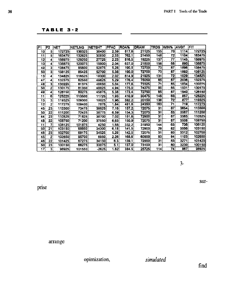
Top 25 Solutions Found Using Genetic Optimization in C-Trader Toolkit
Comparison of the brute force and genetic optimization results (Tables 1 and 3-2,
respectively) reveals that the genetic optimizer isolated a solution with a greater net
profit ($172,725) than did the brute force optimizer ($145,125). This is no surprise
since a larger solution space, not decimated by increments, was explored. The
is that the better solution was found so quickly, despite the handicap of a pre-
maturely stopped evolutionary process. Results like these demonstrate the incredible
effectiveness of genetic optimization.
Optimization by Simulated Annealing
Optimizers based on annealing mimic the thermodynamic process by which liq-
uids freeze and metals anneal. Starting out at a high temperature, the atoms of a
liquid or molten metal bounce rapidly about in a random fashion. Slowly cooled,
they
themselves into an orderly configuration-a crystal-that represents
a minimal energy state for the system. Simulated in software, this thermodynamic
process readily solves large-scale optimization problems.
As with genetic
optimization by
annealing is a very
powerful Stochastic technique, modeled upon a natural phenomenon, that can
globally optimal solutions and handle ill-behaved fitness functions. Simulated
annealing has effectively solved significant combinatorial problems, including

3
Optimizers and Optimization
the famous “traveling salesman problem,” and the problem of how best to arrange the
millions of circuit elements found on modem integrated circuit chips, such as
those that power computers. Methods based on simulated annealing should not be
construed as limited to combinatorial optimization; they can readily be adapted to
the optimization of real-valued parameters. Consequently, optimizers based on
simulated annealing are applicable to a wide variety of problems, including those
faced by traders.
Since genetic optimizers perform so well, we have experienced little need to
explore optimizers based on simulated annealing. In addition, there have been a
few reports suggesting that, in many cases, annealing algorithms do not perform
as well as genetic algorithms. Because of these reasons, we have not provided
examples of simulated annealing and have little more to say about the method.
Analytic Optimizers
Analysis
(as in “real analysis” or “complex analysis”) is an extension of classical
college calculus.
Analytic optimizers
involve the well-developed machinery of
analysis, specifically differential calculus and the study of analytic functions, in
the solution of practical problems.
some instances, analytic methods can yield
a direct (noniterative) solution to an optimization problem. This happens to be the
case for multiple regression, where solutions can be obtained with a few matrix
calculations. In multiple regression, the goal is to find a set of regression weights
that minimize the sum of the squared prediction errors. In other cases, iterative
techniques must be used. The connection weights in a neural network, for exam-
ple, cannot be directly determined. They must be estimated using an iterative pro-
cedure, such as back-propagation.
Many iterative techniques used to solve multivariate optimization prob-
lems (those involving several variables or parameters) employ some variation
on
the theme of
steepest ascent.
In its most basic form, optimization by steep-
est ascent works as follows: A point in the domain of the fitness function (that
is, a set of parameter values) is chosen by some means. The gradient vector at
that point is evaluated by computing the derivatives of the fitness function with
respect to each of the variables or parameters; this defines the direction in
dimensional parameter space for which a fixed amount of movement will pro-
duce the greatest increase in fitness. A small step is taken up the hill in fitness
space, along the direction of the gradient. The gradient is then recomputed at
this new point, and another, perhaps smaller, step is taken. The process is
repeated until convergence occurs.
A real-world implementation of steepest ascent optimization has to specify
how the step size will be determined at each iteration, and how the direction
defined by the gradient will be adjusted for better overall convergence of the opti-
mization process. Naive implementations assume that there is an analytic fitness

surface (one that can be approximated locally by a convergent power series) hav-
ing hills that must be climbed. More sophisticated implementations go further,
commonly assuming that the fitness function can be well approximated locally by
a quadratic form. If a fitness function satisfies this assumption, then much faster
convergence to a solution can be achieved. However, when the fitness surface has
many irregularly shaped bills and valleys, quadratic forms often fail to provide a
good approximation. In such cases, the more sophisticated methods break down
entirely or their performance seriously degrades.
Worse than degraded performance is the problem of local solutions. Almost
all analytic methods, whether elementary or sophisticated, are easily trapped by
local maxima: they generally fail to locate the globally best solution when there
many hills and valleys in the fitness surface. Least-squares, neural network
predictive modeling gives rise to fitness surfaces that, although clearly analytic,
are full of bumps, troughs, and other irregularities that lead standard analytic tech-
niques (including back-propagation, a variant on steepest ascent) astray. Local
maxima and other hazards that accompany such fitness surfaces can, however, be
sidestepped by cleverly marrying a genetic algorithm with an analytic one. For tit-
surfaces amenable to analytic optimization, such a combined algorithm can
provide the best of both worlds: fast, accurate solutions that are also likely to be
globally optimal.
Some fitness surfaces are simply not amenable to analytic optimization.
More specifically, analytic methods cannot be used when the fitness surface has
flat areas or discontinuities in the region of parameter space where a solution is to
be sought. Flat areas imply null gradients, hence the absence of a preferred direc-
tion in which to take a step. At points of discontinuity, the gradient is not defined;
again, a stepping direction cannot be determined. Even if a method does not
explicitly use gradient information, such information is employed implicitly by
the optimization algorithm. Unfortunately, many fitness functions of interest to
traders-including, for instance, all functions that involve net profit, drawdown,
percentage of winning trades, risk-to-reward ratios, and other like items-have
plateaus and discontinuities. They are, therefore, not tractable using analytic methods.
Although the discussion has centered on the maximization of fitness, every-
thing said applies as well to the minimization of cost. Any maximization technique
can be used for minimization, and vice versa: Multiply a fitness function by 1 to
obtain an equivalent cost function; multiply a cost function by 1 and a fitness func-
tion is the result. If a minimization algorithm takes your fancy, but a maximization
is required, use this trick to avoid having to recode the optimization algorithm.
Linear Programming
The techniques of linear programming are designed for optimization problems
involving linear cost or fitness functions, and linear constraints on the parameters

or input variables. Linear programming is typically used to solve resource allo-
cation problems. In the world of trading, one use of linear programming might be
to allocate capital among a set of investments to maximize net profit. If
adjusted profit is to be optimized, linear programming methods cannot be used:
Risk-adjusted profit is not a linear function of the amount of capital allocated to
each of the investments; in such instances, other techniques (e.g., genetic algo-
rithms) must be employed. Linear programming methods are rarely useful in the
development of trading systems. They are mentioned here only to inform readers
of their existence.
HOW TO FAIL WITH OPTIMIZATION
Most traders do not seek failure, at least not consciously. However, knowledge of
the way failure is achieved can be of great benefit when seeking to avoid it. Failure
with an optimizer is easy to accomplish by following a few key rules. First, be sure
to use a small data sample when running
The smaller the sample, the
greater the likelihood it will poorly represent the data on which the trading model
will actually be traded. Next, make sure the trading system has a large number of
parameters and rules to optimize: For a given data sample, the greater the number
of variables that must be estimated, the easier it will be to obtain spurious results.
It would also be beneficial to employ only a single sample on which to run tests;
annoying out-of-sample data sets have no place in the rose-colored world of the
ardent loser. Finally, do avoid the headache of inferential statistics. Follow these
rules and failure is guaranteed.
What shape will failure take? Most likely, system performance will look
great in tests, but terrible in real-time trading. Neural network developers call this
phenomenon “poor generalization”; traders are acquainted with it through the
experience of margin calls and a serious loss of trading capital. One consequence
of such a failure-laden outcome is the formation of a popular misconception: that
all optimization is dangerous and to be feared.
In actual fact, optimizers are not dangerous and not all optimization should be
feared. Only bad optimization is dangerous and frightening. Optimization of large
parameter sets on small samples, without out-of-sample tests or inferential statis-
tics, is simply a bad practice that invites unhappy results for a variety of reasons.
Small Samples
Consider the impact of small samples on the optimization process. Small samples
of market data are unlikely to be representative of the universe from which they
are drawn: consequently, they will probably differ significantly from other sam-
ples obtained from the same universe. Applied to a small development sample, an
optimizer will faithfully discover the best possible solution. The best solution for

the development sample, however, may turn out to be a dreadful solution for the
later sample on which genuine trades will be taken. Failure ensues, not because
optimization has found a bad solution, but because it has found a good solution to
the wrong problem!
Optimization on inadequate samples is also good at spawning solutions that
represent only mathematical artifact. As the number of data points declines to the
number of free (adjustable) parameters, most models (trading, regression, or other-
wise) will attain a perfect tit to even random data. The principle involved is the
same
one responsible for the fact that a line, which is a two-parameter model, can
always
be
drawn through any two distinct points, but cannot always be
made to
intersect three arbitrary points. In statistics, this is known as the
degrees-of-freedom
issue; there are as many degrees of freedom as there are data points beyond that
which can be fitted perfectly for purely mathematical reasons. Even when there are
enough data points to avoid a totally artifact-determined solution, some part of the
model fitness obtained through optimization will be of an artifact-determined
nature, a by-product of the process.
For multiple regression models, a formula is available that can be used to
estimate how much “shrinkage” would occur in the multiple correlation coeffi-
cient (a measure of model fitness) if the artifact-determined component were
removed. The
shrinkage
correction
formula,
which shows the relationship
between the number of parameters (regression coefficients) being optimized, sam-
ple size, and decreased levels of apparent fitness (correlation) in tests on new sam-
ples, is shown below in FORTRAN-style notation:
In this equation, represents the number of data points, the number of model
parameters,
R
multiple correlation coefficient determined for the sample by the
regression (optimization) procedure, and
RC
the shrinkage-corrected multiple cor-
relation coefficient. The inverse formula, one that estimates the
inflated correlation
given the true correlation
existing in the population
from which the data were sampled, appears below:
These formulas, although legitimate only for linear regression, are not bad
for estimating how well a fully trained neural network model-which is nothing
more than a particular kind of
regression-will generalize. When work-
ing with neural networks, let represent the total number of connection weights
in the model. In addition, make sure that simple correlations are used when work-
ing with these formulas; if a neural network or regression package reports the
squared multiple correlation, take the square root.

4 3
Large Parameter Sets
An excessive number of free parameters or rules will impact an optimization effort
in a manner similar to an
number of data points. As the number of ele-
ments undergoing optimization rises, a model’s ability to capitalize on idiosyn-
crasies in the development sample increases along with the proportion of the
model’s fitness that can be attributed to mathematical artifact. The result of opti-
mizing a large number of variables-whether rules, parameters, or both-will be
a model that performs well on the development data, but poorly on out-of-sample
test data and in actual trading.
It is not the absolute number of free parameters that should be of concern,
but the number of parameters relative to the number of data points. The shrinkage
formula discussed in the context of small samples is also heuristically relevant
here: It illustrates how the relationship between the number of data points and the
number of parameters affects the outcome. When there are too many parameters,
given the number of data points, mathematical artifacts and capitalization on
chance (curve-fitting, in the bad sense) become reasons for failure.
No
One of the better ways to get into trouble is by failing to verify model performance
using out-of-sample tests or inferential statistics. Without such tests, the spurious
solutions resulting from small samples and large parameter
not to mention
other less obvious causes, will go undetected. The trading system that appears to
be ideal on the development sample will be put “on-line,” and devastating losses
will follow. Developing systems without subjecting them to out-of-sample and sta-
tistical tests is like flying blind, without a safety belt, in an uninspected aircraft.
HOW TO SUCCEED WITH OPTIMIZATION
Four steps can be taken to avoid failure and increase the odds of achieving suc-
cessful optimization. As a first step, optimize on the largest possible representative
sample and make sure many simulated trades are available for analysis. The sec-
ond step is to keep the number of free parameters or rules small, especially in rela-
tion to sample size. A third step involves running tests on out-of-sample data, that
is, data not used or even seen during the optimization process. As a fourth and
step, it may be worthwhile to statistically assess the results.
Large, Representative Samples
As suggested earlier, failure is often a consequence of presenting an optimizer with
the wrong problem to solve. Conversely, success is likely when the optimizer is

presented with the right problem. The conclusion is that trading models should be
optimized on data from the near future,
data that will actually be traded; do that
and watch the profits roll in. The catch is where to find tomorrow’s data today.
Since the future has not yet happened, it is impossible to present the opti-
mizer with precisely the problem that
needs
to be solved. Consequently, it is nec-
essary to attempt the next-best alternative: to present
optimizer with a broader
problem, the solution to which should be as applicable as possible to the actual,
but impossible-to-solve, problem. One way to accomplish this is with a data sam-
ple that, even though not drawn from the future, embodies many characteristics
that might appear in future samples. Such a
data
sample should include bull
and
bear markets, trending and nontrending periods, and even crashes. In addition, the
data in the sample should be as recent as possible so that it will reflect current pat-
terns of market behavior. This is what is meant by a representative sample.
As well as representative, the sample should be large. Large samples make it
harder for optimizers to uncover spurious or artifact-determined solutions.
Shrinkage,
the expected decline in performance on unoptimized data, is reduced
when large samples are employed in the optimization process.
Sometimes, however, a trade-off must be made between the sample’s size
and the extent to which it is representative. As one goes farther back in history to
bolster a sample, the data may become less representative of current market con-
ditions. In some instances,
is a clear transition point beyond which the data
become much less representative: For example, the S&P 500 futures began trad-
ing in 1983, effecting a structural change in the general market. Trade-offs become
much less of an issue when working with intraday data on short time frames,
where tens of thousands or even hundreds of thousands of bars of data can
be
gath-
ered without
going
back beyond the recent past.
Finally, when running simulations and
pay attention to the
number of trades a system takes. Like large data samples, it is highly desirable that
simulations and tests involve numerous trades. Chance or artifact can easily be
responsible for any profits produced by a system that takes only a few trades,
regardless of the number of data points used in the test!
Few Rules and Parameters
To achieve success, limit the number of free rules and parameters, especially when
working with small data samples. For a given sample size, the fewer the rules or
parameters to optimize, the greater the likelihood that a trading system will main-
tain its performance in out-of-sample tests
and
real-time trading. Although sever-
al dozen parameters may be acceptable when working with several thousand
trades taken on 100,000 l-minute bars (about year for the S&P 500 futures),
even two or three parameters may be excessive when developing a system using a
few years of end-of-day data. If a particular model requires many parameters, then

significant effort should be put into assembling a mammoth sample (the legendary
Gann supposedly went back over 1,000 years in his study of wheat prices). An
alternative that sometimes works is optimizing a trading model on a whole port-
folio, using the same rules and parameters across all markets-a technique used
extensively in this book.
Verification of Results
After optimizing the rules and parameters of a trading system to obtain good
behavior on the development or in-sample data, but before risking any real money,
it is essential to verify the system’s performance in some manner. Verification of
system performance is important because it gives the trader a chance to veto
and embrace success: Systems that fail the test of verification can be discard-
ed, ones that pass can be traded with confidence. Verification is the single most
critical step on the road to success with optimization or, in fact, with any other
method of discovering a trading model that really works.
To ensure success, verify any trading solution using out-of-sample tests or
inferential statistics, preferably both. Discard any solution that fails to be profitable
in an out-of-sample test: It is likely to fail again when the rubber hits the road.
Compute inferential statistics on all tests, both in-sample and out-of-sample. These
statistics reveal the probability that the performance observed in a sample reflects
something real that will hold
in other samples and in real-time trading. Inferential
statistics work by making probability inferences based on the distribution of
itability in a system’s trades or returns. Be
to use statistics that are corrected for
multiple tests when analyzing in-sample optimization results. Out-of-sample tests
should be analyzed with standard, uncorrected statistics. Such statistics appear in
some of the
reports that are displayed in the chapter on simulators. The
use of statistics to evaluate trading systems is covered in depth in the following chap-
ter. Develop a working knowledge of statistics; it will make you a better trader.
Some suggest checking a model for sensitivity to small changes in parame-
ter values. A model highly tolerant of such changes is more “robust” than a model
not as tolerant, it is said. Do not pay too much attention to these claims. In truth,
parameter tolerance cannot be relied upon as a gauge of model robustness. Many
extremely robust models are highly sensitive to the values of certain parameters.
The only true arbiters of system robustness are statistical and, especially,
sample tests.
ALTERNATIVES TO TRADITIONAL OPTIMIZATION
There are two major alternatives to traditional optimization: walk-forward opti-
mization and self-adaptive systems. Both of these techniques have the advantage
that any tests carried out are, from start to finish, effectively out-of-sample.
Examine the performance data, run some inferential statistics, plot the equity
curve, and the system is ready to be traded. Everything is clean and mathemati-
cally unimpeachable. Corrections for shrinkage or multiple tests, worries over
excessive curve-fitting, and many of the other concerns that plague traditional
optimization methodologies can be forgotten. Moreover, with today’s modem
computer technology, walk-forward and self-adaptive models are practical and not
even difficult to implement.
The principle behind
walk-forward optimization
(also known as
walk-for-
ward testing) is to emulate the steps involved in actually trading a system that
requires periodic optimization. It works like this: Optimize the system on the data
points
1
through
M.
Then simulate trading on data points
+ I through
M +
Reoptimize the system on data points + 1 through +
M.
Then simulate trad-
ing on points
1 through (K
+
Advance through
the data series
in this fashion until no more data points are left to analyze. As should be evident,
the system is optimized on a sample of historical data and then traded. After some
period of time, the system is reoptimized and trading is resumed. The sequence of
events guarantees that the data on which trades take place is always in the future
relative to the optimization process; all trades occur on what is, essentially,
sample data. In walk-forward testing,
M
is the look-back or optimization window
and
the reoptimization interval.
Self-adaptive
systems work in a similar manner, except that the optimization
or adaptive process is part of the system, rather than the test environment. As each
bar or data point
comes
along, a self-adaptive system updates its internal state (its
parameters or rules) and then makes decisions concerning actions required on the
next bar or data point. When the next
bar
arrives, the decided-upon actions are car-
ried out and the process repeats. Internal updates, which are how the system learns
about or adapts to the market, need not occur on every single bar. They can be per-
formed at fixed intervals or whenever deemed necessary by the model.
The trader planning to work with self-adapting systems will need a power-
ful, component-based development platform that employs a strong language, such
as
Object Pascal, or Visual Basic, and that provides
good
access to
party libraries and software components. Components are designed to
be
incorpo-
rated into user-written software, including the special-purpose software that
constitutes an adaptive system. The more components that are available, the less
work there is to do. At the very least, a trader venturing into self-adaptive systems
should have at hand genetic optimizer and trading simulator components that can
be easily embedded within a trading model. Adaptive systems will be demonstrat-
ed in later chapters, showing how this technique works in practice.
There is no doubt that walk-forward optimization and adaptive systems will
become more popular over time as the markets become more efficient and diffi-
cult to trade, and as commercial software packages become available that place
these techniques within reach of the average trader.

3 optimizers and
OPTIMIZER TOOLS AND INFORMATION
Aerodynamics, electronics, chemistry, biochemistry, planning, and business are
just a few of the
in which optimization plays a role. Because optimization is
of interest to so many problem-solving areas, research goes on everywhere, infor-
mation is abundant, and optimization tools proliferate. Where can this information
be found? What tools and products are available?
force optimizers are usually buried in software packages aimed
at tasks other than optimization; they are usually not available on
own.
In the world of trading, products like
and
from Omega
Research
from Futures Truth
and
from Equis International (800-882-3040) have built-in brute force opti-
mizers. If you write your own software, brute force optimization is so trivial to
implement using in-line progranuning code that the use of special libraries or
components is superfluous. Products and code able to carry out brute force opti-
mization may also serve well for user-guided optimization.
Although sometimes appearing as built-in tools in specialized programs,
genetic optimizers are
often distributed in the form of class libraries or soft-
ware components, add-ons to various application packages, or stand-alone research
instruments. As an example of a class library written with the component paradigm
in mind, consider
the C+ genetic optimizer from Scientific Consultant
Services (516-696-3333): This general-purpose genetic optimizer implements sev-
eral algorithms, including differential
evolution,
and is sold in the form of highly
portable C+ + code that can be used in
DOS, and Windows envi-
ronments. TS-Evolve, available from
Associates (800-21 l-9785) gives
users of
the ability to perform full-blown genetic
The
which can be purchased from Palisade Corporation
is a
general-purpose genetic optimizer for Microsoft’s Excel spreadsheet; it comes with
a dynamic link library (DLL) that can provide genetic optimization services to user
programs written in any language able to call DLL functions. GENESIS, a stand-
alone instrument aimed at the research community, was written by John
of the Naval Research Laboratory; the product is available in the form of generic C
source
code.
While genetic optimizers can occasionally be found in modeling tools
for chemists and in other specialized products, they do not yet form a native part of
popular software packages designed for traders.
Information about genetic optimization is readily available. Genetic algo-
rithms are discussed in many
books,
magazines, and journals and on Internet
newsgroups. A good overview of the field of genetic optimization can be found in
the
Handbook
of Generic Algorithms (Davis, 1991). Price and Storm (1997)
described an algorithm for “differential evolution,” which has been shown to be an
exceptionally powerful technique for optimization problems involving real-valued
parameters. Genetic algorithms are currently the focus of many academic journals
and conference proceedings. Lively discussions on all aspects of genetic opti-
mization take place in several Internet newsgroups of which
is the
most noteworthy.
A basic exposition of simulated annealing can be found in
Recipes in C (Press et al.,
as can C functions implementing optimizers for
both combinatorial and real-valued problems. Neural, Novel Hybrid Algorithms
for
Time Series Prediction (Masters, 1995) also discusses annealing-based opti-
mization and contains relevant C+ + code on the included CD-ROM. Like genet-
ic optimization, simulated annealing is the focus of many research studies,
conference presentations, journal articles, and Internet newsgroup discussions.
Algorithms and code for conjugate gradient and variable metric optimiza-
tion, two fairly sophisticated analytic methods, can be found in Numerical Recipes
in C (Press et al., 1992) and Numerical Recipes (Press et al., 1986). Masters (1995)
provides an assortment of analytic optimization procedures in C+ + (on the
ROM that comes with his book), as well as a good discussion of the subject.
Additional procedures for analytic optimization are available in the
and the
NAG library (from Visual Numerics, Inc., and Numerical Algorithms Group,
respectively) and in the optimization toolbox for
(a general-purpose
mathematical package from The
that has gamed pop-
ularity in the financial engineering community). Finally, Microsoft’s Excel spread-
sheet contains a built-in analytic optimizer-the Solver-that employs conjugate
gradient or Newtonian methods.
As a source of general information about optimization applied to trading sys-
tem development, consult Design, Testing and Optimization
Trading Systems by
Robert
(1992). Among other things, this book shows the reader how to opti-
mize profitably, how to avoid undesirable curve-fitting, and how to carry out
forward tests.
WHICH OPTIMIZER IS FOR YOU?
At the very least, you should have available an optimizer
is designed to make
both brute force and user-guided optimization easy to carry out. Such an optimiz-
er is already at hand if you use either
or
for system devel-
opment tasks. On the other hand, if you develop your systems in Excel, Visual
Basic, C+
or Delphi, you will have to create your own brute force optimizer.
As demonstrated earlier, a brute force optimizer is simple to implement. For many
problems, brute force or user-guided optimization is the best approach.
If your system development efforts require something beyond brute force, a
genetic optimizer is a great second choice. Armed with both brute force and genet-
ic optimizers, you will be able to solve virtually any problem imaginable. In our
own efforts, we hardly ever reach for any other kind of optimization tool!
users will probably want TS-Evolve from Ruggiero Associates. The

product from Palisade Corporation is a good choice for Excel and Visual
Basic users. If you develop systems in C+ or Delphi, select the C+ + Genetic
Optimizer from Scientific Consultant Services, Inc. A genetic optimizer is the
Swiss Army knife of the optimizer world: Even problems more efficiently solved
using such other techniques as analytic optimization will yield, albeit
slowly,
to a good genetic optimizer.
Finally, if you want to explore analytic optimization or simulated annealing,
we suggest Numerical
Recipes
in C (Press et al., 1992) and Masters (1995) as
good sources of both information and code. Excel users can try out the built-in
Solver tool.

C H A P T E R 4
Statistics
any trading system developers have little familiarity with inferential statistics.
This is a rather perplexing state of affairs since statistics are essential to assessing
the behavior of trading systems. How, for example, can one judge whether an
apparent edge in the trades produced by a system is real or an artifact of sampling
or chance? Think of it-the next sample may not merely be another test, but an
actual trading exercise. If the system’s “edge” was due to chance, trading capital
could quickly be depleted. Consider optimization: Has the system been tweaked
into great profitability, or has the developer only succeeded in the nasty art of
curve-fitting? We have encountered many system developers who refuse to use
any optimization strategy whatsoever because of their irrational fear of curve-fit-
ting, not knowing that the right statistics can help detect such phenomena. In short,
inferential statistics can help a trader evaluate the likelihood that a system is cap-
turing a real inefficiency and will perform as profitably in the future as it has in
the past. In this book, we have presented the results of statistical analyses when-
ever doing so seemed useful and appropriate.
Among the kinds of inferential statistics that are most useful to traders are
t-tests, correlational statistics, and such nonparametric statistics as the runs test.
are useful for determining the probability that the mean or sum of any
series of independent values (derived from a sampling process) is greater or less
than some other such mean, is a fixed number, or falls within a certain band. For
example, t-tests can reveal the probability that the total profits from a series of
trades, each with its individual
figure, could be greater than some thresh-
old as a result of chance or sampling. These tests are also useful for evaluating
of returns, e.g., the daily or monthly returns of a portfolio over a period of
years. Finally, t-tests can help to set the boundaries of likely future performance
51

(assuming no structural change in the market), making possible such statements as
“the probability that the average profit will be between and in the future is
greater than
Correlational
help determine the degree of relationship between
different variables. When applied inferentially, they may also be used to assess
whether any relationships found are “statistically significant,” and not merely due
to chance. Such statistics aid in setting confidence intervals or boundaries on the
“true” (population) correlation, given the observed correlation for a specific sam-
ple.
statistics are essential when searching for predictive variables to
include in a neural network or regression-based trading model.
Correlational statistics, as well as such
statistics as the
test,
are useful in assessing serial dependence or serial correlation. For instance, do prof-
itable trades come in streaks or runs that are then followed by periods of unprofitable
trading? The runs test can help determine whether this is actually occurring. If there
is serial dependence in a system, it is useful to know it because the system can then
be revised to make use of the serial dependence. For example, if a system has clear
ly defined streaks of winning and losing, a metasystem can be developed. The
system would take every trade after a winning trade until the
losing trade comes
along, then stop trading until a
trade is hit, at which point it would again
begin taking trades. If there really are runs, this strategy, or something similar, could
greatly improve a system’s behavior.
WHY USE STATISTICS TO EVALUATE TRADING
SYSTEMS?
It is very important to determine whether any observed profits are real (not
facts of testing), and what the likelihood is that the system producing them will
continue to yield profits in the future when it is used in actual trading. While
of-sample testing can provide some indication of whether a system will hold up on
new (future) data, statistical methods can provide additional information and esti-
mates of probability. Statistics can help determine whether a system’s perfor-
mance is due to chance alone or if the trading model has some real validity.
Statistical calculations can even be adjusted for a known degree of curve-fitting,
thereby providing estimates of whether a chance pattern, present in the data sam-
ple being used to develop the system, has been curve-fitted or whether a pattern
present in the population (and hence one that would probably be present in future
samples drawn from the market being examined) has been modeled.
It should be noted that statistics generally make certain theoretical assumptions
about the data samples and populations to which they may be appropriately applied.
These assumptions are often violated when dealing with trading models. Some vio-
lations have little practical effect and may be ignored, while others may be worked
around. By using additional statistics, the more serious violations can sometimes be

detected, avoided, or compensated for; at the very least, they can be understood. In
short, we are fully aware of these violations and will discuss our acts of hubris and
their ramifications after a foundation for understanding the issues has been laid.
SAMPLING
Fundamental to statistics and, therefore, important to understand, is the act of
sampling, which is the extraction of a number of data points or trades (a sample)
from a larger, abstractly defined set of data points or trades (a
The
central idea behind statistical analysis is the use of samples to make inferences
about the populations from which they are drawn. When dealing with trading
models, the populations will most often be defined as all raw data (past, present,
and future) for a given tradable (e.g., all
bars on all futures on the S&P
all trades (past, present, and future) taken by a specified system on a given
tradable, or all yearly, monthly, or even daily returns. All quarterly earnings
(past, present, and future) of IBM is another example of a population. A sample
could be the specific historical data used in developing or testing a system, the
simulated trades taken, or monthly returns generated by the system on that data.
When creating a trading system,
developer usually draws a sample of
data from the population being modeled. For example, to develop an S&P 500 sys-
tem based on the hypothesis “If yesterday’s close is greater than the close three
days ago, then the market will rise tomorrow,” the developer draws a sample of
end-of-day price data from the S&P 500 that extends back, e.g., 5 years. The hope
is that the data sample drawn from the S&P 500 is
of that market,
i.e., will accurately reflect the actual, typical behavior of that market (the popula-
tion from which the sample was drawn), so that the system being developed will
perform as well in the future (on a previously unseen sample of population data)
as it did in the past (on the sample used as development data). To help determine
whether the system will hold up, developers sometimes test systems on one or
more
periods, i.e., on additional samples of data that have not been
used to develop or optimize the trading model. In our example, the S&P 500 devel-
oper might use 5 years of
1991 through
develop and tweak
the system, and reserve the data from 1996 as the out-of-sample period on which
to test the system. Reserving one or more sets of out-of-sample data is strongly
recommended.
One problem with drawing data samples from financial populations arises
from the complex and variable nature of the markets: today’s market may not be
tomorrow’s Sometimes the variations are very noticeable and their causes are
easily discerned, e.g., when the S&P 500 changed in 1983 as a result of the intro-
duction of futures and options. In such instances, the change may be construed as
having created two distinct populations: the S&P 500 prior to 1983 and the S&P
500 after 1983. A sample drawn from the earlier period would almost certainly

not be representative of the population defined by the later period because it was
drawn from a different population! This is, of course, an extreme case. More
often, structural market variations
due to subtle influences that are sometimes
impossible to identify, especially before the fact. In some cases, the market may
still be fundamentally the same, but it may be going through different phases;
each sample drawn might inadvertently be taken from a different phase and be
representative of that phase alone, not of the market as a whole. How can it be
determined that the population from which a sample is drawn for the purpose of
system development is the same as the population on which the system will be
traded? Short of hopping into a time machine and sampling the future, there is no
reliable way to tell if tomorrow will be the day the market undergoes a
killing metamorphosis! Multiple out-of-sample tests, conducted over a long peri-
od of time, may provide some assurance that a system will hold up, since they
may show that the market has not changed substantially across several sampling
periods. Given a representative sample, statistics can help make accurate infer-
ences about the population from which the sample was drawn. Statistics cannot,
however, reveal whether tomorrow’s market will have changed in some funda-
mental manner.
OPTIMIZATION AND CURVE-FITTING
Another issue found in trading system development is optimization, i.e., improv-
ing the performance of a system by adjusting its parameters until the system per-
forms its best on what the developer hopes is a representative sample. When the
system fails to hold up in the future (or on out-of-sample data), the optimization
process is pejoratively called curve-fitting. However, there is good curve-fitting
and bad curve-fitting. Good curve-fitting is when a model can be fit to the entire
relevant population (or, at least, to a sufficiently large sample thereof), suggesting
that valid characteristics of the entire population have been captured in the model.
Bad
occurs when the system only fits chance characteristics, those
that are not necessarily representative of the population from which the sample
was drawn.
Developers are correct to fear bad curve-fitting, i.e., the situation in which
parameter values are adapted to the particular sample on which the system was
optimized, not to the population as a whole. If the sample was small or was not
representative of the population from which it was drawn, it is likely that the sys-
tem will look good on that one sample but fail miserably on another, or worse, lose
money in real-time trading. However, as the sample gets larger, the chance of this
happening becomes smaller: Bad curve-fitting declines and good curve-fitting
increases. All the statistics discussed reflect this, even the ones that specifically
concern optimization. It is true that the more combinations of things optimized,
the greater the likelihood good performance may be obtained by chance alone.

However, if the statistical result was sufficiently good, or the sample on which it
was based large enough to reduce the probability that the outcome was due to
chance, the result might still
be very
real and significant, even if many parameters
were optimized.
Some have argued that size does not matter, i.e., that sample size and the
number of trades studied have little or nothing to do with the risk of
and that a large sample does not mitigate curve-fitting. This is patently
untrue, both intuitively and mathematically. Anyone would have less confidence in
a system that took only three or four trades over a lo-year period than in one that
took over 1,000 reasonably profitable trades. Think of a linear regression model in
which a straight line is being fit to a number of points. If there are only two points,
it is easy to fit the line perfectly every time, regardless of where the points
located. If there are three points, it is harder. If there is a scatterplot of points, it is
going to be harder still, unless those points reveal some real characteristic of
population that involves a linear relationship.
The linear regression example demonstrates that bad curve-fitting does
become more difficult as the sample size gets larger. Consider two trading sys-
tems: One system had a profit per trade of $100, it took 2 trades, and the stan-
dard deviation was $100 per trade: the other system took 1,000 trades, with
similar means and
deviations. When evaluated statistically, the system
with 1,000 trades will be a lot more “statistically significant” than the one with
the 2 trades.
In multiple linear regression models, as the number of regression parameters
(beta weights) being estimated is increased relative to the sample size, the amount
of curve-fitting increases and statistical significance lessens for the same
degree of model fit. In other words, the greater the degree of curve-fitting, the
harder it is to get statistical significance. The exception is if the improvement in fit
when adding regressors is sufficient to compensate for the loss in significance due
to the additional parameters being estimated. In fact, an estimate of
shrinkage
(the
degree to which the multiple correlation can be expected to shrink when computed
using out-of-sample
data) can
even be calculated given sample size and number of
regressors: Shrinkage increases with regressors and decreases with sample size. In
short, there is mathematical evidence that curve-fitting to chance characteristics of
a sample, with concomitant poor generalization, is more likely if the sample is
small relative to the number of parameters being fit by the model. In fact, as (the
sample size) goes to infinity, the probability that the curve-fitting (achieved by
optimizing a set of parameters) is nonrepresentative of the population goes to zero.
The larger the number of parameters being optimized, the larger the sample
required. In the language of statistics, the parameters being estimated use up the
available “degrees of freedom.”
All this leads to the conclusion that the larger the sample, the more likely its
“curves” are representative of characteristics of the market as a whole. A small

sample almost certainly will be nonrepresentative of the market: It is unlikely that
its curves will reflect
of the entire market that persist over time. Any model
built using a small sample will be capitalizing purely on the chance of sampling.
Whether curve-fitting is “good” or “bad” depends on if it was done to chance or
to real market patterns, which, in turn, largely depends on
size and
tiveness of the sample. Statistics are useful because they make it possible to take
curve-fitting into account when evaluating a system.
When dealing with neural networks, concerns about overtraining or general-
ization are tantamount to concerns about bad curve-fitting. If the sample is large
enough and representative, curve-fitting some real characteristic of the market is
more likely, which may be good because the model should fit the market. On the
other hand, if the sample is small, the model will almost certainly be fit to pecu-
liar characteristics of the sample and not to the behavior of the market generally.
In neural networks, the concern about whether the neural network will generalize
is the same as the concern about whether other kinds of systems will hold up in
future. To a great extent, generalization depends on
size of the sample on
which the neural network is trained. The larger the sample, or the smaller the num-
ber of connection weights (parameters) being estimated, the more likely the net-
work will generalize. Again, this can be demonstrated mathematically by
examining simple cases.
As was the case with regression, au estimate of shrinkage (the opposite of
generalization) may be computed when developing neural networks. In a very real
sense, a neural network is actually a multiple regression, albeit, nonlinear, and the
correlation of a neural net’s output with the target may be construed as a multiple
correlation coefficient. The multiple correlation obtained between a net’s output
and the target may be corrected for shrinkage to obtain some idea of how the net
might perform on out-of-sample data. Such shrinkage-corrected multiple correla-
tions should routinely be computed as a means of determining whether a network
has merely curve-fit the data or has discovered something useful. The formula for
correcting a multiple correlation for shrinkage is as follows:
A FORTRAN-style expression was used for reasons of typsetting. In this for-
mula,
represents the square root operator; N is the number of data points
or, in the case of neural networks, facts; P is the number of regression
or, in the case of neural networks, connection weights; R represents the
uncorrected multiple correlation; and RC is the multiple correlation corrected
for shrinkage. Although this formula is strictly applicable only to linear multi-
ple regression (for which it was originally developed), it works well with neur-
al networks and may be used to estimate how much performance was inflated on
in-sample
data
due to curve-fitting. The formula expresses a relationship
between sample size, number of parameters, and deterioration of results. The

statistical correction embodied in the shrinkage formula is used in the chapter on
network entry models.
SAMPLE SIZE AND
Although, for statistical reasons, the system developer should seek the largest
ple possible, there is a trade-off between sample size and representativeness when
dealing with the financial markets. Larger samples mean samples that go
back in time, which is a problem because the market of years ago may be funda-
mentally different from the market of today-remember the S&P 500 in
This means that a larger sample may sometimes be a less representative sample,
or one that confounds several distinct populations of data! Therefore, keep in mind
that, although the goal is to have the largest sample possible, it is equally impor-
tant to try to make sure the period from which the sample is drawn is still repre-
sentative of the market being predicted.
EVALUATING A SYSTEM STATISTICALLY
Now that some of the basics are out of the way, let us look at how statistics are
used when developing and evaluating a trading system. The examples below
employ a system that was optimized on one sample of data (the m-sample data)
and then run (tested) on another sample of data (the out-of-sample data). The
of-sample evaluation of this system will be discussed before the in-sample one
because the statistical analysis was simpler for the former (which is equivalent to
the evaluation of an unoptimized trading system) in that no corrections for mul-
tiple tests or optimization were required. The system is a lunar model that trades
the S&P 500; it was published in an article we wrote (see Katz with McCormick,
June 1997). The
code for this system is shown below:

Example 1: Evaluating the Out-of-Sample Test
Evaluating an optimized system on a set of out-of-sample data that was never used
during the optimization process is identical to evaluating an unoptimized system.
In both cases, one test is run without adjusting any parameters. Table 4-1 illus-
trates the use of statistics to evaluate an unoptimized system: It contains the
of-sample or verification results together with a variety of statistics. Remember, in
this test, a fresh set of data was used; this data was not used as the basis for
adjustments in the system’s parameters.
The parameters of the trading model have already been set. A sample of data
was drawn from a period in
past, in this specific case,
through
this is the out-of-sample or verification data. The model was then run on this
of-sample data, and it generated simulated trades. Forty-seven trades were taken.
This set of trades can itself be considered a sample of trades, one drawn from the
population of all trades that the system took in the past or will take in the future;
i.e., it is a sample of trades taken from the universe or population of all trades for
that system. At this point, some inference must be made regarding the average
profit per trade in the population as a whole, based on the sample of trades. Could
the performance obtained in the sample be due to chance alone? To find the
answer, the system must be statistically evaluated.
To begin statistically evaluating this system, the sample mean (average) for
(the number of trades or
size) must first be calculated. The mean is
simply the sum of the profit/loss figures for the trades generated divided by (in
this
case, 47).
The sample
mean was $974.47
per trade. The
standard deviation
(the variability in the trade profit/loss figures) is then computed by subtracting
the sample mean from each of the
for all 47 trades in the
sample; this results in 47 (n) deviations. Each of the deviations is then squared,
and then all squared deviations are added together. The sum of the squared devi-
ations is divided hy I (in this case, 46). By taking the square root of the
resultant number (the
mean squared deviation),
the
sample standard deviation
is
obtained. Using the sample standard deviation, the expected
standard deviation
of
the
is computed: The sample standard deviation (in this case,
is divided by the square root of the sample size. For this example, the expected
standard deviation of the mean was $888.48.
To determine the likelihood that the observed profitability is due to chance
alone, a simple
is calculated. Since the sample profitability is being compared
with no profitability, zero is subtracted from the sample mean trade profit/loss (com-
puted earlier).
resultant number is then divided by the sample standard devia-
tion to obtain the value of the t-statistic, which in this case worked out to be 1.0968.
Finally the probability of getting such a large t-statistic by chance alone (under the
assumption that the system was not profitable in the population from which the sam-
ple was drawn) is calculated:
The cumulative t-distribution
for that t-statistic is
with the appropriate degrees of freedom, which in
case was
1, or 46.
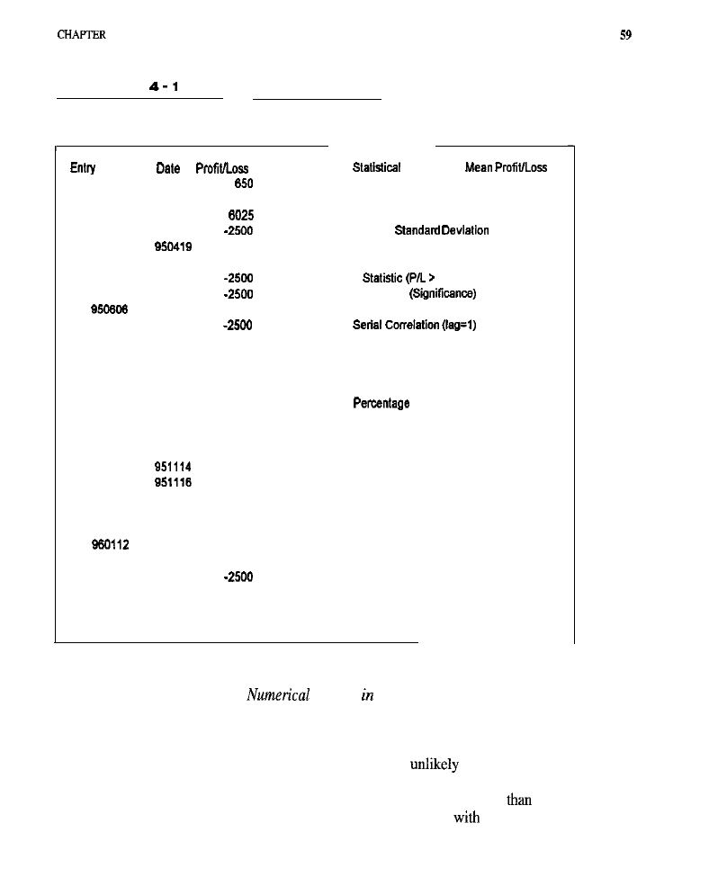
4
Statistics
T A B L E
T r a d e s f r o m t h e S & P 5 0 0 D a t a S a m p l e o n W h i c h t h e L u n a r M o d e l W a s
V e r i f i e d
Date Exit
Cumulative
8 5 0 2 0 7
8 5 0 2 2 1
8 8 8 2 5
8 5 0 2 2 1
950223
-2500
6 6 3 2 5
950309
950323
9 2 3 5 0
9 5 0 3 2 3
950324
8 9 8 5 0
9 5 0 4 0 7
-2500
a 7 3 5 0
9 5 0 4 2 1
850424
-2500
8 4 8 5 0
8 5 0 5 0 8
850516
8 2 3 5 0
850523
9 5 0 5 2 4
7 9 8 5 0
8 5 0 6 0 9
-2500
7 7 3 5 0
850620
050622
74050
850704
850718
4400
7 9 2 5 0
850719
950725
-2500
7 6 7 5 0
850603
950618
2575
7 9 3 2 5
850816
9 5 0 9 0 1
25
7 8 3 5 0
8 5 0 9 0 1
850816
1 0 4 7 5
8 9 8 2 5
9 5 0 9 1 8
950829
-2600
8 7 3 2 5
851002
951003
-2500
8 4 6 2 5
851017
851016
-2550
a 2 2 7 5
8 5 1 0 3 1
3150
8 5 4 2 5
951114
-2500
8 2 9 2 5
951128
9 5 1 2 1 4
6760
8 9 6 7 5
951214
8 5 1 2 2 8
5 2 5 0
9 4 9 2 5
851228
8 6 0 1 0 9
-2500
9 2 4 2 5
8601 I7
-2500
6 9 9 2 5
860128
860213
1 8 7 0 0
1 0 8 6 2 5
860213
860213
1 0 6 1 2 5
960227
960227
-2500
103’325
Additional rows follow but are not shown in the table.
Analyses of
Sample Size
47.0000
Sample Mean
974.4681
Sample
6091.1028
Expected SD of Mean
0 8 8 . 4 7 8 7
T
0)
1.0868
Probability
0 . 1 3 9 2
0.2120
Associated T Statistic
1.4301
Probability (Significance)
0 . 1 5 7 2
Number Of Wlns
16.0000
Of Wins
0 . 3 4 0 4
Upper 98% Bound
0 . 5 3 1 8
L o w e r 8 9 % B o u n d
0 . 1 7 0 2
(Microsoft’s Excel spreadsheet provides a function to obtain probabilities based on
the t-distribution.
Recipes
C provides the incomplete beta function,
which is very easily used to calculate probabilities based on a variety of distribu-
tions, including Student’s t.) The cumulative t-distribution calculation yields a figure
that represents the probability that the results obtained from the trading system were
due to chance. Since this figure was small, it is
that the results were due to
capitalization on random features of the sample. The smaller the number, the more
likely the system performed the way it did for reasons other
chance. In this
instance, the probability was 0.1392; i.e., if a system
a true (population) profit
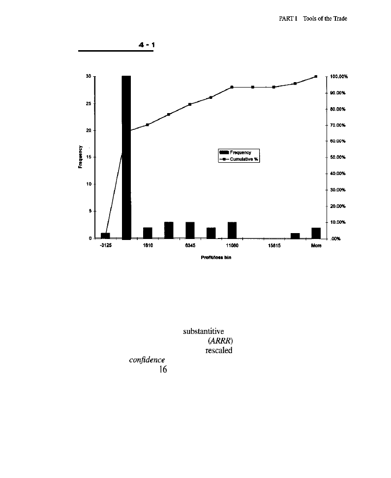
F I G U R E
Frequency and Cumulative Distribution for In-Sample Trades
of $0 was
repeatedly
tested
on independent samples, only about 14% of the time
would it show a profit as high as that actually
observed.
Although the t-test was, in this example, calculated for a sample of trade prof-
it/loss figures, it could just as easily have been computed for a sample of daily
returns. Daily returns were employed in this way to calculate the probabilities
referred to in discussions of the
tests that appear in later chapters. In
fact, the annualized risk-to-reward ratio
that appears in many of the tables
and discussions is nothing more than a
t-statistic based on daily returns.
Finally, a
interval on the probability of winning is estimated. In
the example, there were
wins in a sample of 47 trades, which yielded a per-
centage of wins equal to 0.3404. Using a particular inverse of the cumulative bino-
mial distribution, upper 99% and lower 99% boundaries are calculated. There is a
99% probability that the percentage of wins in the population as a whole is
between 0.1702 and 0.5319. In Excel, the CRITBINOM function may be used in
the calculation of confidence intervals on percentages.
The various statistics and probabilities computed above should provide the
system developer with important information regarding
the behavior of the trad-
ing model-that is, if the assumptions of normality and independence are met and

CHAPTER 4 Statistics
6 1
if the sample is representative. Most likely, however, the assumptions underlying
the t-tests and other statistics are violated; market data deviates seriously from the
normal distribution, and trades are usually not independent. In addition, the sam-
ple might not be representative. Does this mean that the statistical evaluation just
discussed is worthless? Let’s consider the cases.
What
if
the Distribution Is Not Normal? An assumption in the t-test is that the
underlying distribution of the data is normal. However, the distribution of
profit/loss figures of a trading system is anything but normal, especially if there
are stops and profit targets, as can be seen in Figure
which shows the distrib-
ution of profits and losses for trades taken by the lunar system. Think of it for a
moment. Rarely will a
greater than the profit target occur. In fact, a lot
of trades are going to bunch up with a profit equal to that of the profit target. Other
trades
going to bunch up where the
loss is set, with losses equal to that;
and there will be trades that will fall somewhere in between, depending on the exit
method. The shape of the distribution will not be that of the bell curve that describes
the normal distribution. This is a violation of one of the assumptions underlying the
t-test. In this case, however, the Central Limit
Theorem comes to the rescue. It states
that as the number of cases in the sample increases, the distribution of the sample
mean approaches normal. By the time there is a sample size of 10, the errors result-
ing from the violation of the normality assumption will be small, and with sample
sizes greater than 20 or 30, they will have little practical significance for inferences
regarding the mean. Consequently, many statistics can be applied with reasonable
assurance that the results will be meaningful, as long as the sample size is adequate,
as was the case in the example above,
had an of 47.
What
if
There Is Serial Dependence. A more serious violation, which makes
the above-described application of the t-test not quite cricket, is
depen-
dence,
which is when cases constituting a sample (e.g., trades) are not statistical-
ly independent of one another. Trades come from a time series. When a series of
trades that occurred over a given span of dates is used as a sample, it is not quite
a
random sample. A truly random sample would mean that the 100 trades were
randomly taken from the period when the contract for the market started (e.g.,
1983 for the S&P 500) to far into the future; such a sample would not only be less
likely to suffer from serial dependence, but be more representative of
popula-
tion from which it was drawn. However, when developing trading systems, sam-
pling is usually done from one narrow point in time; consequently, each trade may
be correlated with those adjacent to it and so would not be independent,
The practical effect of this statistically is to reduce the
sample size.
When trying to make inferences, if there is substantial serial dependence, it may
be as if the sample contained only half or even one-fourth of the actual number of
trades or data points observed. To top it off, the extent of serial dependence can-
not definitively be determined. A rough
however, can be made. One

such guestimate may be obtained by computing a simple lag/lead
serial correla-
tion: A correlation is computed between the profit and loss for Trade and the
profit and loss for Trade + I, with ranging from
1
to
In the
example, the
serial correlation was 0.2120, not very high, but a lower number would be prefer-
able. An associated t-statistic may then be calculated along with a statistical sig-
nificance for the correlation In the current case, these statistics reveal that if there
really were no serial correlation in the population, a correlation as large as the one
obtained from the sample would only occur in about 16% of such tests.
Serial dependence is a serious problem. If there is a substantial amount of it,
it would need to be compensated for by treating the sample as if it were smaller
than it actually is. Another way to deal with the effect of serial dependence is to
draw a random sample of trades from a larger sample of trades computed over a
longer period of time. This would also tend to make the sample of trades more rep-
resentative of the population,
What
Change?
When developing trading systems, a third assump-
tion of the t-test may be inadvertently violated. There are no precautions that can
be taken to prevent it from happening or to compensate for its occurrence. The rea-
son is that the population from which the development or verification sample was
drawn may be different from the population from which future trades may be taken.
This would happen if the market underwent
some
real structural or other change.
As mentioned before, the population of trades of a system operating on the S&P
500 before 1983 would be different from the population after that year since, in
1983, the options and futures started trading on the S&P 500 and the market
changed. This sort of thing can devastate any method of evaluating a trading sys-
tem. No matter how much a system is back-tested, if the market changes before
trading begins, the trades will not be taken from the same market for which the sys-
tem was developed and tested; the system will fall apart. All systems, even cur-
rently profitable ones, will eventually succumb to market change. Regardless of the
market, change is inevitable. It is just a question of when it will happen. Despite
this grim fact, the use of statistics to evaluate systems remains essential, because if
the market does not change substantially shortly after trading of the system com-
mences, or if the change is not sufficient to grossly affect the system’s performance,
then a reasonable estimate of expected probabilities and returns can be calculated,
Example 2: Evaluating the In-Sample Tests
How can a system that has been fit to a data sample by the repeated adjustment of
parameters (i.e., an optimized system) be evaluated? Traders frequently optimize
systems to obtain good results. In this instance, the use of statistics is more impor-
tant than ever since the results can be analyzed, compensating for the multiplicity
of tests being performed as part of the process of optimization. Table 4-2 contains
the profit/loss figures and a variety of statistics for the in-sample trades (those

taken on the data sample used to optimize the system). The system was optimized
on data from
through
Most of the statistics in Table 4-2 are identical to those in Table 4-1, which
was associated with Example 1. Two additional statistics (that differ from those in
the first example) are labeled “Optimization Tests Run” and “‘Adjusted for
Optimization.” The first statistic is simply the number of different parameter com-
binations tried, i.e., the total number of times the system was run on the data, each
time using a different set of parameters. Since the lunar system parameter,
was
stepped from 1 to 20 in increments of 1, 20 tests were performed; consequently,
there were 20 t-statistics, one for each test. The number of tests
is used to
an adjustment to the probability or significance obtained from the best t-statistic
T r a d e s f r o m t h e S & P 5 0 0 D a t a S a m p l e o n W h i c h t h e L u n a r M o d e l
W a s O p t i m i z e d
800417
800516
800516
900522
900702
800814
900702
900828
800811
8 0 , 2 2 5
-2875
-2500
-2700
8125
-875
-2500
910322
810408
-2.500
3800

computed on the sample: Take 1, and subtract from it the statistical significance
obtained for the best-performing test. Take the resultant number and raise it to the
power (where = the number of tests
Then subtract that number from
1. This provides the probability of finding, in a sample of tests (in this case,
at least one t-statistic as good as the one actually obtained for the optimized solu-
tion. The uncorrected probability that the profits observed for the best solution were
due to chance was less than
a fairly significant result, Once adjusted for mul-
tiple tests, i.e., optimization, the statistical significance does not appear anywhere
near as good. Results at the level of those observed could have been obtained for
such an optimized system 3 1% of the time by chance alone. However, things are
not quite as bad as they seem. The adjustment was extremely conservative and
assumed that every test was completely independent of every other test. In actual
fact, there will be a high serial correlation between most tests since, in many trad-
ing systems, small changes in the parameters produce relatively small changes in
results. This is exactly like serial dependence in data samples: It reduces the
effective population size, in this case, the effective number of tests run. Because
many of the tests are correlated, the 20 actual tests probably correspond to about
to 10 independent tests. If the serial dependence among tests is considered, the
adjusted-for-optimization probability would most likely be around 0.15, instead of
the 0.3 104 actually calculated. The nature and extent of serial dependence in the
multiple tests are never known, and therefore, a less conservative adjustment for
optimization cannot be directly calculated, only roughly reckoned.
Under certain circumstances, such as in multiple regression models, there are
exact mathematical formulas for calculating statistics that incorporate the fact that
parameters are being tit, i.e., that optimization is occurring, making corrections for
optimization unnecessary.
Interpreting the Example Statistics
In Example 1, the verification test was presented. The in-sample optimization run
was presented in Example 2. In the discussion of results, we are returning to the nat-
ural order in which the tests were run, i.e., optimization first, verification second.
Optimization
Results.
Table 4-2 shows the results for the in-sample period. Over
the 5 years of data on which the system was optimized, there were 118 trades
118). the mean or average trade yielded about $740.97, and the trades were
highly variable, with a sample standard deviation of around
i.e., there
were many trades that lost several thousand dollars, as well as trades that made
many thousands. The degree of profitability can easily be seen by looking at the
profit/loss column, which contains many $2,500 losses (the stop got hit) and a sig-
nificant number of wins, many greater than $5,000, some even greater than
$10,000. The expected standard deviation of the mean suggests that if samples of
this kind were repeatedly taken, the mean would vary only about one-tenth as
much as the individual trades, and that many of the samples would have mean
profitabilities in the range of $740 $350.
The t-statistic for the best-performing system from the set of optimization
was 2.1118, which has a statistical significance of 0.0184. This was a fairly
strong result. If only one test had been run (no optimizing), this good a result would
have been obtained (by chance alone) only twice in 100 tests, indicating that the
system is probably capturing some real market inefficiency and has some chance of
holding up. However, be warned: This analysis was for the best of 20 sets of para-
meter
tested. If corrected for the fact that 20 combinations of parameter
ues were tested, the adjusted statistical significance would only be about 0.3 1, not
very good; the performance of the system could easily have been due to chance.
Therefore, although the system may hold up, it could also, rather easily, fail.
The serial correlation between trades was only 0.0479, a value small enough
in the present context, with a significance of only 0.6083. These results strongly
suggest that there was no meaningful serial correlation between trades and that the
statistical analyses discussed above are likely to be correct.
There were 58 winning trades in the sample, which represents about a 49%
win rate. The upper 99% confidence boundary was approximately 61% and the
lower 99% confidence boundary was approximately
suggesting that the true
percentage of wins in the population has a 99% likelihood of being found between
those two values. In truth, the confidence region should have been broadened by
correcting for optimization; this was not done because we were not very con-
cerned about the percentage of wins.
Results.
Table 4-1, presented earlier, contains the data and statistics
for the out-of-sample test for the model. Since all parameters were already fixed,
and only one test was conducted, mere was no need to consider optimization or its
consequences in any manner. In the period from
to
were 47
trades. The average trade in this sample yielded about $974, which is a greater
average profit per trade than in the optimization sample! The system apparently
did maintain profitable behavior.
At slightly over $6,000, the sample standard deviation was almost double
that of the standard deviation in me optimization sample. Consequently, the stan-
dard deviation of the sample mean was around $890, a fairly large standard error
of estimate; together with the small sample size, this yielded a lower t-statistic
than found in the optimization sample and, therefore, a lowered statistical signifi-
cance of only about 14%. These results were neither very good nor very bad:
There is better than an 80% chance that the system is capitalizing on some real
(non-chance) market inefficiency. The serial correlation in the test sample, however,
was quite a bit higher than in the optimization sample and was significant, with a
probability of 0.1572; i.e., as large a serial correlation as this would only be
expected about 16% of the time by chance alone, if no true (population) serial cor-
relation was present. Consequently, the t-test on the
figures has likely

overstated the statistical significance to some degree (maybe between 20 and
30%). If the sample size was adjusted downward the right amount, the t-test prob-
ability would most likely be around 0.18, instead of the 0.1392 that was calculat-
ed. The confidence interval for the percentage of wins in the population ranged
from about 17% to about 53%.
Overall, the assessment is that the system is probably going to hold up in the
future, but not with a high degree of certainty. Considering there were two inde-
pendent tests--one showing about a 31% probability (corrected for optimization)
that the profits were due to chance, the other showing a statistical significance of
approximately 14% (corrected to 18% due to the serial correlation), there is a good
chance that the average population trade is profitable and, consequently, that the
system will remain profitable in the future.
OTHER STATISTICAL TECHNIQUES AND THEIR
USE
The following section is intended only to acquaint the reader with some other sta-
tistical techniques that are available. We strongly suggest that a more thorough study
be undertaken by those serious about developing and evaluating trading systems.
Genetically Evolved Systems
We develop many systems using genetic algorithms. A
(cri-
terion used to determine whether a model is producing the desired outcome) is
total net profit of the system. However, net profit is not the best measure of system
quality! A system that only trades the major crashes on the S&P 500 will yield a
very high total net profit with a
high percentage of winning trades. But who
knows if such a system would hold up? Intuitively, if the system only took two or
three trades in 10 years, the probability seems very low that it would continue to
perform well in the future or even take any more trades. Part of the problem is that
net profit does not consider the number of trades taken or their variability.
An alternative fitness function that avoids some of the problems associated
with net profit is the t-statistic or its associated probability. When using the t-sta-
tistic as a fitness function, instead of merely trying to evolve the most profitable
systems, the intention is to genetically evolve systems that have the greatest like-
lihood of being profitable in the future or, equivalently, that have the least likeli-
hood of being profitable merely due to chance or curve-fitting. This approach
works fairly well. The t-statistic factors in profitability, sample size, and number
of trades taken. All things being equal, the greater the number of trades a system
takes, the greater the t-statistic and the more likely it will hold up in the future.
Likewise, systems that produce more consistently profitable trades with less vari-
ation are more desirable than systems that produce wildly varying trades and will

yield higher t-statistic values. The t-statistic incorporates many of the features that
the quality of a trading model into one number that can be maximized by a
genetic algorithm.
Multiple Regression
Another statistical technique frequently used is multiple regression. Consider
intermarket analysis: The purpose of intermarket analysis is to find measures of
behaviors in other markets that are predictive of the future behavior of the market
being studied. Running various regressions is an appropriate technique for ana-
lyzing such potential relationships; moreover, there are excellent statistics to use
for testing and setting confidence intervals on the correlations and regression
(beta) weights generated by the analyses. Due to lack of space and the limited
scope of this chapter, no examples are presented, but the reader is referred to
Myers
a good basic text on multiple regression.
A problem with most textbooks on multiple regression analysis (including
the one just mentioned) is that they do not deal with the issue of serial correlation
in time series data, and its effect on the statistical inferences that can be made from
regression analyses using such data. The reader will need to take the effects of
serial correlation into account: Serial correlation in a data sample has the effect of
reducing the effective sample size, and statistics can be adjusted (at least in a
rough-and-ready manner) based on this
Another trick that can be used in
some cases is to perform some transformations on
original data series to make
the time series more “stationary” and to remove the unwanted serial correlations.
Monte Carlo Simulations
One powerful, unique approach to making statistical inferences is known as the
Carlo
Simulation,
which involves repeated tests on synthetic data that are
constructed to have the properties of samples taken from a random population.
Except for randomness, the synthetic data are constructed to have the basic char-
acteristics of the population from which the real sample was drawn and about
which inferences must be made. This is a very powerful method. The beauty of
Monte Carlo Simulations is that they can be performed in a way that avoids the
dangers of assumptions (such as that of the normal distribution) being violated,
which would lead to untrustworthy results.
Out-of-Sample Testing
Another way to evaluate a system is to perform
out-of-sample testing.
Several time
periods are reserved to test a model that has been developed or optimized on some
other time period. Out-of-sample testing helps determine how the model behaves

on data it had not seen during optimization or development. This approach is
strongly recommended. In fact, in the examples discussed above, both in-sample
and out-of-sample tests were analyzed. No corrections to the statistics for the
process of optimization are necessary in out-of-sample testing. Out-of-sample and
multiple-sample tests may also provide some information on whether the market
has changed its behavior over various periods of time.
Walk-Forward Testing
In walk-forward testing, a system is optimized on several years of data and then
traded the next year. The system is then
on several more years of data,
moving the window forward to include the year just traded. The system is then
traded for another year. This process is repeated again and again, “walking for-
ward”
through the
data
series. Although very computationally intensive, this is an
excellent way to study and test a trading system. In a sense, even though opti-
mization is occurring, all trades are taken on what is essentially out-of-sample test
data. All the statistics discussed above, such as
t-tests, can be used on
forward test results in a simple manner that does not require any corrections for
optimization. In addition, the tests will very closely simulate the process that
occurs during real trading--first optimization occurs, next the system is traded on
data not used during the optimization, and then every so often the system is
timized to update it. Sophisticated developers can build
optimization process
into the system, producing what might be called an “adaptive” trading model.
Meyers (1997) wrote an article illustrating the process of walk-forward testing.
C O N C L U S I O N
In
the
course of developing trading systems, statistics help the trader quickly reject
models exhibiting behavior that could have been due to chance or to excessive
curve-fitting on an inadequately sized sample. Probabilities can be estimated, and
if it is found that there is only a very small probability that a model’s performance
could be due to chance alone, then the trader can feel more confident when actu-
ally trading the model.
There are many ways for the trader to use and calculate statistics. The cen-
tral theme is the attempt to make inferences about a population on the basis of
samples drawn from that population.
Keep in mind that when using statistics on the kinds of data faced by traders,
certain assumptions will be violated. For practical purposes, some of the violations
may not be too critical; thanks to the Central Limit Theorem, data that are not nor-
mally distributed can usually be analyzed adequately for most needs. Other viola-
tions that are more serious (e.g., ones involving serial dependence) do need to
be
taken
into account, but rough-and-ready rules may be used to reckon corrections

to the probabilities. The bottom line: It is better to operate with some information,
even knowing that some assumptions may be violated, than to operate blindly.
We have glossed over many of the details, definitions, and reasons behind the
statistics discussed above. Again, the intention was merely to acquaint the reader
with some of the more frequently used applications. We suggest that any commit-
ted trader obtain and study some good basic texts on statistical techniques.

P A R T I I
The Study of Entries
Introduction
n
section, various entry methods arc systematically evaluated. The focus is
on which techniques provide good entries and which do not. A good entry is
important because it can reduce exposure to risk and increase
likelihood that a
trade will be profitable. Although it is sometimes possible to make a profit with a
bad entry (given a sufficiently good exit), a good entry gets the trade started on the
right foot.
WHAT CONSTITUTES A GOOD ENTRY?
A good
is one that initiates a trade at a point of low potential risk and high
potential reward. A point of low risk is usually a point from which there is little
adverse excursion before the market begins to move in the trade’s favor. Entries
that yield small adverse excursions on successful trades are desirable because they
permit fairly tight stops to be set, thereby minimizing risk. A good entry should
also have a high probability of being followed quickly by favorable movement in
the market. Trades that languish before finally taking off tie up money that might
be better used elsewhere; not only do such trades increase market exposure, but
they waste margin and lead to
trading or portfolios. Perfect
entries would involve buying the exact lows of bottoming points and selling the
exact highs of topping points. Such entries hardly ever occur in the real world and
are not necessary for successful trading. For trading success it is merely necessary
that entries, when coupled with reasonable exits, produce trading systems that
have good overall performance characteristics.

ORDERS USED IN ENTRIES
Entries may be executed using any of several kinds of orders, including stop
orders, limit orders, and market orders.
Stop Orders
A stop order enters a market that is already moving in the direction of the trade.
A buy or sell is triggered when the market rises above a buy stop or falls below a
sell stop; this characteristic often results in stop orders being used
trend-fol-
lowing entry models. A nice feature of a stop order is that the market must be mov-
ing in a favorable direction at the time of entry. Because of this, the order itself can
act as a
“filter” of the signals generated by the entry model. If a par-
ticular entry happens to be a good one,
will cause the trade to quickly
profitable
hardly any adverse excursion,
On the negative side, an entry executed on a stop order may experience con-
siderable slippage, especially in fast moves, and the market will be bought high or
sold low. Consider the case in which prices begin to move rapidly in favor of a
trade: Buying or selling into such movement is like jumping onto an accelerating
train and is likely to result in large amounts of slippage; the faster the move, the
greater the slippage.
is the difference between the price at which the stop
is set and the price at which it is actually tilled. Because slippage eats into the
profit generated by the trade, it is undesirable. The most unpleasant situation is
when the entry order gets tilled far past the stop, just as the market begins to
reverse! Because buying or selling takes place on a stop, the market entry occurs
significantly into any move and at a relatively poor price.
Limit Orders
In contrast to a stop order, a
order
results in entry when the market moves
against the direction of the trade. A limit order is an order to buy or to sell at a
specified price or better. For a buy limit to be filled, the market must move below
the limit price; for a sell order, the market must move above the limit price. At least
in the short term, buying or selling takes place against the trend. The count&rend
nature of a limit order and the fact that the market may never move to where the
order can be tilled are the primary disadvantages. However, when working with
predictive, countertrend entry models, the countertrend nature of the limit order
may not be a disadvantage at all. The advantage of a limit order is that there is no
slippage and that entry takes place at a good, known price.
Market Orders
A
order
is a simple order to buy or sell at the prevailing market price. One
positive feature of a market order is that it will be executed quickly after being

placed; indeed, many exchanges require market orders to be tilled within a few
minutes at most. Stop or limit orders, on the other hand, may sit for some time
before market activity triggers a till. Another benefit is guaranteed execution:
After placing a market order, entry into the trade will definitely take place. The
drawback to the market order is that slippage may occur. However, in contrast to
the stop order, the slippage can go either way-sometimes in the trade’s favor,
sometimes against it--depending on market movement and execution delay.
Selecting Appropriate Orders
Determining which kind of order to use for an entry must include not only con-
sideration of the advantages and disadvantages of the various kinds of orders, but
also the nature of the model that generates
entry signals and its theory regard-
ing market behavior.
If the entry model predicts turning points slightly into the future, a limit
order may be the most appropriate, especially if the entry model provides some
indication of the price at which the turning point will occur. If the entry model
contains specification of price, as do systems based on critical retracement levels,
entry on a limit (with a tight money management exit stop) is definitely the way
to go: A bounce from the retracement level can be expected, and the limit order
will enter at or near the retracement level, resulting in a trade that either quickly
turns profitable (if the market has responded to the critical level as expected) or is
stopped out with a very small loss.
If the entry model requires some kind of confirmation before entry that the
market is moving in the appropriate direction, a stop order might be the best
choice. For example, a breakout system can be naturally married to a stop-based
entry. If the market moves in a favorable direction and passes the breakout thresh-
old price (the same price at which the entry stop is set), entry will occur automat-
ically, and it will be possible to capture any ensuing move. If the breakout price is
not penetrated, the stop will not be triggered and no entry will take place. In this
example, the entry order actually becomes part of the entry model or system.
Market orders are most useful when the entry model only provides timing
information and when the cost (in terms of slippage and delay) of confirming the
entry with a stop order is too great relative to the expected per-trade profit. A mar-
ket order is also appropriate when the timing provided by the system is critical.
For some models, it would make sense to place a stop or a limit order and then, if
the order is not filled within a specified period of time, to cancel the order and
replace it
a market order.
When developing an entry model, it is often worthwhile to examine various
entry orders to determine which are most manageable and which perform best.
The original entry model will probably need modification to make such tests pos-
sible, but the outcome may prove worth the trouble. Examples of various entry

systems tested using these three types of orders (entry at open, on limit, and on
stop) appear throughout the study of entries.
E N T R Y T E C H N I Q U E S C O V E R E D I N T H I S B O O K
This part of the book explores entry techniques that range from trend-following to
countertrend, from endogenous to exogenous, from traditional to exotic, and from
simple to complex. Since
are an infinite number of entry models, spatial lim-
itations forced us to narrow our focus and discuss only a subset of the possibili-
ties. We attempted to cover popular methods that are frequently discussed, some
of which have been around for decades, but for which there is little objective, sup-
portive evidence. We will systematically put these models to the test to see how
well they work. We have also tried to expand upon some of our earlier, published
studies of entry models in which readers (primarily of
Analysis of Stocks
and Commodities) have expressed great interest.
Breakouts and Moving Averages
Traditional trend-following entry models that employ breakouts and moving aver-
ages are examined in Chapters 5 and 6, respectively.
Breakout
are simple and
intuitively appealing: The market is bought when prices break above an upper band
or threshold. It is sold short when prices break below a lower band or threshold.
Operating this way, breakout entries are certain to get the trader on-board any large
market movement or trend. The trend-following entries that underlie many popular
trading systems are breakout entries. Breakout models differ from one another main-
ly in how the threshold bands are computed and the actual entry is achieved.
Like breakouts, moving averages are alluring in their simplicity and are
extremely popular among technical traders. Entries may be generated using mov-
ing averages in any of several ways: The market may be entered when prices cross
over a moving average, when a faster moving average crosses a slower one, when
the slope of a moving average changes direction, or when prices pull back to a mov-
ing-average line as they might to lines of support or resistance. Additional variety
is introduced by the fact that there are simple moving averages, exponential mov-
ing averages, and triangular moving averages, to mention only a few. Since the
entry models of many trading systems employ some variation of breakouts or mov-
ing averages, it seems important to explore these techniques in great detail.
Oscillators
Oscillators are indicators that tend to fluctuate quasi-cyclically within a limited
range. They are very popular among technical traders and appear in most charting
packages. Entry models based on oscillators are “endogenous” in nature (they do

not require anything but market data) and are fairly simple to implement, charac-
teristics they share with breakout and moving-average models. However, breakout
and moving-average models tend to enter the market late, often too late, because
they are designed to respond to, rather than anticipate, market behavior. In con-
trast, oscillators anticipate prices by identifying turning points so that entry can
occur before, rather than after, the market moves. Since they attempt to anticipate
prices, oscillators characteristically generate countertrend entries.
Entries are commonly signaled by divergence between an oscillator and
price. Divergence is seen when prices form a lower low but the oscillator forms a
higher low, signaling a buy; or when prices form a higher high but the oscillator
forms a lower high, signaling the time to sell short.
A signal line is another way to generate entries. It is calculated by taking a
moving average of the oscillator, The trader buys when the oscillator crosses above
the signal line and sells short when it crosses below. Although typically used in
“trading range” markets for countertrend entries, an oscillator is sometimes
employed in a trend-following manner: Long or short positions might be entered
when the Stochastic oscillator climbs above 80 or drops below 20, respectively.
Entry models that employ such classic oscillators as Lane’s Stochastic, Williams’s
RSI, and
MACD are studied in Chapter 7.
Seasonality
Chapter 8 deals with seasonality, which is construed in different ways by dif-
ferent traders. For our purposes,
is defined as cyclic or recurrent
phenomena that are consistently linked to the calendar, specifically, market
behavior affected by the time of the year or tied to particular dates. Because
they are predictive (providing trading signals weeks, months, or years ahead),
these models are countertrend in nature. Of the many ways to time entries that
use seasonal rhythms, two basic approaches will be examined: momentum and
crossover. The addition of several rules for handling confirmations and inver-
sions will also be tested to determine whether they would produce results bet-
ter than the basic models.
Lunar and Solar Phenomena
Do lunar and solar events influence the markets? Is it possible for an entry model to
capitalize on the price movements induced by such influences? The moon’s role in
the instigation of tides is undisputed. Phases of the moon correlate with rainfall and
with certain biological rhythms, and they influence when farmers plant crops. Solar
phenomena, such as solar flares and sunspots, are also known to impact events on
earth. During periods of high solar activity, magnetic storms occur that can disrupt
power distribution systems, causing serious blackouts. To assume that solar and
lunar phenomena influence the markets is not at all unreasonable; but how might
these influences be used to generate predictive,
entries?
Consider the lunar rhythm: It is not hard to define a model that enters the
ket a specified number of days before or after either the full or new moon. The same
applies to solar activity: An entry can be signaled when the sunspot count rises above
some threshold or falls below another threshold. Alternatively, moving averages of
solar activity can be computed and crossovers of these moving averages used to time
market entries. Lunar cycles, sunspots, and other planetary rhythms may have a real,
albeit small, impact on the markets,
impact that might be profitable with a prop-
erly constructed entry model. Whether lunar and solar phenomena actually affect the
markets sufficiently to be taken advantage of by an astute trader is a question for an
empirical investigation, such as that reported in Chapter 9.
Cycles and Rhythms
Chapter 10 explores cycles and rhythms as a means of timing entries into the mar-
ket. The idea behind the use of cycles to time the market is fundamentally simple:
Extrapolate observed cycles into the future, and endeavor to buy the cycle lows
and sell short the cycle highs. If the cycles are sufficiently persistent and accu-
rately extrapolated, excellent countertrend entries should be the result. If not, the
entries are likely to be poor.
For a very long time, traders have engaged in visual cycle analysis using
charts, drawing tools, and, more recently, charting programs. Although cycles can
be analyzed visually, it is not very difficult to implement cycle recognition and
analysis algorithms in software. Many kinds of algorithms are useful in cycle
analysis-everything from counting the bars between tops or bottoms, to fast
Fourier transforms
and maximum entropy spectral analyses (MESA
S
).
Getting such algorithms to work well, however, can be quite a challenge; but hav-
ing reliable software for cycle analysis makes it possible to build objective,
based entry models and to test them on historical data using a trading simulator.
Whether detected visually or by some mathematical algorithm, market
cycles come in many forms. Some cycles are exogenous, i.e., induced by external
phenomena, whether natural or cultural. Seasonal rhythms, anniversary effects,
and cycles tied to periodic events (e.g., presidential elections and earnings reports)
fall into the exogenous category: these cycles are best analyzed with methods that
take the timing of the driving events into account. Other cycles are
endogenous;
i.e., their external driving forces are not apparent, and nothing other than price data
is needed to analyze them. The 3-day cycle occasionally observed in the S&P 500
is example of an endogenous cycle, as is an S-minute cycle observed by the
authors in S&P 500 tick data. Programs based on band-pass filters (Katz and
McCormick, May 1997) and maximum entropy (e.g., MESA96 and
are good at finding endogenous cycles.

We have already discussed the exogenous seasonal cycles, as well as lunar
and solar rhythms. In Chapter 10, endogenous cycles are explored using a sophis-
ticated wavelet-based, band-pass filter model.
Neural Networks
As discussed in Chapter 11, neural
network
technology is a form of
intelli-
gence (or AI) that arose from endeavors to emulate the kind of information
and decision making that occurs in living organisms. Neural networks (or “nets”)
are components that learn and that are useful for pattern recognition, classification,
and prediction. They can cope with probability estimates in uncertain situations and
with “fuzzy” patterns, i.e., those recognizable by eye but difficult to
using
rules. Nets can be used to directly detect
points or forecast price changes,
in an effort to obtain good, predictive,
entry models. They can also vet
entry signals generated by other models. In addition, neural network technology can
help integrate information from both endogenous sources, such as past prices, and
exogenous sources, such as sentiment
seasonal data, and intermarket variables,
in a way that benefits the trader. Neural networks can even be trained to recognize
visually detected patterns in charts, and then serve as pattern-recognition blocks with-
in traditional rule-based systems (Katz and McCormick, November 1997).
Genetically Evolved Entry Rules
Chapter 12 elaborates a study (Katz and McCormick, December 1996) demon-
strating that genetic evolution can be used to create stable and profitable rule-
based entry models. The process involves putting together a set of model
fragments, or “rule templates,” and allowing a genetic algorithm (GA) to combine
and complete these fragments to achieve profitable entries. The way the method-
ology can discover surprising combinations of rules that consider both
and exogenous variables, traditional indicators, and even nontraditional
elements (e.g., neural networks) in making high-performance entry decisions will
be examined. Evolutionary model building is one of the most advanced,
edge, and unusual techniques available to the trading system developer.
S T A N D A R D I Z E D E X I T S
To study entries on their own, and to do so in a way that permits valid comparisons
of different strategies, it is essential to implement a
exit that will be
held constant across various tests; this is an aspect of the scientific method that
was discussed earlier. The scientific method involves an effort to hold everything,
except that which is under study, constant in order to obtain reliable information
about the element being manipulated.

The standardized exit, used for testing entry models in the following chapters,
incorporates the three functions necessary in any exit model: getting out with a prof-
it when the market moves sufficiently in the trade’s favor, getting out with a limited
loss when the market moves against the trade, and getting out from a languishing
market after a limited time to conserve margin and reduce exposure. The standard
exit is realized using a combination of a
stop order,
a
order, and a
market order.
Stop and limit orders are placed when a trade is entered. If either order is
filled within a specified interval, the trade is complete, the remaining order is can-
celed, and no additional orders are placed. If, after the allotted interval, neither the
stop nor limit orders are filled, they are canceled and a market order is placed to
force an immediate exit from the trade. The stop order, called a money
stop, serves to close out a losing position with a small, manageable loss. Taking a
profit is accomplished with the limit order, also
a
target. Positions that
go nowhere are closed out by the market order. More elaborate exit strategies are
discussed in “Part III: The Study of Exits,” where the entries are standardized.
Money management stops and profit target limits for the standardized exits
are computed using
units, rather than fixed dollar amounts, so that they
will have reasonably consistent meaning across eras and markets. Because, e.g., a
$1,000 stop would be considered tight on today’s S&P 500 (yet loose on wheat),
fixed-dollar-amount stops cannot be used when different eras and markets are
being studied. Volatility units are like standard deviations, providing a uniform
scale of measurement. A stop, placed a certain number of volatility units away
from the current price, will have a consistent probability of being triggered in a
given amount of time, regardless of the market. Use of standardized measures per-
mits meaningful comparisons across markets and times.
E Q U A L I Z A T I O N O F D O L L A R V O L A T I L I T Y
Just as exits must be held constant across entry models, risk and reward potential,
as determined by
dollar
volatility (different from raw volatility, mentioned above),
must be equalized across markets and eras. This is done by adjusting the number
of contracts traded. Equalization of risk and reward potential is important because
it makes it easier to compare the performance of different entry methods over
commodities and time periods. Equalization is essential for portfolio simulations,
where each market should contribute in roughly equal measure to the performance
of the whole portfolio. The issue of dollar volatility equalization arises because
some markets move significantly more in dollars per unit time than others. Most
traders are aware that markets vary greatly in size, as reflected in differing margin
requirements, as well as in dollar volatility. The S&P 500, for example, is recog-
nized as a “‘big” contract, wheat as a “small” one; many contracts of wheat would
have to be traded to achieve the same bang as a single S&P 500 contract. Table II-l
shows, broken down by year and market, the dollar volatility of a single contract
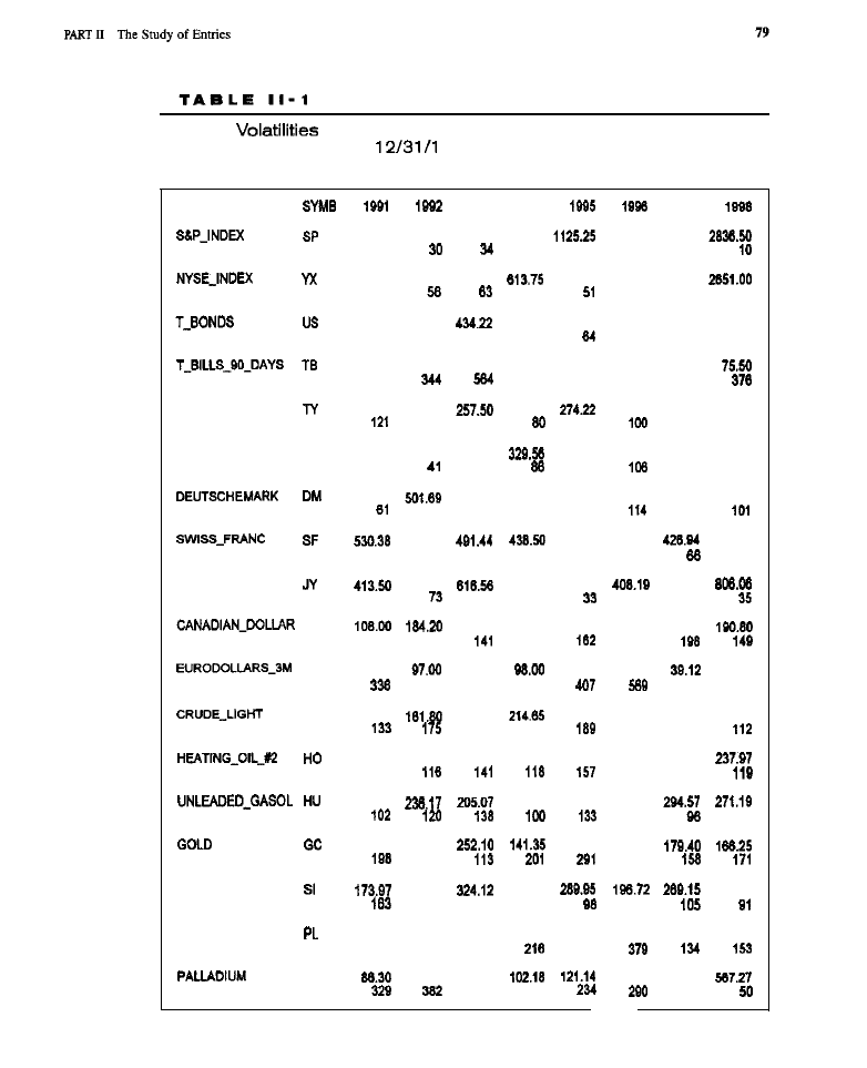
Dollar
(First Line) and Number of Contracts Equivalent to
10 New S&P 500s on
998 (Second Line) Broken Down by
Market and Year
N A M E
, 8 8 3
1884
, 8 8 7
1183.50
848.37
823.80
1124.37
1888.00 4188.50
2 4
2 5
2 5
1 4
7
825.50
MD.75
452.80
558.00
887.87
1888.82
4 5
4 8
2 8
1 4
1 1
348.13
342.81
510.00
438.84
475.83
388.58
488.84
8 1
8 3
8 5
5 8
8 0
7 7
8 0
82.81
82.38
50.25
88.25
12.38
84.83
48.12
342
288
382
518
511
TEN-YEAR-NOTES
2 3 5 . 3 ,
3 0 2 . 3 4
3 5 2 . 5 0
2 8 3 . 8 8
204.10
216.41
8 4
H O
1 0 3
1 3 8
1 0 3
B R I T I S H - P O U N D
B P
8 4 2 . 8 8
8 8 7 . 8 1
5 3 4 . 8 8
3 5 8 . 7 5
2 8 8 . 5 2
3 1 1 . 8 8
3 3 8 . 8 1
4 4
5 3
7 8
7 5
8 4
4 8 7 . 3 ,
3 8 7 . 0 0
9 9 8 . 3 7
4 7 8 . 0 0
2 4 7 . 8 8
5 3 2 . 3 1
2 8 2 . 0 8
5 7
1 3
8 4
8 0
8 5
8 8 1 . 5 8
6 6 8 . 7 5
3 8 7 . 8 ,
4 1 8 . 1 2
5 3
4 3
5 8
8 5
4 2
7 3
8 8
J A P A N E S E - Y E N
3 8 8 . 8 8
5 3 1 . W
5 7 2 . 2 5
5 8 8 . 5 0
8 8
4 8
8 3
8 8
4 8
C D
M O . 8 0
1 3 8 . 7 5
1 1 5 . 2 5
8 3 . 0 5
143.50
2 8 3
1 5 4
2 0 4
3 0 5
E D
8 4 . 3 8
4 4 . 1 3
8 8 . 1 5
4 8 . 8 1
5 0 . 1 5
2 8 2
843
2 8 8
7 2 5
5 0 0
C L
2 1 3 . 2 5
1 7 8 . 8 0
1 5 0 . 1 0
244.85
2 3 2 . 0 0
2 5 2 . 6 0
1 5 8
1 3 2
8 2
1 2 2
2 8 8 . 0 5
2 4 4 2 1
2 0 0 . 8 0
2 3 8 . 7 8
1 8 0 . 8 2
3 7 4 . 9 ,
2 5 8 . 8 7
1 0 5
7 8
H O
2 7 5 . 8 3
282.10
214.05
3 7 7 . 0 3
7 5
1 0 5
143.55
1 2 3 . 9 0
97.45
8 4 . 8 0
2 2 8
3 3 5
S I L V E R
H 3 . 7 5
2 1 1 . 2 5
310.52
249
8 8
1 0 5
1 4 4
PLATINUM
1 3 1 . 0 0
1 2 8 . 7 3
145.40
131.53 135.45
7 4 . 8 3
2 1 2 . 1 2
1 8 5 . 5 2
2 0 7
2 2 0
1 8 1
2 0 8
P A
7 4 . 2 5
1 2 8 . 8 3
9 7 . 8 5
3 0 1 . 8 2
2 2 0
2 7 8
8 2
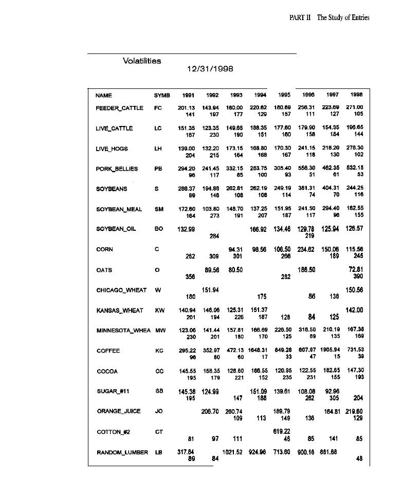
T A B L E I I - 1
Dollar
(First Line) and Number of Contracts Equivalent to
10 New S&P 500s on
(Second Line) Broken Down by
Market and Year (Continued)
80.81
213
103.10
01.04
78.00
317
157.31
187
130.08
218
352
137.00
207
170
2.38
70.00
370
102.50
21,
100.50
223.00
124
221.81
121
152
330.13
338.87
225 224
ea.38
328
207.84
188
227.3,
200
183.42
130.33
227
203
217.40
251.10
208.01
130
137
172
351.12
201.05
254.05 351.75
332.50 201.30 332.05
81
338.40
583.44
2 8
3,
40
3 2
4 2

and
the number
of contracts that would have to
be
traded to equal the dollar
volatility of 10 new S&P 500 contracts at the end of 1998.
For the current studies, the average daily volatility is computed by taking a
moving average of the absolute
of the difference between the current
close and the previous one. The average daily volatility is then multiplied by the dol-
lar value of a point, yielding the desired average daily dollar volatility. The dollar
value of a point can be obtained by dividing the dollar value of a
(a market’s
minimum move) by the size of a tick (as a decimal number). For the new S&P 500
contract, this works out to a value of $250 per point (tick
size =
To obtain the number of contracts of a target market that would have to be traded to
equal the dollar volatility of new S&P 500 contracts on
the dollar
volatility of the new S&P 500
is
divided by the dollar volatility of the target market;
the result is multiplied
by
10 and rounded to the nearest positive integer.
All the simulations reported in this book assume that trading always involves
the same amount of dollar volatility. There is no compounding; trade size is not
increased with growth in account equity. Equity curves, therefore, reflect returns
from an almost constant investment in terms of risk exposure. A constant-investment
model
avoids the serious problems that arise when a compounded-investment
approach is used in simulations with such margin-based instruments as futures. With
margin-based securities, it is difficult to define return except in absolute dollar
amounts or in relationship to margin requirements or risk, simple ratios cannot be
used. In addition, system equity may occasionally dip below zero, creating problems
with the computation of logarithms and further obscuring the meaning of ratios.
However, given a constant investment (in terms of volatility exposure), monthly
measured in dollars will have consistent significance over time, t-tests on
average dollar return values
be valid (the annualized risk-to-reward ratio used to
assess performance in the tests that follow is actually a
t-statistic),
and
it
will be easy to see if a system is getting better or worse over time, even if there are
periods of negative equity. The use of a fixed-investment model, although carried out
more rigorously here by maintaining constant risk, rather than a constant number of
contracts, is in accord with what has
appeared
in other
books
concerned with futures
trading. This does not
that a constant dollar volatility portfolio must always be
traded. Optimal and other reinvestment strategies can greatly improve overall
returns; they just make simulations much more difficult to interpret. In any case,
such strategies can readily and most appropriately be tested after the fact using
equity and trade-by-trade data generated by a fixed-investment simulation.
BASIC TEST PORTFOLIO AND PLATFORM
A
of futures markets is employed for all tests
of
entry methods
reported in this section. The reason for a standard portfolio is the
as that for
a fixed-exit strategy or dollar volatility equalization: to ensure
that
test results will

be valid, comparable, and consistent in meaning. All price series were obtained
from Pinnacle Data in the form of continuous contracts, linked and back-adjusted
as suggested by Schwager (1992). The standard portfolio is composed of the fol-
lowing markets (also see Table II-l): the stock indices (S&P 500, NYFE), interest
rate markets (T-Bonds,
T-Bills,
Notes), currencies (British Pound,
Deutschemark, Swiss Franc, Japanese Yen, Canadian Dollar, Eurodollars), energy
or oil markets (Light Crude,
Heating Oil, Unleaded Gasoline), metals (Gold,
Silver, Platinum, Palladium), livestock (Feeder Cattle, Live Cattle, Live Hogs,
Pork Bellies), traditional
(Soybeans, Soybean Meal Soybean Oil,
Corn, Oats, Wheat), and other miscellaneous commodities (Coffee, Cocoa, Sugar,
Orange Juice,
Cotton, Random Lumber). Selection of markets was aimed at
creating a high level of diversity and a good balance of market types.
the
stock index bond, currency, metal, energy, livestock, and grain markets all have
representation, several markets (e.g., the Nikkei Index and Natural Gas) would
have improved the balance of the portfolio, but were not included due to the lack
of a sufficient history. In the chapters that follow,
models
tested both on
the complete standard portfolio and on the individual markets that compose it.
Since a good system should be able to trade a variety of markets with the same
parameters, the systems were not optimized for individual markets, only for
entire portfolio. Given the number of data points available, optimizing on specific
markets could lead to undesirable curve-fitting.
Unless otherwise noted, quotes from August 1, 1985, through December 31,
1994, are
as in-sample or optimization data, while those from January 1,
1995, through February
are used for out-of-sample verification. The num-
ber of contracts traded is adjusted to achieve a constant effective dollar volatility
across all markets and time periods; in this way, each market and time period is
more comparable with other markets and periods, and contributes about equally to
the complete portfolio in terms of potential risk and reward. All tests use the same
standardized exit technique to allow meaningful performance comparisons
between entry methods.

C H A P T E R
Breakout Models
A
breakout
enters the market long when prices break above an upper band
or threshold, and enters short when they drop below a lower band or threshold.
Entry models based on breakouts range from the simple to the complex, differing
primarily in how the placement of the bands or thresholds is determined, and in
how entry is achieved.
KINDS OF BREAKOUTS
Breakout models are very popular and come in many forms. One of the oldest is the
used by chartists. The chartist draws a descending
line that serves as
upper threshold: When prices break above the trendline, a long
position is established; if the market has been rising, and prices break below an
ascending trendline, a short entry is taken. Support and resistance lines, drawn using
angles or Fibonacci
can also serve as breakout thresholds.
Historically,
breakout
employing support and resistance lev-
els determined by previous highs and lows, followed chart-based methods. The
trader buys when prices rise above the highest of the last bars (the upper chan-
nel), and sells when prices fall below the lowest of the last bars (the lower chan-
nel). Channel breakouts are easily mechanized and appeal to traders wishing to
avoid the subjectivity of drawing trendlines or
angles on charts.
More contemporary and sophisticated than channel breakouts are
volatility
breakout models where the points through which the market must move to trigger
long or short positions are based on
volatility bands. Volatility bands are placed a
certain distance above and below some measure of current value (e.g., the most
recent closing price), the distance determined by recent market volatility: As

volatility increases, the bands expand and move farther away from the current
price; as it declines, the bands contract, coming closer to the market. The central
idea is statistical: If the market moves in a given direction more than expected
from normal jitter (as reflected in the volatility measurement), then some force
may have impinged, instigating a real trend worth trading. Many $3,000 systems
sold since the late 1980s employed some variation on volatility breakouts,
Breakout models also differ in how and when they enter the market. Entry
can occur at the open or the close, requiring only a simple market order. Entry
inside the bar is accomplished with stops placed at the breakout thresholds. A
more sophisticated way to implement a breakout entry is to buy or sell on a limit,
attempting to enter the market on a small pull-back, after the initial breakout, to
control
and achieve entry at a better price.
CHARACTERISTICS OF BREAKOUTS
Breakouts are intuitively appealing. To get from one place to another, the market
must cross all intervening points. Large moves always begin with small moves.
Breakout systems enter the market on small moves, when the market crosses one of
the intermediate points on the way to its destination: they buy into movement.
Breakout models arc, consequently, trend-following. Another positive characteristic
of breakout models is that, because they buy or sell into momentum, trades quickly
become profitable. Sometimes a very tight stop-loss can be set, an approach that can
only be properly tested with
tick-level data. The intention would be to enter
on a breakout and to then set a very tight stop loss, assuming momentum at the
breakout will carry the market sufficiently beyond the stop-loss to prevent it from
being triggered by normal market fluctuations; the next step would be to exit with a
quick profit, or ratchet the protective stop to break-even or better. Whether a profit
can be taken before prices reverse depends on the nature of the market and whether
momentum is strong enough to carry prices into the profit zone.
On the downside, like many trend-following models, breakouts enter the
market late-sometimes too late, after a move is mostly over. In addition, small
moves can trigger market entries, but never become the large moves necessary for
profitable trading. Since breakout systems buy or sell into trends, they are prone
to
slippage; however, if well-designed and working according to theory,
occasional strong trends should yield highly profitable trades that make up for the
more frequent (but smaller) losers. However, the consensus is that, although their
performance might have been excellent before massive computational power
became inexpensive and widespread, simple breakout methods no longer work
well. As breakout systems were developed, back-tested, and put on-line, the mar-
kets may have become increasingly efficient with respect to them. The result is
that the markets’ current noise level around the prices where breakout thresholds
are often set may be causing many breakout systems to generate an excessive

ber of bad entries; this is especially likely in active, volatile markets, e.g., the S&P
500 and T-Bonds. Finally, it is easy to encounter severe slippage (relative to the
size of a typical trade) when trying to implement trading strategies using breakout
entries on an intraday time frame; for longer term trading, however, breakout entry
strategies may perform acceptably.
A well-designed breakout model attempts to circumvent the problem of mar-
ket noise to the maximum extent possible. This may be accomplished by placing
the thresholds at points unlikely to be reached by movements that merely represent
random or nontrending market activity, but that are likely to be reached if the mar-
ket has developed a significant and potentially profitable trend. If the bands are
placed too close to the current price level, a large number of false breakouts (lead-
ing to whipsaw trades) will occur: Market noise will keep triggering entries, first in
one direction, then in the other. Because such movements do not constitute real
trends with ample follow-through, little profit will be made; instead, much heat (in
the form of commissions and slippage) will be generated and dissipate the trader’s
capital. If the bands are set too wide, too far away from the prevailing price, the sys-
tem will take few trades and entry into the market will be late in the course of any
move; the occasional large profit from a powerful trend will be wiped out by the
losses that occur on market reversals. When the thresholds are set appropriately
(whether on
basis of
volatility bands, or support and resistance),
breakout entry models can, theoretically, be quite effective: Frequent, small losses,
occurring because of an absence of follow-through on noise-triggered entries,
should be compensated for by the substantial profits that accrue on major thrusts.
To reduce false breakouts and whipsaws, breakout systems are sometimes
married to indicators, like Welles Wilder’s “directional movement index”
that supposedly ascertain whether the market is in a trending or nontrending mode.
If the market is not trending, entries generated by the breakouts are ignored; if it
is,
are taken. If popular trend indicators really work, marrying one to a break-
out system (or any other trend-following model) should make the trader rich:
Whipsaw trades should be eliminated, while trades that enter into strong trends
should yield ample profits. The problem is that trend indicators do not function
well, or tend to lag the market enough to make them less than ideal.
TESTING BREAKOUT MODELS
Tests are carried out on several different breakout models, trading a diversified
portfolio of commodities, to determine how well breakout entries perform. Do
they still work? Did they ever? Breakout models supposedly work best on com-
modities with persistent trends, traditionally, the currencies. With appropriate fil-
tering, perhaps these models can handle a wider range of markets. The
investigations below should provide some of the answers. The standard portfolio
and exit strategy were used in all tests (see “Introduction” to Part for details).

CHANNEL BREAKOUT ENTRIES
The initial tests address several variations of the channel breakout entry. First
examined are close-only channel breakout models, in which the price channels or
bands are determined using only closing prices. A model involving breakouts that
occur beyond the highest high or lowest low will also be studied. In these mod-
els, the price channels approach the traditional notion of support and resistance.
Close-Only Channel Breakouts
Test I: Close-Only Channel Breakout with
on Market Order at Next
Open, No
Costs.
The rules are: “If the current position is either
short or flat and the market closes above the highest close of the last days, then
buy tomorrow’s open.” Likewise, “If the current position is either long or flat
and the market closes below the lowest close of the preceding days, then sell
(go short at) tomorrow’s open.” The channel breakout entry model has only one
parameter, the look-back
The number of contracts to buy or sell
was chosen to produce, for the market being traded, an effective dollar volatili-
ty approximately equal to that of two new S&P 500 contracts at the end of 1998.
Exits occur either when a breakout entry reverses an existing position or
when the standard exit closes out the trade, i.e., when a money management stop
is triggered, a profit target is hit, or the position has been open more than a speci-
fied number of days (bars), whichever comes first. The money management stop
is computed as the entry price plus (for short positions) or minus (for long posi-
tions) some multiple (a parameter,
of the 50-bar average true range. Profit
target limits are at the entry price plus (long) or minus (short) another multiple
of the same average true range. Finally, an “exit at close” order (a form of
market order) is posted when a position has been held for more than a specified
number of days
All exit orders are “close-only,” i.e., executed only at
the close: this restriction avoids ambiguous simulations when testing entries with
limits or stops. Were exits not restricted to the close, such cases would
involve the posting of multiple intrabar orders. Simulations become indeterminate
and results untrustworthy when multiple intrabar orders are issued: The course of
prices throughout the period represented by the bar, and hence the sequence of
order executions, is unknown.
The average
range (a measure of volatility) is calculated as the mean of
the true range of each of a specified number of previous bars (in this case, 50). The
true range is the highest of the day’s high minus the day’s low, the day’s high
minus the previous day’s close, or the previous day’s close minus the day’s low.
Below is a C+ + implementation of the close-only channel breakout entry
model mated with the standard exit strategy. When calculating the number of con-
tracts, no correction is explicitly made for the S&P 500 split. The new contract is

treated as identical to the old one, both by the simulator and by the code. All sim-
ulations are, nevertheless, correct under the assumption that the trader (not the
simulator) trades two new contracts for every old contract: The simulator is
instructed to sell half as many
contracts as it should, but treats these contracts
as twice their current size. Limit-locked days
detected by range checking: A
zero range (high equal to the low) suggests poor liquidity, and a possibly
locked market. Although this detection scheme is not ideal, simulations using it
resemble results obtained in actual trading. Compiling the information from
exchanges needed to identify limit-locked days would have been almost impossi-
ble; therefore, the zero-range method is used. The code allows re-entry into per-
sistent trends as long as new highs or lows are made.
declare local
variables
static
static

process next
The code was compiled and linked with the development shell and associat-
ed libraries; in
this is called “verifying” a system. Using develop-
ment shell commands, the look-back parameter was brute-force optimized. The
best solution (in terms of the risk-to-reward ratio) was then verified on out-of-sam-
ple data. Optimization involved stepping the entry model look-back
from 5 to
100, in increments of 5. The stop-loss parameter
was fixed at 1 (repre-
senting 1 volatility, or average true range, unit), the profit target
at 4 (4
units), and the maximum holding period
at 10 days. These values are
used for the standard exit parameters in all tests of entry methods, unless

wise specified. To provide a sense of scale when considering the stop-loss and
profit target used in the standard exit, the S&P 500 at the end of 1998 had an aver-
age true range of 17.83 points, or about $4,457 for one new contract. For the fist
test, slippage and commissions were set to zero.
For such a simple system, the results are surprisingly good: an annual return
of 76% against maximum drawdown. All look-back parameter values were prof-
itable; the best in terms of risk-to-reward ratio was 80 days. A t-test for daily
returns (calculated using the risk-to-reward ratio) reveals the probability is far less
than one in one-thousand that chance explains the performance; when corrected
for the number of tests in the optimization, this probability is still under one in
one-hundred. As expected given these statistics, profits continued out-of-sample.
Greater net profits were observed from long trades (buys), relative to short ones
(sells), perhaps due to false breakouts on the short side occasioned by the constant
decay in futures prices as contracts neared expiration. Another explanation is that
commodity prices are usually more driven by crises and shortages than by excess
supply. As with many breakout systems, the percentage of winners was small
with large profits from the occasional trend compensating for frequent
small losses. Some may find it hard to accept a system that takes many losing
trades while waiting for the big winners that make it all worthwhile.
Portfolio equity for the best in-sample look-back rose steadily both in- and
out-of-sample; overoptimization was not au issue. The equity curve suggests a
gradual increase in market efficiency over time, i.e., these systems worked better
in the past. However, the simple channel breakout can still extract good money
from the markets. Or can it? Remember Test 1 was executed without transaction
costs. The next simulation includes slippage and commissions.
Test 2: Close-Only Channel Breakout with Entry at Next Open, Transaction
Costs Assumed.
This test is the same as the previous one except that slippage
(three ticks) and commissions ($15 per round turn) are now considered. While
this breakout model was profitable without transaction costs, it traded miserably
when realistic costs were assumed. Even the best in-sample solution had nega-
tive returns (losses); as might be expected, losses continued in the out-of-sam-
ple period. Why should relatively small commission and slippage costs so
devastate profits when, without such costs, the average trade makes thousands of
dollars? Because, for many markets, trades involve multiple contracts, and slip-
page and commissions occur on a per-contract basis. Again, long trades and
longer look-backs were associated with higher profits. The model was mildly
profitable in the
but lost money thereafter. Considering the profitable
results of the previous test, it seems the model became progressively more
unable to overcome the costs of trading. When simple computerized breakout
systems became the rage in the late
they possibly caused the markets to
become more efficient.

Table 5-l shows the portfolio performance of the close-only channel break-
out system broken down by sample and market
(For information about
various markets and their symbols, see Table II-1 in the “Introduction” to Part II.)
= the total net profit on long trades, in thousands of dollars;
= the
total net profit on short trades, in thousands of dollars;
= annualized
return-on-account;
= associated probability or statistical significance;
=
average
per trade.
Trend-following methods, such as breakouts, supposedly work well on the
currencies. This test confirms that supposition: Positive returns were observed
both in-sample and out-of-sample for several currencies. Many positive returns
were also evidenced in both samples for members of the Oil complex, Coffee,
and Lumber. The profitable performance of the stock indices (S&P 500 and
is probably due to the raging bull of the 1990s. About 10 trades were
taken in each market every year, The percentage of wins was similar to that seen
in Test (about 40%).
Test 3: Close-Only Channel Breakout with Entry on Limit on Next Bar,
Transaction Costs Assumed. To improve model performance by controlling
slippage and obtaining entries at more favorable prices, a limit order was used to
enter the market the next day at a specified price or better. Believing that the mar-
ket would retrace at least 50% of the breakout bar (cb) before moving on, the limit
price
was set to the midpoint of that bar. Since most of the code remains
unchanged, only significantly altered blocks are presented:
Trade entry took place inside the bar on a limit. If inside-the-bar profit target
and stop-loss orders were used, problems would have arisen. Posting multiple
bar orders can lead to invalid simulations: The sequence in which such orders are
tilled cannot be specified with end-of-day data, but they can still strongly affect the
outcome. This is why the standard exit employs orders restricted to the close.
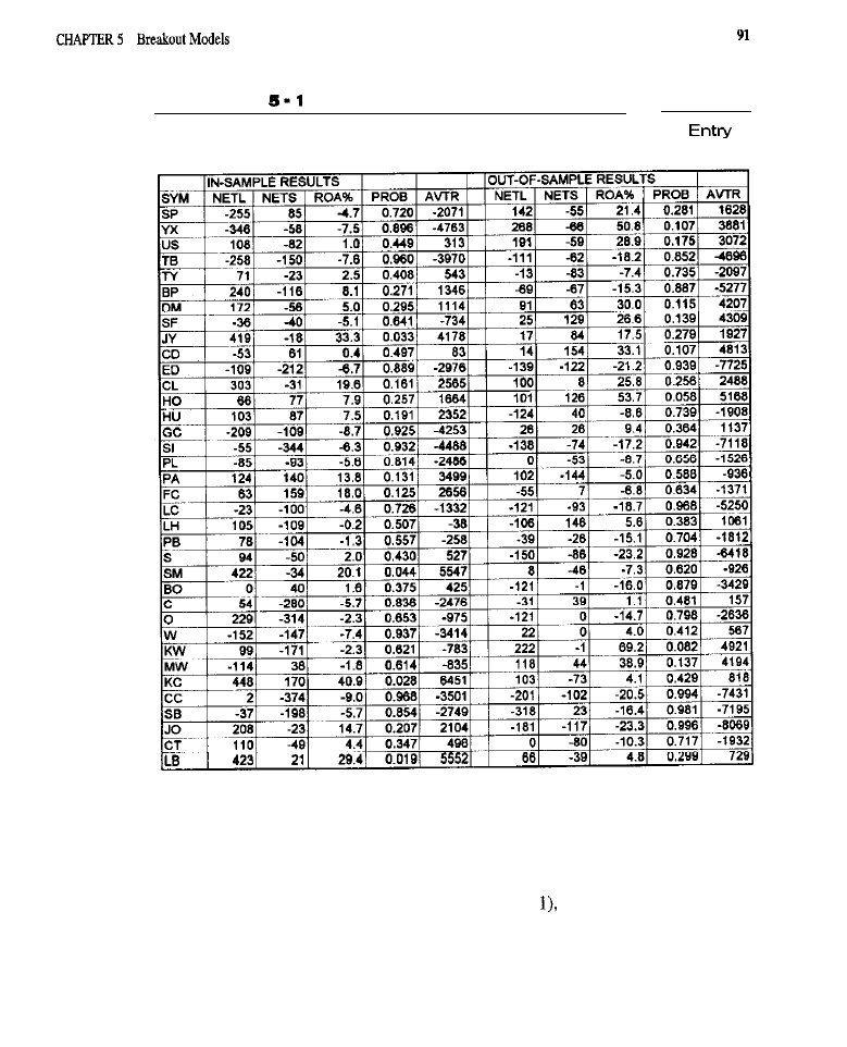
T A B L E
Performance Statistics for Close-Only Channel Breakout with
at Open for All Markets in the Standard Portfolio
As before, the look-back parameter was stepped from 5 to 100, in increments
of 5, and the solution with the best risk-to-reward ratio (and t-test probability) was
selected. Commissions, slippage, exit parameters, and the ability to reenter a con-
tinuing trend (albeit on a pullback), remain unchanged.
With a best look-back of 80 (same as in Test this model returned about
33% annually during the in-sample period. The probability that these returns
were. due to chance is less than 5% when not corrected, or 61% when corrected
for 20 optimization runs. Although profitable in-sample, the statistics suggest the

model may fail in the future: indeed, out-of-sample returns were negative. As in
Tests 1 and 2, trades lasted about seven bars and long trades were more profitable
than short ones. The percentage of winners was 42%. Although the limit entry did
not eliminate the damaging impact of transaction costs, performance improved.
The limit order did not seriously reduce
of trades or cause many prof-
itable trends to be missed, the market pulled back after most breakouts, allowing
entry at more favorable prices. That a somewhat arbitrary, almost certainly
optimal, limit entry strategy could so improve performance is highly encourag-
ing. The equity curve again shows that
kind of system once worked but no
longer does.
Table 5-2 shows that, with few exceptions, there were positive returns for
currencies and oils, both in-sample and out-of-sample, consistent with findings in
earlier tests. Coffee continued to trade well on both samples, and the S&P 500
remained profitable in the verification sample.
Conclusion
A limit-based entry can significantly improve the overall perfor-
mance of a breakout model. Substantial benefit is obtained even with a fairly crude
choice for the limit price. It is interesting that the markets to benefit most from the
use of a limit order for entry were not necessarily those with the lowest dollar
volatilities and implied transaction costs, as had been expected. Certain markets,
like the S&P 500 and Eurodollars, just seem to respond well to limit entries, while
others, such as Cocoa and Live Cattle, do not.
HIGHEST HIGH LOWEST LOW BREAKOUTS
Would placing the thresholds further from current prices reduce whipsaws,
increase winning trades, and improve breakout performance? More stringent
breakout levels are readily obtained by replacing the highest and lowest close from
the previous model with the highest high and lowest low
in the current
model. Defined this way, breakout thresholds now represent traditional levels of
support and resistance: Breakouts occur when previous highs or lows are “taken
out” by the market. One possible way to further reduce spurious breakouts is by
requiring the market to close beyond the bands, not merely to penetrate them at
some point inside the bar. Speeding up system response by using a stop order for
entry, or reducing transaction costs by entering on a pullback with a limit order,
might also improve performance.
Test 4: Close-Only HHLL Breakout with Entry at Open of Next Bar.
This
breakout buys at tomorrow’s open when today’s close breaks above the highest
high of the last days, and sells at tomorrow’s open when today’s close drops
below the lowest low. The look-back (n) is the only model parameter. The
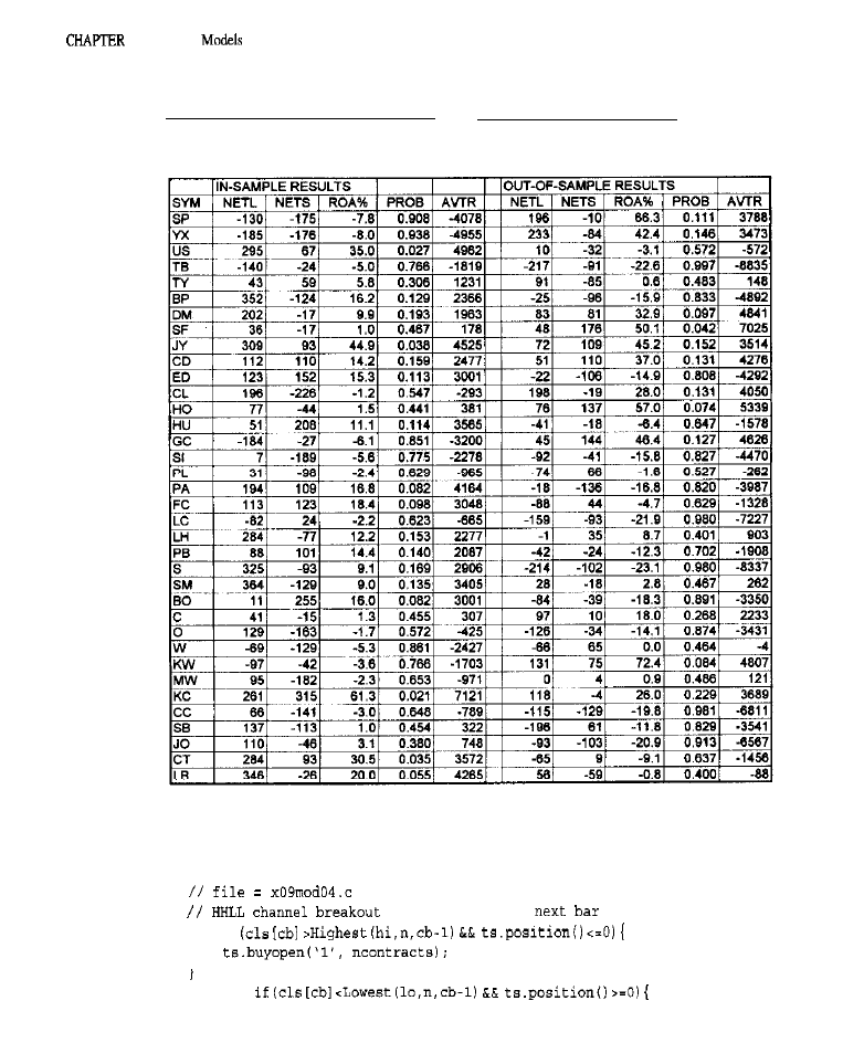
5 Breakout
T A B L E S - 2
Y 3
Performance Statistics for Close-Only Channel Breakout with Entry
at Limit for All Markets in the Standard Portfolio
ty of this model, besides its simplicity, is that no important trend will be
missed, and tomorrow’s trades are fully known after today’s close.
system with entry
on open
i
f
e l s e

Look-backs from
5 to
100
were tested
in steps of 5. On the in-sample data,
the model was profitable for only four of the look-backs. The best results were
obtained with a look-back of 85, where in-sample returns were a mere 1.2% annu-
ally. Given these returns and the associated statistics, it is no surprise that this
model lost 15.9% annually out-of-sample. Winners occurred about 39% of the
time, and long trades were more profitable than short ones in-sample. As in all pre-
vious breakout simulations, the HHLL breakout performed best on the currencies,
the oils,
and
Coffee; it performed worst on metals, livestock, and grains. Equity
shows a model that never performed well, but that now performs disastrously.
The results were slightly better than those for the close-only breakout with
a similar entry at the open; they were not better enough to overcome transaction
costs. In the close-only model, a limit order reduced the cost of failed breakouts
and, thereby, improved performance. Because costs are higher with the HHLL
breakout, due to the more stringent breakout thresholds, a limit entry may pro-
vide a greater boost to performance. A limit entry for a breakout model also side-
steps the flurry of orders that often hit the market when entry stops, placed at
breakout thresholds, are triggered. Entries at such times are likely to occur at
unfavorable prices. However, more sophisticated traders will undoubtedly “fade”
the movements induced by the entry stops placed by more
traders, driving
prices back. An appropriate limit order may be able to enter on the resultant pull-
back at a good price. If the breakout represents the start of a trend, the market is
likely to resume its movement, yielding a profitable trade; if not, the market will
have less distance to retrace from the price at entry, meaning a smaller loss. Even
though the HHLL breakout appears only marginally better than the close-only
breakout thus far, the verdict is not yet in; a limit entry may produce great
improvement.
The annualized return-on-account is used as an index of performance in
these discussions and the risk-to-reward ratio is rarely mentioned, even though the
probability statistic (a t-statistic) is computed using that measure. The
reward ratio and return-on-account are very highly correlated with one another:
They are almost interchangeable as indicators of model efficacy. Since it is easier
to understand. the annualized return-on-account is referred to more
Test 5: Close-Only HHLL Breakout with
on Limit on Next Bar.
For the
close-only channel breakout,
use
of a limit order for entry greatly improved per-
formance. Perhaps a limit entry could similarly benefit the HHLL breakout model.
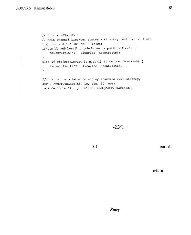
For the sake of consistency with the model examined in Test 3, the limit price is
set to the mid-point of the breakout bar.
The look-back parameter was stepped through the same range as in previous
tests. All look-backs produced positive returns. The best in-sample results were
with a look-back of 85, which yielded a return of 36.2% annually; the probability
is less than 2% (33% when corrected for multiple tests) that this was due to
chance. In-sample, long positions again yielded greater profits than short posi-
tions. Surprisingly, out-of-sample, the short side produced a small profit, while the
long side resulted in a loss! With a return of
out-of-sample performance
was poor, but not as bad as for many other systems tested. In-sample, there were
43% wins and the average trade produced an $1,558 profit; out-of-sample, 41%
were winners and the average trade lost $912.
The equity curve in Figure
may seem to contradict the negative
sample returns, but the trend in the out-of-sample data was up and on par with the
trend in the latter half of the in-sample period. The apparent contradiction results
from a bump in the equity curve at the start of the out-of-sample period.
Nevertheless, the HHLL breakout with entry on a limit (together with the standard
exit) is not a system that one would want to trade after June 1988: The
was
too low relative to the risk represented by the fluctuation of equity above and
below the least-squares polynomial trendline (also shown in Figure 5-l).
All currencies and oils had positive in-sample results. Strong out-of-sample
returns were seen for the Swiss Franc, Canadian Dollar, and Deutschemark, as
well as for Heating Oil and Light Crude; small losses were observed for the British
Pound, Eurodollar, and Unleaded Gasoline. Coffee was profitable in both samples.
Test 6: Close-Only HHLL Breakout with
on
Stop
on
Next Bar.
This
model buys on a stop at a level of resistance defined by recent highs, and sells on
a stop at support as defined by recent lows. Because the occurrence of a breakout
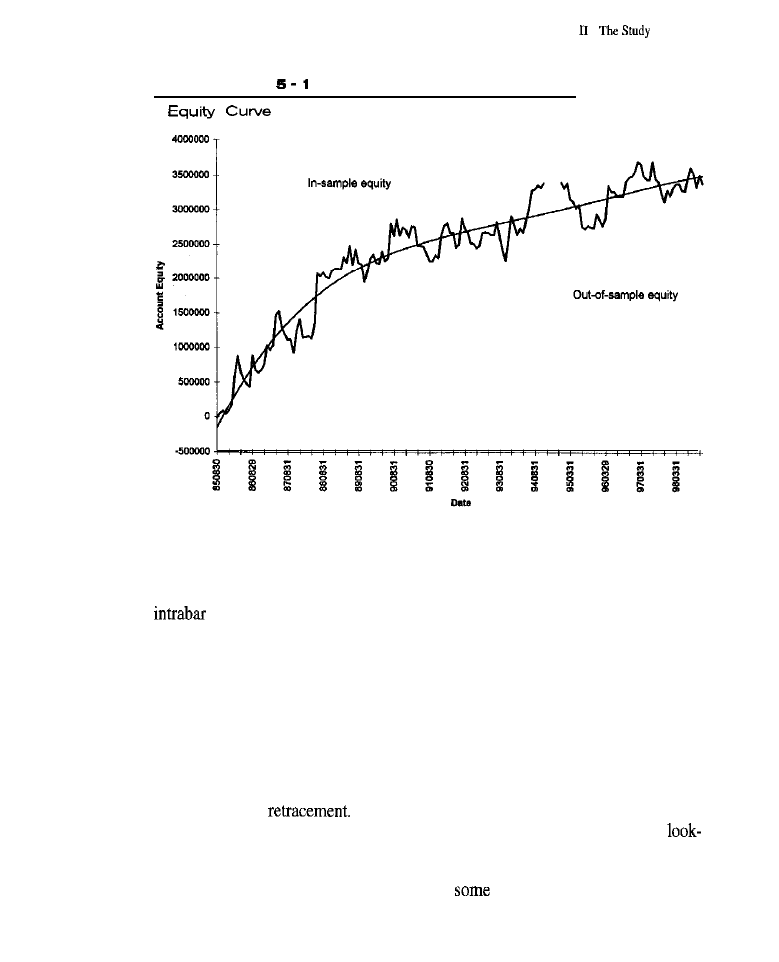
PART
of Entries
F I G U R E
for HHLL Breakout, Entry at Limit
is decided on the entry bar by the stop itself, the highest high and lowest low are
calculated for bars up to and including the current bar. The relative position of the
close, with respect to the breakout thresholds, is used to avoid posting multiple
orders. If the close is nearer to the upper threshold, then the buy stop is
posted; if the close is closer to the lower threshold, the sell stop is posted. Both
orders are never posted together. By implementing the HHLL breakout with stop
orders, a faster response to breakout conditions is achieved; there is no need to
wait for the next bar after a signal is given to enter the market. Entry, therefore,
occurs earlier in the course of any market movement and no move will ever be
missed, as might happen with a limit while waiting for a pull-back that never takes
place. However, the reduced lag or response time may come at a cost: entry at a
less favorable price. There is greater potential for slippage, when buying into
momentum on a stop, and entry takes place at the breakout price, rather than at a
better price on a
The look-back parameter was optimized as usual. The best in-sample
back was 95, with look-backs of 65 through 100 being profitable. Annual returns
were 8.7%. Although the results were better than those for Test 4, they were not
as good as for Test 5. Faster response bought
advantage, but not as much as

waiting for a retracement where entry can occur at a more favorable price. The
percentage of winning trades was 41% and the average trade yielded a $430 prof-
it. Out-of-sample, the picture was much worse, as might be expected given the low
returns and poor statistics on the in-sample data. This model lost an average of
$798 per trade. About 37% of the trades were winners. The model made most of
its profits before June 1988, and lost money after January 1992.
All currencies, except Eurodollars, had positive returns in the optimization peri-
od. In the verification period, the Japanese Yen, Canadian Dollar, and
had solid
in the 30% to 50% range. The model also generated moderate
on the oils. Coffee traded well, with a 21.2% return in-sample and a 61.8%
out-of-sample. Random Lumber also had positive
in both samples.
VOLATILITY BREAKOUT ENTRIES
The next three tests evaluate volatility breakout entry models, in which the trader
buys when prices rise above an upper volatility band, and sells short when they fall
below a lower volatility band. Volatility bands are bands placed above and below
current prices. When volatility increases, the bands expand; when it decreases, they
contract. The balance point around which the bands are drawn may be the most
recent closing price, a moving average, or some other measure of current value.
Test 7:
Breakout
at Next Open.
This model buys at tomor-
row’s open when today’s close pushes above the upper volatility band, and sells
short at the next open when the close drops below the lower volatility band. The
volatility bands are determined by adding to (for the upper band) and subtracting
from (for the lower band) the estimate of current value a multiple (bw) of the
average true range (a measure of volatility). The estimate of value is a
exponential moving average of the closing price. If the moving average
length
is one, this estimate degrades to the closing price on the breakout
or “signal” bar.
Because the volatility breakout model has three parameters, genetic optimiza-
tion was chosen for the current test. Using genetic optimization, the bandwidth para-
meter (bw) was evaluated over a range of 1.5 to 4.5, with a grid size (increment) of
0.1; the period of the average true range
was studied over a range of 5 to SO,
with a grid size of 1; and the moving average length
was examined over a
range of 1 to 25, also with a unit grid size. The genetic optimization was allowed to
for 100 generations. As in all previous tests, the highest attainable risk-to-reward
ratio (or, equivalently, the lowest attainable probability that any profits were due to
chance) on the in-sample or optimization data was sought.
The best in-sample performance was obtained with a bandwidth of 3.8, a
moving average length of 5, and an average true range of 20 bars. With these para-
meters, the annualized return was 27.4%. There was a probability of 5.6% (99.7%

when corrected for
tests or generations) that chance produced the observed
return. Almost every combination of parameters examined generated profits on the
long side and losses on the short side. The average trade for the best parameter set
was held for 6 bars and yielded a profit of $4,675. Only 240 trades were present in
the optimization period, about 45% of which were winners. Compared to previous
tests, the smaller number of trades, and the higher percentage of winners, are
explained by breakout thresholds placed further from current price levels. The aver-
age trade lost $7,371 in the verification sample and only 25% of the 112 trades were
profitable. Both long positions and short positions lost about the same amount.
Almost all gain in equity occurred from August 1987 to December 1988, and
then from December 1992 to August 1993. Equity declined from October 1985
through July 1986, from August 1989 through May 1992, and from May 1995 to
December 1998.
Excessive optimization may have contributed to deteriorated performance in
the verification sample. Nevertheless, given the number of parameters and para-
meter combinations tested, a good entry model should have generated a greater in-
sample return than was seen and better statistics, capable of withstanding
correction for multiple tests without total loss of significance. In other words,
excessive optimization may not be the central issue: Despite optimization, this
model generated poor in-sample returns and undesirably few trades. Like the oth-
ers, this model may simply have worked better in the past.
As before, currencies were generally profitable. Oddly, the oil complex, which
traded profitably in most earlier tests, became a serious loser in this one. Coffee and
Lumber traded well in-sample, but poorly out-of-sample, the reverse of previous
findings. Some of these results might be due to the model’s limited number of trades.
Test 8:
Breakout with Entry on Limit.
This model attempts to estab-
lish a long position on the next bar using a limit order when the close of the cur-
rent bar is greater than the current price level plus a multiple of the average true
range. It attempts to establish a short position on the next bar using a limit order
when the close of the current bar is less than the current price level minus the same
multiple of the average
range. The current price level is determined by an
exponential moving average of length
calculated for the close. The multi-
plier for the average true range is referred to as bw, and the period of the average
true range as
Price for the limit order to be posted on the next bar is set to
the midpoint price of the current or breakout bar. Optimization was carried out
exactly as in Test 7.
For all parameter combinations, long positions were more profitable (or lost
less) than short positions. The best in-sample results were achieved with a band-
width of 3.7, a moving average length of 22, and a period of 41 for the average
true range measure of volatility; these parameter values produced a 48.3% annu-
alized return. Results this good should occur less than twice in one-thousand

experiments; corrected for multiple tests (100 generations), the probability is less
than 13% that the observed profitability was due to chance. On the in-sample data,
1,244 trades were taken, the average trade lasted 7 days, yielded
and was
a winner 45% of the time. Both long and short trades were profitable.
Given the statistics, there was a fair probability that the model would con-
tinue to be profitable out-of-sample; however, this was not the case. The model
lost heavily in the out-of-sample period. Equity rose rather steadily from the
beginning of the sample until August 1990, drifted slowly lower until May 1992,
rose at a good pace until June 1995, then declined. These results primarily
reflect the decreasing ability of simple breakout models to capture profits from
the markets.
All currencies had positive in-sample returns and all, except the British
Pound and Canadian Dollar, were profitable out-of-sample-confirmation that
breakout systems perform best on these markets, perhaps because of their trendi-
ness. Curiously, the currency markets with the greatest returns in-sample are not
necessarily those with the largest returns out-of-sample. This implies that it is
desirable to trade a complete basket of currencies, without selection based on his-
torical performance, when using a breakout system. Although this model per-
formed poorly on oils, it produced stunning returns on Coffee (both samples
yielded greater than 65% annually) and Lumber (greater than 29%).
9:
Breakout
Entry on Stop.
This model enters immediately
at the point of breakout, on a stop which forms part of the entry model. The advan-
tage is that entry takes place without delay: the disadvantage is that it may occur
at a less favorable price than might have been possible later, on a limit, after the
clusters of stops that are often found around popular breakout thresholds have
been taken out. To avoid multiple
orders, only the stop for the band near-
est the most recent closing price is posted; this rule was used in Test 6. The volatil-
ity breakout model buys on a stop when prices move above the upper volatility
band, and sells short when they move below the lower volatility band.
The optimum values for the three model parameters were found with the aid
of the genetic optimizer built into the C-Trader toolkit from Scientific Consultant
Services, Inc. The smallest risk-to-reward ratio occurred with a bandwidth of X.3, a
moving average length of 11, and an average true range of
bars. Despite opti-
mization, this solution returned only 11.6% annually. There were 1,465 trades
taken; 40% were winners. The average trade lasted 6 days and took $931 out of the
market. Only long positions were profitable across parameter combinations.
Both long and short trades lost heavily in the verification sample. There were
610 trades, of which only 29% were winners. The equity curve and other simula-
tion data suggested that deterioration in the out-of-sample period was much
greater for the volatility breakout model with a stop entry than with entry on a
limit, or even at the open using a market order.

Can excessive optimization explain the rapid decay in the out-of-sample
period? No. Optimization may have merely boosted overall in-sample perfor-
mance from terrible to poor, without providing improved out-of-sample perfor-
mance. Optimization does this with models that lack real validity, capitalizing on
chance more than usual. The greater a model’s real power, the more helpful and
less destructive the process of optimization. As previously, the detrimental effects
of curve-fitting are not the entire story: Performance declined well before the
of-sample period was reached. The worsened out-of-sample performance can as
easily be attributed to a continued gain in market efficiency relative to this model
as it can to excessive optimization.
The model generated in-sample profits for the British Pound, Deutschemark,
Swiss Franc, and Japanese Yen; out-of-sample, profits
generated for all of
these markets except the British Pound. If all currencies (except the Canadian
Dollar and Eurodollar) were traded, good profits would have been obtained in both
samples. The Eurodollar lost heavily due to the greater slippage and less favorable
prices obtained when using a stop for entry; the Eurodollar has low dollar volatil-
ity and, consequently, a large number of contracts must be traded, which
ties transaction costs. In both samples, Heating Oil was profitable, but other
members of the oil group lost money. The out-of-sample deterioration in certain
markets, when comparison is to entry on a limit, suggests that it is now more dif-
ficult to enter on a stop at an acceptable price.
VOLATILITY BREAKOUT VARIATIONS
Would restricting breakout models to long positions improve their performance?
How about trading only the traditionally trendy currencies? Would benefit be
derived from a trend indicator to filter out whipsaws? What would happen without
m-entries into existing, possibly stale, trends? The last question was answered by
an unreported test in which entries took place only on breakout reversals. The
results were so bad that no additional tests were completed, analyzed, or reported.
The
three questions, however, are addressed below.
Long Positions Only
In the preceding tests, the long side almost always performed better than the short
side, at least on in-sample data. What if one of the previously tested models was
modified to trade only long positions? Test 10 answers that question.
Test IO:
Breakout with Limit
Only
T h e
best in-sample model (Test 8) was modified to
only long positions. A genetic
algorithm optimized the model parameters. Band-width
was optimized from 1.5
to 4.5, with a grid of 0.1; the period of the average
range
from 5 to 50,
with a grid of 1; and the length of the moving average
from 1 to 25, with a
grid of 1. Optimization was halted after
generations.
In-sample, the model performed well. The best parameter values were: band-
width, 2.6; moving average length, 15; and average true range period,
The best
parameters produced an annualized return of
and a risk-to-reward ratio of
1.17
0.0002; 0.02, corrected). There were 1,263 trades, 48% profitable
(a higher percentage than in any earlier test). The average trade lasted 7 days, with
a $4,100 profit after slippage and commissions. Even suboptimal parameter val-
ues were profitable, e.g., the worst parameters produced a 15.5% return!
Out-of-sample, despite the high levels of statistical significance and the
robustness of the model (under variations in parameter values when tested on
sample data), the model performed very poorly: There were only 35% wins and a
loss of -14.6% annually. This cannot be attributed to in-sample curve-fitting as all
in-sample parameter combinations were profitable. Suboptimal parameters should
have meant diminished, but still profitable, out-of-sample performance. Additional
tests revealed that no parameter set could make this model profitable in the
sample period! This finding rules out excessive optimization as the cause for
of-sample deterioration. Seemingly, in recent years, there has been a change in the
markets that affects the ability of volatility breakout models to produce profits,
even when restricted to long positions. The equity curve demonstrated that the
model had most of its gains prior to June 1988. The remainder of the optimization
and all of the verification periods evidenced the deterioration.
As before, most currencies traded fairly well in both samples. The average
currency trade yielded $5,591 in-sample and $1,723 out-of-sample. If a basket of
oils were traded, profits would be seen in both samples. Coffee was also profitable
in both samples.
Overall, this system is not one to trade today, although it might have made a
fortune in the past; however, there may still be some life in the currency, oil, and
Coffee markets.
Currencies Only
The currency markets are believed to have good trends, making them ideal for
such trend-following systems as breakouts. This belief seems confirmed by the
tests above, including Test 10. Test restricts the model to the currencies.
Test 11:
Breakout with Limit Entry Trading Only Currencies.
This
model is identical to the previous one, except that the restriction to long trades
was removed and a new restriction to trading only currencies was established.
No optimization was conducted because of the small number of markets and,
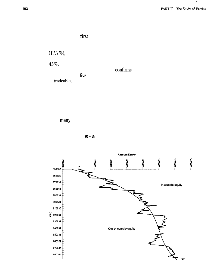
consequently, data points and trades; instead, the best parameters from Test 8
were used here.
This is the
test where a breakout produced clearly profitable results in
both samples with realistic transaction costs included in the simulation! In-sam-
ple, the model returned 36.2% annually. Out-of-sample, the
return was
lower
but still good. There were 268 trades, 48% wins, with an average profit
per trade (in-sample) of 53,977. Out-of-sample, the model took 102
trades, won
and averaged 52,106 per trade.
The equity curve in Figure 5-2
the encouraging results. Almost all equi-
ty was gained in
thrusts, each lasting up to a few months. This model is potential-
ly
especially if the standard exit was replaced with a more effective one.
ADX Trend Filter
One problem with breakouts is the tendency to generate numerous whipsaw trades
in which the breakout threshold is crossed, but a real trend never develops. One
possible solution is to use a trend indicator to filter signals generated by raw break-
outs;
traders do this with the ADX, a popular trend indicator. Test 12 exam-
ines whether Wilder’s ADX is beneficial.
F I G U R E
Equity Curve for HHLL Breakout, Entry on Limit, Currencies Only

Test 12: Volatility Breakout with Limit Entry and Trend Filter.
The same
model from Tests and 11 is used; instead of restriction to long positions or
currencies, the signals are “filtered” for trending conditions using the Average
Directional Movement index (or ADX; Wilder, 1978). By not entering
less markets, whipsaws and languishing trades, and the resultant erosion of
capital, can hopefully be reduced. The ADX was implemented to filter break-
outs as suggested by White (1993). Trending conditions exist as long as the
ADX makes a new 6-bar high, and entries are taken only when trends
exist.
As in previous tests, a genetic algorithm optimized the parameters. All 100
parameter combinations except one produced positive returns in-sample; 88
returned greater than
demonstrating the model’s tolerance of parameter vari-
ation. The best parameters were: bandwidth, 2.6; moving average length, 8; and
average true range period, 34. With these parameters the in-sample return was
68.3%; the probability that such a high return would result from chance was less
than one in two-thousand, or about one in twenty-nine instances when corrected
for optimization. There were 872 trades and 47% wins. The average trade gener-
ated about $4,500 in profit. Out-of-sample the average trade lost $2,415 and only
36% of all trades taken (373) were winners.
return was
one of the
worst out-of-sample performances. The ADX appears to have helped more in the
past than in current times.

Most currencies, Heating Oil, Coffee, Lumber, and
Notes were prof-
itable out-of-sample. The
Kansas Wheat, and
Gold were profitable
out-of-sample, but lost money it-sample. The pattern is typical of what has been
observed with breakout systems, i.e., the currencies, oils, and Coffee tend to be con-
sistently profitable.
S U M M A R Y A N A L Y S E S
Table 5-3 summarizes breakout results broken down by model, sample, and order
type.
ARRR
the annualized risk-to-reward ratio,
ROA
= the annualized return
on account, and
AVTR = the
average trade’s profit or loss.
Breakout Types
In the optimization sample (1985 to 1995). volatility breakouts worked best, the
highest-high/lowest-low breakout fell in-between, and the close-only breakout did
worst: this pattern was consistent across all three order types. In the verification
period (1995 through
the
continued to do slightly
better than the close-only, but the volatility model performed much worse. For rea-
sons discussed earlier, optimization cannot account for the relatively dramatic
deterioration of the volatility breakout in recent years. Perhaps the volatility break
out deteriorated more because of its early popularity. Even the best breakout mod-
els, however, do poorly in recent years.
When broken down by model, three distinct periods were observed in the aver-
aged equity curves. From August 1985 through June 1988, all models were about
equally profitable. From June 1988 to July 1994, the HHLL and close-only models
were flat and choppy. The volatility model showed a substantial gain from August
1992 through July 1994. From July 1994 until December 1998, the HHLL and
close-only breakouts were choppy and slightly down, with the HHLL model some-
what less down than the close-only model; equity for the volatility model declined
significantly.
Entry Orders
Both in- and out-of-sample, and across all models, the limit order provided the
greatest edge; the stop and market-at-open orders did poorly. The benefit of the
limit order for entering the market undoubtedly stemmed from its ability to
obtain entries at more favorable prices, The dramatic impact of transaction costs
and unfavorable entry prices is evident in Tests 1 and 2. Surprisingly, the limit
order even worked with a trend-following methodology like breakouts. It might
be expected that too many good trends would be missed while waiting to enter
on a limit; however, the market pulls back (even after valid breakouts) with

Summary of Breakout Entry Results Arranged for Easy
Comparison
enough frequency to enter on a limit at a better price without missing too many
good trends.
The same three periods, evident when average equity was broken down by
breakout type, appeared when entry orders were analyzed. For the limit and stop
entries, equity surged strongly from August 1985 to June 1988. Equity increased,
but to a lesser extent, with a stop order. For entry at the open and on a stop, equity
was choppy and down-trending from June 1988 to July 1994, when the limit
order modestly gained. From July 1994 to December 1998, equity for entry at the
open mildly declined, the stop evidenced a serious decline, and the limit had no
consistent movement. The stop did better than average during the first period and
much worse than average during the third, more decay in performance over time
occurred with a stop order than with the other orders. In all periods, the limit
order performed best.
When equity was analyzed for all models and order types combined, most of
its gains were in the first period, which covered less than the first third of the
sample period. By the end of this period, more than 70% of the peak equity had

already accumulated. In the second period, equity drifted up a little. In the third
period, equity declined, at
gradually and then, after July 1997, at a faster pace.
Interactions
Interactions seemed strongest between breakout types and time. The most
notable was between volatility breakouts (versus the others) and time
ple versus out-of-sample). Volatility breakouts performed best early on, but
later became the worst. The volatility breakout with stop entry deteriorated
more in recent years than it did with entry on a limit, perhaps due to the com-
mon use of stops for entry in trend-following models. Finally, the
breakout sometimes favored a stop, while the volatility model
never did.
Restrictions and Filters
Restricting trades to long positions greatly improved the performance of the
volatility breakout in-sample, and improved it to some extent out-of-sample.
Breakout models do better on the long side than on the short one. The ADX
trend filter had a smaller benefit in-sample and provided no benefit
sample.
Restricting trading to currencies produced lessened in-sample perfor-
mance, but dramatic improvements out-of-sample. The gain was so great that
the model actually profited out-of-sample, which cannot be said for any of the
other combinations tested! The currencies were not affected by the rising
ciency other markets had to simple breakout systems, perhaps because the cur-
rency markets are huge and driven by powerful fundamental forces. The poorer
in-sample performance can be explained by the reduced number of markets
traded.
Analysis by Market
Net profit and annual return were averaged for each market over all tests. The
culated numbers contained no surprises. Positive returns were seen in both samples
for the Deutschemark, Swiss Franc, Japanese Yen, and Canadian Dollar, and for
Light Crude and Heating Oil. Trading a basket of all six currencies, all three oils, or
both, would have been profitable in both samples. Although no other market group
demonstrated consistent profitability, some individual markets did. In order of min-
imum net profit, Coffee, Live Hogs, and Random Lumber had positive
The S&P 500, NYFE,
Gold, Corn, and the wheats had positive
of-sample returns with in-sample losses. The index markets’ profitability may
have resulted from the strong trends that developed out-of-sample. Positive
sample returns, associated
with
out-of-sample losses, were somewhat more

common; T-Bonds, IO-Year
Palladium, Feeder Cattle, Pork Bellies,
Soybeans, Soybean Meal, Bean Oil, Oats, Orange Juice, and Cotton had this pat-
tern. T-Bills, Silver, Platinum, Live Cattle, Cocoa, and Sugar lost in both sam-
ples. A correlation of 0.15 between net in-sample and net out-of-sample profits
implies markets that traded well in the optimization period tended to trade well
in the verification period.
CONCLUSION
No technique, except restricting the model to the currencies, improved results
enough to overcome transaction costs in the out-of-sample period. Of course,
many techniques and combinations were not tested (e.g., the long-only restriction
was tested only with the volatility breakout and not with the HHLL breakout, a
better out-of-sample performer), although they might have been effective. In both
samples, all models evidenced deterioration over time that cannot be attributed to
overoptimization. Breakout models of the kind studied here no longer work, even
though they once may have. This accords with the belief that there are fewer and
fewer good trends to ride. Traders complain the markets are getting noisier and
more countertrending, making it harder to succeed with trend-following methods.
No wonder the
limit entry works best!
Overall, simple breakout models follow the aforementioned pattern and do
not work very well in today’s
markets. However, with the right combina-
tion of model, entry order, and markets, breakouts can yield at least moderate prof-
its. There are many variations on breakout models, many trend filters beyond the
ADX, and many additional ways to improve trend-following systems that have not
been examined. Hopefully, however, we have provided you with a good overview
of popular breakout techniques and a solid foundation on which to begin your own
investigations.
WHAT HAVE WE LEARNED?
n
If possible, use a limit order to enter the market. The markets are noisy and
usually give the patient trader an opportunity to enter at a better price; this
is the single most important thing one can do to improve a system’s prof-
itability. Controlling transaction costs with limit orders can make a huge
difference in the performance of a breakout model. Even an unsophisticated
limit entry, such as the one used in the tests, can greatly improve trading
results. A more sophisticated limit entry strategy could undoubtedly pro-
vide some very substantial benefits to this kind of trading system.
. Focus on support and resistance, fundamental verities of technical
analysis that are unlikely to be “traded away.” The
low breakout held up better in the tests than other models, even though

it did not always produce the greatest returns. Stay away from popular
volatility breakouts unless they implement some special twist that
enables them to hold up, despite wide use.
. Choose “trendy” markets to trade when using such trend-following mod-
els as breakouts. In the world of commodities, the currencies traditionally
are good for trend-following systems. The tests suggest that the oils and
Coffee are also amenable to breakout trading. Do not rely on indicators
like the ADX for trendiness determination.
. Use something better than the standard exit to close open positions.
Better exit strategies are available, as will be demonstrated in Part III. A
good exit can go a long way toward making a trading system profitable.

C H A P T E R
Moving Average Models
Moving averages are included in many technical analysis software packages and
written about in many publications. So popular arc moving averages that in 1998,
5 of the 12 issues of Technical Analysis of Stocks and Commodities contained
about them. Newspapers often show a
moving average on stock charts,
and a
moving average on commodities charts.
WHAT IS A MOVING AVERAGE?
To help understand moving averages, it is first necessary to discuss time series,
i.e., series of data points that are chronologically ordered. The daily closing prices
for a commodity are one example: They form a string of “data points” or “bars”
that follow one another in time. In a given series, a sample of consecutive data
points may be referred to as a “time window.” If the data points (e.g., closing
prices) in a given time window were added together, and the sum divided by the
number of data points in the sample, an “average” would result. A moving aver-
age is when this averaging process is repeated over and over as the sampling peri-
od is advanced, one data point at a time, through the series. The averages
themselves form a new time series, a set of values ordered by time. The new series
is referred to as “the moving average of the original or underlying time series” (in
this case, the moving average of the close). The type of moving average just
described is known as a simple moving
since the average was computed
by simply summing the data points in the time window, giving each point equal
weight, and then dividing by the number of data points summed.

PURPOSE OF A MOVING AVERAGE
A moving average is used to reduce unwanted noise in a time series so that the
underlying behavior, unmasked by interference, can be more clearly perceived; it
serves as a
data smoother.
As a smoothing agent, a moving average is a rudimen-
tary
i.e., a
that permits low frequency activity to pass through
unimpeded
blocking higher frequency activity. In the time domain, high fre-
quency activity appears as rapid up-and-down jiggles, i.e., noise, and low fre-
quency activity appears as more gradual trends or undulations. Ehlers (1989)
discusses the relationship between moving averages and low-pass filters. He pro-
vides equations and compares several formal low-pass filters with various moving
averages for their usefulness. Moving averages may be used to smooth any time
series, not just prices.
THE ISSUE OF LAG
Besides their ability to decrease the amount of noise in a time series, moving aver-
ages are versatile, easy to understand, and readily calculated. However, as with
any well-damped low-pass filter or real-time data smoothing procedure, reduced
noise comes at a cost:
Although smoothed data may contain less noise and,
therefore, be easier to analyze, there will be a delay, or “lag,” before events in the
original time series appear in the smoothed series. Such delay can be a problem
when a speedy response to events is essential, as is the case for traders.
Sometimes lag is not an issue, e.g., when a moving average of one time series
is predictive of another series. This occurs when the predictor series leads the series
to be predicted enough to compensate for the lag engendered by the moving aver-
age. It is then possible to benefit from noise reduction without the cost of delay.
Such a scenario occurs when analyzing solar phenomena and seasonal tendencies.
Also, lag may not be a serious problem in models that enter when prices cross a
moving average line: In fact, the price must lead the moving average for such mod-
els to work. Lag is more problematic with models that use the slope or turning
points in the average to make trading decisions. In such cases, lag means a delayed
response, which, in turn, will probably lead to unprofitable trades.
A variety of adaptive moving averages and other sophisticated smoothing
techniques have been developed in an effort to minimize lag without giving up
much noise reduction. One such technique is based on standard time series fore-
casting methods to improve moving averages. To eliminate lag, Mulloy (1994)
implements a linear, recursive scheme involving multiple moving averages. When
the rate of movement in the market is appropriate to the filter, lag is eliminated;
however, the filters tend to “overshoot” (an example of insufficient damping) and
deteriorate when market behavior deviates from filter design specifications.
Chande ( 1992) took a nonlinear approach, and developed a moving average that
adapts to the market on the basis of volatility. Sometimes lag can be controlled or
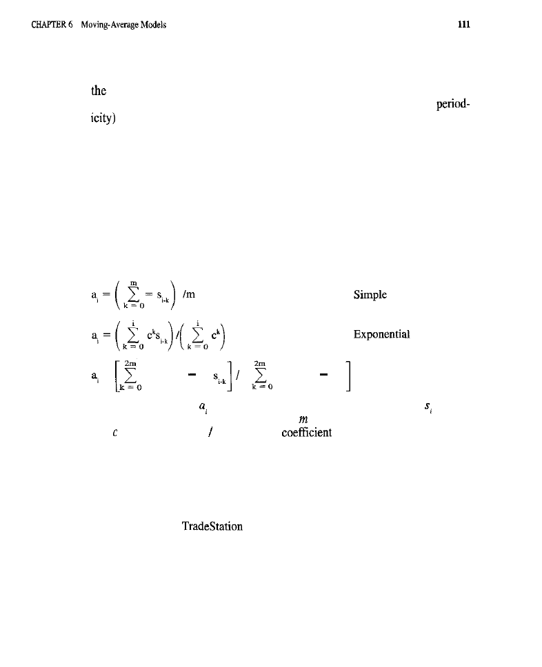
eliminated by combining several moving averages to create a band-pass filter.
Band-pass filters can have effectively zero lag for signals with periodicities near
center of the pass-band; the smoothed signal can be coincident with the origi-
nal, noisy signal when there is cyclic activity and when the frequency (or
of the cyclic activity is close to the frequency maximally passed by the filter.
T Y P E S O F M O V I N G A V E R A G E S
All moving averages, from the simple to the complex, smooth time
series data
by
some kind of averaging process. They differ in how they weigh the sample points
that are averaged and in how well they adapt to changing conditions. The differ-
ences between moving averages arose from efforts to reduce lag and increase
responsiveness. The most popular moving averages (equations
below) are the sim-
ple moving average,
the
exponential moving average, and the front-weighted tri-
angular moving average. Less popular is Chande’s
adaptive moving average
(1992).
=
(2m + 1 k)
(
(2m + 1 k) Front-weighted triangular
In the equations, represents the moving average at the
i-th
bar, the i-th
bar or data point of the original time series,
the period of the moving average,
and (normally set to 2 (m + I)) is a
that determines the effective
period for the exponential moving average. The equations show that the moving
averages differ in how the data points are weighted. In a simple moving average,
all data points receive equal weight or emphasis. Exponential moving averages
give more weight to recent points, with the weights decreasing “exponentially”
with distance into the past. The front-weighted triangular moving average
weighs the more recent points more heavily, but the weights decline in a linear
fashion with time;
calls this a “weighted moving average,” a pop-
ular misnomer.
Adaptive moving averages were developed to obtain a speedier response. The
goal was to have the moving average adapt to current market behavior, much as
Dolby noise reduction adapts to the level of sound in an audio signal: Smoothing
increases when the market exhibits mostly noise and little movement (more noise
attenuation during quiet periods), and smoothing declines (response quickens) dur-
ing periods of more significant market activity (less noise suppression during loud

passages). There are several adaptive moving averages. One that seems to work
well was developed by Mark
Another was
(Variable Index Dynamic Moving Average) developed by Chande.
A recursive algorithm for the exponential moving average is as follows: For
each bar, a coefficient
that determines the effective length
of the moving
average is multiplied by the bar now being brought into the average and, to the
result, is added
1.0
c multiplied by the existing value of the moving average,
yielding an updated value. The coefficient is set to
+ m)
where is the
desired length or period. Chande (1992) modified this algorithm by changing the
coefficient (c) from a fixed number to a number determined by current market
volatility, the market’s “loudness,” as measured by the standard deviation of the
prices over some number of past bars. Because the standard deviation can vary
greatly between markets, and the measure of volatility needs to be relative,
Chande divided the observed standard deviation on any
by the average of the
standard deviations over all bars on the S&P 500. For each bar, he recomputed the
coefficient in the recursive algorithm as 2.0
(1.0
+
multiplied by the rela-
tive volatility, thus creating a moving average with a length that dynamically
responds to changes in market activity.
We implemented an adaptive moving average based on VIDYA that does not
require a fixed adjustment (in the form of an average of the standard deviations over
all bars) to the standard deviation. Because markets can change dramatically in their
average volatility over time, and do so in a way that is irrelevant to the adaptation of
the moving average, a fixed normalization did not seem sound. We replaced the stan-
dard deviation divided by the normalizing factor (used by Chande) with a ratio of
measures of volatility: one shorter term and one longer term. The relative
volatility required for adjusting c, and hence the period of the adaptive moving aver-
age, was obtained by dividing the shorter term volatility measure by the longer term
volatility measure. The volatility measures were exponential moving averages of the
squared differences between successive data points. The shorter moving average of
squared deviations was set to a period of an adjustable parameter, while the peri-
od of the longer moving average was set top multiplied by four. If the longer term
volatility is equal to the most recent volatility (i.e., if their ratio is
then the adap-
tive moving average behaves identically to a standard exponential moving average
with period m; however, the effective period of the exponential moving average is
monotonically reduced with an increasing ratio of short-term to long-term volatility,
and increased with a declining ratio of short-term to long-term volatility.
TYPES OF MOVING AVERAGE ENTRY MODELS
A moving
entry model generates entries using simple relationships
between a moving average and price, or between one moving average and another.
Trend-following and
models exist. The most popular models follow

the trend and lag the market. Conversely, countertrend moving average models
anticipate reversals and lead, or coincide with, the market. This is not to imply that
countertrend systems trade better than trend-following ones. Consistently entering
trends, even if late in their course, may be a more reliable way to make money than
anticipating reversals that
sometimes occur when expected. Because of the
need for a standard exit, and because no serious trader would trade without the pro-
tection of money management stops, simple moving average models that are
always in the market are not tested. This kind of moving average reversal model
will, however, be fairly well-approximated when fast moving averages are used,
causing reversal signals to occur before the standard exit closes out the trades.
Trend-following entries may be generated in many ways using moving aver-
ages. One simple model is the
The trader buys when
prices cross above the moving average and sells when they cross below. Instead of
waiting for the raw prices to cross a moving average, the trader can wait for a faster
moving average to cross a slower one: A buy signal occurs when the faster moving
average crosses above the slower moving average, and a sell is signalled when the
crossover is in the other direction. Smoothing the raw price series with a fast mov-
ing average reduces spurious crossovers and, consequently, minimizes whipsaws.
Moving averages can also be used to generate
entries. Stock prices
often react to a moving average line as they would to the forces of support or resis-
tance; this forms the basis of one
entry model. The rules are to buy when
prices touch or penetrate the moving average from above, and to sell when
is from below. Prices should bounce off the moving average, reversing direction.
Countertrend entries can also be achieved by responding in a
to a
standard crossover: A long position is taken in response to prices crossing below a
moving average, and a short position taken when prices cross above. Being contrary-
doing
opposite of what seems
works when trading: It can be prof-
itable to sell into demand and buy when prices drop in the face of heavy selling. Since
moving averages lag the market, by the time a traditional buy signal is given, the mar-
ket may just about to reverse direction, making it time to sell, and vice versa.
Using a moving average in a
model based on support and resis-
tance is not original. Alexander (1993) discussed
to moving average
port after a crossover as one way to set up an entry.
(1998) discussion of a
two parameter moving average model, which uses the idea of support and resistance
to trade mutual funds, is also relevant. Finally, Sweeney (1998) described the use of
an end-of-day moving average to define
levels of support and resistance.
CHARACTERISTICS OF MOVING AVERAGE
ENTRIES
A trend-following moving average entry is like a breakout: Intuitively appealing
and certain to get the trader aboard any major trend: it is also a traditional, readily

available approach that is easy to understand and implement, even in a spreadsheet.
However, as with most trend-following methods, moving averages lag the market,
i.e., the trader is late entering into any move. Faster moving averages can reduce lag
or delay, but at the expense of more numerous whipsaws.
A countertrend moving average entry gets one into the market when others
are getting out, before a new trend begins. This means better fills, better entry
prices, and greater potential profits. Lag is not an issue in countertrend systems.
The danger, however, is entering too early, before the market slows down and turns
around. When trading a countertrend model, a good risk-limiting exit strategy is
essential; one cannot wait for the system to generate an entry in the opposite direc-
tion. Some countertrend models have strong logical appeal, such as when they
employ the concept of support and resistance.
O R D E R S U S E D T O E F F E C T E N T R I E S
Entries based on moving averages may be effected with stops, limits, or market
orders, While a particular entry order may work especially well with a particular
model, any entry may be used with any model. Sometimes the entry order can
form part of the entry signal or model. A basic crossover system can use a stop
order priced at tomorrow’s expected moving average
To avoid
whipsaws, only a buy stop or a sell stop (not both) is issued for the next day. If the
close is above, a sell stop is posted; if below, a buy stop.
Entry orders have their own advantages and disadvantages. A market order
will never miss a signalled entry. A stop order will never miss a significant trend
(in a trend-following model), and entry will never occur without
by
movement in favor of the trade; the disadvantages are greater slippage and less
favorable entry prices. A limit order will get the best price and minimize transac-
tion costs, but important trends may be missed while waiting for a
to
the limit price. In countertrend models, a limit order may occasionally worsen the
entry price: The entry order may be filled at the limit price, rather than at a price
determined by the negative slippage that sometimes occurs when the market
moves against the trade at the time of entry!
T E S T M E T H O D O L O G Y
In all tests that follow, the standard portfolio is used. The number of contracts to
buy or sell on entry, in any market, at any time, was chosen to approximate the dol-
lar volatility of two S&P 500 contracts at the end of 1998. Exits are the standard
ones. All tests are performed using the C-Trader toolkit. The portfolios, exit strate-
gies, and test platform are identical to those used previously, making all results
comparable. The tests are divided into trend-following and
ones.
They were run using a script containing instructions to set parameters, run

CHAPTER 6
Moving-Average Models
and generate output for each combination of moving average type,
model, and entry order.
The code below is more complex than for breakouts: Instead of a different
routine for each combination of moving average, entry rule, and trading order,
there is one larger routine in which parameters control the selection of system ele-
ments. This technique is required when systems are genetically evolved. Although
no genetics are used here, such algorithms are employed in later chapters. This
code uses parameters to control model elements, making it easier to handle all the
combinations tested in a clean, systematic way.
clearer
period for faster moving average
period for slower
average
type
entry
type
moving average
type
entry
maximum holding period
profit target in volatility units
stop loss in volatility units

116
skip invalid parameter combinations
1,
return;
perform whole-series computations using vector routines
hi,
for exit
(
select type of
average
case 1:
simple moving averages
case 2:
averages
3:
front-weighted triangular moving averages
4:
moving averages
average
avoid placing orders
possibly limit-locked days
if
lo
continue;
generate entry
stop prices and limit prices
the specified moving average entry
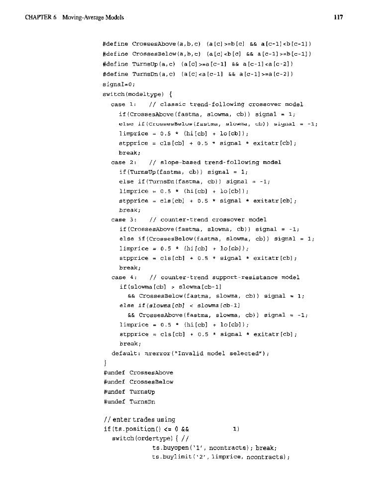
specified order type
signal ==
(
select desired order type
case 1:
case 2:
break;

The code contains three segments. The first segment calculates moving aver-
ages. A parameter
selects the kind of average: 1 = simple; 2 = expo-
nential: 3 = front-weighted triangular; and 4 = the modified VIDYA. Even if the
model requires only one moving average, two of the same type are computed, this
allows the selection of the moving average to be independent of model selection.
The average
range is also computed and is required for setting stop-losses and
profit targets in the standard exit strategy. Two additional parameters,
and
specify the period of the faster and the slower moving averages,
respectively. The moving averages are saved in the
and
The next block uses the selected model to generate entry signals, stop prices,
and limit prices. First, simple relationships
and
are defined. Depending on
modeltype,
one of four mov-
ing average models then generates the signals: = the classic, trend-following dual
moving average crossover; 2 a slope-based trend-following model; 3 = a
crossover model; and 4 = a
support/resistance model. In the
classic, trend-following dual moving average crossover, the trader goes long if a
faster moving average of the closing price crosses above a slower moving average,
and goes short if the faster moving average crosses below the slower one. As a spe-
cial case, this model contains the classic crossover that compares prices to a mov-
ing average. The special case is achieved when the period of the shorter moving
average is set to 1, causing that moving average to decay to the original series,
the closing prices. With a slope-based trend-following model, the trader buys when
the moving average was decreasing on previous bars but increases on the current
bar (slope turns up), and sells when the opposite occurs. This model requires only
the fast moving average. The countertrend model is the opposite of the classic
trend-following crossover: The trader buys when the shorter moving average (or the
price itself) crosses below the longer moving average, and sells when it crosses
above. This model is the
delight: Doing exactly the opposite of the
trend-followers. Last is a crude countertrend support/resistance model in which
prices are expected to bounce off the moving average, as if off a line of support or
resistance. The rules are almost identical to the countertrend crossover model,
except that the slower moving average must be moving in the direction of the entry:
If the slower moving average is trending upward, and prices (or the faster moving
average) move from above that slower moving average into or below it, the trader
buys; conversely, if prices (or the faster moving average) are currently below a
downward trending slower moving average, and prices bump into or penetrate that
moving average from below, then the trader sells. The additional trend rule prevents
an immediate reversal of position after contact or penetration. Without the trend
rule, a quick penetration followed by a reversal would trigger two entries: The
would be the desired countertrend entry, occurring when the prices penetrate the
moving average, and the second entry (in the opposite direction) would occur as the
prices bounce back, again crossing the moving average. The trend check only
allows entries to be taken in one direction at a time. A penetration, followed by a
bounce in an up-trending market, will take the long entry; a penetration and rever-
sal in a down-trending market will result in a short entry.
In the last block of code, the entry order to be posted is determined by the
parameter: 1 = market at open; 2 = limit; 3 = stop. Whether a buy or
sell is posted, or no order at all, is determined by whether any signal was generat-
ed in the previous block of code; a variable called signal carries this information: 1
= buy; 1 = sell (go short); 0 = do nothing. The limit price
is com-
puted as the sum of today’s high and low prices divided by two. Because many of
the models have no natural price for setting a stop, a standard stop was used. The
standard entry stop price
is obtained by taking the closing price of the
previous bar and adding (if a long position is signalled) or subtracting (if a short is
the
average true range multiplied by 0.50; the market must move
at least one-half of its typical daily range, in the direction of the desired entry, for
the entry to occur. This type of stop order adds a breakout test to the moving aver-
age system: Once a signal is given, the market must move a certain amount in the
direction of the trade to trigger an entry. Because of the large number of tests, sta-
tistical
were not reported unless something notable occurred.
TESTS
TREND-FOLLOWING MODELS
The group of tests presented here involve moving averages as trend-followers. The
models vary in the kinds of moving average, the rules that generate signals, and
the orders posted to effect entry. The moving averages tested include the simple,
the exponential, the front-weighted triangular, and a modification of VIDYA. Both
single and dual moving average crossovers, and models that use slope (rather than
crossover) to determine entry, are examined. Entry orders are market-at-open,
stop, and limit.
Tests 1 through 12 were of the crossover models, Optimization was per-
formed by stepping the length of the shorter moving average from 1 to 5, in incre-
ments of 1, and the longer moving average from 5 to 50, in increments of 5. Only
cases in which the longer moving average was strictly longer than the shorter mov-
ing average were examined. Brute force optimization was used, controlled by the
testing script. The parameters were chosen to maximize the risk-to-reward ratio or,
equivalently, minimize the probability (based on a t-test of daily returns) that any
profitable performance was due to chance. In Tests 13
24 (the slope mod-
els), brute-force optimization was performed by stepping the length of the first
and, in this case, only moving average from 3 to 40, in increments of 1. As in Tests
1
12, the risk-to-reward ratio was maximized. Optimization was only car-
ried out on in-sample data.
Tables 6-l and 6-2 show, for each of the 24 tests, the specific commodities that
the model traded profitably and those that lost, for the in-sample (Table 1) and
of-sample (Table 6-2) runs. The
column represents the market being studied;
the first row identifies the test. The data provides relatively detailed information
about which markets were and were not profitable when traded by each of the mod-
els: One dash
indicates a moderate loss per trade, i.e., $2,000 to $4,000, two
dashes -) represent a large loss per trade, i.e., $4,000 or more; one plus sign
means a moderate profit per trade, i.e., $1,000 to $2,000; two pluses
indicates
a large gain per trade, i.e., $2,000 or more; a blank cell means that the loss was
between $0 and $1,999 or the profit was between $0 and $1,000 per trade.
Table 6-3 shows, for the entire portfolio, the return-on-account
and
average dollar-per-trade
broken down by the moving average, model,
entry order, and sample. The last two columns on the right, and the last four rows
of numbers on the bottom, are averages. The numbers at the bottom have been
averaged over all combinations of moving average type and model. The numbers
at the right are averaged over order type.
None of the trend-following moving average models was profitable on a port-
folio basis. More detailed examination reveals that for the crossover models the
limit order resulted in a dramatic benefit on the in-sample data. When compared
with an entry at open or on a stop, the limit cut the loss of the average trade almost
in half. Out-of-sample, the improvement was not as dramatic, but still significant.
The return-on-account showed a similar pattern: The least loss was with the limit
order. For slope models, the limit order worked best out-of-sample in terms of dol-
lars per trade. The return-on-account was slightly better with a stop (due to distor-
tions in the
ROA%
numbers when evaluating losing systems), and worse for entry
at open. In-sample, the stop order performed best, but only by a trivial amount.

In-Sample Performance Broken Down by Test and Market
In-sample, the simple moving average provided the best results in average
dollars-per-trade. The worst results were for the adaptive moving average. The
other two moving averages fell in-between, with the exponential better in the
crossover models, and the front-weighted triangular in the slope models. Of the
crossover models, the
ROA%
was also the best for the simple moving average.
Overall, the crossover models did as well or better than the slope models, possi-
bly because of a faster response to market action in the former. Out-of-sample,
the simple moving average was
clear winner for the crossover models, while
the front-weighted triangular was the best for the slope models. In terms of the

T A B L E 6 - 2
Out-of-Sample Performance Broken Down by Test and Market
ROA%,
the exponential moving average appeared the best for the crossover
models, with the front-weighted triangular still the best for the slope models.
When looking at individual tests, the particular combination of a
weighted triangular moving average, the slope model, and entry on stop (Test 21)
produced the best out-of-sample performance of all the systems tested. The
sample results for the front-weighted triangular slope models seemed to be better
across all order types. There apparently were
strong interactions between the
various factors across all tests, e.g., for the crossover model on the in-sample data,
entry at the open was consistently close to the worst, entry on stop was somewhere
in between, and entry on limit was always best, regardless of the moving average
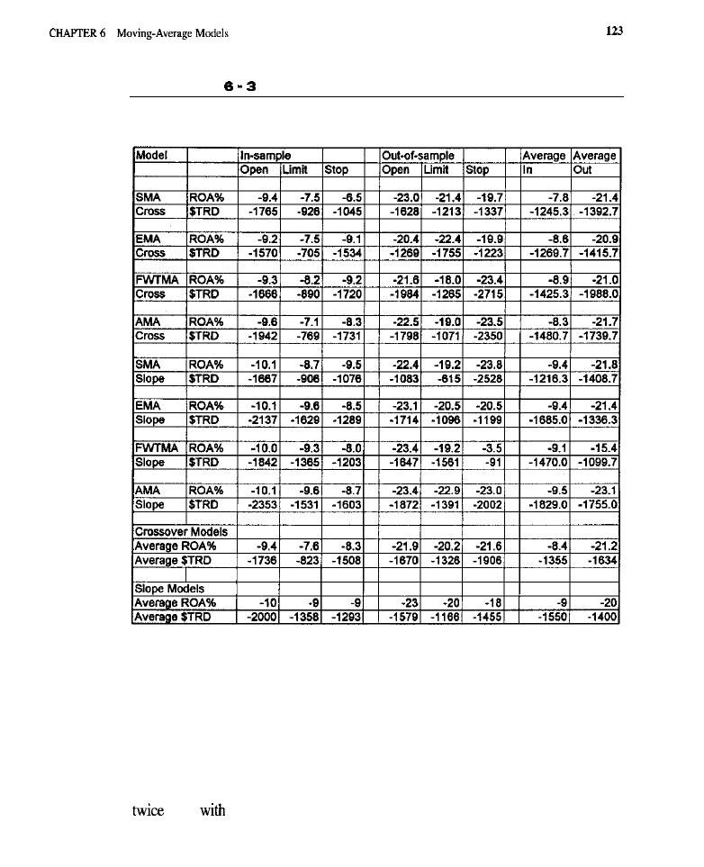
T A B L E
Performance of Trend-Following Moving Average Entry Models
Broken Down by Order, Moving Average Type, Model, and Sample
used. Out-of-sample, the findings were much more mixed: With the simple moving
average, the pattern was similar to that for the in-sample period; however, with the
exponential moving average, the limit performed worst, the stop best, and the open
not far behind. Out-of-sample, with the front-weighted triangular average, the stop
performed by far the worst, with the limit back to the best performer. These results
indicate interaction between the moving average, entry order, and time.
The slope model, in-sample, had the entry at open always performing worst;
however, although the results were often quite close, the limit and stop orders were
seen
the limit being favored (simple moving average and adjusted moving

average),
twice with the stop being favored (exponential moving average and
front-weighted triangular moving average). As before, great variation was seen out-
of-sample.
For the simple moving average, the limit order performed best and the stop
worst. The more typical pattern was seen for the exponential moving average: The
entry at open performed worst, the limit best, and the stop was on the heels of the
limit. As already stated, the front-weighted triangular moving average performed
unusually when combined with the stop order. The limit was best for the
adaptive moving average, the stop was worst, and the open was slightly better
albeit
close to the stop.
As a whole,
models lost on most markets. Only the
and Pork
Bellies were profitable both in- and out-of-sample; no other markets were profitable
in-sample. Out-of-sample, some profits were observed for Heating Oil, Unleaded
Gasoline, Palladium, Live Hogs, Soybean Meal, Wheat, and Coffee. The strong out-
of-sample profit for Coffee can probably be explained by the major run-up during the
drought around that time. On an individual model-order basis, many highly profitable
combinations could be found for Live Hogs,
Pork Bellies, Coffee, and
Lumber. No combinations were profitable in either sample for Oats.
In terms of equity averaged over all averages and models, entry at the open
performed, by far, the worst. Entry on limit or stop produced results that were
close, with the limit doing somewhat better, especially early in the test period. It
should be noted that, with the equity curves of losing systems, a distortion takes
place in their reflection of how well a system trades. (In our analyses of these los-
ing systems, we focused, therefore, on the average return-per-trade, rather than on
risk-reward ratios, return-on-account, or overall net profits.) The distortion
involves the number of trades taken: A losing system that takes fewer trades will
appear to be better than a losing system that takes more trades, even if the better
appearing system takes trades that lose more on a per-trade basis. The very heavy
losses with entry at open may not be a reflection of the bad quality of this order;
it may simply be reflecting that more trades were taken with an entry at the open
than when a stop or limit order was used.
Figure 6-l presents the equity curves for all eight model and moving average
combinations. The equity curves were averaged across order type. Figure 6-l pro-
vides a useful understanding of how the systems interact with time. Most of the sys-
tems had their heaviest losses between late 1988 and early 1995. The best
performance occurred before 1988, with the performance in the most recent period
being intermediate. In Curve 3, the simple moving average crossover model was the
most outstanding: This pattern was greatly exaggerated, making the equity curve
appear very distinct; it actually showed a profit in the early period, a heavier rela-
tive loss in the middle period, and
off (with a potential return to flat or prof-
itable behavior) toward the end of the third period. Finally, it is dramatically evident
that the crossover systems (Curves 1 through 4) lost much less heavily than the
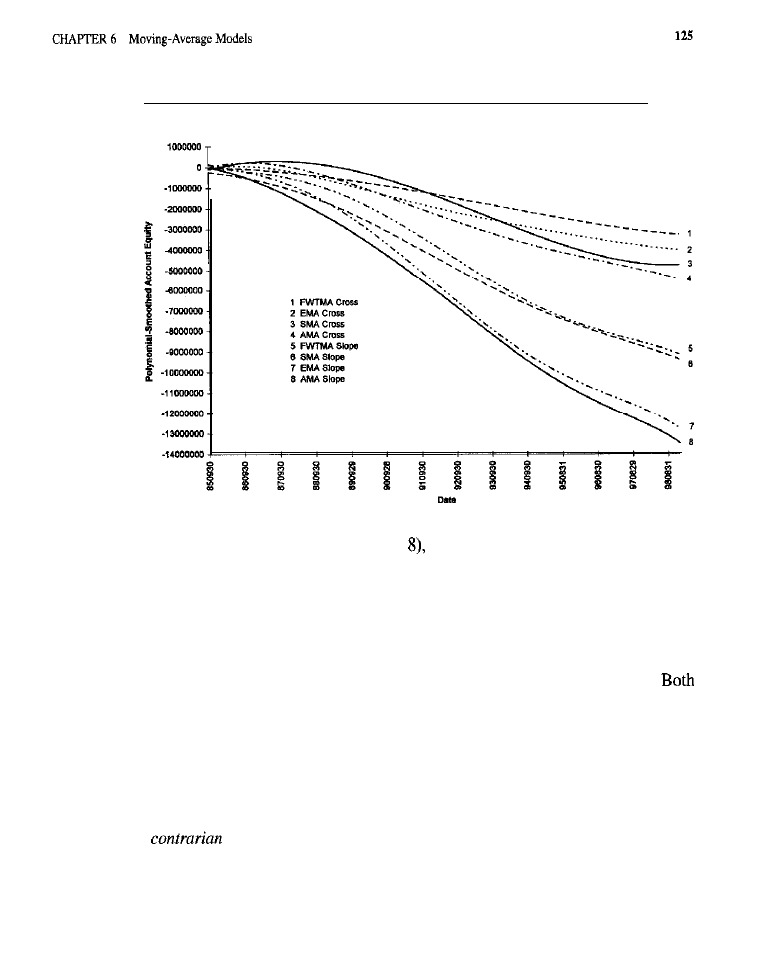
F I G U R E 6 - 1
Equity Curves for Each Model and Moving Average Combination
slope-based models (Curves 5 through
although this reflects a larger number of
trades, not greater losses on a per trade basis.
TESTS OF COUNTER-TREND MODELS
As with trend-following models, countertrend models vary in the moving averages
used, the rules that generate signals, and the orders posted to effect entry. The
same moving averages used in the trend-following models are studied here.
single and dual moving average models are examined. Entry orders studied are the
market-at-open, stop, and limit.
Tests 25 through 36 evaluate the standard moving average crossover model
turned upside-down. As before, entry signals occur when prices cross the average,
or when a shorter average crosses a longer one. In traditional trend-following
crossover models, the trader buys when the price (or a shorter moving average)
crosses above a longer moving average, and sells when it crosses below. In the
crossover model, the trader sells when prices cross above, and buys
when prices cross below. In these tests, brute force optimization was performed on
the in-sample data by stepping the length of the shorter moving average from 1 to
7, in increments of 1; the longer moving average was stepped from 5 to 50, in

increments of 5. Only cases where the longer moving average was longer than the
shorter moving average were considered. The parameters minimized the probabil-
ity that any observed profitable performance was due to chance. The model was
run on the out-of-sample data using the best parameter set found in-sample.
In tests of the support/resistance model (37 through
the trader buys when
prices bounce off a moving average from above, and sells when they hit a moving
average from below. In this way, the moving average serves as a line of support or
resistance where prices tend to reverse. The rules are almost the same as for Tests 25
through 36, except that not every penetration of a moving average results in an entry.
If prices are above the moving average and penetrate it, a buy is generated; howev-
er, when prices bounce back up through the moving average, the second crossover
is not allowed to trigger a sell. If prices arc below the moving average and rise into
it, a sell is triggered, no buy is triggered when the prices bounce back down. This
behavior is achieved by adding one element to the
crossover model: A sig-
nal is generated only if it is in the direction of the slope of the slower moving aver-
age. Performance was brute force optimized on the in-sample data by stepping the
length of the shorter moving average from 1 to in increments of 1, and the longer
moving average from 5 to 50, in increments of 5. A moving average length of 1
caused the shorter moving average to become equivalent to the prices; therefore, in
the optimization, the model in which prices were compared to the moving average
was tested, as was the model in which one moving average was compared to
er. Only cases where the longer moving average was strictly longer than the shorter
moving average were examined. The parameters were chosen to minimize the prob-
ability that any profitable performance was due to chance. The model was then run
on the out-of-sample data using the best parameter set found in-sample.
Tables 6-4 and 6-5 show, for Tests 25 through 48, the commodities that the
model traded profitably and those that lost, in-sample (Table 6-4) and out-of-sam-
ple (Table 6-S). The plus and dash symbols may be interpreted in the same man-
ner as for Tables 6-1 and 6-2.
Table 6-6 provides the results broken down by the moving average, model,
order, and sample. The last two columns on the right, and the last four rows of
numbers on the bottom, are averages. The numbers at the bottom were averaged
over all combinations of moving average type and model. The numbers at the right
were averaged over order type.
Overall, the best models in-sample were the simple moving average sup-
port/resistance and the front-weighted triangular average support/resistance. The
simple average support/resistance with a stop order was unique in that it showed
small profits in both samples: an average trade of $227 and a 4.2%
account in-sample, $482 per trade and a 14.8% return-on-account out-of-sample.
The front-weighted triangular average with the stop was profitable in-sample, but
lost heavily out-of-sample. Both models, especially when combined with a stop,
had relatively few trades: consequently, the results are less statistically stable.

T A B L E 6 - 4
In-Sample Performance Broken Down by Test and Market
Overall, in-sample, the stop order was best for
and for sup-
port/resistance models, in which the stop led to an average profitable result, and
the other two orders led to losses; the market-at-open was the worst order.
sample, the market-at-open order was still, overall, worst for both the contrarian
crossover and the support/resistance models;
limit was best. There were much
greater losses out-of-sample than in-sample for both models.
The
models
less well than
trend-following ones;
however, there were outstanding combinations of counter-trend model, average
and entry order that performed far better than most other combinations tested.
On the basis of the moving average and breakout results, it appears that,
with trend-following models, a limit order almost always helps performance; for
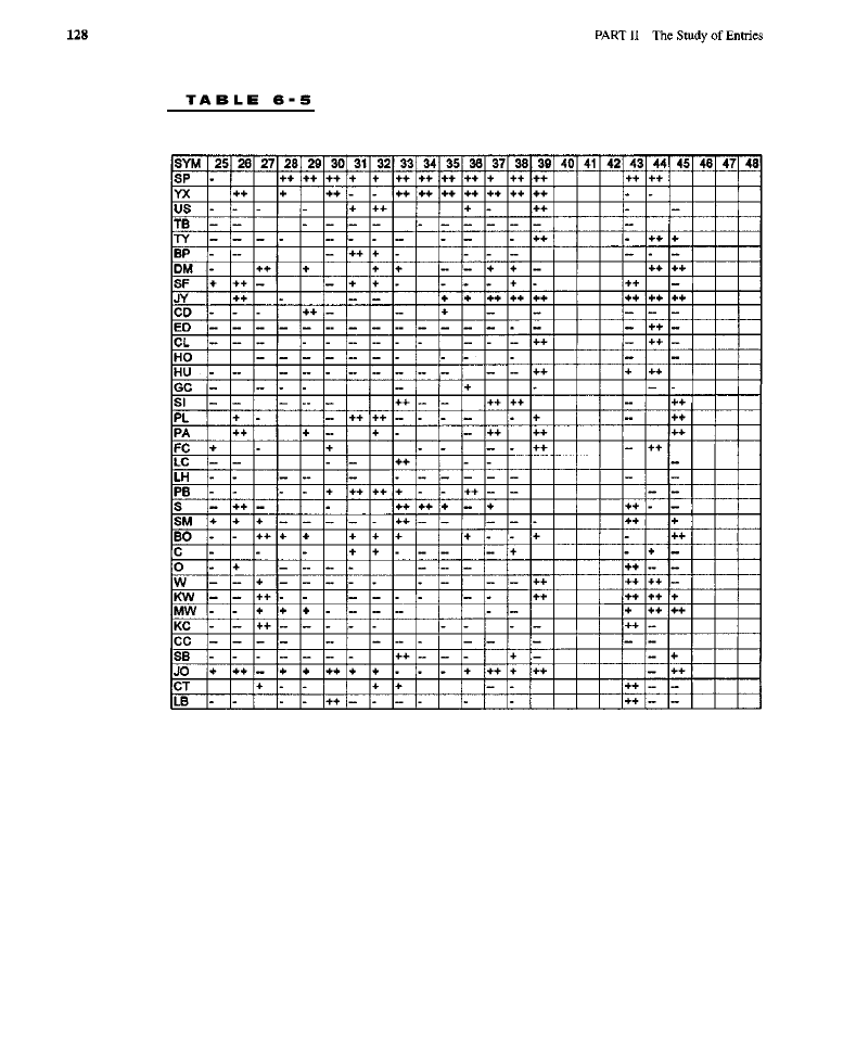
Out-of-Sample Performance Broken Down by Test and Market
countertrend models, a stop sometimes provides an extra edge. This tendency
might result from trend-following models already having a trend detection ele-
ment: Adding another detection or verification element (such as an entry on a
stop) is redundant, offering no significant benefit; however, the addition of a limit
order provides a countertrend element and a cheaper entry, thus enhancing per-
formance. With countertrend models, the addition of a trend verification element
provides something new to the system and, therefore, improves the results.
Sometimes it is so beneficial that it compensates for the less favorable entry
prices that normally occur when using stops.
On a market-by-market basis, model-order combinations that were strongly
profitable in both samples could be found for T-Bonds, JO-Year Notes, Japanese
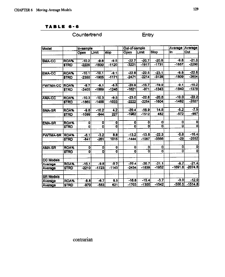
Summary of
Moving Average
Models Broken
Down by Order, Moving Average Type, Model, and Sample
Yen, Deutschemark, Swiss Franc, Light Crude, Unleaded Gasoline, Coffee,
Orange Juice, and Pork Bellies.
Figure 6-2 depicts equity curves broken down by model and moving average
combination; equity was averaged over order type. The best two models were the
front-weighted triangular average support/resistance and the simple average sup-
port/resistance. The best support/resistance models performed remarkably better
than any of the
crossover models. There were three eras of distinct
behavior: the beginning of the sample until October 1987, October 1987 until June
1991, and June 1991 through December 1998, the end of the sample. The worst
performance was in the last period.
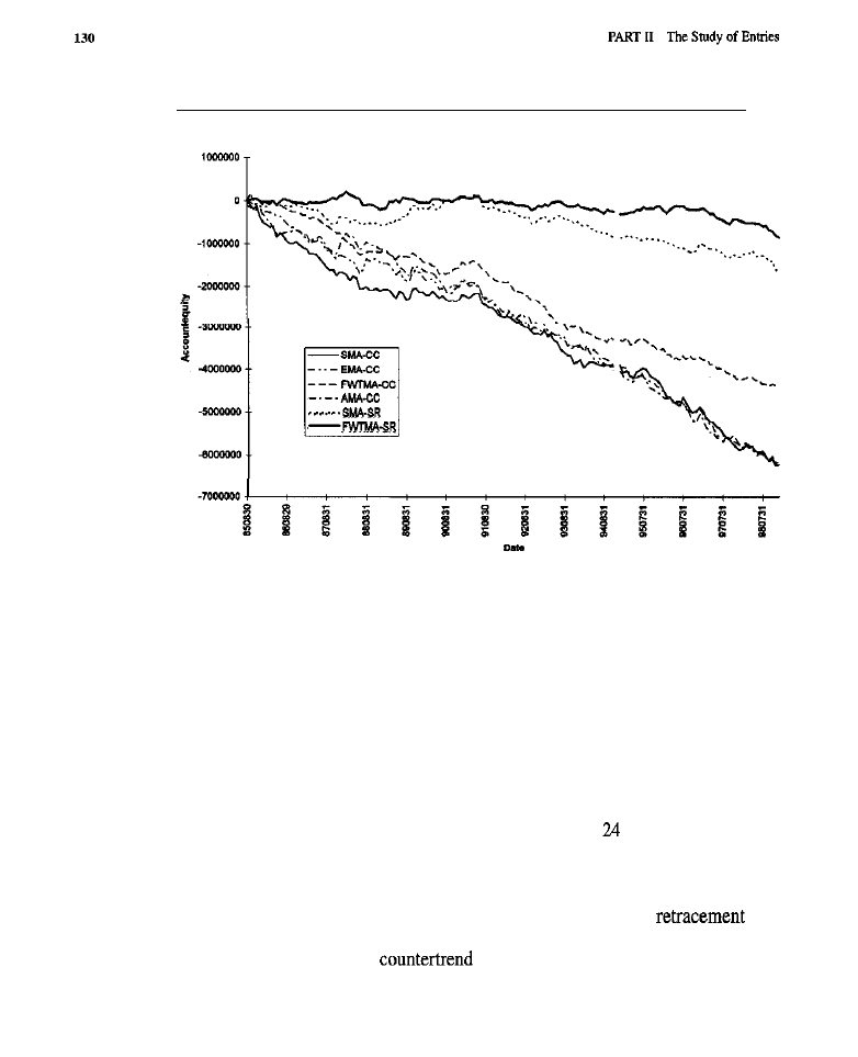
F I G U R E 6 - P
Equity Curves by Model and Moving Average Combination
On the basis of the equity curves in Figure 6-2, as well as others not
shown, it is evident that the countertrend models were better in the past, while
the trend-following models performed better in recent times. In-sample, the
stop order was best for every model-average combination, and, out-of-sample,
for three of the six (two combinations had no trades so were not considered);
entry at the open was worst in all but two cases. The stop was generally supe-
rior to the limit order, in-sample; out-of-sample, the limit was only marginally
better than the stop.
CONCLUSION
In general, the trend-following models in Tests 1 through
performed better than
the countertrend models in Tests 25 through 48, with a number of exceptions dis-
cussed above.
The best models apparently are those that combine both countertrend and
trend-following elements. For example, attempting to buy on a
with
a limit, after a moving average crossover or breakout, provides better results than
other combinations. In the
moving average models, those that have

a trend-following element (e.g.. a stop) perform better.
countertrend models
and pure trend-following models do not fare as well. Moreover, adding a
following
to an already trend-following system does not seem beneficial,
but may instead increase entry cost. Traders should try combining one of these
countertrend models with something like the ADX trend filter. Although the ADX
filter may not have helped breakouts (because,
the stop, it represents anoth-
er trend-following element added to an already trend-following model), in a
countertrend model such an element may provide an edge. As true with break
outs, the limit order performed best, except when the stop was beneficial due to
its trend filtering characteristics,
The results suggest certain generalizations. Sometimes a stop can provide
enough benefit to overcome the extra transaction costs associated with it, although
a limit order generally performs best because of its ability to reduce costs. While
such a generalization might help guide a trader’s choices, one has to watch for
potential interactions within the moving average type-model-order combinations
that may cause these generalizations to fail. The variables interact: Although each
variable may have its own characteristic effect, when put in combination with
other variables, these effects may not maintain their integrity, but may change due
to the coupling; this is demonstrated in the tests above. Sometimes variables do
maintain their integrity, but not always.
WHAT HAVE WE LEARNED?
. When designing an entry model, try to effectively combine a
element with a trend-following one. This may be done in any number of
ways, e.g., buy on a short-term countertrend move when a longer-term
trend is in progress; look for a breakout when a countertrend move is in
progress; or apply a trend-following filter to a countertrend model.
n
If possible, use orders that reduce transaction costs, e.g., a limit order for
entry. But do not be rigid: Certain systems might perform better using
another kind of order, e.g., if a trend-following element is needed, a stop
might be advisable.
n
Expect surprises. For the slope-based models, we thought the adaptive,
moving average, with its faster response, would provide the best perfor-
mance; in fact, it provided one of the worst.
. Even though traditional indicators, used in standard ways, usually fail (as
do such time-honored systems as volatility breakouts), classical concepts
like
may not fail; they may actually be quite useful. In
breakouts, models based on the notion of support/resistance held up bet-
ter than did, e.g., volatility breakouts. Likewise, moving average models

using the concept of support/resistance did better than others. The sup-
port/resistance implementation was rudimentary, yet, in the best combina-
tion, it was one of the best performers; perhaps a more sophisticated
version could provide a larger number of more profitable trades.
Although support/resistance seems to be an important concept, further
research on it will not be easy. There are many variations to consider
when defining levels of support and resistance. Determining those levels
can be quite challenging, especially when doing so mechanically.

C H A P T E R 7
Oscillator-Based Entries
have been popular among technical traders for many years. Articles
that describe oscillators appear quite frequently in such magazines as Technical
Analysis of Stocks and Commodities
and
Futures.
The
subject
is also covered in
many
books
on uading.
Most widely used, in both their classic forms and variations, are Appel’s
(1990) Moving Average Convergence Divergence (MACD) oscillator and
Histogram (MACD-H). Also highly popular are Lane’s Stochastic, and Williams’s
Relative Strength Index (RSI). Many variations on these oscillators have also
appeared in the literature. Other oscillators include Lambert’s Commodities
Channel Index (CCI), the Random Walk Index (which might be considered an
oscillator), and
Goedde’s (1997)
Regression Channel Oscillator. In this chapter,
the primary focus is on the three most popular oscillators: the MACD,
and the
W H A T I S A N O S C I L L A T O R ?
An
oscillator
is an indicator that is usually computed from prices and that tends to
cycle or “oscillate” (hence the name) within a fixed or fairly limited range.
Oscillators are characterized by the normalization of range and the elimination of
long-term trends or price levels. Oscillators extract information about such tran-
sient phenomena as momentum and overextension.
Momentum is when prices
move strongly in a given direction.
Overextension
occurs when prices become
excessively high or low (“overbought” or “oversold”) and are ready to snap back
to more reasonable values.
KINDS OF OSCILLATORS
There are two main forms of oscillators. Linear band-pass filters are one form of
oscillator. They may be analyzed for frequency (periodicity) and phase response.
The MACD and MACD-H are of this class. Another form of oscillator places
some aspect of price behavior into a normalized scale (the
and
belong to this class); unlike the first category, these oscillators are not linear
filters with clearly defined phase and frequency behavior. Both types of oscillators
highlight momentum and cyclical movement, while downplaying trends and elim-
inating long-term offsets: i.e., they both produce plots that tend to oscillate.
The
Average Convergence Divergence Oscillator, or
(and
MACD-Histogram), operates as a crude band-pass filter,
both slow
trends and offsets, as well as high-frequency jitter or noise. It does this while pass-
ing through cyclic activity or waves that fall near the center of the pass-band. The
MACD smooths data, as does a moving
but it also removes some of the
trend, highlighting cycles and sometimes moving in coincidence with the market,
i.e., without lag. Ehlers (1989) is a good source of information on this oscillator.
The MACD is computed by subtracting a longer moving average from a
shorter moving average. It may be implemented using any kind of averages or low-
pass filters (the classic MACD uses exponential moving averages). A number of
variations on the MACD use more advanced moving averages, such as the VIDYA
(discussed in the chapter on moving averages). Triangular moving averages have
also been used to implement the MACD
Along with the raw MACD, the
so-called MACD Histogram (MACD-H) is also used by many traders. This is
computed by subtracting from the MACD a moving average of the MACD. In
many cases, the moving average of the MACD is referred to as a
line.
The Stochastic oscillator is frequently referred to as an overbought/oversold
indicator. According to Lupo
“The stochastic measures the location of the
most recent market action in relation to the highest and lowest prices within the
last bars. In this sense, the Stochastic is a momentum indicator: It answers
the question of whether the market is moving to new highs or new lows or is just
meandering in the middle.
The Stochastic is actually several related indicators: Fast
Slow %K
(also known as Fast
and Slow %D. Fast
measures, as a percentage, the
location of the most recent closing price relative to the highest high and lowest low
of the last bars, where is the length or period set for the indicator. Slow
which is identical to Fast
applies a
(or
moving average to both
the numerator and denominator when computing the
value. Slow
is sim-
ply a
simple moving average of Slow
it is occasionally treated as a sig-
nal line in the same way that the moving average of the MACD is used as a signal
line for the MACD.
There have been many variations on the Stochastic reported over the years;
e.g., Blau
discussed a double-smoothing variation. The equations for the
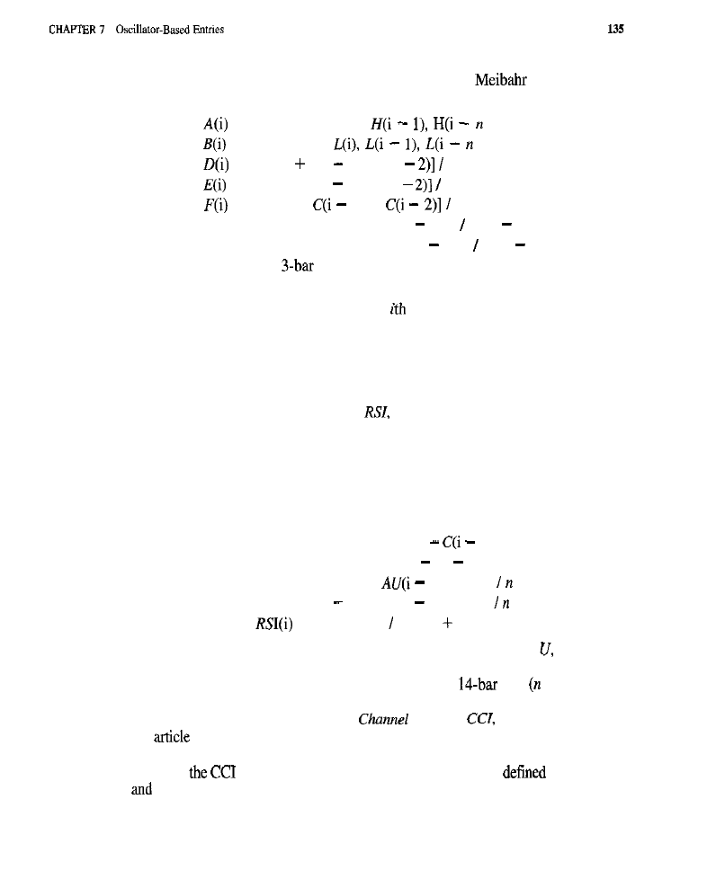
classical Lane’s Stochastic are described in an article by
(1992). A ver-
sion of those equations appears below:
= Highest of H(i),
+ 1)
= Lowest of
+ 1)
= [A(i) A(i 1) + A(i
3
= [B(i) + B(i 1) + B(i
3
= [C(i) +
1) +
3
Fast %K for ith bar = 100 * [C(i) B(i)] [A(i) B(i)]
Slow %K = Fast %D = 100 * [F(i) E(i)] [D(i) E(i)]
Slow %D =
simple moving average of Slow %K
In these equations,
i
represents the bar index, H(i) the high of the ith bar, L(i) the
low of the
ith
bar, and
C(i)
the close of the
bar. All other letters refer to derived
data series needed to compute the various Stochastic oscillators. As can be seen
from the equations, the Stochastic oscillators highlight the relative position of the
close in a range set by recent market highs and lows: High numbers (a maximum
of 100) result when the close is near the top of the range of recent price activity
and low numbers (a minimum of 0) when the close is near the bottom of the range.
The
Relative
Strength
Index,
or
is another well-known oscillator that
assesses relative movement up or down, and scales its output to a fixed range, 0 to
100. The classic RSI makes use of what is essentially an exponential moving aver-
age, separately computed for both up movement and down movement, with the
result being up movement as a percentage of total movement. One variation is to
use simple moving averages when computing the up and down movement com-
ponents. The equations for the classic RSI appear below:
C/(i) = Highest of 0, C(i)
1)
D(i)
= Highest of 0, C(i 1) C(i)
AU(i) = [(n 1) *
1) + U(i)]
AD(i)
= [(n 1) * AD(i I) +
D(i)]
= 100 *AU(i) [AU(i) AD(i)]
The indicator’s period is represented by n, upward movement by downward
movement by
D,
average upward movement by
AU,
and average downward move-
ment by
AD.
The bars are indexed by
i.
Traditionally, a
RSI = 14) would
be calculated. A good discussion of the RSI can be found in Star (1993).
Finally, there is the
Commodities
Index, or
which is discussed in
an
by Davies (1993). This oscillator is like a more statistically aware
Stochastic: Instead of placing the closing price within bands defined by recent highs
and lows,
evaluates the closing price in relation to bands
by the mean
mean deviation of recent price activity. Although not discussed further in this
chapter, the equations for this oscillator are presented below for interested readers:

136
X(i) = H(i) + L(i) + C(i)
A(i)
= Simple n-bar moving average of X(i)
D(i) = Average of
A(i)
fork
= 0 to
1
= [X(i) A(i)]
* D(i)]
In the equations for the Commodities Channel Index, X represents the so-called
median price,
A
the moving average of X,
D
the mean absolute deviations, the
period for the indicator, and the bar index.
Figure 7-l shows a bar chart for the S&P 500. Appearing on the chart are the
three most popular oscillators, along with items normally associated with them,
e.g., signal lines or slower versions of the oscillator. Also drawn on the
containing the Stochastic are the fixed thresholds of 80 and 20 often used as ref-
erence points. For the RSI, similar thresholds of 70 and 30, traditional numbers for
that oscillator, are shown. This figure illustrates how these three oscillators appear,
how they respond to prices, and what divergence (a concept discussed below)
looks like.
GENERATING ENTRIES WITH OSCILLATORS
There are many ways to generate entry signals using oscillators. In this chapter,
three are discussed.
One popular means of generating entry signals is to treat the oscillator as an
overbought/oversold indicator. A buy is signaled when the oscillator moves below
some threshold, into oversold territory, and then crosses back above that threshold.
A sell is signaled when the oscillator moves above another threshold, into over-
bought territory, and then crosses below that threshold. There are traditional
thresholds that can used for the various oscillators.
A second way oscillators are sometimes used to generate signals is with a
so-called signal line, which is usually a moving average of the oscillator.
Signals to take long or short positions are issued when the oscillator crosses
above or below (respectively) the signal line. The trader can use these signals
on their own in a reversal system or make use of additional, independent exit
rules.
Another common approach is to look for price/oscillator divergences, as
described by
(1994).
Divergence is
when prices form a lower low
while the oscillator forms a higher low (suggesting a buy), or when prices form a
higher high while the oscillator forms a lower high (suggesting a loss of momen-
tum and a possible sell). Divergence is sometimes easy to see subjectively, but
almost always difficult to detect accurately using simple roles in a program.
Generating signals mechanically for a divergence model requires algorithmic pat-
tern recognition, making the correct implementation of such models rather com-
plex and, therefore, difficult to test. Generating such signals can be done, however;
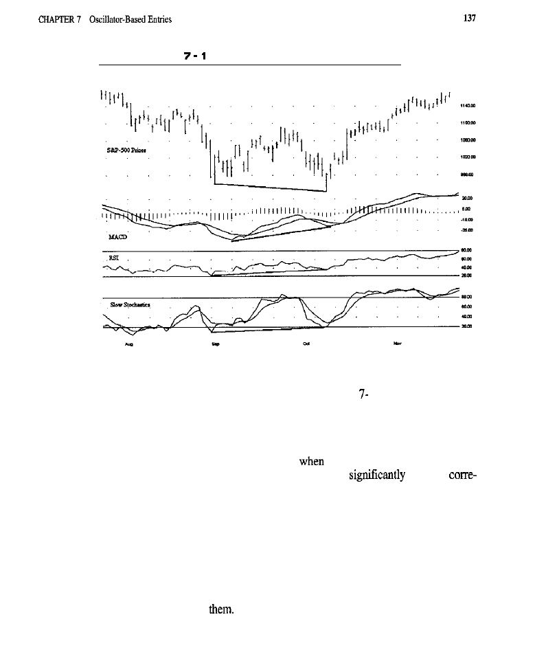
F I G U R E
Examples of Oscillators and Price-Oscillator Divergence
a good example is the “Divergengine” software distributed by Ruggiero
Associates. An example of divergence appears in Figure
1.
There are a number of issues to consider when using oscillators to generate
entries, e.g., smoothing of data and timeliness of entry. The MACD, for example,
can sometimes provide the smoothing of a moving average with the timeliness of
raw prices. The combination of timeliness and good smoothing may yield entries
that are more profitable than those obtained
using moving average entry mod-
els. The peaks and valleys in a moving average come
after the
sponding peaks and
valleys
in prices. Consequently, entries generated by looking for
these peaks and valleys, or ‘Yarning points,” are excruciatingly late. Conversely,
when cyclic activity in the market has a periodicity that matches the particular
MACD used, the peaks and valleys in the output from the MACD come at roughly
the same time as the peaks and valleys in the prices; the smoothing of a moving aver-
age is achieved without the lag of a moving average, Because the MACD smooths
the data, numerous noise-induced trades will be eliminated, as happens with moving
averages. Because the MACD can be timely, trades generated may be profitable.
In addition to the MACD, many other oscillators tend to move concurrently
with prices or even lead
For reasons to be discussed later, leading or coincident

indicators do not necessarily generate
profitable entries than such lagging indi-
cators as moving averages. Having coincident indicators does not necessarily mean
highly profitable signals. The problem is that even though some signals will occur
with precise timing, many spurious signals can result, especially in the context of
developing trends. When strong trends are present, the anticipated or coincident
reversals may simply never take place, leading to entries in the wrong direction.
Timeliness may be gained, but reliability may be lost. The question of which trade-
off provides a
profitable model-getting in reliably but late, or on time but unre-
liably-is a matter for empirical study. Such issues are present with any entry method
or pattern detection or forecasting model: The greater the delay, the more accurate
(but less useful) the detection or indication; the lesser the delay, or the further ahead
must be made, the less accurate (but more useful) the detection or indica-
tion, The logic is not unlike that of the
Uncertainty Principle.
As an example of how oscillators may be used to generate entries, consider the
Stochastic: A simple entry model might buy when this indicator drops below the tra-
ditional oversold threshold of 20 and then rises above that threshold. It might
when the indicator goes beyond the traditional overbought threshold of 80 and then
drops back under. The trader must not wait for another signal to close out the current
position, as one might do when using a moving average crossover; such a signal
might not occur for a long time, so an independent exit is essential. Traders also look
for the so-called Stochastic hook, a pattern in which the Stochastic reaches a
low,
moves up a little, and
reaches a second low at a higher level than the
A buy
signal is generated as soon as the second low becomes
A sell is generated
with the exact same pattern flipped over; i.e., a lower high follows a higher high.
As in the case of breakouts and moving averages, oscillator-generated entries
can be effected using any of several orders, such as a market at open, limit, or stop.
The advantages and disadvantages of these orders have been discussed thorough-
ly in the previous two chapters.
CHARACTERISTICS OF OSCILLATOR ENTRIES
Oscillator-based entries have the positive characteristic of leading or being coin-
cident with price activity; therefore, they lend themselves to countertrend entries
and have the potential to provide a high percentage of winning trades. Oscillators
tend to do best in cycling or nontrending (trading range) markets. When they work,
oscillators have the appeal of getting the trader in the market close to the bottom
or top, before a move has really begun. For trades that work out this way, slippage
is low or even negative, good fills are easily obtained, and the trade turns profitable
with very little adverse excursion. In such cases it becomes easy to capture a good
chunk of the move, even with a
exit strategy. It is said that the markets
trend only about 30% of the time. Our experience suggests that many markets
trend even less frequently. With appropriate filtering to prevent taking

based signals during strong trends, a great entry model could probably be devel-
oped. The kind of filtering is exactly the opposite of what was sought when test-
ing breakout systems, where it was necessary to detect the presence, rather than
the absence, of trends.
The primary weakness of simple oscillator-based entries is that they perform
poorly in sustained trends, often giving many false reversal signals. Some oscilla-
tors can easily become stuck at one of their extremes; it is not uncommon to see
the Stochastic, for instance, pegged near 100 for a long period of time in the course
of a significant market movement. Finally, most oscillator entry models do not
capture trends, unlike moving averages or breakouts, which are virtually guaran-
teed to capture any meaningful trend that comes along. Many traders say that “the
trend is your friend,” that most money is made going after the “big wave,” and that
the profits earned on such trends can make up for the frequent smaller losses of
trend-following systems. Because oscillator entries go after smaller, countertrend
moves, it is essential to have a good exit strategy to minimize the damage that will
occur when a trend goes against the trades.
METHODOLOGY
All the tests that follow were performed using oscillator entries to trade a diversi-
fied portfolio of commodities, Can oscillator entry models result in profitable
trades? How have they fared over time-have they become more or less profitable
in recent years? These questions will be addressed below.
The exits are the standard ones, used throughout this book in the study of
entry models. Entry rules are discussed along with the model code and under the
individual tests. Trades were closed out either when an
in the opposing direc-
tion took place or when the standard exit closed the trade, whichever came
The test platform is also standard.
Over the years, we have coded into C+ + the various oscillators described in
articles
from
Technical Analysis of Stocks and Commodities
and from other sources.
When writing this chapter, we compared the output from our C+ + implementations
of the classic MACD, Stochastic, and RSI oscillators with (when available) equiva-
lent oscillators in
In most cases, there was perfect agreement of the
results. However, for one of the
the results
extremely different,
specifically for Slow
Examining the code revealed that
was com-
puting Slow %K by taking an exponential moving average of Fast %K. Our code,
however, computes the
simple moving averages of both the numerator and the
denominator (from which Fast %K would have been computed) to obtain Slow %K.
According to the equations in
(1992) article, and in other sources we have
encountered over the years, our C+ + implementation is the correct one. If the read-
er attempts to replicate some of our work in
and finds discrepancies,
we strongly suggest checking the indicator functions of
In addition,

when attempting to code a correct implementation for Slow %K in
Easy Language, we ran into problems: It appears that
can give inaccu-
rate results, without any
when one user function calls another. When we
modified our code so intermediate variables were computed (thus avoiding the need
to have nested calls), correct results were obtained. The version of
used
for those tests was 4.02, dating from July 29, 1996.
The following code implements most of the oscillator-based entry models
underlie
tests. The actual computation of the oscillators is handled by calls
to external functions.
static
l dt,
float
float
float
float
Implements the oscillator-based entry models to be tested
=
parameters
of dates in
form
opening prices
hi
vector
Of
prices
prices
vector
Of
Of
interest numbers
vector
of average dollar
Of
in
series vectors
vector
of closing equity levels
static
signal, i, j, k;
float
static
,
static float
,


CHAPTER 7 Oscillator-Based
The logic of the code is very similar to the code used to test moving aver-
ages. First, a number of parameters are copied to local variables to make them eas-
ier to understand and refer to in the code that follows. A check is then made for
invalid combinations of parameters; e.g., for the MACD
=
the length
of the shorter moving average must be less than the longer moving average; oth-
erwise the test is skipped. In the next large block of code, osctype selects the type
of oscillator that will be computed (1 = fast Stochastics, 2 = slow
3
= classic
4 = classic MACD). The oscillator
is then computed as a
data series or vector; any additional curves associated with it, such as a signal line
or slower version of the oscillator, are generated; and upper
and lower (lowerband) thresholds are either set or computed. For the
the standard thresholds of 80 and 20 are used. For the
70 and 30
tied (also standard). Although the MACD normally has no thresholds, thresholds
placed 1.5 mean deviations above and below zero. Finally, the process of stepping
through the data, bar by bar, is begun.
Two main blocks of code are of interest in the loop for stepping through the
data. The first block generates a buy or sell signal, as well as limit and stop prices
for the specified, oscillator-based entry model. The
parameter selects
the model to use: I = overbought/oversold model, 2 = signal line model, and 3 =
divergence model. The oscillator used by the model to generate the buy and sell
signals is the one computed earlier, as selected by
The final block of code
enters trades using the specified order type. The parameter
determines
the order used: = entry at open, 2 = entry on limit, and 3 = entry on stop.
Finally, the simulator is instructed to use the standard exit model to close out any
open trades.
The exact logic used for entering the market is discussed in the context of the
individual tests below without requiring the reader to refer to or understand the code.
TESTS RESULTS
Tests were performed on three oscillator entry models: Overbought/oversold
(Stochastic and RSI used), signal line (Stochastic and MACD used), and diver-
gence (Stochastic,
and MACD used). All individual model-oscillator
nations were examined with entry at the open, on a limit, and on a stop. The results
for all three orders are discussed together.
Tables 7-l and 7-2 contain, for each of the 21 tests, the specific commodities
the model traded profitably and those that lost in-sample (Table 7-1) and out-of-
sample (Table 7-2). The
column represents the market being studied, the first
row identifies the test number. The tables show which markets were, and were not,
profitable when traded by each model: One dash
indicates a $2,000 to $4,000
loss per trade: two dashes a $4,000 or more loss; one plus sign (+) means a
$1,000 to $2,000 profit; two pluses
a $2,000 or more profit; a
cell
means a $0 to $1,999 loss or a $0 to $1,000 profit.
TESTS OF OVERBOUGHT/OVERSOLD MODELS
The entries were generated when the oscillator crossed below an upper threshold
or above a lower one. These are countertrend models: The trader buys when the
oscillator shows downward momentum in prices and sells when the oscillator
depicts recent positive momentum. In Tests 1 through 6, the Stochastic and the
RSI were considered since these indicators have traditional thresholds associated
with them and are often used as described above.
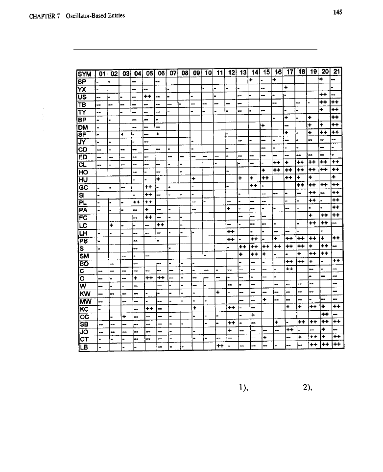
T A B L E 7 - 1
In-Sample Performance Broken Down by Test and Market
Tests I through 3: Stochastic Overbought/Oversold Models. These tests
evaluate the model with entry at the open (Test
on a limit (Test
and on a
stop (Test 3). Lane’s original Fast %K was used. The length was stepped from
5 to 25 in increments of 1. The best values for this parameter in-sample were
25, 20, and 16 (Tests 1 through 3, respectively). For the Stochastic, the tradi-
tional thresholds are 20 (lower) and 80 (upper). As a whole, these models lost
heavily in- and out-of-sample (see Table 7-3). As in previous tests, the limit
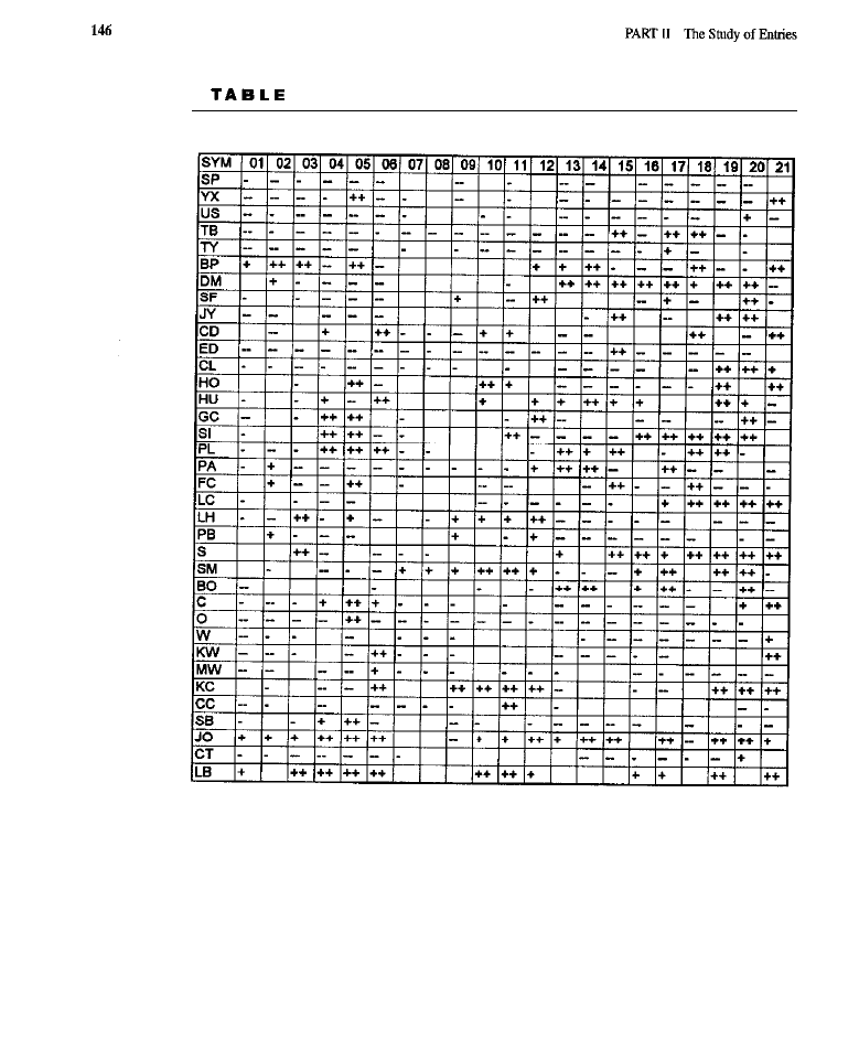
7 - 2
Out-of-Sample Performance Broken Down by Test and Market
order was the best in both samples, having the least loss per trade; the percent
of winning trades (37% in-sample, 36% out-of-sample) was also highest with
this order. The stop order was intermediate in performance, with the entry at
open being the worst. No markets traded well in either sample. Out-of-sample,
the British Pound and Orange Juice were profitable across all orders, and
Lumber, Soybeans, and Live Hogs made profits
with
a stop; other small profits
were occasionally noted, hut had no consistency. This model is among the
worst tested.
Tests 4 through 6:
Overbought/Oversold Models. The model was tested
with entry at the open (Test
on a limit (Test
and on a stop (Test 6). The
RSI was computed as suggested by its originator, Larry Williams. The length
was stepped from 5 to 2.5 in increments of 1. Across all tests, 25 was the best
value for this parameter in-sample. The traditional thresholds were used: 30
(lower) and 70 (upper). The model performed more poorly than the Stochastic
overbought/oversold one. The percentage of winning trades was extremely low,
ranging from 26% to
depending on sample and test. The average loss per
trade reached over $7,000. Net profits were better than for the Stochastic
because there were fewer trades; even though the loss per trade was greater, the
total loss was smaller. This model did not capture any market inefficiency. The
limit order was best, while the stop and open were about equal. Significantly
more markets showed positive returns, especially in Test when the limit was
used: Profits occurred in-sample for Bonds, COMEX Gold, Silver, Platinum,
Feeder Cattle, Oats, and Coffee; out-of-sample, Gold, Silver, Platinum, Feeder
Cattle, and Oats still traded profitably. Also profitable out-of-sample were the
NYFE, British Pound, Heating Oil, Corn, Sugar, Orange Juice, and Lumber.
Tests of Signal Line Models
These are essentially moving average crossover models, except that an oscillator
is substituted for prices when searching for crossovers. In this case, the moving
average is called the signal line. A short entry is signalled when the oscillator
crosses from above to below the signal line; when the oscillator does the reverse,
a long entry is generated. Since oscillators show less lag than moving averages and
less noise than raw prices, perhaps more timely and reliable signals can be gener-
ated. In Tests 7 through 12, the Stochastic and MACD are considered. The Slow
%K usually exhibits strong cyclic behavior, appropriate for use with a signal line
entry. The MACD is traditionally plotted with the signal line, even if crossovers
are not a traditional entry criteria.
Tests 7 through 9: Stochastic Signal Line Models. The model was tested with
entry at the open, on a limit, and on a stop (Tests 7 through 9, respectively).
Lane’s original Slow %K Stochastic was used because, in preliminary testing,
Fast %K produced an incredible excess of trades, resulting from very high noise
levels and the indicator pegging near its extremes. The signal line consisted of a
simple moving average of Slow
The length of the Stochastic was
stepped from 5 to 25, in increments of 1. The best values for this parameter in-
sample were 15, 14, and (Tests 7 through 9). Overall, these models lost heav-
ily on a per trade basis. Due to the large number of trades, the losses were
astronomical. The limit order was best, showing the least loss per trade and the
highest percent of winning trades across samples. Entry at the open was worst.

This model likes stops, perhaps because they act as trend filters: After
activity is detected (triggering an entry signal), before entry can occur,
the market must demonstrate reversal by moving in the direction of the trade.
Stops also performed better in countertrend moving average models, Only two
markets had positive returns in-sample, but not out-of-sample. Out-of-sample, the
stop produced a few small profits; Coffee made more than $2,000 per trade.
Tests 10 through 12: MACD Signal Line Models.
Entry at the open (Test
on
a limit (Test
and on a stop (Test 12) were examined. The classic MACD,
employing exponential moving averages, was used. The shorter moving average was
stepped from a length of 3 to a length of 15 in increments of 2; the longer moving
average was stepped from lengths of 10 through 40 in increments of 5. The moving
average serving as the signal line had a fixed traditional period of 9. This was the
best performing oscillator model thus far. In-sample, the limit order was best and
entry at open was worst. Out-of-sample, the stop was best and the limit order worst.
Out-of-sample,
stop produced the highest percentage of wins (40%) seen so far,
and the smallest loss per trade. In-sample, only Lumber was substantially profitable
with a limit. Live Hogs, Pork Bellies, Coffee, and Sugar were profitable in-sample
with a stop. Lumber, Live Hogs, Pork Bellies, and Coffee held up out-of-sample.
Many markets unprofitable in-sample, were profitable out-of-sample. The highest
number of markets traded profitably with a stop.
TESTS OF DIVERGENCE MODELS
Tests 13 through 21 examine divergences with the Stochastic oscillator, the RSI,
and the MACD. Divergence is a concept used by technical traders to describe
something easily perceived on a chart but hard to precisely define and detect algo-
rithmically. Figure 7-l shows examples of divergence. Divergence occurs when,
e.g., the market forms a lower valley, while the oscillator forms a higher valley of
a pair of valleys, indicating a buy condition; selling is the converse. Because wave
forms may be irregular, quantifying divergence is tricky. Although our detection
algorithm is elementary and imperfect, when examining charts it appears to work
well enough to objectively evaluate the usefulness of divergence.
Only buy signals will be discussed; the sells are the exact opposite. The algo-
rithm’s logic is as follows: Over a look-back (in the code,
the lowest bar in
the price series and the lowest bar produced by the oscillator are located. Several
conditions are then checked. First, the lowest bar of the price series must have
occurred at least one bar ago (there has to be a definable valley), but within the
past six bars (this valley should be close to the current bar). The lowest bar in the
price series has to occur at least four bars after the lowest bar in the look-back peri-
od for the oscillator line (the deepest valley produced by the oscillator must occur
before the deepest valley produced by the price). Another condition is that the low-
est bar produced by the oscillator line is not the
bar in the look-back period

(again, there has to be a definable bottom). Finally, the oscillator must have just
turned upward (defining the second valley as the signal about to be issued). If all
conditions are met, there is ostensibly a divergence and a buy is posted. If a buy
has not been posted, a similar set of conditions looks for peaks (instead of valleys);
the conditions are adjusted and a sell is posted if the market formed a higher high,
while the oscillator formed a lower high. This logic does a reasonable job of
detecting divergences seen on charts. Other than the entry orders, the only differ-
ence between Tests 13 through 21 is the oscillator being analyzed (in relation to
prices) for the presence of divergence.
Tests 13 through 15: Stochastic Divergence
Fast %K was used with the
standard entries. Optimization involved stepping the Stochastic length from 5 to 25
in increments of 1 and the divergence look-back from 15 to 25 by 5. The best para-
meters were length and look-back, respectively, 20 and 15 for open, 24 and 15 for
limit, 25 and 15 for stop. This model was among the worst for all orders and in both
samples. In-sample, the limit was marginally best; out-of-sample, the stop. In-Sam-
ple, across all orders, Unleaded Gasoline, Soybeans, and Soybean Meal were prof-
itable; Gold and Pork Bellies were moderately profitable with a limit. Unleaded
Gasoline held up out-of-sample across all orders. Soybeans were profitable
sample for the open and stop. More markets were profitable out-of-sample than
sample, with the stop yielding the most markets with profits. The pattern of more
profitable trading out-of-sample than in-sample is prima facie evidence that opti-
mization played no role in the outcome; instead, in recent years, some markets have
become more tradeable using such models. This may be due to fewer trends and
increased choppiness in many markets.
Tests 16 through 18:
Divergence Models.
Optimization stepped the
period
from 5 to 25 in increments of and the divergence look-back from 15 to 25 by 5.
Overall, the results were poor. h-sample, the stop was
bad, with the limit close
behind. Out-of-sample, the stop was also best, closely followed by the open. Given that
the RSI has been one of the indicators traditionally favored by traders using diver-
gence, its poor showing in these tests is noteworthy. Heating Oil was profitable for all
orders, Unleaded Gasoline
profitable for the open and stop, Light
Crude for the limit and stop. In-sample, Soybeans traded very profitably across orders;
Orange Juice, Corn, Soybean Oil, and Pork Bellies traded well with the stop.
sample, the oils were not consistently profitable, while Soybeans remained profitable
across orders; Orange Juice and Soybean Oil still traded profitably with the stop.
Tests 19
21: MACD Divergence
The length of the shorter
moving average was stepped from 3 to 15 in increments of 2; the length of the
longer moving average from 10 to 40 by 5; and the divergence look-back from 15
to 25, also by 5. Only parameter sets where the longer moving average was
ally longer than the shorter one were examined.

Finally, models that appear to work, producing positive returns in both sam-
ples!
With entry at open, trades were profitable across samples. In-sample, the
average trade made $1,393; 45% of the trades were winners; and there was only
an 8.7% (uncorrected; 99.9% corrected) probability that the results were due to
chance; both longs and shorts were profitable. Despite poor statistical significance
in-sample, there was profitability out-of-sample: The model pulled $140 per trade
(after commissions and slippage), with 38% winning trades; only shorts were
profitable.
The limit performed slightly worse in-sample, but much better out-of-sam-
ple. Figure 7-2 depicts the equity curve for entry on a limit. In-sample, the aver-
age profit per trade was $1,250 with 47% winning trades (the highest so far); longs
and shorts were profitable; and the probability was 13.1% (uncorrected; 99.9%
corrected) that the results were due to chance. Out-of-sample, the model made
$985 per trade; won 44% of the time: was profitable in long and short positions;
and was only 27.7% likely due to chance.
It-sample, the stop had the greatest dollars-per-trade return, but the smallest
number of trades; only the shorts were profitable. Out-of-sample, the system lost
$589 per trade; only short positions were profitable. Regardless of the order used,
this model had relatively few trades.
The market-by-market analysis (see Tables 7-1 and 7-2) confirms the poten-
tial of these models to make money. The largest number of markets were profitable
in-sample. Across samples, all three orders yielded profits for Light Crude and
Coffee; many other markets had profitability that held up for two of the orders, but
not for the third, e.g., Heating Oil, Live Cattle, Soybeans, Soybean Meal, and
Lumber.
SUMMARY ANALYSES
Table 7-3 provides the results broken down by the model, order, and sample. The
last two
on the right, and the last two rows on the bottom, are averages.
The numbers at the right are averaged over order type. The numbers at the bottom
have been averaged over all models.
The best results across samples were for the MACD divergence model. The
limit produced the best
results in both samples: a 12.5% return (annu-
alized) and $1,250 per trade in-sample, and a 19.5% return (annualized) and $985
per trade out-of-sample. This model is dramatically different from all others.
When considered across all order types and averaged, the overbought/over-
sold models using the RSI were worst (especially in
of dollars-per-trade).
Also among the worst were the Stochastic divergence, Stochastic
sold, and RSI divergence models.
When all models were averaged and broken down by order type, the limit
order was best and the entry at open worst.
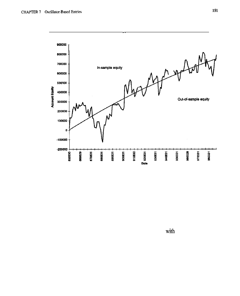
F I G U R E 7 - 2
Equity for MACD Divergence Model with Entry on a Limit
CONCLUSION
With breakouts and moving averages, a limit usually was the best overall performer,
perhaps because it minimizes transaction costs; a stop sometimes improved perfor-
mance, depending on its interaction with the entry model. For some oscillator
entries, including the profitable MACD divergence, a limit was again best. Other
oscillator models preferred the stop, perhaps due to its trend filtering quality.
There was an interaction between specific oscillators and models. The diver-
gence model, for example, worked well with the MACD, but terribly with the RSI.
Such results demonstrate that, when studying a model
an indicator compo-
nent that may be varied without altering the model’s essence, it is important to test
all model-indicator combinations as certain ones may perform dramatically better.
WHAT HAVE WE LEARNED?
n
In general, for best results, use a limit order. However, test a stop as it
sometimes works better.
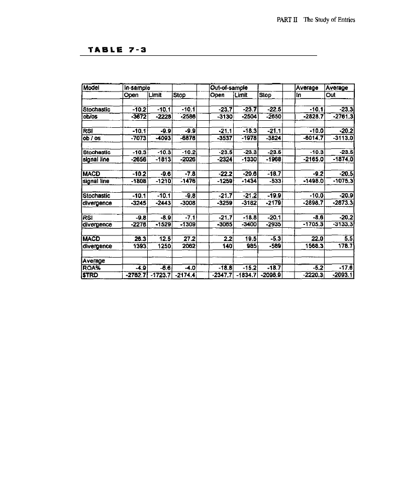
Performance of
Oscillator
Models Broken Down by Model, Order,
and Sample
. When testing a model that can be used with multiple indicators, try sever-
al to see whether any yield distinct improvements.
n
Attempt to algorithmically implement concepts normally employed in a
highly variable and subjective manner. Sometimes this can be exception-
ally difficult, requiring fuzzy logic or neural network technology, along
with other specialized methods.

C H A P T E R 8
Seasonality
that tomorrow is June 7, 1997. You need to decide whether or not to
trade. If you do trade, you will enter at the open and exit at the close. You also need
to decide how to enter the market: Should you go long or short? As part of the
decision process, you examine the behavior of the market on all June 7s that
occurred within a look-back window of some number of years (e.g., 10). You tab-
ulate the number of June 7s on which trading occurred, the average open-to-close
change in price, and the percentage of time the market rallied or collapsed.
Perhaps, in
the past
10 years, there were eight instances when the market was open
and June 7 was a trading day: of those instances. perhaps the market closed high-
er than it opened six times (75%) and the average change in price was 2.50 (a rea-
sonable figure for the S&P 500). On the basis of this information, you place a
trading order to enter long tomorrow at the open and to exit at the close. Tomorrow
evening you repeat the procedure for June 8, the evening after that for June 9, and
so on. This is one form of seasonal trading. Will you make a profit trading this
way? Will your trading at least be better than chance? These are the questions that
arise when discussing seasonal trading and that this chapter attempts to answer.
WHAT IS SEASONALITY?
The term
is used in many different ways by traders. Some construe
seasonality as events that are strictly related the four seasons, e.g., the increased
demand for heating oil in the winter or gasoline in the summer. Others have a more
liberal interpretation that includes weather patterns and election cycles.
Over the years, a number of articles in academic journals have demonstrated
that stocks show larger returns around the first of each month. There has been some

discussion of the so-called January Effect, in which stocks tend to rise in January.
(1991) used seasonal cycles in his own trading, providing as an example
a chart for EXABYTE stock with strong seasonal patterns marked. He also dis-
cussed another phenomenon, sometimes observed with seasonal patterns, in which
the highs and lows occasionally invert, a pattern that we also have witnessed and
that may be worth exploring. Other factors that influence various markets have def-
inite dates of occurrence and so should induce seasonal effects; e.g., the dates for
filing taxes occur at the same time every year. The legendary trader, Gann, appar-
ently made heavy use of recurrent yearly behavior in his trading. Bernstein’s (1995)
home-study course on seasonality suggests trading off significant tops and bottoms,
and when there has been consistent movement in a tradable over a number of years;
this approach, as well as
may tend to involve trades lasting several
weeks to several months.
In 1990, we first published the Calendar Effects Chart, a set of tables and a
chart that show date-specific behavior in the S&P 500 cash index. The chart illus-
trates a general up-trend from January through September, and then an up and
down decline until October 24. The market then, on average, bottoms, after which
time it steeply rises until the end of the year. On a more detailed level, rapid gains
seem to occur throughout most of January, the
half of April, and the first half
of June. A peak can be seen on October 8, and a very steep decline that leads to a
bottom on October 24. When the tables and chart for this publication were gener-
ated, extreme movements were clipped at
percent to prevent them from having
undue influence on the results. Consequently, the steep decline in October, and the
other patterns mentioned, cannot be attributed to events in specific years, for
instance, the crash in 1987. For some dates, there were incredibly consistent pat-
terns; e.g., if an entry occurred on the close of April 14 and the trade was exited
one day later, over 90% of the time a small profit would have been made. Entry on
May 6, with exit one day later, resulted in a profit 100% of the time, as did entry
on July 13. The market declined 90% of the time from October 18 to 19, and 89%
of the time from October 16 to 17. Although the crash may have involved a much
greater than normal amount of movement, the presence of a decline at the time
when the crash occurred was not at all unexpected. In an attempt to capture
probability, short-term movements, the Calendar Effects Chart could have been
used to enter trades that last one or two days. For example, such a methodology
would have caused a trader to go short at the close on October 16 and exit on
October 19, thus capturing the crash. The data contained in this publication could
also have been used to help maintain positions during periods of steep ascent or
decline.
There have been other studies indicating the presence of strong seasonal effects
in the market that can be exploited for profitable trading. An investigation we con-
ducted (Katz and McCormick, April 1997) found that short-term seasonal behavior
could be used to trade the S&P
The system used
fast moving average

crossovers that were computed on seasonally anticipated prices. Because the antici-
pated prices could be computed at least one year ahead, lag in the moving average
crossover was easily compensated for with a displacement that enabled the system
to take trades at crossovers occurring several days after the fact. The trades taken by
the system typically lasted between 7 and 8 days, a fairly short-term seasonal trad-
ing model. The system was profitable: It pulled an astonishing $329,900 from the
S&P 500 between January 3.1986, and November 8, 1996. The test did not include
transaction costs, but even with $15 round-turn commissions and $75 per trade slip-
page, a profit of $298,310 (about a 10% reduction) resulted. The return on account
was
not annualized; assuming fixed contract trading, this amounted to over
70% per year, annualized, on a constant one-contract, no-reinvestment basis. There
were 351 trades taken, of which 60% were winners. Both the longs and
were
profitable. The average trade pulled $939 from the market-not bad for a simple,
trading model, Findings like these suggest there are strong sea-
sonal patterns in the markets producing inefficiencies that can be exploited by
traders, and that are worthy of investigation.
For our current purposes,
is defined as cyclic or recurrent phe-
nomena that are consistently linked to the calendar. The term is being used in a
broad sense to mean market behavior related to the time of the year or to particular
dates, including anniversaries of critical events (e.g., the October 16, 1987, crash).
In short, seasonality is being construed as calendar-related cyclic phenomena. It
should be made clear, however, that while all seasonality is cyclic, not all cycles are
seasonal.
GENERATING SEASONAL ENTRIES
There are many ways to time entries using seasonal rhythms. Two basic approaches
will be examined: momentum and crossover. To calculate momentum, a series of
price changes is computed and
centered smoothing
(a smoothing
induces no
delays or phase shifts, in
case, a centered triangular moving average) is applied.
Each price change (or difference) in the series of price changes is then normalized:
It is divided by the
average true range. For every bar, the date is determined.
Instances of the same date are then found in the past (or perhaps future). For each
such instance, the momentum is examined. The average of the momentums becomes
the value placed in the seasonal momentum series for the current
The seasonal
series measures the expected rate of change (or momentum) in prices at
a given time. It is based on the historical movement of prices on the specified date
in different years. The number in the seasonal momentum series for the current bar
is determined only by events about 1 year or more ago. This is why it is possible to
use the centered moving average and other techniques that look ahead in time, rela-
tive to the bar
considered. Entries are taken as follows: When the seasonal
momentum crosses above some positive threshold, a buy is posted. When the

156
momentum crosses below some negative threshold, a sell is posted. Buying or sell-
ing can happen on any of the standard three orders: at open, on limit, or on stop.
Entries may also be generated by computing the price differences, normalizing
them, applying an integration or summing procedure to the series (to obtain a kind
of pseudo-price series, based on previous instances of each date), and then applying
a moving average crossover model to the series. Because the value at any bar in the
series is determined only by bars that are about 1 year old or older, the delay in the
crossovers can be compensated for by simply looking ahead a small number of bars.
Both of the methods described above arc somewhat
in nature; i.e.,
they do not require specific information about which dates a buy or sell order
should be placed. The adaptive quality of the aforementioned methods is impor-
tant since different markets respond to seasonal influences in different ways, a fact
that logic, as well as our earlier research, supports.
In the current study, several rules for handling confirmations and inversions
are also tested to determine whether better results can be obtained over the basic
models.
means additional data is available that supports the signals
produced by the model. For example, suppose a model generated a buy signal
for a given bar. If everything is behaving as it should, the market should be form-
ing a bottom around the time of the buy. If, however, the market is forming a top,
the buy signal might be suspect, in that the market may not be adhering to its typ-
ical seasonal timing. When such apparently contradictory circumstances exist, it
would be helpful to have additional criteria to use in deciding whether to act upon
the signal, in determining if it is correct. The
model
implements the crossover model with an additional rule that must be satisfied
before the signal to buy or sell can be acted upon: If a buy signal is issued, the
Slow %K on the signal bar must be less than
meaning the market is at or near
the bottom of its recent range. If a sell signal is issued, Slow %K must be greater
than
indicating that the market is at or near the top of its range, as would be
expected if following its characteristic seasonal behavior.
inversion
model
adds yet another element: If a buy signal is issued by the basic
model, and the market is near the top of its range (Slow %K greater than
then it is assumed that an inversion has occurred and, instead of issuing a buy sig-
nal, a sell signal is posted. If a sell signal is generated, but the market is near the
bottom of its range (Slow %K less than
a buy signal is issued.
CHARACTERISTICS OF SEASONAL ENTRIES
Consider trading a simple moving average crossover system. Such a system is
usually good at capturing trends, but it lags the market and experiences frequent
whipsaws. If slower moving averages are used, the whipsaws can be avoided,
but the lag is made worse. Now add seasonality to the equation, The trend-fol-
lowing moving average system is applied, not to a series of prices, but to a

series that captures the seasonal ebb and flow of the market. Then compute the
seasonal series so it represents that ebb and flow, as it will be several days from
now-just far enough ahead to cancel out the annoying lag! The result: A sys-
tem without lag (despite the use of slow, smooth, moving averages) that follows
seasonal trends. The ability to remove lag in this way stems from one of the
characteristics of seasonality: Seasonal patterns can be estimated far in
advance. In other words, seasonality-based models are
predictive,
as opposed
to merely responsive.
Since seasonality-based models are predictive, and allow turning points to be
identified before their occurrence, seasonal-based trading lends itself to
tertrend trading styles. Moreover, because predictions can be made far in advance,
very high quality smoothing can be applied. Therefore, the kind of whipsaw trad-
ing encountered in responsive models is reduced or eliminated. Another nice char-
acteristic of seasonality is the ability to know days, weeks, months, or even years
in advance when trades will occur--certainly a convenience.
Seasonality also has a downside. The degree to which any given market may
be predicted using a seasonal model may be poor. Although there may be few
whipsaws, the typical trade may not be very profitable or likely to win. If inver-
sions do occur, but the trading model being used was not designed to take them
into account, sharp losses could be experienced because the trader could end up
going short at an exact bottom, or long at an exact top.
The extent to which seasonal models are predictive and useful and the pos-
sibility that inversion phenomena do exist and need to be considered are questions
for empirical study.
ORDERS USED TO EFFECT SEASONAL ENTRIES
Entries based on seasonality may be effected in at least three ways: with stops,
limits, or market orders. While a particular entry option may work especially well
with a particular model, any entry may be used with any model.
Entry orders themselves have their own advantages and disadvantages. The
advantage of a market or&r is that no signaled entry will be missed.
Stop orders
ensure that no significant trends (in a trend-following model) will elude the trader,
and that entry will not occur without confirmation by movement in favor of the
trade (possibly beneficial in some countertrend models). The disadvantages are
greater slippage and less favorable entry prices, A
limit order
gets the trader the
best price and minimizes transaction costs. However, important trends may be
missed while waiting indefinitely for a
to the limit price. In
tertrend models, a limit order may occasionally worsen the entry price. The entry
order may be tilled at the limit price, rather than at a price determined by the neg-
ative slippage that sometimes occurs when the market is moving against the trade
at the time of entry!

158
TEST METHODOLOGY
The data sample used throughout the tests of seasonal entry methods extends from
August 1, 1985, to December 31, 1994 (the in-sample period), and from January
1995, through February 1999 (the out-of-sample period). For seasonality
studies, an in-sample period of only 10 years means there is a shortage of data on
which to develop the model. When generating seasonal entries was discussed,
mention was made about calculating seasonal momentum (or average price behav-
ior) based on equivalent dates in previous years. Because of the data shortage,
when considering the in-sample data, calculations will be based not only on past
years, but also on future years.
is accomplished using
“jackknife.”
Target dates are run throughout the series, bar after bar. If only past years are
included, for the early data points, there are very few past years or none at all.
Since it takes at least 6 years of past
data
to get a reasonable seasonal average,
there would be no seasonality calculations for most of the in-sample period, which
itself is only 10 years. Consequently, there is very little data on which to optimize
essential parameters or determine how seasonal models perform on the in-sample
data.
The jackknife,
a well-known statistical technique (also known as the
one-out method”), helps solve the data shortage problem
Suppose a seasonality estimate for June 1, 1987, is being calculated. If
only past data from the in-sample period is used, the estimate would be based on
data from 1986 and 1985. If, however, the jackknife is applied, not only would
data from the past be available, but so would data from the “future,” i.e., the
other years of the in-sample period (1988 through 1994). If the year (1987) that
serves as the target bar for the calculations is removed from the in-sample period,
the seasonality estimate for that bar would now be based on 9 years of data, a
reasonably adequate sample. The jackknife procedure is justified because the
data being examined to make the prediction is fairly independent of the data
actually being predicted by the seasonality estimate. Since the data used in gen-
erating the prediction is at least 1 year away from the target date, it is not con-
taminated with current market behavior. The process’provides an effectively
larger sample than could otherwise be obtained, and does so without seriously
compromising the available number of degrees of freedom.
For bars in the out-of-sample period, all past years are
used
to generate the sea-
sonal&y estimates. For example, to calculate the seasonality for January 14, 1999,
the &past-years technique
is used: Data from 1998 all the way back to 1985 are
included in the analysis. In this way, no calculation for the out-of-sample period is
ever based on any future or current data.
All the tests that follow are performed using seasonal entries to trade a diversi-
fied portfolio of commodities. The exits are the standard ones, used throughout
book to study entry models. Trades are closed out either when an
in the oppos-
ing direction occurs or when the standard exit closes the trade, whichever comes first.
The test platform is also standard. Here is the code for the seasonal trading tests:
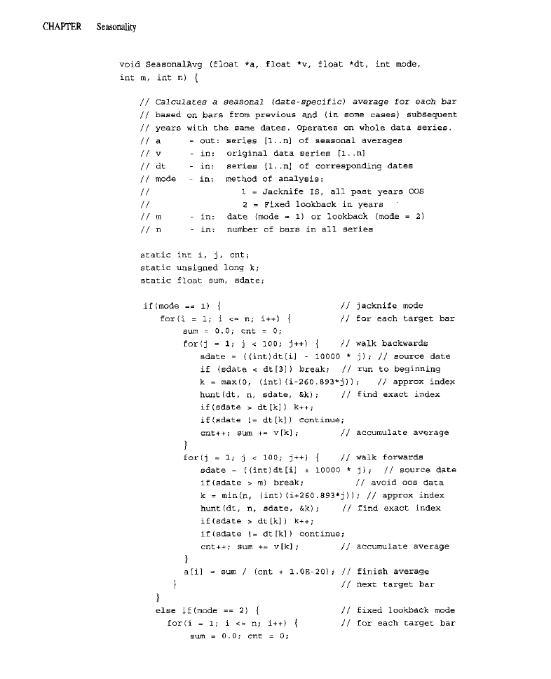
8
159

160


162
3
==
stochastic
break;
default:
invalid
step through bare
to simulate actual trading
1; cb
(
take no trades before the in-sample period
same
setting
(
0.0; continue; )
execute any pending orders and
closing equity
3
I=
buffer overflow");
avoid placing
on possibly limit-locked days
continue;
generate entry
stop prices and limit prices
for all
entry models
signal
(
1:
basic
momentum entry model
cb disp;
thresh
signal = 1;
else
signal -1;
basic crossover
model
cb disp;

process next

After declaring local variables and arrays, the first major block of code
copies various parameters to local variables for more convenient and understand-
able reference. The parameters are described in comments in this block of code.
The next block of code performs all computations that are carried out on
complete time series. The
average true range is calculated and saved in a
vector
it will be used later for the placement of money management stops
and profit targets in
standard exit strategy. The average true range in this vec-
tor (or data series) is also used to normalize the price changes in the code that
immediately follows.
After calculating the average true range, normalized and clipped price
changes are calculated. Each bar in the
reflects the change in price from
the close of the previous bar to the close of the current bar. The price changes are
normalized by dividing them by the average true range. They are then clipped to
limit the influence of sharp spikes or statistical oudiers. Normalization is performed
because markets change in their volatility over time, sometimes very dramatically.
For example, the current S&P 500 has a price almost five or more times its price 15
years ago, with a corresponding increase in the size of the average daily move. If
the price changes were not normalized and represented in terms of recent volatili-
ty, any seasonal estimate conducted over a number of years would be biased. The
years with greater volatility would contribute more to
estimate than the years
with lesser volatility. In the case of the S&P 500, the most recent years would
almost totally dominate the picture. Using normalized price changes, each year
contributes about equally. Clipping to remove
is performed so the occa-
sional, abnormal price change does not skew the estimates. Clipping is performed
at -2 and
average true range units.
The
selection then determines which calculations occur next. A
modeltype
of 1 selects the basic momentum model. The seasonals are computed
from the clipped and normalized price changes, the jackknife is used on the
sample period, and the all-past-years technique is used for the out-of-sample period.
These calculations are accomplished with a call to the function called
The series of seasonal estimates is then smoothed using a moving
average of the type, specified by the parameter
and of a length set by
another parameter. A series of average absolute deviations of the seasonal
momentums is then computed. This series is nothing more than a
simple
moving average of the absolute values of seasonal momentum, which is used in
later computations of threshold values. The
of
and 4 all represent
variations of the crossover model. The seasonals are computed, and then the sea-
sonal estimates of price change for every bar are integrated (a running sum is cal-
culated), creating a new series that behaves almost like a price series. The
synthesized, price-like series represents the movement in prices based on typical
behavior in previous and perhaps future years. Two moving averages are then
computed:
(a moving average of the integrated seasonal time series of

CHAPTER
165
having a length of
and ma2 (used as a signal line for detecting
crossovers, calculated by taking a moving average of
the kind of average
taken is again specified by
and the length by
If the
is
3 or 4, additional calculations are performed for models in which confirmation
and/or inversions are detected; in the current study, a
Fast %K is calculated
and saved in the vector
The next block of code consists of a loop that steps sequentially through all
bars in the data series. This loop is the
one that has been seen in every pre-
vious chapter on entry strategies. The first few lines of code deal with such issues
as updating the simulator, calculating the number of contracts to trade, and avoid-
ing limit-locked days. The next few lines generate entry signals for all the
ality-based entry models. Depending on the value of the modeltype parameter,
either of four different approaches is used to generate entry signals.
A
of 1 represents the basic momentum threshold entry model. A
threshold is calculated by multiplying a threshold-determining parameter (thresh)
by the average absolute deviation of the seasonal momentum over the past 100 bars,
A long signal is issued if the seasonal momentum
on the current bar plus a
displacement parameter
crosses above the threshold. If the seasonal
turn, at the current bar plus the displacement, crosses below the negative of the
threshold, a sell signal is generated. In other words, if sufficiently strong seasonal
momentum is predicted for a given date, plus or minus
number of days or bars
then a trade is taken in the direction of the expected movement.
For
2, which represents the basic crossover entry model, the
ing averages of the integrated
at the current bar plus a displacement fac-
tor, are calculated. If the first moving average crosses above the second, a buy
is
generated. If it crosses below, a sell is generated. The displacement factor allows
the model to look for such crossings some number of days down the line (ahead
in time). In this manner, the displacement can neutralize the lag involved in the
moving averages. Because the seasonal averages are based on data that is usually
a year old, it is perfectly acceptable to look ahead several days.
A
of 3 represents the same crossover model, but with the addition
of confirmation. Confirmation is achieved by checking the Stochastic oscillator of
the actual price series to determine whether it is consistent with what one would
be expected if the market were acting in a seasonal fashion.
If
is 4, the crossover model, with the addition of confirmation and
inversion, is selected. When there is a
of 4, a buy signal is issued if the
first moving average crosses above the second, and the seasonal pattern is con-
firmed by a Stochastic of less than 25. The model assumes that an inversion has
occurred and issues a sell signal if the Stochastic is over 75. If the
moving
average crosses below the second moving average, and the normal seasonal pat-
tern is confirmed by a Stochastic that is over 75, a sell signal is issued. Inversion
is assumed and a buy signal issued if the Stochastic is less than 25.
Finally, the limit price
is set at the midpoint of the current
The
stop price
for entry on a stop, is set at the close of the current bar plus
(if entering long) or minus (if entering short) one-half of the
average true
range. The remaining code blocks are identical to those in previous chapters: They
involve actually posting trades using the specified order
and instruct-
ing the simulator to employ the standard exit strategy.
T E S T R E S U L T S
Tests are performed on two seasonality-based entry models: the crossover model
(both with and without confirmation and inversions) and the momentum model.
Each model is examined using the usual three entry orders: enter at open, on limit,
and on stop.
Tables 8-l and 8-2 provide information on the specific commodities that the
model traded profitably, and those that lost, for the in-sample (Table
and
of-sample (Table 8-2) runs. The
column represents the market being studied.
The rightmost column
contains the number of profitable tests for a given
market. The numbers in the first row represent test identifiers. The last row
contains the number of markets on which a given model was profitable.
The data in these tables provide relatively detailed information about which markets
are and are not profitable when traded by each of the models: One dash indicates
a moderate loss per trade, i.e., $2,000 to
two dashes
represent a large loss
per trade, i.e.,
or more; one plus sign (+) means a moderate profit per trade,
i.e., $1,000 to
two pluses (+ +) indicate a large gain per trade, i.e., $2,000
or more; and a blank cell means that the loss was between $0 and $1,999 or the prof-
it was between $0 and $1,000 per trade. (For information about the various markets
and their symbols, see Table II-1 in the “Introduction” to Part II.)
Tests of the Basic Crossover Model
A simple moving average
of a specified length
was computed for the
integrated, price-like seasonality series. A second moving average
was taken of
the
moving average. A buy signal was generated when
crossed above
A sell signal was generated when
crossed below
(This is the same
average crossover model discussed in the chapter on moving averages, except here it
is computed on a predicted, seasonal series, rather than on prices.) The entries were
effected by either a market at open (Test a limit (Test
or a stop order (Test 3).
Optimization for these tests involved stepping the length of the moving aver-
ages
from 5 to 20 in increments of 5 and the displacement
from 0
to 20 in increments of 1. For entry at the open, the best performance (in terms of
in-sample risk-to-reward ratio) was achieved with a moving average length of 20
and a displacement of 5. Entry on a limit was best with a length of 20 and a

T A B L E B - l
In-Sample Performance Broken Down by Test and Market
placement of 8. Entry on a stop required a length of 20 and a displacement of 6.
The model seemed to prefer longer moving averages (more smoothing), and some-
what earlier signals were required by the limit order when compared with the stop
or market-at-open orders.
In-sample, none of the results were profitable when both long and short posi-
tions were traded. However, the losses were much smaller on a per-trade basis than
those observed in many of the other tests presented in earlier chapters. The stop
order performed best. The market-at-open order performed worst. The limit order
came in not too
behind the stop. For both the stop and limit orders, trading was
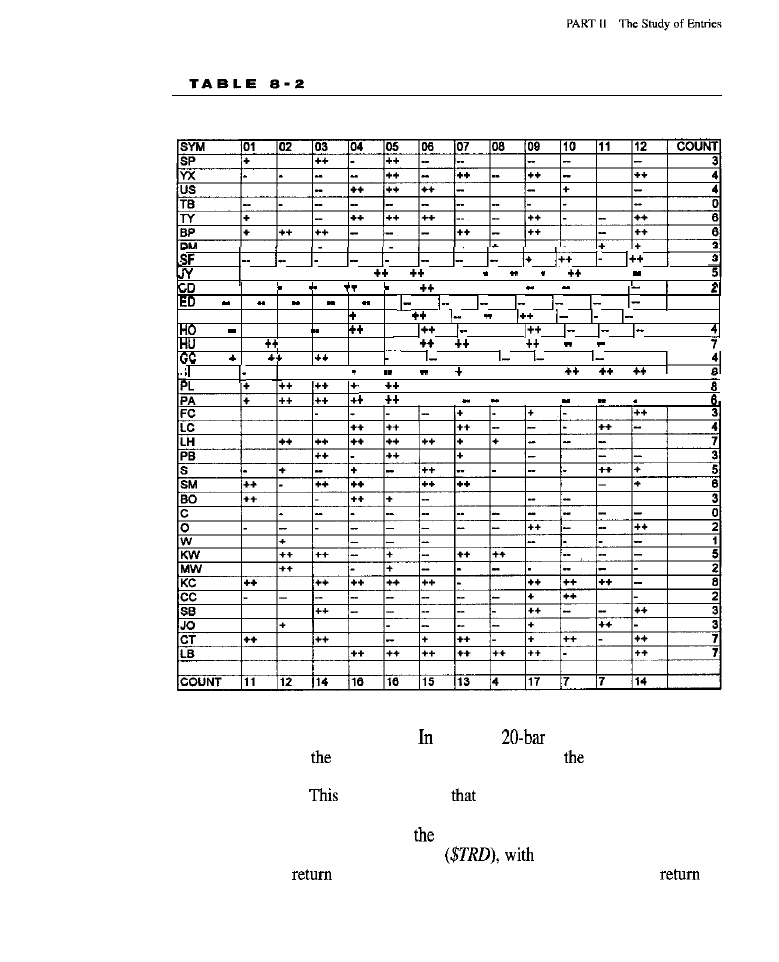
Out-of-Sample Performance Broken Down by Test and Market
.
I-
. .
++
+
I
0
CL
+
,
.
++
++
++ ++
I+
I-
s
+
++
,
++
I-
++
I-
++
++
I
actually profitable for long positions.
all cases,
moving averages provided
the best results, but
displacement varied depending on
order. A look-ahead
of 5 bars was optimal for entry at tbe open, 8 bars for entry on a limit, and 6 bars
for entry on a stop.
makes sense, in
one would want to post a limit order
earlier than a market-on-open order so as to give the limit some time to be filled.
Out-of-sample, the results showed
same ordering of overall performance as
measured by the average profit per trade
the stop order actually pro-
ducing a positive
of $576 per trade, representing an 8.3% annual
on
account; this system, although not great, was actually profitable on recent data. For

stop entry, both in- and out-of-sample trading was profitable when only the long
trades were considered, but the short side lost in both samples. This is a pattern that
has been observed a number of times in the various tests. The percentage of wins
for all orders and samples was between 40 and 43%.
It is interesting that, even for the losing variations, the losses here were much
smaller than what seems typical for many of the models so far tested.
With entry at the open, equity declined until November 1988. It retraced
approximately 50% of the way until July 1989, making a small U-shaped forma-
tion, with
second of a double-top around November 1990. Equity then declined
rather steeply until November 1992 and, in a more choppy fashion, throughout tbe
remainder of the in-sample period and the
third of the out-of-sample period.
The decline ended in April 1996 when equity gradually climbed throughout the
remainder of the out-of-sample period.
With entry on a limit, equity was fairly flat until January 1987, rose very
rapidly to a peak in May 1987, and then declined until November 1992. From then
through July 1994, equity rose steeply. Afterward, choppy performance was
observed with no significant trend.
The stop order produced strong equity growth until June 1988. Equity then
declined in a choppy fashion through most of the in-sample period and about the
first quarter of the out-of-sample period. It reached bottom in December 1995 and
then rose sharply through the end of the out-of-sample period in February 1999.
Across all three entry orders, the best-performing market was Unleaded
Gasoline, in which strong, consistent profits were observed in both samples.
Palladium was also a strong market for this model:
the entry at open and entry
on limit produced profits in- and out-of-sample, with the entry on limit having
strong profits in both samples, and the entry on stop producing strong profits
of-sample and neutral results in-sample. Live Hogs was another good market to
trade seasonally: Every order type yielded profits in-sample, while two of the three
order types yielded profits out-of-sample; both the limit and stop orders were prof-
itable in both samples. Yet another good market to trade with this model is Coffee:
All
orders produced in-sample profits, while the market at open and stop
orders produced strong profits out-of-sample. Finally, Cotton did not do too badly:
The stop order yielded strong profits in both samples, and no order resulted in
strong losses in either sample. Finding good performance for Unleaded Gasoline is
totally in accord with expectations. What is moderately surprising is that Heating
Oil, for which there is a strong seasonal demand characteristic, was only profitable
in both samples when using the limit order. Coffee also traditionally has strong sea-
sonal patterns caused by, e.g., recurrent frosts that damage crops, create shortages,
and drive up prices. Surprisingly, the wheats did not produce many profits in-sample.
The only exception was a small profit for Minnesota Wheat with a limit order. More
profits in the wheat group were seen out-of-sample, where the limit order led to
profitable trading in all three wheat markets and the stop order in Kansas Wheat.

A number of other markets showed profitable, but less consistent, trading across
sample and order type. Again, it is impressive to see the great number of markets
that trade well across both samples, especially when compared with many of the
other models that have been tested in the preceding chapters.
It is also interesting that there is a discrepancy between the performance of the
seasonality model in the current tests and in our earlier tests of the S&P 500 (Katz
and McCormick, April 1997). The differences are probably due to such factors as
tuning. In the earlier tests, the moving averages were specifically toned to the S&P
500; in the current tests, they were tuned to the entire portfolio. Moreover, com-
pared with other markets, the seasonal behavior of the S&P 500 appears to involve
fairly rapid movements and, therefore, requires a much shorter moving average to
achieve optimal results. Finally, the earlier tests did not use separate exits and so a
seasonal trend lasting several weeks could be captured. In the current test, only the
first
days could be captured, after which time the standard exit closes out the
trade. It is likely that the performance observed, not just on the S&P 500, but on all
the markets in the portfolio, would be better if the standard exit were replaced with
an exit capable of holding onto a sustained
Tests of the Basic Momentum Model
For the momentum model, the unintegrated seasonal price change series was
smoothed with a centered simple moving average of a specified length
The centered average introduces no lag because it examines as many future data
points, relative to the current bar, as it does past data points. The use of a centered
moving average is legitimate, because the seasonality estimate at the current bar is
based on data that is at least 1 year away. For this series of smoothed seasonal
price changes, a series of average absolute deviations was computed: To produce
the desired result, the absolute value for each bar in the smoothed seasonal series
was computed and a
simple moving average was taken. A buy signal was
issued if the seasonal momentum, at the current bar plus some displacement
was greater than some multiple (thresh) of the average absolute deviation
of the seasonal momentum. A sell signal was issued if the seasonal momentum, at
the same displaced bar, was less than minus the same multiple of the average
absolute deviation. Entries were executed at the open (Test
on a limit (Test
or on a stop (Test 6).
Optimization was carried out for the length of the moving averages, the dis-
placement, and the threshold. The length was stepped from 5 to 15 in increments
of 5; the displacement from 1 to 10 in steps of 1; and the threshold from 1.5 to 2.5
in increments of 0.5. The best in-sample performance was observed with a length
of 15 and a threshold of 2.5, regardless of entry order. For the market at open and
for the stop a displacement of 2 was required. The limit worked best with a dis-
placement of 1.
agreement with expectations, these displacements are much

smaller than those that were optimal for the crossover model where there was a
need to compensate for
lag associated
the moving averages.
Overall, the results were much poorer than for the seasonal crossover
model. In-sample, profitability was only observed with the stop order. No prof-
itability was observed out-of-sample, regardless of the order. The losses on a
trade basis were quite heavy. Interestingly, the long side
less well
overall than the short side. This reverses the usual pattern of better-performing
long trades than short ones.
With both entry at open and on limit, equity declined in a choppy fashion
from the beginning of
in-sample period through the end of the out-of-sample
period. The decline was less steep with the limit order than with entry at open.
With the stop order, equity was choppy, but basically flat, until
1990, when
it began a very steep ascent, reaching a peak in September 1990. Equity then
showed steady erosion through the remaining half of the in-sample and most of
the out-of-sample periods. The curve flattened out, but remained choppy, after
April 1997.
The model traded the T-Bonds, IO-Year Notes, Japanese Yen, Light Crude,
Heating Oil, Unleaded Gasoline, Live Hogs, and Coffee fairly well both in- and
of-sample. For example, T-Bonds and
Notes were very profitable in both
samples when using either the limit or stop orders.
performed best with
the stop, showing heavy profits in both samples, but was profitable with the other
orders as well. The same was true for Light Crude. Heating Oil showed heavy prof-
its with the entry at open and on stop in both samples, but not with entry on limit,
This was also true for Unleaded Gasoline. Live Hogs performed best, showing heavy
profits in both samples, with entry at open or on stop. This market was profitable
with all three orders in both samples. Coffee was also profitable with all
orders
on both samples, with the strongest and most consistent profits being with the stop.
For the most part, this model showed losses on the wheats.
In-sample, 15 markets were profitable to one degree or another using a stop,
13 using a market order at the open, and 9 using a limit. Out-of-sample, the num-
bers were 15, 16, and 16, respectively, for the stop, open, and limit.
Even though the momentum model performed more poorly on the entire
portfolio, it performed better on a larger number of individual markets than did the
crossover model. The momentum model, if traded on markets
appropriate
seasonal behavior, can produce good results.
Tests of the Crossover Model with Confirmation
This model is identical to the basic crossover model discussed earlier, except that
entries were only taken if seasonal market behavior was
by an appropri-
ate reading of the Fast %K Stochastic. Specifically, if the seasonal crossover sug-
gested a buy, the buy was only acted upon if the Fast %K was below 25%; i.e., the

market has to be declining or near a bottom (as would be expected on the basis of
the seasonal buy) before a buy can occur, Likewise, a seasonal sell was not taken
unless the market was near a top, as shown by a Fast %K greater than 75%. As
always, the standard exits were used. Entries were executed at the
(Test
on
a limit (Test
or on a stop (Test 9).
Optimization for these tests involved stepping the length of the moving averages
from to 20 in increments of 5
and the displacement
from 0 to
20 in increments of 1
For entry at the open, a moving average length of and
a displacement of 7 were best. Entry on a limit was best with a length of 15 and a dis-
placement of 6. Entry on a stop required a length of 20 and a displacement of 9.
On a per-trade basis, the use of confirmation by the Fast %K worsened the
results for both sampling periods when entry was at the open or on a limit; with
both of these orders, trades lost heavily in both samples. When the confirmed sea-
sonal was implemented using a stop order for entry, relatively profitable perfor-
mance in both samples was seen. In-sample, the average trade pulled $846 from
the market, while the average trade pulled $1,677 out of the market in the verifi-
cation sample. In-sample, 41% of the trades were profitable and the annual return
was 5.8%. The statistical significance is not great, but at least it is better than
chance; both long and short positions were profitable. Out-of-sample, 44% of the
trades were winners, the return on account was
and there was a better than
77% chance that the model was detecting a real market inefficiency; both longs
and shorts were profitable. Compared with other systems, the number of trades
taken was somewhat low. There were only 292 trades in-sample and 121
sample. All in all, we again have a profitable model. Seasonality seems to have
validity as a principle for entering trades.
The equity curve for entry at open showed a gradual decline until May 1989.
It was then fairly flat until August 1993, when equity began to decline through the
remainder of the in-sample period and most of the out-of-sample period. The limit
order was somewhat similar, but the declines in equity were less steep. For the stop
order, the picture was vastly different. Equity declined at a rapid pace until May
1987. Then it began to rise at an accelerating rate, reaching a peak in June 1995,
the early part of the out-of-sample period. Thereafter, equity was close to flat. The
greatest gains in equity for the stop order occurred between June 1990 and May
1991,
1993 and September 1993, and between January 1995 and June
1995. The last surge in equity was during the out-of-sample period.
Compared with the previous two models, there were fewer markets with con-
sistent profitability across all or most of the order types. Lumber was the only mar-
ket that showed profitability across all three order types both in- and
out-of-sample. Unleaded Gasoline yielded profits across all three order types in-
sample, and was highly profitable out-of-sample with entry at open or on stop.
Coffee and Cocoa were profitable for all order types in-sample, but profitable only
for the stop order out-of-sample. For the stop order, the NYFE, Silver, Palladium,
8
173
Light Crude, Lumber, and Coffee were highly profitable in both samples. Again,
there was no profitability for the wheats. There was enough consistency for this
model to be tradable using a stop order and focusing on appropriate markets.
Tests of the Crossover Model with Confirmatlon and
Inversions
This model is the same as the crossover model with confirmation. However, addi-
tional trades were taken where inversions may have occurred; i.e., if a seasonal
buy was signaled by a crossover, but the market was going up or near a top (as
indicated by the Fast %K being greater than
a sell signal was posted. The
assumption with this model is that the usual seasonal cycle may have inverted or
flipped over, where a top is formed instead of a bottom. Likewise, if the crossover
signaled a sell, but the Fast %K indicated that the market was down by being less
than
a buy was posted. These signals
issued in addition to those
described in the crossover with confirmation model. Entries were executed at the
open (Test IO), on a limit (Test
or on a stop (Test 12).
Optimization for these tests involved stepping the length of the moving
averages
from 5 to 20 in increments of (PI) and the displacement
from 0 to 20 in increments of 1
For entry at the open, a
average length of 15 and a displacement of 2 were best. Entry on a limit was
best with a length of 20 and a displacement of 4. Entry on a stop again required
a length of 20 and a displacement of 9.
For entry at the open, the equity curve showed a smooth, severe decline from
one end of the sampling period to the other. There was a steeply declining equity
curve for the limit order, although the overall decline was roughly half that of the
one for entry at open. For entry on stop, the curve declined until May 1987. It then
became
choppy but essentially flat until August 1993. From August 1993
until June 1995, the curve steeply accelerated, but turned around and sharply
declined throughout the rest of the out-of-sample period. Adding the inversion ele-
ment was destructive to the crossover model. The seasonal patterns studied appar-
ently do not evidence frequent inversions, at least not insofar as is detectable by
the approach used.
Adding the inversion signals to the model dramatically worsened perfor-
mance on a per-trade basis across all entry orders, Losses were seen for every
combination of sample and order type, except for a very small profit with a stop
in the out-of-sample period. There were no markets that showed consistently good
trading across multiple order types in both samples, although there were isolated
instances of strong profits for a particular order type in certain markets. The
again traded very profitably with a stop order, as did IO-Year Notes, in both sam-
ples. Platinum and Silver also traded well in- and out-of-sample with a stop order.
Soybeans traded
profitably with a stop order in-sample, but only somewhat
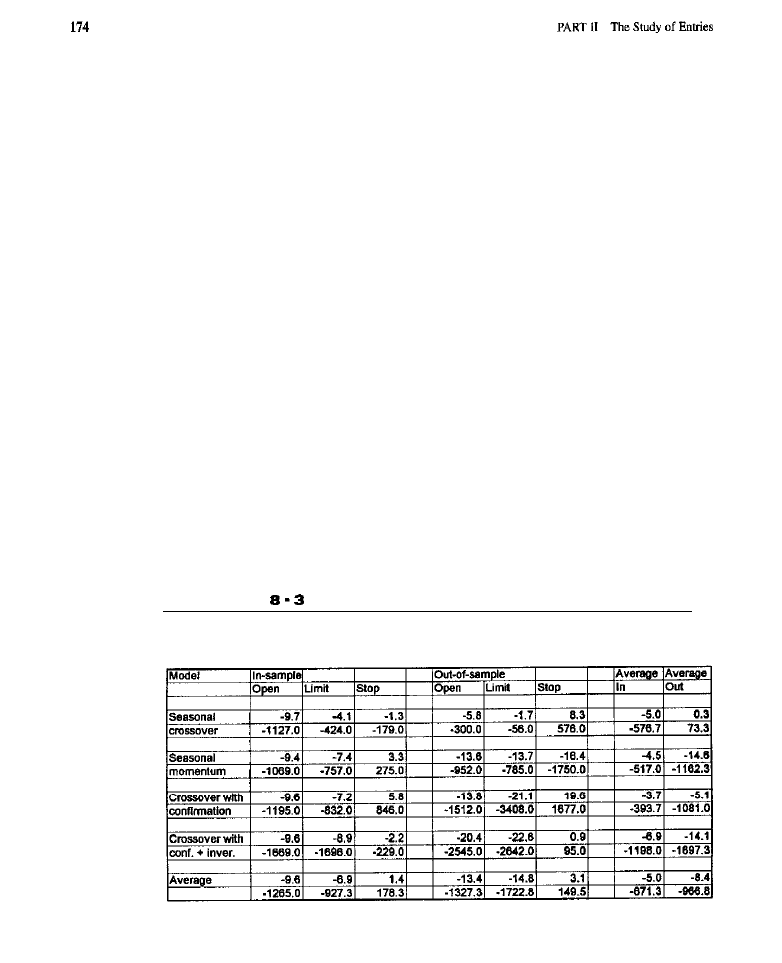
profitably out-of-sample. There were consistent losses, or no profits at all, across
all orders and samples for the wheats.
Summary Analyses
Results from the different tests were combined into one table and two charts for
overall analysis. Table 8-3 provides performance numbers broken down by sample,
entry order, and model. For each model, there are two rows of numbers: The first
row contains the figures for annualized return-on-account, and the second row con-
tains the average dollar profit or loss per trade. The two rightmost columns contain
averages across all order types for the in-sample and out-of-sample performance.
The last two rows contain the average across all models for each type of order.
Of the three types of orders, it is evident that the stop performed best. The
limit and entry at open performed about equally well, but much worse than the stop.
In fact, for the stop, the average across all four models actually showed a positive
return and small profits on a per-trade basis both in-sample and out-of-sample.
When examining models averaged across all order types, the in-sample per-
formance was best using the crossover-with-confirmation model and worst for
the crossover-with-confirmation and inversion model. Out-of-sample, the basic
crossover model showed the best performance, while the crossover with confir-
mation and inversion had the worst.
As can be seen, in-sample the best performance was observed when the stop
order was used with the crossover-with-confirmation model. This is also the com-
bination of order and model that performed best out-of-sample.
T A B L E
Performance of Seasonal Entry Models Broken Down by Model,
Order, and Sample

In earlier chapters, other types of entry models were tested and the limit
order was usually found to perform best. In the case of seasonality, the stop order
had a dramatic, beneficial impact on performance, despite the additional transac-
tion costs. Previously it appeared that countertrend principles may perform better
when combined with some trend-following or confirming element, such as an
entry on a stop. seems that, with seasonality, the kind of confirmation achieved
by using something like a stop is important, perhaps even more so than the kind
achieved using the Fast %K. In other words, if, based on seasonal patterns, the
market is expected to rise, confirmation that it is indeed rising should be obtained
before a trade is entered.
Overall, it seems that there is something important about seasonality: It has
a real influence on the markets, as evidenced by the seasonality-based system with
the stop performing better, or at least on par, with the best of the entry models.
This was one of the few profitable entry models tested. Seasonal phenomena seem
to have fairly strong effects on the markets, making such models definitely worth
further exploration.
It would be interesting to test a restriction of the seasonality model to mar-
kets on which it performed best or to markets that, for fundamental reasons, would
be expected to have strong seasonal behavior. From an examination of the
by-market analysis (discussed earlier in the context of individual tests), there is
quite a bit
evidence that certain markets are highly amenable to sea-
sonal trading. When breakout models were restricted to the currencies, dramatic
benefits resulted. Perhaps restricting seasonal models to appropriate markets
would be equally beneficial.
When looking over all the tests and counting the number of instances in
which there were significant, positive returns, an impression can be obtained of
the markets that lend themselves to various forms of seasonal trading. Across all
tests, Coffee had one of the highest number of positive returns in-sample and no
losses-true also for its out-of-sample performance. Coffee, therefore, appears
to be a good market to trade with a seasonal model, which makes sense since
Coffee is subject to weather damage during frost seasons, causing shortages and
thus major increases in price. For Coffee,
out of the 12 tests in-sample and 8
out of 12 tests out-of-sample were profitable. Unleaded Gasoline was another
commodity that had a large number of positive returns across all tests in both
samples: in-sample 8 and out-of-sample 11. Light Crude had 8 in-sample but
only 4 out-of-sample positive returns. Live Hogs was another market showing a
large number of positive returns in both samples.
Figure 8-l illustrates equity growth broken down by type of order and aver-
aged across all models. As can be seen, the stop order performed best, while entry
at open performed worst, and the limit order was in between the two.
Figure
shows equity growth broken down by model, with averaging done
over orders. The crossover-with-confirmation model had the overall best perfor-
mance, especially in the later half of the testing periods. The basic crossover model
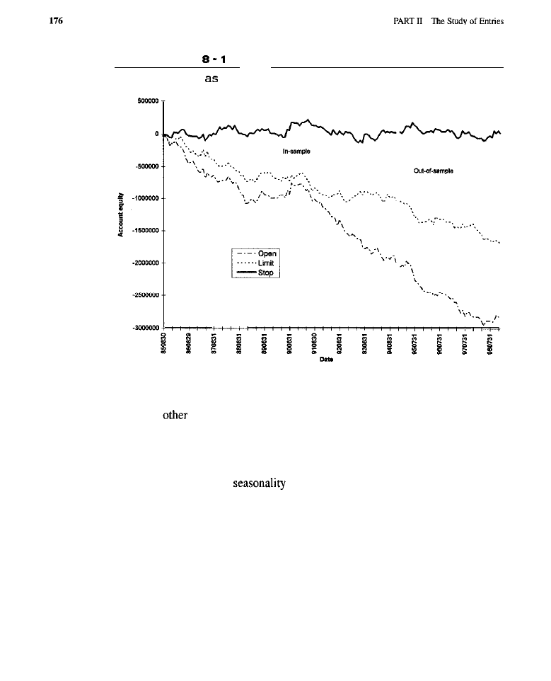
F I G U R E
Equity Growth
a Function of Order Type
started out the best, but after 1990, performance deteriorated. However, the equity
trend seemed to reverse to the upside after 1995 in the out-of-sample period, a time
when the
models tended to have declining equity when considered across all
order types.
CONCLUSION
These explorations into
have demonstrated that there are significant
seasonal effects to be found in the markets. Decisions about how to trade can be
made based on an examination of the behavior of the market at nearby dates for a
number of years in the past. The information contained on the same date (or a date
before or a date after) for a number of years in the past is useful in making a deter-
mination about what the market will do in the near future. Although the seasonal
effect is not sufficient to be really tradable on the whole portfolio, it is sufficient
to overcome transaction costs leading to some profits. For specific markets, how-
ever, even the simple models tested might be worth trading. In other words, sea-
sonal phenomena appear to be real and able to provide useful information. There
are times of the year when a market rises and times of the year when a market falls,
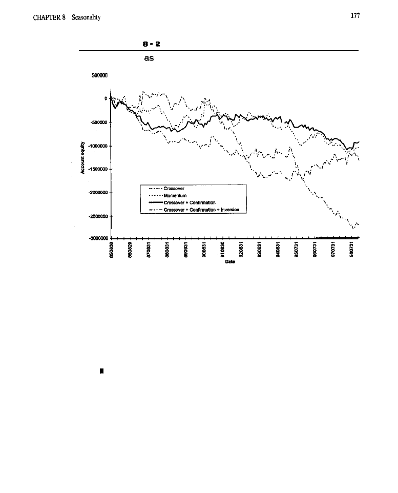
F I G U R E
Equity Growth
a Function of Model
and models like those tested in the chapter can capture such seasonal ebbs and
flows in a potentially profitable manner.
Seasonality, as defined herein, has been demonstrated to be worthy of seri-
ous consideration. If the kinds of simple entry models illustrated above are elabo-
rated by adding confirmations and by using an exit better than the standard one,
some impressive trading results are likely to result.
WHAT HAVE WE LEARNED?
Recurrent seasonal patterns appear to have real predictive validity and are
definitely worthy of further study.
n
The usefulness of seasonal patterns for trading varies from market to
market, with
certain
markets being particularly amenable to seasonal trad-
ing. Trading a basket of seasonally reactive markets could be a highly
lucrative endeavor.
n
To obtain the best results, raw seasonal information should be combined
with some form of confirmation or trend detection. Making use of additional
information can improve the performance of an unadorned seasonal model.

C H A P T E R
Lunar and Solar Rhythms
n the previous chapter, seasonal rhythms were defined as recurrent phenomena
connected to the calendar. Seasonality involves the orbital position and tilt of the
earth in relation to the sun. Every year, on approximately the same date, the earth
reaches a similar phase in its movement around the sun. Other solar bodies gener-
ate similar rhythms, most notably the moon, with its recurrent phases, and
“sunspot” phenomena. In this chapter, market cycles determined by external forces
will again be analyzed, but this time the relationship between market behavior and
planetary and solar rhythms will be examined.
LEGITIMACY OR LUNACY?
Discussion of planetary influences conjures up images of what some regard as
astrological nonsense. However, it seems arrogant to dismiss, a
the’possible
of lunar, solar, and other such forces, simply because of the pervasive
belief
that astrology (which Webster defines as “the pseudo-science which claims
to foretell the future by studying the supposed influence of the relative positions of
the moon, sun, and stars on human affairs”) is ludicrous. Such beliefs are often
based on the absence of knowledge. But what is already
known
about so-called
astrology, especially in the form of planetary and solar effects on earthly events?
Scientists have demonstrated some correlation between personality and plan-
etary positions. In one study (Mayo, White, and Eysenck,
published in the
Journal
of Social
Psychology, researchers tested the claim that introversion and
extroversion are determined by the zodiac sign a person is born under. A personal-
ity test was given to 2,324 individuals to determine whether they were introverts or
extroverts. The hypothesis was that individuals born under the signs Aries, Gemini,

Leo, Libra, Sagittarius, and Aquarius were likely to be extroverts, while those under
Taurus, Cancer, Virgo, Scorpio, Capricorn, and Pisces, tend to be introverts, The
results of the study were significantly consistent with the hypothesis, as well as
with other related studies (Gauquelin, Gauquelin, and Eysenck, 1979).
It is also known that the moon’s gravitational force influences the aquatic,
terrestrial, and atmospheric tides of the earth. The moon has been shown to affect
when coral spawn, when oysters open, when certain crimes are likely to be more
prevalent, and when “lunatics” (derived from the Latin word “luna,” which trans-
lates as “moon”) become more agitated. Moreover, women give birth and/or ovu-
late more frequently during
full moon.
When faced with the facts, the possibility of the moon influencing market
behavior is not so outlandish. Even Larry Williams (1979) found that the prices of
Silver, Wheat, Corn, and Soybean Oil rally when the moon is full and drop when
the moon is new!
Every amateur radio operator knows, “sunspots” exert a major influence on
long distance radio transmission. Sunspots appear as dark spots on
surface of
the sun. One theory is that they are produced by peculiarities in the gravitational
influences of neighboring planets on the Sun’s tidal rhythms. Another theory
explains sunspots as due to shifts in the sun’s magnetic poles. During high sunspot
activity, “skip” occurs: Short wavelength radio transmissions, which normally
carry only as far as line-of-sight, bounce off the ionosphere and may span dis-
tances of up to several thousand miles. Many have experienced this phenomenon
when watching television: A signal from a distant station will appear superim-
posed on a local one. Conversely, during low solar activity, long distance commu-
nication is much less likely at short wavelengths; anyone trying to achieve “DX”
(long distance communications), will need longer wavelengths.
Sunspot activity and solar flares are also correlated with terrestrial magnetic
storms that can disrupt sensitive electronics equipment and even knock out power
grids. Magnetic storms induced by solar eruptions in March I989 shut down the
power system, blacking out parts of Montreal and Quebec for up
to nine hours (Space Science Institute, 1996).
Changes in solar activity are even suspected of causing major fluctuations in
the earth’s climate, as when the “Little Ice Age” occurred in the
after 100
years of attenuated solar activity (Center for Solar and Space Research, 1997).
More relevant to traders: Edward R. Dewey, who established the Foundation
for the Study of Cycles in 1940, believed that there was a relationship between
sunspots and industrial production. Perhaps such a relationship is mediated by
matological effects on agriculture, making it worthwhile to examine the correla-
tion between solar activity and agricultural commodity prices.
Our interest in sunspots peaked upon noticing that, during 1987, there
were only three days when the sunspot number (an index of solar activity) was
greater than 100. Two of those days were October 15 and
The probability

of the correspondence between Black Monday and heightened solar activity is
less than one in 100.
In the section below on “Lunar Cycles and Trading,” the impact of the lunar
phase on prices is examined. The impact of solar activity is examined in “Sunspots
and Market Activity.”
LUNAR CYCLES AND TRADING
In a previous study (Katz and McCormick, June
we found that lunar cycles
could be used to profitably trade the NYFE. From 1990 to 1997, a simple lunar
system produced a net profit of $75,550. There were 170 trades, 60% profitable.
The average one contract trade made $444.41; the return-on-account was 365%
(not annualized). The long side performed better (520%) than the short (-37%).
The signals often marked turning points to the very day. Silver also responded
well, with signals picking off exact tops and bottoms; both longs and shorts were
profitable with a 190% return over the same period as for the NYFE. Even Wheat
traded profitably long and short with a 242% return. Given only one parameter (a
displacement in days since the full or new moon), and many trades, the results are
impressive and probably robust.
Our results were encouraging enough to justify further study of entries based
on these phenomena. The study will involve the phases of tbe moon, i.e., full
moon,
quarter, last quarter, new moon, and
phases in between. Can the
lunar phase predict whether the market is bottoming or topping? Do bottoms (or
tops) form at the time of the full moon, or perhaps
days before the full moon,
or at the new moon? Since the lunar cycle may affect different markets differently,
the adaptive approach taken with
is again used.
GENERATING LUNAR ENTRIES
There are many ways to time entries based on the lunar rhythm. Two approach-
es are employed in the tests: momentum and crossover. To calculate momentum,
a series of price changes is computed and then a
centered smoothing
(one that
induces no delays or phase shifts) is applied. For normalization, each price
change in the smoothed series is divided by the
average true range. For
each bar, we ask: “What phase is the moon in currently?” As many past instances
as possible are found in which the moon was in the identical phase and the
momentum of prices on the corresponding bars is examined. The average of the
momentums becomes the value placed in the lunar
series, which
reflects the expected rate-of-change (momentum) in prices at a given time based
on historical price movement at the phase of the moon existing on the current
bar. Each number in the lunar momentum series is determined only by events
about 27 or more days ago; this is why centered smoothing, and other techniques
that look ahead in time relative to any specified bar, are permissible. Entries are
taken when momentum crosses above a positive threshold (a buy signal is
issued), or when momentum crosses below a negative threshold (a sell is post-
ed). Buying or selling can take place at the open, on a limit, or on a stop. The
momentum calculations and generation of entries closely follow those for
but, instead of looking to previous instances of the same date in earlier
years, previous instances of the moon having a phase identical to that on the tar-
get bar are examined.
Entries can also be generated by computing the price differences, normaliz-
ing them, and integrating the series to obtain a pseudo-price series based on pre-
vious instances of the correct lunar phase. A moving average crossover model is
then applied to that series. Because the value at any bar in the series is determined
only by bars roughly 27 or more days ago, the delay in the crossovers can be com-
pensated for by looking ahead a small number of bars.
Both methods are
in that no specific information is required
about the phase of the moon on which to place a buy or sell order. The adaptive
quality is important because different markets respond to the moon differently,
as seen in our earlier study. Both methods differ from the previous research,
where buys or sells occurred a
number of days before or after a full or a
new moon.
Several rules for handling confirmations and inversions are also tested to
determine whether better results can be obtained over the basic models. An exam-
ple of
is the following: If a buy signal occurs on a given bar and
everything behaves as expected, the market should bottom around the time of the
buy; if instead it tops, the buy signal might be suspect, i.e., the market may not
be adhering to its typical seasonal or lunar timing. The
model implements the crossover model with an additional
that must be
satisfied before a buy or sell can be issued. a buy signal occurs, the Slow %K
on the signal bar must be less than
meaning the market is near the bottom
of its recent historical range. Likewise, if the model generates a sell signal, a
check is made to see whether Slow %K is greater than
indicating that the
market is near the top of its range, as would be expected if it is responding to
lunar influence. The
and
inversion
model
adds another element: If
a buy is signalled, and the market is near the top of its range (Slow %K greater
than
then an inversion is assumed and, instead of issuing a buy, a sell order
is posted. If a sell is signalled, but the market is near the bottom of its recent
range, a buy order is issued.
The characteristics of lunar entries are similar to seasonal entries: Both are
predictive, rather than responsive, and thus lend themselves to countertrend trad-
ing. And, as with any predictive entry, they may be out of tune with market behav-
ior. As with seasonal entries, cycle or rhythm inversions may occur.

LUNAR
METHODOLOGY
All tests were performed using lunar entries to trade a diversified portfolio. Can
lunar entry models result in profitable trades? How have such models fared over
time? Have they become more or less profitable in recent years? The tests will
address these questions.
The exits are the standard ones. Entry rules are discussed when presenting
individual tests. Trades are closed out when either an entry in the opposing direc-
tion takes place, or when the standard exit closes the trade, whichever comes first.
The following code implements the lunar-based entry models that underlie all tests.

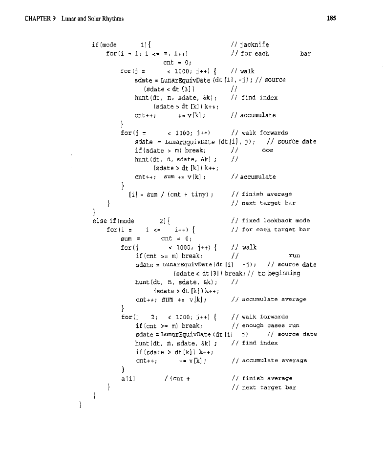
= =
mode
(
t a r g e t
sum = 0.0;
2; j
backwards
d a t e
i f
b r e a k ;
run to beginning
i f
sum
a v e r a g e
2; j
(
avoid
d a t a
f i n d i n d e x
i f
a v e r a g e
a
= =
1;
n;
0.0;
= 2; j
,
i
f
i f
=
j
,
sum
= s u m
t i n y )
backwards
enough cases
r u n
find index

static void
float
float
float
float
float
float
float
Implements a variety of lunar-cycle trading models.
=
vector
of parameters
in
vector
of opening prices
hi
of high prices
prices
vector
of closing prices
open interest numbers
vector
of average dollar
of bars in data series or vectors
trading simulator class instance
vector
equity
static
signal;
static
static float
limprice,
thresh;
static float
,
static
static float
copy parameters
local variables for clearer reference
length of moving
displacement factor
threshold for
models
=
average type:
moving average
simple
exponential
triangular
type:
with confirm
with confirm and inversions
=
entry:
maximum holding period

ptlim
4;
profit target in volatility
loss in volatility units
Perform whale-series computations that are unaffected by
any parameter*.
may
saved in
dramatically reducing execution time.
if
==
= vector
,
h i ,
= 0.0;
= 2;
=
-2.0,
market index
allocated
table
table
vector
price change
normalization
clipping
seasonal
progress
perform other whole-series computations
(
1:
series for momentum model
smoothing
=
ma*, 1,
deviation
break;
case 2:
3:
4:
series for
models
2;
nb;
integration
smoothing
3
stochastic
break;
default:
invalid


189

Several functions required to calculate lunar rhythms for any market in an
adaptive manner precede the code implementing the trading model. The imple-
mentation function,
Model,
follows the standard conventions: After declarations,
parameters are copied into local variables for easier reference. Comments indicate
what the parameters control. The
block computes the
average true
range
used in the exits and for normalization, as well as the lunar sea-
sonal series
the predicted price changes for each bar. These series are
computed only once for each market and tabled; this may be done as no relevant
parameters change from test to test as
Model
is repeatedly called. A second block
calculates the model-specific time series needed to generate entry signals. If
is the simple momentum model is used; 2 = the crossover model; 3 =
crossover with confirmation; and 4 = crossover with confirmation and inversion.
Among the series that may be computed are: smoothed lunar momentum, integrat-
ed lunar momentum (price-like series), moving averages for the crossover model,
and Slow %K for models involving
and inversion. Depending on
several other parameters may become important. One parameter,
controls the length of all moving averages: For the momentum model, it
controls the length of the centered triangular moving average; and for the crossover
models, it controls the length of the two moving averages those models require.
Another parameter,
sets the displacement: This is the look-ahead used, e.g., to
compensate for the lag of the moving averages. The parameter
thresh
is the thresh-
old used in the momentum model for both short and long trades (short trades use
the negative of thresh). Variable
controls the type of certain moving aver-
ages: 1 = simple, 2 = exponential, 6 = centered exponential, 7 = centered trian-
gular; other moving averages are available, but are not used in the analyses. After
all series are calculated, a loop is entered that steps, day by day, through the mar-
ket to simulate trading. This loop contains code to update the simulator, determine
the number of contracts, avoid trading on limit-locked days, etc. The next block,
appearing within the bat-stepping loop, generates entry signals. The rules are deter-
mined by
Finally, a block handles posting the appropriate trading order,
as selected by the
1 = entry at open, 2 = on limit, 3 = on stop.
LUNAR TEST RESULTS
Tests were run on four
models: crossover, momentum, crossover with
and crossover with confirmation and inversions. Each model
studied
with entry at
on limit, and on stop. Table 9-l summarizes the results of all tests,
broken down by sample, entry order, and model. For each model, there is a row of
numbers containing the annualized portfolio return, and a row with the average port-
folio dollar profit or loss per trade. Averages across all order types for in-sample and
out-of-sample performance are in the two rightmost columns. The last two rows con-
tain the average across models for each type of order.

Tables 9-2 and 9-3 present information for each of the 12 tests on the spe-
cific commodities that the model traded profitably and those
lost, for the
sample (Table 9-2) and out-of-sample (Table 9-3) runs. The first column,
SYM,
is
the market being studied. The last column
is the number of profitable
tests for a given market. The numbers in the first row are Test identifiers. The last
row
contains the number of markets profitable for a given model. Tables
9-2 and 9-3 provide information about which markets are and are not profitable
when traded by each model: One dash indicates a loss per trade of $2,000 to
$4,000; two dashes represent a loss of $4,000 or more; one plus sign (+)
means a profit per trade of $1,000 to $2,000; two pluses (+ indicate gains of
more; a blank cell means a loss between $0 and $1,999 or a profit
between $0 and $1,000 per trade.
Tests of the Basic Crossover Model
A moving average
was computed for the integrated, price-lie lunar series. A
second moving average
was taken of the first moving average. A buy signal
was generated when
ml
crossed above
A sell signal was generated when
crossed below
This is the same moving average crossover model discussed in
the chapter on moving averages, except here it is computed on a lunar series, rather
than on prices. The entries were effected by either a market at open (Test
a limit
(Test
or a stop order (Test 3).
Optimization involved stepping the length of the moving averages
from 5 to 15 in increments of and the displacement
from 0 to in
Performance of Lunar Models Broken Down by Model, Order, and
Sample
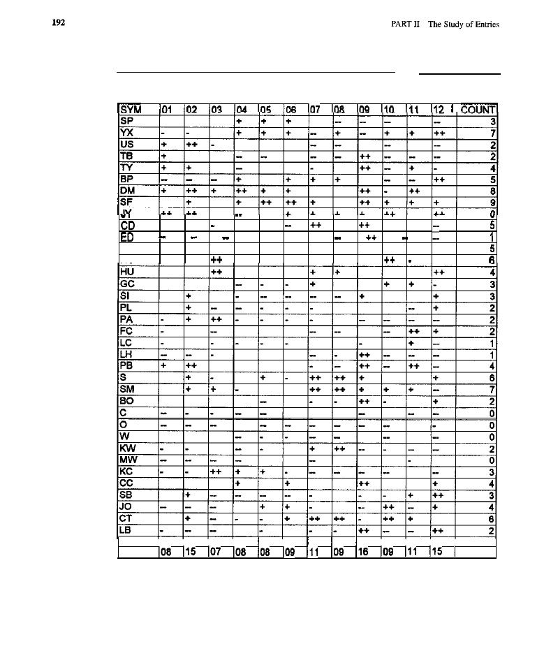
T A B L E
S - 2
In-Sample Performance Broken Down by Test and Market
+ l +
++
__ __
CL + + ++ +
+
HO
+
++ +
++
I
I
COUNT

T A B L E S - 3
Out-of-Sample Performance Broken Down by Test and Market

ments of 1. For entry at the open, the best performance (in terms of in-sample
risk-to-reward ratio) was achieved with a moving average length of 15 and a dis-
placement of 8: entry on a limit was best with a length of 15 and a displacement
of 6; entry on a stop required a length of 15 and a displacement of 12.
No tests showed profits in either sample. In-sample, best performance (least
average loss per trade) was with entry on limit; entry on stop produced poorer
results; entry at open was the worst. With the limit order, 43% of the 1,759 trades
were profitable. Out-of-sample, the limit order produced the smallest average loss
per trade and the stop yielded the largest loss. Overall, the system did not do well
on the entire portfolio. The relative performance of shorts and longs was incon-
sistent across orders and samples. In-sample, longs lost substantially more than
shorts, the opposite of what was frequently seen in tests of other models.
Equity steadily declined from the beginning to the end of the data series for
entry at open. For entry on limit, equity was choppy but up, peaking in September
1989. then declined until July 1992, rose slightly until February 1994, and
declined steadily until July 1998, when it suddenly began increasing. With a stop,
equity showed a choppy decline from one end of the data series to the other.
In-sample, the number of markets with positive returns using a limit, a
market-at-open, and a stop were 15, 8, and 7, respectively. Out-of-sample, the
limit produced the best results
followed by the market-at-open
and
the stop (14). More market-order combinations produced profits out-of-sample
than in-sample; it seems that many markets are becoming more affected by lunar
rhythms in recent years. In-sample, only the Deutschemark and Light Crude
were profitable across all three entry orders. Out-of-sample, the Deutschemark
was highly
with limit and stop orders; Light Crude slightly lost with
the stop. T-Bonds strongly profitable in both samples with the limit. Pork Bellies
was profitable in both samples with entry at open and on limit. Considering only
the limit order, profit in both samples was observed for the Deutschemark, Swiss
Franc, Japanese Yen, Platinum, Palladium, Sugar, and Cotton.
Tests of the Basic Momentum Model
A centered moving average smoothed the unintegrated lunar price change series.
No lag was induced because the centered average examines as many future (rela-
tive to the current bar), as it does past, data points. This smoothing is legitimate
because, in the calculations, the lunar estimate at the current bar involves data at
least two lunar cycles (about two months) away. For the smoothed lunar price
changes, a series of average absolute deviations was computed and a
sim-
ple moving average was taken to produce the desired result. A buy was issued
when lunar momentum, at the current bar plus some displacement
was
greater than some multiple (thresh) of the average absolute deviation of the lunar
momentum. A sell was issued when lunar momentum, at the same displaced bar,

was less than minus the same multiple of the average absolute deviation. Entries
were executed at the open (Test
on a limit (Test
or on a stop (Test 6).
Optimization was for the length of the moving averages (stepped from 5 to
15 in increments of the displacement (1 to 10 in steps of and the threshold
(1.5 to 2.5 in steps of 0.5). Best results were achieved with the length, displace-
ment, and threshold parameters set to 10, 10, 2 for the market-at-open and 15, 9,
1.5 for the limit and stop.
Overall, results were worse than for the crossover model. Heavy losses
occurred in both samples across all order types. The same poor performance was
observed when seasonal effects were analyzed with the momentum model. Longs
again performed better than shorts.
With entry at open, portfolio equity declined smoothly and severely, with the
rate of loss gradually decreasing over time. With a limit order, equity steadily
decreased. With a stop, equity dropped sharply from the beginning of the sample
until August 1988, then declined gradually.
In-sample, the S&P 500, NYFE, Deutschemark, and Swiss Franc were
somewhat profitable across all orders. Out-of-sample, the S&P 500 and NYFE
neither profited nor lost, but the Deutschemark did well with entry at open, and the
Swiss Franc with entry on limit and on stop. As with the crossover model, there
were many more profitable market-order combinations.
Tests of the Crossover Model with Confirmation
This is identical to the basic crossover model except that entries were only taken
when an appropriate reading of the Fast %K Stochastic confirmed lunar market
behavior. Specifically, if the lunar crossover suggested a buy, it was only acted
upon if Fast
was below 25%; before a buy occurred, the market had to be
down or near a bottom, as expected on the basis of the lunar rhythm. Likewise, a
lunar sell was not taken unless the market was near a possible top, i.e., Fast
greater than 75%. Entries were at the open, on a limit, or a stop (Tests 4 to 6,
respectively).
The length of the moving averages
was optimized from 3 to IS in
increments of 3, and displacement
from 0 to 15 in increments of 1. Best per-
formance was achieved for entry at the open, and on a limit, with a moving aver-
age length of 15 and a displacement of 12; the best stop entry occurred with a
length of 12 and a displacement of 5.
In-sample, the results were somewhat better than the basic crossover model:
When combined with the stop, the crossover with confirmation yielded about $234
per trade. Out-of-sample, however, the average
was more than for either of the
previous two models, regardless of order. The stop showed the smallest loss per
trade and was best. This is another system not profitable on a whole portfolio
basis. The equity curves showed nothing but losses across all three orders.

In-sample, the
Heating Oil, Soybeans, and Soybean Meal were
profitable with all three orders; out-of-sample, only losses or, at best, unprofitable
trading occurred in these markets. Kansas Wheat showed consistent behavior
across samples: Results were profitable with entry at open and on limit, and
unprofitable with entry on stop. Across samples, the British Pound and Swiss
Franc were profitable, as was the Canadian Dollar, Eurodollar, and Pork Bellies
with entry on a stop. Since the number of trades was fairly small for
mar-
kets and
whole portfolio, results are probably not trustworthy.
Tests of the Crossover Model with Confirmation
and Inversions
This is the same as the crossover model with confirmation, but additional trades
were taken at possible inversions. If a lunar buy was signalled by a crossover,
but the market was high (Fast %K being greater than
a sell (not a buy) was
posted; the assumption is the usual lunar cycle may have inverted, forming a top
instead of a bottom. Likewise, if the crossover signalled a sell, but the market
was down, a buy was issued. These signals were posted in addition to those
described in the crossover with confirmation model. Entries occurred at the open
(Test
on a limit (Test
or a stop (Test 12).
The length of the moving averages
was stepped from 3 to 15 in
increments of 3, and the displacement
from 0 to 15 in increments of 1. For
entry at the open, the best moving average length was 15 and displacement, 12;
entry on a limit was best with a length of 15 and a displacement of 8; entry on a
stop required a length of 12 and displacement of 15.
This model lost heavily across samples and orders. As with seasonality,
inversions did not benefit performance. The equity curve paints a dismal picture.
In-sample, the NYFE was profitable across all three orders, but
S&P 500
lost for two of the orders and was flat for the
The Swiss Franc was also prof-
itable in-sample across all three orders; out-of-sample, it was very profitable for
entry at open, but lost for
other two orders. There was a great deal of incon-
sistency in results between the samples.
SUMMARY ANALYSES
When considered over all models, the stop performed best in both samples. The
worst performers were, in-sample, the open and, out-of-sample, the limit. In-sample,
when considered over all order types, crossover with
was the best.
of-sample, the basic lunar crossover model performed best and crossover with
worst.
There were many strong interactions between sample, model, and order. Some
of the results stem from the small number of trades. The best of the seasonal

order combinations yielded better and more consistent performance than the best of
lunar ones.
CONCLUSION
When entire portfolios are considered, entry models based on lunar rhythms do
not do as well as those based on seasonal rhythms. The poor showing of the lunar
effect contradicts
earlier study (Katz and McCormick, June 1997). The differ-
ences may stem from two possible factors: entry models and exits. In the current
tests, the models were optimized on an entire portfolio, which may not be appro-
priate for the lunar rhythm (the earlier model entered the market a specified num-
ber of days after full or new moon). The methods used in this chapter were altered
from the previous study because of the need to optimize using common parame-
ters across all markets. Doing this with the earlier approach would require that
trades be entered n-days after the full or new moon, regardless of the market being
traded; since lunar rhythms are distinct for each market (as demonstrated in our
previous study), this approach was inappropriate. The earlier model was, there-
fore, redesigned to be self-adaptive, i.e., as it proceeds through lunar cycles, the
appropriate timing for trading is decided by analysis of previous lunar cycles.
Another possible reason for the conflicting results may be the interaction
between the exits and entries, The lunar model, and perhaps the seasonal model,
has the property of pinpointing tradeable tops and bottoms, but only a percentage
of the time. Such systems work best with very tight stops that quickly cut losses
when predictions go wrong, but that allow profits to accumulate when correct.
In general, the lunar models performed poorly, but there were individual mar-
kets with consistent, positive performance-encouraging, given the model was not
optimized to them. Results suggest that some great systems are hiding here if
entries were tailored to them, e.g., in our earlier study, the lunar model traded Silver
well; in the current study, Silver was not strongly responsive. Although the lunar
models lost money on the portfolio, they lost very much less on a per-trade basis
than did, for instance, most moving average and oscillator entry models.
SOLAR ACTIVITY AND TRADING
An earlier study (Katz and McCormick, September 1997) examined the effects of
sunspots on the S&P 500 and Wheat. In-sample, a simple sunspot model pulled
$64,000 from the S&P 500 between 1984 and 1992. There were 67 trades, 31%
profitable. The average winning trade was
much larger than the average
loser
The average trade was $955.22 with a return of 561% (not annu-
alized). The long side was profitable, but the short side was substantially more so,
highlighting the tendency of unusual solar activity to coincide with market crashes.
The better performance of short trades is especially significant, since this market

was in a secular
during most of the testing period. Profitability continued
out-of-sample, from 1993 through 1996, with a 265% return, 23 trades (30% prof-
itable), and with an average trade yielding $891.30. The results for Wheat were also
good across samples. In-sample, 57% of X4 trades were profitable with a $203.27
average trade and 859% return (not annualized). Out-of-sample, there were 29
trades, 55% profitable, a $260.78 average trade, and 406% return.
Our initial research suggested further study would be worthwhile. The tests
below examine the effects of solar activity on the
standard
portfolio. Daily sunspot
numbers from 1985 through 1999, from the Royal Observatory of Belgium, were
used to generate entries.
G E N E R A T I N G S O L A R E N T R I E S
There are many ways to generate entries
based
on solar activity. The method used
below is a simple variation of a breakout model, applied to sunspot counts, not prices.
The rules are: If the current sunspot number is higher than the
upper thresh-
old, and the sunspot counts for a certain number
of previous bars were lower
than their corresponding thresholds, then either a buy or sell signal (depending on
previous market behavior in response to upside breakouts in the sunspot numbers) is
issued. If the current sunspot number is lower than the current lower threshold, and
the sunspot counts for
same number of previous bars were
higher than their
corresponding thresholds, then either a sell or a buy signal (again, depending
on
pre-
vious market behavior) is issued. The signals are not responded to immediately, but
only after a specified number of days
The breakout thresholds are determined
as follows: The upper threshold, used for a given bar, is the highest sunspot number
found in a certain larger number of previous bars
while the lower threshold is
set at tbe lowest of the sunspot numbers in those previous bars. “Previous market
behavior” refers to whether the market was near the bottom or top of its near-future
range when a
kind of breakout occurred. If a given direction of solar
out is historically associated with the market being near the bottom of its near-future
range, a buy signal is generated, on the other hand, if the market is characteristically
near the top of its near-future range, a sell signal is generated.
Like lunar phenomena and seasonality, entries based on solar activity share
the assumption that market behavior
is
by external factors and that the
independent, influential variable has predictive value, i.e., market behavior is
anticipated rather than responded to. As with any predictive system, the forecasts
may be more or less correct. Trades resulting from incorrect predictions can be
incredibly bad, even if many trades resulting from correct predictions are perfect,
as is often the case with predictive systems. Being anticipatory, the models lend
themselves to countertrend entries, which means better tills, less slippage, and bet-
ter risk control, assuming appropriate stops are used (not done here because of the
need to maintain the standard exit).
199
The code for these tests is similar to that for lunar analysis and so is not pre-
sented here. It is available on the companion software CD (see offer at back of
book).
SOLAR TEST RESULTS
Tests were performed on the solar entry model using entry at open (Test on a
limit (Test and on a stop (Test 3). The breakout look-back
was stepped
from 25 to 40 in increments of 5; the repeat prevention look-back
from
to
15 by 5; and the displacement
from 0 to 2 by 1. For entry at the open, the
best in-sample performance was with a breakout look-back of 35, a repeat pre-
vention look-back of 15, and a displacement of 2. For the limit, a breakout
back of 40, a repeat prevention look-back of 15, and a displacement of 0 were
optimal. For the stop, the best values were: for the breakout look-back, 35; for the
repeat prevention look-back, 15; and for the displacement, 2.
Table 9-4 shows both the in- and out-of-sample performance for
commodities. The columns and rows contain the same kinds of data as in Tables
9-2 and 9-3 above.
The solar model performed about as well as the lunar ones and, in sample,
did best with a stop order. In-sample, entry at the open was worst
per
trade); a limit was slightly better
substantially so when only long trades
were considered. The stop order was the best, losing only $52 per trade; were it
not for transaction costs, this order would have been very profitable in-sample.
The mode1 required the theoretically expected displacement. The best dis-
placement for the limit was zero, understandable since the goal is to respond
quickly, before the market turns, when a limit can enter on the noise. With the stop,
a displacement of 2 was best: Movement needs to begin to trigger the stop and
cause entry. The average loss per trade worsened, from
to
when dis-
placement deviated just one or two bars from its optimal value. This implies a rela-
tionship between the timing of the market and solar events otherwise small
changes in the displacement should have little or no effect.
With the stop order, the highest percentage of wins (in-sample) was obtained
and the long side was actually profitable. Out-of-sample, the stop was again best,
but the average loss per trade was a substantial $1,329.
Equity was examined only for the stop, since the other orders performed so
poorly. Equity rose very rapidly until June 1988, then, until October 1990, it was
choppy and fairly flat. Between October 1990 and June 1994, equity declined
sharply, then was choppy and slightly down.
Interestingly, some of our previous findings (Katz and McCormick,
September 1997) were confirmed. With the stop, which generally performed best
on the whole portfolio, the S&P 500 was very profitable in both samples. The
average trade returned $4,991 in-sample: the return was 20.4% annualized; and,

200
T A B L E B - 4
Broken
Down
by Sample, Test, and Market
SYM
Count
I
I I
I
II

the t-test indicated a greater
80% probability that the effect was real and
would hold up. Both long and short trades were profitable. In-sample there were
37 trades (40% winners). Out-of-sample, longs and shorts both continued to be
profitable; it was surprising that the shorts were profitable because the market was
in a steep up-trend during most of that period. Out-of-sample, the return was
39.5% annualized, with an 80% probability of being real; there were 11 trades
(45% winners), and the average trade returned $5,640. These are excellent results.
The observation that sharp down-turns can occur after solar flares has been
supported. With
stop order, Minnesota Wheat, Soybeans, and Cotton were also
profitable in both samples. Minnesota Wheat pulled 13.5% annually in-sample,
again with a better than 80% chance of the results being real, and 30.5%
sample, with almost an 85% probability of the effect not being due to chance.
Interestingly, Light
and Heating Oil were highly profitable in-sample, but
lost moderately out-of-sample. There were a few profits in other markets, but no
consistency between in- and out-of-sample performance with the stop.
CONCLUSION
Like seasonality and lunar phase, solar activity appears to have a real influence on
some markets, especially the S&P 500 and Minnesota Wheat. As with lunar
cycles, this influence is not
strong or reliable to be a primary element
in a portfolio trading system; however, as a component in a system incorporating
other factors, or as a system used to trade specific markets, solar activity is worth
attention. We personally do not believe solar influences directly determine the
market. We do suspect that they act as triggers for events that are predisposed to
occur, or as synchronizers of already-present market rhythms
similar
For example, if a market is highly over-valued and unstable, as was the
S&P 500 in October 1987, a large solar flare might be sufficient to trigger an
already-imminent crash.
WHAT HAVE WE LEARNED?
. Lunar and solar phenomena may have real impact on commodities mar-
kets. In the case of solar phenomena, such impact on the S&P 500 has
been
With lunar phenomena, there is more inconsistency in
the results, but influence is clearly detectable.
n
The phenomena are probably worth including in a more elaborate trading
model, e.g., as inputs to a neural network.
n
Models that capture such influences almost certainly need to be tuned to
specific markets in a more effective way
has been done here. Such
market specificity might be the reason for the better results observed
when tests were conducted on individual markets.

. As with other countertrend models that pinpoint turning points (including
seasonality), it is probably necessary to use an exit that includes a fairly
tight stop. If a turning point is correctly identified, the stop is never hit
and the trade quickly turns profitable. On the other hand, when predic-
tion error occurs, as frequently happens, the stop quickly kills the trade,
cutting losses short. The use of tight stops may be another factor that
accounts for better performance in our earlier studies (Katz and
McCormick, June and September 1997) than in the current tests.
. Given the highly probable influence of
and lunar rhythms on certain
markets, it might be worth exploring some other planetary rhythms,
including the kinds of planetary configurations and cycles that are the
focus of astrologers.
. Entry orders interact with models. Limit orders, for example, do not
always perform best. It seems a stop order sometimes improves perfor-
mance. The reason may be that a stop order introduces verification of the
beginning of a trend before entry can occur, something that may be
important when using a prediction-based counter-trend strategy.

C H A P T E R 1 0
Cycle-Based Entries
A
cycle
is a rhythmic oscillation that has an identifiable frequency (e.g., 0.1
cycle per day) or, equivalently, periodicity (e.g., days per cycle). In the previ-
ous two chapters, phenomena that are cyclic in nature were discussed. Those
cycles were exogenous in origin and of a known, if not fixed, periodicity.
Seasonality, one such form of cyclic phenomena, is induced by the periodicity and
recurrence of the seasons and, therefore, is tied into an external driving force.
However, while all seasonality is cyclic, not all cycles are seasonal.
In this chapter, cycles that can be detected in price data alone, and that do not
necessarily have any external driving source, are considered. Some of these cycles
may be due to as yet unidentified influences, Others may result only from reso-
nances in the markets. Whatever their source, these are the kinds of cycles that
almost every trader has seen when examining charts. In the old days, a trader
would take a comb-like instrument, place it on a chart, and look for bottoms and
tops occurring with regular intervals between them. The older techniques have
now been made part of modem, computerized charting programs, making it easy
to visually analyze cycles. When it comes to the mechanical detection and analy-
sis of cycles,
spectral analysis (MESA) has become the preem-
inent technique.
CYCLE DETECTION USING MESA
Currently, there are at least three major software products for traders that employ the
maximum entropy method for the analysis of market cycles: Cycle Trader
and
(Scientific Consultant Services,
516-696-3333, and Ruggiero Associates, 800-21 l-9785). This kind of analysis has

been found useful by many market technicians. For example,
(October
1996) contends that adaptive breakout systems that make use of the maximum
entropy method (MEM) of cycle analysis perform better than those that do not.
Maximum
entropy is an elegant and efficient way to determine cyclic activity
in a time series, Its particular strength is its ability to detect sharp spectral features
with small amounts of data, a desirable characteristic when it comes to analyzing
market cycles. The technique has been extensively studied, and implementations
using maximum entropy have become polished relative to appropriate preprocess-
ing and postprocessing of the data, as required when using that algorithm.
A number of problems, however, exist with the maximum entropy method,
as well as with many other mathematical methods for determining cycles. MEM,
for example, is somewhat finicky. It can be extremely sensitive to small changes
in the data or in such parameters as the number of poles and the look-back period.
In addition, the price data must not only be de-trended or
but also be
passed through a low-pass filter for smoothing before the data can be handed to
the maximum entropy algorithm; the algorithm does not work very well on noisy,
raw data. The problem with passing the data through a filter, prior to the maximum
entropy cycle extraction, is that lag and phase shifts are induced. Consequently,
extrapolations of the cycles detected can be incorrect in terms of phase and timing
unless additional analyses are employed.
DETECTING CYCLES USING FILTER BANKS
For a long time, we have been seeking a method other than maximum entropy to
detect and extract useful information about cycles. Besides avoiding some of the
problems associated with maximum entropy, the use of a novel approach was also
a goal: When dealing with the markets, techniques that are novel sometimes work
better simply because they are different from methods used by other traders. One
such approach to detecting cycles uses banks of specially designed band-pass fil-
ters. This is a method encountered in electronics engineering, where
banks
are often used for spectral analysis. The use of a filter bank approach allows the
bandwidth, and
filter characteristics, to be tailored, along with the overlap
between successive filters in the bank. This technique helps yield an effective,
adaptive response to the markets.
A study we conducted using filter banks to explore market cycles produced
profitable results (Katz and McCormick, May 1997). Between January 3, 1990,
and November 1, 1996, a filter bank trading model, designed to buy and sell on
cycle tops and bottoms, pulled $114,950 out of the S&P
There were 204
trades, of which 50% were profitable. The return-on-account was 651% (not annu-
alized). Both the long and short sides had roughly equal profitability and a similar
percentage of winning trades. Various parameters of the model had been opti-
mized, but almost all parameter values tested yielded profitable results. The

meters determined on the S&P 500 were used in a test of the model on the T-Bonds
without any changes in the parameters, this market also traded profitably,
ing a 254% profit. Given
relative crudeness of the filters used, these results
were very encouraging.
In that study, the goal was simply to design a zero-lag filtering system. The
filters were analogous to resonators or tuned circuits that allow signals of certain
frequencies (those in the pass-band) to pass through unimpeded, while stopping
signals of other frequencies (those in the stop-band). To understand the concept of
think of the stream of prices from the market as analogous to the elec-
trical voltage fluctuations streaming down the cable from an aerial on their way to
a radio receiver. The stream of activity contains noise (background noise or “hiss”
and static), as well as strong signals (modulated cycles) produced by local radio
stations. When the receiver is tuned across the band, a filter’s resonant or center
frequency is adjusted. In many spots on the band, no signals are heard, only stat-
ic or noise. This means that there are no strong signals, of the frequency to which
the receiver is tuned, to excite the resonator. Other regions on the band have weak
signals present, and when still other frequencies are tuned in, strong, clear broad-
casts are heard; i.e., the filter’s center (or resonant frequency) corresponds to the
cyclic electrical activity generated by a strong station. What is heard at any spot
on the dial depends on whether the circuits in the radio are resonating with any-
thing, i.e., any signals coming in through the aerial that have the same frequency
as that to which the radio is tuned. If there are no signals at that frequency, then
the circuits are only randomly stimulated by noise. If the radio is tuned to a cer-
tain frequency and a strong signal comes in, the circuits resonate with a coherent
excitation. In this way, the radio
serves
as a
resonating filter
that may be tuned to
different frequencies by moving the dial across the band. When the filter receives
a signal that is approximately the same frequency as its resonant or center fre-
quency, it responds by producing sound (after demodulation). Traders try to look
for strong signals in the market, as others might look for strong signals using a
radio receiver, dialing through the different frequencies until a currently broad-
casting station-strong market cycle--comes in clearly.
To further explore the idea of resonance, consider a tuning fork, one with a
resonant frequency of 440 hertz (i.e., 440 cycles per second), that is in the same
room as an audio signal generator connected to a loud speaker. As the audio gen-
erator’s frequency is slowly increased from 401 hertz to 402 to 403, etc., the res-
onant frequency of the tuning fork is gradually approached. The nearer the audio
generator’s frequency gets to that of the tuning fork, the more the tuning fork
picks up the vibration from the speaker and begins to emit its tone, that is, to res-
onate with the audio generator’s output. When the exact center point of the fork’s
tuning (440 hertz) is reached, the fork oscillates in exact unison with the speak-
er’s cone; i.e., the correlation between the tuning fork and the speaker cone is per-
fect. As the frequency of the sound emitted from the speaker goes above (or

below) that of the tuning fork, the tuning fork still resonates, but it is slightly out
of synch with the speaker (phase
occurs) and the resonance is weaker. As
driving frequencies go further away from the resonant frequency of the tuning
fork, less and less signal is picked up and responded to by the fork. If a large
number of tuning forks (resonators or filters) are each tuned to a slightly differ-
ent frequency,
there is the potential to pick up a multitude of frequencies or
signals, or, in the case of
markets, cycles. A particular filter will resonate very
strongly to
cycle it is tuned to, while
other filters will not respond because
they are not tuned to the frequency of that cycle.
Cycles in the market may be construed in the same manner as described
above-as if they were audio tones
vary over time, sometimes stronger, some-
times weaker. Detecting market cycles may be attempted using a bank of filters
that overlap, but that are separate enough to enable one to be found that strongly
resonates with the cyclic activity dominant in the market at any given time. Some
of the filters will resonate with the current cyclic movement of the market, while
others will not because they are not tuned to the
of current
market activity. When a filter passes a signal that is approximately the same fre-
quency as the one to which it is tuned, the filter will behave like the tuning fork,
i.e., have zero lag (no phase shift); its output will be in synchrony with the cycle
in the market. In addition, the filter output will be fairly close to a perfect sine
wave and, therefore, easy to use in making trading decisions. The filter bank used
in our earlier study contained Butterworth band-pass filters, the code of which was
rather complex, but was fully disclosed in the Easy Language of
Filters
Butterworth filters are not
to understand. A low-pass
is
like a moving average: It both attenuates higher-frequency (shorter-periodicity)
signals (or noise) and passes lower-frequency (higher-periodicity) signals unim-
peded; in other words, it smooths data. While an exponential moving average has
a stop-band cutoff of 6 decibels (db) per
(halving of the output for every
halving of the signal’s period below the cutoff period), a
Butterworth filter
(the kind used in our May 1997 study) has a stop-band attenuation of 18 decibels
per octave (output drops by a factor of 8 for every halving of a signal’s period
below the cut-off period). The sharper attenuation of unwanted higher-frequency
(lower-periodicity) activity with
Butterworth filter comes at a price: greater lag
and distorting phase shifts.
A
high-pass
is like a moving-average difference oscillator
(e.g., X MA(X), where X is the input signal): Both attenuate lower-frequency sig-
nals (e.g., trend), while passing higher-frequency signals unimpeded. The attenua-
tion in the stop-band is sharper for the
filter (18 db per octave)
than for the moving-average oscillator (6 db per octave). Both the moving-average

oscillator and the Butterworth high-pass filter produce lead (rather than lag) at the
expense of increased noise (short-period activity) and distorting phase shifts.
If both high-pass and low-pass filters are combined by connecting the output
of the first to the input of the second, a
band-pass
is obtained: Frequencies
that are higher or lower than the desired frequency are blocked. A signal with a
frequency (or periodicity) that falls in the center of the filter’s “pass-band” is
passed with little or no attenuation, and without lag. The phase shifts of the
pass (lead) and low-pass (lag) component filters cancel out; this is comparable to
the behavior of the tuning fork, as well as to the MACD, which is actually a rudi-
mentary band-pass filter built using moving averages. Also, like moving averages,
the stop-band attenuation of the MACD is not very sharp. The stop-band attenua-
tion of the
band-pass filter, on the other hand is very sharp. Because
only a small range of frequencies pass through such a filter, its output is very
smooth, close to a sine wave. Moreover, because the lag and lead cancel at the cen-
ter frequency, there is no lag. Smooth output and no lag? That sounds like the per-
fect oscillator! But there is a catch: Only the filter with a center frequency that
matches the current cyclic activity in the market can be used.
The output from an appropriately tuned filter should be in synchronization
with the cyclic activity in the market at a given time. Such output will be very
smooth, leading to solid trading decisions
few or no whipsaws, and should be
usable in the generation of trading signals. In fact, if a filter is chosen that is tuned
to a slightly higher frequency than the filter with the most resonance, there will be
a slight lead in the filter output, which will make it slightly predictive.
One problem with band-pass filters constructed using
high- and
low-pass components is the dramatically large phase shifts that occur as the
of the signal moves away from the center of the pass-band. Such phase shifts can
completely throw off any attempt at trade timing based on the output of the
Wavelet-Based Filters
Butterworth filters are not necessarily the optimal filters to use when applying a
filter bank methodology to the study of market cycles. The drawbacks to using
filters include the fact that they do not necessarily have the response
speed desired when trading markets and making quick, timely decisions. Problems
with measuring the instantaneous amplitude of a particular cycle are another con-
sideration. And as noted earlier, the phase response of
filters is less
than ideal.
on the other hand, provide an elegant alternative.
The theory of filter banks has recently become much more sophisticated
with the introduction of
theory.
On a practical level,
theory
enables the construction of fairly elegant digital filters that have a number of
desirable properties. The filters used in the tests below are loosely based upon the
The
behaves very much like a localized Fourier

transform. It captures information about cyclic activity at a specific time, with as
rapid a decrease as possible in the influence (on the result) of data points that have
increasing distance from the time being examined. Unlike Butterworth filters,
are maximally localized in time for a given level of selectivity or
sharpness. This is a very desirable feature when only the most current information
should influence estimates of potentially tradable cycles. The filters constructed
for the tests below also have the benefit of a much better phase response, highly
important when attempting to obtain accurate market timing in the context of
ing cycles. The advanced filters under discussion can easily be used in banks,
employing a methodology similar to the one used in our May 1997 study.
The kind of wavelet-based filters used in the tests below are designed to
behave like
quadrature
i.e., there are two outputs for each filter: an
in-phase output and an in-quadrature output. The
in-phase output
coincides pre-
cisely with any signal in the market with a frequency that lies at the center of the
pass-band of the filter.
The in-quadrature output
is precisely 90 degrees out-of-
phase, having zero crossings when the in-phase output is at a peak or trough, and
having peaks and troughs when the in-phase output is crossing zero. In a mathe-
matical sense, the outputs can be said to be orthogonal. Using these filters, the
instantaneous amplitude of the cyclic activity (at the frequency the filter is tuned
to) can be computed by simply taking the square of the in-phase output, adding it
to the square of the in-quadrature output, and taking the square root of the sum.
There is no need to look back for peaks and valleys in the filtered output, and to
measure their amplitude, to determine the strength of a cycle. There is also no need
to use any other unusual technique, such as obtaining a correlation between the fil-
ter output and prices over approximately the length of one cycle of bars, as we did
in 1997. Instead, if a strong cycle is detected by one of the filters in the bank, the
pair of filter outputs can generate a trading signal at any desired point in the phase
of the detected cycle.
Figure 10-l shows a single filter responding to a cycle of fixed amplitude
signal), with a frequency that is being swept from low to high (left to
right on graph). The center of the filter was set to a period of 12. The second line
down from the top
(in-phasefilter output)
illustrates the in-phase output from the
filter as it responds to the input signal. It is evident that as the periodicity of the
original signal approaches the center of the filter’s pass-band, the amplitude of the
in-phase output climbs, reaching a maximum at the center of the pass-band. As the
periodicity of the original signal becomes longer than the center of the pass-band,
the amplitude of the in-phase output declines. Near the center of the pass-band, the
in-phase output from the filter is almost perfectly aligned with the original input
signal. Except for the alignment, the
in-quadraturefilter output
(third line) shows
the same kind of amplitude variation in response to the changing periodicity of the
driving signal. Near the center of the filter pass-band, the in-quadrature output is
almost exactly 90 degrees out-of-phase with the in-phase output, Finally, the
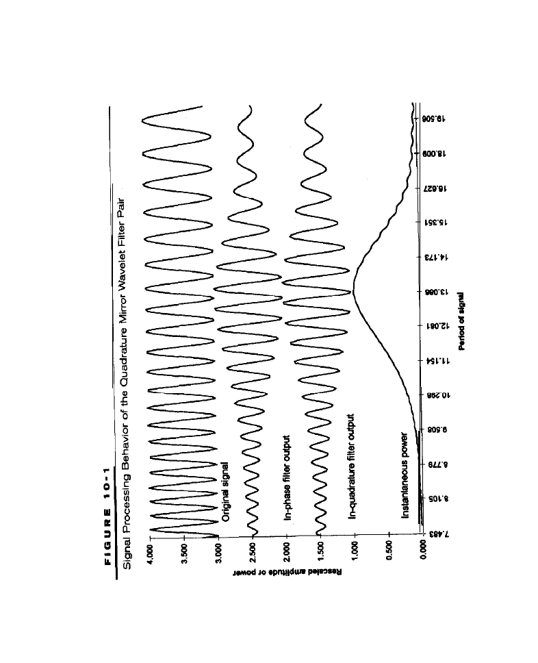
209

fourth line depicts
instantaneous
power, as estimated from the filter outputs. This
represents the strength or amplitude of cyclic activity in the signal near the center
of the
pass-band. The curve for instantaneous power is exceedingly smooth,
reaches a peak when the signal has a periodicity matching the tuning of the filter,
and declines thereafter. In the chart, the center of the pass-band appears to occur
at a period of 13, rather than 12,
period to which the filter was set. The reason
for the slight distortion is that the periodicity of the original signal was being
rapidly swept from low to high. Since the filter needs to look back several cycles,
the spectral estimate is distorted. Nevertheless, it seems apparent that trades based
on the filtered output would be highly profitable. The scaling of the y-axis is irrel-
evant; it was done in the manner presented to make the signals appear clearly, at
separate locations, on the chart.
Figure
depicts the frequency (or periodicity) and phase response of the
filter. In this case, the filter is set to have a center, or pass-band, periodicity of 20.
The relative power curve shows the strength of the output from the filter as the sig-
nal frequency is varied, but held constant in power. The filter passes the signal to
a maximum extent when it has a frequency at the center of the pass-band, and as
the frequency moves away from the center frequency of the filter, the output of the
filter smoothly and rapidly declines. There are no side lobes in the response curve,
and the output power drops to zero as the periodicity goes down or up. The filter
has absolutely no response to a steady trend or a fixed offset-a highly desirable
property for traders, since there is then no need to fuss with de-trending, or any
other preprocessing of the input signal, before applying the filter. The phase
response also shows many desirable characteristics. For the most part, the phase
response is well within
degrees within the pass-band of the filter. At the cen-
ter of the pass-band, there is no phase shift; i.e., the in-phase filter output is exact-
ly in synchronization with the input series-a trader timing his trades would
achieve perfect entries. As with the power, the phase response is smooth and
extremely well behaved. Any engineer or physicist seeing this chart should appre-
ciate the quality of these filters. When a similar chart was generated for the
Butterworth band-pass filters (used in our 1997 study), the results were much less
pleasing, especially with regard to the filter’s phase response and offset character-
istics. Severe phase shifts developed very rapidly as the periodicity of the signal
moved even slightly away from the center periodicity of the filter. In real-life
cumstances, with imprecisely timed cycles, the phase response of those filters
would likely play total havoc with any effort to achieve good trade timing.
Figure
shows the impulse response for both outputs from the
filter pair: the in-quadrature output and the in-phase output. These curves look
almost as though they were exponentially decaying sines or cosines. The decay,
however, is not quite exponential, and there are slight, though imperceptible,
adjustments in the relative amplitudes of the peaks to eliminate sensitivity to off-
set or trend.
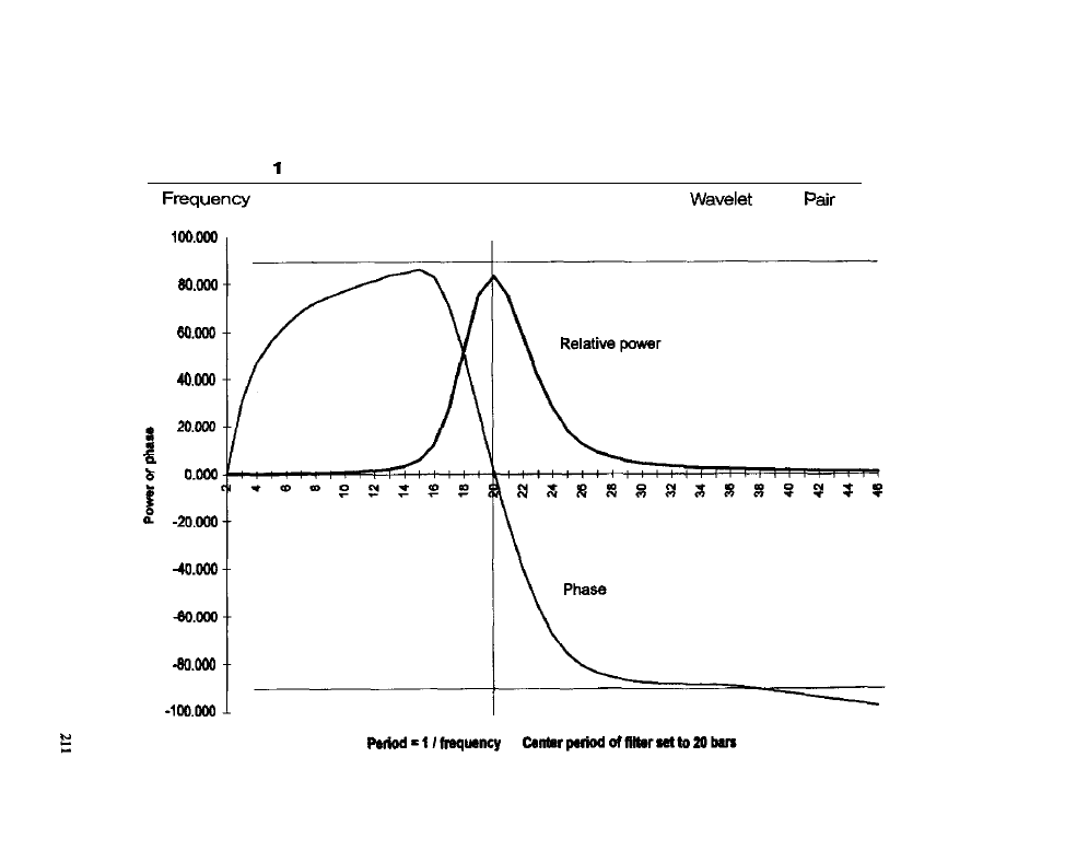
F I G U R E O - 2
(Period) and Phase Response of a Quadrature Mirror
Filter
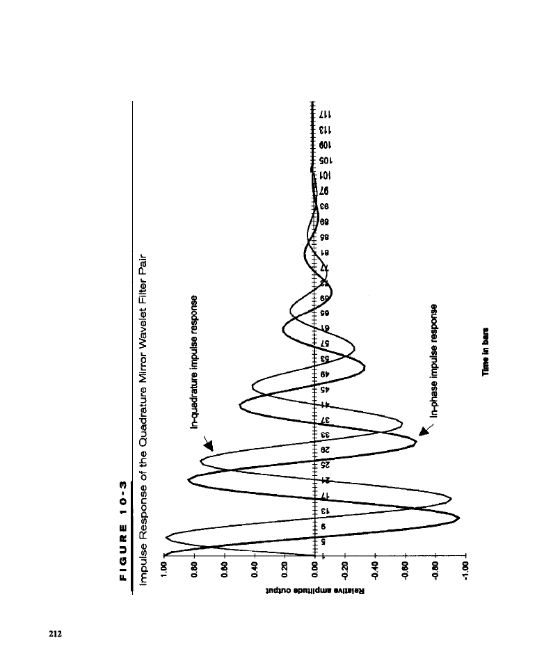

In addition to the data provided in the charts, a number of other tests were
conducted using “plasmodes.” A
is a set of data constructed to have the
characteristics that are assumed to exist in the real data. The intention is to test the
ability of some algorithm or analytic technique to properly extract, detect, or ana-
lyze those characteristics. A good cycle-based trading system should be able to do
a good job trading a synthetic data series containing lots of noise and occasional
embedded cycles. If it cannot, there could be no expectation of it trading well in
any real market. The kind of filters used in the tests below perform very well in
tests involving plasmodes.
GENERATING CYCLE ENTRIES USING FILTER
‘BANKS
One way to generate cycle entries is to set up a series of filters, each for a different
frequency or periodicity (e.g., going down a certain percentage per filter throughout
some range or spectrum that will be analyzed). If one of these filters shows strong
resonance, while the others show little or no activity, there is presumably a strong
cycle in the market. An entry is generated by looking at the pair of filter outputs and
buying at the next bar, if the cycle phase is such that a cyclic bottom will occur on
that bar, or selling at the next bar, if a cycle top is evident or would be expected on
that bar, Since the strongest-responding filter should produce no undesirable lag or
phase error, such cyclic entries should provide exceedingly timely signals if the mar-
ket is evidencing cyclic behavior. Attempting to buy cycle bottoms and sell cycle
tops is one of the traditional ways in which cycle information has been used to trade
the markets. Cycle information derived from filter banks, or by other means, can also
enhance other kinds of systems or adapt indicators to current market conditions. An
example of how information regarding the signal-to-noise ratio and periodicity of
the dominant cycle (if there is any) may be used within another system, or to adapt
an indicator to current market conditions, can be found in Ruggiero (1997).
CHARACTERISTICS OF CYCLE-BASED ENTRIES
A cycle-based entry of the kind studied below (which attempts to buy bottoms and
sell tops) has several strong characteristics: a high percentage of winning trades,
low levels of slippage, and the ability to capture as much of each move as possi-
ble. This is the kind of trading that is a trader’s dream. The assumption being made
is that there are well-behaved cycles in the market that can be detected and, more
importantly. extrapolated by this kind of technology. It has been said that the mar-
kets evidence cyclic activity up to 70% of the time. Even if clear cycles that lead
to successful trades only occur some smaller percentage of the time, because of
the nature of the model, the losses can be kept small on the failed trades by the use
of tight stops. The main disadvantage of a cycle-based entry is that the market may

have become
relative to such trading methodologies, thanks to the prolif-
eration of fairly powerful cycle analysis techniques, e.g., maximum entropy. The
trading away of well-behaved cycles may hamper all cycle detection approaches.
Since cycle entries of the kind just discussed are countertrend in nature, if the
cycles show no follow-through, but the trends do, the trader can get wiped out
unless good money management practices (tight stops) are employed. Whether or
not a sophisticated cycle analysis works, at least as implemented here, is the ques-
tion to be answered by the tests that follow.
TEST METHODOLOGY
In all tests of cycle-based entry models, the standard portfolio of 36 commodities
is used. The number of contracts in any market at any time to buy or sell on entry
was chosen to approximate the dollar volatility of two S&P 500 contracts at the
end of 1998. Exits are the standard ones in which a money management stop clos-
es
out
any trade that moves more than one volatility unit into the red, a profit tar-
get limit closes out trades that push more that four volatility units into the profit
zone, and a market-at-close order ends any trade that has not yet been closed out
by the stop-loss or profit target after 10 days has elapsed. Entry rules are specified
in the discussion of the model code and the individual tests. All tests are performed
using the standard C-Trader toolkit. Here is the code implementing the
fil-
ter entry model along with the standard exit strategy:

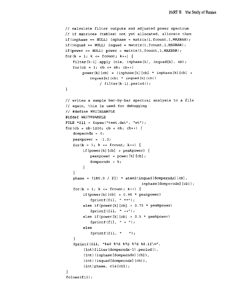
216

217


The code above implements
model being tested. The first significant
block of code specifically relevant to a cyclic trading model initializes the indi-
vidual filters that make up the filter bank. This code is set up to
only on the
pass, or when a parameter specifically affecting the computations involved in
initializing the filter bank (e.g., the width parameter) has changed; if no relevant
parameter has changed, there is no point in reinitializing the filters every time the
Model
function is called.

The next block of code applies
of the filters in the bank to the input sig-
nal. In this block, two arrays are allocated to hold the filter bank outputs. The
array contains the in-phase outputs
and the second contains the in-quad-
rature outputs
The inputs to the filters are the raw closing prices. Because
the filters
optimal, and designed eliminate offsets and trends,
there is no need to preprocess the closing prices before applying them, as might be
necessary when using less sophisticated analysis techniques. Each row in the arrays
represents the output of a single filter with a specified center frequency or
ity. Each column represents a bar.
frequencies (or periodicities) at which the fil-
ters are centered are all spaced evenly on a logarithmic scale; i.e., the ratio between
the center frequency of a given filter and the next has a fixed value. The selectivity
or bandwidth
is the only adjustable parameter in the computation of the fil-
ter banks, the correct value of which may be sought by optimization.
The usual bar-stepping loop is then entered and the actual trading signals
generated. First, a good, pure cycle to trade is identified, which involves deter-
mining the power at the periodicity that has the strongest resonance with current
market activity
The cycle periodicity at which the peak power occurs
is also assessed. If the periodicity is not at one of the end points of the range of
periodicities being examined (in this case the range is 3 bars to 30 bars), one of
the conditions for a potentially good cycle is met. A check is then made to see
what the maximum power
is at periodicities at least 2 filters away
from the periodicity at which peak power
If
is more than 1.5
times
(a signal-to-noise ratio of 1.5 or greater), the second condition
for a good cycle is met. The phase angle of that cycle is then determined (easy to
do given the pair of filter outputs), making adjustments for the slice that occurs at
180 degrees in the plane of polar coordinates. The code then checks whether the
phase is such that a cycle bottom or a cycle top is present. A small displacement
term
is incorporated in the phase assessments. It acts like the displacements
in previous models, except that here it is in terms of phase angle, rather than bars.
There is a direct translation between phase angle and number of bars; specifical-
ly, the period of the cycle is multiplied by the phase angle (in degrees), and the
sum is then divided by 360, which is the number of bars represented by the phase
angle. If the displaced phase is such that a bottom can be expected a certain num-
ber of degrees before or after the present bar, a buy is posted. If the phase angle is
such that a top can be expected, a sell signal is issued. The limit and stop prices
are then calculated, as usual. Finally, the necessary trading orders are posted.
Many other blocks of code present in the above listing have not been dis-
cussed. These were used for debugging and testing. Comments embedded in the
code should make their purpose fairly clear.
TEST RESULTS
Only one model was tested. Tests were performed for entry at the open (Test I),
entry on a limit (Test and entry on a stop (Test 3). The rules were simple: Buy
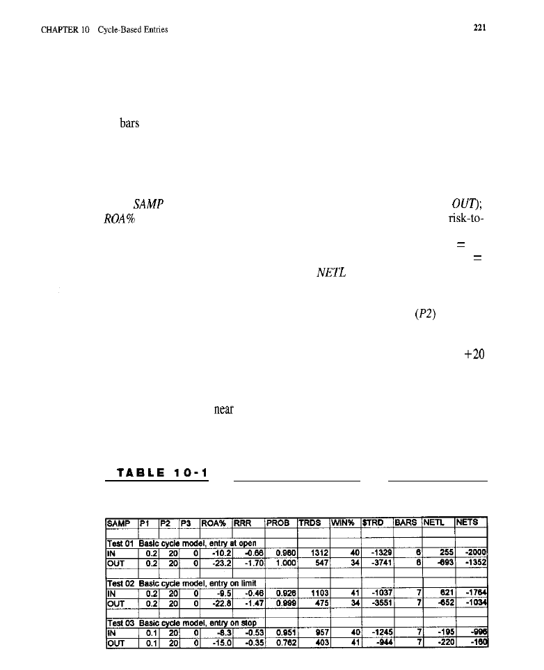
predicted cycle bottoms and sell predicted cycle tops. Exits took place when a
cycle signal reversed an existing position or when the standard strategy closed out
the trade, whichever came first. This simple trading model was first evaluated on
a noisy sine wave that was swept from a period of about 4 bars to a period of about
20
to verify behavior of the model implementation. On this data, buy and sell
signals appeared with clockwork precision at cycle tops and bottoms. The timing
of the signals indicates that when real cycles are present, the model is able to
detect and trade them with precision.
Table 10-l contains the best in-sample parameters, as well as the perfor-
mance of the portfolio on both the in-sample and verification sample data. In the
table,
= whether the test was on the optimization sample (IN or
= the annualized return-on-account; ARRR = the annualized
reward ratio; PROB = the associated probability or statistical significance; TRDS
= the number of trades taken across all commodities in the portfolio: WIN% the
percentage of winning trades; $TRD = the average profit/loss per trade; BARS
the average number of days a trade was held;
= the total net profit on long
trades, in thousands of dollars: and NETS = the total net profit on short trades, in
thousands of dollars. Two parameters were optimized. The first (PI) represents the
bandwidth for each filter in the filter bank. The second parameter
represents
the phase displacement in degrees. In all cases, the parameters were optimized on
the in-sample data by stepping the bandwidth from 0.05 to 0.2 in increments of
0.05, and by stepping the phase angle displacement from -20 degrees to
degrees in increments of 10 degrees. Only the best solutions are shown.
It is interesting that, overall, the cycle model performed rather poorly. This
model was not as bad, on a dollars-per-trade basis, as many of the other systems test-
ed, but it was nowhere
as good as the best. In-sample, the loss per trade was
$1,329 with entry at open, $1,037 with entry on limit, and $1,245 with entry on stop.
The limit order had the highest percentage of wins and the smallest average loss per
Portfolio Performance with Best In-Sample Parameters on Both In-
Sample and Out-of-Sample Data
trade. The long side was slightly profitable with entry at open, was somewhat more
profitable with entry on limit, and lost with entry on stop. The behavior out-of-sam
ple, with entry at open and on limit, was a lot worse than the behavior of the model
in-sample. The loss per trade grew to $3,741 for entry at open and to $3,551 for
entry on limit. The percentage of winning trades also declined, to 34%. The per-
formance of the cycle model on the verification sample was among the worst
observed of the various models tested. The deterioration cannot be attributed to
optimization: Several other parameter sets were examined, and regardless of
which was chosen, the cycle model still performed much worse out-of-sample.
With entry on stop, the out-of-sample performance did not deteriorate. In this case,
the loss ($944) was not too different from the in-sample loss. Although the stop
order appears to have prevented the deterioration of the model that was seen with
the other orders, in more recent times the system is a loser.
The decline of system performance in recent years was unusually severe, as
observed from the results of the other models tested. One possible reason may be
the recent proliferation of sophisticated cycle trading tools. Another explanation
might be that major trading
are conducting research using sophisticated
techniques, including
of the kind studied here. These factors may have
contributed to making the markets relatively efficient to basic cycle trading.
Table
shows the in-sample and out-of-sample behavior of the cycle
model broken down by market and entry order (test). The
column represents
the market being studied. The center and rightmost columns
contain the
number of profitable tests for a given market. The numbers in the first row repre-
sent test identifiers: 01, 02, and 03 represent entry at open, on limit, and on stop,
respectively. The last row (COUNT) contains the number of markets on which a
given model was profitable. The data in this table provides relatively detailed
information about which markets are and are not profitable when traded by each
of the models: One dash
indicates a moderate loss per trade, i.e., $2,000 to
$4,000; two dashes
represent a large loss per trade, i.e., $4,000 or more; one
plus sign
means a moderate profit per trade, i.e., $1,000 to $2,000; two plus-
es
indicate a large gain per trade, i.e., $2,000 or more; and a blank cell
means that the loss was between $0 and $1,999 or the profit was between $0 and
$1,000 per trade. (For information about the various markets and their symbols,
see Table 11-l in the “Introduction” to Part II.)
Only the IO-Year Notes and Cotton showed strong profits across all
entry orders in-sample. Out-of-sample, performance on these markets was miser-
able. The S&P 500, a market that, in our experience, has many clear and tradable
cycles, demonstrated strong profitability on the in-sample data when entry was at
open or on limit. This market was strongly profitable out-of-sample with entry on
limit and on stop, but somewhat less profitable with entry at open. Interestingly,
the
although evidencing strong in-sample profits with entry at open and on
limit, had losses out-of-sample across
three orders. There are a few other
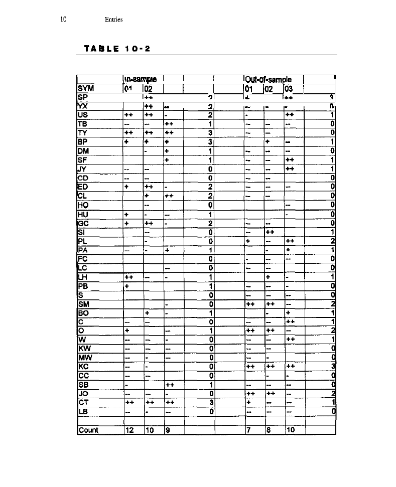
CHAPTER
Cycle-Based
223
Performance Data Broken Down by Market and Test
,
0 3
count
count
I++
I- I
I**
I
. .
I
I-
++
I

in-sample market-order combinations, as well as out-of-sample
order combinations, However, very
correspondence between the two was
observed. Perhaps markets that have not had cycles in the past (in-sample) have
cycles in the present (out-of-sample), and vice versa. At least the S&P 500
behaved as expected on the basis of prior research and may be one of the few mar-
kets consistently amenable to cycle trading in this crude form.
Figure
depicts the equity for the portfolio with entry at open. Equity
declined slowly and then became rather flat until about August 1992, at which
time it began a steady and rapid decline.
CONCLUSION
In our May 1997 study, the filter bank method appeared to have potential as the
basis for an effective trading strategy. At times it worked incredibly well, and was
almost completely insensitive to large variations in its parameters, whereas at
other times it performed poorly. The results may simply have been due to the fact
that the implementation was “quick and dirty.” Back then, the focus was on the
S&P 500, a market that continued to trade well in the present study.
The results of the current study are disappointing, all the more given the the-
oretical elegance of the filters. It may be that other approaches to the analysis of
cycles, e.g., the use of maximum entropy, might have provided better perfor-
mance; then again, maybe not. Other traders have also experienced similar disap-
pointments using a variety of techniques when trading cycles in a simple,
buy-the-bottom/sell-the-top manner. It may be that cycles are too obvious and
detectable by any of a number of methods, and may be traded away very quickly
whenever they develop in the market. This especially seems the case in recent
years with the proliferation of cycle analysis software. The suggestion is not that
cycles should be abandoned as a concept, but that a more sophisticated use of
detected cycles must be made. Perhaps better results would ensue if cycles were
combined with other kinds of entry criteria, e.g., taking trades only if a cycle top
corresponds to an expected seasonal turning-point top.
Further studies are needed to determine whether the cycle model does indeed
have the characteristic of giving precise entries when it works, but failing miser-
ably when it does not work. Looking over a chart of the S&P 500 suggests this is
the case. There are
strings of four or five trades in a row, with entries
that occur precisely at market tops and bottoms, as if predicted with perfect hind-
sight. At other times, entries occur exactly where they should not. With a system
that behaves this way, our experience indicates that, combined with a proper exit,
sometimes great profits can be achieved. More specifically, losses have to be cut
very quickly when the model fails, but trades should not be prematurely terminat-
ed when the model is correct in its predictions. Because of the precision of the
model when the predictions are correct, an extremely tight stop could perhaps
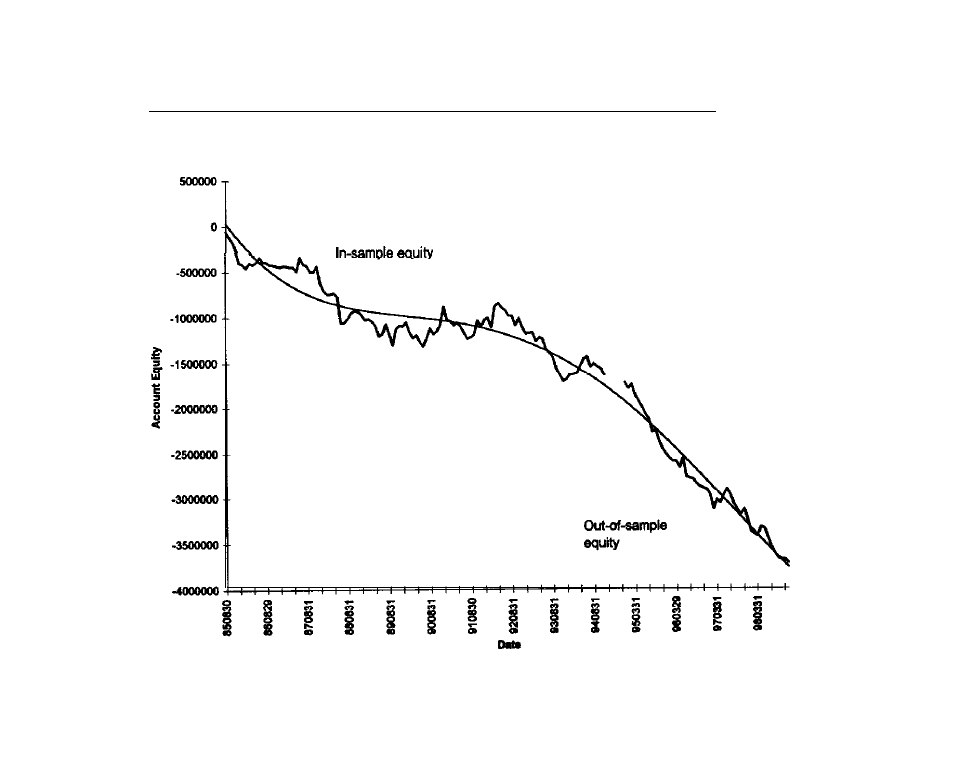
F I G U R E 1 O - 4
Portfolio Equity Growth for Count&rend Cycle Trading

226
accomplish the goal. When an exact cycle top or bottom is caught, the market
begins to move immediately in the favored direction, with hardly any adverse
excursion, and the stop is never hit. When the model fails, the stop is hit very
quickly, resulting in only a small loss. Given the fairly loose stop of the standard
exit, the benefits of sophisticated cycle trading may not have been realized.
WHAT HAVE WE LEARNED?
n
Models that are theoretically sound, elegant, and appealing do not neces-
sarily work well when trading
markets.
n
Exception to Rule 1: The S&P 500 may respond to such methods; it did
so both in our earlier study and in the current one.
. When the model does work, it does so remarkably well. As stated earlier,
when examining its behavior on the S&P 500 and several other markets,
one can quickly and easily find strings of signals that pick off tops and
bottoms with the precision of hindsight.
. The previous point suggests that exits specifically designed for a system
yields high precision when correct, but fails badly when incorrect,
may he required.
. The markets appear to have become more efficient relative to cycle
models, as they have to breakout models. Obvious market behavior
(such as clear, tradable cycles) are traded away before most traders can
capitalize on them. The lesson: Anything too theoretically appealing or
obvious will tend not to work.

Neural Networks
N
eural network technology, a form of artificial intelligence (or AI), arose from
endeavors to emulate the kind of information processing and decision making
that occurs in living organisms. The goal was to model the behavior of neural tis-
sue in living systems by using a computer to implement structures composed of
simulated neurons and neural interconnections (synapses). Research on neural
networks began in the 1940s on a theoretical level. When computer technology
became sophisticated enough to accommodate such research, the study of neural
networks and their applications began in earnest. It was not, however, until the
mid-to-late 1980s that neural network technology became of interest to the finan-
cial community. By 1989, a few vendors of neural network development tools
were available, and there was one commercial S&P 500 forecasting system based
on this technology (Scientific Consultant Services’
In the early
interest peaked, more development tools appeared, but the fervor then waned for
reasons discussed later.
While it is not within the scope of this book to present a full tutorial on neur-
al network technology, below is a brief discussion to provide basic understanding.
Those interested in exploring this subject in greater depth should read our
to
the
books
Virtual Trading
(Lederman and Klein, 1995) and
Computerized
Trading
(Jurik,
in which we also present detailed informa-
tion on system development using neural networks, as well as our articles in
Technical Analysis of Stocks and Commodities
(Katz, April 1992; Katz and
McCormick, November 1996, November 1997). Neural
Networks in Finance and
and Turban, 1993) should also be of interest.

WHAT ARE NEURAL NETWORKS?
Neural
(or “nets”) are basically building blocks that learn and are useful
for pattern recognition, classification, and prediction. They hold special appeal to
traders because nets are capable of coping both with probability estimates in
uncertain situations and with “fuzzy” patterns, i.e., those recognizable by eye but
difficult to define in software using precise rules; and they have the potential to
recognize almost any pattern that exists. Nets can also integrate large amounts of
information without becoming stifled by detail and can be made to adapt to chang-
ing markets and market conditions.
A variety of neural networks are available, differing in terms of their “archi-
tecture,” i.e., the ways in which the simulated neurons are interconnected, the
details of how these neurons behave (signal processing behavior or “transfer func-
tions”), and the process through which learning takes place. There are a number of
popular kinds of neural networks that are of some use to traders: the Kohonen and
the Learning Vector
(LVQ) networks, various adaptive resonance net-
works, and recurrent networks. In this chapter, the most popular and, in many
respects, the most useful kind of network is discussed: the “feed-forward” network.
As mentioned above, nets differ in the ways they learn. The system develop-
er plays the role of the neural network’s teacher, providing the net with examples
to learn from. Some nets employ “supervised learning” and others “unsupervised
learning.”
Supervised learning
occurs when the network is taught to produce a cor-
rect solution by being shown instances of correct solutions. This is a form of
paired-associate learning:
The network is presented with pairs of inputs and a
desired output; for every set of inputs, it is the task of the net to learn to produce
the desired output.
Unsupervised learning,
on the other hand, involves nets that
take the sets of inputs they are given and organize them as they see tit, according
to patterns they
therein. Regardless of the form of learning employed, the
main difficulty in developing successful neural network models is in finding and
“massaging” historical data into training examples or “facts” that highlight rele-
vant patterns so that the nets can learn efficiently and not be put astray or con-
fused; “preprocessing” the data is an art in itself.
The actual process of learning usually involves some mechanism for updat-
ing the neural connection weights in response to the training examples. With
forward architectures, back-propagation, a form of steepest-descent optimization,
is often used. Genetic algorithms are also effective. These are very
ally intensive and time-consuming, but generally produce better final results.
Feed-Forward Neural Networks
A
feed-forward network
consists of layers of neurons. The
input layer, the
layer, receives data or
inputs
from the outside world. The inputs consist of
inde-
pendent variables (e.g.,
market or indicator variables upon which the system is to
be based) from
some inference is to be drawn or a prediction is to be made.
The input layer is massively connected to
next layer, which is often called the
hidden
layer because it has no connections to
outside world. The outputs of the
hidden layer are fed to the next layer, which may be another hidden layer (if it is,
the process repeats), or it may be the output layer. Each neuron in the output layer
produces an output composed of the predictions, classifications, or decisions made
by the network. Networks are usually identified by the number of neurons in each
layer: For example, a 10-3-l network is one that has 10 neurons in its first or input
layer, 3 neurons in its middle layer, and 1 neuron in its output layer. Networks vary
in size, from only a few neurons to thousands, from only three layers to dozens;
the size depends on the complexity of the problem. Almost always, a three- or
four-layer network suffices.
Feed-forward networks (the kind being used in this chapter) implement a par-
ticular form of nonlinear multiple regression. The net takes a number of input vari-
ables and uses them to predict a target, exactly as in regression. In a standard linear
multiple regression, if the goal is to predict cholesterol (the dependent variable or
target) on the basis of dietary fat intake and exercise (the independent variables or
inputs), the data would be modeled as follows: predicted cholesterol = a
b
* fat
intake + * exercise: where a,
b,
and represent parameters that would be deter-
mined by a statistical procedure. In a least-squares sense, a line, plane, or
plane (depending on the number of independent variables) is being fitted to the
points in a data space. In the example above, a plane is being fit: The x-axis repre-
sents fat intake,
y-axis is exercise, and the height of the plane at each
coor-
dinate pair represents predicted cholesterol.
When using neural network technology, the two-dimensional plane or
dimensional hyperplane of linear multiple regression is replaced by a smooth
dimensional curved surface characterized by peaks and valleys, ridges and
As an example, let us say there is a given number of input variables and a goal of
finding a nonlinear mapping that will provide an output from the network that best
fits the target. In the neural network, the goal is achieved via the “neurons,” the non-
linear elements that are connected to one another. The weights of the
are
adjusted to fit the surface to the data. The learning
adjusts the weights to
get a particular curved surface that best fits the data points. As in a standard multi-
ple regression model, in which the coefficients of the regression are needed to define
the slope of the plane or hyperplane, a neural model requires that parameters, in the
form of connection weights, be determined so that the particular surface generated
(in this case a curved surface with hills and dales) will best fit the data.
NEURAL NETWORKS IN TRADING
Neural networks had their heyday in the late 1980 and early 1990s. Then the hon-
eymoon ended. What happened? Basically, disillusionment set in among traders

who believed that this new technology could, with little or no effort on the trader’s
part, magically provide the needed edge. System developers would “train” their
nets on raw or mildly preprocessed data, hoping the neural networks themselves
would discover something useful. This approach was
nothing is ever so sim-
ple, especially when trading the markets. Not only was this “neural newbie”
approach an ineffective way to use neural networks, but so many people were
attempting to use nets that whatever edge was originally gained was nullified by
the response of the markets, which was to become more efficient with regard to
the technology. The technology itself was blamed and discarded with little con-
sideration to the thought that it was being inappropriately applied. A more sophis-
ticated, reasoned approach was needed if success was going to be achieved.
Most attempts to develop neural network forecasting models, whether in a
simplistic manner or more elaborately, have focused on individual markets. A seri-
ous problem with the use of individual markets, however, is the limited number of
data points available on which to train the net. This situation leads to grand oppor-
tunities for curve-fitting (the bad kind)--something that can contribute greatly to
the likelihood of failure with a neural network, especially with less
ideal data
preprocessing and targets. In this chapter, however, neural networks will be trained
on a whole portfolio of
resulting in the availability of many tens of thou-
sands of data points (facts), and a reduction in curve-fitting for small to
sized networks. Perhaps, in this context, a fairly straightforward attempt to have a
neural network predict current or near-future market behavior might be success-
ful. In essence, such a network could be considered a universal market forecaster,
in that, trained across an entire portfolio of tradables, it might be able to predict
on all markets, in a non-market-specific fashion.
FORECASTING WITH NEURAL NETWORKS
Neural networks will be developed to predict (1) where the market is in terms of
its near-future range and (2) whether tomorrow’s open represents a turning point.
Consider,
the goal of predicting where the market is relative to its near-future
range. An attempt will be made to build a network to predict a time-reversed
Stochastic, specifically the time-reversed Slow %K. This is
usual Stochastic,
except that it is computed with time running backward. The time-reversed Slow
%K reflects where the current close lies with respect to the price range over the
next several bars. If something could predict this, it would be useful to the trader:
Knowing that today’s close, and probably tomorrow’s open, lies near the bottom of
the range of the next several days’ prices would suggest a good buy point; and
knowing
today’s close, or tomorrow’s open, lies near the top of the range
would be useful in deciding to sell. Consider, second, the goal of predicting whether
tomorrow’s open is a top, a bottom, or neither. Two neural networks will be trained.
One will predict whether tomorrow’s open represents a bottom turning point, i.e.,

has a price that is lower than the prices on earlier and later bars. The other will pre-
dict whether tomorrow’s open represents a top turning point, i.e., has a price that is
higher than the prices on earlier or later bars. Being able to predict whether a bot-
tom or a top will occur at tomorrow’s open is also useful for the trader trying to
decide when to enter the market and whether to go long or short. The goal in this
study is to achieve such predictions in any market to which the model is applied.
GENERATING ENTRIES WITH NEURAL
PREDICTIONS
Three nets will be trained, yielding three entry models.
models will be
for turning points. One model will be designed to detect bottoms, the other
model to detect tops. For the bottom detection model, if the neural net indicates that
the probability that tomorrow’s open will be a bottom is greater than some thresh-
old, then a buy order will be posted. For the top detection model, if the neural net
indicates that the probability that tomorrow’s open will be a top is greater than
some other threshold, then a sell order will be posted. Neither model will post an
order under any other
These rules amount to nothing mom
a
simple strategy of selling predicted tops and buying predicted bottoms. If, with bet-
ter than chance accuracy, the locations of bottoms and tops can be detected in time
to trade them, trading should be profitable. The detection system does not have to
be perfect, just sufficiently better than chance so as to overcome transaction costs.
For the model that predicts the time-reversed Slow
a similar strategy will
be used. If the prediction indicates that the time-reversed Slow %K is likely to be
less than some lower threshold, a buy will be posted; the market is near the bottom
of its near-future range and so a profit should quickly develop. Likewise, if the pre-
dicted reverse Slow %K is high, above an upper threshold, a sell will be posted.
These entries share the characteristics of other entries based on predictive, rather
than responsive, analysis. The entries lend themselves to countertrend trading and, if
the predictions are accurate, can dramatically limit transaction costs in
form of slip-
page, and provide good fills since the trader will be buying when others are selling and
vice versa. A good predictive model is the trader’s Holy Grail, providing the ability to
sell near tops and buy near bottoms. As with other predictive-based entries, if the pre-
dictions are not sufficiently accurate, the benefits will be outweighed by the costs of
bad trades when the predictions go wrong,
they often do.
TIME-REVERSED SLOW %K MODEL
The first step in developing a neural forecasting model is to prepare a
set, which is the sample of data consisting of examples from which the net learns;
i.e., it is the data used to train the network and to estimate certain statistics. In this
case, the fact set is generated using the in-sample data from all commodities in the

portfolio. The number of facts in the
set is, therefore, large-88,092 data
points. A fact set is only generated for training, not for testing, for reasons that will
be explained later.
To generate the facts that make up the fact set for this model, the initial step
of computing the time-reversed Slow
which is to serve as the target,
must
be
taken. Each fact is then created and written to a file by stepping through the
sample bars for each commodity in the portfolio. For each current bar (the one cur-
rently being stepped through), the process of creating a fact begins with computing
each input variable in the fact. This is done by calculating a difference between a
pair of prices, and then dividing that difference by the square-root of the number
of bars that separate the two prices. The square-root correction is used because, in
a random market, the standard deviation of a price difference between a pair of
bars is roughly proportional to the square-root of the number of bars separating the
two prices. The correction will force each price difference to contribute about
equally to the fact. In this experiment, each fact contains 18 price changes that are
computed using the square-root correction. These 18 prices change scores will
serve as the 18 inputs to the neural network after some additional processing.
The pairs of prices (used when computing the changes) are sampled with
increasing distance between them: i.e., the further back in time, the greater the dis-
tance between the pairs. For the first few bars prior to the current bar, the spacing
between the prices
is only 1 bar; i.e., the price of the bar prior to the
current bar is be subtracted from the price of the current bar; the price 2 bars
before the current bar is subtracted from the price bar ago, etc. After several such
price change scores, the sampling is increased to every 2 bars, then every 4, then
every 8, etc. The exact spacings are in a table inside the code. The
rationale
behind
this procedure is to obtain
detailed information on very recent price behav-
ior. The further back the prices are in time, the more likely only longer-term move-
ments will be significant. Therefore, less resolution should be required. Sampling
the bars in this way ought to provide
resolution to detect cycles and other
phenomena that range from a period of 1 or 2 bars through 50 bars or more. This
approach is in
accord
with a suggestion made by Mark
After assembling the
input variables consisting of the square-root-cor-
rected price differences for a fact, a normalization procedure is applied. The inten-
tion is to preserve wave shape while discarding amplitude information, By treating
the 18 input variables as a vector, the normalization consists of scaling the vector
to unit length. The calculations involve squaring each vector element or price dif-
ference, summing the squares, taking the square-root, and then dividing each ele-
ment by the resultant number. These are the input variables for the neural network.
In actual fact, the neural network software will further scale these inputs to an
appropriate range for the input neurons.
The target (dependent variable in regression terms) for each fact is simply the
time-reversed Slow %K for the current bar. The input variables and target for each

fact are written in simple ASCII format to a file that can be analyzed with a good
neural network development package.
The resultant fact set is used to train a net to predict the time-reversed Slow
%K, i.e., to predict the relative position of today’s close, and, it is hoped, tomor-
row’s open, with respect to the range of prices over the next 10 bars (a
reversed Slow
The next step in developing the neural forecaster is to actually train some
neural networks using the just-computed fact set. A series of neural networks,
varying in size, are trained. The method used to select the most appropriately sized
and trained network is not the usual one of examining behavior on a test set con-
sisting of out-of-sample data. Instead, the correlation coefficients, which reflect
the predictive capabilities of each of the networks, are corrected for shrinkage
based on the sample size and the number of parameters or connection weights
being estimated in the corresponding network. The equation employed to correct
for shrinkage is the same one used to correct the multiple correlations derived
from a
regression (see the chapters on optimization and statistics).
Shrinkage is greater for larger networks, and reflects curve-fitting of the undesir-
able kind. For a larger network to be selected over a smaller network, i.e., to over-
come its greater shrinkage, the correlation it produces must be sufficiently greater
than that produced by the smaller network. This technique enables networks to be
selected without the usual reference to out-of-sample data. All networks are fully
trained: i.e., no attempt is being made to compensate for loss of degrees of free-
dom by undertraining.
The best networks, selected on the basis of the shrinkage-corrected correla-
tions, are then tested using the actual entry model, together with the standard exit,
on both in- and out-of-sample data and across all markets. Because shrinkage results
from curve-fitting, excessively curve-fit networks should have very poor
corrected correlations. The large number of facts in the fact set (88,092) should help
reduce the extent of undesirable curve-fitting for moderately sized networks.
Code for the Reverse Slow %K Model
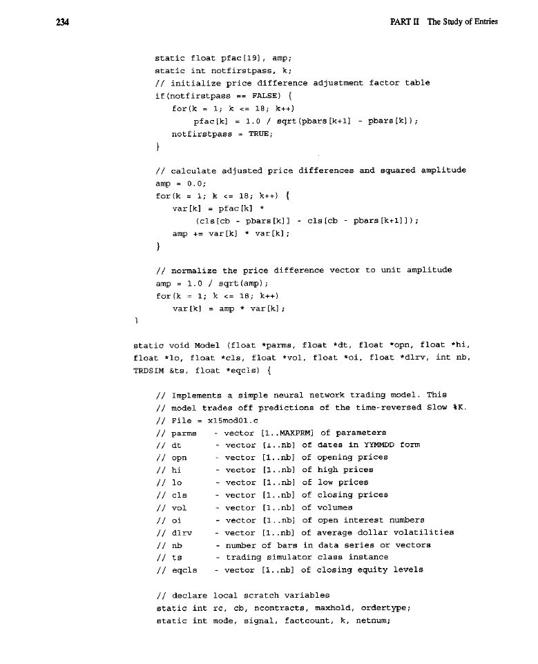
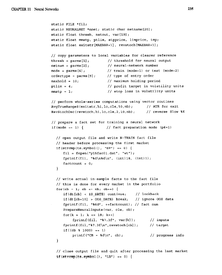


The code is comprised of two functions: the usual function that implements the
trading model (Model), and a procedure to prepare the neural network inputs
The procedure that prepares the inputs requires the index
of the current bar
(cb)
and a series of closing prices
on which to operate.
The
function, given the index to the currant bar and a
series of closing prices, calculates all inputs for a given fact that are required for the
neural network. In
list,
the
numbers after the
zero (which is ignored),
are the lookbacks, relative to the current bar, which are used to calculate the price
differences discussed earlier. The first block of code, after the declarations, initial-
izes a price adjustment factor table. The table
on the first pass through
the function and contains the square-roots of the number of bars between each pair
of prices from which a difference is computed. The next block of code calculates the
adjusted price differences, as well as the sum of the squares of these differences, i.e.,

the squared amplitude or length of the resultant vector. The final block of code in
this
function
normalizes the vector of price differences to unit length.
The general code
implements the model follows our standard practice.
After a block of declarations, a number of parameters are copied to local variables for
convenient reference. The
average true range, which is used for the standard
exit, and the time-reversed
Slow %K, used as a target, are then computed.
One of the parameters (mode) sets the mode in which
code will
A
mode of 1 runs the code to prepare a fact file: The file is opened, the header (con-
sisting of the number of inputs, 18, and the number of targets, 1) is written, and the
fact count is initialized to zero. This process only occurs for the first market in the
portfolio. The tile remains open during further processing until it is closed after
the last tradable in the portfolio has been processed. After the header, facts are writ-
ten to the tile. All data before
in-sample date and after the out-of-sample date
are ignored. Only the in-sample data are used. Each fact written to the file consists
of a fact number, the 18 input variables (obtained using
and
the target (which is the time-reversed Slow %K). Progress
is displayed
for the user as the fact file is prepared.
If
mode
is set to 2, a neural network that has been trained using the fact tile
discussed above is used to generate entries into trades, The first block of code
opens and loads the desired neural network before beginning to process the first
commodity. Then
standard loop begins. It steps through bars to simulate actu-
al trading. After executing
usual code to update the simulator, calculate the
number of contracts to trade, avoid limit-locked days, etc.,
block of code is
reached that generates the entry signals, stop prices, and limit prices. The
function is called to generate
inputs corresponding to the
current bar, these inputs are fed to the net, the network is told to run itself, the out-
put
the net is retrieved, and the entry signal is generated.
The rules used to generate
entry signal are as follows. If the output from the
network is greater than a threshold (thresh), a sell signal is issued; the net is predicting
a high
for the
time-reversed Slow
%K, meaning that the current closing price
might be near the high of its near-future range. If
output from the network (the pre-
diction of the time-reversed Slow %K) is below 100 minus thresh, a buy signal is
issued. As
example, if
thresh
were set to 80, any
Slow %K
greater than 80 would result in the posting of a sell signal, and any predicted time-
reversed Slow %K less than 20 would result in the issuing of a buy signal.
Finally, there are the two blocks of code used to issue the actual entry orders
and to implement the standardized exits. These blocks of code are identical to
those
have appeared and been discussed in previous chapters.
Test Methodology for the Reverse Slow %K Model
The model
is
executed with the
mode
parameter set to
1
to generate a fact set. The
fact set is loaded into N-TRAIN, a neural network development kit (Scientific

Consultant Services,
appropriately scaled for neural processing,
and shuffled, as required when developing a neural network. A series of networks
are then trained, beginning with a small network and working up to a fairly large
network. Most of the networks are simple,
nets. Two
networks are
also trained. All nets are trained to maximum convergence and then “polished” to
remove any small biases or offsets. The process of polishing is achieved by reduc-
ing the learning rate to a very small number and then continuing to train the net for
about
runs.
Table 1 l-l contains information regarding all networks that were trained for
this model, along with the associated correlations and other statistics. In the table,
= the file name to which the net was saved; Net
Size
= the number of
layers and the number of neurons in each layer;
= the number of con-
nections in the net optimized by the training process (similar to the number of
regression
in a multiple regression in terms of their impact on
fitting and shrinkage); and
= the multiple correlation of the network
output with the target (this is not a squared multiple correlation but an actual cor-
relation). Corrected for Shrinkage covers two columns: The left one represents the
correlation corrected for shrinkage under the assumption of an effective sample
size of 40,000 data points or facts in the training set. The right column represents
the correlation corrected for shrinkage under the assumption of 13,000 data points
or facts in the training set. The last line of the table contains the number of facts
or data points
(Actual
and the number of data points assumed for each of the
shrinkage corrections
(Assumed).
The number of data points specified to the shrinkage adjustment equation is
smaller than the actual number of facts or data points in the training set. The reason
Training Statistics for Neural Nets to Predict Time-Reversed Slow
18-8-l
152
18-12-l
2 2 8
312

is the presence of redundancy between facts. Specifically, a fact derived from one
bar is likely to be fairly similar to a fact derived from an immediately adjacent bar.
Because of the similarity,
“effective” number of data points, in terms of con-
tributing statistically independent information, will be smaller than the actual num-
ber of data points. The two corrected correlation columns represent adjustments
assuming two differently reduced numbers of facts. The process of correcting corre-
lations is
analogous
to that of correcting probabilities for multiple tests in optimiza-
tion: As a parameter is stepped through a number of values, results are likely to be
similar for nearby parameter values, meaning the effective number of tests is
what less
the actual number of tests.
Training Results for Time-Reversed Slow %K Model
As evident from Table 1 l-l, the raw correlations rose monotonically with the size
of the network
in
terms of numbers of connections. When adjusted for shrinkage,
by assuming an effective sample size of 13,000,
picture changed dramatically:
The nets that stood out were the small
net with 6 middle layer neurons, and
the smaller of the two 4-layer networks. With the more moderate shrinkage cor-
rection, the two large 4-layer networks had the highest estimated predictive abili-
ty, as indicated by the multiple correlation of
outputs
the target.
On the basis of
more conservative statistics (those assuming a smaller
effective sample size and, hence, more shrinkage due to curve-fitting) in Table 1
1, two neural nets were selected for
use
in the entry model: the 18-6-l network
and the 18-14-4-l network
These were considered the best
bets for nets that might hold up out-of-sample. For the test of the entry model
using
these nets, the model implementation was run
mode set to 2. As usual,
all order types (at open, on limit, on stop) were tested.
TURNING-POINT MODELS
For these models, two additional fact sets are needed. Except for their targets,
fact sets are identical to the one constructed for the time-reversed Slow
The target for the first fact set is a 1, indicating a bottom turning point, if tomor-
row’s open is lower than the 3 preceding bars and
10
succeeding bars. If not, this
target is set to 0. The target for the second fact set is a indicating a top, if tomor-
row’s open has a price higher than the preceding 3 and succeeding
opens.
Otherwise this target is set to 0. Assuming there are consistent patterns in the
ket, the networks should be able to learn them and, therefore, predict whether
tomorrow’s open is going to be a top, a bottom, or neither.
Unlike the fact set for the time-reversed Slow %K
model, the
facts in the sets
for these models are generated only if tomorrow’s open could possibly be a turn
ing point. If, for example, tomorrow’s open is higher than today’s open,

tomorrow’s open cannot be considered a turning point, as defined earlier, no mat-
ter what happens thereafter. Why ask the network to make a prediction when there
is no uncertainty or need? Only in cases where there is an uncertainty about
whether tomorrow’s open is going to be a turning point is it worth asking the net-
work to make a forecast. Therefore, facts are only generated for such cases.
The processing of the inputs, the use of statistics, and all other aspects of the
test methodology for the turning-point models are identical to that for the
reversed Slow %K model. Essentially, both models are identical, and so is the
methodology; only the subjects of the predictions, and, consequently, the targets
on which the nets are trained, differ. Lastly, since the predictions are different, the
rules for generating entries based on the predictions are different between models.
The outputs of the trained networks represent the probabilities, ranging from
0 to of whether a bottom, a top, or neither is present. The two sets of rules for
the two models for generating entries are as follows: For the
model, if the bot-
tom predictor output is greater than a threshold, buy. For the second model, if the
top predictor output is greater than a threshold, sell. For both models, the thresh-
old represents a level of confidence that the nets must have that there will be a bot-
tom or a top before an entry order is placed.
write
actual in-sample facts to the fact
file
= 1;
(
if
continue;
if
ignore
data
3 ,
continue;
number
inputs
Lowest
1.0;
= 0.0;
target
t a r g e t
=
,
progress
info
generate entry
signals.
stop prices and
limit
prices
3 ,
r u n
preprocess
net inputs
net
=
get
100.0;
percent

Since the code for the bottom predictor model is almost identical to that of the time-
reversed Slow %K model, only the two blocks that contain changed code are pre-
sented above. In the first block of code, the time-reversed Slow %K is not used.
Instead, a series of ones or zeros is calculated that indicates the presence (1) or
absence
of bottoms (bottom target). When writing the facts, instead of
the
time-reversed Slow %K, the bottom target is written. In the second block of code, the
roles for comparing the neural output with an appropriate threshold, and generating
the actual entry buy signals, are implemented. In both blocks, code is included to pre-
vent the writing of facts, or use of predictions, when tomorrow’s
could not pos-
sibly be a bottom. Similar code fragments for the top predictor model appear below.
ignore
data
skip these facts
number
target
write target

Test Methodology for the Turning-Point Model
The test methodology for this model is identical to that used for the time-reversed
Slow %K model. The fact set is generated, loaded into N-TRAIN, scaled, and shuf-
fled. A series of nets (from
to 4-layer ones) are trained to maximum convergence
and then polished. Statistics such as shrinkage-corrected correlations are calculated.
Training Results for the Turning-Point Model
Forecaster.
The structure of Table 1 l-2 is identical to that of Table 11-l. As
with the net trained to predict the time-reversed Slow
there was a monotonic
relationship between the number of connections in the network and the multiple cor-
relation of the network’s output with the target; i.e., larger nets evinced higher corre-
lations. The net was
on a total of 23,900 facts, which is a smaller fact set than
that for the time-reversed Slow %K. The difference in number of facts resulted
because the only facts
used were those that
contained some uncertainty
about
whether
tomorrow’s open could be a
point. Since the facts for the bottom forecaster
came from more widely spaced
in the time series, it was assumed that there
would be less redundancy among them. When corrected for shrinkage, effective sam-
ple sizes of 23,919 (equal to the actual number of facts) and 8,000 (a reduced
fact count) were assumed. In terms of the more severely adjusted correlations, the
best net in this model appeared to be the largest 4-layer network; the smaller
network was also very good. Other than these two nets, only the
network with
10 middle-layer neurons was a possible choice. For tests of trading performance, the
large
network
and the much smaller 3-layer network
were
selected.
T A B L E
Training Statistics for Neural Nets to Predict Bottom Turning Points
Net Name
Size
I
NNI
1 8 4 1
76
0.050
114
0.121
0.100
0.025
NET
1
1 5 2
‘
T
I
.
1
2-1
228
0.167
0.137
-0.019
1818-l
304
0.185
0.148
-0.080
0.188
18-200-l
488
0.200
23900
Assumed
23900
8000
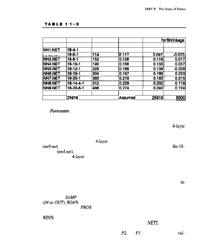
244
Training Statistics
for Neural Nets to Predict Top Turning Points
Net Name
Net Size
Connections Correlation Corrected
70
0.103
0.068
0.035
NN2 NET
Actual N
I
Top
Table 1 l-3 contains the statistics for the nets in this model; they
were trained on 25,919 facts. Again, the correlations were directly related in size to
the number of connections in the net, with a larger number of connections leading
to a better model fit. When mildly corrected for shrinkage, only the smaller
network deviated from this relationship
by
having a higher correlation than would
be expected. When adjusted under the assumption of large amounts of curve-fitting
and shrinkage, only the two
networks stood out, with the largest one
performing best. The only other high correlation obtained was for
10-l net
To maximize the difference between the nets used in the trading
tests, the largest
net, which was the best shrinkage-corrected performer, and
the fairly small (18-10-l) net were chosen.
TRADING RESULTS FOR ALL MODELS
Table 11-4 provides data regarding whole portfolio performance with the best
sample parameters for each test in the optimization and verification samples. The
information is presented for each combination of order type, network, and model.
In the table,
= whether the test was on the training or verification sample
= the annualized return-on-account;
ARRR
= the annualized
risk-to-reward ratio;
= the associated probability or statistical significance;
TRDS
= the number of trades taken across all commodities in the portfolio;
=
the percentage of winning trades;
$TRD =
the average profit/loss per
trade;
BARS
= the average number of days a trade was held;
= the
total net
profit on long trades, in thousands of dollars;
NETS = the
total net profit on short
trades, in thousands of dollars. Columns
PI,
and
represent parameter
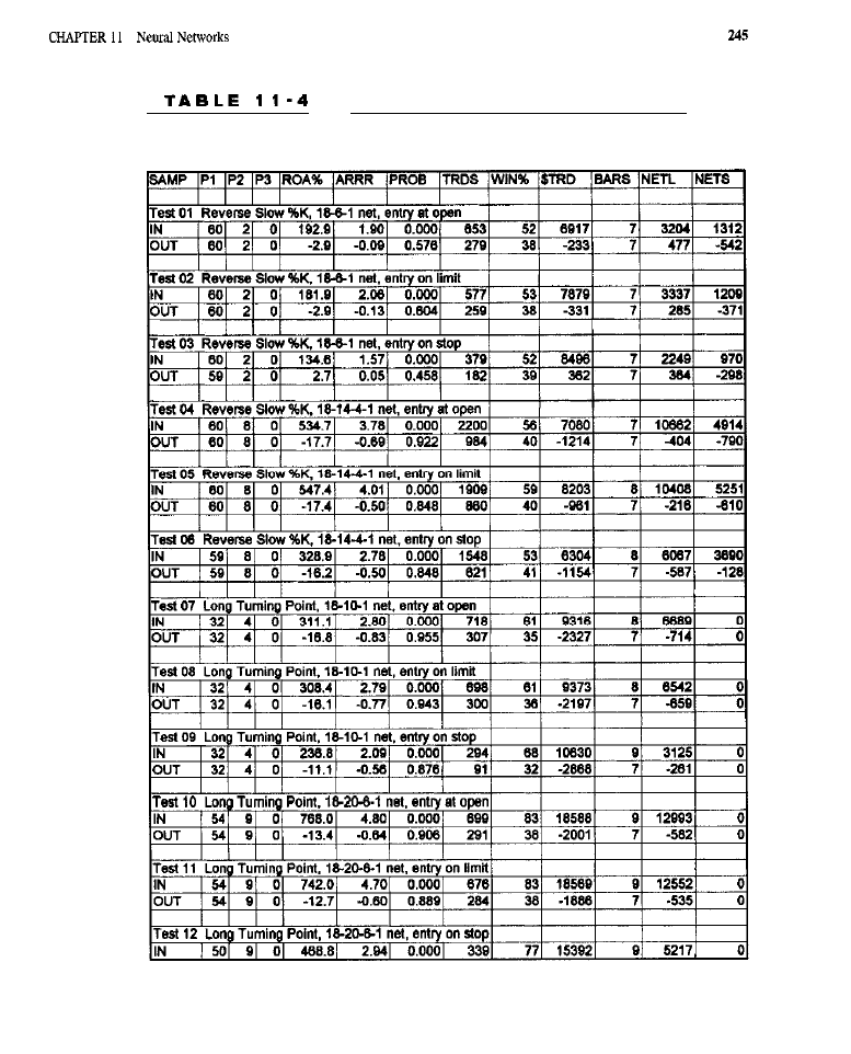
Portfolio Performance with Best In-Sample Parameters for Each Test
in the Optimization and Verification Samples
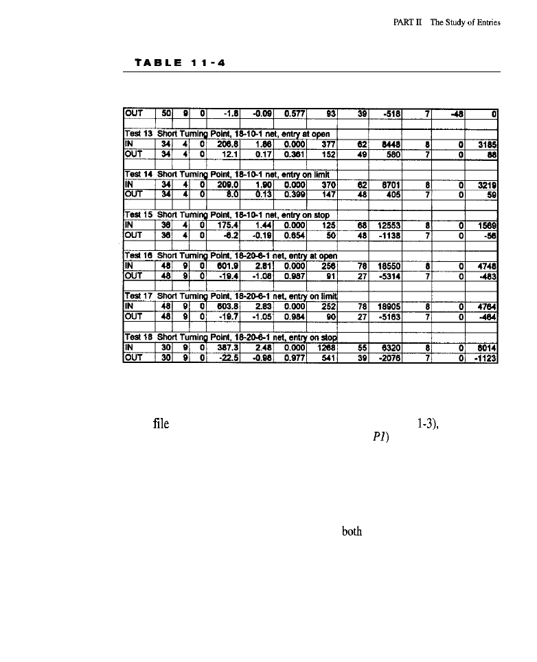
2 4 6
Portfolio Performance with Best In-Sample Parameters for Each Test
in the Optimization and Verification Samples (Continued)
ues:
PI
= the threshold,
P2 = the
number of the neural network within the group
of networks trained for the model (these numbers correspond to the numbers used
in the
names for the networks shown in Tables 1 l-l through 1
P3 =
not
used.
In all cases, the threshold parameters (column
shown are those that
resulted in the best in-sample performance. Identical parameters are used for ver-
ification on the out-of-sample data.
The threshold for the time-reversed Slow %K model was optimized for each
order type by stepping it from 50 to 90 in increments of 1. For the top and bottom
predictor models, the thresholds were stepped from 20 to 80 in increments of 2. In
each case, optimization was carried out only using the in-sample data. The best
parameters were then used to test the model on
the in-sample and out-of-sam-
ple data sets. This follows the usual practice established in this book.
Trading Results for the Reverse Slow %K Model
The two networks that were selected as most likely to hold up out-of-sample, based
on their shrinkage-adjusted multiple correlations with the target, were analyzed for

trading performance, The first network was the smaller of the two, having 3 layers
(18-6-l network). The second network had 4 layers (18-14-4-l network).
Results
Using
18-6-I Network.
In-sample, as expected, the trading results
were superb. The average trade yielded a profit of greater than $6,000 across all
order types, and the system provided an exceptional annual return, ranging from
192.9% (entry at open, Test 1) to 134.6% (entry on stop, Test 3). Results this
good were obtained because a complex model containing 114 free parameters
was
to the data. Is there anything here beyond curve-fitting? Indeed there
is. With the stop order, out-of-sample performance was actually slightly prof-
itable-nothing very tradable, but at least not in negative territory: The average
trade pulled $362 from the market. Even though losses resulted out-of-sample
for the other two order types, the losses were rather small when compared with
those obtained from many of the tests in other chapters: With entry at open, the
system lost only $233 per trade. With entry on limit (Test
it lost $331. Again,
as has sometimes happened in other tests of countertrend models, a stop order,
rather than a limit order, performed best. The system was profitable out-of-sam-
ple across all orders when only the long trades were considered. It lost across all
orders on the short side.
In-sample performance was fabulous in almost every market in the portfolio,
with few exceptions, This was true across all order types. The weakest perfor-
mance was observed for Eurodollars, probably a result of the large number of con-
tracts (hence high transaction costs) that must be traded in this market. Weak
performance was also noted for Silver, Soybean Oil, T-Bonds, T-Bills, Canadian
Dollar, British Pound, Gold, and Cocoa. There must be something about these
markets that makes them difficult to trade, because, in-sample, most markets per-
form well. Many of these markets also performed poorly with other models.
Out-of-sample, good trading was obtained across all three orders for the
Bonds (which did not trade well in-sample), the
the Swiss Franc, the
Japanese Yen, Unleaded Gasoline, Gold (another market that did not trade well
sample), Palladium, and Coffee. Many other markets were profitable for two of the
three order types. The number of markets that could be traded profitably out-of-sam-
ple using neural networks is a bit surprising. When the stop order (overall, the
performing order) was considered, even the S&P 500 and NYFE yielded substantial
profits, as did Feeder Cattle, Live Cattle, Soybeans, Soybean Meal, and Oats.
Figure 1 l-l illustrates the equity growth for the time-reversed Slow %K pre-
dictor model with entry on a stop. The equity curve was steadily up in-sample, and
continued its upward movement throughout about half of the out-of-sample peri-
od, after which there was a mild decline.
Results of the 18-14-4-l Network.
This network provided trading performance
that showed more improvement in-sample than out-of-sample. In-sample, returns
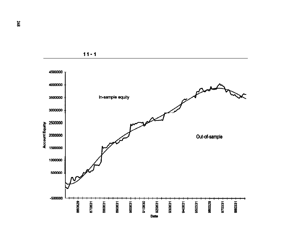
F I G U R E
Equity Growth for Reverse Slow %K 18-6-l Net, with Entry on a Stop
0
equity

ranged from a low of 328.9% annualized (stop order, Test 6) to 534.7% (entry at
open, Test 4). In all cases, there was greater than $6,000 profit per trade. As usual,
the longs were more profitable than the shorts. Out-of-sample, every order type
produced losses. However, as noted in the previous set of tests, the losses were
smaller than typical of losing systems observed in many of
other chapters: i.e.,
the losses were about $1,000 per trade, rather than $2,000. This network also took
many more trades than
previous one. The limit order performed best (Test 5).
The long side evidenced smaller losses than the short side, except in the case of
the stop order, where the short side had relatively small losses. The better in-sam-
ple performance and worsened out-of-sample performance are clear evidence of
curve-fitting. The larger network, with its 320 parameters, was able to capitalize
on the idiosyncrasies of the training data, thereby increasing its performance
sample and decreasing it out-of-sample.
In-sample, virtually every market was profitable across every order. There
were only
exceptions: Silver, the Canadian Dollar, and Cocoa. These mar-
kets seem hard to trade using any system. Out-of-sample, several markets were
profitable across all three order types: the Deutschemark, the Canadian Dollar,
Light Crude, Heating Oil, Palladium, Feeder Cattle, Live
Cattle, and
Lumber. A
few other markets traded well with at least one of the order types.
The equity curve showed perfectly increasing equity until the out-of-sample
period, at which point it mildly declined. This is typical of a curve resulting from
overoptimization. Given a sample size of 88,092 facts, this network may have
been too large.
Trading Results for the Bottom Turning-Point Model
The two networks that were selected, on the basis of their corrected multiple correla-
tions with the target, as most likely to hold up out-of-sample are analyzed for trading
performance below. The
network was the smaller of the two, having 3 layers
network). The second
was a network with 4 layers (18-20-6-I network).
Results of the 18-10-I
In-sample, this network performed exception-
ally well-nothing unusual, given the degree of curve-fitting involved.
sample, there was a return to the scenario of a heavily losing system. For all three
order types (at open, on limit, and on stop, or Tests 7, 8, and 9, respectively), the
average loss per trade was in the $2,000 range, typical of many of the losing mod-
els tested in previous chapters. The heavy per-trade losses occurred although
model was only trading long positions, which have characteristically performed
better than shorts.
In-sample, only four markets did not perform well: the British Pound, Silver,
Live Cattle, and Corn. Silver was a market that also gave all the previously tested
networks problems. Out-of-sample, the network was profitable across all three

order types for the S&P 500, the Japanese Yen, Light Crude, Unleaded Gasoline,
Palladium, Soybeans, and Bean Oil. A number of other markets were also prof-
itable with one or two of the orders.
The equity curve showed strong steady gains in-sample and losses
sample.
Results
18-20-6-I
These results were derived from Tests
(at open, on limit, and on stop, respectively). In-sample performance for this net-
work soared to unimaginable levels. With entry at open, the return was 768%
annualized, with 83% of the 699 trades taken being profitable. The average trade
produced $18,588 profit. Surprisingly, despite the larger size of this network
(therefore, the greater opportunity for curve-fitting), the out-of-sample perfor-
mance, on a dollars-per-trade basis, was better than the smaller network, especial-
ly in the case of the stop entry, where the loss per trade was down to $518.
All markets were profitable across all orders in-sample, without exception.
Out-of-sample, the S&P 500, the British Pound, Platinum, Palladium, Soybean
Meal, Wheat, Kansas Wheat, Minnesota Wheat, and Lumber were profitable
across all three order types.
Trading Results for the Top Turning-Point Model
The two networks that were selected as most likely to hold up out-of-sample,
based on their corrected multiple correlations with the target, are analyzed for
trading performance below. The first network was the smaller of the two, having
3 layers (18-10-l network). The second network had 4 layers (18-20-6-l network).
Results
of
the 18-10-I Network.
As usual, the in-sample performance was
excellent. Out-of-sample performance was profitable for two of the orders: entry
at open (Test 13) and on limit (Test 14). There were moderate losses for the stop
order (Test 15). This is slightly surprising, given that the short side is usually less
profitable than the long side.
The market-by-market breakdown reveals that only the Canadian Dollar,
Feeder Cattle, Bean Oil, Wheat, and Cocoa were not profitable across all three
order types, in-sample. Out-of-sample, strong profits were observed across all
three orders for the Deutschemark, the Japanese Yen, Light Crude, Heating Oil,
Feeder Cattle, Live Cattle, and Corn. The Japanese Yen, Light Crude, and, to some
extent, Corn shared profitability with the corresponding bottom (long)
point model; in other words, these markets held up out-of-sample for both the bot-
tom network and the top (short) network.
The equity curve (Figure 1 l-2) for entry at open depicts rapidly rising equi-
ty until August 1993, and then more slowly rising equity throughout the remain-
der of the in-sample period and through
about
two-thirds of the out-of-sample
period. Equity then declined slightly.
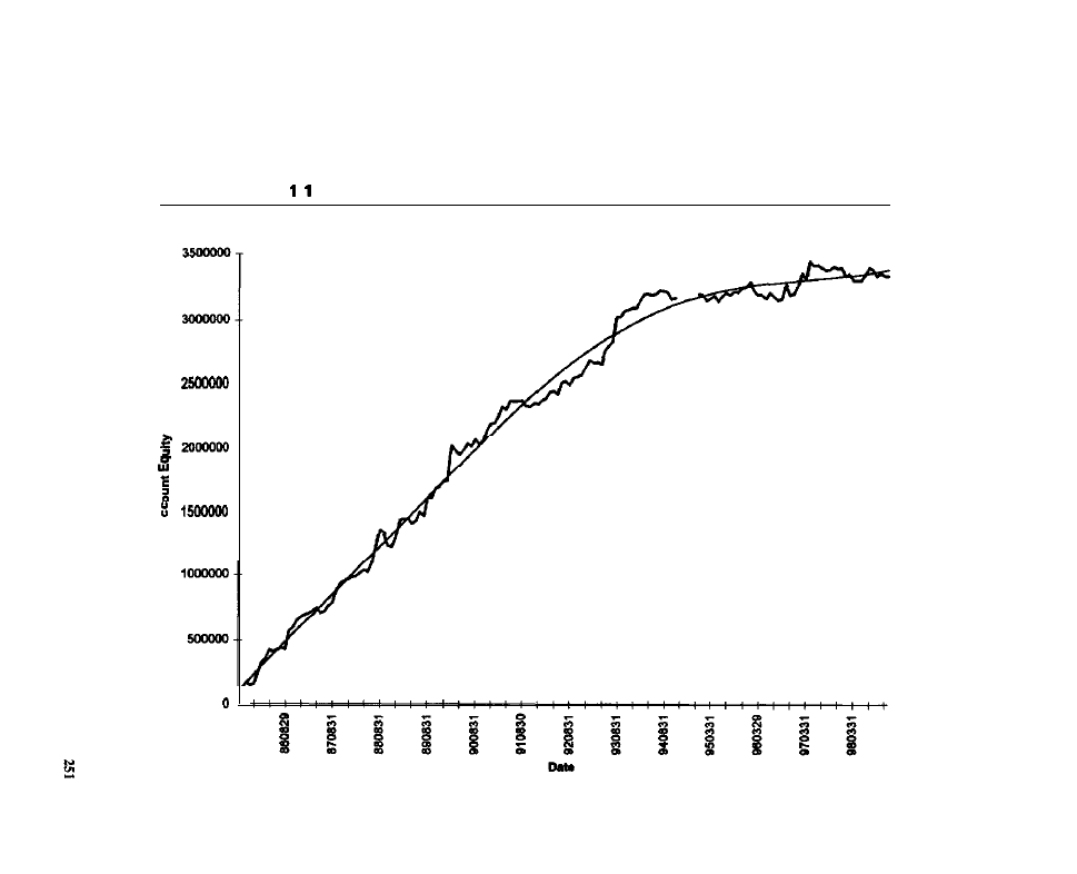
F I G U R E - 2
Equity Growth for Short Turning Points, 18-l O-l Net, with Entry at Open
4
In-sample equity
Out-of-sample equity

Results of the 18-20-6-I Network. As expected, this network, the larger of the
two, produced greater and more consistent in-sample profits due to a higher
amount of curve-fitting. Out-of-sample, this network performed terribly across all
order types (at open, on limit, and on stop, or Tests 16, 17, and 18, respectively).
The least bad results were obtained with the stop order.
In-sample, only Silver, Wheat, Sugar, and Orange Juice did not trade prof-
itably across all orders. Out-of-sample, only Cocoa showed profitability for all
three orders. Surprisingly, all the metals showed strong out-of-sample profitability
for the entry at open and on limit, as did Feeder Cattle, Cocoa, and Cotton.
Portfolio equity showed incredibly smooth and steep gains in-sample, with
losses out-of-sample for all order types.
SUMMARY ANALYSES
Table 11-5 provides in-sample and Table 11-6 contains out-of-sample perfor-
mance statistics for all of the neural network models broken down by test and mar-
ket. The
column represents the market being studied. The rightmost column
contains the number of profitable tests for a given market. The numbers
in the
row represent test identifiers. The last row
contains the num-
ber of markets on which a given model was profitable. The data in this table pro-
vides relatively detailed information about which markets are and are not
profitable when traded by each of the models: One dash (-) indicates a moderate
loss per trade, i.e., $2,000 to $4,000; two dashes
represent a large loss per
trade, i.e., $4,000 or more; one plus sign (+) means a moderate profit per trade,
i.e., $1,000 to $2,000; two pluses
indicate a large gain per trade, i.e., $2,000
or more; and a blank cell means that the loss was between $0 and $1,999 or the
profit was between $0 and $1,000 per trade. (For information about the various
markets and their symbols, see Table II-1 in the “Introduction” to Part IL)
In-sample, every order and every model yielded exceptionally strong positive
returns (see Table 1 l-7). When averaged over all models, the entry at open and on
limit performed best, while the entry on stop was the worst; however, the differ-
ences are all very small. In-sample, the best dollars-per-trade performance was
observed with the large turning-point networks for the long (bottom) and short
(top) sides. Out-of-sample, the stop order provided the best overall results. The
time-reversed Slow %K and the short (top) turning-point models performed best
when averaged across all order types.
CONCLUSION
When a neural newbie model was tested on an individual market (Katz and
McCormick, November
the conclusion was that such an approach does not
work at all. The out-of-sample behavior in some of the current tests was much

In-Sample Results Broken Down by Test and Market
ter than expected, based on our earlier explorations of simple neural network mod-
els. In the current tests, the more encouraging results were almost certainly due to
the large number of data points in the training set, which resulted from training the
model across an entire portfolio, rather than on a single tradable. In general, the
larger the optimization (or training) sample, the greater the likelihood of contin-
ued performance in the verification sample. Sample size could be increased by
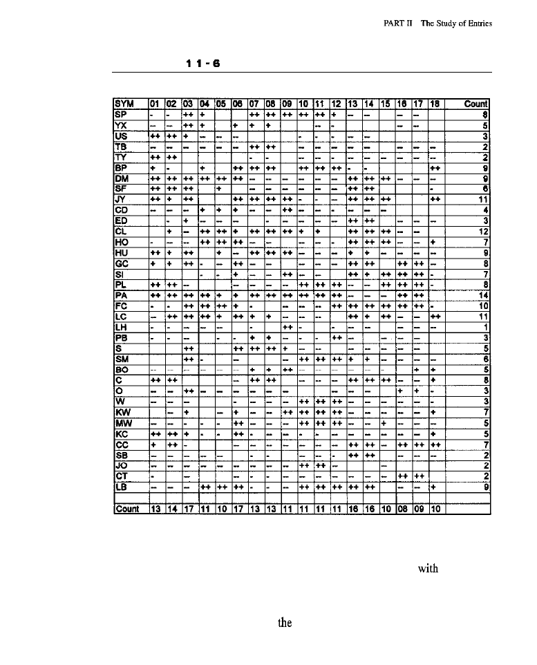
254
T A B L E
Out-of-Sample Results Broken Down by Test and Market
going back further in history, which would be relatively easy to accomplish since
many commodities contracts go back well beyond the start of our in-sample peri-
od (1985). It could also be increased by enlarging the portfolio
additional
markets, perhaps a better way to bolster the training sample.
A maxim of optimization is that the likelihood of performance holding up
increases with reduction in the number of model parameters. Given the somewhat
positive results obtained in some of
tests, it might be worthwhile to experiment
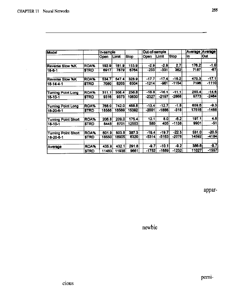
T A B L E 1 1 - 7
Performance of Neural Network Models Broken Down by Model,
Order, and Sample
with more sophisticated models. Specifically, better input preprocessing, in the
sense of something that could reduce the total number of inputs without much loss
of essential predictive information, would probably lead to a very good trading
system. With a smaller number of inputs, there would be fewer parameters (con-
nection weights) in the network to estimate. Consequently, curve-fitting, an
ently significant issue judging by the results and shrinkage levels, would be less of
a problem.
WHAT HAVE WE LEARNED?
n
Under certain conditions, even neural
models can work. The criti-
cal issue with neural networks is the problem of achieving an adequate
ratio of sample size to free parameters for the purpose of minimizing
harmful (as opposed to beneficial) curve-fitting.
n
Curve-fitting is a problem with neural networks. Any methods by which
the total number of parameters to be estimated can be reduced, without
too much loss of predictive information, are worth exploring; e.g., more
sophisticated information-compressing input preprocessing would proba-
bly improve out-of-sample performance and reduce the effects of
curve-fitting.

For similar reasons, large samples are critical to the training of successful
neural network trading models. This is why training on whole portfolios
provides better results than training on individual
despite the
loss of market specificity. One suggestion is to increase the number of
markets in the portfolio and, thereby, achieve a larger in-sample
training
set. Carrying this to an extreme, perhaps a neural network should be
trained on hundreds of commodities, stocks, and various other trading
instruments, in an effort to develop a “universal market forecaster.” If there
are any universal “technical” price patterns that exist in all markets and
that have predictive validity, such an effort might actually be worthwhile.
. Some markets trade poorly, even in-sample. Other markets tend to hold
up out-of-sample. This has been found with other models in earlier chap-
ters: Some markets are more amenable to trading using certain techniques
than are other markets. Selecting a subset of markets to trade, based on
continued out-of-sample performance, might be an approach to take when
developing and trading neural network systems.

C H A P T E R T W E L V E
Genetic Algorithms
E
from models of biology and economics,
gist, John Holland, developed a genetic optimization algorithm and introduced it
to the world in his book, Adaptation in Natural and Artificial Systems (1975).
Genetic algorithms (or
only became popular in computer science about 1.5
years later (Yuret and de la
1994). The trading community first took notice
around 1993, when a few articles (Burke, 1993; Katz and McCormick, 1994;
Oliver, 1994) and software products appeared. Since then, a few vendors have
added a genetic training option to their neural network development shells and a
few have “industrial strength” genetic optimization toolkits.
In the trading community,
never really had the kind of heyday experi-
enced by neural networks. The popularity of this technology probably never grew
due to its nature. Genetic algorithms are a bit difficult for the average person to
understand and more than a bit difficult to use properly. Regardless of their image,
from our experience,
can be extremely beneficial for system developers.
As with neural networks, while a brief discussion is included to provide basic
understanding, it is not within the scope of this book to present a full tutorial on
genetic algorithms. Readers interested in studying this subject further should read
Davis
as well as our contributions to the book
Trading (Katz and
McCormick,
1995b) and our articles (Katz and McCormick, July/August
1994, December 1996, January 1997, February 1997).
WHAT ARE GENETIC ALGORITHMS?
A genetic algorithm solves a problem using a process similar to biological evolution.
It works by the recombination and mutation of gene sequences. Recombination and

mutation are
i.e., they manipulate genes. A gene is a string of
codes (the genotype) that is decoded to yield a functional organism with specific
characteristics (the phenotype). A
chromosome
is a string of genes. In the case of
genetic optimization, as
out on such problems as those being addressed here,
the string of codes usually takes the form of a series of numbers.
During the simulated evolutionary process, a GA engages in mating and
selecting the members of the population (the chromosomes). Mating involves
crossover and mutation. In crossover, the elements that comprise
genes of dif-
ferent chromosomes (members of
population or solutions) are combined to
form new chromosomes. Mutation involves the introduction of random alterations
to
elements. This provides additional variation in the sets of chromosomes
being generated. As with the process of biological selection (where less-fit mem-
bers of the population leave fewer progenies), the less-fit solutions are weeded out
so the more-fit solutions can proliferate, yielding another
that may con-
tain some better solutions than the previous one. The process of recombination,
random mutation, and selection has been shown to be an extremely powerful prob-
lem-solving mechanism.
EVOLVING RULE-BASED ENTRY MODELS
What would happen if a GA were allowed to search, not merely for
best para-
meters (the more common way a GA is applied by traders), but also for the best
rules? In
chapter, the consequences of using a
to evolve a complete entry
model, by discovering both the rules
and
the optimal parameters for those rules,
will be explored. Although somewhat complex,
methodology proved to be
effective in our first investigation (Katz and McCormick, February 1997).
How can a GA be used to discover great trading rules? The garden variety
GA just juggles numbers. It is necessary to
a way to map sets of numbers in
a one-to-one fashion to sets of rules. There
many ways this can be accom-
plished. A simple and effective method involves the construction of a set of rule
templates. A
is a partial specification for a rule, one that contains
blanks that need to be filled in. For example, if some of the rules in previous chap-
ters were regarded as rule templates, the blanks to be filled in would be the values
for
look-backs, thresholds, and other parameters. Using rule templates, as
defined in this manner, a one-to-one mapping of sets of numbers to fully specified
rules can easily be achieved. The first number (properly scaled) of any set is used
as an index into a table of rule templates. The remaining numbers of
set are
then used to fill in the blanks, with the result being a fully specified rule. The code
below contains a C+ + function (Rules) that implements this mapping strategy; it
will be discussed later. Although C+ was used in the current study, this method
can also be implemented in
using the TS-EVOLVE software from
Scientific Consultant Services (516-696-3333).

The term
genetic search
applies to the use of a genetic algorithm to search
through an incredibly large set of potential solutions to find those that are best, i.e.,
that have the greatest fitness. In the current application, the intention is to use the
evolutionary process to discover sets of numbers (genotypes) that translate to
based entry models (phenotypes) with the greatest degree of fitness (defined in
terms of desirable trading behavior). In short, we are going to attempt to engage
in the selective breeding of rule-based entry methods! Instead of beginning with a
particular principle on which to base a model (e.g.,
breakouts, etc.),
the starting point is an assortment of ideas that might contribute to the develop-
ment of a profitable entry. Instead of testing these ideas one by one or in combi-
nations to determine what works, something very unusual will be done: The
genetic process of evolution will be allowed to breed the best possible entry model
from the raw ideas.
The GA will search an extremely broad space of possibilities to find the best
rule-based entry model that can be achieved given the constraints imposed by the
rule templates, the data, and the limitation of restricting the models to a specified
number of rules (to prevent curve-fitting). To accomplish this, it is necessary to
find the best sets of numbers
(those that
map to the best sets of rule-based entry
models) from an exceedingly large universe of possibilities. The kind of massive
search for solutions would be almost impossible-certainly impractical, in any
realistic sense-to accomplish without the use of genetic algorithms. There are
alternatives to
e.g., brute force searching may be used, but we do not have
thousands of years to wait for the results. Another alternative might be through the
process of
induction,
i.e., where an attempt is made to infer rules from a set
of observations; however, this approach
would
not necessarily allow a complex
function, such as that of the risk-to-reward ratio of a trading model, to be maxi-
mized. Genetic algorithms provide an
way to accomplish very large
searches, especially when there are no simple problem-solving heuristics or tech-
niques that may otherwise be used.
E V O L V I N G A N E N T R Y M O D E L
In this exercise, a population of three-rule entry models are evolved using
a C+ + genetic optimizer (Scientific Consultant Services,
3333). Each gene corresponds to a block of four numbers and to a rule, via the
one-to-one mapping of sets of numbers to sets of rules. Each chromosome con-
tains three genes. A chromosome, as generated by the GA, therefore consists of 12
numbers: The first four numbers correspond to the first gene (or rule), the next
four correspond to the second gene (or rule), and the last four correspond to the
third gene (or rule). The GA itself has to be informed of the gene size so it does
not break up intrinsic genes when performing crossover. Crossover should only
occur at the boundaries
of genes,
four number blocks. In the current example,

this will be achieved by setting the “chunk size,” a property of the genetic opti-
mizer component, to four.
As mentioned, each gene is composed of four numbers. The
number is
more than an index into a table of possible rule templates. For example, if
that number is 1, a price-comparison template in which the difference between two
closing prices is compared with a threshold (see code) is selected. The remaining
three numbers in the gene then control the two
periods for the prices being
compared and the threshold. If the first number of the four-number block is 2, a
price-to-moving-average comparison template would be selected. In that case, two
of the remaining
numbers would control the period of the moving average and
the direction of the comparison (whether the price should be above or below the
moving average). In general, if the first number in the block of four numbers that
represents a gene is then the
template is used, and any required parame-
ters are determined by reference to the remaining three numbers in the four-number
block. This decoding scheme makes it easy to maintain an expandable database of
rule templates. Each of the three blocks of four numbers is mapped to a corre-
sponding rule. For any
chromosome, a 3-rule entry model is produced.
The Rule Templates
The
rule template (case I in function Rules) defines a comparison between
two prices and a threshold: The rule takes on a value of TRUE if the closing price
bars ago is greater than some threshold factor
plus the closing price
bars ago. Otherwise, the rule takes on the value of FALSE. The unknowns
and
are left as the blanks to be tilled in during instantiation. This template
has been included because the kind of rule it represents was useful in previous
investigations.
The second rule template (case 2) involves simple moving averages, which
are often used to determine trend. Usually the market is thought to be trending up
if the price is above its moving average and trending down if the price is below its
moving average. There are only two unknowns in this template: The
controls the number of bars in the moving average, and the second
controls
the direction of comparison (above or below).
The third rule template (case 3) is identical to the second
except that
an exponential moving average is used rather than a simple moving average.
Much discussion has occurred regarding the importance of open interest.
Larry Williams (1979) mentioned that a decline in total open interest, during a
period when the market has been moving sideways, indicates potential for a strong
rally. A shrinking of open interest may be interpreted as a decline in available con-
tracts, producing a condition where demand may outweigh supply. The fourth rule
template (case 4) simply computes the percentage decline in open interest from
bars ago to 1 bar ago (open interest is generally not available for the current
7.61
bar) and compares it with a threshold
If the percentage decline is greater than
the threshold,
the rule
takes on
the
value
TRUE.
Otherwise it evaluates to
FALSE.
The threshold and the
are the unknowns to be tilled in at the time
of instantiation.
The fifth rule template
5) is similar to the fourth template, but a rise,
rather than fall, in total open interest is being sought. If the increase, as a percent-
age, is greater than a threshold, then the rule evaluates to
TRUE.
Otherwise it eval-
uates to
FALSE.
As previously, the
and the threshold are unknowns
must he supplied to instantiate
rule.
The sixth rule template (case can be called a “new high” condition: The
template asks whether an
new high has occurred within the last
lb2
bars.
A particular instance of the rule might read: “If a new
high has occurred
within the last 10 days, then
TRUE,
else
FALSE.”
This rule attempts to capture a
simple breakout condition, allowing for breakouts
may have occurred several
bars ago (perhaps followed by a pull-back to the previous resistance-turned-sup-
port that another rule has detected as a good entry point). There are two blanks to
be tilled in to instantiate this template:
and
lb2.
The seventh rule template (case is identical to the sixth rule template,
except
new lows, rather than new highs, are being detected.
The eighth rule template (case 8) examines the average directional move-
ment index with respect to two thresholds
and
This is a measure of
trendiness, as discussed in the chapter on breakouts. If the average directional
movement (ADX) is above a lower threshold and below an upper threshold, the
rule evaluates to
TRUE.
Otherwise, the rule evaluates to
FALSE.
The
rule template (case 9) performs a threshold comparison on the
Stochastic oscillator that is similar to
performed in Rule 8.
The tenth rule template (case
evaluates the direction of the slope of the
MACD oscillator. The lengths
and
of the two moving averages that com-
pose the MACD, and
direction of the slope
required for the role to evalu-
ate to
TRUE,
are specified as parameters.
TEST METHODOLOGY
Below are the steps involved in evolving an entry model based on the rule tem-
plates being used in this study:
1. Retrieve a
chromosome from the genetic optimizer compo-
nent. This represents a potential solution, one that initially will be ran-
dom and probably not very good.
2. Instantiate the rule templates to obtain three fully defined
(one for
each gene), and compote their
TRUE/FALSE values
for all bars in the
data series,
upon the decoding of the genes/chromosome.

3. Proceed bar by bar through the data. If, on a given bar, all three instanti-
ated rules evaluate to
TRUE,
and if there is no current long (or short)
position, then post an order to the simulator component to buy (or sell)
at tomorrow’s open.
4. If a position is being held, use the standard exit strategy to handle the
exit.
5. Evaluate the trading performance of the potential solution. For this exer-
cise, the basic “goodness” of a solution is defined as
annualized
to-reward ratio, a figure that is actually a
t-statistic.
6. Tell the genetic optimizer how fit (in the above sense) the potential solu-
tion (the chromosome it provided) was. This allows the genetic optimiz-
er component to update the population of chromosomes it maintains.
7. If the solution meets certain criteria, generate performance summaries
and other information, and save this data to a file for later perusal.
8. Repeat the above steps again and again until a sufficient number of
“generations” have passed.
As the above steps are repeated, the solutions, i.e., the “guesses” (actually, “off-
spring”), provided by the genetic optimizer, will get better and better, on average.
Because of the way the genetic process works, large numbers of distinct, yet effec-
tive, solutions will emerge during the evolutionary process. Most of the solutions
will have been recorded in a tile generated in the course of repeatedly performing
the first seven computational steps. In the “Code” section of this chapter, a dis-
cussion can be found of some of the C++ code that actually implements the
above steps, including the instantiation and computation of the rules.
Because of the nature of the rules, asymmetries are likely. Consequently,
long entry models are evolved and tested separately from short entry models.
Model performance is evaluated on the entire portfolio. The goal is to find a set of
rules that, when applied in the same way to every tradable, produce the best over-
all portfolio performance. The procedure being used here differs from the one in
our earlier investigation (Katz and McCormick, February 1997) where sets of
rules, specific to each of several markets, were evolved, an approach that was
much more subject to the effects of curve-fitting. As observed
several other
models that were originally tested on individual tradables, some performance may
be lost when requiring a common model across all markets without market-spe-
cific optimization or tuning. In the tests that follow, the standard C+ + software
platform, as well as the standard entry orders and exit strategy, are used.
static
Used the Rules
function
to simplify coding
i ;

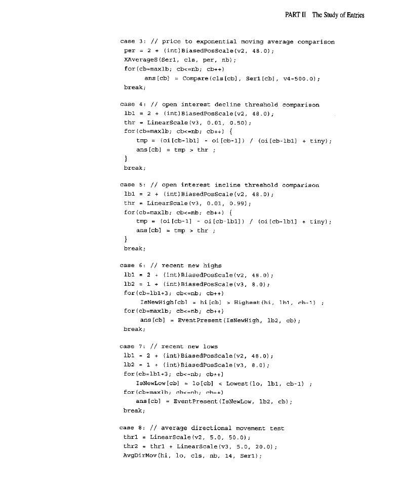

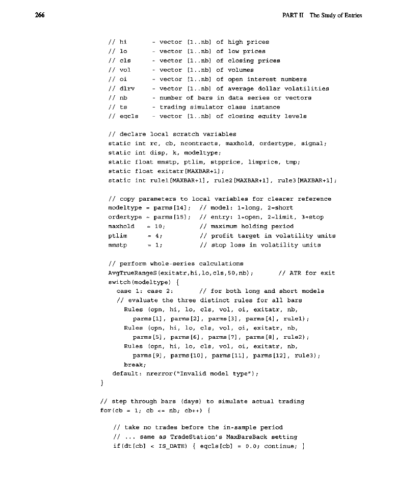


)
process
The
+ code implements the rule templates and system trading strategy. The
function Rules implements the rule templates. Arguments
and
(which correspond to the four numbers that comprise any one of the three genes)
provide all the information required to instantiate a rule template. Argument
is
used to select, via a “switch statement,” the required rule template from the 10 that
are available; arguments
and
are used to till in the blanks (required
parameters, desired directions of comparison, etc.) to yield a fully defined rule.
The rule is then immediately evaluated for all bars, and the evaluations (1 for
TRUE, 0 for FALSE) are placed in
a floating-point vector used to return the
results to the caller.
The macro,
is used to map numbers ranging from 0 to
1,000 to a range of 0 to a, with more numbers mapping to smaller values than
larger ones. The macro is used to compute such things as lookbacks and
average periods from
or
the values of which are ultimately derived
from the genetic algorithm and scaled to range from 0 to 1,000. The macro is non-
linear
(Biased)
so that a finer-grained exploration occurs for smaller periods or
lookbacks than for larger ones. For example, suppose there is a moving average,
with a period that ranges from 2 to 100 bars. The intention is to search as much
between periods 2, 3, and 4 as between 30, 50, and 90; i.e., the scale should be
spread for small numbers. This is desired because, in terms of trading results, the
change from a
moving average to a 5-bar moving average is likely to be
much greater than the change from a
to a
moving average.
The macro,
performs a linear mapping of the range 0
1,000 to the range a b. The macro is usually used when calculating
thresholds or deviations. In the rule template code, all parameters are scaled
inside Rules, rather than inside the GA as is the usual practice. The GA has
been instructed to produce numbers between 0 and 1,000, except for chromo-
some elements 5, and 9, which are the first numbers in each gene, and which
serve as rule template selectors. The reason for local scaling is that templates
for different kinds of rules require parameter and control values having differ-
ent ranges to be properly instantiated.
The process of evolving trading systems involves asking the genetic opti-
mizer to provide a “guess” as to a chromosome. The genetic optimizer then
domly picks two members of the population and mates them (as specified by the
crossover, mutation rate, and chunk-size properties). The resultant offspring is
then returned as a potential solution. When the GA component is told the fitness

of the solution it has just provided, it compares that fitness with that of the
member of the population it maintains. If the fitness of the offspring is greater
than the fitness of the least-fit member, the GA replaces the least-fit member with
the offspring solution. This process is repeated generation after generation, and is
handled by the shell code (not shown), which, in turn, makes repeated calls to
function Model to simulate the trading and evaluate the system’s fitness.
The code for function
Model
is almost identical to that used in earlier chap-
ters. Prior to the bar indexing loop in which trading orders are generated, the func-
tion
is invoked three times (once for each gene), with the results being
placed in time series
and
A
average true range is also
calculated, as it is necessary for the standard exit and for rule evaluation. Inside
the loop, the rule evaluations are checked for the current bar
and if all evaluations are
TRUE, a
buy (or a sell, if the short side is
being examined) is generated. Entries are programmed in the standard manner for
each of the three orders tested. Only the in-sample data is used to in the evolu-
tionary process.
The output produced by the shell program permits the selection of desirable
solutions that may be traded on their own or as a group. The solutions may be eas-
ily translated into understandable rules to see if they make sense and to use as ele-
ments in other systems.
TEST RESULTS
Six tests were performed. The evolutionary process was used to evolve optimal
entry rules for the long and short sides with each of the three entry orders: at open,
on stop, and on limit. In all cases, a maximum of 2,500 generations of genetic pro-
cessing was specified. The task of computing all
solutions and saving them to
tiles took only a few hours on a fast
which demonstrates the practicality
of this technique. For each test, the genetic process produced a tabular file
1 through 6) consisting of lines corresponding to each of
generations; i.e., each
line represents a specific solution. Most of the early solutions were close to ran-
dom and not very good, but the quality of the solutions improved as generations
progressed; this is normal for a GA. Each line contains information regarding the
performance of the particular solution that corresponds to the line, as well as to the
complete chromosome, i.e., the set of parameters that represents the gene, which,
in turn, corresponds to the solution expressed in the line.
The best solutions for the long entry at open and for
short entry at open
were selected. These solutions were used to generate the six tests conducted
below. More specifically, the solution that provided the best long entry at open was
tested and its performance was evaluated in the usual way on both samples. The
same solution was also tested and evaluated with entry on stop and on limit. The
same procedure was followed for the short side: The best evolved solution for a
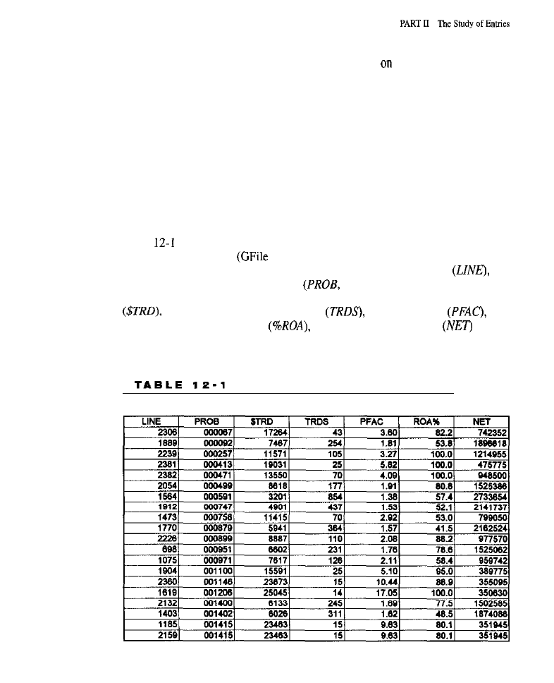
270
short entry at open was determined. It was then tested
both samples with each
of the other two order types, The optimal solution for each order type was not
selected separately from our genetic runs because doing so would not allow com-
parability across orders. For example, the optimal entry at open might involve a
breakout, while the optimal entry for a stop might involve countertrend momen-
tum-totally different models. By assuming that the entry-at-open model (in
which all trades generated by the model are taken) represents a good, overall
model, the normal course of evaluating that model with the other orders was fol-
lowed. Since the model is kept constant, this approach permits meaningful com-
parisons to be made across orders.
Solutions Evolved for Long Entries
Table
furnishes some of the performance data for the top 20 solutions for
long entries at the open
1). Each line represents a different trading model.
The parameters are not shown, but the line or generation number
the
probability or statistical significance
the decimal point is omitted but
implied in the formatting of these numbers), the average dollars-per-trade
the total number of trades taken
the profit factor
the
annualized return-on-account
and the net profit or loss
in raw
numbers are provided.
The Top 20 Solutions Evolved for Long Entries at the Open
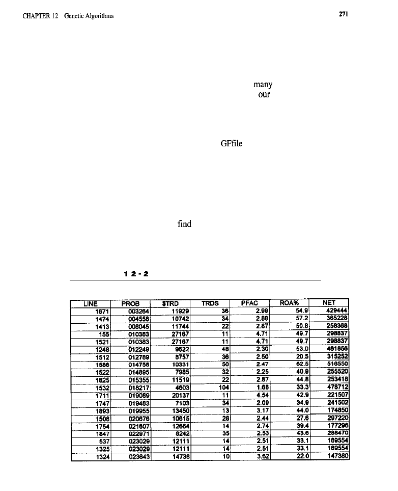
The performance of most of these models is nothing short of impressive. The
better models are statistically significant beyond the 0.00007 level, which means
these solutions have a very high probability of being real and holding up in the
future. Many of the returns were greater than 50% annualized. In some cases, they
reached much higher levels. While the limit order had
of the best solutions,
all orders had many good, if not great, solutions. As in
earlier study, the GA
succeeded admirably in finding many tradable models.
Solutions Evolved for Short Entries
Table 12-2 provides a small proportion of
4, the file for evolved models
generated for short entries at the open. As in Test 1, the top 20 solutions, in terms
of statistical significance or risk-to-reward ratio, are presented. Again, it can be
seen that there were many good solutions. However, they were not as good as
those for the longs. The solutions were not as statistically significant as for the
longs, and the return-on-account numbers were somewhat smaller. A somewhat
more distressing difference is that, in most cases, the number of trades was very
small; the models appear to have been picking rare events. All else aside, the evo-
lutionary process was able to
numerous, profitable rule sets for the short
entries.
T A B L E
The Top 20 Solutions Generated for Short Entries at the Open

Test Results for the Standard Portfolio
The best solution shown in Table 12-1 (long trades)
the best solution from
Table 12-2 (short trades)
with all three entry orders. Tests 1 through 3
represent the best evolved model for long entry at the open tested with entry at
open, on limit, and on stop (respectively). Tests 4 through 6 represent the best
evolved model for short entry over all three orders. Table 12-3 contains the per-
formance data for the best evolved entry-at-open models, both long
short, on
the optimization
verification samples using each of the three entry orders. In
the table,
= whether the test was on the optimization sample
(IN or OUT);
ROA%
the annualized return-on-account;
= the annualized
reward ratio:
PROB
the associated probability or statistical significance;
TRDS
the number of
trades
taken across all commodities in the portfolio;
WZN% =
the
percentage of winning trades;
$TRD =
average profit/loss per trade;
BARS = the
T A B L E
Performance of the Best Evolved Entry-at-Open Model on the
and Verification Samples with Each of the Three Entry
I
I
Test
Short entry-at-open
entry on stop
IN
23.11
0.0311
OUT
3 0

average number of days a trade was held, NETL = the total net profit on long
trades, in thousands of dollars; and NETS = the total net profit on short trades, in
thousands of dollars.
Tests 1 through 3: Long-Entry-At-Open Model Tested with Entry at Open, on
Limit,
and
on
Stop.
As can be seen in Table 12-3, the entry model produced by
the evolutionary process was profitable across all three order types, both in-sam-
ple (as would be expected given the optimization power of
and out-of-sam-
ple. In-sample, no return was less than 42% (annualized) for any order. The
dollars-per-trade figures were all greater than $14,000, and not one system had
less
60% wins! Out-of-sample, there was
variation. With entry at open
and on limit, performance continued to be stellar, with the average trade above
$10,000 and
return on account above 60%. With a stop order, performance was
not quite as good: The return on account was only 11%, and the average trade
yielded $4,246. The only distressing aspect of the results is the small number of
trades taken. For example, in-sample, with entry at open, there were only 43 trades
taken over a lo-year span on a portfolio of 36 commodities. Out-of-sample, there
were only 17 trades over a
period; the trading frequency was roughly con-
stant at approximately 4 trades per year.
The rules were apparently detecting unusual (but tradable) market events; the
model engaged in what might be termed “rare event trading,” which is not neces-
sarily a bad thing. An assortment of systems, each trading different rare events,
could yield excellent profits. When working with a system such as this, trading a
portfolio of systems, as well as a portfolio of commodities, would be suggested.
In the current situation, however, few trades would place the statistical reliability
of the findings in question. The entire problem can be dealt with by using a some-
what
complex way of handling larger combinations of rules.
Tests 4 through 6: Short-Entry-at-Open Model Tested on Entry at Open, on
Limit, and on Stop.
In all cases, the performance of the best evolved short entry
at open model, when tested over the three order types, was poorer on the in-sample
data than the long model. Out-of-sample, the results deteriorated significantly and
losses occurred. Unlike the long model, this one did not hold up. It should be noted,
however, that if both the long and short models had been traded together on
sample data, the profits from the long side would have vastly outweighed the loss-
es from the short side; i.e., the complete system would have been profitable. The
pattern of longs trading better than shorts is a theme that has been recurrent
throughout the tests in this book. Perhaps the pattern is caused by the presence of
a few markets in the standard portfolio that have been in extreme bullish mode for
a long time. The way commodities markets respond to excess supply, as contrasted
to the way they respond to shortages, may also help explain the tendency.
Market-by-Market Test Results
Table 12-4 contains the market-by-market results for the best evolved
open models, both long and short, tested on the optimization and verification
samples using each of the
entry orders. Given the small number of trades
taken, many of the empty cells in this table simply reflect the absence of trades.
The
column represents the market being studied. The center and rightmost
columns
contain the number of profitable tests for a given market. The
numbers in the first row represent test identifiers:
01,
02, and 03 represent tests
with entry at open, on limit, and on stop, respectively, for the long side; 04, 05,
and 06 represent corresponding tests for the short side. The last row
contains the number of markets on which a given model was profitable. The data
in this table provides relatively detailed information about which markets are and
are not profitable when traded by each of the models: One dash (-) indicates a
moderate loss per trade, i.e., $2,000 to $4,000; two dashes
represent a large
loss per trade, i.e., $4,000 or more; one plus sign (+) means a moderate profit per
trade, i.e., $1,000 to
two pluses (+ +) indicate a large gain per trade, i.e.,
$2,000 or more; and a blank cell means that the loss was between $0 and $1,999
or the profit was between $0 and $1,000 per trade. (For information about the
ious markets and their symbols, see
II-1 in the “Introduction” to Part II.)
Tests 1 through 3:
Model Tested on Entry Open, on Limit,
and
on
Table 12-4 indicates that, in-sample,
model was strongly profitable
for the
(but not the S&P
British Pound, the
the
Japanese Yen, Palladium, most of the Wheats, Kansas Wheat, Cocoa, and Lumber,
and Light Crude (if entry at open is omitted). Out-of-sample, the
had no
trades, the British Pound and the Deutschemark continued to be strongly profitable
across all three order types, and many of the other markets in which strong in-sample
profitability was observed had no trades. Out-of-sample, some markets that had not
traded in-sample traded profitably (especially Unleaded Gasoline, Silver, and
Coffee), which indicates that the model continued to perform well, not merely in a
different time period, but on a different set of markets.
4 through 6:
Tested on Entry at Open, on Limit,
and on
In-sample, the T-Bills, the
the Swiss Franc, the
Canadian Dollar, Pork Bellies, Oats, Kansas Wheat, Orange Juice, and Lumber all
showed strong profits. The British Pound and
held up out-of-sample.
The Swiss Franc was profitable out-of-sample, hut only with
limit order. It lost
when entry was at open or on stop. The other markets either did not trade out-of-sam-
ple or had losses. Out-of-sample, the
traded strongly profitably across all
order types, but did not trade profitably in-sample.
Figure 12-1 depicts portfolio equity growth for long trades taken
entry
at open. As is evident, there was a steady, stair-like
in equity, the stair-like
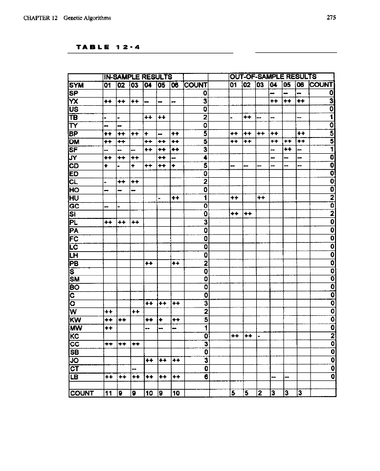
Breakdown of Performance By Market and Test
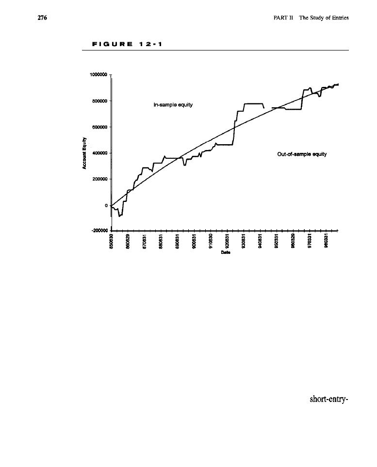
Portfolio Equity Growth for Long Model with Entry at the Open
quality resulting from the small number of trades taken. The occasional, strongly
profitable trade caused a sudden step up in equity. The least-squares line fitted to
the equity curve reveals consistent growth in both samples, but slightly greater in
the early years.
The equity growth for the long model with entry on limit, which helps to
control transaction costs, is shown in Figure 12-2. Again, the stair-like growth
in equity is apparent. However, the equity growth was more even; i.e., there was
no slowing down of growth in recent year-in fact, the fitted line is almost
straight. Out-of-sample performance was almost identical to in-sample perfor-
mance.
Figure 12-3 shows portfolio equity growth for the best evolved
at-open model, evaluated with entry actually at the open. Again, the stair-like
appearance is present. However, except for a strong spurt of growth between
August 1989 and June 1993, the curve is essentially flat. Overall, the equity was
seen rising, except for the flat regions.
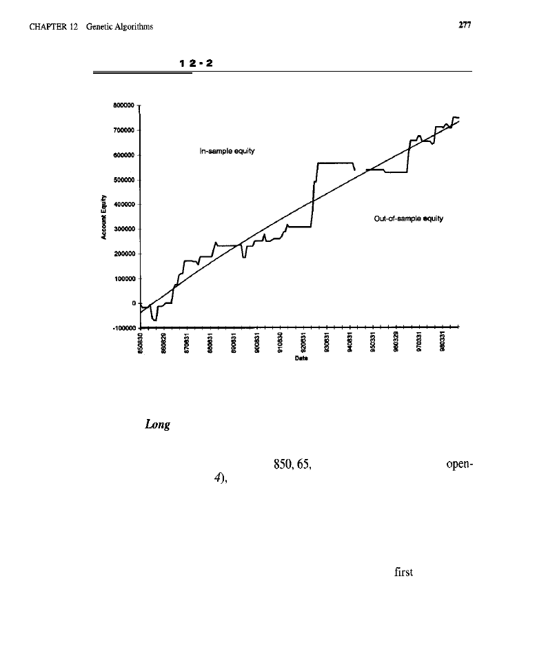
F I G U R E
Portfolio Equity Growth for Long Model with Entry on a Limit
The Rules for the Solutions Tested
Rules
for
Entry.
The chromosome that represented the best solution for
long entries at the open contained three genes. Each gene was composed of four
numbers and corresponded to a specific rule.
The numbers for Gene 1 were 4,
and 653, which specified an
interest decline rule (case
a look-back of 34, and a threshold of 0.042, respec-
tively. The last number (653) was not used or translated because the rule did not
require three blanks to be filled in, only two. If this information is taken and trans-
lated into plain language, the rule says that the open interest must decline at least
4.2% over
the past
34
bars for the rule to evaluate
as TRUE.
In other words, the
open interest 34 bars ago (relative to the current bar) minus the open interest 1 bar
ago, divided by the open interest 34 bars ago, was greater than 0.042.
The numbers for Gene 2 were 1, 256, 530, and 709. The
number (1)
specified a simple price comparison mle (case I). When the additional numbers
were translated to the correct lookbacks and thresholds,
it
is apparent that this rule
fires (evaluates as
TRUE)
when the close 3 days ago is greater than the close 14
days ago plus 3.46 times the average true range.
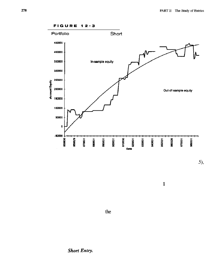
Equity Growth for
Model with Entry at the Open
The numbers for Gene 3 were 5, 940, 47, and 610. Rule template 5 (case
which is the open-interest incline rule, was specified by the first number. Fully
instantiating this rule reveals that the rule evaluates as
TRUE
if the market’s open
interest has risen at least 5.6% in the past 44 days.
If the conditions for all three rules, specified by Genes through 3, were met
on a given bar, a buy signal was generated.
It is interesting that two rules involved open interest, a variable not usually con-
sidered in many popular approaches to trading. It is also noteworthy that the two
open-interest rules, when put together, seem almost contradictory: The current open
interest had to be greater than
open interest 44 bars ago, but less than the open
interest 34 bars ago. The model appears to be somewhat trend-following in that a
recent closing price had to be greater than an older closing price before an entry was
taken. However, time was left for a small pull-back; i.e., the increase in price only had
to be observed 3 bars ago, not in the current bar. The set of rules is not one that would
be easy to discover in a normal manner, without the aid of a genetic algorithm.
Rules
for
A similar analysis can be done for the shorts as for the
longs. The numbers corresponding to the chromosome that represented the best

solution for short entries at the open were 5, 890, 391, and 532 (Gene 1); 5,705,
760, and 956 (Gene 2); and
163,999, and 196 (Gene 3). When the string of
three genes was translated, it was revealed that two rules deal with open interest
and one with the MACD oscillator. The first open-interest role states that the
open interest 1 bar ago must be at least 38% greater than the open interest 38
bars ago. The second open-interest rule states that the open interest 1 bar ago
must be at least 75% greater than the open interest 25 bars ago. The third rule
states that the slope of the MACD-with a shorter moving average length of 2
and a longer moving average length of
be down, suggesting a current
downward trend. If the conditions for all three rules, specified by the three
genes, were met on a given bar, a sell signal was generated. Again, these rules
would not have been easily discovered when developing a trading model in a
more traditional manner.
CONCLUSION
As was the case in our earlier study, the use of a GA to select and instantiate rule
templates continued to work well as a means of developing a trading system, or,
at least, an entry model. Results were still impressive, despite such problems as
inadequate numbers of trades in many of the solutions generated. The approach is
certainly one that can serve as the basis for further development efforts. In this
exercise, only a small base of rule templates, involving such fairly simple elements
as price comparisons, moving averages, and indicators, were used. Undoubtedly,
much better results could be obtained by using a more sophisticated and complete
set of role templates as grist for the genetic mill.
WHAT HAVE WE LEARNED?
. Long positions tend to perform better than short positions for the markets
in our standard portfolio and with the models that were tested. Therefore,
it is probably more worthwhile to place development efforts on a system
that emphasizes the long rather than short side.
. Genetic algorithms appear to be an effective means of discovering small
inefficiencies that are buried in a mountain of efficient market behaviors.
n
When used correctly, and in such a manner as discussed above,
(curve-fitting) does not seem to be a serious problem, despite
the optimization power of genetic algorithms. Restrictions on the number
and complexity of the rules in any solution seems to be the key element
in controlling the curve-fitting demon.
. Evolution, as used herein, has the great benefit of producing explicit rules
that can be translated into plain language and understood. Unlike neural

network systems, the trading rules produced by
are not hidden in an
inscrutable black box.
. Using genetics in the manner described above has the benefit of produc-
ing a large number of distinct, yet profitable, solutions. It would be easy
evolve and then put together a portfolio of systems.

P A R T T H R E E
T H E S T U D Y O F E X I T S
Introduction
n Part II, the focus was on the timing of trade entries. The extent to which various
methodologies are useful in the process of deciding when, where, and how to enter
a trade was examined. Tests were conducted on everything from cycles to sunspot
activity, from simple rule-based approaches to advanced genetic algorithms and
neural networks. In order that a reasonably fair comparison of entry methods could
be made, the exit strategy was intentionally kept simple and constant across all
tests. A fixed money management stop, a profit target limit, and an exit at market
after a given number of bars, or days, in the trade were used. In Part III, attention
will be shifted to the problem of how to get out of a trade once in, i.e., to exit strate-
gies, an issue that has often been neglected in the trading literature.
THE IMPORTANCE OF THE EXIT
In many ways, a good exit is more critical and difficult to achieve than a good entry.
The big difference is that while waiting for a good opportunity to enter a trade, there
is no market risk. If one opportunity to enter is missed, another will always come
along-and a good, active trading model should provide many such opportunities.
When a trade is entered, however, exposure to market risk occurs simultaneously.
Failing to exit at an appropriate moment can cost dearly and even lead to the dread-
ed margin call! We actually know someone who made a quick, small fortune trad-
ing, only to lose it all (and then some) because the exit strategy failed to include a
good money management stop! To get out of a trade that has gone bad, it is not a
good idea to simply wait for the next entry opportunity to come along. Similarly,
erring on the side of safety and exiting at the drop of a hat can also drain a trading

account, albeit less dramatically through slow attrition. The problem with frequent
and hasty exits is that many small losses will occur due to the sacrifice of many
potentially profitable trades, and trades
are profitable will be cut short before
reaching their full profit potential. A good exit strategy must, above all, strictly con-
trol losses, but it must not sacrifice too many potentially profitable trades in the
process; i.e., it should allow profitable trades to fully mature.
How important is the exit strategy? If risk can be tightly controlled by quick-
ly bailing from losing trades, and done in such a way that most winning trades
not killed or cut short, it is possible to turn a losing system into a profitable one!
It has been said that if losses are cut short, profits will come. A solid exit strategy
can, make a profitable system even more lucrative, while reducing equity volatili-
ty and drawdown. Most importantly, during those inevitable bad periods, a good
exit strategy that incorporates solid money management and capital preservation
techniques can increase the probability that the trader will still be around for the
next potentially profitable trade.
GOALS OF A GOOD EXIT STRATEGY
There
two goals that a good exit strategy attempts to achieve. The first and
most important goal is to strictly control losses. The exit strategy must dictate how
and when to get out of a trade that has gone wrong so that a significant erosion of
trading capital can be prevented. This goal is often referred to as
manage-
and is frequently implemented using stop-loss orders (money management
stops). The second goal of a good exit strategy is to ride a profitable trade to full
maturity. The exit strategy should determine not only when to get out with a loss,
but also when and where to get out with a profit. It is generally not desirable to
exit a trade prematurely, taking only a small profit out of the market. If a trade is
going favorably, it should be ridden as long as possible and for as much profit as
reasonably possible. This is especially important if the system does not allow mul-
tiple reentries into persistent trends. “The trend is your friend,” and if a strong
trend to can be ridden to maturity, the substantial profits that will result can more
than compensate for many small losses. The protit-taking exit is often implement-
ed with trailing stops. profit targets, and time- or volatility-triggered market
orders. A complete exit strategy makes coordinated use of a variety of exit types
to achieve the goals of effective money management and profit taking.
KINDS OF EXITS EMPLOYED IN AN EXIT
STRATEGY
There are a wide variety of exit types to choose from when developing an exit
strategy. In the standard exit strategy, only three kinds of exits were used in a sim-
ple, constant manner. A
fixed
money management
was implemented using a
stop order: If the market moved against the trade more than a specified amount.

the position would be stopped out with a limited loss. A
exit was
implemented using a limit order: As soon as the market moved a specified amount
in favor of the trade, the limit would be hit and an exit would occur with a known
profit. The time-based
was such that, regardless of whether the trade was prof-
itable, if it lasted more than a specified number of bars or days, it was closed out
with an at-the-market order.
There are a number of other exit types not used in tbe standard exit strategy:
trailing exits, critical threshold exits, volatility exits, and signal exits. A trailing
exit, usually implemented with a stop order and, therefore, often called a trail-
ing
may be employed when the market is moving in favor of the trade. This
stop is moved up, or down, along with the market to lock in some of the paper
profits in the event that the market changes direction. If the market turns against
the trade, the trailing stop is hit and the trade is closed out with a proportion of
the profit intact. A critical threshold exit terminates the trade when the market
approaches or crosses a theoretical barrier (e.g., a trendline, a support or resis-
tance level, a Fibonacci
or a Gann line), beyond which a change in
the interpretation of current market action is required. Critical threshold exits
may be implemented using stop or limit orders depending on whether the
trade
is long or short and whether current prices are above or below the barrier level.
If market volatility or risk suddenly increases (e.g., as in the case of a “blow-off
top), it may be wise to close out a position on a volatility exit. Finally, a
signal
exit is simply based on an expected reversal of market direction: If a long posi-
tion is closed out because a system now gives a signal to go short, or because an
indicator suggests a turning point is imminent, a signal exit has been taken.
Many exits based on pattern recognition are signal exits.
Money Management Exits
Every exit strategy must include a money
management
A money management
exit is generally implemented using a stop order. Therefore, it is often referred to
as a money management stop. Such a stop closes out a trade at a specified amount
of adverse excursion (movement against the trade), or at a specified price below
(if long) or above (if short) the price at which the trade was entered. A money man-
agement stop generally stays in place for the duration of the trade. Its purpose is
to control the maximum risk considered tolerable. Of course, the potential risk
may be greater than what was expected. The market
could
go limit up (or down)
or have a large overnight gap. Trading without a money management stop is like
flying in a rickety old plane without a parachute,
The issue is not whether a money management stop should be used. Rather,
it is determining the optimal placement of the stop. There are many ways to decide
where to place money management stops, The simplest placement occurs by
assessing the maximum amount of money that can be risked on a given
trade.
For

example, if a trade on the S&P 500 is entered and the trader is not be willing to
risk more than $1,500, a money management stop that uses a $1,500 stop-loss
order would be specified. If the market moves against the trade more than $1,500
(three S&P points), the stop gets hit and the position is closed out. Another way to
set the money management stop is on the basis of volatility. In volatile markets and
periods, it may be a good idea to give trades more room to breathe, i.e., to avoid
having the stop so close to the market that potentially profitable trades get stopped
out with losses.
A good way to set a money management stop is on the basis, of a price bar-
rier, such as a trendline or support/resistance level. In such cases, the stop also
serves as a critical threshold exit. For example, if there are a number of trend and
support lines around 936.00 on the S&P 500, and a long position at 937.00 has just
been entered, it might be worth considering the placement of a stop a little below
936.00, e.g., at 935.50. Setting a protective stop at 935 is logical since a break
through support suggests that the trend has changed and that it is no longer smart
to be long the S&P 500. In this example, only $750 is at risk, substantially less
than the $1,500 risked when using the money management stop that was based on
a dollar amount. A tighter stop can often be set using a barrier or critical price
model than would be the case using a simple dollar-amount model.
As hinted above, setting a money management stop involves a compromise. It
is good to have a very tight stop, since losing trades then involve only tiny, relatively
painless losses. However, as the stop is
(i.e., moved closer to the entry or
current price), the likelihood of it getting triggered increases, even if the market even-
tually moves in favor of the trade. For example, if a $50 stop loss is set,
trades on the S&P 500, regardless of entry method, will be stopped out with small
losses. As a stop gets tighter, the percentage of winning trades will decrease. The stop
eventually ends up sacrificing most of what would have been profitable trades. On the
other hand, if the stop is too loose, although the winning trades are retained, the
adverse excursion on those winners, and the losses on the losing trades, will quickly
become intolerable. The secret is to find a stop that effectively controls losses with
out sacrificing too many of the trades that provide profits.
Trailing Exits
A
exit is usually implemented with a so-called trailing stop. The purpose
behind this kind of exit is to lock in some of the profits, or to provide protection
with a stop that is tighter than the original money management stop, once the mar-
ket begins to move in the trade’s favor. If a long position in the S&P 500 is taken
and a paper profit ensues, would it not be desirable to preserve some of that prof-
it in case the market reverses? This is when a trailing stop comes in useful. If a
$1,500 money management stop is in place and the market moves more than
$1,500 against the trade, the position is closed
a $1,500 loss. However, if the

market moves $1,000 in the trade’s favor, it might be wise to move the old money
management stop closer to the market’s current price, perhaps to $500 above the
current market price. Now, if the market reverses and the stop gets hit, the trade
will be closed out with a $500 profit, rather than a $1,500 loss! As the market
moves further in favor of the trade, the trailing stop can be moved up (or down, if
in a short position), which is why it is called a trailing stop, i.e., it is
up
(or down), trailing the market-locking in more of the increasing paper profit.
Once it is in place, a good trailing stop can serve both as an adaptive money
management exit and as a profit-taking exit, all in one! As an overall exit strategy,
it is not bad by any means. Trailing stops and money management stops work hand
in hand. Good traders often use both, starting with a money management stop, and
then moving that stop along with the market once profits develop, converting it to
a trailing stop. Do not be concerned about driving the broker crazy by frequently
moving stops around to make them trail the market. If trading is frequent enough
to keep commissions coming in, the broker should not care very much about a few
adjustments to stop orders. In fact, a smart broker will be pleased, realizing that
his or her client is much more likely to survive as an active, commission-produc-
ing trader, if money management and trailing stop exits are used effectively.
How is the placement of a trailing stop determined? Many of the same prin-
ciples discussed with regard to money management exits and stops also apply to
trailing exits and
The stop can be set to trail, by a fixed dollar amount, the
highest (or lowest, if short) market price achieved during the trade. The stop can
be based on a volatility-scaled deviation. A moving threshold or barrier, such as a
trend or
line, can be used if there is one present in a region close enough to
the current market action. Fixed barriers, like support/resistance levels, can also be
used: The stop would be jumped from barrier to harrier as the market moves in the
trade’s favor, always keeping the stop comfortably trailing the market action.
Profit Target Exits
A
is usually implemented with a limit order placed to close out a
position when the market has moved a specified amount in favor of the trade. A
limit order that implements a profit
exit can either be fixed, like a money
management stop, or be moved around as a trade progresses, as with a trailing
stop. A fixed profit target can be based on either volatility or a simple dollar
amount. For example, if a profit target of $500 is set on a long trade on the S&P
500, a sell-at-limit order has been placed: If the market moves $500 in the trade’s
favor, the position is immediately closed. In this way, a quick profit may be had.
There are advantages and disadvantages to using a profit target exit. One
advantage is that, with profit target exits, a high percentage of winning trades can
be achieved while slippage is eliminated, or even made to work in the trader’s
favor. The main drawback of a profit target exit is that it can cause the trader to

prematurely exit from large, sustained moves, with only small profits, especially
if the entry methods do not provide for multiple reentries into ongoing trends. All
things being equal, the closer the profit target is to the entry price, the greater the
chances are of it getting hit and, consequently, the higher the percentage of win-
ning trades. However, the closer the profit target, the smaller the per-trade profit.
For instance, if a $50 profit target is set on a trade in the S&P 500 and the money
management stop is kept far out (e.g., at
more than 95% of the trades will
be winners! Under such circumstances, however, the wins will yield small profits
that Will certainly be wiped out, along with a chunk of principal, by the rare $5,000
loss, as well as by the commissions. On the other hand, if the profit target is very
wide, it will only occasionally be triggered, but when it does get hit, the profits
will be substantial. As with exits that employ stops, there is a compromise to be
made: The profit target must be placed close enough so that there can be benefit
from an increased percentage of winning trades and a reduction in slippage, but it
should not be so close that the per-trade profit becomes unreasonably small. An
exit strategy does not necessarily need to include a profit target exit. Some of the
other strategies, like a trailing stop, can also serve to terminate trades profitably.
They have the added benefit that if a significant trend develops, it can be ridden to
maturity for a very substantial return on investment. Under the same conditions,
but using a profit target exit, the trade would probably be closed out a long time
before the trend matures and, consequently, without capturing the bulk of the prof-
it inherent in the move.
Personally, we prefer systems that have a high percentage of winning
trades.
Profit targets can increase the percentage of wins. If a model that is able to reen-
ter active trends is
used,
profit target exits may be effective. The advantages and
disadvantages really depend on the nature of the system being trading, as well as
on personal factors.
One kind of profit target we have experimented with, designed to close out
dead, languishing trades that fail to trigger other types of exits, might be called a
A profit target that is very far away from the market is set.
Initially, it is unlikely to be triggered, but it is constantly
moved
closer and closer
to where the market is at any point in the trade. As the trade matures, despite the
fact that it is not going anywhere, it may be possible to exit with a small
when the profit target comes into a region where the market has enough volatility
to hit it, resulting in an exit at a good price and without slippage.
Time-Based Exits
Time-based
involve getting out of the market on a market order after having
held a trade for a
period of time. The assumption is that if the market has not,
in the specified period of time, moved sufficiently to trigger a profit target or some
other kind of exit, then the trade is probably dead and
just
tying up margin. Since

the reason for having entered the trade in the first place may no longer be relevant,
the trade should be closed out and the next opportunity pursued.
Volatility Exits
A
volatility
exit depends on recognizing that the level of risk is increasing due to
rapidly rising market volatility, actual or potential. Under such circumstances, it is
prudent to close
positions and, in so doing, limit exposure. For instance, when
volatility suddenly expands on high volume after a sustained trend, a “blow-off
top might be developing. Why not sell off long positions into the buying frenzy?
Not only may a sudden retracement be avoided, but the fills are likely to be very
good, with slippage working with, rather than against, the trader! Another volatil-
ity exit point could be a
date
that suggests a high degree of risk, e.g., anniversaries
of major market crashes: If long positions are exited and the market trends up
instead, it is still possible to jump back in. However, if a deep downturn does
occur, the long position can be reentered at a much better price!
What else constitutes a point of increased risk? If an indicator suggests that
a trend is about to reverse, it may be wise to exit and avoid the potential reversal.
If a breakout system causes a long entry into the S&P 500 to occur several days
before the full moon, but lunar studies have shown that the market often drops
when the moon is full and the trade is still being held, then it might be a good idea
to close the position, thus avoiding potential volatility. Also remember, positions
need not be exited all at once. Just a proportion of a multicontract position can be
closed out, a strategy that is likely to help smooth out a trader’s equity curve.
Barrier Exits
A
barrier
exit is taken when the market touches or penetrates some barrier, such as a
point of support or resistance, a trendline, or a
retracement level. Barrier
exits are the best exits: They represent theoretical barriers beyond which interpretation
of market action must be revised, and they often allow very close stops to be set, there-
by dramatically reducing losses on trades that go wrong. The trick is to find a good
barrier in approximately the right place. For example, a money management stop can
serve as a barrier exit when it is placed at a strong support or resistance level, if such
a level exists close enough to
entry price to keep potential loss within an accept-
able level. The trailing exit also can be a barrier exit if it is based on a
Signal Exits
Signal
exits
occur when a system gives a signal (or indication) that is contrary to
a currently held position and the position is closed for that reason. The system gen-
erating the signal need not be the same one that produced the signal that initiated

the trade. In fact, the system does not have to be as reliable as the one used for
trade entry! Entries should be conservative. Only the best opportunities should be
selected, even if that means missing many potential entry points, Exits, on the
other hand, can be liberal. It is important to avoid missing any reversal, even at the
expense of a higher rate of false alarms. A missed entry is just one missed oppor-
tunity out of many. A missed exit, however, could easily lead to a downsized
account! Exits based on pattern recognition, moving average crossovers, and
divergences are signal exits.
CONSIDERATIONS WHEN EXITING THE MARKET
There are a number of issues to take into account when attempting to exit the
ket. Some orders, such as stops, may result in poor executions and substantial
transaction costs due to such factors as “gunning” and slippage.
orders, such
as limits, may simply not be filled at all. There are also trade-offs to consider; e.g.,
tight stops might keep losses small but, at the same time, kill potentially winning
trades and increase the number of losses, Loose stops allow winning trades to
develop, but they do so at the cost of less frequent, but potentially catastrophic,
losses. In short, there are aspects to exiting that involve how the orders are placed
and how the markets respond to them.
Gunning
Sometimes putting stops in the market as they really are may not be prudent, espe-
cially when tight stops are being used Floor traders may try to gun the stops to pick
up a few ticks for themselves. In other words, the floor traders may intentionally
to force the market to hit the stops, causing them to be executed. When stops
taken
out this way, the trader who placed them usually ends up losing. How can this be
avoided? Place
a catastrophe stop
with the broker, just in case trading action cannot
be taken quickly enough due to busy phones or difficult market conditions. The cat-
astrophe stop is placed far enough away from the market that it is beyond the reach
of gunning and similar “mischief.” No one would like to see this stop hit, but at least
it will keep the trader from getting killed should something go badly wrong.
real
stop should reside only with the trader, i.e., in the system on the computer:
this
stop gets hit, the computer displays a message and beeps, at which time the broker
can be immediately phoned and the trade exited. Handled this way, tight stops can be
used safely and without the risk of being gunned.
Trade-Offs with Protective Stops
Usually, as stops are moved in tighter, risk control gets better, but many winning
trades could be sacrificed, resulting in the decline of profit, Everyone would love

to use $100 stops in the S&P 500 because the losses on losing trades would be fair-
ly small. However, most systems would lose 95% of tbe time! Certain systems
allow stops to be tight, just because of the way the market moves relative to the
entry point. Such systems yield a reasonable percentage of winning trades. When
developing systems, it is good to build in a tight stop tolerance property. Such sys-
tems are often based on support and resistance or other barrier-related models.
Many systems do not have a tight stop characteristic and so require wider stops.
Nevertheless, there is always a trade-off between having tight stops to control risk,
but not so tight that many winning trades are sacrificed. Loose stops will not sac-
rifice winning trades, but the bad trades may run away and be devastating. A com-
promise must be found that, in part, depends on the nature of the trading system
and the market being traded.
Slippage
is the
amount the market moves from the instant the trading order
is
placed or, in the case of a stop, triggered, to the instant that order gets executed.
Such movement translates into dollars. When considered in terms of stops, if the
market is moving against the trade, the speed at which it is moving affects the
amount that will be lost due to slippage. If the market is moving quickly and a
stop gets hit, a greater loss due to slippage is going to be experienced than if the
market was moving more slowly. If there was a stop loss on the S&P 500 of $500
and the market really started moving rapidly against the trade, $200 or $300 of
slippage could easily occur, resulting in a $700 or $800 loss, instead of the $500
loss that was anticipated. If the market is moving more slowly,
the slippage
might only be $25 or $50, resulting in a $525 or $550 loss. Slippage exists in all
trades that involve market or stop orders, although it may, in some circumstances,
work for rather than against the trader. Limit orders (e.g., “sell at or better”)
are not subject to slippage, but such orders cannot close out
in an
emergency.
Contrarian Trading
If possible, exit long trades when most traders are buying, and exit short trades
when they are selling. Such behavior will make it easier to quickly close out a
trade, and to do so at an excellent price, with slippage working for rather
against the trader. Profit targets usually exit into liquidity in the sense just dis-
cussed. Certain volatility exits also achieve an exit into liquidity. Selling at a blow-
off top, for example, is selling into a buying frenzy! “Buy the rumor, sell the news”
also suggests the benefits of selling when everyone starts buying. Of course, not
all
exits in an exit strategy can be of a kind that takes advantage of exiting
into liquidity.

Conclusion
A complete exit strategy makes coordinated, simultaneous use of a variety of exit
types to achieve the goals of effective money management and profit taking. Every
trader must employ some kind of catastrophe and money management stop. It is also
advisable to use a trailing stop to lock in profits when the market is moving in the
trade’s favor. A risk- or volatility-based exit is useful for closing positions before a
stop gets hit-getting out with the market still moving in a favorable direction, or at
least not against the trade, means getting out quickly and with less slippage.
TESTING EXIT STRATEGIES
In the next few chapters, a variety of exit strategies are tested. In contrast to entries,
where an individual entry could be tested on its own, exits need company. An entire
exit strategy must be tested even if, for purposes of scientific study, only one element
at a time is altered to explore the effects. The reason for this involves the fact that an
exit must be achieved in some fashion to complete a trade. If an entry is not signaled
now, one will always
along later. This is not so with an exit, where exposure to
market risk can become unlimited over time, should one not be signaled. Consider,
for example, a money management stop with no other exit. Are looser stops, or per-
haps the absence of any money management stop, better than tight ones? The first test
determines the consequences of using a very loose stop. If the
condition was
the first tested, there would be no trades to use to evaluate money management stops;
i.e., there would only be an entry to a trade from which an exit would never occur.
With a loose stop, if the market goes in favor of the trade, perhaps the trade would be
held for years or never exited, leading to the same problem as the no-stop condition.
These examples illustrate why exits must be tested as parts of complete, even if sim-
ple, strategies, e.g., a stop combined with a time limit exit.
For the aforementioned reasons, all the tests conducted in Chapter 13 employ a
basic exit strategy, specifically, the standard exit strategy (and a modification
used throughout the study of entries; this will provide a kind of baseline. In Chapters
14 and 1.5, several significant variations on, and additions too, the standard exit will
be. tested. More effective stops and
targets, which attempt to lock in profit with-
out cutting it short, are examined in Chapter 14. In Chapter 15, techniques developed
in the section on
are brought into the standard exit strategy as additional com-
ponents, specifically, as signal exits. Moreover, an attempt will be made to evolve
of the elements in the exit
To test these various exit strategies in a
that allows comparisons to be made, a set of standard entry models is needed.
STANDARD ENTRIES FOR TESTING EXITS
When studying entries, it was necessary to employ a standard, consistent exit
methodology. Likewise, the investigation of exits requires the use of a standard
entry method, a rather shocking one, i.e., the
random
model.
It works this

way: The market is entered at random times and in random directions. As in all
previous chapters, the number of contracts bought or sold on any entry is selected
to create a trade that has an effective dollar volatility equal to two contracts of the
S&P 500 at the end of 1998. Due to the need to avoid ambiguity when carrying
out simulations using end-of-day data, the entries used in the tests of the various
exit strategies are restricted to the open. If entry takes place only at the open, it
will be possible to achieve unambiguous simulations
exits that take place on
limits and stops. Unambiguous simulations involving such orders would
otherwise not be possible without using tick-by-tick data. As previously, the stan-
dard portfolio and test platform will be used.
The Random Entry Model
To obtain the random entries, a pseudo-random number generator (RNG) is used
to determine both when the trades are entered and whether those trades are long
or short. This approach is being taken for a number of reasons. First of all, a uni-
form way of testing exits is needed. Different types of entry systems have their
own unique characteristics that affect the ways in which different exits and/or
stops behave. For example, if an entry system forecasts exact market turning
points, a very tight money management stop can be used that might even improve
the system. However, with more typical entries, that might not be the case.
Therefore, it is preferable to take the kinds of entries that might be typical of a bad
system, or a system that is slightly tradable but not very good, to see how much
improvement can be had by use of a good exit. Obviously, a great entry system
makes everything easier and reduces the need to find perfect exits. An entry sys-
tem that stays
over
exploration of the different types of exits allows deter-
mination of
degree to which profitability can be improved (or losses reduced)
by effective money management and exit strategies,
Second, random entries help ensure that the system contains a number of bad
trades, which are needed to test the mettle of any exit strategy. After all, the whole
idea of a good exit strategy is to cut all the bad trades quickly before they do dam-
age and to preserve and grow the good trades. With a really good exit strategy, it
is reasonable to assume that bad trades will be exited before large losses are
incurred and that profit will be made from the good trades. This relates to the pop-
ular notion that if losses are cut short, the profits will come, regardless of the sys-
tem. The studies that follow put the truth of this axiom to the test.
Last, the approach provides an entry model that has a reasonably large, fixed
number of trades. The sample consists of all kinds of trades, many bad ones and
some good ones (by accident or chance). Under such circumstances, the overall
performance of the system is expected to be due exclusively to the exits.
Generating the Random Entries.
The random entry model generates a long
series of numbers (composed of +
and O
S
), each of which corresponds to

a trading day. The numbers represent whether, for any given date, a long entry sig-
nal (+
a short entry signal (-I), or no entry signal at all (0) should be generated.
For example, the random entry system might generate a -1 on October 29, 1997,
which means that there is a signal to enter a short trade at the open on that date.
The RNG used to implement the random entry strategy is the one described
as ran2
in Numerical
Recipes in C (Press
et al., 1992). The period of this RNG is
greater than 2 multiplied by
It is by far a better RNG than those normally
found in the run-time libraries that usually come with a programming language.
Signals are generated based on random numbers from this generator. On each bar,
a uniformly distributed random number between 0 and 1 is obtained from the
RNG. If the random number is less
0.025, a short signal is generated. The
probability of a short being generated on any bar is 0.025; i.e., a short signal
should occur every 40 bars, on average. If the random number is greater than
0.975, a long signal is issued; these signals also should occur, on average, every
40 bars. In other words, on average, a long or a short trading signal should occur
every 20 bars. The limit and stop prices are calculated in the usual way. Orders are
placed in the usual manner.

C H A P T E R 1 3
The Standard Exit Strategy
The
standard exit strategy (SES) was used throughout the tests of entry methods.
Basically, the SES employs a money management stop, a
target limit, and a
market order for exit after a specified amount of time. The examination of
strategy provides a baseline against which variations and more complex exit
strategies (studied in the next two chapters) may be judged. The SES is being
investigated using the random entry technique discussed in the “Introduction” to
III.
WHAT IS THE STANDARD EXIT STRATEGY?
Although the
standard
exit strategy is basic and minimal, it does incorporate ele-
ments that are essential to any exit strategy: profit taking, risk control, and time
exposure restraint. The profit-taking aspect of the SES is done through a profit tar-
get limit order that closes out a trade when it has become sufficiently profitable.
Tbe risk control aspect of the SES is accomplished using a simple money man-
agement stop that serves to close out a losing position
a manageable loss. The
time exposure restraint is achieved with a market order, posted after a certain
amount of time has elapsed. It closes out a languishing trade that has hit neither
the money management stop nor the profit target.
CHARACTERISTICS OF THE STANDARD EXIT
The standard exit was intended to be simply a minimal exit for use when testing
various entry strategies.
As such it is not necessarily a very good exit. Unlike an
optimal exit strategy, the standard exit is unable to hold onto sustained trends and

ride them to the end. In addition, a profit can be developed and then lost. The rea-
son is that the SES has no way of locking in any proportion of paper profit that
may develop. A good exit strategy would, almost certainly, have some method of
doing this. After having made a substantial paper profit, who would want to find
it quickly vanish as the market reverses its course? The
time limit also con-
tributes to the inability of the SES to hold onto long, sustained moves, but it was
a desirable feature when testing entry strategies. Finally, the SES lacks any means
of attempting to exit a languishing trade at the best possible price, as might be
done, e.g., by using a shrinking profit target.
On the positive side, the SES does have the basics required of any exit strate-
gy.
its money management stop,
SES has a means of getting out of a
bad trade with a limited loss. The limit order or profit target allows the SES to close
a trade that turned substantially profitable. Using the time limit exit, the SES can exit
a trade that simply does not move. These three features make the standard exit def-
initely better than a random exit or a simple exit after a fixed number of bars.
PURPOSE OF TESTING THE SES
A major reason for testing the SES is to be able to make comparisons between it
and the other exit strategies that will be tested. The SES will serve as a good pivot
point or baseline, having been used in the study of entries. An additional benefit
that is quite important and useful is derived from these tests. The SES will be test-
ed with a
random
providing a random entry baseline against which the
ious real entries (tested in Part II) may be compared. The tests in this chapter,
therefore, provide baselines for both the previous chapters and those that follow.
An additional reason for doing these tests is to determine how much was lost by
restricting the SES to the close in earlier tests. In some of the tests below, the
restriction to the close will be lifted, an action that should improve the overall per-
formance of the SES.
Four tests will be conducted. The first three tests examine the SES in the
form that was used in all the earlier chapters; i.e., entries will be taken at the open,
on a stop, or on a limit, and exits will take place only on the close. The remaining
test will study the SES in a way that permits stop and limit exits to take place
inside the
lifting the restriction of the exit to the close; the entry in this test
will only take place on the open, to avoid the kinds of ambiguity mentioned in the
previous chapter.
TESTS OF THE ORIGINAL SES
To test the original
the random entry method is used (described in the
“Introduction” to Part III). The exits are the usual standard exits (with exit restricted

on the close) that were used throughout the study of entries. The rules for the SES
are as follows: If, at the close, the market is more than some multiple (the money
management stop parameter) of the
true range below the entry price,
then exit; this is the money management stop. If the price at the close is greater than
some other multiple (the profit
limit parameter) of the same average true range
above the entry price, then exit; this is the profit target limit. These rules are for long
positions, and the exit is restricted to the close. For short positions, the placement of
the thresholds are reversed, with the money management exit placed above the entry
price and the profit target exit placed below. If, after 10 days, neither the money
management stop nor profit target limit has been hit, close out the trade with a mar-
ket-at-close order. The code that follows implements these rules, as well as the ran-
dom entry. There are three tests, one for each type of entry order (at open, on limit,
and on stop). The standard software test
and portfolio are used.
s t a t i c
float
float
float
float
exit
File =
vector
parameters
i
n
of opening prices
hi
vector
of high prices
vector
low prices
vector
of closing prices
O f
Of open interest numbers
of average dollar
number Of
in
series or vectors
i n s t a n c e
vector
of closing equity levels
static
c b ,
signal;
s t a t i c f l o a t
s t a t i c
static
static long
copy parameters
t o
e n t r y :
=
maximum
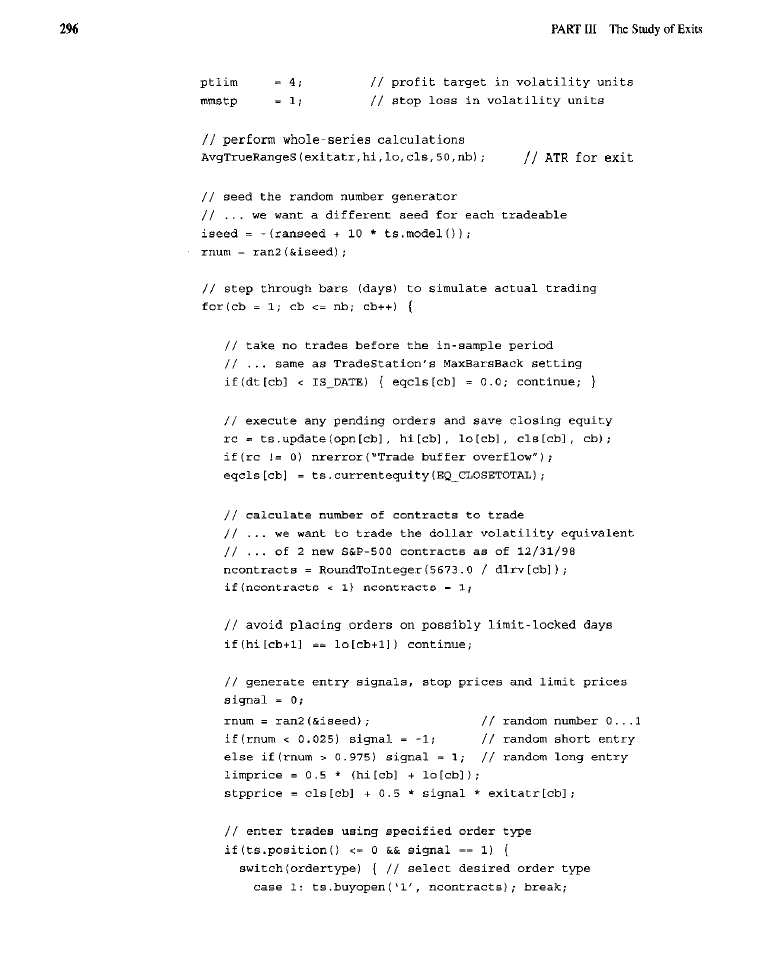

case 2:
*contracts,;
case 3:
break;
e l s e
s i g n a l = =
(
(
select desired order type
case 1:
break;
2 :
b r e a k ;
case 3:
default:
sell order selected”);
instruct simulator to employ standard exit
=
,
process next
The code is similar to that presented in earlier chapters. Only the generation
of the entry signals has changed. Entry signals are now issued using a pseudo-ran-
dom number generator (RNG). Before entering the loop that steps through bars to
simulate
process of trading, the RNG is initialized with a unique seed. The ini-
tialization seed is determined by the market number and by a parameter
By changing the parameter, a totally different sequence of random entries is gen-
erated. The exact seed values are irrelevant in that, for every seed, a unique series
will be generated because the period of the RNG is extremely large.
The RNG used is the one described as
in
Recipes in C
(Press
et al., 1992). The period of this RNG is greater than 2 multiplied by 10’“. This
RNG is by far better than those that normally come as part of a programming lan-
guage library. Inside the loop, where trading actually takes place, signals are gen-
erated based on random numbers. The steps are very simple. On each bar, a
uniformly distributed random number between 0 and 1 is obtained from the RNG.
If the random number is less than 0.025, a short signal is generated. The proba-
bility of a short being generated on any bar is 0.025; i.e., a short signal should
occur every 40 bars, on average. If the random number is greater than 0.975, a long
signal is issued, these signals should also occur, on average, every 40 bars. In other
words, on average, a long or a short trading signal should occur every 20 bars. The
limit and stop prices are calculated in the usual way. Orders are placed and exits
specified in the usual manner.
The steps that are used to conduct each of the three tests are as follows: On
the in-sample data and for each entry order type, 10 distinct series of random
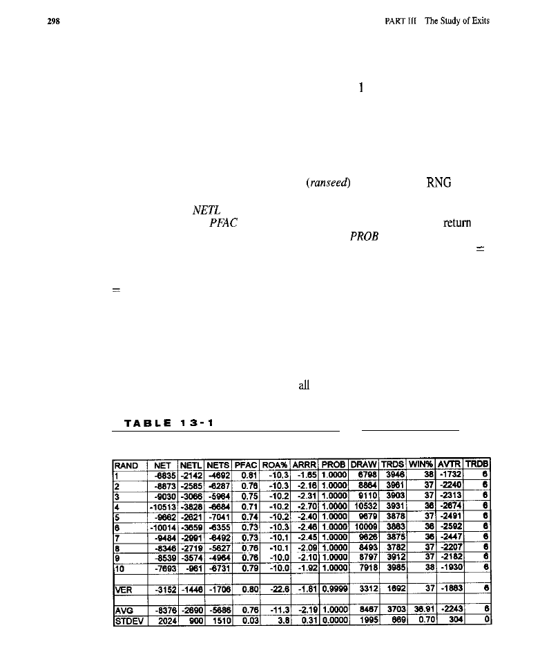
entries are generated and traded. The best of those sequences are then examined
on the verification or out-of-sample data. The process mimics that of optimizing a
parameter in a real system by stepping it from, e.g., to 10; here the parameter
simply selects a totally different series of random entries for each value.
Test Results
Tables 13-1, 13-2, and 13-3 present the portfolio performance that resulted from
trading random entries with the standard exit strategy. Each of the numbers in the
column RAND represents a seed modifier
that causes the
to gen-
erate a different sequence of random entries. NET = the total net profit, in thou-
sands of dollars.
= the total net profit for the longs. NETS = the total net
profit for the shorts,
= the profit factor. ROA% = the annualized
on
account. ARRR = the annualized risk-reward ratio.
= the statistical signif-
icance or probability, DRAW = the drawdown, in thousands of dollars. TRDS
the number of trades. WIN% = the percentage of wins. AVTR = the average trade,
in dollars. TRDB = the average bars per trade, rounded to the nearest integer. VER
the performance for the random sequence that provided the best in-sample per-
formance when this sequence is continued and then tested on the verification sam-
ple. AVG = the average in-sample value of the numbers in rows 1 through 10.
STDEV = the standard deviation for the in-sample performance data shown in
rows 1 through 10.
Test I: SES with Random Entries at the Open.
This system did not perform very
well in-sample. The average trade, over
10 randomizations, lost $2,243, with a
Results for the Standard Exit with Random Entries at the Open
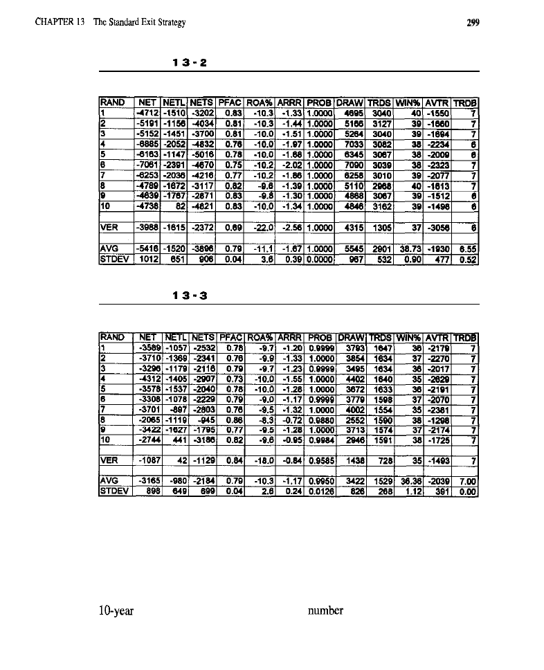
T A B L E
Results for the Standard Exit with Random Entries on a Limit
T A B L E
Results for the Standard Exit with Random Entries on a Stop
standard deviation of $304. In terms of average dollars-per-trade. the less attractive
systems that were tested when studying entries were on par with the results for the
current system. In fact, some of them performed significantly worse than chance.
The percentage of wins was very stable, with the average at 36.91% and a standard
deviation of only 0.7%. The total number of trades taken per commodity, over the
in-sample period, was 3,703, about the
it should be, given the prob-
ability of taking a random entry on any bar.
Out-of-sample, performance was within the expected range, consistent with
in-sample performance. The percentage of wins was
very close to that for
sample results. The average loss per trade was $1,883, which is within 1 standard
deviation of the in-sample estimate. Obviously, the standard exit was unable to
pull a profit out of trades entered randomly.
Test 2:
with Random Entries on Limit.
Table
is identical to Table 13-
1, except that it shows portfolio behavior for the standard exit with random entries
taken on a limit order. In-sample, the average loss per trade of $1,930 was some-
what less, demonstrating the effect of the limit order in reducing transaction costs.
The standard deviation was somewhat higher: $477. The percentage of winning
trades (38.73%) was just under 2% better, due to the better prices achieved with a
limit entry. As was anticipated, other than such small changes as those described,
nothing else in Table
is of any great interest.
Out-of-sample, the system lost $3,056 per trade, just over 2 standard deviations
worse than in-sample behavior. For whatever reason, the limit order may have had
some real effect with random entries, making the system perform more poorly in
recent
The percentage of wins was also slightly worse, i.e.,
just under 2
standard deviations below in-sample behavior, but on
with
at the open.
Test 3: SES with Random
on Stop.
Table 13-3 contains information
about the portfolio behavior for the standard exit when trades were entered ran-
domly on a stop. In terms of dollars-per-trade, in-sample performance was
between that of the other two orders, with a loss per trade of $2,039. The standard
deviation was $391. The percentage of wins was lower,
with a standard
deviation of 1.12%. The lower percentage of wins probably reflects the poorer
entry prices achieved using
stop.
Out-of-sample, the average trade and percentage of wins were within 2 Stan-
dard deviations plus or minus the in-sample figures, demonstrating that
sample performance was within the statistically expected range and fundamentally
no different from in-sample performance.
The performance figures in Tables 13-l through 13-3 provide a baseline (in
the form of means and standard deviations) that can serve as a yardstick when
evaluating
entries studied in Part of this book. For this purpose the $TRD
and WIN% figures are the best ones to use since they are not influenced by the
number of trades taken by a system.
Market-by-Market Performance for
with Random Entries at Open,
In
Table 13-4, the behavior of
standard exit with random entries taken at the open
is broken down by market and by sample. The particular randomization used was
the one that produced the best in-sample
(in terms of annualized
to-reward ratio) in Test 1. The leftmost column
contains the commodity
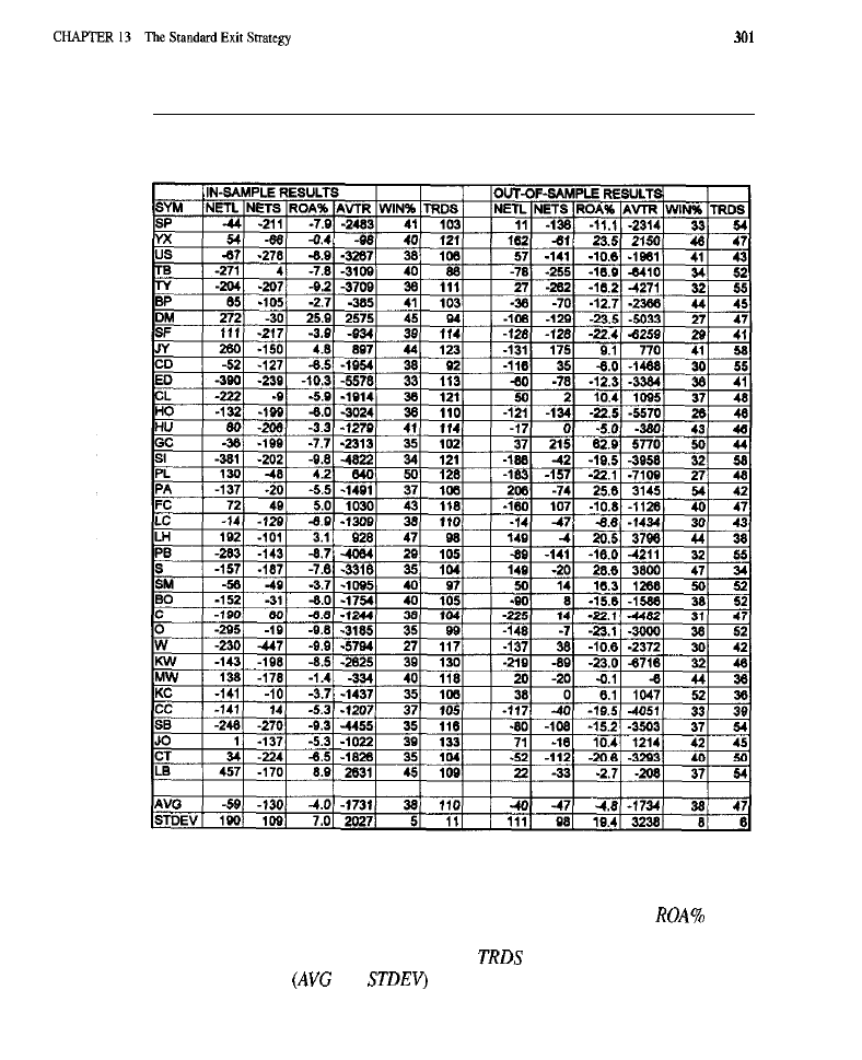
T A B L E 1 3 - 4
Market-by-Market Results for the Standard Exit with Random Entries
at the Open
symbol. The remaining columns contain information about various aspects of per-
formance, both in-sample and out-of-sample.
NETL
and
NETS are
the net profits
for long and short positions (respectively), in thousands of dollars.
=
the
annualized return-on-account.
AVTR
= the average dollars profit or loss per trade.
WIN%
= the percentage of winning trades.
= the
number of trades taken.
The last two rows
and
show the averages and standard deviations

(respectively) across all markets for the various performance figures.
In-sample, the British Pound, the Japanese Yen, Feeder Cattle, Live Hogs,
and Lumber were the only markets that bad positive returns. Only the
Deutschemark had a strong return on account at 25.9% annualized. Out-of-sam
ple, the NYFE, the Japanese Yen, Light Crude, COMEX Gold, Palladium, Live
Hogs, Soybeans, Soybean Meal, Coffee, and Orange Juice had positive returns.
Only the Japanese Yen and Live Hogs were profitable in both samples. The ran-
dom entry system was among the least consistent systems of those examined in the
study of entries.
The average trade, across all markets, lost $1,731 in-sample and $1,734
of-sample. Long trades lost less than shorts, a finding observed many times. In-
sample,
the currencies, except the Canadian Dollar and Eurodollars, were
profitable on the long side. These are trendy markets, and therefore, such prof-
itability is likely due to the behavior of the standard exit, not to chance factors
involved in the random entries.
The analysis of the standard exit with random entries taken using various
entry orders should serve well as a baseline of comparison for both the real,
random entries (studied in earlier chapters) and the more sophisticated exits (to be
studied in subsequent chapters).
TESTS OF THE MODIFIED SES
The next test involves changing the SES a bit, thus producing the
stan-
dard exit strategy
(MSES). The SES is made more realistic by allowing the money
management stop and profit target limit to function inside the bar, not merely at
the close. To avoid ambiguities in the simulation when using end-of-day data, all
entries are now restricted to the open. This allows complete freedom to explore a
wide range of exit strategies. Other than lifting the restriction to the close, the
MSES is identical to the original SES used when testing entries. The rules for the
MSES are as follows: Upon entry, set up an exit stop below (long positions) or
above (short positions) the entry price and an exit limit above (long) or below
(short) the entry price. Place the exit stop some multiple (the money management
stop parameter) of the average true range away from the entry price. Place the exit
limit some other multiple (the profit target parameter) of the average true range
away from the entry price. Exit on the close after 10 days have elapsed if neither
the money management stop nor the
target limit has yet closed out the trade.
A
average true range is used in these rules. The code below implements
random entries at the open together with the modified standard exit strategy.

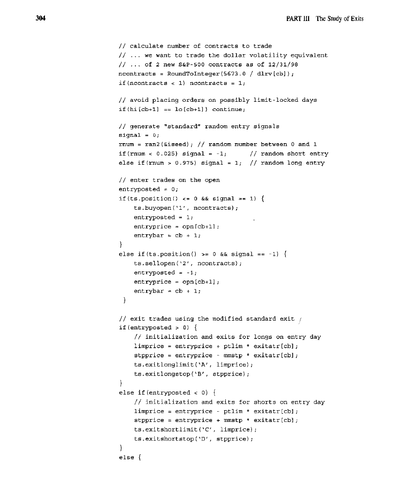

The code used to run the current test is identical to the code used for the ear-
lier test, except for changes required by the modified exit strategy. A trade is
entered on a random signal that is generated as discussed earlier. However, buying
and selling occur only on the open. In addition, information is recorded about
entry activity, i.e., whether an entry (long, short, or none) was posted on the cur-
rent bar
the price
at which the entry took place (if one
was posted), and the bar on which it took place
This data is required in
computing the exits. The exits are then generated. If an entry is posted for the next
bar (i.e., if the market is entered long or short at the open of the next bar), a prof-
it target and a stop loss are also posted for that bar. For the longs, the stop loss, or
money management stop, is set at the entry price minus a parameter that is
by the average true range. The limit price for the profit target is set as the
entry price plus another parameter that is multiplied by the average true range. If,
on the current bar, a short entry is posted for the next open, then orders are also
posted to exit the resulting short position on a limit or a stop. The limit and stop
are calculated in a manner similar to that for the longs, except the directions are
flipped around. If a given bar is not an entry bar, a check is made to determine
whether there is an existing position after the close of the bar. If there is, two
orders (possibly three) are posted: the money management stop and profit target
limit orders, using the stop and limit prices calculated on the bar the entry was ini-
tially posted; and if the trade has been held for more than
bars, an order
to exit on the close is also posted.
TEST RESULTS
Test 4:
MSES with Random Entries at Open.
Table 13-5, which has the same
format as Tables 13-l through 13-3, provides data on the portfolio performance of
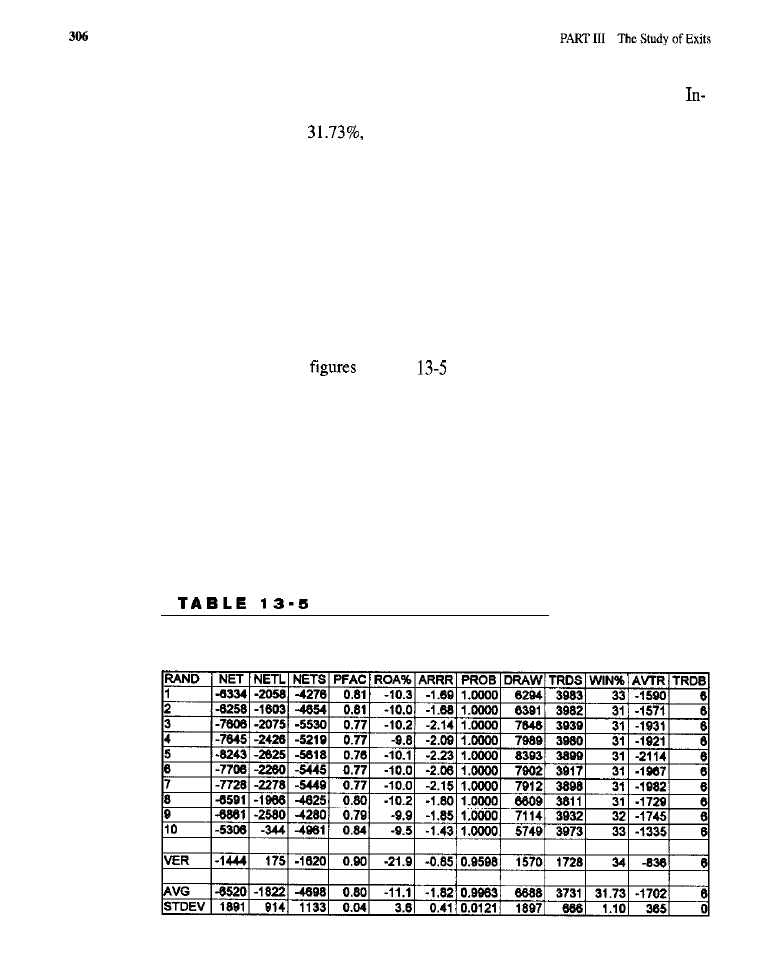
the modified standard exit strategy with trades entered randomly at the open,
sample, the average trade. lost $1,702, with a standard deviation of $365. The per-
centage of wins was
with a standard deviation of 1.10%. The average
trade lost less than it did in the tests of the original, unmodified SES. The reduc-
tion in the loss on the average trade was undoubtedly caused by the ability of the
MSES to more quickly escape from bad trades, cutting losses short. The more
rapid and frequent escapes also explain the decline in the percentage of winning
trades. There were fewer wins, but the average loss per trade was smaller, an inter-
esting combination. Overall, the MSES should be regarded as an improvement on
the unmodified standard exit.
Out-of-sample, the average trade lost $836. Statistically, this was signifi-
cantly better than the in-sample performance. It seems that, in more recent years,
this exit provided a greater improvement than it did in earlier years. The markets
may be more demanding than they were in the past of the ability to close out bad
trades quickly. Other
in Table
indicate a similar pattern of changes.
Market-by-Market Results
for
MSES with Random Entries at Open. Table 13-
6 contains the market-by-market results for the MSES with the best set of random
entries taken at the open. The
best
set was chosen from the randomizations shown
in Table 13-5. The Swiss Franc, Light Crude, Heating Oil, COMEX Gold, and
Live Cattle had positive returns both in- and out-of-sample. For some markets, the
MSES was able to pull consistent profits out of randomly entered trades! Many
more markets were profitable in both samples than when the unmodified SES was
Results for the Modified Standard Exit with Random Entries
at the Open
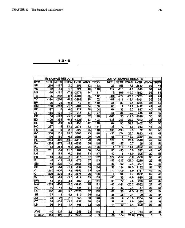
used, again a sure sign that the more responsive, modified exit is better. As usual,
and across both samples, the long side was more profitable (lost less) than the
short side. Surprisingly, out-of-sample, the long side actually turned a very small
whole-portfolio profit with this exit strategy; it is, however, nothing one would
want to trade.
T A B L E
Market-by-Market Results for the Modified Standard Exit
with Random Entries at the Open

CONCLUSION
The results clearly demonstrate that many of the entry strategies tested in earlier
chapters using the SES were no better than random entries. Sometimes they were
worse. The results also indicate that the
is not a great exit strategy. The
MSES, which simply lifts the restriction of the exit to the close, performed much
better and even managed to pull a small profit out-of-sample on the long side. The
MSES should still be considered a minimalist exit strategy, but the results support
the contention that a really good exit strategy is, more than anything else, the key
to successful trading. If the findings from this and previous studies are correct, it
should be possible to find an exit strategy that can actually extract substantial prof-
its from randomly entered trades, at least in some markets. Such an exit strategy
would substantiate what many great traders have said: An experienced trader,
skilled in money management, can make a profit even with a bad system, while a
novice trader, unskilled in money management, can lose everything trading a great
system
in this context, usually referring to an entry model). In all the
remaining tests in
book, the MSES will replace the original, unmodified exit
strategy (SES).
WHAT HAVE WE LEARNED?
. A good exit strategy is extremely important. It can even pull profits from
randomly entered trades! Think of what it could do for trades entered on
the basis of something better than the toss of the die.
. Even simple modifications can make a big difference, as evidenced by the
results above where slight changes proved effective.
. When combined with the suboptimal SES, many of
entry strategies
tested in the previous section of this book can be seen to perform no bet-
ter than the random one. Some even did worse! Of course, a few per-
formed dramatically better than did the random entry model.

C H A P T E R 1 4
Improvements on the Standard
Exit
continuation of the endeavor to improve upon the standard exit strategy
and develop a good exit, a number of modifications are explored. In the previous
chapter, it was demonstrated that the exit strategy can have a substantial impact on
the overall performance of a trading system. To make it more compatible with the
kinds of exit strategies examined in this and the next chapter, the original SES
(used in the study of entries) was changed and became the modified SES (or
MSES): While maintaining consistency, the restriction of exiting at the close was
removed. It was no longer necessary to restrict the exit to the close, because in the
study of exits, entries are restricted to the open. In previous chapters, entries were
not restricted to the open. Therefore, to avoid ambiguity in the simulations, it was
necessary to restrict exits to the close. The MSES represents a kind of baseline,
minimalist exit that can serve as a standard for comparing better exit methods, as
well as provide some consistency and comparability with the unmodified SES. In
this chapter, variations, both small and large, of the MSES are explored in an
attempt to
a better exit strategy.
PURPOSE OF THE TESTS
When specifying the original SES (as well as when modifying it so that
bar stops and limits could be used), specifications for the tightness of the money
management stop and closeness of the profit target were arbitrary and fixed. For
long entries, the money management stop was placed at 1 average true range unit
below the entry price, while the profit target was placed 4 average true range units
above the entry price. For short entries, the placements were reversed. The inten-
tion was to place a stop fairly close in so that losing trades would quickly be taken

3 1 0
out, while placing the profit target far enough away so profits would not be cut
short on trades that were favorable. The first test below examines the performance
of the stop and profit target when the arbitrary settings are adjusted.
The second set of tests involves replacing the
money management stop
in the MSES with a more dynamic stop. The minimalist MSES lacks many
able characteristics. One of the features any good trader wants in an exit is the abil-
ity to lock in at least some of the paper profit that develops in the course of a
successful trade, i.e., to avoid having to watch profitable trades turn into losers.
Locking in some of the profit can be accomplished using a trailing stop: Instead
of having a money management stop placed a fixed distance from the entry price,
the stop moves toward current prices as the trade becomes profitable. As prices
move in the trade’s favor, the stop moves in along with them, locking in a propor-
tion of the developing profits. Should the market reverse, the trade will not be
closed out at a loss, as might have been the case with the
stop, but at a prof-
it, if the moving stop has gone into positive territory. There are several strategies
for the placement and relocation of a stop designed to prevent winning trades from
turning into losers and to lock in as much of the unrealized profit as possible. The
second set of tests explores such strategies.
Originally, the profit target in the MSES (and SES) was implemented as a
limit order with a
placement. In the third set of tests, the fixed
target
is, like the stop in the previous tests, replaced with something more dynamic. It
would be desirable if the profit target could also move in toward the prices, espe-
cially in languishing trades. This would enable the trader to exit at a better price,
perhaps even with a small profit, in the absence of strong, favorable movement.
Exiting the market on spikes or noise should lead to more profitable trades than
simply exiting on a time constraint or waiting for the money management stop to
be hit. At the same time, the trader does not want the profit target to cut profits
short. A
target that is too close might provide a higher percentage of win-
ning trades, but it will also significantly limit the size of the profits. In all likeli-
hood, it will cause the overall strategy to perform less well. It should be
advantageous to make the profit target dynamic in the same way that the stop was
made dynamic, i.e., to place the profit target far away from the market at the begin-
ning of the trade, or when the market is steadily moving in a favorable direction,
In this way, it would not be necessary to settle for a small
on a potentially
very profitable trade; the trader could “let profits run.” Conversely, in trades that
are languishing, or when the market is exhibiting blow-off behavior, the profit tar-
get could be made to move in tight to close out the trade, and to do so at the best
possible price, before the market has a chance to reverse. Modifications of the
profit target limit order placement are studied below.
Finally, the time limit exit from the MSES model is adjusted and tested on
the assumption
effective dynamic stops and profit targets, a short time
limit is no longer so necessary. Trades will be exited quickly by other means if

they are languishing, but will be held for as long as possible if favorable move-
ment is occurring. The intention is to let profits develop and not be cut short sim-
ply because of an order to exit on an arbitrary time limit.
TESTS OF THE FIXED STOP AND
PROFIT TARGET
The MSES makes use of a fixed stop and profit target that do not change their place-
ments during a trade. Originally, the parameters for the placement of these stops
were somewhat
and certainly not optimal. What happens when these para-
meters are stepped through a range of values in search of an optimal combination?
In this test, the money management stop parameter is stepped from 0.5 to 3.5
in increments of 0.5. The profit target limit parameter is also stepped from 0.5 to
5 in increments of 0.5. The profit target parameter is simply the multiple of the
average true range used in placing the profit target limit. Likewise, the money
management stop parameter is the multiple of the average
range used for plac-
ing the money management stop.
float
float
float
float
float
l eqcls)
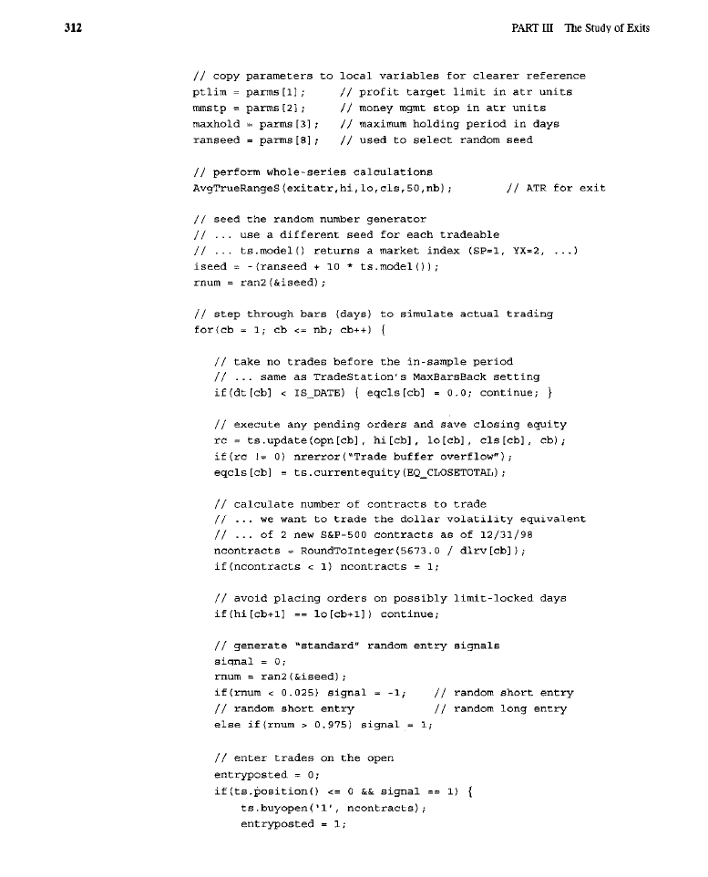

313
The code implements the standard random entry at the open and the modi-
fied standard exit strategy. The rules for the exit are as follows: A limit order exit
is placed a certain number of true range units above (long) or below (short) the
entry price. The number of
range units that the limit order is placed away from

the entry price is specified by the parameter
Besides the
target limit,
an exit stop is placed a specified number of average true range units below (long)
or above (short) the entry price. The parameter
determines the number of
true range units that the stop is placed away from the entry price. Finally,
is a
parameter
that specifies the maximum time any position is
not closed out
by the profit target limit or money management stop, all
trades will be closed out with an exit at the close after
days or bars have
elapsed since entry. In the test,
is fixed at a value of 10, the same value
used throughout the tests in this book.
Table 14-l shows the annualized risk-to-reward ratio (ARRR), the percent-
age of winning trades (WIN%), and the average trade profit or loss
for
every combination of money management stop and profit target limit parameter
settings. At the right of the table, the AVG or average values (average taken over
all money management stop parameters) for all the performance figures are pre-
sented for each profit target limit parameter value. At the bottom of the table,
the AVG or averages (taken over all profit target limit parameters) for each of the
money management stops are shown.
A number of things are immediately apparent in the results. As the profit tar-
get limit got tighter, the percentage of winning trades increased; this was expected.
A tight profit target has a greater chance of being hit and of pulling a small profit
out of the market. However, the increased percentage of winning trades with
tighter profit targets was not sufficient to overcome the effects of cutting profits
short on trades that had the potential to yield greater profits. Looser profit targets
performed better than tight ones. For most of the profit target limits, there was an
optimal placement for the money management stop, between a value of 1.0 and
2.0 average true range units away from the entry price. As the stop got looser, the
percentage of winning trades increased, but the other performance figures wors-
ened. As it got tighter, the percentage of winning trades declined along with the
other measures of performance.
The overall optimal performance, in terms of both annualized risk-to-reward
ratio and average trade, was with a profit target limit of 4.5 and a money manage-
ment stop of 1.5. As deviation from the optimal combination occurred, the annu-
alized risk-to-reward ratio increased, as did the average loss per trade. There was
relatively little interaction between placement of the profit target and the money
management stop. The values that were optimal for one varied only slightly as the
parameter controlling the other was adjusted. Another almost equally good com-
bination of parameters was 1.5 and 4 (profit target and stop, respectively). This
provided a very slightly better average trade and a trivially worse annualized
to-reward ratio. It is interesting that the arbitrarily assigned values came fairly
close to the optimal values, appearing only one cell away from the optimal cells in
Table 14-l. The optimal values, however, provided 6% more winning trades than
the arbitrary
of 4 (profit target) and 1 (stop).
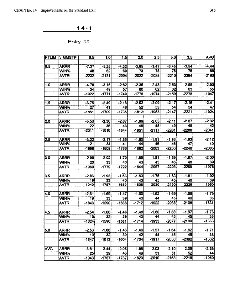
T A B L E
In-Sample Portfolio Performance with Modified Standard Exit and
Random
a Function of Profit Target Limit (Left) and Money
Management Stop (Top) Parameters

The percentage of wins for the optimal solution was 39%. When the num-
bers were examined in relationship to those for a profit target limit of 0.5 (with the
same stop), 69% (instead of 39%) winning trades resulted, but with a much worse
risk-to-reward ratio and average trade. This clearly shows the importance of let-
ting profits run or, at least, not cutting them short.
No combinations of parameters yielded profitable results. Given
this is
a minimalist exit strategy, and that random entries were being used, such an out-
come was expected. Nevertheless, the performance of the exit strategy across dif-
ferent parameter combinations can be compared.
Conclusion
Profits should not be cut short even though a higher percentage of winning trades
might be gained. Doing so may make the average trade a larger loser or smaller
winner. In addition, there appears to be an optima1 placement for a fixed money
management stop. Too wide a stop increases the percentage of wins. However, it
also increases the overall loss. Too tight a stop keeps the individual losses small,
but drastically cuts the percentage of winning trades, again resulting in worse
overall performance. An optimal value provides a moderate percentage of winning
trades and the best performance. In this case, the optimal distance to place the
money management stop away from the entry price was 1.5 average true range
units. With some entry systems, the optima1 placement might be much closer.
TESTS OF DYNAMIC STOPS
In this group of tests, the
money management stop of the MSES is replaced
with what will; it is hoped, be a much better stop. The placement of the stop is
dynamically adjusted. The goal is to capture as much unrealized profit as possible,
while not turning potentially profitable trades into losing ones, as might happen
with an overly tight, fixed stop.
There are many ways to adjust the stop so that it follows or trails the market,
locking in some of the profit that develops in the course of a trade. One popular
method is, for long positions, to place the stop for the next bar at the lowest of the
lows of the current and previous bars. The stop is only placed at progressively
higher levels, never lower levels. For short positions, the stop is placed at the high-
est of the current bar’s and previous bar’s highs, It is only allowed to move down,
never up. This simple methodology is examined in the first test.
The second test is of a dynamic stop that mimics the fixed stop used in the
MSES. The stop is adjusted up (long) or down (short) based on the current price
minus (long) or plus (short) a multiple of the average true range. Unlike the stop
used in the MSES, where the placement was fixed, the placement revisions of
this stop are based on current market value. The revised placements may only

occur in one direction: up for long positions, down for short ones. The intention
is to keep the stop a similar statistical distance from the best current price
achieved at each stage of the trade, just as it was from the original entry price.
The stop for long positions is calculated as follows: (1) Subtract from the entry
price a parameter
multiplied by the average
range (the result is the
stop for the next bar). (2) On the next bar, subtract from the current price anoth-
er parameter
multiplied by the average true range. (3) If the stop resulting
from the calculations in Step 2 is greater than the current stop, then replace the
current stop with the resultant stop: otherwise the stop remains unchanged. (4)
Repeat Steps 2 and 3 for each successive bar. In the stop for short positions, the
multiples of the average true range are added to the market prices and the stops
are ratcheted down.
The third test involves a more sophisticated approach. For long positions, the
stop is initialized a certain number of average true range units below the entry
price, as usual. The stop is then moved up an amount that is determined by how
far the current prices are above the stop’s current value. For short positions, the ini-
tialization occurs above the entry price, and the stop is moved down to an extent
determined by how far the current prices are below it. The stop initially moves in
quickly, losing
as it reaches the vicinity of the current price level. This
method involves nothing more than a kind of offset exponential moving average
except that the moving average is initialized in a special way on entry to
the trade and is only allowed to move in one direction; i.e., the stop is never polled
further away from the market, only closer. The stop for long positions is calculat-
ed as follows: (1) Initialize the stop to be used on the entry bar by subtracting from
the entry price a parameter
multiplied by the average true range. (2) At
the next bar, subtract from the high a parameter
multiplied by the average
true range; then subtract the current placement of the stop, and finally multiply by
another parameter
(3) If the resultant number from Step 2 is greater than
zero, then add that number to the value of the current stop; otherwise the stop
remains unaltered. (4) Repeat Steps 2 and 3 for each successive bar. In the stop for
short positions, the multiples of the average
range are added to the market
prices and only corrections that are negative are added to the stop prices.
static void Model
float
float
float
*hi.
float l cls, float *vol. float
float
random entry tests of the standard exit
strategy modified to use “dynamic”
parameters
vector
of
in
form
vector
opening prices

3 1 8
v e c t o r
o f h i g h
prices
of low prices
vector
prices
vector
of open interest numbers
vector
of average dollar
of bars in data series or
trading simulator
instance
vector
closing equity levels
declare local scratch variables
static
*contracts,
signal,
static float
ptlim,
limprice,
static
static float
static long
copy parameters to
used to set the initial stop
additional stop parameter
additional stop parameter
ptlim
profit target limit in
units
type of
dynamic
stop to
maximum holding period in days
=
to
perform
calculations
for exit
number generator
use a different seed for each
returns a market index
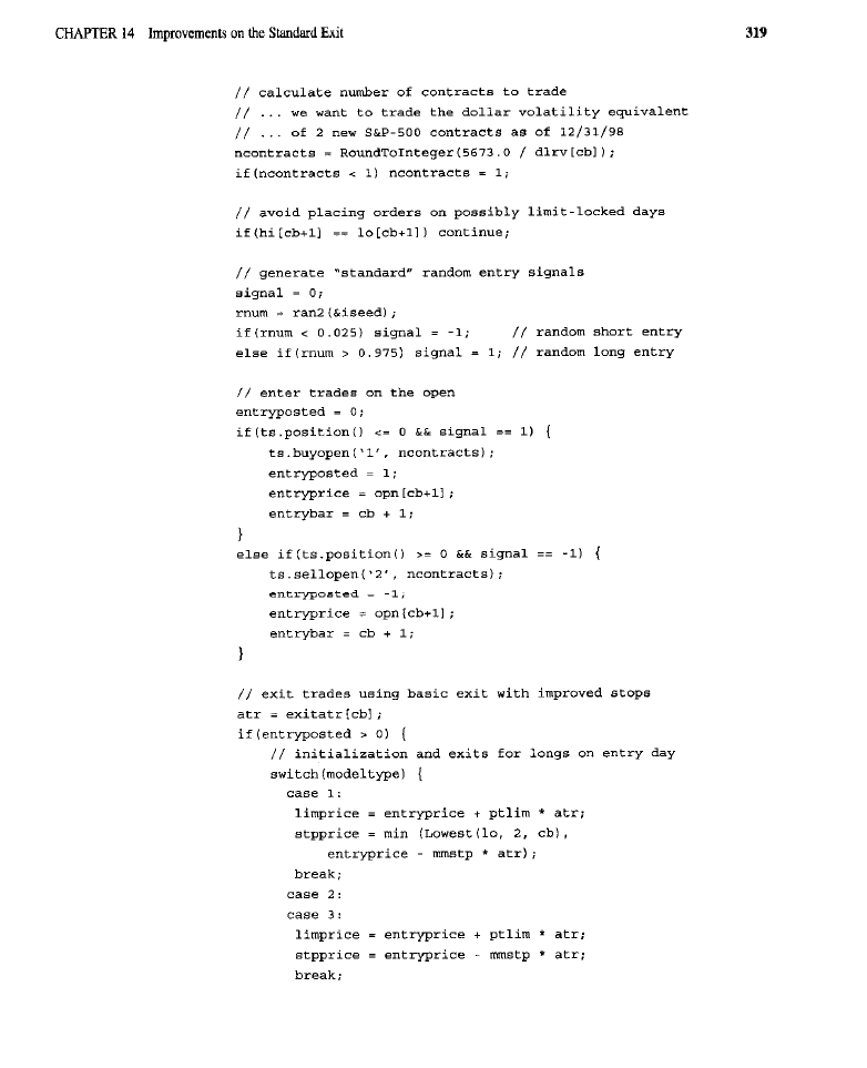
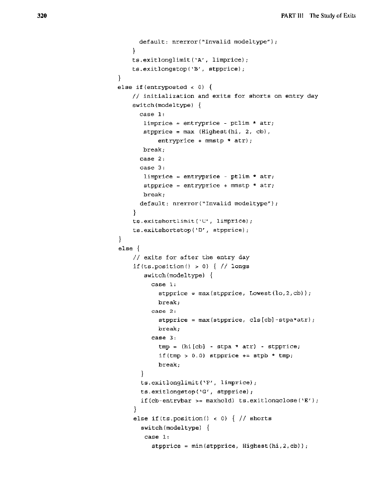

l
stpprice;
,
process next
The code above implements the MSES with the original
stop replaced
with one of the three more responsive, dynamic stops, The parameter
selects the stop, and depending on which is to be tested, up to three other con-
trolling parameters are set and adjusted. For the two-bar highest-high/lowest-
low (HHLL) stop, the parameter (mmsrp) is the multiple of the average true
range that is added to or subtracted from the entry price to obtain the stop price
for the entry bar. The stop price on the entry bar is set to either the lowest low
of the last two bars or the entry price plus or minus the specified multiple of the
average true range, whichever is further away from the current market price. For
the other two kinds of stops (ATR-based and
the stop price on the entry
bar is initialized to the usual value, i.e., the entry price minus (long) or plus
(short) the money management stop parameter
multiplied by the aver-
age true range.
On each bar after the entry bar, the stop price is adjusted. The adjustment
used depends on the particular type of stop being employed, as selected by the
parameter. For the HHLL stop, the highest high or lowest low is cal-
culated according to whether the position is short or long (respectively). If the
result of the calculation is closer to the current market price than the current stop
price is, then the current stop price is replaced with the new value. For the next
model (dynamic ATR-based stop), a second money management stop parameter
is multiplied by the average true range. Then the resultant number is sub-
tracted from (long) or added to (short) the current closing price. If the resultant
number is closer to the market than the current value of the stop price, the stop
price is replaced with that number and, therefore, moved in closer to the market.
For the third type of stop
a stop parameter
is multiplied by the
average true range, and then subtracted from the current high (longs) or added to
the current low (shorts) as a kind of offset. The stop price is then subtracted from

the resultant number. The result of this last calculation is placed in a variable
The stop price is updated on successive bars by adding
multiplied by
another parameter
a correction rate coefficient) to the existing stop price.
The current stop price is adjusted, however, only if the adjustment will move the
stop closer to the current price level. The computations are identical to those used
when calculating an exponential moving average
The only difference is
that, in a standard exponential moving average, the stop price would be correct-
ed regardless of whether the correction was up or down and there would be no
offset involved. In this model,
determines the effective length of an expo-
nential moving average that can only move in one direction, in toward the prices.
Test of Highest-High/Lowest-Low Stop
In this test
=
initial money management stop parameter con-
trols the maximum degree of the stop’s tightness on the first bar. It is stepped from
0.5 to 3.5 in increments of 0.5.
Each row in Table 14-2 presents data on the in-sample performance of each
of the values through which the parameter was stepped
The last row
describes the behavior of the model with the best parameter value (as found in the
stepping process) retested on the out-of-sample data. Table 14-2 may be interpret-
ed in the same way as the other optimization tables presented in this book, in the
table,
DRAW
represents drawdown, in thousands of dollars.
This stop appears to have been consistently too tight, as evidenced by a decreased
percentage of winning trades when compared with the baseline
model. In the
previous test, the best solution
parameter 1.5,
parameter 4.5) had 39%
wins, had a risk-to-reward ratio of 1.46, and lost an average of $1,581 per trade. In
the current test, the best solution has only 28% of
trades winning in-sample and
29% out-of-sample. Many potentially profitable trades (some of the trades that would
have been profitable with the basic MSES, using an optimal fixed stop) were convert-
ed to small losses. The tightness of this stop is also demonstrated by the total number
of bats the average trade was held
compared with the usual 6 to 8 bars. The aver-
age risk-to-reward ratio (-2.52 in-sample and -2.38 out-of-sample) and the average
loss per trade ($1,864 in-sample, $1,818 out-of-sample) have also significantly wors-
ened when compared
the optimal fixed stop. The
stop is obviously
no great shakes, and one would be better served using a fixed, optimally placed stop,
like that which forms part of the MSES when used with optimized
such
as those discovered and shown in the test results in Table 14-1.
Test of the Dynamic ATR-Based Stop
In this model, the two parameters (represented in the code as
and
are
multipliers for the average
range. They are used when calculating placement of
the stop on the entry bar and later bars, respectively. The entry bar stop parameter
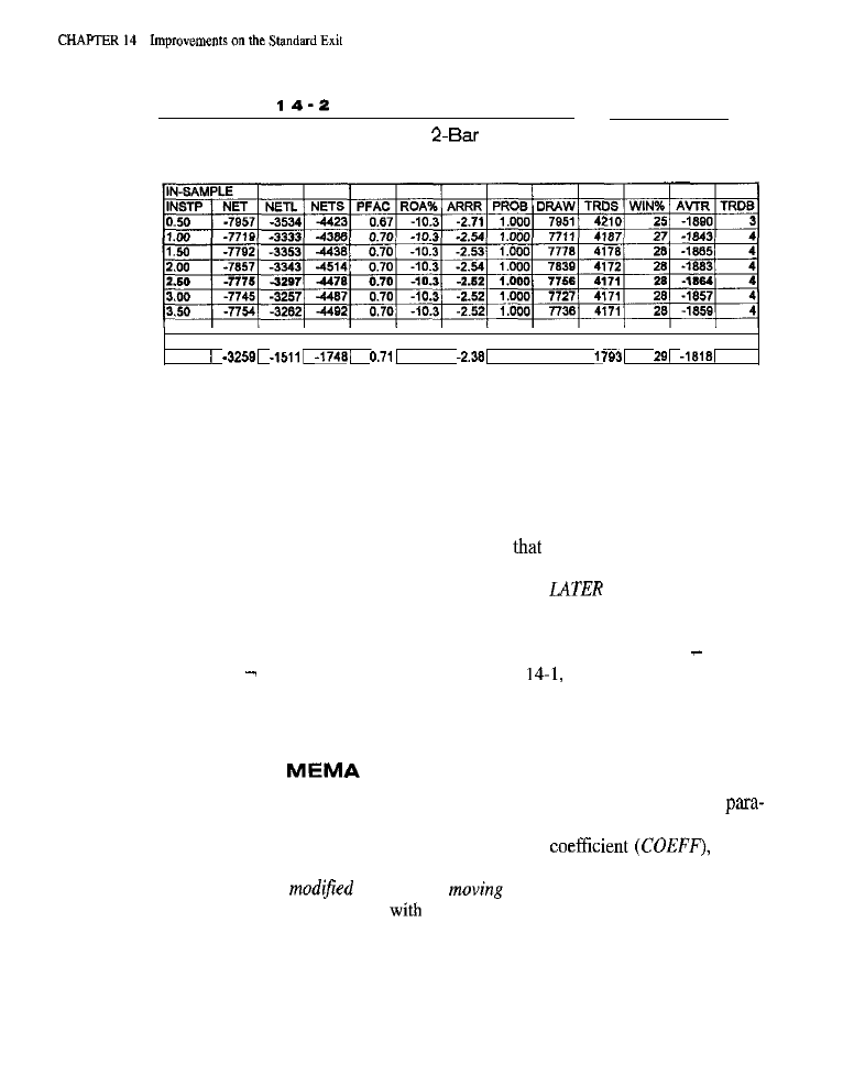
323
T A B L E
Portfolio Performance for the
Highest-High/Lowest-Low Trailing
Stop with the Optimal Fixed Profit Target Found in Table 14-l
OUT-OF-SAMPLE
I
I
I
I
I
I
I
I
2.50
-22.41
1.000~
34501
4
(FIRST
in Table 14-3) and the parameter for the stop after the entry bar
(LATER) are
both stepped from 0.5 to 3.5 in increments of 0.5.
As with the previous tests of stops, the parameters had a gradual effect on
performance and did not interact with one another to any great extent. An exami-
nation of the average performance for each value of the entry bar stop parameter
reveals that the best results, in terms of risk-to-reward ratio, were obtained when
that parameter was set to 2. For the parameter
applied to later bars, the best
average result was achieved with values of either 2 or 2.5. For individual combi-
nations of parameters,
a FIRST
parameter of
2
and a
parameter of 2.5 pro-
duced the best overall performance, with the least bad risk-to-reward ratio and
nearly the smallest loss per trade. This stop model was marginally better than the
optimal fixed stop, used as a baseline, that had a risk-to-reward ratio of 1.46, as
opposed to 1.40 in the current case. As in Table
the best solution is shown
in boldface type. The percentage of winning trades (42%) was also marginally bet-
ter than that for the optimal fixed stop (39%).
Test of the
Dynamic Stop
There are three parameters in this model: the initial money management stop
meter, which sets the stop for the first bar; the ATR offset parameter
(ATRO
in
Table 14-4); and the correction or adaptation rate
which
determines the relative rate at which the stop pulls in to the market or, equivalently,
the speed of the
exponential
average underlying this model. All
three parameters are optimized
an extensive search.
Table 14-4 shows portfolio performance only as a function of the ATR offset
and the adaptation rate coefficient, the most important parameters of the model.
The initial stop parameter was fixed at 2.5, which was the parameter value of the
optimal solution.
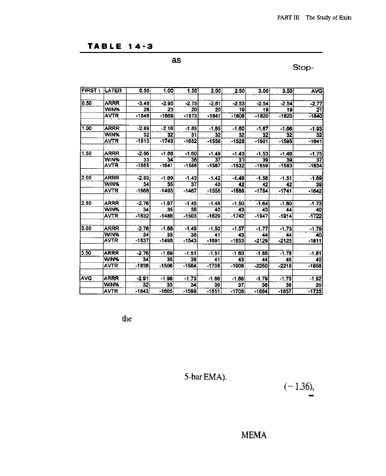
32.4
Portfolio Performance
a Function of First-Bar and Later-
Bar Stop Parameters Using the Dynamic ATR-Based
Loss Model
Again,
model responded in a well-behaved manner to changes in the para-
meter values. There was some interaction between parameter values. This was
expected because the faster the moving average (or adaptation rate), the greater the
average true range offset must be to keep the stop a reasonable distance from the
prices and achieve good performance. The best overall portfolio performance (the
boldfaced results in Table 14-4) occurred with an ATR offset of 1 and an adaptation
rate coefficient of 0.3 (about a
Finally, here is a stop that performed
better than those tested previously. The risk-to-reward ratio rose
as did the
percentage of winning trades (37%) and the average trade in dollars ( $1,407).
TEST OF THE PROFIT TARGET
This test is the best stop thus far produced: The
stop had an initial money
management parameter of 2.5, an average true range offset of 1, and an adaptation
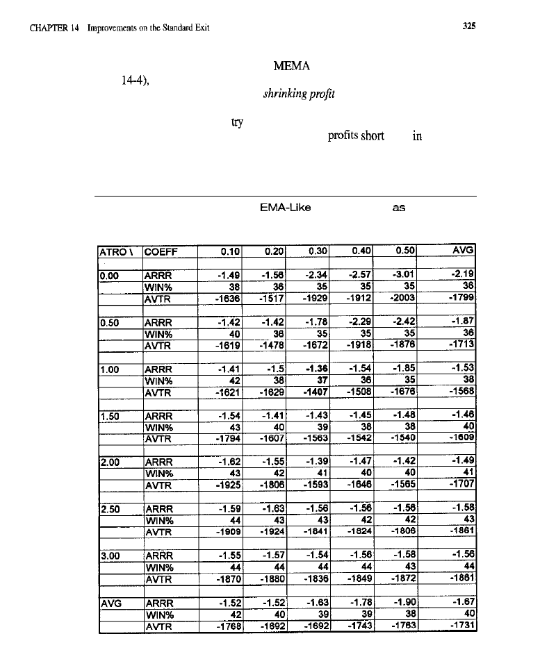
rate coefficient of 0.30. In the original
test above (the results reported in
Table
the optimal fixed profit target was used. In the current test, the optimal
fixed profit target is replaced with a
target, i.e., one that starts out
far away from the market and then pulls in toward the market, becoming tighter
over time. The intention is to to pull profit out of languishing trades by exiting
with a limit order on market noise, while not cutting
early the course
of favorably disposed trades. The approach used when constructing the shrinking
T A B L E 1 4 - 4
Portfolio Performance of the
Dynamic Stop
a Function
of the ATR Offset and Adaptation Rate Coefficient with an Initial Stop
Parameter of 2.5 ATR Units

profit target is very similar to the one used when constructing the
stop. An
exponential moving average is initialized in an unusual way; i.e., the running sum
is set to the entry price plus (long) or minus (short) some multiple
of the
average true range. In this way, the
target limit begins just as the fixed profit
target limit began. After the first bar, the price at which the limit is set is adjusted
in exactly the same way that an exponential moving average is adjusted as
bars
arrive: The distance between the current limit price and the current close is multi-
plied by a parameter
The resultant number is then subtracted from the cur-
rent limit price to give the new limit price, pulling the limit price in tighter to the
current close. In contrast to the case with the stop, the limit price is allowed to move
in either direction, although it is unlikely to do so because the limit order will
the trade out whenever prices move to the other side of its current placement. The
second parameter
controls the speed of the moving average, i.e., the shrink
age rate. The rules are identical to those in the test of the
stop above, except
as they relate to the profit target limit on bars after the first bar.
l
stpprice
case 2:
case 3:
4:
stpprice =

3 2 7
stpprice
2,
case 2:
3:
case 4:
l
stpprice
break;
stpprice);
stpprice
break;
2:
break;
3:
stpprice;
stpprice
l
case 4:
0.0) stpprice
break;
stpprice);
else
(
shorts
(
case 1:
stpprice
break;
2:
stpprice

s t p p r i c e ) ;
The code fragment above shows the implementation of the shrinking limit,
along with the
stop reported in Table 14-4.
Table 14-5 provides information on the portfolio performance as the initial
profit target limit
in the code,
in the table) and the shrinkage coeffi-
cient
in the code,
in the table) are varied. The parameter that con-
trolled the initial placement of the profit target, in average
range units away
from the price, was stepped from 2 to 6 in increments of 0.5. The shrinkage coef-
ficient was stepped from 0.05 to 0.4 in increments of 0.05. The best combination
of parameters produced a solution that was an improvement over the
target limit. The risk-to-reward ratio became
1.32, the percentage of winning
trades remained the same at
but the average loss per trades was less at
$1,325. Again, the model was well behaved with respect to variations in the para-
meters. The results indicate that care has to be taken with profit targets: They tend
to prematurely close trades that have large profit potential. As can be seen in Table
14-5, as the initial profit
placement became tighter and tighter, the percent-
age of winning trades dramatically increased, as more and more trades hit the prof-
it target and were closed out with a small profit. On the down side, the
risk-to-reward ratio and the average worsened, demonstrating that the increased
percentage of winning trades could not compensate for the curtailment of profits
that resulted from the tight profit target. Sometimes it is better to have no profit
target at all than to have an excessively tight one. The same was
for the shrink-
age rate. Profit targets that too quickly moved into the market tended to close
trades early, thereby cutting profits short.
TEST OF THE EXTENDED TIME LIMIT
In all the tests conducted so far, a position was held for only a maximum of
days. Any position that still existed-that had not previously been closed out by
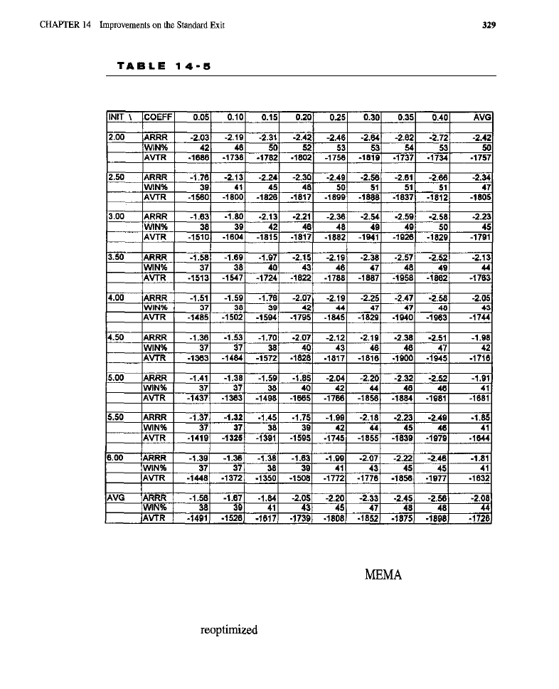
Portfolio Performance as a Function of the initial Profit Target Limit
Placement and the Shrinkage Coefficient
the stop or profit target-was closed out after 10 days, regardless of its profitabil-
ity. In this test, an exit strategy that uses an adaptive
stop, with optimal
parameters and a shrinking profit target, is examined. The only difference between
the test reported in Table 14-6 and the one reported in Table 14-5 is in the exten-
sion of the maximum time a trade may be held, from 10 to 30 days. The initial
profit target limit is
by stepping it from 5 to 7 in increments of 0.5.
Likewise, the shrinkage rate coefficient is stepped from 0.05 to 0.4 in increments
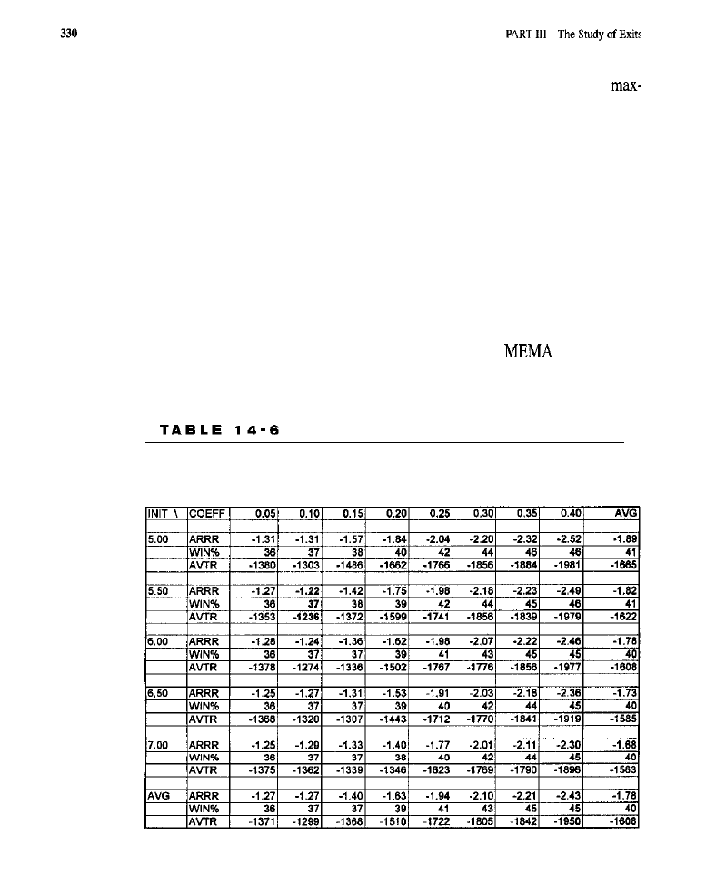
of 0.05. The code is the same as for the previous test. Only the setting of the
hold parameter, which controls the maximum time a trade may be held, is
changed.
The best performance was achieved with an initial target parameter of 5.5
and a shrinkage coefficient of 0.1. The average risk-to-reward ratio went from
1.32 to 1.22. The percentage of wins remained the same, but the average trade
lost only $1,236, rather than $1,325 in the previous test. Extension of the time
limit improved results, but not dramatically. Most trades were closed out well
before the time limit expired; i.e., the average trade only lasted between 6 and 10
bars (days).
MARKET-BY-MARKET RESULTS FOR THE BEST
EXIT
Table 14-7 reports on performance broken down by market for the best exit strat-
egy discovered in these tests, i.e., the one that used the
stop and the
shrinking profit target and in which the time limit was extended to 30 days. Both
in- and out-of-sample results are presented, and consistency between the two can
P o r t f o l i o P e r f o r m a n c e a s a F u n c t i o n o f t h e I n i t i a l P r o f i t T a r g e t L i m i t
S e t t i n g a n d t h e S h r i n k a g e C o e f f i c i e n t W h e n t h e T r a d e L i m i t I s
I n c r e a s e d t o 3 0 D a y s
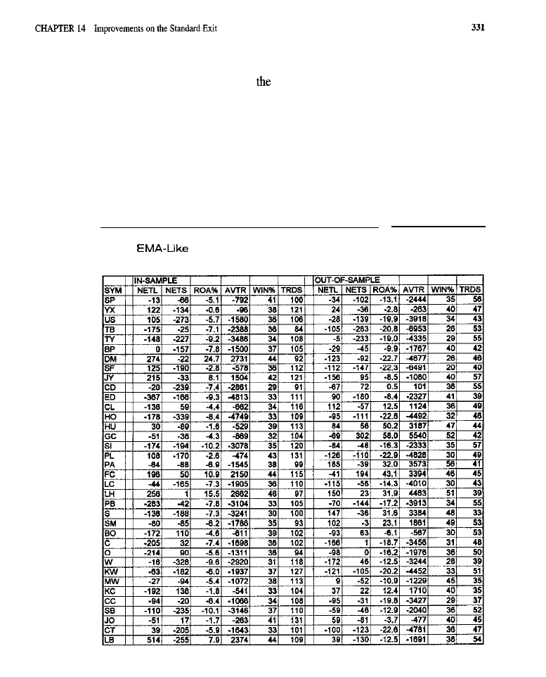
be seen.
In both samples, profits for
NYFE occurred on the long side, but not on
the short. Substantial profits occurred in both samples for Feeder Cattle-for long
and short positions in-sample, but only for short positions out-of-sample. Live
Hogs were profitable in both samples for both long and short positions. The
Deutschemark and Japanese Yen showed profits in-sample on the long side, but
had overall losses out-of-sample. The only exception was a small profit in the
Japanese Yen on the short side, but it was not enough to overcome the losses on
the long side. Lumber was strongly profitable on the long side in-sample, but only
T A B L E 1 4 - 7
Performance Broken Down by Market for Best Exit Strategy
with
Stop, Shrinking Profit Target, and Trade Time Limit
Extended to 30 Days

332
PART III The Study of Exits
had a very small profit on the long side out-of-sample. The two most outstanding
performers were Feeder Cattle and Live Hogs which, even despite the random
entries, could actually be traded. In-sample, there was a 10.9% annualized
for Feeder Cattle and a 15.5%
for Live Hogs. Out-of-sample, the
were 43.1% and 3
respectively. There were more profitable results
sample than in-sample, but this could easily have been due to the smaller sample
and fewer trades taken in the out-of-sample period.
CONCLUSION
Exits do make a big difference. By improving the risk management and
tar-
get elements in an exit strategy, losses can be cot and the risk-to-reward ratio can
be enhanced. The improvements in the tests above, however, were not as good as
expected. For example, although the best exit did appear capable of pulling prof-
its from random trades taken in two markets, no profits were obtained on the port-
folio, which is somewhat inconsistent with
earlier experiences (Katz and
McCormick, March 1998, April 1998) in which profitable systems were achieved
with random entries on the S&P 500. In those studies, exits were toned to the mar-
ket under examination, rather than keeping parameters constant across an entire
portfolio as done in the investigations above. This difference may account for the
poorer results in the current set of tests. In general, better results can be obtained
(albeit with much greater risk of curve-fitting and over-optimization) by tuning the
various components of a trading model to the specific characteristics of an indi-
vidual market. It should also be kept in mind that the tests conducted here were
fairly harsh with respect to transaction costs. For some markets (e.g., the S&P
commissions are almost negligible in terms of its typical dollar volatility,
and only slippage is a factor. However, in many smaller markets, great numbers of
contracts would have to be traded, causing the issue of commissions to become a
very significant consideration. In
earlier study, little or no transaction costs
were assumed, and a market in which the commission component would be fairly
small (i.e., the S&P 500) was examined. This factor may also have contributed to
the difference in findings.
When compared with the standard exit strategy used in the tests of entry
methods, which lost an average of $2,243 per trade and had a standard deviation of
$304, the best exit strategy thus far developed reduced the loss per trade to $1,236,
representing a reduction in loss per trade of over 44%. The reduction is substantial
enough that many of the better (albeit losing) entry models would probably show
overall profitability if they were combined with the best exit strategy.

WHAT HAVE WE LEARNED?
. Exits can make a substantial difference in overall performance. The
attempts described in this chapter have yielded an extra $1,000 per trade
over the standard exit strategy used in tests of entry models.
. Just as with entries, finding a good exit is like searching for a tiny island
of inefficiency in a sea of
market behavior. While such islands
there, they are difficult to find.

C H A P T E R I S
A D D I N G A l T O E X I T S
n this chapter, the modified standard exit strategy (MSES) is explored with the
addition of elements based on neural networks and genetics. In Chapter 11, neur-
al network forecasters were developed for use in generating entries. One of the
particular neural forecasters (the time-reversed Slow %K net) attempted to predict
whether tomorrow’s prices would be near the low or high end of the range of
prices that would occur over the next several days. This network can be added to
an exit strategy: If the net suggests that
market is near the top of its near-future
range and a long position is being held, it would probably he a good idea to exit
before the market begins to move down. Likewise, if the net forecasts a rising
market while a short position is being held, the trade should be exited before the
market begins to rise.
The first test conducted below explores the use of the time-reversed Slow
network (developed when studying entries) as an additional element to our
modified standard exit strategy. The net, which generates what might be called a
signal exit, cannot be used on its own for exiting because it will not always close
out a trade. This network was designed to provide entry signals. When it generates
a signal, the market is likely to behave in some expected manner. However, the
absence of a signal does not mean that the market will not do something signifi-
cant. When a position is being held, at some point an exit has to be taken, and that
action cannot be postponed until a significant event is finally predicted. The
MSES, in this case, guarantees that all trades have
money management pro-
tection and are exited after a given amount of time. The neural net, however, can
possibly improve the strategy by occasionally triggering an exit when a predicted
move against the trade is expected. In this way, the net may turn a certain propor-
tion of losing trades into winners.

The second batch of tests (one for the long side, one for the short) involves the
use of a genetic algorithm to evolve a set of rules generate a signal exit. The rules
are used in a manner similar to the way the net is used, i.e., to generate additional
exits,
context of the MSES, when the market is likely to reverse. The rule
templates and rule-generating methodology are the same as those used in Chapter
12, where evolved rules generated entries. In the current tests,
are evolved to
generate additional exits within the context of the
The rules are used as sig-
nal exits. The additional exits will, it is hoped, improve profitability by turning some
losses into wins and by killing other trades before they become larger losses.
More sophisticated exits can be developed using the techniques described above.
Although not explored in this chapter, a neural network could be evolved to produce
outputs in the form of placements for stops and limits, as well as for immediate, out-
right exits. Genetically evolved rules could also be employed in this manner.
used in the context of entries, neural networks proved to be fairly good
forecasters. It-sample, incredible profits were produced due to the accurate pre-
dictions. Out-of-sample, the nets yielded much better than chance results (albeit
not very profitable on the whole portfolio). Real predictive ability was demon-
strated. Using such forecasts to exit trades before the market reverses should
improve system performance, even if only by eliminating a small percentage of
bad trades. The same applies to the genetically evolved rules. However, when the
rules that produced entry signals for rare event trades are applied to exits, great
improvement in exit performance should not be expected. Given the nature of the
rules, only a small number of signals are likely to be generated, which means that
only small numbers of trades will be affected. If only a few of the large number of
trades that will be taken are improved, only a small overall benefit will be evi-
denced. Since the rules are being
for the tests below, more
of
exit opportunities may be found than were discovered for entry opportunities.
TEST METHODOLOGY FOR THE NEURAL EXIT
COMPONENT
The larger of the two best neural networks, trained to predict the time-reversed
Slow
are used. The preprocessing and forecast-generating logic are identical
to
discussed in Chapter
A series of predictions are generated using the
18-14-4-1 net (18 first-layer neurons, 14 neurons in
middle layer, 4 in the sec-
ond middle layer, and 1 output). The MSES is also used. Along with the exits pro-
vided by the MSES, an additional exit condition is being added: If the predicted
reverse Slow %K is greater than some threshold, indicating that the market is high
relative to its near-future price range, any long position is exited. Likewise, if the
net’s prediction indicates that
market is near the low of its neat-future price
range, by being below 100 minus the previous threshold, any short position is exit-
ed. Exits triggered by the neural net forecasts are taken at the close of the bar.

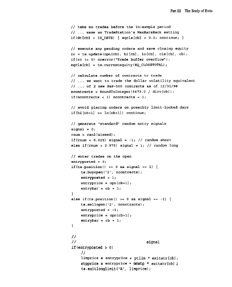
338
exit trades using the modified standard exit
strategy along with the neural
exit
(
initialization and exits for longs on entry day

339
(
initialization and exits for shorts on entry day
stpprice
+
The code fragment above implements the logic of the exit strategy. The para-
meters
and
are set to 4.5 and 1.5, respectively; these are the values
that gave the best overall portfolio performance (see Table 14-1, Chapter 14). The
thresh parameter, i.e., the threshold used to generate exits based on the neural fore-
casts, is optimized. The logic of the additional exit can be seen in the “if’ state-
ments that
the prediction of the network with the threshold and that post
an exit at close order based on the comparison. The parameter
thresh
is stepped
from 50 to 80 in increments of 2.
RESULTS OF THE NEURAL EXIT TEST
Baseline Results
Table 15-l contains data on the baseline behavior of the MSES. The threshold
set high enough to prevent any net-based exits from occurring. The numbers
in this table are the same as those reported in Chapter 14 (Table 14-I) for an

3 4 6
fixed stop and profit target. The abbreviations in Table
may be inter-
preted as follows:
whether the test was on the training or verification
sample (IN or OUT);
the total net profit on long trades, in thousands of
dollars;
the total net profit on short trades, in thousands of dollars; PFAC
= the profit factor; ROA% =
annualized return-on-account; ARRR = the
annualized risk-to-reward ratio; PROB = the associated probability or statistical
significance; TRDS = the number of trades taken across all commodities in the
portfolio; WIN% = the percentage of winning trades; AVTR = the average prof-
it/loss per trade; and TRDB = the average number of bars or days a trade
was held.
There was great consistency between in- and out-of-sample performance:
The average trade lost $1,581 in-sample and $1,580 out-of-sample; both samples
had 39% winning trades; and the risk-to-reward ratios were 1.46 in-sample and
1.45 out-of-sample.
Neural Exlt
Results
Table 15-2 is the standard optimization table. It shows the in-sample portfolio per-
formance for every threshold examined and the out-of-sample results for the
threshold that was the best performer during the in-sample period.
In-sample, an improvement in overall results was obtained from the use of
the additional neural network exit. The average trade responded to the threshold in
a consistent manner. A threshold of 54 produced the
best
results, with an average
trade losing $832. There were 41% wins and an annualized risk-to-reward ratio of
-0.87. The numbers represent a dramatic improvement over those for the baseline
presented in Table 15-l. Out-of-sample, however, no improvement was evident:
Performance was not too different from that of the optimal MSES without the
neural signal element. In the tests conducted using the neural net for entries, per-
formance deteriorated very significantly when moving from in-sample to
sample data. The same thing appears to have happened in the current test, where
the same net was used as an element in an exit strategy.
Baseline Performance Data for the Modified Standard Exit Strategy
to Be Used When Evaluating the Addition of a Neural Forecaster
Signal Exit
WIN%
IN
1.0000~
6
I
0.641
-21.61
391
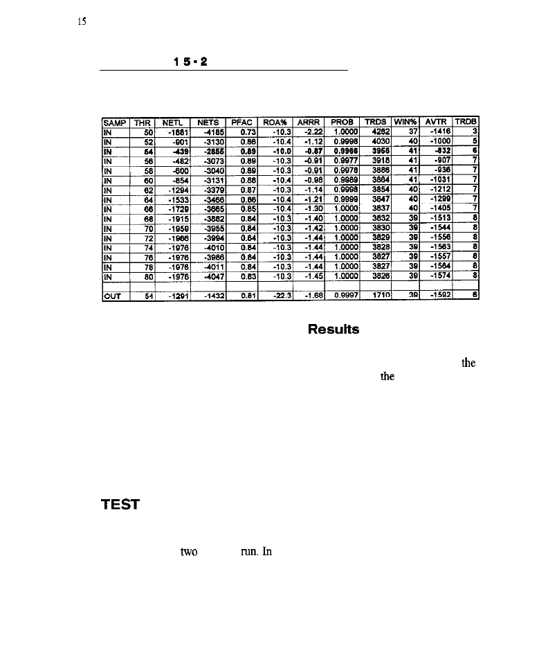
CHAPTER
Adding AI to Exits
341
T A B L E
Portfolio Performance of the Modified Standard Exit Strategy with an
Added Neural Signal Exit Evaluated over a Range of Threshold
P a r a m e t e r V a l u e s
Neural Exit Market-by-Market
Table 15-3 shows the performance data for the portfolio, broken down by market,
for the optimal MSES with the added neural signal
exit.
The results are for
composite exit with the best threshold value (54) found in
optimization pre-
sented
in
Table 15-2.
Live Hogs was the only market that was substantially profitable in both sam-
ples. A number of markets (e.g., the Deutschemark and Japanese Yen) showed
strong profitability in-sample that was not evident out-of-sample. On the long side,
the NYFE and Unleaded Gasoline were profitable in both samples. This could eas-
ily be a statistical artifact since, in-sample, a large number of markets had prof-
itable performance on the long side.
METHODOLOGY FOR THE GENETIC EXIT
COMPONENT
Since it is almost certain that different rules are required for the long side, as opposed
to the short side,
tests are
the first test, random entries are generated for
long positions using the standard random entry strategy. Any short trades generated
are simply not taken. Rules are genetically evolved for inclusion in the MSES for the
long positions. In the second test, only short entries are taken. Any long entries gen-
erated by the random entry strategy are ignored. An attempt is made to evolve rules
that work well as additional elements to the MSES for the short side.
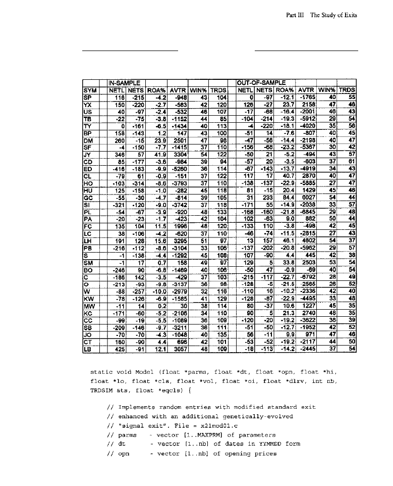
342
T A B L E I S - 3
Market-by-Market Performance for the Modified Standard Exit with a
Neural Signal Addition Using Random Entries

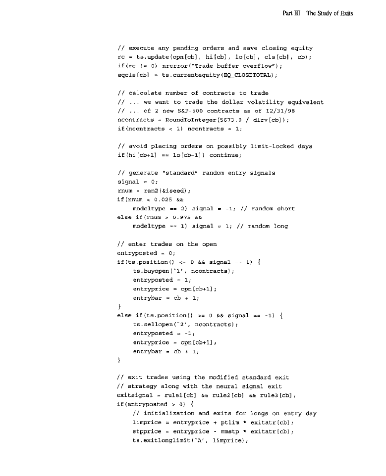

The code above shows the logic of both the entries and exits. The
parameter controls whether the longs or shorts are tested. Parameters
and
are for the profit target and stop (respectively). They are
at the same
optimal values used in the neural network test earlier, Each of the three rules is cal-
culated as a series of
TRUE/FALSE
values, and if all three rules are TRUE, a rule-
based exit signal
is generated. In the exit code, “if’ clauses have been
added. For example, an exit at the close is generated
exit signal is produced
by all three rules being
TRUE
=
TRUE).
The evolution of rules for the
long and short sides follow the same steps as in the chapter on genetics, in which
similar rules were evolved for use in entries. The same 12 parameter chromosomes,
broken into three genes (each specifying a rule), are employed, and there is no
change in that logic in the current test, Rules for the short side and for the long
side are produced by allowing 2,500 generations to pass (2,500 runs using
The top solutions for the longs and for the shorts are then tested
on both the in-sample and out-of-sample data.
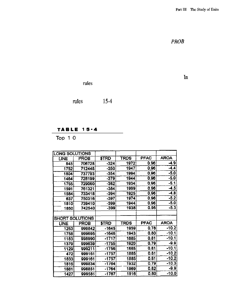
346
Top 10 Solutions with Baseline Exit
Table 15-4 shows the top 10 solutions found for the long side and for the short
side. In the table,
LINE
= the line or generation number;
= the probabili-
ty or statistical significance (the decimal point is omitted but implied in the for-
matting of these numbers);
$TRD
= the average dollars-per-trade;
TRDS = the
total number of trades taken;
PFAC
= the profit factor; and
AROA = the
annual-
ized return-on-account.
The best solution for the longs was discovered in the 845 generation of the evo-
lutionary process. For the short side, it was in the 1,253 generation.
contrast to the
situation when
were evolved for use in an entry model, none of the solutions
were profitable. However, Table 15-5 shows that when genetically evolved rule-based
exits were added, substantial improvement over the baseline was achieved.
The
in Table
were translated into plain language. The rules for
exiting a long position were as follows: If the close on the current bar is greater
Solutions from the Evolutionary Process
for Longs and for Shorts

than a
exponential moving average
of the closes, but is less than a
of the closes, and the current bar represents a
new high, then
exit the long trade. The rules seem to be searching for a situation in which the
longer trend is down, but a short-term
against the trend has occurred
and has reached a point where completion of the
is likely and the
longer-term downward trend will resume-a sensible point to exit a long position.
The rules for the short side suggest that an exit should occur if the close on the
current bar is greater than the
of the closes and a
simple mov-
ing average of the closes, and if the MACD
is
sloping down. The specific MACD
used employs a
for its faster moving average and a
for
its slower moving average. The idea encapsulated in these rules seems to be that
it is
to close
short positions if the market, when smoothed, still appears
to be moving down, but the most recent close broke above two moving averages,
indicating the market may be starting a new trend up.
Results of Rule-Based Exits for Longs and Shorts
Table
presents the performance data for best of the top 10 solutions (longs
and shorts) for the MSES with the addition of genetically evolved, rule-based
signal exits. Trades were entered randomly. The table is broken down into results
for long positions and results for short positions. It is further broken down by sam-
ple and test. Sample (IN or OUT) and test may be
(when the rules were not
used) or
RULE
(when the mles were. used).
On the long side, in-sample, the addition of the genetically evolved rule-based
exit substantially reduced the loss on the average trade from a baseline of $688 to $324.
The percentage of winning trades increased from 41 to 43%. The
T A B L E
Performance of the Modified Standard Exit Strategy with an Added
Genetically Evolved Rule-Based Signal Exit When Trades Are
Entered Randomly

reward ratio improved from -0.35 to -0.17. Out-of-sample, the benefit of the genet-
ically evolved mle-based signal exit was
but not quite as dramatically. The
loss on the average trade was cut from $1,135 to $990. The percentage of winning
increased from 39 to 41%. The risk-to-reward ratio improved slightly from
-0.61 to -0.60. Overall, adding the genetically evolved rule-based element to the exit
strategy worked. In contrast to the neural exit, the benefit was maintained out-of-mm
ple, suggesting that curve-fitting and over-optimization were not major issues.
On the short side, similar benefits were observed in both samples. In-sample,
the addition of the genetically evolved rule-based element reduced the loss on the
average trade from a baseline of $2,084 to $1,645. The percentage of winning
trades remained unchanged. Paradoxically, the annualized risk-to-reward ratio
worsened somewhat, going from 1.09 to 1.15. Out-of-sample, the loss on the
average trade dropped substantially, from $1,890 in the baseline test to $1,058,
when the rule element was active. The percentage of winning trades rose from 38
to
and the annualized risk-to-reward ratio improved, from 1.02 to -0.73.
Again, the addition of the genetically evolved rule-based signal exit to the MSES
worked and continued to work out-of-sample.
Market-by-Market Results of Rule-Based Exits
for Longs
Table 15-6 contains information regarding the market-by-market performance of
the MSES for the long side, with the added rule-based signal exit. Several markets
showed profitability in both samples: the NYFE, Light Crude, Unleaded Gasoline,
and Live Hogs. Other markets were profitable in-sample, but lost heavily
sample (and vice versa). The consistency between in-sample and out-of-sample
results was not high.
Market-by-Market Results of Rule-Based Exits
for Shorts
Table 15-7 shows the same market-by-market breakdown as in Table 15-6, but
only the short side is represented. More consistency was evident between in-sam-
ple and out-of-sample performances for the short side than for the long. Most
notably profitable in both samples was the Japanese Yen. Light Crude, Unleaded
Gasoline, Feeder Cattle, Live Hogs, Soybean Meal, and Coffee were also prof-
itable in both samples.
CONCLUSION
Several important points were demonstrated by the above tests. First, neural net-
works hold up less well in out-of-sample tests than do genetically evolved
based solutions. This is no doubt a result of the greater number of parameters

Market-by-Market Performance of the Modified Standard Exit with an
Added Genetically Evolved Rule-based Signal Exit When Tested
Using Random Long Trade Entries
involved in the neural network model, as compared with the rule-based models
being used. In
words, the effects of curve-fitting were damaging to the neur-
al network solution. Also discovered was the fact that the addition of a sophisti-
cated signal exit, whether based on a neural net or a set of genetically evolved
entry rules, can greatly improve an exit strategy. When
more robust, geneti-
cally evolved rules were applied, the performance benefits obtained persisted in
out-of-sample evaluations.
The neural network and the rule templates (but not the actual rules) that were
used in developing the signal exits were originally developed for inclusion in an
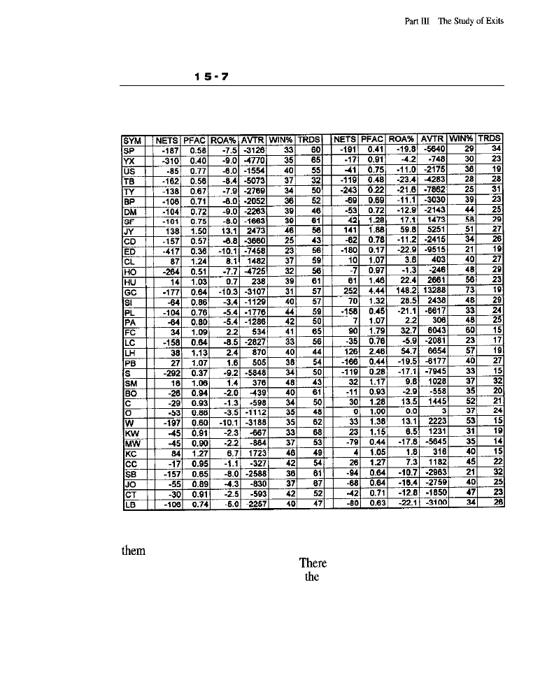
350
T A B L E
Market-by-Market Performance of the Modified Standard Exit with an
Added Genetically Evolved Rule-Based Signal Exit When Tested
Using Random Short Trade Entries
entry model. When the rules were used in an entry model, it was acceptable for
to generate rare event trades. In an exit strategy, however, rules that tire more
frequently would be more desirable.
is every indication that a set of rule
templates (and ways of combining
rules to obtain signals), specifically
designed for use in an exit strategy, would provide much better results than those
obtained here. The same should be true for neural networks.

WHAT HAVE WE LEARNED?
n
Curve-fitting can be bad not only when building entries, but
when
building exits.
n
Sophisticated technologies, including genetic algorithms, can be effec-
tively used to improve an exit strategy.
. Even crude efforts to improve exits, such as those carried out here, can
enhance profits by several hundred dollars per trade.

Conclusion
A
long road has been traveled since beginning the study of entry and exit strate-
gies. Sometimes the trip has been tedious and discouraging; at other times, stimu-
lating and surprising. As usual after extended journeys, the questions “What
knowledge has been gained?” and “How may that knowledge be applied?’ beg to
be answered. The
question will be addressed by a successively more detailed
examination of
results: going from discoveries made about the portfolio per-
formance of entire classes of models, to more specific model-order combinations,
down to an inspection of individual markets and how they are best traded.
The perspectives taken in the following discussions of what has been
achieved are analogous to views from an airplane flying at night. At first, the plane
is at a very high altitude: All that can be seen when looking down are large patch-
es of darkness (classes of models that are ineffective or lose) and some patches of
light (classes of models that, overall, work fairly well or, at least, perform better
than chance). This view provides a basic idea of which models are, overall, viable
relative to the entire portfolio of
The plane then descends. More detail is seen. It becomes evident that the
brightest spots are often formed by clusters of light having various luminosities
(model-order combinations that are, to one extent or another, profitable).
Occasionally the dark patches also contain small isolated points of brightness
(successful model-order combinations amid approaches that usually are ineffec-
tive). At this level, a number of dim areas can be seen as well (model-order com-
binations that are not profitable, but that have better than chance performance that
could be enhanced if combined with a good exit).

Finally, landing is imminent. It is possible to look inside the bright spots and
see their detail, i.e., the individual markets the various model-order combinations
trade best. The second question above can now
be
addressed: By identifying the
consistently profitable (across samples) model-order combinations and the mar-
kets best traded by them, a good portfolio trading strategy can be developed. At
this time, it will become clear that out of all the studies performed
the long
trip, enough has been
to assemble a lucrative portfolio of systems and
By way of demonstration, such a portfolio will be compiled and run with
the standard exit strategy.
THE BIG PICTURE
For this perspective, each class of entry model (e.g., all trend-following moving
average models, all breakouts, all small neural networks) was examined in its
entirety. All the tests for each model type were averaged. Out-of-sample and
in-sample performances were separately evaluated.
By far the best out-of-sample performer was the genetic model: Out of all the
models, it was the only one that showed a substantial profit when averaged over
all the different tests. The profit per trade was $3,271.
Next best, in terms of out-of-sample behavior over all tests, were the small
neural networks. The neural network models were broken down into those for
small and large nets because curve-fitting appeared to be a
serious
issue, especial-
ly affecting large nets. The breakdown was a natural and easy one to accomplish
because, in the tests, each model was tested with one small and one large network.
Out-of-sample, all the small neural networks taken together averaged a loss of
$860 per trade. This indicates a significantly
better than
chance entry in that ran-
dom entries produced an average loss of over $2,000, with a standard deviation of
slightly under $400.
Going down in quality, the next best overall approach involved
Altogether,
all tests
of
seasonality
models showed an average loss of $966 per trade.
Three of the moving average models (crossover, slope, and
followed the performance
of
seasonality. These models, when averaged
across tests, lost around $1,500 per trade, which is close to the $2,100.per-trade
loss expected when using random entries. In other words, the moving average
models were only marginally better than random.
All the remaining models tested provided entries that were very close to ran-
dom. Cycles were actually worse than random.
In-sample, the genetic models ($12,533 per trade), all the
neural
network
models (small, $8,940, and large,
and the breakouts ($1,537) traded
profitably. Out-of-sample, the genetic models continued to be profitable, the nets
were better than chance (although there was significant shrinkage in their perfor-
mance due to curve-fitting), and the breakouts deteriorated to chance (optimiza-
tion cannot be a factor in this case).

The next best performers in-sample were the support/resistance moving average
models ($300 loss per trade) and the seasonality models ($671 loss per trade).
Further down the ladder of best-to-worst performers were the lunar and solar
models, which lost $1,076 and $1,067, respectively. Losses in the $1,300 to
$1,700 range were observed for the moving average models. The oscillator and
cycle models exhibited losses of over $2,000 per trade; when taken as a whole,
these models were no better than chance.
It is interesting that the genetic model and the small neural network models
were the ones that held up out of sample. Such models offer great opportunities
for curve-fitting and tend to fail in out-of-sample tests and real trading.
Seasonality, which is only rarely the topic of articles, also exhibited potential. On
the other hand, the most popular methods (e.g., moving average, oscillator, and
cycle models) performed the worst, trading badly both in- and out-of-sample. The
breakout models are noteworthy in the sense that, taken as a group, they worked
well in the past; but, due to increased market efficiency, have since deteriorated to
the point where they currently perform no better than chance.
Table C-l contains the annualized return-on-account (the first line of each
order combination) and average dollars-per-trade (the second line of each model-order
combination) data for all the tests (all
and order combinations) conducted for
models using the standard exit strategy. The data presented
for portfolio performance
as a whole. The model descriptions (leftmost column) are the same as used elsewhere in
this book. The last six lines of the table contain data that can be used a baseline against
which the various entry models can be compared. The baseline data are derived from
using the random entry strategy
the
standard exit strategy.
ROA%
is the average return on account over several sets of random entries;
ROA%
is the
standard deviation of the return-on-account.
Mean
is the average dollars-per-trade
over several sets of random entries; and
is the standard deviation of the
dollars-per-trade.
Breakout models had the unique characteristic of being consistently profitable
in-sample across almost every model-order combination tested. Except for the
volatility breakouts, these models performed much better than chance, albeit not
profitably, out-of-sample; i.e., the loss per trade was under $1,000, sometimes under
$300 (the average loss to be expected was around $2,000 with random entries). In
other words, the breakouts, taken together, were better than random. However,
of-sample, the volatility breakouts did much worse than chance: With at-open and
on-stop orders, the model lost more than $5,000 per trade, as though the market’s
current behavior is precisely designed to make these systems costly to trade.
The trend-following moving average models (crossover and slope) all per-
formed slightly better than chance in-sample: They all lost rather heavily, but the
losses were almost always less than $2,000. None of the systems, however, did
very well. Out-of-sample, the picture was somewhat more variable, but had the
same flavor: Most of the models were somewhat better than chance, and one or
two were much better than chance (but still not profitable).
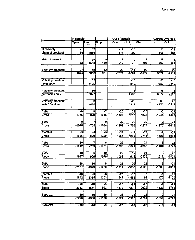
3 5 6
T A B L E C - l
Summary of Portfolio for All Entry Models Tested with All Order Types
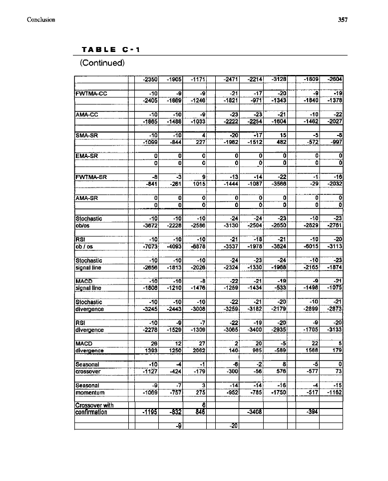
- 1 0
- 7
- 1 4
- 2 1
2 0
- 4
- 5
- 1 5 1 2
1 8 7 7
- 1 0 8 1
Crossover with
- 1 0
- 2
- 2 3
1
- 7
- 1 4
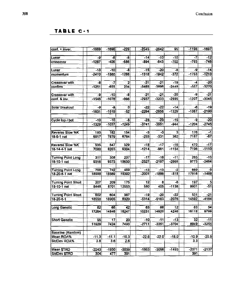
(Continued)

The countertrend moving average models were more variable than the
following ones. Many of them showed much smaller losses or even small profits,
in-sample. A similar picture was seen out-of-sample, especially with the simple
moving average support/resistance model.
Except for the MACD divergence model, which behaved differently from the
others, oscillators performed very poorly. There was a lot of variability, but on the
whole, these models gave per-trade profits that were worse than expected by
chance both in-sample and out-of-sample. The RSI overbought/oversold model
was the worst of them all. In both samples, it provided staggering losses that were
(statistically) significantly worse than those that would have been achieved with a
random entry.
The seasonal models, on the whole, were clearly better than chance. Although
only one of these models actually provided profits in both samples, two of them
were profitable out-of-sample, and several had only very small losses (much less
would be expected by chance using random entries) across samples.
The basic lunar model had mixed findings. Most of the in-sample results
were slightly positive when compared with chance (the random entry), but not
profitable. The basic crossover model, however, was decidedly biased above
chance in both samples.
Although the solar models performed slightly better than chance in-sample,
they were mixed and variable out-of-sample. This was also true for the cycle models.
However, the cycle models, when using entry at open or on limit, actually performed
significantly worse in recent years than a random entry. As with breakouts, the find-
ings are not due to optimization; significant curve-fitting was only detected with the
genetic and neural network models. Because of the tremendous sample involved in
the portfolio, the optimization of one or two parameters, necessary for most models
(other than the genetic and neural ones), had minimal curve-fitting effect.
Surprisingly, the neural network models showed a fairly consistent bias to per-
form better than chance out-of-sample. In-sample, of course, performance was stel-
lar across all tests. There was shrinkage (evidence of curve-fitting), but the shrinkage
was not complete, leaving some predictive utility in the out-of-sample data.
The results for the genetically evolved rules were the best. In-sample, per-
formance was excellent, Out-of-sample, performance was exceptional for models
involving long positions.
Summary
Many of the models described as significantly better than chance (i.e., better than
what would be produced by a random entry) would likely become profitable if cou-
pled with a better exit strategy. In Part III, it was evident that when tested with
dom entries, the use of a good exit could bolster profits (or cut losses) by about
per trade. This means
a good exit, some of the entry models that had loss-
es of several hundred dollars could be brought into positive, profitable territory.

As mentioned above, the journey was a long one, sometimes tedious and dis-
couraging. However, this birds-eye view revealed that a lot of potentially profitable
entry models were indeed discovered. There were also a number of surprises: Despite
terrible reputations and dangerous tendencies toward curve-fitting, the neural network
and genetic models were the best performers when tested with data that was not used
in training or evolving. Another surprise was that
of the most popular trading
approaches, e.g., moving-average crossovers and oscillator-based strategies, turned
out to be among the worst, with few exceptions. The results of the cycle models were
also revealing: Because of their theoretical elegance, better-if not ideal-perfor-
mance was expected. However, perhaps due to their popularity, poor performance
was observed even though the implementation was a solid, mathematical one.
POINTS OF LIGHT
The portfolio performance of each model was examined for each of the
order
types (at open, on limit, and on stop). Out-of-sample and in-sample performances
were separately evaluated.
The out-of-sample performance was, by far, the best for the long-side genet-
ic models. Entry at open was especially noteworthy, with a 64.2% in-sample return
and 41.0% out-of-sample. The same model was also profitable with entry on limit
and on stop, yielding very high dollars-per-trade profits, although small numbers
of trades (easily increased with more elaborate models of this kind).
In terms of out-of-sample performance, the next best specific model-order
combination was the seasonal crossover with confirmation using entry on stop. Like
the long genetic models, this one was significantly profitable in both sampling peri-
ods: in-sample, $846 per trade, with a 7.4% return; out-of-sample, $1,677 per trade,
with a 9.5% return. Other seasonal models also did okay, with out-of-sample profits
being made using the simple seasonal crossover model,
Next down the list was the short turning-point model that used the small 16-
10-1 network. This model was profitable in both samples across all orders:
sample, at open, a 9.3% annualized return, with $580 per trade; in-sample, a
35.2% return and $8,448 per trade profit.
While still on the subject of neural networks, the reverse Slow %K model
was a profitable performer, especially when a stop order was used. Out-of-sample,
the annualized return was
with $362 per trade. In-sample, there was a 22.5%
return, with a $6,764per-trade profit. Note the large shrinkage from in-sample to
out-of-sample for these models: While this is evidence of curve-fitting, enough
real curves were caught for profits to be made in the verification sample.
Another model that produced profits in both samples was
MACD diver-
gence model, especially with entry on limit. This model had a 6.1% annualized
return, out-of-sample, and a
profit. In-sample, the figures were a
6.7% return and a $1,250
per trade.

Conclusion
361
Finally, among the models that were profitable in both samples was the sim-
ple moving-average
model with entry on stop: It took 6.4%
out
of the market, with $482 per trade, out-of-sample; and
with $227 per trade,
in-sample.
Almost all other models lost money out-of-sample, and often in-sample, as
well, The only exception was the volatility breakout model restricted to the curren-
cies, which performed fairly well. Out-of-sample, it had an 8.5% return and made
$2,106 per trade. In sample, it had a 12.4% return, with $3,977 profit per trade.
Summary
Even though
most
of the other model-order combinations lost out-of-sample, in
many cases, the losses were much less than would be expected with a totally ran-
dom entry. In a number of instances, however, they were worse.
It seems evident that there are a number of models that, although not ideal
and in need of further development, do yield profitable trading that holds up in a
verification sample and yields reasonable statistics.
L O O K I N G I N T O T H E L I G H T
Until this point, only tests and models that operate on the whole portfolio have
been discussed. In the course of the tests, many observations were made regarding
the performance of specific models when trading individual markets. A recurrent
observation was that certain models seem to trade certain markets well, while
other models trade them poorly. Some markets just seem to be difficult to trade,
regardless of model. There is no doubt that by selecting a number of the better
models, and then selecting markets that these models trade well, a portfolio of sys-
tems to trade a portfolio of markets could be assembled. Therefore, good
market combinations were selected from among the tests conducted in this book.
No optimization of model parameters was performed.
A portfolio was assembled on the basis of in-sample statistical significance.
The intention was to
one good model-order combination for each of the mar-
kets in the portfolio. If there were several potential models for a given market, the
additional ones were discarded based on such things as model complexity (the
more complex the model, the less it was trusted), mediocre portfolio performance,
and other similar factors. The specific model-order combinations spanned the
entire spectrum of models and orders tested, with various oscillators, moving aver-
ages, lunar and solar models, and seasonal and neural network models being rep-
resented; genetic models, however, were not included. In the current tests, the
particular genetic models that were evolved only
traded rare
events. For those
sample markets that performed well, there were generally no out-of-sample trades.
The profitable out-of-sample behavior was achieved on almost a totally different
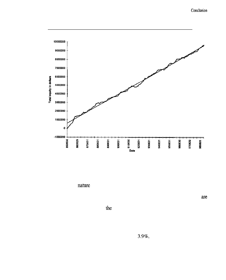
3 6 2
F I G U R E C - l
Equity Growth for Multiple-System and Market Portfolio
set of markets than the in-sample behavior of the model. This does not mean that
the out-of-sample performance was bad while the in-sample performance was
good, but rather that most markets simply did not trade in one sample if they did
in the other. The low number of trades observed with the genetic models was due
to the specific
of the particular rule templates and the ways in which the
individual rules were combined to obtain buy and sell signals. With some changes
in the rule templates, especially in the number of rules used and in how they
combined, the pattern of rare event trading can be entirely altered.
There were times when
preferred kind of model was not available for a
given market. In such cases, models were examined that performed poorly on a
whole-portfolio basis, but that did trade one or two difficult markets acceptably.
For example, the RSI overbought/oversold model with entry on limit was a poor
performer on a portfolio-wide basis. However, this model traded Gold and Silver
reasonably well. It pulled returns of 27.3 and
annualized, on the in-sample
data, with average trades of $9,446 and $4,164, respectively. Out-of-sample, the
system pulled 23.6% out of the Gold and 51.7% out of the Silver markets, with
average
trades
yielding $12,194 and $24,890, respectively.
One of the large neural networks that appeared to be highly over-optimized
was used for the three wheat markets-markets that did not trade at a statistically
significant level with any of the other models. The large, long-side, turning-point
network with entry on limit, however, had high statistical significance when trad-
ing each of the wheats, pulling more than 40%
from each, and more than
$15,000 per trade. The amazing thing is that, out-of-sample, despite the size of the
net and the degree of curve-fitting seen on its portfolio performance, the model
pulled in no less than
with $5,000 per trade, from each of
wheats.
The cycle model, which worked well on hardly any market, did trade the
S&P 500 profitably-returning
with an average in-sample trade of $4,613,
and 21.4% with
profit out-of-sample. It should be noted that a
cycle model was found to trade the
successfully in the tests reported in
our earlier study (Katz and McCormick, May 1997).
Once each market was paired with a good model-order combination, the per-
formance data were analyzed, both in- and out-of-sample, for each of the markets.
An equity curve was prepared that covered
periods (see Figure C-l). Returns
and statistical significance were calculated for the multiple-model portfolio, both
in-sample and out-of-sample. It was surprising to discover that the out-of-sample
performance data revealed a return-on-account of 625% annualized! A manifesta-
tion of the Holy Grail? Because model-market combinations were selected on the
basis of their in-sample statistical significance, the 544% annualized in-sample
was not unexpected. The probability of obtaining an in-sample profit as
large as that is less than 1 in
(i.e., 3 X
Even if
massive amounts of optimization, with tests of tens of thousands of combinations,
took place, the results would still be extremely significant, in a statistical sense.
Out-of-sample,
probability of finding a risk-to-reward ratio or annualized
return as good as that observed is less than 1 in 40 million. Again, even corrected
for extensive optimization, the results would still be of extreme statistical signifi-
cance. In fact, no out-of-sample optimization took place. In-sample, the systems
were only optimized on the entire portfolio. Model parameters were never adjust-
ed for the selected markets on which the models were to be traded. And only the
minimal standard exit strategy was used. Performance could be very substantially
improved using the best of the exits found in Part III.
These findings demonstrate that while most systems do not work and most
tests show losses, a sufficiently extensive search (as conducted in this book) can
discover enough
do work to put together a portfolio trading strategy capable
of producing nothing less than stellar results.

Conclusion
COMPANION SOFTWARE AVAILABLE
We invite all readers to visit
at:
or
to e-mail us at
Those who wish
replicate and expand on
research may obtain
copy of the C-Trader Toolkit (the software. required
the code presented in
this book) from
at
A CD-ROM is
also available for the nominal cost of $59.00. It contains the following:
Complete code for every method tested in this book
. Commodities data from Pinnacle
. Spreadsheets containing all optimization data, market-by-market analy-
ses, equity
figures, and tables
The C-Trader Toolkit, which includes the C+ Trading Simulator,
(the genetic optimizer), the Portfolio Simulation Shell, and
related manuals
Address
City
Phone: home
Company
state
Country code
office
The companion CD-ROM: $59.00 X
copies $
Numerical Recipes in C:
994
page book $54.95 X ___ copies
software IBM disks $39.95 X
copies
for CD only: add $3.50 per copy US, $7.50 outside US
$
for
Recipes: add $12 US, $35 outside US
$
S A L E S T A X
(NYS residents add
for your county
$
CHECK
Enclosed is my check “
I
money order (U.S. only)
my
below)
#
expiration
signature
order
“
I
mail, phone, fax it to:
SCIENTIFIC CONSULTANT SERVICES, INC.
Phone fax:
20 Stagecoach Road, Selden, New York 11784
631-696-3333
A P P E N D I X
References and Suggested
Reading
Alexander,
1993). “Trade with Moving Averages.” Technical
a n d
Commodities, pp.
I.
Appel, Gerald (1990). The Advanced Moving Average Convergence-Divergence Trading Method.
Videotape and manual distributed by
New York
Scott (September 1996). “The COT Index.” Technical Analysis
of
and Commodities,
pp.
S c o t t ( O c t o b e r 1 9 9 6 ) . “ P o r k B e l l i e s a n d t h e
Index.” T e c h n i c a l A n a l y s i s
Commodities, pp.
Bernstein,
(1995). T r a d e Y o u r W a y
Riches. MBH Commodity Advisors, Inc. (l-800-457-
0X25), 1995.
William (January 1993). “Stochastic Momentum:’ T e c h n i c a l A n a l y s i s o f S t o c k s a n d
Commodities. pp.
Burke, Gibbons (May 1993). “Good Trading Matter of Breeding?” Futures Magazine, pp.
Center for Solar and Space Research, Yale University (1997). Sunspot Predictions. Release
by Virtual Publishing Company.
S. (March 1992). ‘Adapting Moving Averages
Market Volatility.” Technical
Analysis
of
and Commodities, pp.
Davies, D.
(June 1993). “Cyclical Channel Analysis and the Commodity Channel Index.”
Technical Analysis of Stocks and Commodities, pp.
Davis, Lawrence
(1991). Handbook of Genetic Algorithms. New York: Van Nostrand Reinhold.
John (March 1989). “Moving Averages and Smoothing Filters,” Technical Analysis
of
Stocks
a n d C o m m o d i t i e s , pp.
Gauquelin, H., Gauquelin, R., and Eysenck,
B. G. (1979). “Personality and Position of the Planets
at Birth: An Empirical Study.”
Journal
of
Social
Clinical Psychology, Vol. 18,
Goedde, Richard (March 1997). “Timing a Stock Using the Regression Oscillator.” Technical
Analysis of Stocks and Commodities, pp.
(November 1991). “The Seasonal Cycle.” Technical Analysis of
and
Commodities, pp.
Paul G. (1966).
2d
New York:
Wiley
Sons.
365

366
Holland, John
A d a p t a t i o n i n
a n d
Systems. Ann Arbor: The University of
M i c h i g a n P r e s s .
Mark (1999). “Finding the Best Data.” C o m p u t e r i z e d T r a d i n g . Mark
(Ed.). New York:
New York Institute of Finance/Prentice Hall, pp. 355-382.
Katz, Jeffrey Owen (April 1992). “Developing Neural Network Forecasters for Trading.”
Analysis of
and Commodities, pp.
Katz, Jeffrey Owen, and McCormick, Donna L. (1990). Calendar Effects Chart. New York:
Scientific Consultant Services.
Katz. Jeffrey Owen, and McCormick, Donna L. (March/April 1993). “Vendor’s Forum: The
Evolution of N-TRAIN.”
Katz, Jeffrey Owen, and McCormick, Donna L. (1994). “Neural Networks: Some Advice to
Beginners.” Trader’s
Resource Guide, Vol. II, No. 4, p. 36.
Katz, Jeffrey Owen. and McCormick, Donna L. (July/August 1994).
a n d I t s U s e i n
Trading System Development.”
pp.
1 .
Katz, Jeffrey Owen, and McCormick, Donna L.
“ I n t r o d u c t i o n t o A r t i f i c i a l I n t e l l i g e n c e :
Basics of Expert Systems, Fuzzy Logic, Neural Networks, and Genetic Algorithms.”
T r a d i n g ,
and R. A.
Chicago:
P u b l i s h i n g ,
3 - 3 4 .
Katz, Jeffrey Owen, and McCormick, Donna L.
“Neural Networks in Trading.”
Trading, J.
and R. A. Klein
Chicago:
Publishing, pp.
Katz, Jeffrey Owen, and McCormick, Donna (November 1996). “On Developing Trading
Systems.” Technical Analysis of Stocks and Commodities, pp.
Katz, Jeffrey Owen, and McCormick, Donna L. (December 1996). “A Rule-Based Approach to
Trading.” Technical
of Stocks
Commodities, pp. 22-34.
Katz, Jeffrey Owen, and McCormick, Donna L. (January 1997). “Developing Systems with a
Based Approach.” Technical Analysis of Stocks and
pp. 38-52.
Katz. Jeffrey Owen, and McCormick, Donna L. (February 1997). “Genetic Algorithms and
Based Systems.” Technical
of Stocks and Commodities, pp.
Katz, Jeffrey Owen, and McCormick, Donna L. (April 1997).
and Trading.” Technical
of Stocks and Commodities,
Katz, Jeffrey Owen, and McCormick, Donna L. (May 1997). “Cycles and Trading Systems.”
Technical Analysis of Stocks and
pp.
Katz, Jeffrey Owen, and McCormick, Donna L. (June 1997). “Lunar Cycles and Trading.”
Analysis of
and Commodities, pp.
Katz, Jeffrey Owen, and McCormick, Donna L. (July 1997). “Evaluating Trading Systems with
Statistics.” Technical Analysis of Stocks and
pp.
Katz, Jeffrey Owen, and McCormick, Donna L. (August 1997). “Using Statistics with Trading
Systems.”
A n a l y s i s
p p . 3 2 - 3 8 .
Katz. Jeffrey Owen, and McCormick, Donna L. (September 1997). “Sunspots and Market Activity.”
Technical Analysis
of
Stocks and Commodities pp.
Katz, Jeffrey Owen, and McCormick, Donna L. (November 1997). “Adding the Human Element to
Neural Nets.” Technical Analysis
Stocks
Commodities, pp. 5264.
Katz, Jeffrey Owen, and
Donna L.
1998). “Exits, Stops and Strategy.”
Technical
of Stocks
Commodities pp.
Katz, Jeffrey Owen, and
Donna L. (March 1998). “Testing Exit Strategies,”
Analysis of
and Commodities, pp.
Katz, Jeffrey Owen, and McCormick, Donna L. (April 1998). “Using Trailing Stops in Exit
Strategies.” Technical Analysis
and Commodities, pp. 86-92.
Katz. Jeffrey Owen, and McCormick, Donna L. (May
“Using Barrier Stops in Exit
Strategies.” Technical
of Stocks and
pp. 63-89.

Katz, Jeffrey Owen. and McCormick, Donna L. (July
“Barrier Stops and Trendlines.”
Technical Analysis of Stocks and Commodities, pp.
Katz, Jeffrey Owen, and McCormick, Donna L. (1999). “Case Study: Building an Advanced Trading
System.” Computerized
(Ed.). New York: New York Institute of
F i n a n c e / P r e n t i c e H a l l , P p . 3 1 7 - 3 4 4 .
Katz, Jeffrey Owen, and McCormick, Donna L.
1999). “Trading Stocks with a Cyclical
System.” Technical Analysis of Stocks and
Pp.
Katz, Jeffrey Owen, and
F. James (April 1975). “Primary
A n O b l i q u e
Rotation to Simple Structure.” Journal
of
Behavioral Research, Vol. pp.
Knight, Sheldon (September 1999). “How Clean Is Your End-of-Day Data?”
Futures Magazine,
64.
Joe
994).
The Trading Systems Toolkit, Chicago:
Publishing.
and Klein, R. A. (Eds.). (1995).
Trading. Chicago:
Publishing.
Louis M. (December 1994). “Trading Markets with
Technical Analysis of Stocks
and Commodities, pp.
K e v i n ( 1 9 9 9 ) . “ F i n a n c i a l D a t a
Sources.” Computerized Trading, Mark Jurik (Ed.). New
York: New York Institute of Finance/Prentice Hall, pp. 345-354.
Masters, Timothy (1995). Neural, Novel
lime Series Prediction. New York:
John
Wiley Sons.
Mayo,
and Eysenck, H. J. (1978).
Empirical Study of the Relation between
Astrological Factors and Personality.” The Journal of Social
Psychology, Vol. 105, pp.
229-236.
Lawson (January 1994). “Price/Oscillator Divergences.”
Technical Analysis of
Stocks and Commodities, pp. 95-98.
Meibahr, Stuart (December 1992). “Multiple Length
Technical Analysis of
Commodities, pp.
Meyers, Dennis (May 1997). “Walk Forward with the Bond XAU Fund System.”
of
Stocks and Commodities, pp. 16-25.
Montgomery, Douglas C., and Peck, Elizabeth A. (1982).
Linear Regression
Analysis. New York: John Wiley Sons.
Patrick G.
1994). “Smoothing Data with Less Lag.” Technical
of
Stocks
Commodities, pp.
Murphy, John
(1991).
Technical
Trading Strategies
for
the Global Stock,
Bond, Commodity and Currency Markets. New York: John Wiley
Sons.
Myers, Raymond H.
(1986). Classical and Modem Regression with Applications. Boston:
Oliver, Jim (March 1994). “Finding Decision Rules with Genetic Algorithms.”
AI
32-39.
Robert
(1992). Design,
and
of Trading
New York: John Wiley
S o n s .
Press, W.H.,
B.P.,
S.A., and
W.T. (1986).
Numerical Recipes: The
of Scientific Computing. Cambridge, England: Cambridge University Press.
Press, W. H.,
S. A., Vetterling,
and
B. P. (1992).
Numerical Recipes in
Cambridge, England: Cambridge University Press.
Price, Kenneth, and Storm,
(April 1997). “Differential Evolution.”
Journal. pp.
18-24.
Ruggiero, Murray A., Jr. (April 1994). “Getting the Lag Out.”
Futures Magazine, pp.
Ruggiero, Murray A., Jr. (October 1996). ‘Trend-Following Systems: The Next Generation.”
Futures
Magazine.

368
and Suggested Reading
Murray A., Jr. (1997).
Cybernetic Trading. New York: John Wiley Sons.
Murray A., Jr. (May 1998). “Unholy Search for the Grail.”
Magazine.
Jack (October 1992). “Selecting
the Best Futures for Computer Testing.” Technical
Analysis of Stocks and Commodities, pp. 65-71.
William
(Fall 1994). ‘The
Ratio.” Journal of
Management.
Space Science Institute (1996). ‘A Magnetic
R i p s t h r o u g h
Atmosphere.” A news
release on their
site:
Star, Barbara (July 1993). “WI Variations.” Technical Analysis
Commodities, pp.
David (1999). “Evaluating Trading Performance.”
Computerized Trading. New Jersey:
New York Institute of Finance/Prentice Hall, pp.
Sweeney, John (1993). “Where to Put Your Stops.” Technical Analysis
of
and Commodities
(Bonus Issue), pp.
Sweeney, John (April 1998). “Applying Moving Averages.”
Technical Analysis
Stocks and
Commodities, pp.
Tilley, D.L. (September 1998). “Moving Averages with Resistance and Support.”
Technical Analysis
of
Commodities, pp. 62-87.
Robert R., and Turban,
(Eds.) (1993). Neural
in Finance and Investing.
Chicago:
Publishing.
White, Adam (April 1993). “Filtering Breakouts.”
Technical
of
and Commodities,
pp.
Wilder,
Welles (1978).
New
in Technical Trading Systems. Trend Research.
Williams, Larry (1979).
Z Made One Million Dollars
Year Trading: Commodities. New
York: Windsor Books.
and de la
Michael (June 1994).
Genetic Algorithm System for Predicting the
Technical Analysis of Stocks
pp. 5864.

I N D E X
AI (see Genetic algorithms,
networks)
All-past-years technique,
Analysis, 39
Analytic
39,
48
Annealing, 38
Annualized risk-to-reward ratio
Artificial
(see Genetic algorithms,
Neural networks)
(See
rhythms)
Author’s conclusions, 353-363
Average directional
index
Average
86
Back-adjustment,
Bad curve-fitting,
Band-pass
207
287
Bars, 109
Basic
mode,:
lunar activity,
Basic
model:
activity, 194.
1 7 0 ,
154
Best exit strategy (market-by-market results),
solution to a problem. 30
Beta weights, 55
1 3 4
Bonneville
Market
Borland, 24.25
Bottom
mode,,
Bouncing tick, 25
analysis
b y
1 0 7
Breakout models
breakout
channel breakouts,
of breakouts,
85
only channel breakouts,
currencies only,
102
orders,
highest
low breakouts, 92-97
interactions.
lessons
107,
long positions only,
of results,
testing, X5-104
types of breakouts, 83. 84
volatility breakout variations.
volatility
97-100
203
force optimizers, S-34.47
Burke. Gibbons, 257
filters, 206, 207
c++
26
C++
Optimizer, 49
C-Trader toolkit, 14,
114,214
Calendar effects chart, 154
288
CCI
channel
135,
CD-ROM,
155,181
limit
61.68
S.,
breakouts,
258
clipping, 164
Close only
breakouts,
Code
cycle-based entries,
dynamic stops,
genetic
262-268
genetic exit
342-345
activity.
moving
average models.
3 0 2 3 0 5
369

370
listings (Cont.):
exit strategy, 337-339
233-237
oscillator-based entries.
target (fixed stop). 311-313
slow %K
233-237
shrinkage
target, 326328
exit strategy
turning-point
241,242
Commodities channel index
136
Commodities
I
software
364
227
Conclusions, 353-363
Confidence interval, 60
model:
lunar activity, 182,
156, 173
8
Continuous contract, 3
125
Correlational statistics, 52
Cost function, 30
Counter-trend moving
entry models,
function, 60
Critical threshold exits, 283
genetic algorithms, 258,259
activity. 181,
155, 156
(See
Basic
Crossover-with-confirmation
lunar activity, 182,
196
156. 171-173
C-Trader toolkit, 14, 15,
Cumulative t-distribution, 58, 59
bad. 54
54
neural
230,255
optimization. and 54-57
Cycle, 203
Cycle-based entries,
206,207
characteristics.
214
code testing,
filter banks.

Entry methods
dollar volatility equalization. 78-81
genetic algorithms.
good
lunar/solar phenomena.
moving average
networks,
in
153-177
standard portfolio, 81. 82
standardized exits, 77.78
International.
model building
Genetic
47.49
Exit strategies,
287
best exit
trading, 289
critical threshold exits, 283
dynamic AIR-based stop, 322, 323
dynamic stops, 316-324
extended
limit, 328
fined
311-316
gunning, 288
low stop, 322
importance, 281,282
on
exit,
dynamic stop. 323,324
modified standard
money
protective stops. 288. 289
random
model, 291,292
shrinking
288
slippage,
standard exit
time-based
286
volatility
287
76
Exponential moving average,
112
Extended time
(exit strategies),
328
Eysenck,
Eysenck,

372
HHLL breakouts, 92-97
HHLL stop, 322
High-pass
206
Highest
low
92-97
Highest
low stop, 322
Histograms.
Holland,
optimizers, 3
Individual
data, 3
statistics (see Statistics)
data.,
48.49
Mathematics and Statistics
pricing data, 4
Inversions,
(See also
mode,)
Doily,
Jeffrey
154,
181, 197,199,
Klein,
227
Knight,
Lag, 110
Lane’s stochastic,
Leave-one-out
I., 227
orders,
Linear band-pass
programming,
Lunar
solar rhythms. 75.76,
basic crossover mode,,
basic momentum mode,, 194, 195
code listing.
model with
195,
with
and
196
generating lunar entries,
182
activity,
analyses, 196, 197
Lunar and solar rhythms
test
results.
series,
Louis
134
MACD divergence
MACD Histogram
134
MACD signal
models,
Timothy, 48.49
The, 48
258
MM-LAB, 48
Maximum
203.204
Maximum
spectral analysis (MESA), 203
Mayo,
179
199.
W. Lawson, 136
58
Mean squared deviation, 58
139
dynamic
323,324
203
MESA96.76
15, 26
exponential moving average
323,324
exit
Momentum, 133,
(See also Basic
mode,)
Money management,
Money management
283,284
Money
stop, 78
Monte
simulations, 67
Moving average, 109
Moving average convergence divergence oscillator
134
Moving
crossover,
Moving average models. 74,
vend filters,
code listing,
counter-trend models, 113,
equity
lag,
lessons
132
moving average,

Pascal,
14.41
optimizers,
to
45.46
analytic,
force, 32-34
choosing
right one, 48.49
failure of,
genetic. 35-38
used,
implicit, 3
4 3 4 5
sample size,
annealing, 38.
sources of
ascent, and, 39
of, 43-45
types, 3141
user-guided optimization, 34, 35
43.45
what
do. 29.30


Wyszukiwarka
Podobne podstrony:
Gale Group Encyclopedia of World Religions Almanac Edition Vol 6
Encyclopedia of Explosives and Related Items Volume 02
Encyclopedia of Legal Psychoactive Herbs
Kingdom of Denmark Strategy for Arctic 2011 2020
Encyclopedia of Computer Scienc Nieznany
Data Modeling Object Oriented Data Model Encyclopaedia of Information Systems, Academic Press Vaz
Cho Chikun's encyclopedia of life and death part three a
Cho Chikun's encyclopedia of life and death part one ele
ICWR Forex Trading Strategy
LEAPS Trading Strategies Powerful Techniques for Options Trading Success with Marty Kearney
encyclopedia of herbs and mind enhancing substances 2000 group
Encyclopedia of Explosives and Related Items Volume 03
80 Trading strategies id 47247 Nieznany (2)
Encyclopedia of Explosives and Related Items Volume 07
więcej podobnych podstron