L

L

E

E

C

C

T

T

U

U

R

R

E

E

7

7

S

S

T

T

R

R

E

E

S

S

S

S

I

I

N

N

F

F

L

L

U

U

I

I

D

D

S

S

.

.

C

C

O

O

N

N

S

S

T

T

I

I

T

T

U

U

T

T

I

I

V

V

E

E

R

R

E

E

L

L

A

A

T

T

I

I

O

O

N

N

A

A

N

N

D

D

N

N

E

E

W

W

T

T

O

O

N

N

I

I

A

A

N

N

F

F

L

L

U

U

I

I

D

D

.

.

M

M

A

A

T

T

H

H

E

E

M

M

A

A

T

T

I

I

C

C

A

A

L

L

M

M

O

O

D

D

E

E

L

L

F

F

O

O

R

R

I

I

N

N

T

T

E

E

R

R

N

N

A

A

L

L

F

F

O

O

R

R

C

C

E

E

S

S

I

I

N

N

F

F

L

L

U

U

I

I

D

D

S

S

.

.

S

S

T

T

R

R

E

E

S

S

S

S

T

T

E

E

N

N

S

S

O

O

R

R

.

.

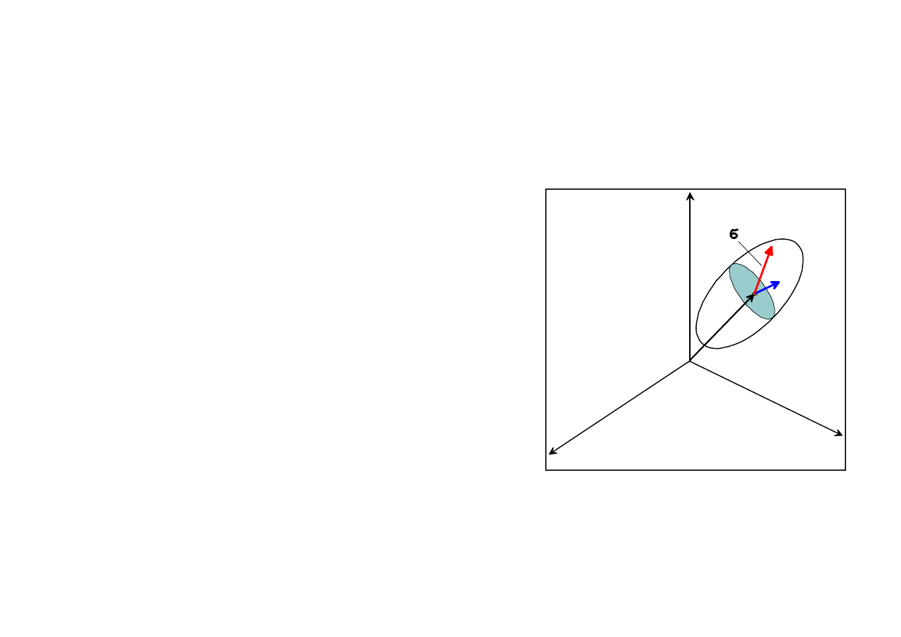
According to

Cauchy hypothesis

, the surface (or interface) reaction force acting between

two adjacent portions of a fluid can be characterized by its surface vector density called the
stress.

Thus, for an infinitesimal piece

dA

of the interface

1

2







 

, we have (see figure)

d

dA



F

σ

and

2

1

1

2

dA



















F

σ

The stress vector

σ

is not a vector field: it depends not

only on the point

x

but also on the orientation of the

surface element

dA

or – equivalently – on the vector

n

normal (perpendicular) to

dA

at the point

x

.

From the 3

rd

principle of Newton’s dynamics (action-reaction principle) we have

( , )

( ,

)

 



σ x n

σ x n

x

1

x

3

x

2

0









dA

n

dF = dA

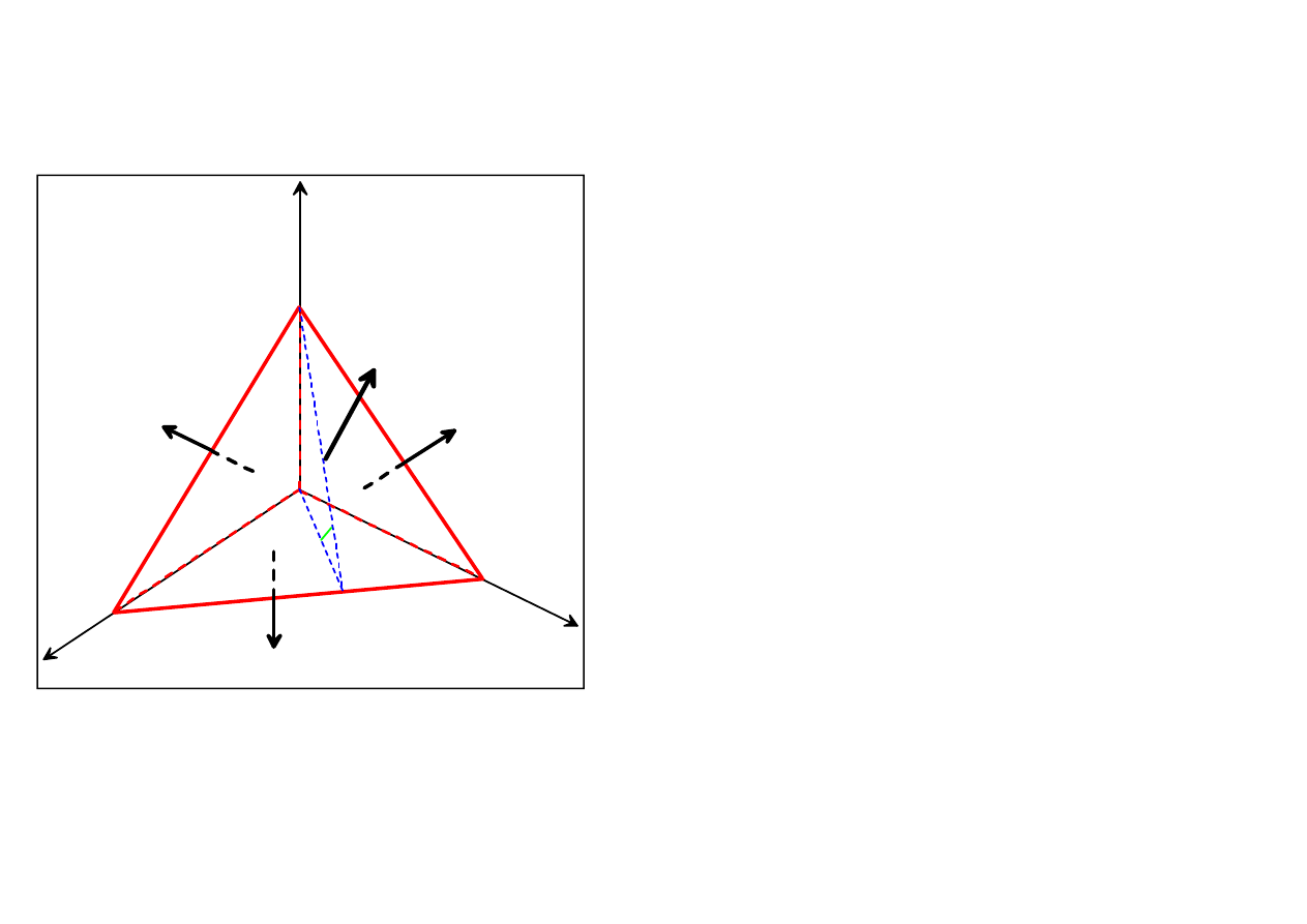
We will show that the value of stress vector

σ

can be expressed by means of a tensor field. To

this aim, consider a portion of fluid in the form of small tetrahedron as depicted in the figure
below.

The front face

ABC



belongs to the plane which

is describes by the following formula

j

j

( , )

n x

h





n x

,

h

– small number.

The areas of the faces of the tetrahedron are S, S

1

,

S

2

and S

3

for

ABC



,

OBC



,

AOC



and

ABO



, respectively. Obviously,

2

S

O(h )



.

Moreover, the following relations hold for
j = 1,2,3:

j

j

j

j

S

Scos[ ( , )] S ( , ) Sn



 



n e

n e



The volume of the tetrahedron is

3

V

O(h )





.

x

1

x

3

x

2

0



n=[n

1

,n

2

,n

3

]

-e

1

-e

2

-e

3

A

B

C

D

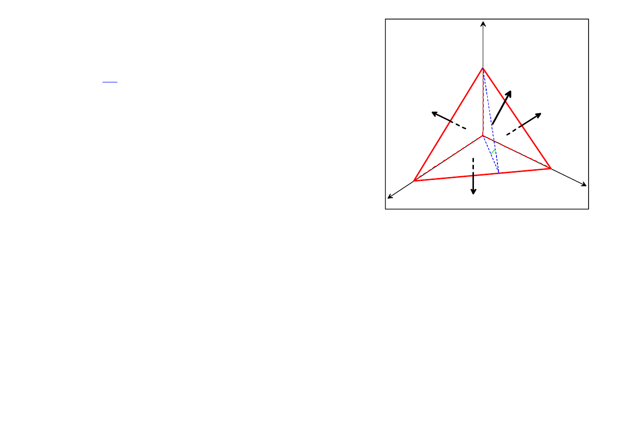
The momentum principle for the fluid contained inside
the tetrahedron volume reads





time derivative

of the momentum

total surface

total volume

fo

vol

surf

rce

force

d

d

dt











v x

F

F



We need to calculate the total surface force

surf

F

.

We have:

on

ABC



:

( , )

( , ) O(h)





σ x n

σ 0 n

ABC

3

surf

S ( , ) O(h )







F

σ 0 n

on

OBC



:

1

1

1

( ,

)

( , )

( , ) O(h)



 

 



σ x e

σ x e

σ 0 e

OBC

3

3

1

1

1

1

surf

S

( , ) O(h )

Sn

( , ) O(h )



 



 



F

σ 0 e

σ 0 e

on

AOC



:

2

2

2

( ,

)

( ,

)

( ,

) O(h)



 

 



σ x e

σ x e

σ 0 e

AOC

3

3

2

2

2

2

surf

S

( ,

) O(h )

Sn

( ,

) O(h )



 



 



F

σ 0 e

σ 0 e

on

AOB



:

3

3

3

( ,

)

( ,

)

( ,

) O(h)



 

 



σ x e

σ x e

σ 0 e

AOB

3

3

3

3

3

3

surf

S

( ,

) O(h )

Sn

( ,

) O(h )



 



 



F

σ 0 e

σ 0 e

x

1

x

3

x

2

0



n=[n

1

,n

2

,n

3

]

-e

1

-e

2

-e

3

A

B

C

D

When the above formulas are inserted to the equation of motion we get



3

2

3

O( h )

O(h )

O( h )

3

vol

j

j

d

d

S[ ( , ) n

( , ) ] O(h )

dt















v x

F

σ 0 n

σ 0 e









When

h

0



the above equation reduces to

j

j

( , ) n

( , )

0





σ 0 n

σ 0 e

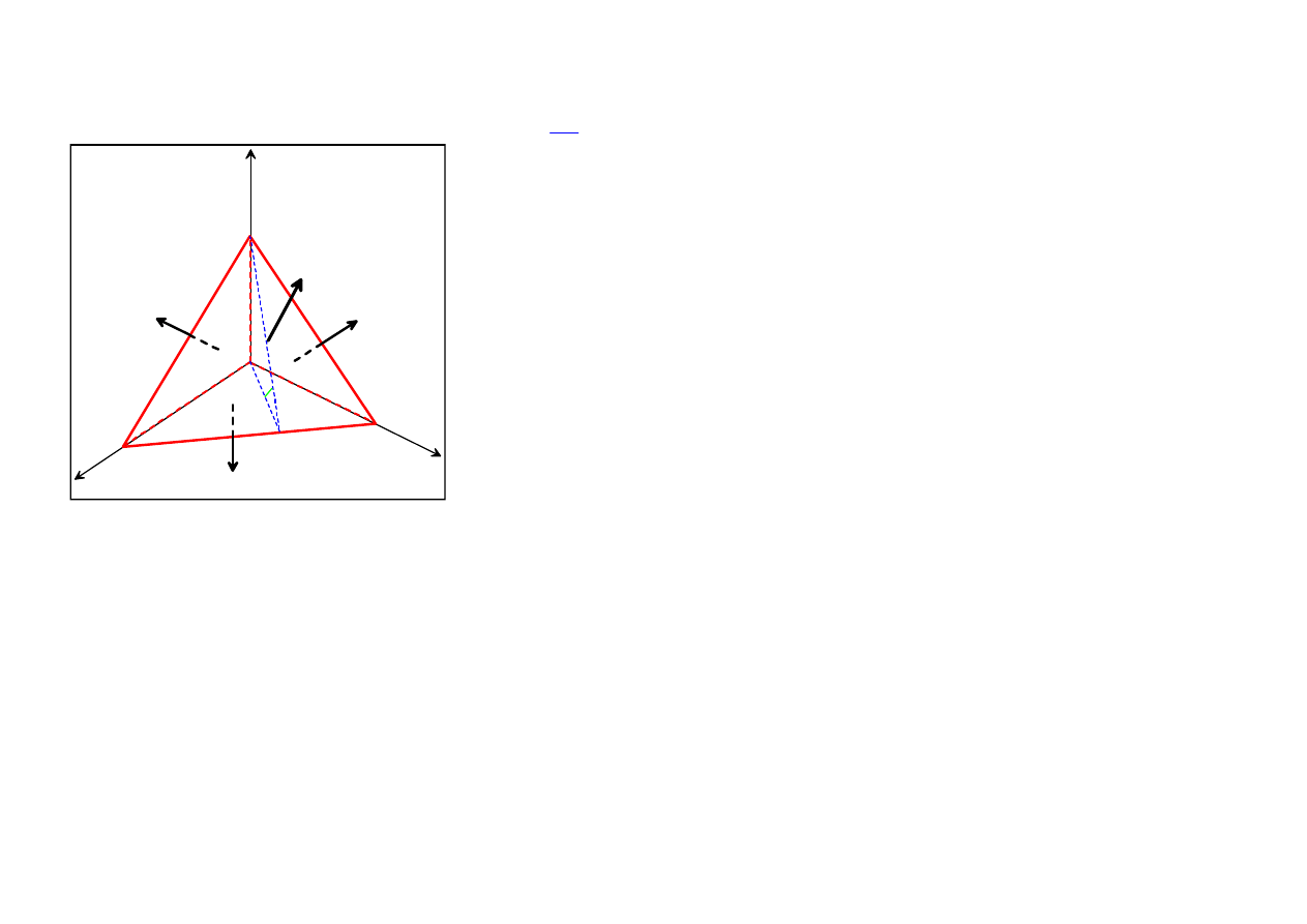
In general case, the vertex O is not the origin of the coordinate
system and the field of stress is time dependent. Hence, we
can write

j

j

(t, , )

n

(t, , )



σ

x n

σ

x e

In the planes oriented perpendicularly to the vectors

e

1

,

e

2

or

e

3

,

the stress vector can be

written as

j

ij

i

(t, , )

(t, )





σ

x e

x e

Thus, the general formula for the stress vector takes the form

j

j

ij

j i

(t, , ) n

(t, , )

(t, )n

(t, )









σ

x n

σ

x e

x

e

Ξ

x n

We have introduced the matrix

Ξ

which represents the stress tensor. The stress tensor

depends on time and space coordinates, i.e., we actually have the tensor field.

x

1

x

3

x

2

0



n=[n

1

,n

2

,n

3

]

-e

1

-e

2

-e

3

A

B

C

D

Note that the stress tensor



can be viewed as the linear mapping (parameterized by

t

and

x

)

between vectors in 3-dimensional Euclidean space

3

3

j j

ij

j i

: E

w

w

E











w

e

e



In particular

ij

j i

( )

n











n

Ξn

e

σ

i.e., the action of



on the normal vector

n

at some point of the fluid surface yields the

stress vector

σ

at this point.

It is often necessary to calculate the normal and tangent stress components at the point of
some surface.

Normal component is equal

inner (scal

n

ar)

product

(

)

( ,

)







n

σ

n Σn n

n Σn





Tangent component can be expressed as

 

i

n

m

m

ij

j i

km k

i i

ij

j

km k

i

i

n

(

n n )n

[

n

(

n n )n ]

 









σ

σ

σ

n

e

e

e

















or, equivalently (verify!) as

(

)

 



σ

n

σ n



C

C

O

O

N

N

S

S

T

T

I

I

T

T

U

U

T

T

I

I

V

V

E

E

R

R

E

E

L

L

A

A

T

T

I

I

O

O

N

N

The constitutive relation for the (simple) fluids is the relation between stress tensor

Ξ

and

the deformation rate tensor

D

. This relation should be postulated in a form which is frame-

invariant and such that the stress tensor is symmetric.

Let’s remind two facts:

 The velocity gradient

v

can be decomposed into two parts: the symmetric part

D

called the deformation rate tensor and the skew-symmetric part

R

called the (rigid)

rotation tensor.

 



v

D R

 Tensor

D

can be expressed as the sum of the spherical part

D

SPH

and the deviatoric part

D

DEV

DEV

SPH





D

D

D

where

SPH

tr

1

1

(

)

3

3



 

 

D

D

I

v I

and

j

i

k

DEV

DEV ij

ij

j

i

k

v

v

v

1

1

1

div

(

)

3

2

x

x

3 x





























 













D

D

v I

D

The general constitutive relation for a (simple) fluid can be written in the form of the matrix
“polynomial”

2

3

0

0

1

2

3

( )

c

c

c

c

...















Ξ

D

Σ

I

D

D

D

P

where the coefficients are the function of 3 invariants of the tensor

D

, i.e.

1

2

3

k

k

c

c [ I ( ),I ( ),I ( )]



D

D

D

.

Consider the characteristic polynomial of the tensor

D

3

2

1

2

3

p ( )

det[

]

I

I

I















 







D

D

I

.

The Cayley-Hamilton Theorem states that the matrix (or tensor) satisfies its own
characteristic polynomial meaning that

3

2

1

2

3

p ( )

I

I

I

 









D

D

D

D

D

0

Thus, the 3

rd

power of

D

(and automatically all higher powers) can be expressed as a linear

combinations of

I

,

D

and

D

2

.

Hence, the most general polynomial constitutive relation is given by the 2

nd

order formula

2

0

0

1

2

( )

c

c

c











Σ

D

Σ

I

D

D

P

N

N

E

E

W

W

T

T

O

O

N

N

I

I

A

A

N

N

F

F

L

L

U

U

I

I

D

D

S

S

The behavior of many fluids (water, air, others) can be described quite accurately by the
linear constitutive relation. Such fluids are called

Newtonian fluids

.

For Newtonian fluids we assume that:



0

c

is a linear function of the invariant

I

1

,



1

c

is a constant,



2

c

0



.

If there is no motion we have the Pascal Law: pressure in any direction is the same. It means
that the matrix

0

Ξ

should correspond to a spherical tensor and

0

0

p

p

 

 



n

I

Ξ

Ξ

The constitutive relation for the Newtonian fluids can be written as follows









1

1

0

0

0

I ( )

2

DEV

c

c

3

p

(

)

2

p

(

)(

)

2











 

 





 









D

Ξ

Ξ

v

Ξ

I

I

D

I

v I

D





where



μ

- (shear) viscosity (the physical unit in SI is kg/m∙s)



ζ

- bulk viscosity (the same unit as

μ

) ; usually

  

and

can be assumed zero

.

The constitutive relation can be written in the index notation

j

k

i

2

3

ij

ij

k

j

i

v

v

v

p (

)

x

x

x

















































  













For an incompressible fluid we have

j

j

v

div

0

x



  







v

v

and the constitutive relation

reduces to the simpler form

p

2



 



Ξ

I

D

or, in the index notation

ij

ij

i

j

j

i

p

v

v

x

x



























 









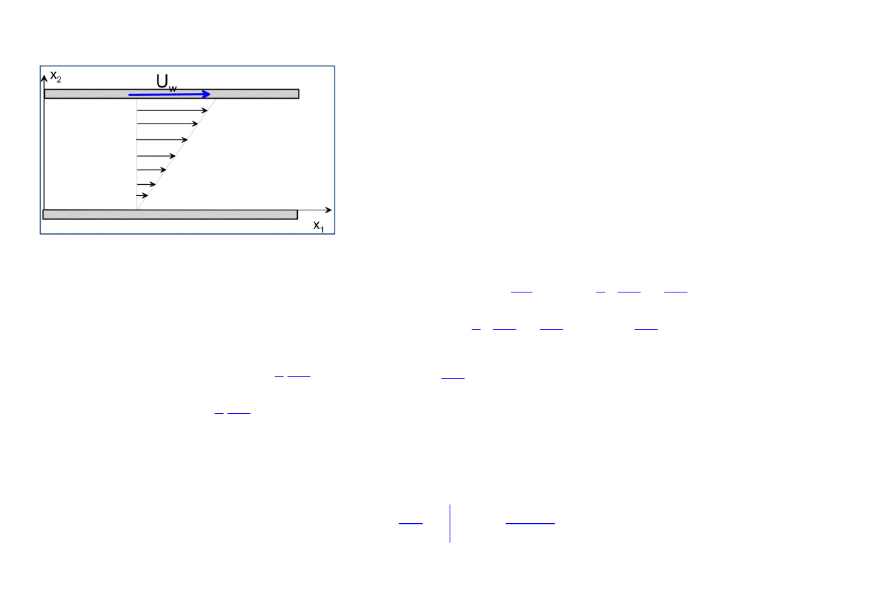
Example: Calculate the tangent stress in the wall shear layer.

The velocity field is defined as follows:

1

1

2

2

2

1

2

v ( ,

)

/

,

v ( ,

)

0

wall

x x

U

x

H

x x





and the pressure is constant. At the bottom wall, the
normal vector which points outwards is

[0, 1]





n

.

Then



1

1

2

1

2

1

1

2

2

2

1

2

1

1

2

2

1

2

v

v

v

1

x

2

x

x

v

v

v

1

[0, 1]

2

x

x

x

v

v

1
2 x

w

x

v

1
2 x

(

)

0

0

p

2

2

(

)

p

1

0

0

0

U / H

2

0

p

1

p

p

























































 







 













 









 





















 

























 











 

















σ

Ξn

n

Dn

According to the action-reaction principle, the tangent stress at the bottom wall is

2

1

v

w

wall

x

wall

U

H













