s1
s2
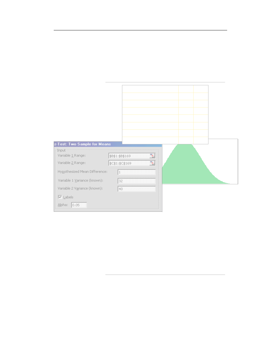
Mean
7.3202
7.2345
Variance
32.6754 40.1309
Observations
168
168
Df
167
167
0.8142
P (F< = f) one–tail
0.0926
F Critical one–tail
0.8747
Statistical
Analysis with
Excel
Excel for Professionals
2002 VJ Books. All rights reside with the author.

Statistical Analysis with Excel
2
S
S
S
t
t
t
a
a
a
t
t
t
i
i
i
s
s
s
t
t
t
i
i
i
c
c
c
a
a
a
l
l
l
A
A
A
n
n
n
a
a
a
l
l
l
y
y
y
s
s
s
i
i
i
s
s
s
W
W
W
i
i
i
t
t
t
h
h
h
E
E
E
x
x
x
c
c
c
e
e
e
l
l
l
Volume 5 in the series
E
E
E
x
x
x
c
c
c
e
e
e
l
l
l
f
f
f
o
o
o
r
r
r
P
P
P
r
r
r
o
o
o
f
f
f
e
e
e
s
s
s
s
s
s
i
i
i
o
o
o
n
n
n
a
a
a
l
l
l
s
s
s
Volume 1: Excel For Beginners
Volume 2: Charting in Excel
Volume 3: Excel-- Beyond The Basics
Volume 4: Managing & Tabulating Data in Excel
Volume 5: Statistical Analysis with Excel
Volume 6: Financial Analysis using Excel
Published by VJ
Books Inc
All rights reserved. No part of this book may be used or reproduced in any form or by
any means, or stored in a database or retrieval system, without prior written
permission of the publisher except in the case of brief quotations embodied in
reviews, articles, and research papers. Making copies of any part of this book for any
purpose other than personal use is a violation of United States and international
copyright laws.
First year of printing: 2002
Date of this copy: Saturday, December 14, 2002
This book is sold as is, without warranty of any kind, either express or implied,
respecting the contents of this book, including but not limited to implied warranties
for the book's quality, performance, merchantability, or fitness for any particular
purpose. Neither the author, the publisher and its dealers, nor distributors shall be
liable to the purchaser or any other person or entity with respect to any liability, loss,
or damage caused or alleged to be caused directly or indirectly by the book.
This book is based on Excel versions 97 to XP. Excel, Microsoft Office, Microsoft
Word, and Microsoft Access are registered trademarks of Microsoft Corporation.
Publisher: VJ
Books Inc, Canada
Author: Vijay Gupta

3
ABOUT THE AUTHOR
Vijay Gupta has taught statistic, econometrics, and finance to institutions in
the US and abroad, specializing in teaching technical material to
professionals.
He has organized and held training workshops in the Middle East, Africa,
India, and the US. The clients include government agencies, financial
regulatory bodies, non-profit and private sector companies.
A Georgetown University graduate with a Masters degree in economics, he
has a vision of making the tools of econometrics and statistics easily
accessible to professionals and graduate students. His books on SPSS and
Regression Analysis have received rave reviews for making statistics and
SPSS so easy and “non-mathematical.” The books are in use by over 150,000
users in more than 140 nations.
He is a member of the American Statistics Association and the Society for
Risk Analysis.
In addition, he has assisted the World Bank and other organizations with
econometric analysis, survey design, design of international investments,
cost-benefit, and sensitivity analysis, development of risk management
strategies, database development, information system design and
implementation, and training and troubleshooting in several areas.
Vijay has worked on capital markets, labor policy design, oil research, trade,
currency markets, and other topics.

Statistical Analysis with Excel
4
V
V
V
I
I
I
S
S
S
I
I
I
O
O
O
N
N
N
Vijay has a vision for software tools for Office Productivity and
Statistics. The current book is one of the first tools in stage one of his
vision. We now list the stages in his vision.
Stage one: Books to Teach Existing Software
He is currently working on books on word-processing, and report
production using Microsoft Word, and a booklet on Professional
Presentations.
The writing of the books is the first stage envisaged by Vijay for
improving efficiency and productivity across the world. This directly
leads to the second stage of his vision for productivity improvement
in offices worldwide.
Stage two: Improving on Existing Software
The next stage is the construction of software that will radically
improve the usability of current Office software.
Vijay’s first software is undergoing testing prior to its release in Jan
2003. The software — titled “Word Usability Enhancer” — will
revolutionize the way users interact with Microsoft Word, providing
users with a more intuitive interface, readily accessible tutorials, and
numerous timesaving and annoyance-removing macros and utilities.
He plans to create a similar tool for Microsoft Excel, and, depending
on resource constraints and demand, for PowerPoint, Star Office, etc.

5
Stage 3: Construction of the first “feedback-designed” Office and Statistics
software
Vijay’s eventual goal is the construction of productivity software
that will provide stiff competition to Microsoft Office. His hope is
that the success of the software tools and the books will convince
financiers to provide enough capital so that a successful software
development and marketing endeavor can take a chunk of the multi-
billion dollar Office Suite market.
Prior to the construction of the Office software, Vijay plans to
construct the “Definitive” statistics software. Years of working on
and teaching the current statistical software has made Vijay a
master at picking out the weaknesses, limitations, annoyances, and,
sometimes, pure inaccessibility of existing software. This 1.5 billion
dollar market needs a new visionary tool, one that is appealing and
inviting to users, and not forbidding, as are several of the current
software. Mr. Gupta wants to create integrated software that will
encompass the features of SPSS, STATA, LIMDEP, EViews,
STATISTICA, MINITAB, etc.
Other
He has plans for writing books on the “learning process.” The books
will teach how to understand one’s approach to problem solving and
learning and provide methods for learning new techniques for self-
learning.

CONTENTS
C H A P T E R 1
WRITING FORMULAS 25
1.1
The Basics Of Writing Formulae 26
1.2
Tool for using this chapter effectively: Viewing the formula instead of the end
result 26
1.2.a
The “A1” vs. the “R1C1“ style of cell references 28
1.2.b
Writing a simple formula that references cells 29
1.3
Types Of References Allowed In A Formula 30
1.3.a
Referencing cells from another worksheet 30
1.3.b
Referencing a block of cells 30
1.3.c
Referencing non–adjacent cells 31
1.3.d
Referencing entire rows 32
1.3.e
Referencing entire columns 32
1.3.f
Referencing corresponding blocks of cells/rows/columns from a set of
worksheets 33
C H A P T E R 2
COPYING/CUTTING AND PASTING FORMULAE 35
2.1
Copying And Pasting A Formula To Other Cells In The Same Column 36
2.2
Copying And Pasting A Formula To Other Cells In The Same Row 37
2.3
Copying And Pasting A Formula To Other Cells In A Different Row And Column
38
2.4
Controlling Cell Reference Behavior When Copying And Pasting Formulae (Use
Of The “$” Key) 39
2.4.a
Using the “$” sign in different permutations and computations in a
formula 41
2.5
Copying And Pasting Formulas From One Worksheet To Another 42
2.6
Pasting One Formula To Many Cells, Columns, Rows 43
2.7
Pasting Several Formulas To A Symmetric But Larger Range 43
2.8
Defining And Referencing A “Named Range” 43
Adding several named ranges in one step 46
Using a named range 47
2.9
Selecting All Cells With Formulas That Evaluate To A Similar Number Type 48
2.10
Special Paste Options 48
2.10.a
Pasting only the formula (but not the formatting and comments) 48
2.10.b
Pasting the result of a formula, but not the formula itself 48
2.11
Cutting And Pasting Formulae 49

Intoduction & Contents
7
2.11.a
The difference between “copying and pasting” formulas and “cutting and
pasting” formulas 49
2.12
Creating A Table Of Formulas Using Data/Table 50
2.13
Saving Time By Writing, Copying And Pasting Formulas On Several Worksheets
Simultaneously 50
C H A P T E R 3
PASTE SPECIAL 52
3.1
Pasting The Result Of A Formula, But Not The Formula 53
3.2
Other Selective Pasting Options 56
3.2.a
Pasting only the formula (but not the formatting and comments) 56
3.2.b
Pasting only formats 56
3.2.c
Pasting data validation schemes 57
3.2.d
Pasting all but the borders 57
3.2.e
Pasting comments only 57
3.3
Performing An Algebraic “Operation” When Pasting One Column/Row/Range On
To Another 58
3.3.a
Multiplying/dividing/subtracting/adding all cells in a range by a number
58
3.3.b
Multiplying/dividing the cell values in cells in several “pasted on”
columns with the values of the copied range 59
3.4
Switching Rows To Columns 59
C H A P T E R 4
INSERTING FUNCTIONS 61
4.1
Basics 61
4.2
A Simple Function 64
4.3
Functions That Need Multiple Range References 67
4.4
Writing A “Function Within A Function” 69
4.5
New Function-Related Features In The XP Version Of Excel 73
Searching for a function 73
4.5.a
Enhanced Formula Bar 73
4.5.b
Error Checking and Debugging 74
C H A P T E R 5
TRACING CELL REFERENCES & DEBUGGING FORMULA
ERRORS 76
5.1
Tracing the cell references used in a formula 76
5.2
Tracing the formulas in which a particular cell is referenced 78
5.3
The Auditing Toolbar 79
5.4
Watch window (only available in the XP version of Excel) 80

Statistical Analysis with Excel
8
5.5
Error checking and Formula Evaluator (only available in the XP version of Excel)
81
5.6
Formula Auditing Mode (only available in the XP version of Excel) 84
5.7
Cell-specific Error Checking and Debugging 85
5.8
Error Checking Options 86
C H A P T E R 6
FUNCTIONS FOR BASIC STATISTICS 89
6.1
“Averaged” Measures Of Central Tendency 90
6.1.a
AVERAGE 90
6.1.b
TRIMMEAN (“Trimmed mean”) 91
6.1.c
HARMEAN (“Harmonic mean”) 92
6.1.d
GEOMEAN (“Geometric mean”) 93
6.2
Location Measures Of Central Tendency (Mode, Median) 94
6.2.a
MEDIAN 95
6.2.b
MODE 95
6.3
Other Location Parameters (Maximum, Percentiles, Quartiles, Other) 95
6.3.a
QUARTILE 96
6.3.b
PERCENTILE 96
6.3.c
Maximum, Minimum and “Kth Largest” 97
MAX (“Maximum value”) 97
MIN (“Minimum value”) 98
LARGE 98
SMALL 99
6.3.d
Rank or relative standing of each cell within the range of a series 99
PERCENTRANK 99
RANK 100
6.4
Measures Of Dispersion (Standard Deviation & Variance) 100
Sample dispersion: STDEV, VAR 100
Population dispersion: STDEVP, VARP 101
6.5
Shape Attributes Of The Density Function (Skewness, Kurtosis) 102
6.5.a
Skewness 102
6.5.b
Kurtosis 104
6.6
Functions Ending With An “A” Suffix 105
C H A P T E R 7
PROBABILITY DENSITY FUNCTIONS AND CONFIDENCE
INTERVALS 109
7.1
Probability Density Functions (PDF), Cumulative Density Functions (CDF), and
Inverse functions 110
7.1.a
Probability Density Function (PDF) 110
7.1.b
Cumulative Density Function (CDF) 111
The CDF and Confidence Intervals 112
7.1.c
Inverse mapping functions 114

Intoduction & Contents
9
7.2
Normal Density Function 115
Symmetry 116
Convenience of using the Normal Density Function 117
Are all large-sample series Normally Distributed? 117
Statistics & Econometrics: Dependence of Methodologies on the assumption
of Normality 118
The Standard Normal and its power 119
7.2.a
The Probability Density Function (PDF) and Cumulative Density Function
(CDF) 119
7.2.b
Inverse function 121
7.2.c
Confidence Intervals 121
95% Confidence Interval 121
90% Confidence Interval 122
7.3
Standard Normal or Z–Density Function 123
Inverse function 124
Confidence Intervals 124
7.4
T–Density Function 125
Inverse function 126
Confidence Intervals 126
7.4.a
One–tailed Confidence Intervals 127
95% Confidence Interval 127
90% Confidence Interval 127
7.5
F–Density Function 129
Inverse function 129
One–tailed Confidence Intervals 130
7.6
Chi-Square Density Function 130
Inverse function 131
One–tailed Confidence Intervals 131
7.7
Other Continuous Density Functions: Beta, Gamma, Exponential, Poisson,
Weibull & Fisher 132
7.7.a
Beta Density Function 132
Inverse Function 133
Confidence Intervals 134
7.7.b
Gamma Density Function 134
Inverse Function 135
Confidence Intervals 136
7.7.c
Exponential Density Function 136
7.7.d
Fisher Density Function 138
7.7.e
Poisson Density Function 138
7.7.f
Weibull Density Function 138
7.7.g
Discrete probabilities— Binomial, Hypergeometric & Negative Binomial
139
Binomial Density Function 139
Hypergeometric Density Function 139
Negative Binomial 139
7.8
List of Density Function 140
7.9
Some Inverse Function 141

Statistical Analysis with Excel
10
C H A P T E R 8
OTHER MATHEMATICS & STATISTICS FUNCTIONS 144
8.1
Counting and summing 145
COUNT function 145
COUNTA function also counts cells with logical or text values 147
COUNTBLANK function counts the number of empty cells in the range
reference 148
SUM function 148
PRODUCT function 149
SUMPRODUCT function 149
8.2
The “If” counting and summing functions: Statistical functions with logical
conditions 150
SUMIF function 150
COUNTIF function 151
8.3
Transformations (log, exponential, absolute, sum, etc) 153
Standardizing a series that follows a Normal Density Function 155
8.4
Deviations from the Mean 156
DEVSQ 156
AVEDEV 156
8.5
Cross series relations 157
8.5.a
Covariance and correlation functions 157
8.5.b
Sum of Squares 157
SUMXMY2 function 158
SUMX2MY2 function 158
C H A P T E R 9
ADD-INS: ENHANCING EXCEL 161
9.1
Add-Ins: Introduction 161
9.1.a
What can an Add-In do? 162
9.1.b
Why use an Add-In? 162
9.2
Add–ins installed with Excel 162
9.3
Other Add-Ins 163
9.4
The Statistics Add-In 163
9.4.a
Choosing the Add-Ins 163
C H A P T E R 1 0
STATISTICS TOOLS 169
10.1
Descriptive statistics 170
10.2
Rank and Percentile 175
Interpreting the output: 177
10.3
Bivariate relations— correlation, covariance 178
Correlation analysis 178
Interpreting the output 179
10.3.a
Covariance tool and formula 180

Intoduction & Contents
11
C H A P T E R 1 1
HYPOTHESIS TESTING 183
11.1
Z-testing for population means when population variances are known 184
Interpreting the output 189
11.2
T-testing means when the two samples are from distinct groups 189
11.2.a
The pretest— F-testing for equality in variances 189
Interpreting the output 191
11.2.b
T-test: Two–Sample Assuming Unequal Variances 193
Interpreting the output 196
11.2.c
T-test: Two–Sample Assuming Equal Variances 199
11.3
Paired Sample T-tests 199
11.4
ANOVA 205
Interpreting the output 207
C H A P T E R 1 2
REGRESSION 211
12.1
Assumptions Underlying Regression Models 211
12.1.a
Assumption 1: The relationship between any one independent series and
the dependent series can be captured by a straight line in a 2–axis graph
213
12.1.b
Assumption 2: The independent variables do not change if the sampling is
replicated 213
12.1.c
Assumption 3: The sample size must be greater than the number of
independent variables (N should be greater than K–1) 214
12.1.d
Assumption 4: Not all the values of any one independent series can be the
same 215
12.1.e
Assumption 5: The residual or disturbance error terms follow several rules
216
Assumption 5a:
The mean/average or expected value of the disturbance
equals zero 216
Assumption 5b:
The disturbance terms all have the same variance 216
Assumption 5c:
A disturbance term for one observation should have no
relation with the disturbance terms for other observations or with any
of the independent variables 217
Assumption 5d:
There is no specification bias 217
Assumption 5e:
The disturbance terms have a Normal Density Function 218
12.1.f
Assumption 6: There are no strong linear relationships among the
independent variables 218
12.2
Conducting the Regression 219
12.3
Brief guideline for interpreting regression output 222
12.4
Breakdown of classical assumptions: validation and correction 226
C H A P T E R 1 3
OTHER TOOLS FOR STATISTICS 229
13.1
Sampling analysis 229
13.2
Random Number Generation 231

Statistical Analysis with Excel
12
13.3
Time series 234
Exponential Smoothing 234
Moving Average analysis 235
C H A P T E R 1 4
THE SOLVER TOOL FOR CONSTRAINED LINEAR OPTIMIZATION
239
14.1
Defining the objective function (Choosing the optimization criterion) 239
14.2
Adding constraints 243
14.3
Choosing Algorithm Options 244
Running the Solver 245
INDEX 245

Intoduction & Contents
13
Mapping of menu options with sections of the book
and in the series of books
You may be looking for a section that pertains to a particular menu option
in Excel. I now briefly lay out where to find (in the series) a discussion of
a specific menu option of Excel.
Table 1: Mapping of the options in the “FILE“ menu
Menu Option
Section that discusses the option
OPEN
SAVE
SAVE AS
Volume 1: Excel For Beginners
Volume 4: Managing & Tabulating Data in Excel
SAVE AS WEB PAGE
Volume 1: Excel For Beginners
Volume 4: Managing & Tabulating Data in Excel
SAVE WORKSPACE
Volume 4: Managing & Tabulating Data in Excel
SEARCH
Volume 1: Excel For Beginners
PAGE SETUP
Volume 1: Excel For Beginners
PRINT AREA
Volume 1: Excel For Beginners
PRINT PREVIEW
Volume 1: Excel For Beginners
Volume 1: Excel For Beginners
PROPERTIES
Volume 1: Excel For Beginners
Table 2: Mapping of the options in the “EDIT“ menu
Menu Option
Section that discusses the option
UNDO
Volume 1: Excel For Beginners
REDO
Volume 1: Excel For Beginners
CUT
COPY
Various

Statistical Analysis with Excel
14
Menu Option
Section that discusses the option
PASTE
OFFICE CLIPBOARD
Volume 1: Excel For Beginners
PASTE SPECIAL
Volume 3: Excel– Beyond The Basics
FILL
Volume 4: Managing & Tabulating Data in
Excel
CLEAR
Volume 1: Excel For Beginners
DELETE SHEET
Volume 1: Excel For Beginners
MOVE OR COPY SHEET
Volume 1: Excel For Beginners
FIND
Volume 1: Excel For Beginners
REPLACE
Volume 1: Excel For Beginners
GO TO
Volume 3: Excel– Beyond The Basics
LINKS
Volume 3: Excel– Beyond The Basics
OBJECT
Volume 3: Excel– Beyond The Basics
Volume 2: Charting in Excel
Table 3: Mapping of the options in the “VIEW“ menu
Menu Option
Section that discusses the option
NORMAL
Volume 1: Excel For Beginners
PAGE BREAK PREVIEW Volume 1: Excel For Beginners
TASK PANE
Volume 1: Excel For Beginners
TOOLBARS
Volume 1: Excel For Beginners
Volume 3: Excel– Beyond The Basics
FORMULA BAR
Leave it on (checked)
STATUS BAR
Leave it on (checked)
HEADER AND FOOTER Volume 1: Excel For Beginners
COMMENTS
Volume 3: Excel– Beyond The Basics

Intoduction & Contents
15
Menu Option
Section that discusses the option
FULL SCREEN
Volume 1: Excel For Beginners
ZOOM
Volume 1: Excel For Beginners
Table 4: Mapping of the options in the “INSERT“ menu
Menu Option
Section that discusses the option
CELLS
Volume 1: Excel For Beginners
ROWS
Volume 1: Excel For Beginners
COLUMNS
Volume 1: Excel For Beginners
WORKSHEETS
Volume 1: Excel For Beginners
CHARTS
Volume 2: Charting in Excel
PAGE BREAK
Volume 1: Excel For Beginners
FUNCTION
Volume 1: Excel For Beginners
Volume 3: Excel– Beyond The Basics
FUNCTION/FINANCIAL
Volume 6: Financial Analysis using Excel
FUNCTION/STATISTICAL
chapter 6-chapter 8
FUNCTION/LOGICAL
Volume 3: Excel– Beyond The Basics
FUNCTION/TEXT
Volume 3: Excel– Beyond The Basics
FUNCTION/INFORMATION Volume 3: Excel– Beyond The Basics
FUNCTION/LOOKUP
Volume 3: Excel– Beyond The Basics
FUNCTION/MATH & TRIG
Volume 3: Excel– Beyond The Basics
FUNCTION/ENGINEERING section 30.2-section 30.3
FUNCTION/DATABASE
Volume 3: Excel– Beyond The Basics
Volume 4: Managing & Tabulating Data in Excel
FUNCTION/DATE & TIME
Volume 3: Excel– Beyond The Basics
NAME
Volume 1: Excel For Beginners

Statistical Analysis with Excel
16
Menu Option
Section that discusses the option
COMMENT
Volume 3: Excel– Beyond The Basics
PICTURE
Volume 2: Charting in Excel
DIAGRAM
Volume 2: Charting in Excel
OBJECT
Volume 3: Excel– Beyond The Basics
HYPERLINK
Volume 3: Excel– Beyond The Basics
Table 5: Mapping of the options inside the “FORMAT“ menu
Menu Option
Section that discusses the option
CELLS
Volume 1: Excel For Beginners
ROW
Volume 1: Excel For Beginners
COLUMN
Volume 1: Excel For Beginners
SHEET
Volume 1: Excel For Beginners
AUTOFORMAT
Volume 1: Excel For Beginners
CONDITIONAL FORMATTING
Volume 3: Excel– Beyond The Basics
STYLE
Volume 1: Excel For Beginners
Table 6: Mapping of the options inside the “TOOLS“ menu
Menu Option
Section that discusses the option
SPELLING
Volume 1: Excel For Beginners
ERROR CHECKING
Volume 3: Excel– Beyond The Basics
SPEECH
Volume 4: Managing & Tabulating Data in Excel
SHARE WORKBOOK
Volume 3: Excel– Beyond The Basics
TRACK CHANGES
Volume 3: Excel– Beyond The Basics
PROTECTION
Volume 3: Excel– Beyond The Basics

Intoduction & Contents
17
Menu Option
Section that discusses the option
ONLINE COLLABORATION
Volume 3: Excel– Beyond The Basics
GOAL SEEK
Volume 3: Excel– Beyond The Basics
SCENARIOS
Volume 3: Excel– Beyond The Basics
AUDITING
Volume 3: Excel– Beyond The Basics
TOOLS ON THE WEB
The option will take you to a Microsoft site that
provides access to resources for Excel
MACROS
In upcoming book on “Macros for Microsoft Office”
ADD-INS
chapter 9
AUTOCORRECT
Volume 1: Excel For Beginners
CUSTOMIZE
Volume 3: Excel– Beyond The Basics
OPTIONS
Volume 1: Excel For Beginners
Table 7: Mapping of the options inside the “DATA” menu
Menu Option
Section that discusses the option
SORT
Volume 4: Managing & Tabulating Data in Excel
FILTER
Volume 4: Managing & Tabulating Data in Excel
FORM
Volume 4: Managing & Tabulating Data in Excel
SUBTOTALS
Volume 4: Managing & Tabulating Data in Excel
VALIDATION
Volume 4: Managing & Tabulating Data in Excel
TABLE
Volume 1: Excel For Beginners
CONSOLIDATION
section 48.5
GROUP AND OUTLINE Volume 4: Managing & Tabulating Data in Excel
PIVOT REPORT
Volume 4: Managing & Tabulating Data in Excel
EXTERNAL DATA
Volume 4: Managing & Tabulating Data in Excel

Statistical Analysis with Excel
18
Table 8: Mapping of the options inside the “WINDOW“ menu
Menu Option
Section that discusses the option
HIDE
Volume 3: Excel– Beyond The Basics
SPLIT
Volume 1: Excel For Beginners
FREEZE PANES Volume 1: Excel For Beginners
Table 9: Mapping of the options inside the “HELP“ menu
Menu Option
Section that discusses the option
OFFICE ASSISTANT Volume 1: Excel For Beginners
HELP
Volume 1: Excel For Beginners
WHAT’S THIS
Volume 1: Excel For Beginners

Intoduction & Contents
19
INTRODUCTION
Are there not enough Excel books in the market? I have asked myself this
question and concluded that there are books “inside me,” based on what I
have realized from observation by friends, students, and colleagues that I
have a “vision and knack for explaining technical material in plain
English.”
Read the book practicing the lessons on the sample files provided in the
zipped file you downloaded. I hope the book is useful and assists you in
increasing your productivity in Excel usage. You may be pleasantly
surprised at some of the features shown here. They will enable you to
save time.
The “Make me a Guru” series teach technical material in simple English.
A lot of thinking went into the sequencing of chapters and sections. The
book is broken down into logical “functional” components. Chapters are
organized into sections and sub-sections. This creates a smooth flowing
structure, enabling “total immersion” learning. The current book is
broken down into a multi-level hierarchy:
—Chapters, each teaching a specific skill/tool.
— Several sections within each chapter. Each section shows aspect of
the skill/tool taught in the chapter. Each section is numbered—for
example, “Section 1.2” is the numbering for the second section in
chapter 1.
— A few sub-sections (and maybe one further segmentation) within
each section. Each sub-section lists a specific function, task, or
proviso related to the “master” section. The sub-sections are
numbered——for example, “1.2.a” for the first sub-section in the
second section of chapter 1.

Statistical Analysis with Excel
20
Unlike other publishers, I do not consider you dummies or idiots. Each
and everyone had the God given potential to achieve mastery in any field.
All one needs is a guide to show you the way to master a field. I hope to
play this role. I am confident that you will consider your self an Excel
“Guru” (in terms of the typical use of Excel in your profession) and so will
others.
Once you learn the way to master a windows application, this new
approach will enable you to pick up new skills” on the fly.” Do not argue
for your limitations. You have none.
I hope you have a great experience in learning with this book. I would
love feedback. Please use the feedback form on our website vjbooks.net.
In addition, look for updates and sign up for an infrequent newsletter at
the site.
VJ Inc Corporate and Government Training
We provide productivity-enhancement and capacity building for corporate,
government, and other clients. The onsite training includes courses on:
•
Designing and Implementing Improved Information and
Knowledge Management Systems
•
Improving the Co-ordination Between Informational Technology
Departments and Data Analysts & other end-users of
Information
•
Office Productivity Software and Tools
•
Data Mining
•
Financial Analysis

Intoduction & Contents
21
•
Feasibility Studies
•
Risk Analysis, Monitoring and Management
•
Statistics, Forecasting, Econometrics
•
Building and using Credit Rating/Monitoring Models
•
Specific software applications, including Microsoft Excel, VBA,
Word, PowerPoint, Access, Project, SPSS, SAS, STATA, ands
many other
Contact our corporate training group at http://www.vjbooks.net.

Statistical Analysis with Excel
22
STATISTICS PROCEDURES
Three chapters teach statistics functions including the use of Excel
functions for building Confidence Intervals and conducting Hypothesis
Testing for several types of distributions. The design of hypothesis tests
and the intermediate step of demarcating critical regions are taught
lucidly.
It seems that Microsoft has taken pains to “hide” some of the most
powerful tools in Excel. These “hidden” tools are called “Add-Ins.” These
tools work on top of Excel, extending the power and abilities of Excel.
Many Add-Ins are available for specific types of analysis like Risk
Analysis. I show how to use three Add-Ins that install with Excel.
BASICS
The fundamental operations in Excel are taught in Volume 1: Excel For
Beginners, Volume 2: Charting in Excel, and Volume 3: Excel– Beyond The
Basics
FUNCTIONS
I teach the writing of formulas and associated topics in Volume 3: Excel–
Beyond The Basics. I show, in a step-by-step exposition, the proper way
for writing cell references in a formula. The book describe tricks for
copying/cutting and pasting in several examples. In addition, I discuss
special pasting options.
Finally, different types of functions are classified under logical categories
and discussed within the optimal category. The categories include
financial, Statistical, Text, Information, Logical, and “Smart” Logical.

Intoduction & Contents
23
MANAGING & TABULATING DATA
Excel has extremely powerful data entry, data management, and
tabulation tools. The combination of tools provide almost database like
power to Excel. Unfortunately, the poor quality of the menu layout and
the help preclude the possibility of the user self-learning these features.
These features are taught in Volume 4: Managing & Tabulating Data in
Excel
CHARTING
Please refer to book two in this series. The book title is Charting in Excel.
Sample data
Most of the tutorials use publicly available data from the International
labor Organization (ILO). I used a simple data set with only a few
columns and observations. All the sample data files are included in the
zipped file.
The samples for functions use several small data sets that are more suited
to illustrating the power and usefulness of the functions.
I have not included the data set for conducting statistical procedures.
This is intentional; often, readers fail to internalize the few key concepts
of hypothesis testing because they do not subject themselves to a “sink-or-
swim” inference-drawing thinking and imbibing process when
interpreting the results of statistical procedures.

Page for Notes
CHAPTER 1
WRITING FORMULAS
This chapter discusses the following topics:
— THE BASICS OF WRITING FORMULAE
— TOOL FOR USING THIS CHAPTER EFFECTIVELY: VIEWING
THE FORMULA INSTEAD OF THE END RESULT
— The A1 VS THE R1C1 STYLE OF CELL REFERENCES
— TYPES OF REFERENCES ALLOWED IN A FORMULA
— REFERENCING CELLS FROM ANOTHER WORKSHEET
— REFERENCING A BLOCK OF CELLS
— REFERENCING NON–ADJACENT CELLS
— REFERENCING ENTIRE ROWS
— REFERENCING ENTIRE COLUMNS
— REFERENCING CORRESPONDING BLOCKS OF
CELLS/ROWS/COLUMNS FROM A SET OF WORKSHEETS
The most important functionality offered by a spreadsheet application is
the ease and flexibility of writing formulae. In this chapter, I start by
showing how to write simple formula and then build up the level of
complexity of the formulae.
Within the sections of this chapter, you will find tips and notes on
commonly encountered problems or issues in formula writing.

Chapter 1: Writing Formulas
25
1.1
THE BASICS OF WRITING FORMULAE
This section teaches the basics of writing functions.
1.2
TOOL FOR USING THIS CHAPTER EFFECTIVELY:
VIEWING THE FORMULA INSTEAD OF THE END
RESULT
For ease of understanding this chapter, I suggest you use a viewing option
that shows, in each cell on a worksheet, the formula instead of the result.
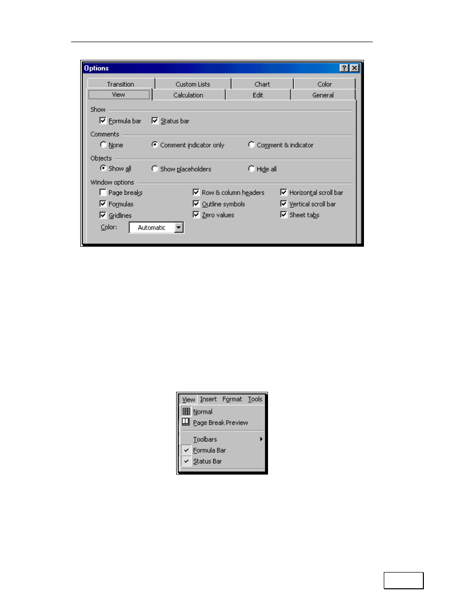
Follow the menu path TOOLS/OPTIONS/VIEW. In the area “Window
Options” select the option “Formulas” as shown in Figure 1.
Execute the dialog by clicking on the button OK. Go back to the
worksheet. The formula will be shown instead of the calculated value.
Eventually you will want to return to the default of seeing the results
instead of the formula. Deselect “formula” in the area “Windows Options”
in TOOLS/OPTIONS/VIEW.
Statistical Analysis with Excel
26
Figure 1: Viewing the formulas instead of the formula result
The effect is only cosmetic; the results will not change. As you shall see
later, what you have just done will facilitate the understanding of
functions.
In addition, leave the option VIEW/ FORMULA BAR selected as shown in
Figure 2.
Figure 2: Select “Formula Bar”

Chapter 1: Writing Formulas
27
1.2.A
THE “A1” VS. THE “R1C1“ STYLE OF CELL REFERENCES
The next figure shows a simple formula. The formula is written into cell
G15. The formula multiplies the values inside cells F8 and F6.
Figure 3: A!-style cell referencing
This style of referencing is called the “A1“ style or “absolute” referencing.
The exact location of the referenced cells is written. (The cells are those
in the 6th and 8th rows of column F.) One typically works with this style.
However, there is another style for referencing the cells in a formula.
This style is called the “R1C1“ style or “relative” referencing. The same
formula as in the previous figure but in R1C1 style is shown in the next
figure.
Figure 4: The same formula as in the previous figure, but in R1C1 (Offset) style cell
referencing while the previous figure showed A1 (Absolute-) style cell referencing
Does not this formula look different? This style uses relative referencing.
So, the first cell (F8) is referenced relative to its position in reference to
the cell that contains the formula (cell G15). Row 8 is 7 rows below row
15 and column F is 1 column before column G. Therefore, the cell
reference is “minus seven rows, minus 1 column” or “R[— 7]C[— 1].”
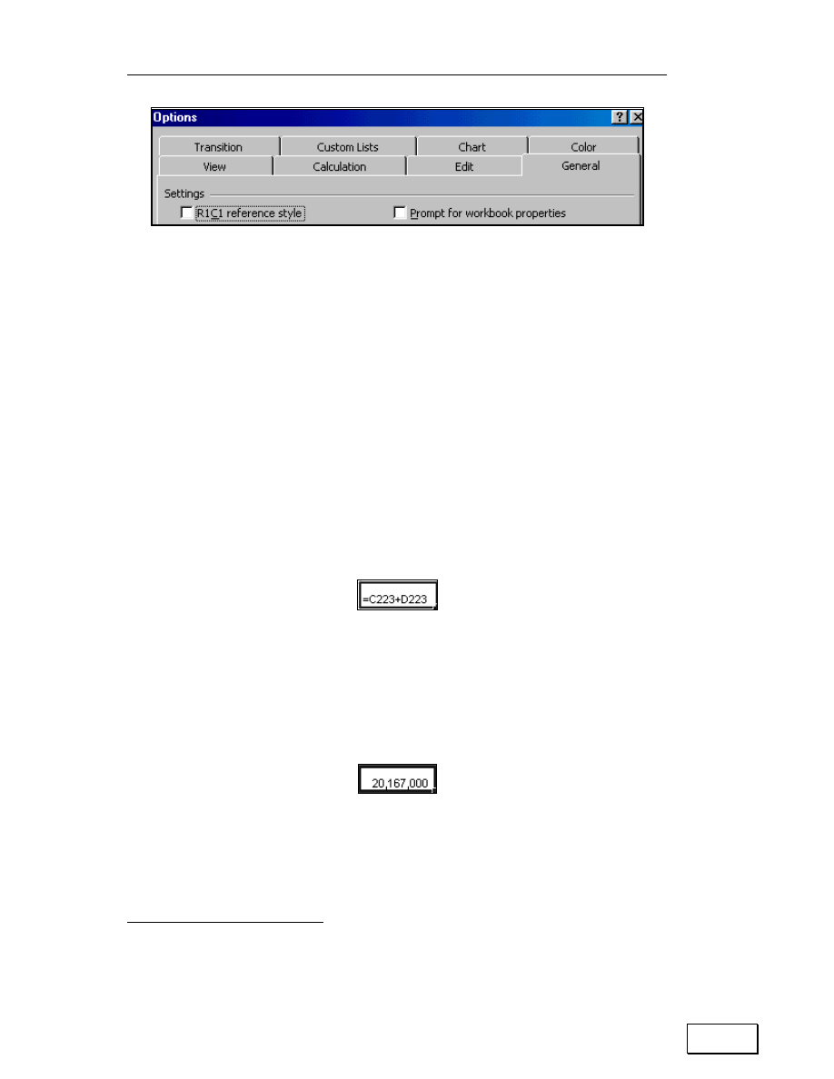
If you see a file or worksheet with such relative referencing, you can
switch all the formulas back to absolute “A1” style referencing by going to
TOOLS/OPTIONS/GENERAL and deselecting the option “R1C1 reference
style.”
Statistical Analysis with Excel
28
Figure 5: Settings for Formula Referencing
1.2.B
WRITING A SIMPLE FORMULA THAT REFERENCES CELLS
Open the sample file “File3.xls” and choose the worksheet “main.”
Assume you want to write add the values in cells C223
1
and D223 (that is,
to calculate “C223 + D223”) and place the result into cell F223.
Click on cell F223. Key-in “=“and then write the formula by clicking on
the cell C223, typing in “+” then clicking on cell “D223.”
Figure 6: Writing a formula
After writing in the formula, press the key ENTER. The cell F223 will
contain the result for the formula contained in it.
Figure 7: The result is shown in the cell on which you wrote the formula
1
Cell C223 is the cell in column C and row 223.

Chapter 1: Writing Formulas
29
1.3
TYPES OF REFERENCES ALLOWED IN A FORMULA
1.3.A
REFERENCING CELLS FROM ANOTHER WORKSHEET
You can reference cells from another worksheet. Choose cell H235 on the
worksheet “main.” In the chosen cell, type the text shown in the next
figure. (Do not press the ENTER key; the formula is incomplete and you
will get an error message if you press ENTER.)
Figure 8: Writing or choosing the reference to the first referenced range
Then select the worksheet “second” and click on cell D235. Now press the
ENTER key. The formula in cell H235 of worksheet “main” references the
cell D235 from the worksheet “second”. The next figure illustrates this.
Figure 9: Writing or choosing the reference to the second referenced range which is not on the
worksheet on which you are writing the formula
In this formula, the part “second!” informs Excel that the range referenced
is from the sheet “second.
1.3.B
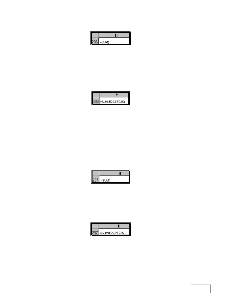
REFERENCING A BLOCK OF CELLS
Select the worksheet “main.” Choose cell H236. In the chosen cell, type
the text shown in the next figure.
Statistical Analysis with Excel
30
Figure 10: This formula requires a block of cells as a reference
Use the mouse to highlight the block of cells “E223 to E235.” Type in a
closing parenthesis and press the ENTER key. The resulting function is
shown in the next figure.
Figure 11: Formula with a block of cells as the reference
1.3.C
REFERENCING NON–ADJACENT CELLS
Choose cell H237. Click in the cell and type the text shown in the next
figure.
Figure 12: The core function is typed first
As in the previous example, choose cells E223 to E235 by highlighting
them— the formula should like the one shown in the next figure.
Figure 13: The first block of cells is referenced
Type a comma. The resulting formula should look like that shown in the
next figure.
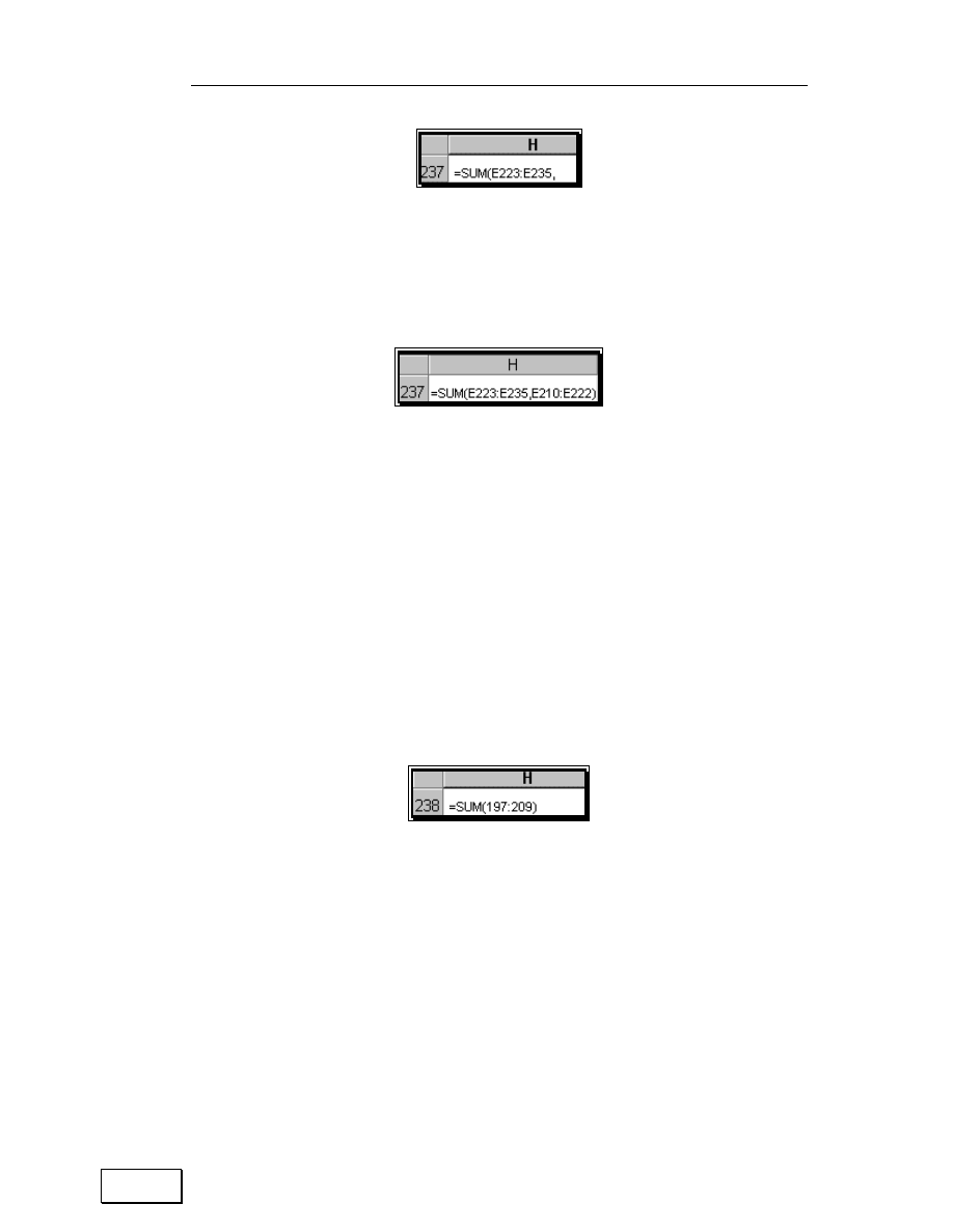
Chapter 1: Writing Formulas
31
Figure 14: Getting the formula ready for the second block of cells
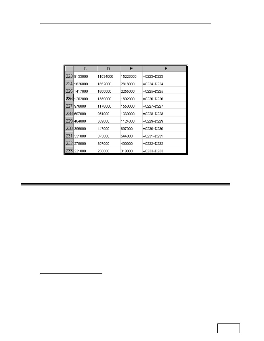
Highlight the block of cells “E210 to E222.” Key-in a closing parenthesis
and press the ENTER key.
Figure 15: The formula with references to two non-adjacent blocks of cells
1.3.D
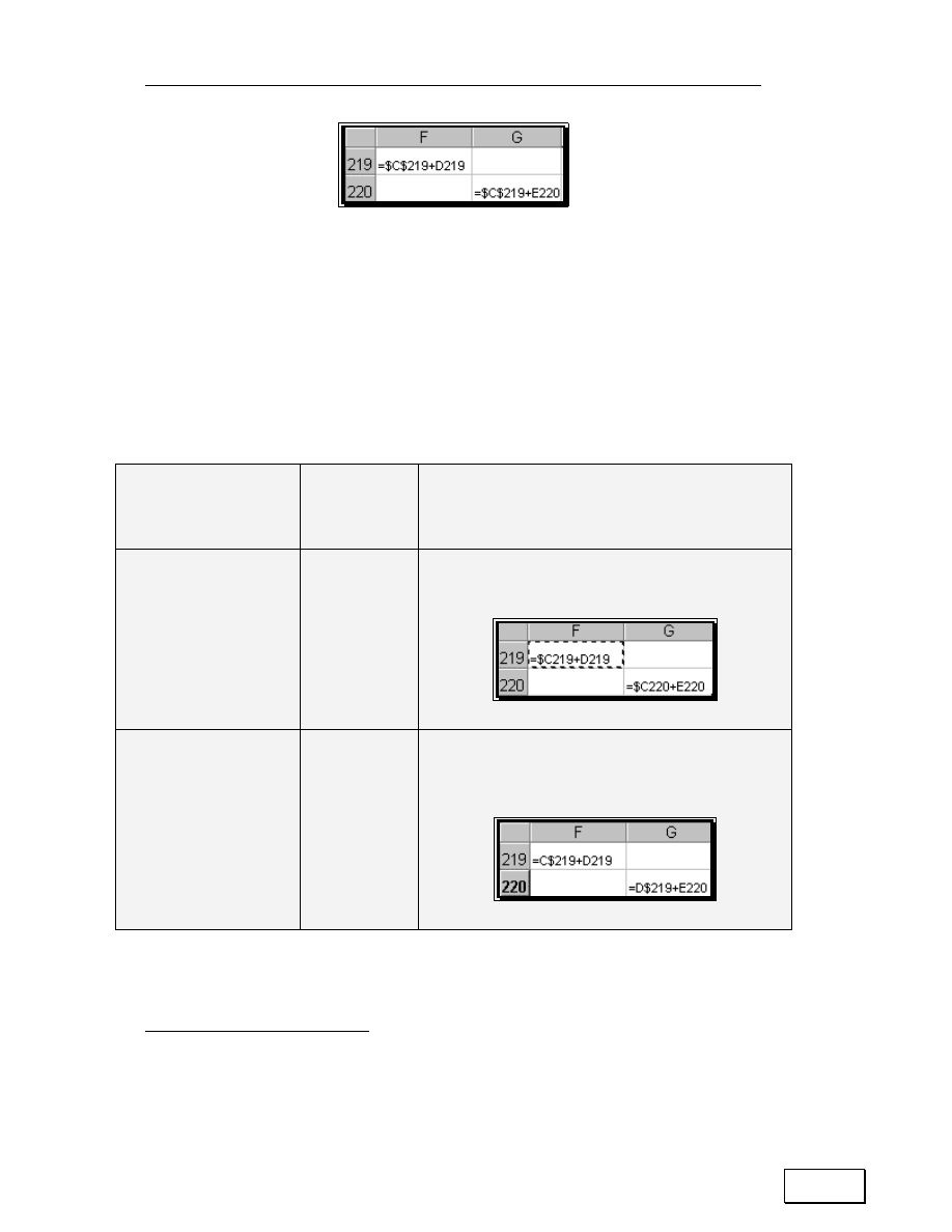
REFERENCING ENTIRE ROWS
Choose cell H238. In this cell, type the text shown in the next figure.
Using the mouse, highlight the rows 197 to 209. Type in a closing
parenthesis and press the ENTER key. The resulting formula is shown in
the next figure.
Figure 16: Referencing entire rows
1.3.E
REFERENCING ENTIRE COLUMNS
Choose cell H239. In this cell, type the text shown in the next figure.
Using the mouse, highlight the columns C and D. Key-in a closing
parenthesis and press the ENTER key.

Statistical Analysis with Excel
32
Figure 17: Referencing entire columns
1.3.F
REFERENCING CORRESPONDING BLOCKS OF
CELLS/ROWS/COLUMNS FROM A SET OF WORKSHEETS
Assume you have a workbook with six worksheets on similar data from
six clients. You want to sum cells “C4 to F56” across all six worksheets.
One way to do this would be to create a formula in each worksheet to sum
for that worksheet’s data and then a formula to add the results of the
other six formulae.
Another way is using “3–D references.” The row and column make the
first two dimensions; the worksheet set is the third dimension. You can
use only one formula that references all six worksheets that the relevant
cells within them.
While typing the formula,
• Type the “=“sign,
• Write the formula (for example, “Sum”),
• Place an opening parenthesis “(,” then
• Select the six worksheets by clicking at the name tab of the first one
and then pressing down SHIFT and clicking on the name tab of the
sixth worksheet, and then
• Highlight the relevant cell range on any one of them,
• Type in the closing parenthesis “)”
• And press the ENTER key to get the formula
=SUM(Sheet1:Sheet6!”C4:F56”)

Page for Notes

Statistical Analysis with Excel
34
CHAPTER 2
COPYING/CUTTING AND
PASTING FORMULAE
This chapter teaches the following topics:
— COPYING AND PASTING A FORMULA TO OTHER CELLS IN
THE SAME COLUMN
— COPYING AND PASTING A FORMULA TO OTHER CELLS IN
THE SAME ROW
— COPYING AND PASTING A FORMULA TO OTHER CELLS IN A
DIFFERENT ROW AND COLUMN
— CONTROLLING CELL REFERENCE BEHAVIOR WHEN
COPYING AND PASTING FORMULAE (USE OF THE “$”
KEY)
— USING THE “$” SIGN IN DIFFERENT PERMUTATIONS AND
COMPUTATIONS IN A FORMULA.
— COPYING AND PASTING FORMULAS FROM ONE
WORKSHEET TO ANOTHER
— SPECIAL PASTE OPTIONS
— PASTING ONLY THE FORMULA (BUT NOT THE FORMATTING
AND COMMENTS)
— PASTING THE RESULT OF A FORMULA, BUT NOT THE
FORMULA ITSELF
— CUTTING AND PASTING FORMULAE
— THE DIFFERENCE BETWEEN “COPYING AND PASTING“
FORMULAS AND “CUTTING AND PASTING” FORMULAS

Chapter 2: Copying/Cutting and pasting formulae
35
— SAVING TIME BY WRITING, COPYING AND PASTING
FORMULAS ON SEVERAL WORKSHEETS
SIMULTANEOUSLY
2.1
COPYING AND PASTING A FORMULA TO OTHER
CELLS IN THE SAME COLUMN
Often one wants to write analogous formulae for several cases. For
example, assume you want to write a formula analogous to the formula in
F223 into each of the cells F224 to F235
2
. The quick way to do this is to:
— Click on the “copied from” cell F223.
— Select the option EDIT/COPY. (The menu can also be accessed by
right-clicking on the mouse or by clicking on the COPY icon.)
— Highlight the “pasted on” cells F224 to F235 and
— Choose the menu option EDIT/PASTE. (The menu can also be
accessed by right-clicking on the mouse or by clicking on the
PASTE icon.)
— Press the ENTER key.
— The formula is pasted onto the cells F224 to F235 and the cell
2
The formula in F223 adds the values in cells that are 3 and 2 columns to the left (that
is, cells in columns in C and D.)
Statistical Analysis with Excel
36
references within each formula are adjusted
3
for the location
difference between the “pasted on” cells and the “copied from” cell.
Figure 18: Pasting a formula
2.2
COPYING AND PASTING A FORMULA TO OTHER
CELLS IN THE SAME ROW
Select the range F223— F235 (which you just created in the previous sub–
section). Select the option EDIT/COPY. Choose the range G223— G235
(that is, one column to the right) and choose the menu option
EDIT/PASTE. Now click on any cell in the range G223— G235 and see
how the column reference has adjusted automatically. The formula in
3
The formula in the “copied cell” F223 is “C223 + D223” while the formula in the
“pasted on” cell F225 is “C225 + D225.” (Click on cell F225 to confirm this.) The cell
F225 is two rows below the cell F223, and the copying-and-pasting process accounts
for that.

Chapter 2: Copying/Cutting and pasting formulae
37
G223 is “D223 + E223” while the formula in F223 was “C223 + D223”.
The next figure illustrates this. Because you pasted one column to the
right, the cell references automatically shifted one column to the right.
So:
— The reference “C” became “D,” and
— The reference “D” became “E.”
Figure 19: Cell reference changes when a formula is copied and pasted
The examples in 2.1 on page 36 and 2.2 on page 37 show the use of “Copy
and Paste” to quickly replicate formula in a manner that maintains
referential parallelism.
2.3
COPYING AND PASTING A FORMULA TO OTHER
CELLS IN A DIFFERENT ROW AND COLUMN
Select the cell F223. Select the option EDIT/COPY. Choose the range
H224 (that is, two columns to the right and one row down from the copied
cell) and choose the menu option EDIT/PASTE. Observe how the column
and row references have changed automatically— the formula in H224 is

Statistical Analysis with Excel
38
“E224 + F224” while the formula in F223 was “C223 + D223”.
The next figure illustrates this. Because you pasted two columns to the
right and one row down, the cell references automatically shifted two
columns to the right and one row down. So:
— The reference “C” became “E” (that is, two columns to the right)
— The reference “D” became “F” (that is, two columns to the right)
— The references “223” became “224” (that is, one row down)
Figure 20: Copying and pasting a formula
2.4
CONTROLLING CELL REFERENCE BEHAVIOR
WHEN COPYING AND PASTING FORMULAE (USE
OF THE “$” KEY)
The use of the dollar key “$” (typed by holding down SHIFT and choosing
the key “4”) allows you to have control over the change of cell references in
the “Copy and Paste” process. The use of this feature is best shown with
some examples.
— The steps in copy and pasting a formula from one range to another:
— Click on the “copied from” cell F223.
— Select the option EDIT/COPY. (The menu can also be accessed by
right-clicking on the mouse or by clicking on the COPY icon.)

Chapter 2: Copying/Cutting and pasting formulae
39
— Choose the “pasted on” cell F219 by clicking on it, and
— Select the menu option EDIT/PASTE. (The menu can also be
accessed by right-clicking on the mouse or by clicking on the
PASTE icon.)
— Press the ENTER key.
— The formula “C219 + D219” will be pasted onto cell F219. (For a
pictorial reproduction of this, see Figure 21.)
Figure 21: The “pasted-on” cell
Change the formula by typing the dollar signs as shown Figure 22.
Figure 22: Inserting dollar signs in order to influence cell referencing
Copy cell F219. Paste into G220 (that is, one column to the right and one
row down). The dollar signs will ensure that the cell reference is not
adjusted for the row or column differential for the parts of the formula
that have the dollar sign before them
4
— see the formula in cell F220
(reproduced in Figure 23).
4
In this example, the parts are the “C” reference and “219” reference in “$C$219” part of
the formula.
Statistical Analysis with Excel
40
Figure 23: The “copied-from” and “pasted-on” cells with the use of the dollar sign
For the parts of the cell that do not have the dollar sign before them, the
cell references adjust to maintain referential integrity
5
.
2.4.A
USING THE “$” SIGN IN DIFFERENT PERMUTATIONS AND
COMPUTATIONS IN A FORMULA
The dollar sign in the
“copied from” cell
The copy &
paste action
The cell references in the “pasted on” cell depend on
the location of the dollar signs in the formula in the
original, “copied from” cell
Reference behavior
with a dollar sign
before one of the
column references
Original cell:
F219 = $C219 + D219
Copy F219
and paste
into G220.
Figure: 24: Only the reference to “C” does not adjust
because only “C” has a dollar prefix
Reference behavior
with a dollar sign
before one of the row
references
Original cell:
F219 = C$219 + D219
Copy F219
and paste
into G220.
Figure 25: Only the reference to “219” (in the formula
part “C$219”) does not adjust because only that “219”
has a dollar prefix
5
The part “D219” adjusts to “E220” to adjust for the fact that the “pasted on” cell is one
column to the right (so “DÆE") and one row below (so “219Æ220”.)

Chapter 2: Copying/Cutting and pasting formulae
41
The dollar sign in the
“copied from” cell
The copy &
paste action
The cell references in the “pasted on” cell depend on
the location of the dollar signs in the formula in the
original, “copied from” cell
Reference behavior
with a dollar sign
before all but one of
the row/column
references
Original cell:
F219 = $C219 +
$D$219
Copy F219
and paste
into G220.
Figure 26: the references to “C,” “D” and to “219” (in
the formula part “$D$219”) do not adjust because they
all have a dollar prefix
Original cell:
F219 = $C$219 +
$D$219
Copy F219
and paste
into G220.
Try it…
G220 = $C$219 + $D$219
Original cell:
F219 = $C219 +
$D219
Copy F219
and paste
into G220.
Try it...
G220 = $C220 + $D220
Original cell:
F219 = C219 +
$D$219
Copy F219
and paste
into G220.
Try it...
G220 = D220 + $D$219
2.5
COPYING AND PASTING FORMULAS FROM ONE
WORKSHEET TO ANOTHER
The worksheet “second” in the sample data file has the same data as the
worksheet you are currently on (“main.”) In the worksheet main, select
the cell F219 and choose the menu option EDIT/COPY. Select the
worksheet “second” and paste the formula into cell F219. Notice that the
formula is duplicated.

Statistical Analysis with Excel
42
2.6
PASTING ONE FORMULA TO MANY CELLS,
COLUMNS, ROWS
Copy the formula. Select the range for pasting and paste or “Paste
Special” the formula.
2.7
PASTING SEVERAL FORMULAS TO A SYMMETRIC
BUT LARGER RANGE
Assume you have different formulas in cells G2, H2, and I2. You want to
paste the formula:
— In G2 to G3:G289
— In H2 to H3:H289
— In I2 to I3:I289
Select the range G2:I2. Pick the menu option EDIT/COPY. Highlight the
range G3:I289. (Shortcut: select G3. Scroll down to I289 without
touching the sheet. Depress the SHIFT key and click on cell I289.) Pick
the menu option EDIT/PASTE.
2.8
DEFINING AND REFERENCING A “NAMED RANGE”
You can use range names as references instead of exact cell references.
Named ranges are easier to use if the names chosen are explanatory.
First, you have to define named ranges. This process involves informing
Excel that the name, for example, “age_nlf,” refers to the range “C2:C19.”
Chapter 2: Copying/Cutting and pasting formulae
43
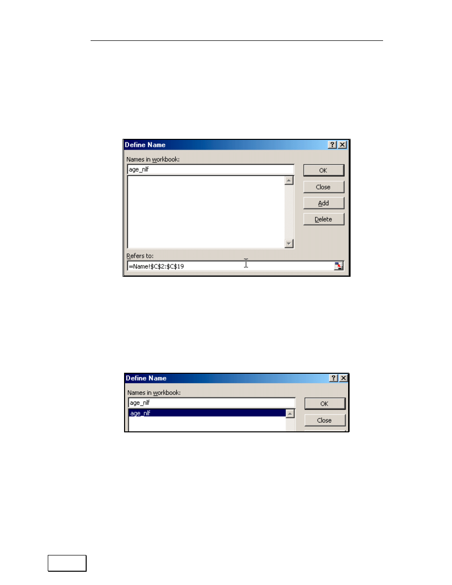
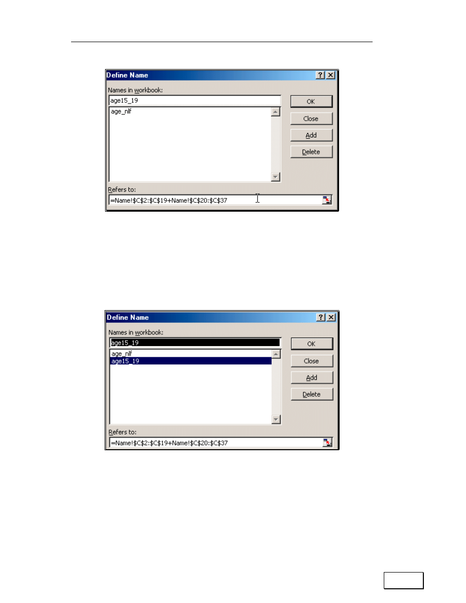
Pick the menu option “INSERT/NAME/DEFINE.” The dialog (user-input
form) that opens is shown in the next figure. Type the name of the range
into the text-box “Names in workbook” and the “Cell References” in the
box “Refers to:” See the next figure for an example.
Figure 27: The DEFINE NAMES dialog
Click on the button “Add.” The named range is defined. The name of a
defined range is displayed in the large text-box in the dialog. The next
figure illustrates this text.
Figure 28: Once added, the defined named range’s name can be seen in the large text-box
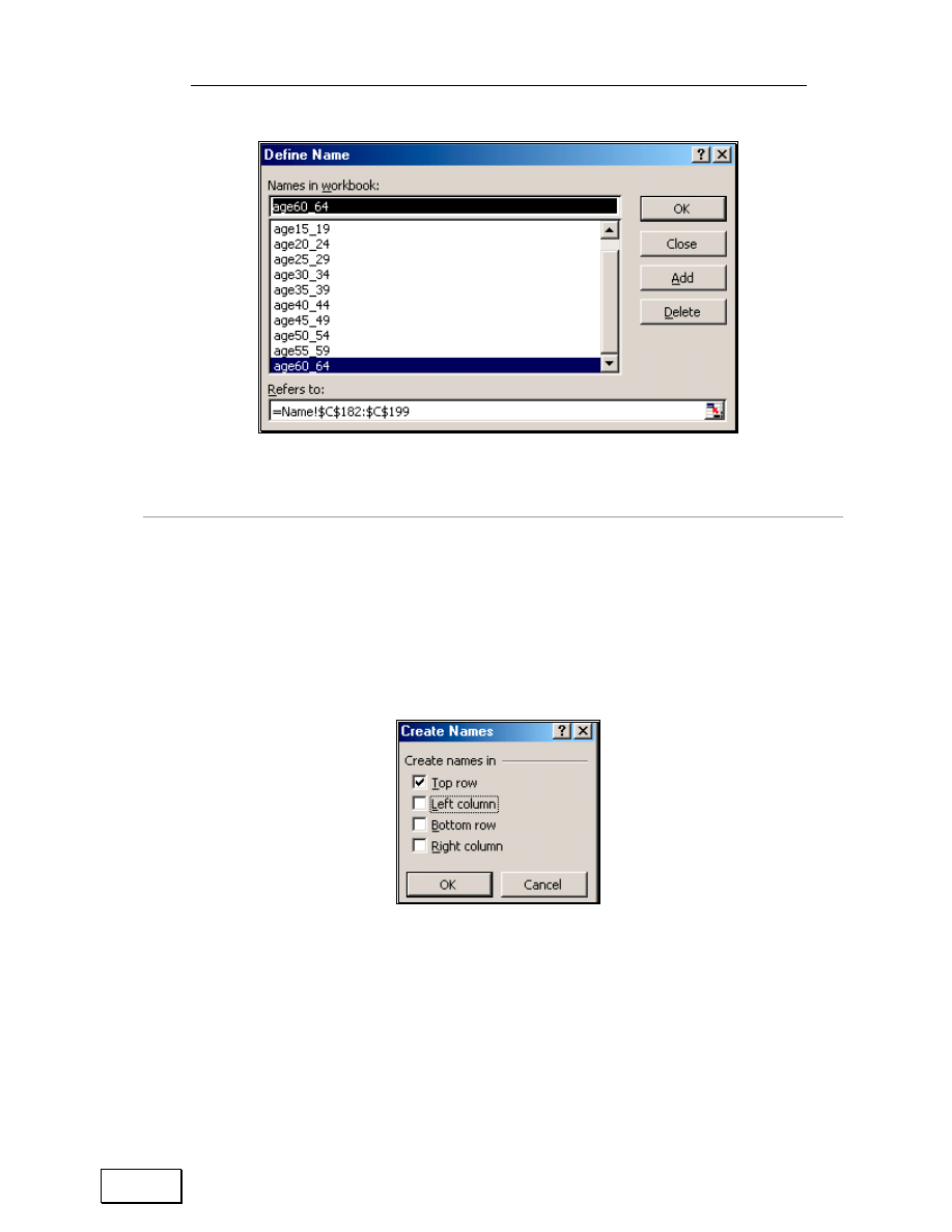
Several named ranges can be defined. A named range can represent
multiple blocks of cells.
Statistical Analysis with Excel
44
Figure 29: Defining a second named range. On clicking “Add,” the named range is defined, as
shown in the next figure.
You can view the ranges represent by any name. Just click on the name
in the central text-box and the range represented by the name will be
displayed in the bottom box.
Figure 30: Two named ranges are defined
Chapter 2: Copying/Cutting and pasting formulae
45
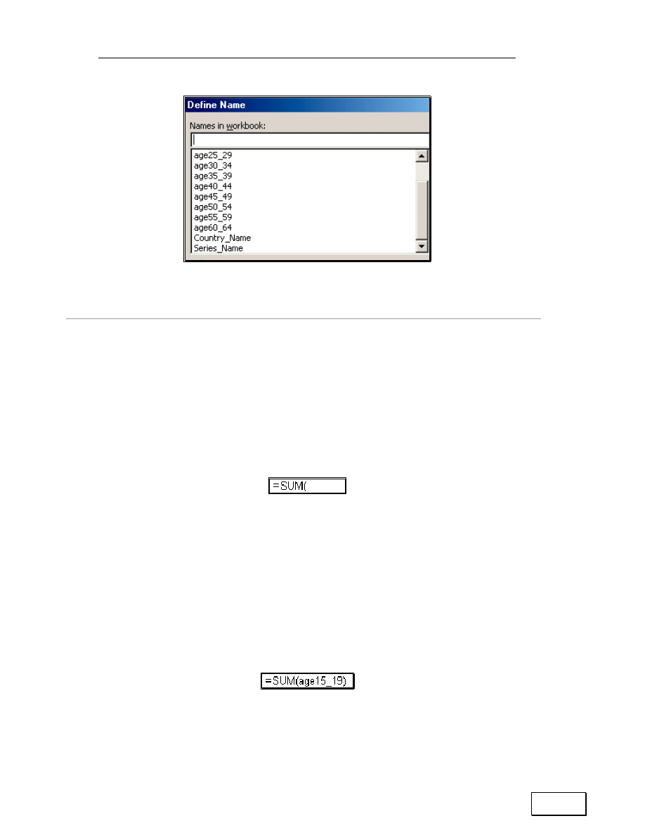
Figure 31: You can define many ranges. Just make sure that the names are explanatory and
not confusing.
Adding several named ranges in one step
If the first/last row/column in your ranges has the labels for the range,
then you can define names for all the ranges using the menu option
INSERT/NAMES/CREATE. The dialog is reproduced in the next figure.
Figure 32: CREATE NAMES
In our sample data set, I selected columns “A” and “B” and created the
names from the labels in the first row.
Statistical Analysis with Excel
46
Figure 33: The named ranges “Country_Name,” and “Series_Name” were defined in one step
using “Create Names”
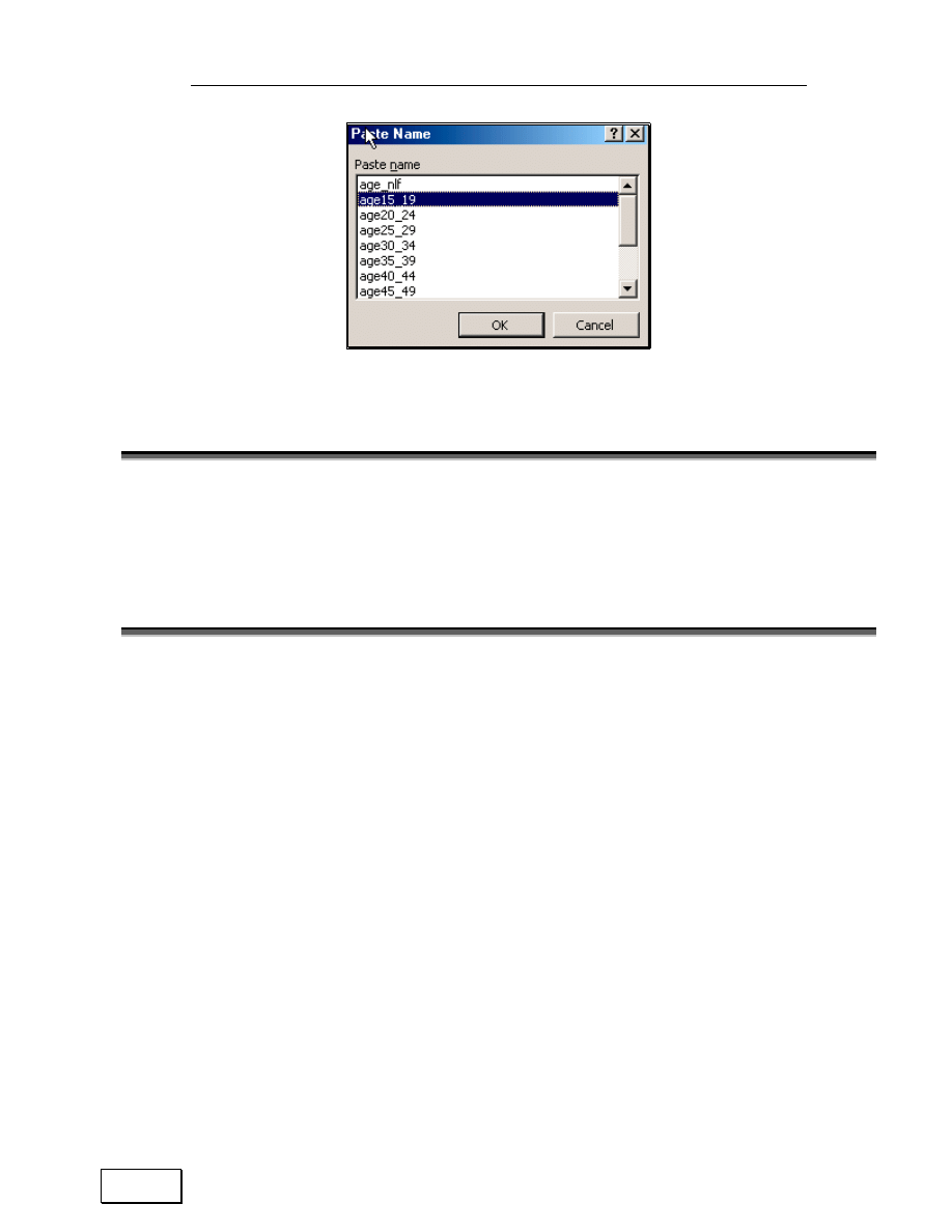
Using a named range
Named ranges are typically used to make formulas easier to read. The
named ranges could also be used in other procedures
Assume you want to sum several of the ranges defined above. One way to
sum them would be to select them one-by-one from the worksheet.
Another way is to use the menu option INSERT/NAME/PASTE to select
and paste the names of the ranges. The names are explanatory and
reduce the chances of errors in cell referencing.
A reference to the named range is pasted onto the formula as shown
below.
Chapter 2: Copying/Cutting and pasting formulae
47
Figure 34: Pasting named ranges
2.9
SELECTING ALL CELLS WITH FORMULAS THAT
EVALUATE TO A SIMILAR NUMBER TYPE
Volume 3: Excel– Beyond The Basics.
2.10
SPECIAL PASTE OPTIONS
2.10.A
PASTING ONLY THE FORMULA (BUT NOT THE FORMATTING
AND COMMENTS)
Refer to page 56 in chapter 3.
2.10.B
PASTING THE RESULT OF A FORMULA, BUT NOT THE
FORMULA ITSELF
Refer to page 53 in chapter 3.
Statistical Analysis with Excel
48
2.11
CUTTING AND PASTING FORMULAE
2.11.A
THE DIFFERENCE BETWEEN “COPYING AND PASTING”
FORMULAS AND “CUTTING AND PASTING” FORMULAS
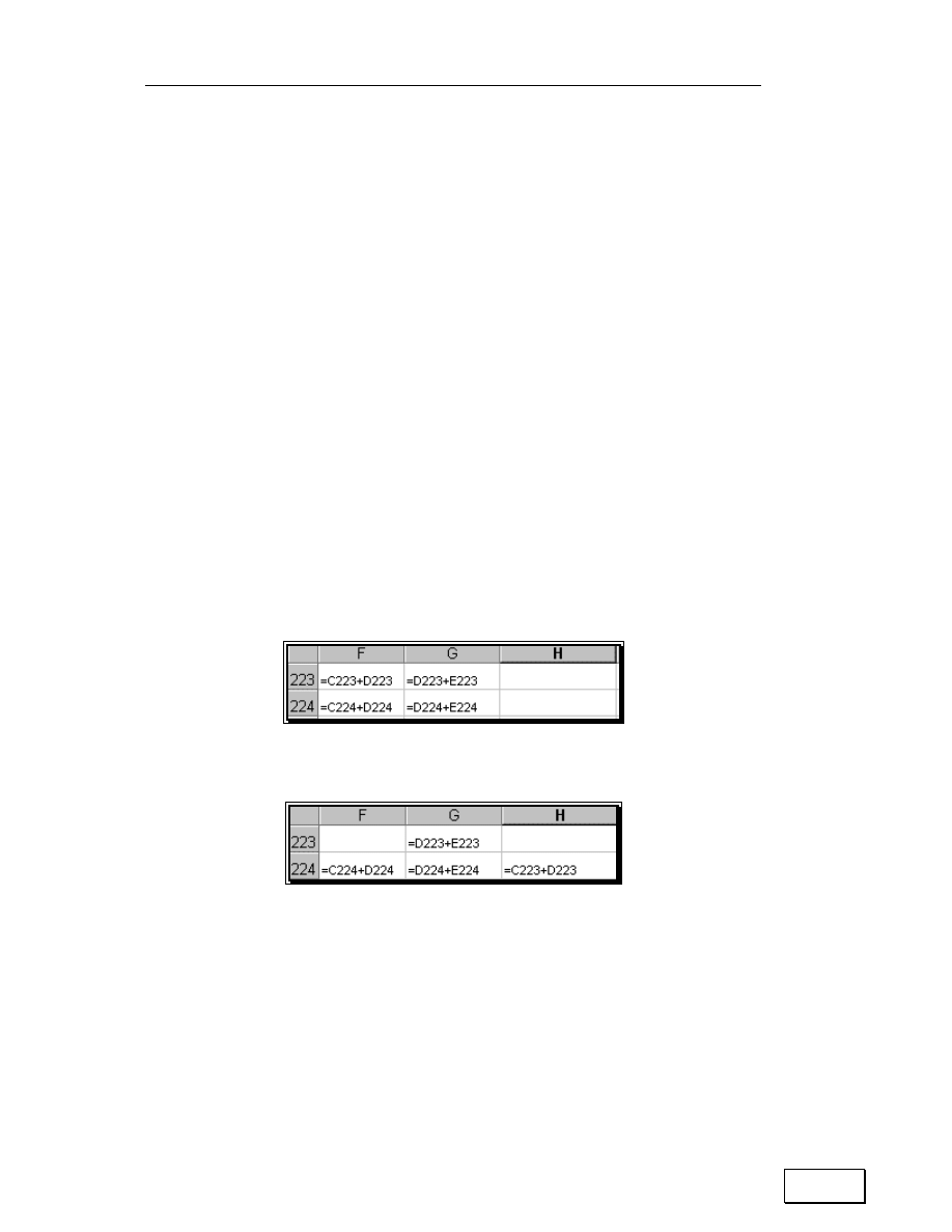
Click on cell F223, select the option EDIT/CUT, click on cell H224 and
choose the menu option EDIT/PASTE. The formula in the “pasted on” cell
is the same as was in the “cut from” cell. (The formula “=C223 + D223.”)
Therefore, there is no change in the cell references after cutting–and–
pasting. While copy–and–paste automatically adjusts for cell reference
differentials, cut–and–paste does not.
If you had used copy and paste, the formula in H224 would be “=D224 +
E224.”
Figure 35: Cut from cell F223
Figure 36: Paste into cell H223. Note that the cell references do not adjust.
After doing this, select the option EDIT/UNDO because I want to
maintain the formulas in F223— F235 (and not because it is required for
a cut and paste operation).

Chapter 2: Copying/Cutting and pasting formulae
49
2.12
CREATING A TABLE OF FORMULAS USING
DATA/TABLE
The menu option DATA/TABLE supposedly offers a tool for creating an X-
Y table of formula results. However, the method needs so much data
arrangement that it is no better than using a simple copy and paste
operation on cells!
2.13
SAVING TIME BY WRITING, COPYING AND PASTING
FORMULAS ON SEVERAL WORKSHEETS
SIMULTANEOUSLY
Refer to Volume 3: Excel– Beyond The Basics to learn how to work with
multiple worksheets. The section will request you to follow our example
of writing a formula for several worksheets together.

Page for Notes

Chapter 3: Paste Special
51
CHAPTER 3
PASTE SPECIAL
This chapter teaches the following topics:
— PASTING THE RESULT OF A FORMULA, BUT NOT THE
FORMULA
— OTHER SELECTIVE PASTING OPTIONS
— PASTING ONLY THE FORMULA (BUT NOT THE FORMATTING
AND COMMENTS)
— PASTING ONLY FORMATS
— PASTING DATA VALIDATION SCHEMES
— PASTING ALL BUT THE BORDERS
— PASTING COMMENTS ONLY
— PERFORMING AN ALGEBRAIC “OPERATION” WHEN PASTING
ONE COLUMN/ROW/RANGE ON TO ANOTHER
— MULTIPLYING/DIVIDING/SUBTRACTING/ADDING ALL CELLS
IN A RANGE BY A NUMBER
— MULTIPLYING/DIVIDING THE CELL VALUES IN CELLS IN
SEVERAL “PASTED ON” COLUMNS WITH THE VALUES OF
THE COPIED RANGE
— SWITCHING ROWS TO COLUMNS
This less known feature of Excel has some great options that save time
and reduce annoyances in copying and pasting.
Statistical Analysis with Excel
52
3.1
PASTING THE RESULT OF A FORMULA, BUT NOT
THE FORMULA
Sometimes one wants the ability to copy a formula (for example, “=C223 +
D223)”) but paste only the resulting value. (The example that follows will
make this clear.)
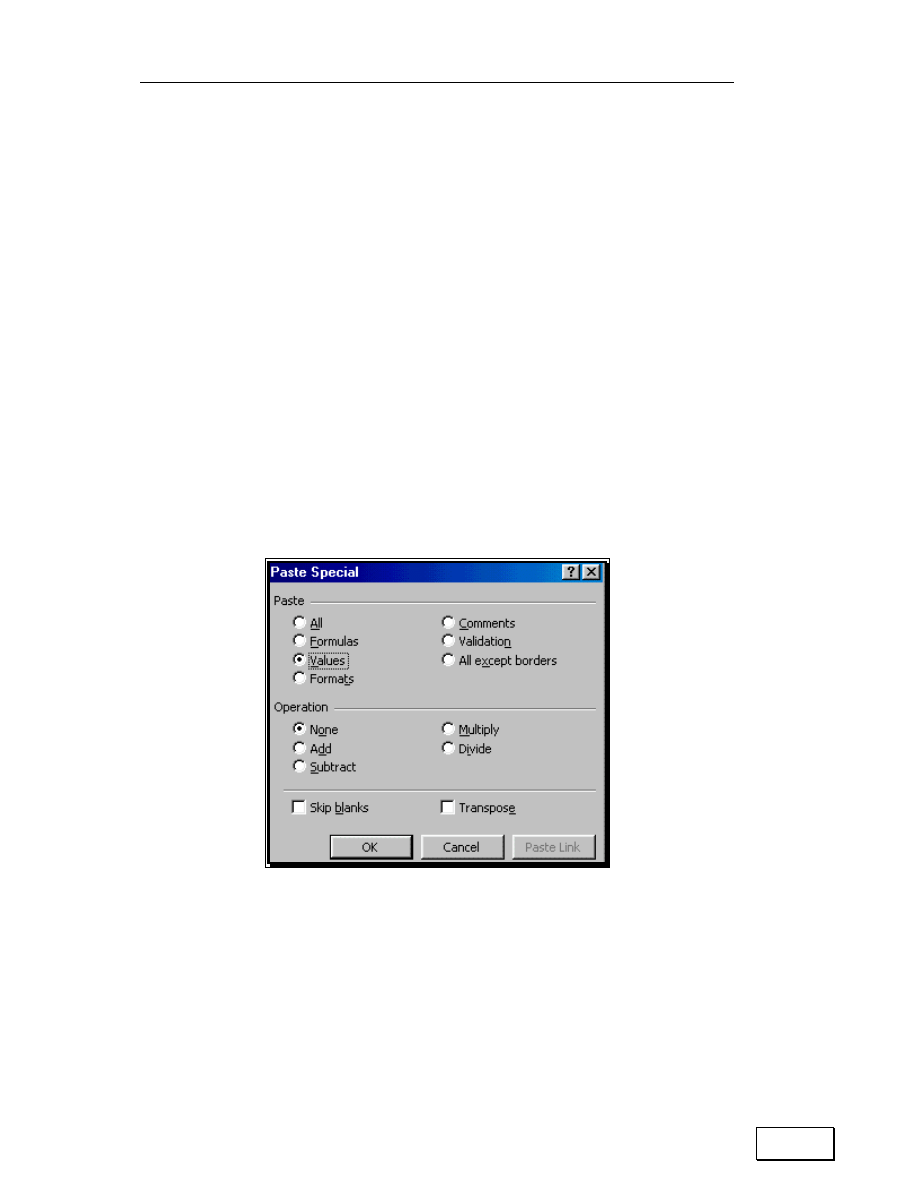
Select the range “F223:F235” on worksheet ““main.”
Choose the menu option FILE/NEW and open a new file. Go to any cell in
this new file and choose the menu option EDIT/PASTE SPECIAL.
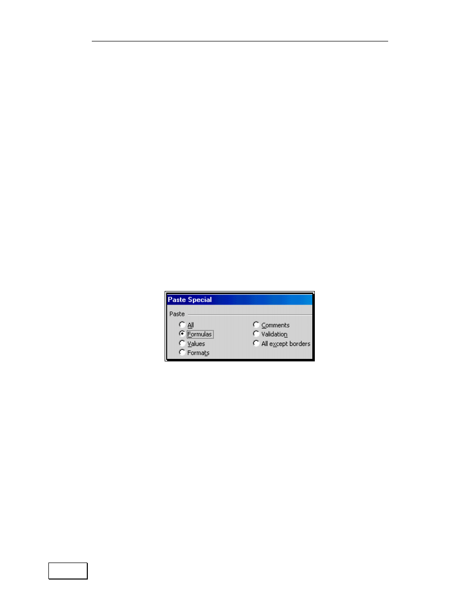
In the area “Paste,” choose the option “Values” as shown in Figure 37.
Figure 37: The PASTE SPECIAL dialog in Excel versions prior to Excel XP
Chapter 3: Paste Special
53
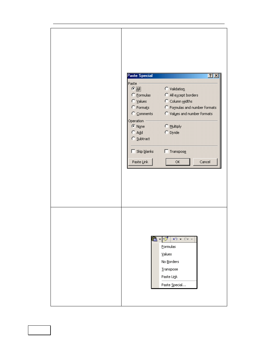
In Excel XP, the “Paste
Special” dialog has three
additional options:
•
Paste Formulas
and number
formats (and not
other cell
formatting like
font, background
color, borders, etc)
•
Paste Values and
number formats
(and not other cell
formatting like
font, background
color, borders, etc)
•
Paste only
“Column widths.”
Figure 38: “Paste Special” dialog In Excel XP,
In Excel XP, the “Paste” icon
provides quick access to some
types of “Paste Special.” The
options are shown in the next
figure.
The calculated values in the
“copied” cells are pasted. The
formula is not pasted. Try
the same experiment using
EDIT/PASTE instead of
EDIT/PASTE SPECIAL. The
usefulness of the former will
Figure 39: The pasting options can be accessed by
clicking on the arrow to the right of the “Paste” icon
Statistical Analysis with Excel
54
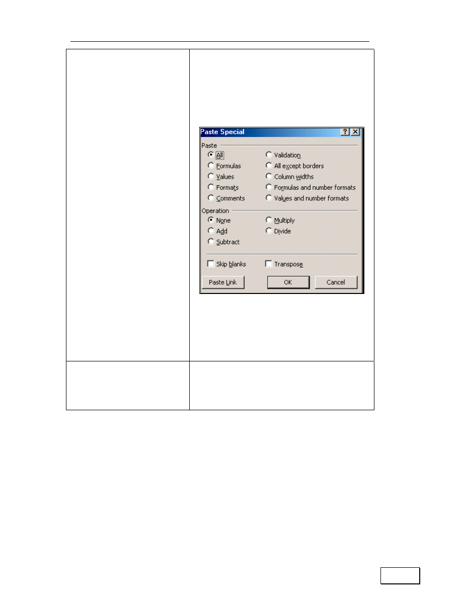
In Excel XP, the “Paste
Special” dialog has three
additional options:
•
Paste Formulas
and number
formats (and not
other cell
formatting like
font, background
color, borders, etc)
•
Paste Values and
number formats
(and not other cell
formatting like
font, background
color, borders, etc)
•
Paste only
“Column widths.”
Figure 38: “Paste Special” dialog In Excel XP,
be apparent.
Chapter 3: Paste Special
55
3.2
OTHER SELECTIVE PASTING OPTIONS
3.2.A
PASTING ONLY THE FORMULA (BUT NOT THE FORMATTING
AND COMMENTS)
Choose the option “Formulas” in the area “Paste” of the dialog (user-input
form) associated with the menu “EDIT/PASTE SPECIAL.” This feature
makes the pasted values free from all cell references. The “pasted on”
range will only contain pure numbers. The biggest advantage of this
option is that it enables the collating of formula results in different
ranges/sheets/workbooks onto one worksheet without the bother of
maintaining all the referenced cells in the same workbook/sheet as the
collated results.
Figure 40: Pasting formulas only
3.2.B
PASTING ONLY FORMATS
Choose the option “Formats” in the area “Paste” of the dialog associated
with the menu “EDIT/PASTE SPECIAL use the “Format Painter” icon. I
prefer using the icon.
Refer to Volume 1: Excel For Beginners for a discussion on the format
painter.

Statistical Analysis with Excel
56
3.2.C
PASTING DATA VALIDATION SCHEMES
Pick the option “Validation” in the area “Paste” of the dialog associated
with the menu “EDIT/PASTE SPECIAL.” Data validation schemes are
discussed in Volume 4: Managing & Tabulating Data in Excel. This
option can be very useful in standardizing data entry standards and rules
across an institution.
3.2.D
PASTING ALL BUT THE BORDERS
Choose the option “All except borders” in the area “Paste” of the dialog
associated with the menu “EDIT/PASTE SPECIAL.” All other formatting
features, formulae, and data are pasted. This option is rarely used.
3.2.E
PASTING COMMENTS ONLY
Pick the option “Comments” in the area “Paste” of the dialog associated
with the menu “EDIT/PASTE SPECIAL.” Only the comments are pasted.
The comments are pasted onto the equivalently located cell. For example,
a comment on the cell that is in the third row and second column that is
copied will be pasted onto the cell that is in the third row and second
column of the “pasted on” range. This option is rarely used.

Chapter 3: Paste Special
57
3.3
PERFORMING AN ALGEBRAIC “OPERATION” WHEN
PASTING ONE COLUMN/ROW/RANGE ON TO
ANOTHER
3.3.A
MULTIPLYING/DIVIDING/SUBTRACTING/ADDING ALL CELLS
IN A RANGE BY A NUMBER
Assume your data is expressed in millions. You need to change the units
to billions— that is, divide all values in the range by 1000. The complex
way to do this would be to create a new range with each cell in the new
range containing the formula “cell in old range/1000.” A much simpler
way is to use PASTE SPECIAL. On any cell in the worksheet, write the
number 1000. Click on that cell and copy the number. Choose the range
whose cells need a rescaling of units. Go to the menu option EDIT/PASTE
SPECIAL and choose “Divide” in the area Options. The range will be
replaced with a number obtained by dividing each cell by the copied cells
value!
The same method can be used to multiply, subtract or add a number to all
cells in a range
Figure 41: You can multiply (or add/subtract/divide) all cells in the “pasted on” range by
(to/by/from) the value of the copied cell

Statistical Analysis with Excel
58
3.3.B
MULTIPLYING/DIVIDING THE CELL VALUES IN CELLS IN
SEVERAL “PASTED ON” COLUMNS WITH THE VALUES OF THE
COPIED RANGE
You can use the same method to add/subtract/multiply/divide one
column’s (or row’s) values to the corresponding cells in one or several
“pasted on” columns (or rows).
Copy the cells in column E and paste special onto the
cells in columns C and D choosing the option “Add” in the area
“Operation” of the paste special dialog. (You can use EDIT/UNDO to
restore the file to its old state.)
3.4
SWITCHING ROWS TO COLUMNS
Choose any option in the “Paste” and “Operations” areas and choose the
option “Transpose.” If pasting a range with many columns and rows you
may prefer to paste onto one cell to avoid getting the error “Copy and
Paste areas are in different shapes.”

Page for Notes

Statistical Analysis with Excel
60
CHAPTER 4
INSERTING FUNCTIONS
This chapter teaches the following topics:
— A SIMPLE FUNCTION
— FUNCTIONS THAT NEED MULTIPLE RANGE REFERENCES
— WRITING A “FUNCTION WITHIN A FUNCTION“
— NEW IN EXCEL XP
— RECOMMENDED FUNCTIONS IN THE FUNCTION WIZARD
— EXPANDED AUTOSUM FUNCTIONALITY
— FORMULA EVALUATOR
— FORMULA ERROR CHECKING
4.1
BASICS
Excel has many in–built functions. The functions may be inserted into a
formula.
Accessing the functions dialog/wizard
(a) select the menu path INSERT/FUNCTION, or
(b) click on the function icon (see Figure 42)
Chapter 4: Inserting functions
61
Figure 42: The Function icon
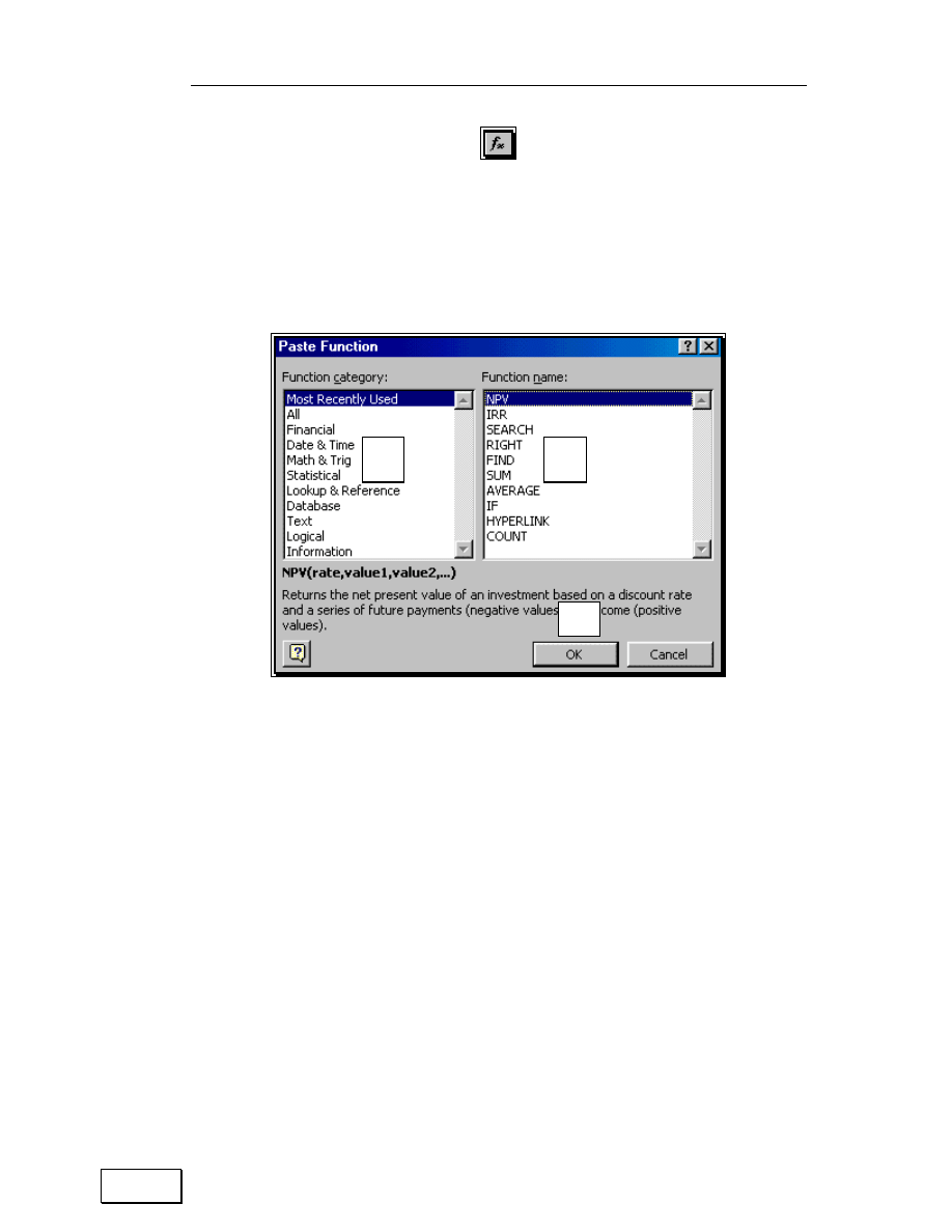
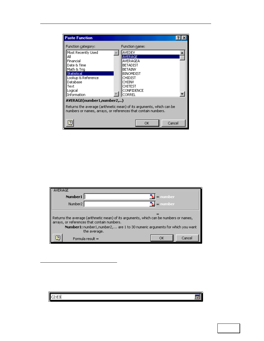
The “Paste Function” dialog (or wizard, because it is a series of dialogs)
opens. The dialog is shown in Figure 43.
Figure 43: Understanding the PASTE FUNCTION dialog
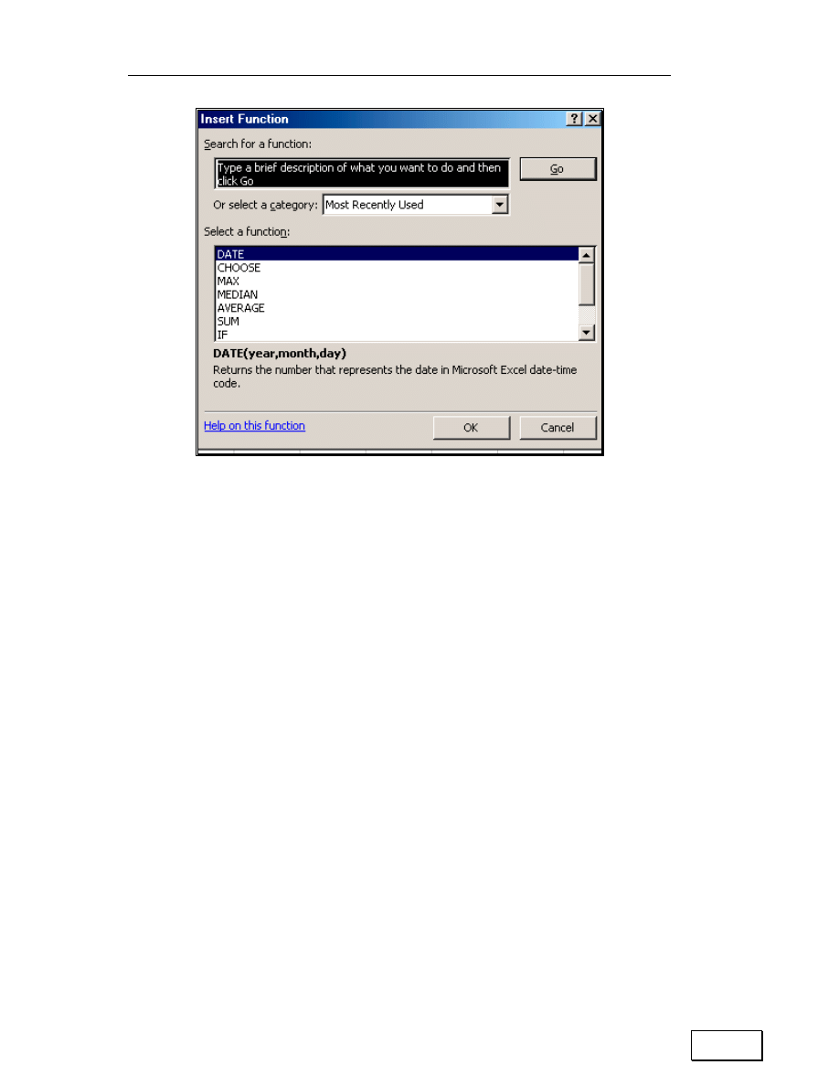
The equivalent dialog in the XP version of Excel is called INSERT
FUNCTION. (It is reproduced in the next figure below.) The dialog has
one new feature—a “Search for a function” utility. The “Function
category” is now available by clicking on the list box next to the label “Or
select a category.”
1
2
3
Statistical Analysis with Excel
62
Figure 44: The equivalent dialog in the XP version of Excel is called INSERT FUNCTION
This dialog has three parts:
(1) The area “Function category” on the left half shows the labels of
each group of functions. The group “Statistical” contains
statistical functions like “Average” and “Variance.” The group
“Math & Trig” contains algebra and trigonometry functions like
“Cosine.” When you click on a category name, all the functions
within the group are listed in the area “Function name.”
(2) The area “Function name” lists all the functions within the
category selected in the area “Function category.” When you
click on the name of a function, its formula, and description is
shown in the gray area at the bottom of the dialog.
(3) The area with a description of the function
Step 2 for using a function in a formula
Click on the “Function category” (in area 1 or the left half of the dialog)
Chapter 4: Inserting functions
63
that contains the function, then click on the function name in the area
“Function name” (in area 2 or the left half of the dialog) and then execute
the dialog by clicking on the button OK.
4.2
A SIMPLE FUNCTION
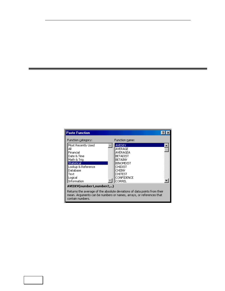
In my first example, I show how to select and use the function “Average”
which is under the category “Statistical.”
Choose the category “Statistical” as shown in Figure 45.
Figure 45: Choosing a function category
Choose the formula “Average” in the area “Function name.”
This is shown in Figure 46.
Execute the dialog by clicking on the button OK.
Statistical Analysis with Excel
64
Figure 46: Choosing a function name
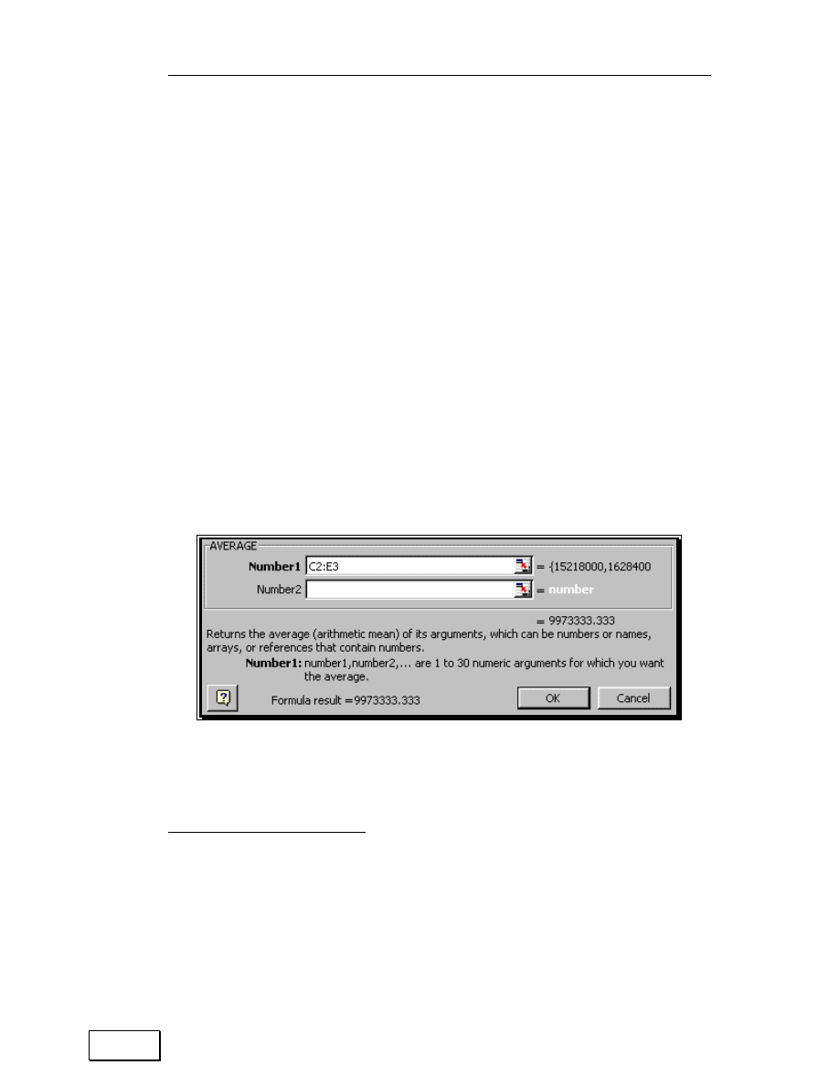
The dialog (user-input form) for the “Average” function opens.
For a pictorial reproduction of this, see Figure 47.
Figure 47: The dialog of the chosen function
Step 3 for inserting a function — defining the data
arguments/requirements for the function
Figure 48: Selecting the cell references whose values will be the inputs into the function
Chapter 4: Inserting functions
65
You have to tell Excel which cells contain the data to which you want to
apply the function “AVERAGE.” Click on the right edge of the text-box
“Number1”
6
. (That is, on the red–blue–and–white corner of the cell.) Go
to the worksheet that has the data you want to use and highlight the
range “C2 to E3.” Click on the edge of the text-box. (For a pictorial
reproduction of this, see Figure 48.)
You will be taken back to the “Average” dialog. Notice that — as shown in
Figure 49 — the cell reference “C2:E3” has been added.
Furthermore, note that the answer is provided at the bottom (see the line
“Formula result = 9973333.333”).
Execute the dialog by clicking on the button OK.
Figure 49: The completed function dialog
6
If you want to use non-adjacent ranges in the formula, then use the text-box “Number
2” for the second range. Excel will add more text-boxes once you fill all the available
ones. If the label for a text-box is not in bold then it is not essential to fill that text-
box. In the AVERAGE dialog shown in Figure 402, the label for the first text-box
(“Number 1”) is in bold—so it has to be filled. The label for the second text-box
(“Number 2”) is not in bold — so, it can be left empty.

Statistical Analysis with Excel
66
The formula is written into the cell and is shown in Figure 50.
Figure 50: The function is written into the cell
Press the ENTER key and the formula will be calculated.
You can work with this formula in a similar manner as a simple formula
— copying and pasting, cutting and pasting, writing on multiple
worksheets, etc.
If you remember the function name, you do not have to use
INSERT/FUNCTION. Instead, you can simple type in the formulas using
the keyboard. This method is faster but requires that you know the
function.
4.3
FUNCTIONS THAT NEED MULTIPLE RANGE
REFERENCES
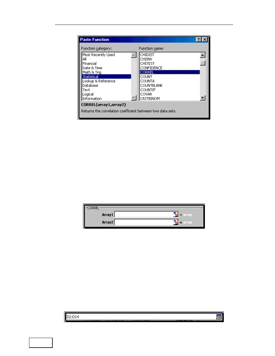
Some formulas need a multiple range reference. One example is the
correlation formula (“CORREL“). Assume, in cell J1, you want to
calculate the correlation between the data in the two ranges: “D2 to D14”
and “E2 to E14.”
Activate cell J1. Select the option INSERT/FUNCTION. Choose the
function category “Statistical.” In the list of functions that opens in the
right half of the dialog, choose the function “CORREL“ and execute the
dialog by clicking on the button OK.
Chapter 4: Inserting functions
67
Figure 51: Choosing the function CORREL
The CORREL dialog (shown in the next figure) opens. The function needs
two arrays (or series) of cells references. (Because the labels to both the
text-box labels are bold, both text-boxes have to be filled for the function
to be completely defined.) Therefore, the pointing to the cell references
has to be done twice as shown in Figure 53 and the next two figures.
Figure 52: The CORREL dialog
Choosing the first array/series
Click on the box edge of “Array1” (as shown in Figure 52.) Then go to the
relevant data range (D2 to D14 in this example) and select it.
Figure 53: Selecting the first data input for the function
Statistical Analysis with Excel
68
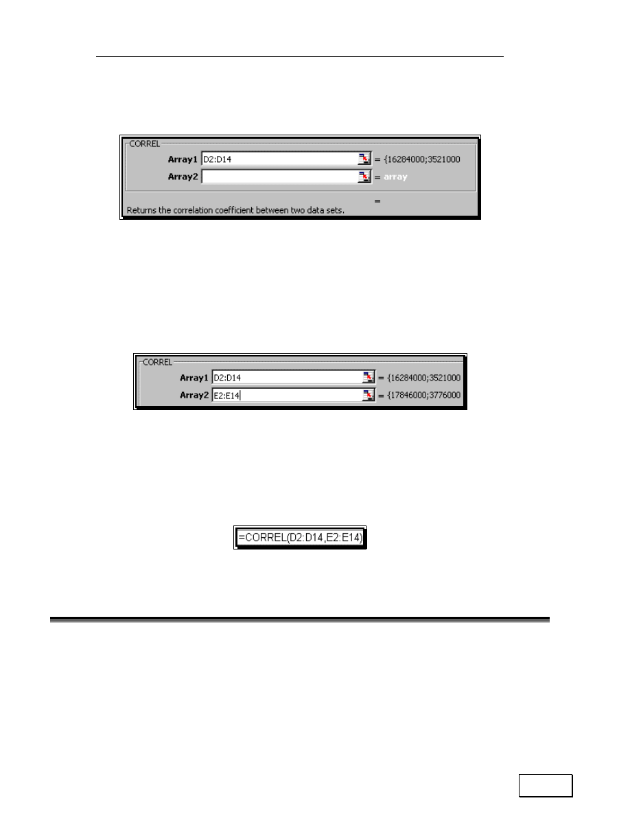
Repeat the same for “Array 2,” selecting the range “E2:E14” this time.
Figure 54: The first data input has been referenced
The formula is complete. The result is shown in the dialog in the area at
the bottom “Formula result.” Execute the dialog by clicking on the button
OK.
Figure 55: The second data input has also been referenced
Once the dialog closes, depress the ENTER key, and the function will be
written into the cell and its result evaluated/calculated.
Figure 56: The function as written into the cell.
4.4
WRITING A “FUNCTION WITHIN A FUNCTION”
I use the example of the CONFIDENCE function from the category
“Statistical.”
Choose the menu option INSERT/FUNCTION.

Chapter 4: Inserting functions
69
Choose the function category “Statistical.”
In the list of functions that opens in the right half of the dialog, choose the
function CONFIDENCE and execute the dialog by clicking on the button
OK.
Figure 57: Selecting the CONFIDENCE function
The Confidence dialog (user-input form) requires
7
three parameters: the
alpha, standard deviation, and sample size. First type in the alpha
desired as shown in Figure 58. (An alpha of “.05” corresponds to a 95%
confidence level while an alpha value of “:.1” corresponds to a confidence
interval of 90 %.)
Figure 58: Dialog for CONFIDENCE
7
We know that all three are necessary because their labels are in bold.
Statistical Analysis with Excel
70
Press the OK button.
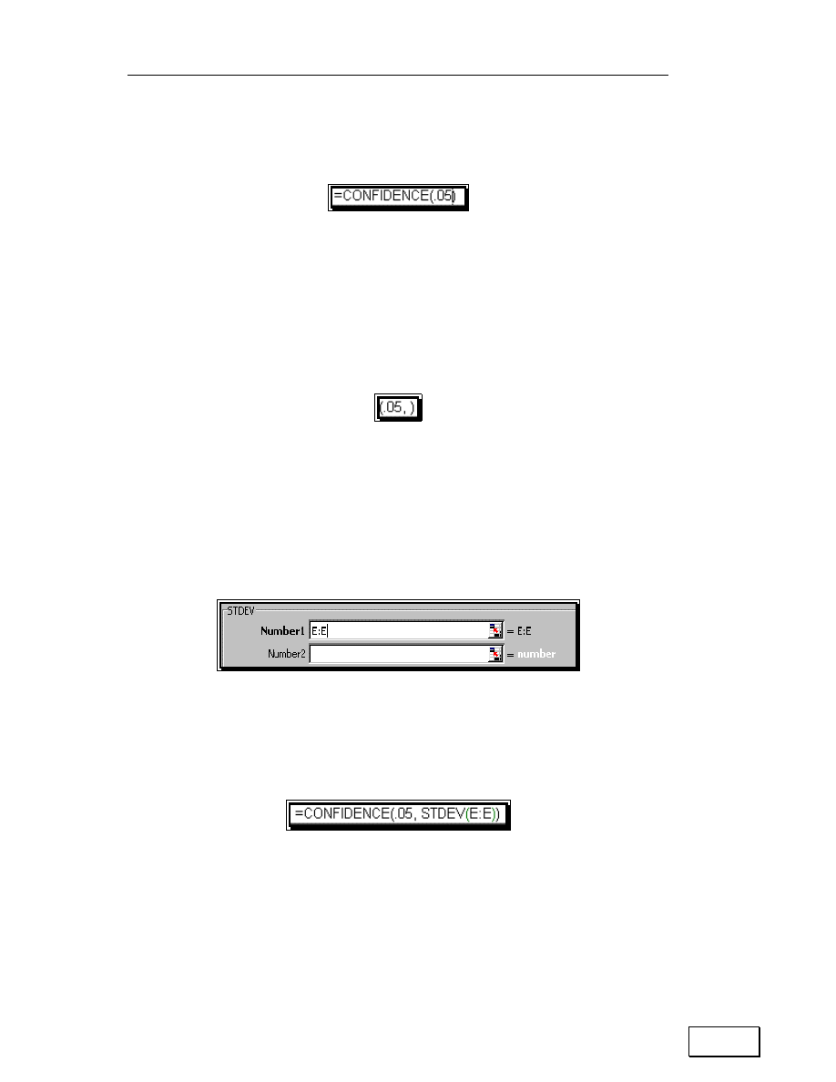
Figure 59: The first part of the function
Type a comma after the “.05” (see Figure 60) and then go to
INSERT/FUNCTION and choose the formula STDEV as shown in Figure
61.
Figure 60: Placing a comma before entering the second part
Choose the range for which you want to calculate the STDEV (for
example, the range “E:E”) and execute the dialog by clicking on the button
OK.
Figure 61: Using STDEV function for the second part of the function
The formula now becomes:
Figure 62: A function within a function
The main formula is still CONFIDENCE. The formula STDEV provides
one of the parameters for this main formula. The STDEV function is
nested within the CONFIDENCE function.
Chapter 4: Inserting functions
71
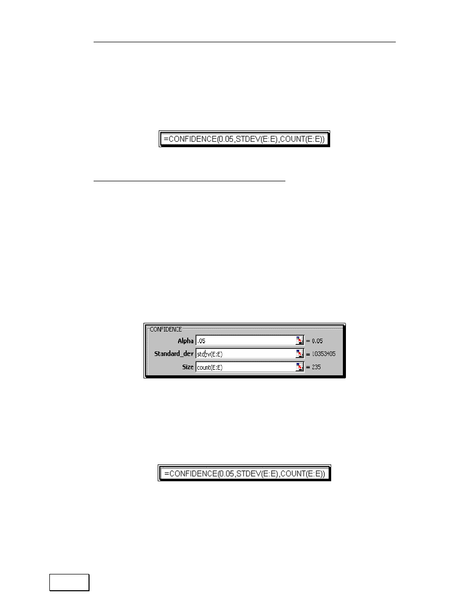
Type a comma, and then go to INSERT/FUNCTION and choose the
function “Count” from the function category “Statistical” to get the final
formula.
Figure 63: The completed formula
There are two other ways to write this formula.
Select the option INSERT/FUNCTION, choose the function
CONFIDENCE from the category “Statistical” and type in the formulae
“STDEV(E:E)” and “COUNT(E:E)” as shown in Figure 64.
This method is much faster but requires that you know the function
names STDEV and COUNT.
Figure 64: If sub-functions are required in the formula of a function, the sub-functions may be
typed into the relevant text-box of the function’s dialog
The third way to write the formula is to type it in. This is the fastest
method.
Figure 65: The result is the same
Statistical Analysis with Excel
72
4.5
NEW FUNCTION-RELATED FEATURES IN THE XP
VERSION OF EXCEL
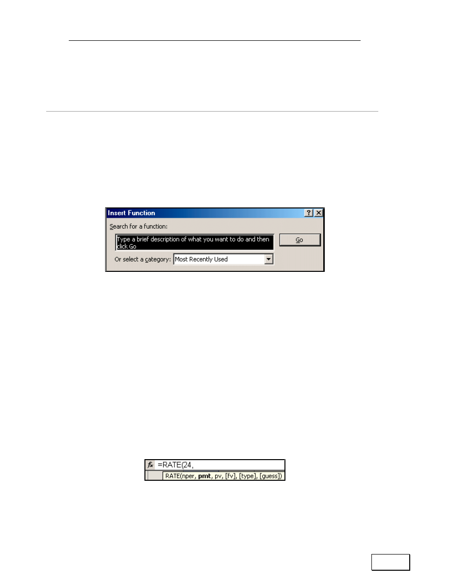
Searching for a function
Type a question (like “estimate maximum value”) into the box “Search for
a function” utility and click on the button “Go.” Excel will display a list of
functions related to your query.
Figure 66: Search for a function utility is available in the XP version of Excel
4.5.A
ENHANCED FORMULA BAR
After you enter a number or cell reference for the first function
“argument” (or first “requirement”) and type in a comma, Excel
automatically converts to bold format the next argument/requirement. In
the example shown in the next figure, Excel makes bold the font for the
argument placeholder pmt after you have entered a value for nper and a
comma.
Figure 67: The Formula Bar Assistant is visible below the Formula Bar
Similarly, the argument/requirement after pmt has a bold font after you
have entered a value or reference for the argument pmt
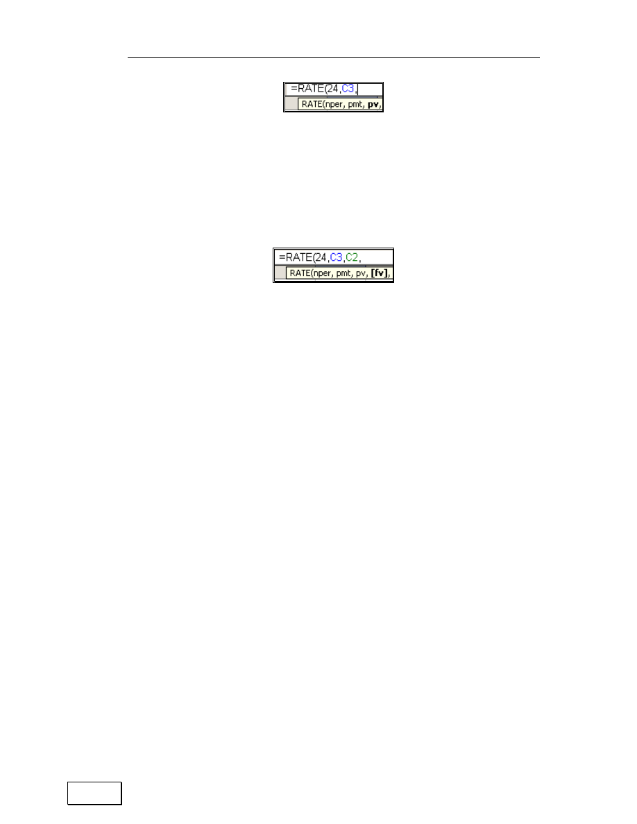
Chapter 4: Inserting functions
73
Figure 68: The next “expected” argument/requirement if highlighted using a bold font
The square brackets around the argument/requirement “fv” indicate that
the argument is optional. You need not enter a value or reference for the
argument.
Figure 69: An optional argument/requirement
4.5.B
ERROR CHECKING AND DEBUGGING
The basics of this topic are taught in the next chapter. Advanced features
are in Volume 3: Excel—Beyond the basics.

Page for Notes

Chapter 5: Tracing Cell References & Debugging Formula Errors
75
CHAPTER 5
TRACING CELL REFERENCES &
DEBUGGING FORMULA ERRORS
This short chapter demonstrates the following topics:
— TRACING THE CELL REFERENCES USED IN A FORMULA
— TRACING THE FORMULAS IN WHICH A PARTICULAR CELL
IS REFERENCED
— WATCH WINDOW
— ERROR CHECKING
— FORMULA EVALUATION
5.1
TRACING THE CELL REFERENCES USED IN A
FORMULA
Click on the cell that contains the formula whose references need to be
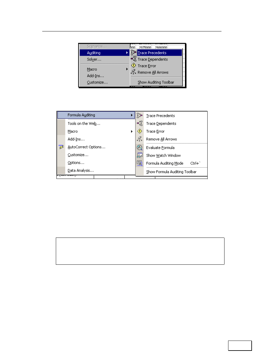
visually traced. Pick the menu option TOOLS/AUDITING/TRACE
PRECEDENTS. (For a pictorial reproduction of this, see Figure 70.)
Statistical Analysis with Excel
76
Figure 70: Tracing precedents. These options are from Excel versions prior to Excel XP.
Figure 71: Excel XP offers several error-checking and debugging tools.
As shown in Figure 72, blue arrows will trace the references.
If a group of cells is referenced, then the group will be marked by a blue
rectangle. The two rectangular areas are referenced in the formula.
In Volume 3: Excel- Beyond The Basics, you are taught the simple process
through which you can select all the cells whose formulas are precedents
of the active cell.
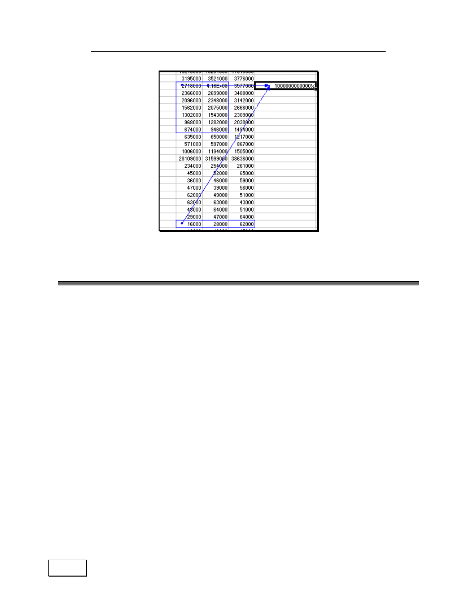
Chapter 5: Tracing Cell References & Debugging Formula Errors
77
Figure 72: The arrows define and trace all the cells/ranges referenced in the active cell
5.2
TRACING THE FORMULAS IN WHICH A
PARTICULAR CELL IS REFERENCED
You may want to do the opposite— see which formulas reference a
particular cell.
• First, click on the cell of interest.
•
Then, pick the menu option TOOLS/AUDITING/TRACE
DEPENDENTS as shown in Figure 73. Now the arrows will go
from the active cell to all the cells that have formulas that use
the active cell.
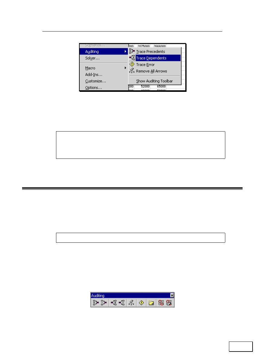
Statistical Analysis with Excel
78
Figure 73: Tracing Dependents. These options are from Excel versions prior to Excel XP.
Remove all the auditing arrows by following the menu path
TOOLS/AUDITING/REMOVE ALL ARROWS.
In Volume 3: Excel- Beyond The Basics you learn the simple process
through which you can select all the cells whose formulas are dependents
of the active cell.
5.3
THE AUDITING TOOLBAR
The
“
Auditing” toolbar opens automatically when you are using the
auditing option (TOOLS/AUDITING) to review formula references.
Refer to Volume 3: Excel- Beyond The Basics for details on using toolbars.
In the XP version of Excel, you can launch the toolbar through the menu
option TOOLS/AUDITING/SHOW FORMULA AUDITING TOOLBAR.
Figure 74: The “Auditing” toolbar
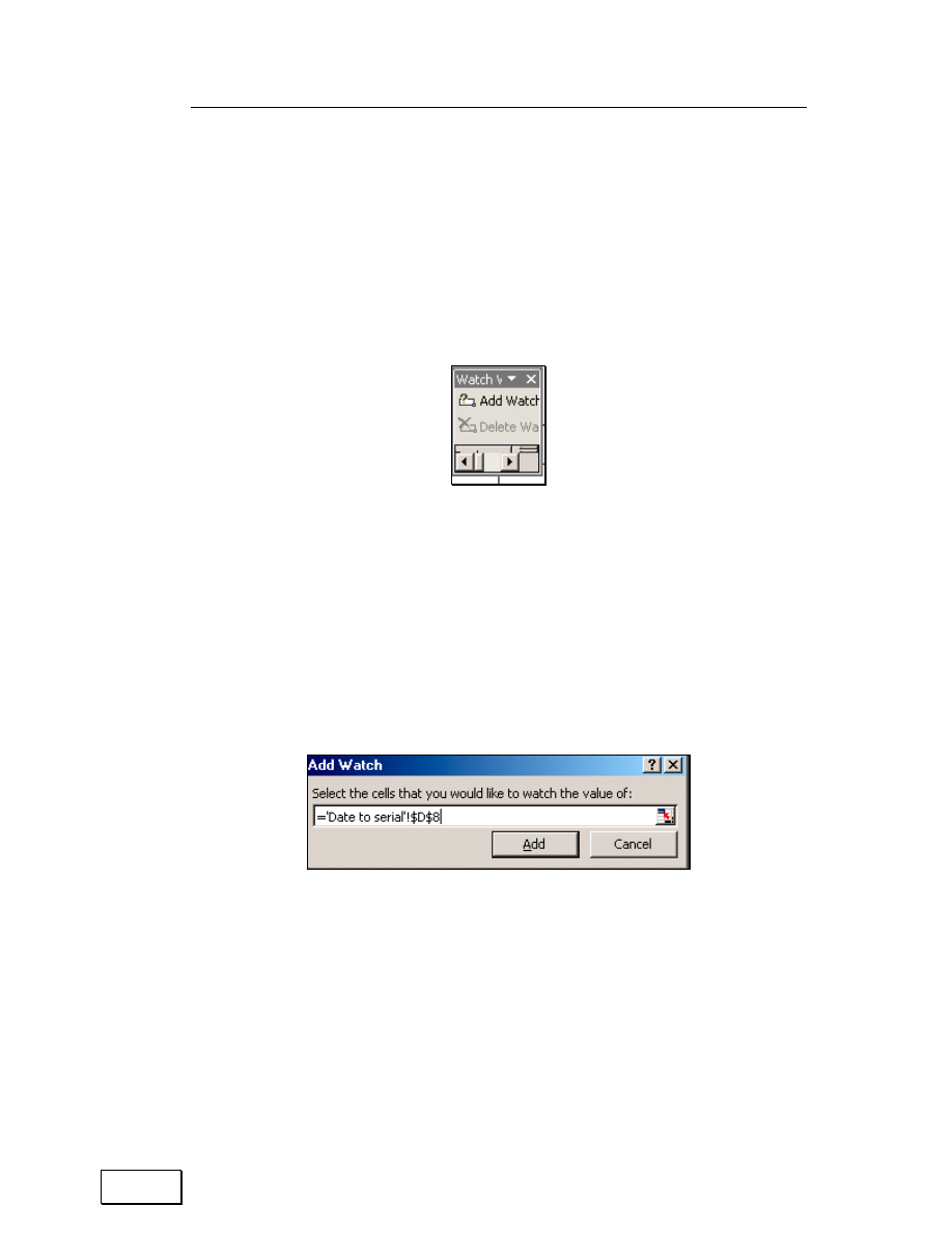
Chapter 5: Tracing Cell References & Debugging Formula Errors
79
5.4
WATCH WINDOW (ONLY AVAILABLE IN THE XP
VERSION OF EXCEL)
The window is accessed through the menu path TOOLS/ AUDITING/
SHOW WATCH WINDOW, or VIEW/ TOOLBARS/ WATCH WINDOW.
Figure 75: The Watch Window may not display correctly. Use the mouse to drag the walls of
the dialog to a workable size.
Add one cell on whose values you want to keep tabs.
The value will be shown in the Watch Window so that you can see the
value even if you are working on cells or sheets that are far from the cell
whose value is being
“
watched.”
Figure 76: Add Watch
You can add many cells to the Watch Window. Note that the Watch
Window provides precise information on the location of the cell being
watched and the formula in the cell. For example, the first watched cell is
on cell D8 in sheet
“
Date to serial” in the file
“
Date and Time.xls.” The
formula in the cell is
“
=DATE(F7, E7, D7)”.
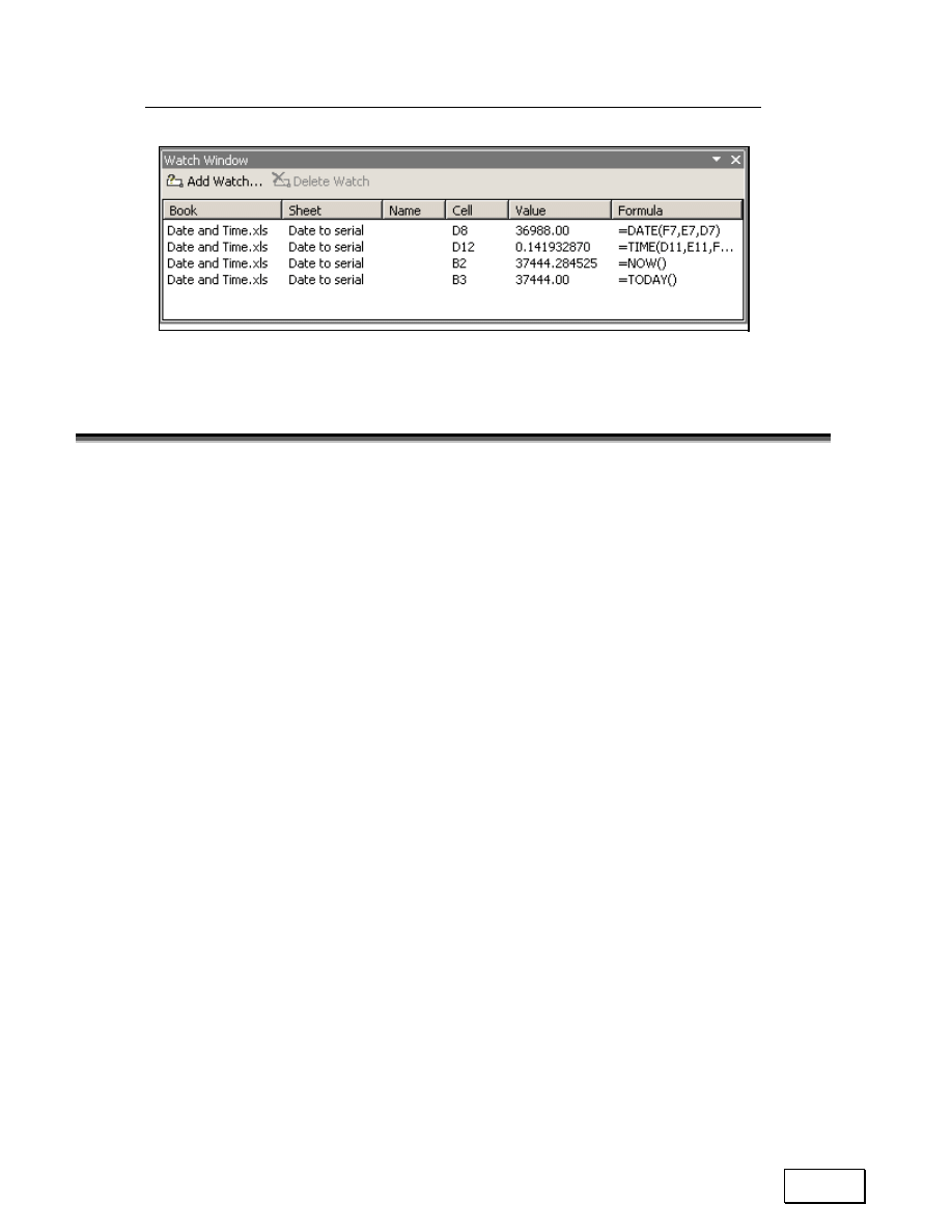
Statistical Analysis with Excel
80
Figure 77: You can add many cells to the Watch Window
5.5
ERROR CHECKING AND FORMULA EVALUATOR
(ONLY AVAILABLE IN THE XP VERSION OF EXCEL)
The tools are accessed through TOOLS/ERROR CHECKING and
TOOLS/FORMULA AUDITING/EVALUATE FORMULA.
The Error Checking dialog shows the formula in the cell as well as the
type of error. In this example, these are
“
=DEGREE(COS(C6))” and
“
Invalid Name Error,” respectively.
The button (
“
Help on this error”) links to a help file containing assistance
on understanding and debugging the error.
The button
“
Show Calculation Steps” links to a step-by-step debugger that
assists in catching the calculation step at which the error occurred.
This debugger has the same functionality as the Formula Auditor
(accessed through TOOLS/FORMULA AUDITING/EVALUATE
FORMULA).
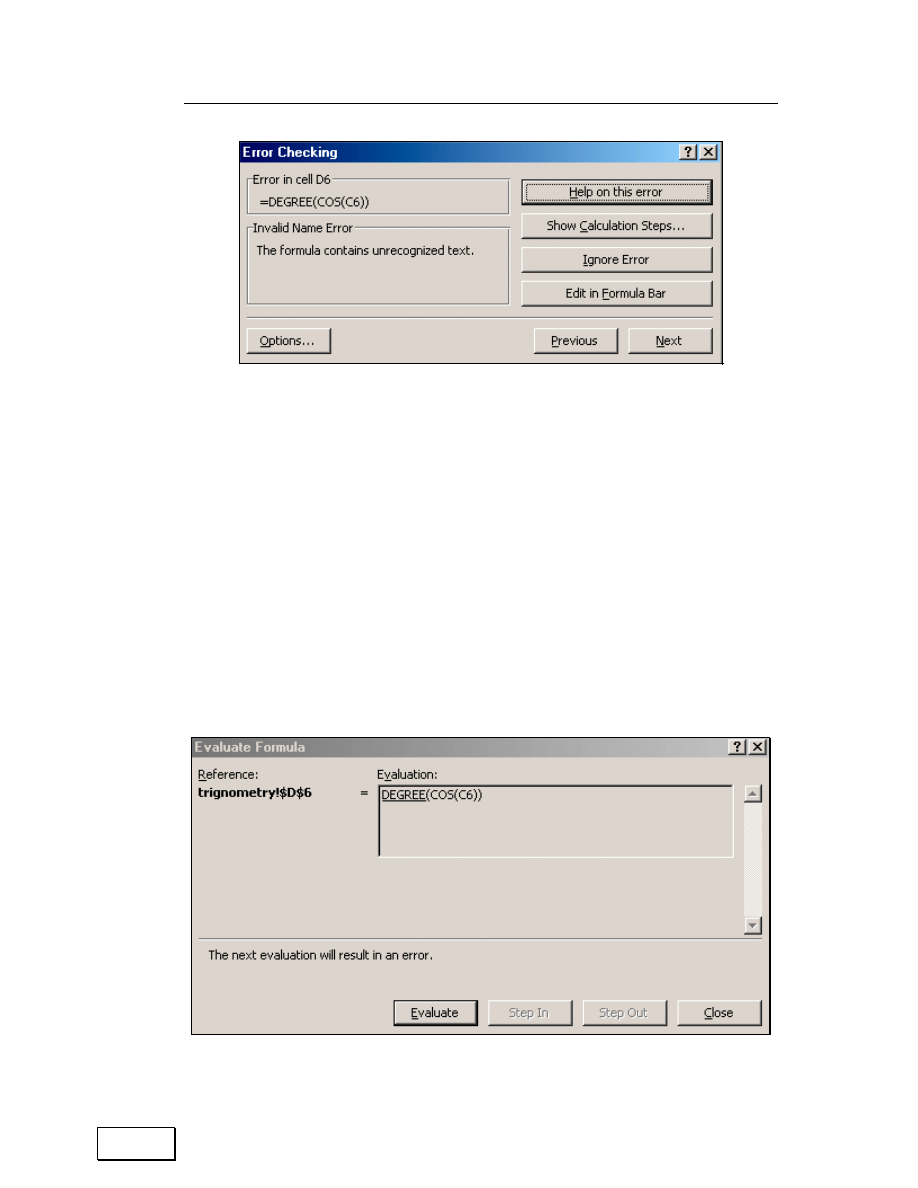
Chapter 5: Tracing Cell References & Debugging Formula Errors
81
Figure 78: The Error Checking dialog shows the formula in the cell as well as the type of error
The button
“
Ignore Error” keeps the error
“
as is.” The button Options
opens the dialog for setting error-checking options. The choices within the
dialog are listed in section 5.8.
The Formula Evaluator shows the step at which the first calculation error
occurred. This helps in identifying the primary problem. In this example,
no error has occurred in the formula part
“
COS(C6))”. The dialog informs
you that
“
The next evaluation (that is, calculation step), will result in an
error.”
Figure 79: The Formula Evaluator shows the step at which the first calculation error occurred
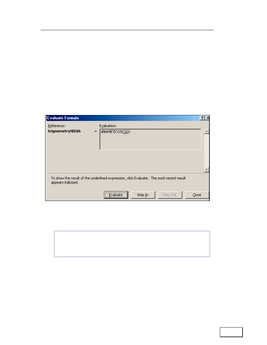
Statistical Analysis with Excel
82
After clicking on evaluate, you see that the error is in the formula part
“
DEGREE.” Excel also informs you of the type of error—
“
#NAME?”
suggests that
“
DEGREE” does not match the name of any Excel function.
(The correct function is
“
DEGREES.”)
The
“
COS
“
function is nested within the DEGREE function. Clicking on
“
Step In” will evaluate the nested function only.
Figure 80: After clicking on evaluate...
The
“
COS
“
function is evaluated. The function has no error.
If a function has more than two levels of nesting, then you can use the
“Step Out” button to evaluate the function at the higher level of
nesting.
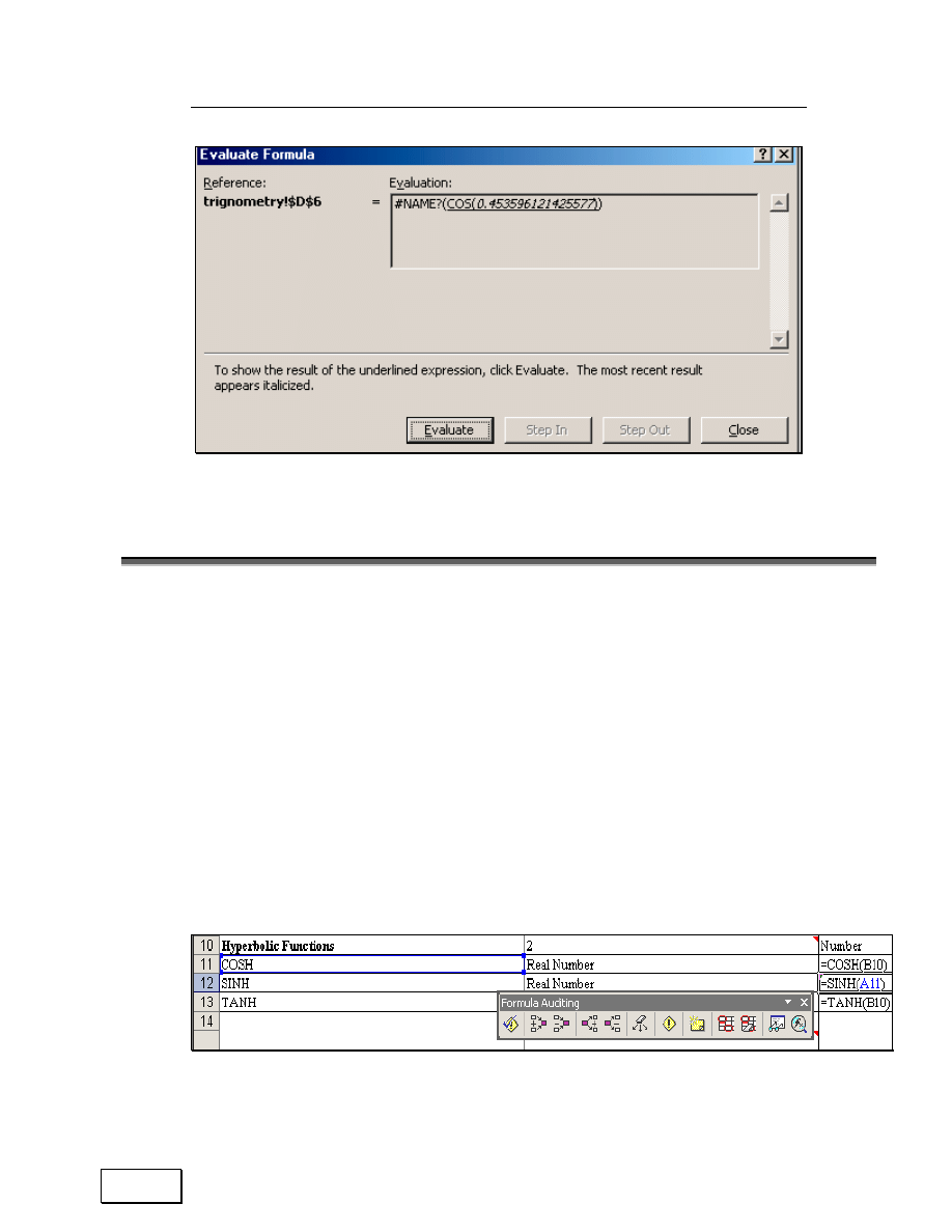
Chapter 5: Tracing Cell References & Debugging Formula Errors
83
Figure 81: The “COS“ function is evaluated
5.6
FORMULA AUDITING MODE (ONLY AVAILABLE IN
THE XP VERSION OF EXCEL)
This feature is accessed through TOOLS/FORMULA
AUDITING/FORMULA AUDITING MODE. After this mode is selected,
when you select a cell that has or is referenced by a formula, Excel
highlights the other referenced/referencing cells.
In addition, you have quick access (via the
“
Formula Auditing” toolbar) to
all the Auditing tools discussed earlier in this chapter.
Figure 82: Formula Auditing Mode
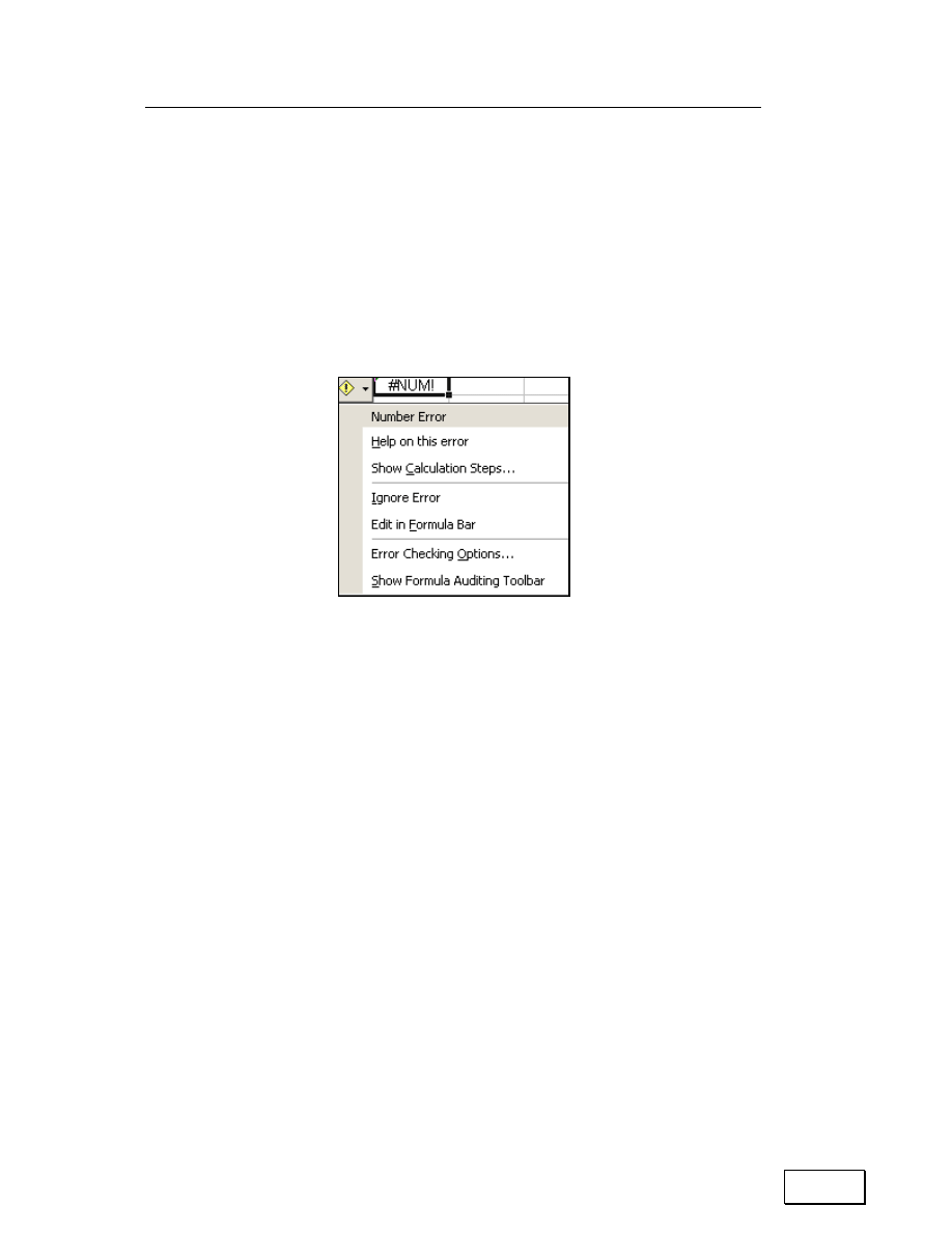
Statistical Analysis with Excel
84
5.7
CELL-SPECIFIC ERROR CHECKING AND
DEBUGGING
On every cell whose value evaluates to an error value, you will see a small
icon with a
“
!” image and a downward arrow. Click on the arrow to obtain
assistance for debugging the error.
Figure 83: Cell-specific Error Checking and Debugging
In the example shown in the figure, the options show:
— the error type (
“
Number Error”),
— a link to assistance on understanding and debugging the error (
“
Help
on this error”),
— a step-by-step debugger to catch the calculation step at which the error
occurred (
“
Show Calculation Steps”),
— the option to ignore and thereby keep the error as is (
“
Ignore Error”),
— a link to directly edit the formula in the cell (
“
Edit in Formula Bar”),
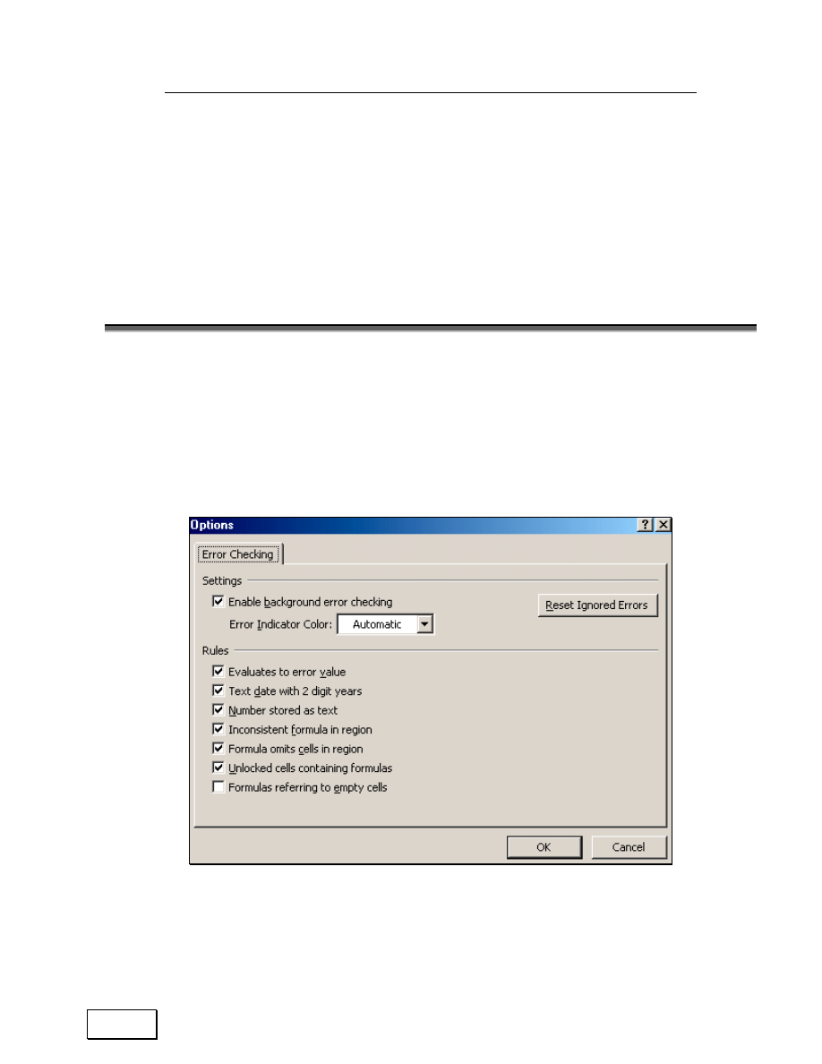
Chapter 5: Tracing Cell References & Debugging Formula Errors
85
— the overall error-checking options (
“
Error Checking Options”), and
— direct access to the Formula Auditing Toolbar (
“
Show Formula
Auditing Toolbar”) and, thereby, to all the features of Auditing (these
features are taught in this chapter)
5.8
ERROR CHECKING OPTIONS
The Error Checking options can be assessed through
TOOLS/OPTIONS/ERROR CHECKING or through TOOLS/ERROR
CHECKING/OPTIONS. The dialog is reproduced in the next figure.
Figure 84: Error Checking options
You can inform Excel to show as an error any cell: that contains:

Statistical Analysis with Excel
86
• A formula that evaluates to an error value
• A formula that refers to an empty cell
• A formula that is not consistent with the other formulas and cell
references in neighboring cells
• A two-digit year (like
“
02”) instead of a four-digit year (like
“
2002”)
•
A number stored as text
The other options are beyond the scope of this book. I recommend sticking
with the default settings reproduced in the next figure.

Page for Notes

Statistical Analysis with Excel
88
CHAPTER 6
FUNCTIONS FOR BASIC STATISTICS
This chapter discusses the following topics:
— “AVERAGED” MEASURES OF CENTRAL TENDENCY
— AVERAGE, TRIMMED MEAN, HARMONIC MEAN, GEOMETRIC
MEAN
— LOCATION MEASURES OF CENTRAL TENDENCY
— MEDIAN, MODE
— OTHER LOCATION PARAMETERS
— QUARTILE, PERCENTILE
— MAXIMUM VALUE, MINIMUM VALUE, LARGE, SMALL
— RANK OR RELATIVE STANDING OF EACH CELL WITHIN THE
RANGE OF A SERIES
— MEASURES OF DISPERSION (STANDARD DEVIATION &
VARIANCE)
— STDEV, VAR, STDEVA, VARA, STDEVP, VARP, STDEVPA,
VARPA
— SHAPE ATTRIBUTES OF THE DENSITY FUNCTION
— SKEWNESS, KURTOSIS
— FUNCTIONS ENDING WITH AN “A” SUFFIX
I am presuming that the reader is familiar with basic statistical functions
and/or has access to a basic statistics reference for learning more about

Chapter 6: Functions for Basic Statistics
89
each function.
6.1
“AVERAGED” MEASURES OF CENTRAL TENDENCY
These set of functions perform some type of averaging to measure a
“
mean” value. You may want to use the Trimmed Mean function to
estimate an average that excludes the extreme values of the data series.
The Harmonic Mean estimates the averages of the reciprocals of the
numbers in the series. The Geometric Mean is used to average rates of
change.
Samples will be available at
http://www.vjbooks.net/excel/samples.htm
.
6.1.A
AVERAGE
The function calculates the simple arithmetic average of all cells in the
chosen range.
Menu path to function: Go to the menu option INSERT/FUNCTION and
choose the formula
“
AVERAGE the function category STATISTICAL.
Figure 85: AVERAGE function

Statistical Analysis with Excel
90
Data requirements: The X values can be input as references to one or more
ranges that may be non–adjacent. The second range can be referenced in
the first text-box
“
Number1” after placing a comma after the first range,
or it could be referenced in the second text-box
“
Number2.” If you use the
second text-box, then a third text-box
“
Number3” will automatically open.
(As you fill the last visible box, another box opens until the maximum
number of boxes — 30 — is reached.)
The function does not count invalid cell values when counting the number
of X values. The X values can take any real number value.
6.1.B
TRIMMEAN (“TRIMMED MEAN”)
This function is a variation of the average or mean. This function
calculates the average for a set of X values after removing
“
extreme
values” from the set. The excluded cells are chosen by the user based on
the extremity (from mean/median) of the values in the range.
TRIMMEAN calculates the mean taken by excluding a percentage of data
points from the top and bottom tails of a data set. The user decides on the
percentage of extreme values to drop. For symmetry, TRIMMEAN
excludes a set of values from the top and bottom of the data set before
moving on to the next exclusion.
Menu path to function: INSERT/FUNCTION/STATISTICAL/TRIMMEAN.
Data requirements: The X values can be input as references to one or more
ranges that may be non–adjacent. The function does not count invalid cell
values when counting the number of X values. The X values can take any
real number value.
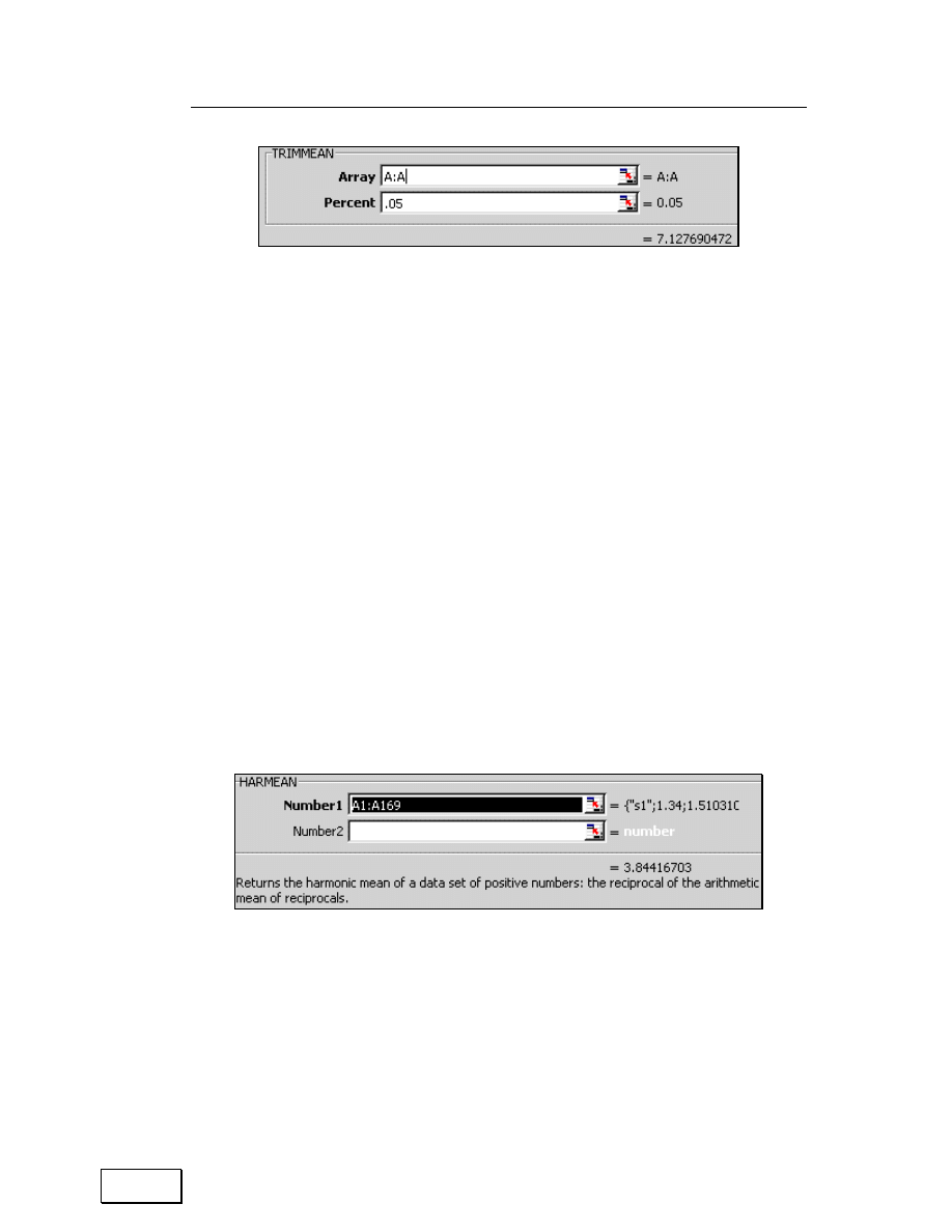
Chapter 6: Functions for Basic Statistics
91
Figure 86: TRIMMEAN (Trimmed Mean)
In the dialog (shown above), Percent is the fractional number of data
points to exclude from the calculation. Percent must be greater than zero
and less than one.
6.1.C
HARMEAN (“HARMONIC MEAN”)
The function calculates the harmonic mean of all cells in the chosen
range(s). The harmonic mean is the reciprocal of the arithmetic mean of
reciprocals. In the formula below, H is the harmonic mean, n the
sample/range size and the Y’s are individual data values.
Menu path to function: INSERT/FUNCTION/STATISTICAL/HARMEAN.
Figure 87: HARMEAN (Harmonic Mean)
Data requirements: The X values can take any real number value except
zero.
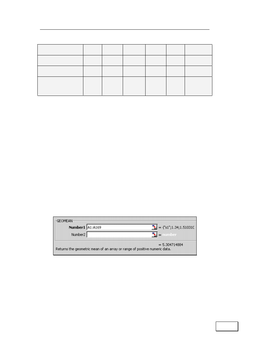
Statistical Analysis with Excel
92
Table 10: Comparing the results of the functions Average, Trimmed Mean
and Harmonic Mean
Function
s1
s2
x1
x2
x3
x4
Average/mean
7.32
7.23
1173.00
14.55
0.17
1158.45
Trimmed Mean
7.13
7.00
1173.00
14.42
0.02
1158.71
Harmonic Mean
3.84
3.18
120.17
13.52
0.01
#NUM!
Harmonic mean for x4 is zero because one value of x4 is not positive.
6.1.D
GEOMEAN (“GEOMETRIC MEAN”)
This function is typically used to calculate average growth rate given
compound interest with series rates. In general, the function is good for
estimating average growth or interest rates.
Menu path to function: INSERT/ FUNCTION/ STATISTICAL/
GEOMEAN. Data requirements: All values should be positive.
Figure 88: GEOMEAN (Geometric Mean)
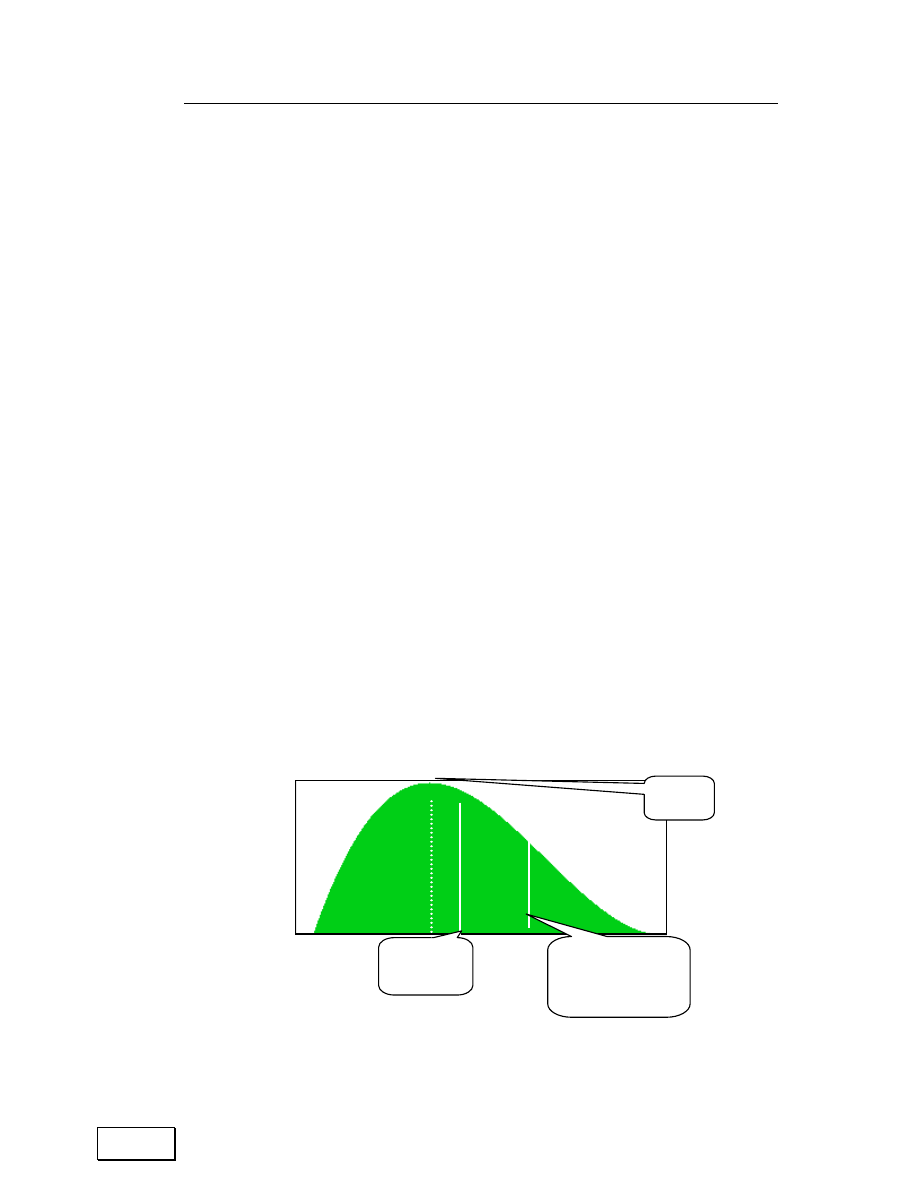
Chapter 6: Functions for Basic Statistics
93
6.2
LOCATION MEASURES OF CENTRAL TENDENCY
(MODE, MEDIAN)
The Median and — less often — the Mode are also used for estimating the
central tendency of a series. The Median is much better in situations
where, either:
(a) A few extreme highs or lows are influencing the Mean (note that
the TRIMMEAN or Trimmed Mean function shown in the
previous section can reduce the chance of extreme values over-
influencing a Mean estimate), or
(b) The central tendency is required to obtain the mid-point of
observed values of the data series as in the
“
Median Voter”
models, which are used to know if the
“
Median Voter” threshold is
crossed in support of a point on the nominee’s agenda. (In a two-
person face-off, any more than the Median vote will result in a
greater than 50% majority).
Samples will be available at
http://www.vjbooks.net/excel/samples.htm
.
Figure 89: Some location indicators
75
th
percentile
(or 3
rd
quartile)
Median4
Mode

Statistical Analysis with Excel
94
6.2.A
MEDIAN
The Median is the number in the middle of a set of numbers. It is the 50
th
percentile.
Menu path to function: INSERT/FUNCTION/STATISTICAL/MEDIAN.
Data requirements: Any array/range with real numbers.
6.2.B
MODE
This function returns the most frequently occurring value in a range.
Menu path to function: INSERT/FUNCTION/STATISTICAL/MODE.
Data requirements: Any array/range with real numbers. The range has to
contain duplicate data values.
6.3
OTHER LOCATION PARAMETERS (MAXIMUM,
PERCENTILES, QUARTILES, OTHER)
Other useful location indicators for key points in a series are the
quartiles, percentiles, maximum value, minimum value, the Kth largest
value, and the rank.
Samples will be available at
http://www.vjbooks.net/excel/samples.htm
.

Chapter 6: Functions for Basic Statistics
95
6.3.A
QUARTILE
This function calculates a quartile of a data series.
QUARTILE (Data, Quartile)
Choose the quartile you desire to obtain. The five quartiles are shown in
the next table.
Table 11: Choosing the Quartile
Quartile value of…
Calculates the...
0
0.0….1% ile
1
First quartile (25th percentile)
2
Median value (50th percentile)
3
Third quartile (75th percentile)
4
Fourth quartile (99.9x%ile)
Menu path to function: INSERT/FUNCTION/STATISTICAL/QUARTILE.
Data requirements: Any array/range with real numbers. Note: the data
series has to contain between 1 and 8,191 data points
6.3.B
PERCENTILE
This function returns the P
th
percentile of values in a data series. You can
use this function to establish a threshold of acceptance. For example, you
can prefer to examine candidates who score above the 95th percentile will
qualify for a scholarship.
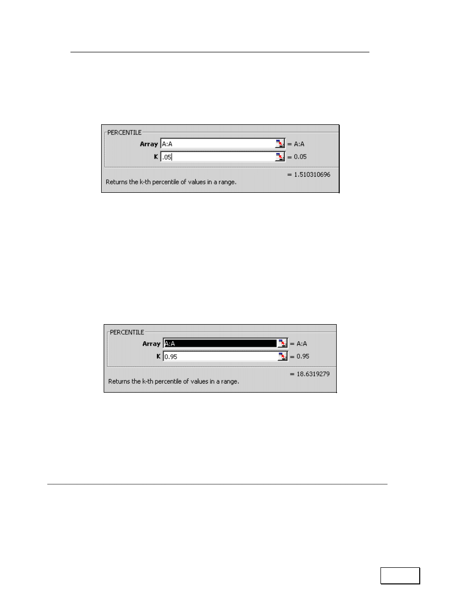
Statistical Analysis with Excel
96
Menu path to function:
INSERT/FUNCTION/STATISTICAL/PERCENTILE.
Figure 90: Estimating the 5th percentile. K is the percentile value in the range 0 to 1.
Data requirements: Any array/range with real numbers. If the data array
is empty or contains more than 8,191 data points, PERCENTILE returns
the” #NUM!” error value. If K is not a multiple of (1/(n — 1)), then Excel
interpolates the value at the Kth percentile.
Figure 91: Estimating the 95th percentile
6.3.C
MAXIMUM, MINIMUM AND “KTH LARGEST”
MAX (“Maximum value”)
MAX and MAXA: The functions calculate the largest value in a series.
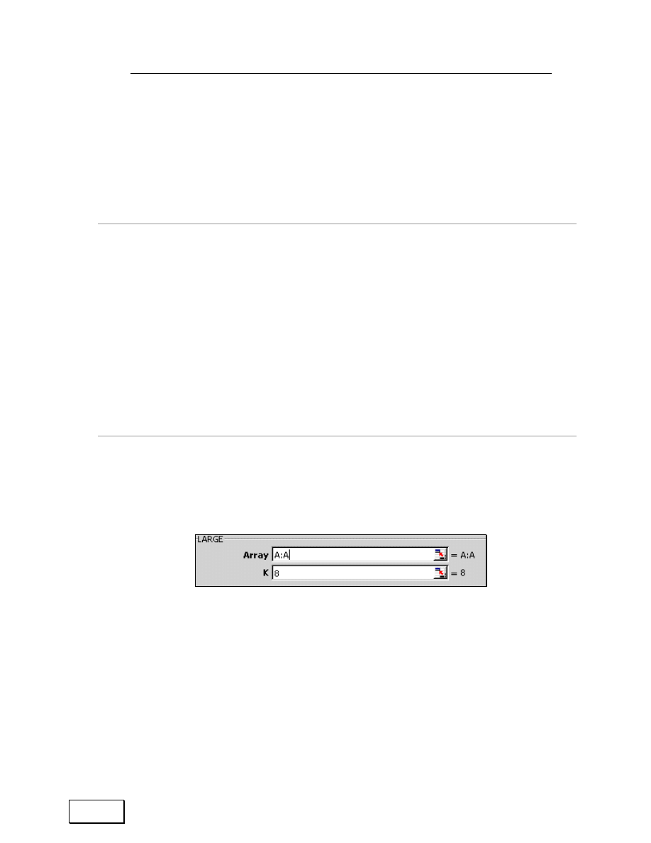
Chapter 6: Functions for Basic Statistics
97
Menu path to function: STATISTICAL/MAX , & STATISTICAL/MAXA.
Data Requirements: Any array/range with real numbers. In addition,
MAXA may include
“
True,”
“
False,” or numbers in text format
MIN (“Minimum value”)
MIN and MINA: The functions calculate the smallest value in a series
Menu path to function: STATISTICAL/MIN, & STATISTICAL/MINA
Data Requirements: Any array/range with real numbers. In addition,
MINA include
“
True,”
“
False,” or numbers in text format
LARGE
This function calculates the K
th
largest value in a range.
Figure 92: LARGE
Menu path to function: STATISTICAL/LARGE
Data Requirements: Any real number.
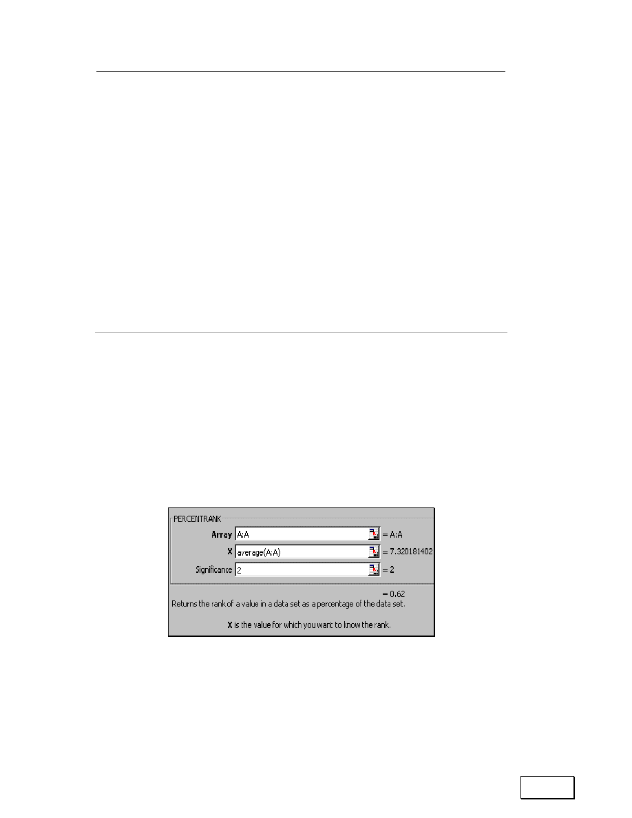
Statistical Analysis with Excel
98
SMALL
This function calculates the Kth smallest value in a range.
Menu path to function: STATISTICAL/SMALL
Data Requirements: Any real number.
6.3.D
RANK OR RELATIVE STANDING OF EACH CELL WITHIN THE
RANGE OF A SERIES
PERCENTRANK
The PERCENTRANK function returns the rank of a value in a data set as
a percentage of the data set. The function can be used to evaluate the
relative standing of a value within a data set. For example, you can use
PERCENTRANK to evaluate the standing of a test score among all scores
for the test.
Figure 93: Percentrank of the average/mean
Menu path to function: INSERT/FUNCTION / STATISTICAL /
PERCENTRANK.

Chapter 6: Functions for Basic Statistics
99
Data requirements: Any array/range with real numbers.
RANK
The function RANK calculates the relative rank of a value within a series
of numbers data. You can choose to obtain the ranks on the basis of
ascending or descending values. X is the data point whose rank is desired
within the range. Order sets the sorting direction— 1 for ascending
ranking, 0 or blank for descending ranking. Cells with the same value
cells are given the same rank.
Menu path to function: INSERT / FUNCTION / STATISTICAL / RANK.
Data requirements: Any array/range with real numbers.
6.4
MEASURES OF DISPERSION (STANDARD
DEVIATION & VARIANCE)
Table 12: Standard Deviation & Variance.
Function
Description
Location within
INSERT /
FUNCTION
Data Requirements
Sample
dispersion:
STDEV, VAR
The functions STDEV
and VAR estimate the
sample standard
deviation and variance,
respectively. VAR is
the square of STDEV.
STATISTICAL /
STDEVA
&
STATISTICAL /
VARA
Any range with
sufficient number of
numeric data points.
Text and logical values
are excluded.
STDEVA, VARA These are variants of
the functions above but
STATISTICAL /
Text and logical values
such as TRUE and

Statistical Analysis with Excel
100
Function
Description
Location within
INSERT /
FUNCTION
Data Requirements
with a wider range of
acceptable data types
as input data.
STDEVA
&
STATISTICAL /
VARA
FALSE are included in
the calculation. TRUE
is valued as 1; text or
FALSE is valued as 0.
Population
dispersion:
STDEVP,
VARP
The less often used
population dispersion
functions are
sometimes also used
for large sample sizes.
STDEVP assumes that
its data are the entire
population. Typically,
you use the sample
formulae. For large
sample sizes, STDEV
and STDEVP return
approximately equal
values. VARP is
square of STDEVP
STATISTICAL /
STDEVA
&
STATISTICAL /
VARA
A large number of
observations.
Text and logical values
are excluded.
STDEVPA,
VARPA
These are variants of
the functions above but
with a wider range of
acceptable data types
as input data
STATISTICAL /
STDEVA
&
STATISTICAL /
VARA
Text and logical values
such as TRUE and
FALSE are included in
the calculation. TRUE
is valued as 1; text or
FALSE is valued as 0.
Text and logical values
such as TRUE and
FALSE are included in
the calculation. TRUE
is valued as 1; text or
FALSE is valued as 0.
Figure 94: Dialog for STDEV

Chapter 6: Functions for Basic Statistics
101
Figure 95: Dialog for STDEVA. Note that the functions with the “A” suffix request “Values”
as input while the equivalent non–suffixed functions request “Numbers”
6.5
SHAPE ATTRIBUTES OF THE DENSITY FUNCTION
(SKEWNESS, KURTOSIS)
6.5.A
SKEWNESS
Skewness measures asymmetry around the mean. The parameter is best
interpreted as relative to the Normal Density Function (whose Skewness
equals zero). The interpretation of the Skewness for a series (relative to
the Normal Density Function) is:
— Skewness > 0 Æ asymmetric tail with more values above the mean.
— Skewness < 0 Æ asymmetric tail with more values below the mean.
The next three figures shown Density Functions that have a Skewness >
0, = 0, and < 0, respectively, for three variables Y1, Y2 and Y3. (Y2 is
distributed Normally).
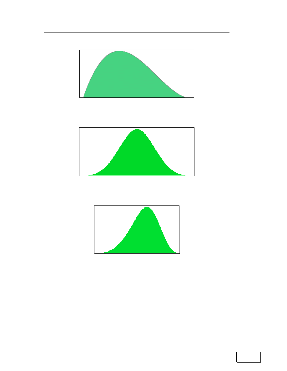
Statistical Analysis with Excel
102
Figure 96: Distribution of series Y1.
Skewness > 0
Figure 97: Distribution of series Y2.
Skewness = 0.
Figure 98: Distribution of series Y3
Skewness < 0
Samples will be available at
http://www.vjbooks.net/excel/samples.htm
.
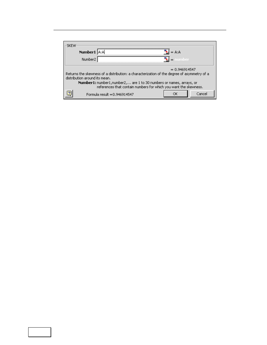
Chapter 6: Functions for Basic Statistics
103
Figure 99: SKEW (Skewness)
Menu path to function: INSERT / FUNCTION / STATISTICAL / SKEW
6.5.B
KURTOSIS
Compared with the Normal Density Function (which has a Kurtosis of
zero), the interpretation of the kurtosis for a series is:
— Kurtosis > 0Æ peaked relative to the Normal Density Function
— Kurtosis < 0Æ flat relative to the Normal Density Function
The next figure shows three Density Functions. The Density Functions
lie around the same Mean and Median, but note the difference in the
relative flatness of the Density Functions:
Distribution of series X1 is the flattest with a Kurtosis < 0, that of X2 is
less flat with a Kurtosis = 0 (a Normal Density Function) and that of
series X3 is the least flat with a Kurtosis > 0.
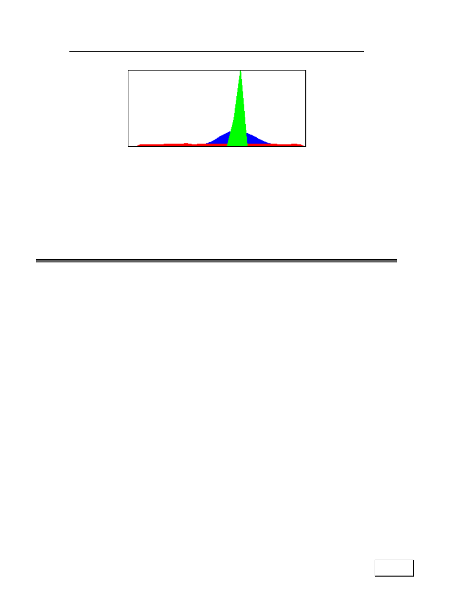
Statistical Analysis with Excel
104
Figure 100: Example of Density Functions with different Skewness
Samples will be available at
http://www.vjbooks.net/excel/samples.htm
.
Menu path to function: INSERT / FUNCTION / STATISTICAL / KURT
6.6
FUNCTIONS ENDING WITH AN “A” SUFFIX
These functions calculates the same statistic as their
“
twin” formula (the
one without the prefix
“
A”) but include a wider range of valid cell values
in the relevant formula. The
“
A” –suffixed functions include the following
types of cell values:
— Logical (and not numeric) like
“
True” and
“
False” (valued as 1 and 0,
respectively),
— Blank cells (valued as 0), and
— Text (valued as 0).
A text string or a blank cell is valued as zero. The next table lists these
twin functions:

Chapter 6: Functions for Basic Statistics
105
Table 13: Functions ending with the “A” suffix.
The non–
prefixed
function
The
“
A” prefixed
“
twin” formula
Comment
AVERAGE
AVERAGEA
Simple average/mean
COUNT
COUNTA
Count of valid cells. The prefixed
function is very useful in counting.
STDEV
STDEVA
Standard deviation
STDEVP
STDEVPA
Standard deviation from a population or
a very large sample (relative to
population)
VAR
VARA
Variance
VARP
VARPA
Variance from population (and not
sample) data, or from a very large
sample (relative to population)
MIN
MINA
Minimum value
MAX
MAXA
Maximum value

Statistical Analysis with Excel
106

Page for Notes

Statistical Analysis with Excel
108
CHAPTER 7
PROBABILITY DENSITY FUNCTIONS AND
CONFIDENCE INTERVALS
This chapter teaches the following topics
— PROBABILITY DENSITY FUNCTION (PDF)
— CUMULATIVE DENSITY FUNCTION (CDF)
— THE CDF AND CONFIDENCE INTERVALS
— INVERSE MAPPING FUNCTIONS
— NORMAL DENSITY FUNCTION
— STANDARD NORMAL OR Z–DENSITY FUNCTION
— T–DENSITY FUNCTION
— F–DENSITY FUNCTION
— CHI-SQUARE DENSITY FUNCTION
— OTHER CONTINUOUS DENSITY FUNCTIONS: BETA, GAMMA,
EXPONENTIAL, POISSON, WEIBULL & FISHER
— DISCRETE PROBABILITIES— BINOMIAL, HYPERGEOMETRIC
& NEGATIVE BINOMIAL
— LIST OF DENSITY FUNCTION FUNCTIONS — PROBABILITY
DENSITY FUNCTION (PDF), CUMULATIVE DENSITY
FUNCTION (CDF)
— LIST OF SELECT INVERSE FUNCTION
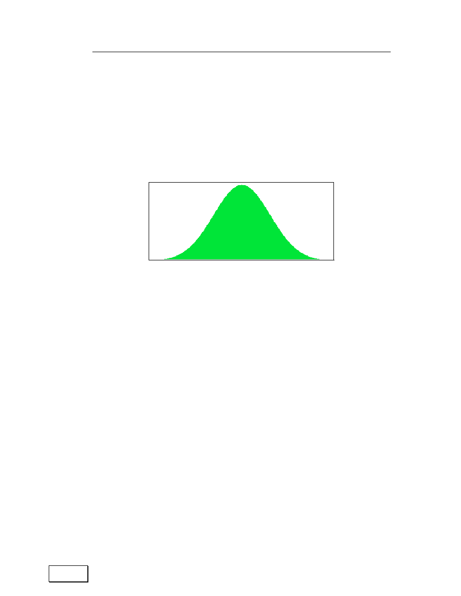
Chapter 7: Probabiity Density Functions & Confidence Intervals
109
7.1
PROBABILITY DENSITY FUNCTIONS (PDF),
CUMULATIVE DENSITY FUNCTIONS (CDF), AND
INVERSE FUNCTIONS
7.1.A
PROBABILITY DENSITY FUNCTION (PDF)
Figure 101: Probability Density Function (PDF)
The horizontal axis contains the values of the series/series. The vertical
height of the curve at a point on the X–axis shows the probability
associated (or frequency) with that point. (The total area under the curve
equals 1; so, all the
“
heights” add up to 1 or 100 %.) The higher the
frequency with which that point is observed in a series/series, the higher
is its frequency.
An often–used probability Density Function — the
“
Normal” probability
Density Function — is shown in the previous figure. This Density
Function has some convenient properties:
— its Mean, Mode and Median are the same
— it does not have a left or right skew, and
— the left half is a mirror image of the right half.
All these
“
symmetrical” properties allow one to draw inferences from tests
run on series that are distributed
“
Normally.”

Statistical Analysis with Excel
110
Based on several theorems, postulate,
“
most data series start behaving
more and more like a series that follows a Normal Density Function as
the sample size (or number of data points) increases.” (This presumption
follows from the
“
Central Limit Theorem.”) This has made the Normal
Density Function the bedrock of most statistics and econometrics.
7.1.B
CUMULATIVE DENSITY FUNCTION (CDF)
We are typically interested in measuring the area under the curve (a) to
the left of an X value (b) to the right of an X value, or (c) between two X
values. The height of the curve at any X value is not so useful by itself
because it does not answer any of these questions directly.
A better graphical tool to measure the
“
area under the curve” is the
Cumulative Density Function (CDF). A CDF plots the X categories
against the
“
probability of a value taking a value below the chosen X
value.”
The CDF for the Normal Density Function is reproduced in the next
figure. The curve increases from left to right (from 0 to 1
8
). The height at
any X-value tells us
“
the probability of a value having a value below this
X-value equals the Y-axis value of the CDF at this X.”
8
The area under any Density Function curve always equals 1. The relative
frequency equals (frequency that X takes on this particular value) divided by (the
total sample size). Therefore, in a sense, the height gives the frequency weight for
each X value. If you sum all the relative frequencies, their sum is “sample size
divided by sample size” equals 1. This is the area under the curve. It can also be
expressed in percentage terms; the total percentage area then becomes 100%.
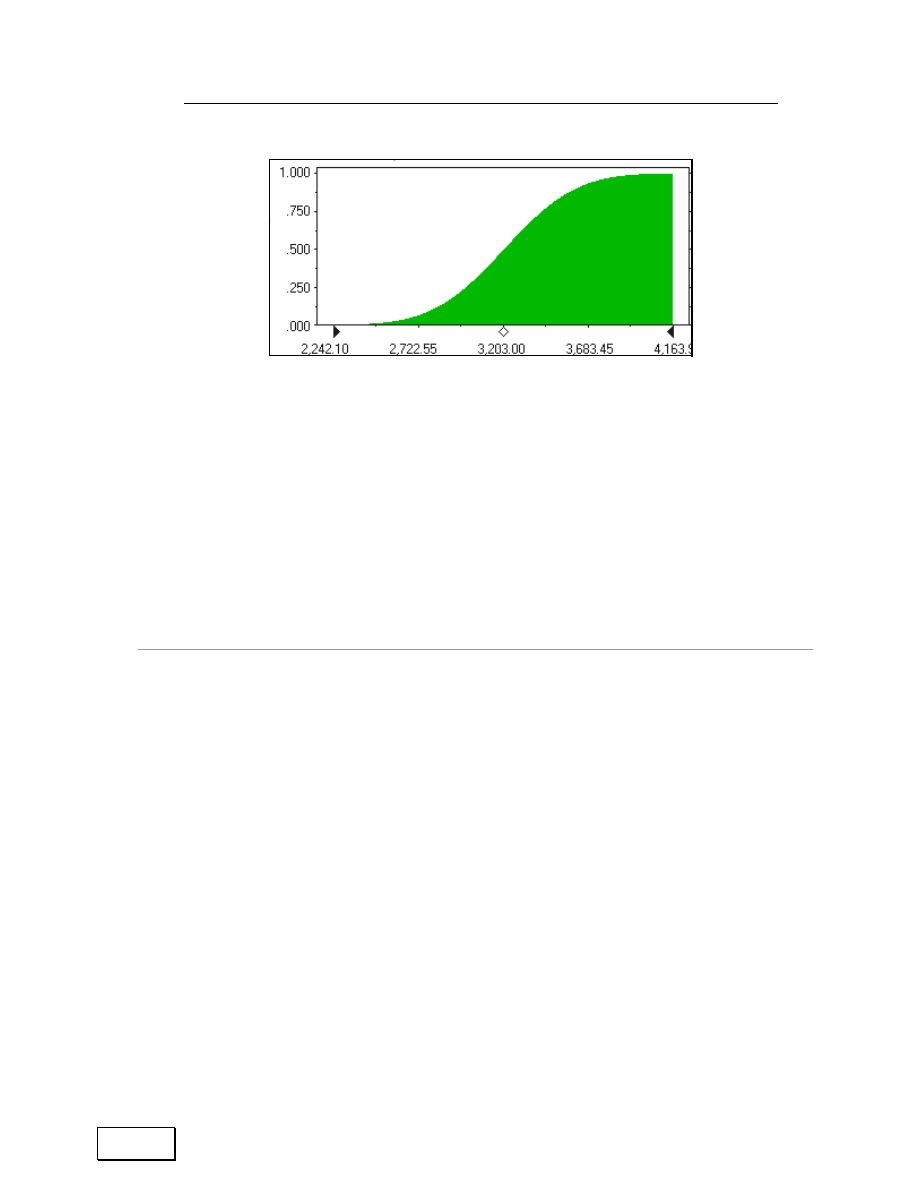
Chapter 7: Probabiity Density Functions & Confidence Intervals
111
Figure 102: The “Cumulative Density Function” (CDF) associated with the Probability
Density Function (PDF) shown in the previous figure
The CDF is a better tool for answering the typical questions about the
properties of a data series. CDF is of great importance for building
Confidence Intervals and implementing hypothesis tests.
In fact, for some Density Functions, Excel only measures the CDF only
(and not the CDF & PDF).
The CDF and Confidence Intervals
The concept of a Confidence Interval for a measured parameter (typically
for a mean) is based on the concept of probability depicted by a Density
Function curve. A Confidence Interval of 95% is a range of X values
within whose range the sum of the relative frequencies is 0.95 or 95%.
I will use this property to show how to create Confidence Intervals for
various distributions using the Inverse of the CDF. (You will learn more
on the Inverse in the next sub-section.)

Statistical Analysis with Excel
112
Table 14: Probability Density Function (PDF) and Cumulative Density Function (CDF)
Cumulative Density Function (CDF) &
Probability Density Function (PDF):
Information requirements for
parameterization
Function
Is there an option
to request the
Cumulative
Density Function
(CDF)?
Mean
Std
Dev
Degrees of
freedom
Other
TDIST
9
Tails #
LOGNORMDIST
9
9
9
FDIST
9
2
nd
degree of
freedom
BETADIST
alpha, beta, upper and
lower bound
CHIDIST
9
NORMDIST
9
9
9
NORMSDIST
9
WEIBULL
Alpha and
beta
NEGBINOMDIST
(Probability)
# of
successes
BINOMDIST
9
(Probability)
EXPONDIST
9
Lambda
GAMMADIST
9
Alpha and
beta
HYPGEOMDIST
Sample size, population size, # of
successes in population
POISSON
9
9
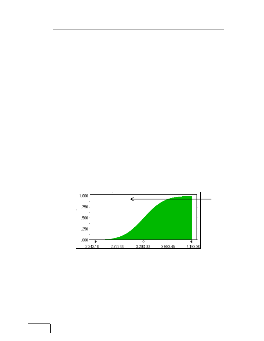
Chapter 7: Probabiity Density Functions & Confidence Intervals
113
7.1.C
INVERSE MAPPING FUNCTIONS
The Cumulative Density Function (CDF) tells us “For any X series, the
probability of the value of X falling below a specific x value can be
calculated from the height of the Cumulative Density Function (CDF)
at that x value.”
An inverse function does the reverse mapping:
“
For a probability P, the X
to who’s left the probability of the data lying can be obtained by a reverse
reading of the Cumulative Density Function (CDF). That is, from
“
Desired Cumulative Probability Æ unknown X that will give this desired
cumulative probability P.”
Alternatively,
“
Inverse” functions find the X value that corresponds to a
certain
“
probability of values below the X equaling a known cumulative
probability.”
Figure 103: Reading inverse mapping from a Cumulative Density Function (CDF). The
arrows show the values below which are 95% of the values of the data series.
Inverse functions permit easy construction of Confidence intervals.
This will be shown several times in further sections whenever I discuss
the construction of Confidence intervals.
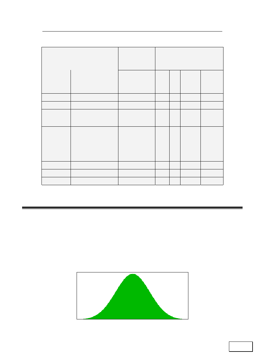
Statistical Analysis with Excel
114
Table 15: Inverse functions (also used to create Confidence intervals). Samples will be
available at http://www.vjbooks.net/excel/samples.htm.
Information
required by all
inverse
functions
Other information
requirements
Function
Inverse Function
(
“
probability to
value”) of this
Cumulative Density
Function (CDF)?
Probability for
which the
corresponding
value is sought
Mean
Std
Dev
Degrees
of
freedom
Other
TINV
TDIST
9
9
LOGINV
LOGNORMDIST
9
9
9
FINV
FDIST
9
9
Second
degree of
freedom
BETAINV
BETADIST
9
alpha,
beta,
upper
and
lower
bound
CHIINV
CHIDIST
9
9
NORMINV
NORMDIST
9
9
9
NORMSINV
NORMSDIST
9
7.2
NORMAL DENSITY FUNCTION
The Normal Density Function has several properties that make it easy to
make generalized inferences for the attributes of a series whose Density
Function can be said to be
“
Normal.”
Figure 104: A Normal Probability Density Function
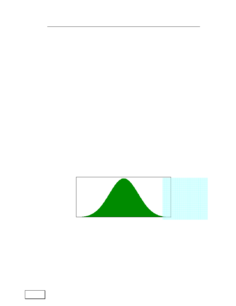
Chapter 7: Probabiity Density Functions & Confidence Intervals
115
Symmetry
The major measures of central tendency — the mean, median, and mode
— all lie at the same point right at the place where the bell shaped curve
is at its greatest height.
The Density Function is perfectly symmetrical around this
“
confluence” of
central tendencies. Therefore, the left half of the Density Function
(measured as all points to the left of the mode/median/mean) is a mirror
image of the right half of the Density Function.
This is shown in the next figure — the lighter shaded half is a mirror
image of the darker shaded half. So, the frequency of the values of the
variables becomes lower (that is, the height of the curve lowers) as you
move away from the mode/mean/median towards either extreme. This
change is gradual and occurs at the same rate for negative and positive
deviations from the mean.
Figure 105: An idealized “symmetrical” Normal Density Function. Note that the relatively
lightly shaded half is a mirror image of the relatively darker shaded half
The symmetry also implies that:
(a) The Density Function is not
“
skewed” to the left or right of the
mode/median/mean (and, thus, the Skewness measure = 0)
(b) The Density Function is not
“
too” peaked (which would imply that the

Statistical Analysis with Excel
116
change in probability is very rapid when moving from the
mode/median/mean towards an extreme) nor
“
too” flat (which
would imply that the change in probability is very slow when
moving from the mode/median/mean towards an extreme).
The first property implies that Skewness = 0, and the second
implies that Kurtosis = 0.
Convenience of using the Normal Density Function
If a series is Normally distributed, then you just need two parameters for
defining the Density Function for any series X— the mean and standard
deviation of the variables values! This is because, once you know the
mean, you also know the mode and median (as these two statistics equal
the mean for a Normal Density Function).
Once you know the standard deviation, you know the spread of values
around the mean/mode/median. (A series that follows a Normal Density
Function is not skewed to the left or right, nor is
“
too” peaked or
“
too”
flat.)
Are all large-sample series Normally Distributed?
Some formal mathematical theorems and proofs support the theory that
“
as the sample size gets larger most Density Functions become more like
the Normal Density Function.” Therefore, for example, if a series has a
left skewed Density Function when a sample of 20 observations is used, it
may also behave more like a symmetrical (that is, a zero–skewed) Normal
Density Function if the sample size is, for example, 1000 observations.
(Even if the Density Function does not have the classic bell–shape of a

Chapter 7: Probabiity Density Functions & Confidence Intervals
117
normal curve, it can behave like a Normal Density Function if it satisfies
— to a sufficient extent — the conditions that imply normality –
• The fact that the mode, mean and median are very close to each
other
• An additional feature is that the Density Function is roughly
symmetrical around the mode/median/mean.
Statistics & Econometrics: Dependence of Methodologies on the
assumption of Normality
Assuming that variables are distributed Normally is a practice that
underlies— and even permits— most hypothesis testing in econometrics
and statistics. Without this assumption, statistics, as we know it, would
lose much of its power to estimate coefficients and establish relationships
amongst variables.
Assume you have three variables — X1, X2, and X3. X1 is measured in
dollars with a mean of $2.30, X2 also in dollars with a mean of $30,000
and X3 in tons. You assume that all the variables are distributed
Normally. This permits you to make inferences about the series. Once
you know the mean and standard deviation for X1, you can make
statements like
“
60% of the values of X1 lie below $2.62,”
“
Between the
values $24,000 and $28,000, we will find that 18% of the values of X2 will
lie,” or,
“
Over 40% of the values of X3 lie below 24 tons.” (Note: the
figures are chosen arbitrarily). This is fine. But the problem is that the
relation between the
“
mean, standard deviation, X values and probability”
must be calculated anew for each of the variables because they are
measured in different units (dollars versus tons) or/and on different
scales and ranges (X1 versus X2 in our example).

Statistical Analysis with Excel
118
This limits the usefulness of using the Normal Density Function to assess
the relation between series values and the probability of values occurring
less than, equal to or above them. In practical terms, you would need a
statistics textbook that lays out the relationship between an X value and
probability for all possible combinations of mean and standard deviation!
The Standard Normal and its power
Luckily, a method removes the need for such exhaustive table listings.
This method involves rescaling all series that follows a Normal Density
Functions to a common scale such that, on the new scale, the variables
have a mean/mode/median of zero and a standard deviation of one. The
process is called
“
standardization” and this standardized Density
Function is called the standard Normal Density Function or the Z –
Density Function.
The Z –scores are also used to standardize the Density Functions of the
means of variables or the estimates of statistical coefficients. If the
standard error of mean for the population from which the sample is
unknown (as is typically the case), then the T Density Function is used
instead of the Z Density Function.
7.2.A
THE PROBABILITY DENSITY FUNCTION (PDF) AND
CUMULATIVE DENSITY FUNCTION (CDF)
PDF:
NORMDIST (x, mean, standard deviation, false) Æ probability of values
taking the value X
CDF:
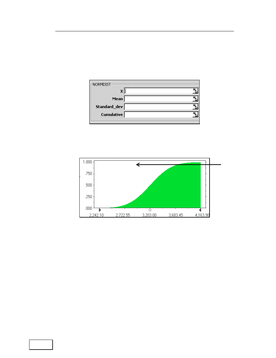
Chapter 7: Probabiity Density Functions & Confidence Intervals
119
NORMDIST (x, mean, standard deviation, true) Æ probability of values
lying to the left of X
Figure 106: The dialog for estimating the probability associated with a value of a point in a
series that follows a Normal Density Function
Figure 107: The Cumulative Density Function (CDF) for a series that follows a Normal
Density Function. The arrows show the value to the left of which lie 95% of the values in the
Density Function.
The Cumulative Density Function (CDF) is the integral of the function on
the right hand side in the above equation. The range of integration is
negative infinity (or the population minimum) to the X value being
studied.
Menu path to function: INSERT / FUNCTION / STATISTICAL /
NORMDIST.
Data requirements: The data series should follow the assumed Density
Function type (Normal).
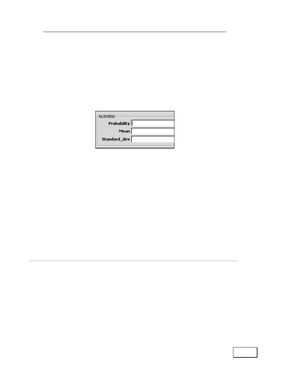
Statistical Analysis with Excel
120
7.2.B
INVERSE FUNCTION
This function calculates the inverse of the normal cumulative Density
Function for a user–specified mean and standard deviation.
NORMINV (probability below the X, MEAN, STANDARD DEVIATION) Æ X
Figure 108: The inverse function for a Normal Density Function
7.2.C
CONFIDENCE INTERVALS
Menu path to function: INSERT / FUNCTION / STATISTICAL /
NORMINV.
Data requirements: The data series should follow the assumed Density
Function type (Normal).
95% Confidence Interval
The Confidence Interval contains all but 2.5% of the extreme values on
each of the tails of the Density Function (Probability Density Function
(PDF)) or is the value that corresponds to 0.025 and 0.975 on the
Cumulative Density Function (CDF). The 95% Confidence Interval for a
series that follows a Normal Density Function with mean =
µ and
standard deviation =
σ is defined by the results of the two inverse

Chapter 7: Probabiity Density Functions & Confidence Intervals
121
functions at these two probabilities:
— NORMINV (0.025, mean, standard deviation)
— NORMINV (0.975, mean, standard deviation) for the lower and
upper limit
90% Confidence Interval
The 90% Confidence Interval for a series that follows a Normal Density
Function with mean =
µ and standard deviation = σ is defined by the
results of the two inverse functions at these two probabilities:
— NORMINV (0.05, mean, standard deviation)
— NORMINV (0.95, mean, standard deviation) for the lower and
upper limit
Table 16: Normal Density Function— Formulae for 90%, 95%, and 99% Confidence limits.
Confidence
level
Formula for lower bound
Formula for upper bound
90%
NORMINV (0.05, mean,
standard deviation)
9
NORMINV (0.95, mean,
standard deviation)
95%
NORMINV (0.025, mean,
standard deviation)
NORMINV (0.975, mean,
standard deviation)
9
Note that many books use the following symbols or phrases for the mean and standard
deviation”
• µ or “mu” for mean
• σ or “sigma standard deviation/error
• σ
2
or “sigma square variance
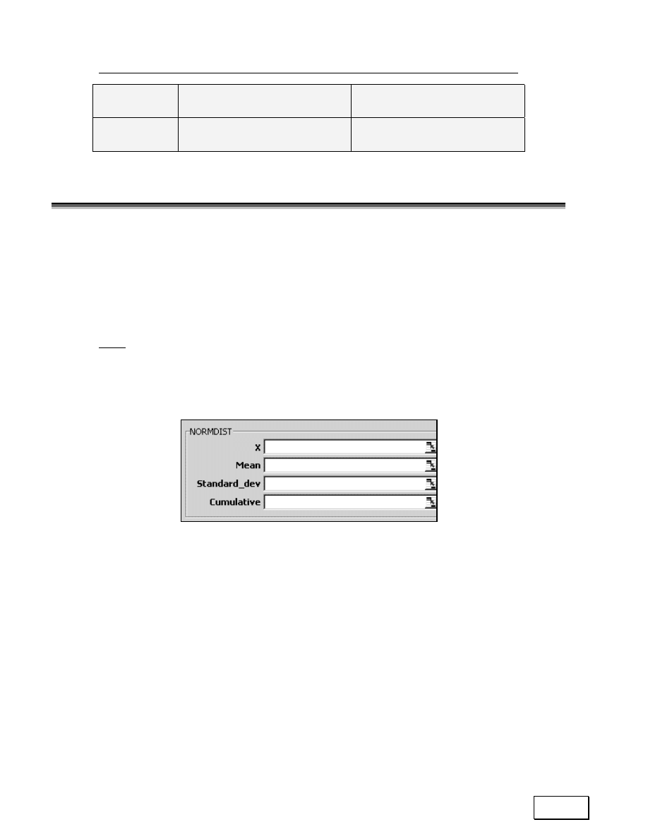
Statistical Analysis with Excel
122
Confidence
level
Formula for lower bound
Formula for upper bound
99%
NORMINV (0.005, mean,
standard deviation)
NORMINV (0.995, mean,
standard deviation)
7.3
STANDARD NORMAL OR Z–DENSITY FUNCTION
The Cumulative Density Function (CDF) is the integral of the function on
the right hand side in the above equation. The range of integration is
negative infinity to the Z value being studied.
CDF:
NORMSDIST (z) Æ probability of values lying to the left of Z
Figure 109: The Normal Density Function
Menu path to function: INSERT / FUNCTION / STATISTICAL
/NORMSDIST.
Data requirements: The data series ‘z’ should follow the assumed Density
Function type (Standard Normal).
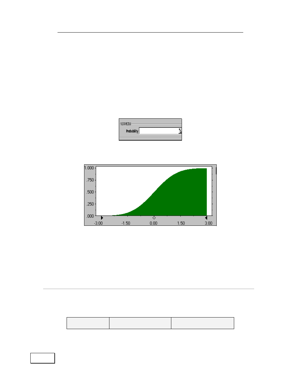
Chapter 7: Probabiity Density Functions & Confidence Intervals
123
Inverse function
This function calculates the inverse of the Standard Normal CDF. The
inverse function for a Standard Normal Density Function requires only
one parameter.
NORMSINV (probability below the X) Æ X
Figure 110: NORMSINV
Figure 111: The cumulative Standard Normal Density Function (or the Probit)
Menu path to function: INSERT / FUNCTION / STATISTICAL /
NORMSINV. Data requirements: The data series ‘z’ should follow the
assumed Density Function type (Standard Normal).
Confidence Intervals
Table 17: Standard Normal Density Function: Formulae for 90%, 95% and 99% Confidence
limits.
Confidence level Formula for lower bound Formula for upper bound
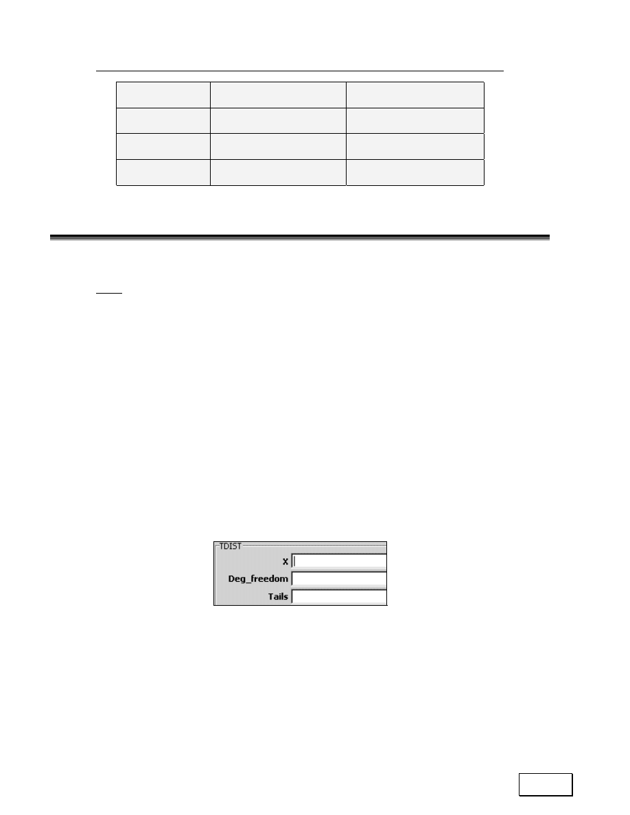
Statistical Analysis with Excel
124
Confidence level Formula for lower bound Formula for upper bound
90%
NORMSINV (0.05)
NORMSINV (0.95)
95%
NORMSINV (0.025)
NORMSINV (0.975)
99%
NORMSINV (0.005)
NORMSINV (0.995)
7.4
T–DENSITY FUNCTION
CDF:
TDIST (x, degrees of freedom, tails) Æ probability of values lying to the
left of X
In the box Tails, specify the number of tails to return.
• If tails = 1, TDIST returns the one–tailed Density Function.
• If tails = 2, TDIST returns the two–tailed Density Function.
For example, TDIST (1.96, 60, 2) equals 0.054645, or 5.46 percent
Figure 112: T–Distribution
Menu path to function: INSERT /FUNCTION /STATISTICAL /TDIST.
Data Requirements: The data series should follow the T Density Function.
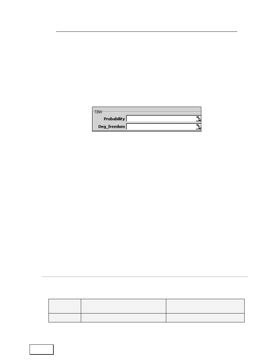
Chapter 7: Probabiity Density Functions & Confidence Intervals
125
Inverse function
This function calculates the t–value of the Student's t–Density Function
as a function of the probability and the degrees of freedom.
TINV (probability below the X, degrees of freedom) Æ X
Figure 113: The inverse function for a T–Density Function
A one–tailed t–value can be returned by replacing probability with
2*probability. For a probability of 0.05 and degrees of freedom of 10, the
two–tailed value is calculated with T (0.05, 10), which returns 2.28139.
The one–tailed value for the same probability and degrees of freedom can
be calculated with T (2*0.05, 10), which returns 1.812462.
TINV (0.054645, 60) equals 1.96
Menu path to function: INSERT /FUNCTION /STATISTICAL /TINV.
Data requirements: The data series should follow the assumed Density
Function type (T).
Confidence Intervals
Table 18: T Density Function— Formulae for 90%, 95%, and 99% Confidence limits (2 tails).
Confidence
level
Formula for lower bound
Formula for upper bound
90%
TINV (0.05, degrees of freedom)
TINV (0.95, degrees of freedom)

Statistical Analysis with Excel
126
Confidence
level
Formula for lower bound
Formula for upper bound
95%
TINV (0.025, degrees of freedom) TINV (0.975, degrees of freedom)
99%
TINV (0.005, degrees of freedom) TINV (0.995, degrees of freedom)
7.4.A
ONE–TAILED CONFIDENCE INTERVALS
95% Confidence Interval
A 95 % Confidence Interval contains all but 5% of the extreme values on
one–tail of the Density Function (Probability Density Function (PDF)) or
is the value that corresponds to 0.05 or 0.95 on the Cumulative Density
Function (CDF) (the former for the left tail of 5% and the latter for a right
tail of 5%).
The 95% Confidence Interval for a T–distributed series is defined by the
results of the two inverse functions at this probability:
Left tail:
Negative infinity to TINV (0.05, degrees of freedom).
Right tail:
TINV(0.95, degrees of freedom) to positive infinity.
Note:
TINV(0.05, degrees of freedom) = –TINV(0.95, degrees of freedom)
90% Confidence Interval
A 90 % Confidence Interval contains all but 10% of the extreme values on
one–tail of the Density Function (Probability Density Function (PDF)) or

Chapter 7: Probabiity Density Functions & Confidence Intervals
127
is the value that corresponds to 0.1 or 0.9 on the Cumulative Density
Function (CDF) (the former for the left tail of 10% and the latter for a
right tail of 10%).
The 90% Confidence Interval for a T–distributed series is defined by the
results of the two inverse functions at this probability:
• Left tail: Negative infinity to TINV (0.1, degrees of freedom).
• Right tail: TINV (0.9, degrees of freedom) to positive infinity.
Note:
TINV(0.1, degrees of freedom) = –TINV(0.9, degrees of freedom)
Table 19: T Density Function— Formulae for 90%, 95%, and 99% Confidence limits (right tail
only).
Confidence
level
Formula for lower left-tail Confidence upper limit (the lower
limit equals negative infinity)
90%
TINV (0.9, degrees of freedom)
95%
TINV (0.95, degrees of freedom)
99%
TINV (0.99, degrees of freedom)
Table 20: T Density Function— Formulae for 90%, 95%, and 99% Confidence limits (left tail
only)
Confidence
level
Formula for right-tail Confidence lower limit (the upper limit
equals positive infinity)
90%
–TINV (0.1, degrees of freedom)
95%
–TINV (0.05, degrees of freedom)
99%
–TINV (0.01, degrees of freedom)
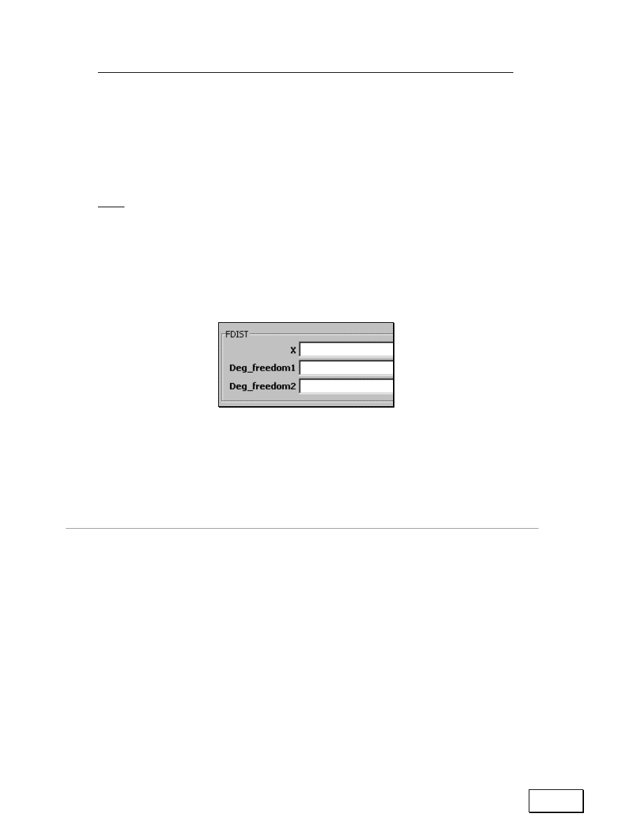
Statistical Analysis with Excel
128
7.5
F–DENSITY FUNCTION
The F test is used for testing model significance and other joint hypothesis
in ANOVA, Regression Analysis, etc.
CDF:
FDIST (x, numerator degrees of freedom, denominator degrees of freedom)
Menu path to function: INSERT / FUNCTION / STATISTICAL / FDIST.
Figure 114: F–Distribution
Data requirements: The data series should follow the assumed Density
Function type (F).
Inverse function
FINV (probability below the X, numerator degrees of freedom, denominator
degrees of freedom) Æ X
Menu path to function: INSERT / FUNCTION / STATISTICAL /FINV.
Data requirements: The data series should follow the F Density Function.

Chapter 7: Probabiity Density Functions & Confidence Intervals
129
Figure 115: The inverse function for an F–Density Function
One–tailed Confidence Intervals
Table 21: F Density Function— Formulae for 90%, 95%, and 99% Confidence Intervals (right
tail only).
Confidence
level
Formula for upper One-tail Confidence lower limit (the upper limit equals
positive infinity)
90%
FINV (0.9, numerator degrees of freedom, denominator degrees of freedom)
95%
FINV (0.95, numerator degrees of freedom, denominator degrees of freedom)
99%
FINV (0.99, numerator degrees of freedom, denominator degrees of freedom)
7.6
CHI-SQUARE DENSITY FUNCTION
The Chi-square test is used for testing model significance and other joint
hypothesis in Maximum Likelihood estimation, Logit, Probit, etc.
The one–tailed probability of the Chi-Square Density Function: CDF:
CHIDIST (x, degrees of freedom) Æ probability of values lying to the left of X
Figure 116: CHI-Square Density Function

Statistical Analysis with Excel
130
Menu path to function: INSERT /FUNCTION /STATISTICAL /CHIDIST.
Data requirements: The data series should follow the assumed Density
Function type (Chi-Square).
Inverse function
CHIINV (probability, degrees of freedom) Æ X
Menu path to function: INSERT /FUNCTION /STATISTICAL /CHIINV.
Data requirements: The data series should follow the Chi-Square Density
Function.
Figure 117: CHIINV
One–tailed Confidence Intervals
Table 22: Chi-Square Density Function: Formulae for 90%, 95%, and 99% Confidence limits
(right tail only). Samples will be available at http://www.vjbooks.net/excel/samples.htm.
Confidence
level
Formula for upper One-tail Confidence lower limit (the upper
limit equals positive infinity)
90%
CHIINV (0.9, degrees of freedom)
95%
CHIINV (0.95, degrees of freedom)
99%
CHIINV (0.99, degrees of freedom)

Chapter 7: Probabiity Density Functions & Confidence Intervals
131
7.7
OTHER CONTINUOUS DENSITY FUNCTIONS: BETA,
GAMMA, EXPONENTIAL, POISSON, WEIBULL &
FISHER
7.7.A
BETA DENSITY FUNCTION
CDF:
BETADIST (x, alpha, beta, lower bound A, upper bound B) Æ probability of
values lying to the left of X
Menu path to function: INSERT / FUNCTION / STATISTICAL /
BETADIST.
Data requirements: The data series should follow the Beta Density
Function.
Figure 118: BETA Density Function
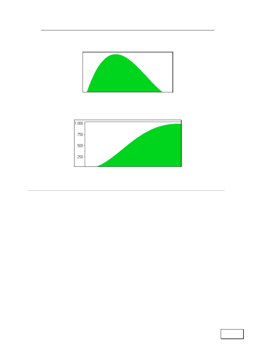
Statistical Analysis with Excel
132
Figure 119: Note how the Density Function Probability Density Function (PDF) is skewed to
one side and has a less sharp “hill” at top — compared to a Normal Probability Density
Function (PDF)
Figure 120: The Cumulative Density Function (CDF) shows (on the Y –Axis) the proportion of
values that lie below a certain X value of the series
Inverse Function
BETAINV (probability, alpha, beta, lower bound A, upper bound B) Æ X
Menu path to function: INSERT / FUNCTION / STATISTICAL /
BETAINV.
Data requirements: The data series should follow the assumed Density
Function type (Beta).
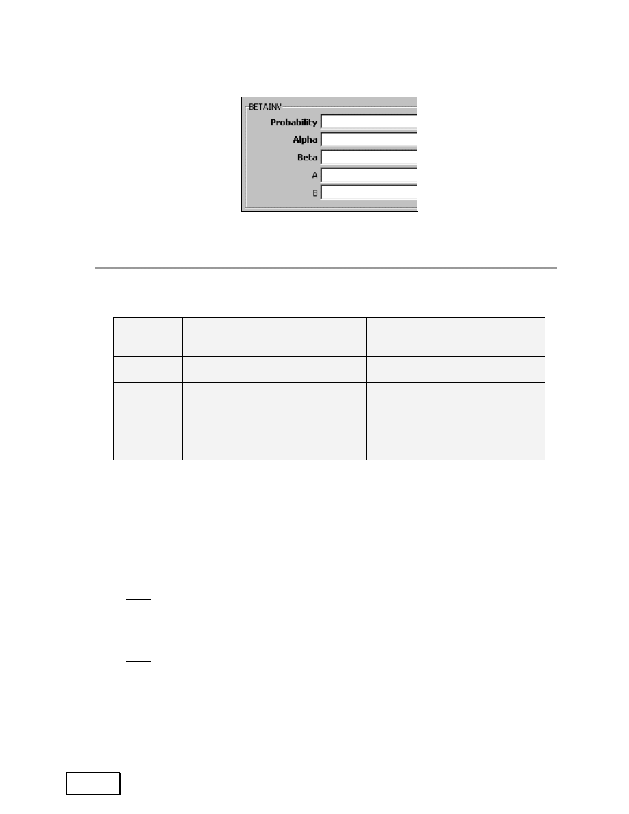
Chapter 7: Probabiity Density Functions & Confidence Intervals
133
Figure 121: The inverse function for a BETA Density Function
Confidence Intervals
Table 23: BETA Density Function— Formulae for 90%, 95%, and 99% Confidence limits.
Confidence
level
Formula for lower bound
Formula for upper bound
90%
BETAINV (0.05, alpha, beta, A, B) BETAINV (0.95, alpha, beta, A, B)
95%
BETAINV (0.025, alpha, beta, A, B) BETAINV (0.975, alpha, beta, A,
B)
99%
BETAINV (0.005, alpha, beta, A, B) BETAINV (0.995, alpha, beta, A,
B)
7.7.B
GAMMA DENSITY FUNCTION
The Gamma Density Function is commonly used in queuing analysis.
CDF:
GAMMADIST (x, Alpha, Beta, true) Æ probability of values lying to the left of X)
PDF:
GAMMADIST (x, Alpha, Beta, false) Æ probability of values taking the value X)
Menu path to function: INSERT /FUNCTION /STATISTICAL
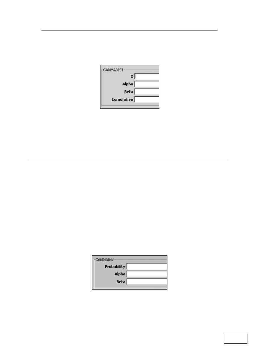
Statistical Analysis with Excel
134
/GAMMADIST.
Figure 122: GAMMA Density Function
Data requirements: The data series should follow the assumed Density
Function type (Gamma).
Inverse Function
GAMMAINV (probability below the X, alpha, beta) Æ X
Menu path to function: INSERT /FUNCTION /STATISTICAL
/GAMMAINV.
Data requirements: The data series should follow the assumed Density
Function type (Gamma).
Figure 123: The inverse function for a GAMMA Density Function

Chapter 7: Probabiity Density Functions & Confidence Intervals
135
Confidence Intervals
Table 24: Gamma Density Function: Formulae for 90%, 95% and 99% Confidence limits.
Samples will be available at http://www.vjbooks.net/excel/samples.htm.
Confidence
level
Formula for lower bound
Formula for upper bound
90%
GAMMAINV (0.05, alpha, beta) GAMMAINV (0.95, alpha, beta)
95%
GAMMAINV (0.025, alpha, beta)
GAMMAINV (0.975, alpha,
beta)
99
GAMMAINV 0005, alpha, beta
GAMMAINV 0995, alpha, beta
If an inverse function does not converge after 100 iterations, the function
returns the #N/A error value.
7.7.C
EXPONENTIAL DENSITY FUNCTION
PDF:
EXPONDIST (x, lambda, False) Æ probability of values taking the value X
CDF:
EXPONDIST (x, lambda, True) Æ probability of values lying to the left of X
Menu path to function: INSERT /FUNCTION /STATISTICAL
/EXPONDIST.
Data requirements: The data series should follow the Exponential Density
Function.
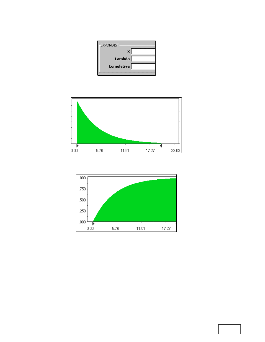
Statistical Analysis with Excel
136
Figure 124: Dialog for the Exponential Distribution
Figure 125: Exponential Probability Density Function (PDF)
Figure 126: Exponential Cumulative Density Function (CDF)
EXPONDIST (0.2, 10, TRUE) equals 0.864665 while EXPONDIST (0.2, 10,
FALSE) equals 1.353353
Further detail is beyond the scope of this book.

Chapter 7: Probabiity Density Functions & Confidence Intervals
137
7.7.D
FISHER DENSITY FUNCTION
This topic is beyond the scope of this book.
7.7.E
POISSON DENSITY FUNCTION
This Density Function is used for predicting the number of events ‘X’
occurring over a specific time.
PDF:
POISSON (x, expected value, false) Æ probability of values taking the value X
CDF:
POISSON (x, expected value, true) Æ probability of values lying to the left of X
Further detail is beyond the scope of this book.
7.7.F
WEIBULL DENSITY FUNCTION
PDF:
WEIBULL (x, a, b, false) Æ probability of values taking the value X
CDF:
WEIBULL (x, a, b, true) Æ probability of values lying to the left of X
Further detail is beyond the scope of this book.

Statistical Analysis with Excel
138
7.7.G
DISCRETE PROBABILITIES— BINOMIAL, HYPERGEOMETRIC &
NEGATIVE BINOMIAL
This topic is beyond the scope and aim of this book.
Binomial Density Function
This function is used to ascertain the probability of obtaining a
“
head” in a
coin toss. X can take only two discrete values. Further detail is beyond
the scope of this book.
Hypergeometric Density Function
The Density Function captures event probabilities in problems of
sampling without replacement. The sample is taken from a discrete finite
population like a deck of cards. Further detail is beyond the scope of this
book.
Negative Binomial
This function measures the probability of
“
number of coin tosses before
first or K
th
heads (in a coin toss).”

Chapter 7: Probabiity Density Functions & Confidence Intervals
139
7.8
LIST OF DENSITY FUNCTION
Table 25: PDF and CDF functions
Information
required by
all functions
Other information requirements
Function
Is there a
function that
does the
converse of
this mapping
and, if so, the
name of the
function?
Is there an
option to
request the
cumulative
probability?
Value (s)
for which
the
probability
is being
sought
Mean
Std Dev
Deg
ree
s o
f free
do
m
Ot
her
TDIST
TINV
9
9
LOGNORMDIST
LOGINV
9
9
9
9
FDIST
FINV
9
9
2
nd
degree
of freedom
BETADIST
BETAINV
9
alpha, beta, upper and lower
bound
CHIDIST
CHIINV
9
9
NORMDIST
NORMINV
9
9
9
9
NORMSDIST
NORMSINV
9
9
WEIBULL
9
alpha,
beta
NEGBINOMDIST
—
# of failures
(Probability)
# of
successes
BINOMDIST
—
9
# of
successes
(Probability)
EXPONDIST
—
9
9
Lambda
GAMMADIST
GAMMAINV
9
9
alpha,
beta
HYPGEOMDIST
—
# of
successes
in sample
Sample & population size, # of
successes in population
POISSON
—
9
9
9

Statistical Analysis with Excel
140
7.9
SOME INVERSE FUNCTION
Table 26: Inverse Functions
Information
required by all
inverse
functions
Other information
requirements
Function
Inverse mapping
(
“
probability to
value”) of which
cumulative
probability
function?
Probability for
which the
corresponding
value is sought
Mean
Std
Dev
Degrees
of
freedom
Other
TINV
TDIST
9
9
LOGINV
LOGNORMDIST
9
9
9
FINV
FDIST
9
9
2
nd
degree
of
freedom
BETAINV
BETADIST
9
alpha, beta, Upper and
lower bound
CHIINV
CHIDIST
9
9
NORMINV
NORMDIST
9
9
9
NORMSINV
NORMSDIST
9

Chapter 7: Probabiity Density Functions & Confidence Intervals
141

Page for Notes

Chapter 8: Other Mathematics & Statistics Functions
143
CHAPTER 8
OTHER MATHEMATICS & STATISTICS FUNCTIONS
This chapter briefly displays some other functions available in Excel. The
topics in this chapter are:
— COUNTING AND SUMMING
— COUNT, COUNTA
— COUNTBLANK
— COMPARING COUNT, COUNTA AND COUNTBLANK
— SUM
— PRODUCT
— SUMPRODUCT
— THE “IF “COUNTING AND SUMMING FUNCTIONS
— SUMIF
— COUNTIF
— TRANSFORMATIONS (LIKE LOG, EXPONENTIAL, ABSOLUTE,
ETC)
— STANDARDIZING A SERIES THAT FOLLOWS A NORMAL
DENSITY FUNCTION
— DEVIATIONS FROM THE MEAN
— CROSS SERIES RELATIONS
— COVARIANCE AND CORRELATION FUNCTIONS
— SUM OF THE SUM OF THE SQUARES OF TWO VARIABLES

Statistical Analysis with Excel
144
— SUM OF THE SQUARES OF DIFFERENCES ACROSS TWO
VARIABLES
— SUM OF THE DIFFERENCE OF THE SQUARES OF TWO
VARIABLES
8.1
COUNTING AND SUMMING
COUNT function
This function counts the number of valid cells in a range. Cells are valid
only if there value is numeric or a date.
Menu path to function: INSERT / FUNCTION / STATISTICAL
/ COUNT.
Data requirements: Numbers and dates are included in the count. Not
counted cells include those that contain error values, text, blank cells, and
logical values (like TRUE and FALSE). The X values can be input as
references to one or more ranges that may be non–adjacent.
The second range can be referenced in the first text-box
“
Value1” after
placing a comma after the first range, or it could be referenced in the
second text-box
“
Value2.”
If you use the second text-box, then a third text-box
“
Value3” will
automatically open. (As you fill the last visible box, another box opens
until the maximum number of boxes — 30 — is reached.)
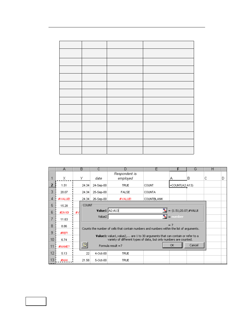
Chapter 8: Other Mathematics & Statistics Functions
145
Table 27: Sample data for the “Count” functions.
The example is in the sample file “Count.xls.”
A
B
C
D
Y
Date
Respondent is employed
.51
24.34
24— Sep— 2000
TRUE
20.07
24.34
25— Sep— 2000
FALSE
VALUE!
24.34
26— Sep— 2000
#VALUE!
15.28
24.34
27— Sep— 2000
FALSE
DIV/0!
#VALUE!
28— Sep— 2000
TRUE
11.63
24.34
29— Sep— 2000
#N/A!
.86
30— Sep— 2000
TRUE
REF!
22.00
1— Oct— 2000
FALSE
.74
22.00
TRUE
NAME?
22.00
3— Oct— 2000
.13
22.00
4— Oct— 2000
TRUE
N/A!
21.58
5— Oct— 2000
TRUE
Figure 127: COUNT
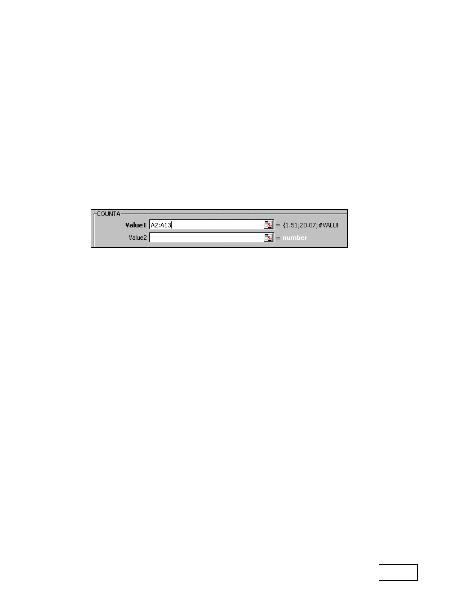
Statistical Analysis with Excel
146
COUNTA function also counts cells with logical or text values
This function counts the number of valid cells in a range. Valid values
include cells with numeric, date, text, logical, or error value.
COUNTA
only excludes empty cells, but text and logical values are only counted if
you type them directly into the list of arguments are counted. If an
argument is a data array or range reference, only numbers in that data
array or range reference.
Figure 128: The function COUNTA is a variant of the COUNT function. The example is in the
sample file “Count.xls.”
Menu path to function: INSERT / FUNCTION / STATISTICAL /
COUNTA.
Data requirements: Unlike the COUNT function, COUNTA will include
the label row in the count. (So, if you have one label in the referenced
range, you may want to use
“
= COUNTA (A:A) — 1”.) The X values can be
input as references to one or more ranges that may be non–adjacent. The
second range can be referenced in the first text-box
“
Value1” after placing
a comma after the first range, or it could be referenced in the second text-
box
“
Value2.” If you use the second text-box, then a third text-box
“
Value3” will automatically open. (As you fill the last visible box, another
box opens until the maximum number of boxes — 30 — is reached.) The
function does not count invalid cell values when counting the number of X
values.
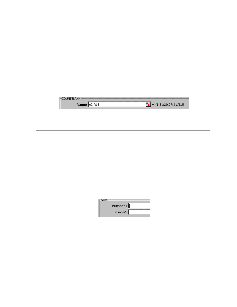
Chapter 8: Other Mathematics & Statistics Functions
147
COUNTBLANK function counts the number of empty cells in the range
reference
This function counts the number of blank cells in a range.
Menu path to function: INSERT /FUNCTION
/INFORMATION/COUNTBLANK.
Figure 129: COUNTBLANK. The example is in the sample file “Count.xls.”
SUM function
This function sums the values in the data array.
SUM = X
1
+ X
2
+…. +X
n
Menu path to function: INSERT / FUNCTION / MATH / SUM.
Figure 130: SUM
Data requirements: This function does not include blank cells or cells with
values that are of the following formats: text, and logical values (that is,
TRUE and FALSE.)
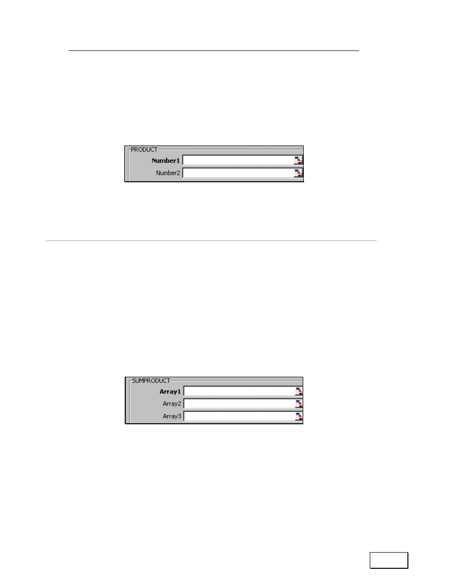
Statistical Analysis with Excel
148
PRODUCT function
This function multiplies all the values referenced.
PRODUCT = X
1
* X
2
*….* X
n
Figure 131: PRODUCT (multiplying all the values in a range)
Menu path to function: INSERT / FUNCTION / MATH / PRODUCT.
SUMPRODUCT function
This function multiplies corresponding components in two or more data
arrays/ranges, and then sums the results of these multiplications. The
data arrays/ranges must have the same number of data points.
Menu path to function: INSERT /FUNCTION /MATH /SUMPRODUCT
Figure 132: SUMPRODUCT (multiplying individual data points across data series and then
adding up the results of all these multiplications).
Data Array1, data Array2, data Array3 ... are 2 to 30 data arrays/ranges
whose components you desire to multiply and then add. The minimum
number of arrays is two. The data arrays must have the same number of
data points. Non-numeric cell values are assigned the value of zero.

Chapter 8: Other Mathematics & Statistics Functions
149
The X values can be input as references to two or more ranges that may
be non–adjacent. The second range should be referenced in the second
text-box
“
Array2.” If you use the third text-box, then a fourth text-box
“
Array4” will automatically open. (As you fill the last visible box, another
box opens until the maximum number of boxes — 30 — is reached.)
Example
The following formula multiplies all the components of the two data
arrays on the preceding worksheet and then adds the products— that is,
3*2 + 4*7 + 8*6 + 6*7 + 1*5 + 9*3.
Note:
Samples will be available at
http://www.vjbooks.net/excel/samples.htm
.
8.2
THE “IF” COUNTING AND SUMMING FUNCTIONS:
STATISTICAL FUNCTIONS WITH LOGICAL
CONDITIONS
I display two
“
if-then” two-step functions in this section. The functions
first evaluate a criterion. If a cell in the referenced range satisfies the
criteria then the second part of the function includes this cell.
SUMIF function
This function adds the values in a range if the cell with the value satisfies
a user-defined criterion.
•
In the box Range, enter a reference to the range of cells you want
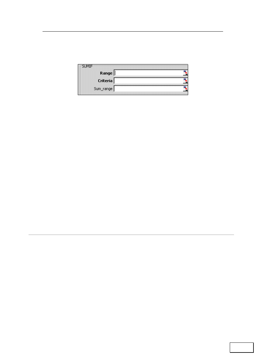
Statistical Analysis with Excel
150
evaluated.
Figure 133: SUMIF (summing only the cells whose value satisfies one “if” condition)
• In the box Criteria, enter the condition (a number, expression, or
text) that defines which cells values will be summed. For
example, Criteria can be expressed as 32,
“
32,”
“
>32”.
• In the box Sum_range, you may reference the actual cells to sum.
The cells in sum range are summed only if their corresponding
cells in the entire Range match the criteria. If sum range is
omitted, all the
“
criterion-satisfying” cells in the Range are
summed.
Menu path to function: INSERT / FUNCTION / MATH / SUMIF. The
Criteria should be relevant to the type of data/text in the queried range.
COUNTIF function
This function counts the number of cells in a range that satisfy a user-
defined criterion.
The dialog for
“
COUNTIF
“
requires two inputs from the user. The
“
Range” is similar to the functions shown previously. The
“
Criteria” is a
logical condition set by you.
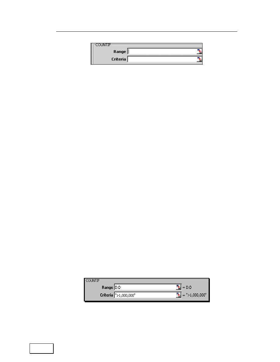
Chapter 8: Other Mathematics & Statistics Functions
151
Figure 134: COUNTIF (counting only the cells whose value satisfies one “if” condition)
• In the box Range, enter a reference to the range of cells you seek to
evaluate.
• In the box Criteria, enter the condition (a number, expression, or
text) that defines which cells will be counted. For example,
Criteria can be expressed as 32,
“
32,”
“
>32,”
“
tea.”
Menu path to function: INSERT /FUNCTION /STATISTICAL /COUNTIF.
Data requirements: The range can take any values. The Criteria should
be relevant to the type of data/text in the queried range.
Example
Choose the range
“
D:D” and the condition
“
>1,000,000”. The function is
“
Count the number of cases in the range D:D, but only if the value of the
cell is greater than 1 million.”
For a pictorial reproduction of this, see the next figure.
Figure 135: Entering the data input and logical criterion
Execute the dialog by clicking on the button OK. The formula is written

Statistical Analysis with Excel
152
onto the cell. The next figure illustrates this. Depress the ENTER key.
Figure 136: The function as written into the cell
8.3
TRANSFORMATIONS (LOG, EXPONENTIAL,
ABSOLUTE, SUM, ETC)
Table 28: Common transformation functions
Function
Description
Location within
INSERT
/FUNCTION
Data Requirements
Sign
This function outputs the
sign of a number.
Returns 1 if the number
is positive, zero (0) if the
number is 0, and –1 if
the number is negative.
Useful for red–flagging
data, or using in
functions like IF,
COUNTIF, SUMIF and
CHOOSE.
MATH /SIGN
Any real value.
Absolute
number
ABS = | X |
MATH /ABS
One real number.
Square root
The square root of a
number.
MATH/SQRT
One positive real
number.

Chapter 8: Other Mathematics & Statistics Functions
153
Function
Description
Location within
INSERT
/FUNCTION
Data Requirements
Y = X
1/2
Log natural
LN (X)
This function calculates the
natural logarithm of a
number. Natural
logarithms are based on
the constant e (2.718).
LN (85) = 4.454347.
This mean:
“
If you raise the
base e to the power of 4.45
you will get 85. Æ LN (85)
= 4.45.
Conversely,
exp (4.45) = e^ (4.45) =
2.718^ (4.45) = 85.
MATH /LN
One positive real
number.
Exponential
This function calculates the
exponential to a number.
MATH /EXP
One positive real
number.
Log to the
base 10
LOG10 (X)
This function calculates the
base 10 logarithm of a
number.
LOG10 (85) = 1.934
because the base of 10
needs to be raised 1.934
times to get 85:
10
1.934
= 85
LOG10 (10) = 1 because
10
1
= 10
LOG10 (1000) = 3 because
10
3
= 1000
MATH /LOG10
One positive real
number.

Statistical Analysis with Excel
154
Function
Description
Location within
INSERT
/FUNCTION
Data Requirements
Log to a user
defined base
This function calculates the
logarithm of a number to
the base you specify. The
default base is 10. For
natural log use base e =
2.718.
LOG (X, base)
LOG (100) = 2 Æ base 10.
(Since 10
2
= 100).
LOG (27, 3) = 3 Æ base 3.
(Since 3
3
= 27).
LOG (86, 2.7182818) = 4.45
Æ
same as natural log.
Because— (exp (4.45) = 85).
MATH/LOG.
A positive real
number X and the
(optional) base of
the logarithm.
If base is omitted,
it is assumed = 10.
Standardizing a series that follows a Normal Density Function
Converts a value in a series X to its equivalent standard normal
transformation.
STANDARDIZE (x, AVERAGE (X), STDEV (X)) where X is all the numbers
in the X data series.
Menu path to function:
INSERT/FUNCTION/STATISTICAL/STANDARDIZE.
Data requirement: The function requires three input numbers: x, mean of
the X series, and the standard deviation of the X series. The mean and
standard deviation can be written as a
“
function within a function.”
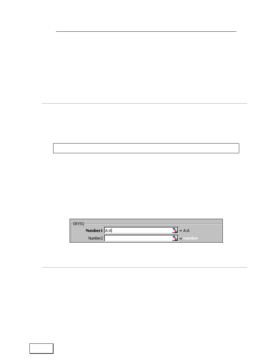
Chapter 8: Other Mathematics & Statistics Functions
155
8.4
DEVIATIONS FROM THE MEAN
The formulas in this and the next section provide estimates of functions
used in formulas for parameters obtained in advanced analysis like
ANOVA, Correlation, Regression, etc.
DEVSQ
This function calculates the sum of squares of deviations of data points
from their sample mean
Σ ((x — mean (x))
2
Menu path to function: MATH/DEVSQ
Data Requirements: A range(s) of real numbers, inclusive of zero.
Figure 137: Summation of the squares of the “differences of individual points from the mean of
the series”
AVEDEV
This function calculates the average of the absolute deviations of data
points from their mean. AVEDEV is a measure of the variability in a data
set.

Statistical Analysis with Excel
156
Menu path to function: STATISTICAL/AVEDEV
Menu path to function: A range(s) of real numbers, inclusive of zero.
8.5
CROSS SERIES RELATIONS
8.5.A
COVARIANCE AND CORRELATION FUNCTIONS
The functions are CORREL, COVAR, PEARSON, & RSQ. I recommend
using the Analysis ToolPak Add-In — refer to 10.3.
8.5.B
SUM OF SQUARES
SUMX2PY2 function evaluates the “Sum of the sum of the squares of each
case in two variables”
This function estimates the summation of the squares of individual points
in two series.
Σ (x
2
+ y
2
)
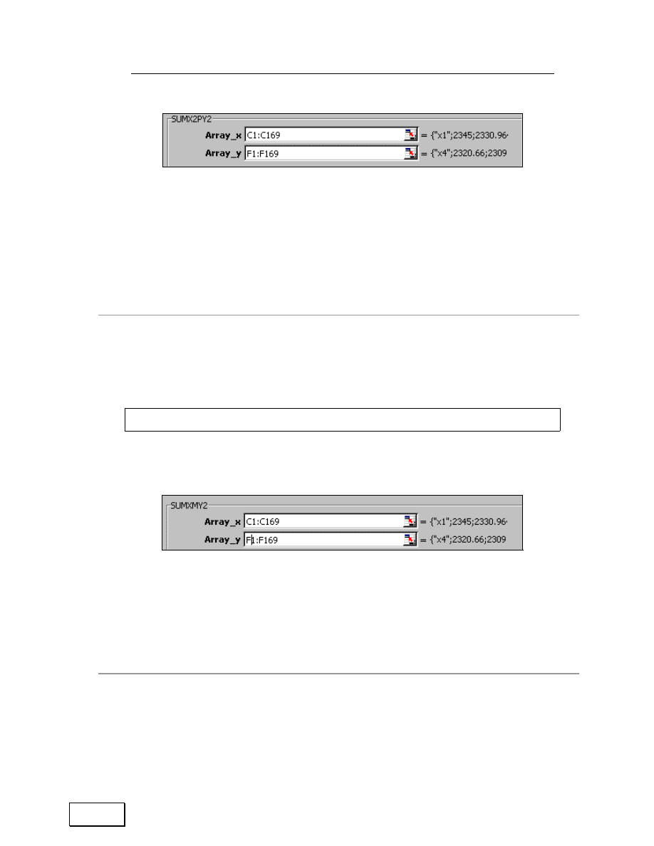
Chapter 8: Other Mathematics & Statistics Functions
157
Figure 138: Summation of the squares of individual points in two series. Samples will be
available at http://www.vjbooks.net/excel/samples.htm.
Menu path to function: INSERT/FUNCTION/MATH/SUMX2PY2.
Data requirements: This function needs two data series.
SUMXMY2 function
This function estimates Sum of the squares of differences of each case in
two across two variables.
Σ ((x — y)
2
)
Figure 139: Summation of the squares of the “differences in individual points in two series.”
Samples will be available at http://www.vjbooks.net/excel/samples.htm.
Menu path to function: INSERT/FUNCTION/MATH/SUMXMY2. Data
requirements: This function needs two data series.
SUMX2MY2 function
This function estimates the Sum of the difference of the squares of each
case in two variables.

Statistical Analysis with Excel
158
Σ (x
2
— y
2
)
Menu path to function: INSERT/FUNCTION/MATH/SUMX2MY2.
Data requirements: This function needs two data series.

Page for Notes

Statistical Analysis with Excel
160
CHAPTER 9
ADD-INS: ENHANCING EXCEL
This chapter discusses the following topics:
— WHAT CAN AN ADD-IN DO?
— WHY USE AN ADD-IN (AND NOT JUST EXCEL
MACROS/PROGRAMS)?
— ADD–INS INSTALLED WITH EXCEL
— OTHER ADD-INS
— THE STATISTICS ADD-IN
— CHOOSING THE ADD-INS
9.1
ADD-INS: INTRODUCTION
An
“
Add-In” is a software application that adds new functionality to
Excel. The Add-In typically seamlessly fits into the Excel interface,
providing accessibility to its functionality through
— new menus
— new options in existing menus
— new functions

Chapter 9: Add-ins: Enhancing Excel
161
— new toolbars and specific toolbar icons
9.1.A
WHAT CAN AN ADD-IN DO?
Almost anything an imaginative software developer could create.
Usually, an Add-In provides functionality that is useful for a particular
type of analysis/industry — statistics, finance, real estate, etc.
9.1.B
WHY USE AN ADD-IN?
The Add-In could have its base code written in software languages like C,
C++, FORTRAN, Pascal, etc. This is important because some algorithms
and operations (like simulations) operate best when written in a specific
language. Therefore, the developer uses the best language/tool to create
the functionality and then packages this inside an Add-In.
9.2
ADD–INS INSTALLED WITH EXCEL
Some Add–Ins are available in the Microsoft Office CD–ROM and are
installed (but not activated
10
) along with Excel. I show the use of three
Add–ins.
10
Figure 540 and Figure 542 show how to activate the Add-ins

Statistical Analysis with Excel
162
9.3
OTHER ADD-INS
Many commercially sold Add-Ins can be almost like separate software just
needing Excel as the
“
host.” Two examples:
— Crystal Ball
risk analysis software
— UNISTAT
software for conducting advanced statistics and
econometrics from inside Excel
Hundreds of software companies construct Add-Ins. The greatest
contribution of this book, if I succeed in doing so, would be the opening of
this massive potential functionality to Excel users.
9.4
THE STATISTICS ADD-IN
The Analysis ToolPak Add-In that ships with Excel can conduct several
procedures including descriptives, regression, ANOVA, F-test, correlation,
T-tests, moving average, and histogram. Let us learn how to use this
“
Add-In.”
9.4.A
CHOOSING THE ADD-INS
Choose the menu option TOOLS/ADD-INS. You will see several Add-Ins
as shown in Figure 140. (You may not see all the Add–Ins shown in the
next two figures.)
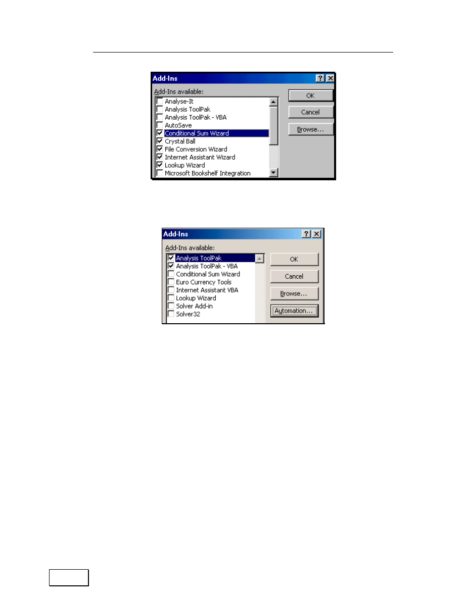
Chapter 9: Add-ins: Enhancing Excel
163
Figure 140: Selecting an Add-In
Figure 141: In Excel XP, the Add-Ins dialog provides access to “Automation.” This topic is
beyond the scope of this book.
You need the
“
Analysis ToolPak Add-Ins.” Select — by clicking on it —
the box to the left of these Add-Ins (shown in Figure 142). Execute the
dialog by clicking on the button OK and wait for some time while the Add-
Ins are
“
loaded” or
“
registered” with Excel. An Add-In has to be
loaded/registered before it is available for use. The Add-In remains
loaded across sessions. It is only
“
unloaded” when you select the option

Statistical Analysis with Excel
164
TOOLS/ADD-INS and deselect the Add-In
11
.
Figure 142: The Add-In pair for data analysis
You have activated the
“
Analysis ToolPak.” At the bottom of the menu
TOOLS, you will see the option
“
DATA ANALYSIS the bottom— this
option was not there before you accessed the Add-In. (This is illustrated
in Figure 143.)
The statistical procedures are accessed through this new option.
Note:
Usually Add-Ins expose their functionality by creating new menu
options or even new menus. The menu option
“
Data analysis”
provides the statistics functionality available in
“
Analysis ToolPak”
and
“
Analysis ToolPak VB.” The menu options
“
Optquest” down till
CB Bootstrap” are linked to the Add-in
“
Crystal Ball” (not shipped in
the Office CD-ROM).
11
If too many Add-Ins are loaded, Excel may work too slowly, or even freeze. If you find
this problem occurring, then just load the Add-in when you are going to use it and
unload it before quitting Excel.
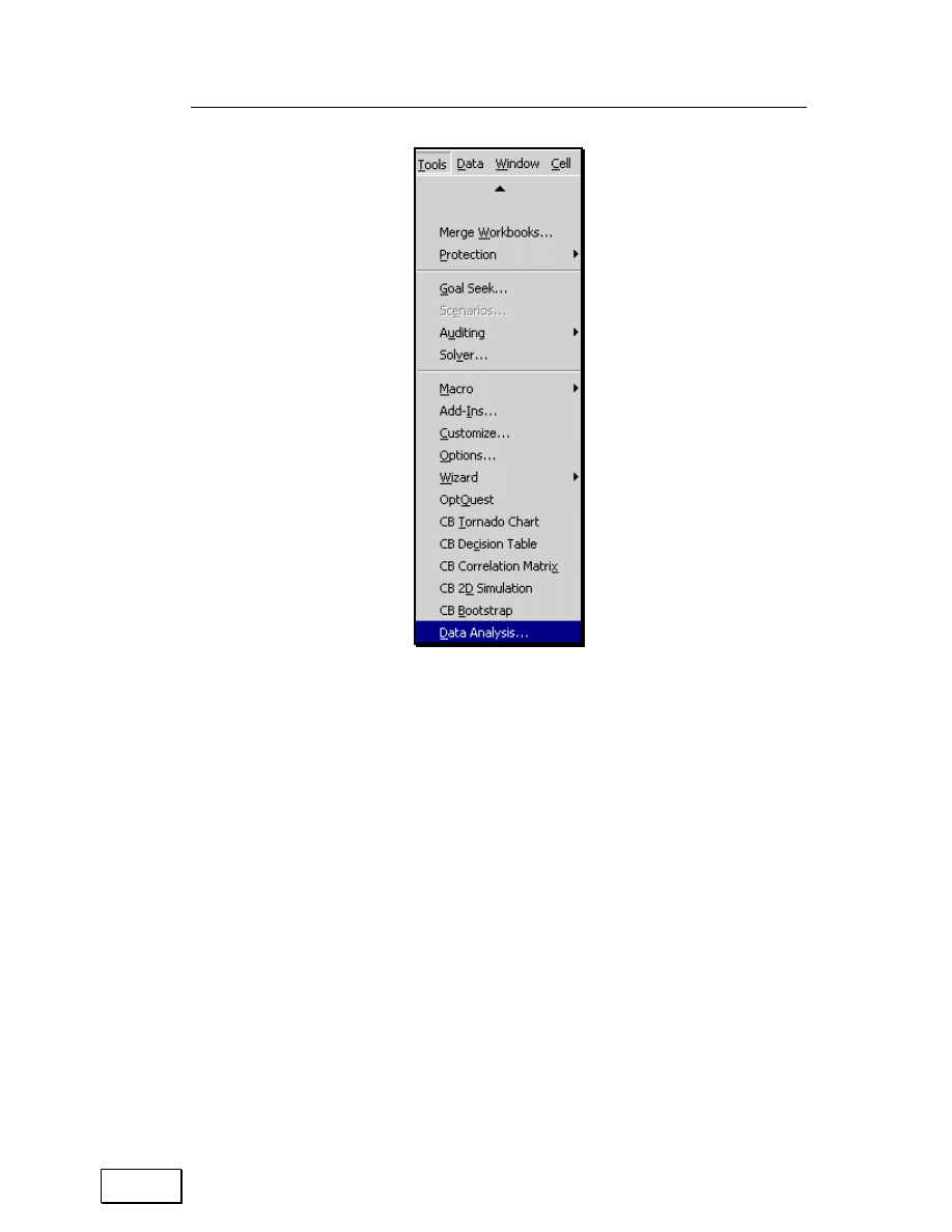
Chapter 9: Add-ins: Enhancing Excel
165
Figure 143: The “Data Analysis” menu option

Statistical Analysis with Excel
166

Page for Notes

Statistical Analysis with Excel
168
CHAPTER 10
STATISTICS TOOLS
This chapter discusses the following topics:
— DESCRIPTIVE STATISTICS
— RANK AND PERCENTILE
— BIVARIATE RELATIONS— CORRELATION, COVARIANCE
A proper analysis of data must begin with an analysis of the statistical
attributes of each series in isolation — univariate analysis. From such an
analysis, you can learn:
— How the values of a series are distributed — normal, binomial,
etc.
— The central tendency of the values of a series (mean, median,
and mode)
— Dispersion of the values (standard deviation, variance, range,
and quartiles)
— Presence of outliers (extreme values)

Chapter 10: Statistics Tools
169
The answer to these questions illuminates and motivates further, more
complex, analysis. Moreover, failure to conduct univariate analysis may
restrict the usefulness of further procedures (like correlation and
regression). Reason: even if improper/incomplete univariate analysis may
not directly hinder the conducting of more complex procedures, the
interpretation of output from the latter will become difficult (because you
will not have an adequate understanding of how each series behaves).
Note: I do not go into the details of each statistics procedure. For such
details, refer to your statistics textbook or to “SPSS for Beginners”
(available at http://www.vjbooks.net and amazon.com).
This chapter requires the Analysis ToolPak Add-Ins; chapter 9 shows how
to learn how to launch the Add-Ins.
10.1
DESCRIPTIVE STATISTICS
I do not supply the sample data for most of the examples in chapters 36-40.
My experience is that many readers glaze over the examples and do not go
through the difficult step of drawing inferences from a result if the sample
data results are the same as those in the examples in the book.
Choose the menu option TOOLS/DATA ANALYSIS
12
. The dialog shown
in Figure 144 opens.
12
If you do not see this option, then use TOOLS / ADD-INS to activate the Add-In for
data analysis. Refer to section 41.4.
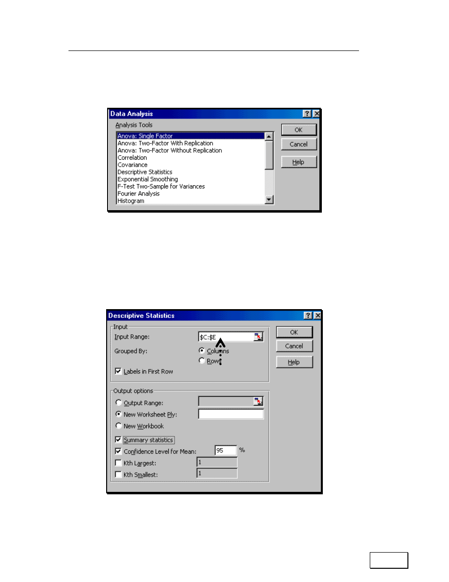
Statistical Analysis with Excel
170
Figure 144: The options for the menu TOOLS/DATA ANALYSIS
Choose the statistical procedure “Descriptive Statistics.” The dialog for
“Descriptive Statistics” opens. Figure 145 shows this dialog (user-input
form).
Figure 145: Descriptive Statistics dialog

Chapter 10: Statistics Tools
171
Input (or,
“
Source”) data
Choose the data series whose descriptives you desire. Click on the edge of
the box next to
“
Input Range” (at the point where the dotted arrow points
in Figure 145).
Options
Choose other options shown in Figure 145. Select the option
“
Labels in
first row” because the names of the three series are in the first row of the
range you selected (the labels are in cells C1, D1, and E1)— this way
Excel picks up the names of the variables and uses these names in the
output
13
. Execute the dialog by clicking on the button OK.
Output
Excel produces the descriptive statistics and places the results in a new
worksheet. (This is illustrated in Figure 146.)
13
Note that in the output of this procedure (shown in Figure 546) the first row has the
labels for the three variables— 1995, 2000, and 2010.
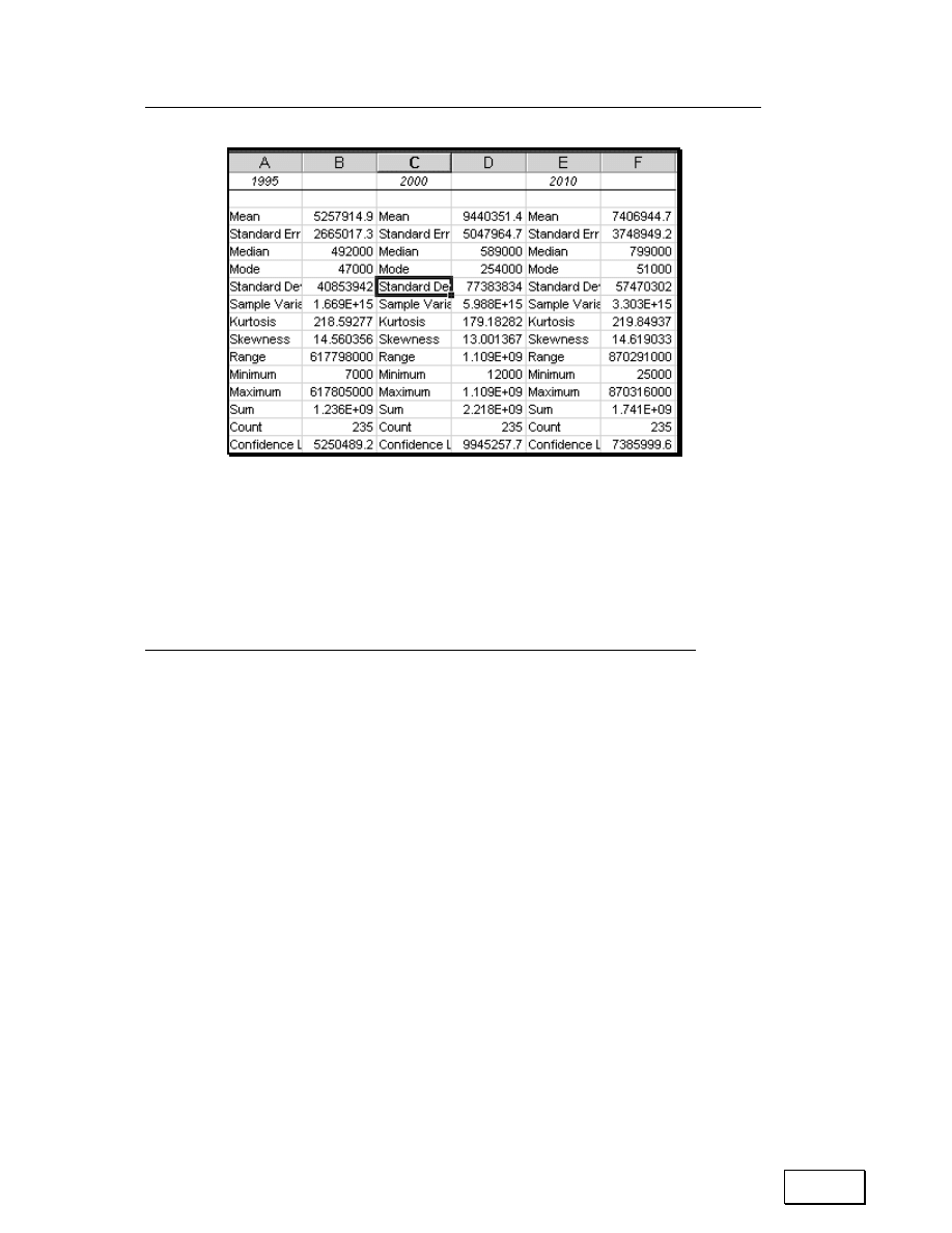
Statistical Analysis with Excel
172
Figure 146: Output of Descriptive Statistics procedure
This tool generates a report of univariate statistics for data in the input
range, providing information about the central tendency and variability of
your data
Example 2: Adding additional parameters to the descriptives table
Go to the menu option TOOLS/DATA ANALYSIS. Select the option
“
Descriptive Statistics.” In addition to the statistics requested in the
previous example, I request Excel to report on the fifth largest and fifth
smallest values for each column/series.
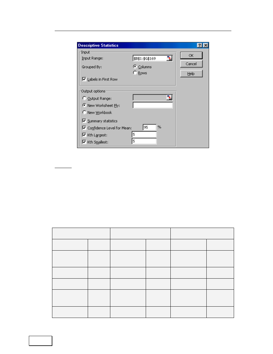
Chapter 10: Statistics Tools
173
Figure 147: The Descriptives Statistics dialog
Output
The output for the procedure is reproduced in the next table. In one
simple step, you have created a table that captures the basic statistical
attributes of several data series and the fifth highest and lowest values of
each data series.
Table 29: Output of the Descriptive Statistics tool including the Kth largest and smallest
values. The names of the three variable are: s1, s2, and x1.
s1
s2
x1
Mean
7.32
Mean
7.23
Mean
1173.00
Standard
Error
0.44
Standard
Error
0.49
Standard
Error
52.67
Median
5.31
Median
4.81
Median
1173.00
Mode
1.34
Mode
23.00
Mode
#N/A
Standard
Deviation
5.72
Standard
Deviation
6.33
Standard
Deviation
682.73
Sample
32.68
Sample
40.13
Sample
466119.22

Statistical Analysis with Excel
174
s1
s2
x1
Variance
Variance
Variance
Kurtosis
–0.22
Kurtosis
0.04
Kurtosis
–1.20
Skewness
0.95
Skewness
1.06
Skewness
0.00
Range
19.66
Range
22.00
Range
2344.00
Minimum
1.34
Minimum
1
Minimum
1
Maximum
21
Maximum
23
Maximum
2345
Sum
1229.79
Sum
1215.395
Sum
197064
Count
168
Count
168
Count
168
Largest (5)
21
Largest (5)
23
Largest (5)
2288.86
Smallest (5)
1.34
Smallest (5)
1
Smallest (5)
57.14
Confidence
Level (95.0%)
0.87
Confidence
Level (95.0%)
0.96
Confidence
Level (95.0%)
103.99
Interpretation of the statistical parameters is discussed in chapter 6, and
of Confidence levels is discussed in 7.1.
10.2
RANK AND PERCENTILE
This tool produces a table that contains the ordinal and percentage rank
of each value in a data set. You can analyze the relative standing of
values in a data set. The Percentile values can assist in learning about
the spread of the series across its range. For a series provides information
on the ranges for the lowest 25%, the next 25%, the next 25%, and the
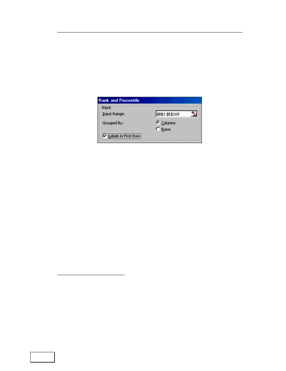
Chapter 10: Statistics Tools
175
highest 25%.
Go to
14
the menu option TOOLS/DATA ANALYSIS
15
. Select the option
“
Rank and Percentile.” The dialog is shown in the next figure.
Figure 148: Rank and Percentile tool
The result is reproduced in the next table. Each output table contains
four columns:
— The place of the data point in the data series,
— The value of the data (with the label for the series as the label
on the output column),
— The rank of the data point within the range, and
14
I do not supply the sample data for most of the examples in chapter 42 to chapter 46.
My experience is that many readers glaze over the examples and do not go through
the difficult step of drawing inferences from a result if the sample data results are
the same as those in the examples in the book.
15
If you do not see this option, then use TOOLS / ADD-INS to activate the Add-In for
data analysis. Refer to section 41.4.

Statistical Analysis with Excel
176
— The percentage rank of the data point. The columns are sorted
in order of ascending rank.
Table 30: Output of the Rank and Percentile tool
Point
s1
Rank
Percent
Point
s2
Rank
Percent
24
21.00
1
96.40%
1
23.00
1
96.40%
48
21.00
1
96.40%
25
23.00
1
96.40%
72
21.00
1
96.40%
49
23.00
1
96.40%
96
21.00
1
96.40%
73
23.00
1
96.40%
120
21.00
1
96.40%
97
23.00
1
96.40%
144
21.00
1
96.40%
121
23.00
1
96.40%
168
21.00
1
96.40%
145
23.00
1
96.40%
23
18.63
8
92.20%
2
20.07
8
92.20%
47
18.63
8
92.20%
26
20.07
8
92.20%
71
18.63
8
92.20%
50
20.07
8
92.20%
95
18.63
8
92.20%
74
20.07
8
92.20%
119
18.63
8
92.20%
98
20.07
8
92.20%
143
18.63
8
92.20%
122
20.07
8
92.20%
167
18.63
8
92.20%
146
20.07
8
92.20%
22
16.53
15
88.00%
3
17.51
15
88.00%
46
16.53
15
88.00%
27
17.51
15
88.00%
70
16.53
15
88.00%
51
17.51
15
88.00%
94
16.53
15
88.00%
75
17.51
15
88.00%
118
16.53
15
88.00%
99
17.51
15
88.00%
142
16.53
15
88.00%
123
17.51
15
88.00%
166
16.53
15
88.00%
147
17.51
15
88.00%
Interpreting the output:
The last row’s last four columns can be interpreted as—

Chapter 10: Statistics Tools
177
The 147
th
data point in the selected range has a value of 17.51,
which gives it rank 15 in the selected range, with 88% of the cells
in the range having a value less than or equal to this data point.
10.3
BIVARIATE RELATIONS— CORRELATION,
COVARIANCE
Correlation analysis
This tool and its formulas measure the relationship between two data sets
that are scaled to be independent of the unit of measurement. The
correlation coefficient depicts the basic relationship across two variables:
“
Do two variables have a tendency to increase together or to change in
opposite directions and, if so, by how much?” Bivariate correlations
measure the correlation coefficients between two variables at a time,
ignoring the effect of all other variables.
Go to the menu option TOOLS/DATA ANALYSIS
16
. Select the option
“
Correlation.”
Select the
“
Input Range” — it must have more than one data series.
16
If you do not see this option, then use TOOLS / ADD-INS to activate the Add-In for
data analysis. Refer to section 41.4.
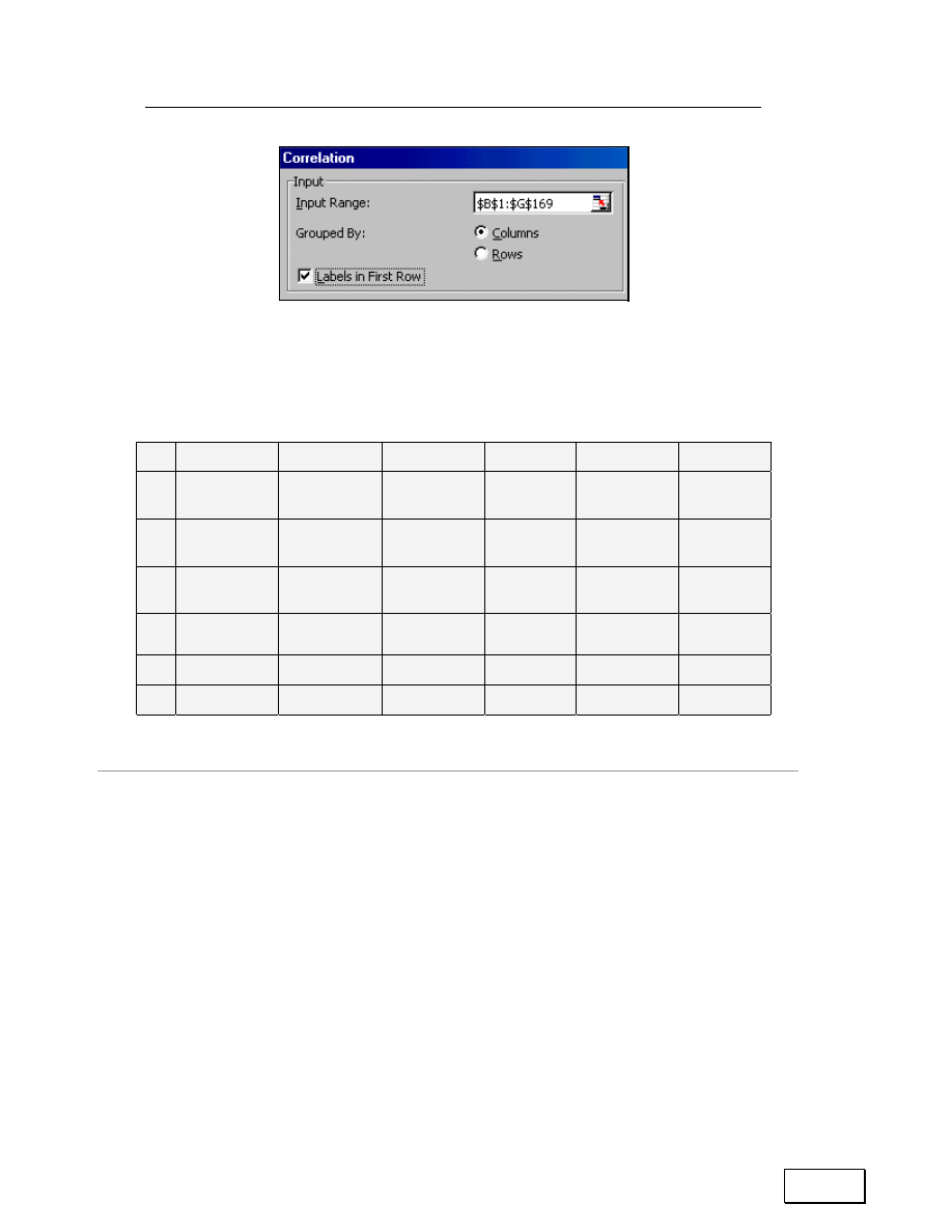
Statistical Analysis with Excel
178
Figure 149: CORRELATION
The output is reproduced in the next table.
Table 31: Output from Correlation Analysis tool
s1
s2
x1
x2
x3
x4
s1
1.00000
s2
–0.75973
1.00000
x1
–0.13434
0.13226
1.00000
x2
0.21423
0.47238
0.01658
1.00000
x3
0.20122
–0.08459
–0.15748
0.14568
1.00000
x4
–0.13567
0.12935
0.99998
0.01040
–0.15839
1.00000
Interpreting the output
— A high level of correlation is implied by a correlation coefficient
that is greater than 0.5 in absolute terms (that is, greater than
0.5 or less than –0.5).
— A mid level of correlation is implied if the absolute value of the
coefficient is greater than 0.2 but less that 0.5.
— A low level of correlation is implied if the absolute value of the
coefficient is less than 0.2.

Chapter 10: Statistics Tools
179
10.3.A
COVARIANCE TOOL AND FORMULA
The options are same as for the CORRELATION TOOL. The covariance
is dependent on the scale of measurement of the data series. Therefore,
there is no standard scale from which to infer if a covariance value is
“
high” or
“
low.” Thus, use the correlation tool that provides a uniform
scale of
“
–1 to 1.”
The coefficient of determination can be roughly interpreted as the
proportion of variance in a series that can be explained by the values of
the other series. The coefficient is calculated by squaring the correlation
coefficient.

Statistical Analysis with Excel
180

Page for Notes

Statistical Analysis with Excel
182
CHAPTER 11
HYPOTHESIS TESTING
This chapter teaches:
— Z-TESTING FOR POPULATION MEANS WHEN POPULATION
VARIANCES ARE KNOWN
— PAIRED SAMPLE T-TESTS
— T-TESTING MEANS WHEN THE TWO SAMPLES ARE FROM
DISTINCT GROUPS
— THE PRETEST— F-TESTING FOR EQUALITY IN VARIANCES
— T-TEST: TWO–SAMPLE ASSUMING UNEQUAL VARIANCES
— T-TEST: TWO–SAMPLE ASSUMING EQUAL VARIANCES
— ANOVA
The statistics Add-In provides some procedures for hypothesis testing.
The
“
Inverse Functions” in Excel
(
see 7.1) and
other statistics software can be used to build Confidence Interval’s that
provide the values for the
“
Critical Regions” for conducting hypothesis
tests. The use of the functions opens up a much wider range of possible
hypothesis tests limited only by the Inverse functions available in Excel.
I include a set of
“
testing rules” in several of the examples. These rules
will blow your mind — it will make hypothesis testing a readily
comprehensible step–by–step process. The rules will assist you in all
hypothesis tests— in Excel or otherwise.

Chapter 11: Hypothesis Testing
183
This chapter requires the Analysis ToolPak Add-Ins; chapter 9
shows how to learn how to launch the Add-Ins.
11.1
Z-TESTING FOR POPULATION MEANS WHEN
POPULATION VARIANCES ARE KNOWN
This tool performs a two–sample Z-test for means with known variances.
This tool is used to test hypotheses about the difference between two
population means.
Possible hypothesis for testing
u1 is the mean of sample one. u2 is the mean for sample two. The critical
regions are based on a 5% significance level (or, equivalently, a 95%
Confidence Interval)
(a) Two–tailed
The hypothesis
— H
0
(Null Hypothesis): u1— u2 = 1
— Ha (Alternate hypothesis): u1— u2 <> 1
Critical region:
—
“
Fail to accept” the null hypothesis if the absolute value of the
calculated Z is higher than 1.96. Examples of such Z values are:
“
+2.12” and
“
–2.12.”

Statistical Analysis with Excel
184
—
“
Fail to reject” the null hypothesis if the absolute value of the
calculated Z is lower than 1.96. Examples of such Z values are:
“
+1.78,”
“
0.00” and
“
–1.78.”
In short, if the absolute value of the Z is higher than 1.96, then one may
conclude (with 95% Confidence) that the means of the samples differ by
the hypothesized difference.
(b) One–tailed (left-tail)
The hypothesis:
— H
0
(Null Hypothesis): u1— u2 >= 1
— Ha (Alternate hypothesis): u1— u2 < 1 (one–tailed)
Critical region:
—
“
Fail to accept” the null hypothesis if the value of the calculated
Z is lower than
“
–1.64.” Examples of such Z values are:
“
–2.12”
and
“
–1.78.”
—
“
Fail to reject” the null hypothesis if left-tail)
The value of the calculated Z is greater than
“
–1.64.” Examples of such Z
values are:
“
+1.78” and
“
0.00.”
In short, if the Z is lower than
“
–1.64,” then one may conclude (with 95%
Confidence) that the means of the samples differ by the hypothesized
difference.

Chapter 11: Hypothesis Testing
185
(c) One–tailed (right-tail)
The hypothesis:
— H
0
(Null Hypothesis): u1— u2 <= 1
— Ha (Alternate hypothesis): u1— u2 > 1 (one–tailed)
Critical region:
—
“
Fail to accept” the null hypothesis if the value of the calculated
Z is greater than
“
+1.64.” Examples of such Z values are:
“
+2.12”
and
“
+1.78.”
—
“
Fail to reject” the null hypothesis if the absolute value of the
calculated Z is less than
“
+1.64.” Examples of such Z values are:
“
–1.78” and
“
0.00.”
In short, if the Z is greater than
“
+1.64,” then one may conclude (with 95%
Confidence) that the means of the samples differ by the hypothesized
difference.
Excel calculates the P or Significance value for each test you run.
— If P is less than 0.10, then the test is significant at 90%
Confidence (equivalently, the hypothesis that the means are
equal can be rejected at the 90% level of Confidence). This
criterion is considered too
“
loose” by some.

Statistical Analysis with Excel
186
— If P is less than 0.05, then the test is significant at 95%
Confidence (equivalently, the hypothesis that the means are
equal can be rejected at the 95% level of Confidence). This is the
standard criterion used.
— If P is less than 0.01, then the test is significant at 99%
Confidence (equivalently, the hypothesis that the means are
equal can be rejected at the 99% level of Confidence). This is the
strictest criterion used.
You should memorize these criteria, as nothing is more helpful in
interpreting the output from hypothesis tests (including all the tests
intrinsic to every regression, ANOVA and other analysis).
Go to TOOLS/DATA ANALYSIS
17
. Select the option
“
Z-test.” The dialog
(user-input form) that opens is shown in the next figure.
Enter the hypothesized mean difference (that is, the Null Hypothesis) into
the text-box
“
Hypothesized Mean Difference.” Enter the variances for the
two populations.
17
If you do not see this option, then use TOOLS / ADD-INS to activate the Add-In for
data analysis. Refer to section 41.4.
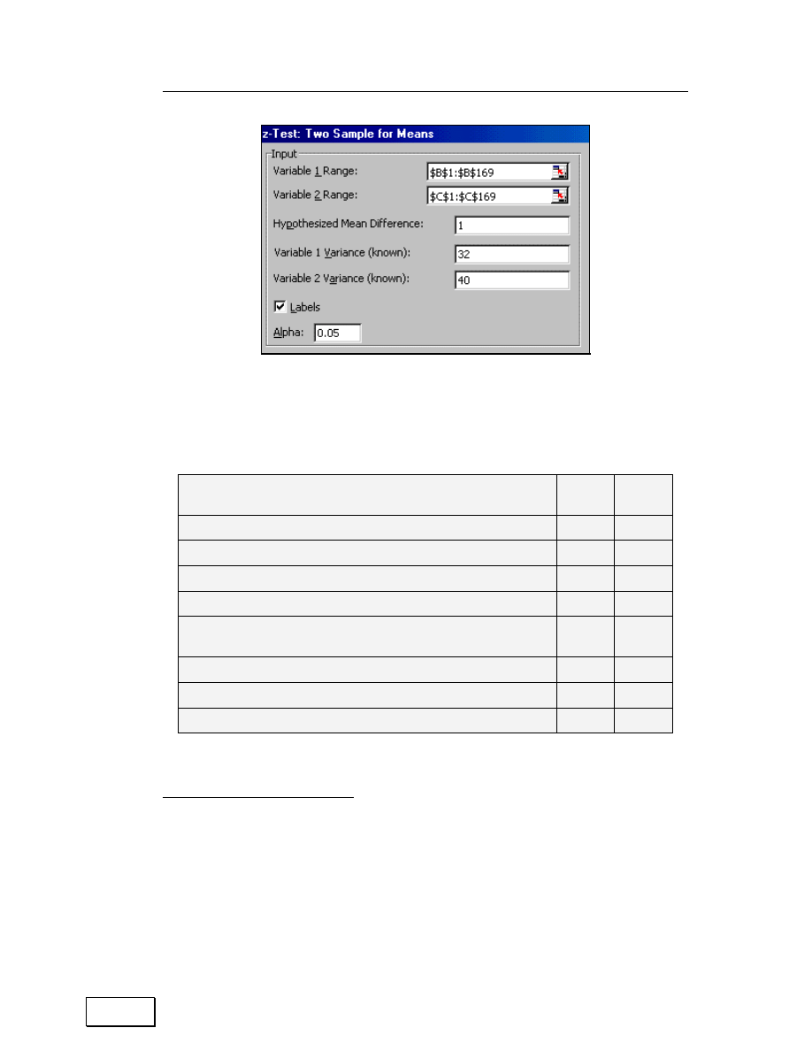
Chapter 11: Hypothesis Testing
187
Figure 150: Z-test for mean differences when population variance is known
The next table shows the result of a Z-test
18
.
Table 32: Output for Z-test for mean differences when population variance is known
Z-test: Two Sample for Means
s1
19
s2
Mean
7.3202 7.2345
Known Variance
32
40
Observations
168
168
Hypothesized Mean Difference
1.0
–1.397
P (Z< = z) one–tail
0.081
Z Critical one–tail
1.645
18
I do not supply the sample data for most of the examples in chapter 42 to chapter 46.
My experience is that many readers glaze over the examples and do not go through
the difficult step of drawing inferences from a result if the sample data results are
the same as those in the examples in the book.
19
s1 and s2 are the labels, picked up from the first row in the range b1:b25 and c1:c25.

Statistical Analysis with Excel
188
Z-test: Two Sample for Means
P (Z< = z) two–tail
0.163
Z Critical two–tail
1.960
Interpreting the output
The P value (that is
“
P (Z<= or >= z) two–tail”) of 0.081 implies that we
fail to reject the null for the two one–tail hypothesis. Moreover, Z= –1.397
implies that we
“
fail to reject” the null hypothesis because the Z is in the
acceptance region (
“
1.96,”
“
–1.96”) for the two–tail hypothesis.
The P value (that is
“
P (Z<>z) two–tail”) of 0.163 implies that we fail to
reject the null for the two–tail hypothesis. In addition, if we use a one–
tailed (left tail) test, we again fail to reject the null hypothesis because the
Z is in the acceptance region (
“
> –1.645”) for the left–tail hypothesis. If
we use a one–tail (right tail) test, we fail to reject the Null because the Z
is in the acceptance region (
“
< +1.645”) for the right–tail hypothesis.
11.2
T-TESTING MEANS WHEN THE TWO SAMPLES ARE
FROM DISTINCT GROUPS
11.2.A
THE PRETEST— F-TESTING FOR EQUALITY IN VARIANCES
The T-test is used most often to test for differences in means across
samples from distinct groups. The respondents in the two samples differ.
An example is a pair of samples from two surveys on earnings, one survey
in country A and the other in country B. The formula used in estimating
the T statistic depends on the equality of variance for the data series
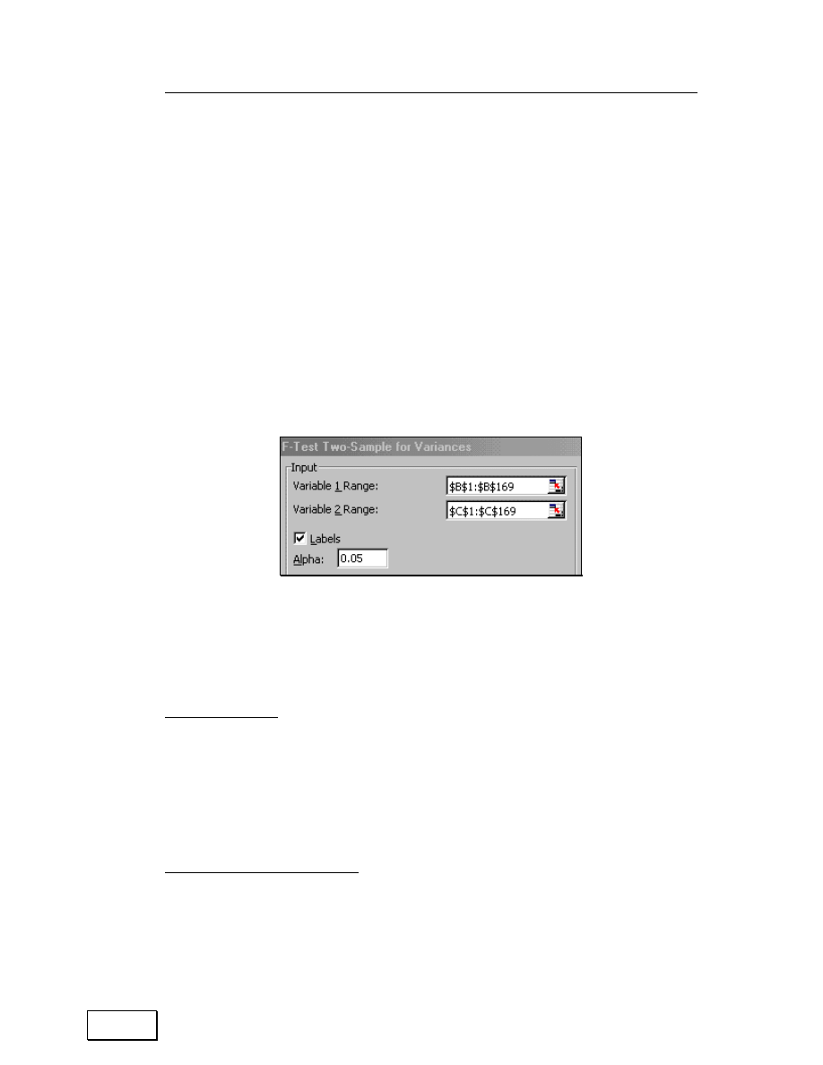
Chapter 11: Hypothesis Testing
189
across the two samples. In particular, if the variances of the two samples
are unequal the formula takes into account this difference across the
samples. An F-test is used to test for unequal variances.
The
“
F-test Two–sample for Variances” performs a test to compare the
variances across two groups of data. Launch the procedure by accessing
the menu option TOOLS/DATA ANALYSIS
20
and selecting the
“
F-test
Two–sample for Variances.”
The relevant dialog is reproduced in the next figure.
Figure 151: F-test Two–Sample for Variances
Choose the
“
alpha” for level of significance. A 0.05 level sets up a 95%
confidence test.
The hypothesis:
— H
0
(Null Hypothesis): σ
1
2
— σ
2
2
= 0
20
If you do not see this option, then use TOOLS / ADD-INS to activate the Add-In for
data analysis. Refer to section 41.4.

Statistical Analysis with Excel
190
— H
a
(Alternate hypothesis): σ
1
2
— σ
2
2
<> 0, Where σ
1
2
is the variance of
sample one, and σ
2
2
is the variance for sample two.
The F has a one–tail test only.
The next table shows the output of a typical F-test
21
.
Table 33: Output for F-test tool for equality of variances
s1
s2
Mean
7.3202
7.2345
Variance
32.6754 40.1309
Observations
168
168
Df
167
167
0.8142
P (F< = f) one–tail
0.0926
F Critical one–tail
0.8747
Interpreting the output
— The row
“
Variance” shows the estimated variance parameters.
— Inferences from the P value of
“
0.0926”:
21
I do not supply the sample data for most of the examples in chapter 42 to chapter 46.
My experience is that many readers glaze over the examples and do not go through
the difficult step of drawing inferences from a result if the sample data results are
the same as those in the examples in the book.

Chapter 11: Hypothesis Testing
191
— If P is less than 0.10, then the test is significant at 90%
Confidence (equivalently, the hypothesis that the variances are
equal can be rejected at the 90% level of Confidence). The P of
0.0926 implies the test is significant at the 90% Confidence level.
Being
“
significant” implies that the estimated F statistic lies in
the critical region and the
“
null hypothesis cannot be accepted.”
You are in the area represented by the alternate hypothesis —
the variances are unequal.
— If P is less than 0.05, then the test is significant at 95%
Confidence (equivalently, the hypothesis that the variances are
equal can be rejected at the 95% level of Confidence). The
hypothesis cannot be rejected at the 0.05 level of significance.
— If P is less than 0.01, then the test is significant at 99%
Confidence (equivalently, the hypothesis that the variances are
equal can be rejected at the 99% level of Confidence). The
hypothesis of equal variances cannot be rejected at the 0.01 level
of significance.
The test is significant only at the 0.10 level of significance. The critical
estimated F of 0.81 is higher than the critical F of 0.8747 implying that
the
“
null hypothesis of equal variances” cannot be accepted at a 0.05 level
of Confidence.
Once you know if the null hypothesis of equal variances can be accepted,
you can resolve whether to use the
“
Two–Sample T-test Assuming Equal
Variances” or
“
Two–Sample T-test Assuming Unequal Variances.”

Statistical Analysis with Excel
192
11.2.B
T-TEST: TWO–SAMPLE ASSUMING UNEQUAL VARIANCES
This T-test form assumes that the variances of both ranges of data are
unequal. Use this test when the groups under study are distinct. Use a
paired test (discussed in the next section) when there is one group before
and after a treatment.
Possible hypothesis for testing
u1 is the mean of sample one. u2 is the mean for sample two. The critical
regions are based on a 5% significance level (or, equivalently, a 95%
Confidence Interval)
(a) Two–tailed
The hypothesis
—
H
0
(Null Hypothesis): u1— u2 = 0 (or any non–zero value)
— Ha (Alternate hypothesis): u1— u2 <> 0
Critical region:
—
“
Fail to accept” the null hypothesis if the absolute value of the
calculated T is higher than 1.96. Examples of such Z values are:
“
+2.12” and
“
–2.12.”
—
“
Fail to reject” the null hypothesis if the absolute value of the
calculated T is lower than 1.96. Examples of such T values are:
“
+1.78,”
“
0.00” and
“
–1.78.”
In short, if the absolute value of the T is higher than 1.96, then one may
conclude (with 95% Confidence) that the means of the samples differ by
the hypothesized difference.

Chapter 11: Hypothesis Testing
193
(b) One–tailed (left-tail)
The hypothesis:
— H
0
(Null Hypothesis): u1— u2 >= 0
— Ha (Alternate hypothesis): u1— u2 < 0 (one–tailed)
Critical region:
—
“
Fail to accept” the null hypothesis if the value of the calculated
T is lower than
“
–1.64.” Examples of such T values are:
“
–2.12”
and
“
–1.78.”
—
“
Fail to reject” the null hypothesis if the absolute value of the
calculated T is greater than
“
–1.64.” Examples of such T values
are:
“
+1.78” and
“
0.00.”
In short, if the T is lower than
“
–1.64,” one may conclude (with 95%
Confidence) that the means of the samples differ by the hypothesized
difference.
(c) One–tailed (right-tail)
The hypothesis:
— H
0
(Null Hypothesis): u1— u2 <= 0
— Ha (Alternate hypothesis): u1— u2 > 0 (one–tailed)

Statistical Analysis with Excel
194
Critical region:
—
“
Fail to accept” the null hypothesis if the value of the calculated
T is greater than
“
+1.64.” Examples of such T values are:
“
+2.12”
and
“
+1.78.”
—
“
Fail to reject” the null hypothesis if the absolute value of the
calculated T is less than
“
+1.64.” Examples of such T values are:
“
–1.78” and
“
0.00.”
In short, if the T is greater than
“
+1.64,” then one may conclude (with 95%
Confidence) that the means of the samples differ by the hypothesized
difference.
Go to the menu option TOOLS/DATA ANALYSIS
22
. Select the option
“
T-
test: Two–Sample Assuming Unequal Variances.” The next table shows a
sample output
23
for a T-test assuming unequal variances.
Table 34: Output of Two Sample T-test (assuming unequal variances)
s1
s2
22
If you do not see this option, then use TOOLS / ADD-INS to activate the Add-In for
data analysis. Refer to section 41.4.
23
I do not supply the sample data for most of the examples in chapter 42 to chapter 46.
My experience is that many readers glaze over the examples and do not go through
the difficult step of drawing inferences from a result if the sample data results are
the same as those in the examples in the book.

Chapter 11: Hypothesis Testing
195
s1
s2
Mean
7.32
7.23
Variance
32.68
40.13
Observations
168
168
Hypothesized Mean Difference
5
Df
331
T Stat
–7.465
P (T< = t) one–tail
3.72E–13
T Critical one–tail
1.649
P (T< = t) two–tail
7.43E–13
T Critical two tail
.967
Interpreting the output
The row
“
Mean” shows the estimated means for the two samples s1 and
s2. The next column
“
Variance” displays the calculated variance for these
sample mean values.
“
Df” shows the
“
Degree of Freedom.” The degrees of
freedom equal the total sample points (the sum of the sample sizes of the
two samples) minus the one degree of freedom to account for the one
equation (the
“
hypothesized mean difference” which here is
“
u1 — u2 = 5”)
. So, degrees of freedom equals
“
168 + 168 -1 = 331”.
(a) Two–tailed
The hypothesis was:
—
H
0
(Null Hypothesis): u1— u2 = 5
— Ha (Alternate hypothesis): u1— u2 <> 5, where u1 is the mean
of sample s1 and u2 the mean of sample s2.

Statistical Analysis with Excel
196
The calculated T statistic is
“
–7.465.” The P value for the two–tailed test
is
“
3.72 multiplied by the 13th point after the decimal” or
“
0.000000000000372.” As the P value is less than 0.01, the hypothesis is
“
significant
24
“
at the 99% Confidence level or
“
alpha = 0.01” level of
significance. (The natural extension of this inference is that the
hypothesis is significant at the 95% and 90% Confidence levels also.)
The region for the two–tailed test is
“
> 1.967 or < –1.967.” In this
example, the test is significant (at a 0.05 level of significance because the
estimated T lies in the critical region. (The estimated T of
“
–7.465” lies in
the region
“
< –1.967”.)
(b) One–tailed (left-tail)
The hypothesis was:
— H
0
(Null Hypothesis): u1— u2 >= 5
— Ha (Alternate hypothesis): u1— u2 < 5, where u1 is the mean of
sample s1 and u2 the mean of sample s2.
The P value for the one–tailed test is
“
7.45 multiplied by the 13
th
point
after the decimal” or
“
0.000000000000745.” The relevant test here is the
left–tail because the T statistic is a negative value. As the P value is less
24
If a test is “significant” the implication is a “failure to accept” the null hypothesis.
The test T statistic lies in the critical region. In informal terms, the alternate
hypothesis is “correct.”

Chapter 11: Hypothesis Testing
197
than 0.01, the hypothesis is
“
significant” at the 99% Confidence level or
“
alpha = 0.01” level of significance. (The natural extension of this
inference is that the hypothesis is significant at the 95% and 90%
Confidence levels also.)
Another way to test the hypothesis is to compare the estimated T statistic
to the critical region shown in the column
“
T Critical one–tail.” The
region for the left–tailed test is
“
< –1.649”. In this example, the test is
“
significant
25
“
at a .05 level of significance because the estimated T lies in
the critical region. (The estimated T of
“
–7.465” lies in the region
“
< –
1.649”.)
(c) One–tailed (right-tail)
The hypothesis was:
— H
0
(Null Hypothesis): u1— u2 <= 5
— Ha (Alternate hypothesis): u1— u2 > 5, where u1 is the mean of
sample s1 and u2 the mean of sample s2.
The region for the right–tailed test is
“
> 1.649”. In this example, the test
is not significant because the estimated T does not lie in the critical
region. (The estimated T of
“
–7.465” is not in the region
“
>1.649”.)
25
If a test is “significant” the implication is a “failure to accept” the null hypothesis.
The test T statistic lies in the critical region. In informal terms, the alternate
hypothesis is “correct.”

Statistical Analysis with Excel
198
11.2.C
T-TEST: TWO–SAMPLE ASSUMING EQUAL VARIANCES
This tool performs a two–sample student's T-test— under the assumption
that the variances of both data sets are equal. The hypothesis and
interpretation of results is the same as for the Two–Sample Assuming
Unequal Variances. (See previous sub-section).
The next table shows the result this type of test
26
.
11.3
PAIRED SAMPLE T-TESTS
This tool performs a paired two–sample T-test to deduce whether the
difference between the sample means is statistically distinct from a
hypothesized difference. This T-test form does not assume that the
variances of both populations are equal. You can use a paired test when
there is a natural pairing of observations in the samples, such as when a
sample group is tested twice— before and after an experiment. The tested
groups form a
“
Paired Sample” with the same respondents sampled
“
before” and
“
after” an event.
Go to the menu option TOOLS/DATA ANALYSIS
27
. Select the option
“
T-
26
I do not supply the sample data for most of the examples in chapter 42 to chapter 46.
My experience is that many readers glaze over the examples and do not go through
the difficult step of drawing inferences from a result if the sample data results are
the same as those in the examples in the book.
27
If you do not see this option, then use TOOLS / ADD-INS to activate the Add-In for
data analysis. Refer to section 41.4.
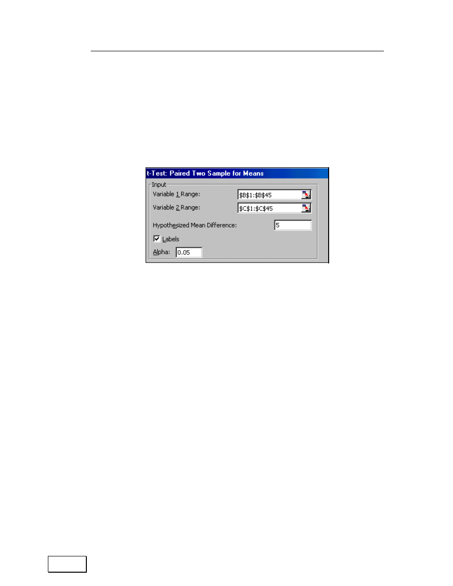
Chapter 11: Hypothesis Testing
199
test: Two–Sample Assuming Unequal Variances.” The relevant dialog is
shown in the next figure.
The range must consist of a single column or row and contain the same
number of data points as the first range.
Figure 152: T-test for Paired Samples
Place the hypothesized difference in means into the checkbox
“
Hypothesized Mean Difference.” In this example, one is using the
hypothesis:
“
H
0
(Null Hypothesis): mean difference > 5”. See the next figure for
an example of setting the hypothesis for testing. Set a
hypothesized mean difference of zero to test the standard
hypothesis that the
“
Means for the two groups/samples are
statistically different.”
The level of significance for the hypothesis tests should be placed in
the checkbox
“
Alpha.” If you desire a significance level of
“
alpha =
.05” (that is, a Confidence level of 95%), then write in
“
.05” into the
checkbox Alpha. The next figure illustrates this.

Statistical Analysis with Excel
200
Possible hypothesis for testing
u1 is the mean of sample one. u2 is the mean for sample two. The critical
regions are based on a 5% significance level (or, equivalently, a 95%
Confidence Interval)
(a) Two–tailed
The hypothesis
—
H
0
(Null Hypothesis): u1— u2 = 0
— Ha (Alternate hypothesis): u1— u2 <> 0
Critical region:
—
“
Fail to accept” the null hypothesis if the absolute value of the
calculated T is higher than 1.96. Examples of such T values are:
“
+2.12” and
“
–2.12.”
—
“
Fail to reject” the null hypothesis if the absolute value of the
calculated T is lower than 1.96. Examples of such T values are:
“
+1.78,”
“
0.00” and
“
–1.78.”
In short, if the absolute value of the T is higher than 1.96, then one may
conclude (with 95% Confidence) that the means of the samples differ by
the hypothesized difference.
(b) One–tailed (left-tail)
The hypothesis:
— H
0
(Null Hypothesis): u1— u2 >= 0

Chapter 11: Hypothesis Testing
201
— Ha (Alternate hypothesis): u1— u2 < 0 (one–tailed)
Critical region:
—
“
Fail to accept” the null hypothesis if the value of the calculated
T is lower than
“
–1.64.” Examples of such T values are:
“
–2.12”
and
“
–1.78.”
—
“
Fail to reject” the null hypothesis if the absolute value of the
calculated T is greater than
“
–1.64”. Examples of such T values
are:
“
+1.78” and
“
0.00.”
In short, if the T is lower than
“
–1.64,” then one may conclude (with 95%
Confidence) that the means of the samples differ by the hypothesized
difference.
(c) One–tailed (right-tail)
The hypothesis:
— H
0
(Null Hypothesis): u1— u2 <= 1
— Ha (Alternate hypothesis): u1— u2 > 1 (one–tailed)
Critical region:
—
“
Fail to accept” the null hypothesis if the value of the calculated
T is greater than
“
+1.64.” Examples of such T values are:
“
+2.12”
and
“
+1.78.”
—
“
Fail to reject” the null hypothesis if the absolute value of the
calculated T is less than
“
+1.64.” Examples of such T values are:
“
–1.78” and
“
0.00.”

Statistical Analysis with Excel
202
In short, if the T is greater than
“
+1.64,” then one may conclude (with 95%
Confidence) that the means of the samples differ by the hypothesized
difference.
Excel calculates the P or Significance value for each test you run.
— If P is less than 0.10, then the test is significant at 90%
Confidence (equivalently, the hypothesis that the means are
equal can be rejected at the 90% level of Confidence). This
criterion is considered too
“
loose” by some.
— If P is less than 0.05, then the test is significant at 95%
Confidence (equivalently, the hypothesis that the means are
equal can be rejected at the 95% level of Confidence). This is the
standard criterion used.
— If P is less than 0.01, then the test is significant at 99%
Confidence (equivalently, the hypothesis that the means are
equal can be rejected at the 99% level of Confidence). This is the
strictest criterion used.
You should memorize these criteria, as nothing is more helpful in
interpreting the output from hypothesis tests (including all the tests
intrinsic to every regression, ANOVA and other analysis). The output for

Chapter 11: Hypothesis Testing
203
such a test is shown in the next table
28
.
Table 35: Output from a T-test for Paired Samples. The text in italics has been inserted by
the author.
First
sampling
Second
sampling
Mean
152
145
Variance
126
114
Observations
44
44
Pearson Correlation
0.999693
Hypothesized Mean Difference
5
Df
43
T Stat
26.76
26.76 is the T
estimated from the
data
One–tailed test
P (T< = t) one–tail
0.00
T Critical one–tail
1.68
1.68 is the
“
T cut–off
Critical Value” from
T-Tables
Two–tailed Test
P (T< = t) two–tail
0.00
T Critical two–tail
2.02
2.02 is the
“
T cut–off
Critical Value” from
T-Tables
Interpretation:
One–tailed test
P (T< = t) one–tail
0.00
Thus, significant at 99%
28
I do not supply the sample data for most of the examples in chapter 42 to chapter 46.
My experience is that many readers glaze over the examples and do not go through
the difficult step of drawing inferences from a result if the sample data results are
the same as those in the examples in the book.

Statistical Analysis with Excel
204
One–tailed test
T Critical one–tail (positive
for positive tail test, negative
for negative tail)
1.68
—1.68
2.02 is the
“
T cut–off Critical Value” from T-
Tables for alpha = 0.05 and Df = 43
Inferential Analysis:
— Fail to reject null (1-tailed for null hypothesizing in a negative direction: H
0
(Null
Hypothesis): mean<5)
— Fail to accept null if H0 (Null Hypothesis): mean>5.
Two–tailed Test
P (T< = t) two–tail
0.00
Thus, significant at 99%
T Critical two–tail (compare
absolute value of T- stat from
the data with this absolute
value)
2.02
This is the
“
T cut–off Critical Value” from T-
Tables for alpha = 0.025 and Df = 43
Inferential Analysis:
— For two–tailed test, fail to accept null at 99% Confidence
11.4
ANOVA
This tool performs simple analysis of variance (ANOVA) to test the
hypothesis that means from two or more samples are equal (drawn from
populations with the same mean). This technique expands on the tests for
two means, such as the T-test.
Go to the menu option TOOLS/DATA ANALYSIS
29
. Select the option
“
ANOVA: Single Factor.” The input range must consist of two or more
29
If you do not see this option, then use TOOLS / ADD-INS to activate the Add-In for
data analysis. Refer to section 41.4.
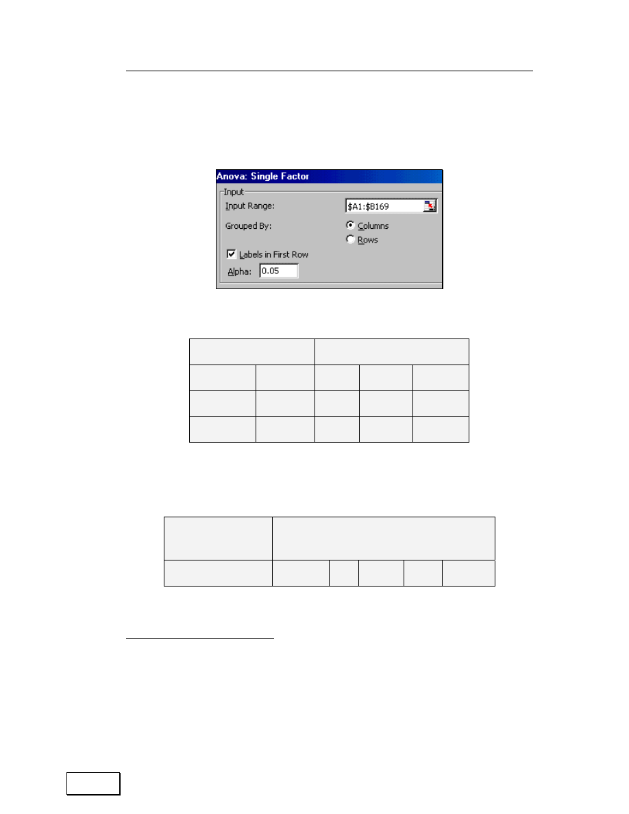
Chapter 11: Hypothesis Testing
205
adjacent ranges of data arranged in columns or rows. A sample output
30
is shown in the next few tables.
Figure 153: Single Factor ANOVA
Table 36: Output from Single Factor ANOVA — a
ANOVA: Single Factor
Groups
Count
Sum
Average Variance
s1
168
1229.8
7.3
32.7
s2
168
1215.4
7.2
40.1
The first table shows some descriptive statistics for the samples.
Table 37: Output from Single Factor ANOVA — b
ANOVA
Source of Variation
SS
Df
MS
F
P–value
30
I do not supply the sample data for most of the examples in chapter 42 to chapter 46.
My experience is that many readers glaze over the examples and do not go through
the difficult step of drawing inferences from a result if the sample data results are
the same as those in the examples in the book.

Statistical Analysis with Excel
206
ANOVA
Between Groups
0.62
1
0.62
0.017
0.90
Within Groups
12158.65 334 36.403
Total
12159.27 335
Interpreting the output
The information on
“
Between Groups” is derived from the difference in
means and variances across the groups. In an ANOVA, the number of
groups may exceed two.
— The test is analyzing the variance as measured by the SS
“
Sum of
Squares” of the
“
dependent” series. The total Sum of Squares is
12159.27. Of this, 0.62 can be explained by the differences across the
means of the two groups. The other 12158.65 is explained by the
differences across individual values of the
“
dependent” series.
• Sum of Squares = Sum of Squares for Between Groups + Sum of
Squares for Within Groups
— The MS is the
“
Mean Sum of Squares” and is estimated by dividing the
SS by the degrees of freedom. Therefore, the MS for
“
Between Groups”
equals (0.62/1) = 0.62. (Note that
“
ANOVA = Analysis of Variance.”)
The MS for
“
Within Groups” equals (12158.65/334) = 36.403. The MS
may be informally interpreted as
“
Sum of Squares Explained per Degree
of Freedom.”
•
Mean Sum of Squares = (Sum of Squares)/ (Degrees of Freedom)

Chapter 11: Hypothesis Testing
207
— The ANOVA uses an F-test to determine if
“
Between Groups”
information (the number 0.62 in the column
“
Between Groups” Source
of Variation MS) provides sufficient additional information to improve
the ability of the data to explain the variance in the
“
dependent” series.
The ANOVA is asking
“
Does the Between Groups Sum of Squares
Explained per Degree of Freedom” divided by the
“
Within Groups Sum
of Squares” provide an F that is large enough to justify the statement
“
The use of Between Groups information explains a statistically
significant amount of the Sum of Squares of the dependent series.”
• F = (Mean Sum of Squares Between Groups)/ (Mean Sum of
Squares Within Groups)
— All ANOVA tests (including the ANOVA output from a regression) can
be interpreted in the same way –
• F = [ (Increase in ability of model to explain the Sum of
Squares)/ (Degrees of Freedom) /
(Total Sum of Squares) / (Degrees of Freedom)]

Statistical Analysis with Excel
208

Page for Notes

Statistical Analysis with Excel
210
CHAPTER 12
REGRESSION
This chapter discusses the following topics:
— ASSUMPTIONS UNDERLYING REGRESSION MODELS
— CONDUCTING THE REGRESSION
This chapter requires the Analysis ToolPak Add-Ins; chapter 9
shows how to learn how to launch the Add-Ins.
12.1
ASSUMPTIONS UNDERLYING REGRESSION
MODELS
The field of econometrics uses regression analysis to create quantitative
models that can be used to predict the value of a series if one knows the
value of several other variables. For example, the wage per hour can be
predicted if one knows the values of the variables that constitute the
regression equation. This is a big leap of faith from a correlation or
Confidence interval estimate. In a correlation, the statistician is not
presuming or implying any causality or deduction of causality. On the
other hand, regression analysis is used so often (probably even abused)
because of its supposed ability to link cause and effect. Skepticism of
causal relationships is not only healthy but also important because real
power of regression lies in a comprehensive interpretation of the results.

Chapter 12: Regression
211
Regression models are used to test the statistical validity of causal
relation presumed in theory or hypothesis. Regression can never be
divorced from the hypothesis it is testing. The construction of the model
has to be based upon the hypothesis, and not on the availability of the
data. Therefore, if you believe you have a valid hypothesis, but do not
have the correct data series to represent each factor in your hypothesis,
the best practice is not running a regression analysis.
On the other hand, the method of throwing in all variables into the model
and making the computer select the best model is a misleading technique
that sadly has gained popularity because of the belief that the best model
is the one that fits the data the best.
The best models can only be a subset of
“
valid models.” (That is, models
that have passed all diagnostic test for presumptions for conforming to the
assumptions required by a regression.) Furthermore, note that if the
model is shown to
“
not fit” the data, or the expected relationship between
variables is estimated as negligible, you still have valid results. The
variance between the hypothesis and the results is always important and
can give rise to a new perspective relative to the hypothesis.
The process of interpretation is called inferential analysis and is far more
important than the actual number punching. Inferential analysis also
includes testing if the data and model have complied with the strong
assumptions underlying a regression model.
The very veracity and validity depends upon several diagnostic tests.
Unfortunately, many econometricians do not perform the diagnostic
testing or simply lie about the inferences and conclusions derived from the
model.
Our book
“
Interpreting Regression Output” provides a summary table (a

Statistical Analysis with Excel
212
cheat–sheet for you!) that lists the implications of the invalidity of
assumptions. (The book can be purchased at http://www.vjbooks.net).
This summary provides, in one page, what other books have spread out
over many chapters. Please use this table as a checklist before you
interpret any model. Most statistic professors and textbooks teach the
interpretation of regression results before discussing the issue of validity.
You will save yourself a lot of grief if you always perform diagnostics after
running a regression model.
Once you have a valid model, interpret the results in the logical sequence
shown in the table interpreting regression output in our book
“
Interpreting Regression Output.” This table will provide a framework
and flowchart for interpretation thereby enabling a structured and
comprehensive inferential analysis.
12.1.A
ASSUMPTION 1: THE RELATIONSHIP BETWEEN ANY ONE
INDEPENDENT SERIES AND THE DEPENDENT SERIES CAN BE
CAPTURED BY A STRAIGHT LINE IN A 2–AXIS GRAPH
This is also called the assumption of linearity in the regression
coefficients. (None of the regression coefficients — the betas — should
have an exponential power or any other non— linear transformation.)
12.1.B
ASSUMPTION 2: THE INDEPENDENT VARIABLES DO NOT
CHANGE IF THE SAMPLING IS REPLICATED
The independent variables are truly independent— the model assumes is
using deviations across the X variables to explain the dependent series.
The regression attempts to explain the dependent series’ variations across

Chapter 12: Regression
213
the combination of values of the independent variables.
If repeated samples are used, the model predicts the same predicted
dependent series for each combination of X values, but— across the
samples— the observed Y may differ across the same combination of X
values. (The gap between the predicted and observed Y values is the
residual or error.)
12.1.C
ASSUMPTION 3:
THE SAMPLE SIZE MUST BE GREATER
THAN THE NUMBER OF INDEPENDENT VARIABLES (N
SHOULD BE GREATER THAN K–1)
This assumption ensures that a basic mathematical postulate is adhered
to by the regression algorithm. A system of simultaneous equations is
only
“
determined
31
“
if the number of equations
32
is greater than the
number of unknowns. That is, only if the number of regression
coefficients— K minus 1, the subtraction accounting for the coefficient for
the intercept).
What information is
“
known” prior to running the regression?
— All values of the independent variables are known first. In
theory, the independent variables are the
“
experiment.”
31
That is, it can be solved to estimate the optimization parameters — the regression
coefficients in the case of a regression
32
The sample size N in the case of a regression

Statistical Analysis with Excel
214
— Once the
“
experiment” is conducted, the values of the dependent
series Y are known. (Not that this
“
experiment” analogy holds
even if the data for the independent and dependent variables are
obtained from the same data collection survey.)
— The regression minimizes the sum of the squared residuals,
which is the same as minimizing the square of the difference
between the observed and the predicted dependent series. The
number of residuals equals the number of observations. Thus,
the number of equations equals the number of observations.
What information is
“
unknown” prior to running the regression?
The regression coefficients — the betas — are unknown. Once the
regression coefficients are known, one can estimate the predicted
dependent variables, errors/residuals, R–square, etc. If X does not vary,
then the series cannot have any role in explaining the variation in Y. The
number of unknowns equals the number of regression coefficients.
12.1.D
ASSUMPTION 4: NOT ALL THE VALUES OF ANY ONE
INDEPENDENT SERIES CAN BE THE SAME
A model uses the effect of variation in X to explain variation in Y. If X
does not vary, then the series cannot have any role in explaining the
variation in Y.
Note that the formulas for estimating the regression coefficients — the
betas — use the
“
squared deviations from mean” in the denominator of
the formula. If the X values do not vary then all the values equal the
mean implying that the
“
squared deviations from mean” is zero. This will

Chapter 12: Regression
215
make the regression coefficient indeterminate because the denominator of
the formula equals zero.
12.1.E
ASSUMPTION 5:
THE RESIDUAL OR DISTURBANCE
ERROR TERMS FOLLOW SEVERAL RULES
This is the most important assumption, and most diagnostic tests are
checking for the observance of this assumption. In several textbooks, you
will find this assumption broken into parts, but I prefer to list the rules of
Assumption 5:
Assumption 5a: The mean/average or expected value of the disturbance
equals zero
If not, then you know that the model has a systemic bias, which makes it
inaccurate, especially because one does not typically know what is causing
the bias.
Assumption 5b: The disturbance terms all have the same variance
This assumption is also called homoskedasticity. Given that the expected
value of any disturbance equals zero, if one disturbance has a higher
variance than the other one, it implies that the observation underlying
this high variance should be given less importance because its relative
accuracy is suspect. (This is the reason that weighted regression is used
to correct for the nonconformity with this rule.)

Statistical Analysis with Excel
216
Assumption 5c: A disturbance term for one observation should have no
relation with the disturbance terms for other observations or with any of
the independent variables
The disturbance term must be truly random — one should not be able to
predict or guess the value of any disturbance term given any of the
information on the model data. The disturbance term is also called the
error term. This error is assumed random. If this is not the case, then
your model may have failed to capture all the underlying independent
variables, incorrectly measured independent variables, or have correlation
between successive observations in a series Sorted by one of the
independent variables.
Typically, Time Series data series suffers from the problem of disturbance
terms being related to the values of previous periods. It is for this reason
that times series analysis requires special data manipulation procedures
prior to creating any prediction model.
Assumption 5d: There is no specification bias
This is the most crucial assumption because a mistake in specifying the
equation for regression is the responsibility of the statistician. One
cannot blame the nature of the data for this problem. One type of
specification bias is the use of an incorrect functional form. For example,
you have a specification bias if you use a linear function when a
logarithmic or exponential function should be used.
The other type of specification bias is when the model does not include a
relevant data series. This is the most common type of error of oversight
by because of the incorrect habit in creating a hypothesis only after
looking at the available data. This approach may result in the exclusion
of an important series that may not be in the available data set.

Chapter 12: Regression
217
Remember that a regression is based on a hypothesis — you always define
the hypothesis first. After that, look for data that can capture all of the
variables in the hypothesis. If you do not find the data to represent an
important factor, then you should not use regression analysis. Another
bad habit is the dropping of variables from a model if the coefficient is
seen to have no impact on the dependent series. It is better to have an
irrelevant or excess series, then to drop a relevant series. In fact, the
result that a factor has no impact on the dependent series often provides
compelling insight.
Assumption 5e: The disturbance terms have a Normal Density Function
The use of the F-test for validating the model and the T-tests for
validating individual coefficients is predicated on the presumption that
the disturbance terms follow a Normal Density Function.
12.1.F
ASSUMPTION 6: THERE ARE NO STRONG LINEAR
RELATIONSHIPS AMONG THE INDEPENDENT VARIABLES
If the relationships are strong, then the regression estimation will not be
able to isolate the impact of each independent series. Related to this is
another rule: there should be no endogenity in the model. This means
that none of the independent variables should be dependent on other
variables. An independent series should not be a function of another
independent series.
Every estimate in a regression is not only a point estimate of the
parameter of the expected value of the parameter. The regression
estimates the expected value (mean) of the parameter, its variance, and
its Density Function (the assumption of normality provides the shape of

Statistical Analysis with Excel
218
the Density Function). The mean and standard error are estimated by the
model. There is a pair of such estimates for each coefficient (each BETA),
each disturbance term, and each predicted value of the dependent series.
Note: The dependent series is that whose values you are trying to predict
(or whose dependence on the independent variables is being studied). It is
also referred to as the
“
Explained” or
“
Endogenous” series, or as the
“
Regressand.”
The independent variables are used to explain the values of the dependent
series. The values of the independent variables are not being
explained/determined by the model — thus, they are
“
independent” of the
model. The independent variables are also called
“
Explanatory” or
“
Exogenous” variables. They are also referred to as
“
Regressors.”
I do not show the details of regression analysis. Please refer to
our book “Interpreting regression Output” available at
http://www.vjbooks.net.
12.2
CONDUCTING THE REGRESSION
Go to the menu option TOOLS/DATA ANALYSIS
33
. Select the option
“
Regression” as shown in Figure 154.
33
If you do not see this option, then use TOOLS / ADD-INS to activate the Add-In for
data analysis. Refer to section 41.4.
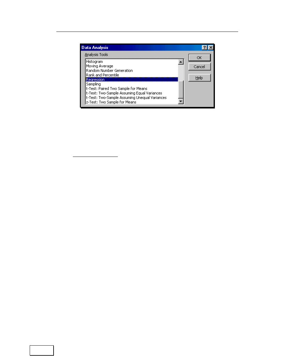
Chapter 12: Regression
219
Figure 154: Selecting the regression procedure
Choose the exact cell references for the Y and X ranges. So do not choose
“
C:D;” instead, choose C1:D235, as shown in Figure 155.
Other restrictions:
– All the X variables have to be in adjacent columns
and
– The data cannot have missing values
Choose all other options as shown in Figure 155.
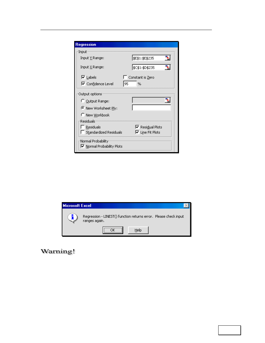
Statistical Analysis with Excel
220
Figure 155: The completed Regression dialog
There should be no missing values in the range defined. Otherwise, you
get the error message shown in Figure 156.
Figure 156: Error message if you select an incorrect range for the regression
The statistical Add-In provided with Excel has many
limitations— it does only a few procedures, has bugs, and cannot handle
complex data. (For example, it cannot do a regression if there are any
missing values.) Fortunately, some other companies have created Add-Ins
that provides comprehensive statistics capabilities. Links to such Add-Ins
can be accessed at the URL
http://www.vjbooks.net/products/publications/Excel/Excel.htm..

Chapter 12: Regression
221
I do not show the output or its detailed interpretation. Please
refer to our book
“
Interpreting regression Output” available at
http://www.vjbooks.net.
A brief summary of interpretation guidelines is presented in the next
section.
12.3
BRIEF GUIDELINE FOR INTERPRETING
REGRESSION OUTPUT
Table 38: Interpreting regression output
Name Of
Statistic/
Chart
What Does It
Measure Or
Indicate?
Critical Values
Comment
Sig.-F
Whether the model
as a whole is
significant. It
tests whether R-
square is
significantly
different from zero
– below .01 for
99% confidence in
the ability of the
model to explain
the dependent
variable
– below .05 for
95% confidence in
the ability of the
model to explain
the dependent
variable
– below 0.1 for
90% confidence in
the ability of the
model to explain
the dependent
variable
The first statistic to look
for in the output.
If Sig.-F is insignificant,
then the regression as a
whole has failed. No
more interpretation is
necessary (although some
disagree on this point).
You must conclude that
the
“
Dependent variable
cannot be explained by
the
independent/explanatory
variables.” The next
steps could be rebuilding
the model, using more
data points, etc.
RSS, ESS &
TSS
The main function
of these values lies
in calculating test
statistics like the
The ESS should
be high compared
to the TSS (the
ratio equals the R-
square). Note for
If the R-squares of two
models are very similar
or rounded off to zero or
one, then you might
prefer to use the F-test

Statistical Analysis with Excel
222
Name Of
Statistic/
Chart
What Does It
Measure Or
Indicate?
Critical Values
Comment
F-test, etc.
interpreting the
table, column
“
Sum of Squares”:
“Total” =TSS,
“Regression” =
ESS, and
“Residual” = RSS
formula that uses RSS
and ESS.
SE of
Regression
The standard error
of the estimate
predicted
dependent variable
There is no critical
value. Just
compare the std.
error to the mean
of the predicted
dependent
variable. The
former should be
small (<10%)
compared to the
latter.
You may wish to
comment on the SE,
especially if it is too large
or small relative to the
mean of the
predicted/estimated
values of the dependent
variable.
-Square
Proportion of
variation in the
dependent variable
that can be
explained by the
independent
variables
Between 0 and 1.
A higher value is
better.
This often mis-used
value should serve only
as a summary measure of
Goodness of Fit. Do not
use it blindly as a
criterion for model
selection.
Adjusted R-
square
Proportion of
variance in the
dependent variable
that can be
explained by the
independent
variables or R-
square adjusted
for # of
independent
variables
Below 1. A higher
value is better
Another summary
measure of Goodness of
Fit. Superior to R-square
because it is sensitive to
the addition of irrelevant
variables.
-Ratios
The reliability of
our estimate of the
individual beta
Look at the p-
value (in the
column
“
Sig.”) it
must be low:
- below .01 for
99% confidence in
For a one-tailed test (at
95% confidence level), the
critical value is
(approximately) 1.65 for
testing if the coefficient is
greater than zero and
(approximately) -1.65 for

Chapter 12: Regression
223
Name Of
Statistic/
Chart
What Does It
Measure Or
Indicate?
Critical Values
Comment
the value of the
estimated
coefficient
- below .05 for
95% confidence in
the value of the
estimated
coefficient
- below .1 for 90%
confidence in the
value of the
estimated
coefficient
testing if it is below zero.
Confidence
Interval for
beta
The 95%
confidence band
for each beta
estimate
The upper and
lower values give
the 95%
confidence limits
for the coefficient
Any value within the
confidence interval
cannot be rejected (as the
true value) at 95% degree
of confidence
Charts:
Scatter of
predicted
dependent
variable and
residual
(Preferably
after
standardizing
the series)
Make a
scatter chart
manually
after running
the regression
in Excel. **
Mis-specification
and/or
heteroskedasticity
There should be
no discernible
pattern. If there
is a discernible
pattern, then do
the RESET and/or
DW test for mis-
specification or
the White’s test
for
heteroskedasticity
Extremely useful for
checking for breakdowns
of the classical
assumptions, i.e. - for
problems like mis-
specification and/or
heteroskedasticity. At
the top of this table, we
mentioned that the F-
statistic is the first
output to interpret.
Some may argue that the
PRED-RESID plot is
more important.
Charts: plots
of residuals
against
independent
variables.
(Preferably
after
standardizing
Heteroskedasticity
There should be
no discernible
pattern. If there
is a discernible
pattern, then
perform a formal
test.
Common in cross-
sectional data.
If a partial plot has a
pattern, then that
variable is a likely
candidate for the cause of

Statistical Analysis with Excel
224
Name Of
Statistic/
Chart
What Does It
Measure Or
Indicate?
Critical Values
Comment
the series)
Make a
scatter chart
manually
after running
regression**
heteroskedasticity.
Charts:
Histograms of
residuals. No
need to
standardize.
Make an area
chart after
running the
regression in
Excel**
Provides an idea
about the
distribution of the
residuals
The distribution
should look like a
normal
distribution
A good way to observe the
actual behavior of our
residuals and to observe
any severe problem in the
residuals (which would
indicate a breakdown of
the classical
assumptions)
** (a) Estimate the series
“
predicted” by using the regression formula:
Predicted_Y= constant + B
1
X
1
+… + B
k
X
k
.
(b) Standardize the series of predicted values using the function
INSERT/ FUNCTION/ STATISTICAL/ STANDARDIZE.
(c) Estimate the residual, by using the formula:
Residual= Y — Predicted_Y
(d) Standardize the series of residuals using the function INSERT/
FUNCTION/ STATISTICAL/ STANDARDIZE
(e) make the charts using the standardized series. See book two in
this series — Charting in Excel — for more on making charts.

Chapter 12: Regression
225
12.4
BREAKDOWN OF CLASSICAL ASSUMPTIONS:
VALIDATION AND CORRECTION
Basic validation can be conducted using procedures mentioned in the
previous table. Excel does not have procedures for more advanced testing.
The corrective procedures are not available in Excel.
The validation and corrective procedures are available in Add-Ins for
statistics. Links to such Add-Ins can be accessed at the URL
http://www.vjbooks.net/products/publications/Excel/Excel.htm.
For more on this topic, please refer to our book
“
Interpreting
regression Output” available at http://www.vjbooks.net.

Statistical Analysis with Excel
226

Page for Notes

Statistical Analysis with Excel
228
CHAPTER 13
OTHER TOOLS FOR STATISTICS
This chapter briefly touches on the following topics:
— SAMPLING ANALYSIS
— RANDOM NUMBER GENERATION
— TIME SERIES
— EXPONENTIAL SMOOTHING, MOVING AVERAGE ANALYSIS
This chapter requires the Analysis ToolPak Add-Ins; chapter 9
shows how to learn how to launch the Add-Ins.
13.1
SAMPLING ANALYSIS
This tool creates a sample from a population by treating the input range
as a population. You can use a representative sample when the
population is too large to process or chart. You can also create a sample
that contains only values fro a particular part of a cycle if you believe that
the input data is periodic Excel draws samples from the first column, then
the second column, and so on.
Access the feature through the menu path TOOLS/DATA ANALYSIS and
choose the procedure
“
Sampling.”
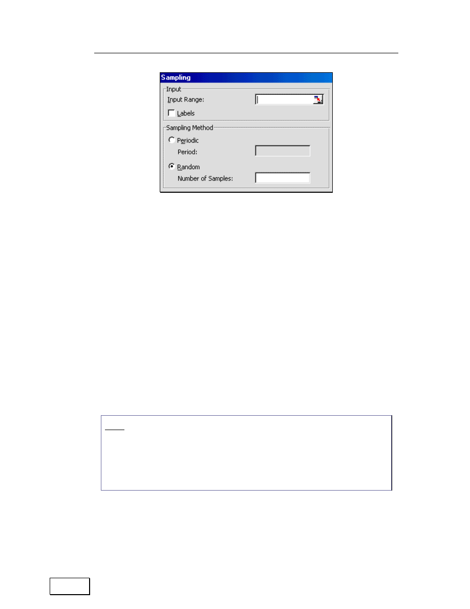
Chapter 13: Other Tools for Statistics
229
Figure 157: Sampling
Sampling Method: choose Periodic or Random to indicate the sampling
interval you want.
Period: Enter the periodic interval at which you want sampling to take
place. The interval value in the input range and every period’s value
thereafter are copied to the output column.
Random & Number of Samples: Number of random values you desire in
the output column. Excel draws each value from a random position in the
input range. (Consequently, a value may be drawn more than once.)
Output Range: Data is written in a single column below the cell.
Note:
If you selected Periodic, the number of values in the output table is
equal to the number of values in the input range, divided by the
sampling rate. If you selected Random, the number of values in the
output table is equal to the number of samples.
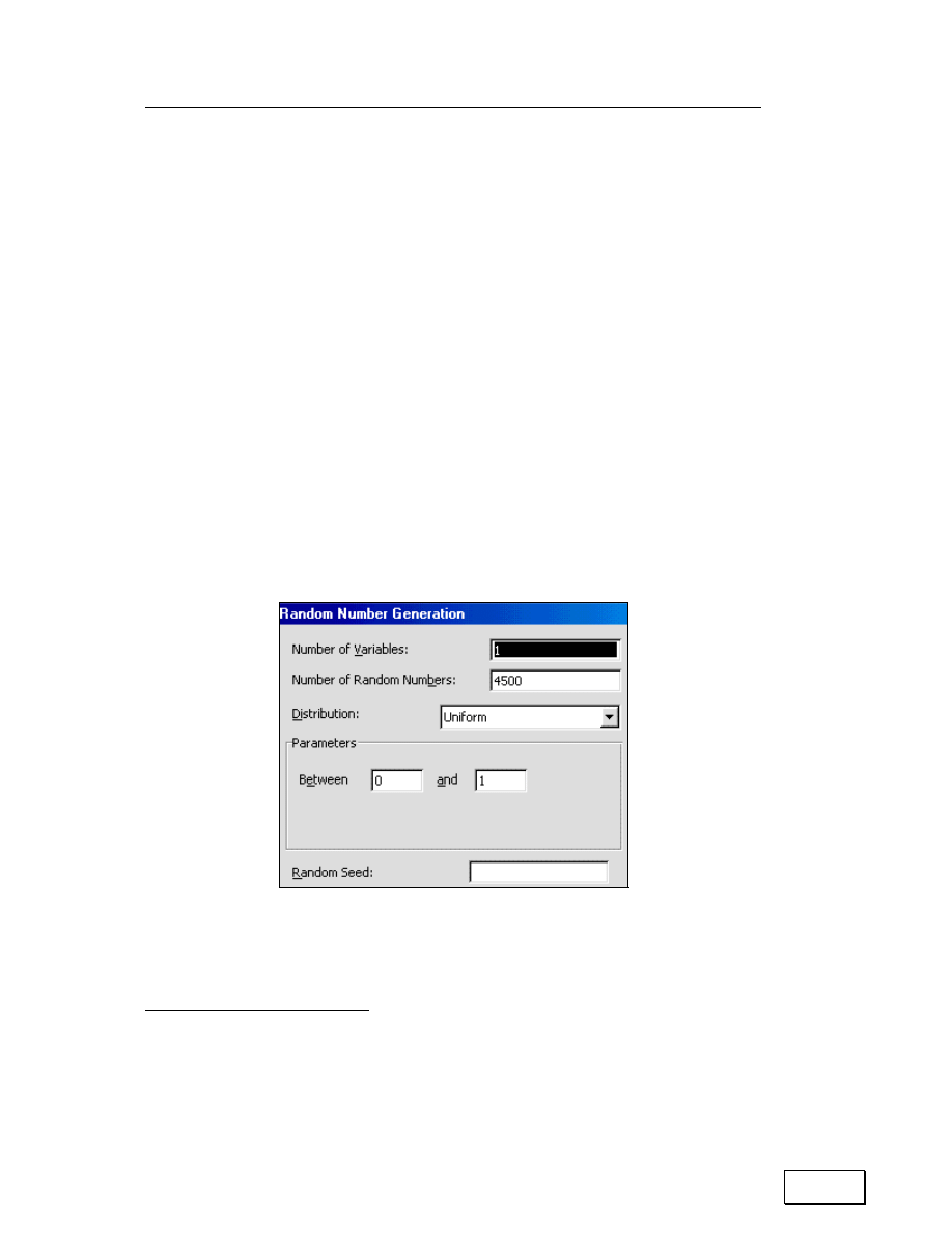
Statistical Analysis with Excel
230
13.2
RANDOM NUMBER GENERATION
This tool fills a range with independent random numbers drawn from one
of several Density Functions.
You can characterize a population with a Probability Density Function.
Select the option TOOLS/DATA ANALYSIS
34
and choose the procedure
“
Random Number Generation.”
Number of Variables: Number of columns of values you want in the output
table. If you do not enter a number, all columns in the output will be
filled.
Figure 158: Random Number Generator
34
If you do not see this option, then use TOOLS / ADD-INS to activate the Add-In for
data analysis. Refer to section 41.4.
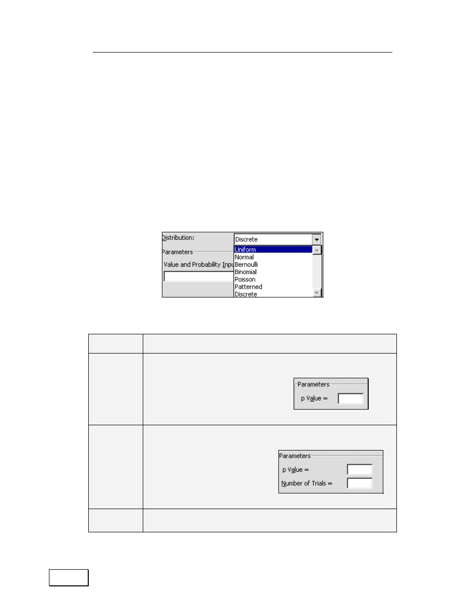
Chapter 13: Other Tools for Statistics
231
Number of Random Numbers: Number of data points you want to see.
Each point appears in a row of the output table. If you do not enter a
number, all rows in the output range will be filled.
Distribution: choose the Density Function for defining the criterion for the
Random Number generation.
Parameters: The base parameters for the generation process using the
selected Density Function.
Figure 159: Choice of Density Functions
Table 39: Choice of Density Functions
Distribution
Comment on setting parameters for random number generation
Bernoulli
This Density Function is
characterized by a probability of
success (p value) on any given
trial/observation.
Figure 160: Bernoulli
Binomial
This Density Function is
characterized by a probability of
success (p value) in any one
trial for a number of trials.
Figure 161: Binomial
Discrete
Figure 163: Discrete Or Custom
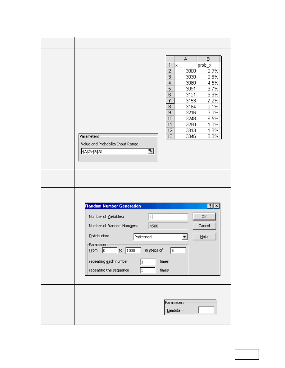
Statistical Analysis with Excel
232
Distribution
Comment on setting parameters for random number generation
Or Custom
Density
Function
The range must contain two
columns: The left column contains
values, and the right column
contains probabilities associated
with the value in that row. The
sum of the probabilities must be 1.
Note: You can use the function
FREQUENCY (A1, A:A)/count
(A:A) to generate the probability
you see in column B.
Figure 162: Parameters
Density Function
Normal
This Density Function is characterized by a mean and a standard
deviation.
Patterned
Figure 164: Patterned
Poisson
This Density Function is
characterized by a value
lambda, equal to (1/mean).
Figure 165: Poisson

Chapter 13: Other Tools for Statistics
233
Distribution
Comment on setting parameters for random number generation
Uniform
This distributing is characterized by lower and upper bounds.
Excel draws variables from all values in the range. The
probability of drawing a value is equal for all values in the range.
13.3
TIME SERIES
Exponential Smoothing
This tool and its formula predict a value based on the forecast for the
prior period, adjusted for the error in that prior forecast. The tool uses
the smoothing constant alpha, the magnitude of which determines how
strongly forecasts respond to errors in the prior forecast.
Using the mouse, select the menu path TOOLS/DATA ANALYSIS
35
and
choose the procedure
“
Exponential Smoothing.”
Damping: The factor you want to use as the exponential smoothing
constant. The damping factor is a corrective factor that minimizes the
instability of data collected across a population.
The default value for the damping factor is 0.3. Values of 0.2 to 0.3 are
reasonable smoothing constants. These values indicate that the current
forecast should be adjusted 20 to 30 percent for error in the prior forecast.
35
If you do not see this option, then use TOOLS / ADD-INS to activate the Add-In for
data analysis. Refer to section 41.4.
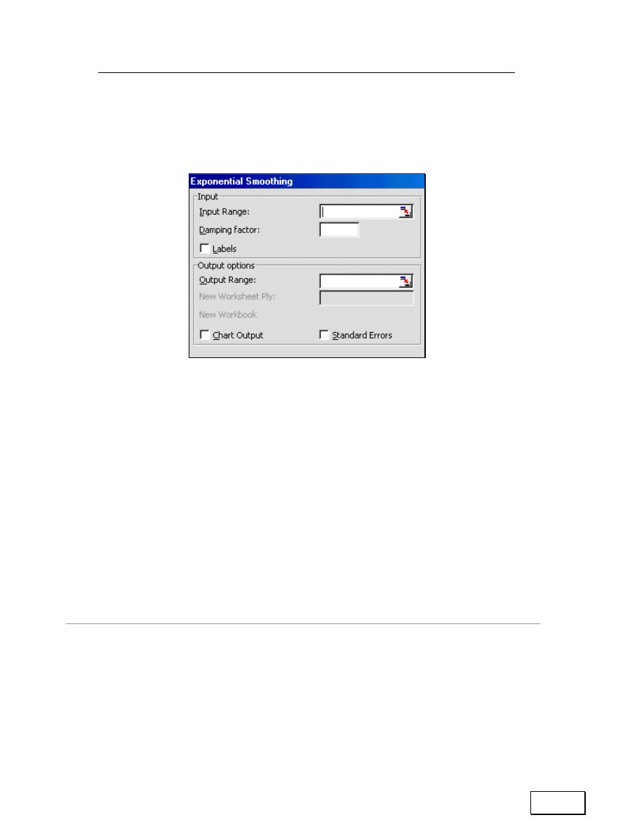
Statistical Analysis with Excel
234
Larger constants yield a faster response but can produce erratic
projections. Smaller constants can result in long lags for forecast values.
Figure 166: Exponential Smoothing
Data Requirement: A single column or row with four or more cells with
valid data.
Output: The output range must be on the same worksheet as the data in
the input range. Enter the range reference for the upper— left cell of the
output table (for example,
“
AD4”). You can obtain a column of Standard
Errors by selecting the option
“
Standard Errors.” If you want to chart the
procedure's output — the actual values and forecasts –, select the option
“
Chart Output.”
Moving Average analysis
This tool projects values in the forecast period based on
“
the average
value of the series over a specific number of preceding periods.” A moving
average provides trend information that a simple average of all historical
data would mask.
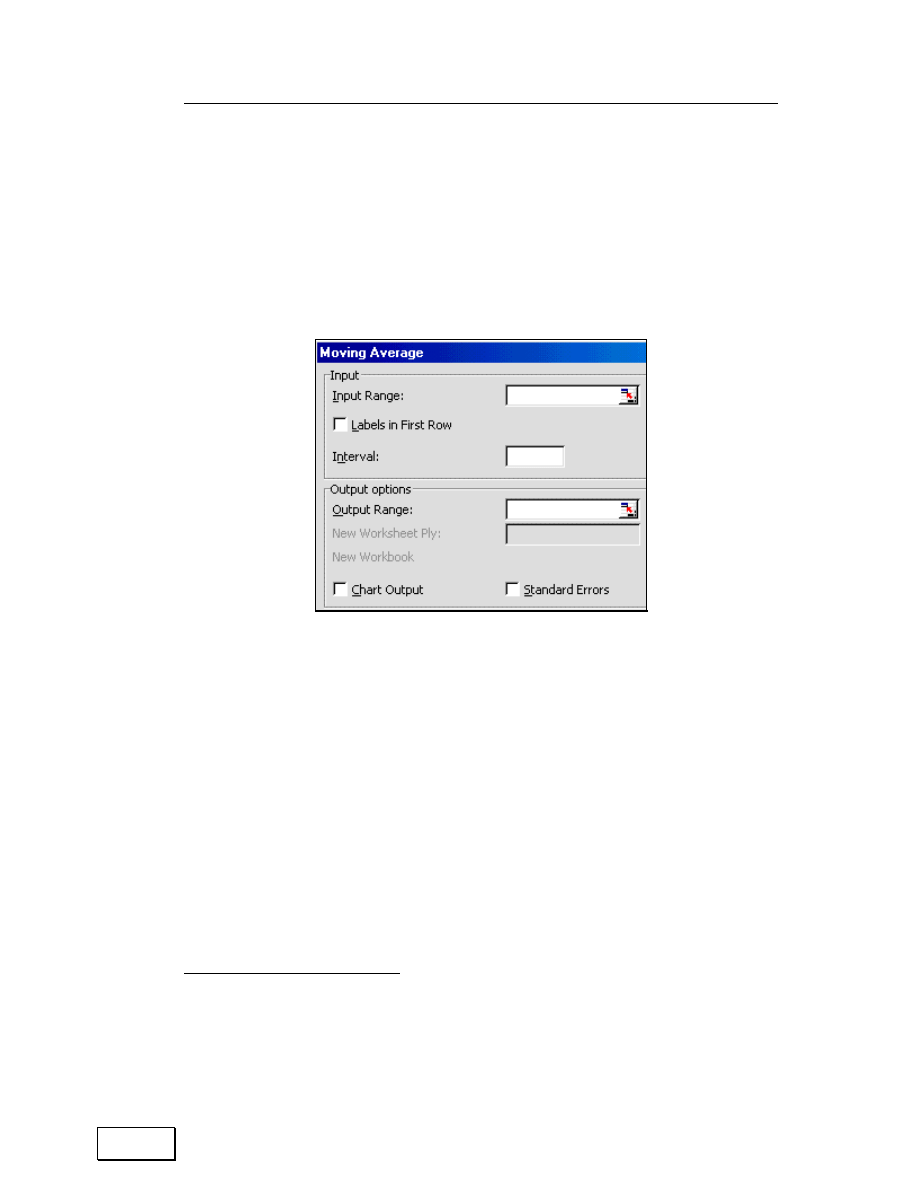
Chapter 13: Other Tools for Statistics
235
Select the option TOOLS/DATA ANALYSIS
36
and choose the procedure
“
Moving Average.”
Interval: Number of values you want to include in the moving average.
The default is three.
Figure 167: Moving Average
Data Requirement: A single column or row with four or more cells with
valid data.
Output: The output range must be on the same worksheet as the data in
the input range. Enter the range reference for the upper–left cell of the
output table (for example,
“
AD4”). You can obtain a column of Standard
Errors by selecting the option
“
Standard Errors.” If you want to chart the
procedure's output — the actual values and forecasts –, select the option
36
If you do not see this option, then use TOOLS / ADD-INS to activate the Add-In for
data analysis. Refer to section 41.4.

Statistical Analysis with Excel
236
“
Chart Output.”

Page for Notes

Statistical Analysis with Excel
238
CHAPTER 14
THE SOLVER TOOL FOR CONSTRAINED LINEAR
OPTIMIZATION
This chapter teaches:
— DEFINING THE OBJECTIVE FUNCTION (CHOOSING THE
OPTIMIZATION CRITERION)
— ADDING CONSTRAINTS
— OPTIONS
14.1
DEFINING THE OBJECTIVE FUNCTION (CHOOSING
THE OPTIMIZATION CRITERION)
The problem of constrained optimization:
For example,
Maximize/Minimize /other (over the choice parameters Xc …) Y = f(X1, X2 …)
Subject to the inequality constraints:-
C1 = ….C2 >=… , C3 <= …
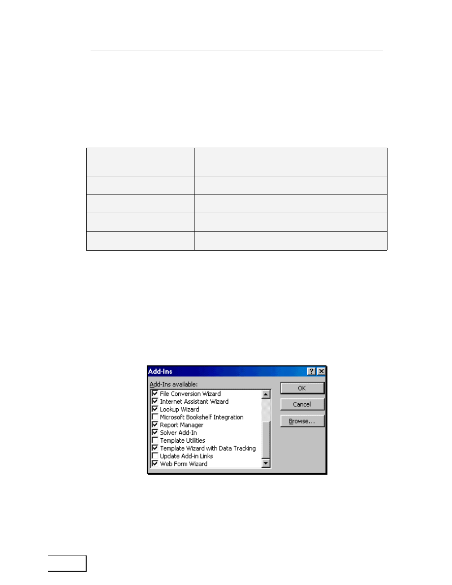
Chapter 14: The Solver Tool for Constrained Optimization
239
The Add-In
“
Solver” can solve such models. In the Solver dialog (user-
input form), the options equate with the function above. The
“
mapping” of
the dialog to different parts of the optimization function is shown in the
next table.
Table 40: The “Solver”
Option in the Solver dialog
….
Equate to the following part of the optimization
function…
Equal to:”
The optimization function
Set Target Cell”
Function that needs to be optimized
By Changing Cells”
The choice parameters Xc….
Subject to the Constraints” The constraints C1, C2, …
The Solver permits constraints of inequality. This makes the solver
extremely powerful.
Choose the menu option TOOLS/ADD-INS. Choose the Add-In
“
Solver” as
shown in Figure 168. Execute the dialog by clicking on the button OK.
Figure 168: Selecting the Solver Add-In

Statistical Analysis with Excel
240
You have activated the
“
Analysis ToolPak.” If you go to the menu
TOOLS, you will see the option
“
SOLVER“— this option was not there
before you accessed the Add-In. Please define a sample problem and try it
on an Excel workbook
37
.
Access the feature through the menu path TOOLS/SOLVER. The dialog
shown in Figure 169 opens. The
“
Target Cell” contains the formula for
the function you are attempting to optimize.
The
“
Equal to” area is where you choose the optimization criterion–
— Maximization (Max)
— Minimization (Min)
37
I do not supply the sample data for most of the examples in chapter 42 to chapter 46.
My experience is that many readers glaze over the examples and do not go through
the difficult step of drawing inferences from a result if the sample data results are
the same as those in the examples in the book.
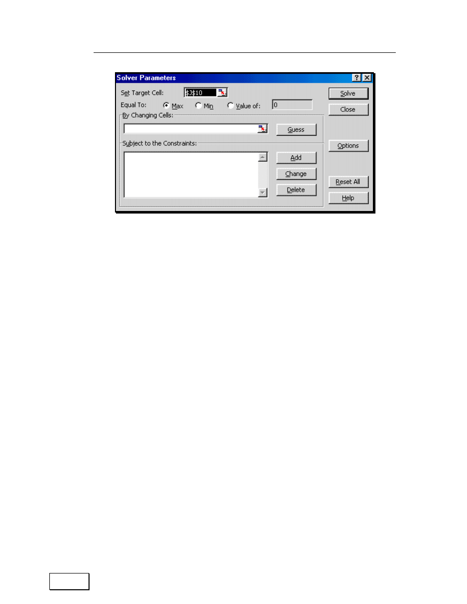
Chapter 14: The Solver Tool for Constrained Optimization
241
Figure 169: Setting the target cell
The choice parameters are the numbers the algorithm plays around with
to find the max/min.
You have to tell Excel about the cells that contain these parameters. One
can do it manually, or, an easier option is to click on the button
“
Guess.”
Excel automatically chooses all the cell references for use in the formula
in J10 (the target cell/objective function). This is illustrated in Figure
170.
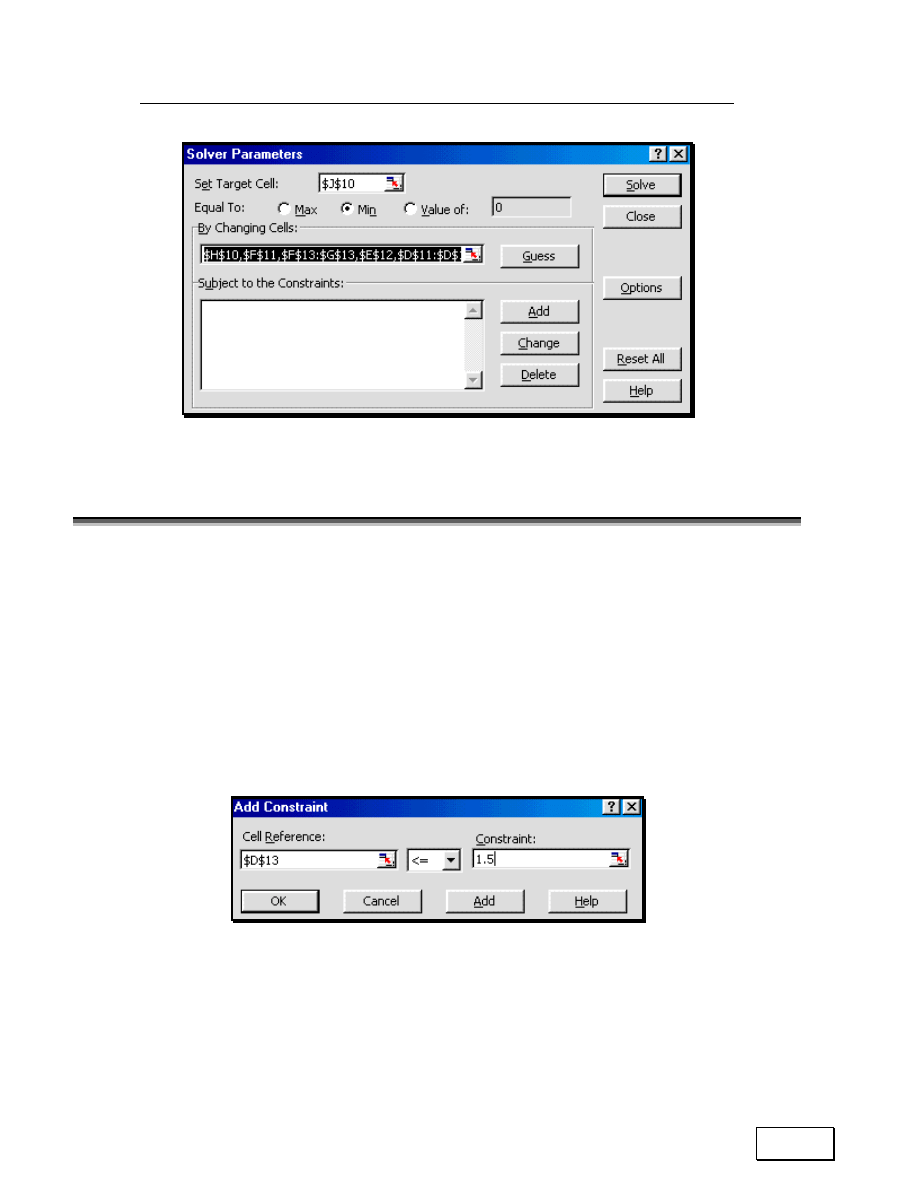
Statistical Analysis with Excel
242
Figure 170: Selecting the criterion for optimization
14.2
ADDING CONSTRAINTS
The optimization function has been defined, as have the
“
choice
parameters.” At this stage, you have to add the constraints.
Click on the button
“
Add” and write in a constraint as shown in Figure
171.
Figure 171: The first constraint
After defining the first constraint, click on the button
“
Add” (see Figure
171.) Write the second constraint— see Figure 172.
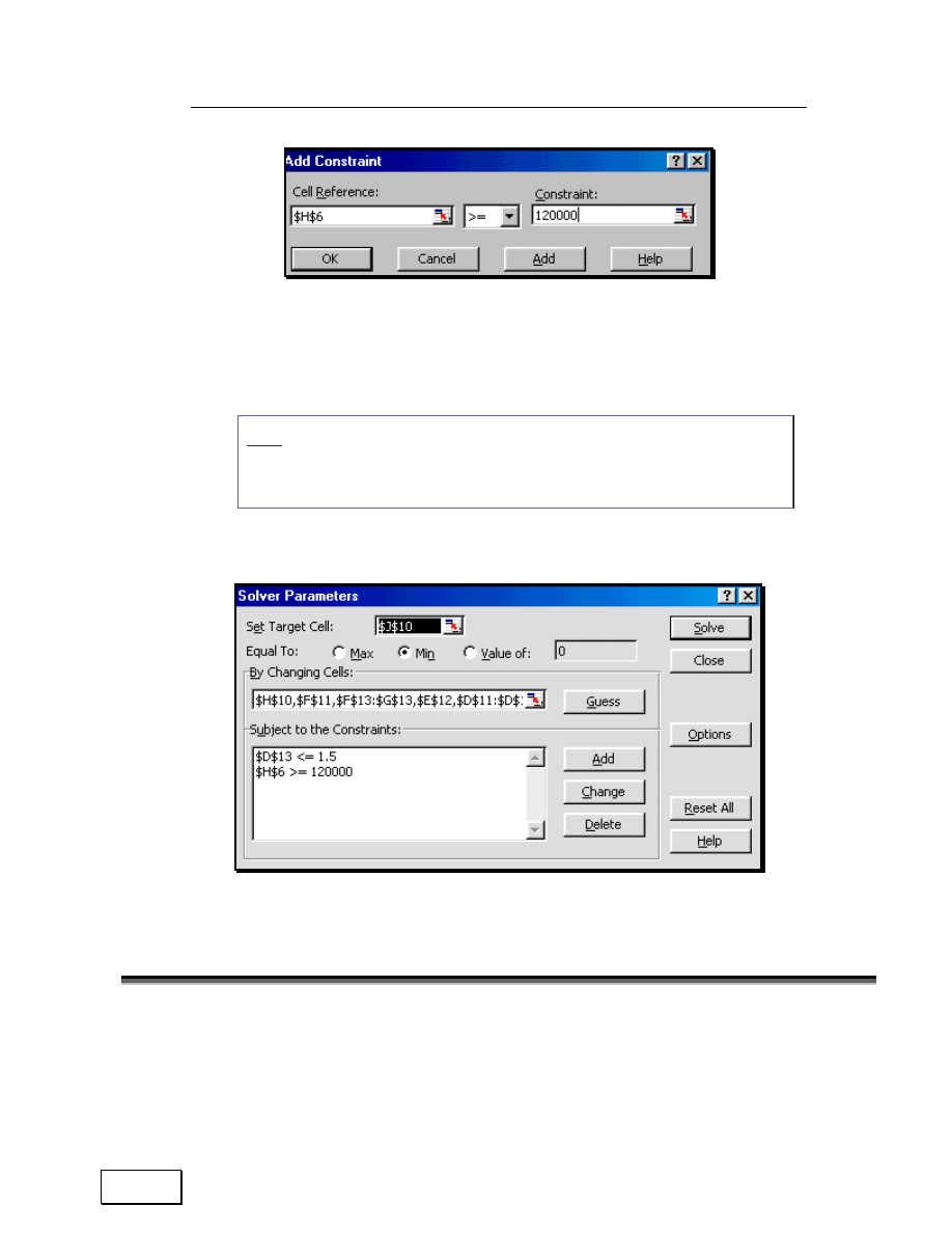
Chapter 14: The Solver Tool for Constrained Optimization
243
Figure 172: The second constraint
Continue with constraint definitions. After defining the last constraint,
execute the dialog by clicking on the button OK (see Figure 172).
Note:
The constraints are shown in the area “Subject to the Constraints” as
shown in Figure 173.
Figure 173: The constraints for the Solver
14.3
CHOOSING ALGORITHM OPTIONS
You need to choose the options for the analysis. So, click on the button
“
Options.” The dialog shown in Figure 174 opens.
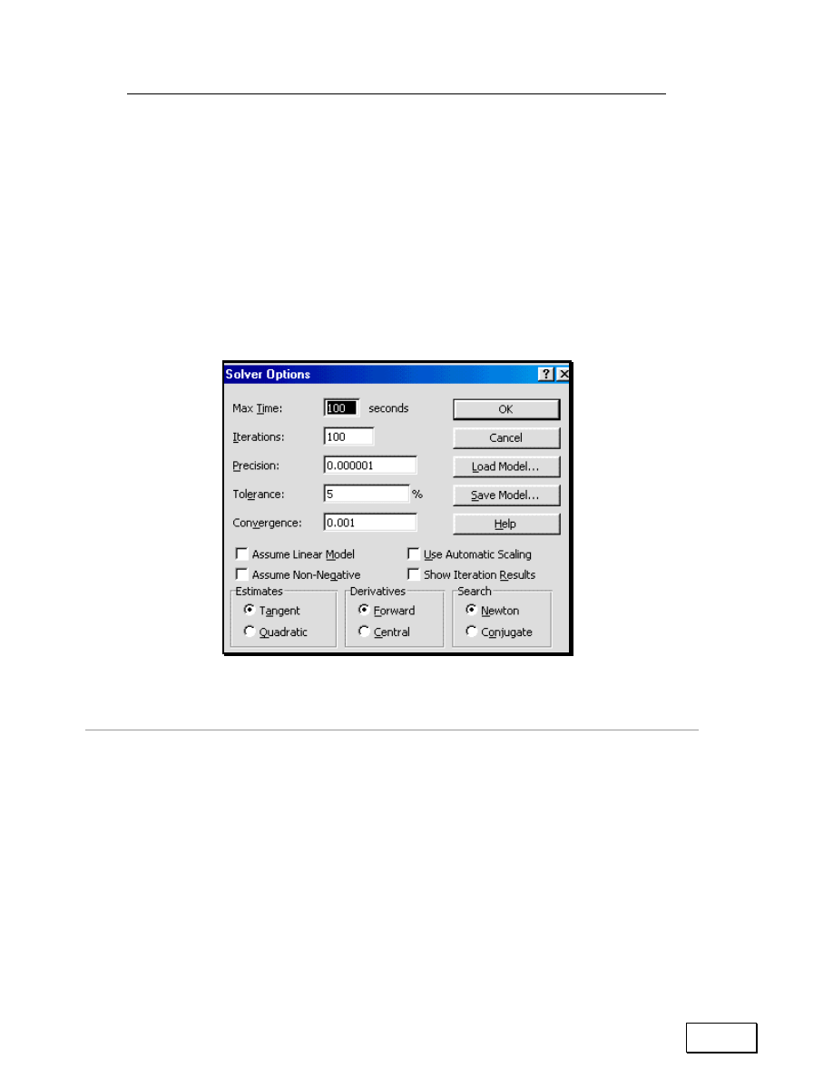
Statistical Analysis with Excel
244
You may want to increase the iterations to 10,000. If you want to relax
the requirements for preciseness, increase the value of
“
Precision” by
removing some post-decimal zeros.
“
Save Model” is used to save each optimization model. You can define
several optimization problems in one workbook. The other options are
beyond the scope of this book. Click on the button
“
Continue.”
Figure 174: Options in the Solver Add-In
Running the Solver
Execute the procedure by clicking on the button
“
Solve.”
The following output can be read from the spreadsheet.
• the optimized value of the Objective Function (that is, the value of
the formula in the cell defined in the box
“
Set Target Cell”)
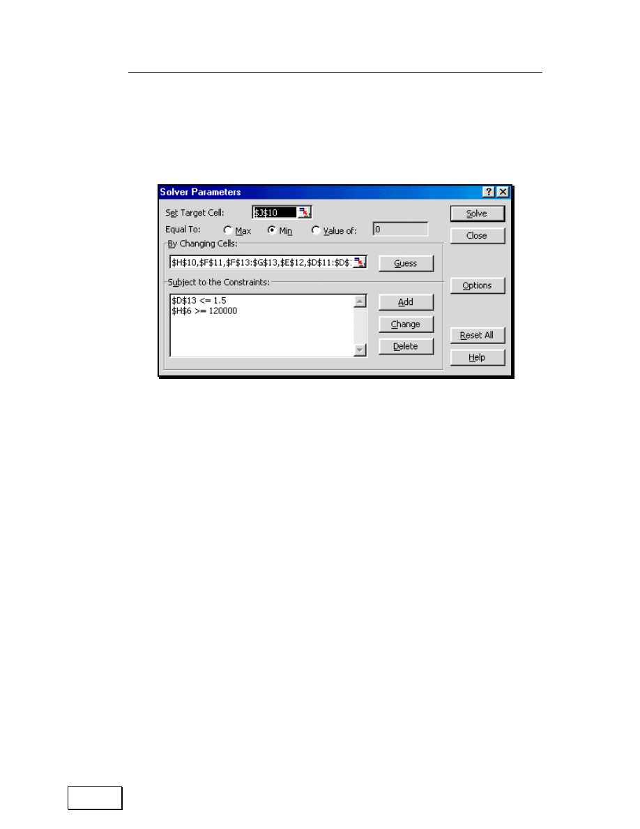
Chapter 14: The Solver Tool for Constrained Optimization
245
•
is the combination of the choice variables (that is, those whose
value is obtained from the cells defined in the dialog area
“
By
Changing Cells”)
Figure 175: The completed constrained optimization dialog

Statistical Analysis with Excel
246
INDEX
#
µ 122
σ2 122
A
A1................................................ 25, 28, 232
ABS.........................................................153
ADD–IN..................................................161
ADD-INS . 17, 161, 163, 165, 170, 176, 178,
187, 190, 195, 199, 205, 219, 231, 234,
236, 240
ADD–INS INSTALLED WITH EXCEL161
AND.................... 35, 52, 109, 144, 161, 169
ANOVA . 129, 156, 163, 183, 187, 203, 205,
206, 207, 208
AUDITING........... 17, 76, 78, 79, 80, 81, 84
AUTOCORRECT .....................................17
AUTOFORMAT.......................................16
AVEDEV ........................................156, 157
AVERAGE....................66, 89, 90, 106, 155
AVERAGEA...........................................106
B
BETADIST .............113, 115, 132, 140, 141
BETAINV .......................133, 134, 140, 141
BINOMDIST...................................113, 140
BIVARIATE ...........................................169
C
CDF 109, 110, 111, 112, 113, 114, 115, 119,
120, 121, 123, 125, 127, 128, 129, 130,
132, 133, 134, 136, 137, 138, 140
CELL.............................................25, 52, 89
CELL REFERENCE .................................25
CELLS...........................................15, 16, 52
CENTRAL TENDENCY ..........................89
CHIDIST .........113, 115, 130, 131, 140, 141

Index
247
CHIINV .................................. 131, 140, 141
CHI-SQUARE DENSITY FUNCTION. 109
CHOOSE ................................................ 153
CLEAR..................................................... 14
COLUMN........................................... 16, 52
COLUMNS......................................... 15, 52
COMMENT.............................................. 16
COMMENTS ............................... 14, 35, 52
CONDITIONAL FORMATTING............ 16
CONFIDENCE......................69, 70, 71, 109
CONFIDENCE INTERVAL.................. 109
CONSOLIDATION.................................. 17
CONSTRAINTS..................................... 239
CONTROLLING CELL REFERENCE
BEHAVIOR WHEN COPYING AND
PASTING FORMULAE (USE OF THE
............................................................. 35
COPY ..........................13, 36, 37, 38, 39, 42
COPYING AND PASTING............... 35, 36
COPYING AND PASTING A FORMULA
TO OTHER CELLS IN A DIFFERENT
ROW AND COLUMN ........................ 35
COPYING AND PASTING A FORMULA
TO OTHER CELLS IN THE SAME
COLUMN ............................................ 35
COPYING AND PASTING A FORMULA
TO OTHER CELLS IN THE SAME
ROW .................................................... 35
COPYING AND PASTING FORMULAS
FROM ONE WORKSHEET TO
ANOTHER........................................... 35
CORREL..................................... 67, 68, 157
CORRELATION ............ 144, 169, 179, 180
COS......................................... 81, 82, 83, 84
COUNT................... 106, 144, 145, 146, 147
COUNTA................................ 106, 144, 147
COUNTBLANK............................. 144, 148
COUNTIF ....................... 144, 151, 152, 153
COUNTING AND SUMMING.............. 144
COVAR .................................................. 157
COVARIANCE ...................................... 144
CROSS SERIES RELATIONS .............. 144
CUMULATIVE DENSITY FUNCTION109
CUSTOMIZE............................................ 17

Statistical Analysis with Excel
248
CUT ....................................................13, 49
CUTTING AND PASTING FORMULAE
..............................................................35
D
DATA ANALYSIS 170, 171, 173, 176, 178,
187, 190, 195, 199, 205, 219, 229, 231,
234, 236
DATE........................................................80
DEGREES.................................................83
DELETE SHEET ......................................14
DESCRIPTIVE STATISTICS ................169
DEVIATIONS FROM THE MEAN.......144
DEVSQ ...................................................156
DISPERSION ...........................................89
E
EDIT .. 13, 36, 37, 38, 39, 40, 42, 49, 53, 54,
56, 57, 58, 59
EXP.........................................................154
EXPONDIST .................. 113, 136, 137, 140
EXPONENTIAL..................... 109, 144, 229
EXPONENTIAL SMOOTHING ............229
EXTERNAL DATA..................................17
F
FALSE.............100, 101, 137, 145, 146, 148
FDIST......................113, 115, 129, 140, 141
FILE ....................................................13, 53
FILL ..........................................................14
FILTER .....................................................17
FIND .........................................................14
FINV .......................................130, 140, 141
FISHER ...................................................109
FORM .......................................................17
FORMAT ..................................................16
FORMULA14, 25, 27, 35, 52, 61, 76, 81, 84
FORMULA BAR ................................14, 27
FREEZE PANES.......................................18
FREQUENCY.........................................232
F-TESTING FOR EQUALITY IN
VARIANCES .....................................183

Index
249
FUNCTION....15, 61, 62, 63, 67, 69, 71, 72,
89, 90, 91, 92, 93, 95, 96, 97, 99, 100,
104, 105, 109, 120, 121, 123, 124, 125,
126, 129, 131, 132, 133, 134, 135, 136,
145, 147, 148, 149, 151, 152, 155, 158,
159, 161, 225
FUNCTION / FINANCIAL ..................... 15
FUNCTION / INFORMATION ....... 15, 148
FUNCTION / LOGICAL ......................... 15
FUNCTION / LOOKUP........................... 15
FUNCTION / MATH & TRIG................. 15
FUNCTION / STATISTICAL15, 91, 92, 93,
95, 96, 97, 99, 100, 101, 104, 105, 120,
121, 123, 124, 125, 126, 129, 131, 132,
133, 134, 135, 136, 145, 147, 152, 155,
225
FUNCTION / TEXT................................. 15
FUNCTION WITHIN A FUNCTION ..... 61
FUNCTIONS ENDING WITH AN ......... 89
G
GAMMADIST ................113, 134, 135, 140
GAMMAINV ......................... 135, 136, 140
GEOMEAN .............................................. 93
GEOMETRIC MEAN .............................. 89
GO TO ...................................................... 14
GOAL SEEK .................................... 17, 241
GROUP AND OUTLINE ......................... 17
H
H0 ...184, 185, 186, 190, 193, 194, 196, 197,
198, 200, 201, 202, 205
HARMEAN .............................................. 92
HARMONIC MEAN................................ 89
HEADER .................................................. 14
HEADER AND FOOTER ........................ 14
HELP ........................................................ 18
HIDE......................................................... 18
HYPERLINK............................................ 16
HYPGEOMDIST............................ 113, 140
I
IF 144, 153

Statistical Analysis with Excel
250
INSERT ... 15, 44, 46, 47, 61, 63, 67, 69, 71,
72, 90, 91, 92, 93, 95, 96, 97, 99, 100,
104, 105, 120, 121, 123, 124, 125, 126,
129, 131, 132, 133, 134, 135, 136, 145,
147, 148, 149, 151, 152, 153, 155, 158,
159, 225
INVERSE MAPPING.............................109
K
KURT......................................................105
KURTOSIS...............................................89
L
LARGE ...............................................89, 98
LINKS.......................................................14
LN ...........................................................154
LOG ........................................ 115, 144, 155
LOG10 ....................................................154
LOGINV ......................................... 140, 141
LOGNORMDIST............ 113, 115, 140, 141
M
MACROS..........................................17, 161
MAX ...........................................97, 98, 106
MAXA.........................................97, 98, 106
MEDIAN.............................................89, 95
MIN...................................................98, 106
MINA ................................................98, 106
MODE...........................................84, 89, 95
MOVE OR COPY SHEET........................14
MOVING AVERAGE ............................229
MULTIPLE RANGE REFERENCES ......61
MULTIPLYING/DIVIDING/SUBTRACTI
NG/ADDING ALL CELLS IN A
RANGE BY A NUMBER....................52
N
N 136, 146, 174, 214
NA...................................15, 44, 47, 83, 146
NEGBINOMDIST ..........................113, 140
NORMAL DENSITY FUNCTION 109, 144
NORMDIST....113, 115, 119, 120, 140, 141

Index
251
NORMINV ......................122, 123, 140, 141
NORMSDIST ..........113, 115, 123, 140, 141
NORMSINV................................... 140, 141
NOT............................................ 35, 52, 161
O
OBJECT ............................................. 14, 16
OBJECTIVE FUNCTION...................... 239
OFFICE ASSISTANT.............................. 18
OFFICE CLIPBOARD............................. 14
ONLINE COLLABORATION ................ 17
OPEN........................................................ 13
OPTIMIZATION.................................... 239
OPTIMIZATION CRITERION ............. 239
OPTIONS ..........................17, 26, 28, 35, 52
OR ............................................................ 89
P
PAGE BREAK ................................... 14, 15
PAGE BREAK PREVIEW....................... 14
PAGE SETUP .......................................... 13
PAIRED SAMPLE T-TEST ................... 183
PASTE 13, 14, 35, 36, 37, 38, 40, 47, 49, 53,
54, 56, 57, 58, 62
PASTE SPECIAL ....... 14, 53, 54, 56, 57, 58
PASTING ALL BUT THE BORDERS.... 52
PASTING COMMENTS .......................... 52
PASTING DATA VALIDATION............ 52
PASTING ONLY FORMATS.................. 52
PASTING ONLY THE FORMULA .. 35, 52
PASTING THE RESULT OF A
FORMULA, BUT NOT THE
FORMULA ITSELF ............................ 35
PDF.109, 110, 112, 113, 119, 121, 127, 133,
134, 136, 137, 138, 140
PEARSON .............................................. 157
PERCENTILE ...................... 89, 96, 97, 169
PERCENTRANK ..................................... 99
PIVOT REPORT ...................................... 17
POISSON........................ 109, 113, 138, 140
PRECEDENTS ......................................... 76
PRINT AREA........................................... 13
PRINT PREVIEW .................................... 13

Statistical Analysis with Excel
252
PROBABILITY DENSITY FUNCTION109
PRODUCT...................................... 144, 149
PROPERTIES ...........................................13
PROTECTION..........................................16
Q
QUARTILE.........................................89, 96
R
R1C1 ...................................................25, 28
RANDOM NUMBER GENERATION ..229
RANK ....................................... 89, 100, 169
REDO........................................................13
REFERENCES ALLOWED IN A
FORMULA ..........................................25
REFERENCING A BLOCK OF CELLS..25
REFERENCING CELLS FROM
ANOTHER WORKSHEET .................25
REFERENCING CORRESPONDING
BLOCKS OF CELLS / ROWS /
COLUMNS FROM A SET OF
WORKSHEETS...................................25
REFERENCING ENTIRE COLUMNS....25
REFERENCING ENTIRE ROWS............25
REFERENCING NON– ADJACENT
CELLS..................................................25
REGRESSION ........................................211
REPLACE .................................................14
ROW ...................................................16, 52
ROWS .................................................15, 52
ROWS TO COLUMNS.............................52
RSQ.........................................................157
S
SAMPLING ANALYSIS........................229
SAVE ........................................................13
SAVE AS ..................................................13
SAVE AS WEB PAGE .............................13
SAVE WORKSPACE...............................13
SCENARIOS.............................................17
SEARCH ...................................................13
SHARE WORKBOOK .............................16
SHEET ......................................................16

Index
253
SIGN................................................. 35, 153
SKEW..................................................... 104
SKEWNESS ............................................. 89
SMALL .................................................... 99
SOLVER......................................... 239, 241
SORT........................................................ 17
SPEECH ................................................... 16
SPELLING ............................................... 16
SPLIT ....................................................... 18
SPSS ............................................... 3, 5, 170
SQRT...................................................... 153
STANDARD DEVIATION...................... 89
STANDARD NORMAL OR Z– DENSITY
FUNCTION ....................................... 109
STANDARDIZE ............................ 155, 225
STATA ....................................................... 5
STATUS BAR.......................................... 14
STDEV ..........71, 72, 89, 100, 101, 106, 155
STDEVA ...................89, 100, 101, 102, 106
STDEVP................................... 89, 101, 106
STDEVPA ................................ 89, 101, 106
STYLE................................................ 16, 25
SUBTOTALS ........................................... 17
SUM.................................. 33, 144, 145, 148
SUM OF THE SQUARES OF
DIFFERENCES ACROSS TWO
VARIABLES ..................................... 145
SUM OF THE SUM OF THE SQUARES
OF TWO VARIABLES ..................... 144
SUMIF ............................ 144, 150, 151, 153
SUMPRODUCT ............................. 144, 149
SUMX2MY2 .................................. 158, 159
SUMX2PY2.................................... 157, 158
SUMXMY2 ............................................ 158
T
T 23, 109, 115, 119, 125, 126, 127, 128,
163, 183, 189, 192, 193, 194, 195, 196,
197, 198, 199, 200, 201, 202, 203, 204,
205, 218, 223
T– DENSITY FUNCTION..................... 109
TABLE ............................................... 17, 50
TDIST ..................... 113, 115, 125, 140, 141

Statistical Analysis with Excel
254
TIME................................................. 36, 229
TIME SERIES ........................................229
TINV....... 121, 124, 126, 127, 128, 140, 141
TOOLBARS .......................................14, 80
TOOLS16, 17, 26, 28, 76, 78, 79, 80, 81, 84,
163, 165, 170, 171, 173, 176, 178, 187,
190, 195, 199, 205, 219, 229, 231, 234,
236, 240, 241
TRACE ...............................................76, 78
TRACING THE CELL REFERENCES
USED IN A FORMULA......................76
TRACING THE FORMULAS IN WHICH
A PARTICULAR CELL IS
REFERENCED ....................................76
TRIMMEAN................................. 91, 92, 94
TRIMMED MEAN...................................89
TRUE .............. 100, 101, 137, 145, 146, 148
T-TEST
TWO– SAMPLE ASSUMING
EQUAL VARIANCES
.............. 183
TWO– SAMPLE ASSUMING
UNEQUAL VARIANCES
........ 183
T-TESTING MEANS WHEN THE TWO
SAMPLES ARE FROM DISTINCT
GROUPS ............................................183
U
UNDO ...........................................13, 49, 59
V
VALIDATION ..........................................17
VALUE .............................................89, 146
VAR ..........................................89, 100, 106
VARA ...............................89, 100, 101, 106
VARIANCE ..............................................89
VARP ........................................89, 101, 106
VARPA .....................................89, 101, 106
VIEW ......................................14, 26, 27, 80
W
WEB..........................................................17
WEIBULL.......................109, 113, 138, 140
WINDOW .....................................18, 76, 80
WORKSHEETS ..................................15, 36

Index
255
Z
ZOOM ...................................................... 15
Z-TESTING FOR POPULATION MEANS
........................................................... 183

Statistical Analysis with Excel
256
VJ Inc Corporate and Government Training
We provide productivity-enhancement and capacity building for
corporate, government, and other clients. The onsite training includes
courses on:
Office Productivity Software and Tools
Data Mining, Statistics, Forecasting, Econometrics
Financial Analysis, Feasibility Studies
Risk Analysis, Monitoring and Management
Building and using Credit Rating/Monitoring Models
Specific software applications, including Microsoft Excel, VBA, Word,
PowerPoint, Access, Project, SPSS, SAS, STATA, ands many other
Contact our corporate training group at http://www.vjbooks.net.
Wyszukiwarka
Podobne podstrony:
Kurs Excel`a, Lekcja 01, Lekcja 1 - Tworzenie nowego skoroszytu i zapisywanie
Kurs Excel`a, Lekcja 12, Lekcja 12 - drukowanie specjalne
Kurs Excel`a, Lekcja 10, Lekcja 10 - hasła w Excel'u
Kurs EXCEL
Kurs Excel`a, Lekcja 07, Lekcja 7 - kopiowanie, wycinanie i wklejanie (odwołania)
Kurs Excel`a, Lekcja 03, Lekcja 3 - edycja danych
KURS EXCEL podstawowy
kurs excel exel 2000 deutsch JZBZHKXJPX32CEXKUA2LVK7EEZG36RUGIJPBA7A
podstawowy kurs excel 2007, Informatyka
Kurs Excel`a, Lekcja 09, Lekcja 9 - drukowanie
więcej podobnych podstron