
Rahul Chacko
IB Mathematics HL Revision – Step One
Chapter 1.1 – Arithmetic sequences and series; sum of finite arithmetic series; geometric
sequences and series; sum of finite and infinite geometric series. Sigma notation.
Arithmetic Sequences
Definition: An arithmetic sequence is a sequence in which each term differs from the
previous one by the same fixed number:
{u
n
} is arithmetic if and only if
d
u
u
n
n
1
.
Information Booklet
d
n
u
u
n
1
1
Proof/Derivation:
d
u
u
n
n
1
d
u
u
n
n
1
dn
u
u
n
1
1
dn
u
u
n
1
d
n
u
u
n
1
1
Derivations:
d
n
u
u
n
1
1
1
1
n
u
u
d
n
1
1
d
u
u
n
n
Information Booklet
n
n
u
u
n
d
n
u
n
S
1
1
2
1
2
2
Proof:
S
n
= u
1
+ u
2
+ u
3
+ …+ u
n
= u
1
+ (u
1
+ d) + (u
1
+ 2d) + (u
1
+ 3d) + …+ (u
1
+ (n − 1)d)
= u
n
+ (u
n
− d) + (u
n
− 2d) + (u
n
+ 3d) + …+ (u
n
− (n − 1)d)
2S
n
= n(u
1
+ u
n
)
n
n
u
u
n
S
1
2
Derivations

1
2
u
n
S
u
n
n
n
n
u
n
S
u
2
1
n
n
u
u
S
n
1
2
Geometric Sequences
Definition: A geometric sequence is a sequence in which each term can be obtained from
the previous one by multiplying by the same non-zero constant.
{u
n
} is geometric if and only if
,
1
r
u
u
n
n
n
where r is a constant.
Information Booklet
1
1
n
n
r
u
u
Proof:
r
u
u
n
n
1
r
u
u
n
n
1
n
n
r
u
u
1
1
1
1
n
n
r
u
u
Derivations:
1
1
n
n
r
u
u
1
1
1
n
n
u
u
r
1
log
1
u
u
n
n
r
(non-calculator paper)
1
log
log
1
r
u
u
n
n
(calculator paper)
Compound Interest:
n
n
r
u
u
1
1
, where
1
u
initial investment,
%
100
%
%
100
i
r
,
i interest rate per
compounding period,
n = number of periods and
1
n
u
amount after
n periods.
1
n
n
u
r
u

Information Booklet
r
r
u
r
r
u
S
n
n
n
1
1
1
1
1
1
,
r
1
Proof:
S
n
=
u
1
+
u
2
+ u
3
+ …+ u
n-1
+
u
n
=
u
1
+
u
1
r + u
1
r
2
+
u
1
r
3
+ … +
u
1
r
n−2
+
u
1
r
n−1
rS
n
= (
u
1
r + u
1
r
2
+
u
1
r
2
+
u
1
r
3
+
u
1
r
4
+ … +
u
1
r
n−1
) +
u
1
r
n
rS
n
= (
S
n
−
u
1
) +
u
1
r
n
rS
n
−
S
n
=
u
1
r
n
−
u
1
S
n
(
r − 1) = u
1
(
r
n
− 1)
1
1
1
r
r
u
S
n
n
Derivations
1
1
1
n
n
r
r
S
u
r
u
S
r
n
n
log
1
log
1
1
2
3
3
2
1
...
1
1
1
n
n
n
n
n
r
r
r
r
r
r
r
r
u
S
Sum to infinity
r
u
S
1
1
,
1
r
Proof:
r
r
u
S
n
n
1
1
1
,
1
r
,
0
r
,
1
r
r
u
S
1
0
1
1
,
1
r
r
u
S
1
1
,
1
r
Sigma Notation
n
r
n
f
1
)
(

n is the number of terms, f(n) is the general term and r = the first n value in the sequence.
represents “the sum of” these the terms in this progression.
Chapter 1.2 – Exponents and logarithms. Laws of exponents; laws of logarithms.
Change of base.
Definition of Exponents:
y
x
a
means
x
y
a , i.e. the numerator in an exponent is the power
to which a number is raised and the denominator is the root to which it is lowered.
Laws of Exponents
xy
y
x
a
a
y
x
y
x
a
a
a
a
a
a
1
1
1
0
Definition of Logarithms:
y
x
a
log
means
x
a
y
.
Notes:
,
log
ln
x
x
e
where
e is the unique real number such that the function e
x
has the same
value as the slope of the tangent line, for all values of
x.
b
y
b
b
x
b
y
y
x
b
b
a
b
a
x
b
a
y
a
y
a
a
a
y
x
y
x
y
a
log
log
log
log
log
log
1
log
1
log
a
x
a
a
a
x
a
x
a
b
a
x
b
b
x
b
a
b
a
a
x
a
a
log
log
log
log
THEREFORE
x
x
a
a
a
x
a
log
log
Other Significant Equations
a
x
x
e
a
ln
Proof:

a
x
x
x
a
a
x
e
a
a
e
e
x
ln
ln
ln
Other Significant Equations
b
a
a
c
c
b
log
log
log
Proof:
b
a
a
b
a
x
a
b
x
a
b
a
b
x
a
c
c
b
c
c
c
c
c
x
c
x
b
log
log
log
log
log
log
log
log
log
log
Laws of Logarithms
b
a
ab
n
n
n
log
log
log
Proof:
b
a
ab
ab
x
ab
n
ab
n
a
b
n
a
n
n
a
n
b
x
a
x
b
a
n
n
n
n
n
x
n
x
x
b
x
b
x
n
n
n
n
n
n
log
log
log
log
log
log
log
log
log
log
log
log
Laws of Logarithms
b
a
ab
n
n
n
log
log
log
Proof:

b
a
b
a
b
a
x
b
a
n
b
a
n
a
bn
a
n
n
a
n
b
x
a
x
b
a
n
n
n
n
n
x
n
x
x
b
x
b
x
n
n
n
n
n
n
log
log
log
log
log
log
log
log
log
log
log
log
Chapter 1.3 – Counting principles, including permutations and combinations. The
binomial theorem: expansion of
,
n
b
a
n
.
The Product Principle
If there are m different ways of performing an operation and for each of these there are n
different ways of performing a second independent operation, then there are mn different
ways of performing the two operations in succession.
The number of different ways of performing an operation is equal to the sum of the
different mutually exclusive possibilities.
Factorial Notation
!
n
is the product of the first n positive integers for
1
n
.
1
!
0
!
0
1
)!
1
1
(
1
!
1
)!
3
)(
2
)(
1
(
)!
2
)(
1
(
)!
1
(
!
etc
n
n
n
n
n
n
n
n
n
n
Permutations (in a line)
A permutation of a group of symbols is any arrangement of those symbols in a definite
order
.
Explanation: Assume you have n different symbols and therefore n places to fill in your
arrangement. For the first place, there are n different possibilities. For the second place,
no matter what was put in the first place, there are
1
n
possible symbols to place, for the
r
th
place there are
1
r
n
possible places until the point where r = n, at which point we
have saturated all the places. According to the product principle, therefore, we
have
1
...
)
3
(
)
2
(
)
1
(
n
n
n
n
different arrangements, or n!

If symbols are fixed in place, revert to the product principle. Since there is only one
possibility for whichever place the symbol(s) is fixed at, the number of possibilities is
equal to
1
!
r
n
n
where r is the place at which that symbol is fixed.
Permutations (in a circle)
The best way to think of permutations in a circle is as permutations in a line where you
have to divide the normal total number of possibilities for permutations in a line by the
number of different identical positions the symbols can have where they have simply
shifted to the right by one place. Logically, there are n different positions where this is
the case thus the number of possibilities is equal to
)!
1
(
!
n
n
n
.
Combinations
A combination is a selection of objects without regard to order or arrangement.
r
n
C
C
C
r
n
n
r
r
n
is the number of combinations on n distinct symbols taken r at a
time.
Since the combination does not take into account the order, we have to divide the
permutation of the total number of symbols available by the number of redundant
possibilities. Since we are choosing a particular number of symbols r, these symbols have
a number of redundancies equal to the permutation of the symbols (since order doesn’t
matter). However, we also need to divide the permutation n! by the permutation of the
symbols that are not selected, that is to say
r
n
.
r
n
r
n
r
n
r
n
r
n
!
!
!
!
!
!
Binomial Expansion
Taking each term in the expansion of
,
n
b
a
n
to be a symbol, it can be seen that
the coefficient for each symbol, which is a different value of
r
r
n
b
a
, (n being the
exponent and r being the power to which be is raised in this particular term) is
determined by the number of different possible arrangements containing n−r a symbols
and r b symbols. Thus, the coefficient for any symbol
r
n
n
b
a
is equal to
r
n
. Since the
expansion of
,
n
b
a
n
is effectively the sum of all the symbols and their
coefficients, we are left with the result that
,
n
b
a
n
n
r
r
r
n
b
a
r
n
0
and the value
of each term is
r
r
n
r
b
a
r
n
T
1
.
The constant term is the term containing no variables, often b
r
. See H&H p.215 example
18.

When finding the coefficient of x
n
, always consider the set of all terms containing x
n
(see
H&H p.215 example 19).
Chapter 1.4 – Proof by mathematical induction. Forming conjectures to be proved by
mathematical induction.
Ninety percent of the points for mathematical induction questions can be obtained simply
by using the correct form, so it is very important to memorise the two forms of
mathematical induction and lay the proof out accordingly.
The Principle of Mathematical Induction
Suppose
n
P is a proposition which is defined for every integer
,
a
n
a
. Now if
a
P
is true, and
1
k
P is true whenever
k
P is true, then
n
P is true for all
.
a
n
Sums of Series
First step: Prove that
1
P
is true if proving for all n
+
, or that
0
P is true if proving for
n
(including 0).
Second step: Assume that
k
P is true, and state the consequences of this assumption.
Third step: Using the assumption, manipulate your equation (the general equation for k
terms + the (k+1)
th
term) to give you the general equation where the variable k has been
replaced by k+1 wherever it appears.
Final step, state: Thus
1
k
P is true whenever
k
P is true. Since
1
P
is true,
n
P is true for all
[aforementioned set of numbers].
Note: Always look for common factors.
Divisibility
Prove that
n
f
is divisible by s for
n
,
r
n
First step: Prove that P
r
is true where r is your lower limit for which P
k
is true.
Second Step: Assume that P
k
is true:
sA
k
f
where A is an integer.
Third Step: Separate out an a
k
,
a
from
1
k
f
and substitute the term out for the
value of a
k
solved from
k
f
.
Fourth step: Express
1
k
f
as a product of s.
Final step, state: Thus
1
k
f
is divisible by s if
k
f
is divisible by s. Hence,
1
k
P is
true whenever
k
P is true and
r
P
is true,
n
P
is true.

Chapter 1.5 – Complex number
1
i
; the terms real part, imaginary part, conjugate,
modulus and argument. Cartesian form
b
a
z
i
. Modulus-argument form
cis
e
sin
i
cos
i
r
r
r
z
. The complex plane, or Argand diagram.
Cartesian form
In Cartesian form, all complex numbers z are written in the form a + ib,
b
a
,
. a
contains no imaginary component and as such is known as the real part whereas b is a
product of the imaginary unit i, and thus is known as the imaginary part. It is important
to note that real numbers are merely complex numbers with
0
b
and imaginary
numbers are merely complex numbers with
0
a
, thus the category real numbers is a
subset of complex numbers.
Equality of Complex Numbers
Two complex numbers are equal when their real parts are equal and their imaginary parts
are equal, i.e.
.
and
then
i,
i
if
d
b
c
a
d
c
b
a
Proof:
Assume
.
d
b
,i
i
d
c
b
a
a, b, c, d
d
b
a
c
a
c
d
b
a
c
d
b
i
i
i
i
Therefore the statement
d
b
must be false since i is imaginary and
d
b
a
c
is real,
therefore
.
c
a
d
b
Conjugates
The conjugate of a complex number
,
ib
a
z
is
*
i
z
b
a
. In other words, complex
conjugates are complex numbers z where the sign of the imaginary part is inverted.
Properties:
z
z
*
*
2
1
2
1
2
1
2
1
*
*
*
and
z
z
z
z
z
z
z
z
*
*
1
2
1
z
z
z
z
2
*
and
,
*
*
*
2
1
2
1
z
z
z
z
0
2
z
,
*
*
n
n
z
z
n
,
3
1
n
real.
are
and
*
*
zz
z
z
Polar Form
Complex numbers can, however, be expressed on an Argand diagram. An Argand
diagram is like a Cartesian diagram where the y-axis values represent the coefficient of
the imaginary part of a particular complex number and the x-axis values represent the
value of the real part of that number. Thus, complex numbers can be represented on
points on this diagram, where, as stated above, its position relative to the x-axis
determines the value of its real part and its position relative to the y-axis determines the
coefficient of its imaginary part.
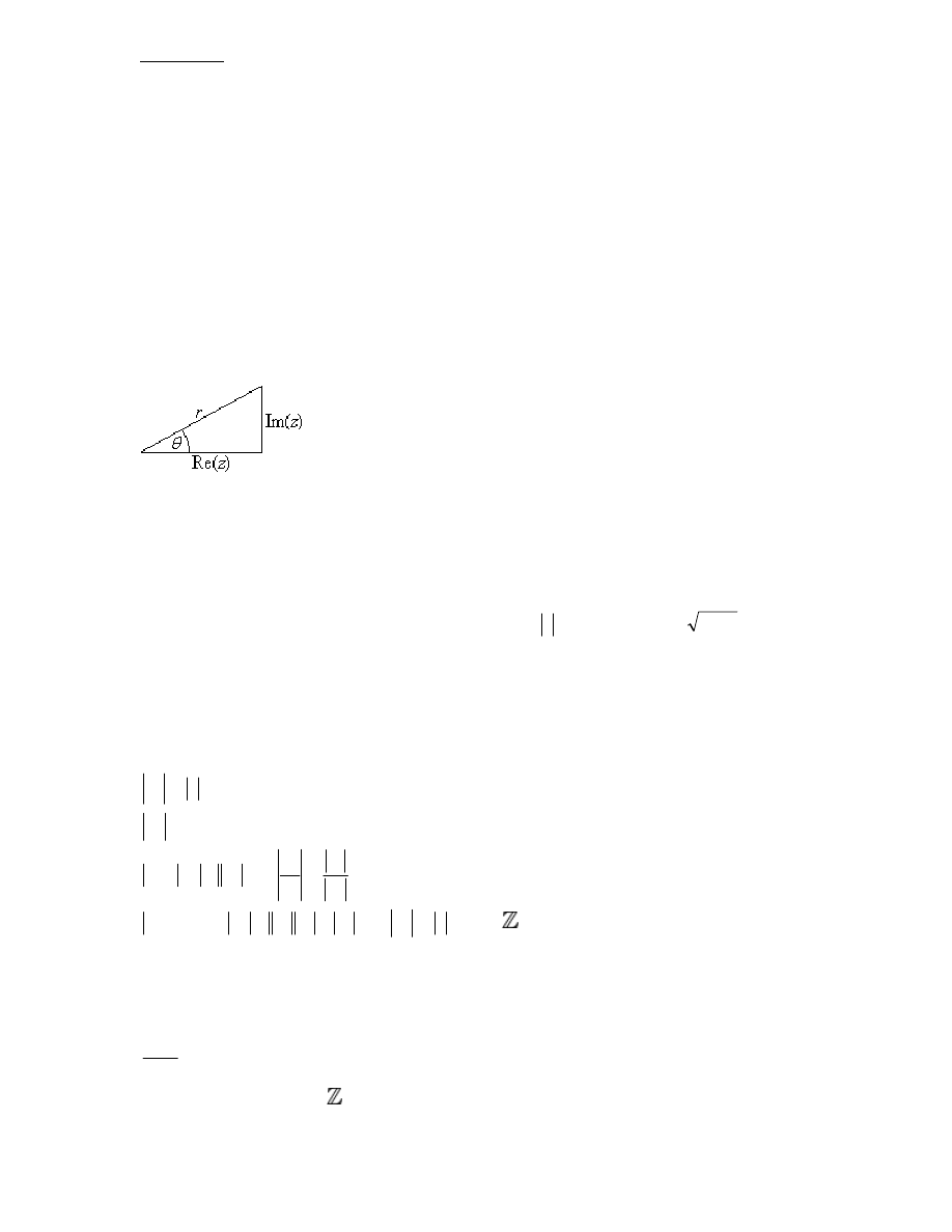
Expressing the complex number on an Argand diagram allows us to express it in terms of
its position relative to the origin: with an argument, or angle θ (in radians) relative to the
x-axis in the positive direction (going anti-clockwise) and a modulus r, or length of the
straight line drawn between the point and the origin. We can thus find the value of the
real part and imaginary part of the complex number in polar form:
As is demonstrated above, the real part can be said to be equal to rcosθ and the
coefficient of the imaginary part can be said to be equal to rsinθ. Thus, the complex
number z can be expressed as
cis
sin
i
cos
sin
i
cos
r
r
r
r
z
. This is
known as the polar, or modulus-argument form.
Note: The modulus r of a complex number is the magnitude of its unit vector on an
Argand diagram. As such, it can also be written as
z
and is equal to
b
a
(from the
complex number as expressed in Cartesian form).
Note: The argument of any complex number z can be expressed as arg z rather than θ.
Notes (all these are easily proven so proofs shall not be made):
0
,
and
2
2
1
2
1
2
1
2
1
2
*
*
z
z
z
z
z
z
z
z
z
zz
z
z
z
n
z
z
z
z
z
z
z
z
z
z
n
n
n
n
,
and
....
....
3
2
1
3
2
1
+
Notes (Proofs may potentially be provided at a later date…):
cis
cis
cis
cis
cis
cis
k
,
cis
k2
cis

Converting between Cartesian and Polar Form
diagram)
Argand
(from
diagram)
Argand
(from
arctan
sin
,
cos
sin
i
cos
i
b
a
r
a
b
r
b
r
a
r
r
b
a
z
Chapter 1.6 – Sums, products and quotients of complex numbers.
Operations with complex numbers are identical to those for radicals.
i
d
c
ad
bc
d
c
bd
ac
d
c
bdi
bci
adi
ac
di
c
di
c
di
c
bi
a
di
c
bi
a
i
bc
ad
bd
ac
bdi
bci
adi
ac
di
c
bi
a
i
d
b
c
a
di
c
bi
a
i
d
b
c
a
di
c
bi
a
2
2
2
2
2
2
2
2
Chapter 1.7 – De Moivre’s theorem. Powers and roots of a complex number.
De Moivre’s theorem states that for any complex number z:
n
r
z
n
n
cis
Notes:
a
b
r
r
z
z
r
r
z
z
n
z
z
r
bi
a
n
arctan
cis
-
cis
arg
arg
cis
2
1
2
1
2
1
2
1
Proof by mathematical induction for De Moivre’s Theorem:
Required to prove that:
n
z
z
n
n
cis
cis
P
1
: If
,
1
n
then
1
1
1
cis
cis
P
z
z
n
is true.
Assume P
k
is true
k
z
z
k
k
cis
cis
P
k+1
:
1
cis
z
cis
z
cis
cis
cis
cis
1
1
k
k
z
k
z
z
z
k
k
k
k
Thus P
k+1
is true whenever P
k
is true and P
1
is true
P
n
is true.

Roots of Complex Numbers
The nth roots of complex number c are the n solutions of z
n
= c.
Two methods of solving: factorisation and the nth root method.
n
th root method:
1
0,1,...,
k
,
2
cis
2
cis
2
cis
1
1
n-
n
k
r
z
k
r
z
k
r
z
c
z
n
n
n
n
Note: the nth roots of unity are the solutions of z
n
= 1
Chapter 1.8 – Conjugate roots of polynomial equations with real coefficients.
Real Polynomials
A real polynomial is a polynomial with only real coefficients:
Polynomials Degree
Name
0
,
a
b
ax
1 Linear
0
,
2
a
c
bx
ax
2 Quadratic
0
,
2
3
a
d
cx
bx
ax
3 Cubic
0
,
2
3
a
d
cx
bx
ax
4 Quartic
0
,
....
1
1
2
3
1
2
1
k
k
x
k
x
k
x
k
x
k
n
n
n
n
n
n
(General)
a, b, c, d, e, k
a or k
1
is the leading coefficient and the term not containing the variable x is the constant
term (as stated above).
Polynomial Multiplication
Every term in the first polynomial must be multiplied by every term in the other.
Algorithm: Synthetic multiplication – detach coefficients and multiply as in ordinary
multiplication of large numbers
Example:
f
ex
d
cx
bx
ax
2
3
a
b
c
d
e
f
af
bf
cf
df
ae
be
ce
de
0
ae
be
af
ce
bf
de
cf
df
4
x
3
x
2
x
1
x
0
x
df
x
de
cf
x
ce
bf
x
be
af
aex
f
ex
d
cx
bx
ax
2
3
4
2
3
Polynomial Division
Division Algorithm: H&H p.170 LEARN (it’s hell to type out on word)
If
x
P
is divided by
b
ax
until a constant remainder R is obtained:
b
ax
R
x
Q
b
ax
x
P
)
(
where
b
ax
is the divisor,
)
(x
P
is the polynomial,
)
(x
Q
is the
quotient and R is the remainder.
Derivations:
R
x
Q
b
ax
x
P
b
ax
R
x
P
x
Q
x
Q
b
ax
x
P
R
x
Q
R
x
P
b
ax
Roots and Zeros
A zero of a polynomial is a value of the variable which makes the polynomial equal to
zero (x-axis intercept). The roots of a polynomial equation are values of the variable
which satisfy the equation in question.
The roots of
0
x
P
are the zeros of
.
x
P
In polynomials of the form:
x
Q
x
x
P
the roots of the equation occur at
0
and the solutions of
x
Q
.
When finding the roots of polynomials, it is important to factorise
x
Q
until it is a
product of linear factors and quadratic factors.
Linear factors of quadratics:
a
ac
b
b
x
a
ac
b
b
x
c
bx
ax
a
ac
b
b
a
ac
b
b
a
ac
b
b
x
x
x
c
bx
ax
2
4
2
4
2
4
2
4
2
4
)
)(
(
0
2
2
2
2
2
2
2
If
,
2
4
2
a
ac
b
b
z
0
*
2
z
x
z
x
c
bx
ax
,
z
z and z
*
are conjugate roots of
0
2
c
bx
ax
For polynomials of even degree, every root has a conjugate root, for polynomials of odd
degree, every root except one has a conjugate root.
Every polynomial of degree
n has n roots, but where there is a factor
0
x
, the
polynomial has repeated roots.

Chapter 2.1 – Concept of function
:
( )
f x
f x
: domain, range; image (value).
Composite functions
;
f g
identity function. Inverse function
1
f
.
Algebraic Test: If a relation is given as an equation, and the substitution of any value for
x results in one and only one value of y, we have a function. (Note that the algebraic test
can be used as a definition for what a function is).
Geometric Test: If at any point along the
x-axis, there are two y-axis values, the graph is
not a function.
In composite functions, the right-most function is a function of
x and those that aren’t are
merely functions of the functions the right of it. That is to say that if you define a
function
f x
as a relationship given as an equation where the substitution of any value
for
x results in one and only one value of y, the definition of the function
:
g f x
g f x
is a relationship given as an equation where the substitution for any
value for
f x
results in one and only one value of
y.
The domain of a relation is the set of permissible values that
x may have.
The range of a relation is the set of permissible values that
y may have.
Note: The stated domain and range of the relation in question must be applied before it is
determined whether or not this relation constitutes a function.
Interval Notation
:
,
:
,
:
,
:
,
:
:
: 2
,
: 2
,
x a
x x a
x
a
y a
y y a
y
a
x a
x x a
x
a
y a
y y a
y
a
x x
x
y y
y
a x b
x
x b
x
a b
a y b
y
y b
y
a b
[
a means that a is the lower limit and that x can equal a
]
a means that a is the upper limit and that x can’t equal a
b] means that b is the upper limit and that x can equal b
b[ means that b is the upper limit and that x can’t equal b.
]
, [
where there is no limit on one side, must be excluded in the notation.

Inverse functions
Where a function
f x
substitutes
x values for a different value, the inverse function
1
f
x
is the function that substitutes
f x
values for
x values. Graphically, the inverse
of a function is that function reflected in the line
y x
.
As a direct result of this, any function in which more than one
x value is substituted to the
same value of
y (called a many-to-one function) has no inverse. This is represented
graphically by the horizontal bar test, where if you can draw a line parallel to the
x-axis
that crosses the function more than once, the function has no inverse (if the converse is
true, then the function is a one-to-one function). Otherwise stated, one-to-one functions
have an inverse whereas many-to-one functions do not. The domain must be taken into
account when categorising a function as one-to-one rather than many-to-one, for example
sin
f x
x
appears to be a many-to-one function, but if the domain is 0,
2
then the
function is a one-to-one function and has an inverse.
Chapter 2.2 – The graph of a function; its equation
y
f x
. Function graphing skills:
use of a GDC to graph a variety of functions, investigation of key features of graphs,
solutions of equations graphically.
When functions are graphed, the function
f x
is always represented on the
y axis.
The asymptote is an
x or y value for which there is defined value of the function,
generally appearing where the denominator in the function has gone to 0.
The roots or equations (or zeros of functions) can be found graphically by noting the
points at which the function crosses the
x axis. For the solution to two equations
represented as functions as
f x
and
g x
respectively where
f x
g x
, the
solution(s) can be found at the intercept(s) of the two functions.
Chapter 2.3 – Transformations of graphs: translations; stretches; reflections in the axes.
The graph of
1
y
f
x
as the reflection in the line
y x
of the graph of
y
f x
.
The graph of
1
y
f x
from
y
f x
. The graphs of the absolute value functions,
y
f x
and
y
f x
.
Transformations:
y
f x
b
translates the graph
b units in the positive y direction.
y
f x a
translates the graph
a units in the positive x direction.
( )
y
pf x
stretches the graph parallel to the
y-axis with factor p.
x
y
f
q
stretches the graph parallel to the
x-axis with factor q.

y
f x
reflects the graph in the
x-axis.
y
f
x
reflects the graph in the
y-axis.
If given
f x
and required to graph
1
f x
, realise where the graph of ( )
f x gets
steeper, the graph of
1
f x
gets flatter, and that the greater the magnitude of
f x
at
any point
x, the magnitude of
f x
is lesser. However, where ( )
f x is less than 1 and
tends towards 0, the slope gets steeper until it reaches the asymptote at ( ) 0
f x
.
( )
y
f x
The domain where ( ) 0
f x
is reflected in the x-axis, all else is unchanged.
y
f x
The domain
0
x
is taken and the graph is reflected in the
y-axis.
Properties of
R
x
x
,
x
is the distance from 0 to
x on the number line
2
2
2
x
x
x
x
0
x
x
x
x
x
y
x
y
x
y
x
xy
Z
n
x
x
n
n
,
y
x
y
x
y
x
y
x
a
x
is the difference between
x and a on the real number line
x
y
y
x
Chapter 2.4 – The reciprocal function
1
,
x
x
0
x
: its self-inverse nature.
Since the function that maps
1
x
onto
x is known as the inverse of
1
,
x
x
0
x
and is
1
x
, the reciprocal function is effectively its own inverse.
Chapter 2.5 – The quadratic function
2
x
ax
bx c
: its graph. Axis of symmetry
2
b
x
a
. The form
2
x
a x h
k
. The form
.
x
a x p x q
All quadratic functions can be written in the form
2
x
ax
bx c
. However, some can
be written in the form
,
x
a x p x q
0
a
while others can also be written in the

form.
2
x
a x h
k
. If
0
k
, the quadratic can only be written in the latter form
(short of using complex roots) however if
0
k
, the quadratic can be expressed in both
forms.
The first form is beneficial for finding the roots of the quadratic, since they are equal to
p
and
q. The second, however, is much more useful for finding the axis of symmetry (h) of
the quadratic and determining where the minimum (or maximum for
0
a
) point (
k) of
the quadratic is.
Thanks to the properties of the second equation, putting the general equation for
2
x
ax
bx c
in the form
2
x
a x h
k
allows us to find the general equation for
the position of the axis of symmetry and the position of the min/max point on the graph.
Completing the square:
2
2
2
2
2
2
2
2
2
2
2
2
2
2
2
2
2
2
2
4
2
4
,
2
4
2
bx
ax
bx c a x
c
a
b
b
b
a x
x
c
a
a
a
b
b
b
a x
x
c
a
a
a
b
b
a x
c a x h
k
a
a
b
b
h
c k
a
a
b
h
a
Chapter 2.6 –The solution of
2
0,
ax
bx c
0
a
. The quadratic formula. Use of the
discriminant
2
4
b
ac
.
Completing the square also allows us to find the general equation for the roots of an
equation.

2
2
2
2
2
2
2
2
2
2
2
2
2
2
2
2
0
2
4
0
2
4
4
2
4
4
2
4
4
4
2
4
2
4
2
2
4
2
ax
bx c
b
b
ax
bx c a x
c
a
a
b
b
a x
c
a
a
b
b
ac
a x
a
a
b
b
ac
x
a
a
b
b
ac
b
ac
x
a
a
a
b
b
ac
x
a
a
b
b
ac
x
a
This equation is known as the quadratic formula.
What is important to note in this formula is the discriminant
2
4
b
ac
. This
determines whether or not the quadratic has a real solution.
Where
0
, the quadratic has two repeated roots, where
0
, the quadratic has two
different roots and where
0
the quadratic has no real roots.
Chapter 2.7 – The function:
x
x
a
,
0
a
. The inverse function
log ,
a
x
x
0
x
.
Graphs of
x
y a
and
log
a
y
x
. Solutions of
x
a
b
using logarithms.
The function
x
x
a
has a curvature that tends towards zero as x tends towards infinity.
The curvature also tends towards zero as x tends towards negative infinity. The gradient,
however, constantly increases from 0 at
x
to
1
0
at
x
. Its inverse function is
merely a reflection of this in the x-axis.
We can find the solutions of
x
a
b
using logarithms:
log
log
log
x
x
a
a
a
a
b
a
b
x
b
For harder equations, the solutions can be found the following way:

log
log
log
log
x
x
a
b
a
b
b
x
a
Chapter 2.8 – The exponential function
x
x
e
. The logarithmic function
ln
x
x
,
0
x
.
It is known from topic 1.1 that the equation for compound interest is:
n
n
r
u
u
1
1
, where
1
u
initial investment,
%
100
%
%
100
i
r
,
i interest rate per
compounding period, n = number of periods and
1
n
u
amount after n periods.
It is clear that
i
r
1
, and that if we treat the initial investment to be the 0
th
term, we get
an equation where
n
n
n
i
u
r
u
u
1
0
0
.
If r is (instead) the percentage rate per year, t the number of years and N the number of
interest payments per year, then
rt
r
N
Nt
n
r
N
u
N
r
u
u
1
1
1
0
0
Let
a
r
N , then
rt
a
rt
a
n
a
u
a
u
u
1
1
1
1
0
0
But
a
x
x
e
a
ln
where a and x are any real number, thus:
rt
a
n
a
u
u
1
1
0
1
lim 1
e
a
a
a
0
rt
n
u
u e
for large values of a.
Growth and decay works in a similar way, putting the sequence in the form
0
1
1
a
n
u
u f
a
.
Chapter 2.9 – Inequalities in one variable, using their graphical representation. Solution
of ( )
( )
g x
f x
, where ,
f g are linear or quadratic.
Inequalities can be solved using a sign diagram, where it is key to remember that the
arrow represents all the values for which
0
)
(
x
f
, regardless of whether we’re trying to
find the values for which the overall function is greater than or less than x.

Inequality laws:
c
b
c
a
b
a
,
b
a
0
c
bc
ac
and
c
b
c
a .
,
b
a
0
c
bc
ac
and
c
b
c
a .
.
0
2
2
b
a
b
a
Sign Diagram Notes:
The horizontal line of a sign diagram corresponds to the x-axis.
The critical values are values of x when the function is zero or undefined.
A positive sign (+) corresponds to the fact that the graph is above the x-axis.
A negative sign (
) corresponds to the fact that the graph is below the x-axis.
When a factor has an odd power there is a change of sign about that critical value. When
a factor has an even power there is no sign change about that critical value.
For a quadratic factor
c
bx
ax
2
where
;
0
4
2
ac
b
.
0
,
,
0
,
0
,
,
0
2
2
a
R
x
c
bx
ax
a
R
x
c
bx
ax
There is no critical value in either case.
Solving inequalities: Procedure
Make the RHS = 0 by transferring all terms to LHS.
Fully factorise the LHS.
Draw a sign diagram of the LHS.
Solve.
Note: Do not, under any circumstances, cross-multiply. This removes certain terms from
the equations and prevents one from finding all the solutions.
Chapter 2.10 – Polynomial functions. The factor and remainder theorems, with
application to the solution of polynomial equations and inequalities.
It is important to note that the higher the order of the polynomial function, the steeper the
line for
1
x
and the less steep the line for
1
x
. Odd orders have negative values
where x < 0 but even order always having positive values unless translated down.
Repeated roots merge on a graph to appear as only one root. Repeated roots signify a
point of inflection.
The factor theorem
According to polynomial division,
R
k
x
x
Q
x
P
)
(
)
(
Thus, where x = k
R
k
P
R
k
Q
k
P
)
(
0
)
(
)
(

Therefore when polynomial
)
(
x
P
is divided by
k
x
until a constant remainder R is
obtained then
)
(
k
P
R
The remainder theorem
If k is a zero of P(x) thus:
k
x
x
x
P
R
k
P
x
P
)
(
)
(
0
0
)
(
)
(
k
x
is a factor of P(x)
In general:
).
(
of
factor
a
is
)
(
of
zero
a
is
x
P
k
x
x
P
k
Using the remainder theorem to find the remainder allows us to find how far the
minimum/maximum point of the graph of
0
)
(
)
(
R
x
Q
x
P
is shifted away from the x-axis.
Using the factor theorem allows us to quickly find the roots (if the factor is known) or the
factors (if the root is known) of the polynomial equation and thus solve polynomial
equations and inequalities quickly.
Chapter 3.1 – The circle: radian measure of angles; length of an arc; area of a sector.
One radian is defined as the angle that subtends an arc of length equal to the radius. Thus,
2
1
2
2
arc
total
arc
total
r
C
C
r
r
r
Thus 1 radian is
1
2
of the angle of a full circle, thus there are
2
radians per full turn.
This means that: 2
360
c
, so
180
1
c
and 1
180
c
.
Thus, the length of an arc in radians is:
2
2
l
r
r
And the area of a sector is:
2
2
2
2
r
A
r
Chapter 3.2 – Definition of
cos
and
sin
in terms of the unit circle. Definition of
tan
as
sin
cos
. Definition of sec ,
csc
and
cot .
Pythagorean identities:
2
2
cos
sin
1;
2
2
1 tan
sec ;
2
2
1 cot
csc .
The Sine Function
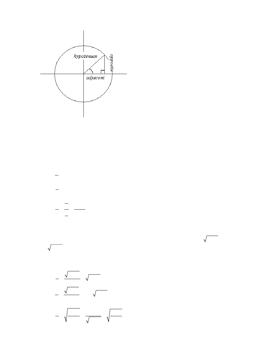
The sine function of
means that for a right angled triangle with angle (as shown in
the diagram), the ratio of the length of the opposite side to that of the hypotenuse is equal
to the sine function of
.
Pythagoras’s theorem states that
2
2
2
a
b
c
where a is the opposite side, b is the
adjacent side and c is the hypotenuse, thus we can state that:
sin
cos
sin
tan
cos
a
c
b
c
a
a
c
b
b
c
The unit circle has radius 1. This means that the hypotenuse has radius 1. We can thus
use Pythagoras’s Theorem to state that
2
2
1
a
b
and that therefore
2
1
a
b
and
2
1
b
a
.
Thus, in terms of the unit circle,
2
2
2
2
1
cos
1
1
1
sin
1
1
b
a
a
b
c
a
b
a
b
c
And
2
2
2
2
1
tan
1
1
1
a
b
a
b
b
a
b
a

This tells us the variance of each function in terms of the unit length of the opposite and
in terms of the unit length of the adjacent. In the plotting the sine curve, we plot a on the
y-axis and
on the x-axis.
Thus we obtain:
2
2
2
2
2
2
2
2
sin
1
cos
1
cos
1 cos
sin
sin
cos
1
a
a
a
a
And
2
2
2
2
2
2
2
2
2
2
2
2
2
2
2
2
2
2
tan
1
tan
1
sin
sin
tan
1 sin
1 sin
sin
sin
1 tan
1
1 sin
1 sin
1 sin
cos
1
1 tan
sec
cos
a
a
a
a
a
Also
2
2
2
2
2
2
2
2
2
2
2
2
2
sin
tan
1 sin
1
1 sin
cot
tan
sin
sin
1 sin
1
1 cot
csc
sin
sin
Chapter 3.3 – Compound angle identities. Double angle identities.
Compound angle identities
Equation booklet:
sin(
) sin cos
cos sin
A B
A
B
A
B

Proof
Consider P(cos , sin )
A
A and Q(cos , sin )
B
B as any two points on the unit circle.
Angle POQ is A B
Using the distance formula:
2
2
2
2
2
2
2
2
2
2
2
PQ
cos
cos
sin
sin
PQ
cos
2cos cos
cos
sin
2sin sin
sin
cos
sin
cos
sin
2 cos cos
sin sin
1 1 2 cos cos
sin sin
2 2 cos cos
sin sin
A
B
A
B
A
A
B
B
A
A
B
B
A
A
B
B
A
B
A
B
A
B
A
B
A
B
A
B
But according to the cosine rule,
2
2
2
PQ
1
1
2 1 1 cos
2 2cos
A B
A B
cos
cos cos
sin sin
A B
A
B
A
B
If we state that
cos
cos cos
sin cos
, we can let
B
and
A
.
cos
cos cos
sin cos
can also be written as:
cos
cos cos
sin sin
cos
cos cos
sin sin
sin
sin
cos
cos
cos
cos cos
sin sin
A B
A
B
A
B
B
B
B
B
A B
A
B
A
B
sin
cos
2
cos
2
cos
cos
sin
sin
2
2
sin cos
cos sin
A B
A B
A
B
A
B
A
B
A
B
A
B
It is also clear that
sin
sin cos
cos sin
A B
A
B
A
B
tan
tan
tan
1 tan tan
A
B
A B
A
B
Double angle identities
sin 2
sin
sin cos
cos sin
2sin cos
A
A A
A
A
A
A
A
A
2
2
sin 2
sin
cos cos
sin sin
cos
sin
A
A A
A
A
A
A
A
A
2
2
2
2
2
2
2
2
2
2
cos 2
cos
sin
cos
cos
1
2cos
1
cos 2
cos
sin
1 sin
sin
1 2sin
A
A
A
A
A
A
A
A
A
A
A
A
2
tan
tan
2 tan
tan 2
1 tan tan
1 tan
A
A
A
A
A
A
A
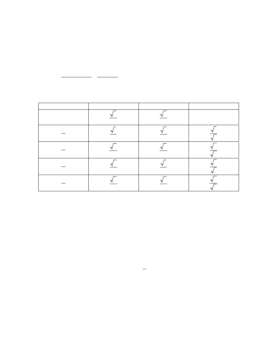
Trig identities table:
Angle Sine Cosine
Tangent
0
0
2
4
2
0
6
1
2
3
2
1
3
4
2
2
2
2
2
2
3
3
2
1
2
3
1
2
4
2
0
2
4
0
Chapter 3.4 – The circular functions
sin
x
,
cos
x
and tan x ; their domains and ranges;
their periodic nature; their graphs. Composite functions of the form
sin
f x
a
b x c
d
. The inverse functions
arcsin
x
x
, arccos
x
x
,
arctan
x
x
; their domains and ranges; their graphs.
The period of the untranslated sine and cosine functions is
2
and their range is 1.
In the form
sin
f x
a
b x c
d
,
a represents a stretch from the x-axis of factor a,
b represents a stretch from the y-axis of factor
1
b
,
c represents a translation c units to the left
d represents a translation d units upward.
The reciprocal functions can be derived through common sense.
The inverse function can only be derived by restricting the domain to
for all the
trigonometric functions, then reflecting in the line y x
.
Chapter 3.5 – Solutions of trigonometric equations in a finite interval. Use of
trigonometric identities and factorisation to transform equations.
For the first one: Use the inverse functions, then add or subtract
2
(or ) accordingly.
For the second one: Use trigonometric identities to find alternative ways of writing
certain transformations. In short, put trigonometric functions into the form
sin
f x
a
b x c
d
using factors and identities to be able to describe the
transformation.
Chapter 3.6 – Solution of triangles. The cosine rule:
2
2
2
2
cos
c
a
b
ab
C
. The sine
rule:
sin
sin
sin
a
b
c
A
B
C
. Area of a triangle as
1
sin
2
ab
C .
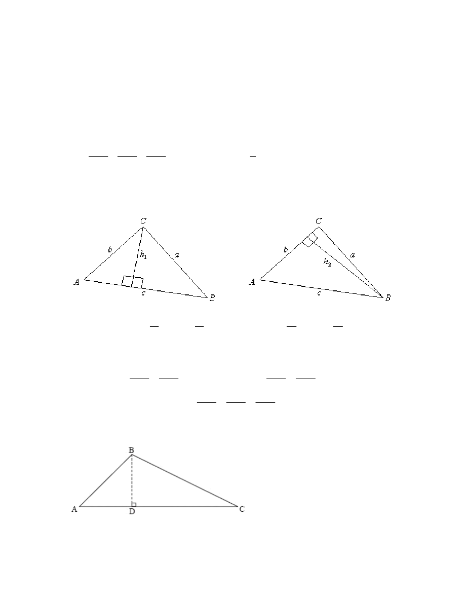
Any triangle with vertices A, B, C and sides a, b, c can be made into two right-angled
triangles as shown.
B
b
A
a
B
a
A
b
B
a
h
A
b
a
h
B
b
h
A
sin
sin
sin
sin
sin
sin
sin
,
sin
1
1
1
C
c
A
a
C
a
A
c
C
a
h
A
c
a
h
C
c
h
A
sin
sin
sin
sin
sin
sin
sin
,
sin
2
2
2
C
c
B
b
A
a
sin
sin
sin
The cosine rule can be proved as follows using the triangle below.
CD AC AD
cos
b c
A

2
2
2
2
2
2
2
2
2
2
2
2
2
2
2
2
2
2
2
BC
BD
CD
sin
cos
sin
2 cos
cos
sin
cos
2 cos
1
2 cos
2 cos
a
c
A
b c
A
c
A b
bc
A c
A
b
c
A
A
bc
A b
c
bc
A
b
c
bc
A
Chapter 4.1 – Definition of a matrix: the terms element, row, column and order.
A matrix is a rectangular array of numbers arranged in rows and columns.
A row is a horizontal set of numbers.
A column is vertical set of numbers.
The order of a matrix denotes the number of rows and number of columns in the matrix
and is equal to the number of elements in the matrix:
m n
where m is the number of
rows and n is the number of columns.
Chapter 4.2 – Algebra of matrices: equality; addition; subtraction; multiplication by a
scalar. Multiplication of matrices. Identity and zero matrices.
Two matrices are equal if they are of the same order.
It is only possible to add or subtract two matrices if they are of the same order. Each
element of a particular row and column is added or subtracted by the corresponding
element in the other matrix.
Multiplication by a scalar involves the mere multiplication of every term in the matrix by
that scalar.
Two matrices can only be multiplied together if the first (matrix multiplication is not
commutative) matrix has the same number of columns as the second has rows. The
resulting matrix has the same number of rows of the first matrix and the same number of
columns as the second.
p
a b c q
ap bq cr
r
.
The identity matrix I is the matrix such that A
I = A where A is any square matrix. For
2 2
matrices,
1 0
I
0 1
and for
3 3
matrices,
1 0 0
I
0 1 0
0 0 1
To prove this,
Let A
a b
c d
AI = A (by definition). Let
p q
I
r
s
Thus:

2
2
2
2
0
1
1
0
1
1
1
0
1
a b
p q
a b
c d
r
s
c d
ap br
aq bs
a b
cp dr
cq ds
c d
ap br a
aq bs b
cp dr c
cq ds d
ap br a
ap a br
a br
a
p
a br
ap br
p
ap
brp a br
ap
a brp br
a p
br p
a p
p
br p
p
a p
1
0
1
1
0
0
1 0
0 1
br
p
s
r
q
p q
r
s
A zero matrix is a matrix in which all elements are equal to 0 such that
AO = O and A + O = A
It is important to note that multiplication by both the identity and the zero matrix is
commutative.

Here are some rules:
If A and B are matrices that can be multiplied then AB is also a matrix.
Matrix multiplication is non-commutative.
If O is a zero matrix then AO = OA = O for all A.
A(B + C) = AB + AC
If I is the identity matrix then AI = IA = A
A
n
for n
2 can be determined provided that A is a square and n is an integer.
Chapter 4.3 – Determinant of a square matrix. Calculation of
2 2
and
3 3
determinants. Inverse of a matrix: conditions for its existence.
The inverse of a matrix A
-1
is such as will satisfy the equation AA
-1
= A
-1
A = I.
1 0
0 1
1 0
0 1
1
0
0
1
1
0
1
0
1
1
1
a b
p q
c d
r
s
ap br aq bs
cp dr cq ds
ap br
aq bs
cp dr
cq ds
ap br
cp dr
ap br
ad
ap
r
c
ad
b
r
c
c
c
r
bc ad
ad bc
bc
ad
ad
ap
br
bc ad
bc ad
ad bc
ad
p
d
ad bc a
ad bc
a
s
ad bc
bc
b
q
ad bc c
ad bc

1
d
b
p q
d
b
ad bc
ad bc
r
s
c
a
c
a
ad bc
ad bc
ad bc
This suggests that there is no inverse for any matrix where
0
ad bc
. A matrix without
an inverse is known as a singular matrix, and
ad bc
is known as the determinant
because it determines whether the matrix will be singular or invertible.
The determinant of matrix A is written as
A
and as
det A
.
Rules: detAB = detAdetB.
The determinant of a
3 3
matrix:
Where A =
1
1
1
2
2
2
3
3
3
a
b
c
a
b
c
a
b
c
,
2
2
2
2
2
2
1
1
1
3
3
3
3
3
3
A
b
c
c
a
a
b
a
b
c
b
c
c
a
a
b
.
Chapter 4.4 – Solutions of systems of linear equations (a maximum of three equations in
three unknowns). Conditions for the existence of a unique solution, no solution and an
infinity of solutions.
-1
AX B
X A B
Above is how to solve simultaneous equations.
Row Operations (simultaneous equations):
The equations can be interchanged without affecting the solutions
An equation can be replaced by a non-zero multiple of itself
Any equation can be replaced by a multiple of itself
a multiple of another equation.
Augmented Matrix Form
ax by c
px qy r
can be written as
a b c
p q
r
`
We can now manipulate the equations using row operations to get a matrix in the form
0
a b c
p
q
From which we may get a unique solution.
If a matrix
a b c
a b
d
is obtained, the equation has no solution.

If a matrix
2
2
2
a b c
a
b
c
is obtained then there are infinitely many solutions.
Reduced row echelon form allows us to find unique solutions to simultaneous equations:
1
1
1
1
2
2
2
2
3
3
3
3
0
0 0
a
b
c
d
a b c
d
a
b
c
d
e
f
g
a
b
c
d
h
i
If
0
h
we arrive at a unique solution.
If
0
h
and
0
i
, there is no solution and the system is inconsistent.
If
0
h
and
0
i
, there are infinitely many solutions of the form x
p kt
, y q lt
and
,
z t
t
An underspecified system (not enough equations) is the same case as the last one above.
The system may have no solutions, as may be seen by looking for inconsistencies.
If a simultaneous equation in augmented matrix form is invertible, it has a unique
solution. If it is singular, it has either no solutions or infinitely many. Converting the
augmented matrix to reduced row echelon form allows us to determine which.
Chapter 5.1 – Vectors as displacements in the plane and in three dimensions.
Components of a vector; column representation
1
2
1
2
3
3
v
v
v
v i v j v k
v
. Algebraic and
geometric approaches to the following topics: the sum and difference of two vectors; the
zero vector, the vector
v
; multiplication by a scalar,
kv
; magnitude of a vector, v
; unit
vectors , , ;
i j k
position vectors
a
OA
.
A vector
1
2
1
2
3
3
v
v
v
v i v j v k
v
represents a translation of
1
v units along the x-axis,
2
v units along the y-axis and
3
v units along the z-axis. This is because , , and
i j
k
are unit
vectors (vectors with a magnitude of 1) where
1
0
0
i
,
0
1
0
j
and
0
0
1
k
and thus
represent translations in each of the three axes.
The distance between any two points in three (or two) dimensions is given (by definition)
by the magnitude of the vector that maps one of the points onto the other. This is given in
the equation
2
2
2
1
2
3
v
v
v
v
.
For two general points
1
1
1
A( , , )
x y z and
2
2
2
B( , , )
x y z in a three dimensional space,
2
2
2
2
1
2
1
2
1
AB
(
)
(
)
(
)
x
x
y
y
z
z

The zero vector is a vector
0
0
0
such that
0
0
a a a
.
If
v
maps point A onto point B, then
v
maps point B onto point A.
Summary of vector arithmetic
1
1
2
2
3
3
1
1
2
2
3
3
if , ,
a
b
a
a
b
b
a
b
a
b
a b
a
b
a
b
(
)
(
)
0 0
(
)
0
a b b a
a b
c a
b c
a
a a
a
a
a
a
Also, ka
k a
1
x a b
x b a
k x a
x
a
k
if OA
and OB
, then AB
, BA
a
b
b a
a b
(
OA
is a position vector, mapping the origin onto a point A).
Definitions
Two vectors are equal if they have the same magnitude and direction, but do not have to
be on the same line:
and
p
r
p r
q s
q
s
Points are collinear if they lie on the same line:
A, B and C are collinear if AB
BC for some scalar .
k
k
is parallel to
for some scalar .
a
b
a kb
k
1
v
v
is the length of the unit vector in the direction of
v
.

Chapter 5.2 – The scalar product of two vectors,
cos
v w
v w
;
1 1
2
2
3
3
v w v w
v w
v w
. Algebraic properties of the scalar product. Perpendicular
vectors. The angle between two vectors.
The scalar product of two vectors, also known as the dot product or inner product of two
vectors,
v w
gives us a scalar answer. The scalar product is defined by the second
equation,
1 1
2
2
3
3
v w v w
v w
v w
, but it can be proved that the first equation is also true,
cos
v w
v w
using the method described on p.381, H&H.
A consequence of
cos
v w
v w
is that for parallel vectors, where
0
, the
equation gives
cos 0
v w
v w
v w
and for perpendicular vectors, where
2
, the
equation gives
cos
0
2
v w
v w
. Thus, it is possible to find the solution for missing
variables by setting
2
2
2
2
2
2
1 1
2
2
3 3
1
2
3
1
2
3
v w
v w
v w
v
v
v
w
w
w
and by setting
1 1
2
2
3
3
0.
v w
v w
v w
Algebraic properties of the scalar product
2
a b b a
a a
a
a
b c
a b a c
a b
c d
a c a d b c b d
Chapter 5.3 – Vector equation of a line
r a
b
. The angle between two lines.
In 3-D:
0
0
0
x
x
l
y
y
m
z
z
n
is the vector equation of a lie where
, ,
R x y z
is any point on the
line and
0
0
0
, ,
A x y z
is any point on the line.
l
b
m
n
is the direction vector of the line
(see collinear points). Thus,
0
0
0
x
y
z
maps one point in three-dimensional space from the
origin and
l
m
n
tells us the general position of all collinear points.
The parametric equations of the line, describing the line as a two-dimensional line on the
.
x, y and z planes respectively, are used when writing the lines in parametric form:
0
0
0
, , ,
x x
l y
y
m z z
n
.
Cartesian form, setting each equation equal to
and thus equal to one another, gives us
the following:
0
0
0
x x
y y
z z
l
m
n
.
The angle between the two lines in three dimensional space can be found using the scalar
product of their direction vectors:
1 2
1
2
1 2
2
2
2
2
2
2
1
1
1
2
2
2
arccos
l l
m m
n n
l
m
n
l
m
n
(values taken from the equations of the lines).
Chapter 5.4 – Coincident, parallel and skew lines, distinguishing between these cases.
Points of intersection.
Two lines are coincident if the Cartesian equations of one are a scalar multiple of the
other.
Two lines are parallel if the angle between the two lines found using the scalar product of
their direction vectors is 0 angular units, but the Cartesian equations of one is not a scalar
multiple of the others.
Two lines are intersecting if the angle between the two lines found using the scalar
product of their direction vectors is
θ angular units and they intersect at a point found by
representing their equations as matrices and solving them (see chapter 4.4).
Two lines are skew if the angle between the two lines found using the scalar product of
their direction vectors is
θ angular units and representing their equations as matrices
gives no solution (see chapter 4.4).
Another way of finding points of intersection is as follows.
Take two lines
1
2
and
L
L where:
1
0
1
0
1
0
1
2
1
2
2
2
3
2
: , ,
: , ,
L x x
l y
y
m z z
n
L
x a
l y a
m z a
n
If:
1
0
2
0
3
0
1
2
1
2
1
2
a
x
a
y
a
z
l
l
m
m
n
n
, the lines intersect at coordinates found by substituting
the obtained value of
into the parametric equations.

Chapter 5.5 – The vector product of two vectors,
v w
. The determinant representation.
Geometric interpretation of
v w
.
The vector, or cross product of two vectors,
v w
is a function of the two vectors which
gives a vector perpendicular to the two vectors. Thus, the vector product of two vectors
v
and
w
where
1
2
3
v
v
v
v
and
1
2
3
w
w
w
w
is given by:
2
3
3 2
2
3
3
1
1
2
3 1
1 3
1
2
3
2
3
3
1
1
2
1 2
2 1
1
2
3
v w
a b
i
j
k
v
v
v
v
v
v
v w
v w v w
v
v
v
i
j
k
w
w
w
w
w
w
v w
v w
w
w
w
.
1
2
3
1
2
3
i
j
k
v
v
v
w
w
w
is known as a
3 3
determinant.
A normal is a line perpendicular to a plane. Thus, given two vectors (or three points) on a
plane, a normal to the plane can be found. Since it’s a direction vector, any scalar
multiple of a normal vector in its simplest form is usable.
Vector product algebra
1
2
3
1
2
3
1
2
3
,
0
and is called the scalar triple product.
v w v w
v v
v w
w v
a
a
a
a
b c
b
b
b
c
c
c
a
b c
a b
a c
a b
c d
a c
a d
b c
b d
2
2
2
2
3
3
2
3 1
1 3
1 2
2 1
sin , .
v w
v w
v w
v w v w
v w
v w
v w
v w
Properties
1
If ,
sin
0
.
u
v w
v w
v w
u
v w
v w
v w
1
If a triangle has defining vectors and then its area is
.
2
v
w
v w

Thus, if a parallelogram has defining vectors and then its area is
.
v
w
v w
Chapter 5.6 – Vector equation of a plane r
a
b
c
. Use of normal vector to obtain
the form
r n a n
. Cartesian equation of a plane
ax by cz d
.
Since a plane in three dimensional space can be described using a minimum of two lines
on the plane, and the vector equation of one line in space is given by
r a
b
where
a
is a vector mapping the origin onto one point on the line and
b
is a the direction vector of
the line, the vector equation of the plane can be found by adding the direction vector of
another line to the equation, i.e.
r a
b
c
where
b
and
c
are two non-parallel
vectors that are parallel to the plane.
If A is a point on a plane and R is another point on the plane, then
AR OR OB r a
where
r
is the position vector of R (which is a general point ( , , )
x y z on the plane) and
a
is the position vector of A. Thus, the normal to the plane will also be perpendicular to
that line, so:
0
0
n
r a
n r n
a
n r
n
a
n r n a
This is a different way of expressing the vector equation of a line. This means that if a
normal vector
a
b
c
passes through a point
0
0
0
( , , )
x y z then:
ax by cz d
, where d is some constant. This gives us the Cartesian equation of the
line:
0
0
0
ax
by
cz
ax by cz d
where
a
b
c
is a normal vector of the plane.
Chapter 5.7 – Intersections of: a line with a plane; two planes; three planes. Angle
between: a line and a plane; two planes.
When given the Cartesian equation of a plane, the intersection of a line with the plane can
be found by using the parametric form for expressing the line in terms , , and
x y z
and
substituting each into the Cartesian equation of the plane, thus solving for
(as shown in
H&H, p. 446 example 20).
Take two planes
1
2
and
P
P where:
1
0
1
1
0
1
1
0
1
1
2
1
2
2
2
2
2
3
2
2
: , ,
: , ,
P x x
l
d y
y
m
e z z
n
f
P x a
l
d y a
m
e z a
n
f

Thus, the line of intersection of a plane can be found by setting the equations of either
x,
y or z equal to one another and solving for in terms of
or in terms of
and thus
substituting it into the two remaining equations to solve for the remaining constant. The
two values found, substituting them into the parametric form equations gives the
coordinates of a point of intersection. This method is extremely long and inefficient,
however. Keeping the equations in terms of
will yield a line described in parametric
form, however.
The intersection of three planes is found by using the Cartesian forms of the three vectors
and inputting them into an augmented matrix to solve for
x, y and z. If no solutions are
yielded, there is no common point of intersection. If a unique solution is yielded, the
three planes meet at a point. If there is are an infinite number of solutions, the planes
meet at a line with parametric equations given by the matrix where
z is substituted by a
variable
t.
Alternatively, if the three planes meet at a point, the inverse matrix method mentioned
earlier can be used:
-1
AX B
X A B
Finding whether or not the determinant of A exists can be a quick method for
determining whether or not the three planes meet at a point.
The angle between a line with direction vector
d
and a plane with normal vector
n
is
found using the equation
arcsin
n d
n d
(see H&H p.449).
If two planes have normal vectors
1
n
and
2
n
, the acute angle
between the two
intersecting planes is given by
1
2
1
2
arccos
n n
n n
. The obtuse angle
180
.
Chapter 6.1 – Concepts of population, sample, random sample and frequency
distribution of discrete and continuous data.
A population is the set of all individuals with a given value for a variable associated with
them.
A sample is a small group of individuals randomly selected (in the case of a random
sample) from the population as a whole, used as a representation of the population as a
whole.
The frequency distribution of data is the number of individuals within a sample or
population for each value of the associated variable in discrete data, or for each range of
values for the associated variable in continuous data.
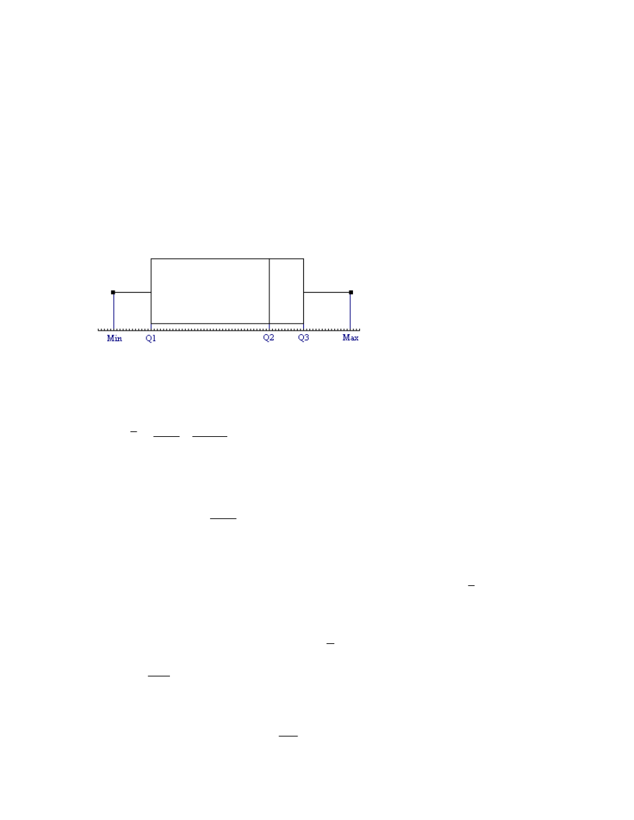
Chapter 6.2 – Presentation of data: frequency tables and diagrams, box and whisker
plots. Grouped data: mid-interval values, interval width, upper and lower interval
boundaries, frequency histograms.
Mid interval values are found by halving the difference between the upper and lower
interval boundaries. The interval width is simply the distance between the upper and
lower interval boundaries. Frequency histograms are drawn with interval width
proportional to bar width and frequency as the height.
Box and whisker plots
A box-and-whisker plot is a visual display of some of the descriptive statistics of a data
set. It show The minimum value (Min
x
), the lower quartile (Q
1
), the median (Q
2
), the
upper quartile (Q
3
) and the maximum value (Max
x
). These quantities are known as the
five-number summary of a data set.
Chapter 6.3 – Mean, median, mode; quartiles, percentiles. Range; interquartile range;
variance, standard deviation.
Mean:
1
1
1
n
n
i
i i
i
i
n
n
i
i
x
f x
x
n
f
Median:
1
where
2
n
i
i
m
m
f
x x
f
Mode: Mode
where
,
r
r
i
x
f
f i r
The population mean, ,
is generally unknown but the sample mean,
x serves as an
unbiased estimate of this mean.
A quartile (Q
s
) is a the value of
i
x which has
4
s
of the total frequency falling below this
value and
1
4
s
of the total frequency falling above this value. This is only applicable to
continuous data.
A percentile is like a quartile, but for
100
s
.
The range is the difference between the highest and lowest value in the data set.

The interquartile range is Q
3
−Q
1
.
The variance is a measure of statistical dispersion (to what extent the data values deviate
from the mean).
The population variance
2
of a finite population of size
n is given by:
2
2
1
1
n
i
i
x
n
The population variance is, however, generally unknown and hence the adjusted sample
variance is used as an unbiased estimate of the population variance:
2
2
1
1
n
n
n
s
s
n
where
2
n
s is the unadjusted sample variance and
2
1
n
s
is the estimate.
Chapter 6.4 – Cumulative frequency; cumulative frequency graphs; use to find median,
quartiles and percentiles.
Cumulative frequency is the frequency of all values less than a given value. A table can
be drawn as shown:
Parameters
f
f
1
0
l
x
1
a
1
a
2
1
l
x
l
2
a
2
1
a
a
3
2
l
x
l
3
a
3
2
1
a
a
a
4
3
l
x
l
4
a
4
3
2
1
a
a
a
a
5
4
l
x
l
5
a
5
4
3
2
1
a
a
a
a
a
6
5
l
x
l
6
a
6
5
4
3
2
1
a
a
a
a
a
a
Drawing a cumulative frequency graph (based on the upper limit of each parameter)
enables one to find the median, quartiles and percentiles by taking the required fraction of
the total frequency (cumulative frequency of the highest value) and finding the
corresponding value on the
x-axis.
Chapter 6.5 – Concepts of trial, outcome, equally likely outcomes, sample space (U) and
event. The probability of an event
A as
( )
P( )
( )
n A
A
n U
. The complementary events
A and
A (not A); P( ) P( ) 1
A
A
.
The number of trials is the total number of times the “experiment” is repeated.
The outcomes are the different results possible for one trial of the experiment.
Equally likely outcomes are expected to have equal frequencies.
The sample space is the set of all possible outcomes of an experiment.

And event is the occurrence of one particular outcome.
( )
P( )
( )
n A
A
n U
where P( )
A is the probability of an event A from occurring in one trial,
( )
n A is the number of members of the event A and ( )
n U is the total number of possible
outcomes.
Since an event must either occur or not occur, the probability of the event
either
occurring
or not occurring must be 1. This can be stated as follows.
P( ) P( ) 1
A
A
Chapter 6.6 – Combined events, the formula: P(
) P( ) P( ) P(
)
A B
A
B
A B
.
P(
) 0
A B
for mutually exclusive events.
Given two events,
A and B, the probability of at least one of the two events occurring,
(can also be stated as the probability of either
A or B occurring) or
P A B
is given by
the equation P(
) P( ) P( ) P(
)
A B
A
B
A B
where P( )
A is the probability event A
occurring, P( )
B is the probability of event B occurring and P(
)
A B
is the probability of
both events occurring. It is important to recall (from the product principle) that
P(
) P( ) P( )
A B
A
B
, where
A and B are independent events, or in general
P(
) P( ) P(
)
A B
B
A B
. This implies that
P(
) 0
A B
for mutually exclusive events
A and B since
(
)
P A B
would be 0 by definition.
Chapter 6.7 – Conditional probability; the definition:
P(
)
P(
)
P( )
A B
A B
B
. Independent
events; the definition:
P(
) P( ) P(
)
A B
A
A B
.
The two definitions above simply require learning. However the following can thus be
derived.
P(
)
P(
)
P( )
P(
) P(
)P( )
P(
) P( )P( )
A B
A B
B
A B
A B
B
A B
A
B
An important theorem is Bayes’ Theorem for two events (not necessarily independent).
)
(
P
)
(
P
)
(
P
)
(
P
)
(
P
)
(
P
)
(
P
B
A
B
B
B
B
A
A
B
A
B
.
This can be partially derived (or written in another form) in the following way:
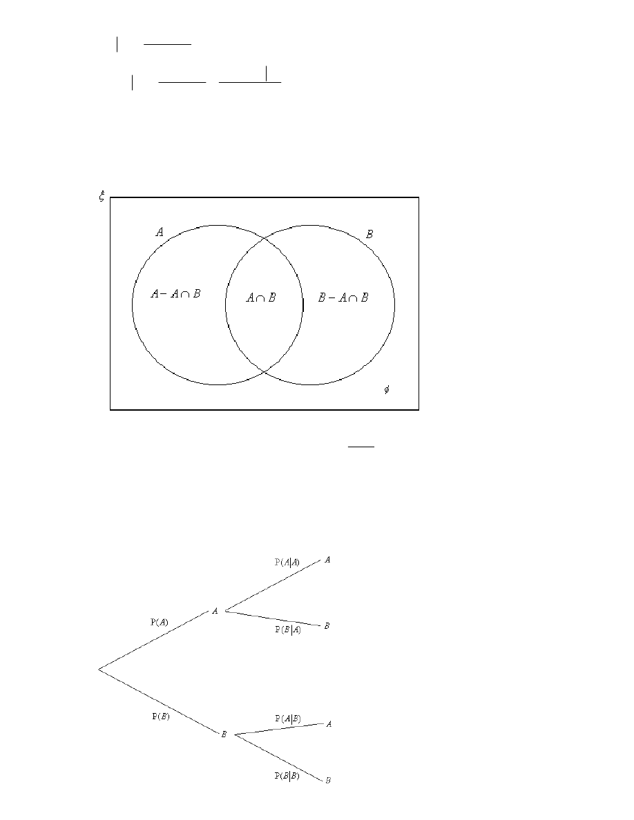
P(
)
P(
)
P( )
P( )P(
)
P(
)
P(
)
P( )
P( )
A B
A B
B
B
A B
A B
B A
A
A
Chapter 6.8 – Use of Venn diagrams, tree diagrams and tables of outcomes to solve
problems.
Venn Diagrams
The probability is found using the principle
( )
P( )
( )
n A
A
n U
.
It is important to note that
B
A
B
A
A
A
n
)
(
and
)
o
(
)
(
)
(
)
(
n
B
n
A
n
U
n
.
Tree diagrams
A more flexible method for finding probabilities is known as a tree diagram.

This allows one to calculate the probabilities of the occurrence of events, even where
trials are non-identical (where
)
(
P
)
(
P
A
A
A
), through the product principle.
Tables of outcomes
Refer to H&H p.504-5.
Chapter 6.9 – Concept of discrete and continuous random variables and their probability
distributions. Definition and use of probability density functions. Expected value (mean),
mode, median, variance and standard deviation.
A random variable represents in number form the possible outcomes, which could occur
for some random experiment. For any random variable there is a probability distribution
associated with it.
A discrete random variable involves a
count. Thus, a discrete random variable X has
possible values
1
2
3
, , ,.....
x x x
Thus, finding P(
)
X
x
(the probability distribution of
x) involves listing P( )
i
x for each
value of
i
x .
In random distribution, the expected outcome E( )
X is the mean. The standard deviation,
or Var( ),
X is the square of the distance of X from the mean:
2
2
2
2
Var( ) E(
)
E(
) {E( )}
X
X
X
X
.
2
2
E(
)
i
i
X
x p
for discrete random
variables and
2
2
E(
)
( )d
X
x f x x
for continuous random distribution.
For a discrete random variable, the mode and median can be found as outlined above.
The mean and variance can be expressed as follows:
i
i
x p
2
2
2
2
i
i
i
i
x
p
x p
A continuous random variable involves measurements. A continuous random variable
X
has all possible values in some interval (on the number line).
Rather than a probability distribution, continuous random variables have probability
density functions. A continuous probability function (pdf), ( ),
f x is a function where
( ) 0
f x
on a given interval, such as [a, b] and
( )d
1.
b
a
f x x
For a continuous
probability density function, the mode is that value of
x at the maximum value of ( )
f x on
[
a, b]. The median m, is the solution for m of the equation
1
( )d
2
m
a
f x x
. The mean and
variance can be expressed as follows:
( ) d
x f x
x
2
2
2
2
( )d
( )d
x
f x x
x f x x

It is important to note that standard deviation
2
Var( )
X
The following rules summarise the properties of E( )
X .
E( )
for some constant
E(
)
E( ) for some constant
E( ( )
( )) E( ( )) E( ( )) for functions and
k
k
k
kX
k X
k
A X
B X
A X
B X
A
B
This makes it possible to derive another form for the variance.
Chapter 6.10 – Binomial distribution, its mean and variance. Poisson distribution, its
mean and variance.
Binomial Distribution
In the case of
n trials where there are r successes and n − r failures, P(
)
n
r n r
r
X
r
C p q
where
q = 1 − p and r = 0, 1, 2, 3, 4, …, n.
p is the probability of a success and q is the probability of a failure. P(
)
X
r
is the
probability distribution function.
There are three criteria that must be met in order for a random probability distribution to
be a binomial distribution.
1. The probability distribution is discrete.
2. There are two outcomes – success and failure.
3. The trials are independent – the probability of success is a constant in each trial.
If
x is a random variable which is binomial with parameters n and p, then the mean of x is
np
and the variance of
x is
2
npq
.
Calculator: P(
) binompdf ( , , )
x r
n p r
and P(
) binomcdf ( , , )
x r
n p r
Poisson Distribution
The Poisson distribution is defined as P(
)
!
x
m
m e
X
x
x
where
m is the parameter.
2
f x
m
f
.
2
2
2
2
2
2
2
2
2
2
( ) E(
)
(
2
)
E(
) 2 E( )
E(
) 2
E(
) {E( )}
Var X
X
E X
X
X
X
X
X
X
There are three criteria that must be met in order for a random probability distribution to
be a binomial distribution.
1. The average number of occurrences (
μ) is constant for every interval.
2. The probability of more than one occurrence in a given interval is very small.
3. The number of occurrences in disjoint intervals are independent of each other.
Chapter 6.11 – Normal distribution. Properties of the normal distribution.
Standardization of normal variables.
If
X is normally distributed then its probability density function is given by
2
2
1
2
1
)
(
x
e
x
f
for
x
.
The grand majority of continuous distributions are normal distributions, where the
probability density decreases according to how far the value is from the mean. This is
particularly true for variables in nature.
Properties
The curve is symmetrical about the line
x
0
)
(
lim
x
f
x
1
d
)
(
x
x
f
)
(
Max
x
f
is uniquely determined as the horizontal distance from the vertical distance from the
vertical line
x
to a point of inflection.
In a normal distribution, 68.26% of values lie within one standard deviation of the mean,
95.4% of values lie within two standard deviations of the mean and 99.74% of values lie
within three standard deviations of the mean.
Since
( )
P( )
( )
n A
A
n U
, the probability of
X lying within a certain interval is equal to the
percentage of values that lie within that interval. This is obtained from the data booklet
and from GDCs.
The standard normal distribution, or
Z-distribution, is the application of the
transformation
X
Z
to a normal
X-distribution, such that the mean is at x = 0 and
there is one standard deviation per unit on the
x-axis. Where the probability density
function for normal distribution has two parameters
and
, the
Z-distribution has
none. This makes it useful when comparing results from two or more different normal
distributions, since comparing
Z-values allows one to take into account the standard
deviation and mean when comparing results.
Finding probabilities with a GDC involves using
)
,
,
,
normalcdf(
b
a
for lower limit
a
and upper limit
b (under “DISTR”). It is important to note that
)
(
P
)
(
P
a
Z
a
Z
.
To find probabilities for a normally distributed random variable
X, convert X values to Z
using the transformation, sketch the standard normal curve (shade the required region)
and find the standard normal table or a graphics calculator to find the probability.
)
,
,
(
normalpdf
x
gives the probability for a particular
x-value.

Chapter 7.1 – Informal ideas of limit and convergence. Definition of derivative as
0
lim
.
h
f x h
f x
f x
h
Derivative of
n
x
n
,
sin x
,
cos x
, tan
x ,
x
e and
ln x
. Derivative interpreted as a gradient function and as rate of change. Derivatives of
reciprocal circular functions. Derivatives of
x
a and log
a
x . Derivatives of
arcsin x
,
arccos ,
x arctan x .
All functions approach a particular value as the value of the variable they are in terms of
approaches a given value. However, in certain cases, it is not possible to directly
determine the value of the function at that particular value of the variable because the
answer involves division by zero or the value of the variable in question is, in fact,
infinity. Thus, where a function converges towards a particular value, it can be said that
the limit of the function at that value of the variable is equal to the value the function
approaches.
For example,
sin
0
only where
0
and since the function
sin
is continuous, it
means that for
0,sin
. What is more, since the closest point of inflection to the
sine function occurs at 0, the closer
is to 0, the closer
sin
is to
.
Thus, given the function
sin
f
, the closer
is to 0, the closer
1
f
.
However,
0
0
is undefined. Thus, we can say that since
f
tends towards 1 as
tends
towards 0,
0
sin
lim
, or the limit of
sin
as
tends to 0 is 1.
The derivative,
( )
f x
of a point
( ),
f x x
on a function is the gradient of the tangent – or
instantaneous rate of change of the function – at that point. This can be found by using
the area of limits:
Take two points A and B on the curve of a function
f x
. Let A have coordinates
( ),
f x x
and B,
h units away from A on the x-axis, therefore have coordinates
(
), (
)
f x h
x h
. Thus, the gradient of the arc AB on the curve joining the two lines is
equal to
(
)
( )
(
)
( )
f x h
f x
f x h
f x
x h
x
h
. It can be seen that the closer point B is to A,
the closer the gradient of the arc is to the gradient of the tangent at point A. Expressed
using limit notation, this gives us the equation:
0
( ) lim
h
f x h
f x
f x
h
.
Using this equation to find the derivative of a function at a point is known as finding the
derivative from first principles. This is done by manipulating the equation until
h is taken
out of the denominator, since this will generate exactly the same result as the previous
equation but with the additional solution for where
0
h
, thus telling us what the limit of
the function as
h tends towards 0 is at the point by setting the
0
h
and solving for the
derivative.
This allows us to generate some general rules for the derivatives.

The first of these is the power rule:
Let ( )
n
f x
x
Thus:
1
0
0
1
1
1
1
0
0
1
1
...
...
1
( ) lim
lim
...
...
1
lim
lim
...
...
1
0
1
n
n
n r r
n
n
n
n
h
h
n
n r r
n
n
n r r
n
h
h
n
n
n
n
x
x h
x h
h
x
x h
x
r
f x
h
h
n
n
x h
x h
h
n
n
r
x
x h
h
r
h
n
x
nx
This result is known as the power rule.
Also note:
If ( )
n
f x
ax
,
1
0
0
0
( ) lim
lim
lim
n
n
n
n
n
n
n
h
h
h
a x h
x
x h
x
a x h
ax
f x
a
anx
h
h
h
It is also fairly evident that any constant if ( )
n
f x
ax
k
,
1
( )
n
f x
anx
The following are rules that are important to note:
1
2
( )
( )
( ) sin
( ) cos
( ) cos
( )
sin
( ) tan
( ) sec
( )
( )
1
( ) ln
( )
n
n
x
x
f x
ax
f x
anx
f x
x
f x
x
f x
x
f x
x
f x
x
f x
x
f x
e
f x
e
f x
x
f x
x
When expressed as ( )
f x
, the derivative of ( )
f x suggests the rate of change function.
When expressed as
d
d
y
x
, the derivative of ( )
f x
y
suggests a gradient function. The two
are, however, completely interchangeable, though
d
d
y
x
is by far a more useful and easier
to manipulate form.
This is because
d
d
y
x
represents the point gradient on the curve as the ratio between an
infinitely small displacement d
y in the y-direction and an infinitely small displacement dx
in the
x-direction, representing any given curve as a series of connected infinitely small
line segments with gradient equal to the tangent of the curve at that point.

Because this representation of the gradient of the tangent is in the form of a fraction (of
infinitely small parts), this allows it to be manipulated in such a way as to yield
interesting results.
For instance, where
d
d
y
x
gives the gradient function of a curve whose
y values are in terms
of
x,
1
d
d
d
d
x
y
y
x
gives the gradient function of a curve whose
x-values are in terms of
y. Taking the integral of this function gives you
d
d
d
x
x
y
which is not a very useful
result, however the inverse of this function,
d
d
d
x
y
y
gives us (what used to be)
x in
terms of
y, in other words, the inverse of the function.
To summarise: The inverse of the integral of the reciprocal of the derivative of a function
is equal to the inverse of the function.
The inverse of the reciprocal of the derivative of a function is equal to the derivative of
the inverse of the function.
The above derivatives and the many more required are all in the formula booklet.
Increasing and decreasing functions.
An increasing function has a positive gradient for all
x and a decreasing function has a
negative gradient for all
x. The intervals during which a function is increasing or
decreasing is found by finding the gradient function and using sign diagrams to determine
when the gradient function is positive and when it is negative.
If a curve has gradient function
d
d
y
x
, the normal to the curve has function
d
d
x
y
.
Chapter 7.2 – Differentiation of a sum and a real multiple of functions in 7.1. The chain
rule for composite functions. Application of chain rule to related rates of change. The
product and quotient rules. The second derivative. Awareness of higher derivatives.
An important rule to remember in differentiation is that if:
( )
( ) ...
( )
d
( )
( ) ...
( )
d
y a f x
b g x
c h x
y
a f x
b g x
c h x
x
The chain rule takes advantage of the fractional properties of the gradient equation to
simplify the differentiation of functions such as
( )
n
y
f x
and to allow for the
determination of other related rates of change.
The chain rule is perhaps best described as it is in the formula booklet:
d
d
d
( ), where
( )
d
d
d
y
y
u
y g u
u
f x
x
u
x

d
( ( ))
( )
( ( ))
d
d
( )
( ), ( )
d
y
y
f g x
g x
f g x
x
y
y
f u
u
f u u g x
x
This has a great many applications, not only to allow for the differentiation of more
complicated functions but also to allow for the derivation of many other functions.
The Chain rule also allows for the determination of related rates of change.
d
d
d
d
d
d
v
v
s
t
s
t
is one example of this, where the function for instantaneous acceleration is
using the functions of instantaneous velocity and the equation of speed relative to
displacement.
The product rule can be described in a similarly clear way:
d
d
d
, where
( ),
( )
d
d
d
y
v
u
y uv
u
f x v g x
u
v
x
x
x
As can the quotient rule:
2
d
d
d
d
d
, where
( ),
( )
d
u
v
v
u
u
y
x
x
y
u
f x v g x
v
x
v
Generally speaking, it is safe to say that these are merely equations to be directly applied
to the question as needed.
The second derivative
( )
f x
or
2
2
d
d
y
x
is the derivative of the derivative of the function. It
represents the curvature of the function: the rate at which the gradient is changing in
relation to x. This is useful for reasons outlined in the next chapter.
Higher derivatives, expressed as
d
d
n
n
y
x
or
( )
( )
n
f
x , are the derivatives of the derivative one
order down.
Chapter 7.3 – Local maximum and minimum points. Use of the first and second
derivative in optimization problems.
Local maxima and minima occur where
d
0
d
y
x
and
2
2
d
0
d
y
x
. If
2
2
d
0
d
y
x
for that value of
x, the point is a minimum, if
2
2
d
0
d
y
x
for that value of x, the point is a maximum. These
can therefore be used in optimisation questions where the function for a given parameter
is found and the differentiation applied, such as in cases dealing with profit, area or
volume.

Chapter 7.4 – Indefinite integration as antidifferentiation. Indefinite integral of
1
n
x
n
,
sin x
,
cos x
,
x
e ,
1
x
. The composites of any of these with the linear
function
ax b
.
Indefinite integration gives the general formula for the area under a function from the
origin to x. One form of indefinite integration is antidifferentiation. It can be explained
conceptually in the following way. Seeing as differentiation is the process by which you
divide the infinitely small rise by the infinitely small run at each point, the reverse
process, defined as antidifferentiation, must involve the opposite process, as in finding
the sum the areas of the infinitely small trapeziums under each infinitely small line
segment.
Antidifferentiation is simply the inverse function of differentiation. The antidifferential of
a function is the function which, when differentiated, gives the original function.
When asked to antidifferentiate, ask yourself: What function, when differentiated, would
give me this function?
Integration rules:
1
1
( )
( )
( )
( )
( )
( )
1
1
1
ln
1
1 (
)
1
1
1
ln
( )
( )
n
n
x
x
ax b
ax b
n
n
kf x dx k f x dx
f x
g x
dx
f x dx
g x dx
k dx kx c
x
dx
x
c
n
e
dx
e
c
dx
x c
x
e
dx
e
c
a
ax b
ax b
dx
c
a
n
dx
ax b c
ax b
a
du
f u
dx
f u
du
dx
Chapter 7.5 – Anti-differentiation with a boundary condition to determine the constant
term. Definite Integrals. Area between a curve and the x-axis or y-axis in a given interval,
areas between curves. Volumes of revolution.
If given the value of ( )
f x at a given value of x for the integral of a function, it is possible
to plug in the numbers to determine the constant term c in
( )d
( )
.
f x x
f x
c
( )d
( )
( ) where is the upper limit of and is the lower limit.
b
a
f x x
f b
f a
b
x
a

This gives the area between the curve and the x-axis for those limits. To find the area
between the curve and the y-axis, it is simplest to take the area of the rectangle ( )
f b b
and subtract from that
( )d
b
a
f x x
and the area of rectangle ( )
.
f a
a
It is also possible to
find the area under the curve of the inverse function, i.e.
d
b
a
x y
rather than
d .
b
a
y x
For the volume V of revolution when an area with limits a and b is rotated about the x-
(first case) or y-axis (second case), it is simplest to state the equations:
2
2
d , d
b
b
a
a
V
y x V
x y
Similarly to the usage of rectangles outlined above, cylinders can be used when rotating
an area between the curve and the axis is not the axis of revolution.
If rotating above a line that is not on an axis, it is necessary to use transformations to
transform the axis of rotation onto either the x- or y-axis in order to use the equations
shown above.
Chapter 7.6 – Kinematic problems involving displacement, s, velocity, v, and
acceleration, a.
2
2
d
d
d
d
,
d
d
d
d
s
v
s
v
v
a
v
t
t
t
s
The area under a velocity-time graph represents distance. It can be important to
manipulate derivatives so that they are in the correct form to find the required solution.
This manipulation must not be forgotten.
Chapter 7.7 – Graphical behaviour of functions: tangents and normals, behaviour for
large
;
x
asymptotes. The significance of the second derivative; distinction between
maximum and minimum points. Point of inflexion with zero and non-zero gradients.
The derivative of a function gives the function of its tangent, the negative reciprocal of
the derivative gives the function of its normal or the normal at that point. The derivative
indicates where the function is getting more positive and where it is getting more
negative. Vertical asymptotes occur where the derivative has infinite value and the
equation of the normal has value 0 and horizontal asymptotes occur where the derivative
of the inverse function is infinite or where the tends to zero as x approaches
(and
where the function of the normal approaches infinity).
The second derivative gives the rate of change of the derivative, i.e. the curvature of the
function (whether the function is getting steeper or less steep). At stationary points, if the
second derivative is positive, the stationary point is a minimum, if the second derivative
is negative, the stationary point is a maximum and where the stationary point has second
derivative 0, the stationary point is a point of inflection, given that the third derivative has
a non-zero value.
Chapter 7.8 – Implicit differentiation.

1
1
m
n
m
n
m
n
dy
dy
x y
mx
y
x ny
dx
dx
Chapter 7.9 – Further integration: integration by substitution integration by parts.
Integration by substitution involves taking
( ( ))d
g f x
x
, replacing ( )
f x by u and
multiplying by
d
d
u
x
. This is derived through reverse application of the chain rule. The part
of the function chosen to serve as u depends on the situation and a feel for it can best be
obtained through practice. CHAPTER 29 H&H
Integration by parts involves the use of the equation:
d
d
d
d
d
d
v
u
u
x uv
v
x
x
x
Sometimes it may be necessary to do repeated integration by parts to obtain the answer.
Chapter 7.10 – Solutions of first order differential equations by separation of variables.
This is best understood by referring to exercise 29D in H&H. It is best summarised as
shown:
d
d
1
d
d
1
d
d
d
d
1
d
d
1
ln
ln
kcx kq
k kcx
y
ky c
x
y
c
ky
x
y
x c x
ky
x
y
c x
ky
y cx q
k
y kcx kq
y e
A e
This is not a general equation however the general method can be used to solve other
types of equation.
Wyszukiwarka
Podobne podstrony:
Mathematics HL P1 May 1995
Mathematics HL May 2004 TZ1 P1
Mathematics HL May 2003 P1
Mathematics HL November 2008P3 Sets
Mathematics HL Nov 2002 P1 $
MATHEMATICS HL May 1999 P1
Mathematics HL Nov 2006 TZ1 P2$
Mathematics HL November 2008P3 Stats M
Mathematics HL paper 3 discrete mathematics
May 1998 Mathematics HL P1$
Mathematics HL May 2004 TZ1 P2 $
Mathematics HL Nov 2004 P1 $
Mathematics HL Nov 2002 P2
Mathematics HL Nov 2006 TZ1 P1
Mathematics HL May 2004 TZ2 P1 $
Mathematics HL May 2004 TZ2 P2
MATHEMATICS HL May 1999 P2$
Mathematics HL May 2004 TZ1 P1 $
więcej podobnych podstron