Image Processing

with MatLab

Professor

Valery Starovoitov

2

Matlab

• A high-level language for matrix

calculations, numerical analysis, &
scientific computing

• Language features

– Intepreted
– No variable declarations
– Automatic memory management
– Vectorized: Can use

for

loops, but largely

unnecessary

3

How to Get Help

• In Matlab

– Type “

help

” to get a listing of topics

– “

help <topic>

” gets help for that topic.

The information is at the level of a Unix man

page

• On the web

– “Matlab links” on course web page has

pointers

– Especially MathWorks help desk:

www.mathworks.com/access/helpdesk/help/helpdesk.shtml

4

Entering Variables

• Entering a scalar, vector, matrix

>> a = 27;
>> V = [10, 4.5, a];
>> M = [3, 4 ; -6, 5];

• Without semi-colon, input is echoed (this is

bad when you’re loading images!). You can

use this as a kind of print statement, though

• Comma to separate statements on same line
• size: Number of rows, columns

5

Constructing Matrices

• Basic built-ins:

– All zeroes, ones: zeros(n) (square

matrix) or zeros(n, m); similarly ones

– Identity (all zeros but ones on

diagonal): eye

– Random: rand (uniform), randn (unit

normal)

• Ranges: m:n, m:i:n (i is step size)

6

More Ways to Make Matrices

• Composing big matrices out of small

matrix blocks

• repmat(A, m, n): “Tile” a big matrix with

m x n copies of A

• Loading data: M = dlmread(‘filename’,

‘,’) (e.g., comma is delimiter)

– Write with dlmwrite(‘filename’, M, ‘,’)

7

Manipulations &

Calculations

• Transpose (‘), inverse (inv)
• Matrix arithmetic: +, -, *, /, ^

– Can use scalar a * ones(m, n) to make matrix of a’s
– repmat(a, m, n) can be faster for big m, n

• Elementwise arithmetic: .*, ./, .^
• Relations: >, ==, etc. compare every element to

scalar

– M > a returns a matrix the size of M where every

element greater than a is 1 and everything else is 0

• Functions

– Vectorized
– sin, cos, etc.

8

Deconstructing Matrices

• Indexing individual entries by row, col:

A(1, 1) is upper-left entry

• Ranges: e.g., A(1:10, 3), A(:, 1)
• Matrix to vector and vice versa by column:

V = M(:), M(:) = V

– Transpose to use row order

• find: Indices of non-zero elements

– find(M==a) gives indices of M’s elements that

are equal to a

9

Vector/Matrix Analysis

• norm (magnitude), max

,

min, sum

• Operates on whole vector
• Works on each column of a matrix

– E.g., max(M) returns vector, each element

of which is the max of a column of M

– max(max(M)) is maximum element of

matrix M

– To operate on rows: Transpose matrix

then do column analysis

10

M-Files

• Any text file ending in “.m”
• Use path or addpath to tell Matlab

where code is (non-persistent?)

• Script: Collection of command line

statements

• Comment: Start line with %

11

Functions

• Function: Define in its own .m file
• Take argument(s), return value(s).

First line defines:

>> function y = foo(A)
>> function [x, y] = foo2(a, M, N)

12

Control Structures

• Expressions, relations (==, >, |, &,

functions, etc.)

• if/while expression statements end

– Use comma to separate expression from

statements if on same line

>> if a == b & isprime(n), M = inv(K);

else M = K; end

• for variable = expression statements end

>> for i=1:2:100, s = s / 10; end

13

Plotting Curves

• 2-D: One vector for each coordinate:

plot(x,y)

– Sine function:
>> plot(0:0.01:2*pi, sin(0:0.01:2*pi))
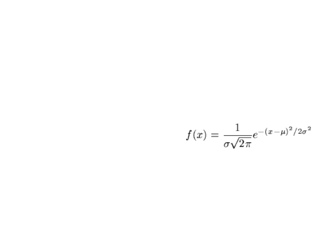
– 1-D normal distribution (“Gaussian”)

with mean

¹

, variance

¾

2

>> Y = (1/sqrt(2*pi*sigma^2))*

exp(-(X-mu).^2/(2*sigma^2));

• 3-D (space curve): plot3(x, y, z)

14

Plotting Options

• Manipulate axes with axis, add to

existing plot with hold on

• Control behavior of plot with

optional 3

rd

argument

– Isolated points vs. connected, size

and color of points & lines, etc.

– Default (no 3

rd

argument) is

connected points

– Get details with help plot

15

Plotting Surfaces

• Surfaces

– meshgrid makes surface from axes,

mesh plots it

>> [X,Y] = meshgrid(-2:.2:2,

-2:.2:2);

>> Z = X .* exp(-X.^2 - Y.^2);
>> mesh(Z)

–surf: Solid version of mesh

16

Saving Figures

• Use print –dpng filename or –

djpgnn, where nn is quality 00-99

17

Images

• Reading: I = imread(‘filename’);
• Accessing/modifying the pixels

– I is m x n if image is grayscale — e.g., I(i,j)
– I is m x n x 3 if image is color — e.g.,I(i,j,1)

• Writing: imwrite(I, ‘filename’);

18

Displaying Images

• Just the image: imshow(I);
• With overlay:

I = imread(‘gore5.jpg');
[r,c,d]=size(I);
imshow(I), hold on;
plot(c*rand(100,1),r*rand(100,1),

'r*');

hold off;

19

Performance Issues

• “Pre-allocate” matrices, vectors

when possible by creating them with
zeros, ones, etc.

• Try to avoid for loops as much as

possible by using vectorized
functions

20

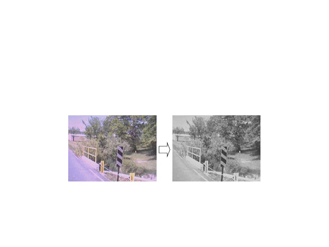
Image Type Conversions

• Many Matlab functions work on just one channel

– Run on each channel independently
– Convert from color  grayscale weighting each

channel by perceptual importance (rgb2gray)

• Some operations want the pixels to be real-

valued

– Type conversion: I2 = double(I1)

21

Image Arithmetic

• Just like matrices, we can do pixelwise arithmetic

on images

• Some useful operations

– Differencing: Measure of similarity
– Averaging: Blend separate images or smooth a single

one over time

– Thresholding: Apply function to each pixel, test value

• In Matlab: imadd, imsubtract, imcomplement,

imlincomb, etc.

– Beware of truncation
– Can do all of these with matrix operations if you pay

attention to types and truncation

22

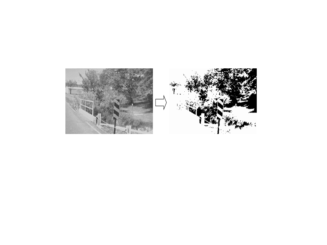
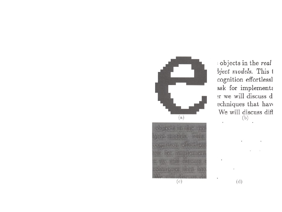
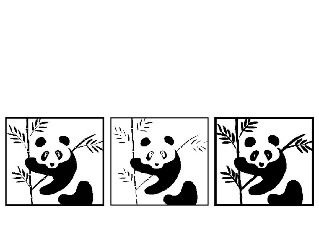
Thresholding

• Grayscale  Binary: Choose threshold

based on histogram of image intensities

(Matlab: imhist)

23

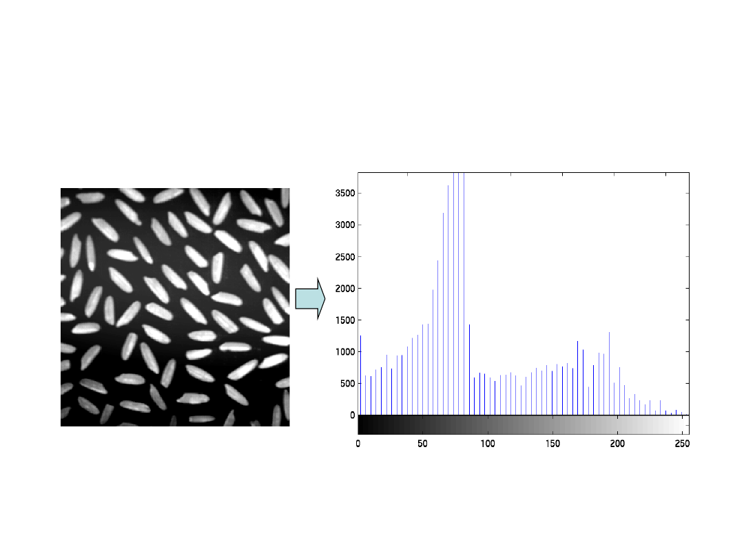
Image Comparison:

Image Histograms

24

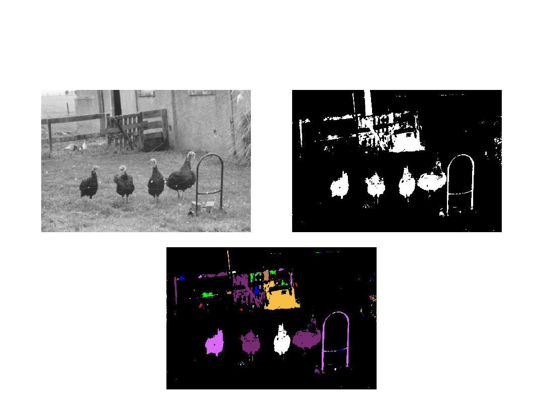
Derived Images: Color

Similarity as Chrominance

Distance

• Distance to red in YIQ space

(rgb2ntsc)

• Can threshold on this

25

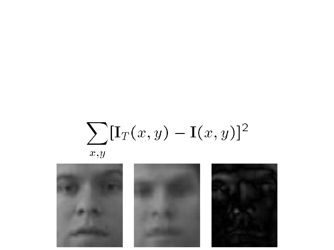
Geometric Image Comparison:

SSD

• Given a template image

I

T

and an image

I

,

how to quantify the similarity between
them?

• Vector difference:

Sum of squared

differences (SSD)

26

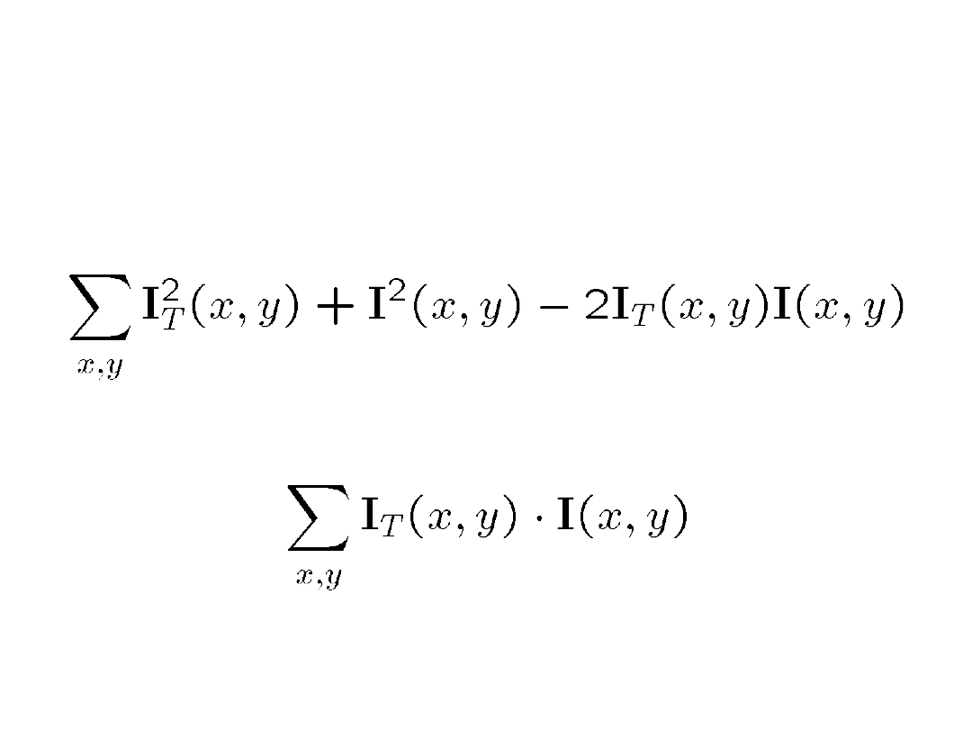
Correlation for

Template Matching

• Note that SSD formula can be written:

• When the last term is big, the mismatch is

small—the dot product measures
correlation:

• By normalizing by the vectors’ lengths, we

are measuring the angle between them

27

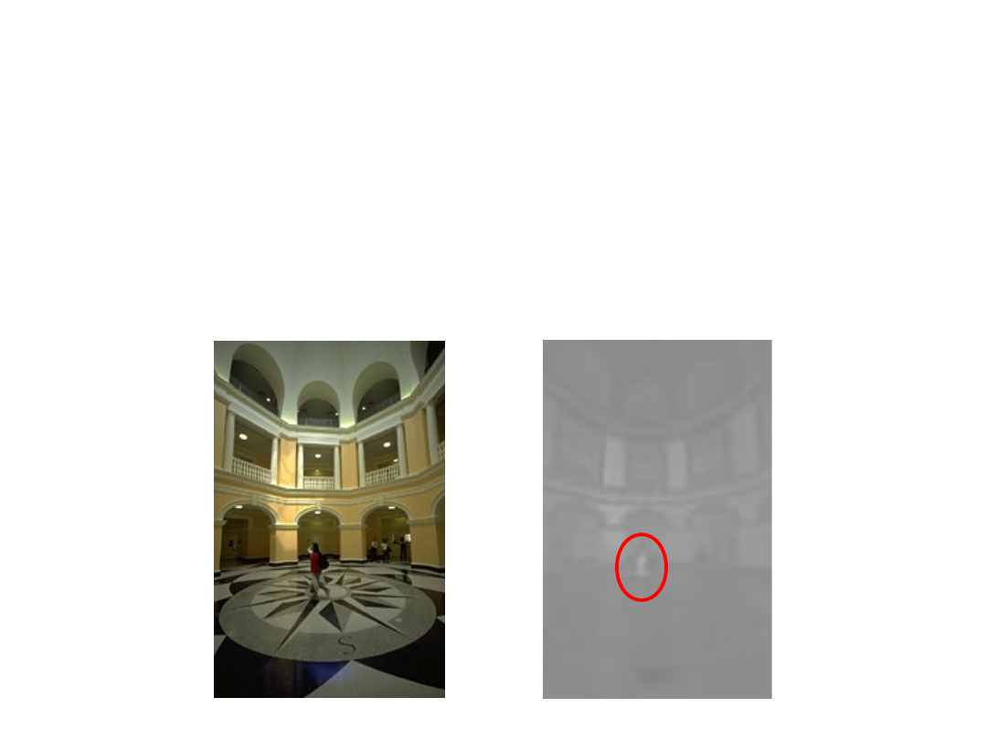
Normalized Cross-

Correlation

• Shift template image

over search image,
measuring normalized
correlation at each
point

• Local maxima

indicate template
matches

• Matlab: normxcorr2

28

Statistical Image Comparison:

Color Histograms

• Steps

– Histogram RGB/HSI triplets over two images to be

compared

– Normalize each histogram by respective total

number of pixels to get frequencies

– Similarity is Euclidean distance between color

frequency vectors

• Insensitive to geometric changes, including

different-sized images

• Matlab: imhist, hist

29

Connected Components

• After thresholding, method to identify

groups or clusters of like pixels

• Uniquely label each n-connected

region in binary image

• 4- and 8-connectedness
• Matlab: bwfill, bwselect

30

Example: Connected

Components

31

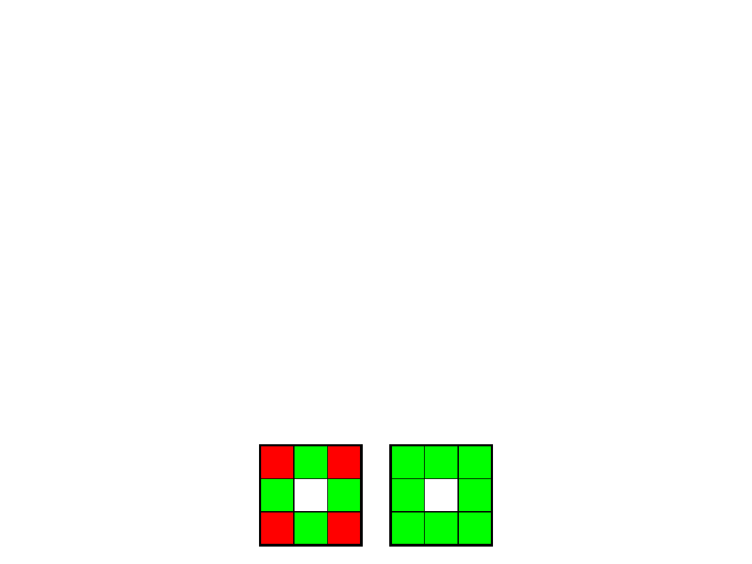
Binary Operations

• Dilation, erosion (Matlab: imdilate,

imerode)

– Dilation: All 0’s next to a 1  1 (Enlarge

foreground)

– Erosion: All 1’s next to a 0  0 (Enlarge

background)

Original

Dilated

Eroded

32

Moments: Region Statistics

• Zeroth-order: Size/area
• First-order: Position (centroid)
• Second-order: Orientation

33

What to read?

• The MathWorks Matlab documentation

http://www.mathworks.com

• Matlab Tutorial

ttp://www.cyclismo.org/tutorial/matlab/

• Matlab

http://www.math.utah.edu/lab/ms/matlab/matlab.html

• Computer Vision (2 lectures)

http://vision.cis.udel.edu/cv