Survivable Networks

Lecture Outline

• Introduction
• Failure State Modeling
• Link Protection
• Path Protection
• Restoration
• Survivable P2P Multicasting
• Concluding Remarks

Lecture Outline

• Introduction

• Failure State Modeling
• Link Protection
• Path Protection
• Restoration
• Survivable P2P Multicasting
• Concluding Remarks

Introduction

• Current computer networks have links of Gbps or

even Tbps capacity

• A failure of a 10Gbps link of 1 second duration

leads to the lost of 1.25GB of data

• Computer networks play a very significant role in

modern world – a network failure can cause many

severe consequences including such areas as

business, politics, society, health

• To protect the network against possible failures,

special design methods are necessary

Failure Causes

• Internal versus external causes, depending on

whether the failure is caused by a network-internal
imperfection or by some surrounding event

• Examples of internal causes: system design

errors, defects of electronic or optical components,
a battery breakdown, human (worker) error

• Examples of external causes: electricity

breakdown, hurricane, lightning, storm,
earthquake, flood, digging accident, vandalism, or
sabotage

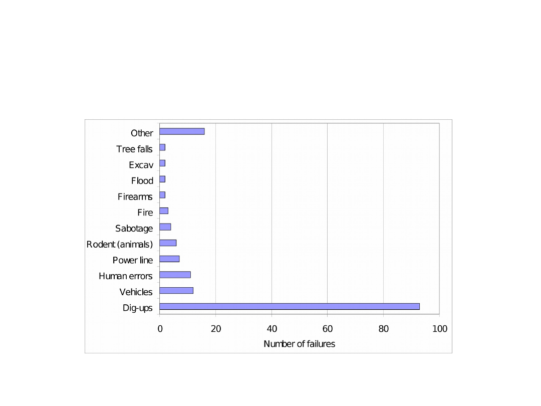
Cause Breakdown for Fibers

[Dan Crawford. "Fiber optic cable dig-ups - causes and cures". Network Reliability and Interoperability Council website. 1992]

Outage Time Impacts (1)

Duration

Main Effects / Characteristics

<50 ms

No outage logged: system reframes,

service "hit", 1 or 2 error-seconds

(traditional performance spec for APS

systems), TCP recovers after one errored

frame, no TCP fallback. Most TCP sessions

see no impact at all

50 ms – 200

ms

< 5% voiceband disconnects, signaling

system (SS7) switch-overs, SMDS (frame-

relay) and ATM cell-rerouting may start

Outage Time Impacts (2)

Duration

Main Effects / Characteristics

200 ms – 2 s

Switched connections on older channel

banks dropped (CGA alarms) (traditional

max time for distributed mesh

restoration), TCP/IP protocol backof

2 s – 10 s

All switched circuit services disconnected.

Private line disconnects, potential data

session / X.25 disconnects, TCP session

time-outs start, web page not available

errors. Hello protocol between routers

begins to be afected

Outage Time Impacts (3)

Duration

Main Effects / Characteristics

10 s- 5 min All calls and data sessions terminated.

TCP/IP application layer programs time
out. Users begin attempting mass redials /

reconnects. Routers issuing LSAs on all
failed links, topology update and
resynchronization beginning network-wide

5 min – 30

min

Digital switches under heavy reattempts

load, "minor" societal / business efects,
noticeable Internet "brownout."

Outage Time Impacts (4)

Duration

Main Effects / Characteristics

>30 min

Regulatory reporting may be required.
Major societal impacts. Headline news.
Service Level Agreement clauses

triggered, lawsuits, societal risks: 911,
travel booking, educational services,
financial services, stock market all

impacted

Protection Methods

• Reliable networks built using elements with low

probability failure (or high probability to be fully
operational during a certain time frame)
expressed by e.g., MTBF (mean time between
failures)

• Since each element has some (even very low)

probability failure, then the network should be
survivable

• The basic mechanism to provide the network

survivability is redundancy of network elements
(e.g., links, routers, etc.)

Definitions

• Network survivability it is the ability of a

network to recover the traffic in the event of a
failure to minimize consequences of the failure for
the users

• As it is impossible for a network to be completely

survivable (e.g., in the case of major earthquakes
causing multiple failures in the network), we use
the degree of survivability

• The self-healing network can itself detect the

failure and reconfigure its resources to minimize
the failure impact

Survivability Approaches (1)

• In order to provide network survivability two

methods are used: protection and restoration

• Protection needs preallocated network

resources

• Restoration applies dynamic resource

allocation

• The distinction between protection and

restoration consists also in the different time
scale in which they operate, protection provides
much faster reaction to the failure

Survivability Approaches (2)

• Automatic protection switching (APS) uses

dedicated backup elements in the network with

automatic switching mechanisms:

– 1+1 one working system and a completely

reserved backup system in which the transmit

line signal is copied

– 1:1 APS is similar to 1+1 but the transmit

signal is not kept in the bridged state

– 1:N denotes that N working systems share one

standby "protection" system

Survivability Approaches (3)

• Self-healing rings – various versions of the ring

topology are used to provide survivability

• Flooding algorithms – after a failure, the

afected data is sent through the network using

flooding algorithms

• Path protection/restoration – a network

connection (e.g., LSP in MPLS) is protected by a

backup path

• Span (link) protection/restoration – a network

span (link) is protected by backup path(s)

• P-cycles – special ring structures

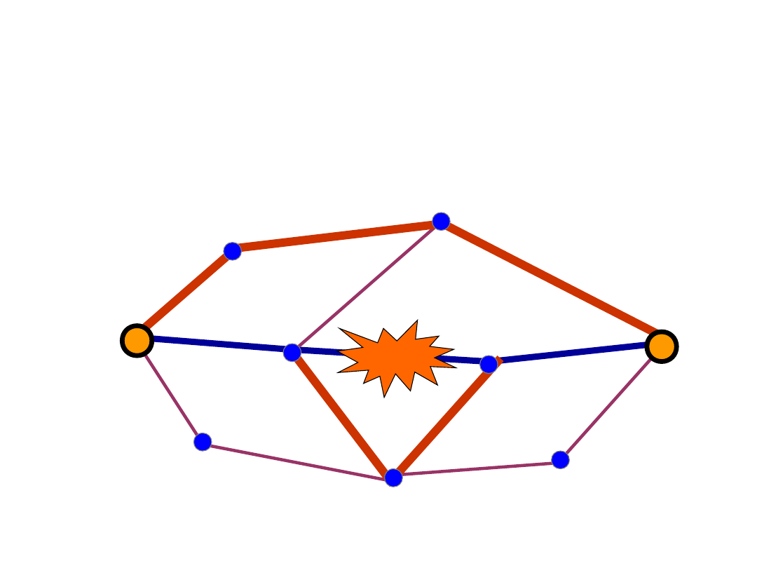
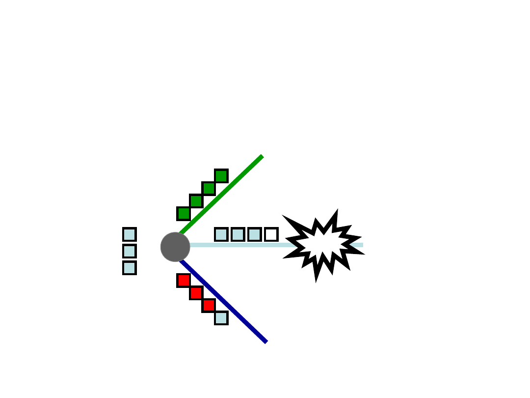
Path and Span Protection

• Path protection/restoration

• Span protection/restoration

Lecture Outline

• Introduction

• Failure State Modeling

• Link Protection
• Path Protection
• Restoration
• Survivable P2P Multicasting
• Concluding Remarks

Failure State Modeling (1)

• Each network failure state (situation) s = 1,2,

…,S is characterized by a vector of link

availability coefficients



s

= (



1s

,



2s

,..,



Es

),

where 0 



es

 1

• Each coefficient



es

determines a proportion of

the normal capacity y

e

of link e,



es

y

e

, that is

available on link e in situation s

• Frequently, the availability coefficients



es

are

binary

• A common practice is a single link failure (only

one link can fail at a time), however other

scenarios can be easily modeled

Failure State Modeling (2)

• Failure situations are also characterized by

vectors of demand coefficients



s

= (



1s

,



2s

,..,



Ds

)

• Each coefficient



ds

determines the proportion of

the reference demand volume h

d

of demand d,

h

ds

=



ds

h

d

, that must be realized in situation s

• The demand coefficients can denote that the

volume of demand d realized in failure situation

s can be decreased, i.e.,



ds

< 1

• The case of when



s

= 1 means that there is

100% demand protection/restoration

Failure State Modeling (3)

• The normal state (without any failure) can be

denoted by s = 0 and characterized with



e0

= 1 and



d0

= 1

• The demand volume at the normal network operating

state becomes the reference demand volume

• The most common failure is the link failure, in this

case we have S = E failure states and



es

= 0 if s = e

and



es

= 1 if s  e

• In the case of a node failure v, we set



es

= 0 for all

links adjacent to node v and set



ds

= 0 for all

demands orignating or terminating in node v

Lecture Outline

• Introduction
• Failure State Modeling

• Link Protection

• Path Protection
• Restoration
• Survivable P2P Multicasting
• Concluding Remarks

Link Protection (1)

• CFA (Capacity and Flow Assignment) problem
• Bifurcated unicast flows (e.g., IP protocol)
• Link protection method
• Single link failure
• Objective is to minimize network cost including

normal and spare capacity

• Modular capacity

Link Protection ( 2)

Given: network topology, unicast demands,

candidate paths for demands and backup paths

for links, link protection

Minimize: network cost of normal and spare

capacity

Over: bifurcated flows (routing), link capacity

Link Protection (3)

indices
d = 1,2,…,D

demands

p = 1,2,…,P

d

candidate paths for demand d

e,l = 1,2,…,E

links

q = 1,2,…,Q

e

candidate paths for protection of

link e

Link Protection (4)

constants



edp

= 1, if link e belongs to path p realizing

demand d; 0, otherwise

h

d

volume of demand d



e

unit (marginal) cost of link e



leq

= 1, if link l belongs to path q protecting link

e;

0, otherwise

M

size of the link capacity module

Link Protection (5)

variables
x

dp0

flow allocated to path p of demand d in

normal state

(no failures) of the

network(continuous non-

negative)

y

e

normal capacity of link e (integer non-

negative)

z

eq

flow restoring normal capacity of link e on

restoration

path q

y´

e

spare capacity of link e (integer non-negative)

Link Protection (6)

objective
minimize 

e



e

(y

e

+ y´

e

)

constraints


p

x

dp0

= h

d

, d = 1,2,…,D



d



p



edp

x

dp0

 My

e

, e = 1,2,…,E



q

z

eq

= My

e

, e = 1,2,…,E



q



leq

z

eq

 My´

l

, l = 1,2,…,E e = 1,2,…,E; l  e.

Optimization

• The problem is linear, integer and NP-

complete

• To find optimal solution branch-and-bound or

branch-and-cut algorithm must be constructed

• The solution process can be divided into two

phases: normal capacity and next spare capacity

• Other heuristics can be used

Lecture Outline

• Introduction
• Failure State Modeling
• Link Protection

• Path Protection

• Restoration
• Survivable P2P Multicasting
• Concluding Remarks

Path Protection (1)

• CFA (Capacity and Flow Assignment) problem
• Bifurcated unicast flows (e.g., IP protocol)
• Path protection method
• Failure scenario modeling
• Objective is to minimize network cost of

capacity

• Modular capacity

Path Protection ( 2)

Given: network topology, unicast demands,

candidate paths, failure states, path protection

Minimize: network cost of normal and spare

capacity

Over: bifurcated flows (routing), link capacity

Path Protection (3)

indices
d = 1,2,…,D

demands

p = 1,2,…,P

d

candidate paths for demand d

e = 1,2,…,Elinks
s = 1,2,…,S failure states

Path Protection (4)

constants



edp

= 1, if link e belongs to path p realizing

demand d; 0, otherwise

h

d

volume of demand d



e

unit (marginal) cost of link e



ds

demand coefficient of demand d in state s,

h

ds

=



ds

h

d



es

fractional availability coefficient of link e in

state s

(0 



es

 1)

M size of the link capacity module

Path Protection (5)

variables
x

dps

flow allocated to path p of demand d in state

s

y

e

capacity of link e (integer non-negative)

objective
minimize 

e



e

y

e

constraints


p

x

dps

= h

ds

, d = 1,2,…,D s = 0,1,2,…,S



d



p



edp

x

dps

 M



es

y

e

, e = 1,2,…,E s = 0,1,2,…,S.

Optimization

• The problem is linear, integer and NP-

complete

• To find optimal solution branch-and-bound or

branch-and-cut algorithm must be constructed

• Heuristics can be used

Lecture Outline

• Introduction
• Failure State Modeling
• Link Protection
• Path Protection

• Restoration

• Survivable P2P Multicasting
• Concluding Remarks

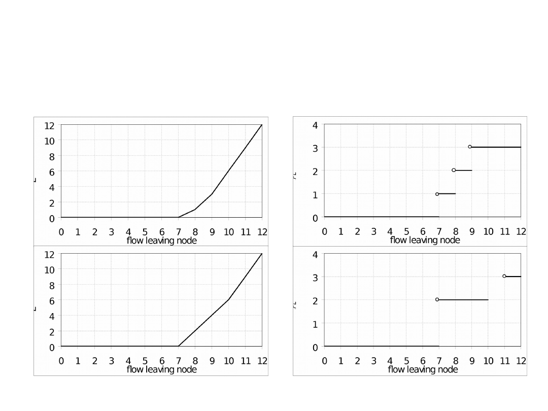
Function LFL (1)

• A projected traffic demand and link capacity is

given

• Link restoration strategy is applied, in which

the upstream node of the failed link is responsible

for the rerouting of the broken connection

• LFL (Lost Flow in Link) function should enable

efficient optimization of primary routes for local

restoration

• Two functions were proposed for optimization of

primary routes using the local restoration:

– Maximum flow algorithm, complexity O(V

3

) for one linke

– KSP (k-shortest path) O(VlogV) for one link

Function LFL (2)

Function LFL (3)

f

flow vector, f = [f

1

, f

2

,… f

E

]

c

e

capacity of link e

out(e) links leaving the origin node of link e, except e
in(a)

links entering destination node of link e, except e

2

/

)

(

)

(

)

(

)

(

in

)

(

out





































































e

i

i

i

e

e

i

i

i

e

e

c

f

f

c

f

f

LFL f















0

for

0

for

0

)

(

x

x

x

x





e

e

LFL

LFL

)

(

)

(

f

f

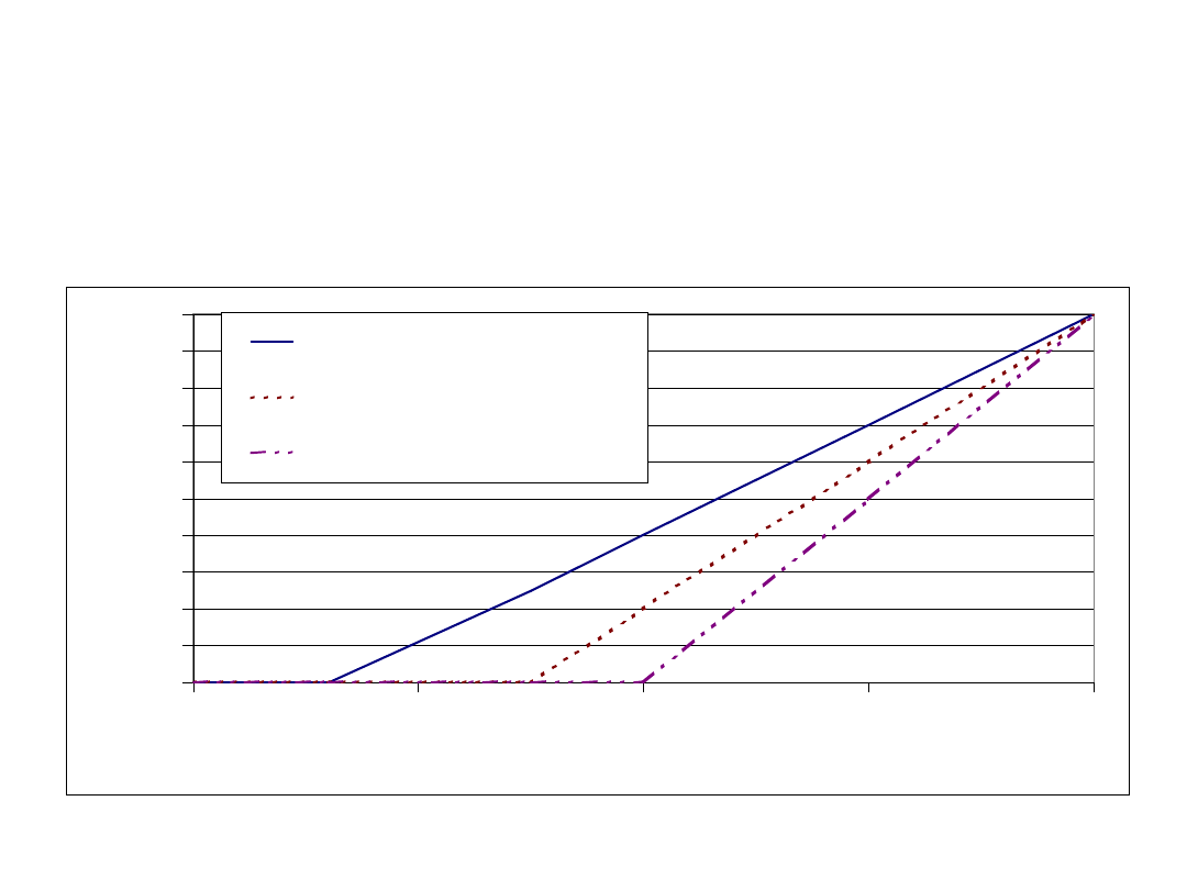
Function LFL (4)

0

100

200

300

400

500

600

700

800

900

1000

0.6

0.7

0.8

0.9

1

Average Link Utilization

T

h

e

o

re

ti

c

cu

rv

e

s

o

f

L

F

L

Average Node Degree=3.0

Average Node Degree=4.0

Average Node Degree=5.0

Function RCL (1)

• Function RCL (Residual Capacity with LFL)

combines the LFL function derivative and link
residual capacity









e

e

e

LFL

e

f

c

l

RCL

)

(

1

)

(

f

f

Function RCL (2)

Optimization Problem (1)

• FA (Flow Allocation) problem
• Non-bifurcated flows (e.g., MPLS)
• Link-path formulation
• Working paths are optimized according to a

selected function (e.g., LFL, RCL, Delay) to enable
efective restoration

• After single link failure , restoration is applied
• Next the lost flow is calculated (volume of not

restoraed demands)

Optimization Problem (2)

Given: network topology, link capacity, unicast

demands, candidate paths

Minimize: LFL, RCL, congestion (CNG), relative

congestion (CNG), delay (DEL)

Over: Non-bifurcated routing

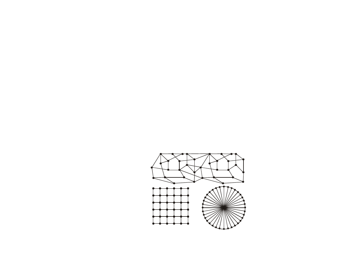
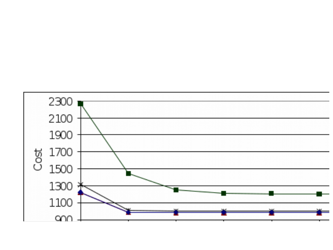
Results

• Various 36-node networks are tested
• All links have the capacity 4800
• In experiment A, there is a demand for every

node pair

• In experiments B and C, 2500 random

demands are generated

1 2 0 m e s h

1

3

4

5

6

2

7

9

1 0

1 1

1 2

8

1 6

1 7

1 8

1 3

1 4

1 5

2 2

2 3

2 4

1 9

2 0

2 1

2 8

2 9

3 0

2 5

2 6

2 7

3 4

3 5

3 6

3 1

3 2

3 3

1

1 0

2 8

1 9

2

3

4

6

7

8

9

5

3 6

3 5

3 4

3 2

3 1

3 0

2 9

3 3

2 0

2 1

2 2

2 4

2 5

2 6

2 7

2 3

1 8

1 7

1 6

1 4

1 3

1 2

1 1

1 5

1 0 8 r i n g

1 2 8

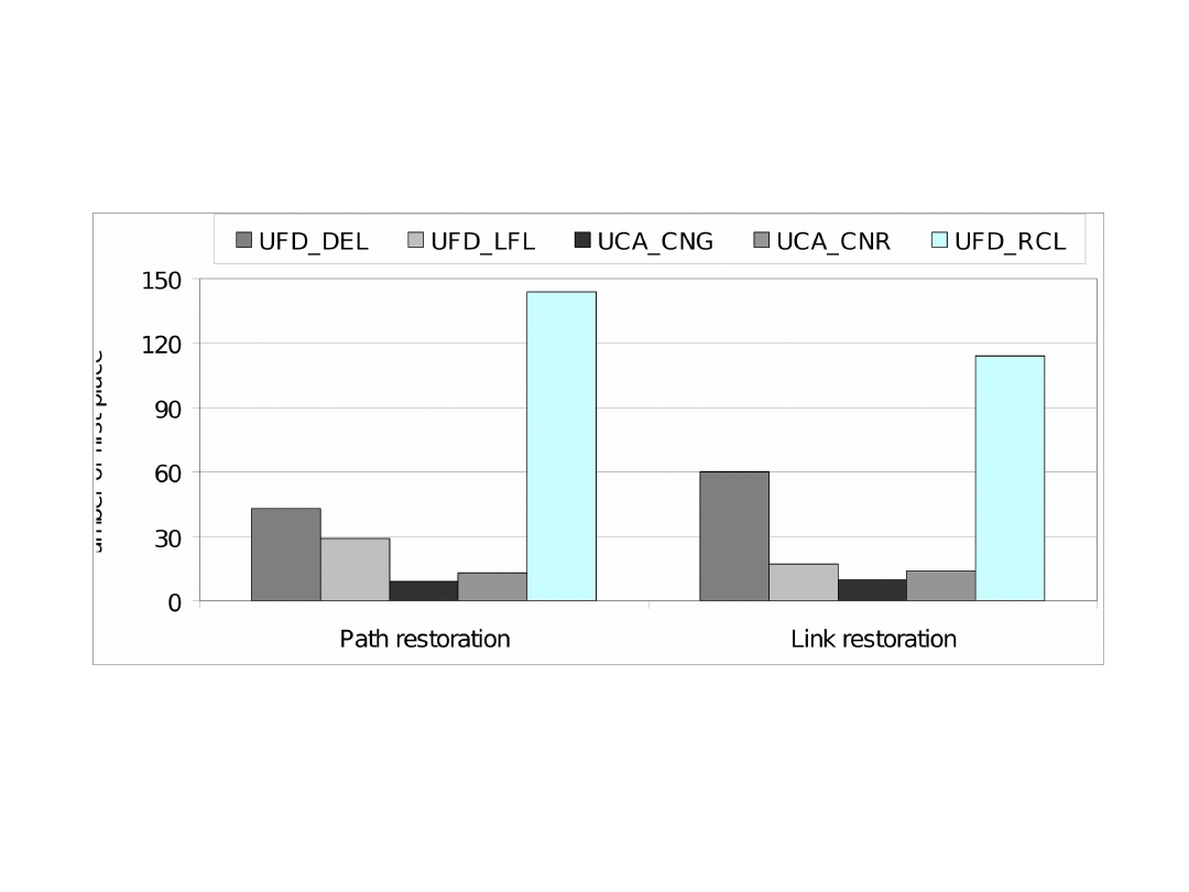
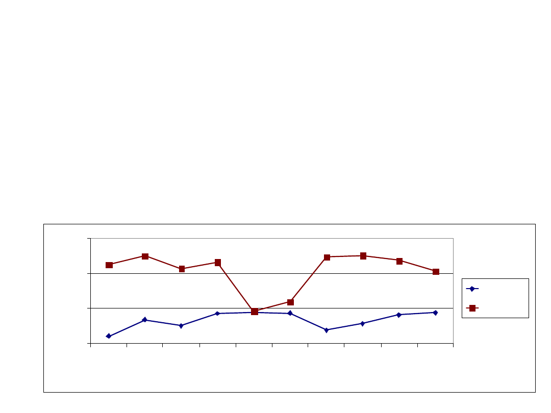
Comparison of Functions (1)

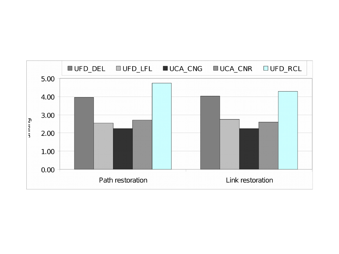
Comparison of Functions (2)

Lecture Outline

• Introduction
• Failure State Modeling
• Link Protection
• Path Protection
• Restoration

• Survivable P2P Multicasting

• Concluding Remarks

Survivable P2P Multicasting

(1)

• Failure-disjoint trees transmitting the same

content simultaneously (inspiration from
protection methods developed for computer
technologies like MPLS, DWDM)

• Each receiver (peer) downloads the stream using

at least two failure-disjoint trees

• In the case of a failure peers afected by the

failure of one of the trees can use another
tree(s) to receive the required data

• This procedure guarantees very low restoration

time

Survivable P2P Multicasting

(2)

We consider three kinds of failures:
• Overlay link failure - a pair of peers is

disconnected. If there was a transfer on this link,

some downstream nodes are afected by the

failure. The overlay link failure comprises failure

of both directed links

• Uploading node failure - impacts all successors

of the failed peer in the tree. Therefore, we focus

only on failure of nodes that have some children

• ISP link failure - means, that all overlay links

between peers of one ISP and peers of the second

ISP are not available

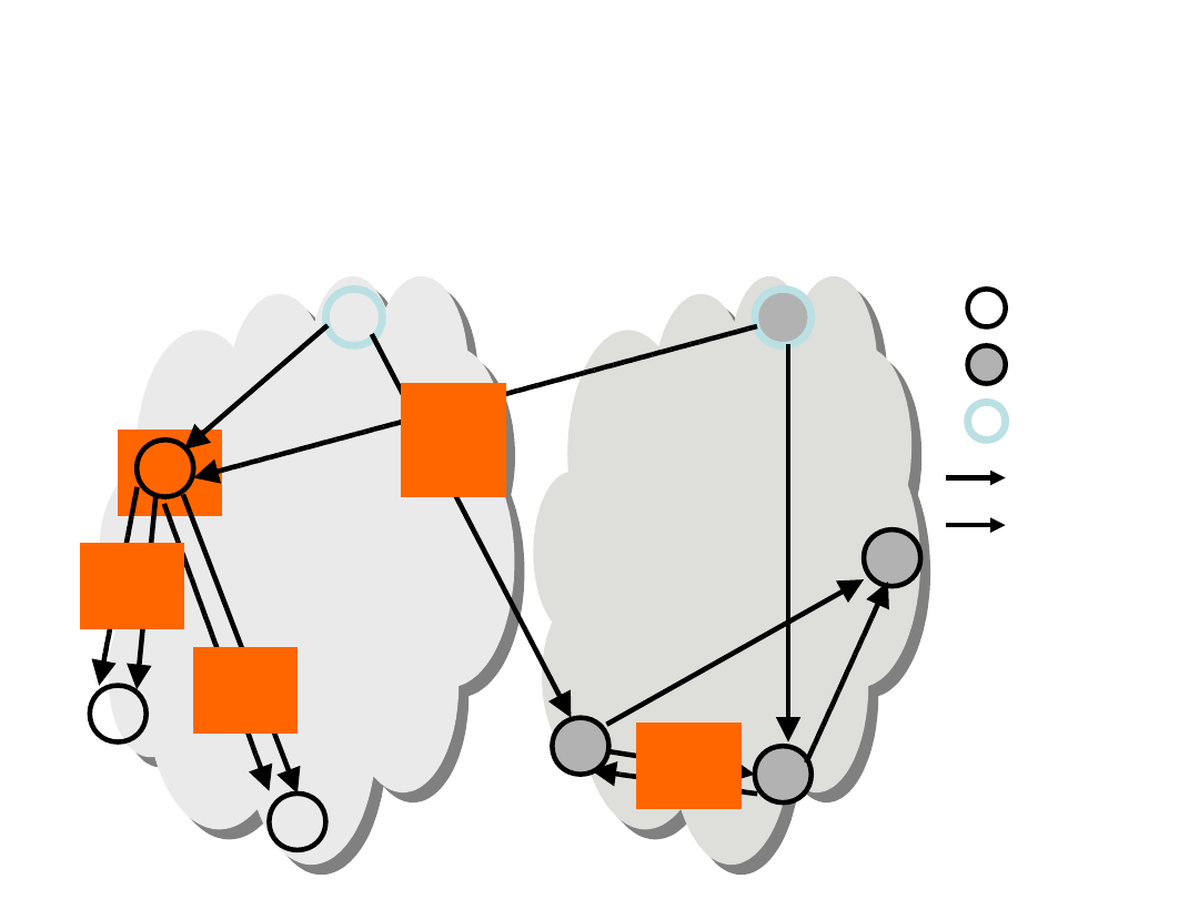
Survivable P2P Multicasting

(3)

ISP1
ISP2
Root
Tree A
Tree B

a

c

ISP1

ISP2

e

d

b

f

g

h

a

b

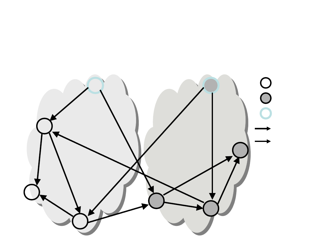
Survivable P2P Multicasting

(4)

ISP1
ISP2
Root
Tree A
Tree B

a

c

ISP1

ISP2

e

d

b

f

g

h

a

b

Survivable P2P Multicasting

(5)

• FA (Flow Assignment) problem
• P2P multicast flows
• Overlay network
• Disjoint tree protection method
• Failures: overlay link, uploading node, ISP link
• Objective is to minimize cost

Survivable P2P Multicasting

(6)

Given: network topology, root location, number of

disjoint trees, streaming rates, protection
scenario

Minimize: streaming cost

Over:P2P multicast routing

Survivable P2P Multicasting

(7)

indices
w,v = 1,2,…,V

overlay network nodes (peers)

k = 1,2,…,K

receiving nodes

t = 1,2,…,T

trees

l = 1,2,…,L

levels of the multicast tree

Survivable P2P Multicasting

(8)

constants
d

v

download capacity of node v

u

v

upload capacity of node v

r

vt

= 1, if node v is the root of tree t; 0, otherwise

q

tree streaming rate (bps)

c

wv

streaming cost of overlay link (w,v)

M

large number

Survivable P2P Multicasting

(9)

variables
x

wvtl

streaming rate on an overlay link (w,v) (no

other

peer nodes in between) in multicast

tree t and w is located on level l of tree t;

(continuous, non-

negative)

y

vwt

= 1, if link from node w to node v (no other

peer

nodes in between) is in multicast tree t;

0 otherwise;

(binary)

objective
minimize 

w



v



t

 y

wvt

c

wv

Survivable P2P Multicasting

(10)

constraints


w



l

 x

wvtl

 = 0   v = 1,2,…,V   t = 1,2,…,T   r

vt

 = 1



w



l

 x

wktl

 = q   k = 1,2,…,K   t = 1,2,…,T



v

 x

wvt1

  u

w

r

wt

   w = 1,2,…,V   t = 1,2,…,T

x

wvt(l+1)

  

b

 x

bwtl

   v = 1,2,…,V   w = 1,2,…,V

t = 1,2,…,T  l = 1,2,…,L – 1

Survivable P2P Multicasting

(11)

constraints


w



t



l

 x

wvtl

 



 d

v

   v = 1,2,…,V



v



t



l

 x

wvtl

  u

v

   w = 1,2,…,V



v



t



l

x

vvtl

 = 0



l

x

wvtl

  qy

wvt

  v = 1,2,…,V w = 1,2,…,v  t = 1,2,…,T

y

wvt

  

l

x

wvtl

 v = 1,2,…,V w = 1,2,…,v  t = 1,2,…,T



w

 y

wkt

 = 1   k = 1,2,…,K   t = 1,2,…,T

Survivability Constraints (1)

Link Disjoint (LD)


t

 (y

wvt

 + y

vwt

)  1   v = 1,2,…,V   w = 1,2,…,V

Node Disjoint (ND)
y

vt

 = 1 if node v is uploading in multicast tree t;

0 otherwise (binary)



v

 y

wvt

  My

wt

   w = 1,2,…,V   t = 1,2,…,T

y

wt

  

v

 y

wvt

   w = 1,2,…,V   t = 1,2,…,T



t

 y

vt

  1   v = 1,2,…,V

Survivability Constraints (2)

ISP Link Disjoint (ID)



(v,p)= 1 if node v belongs to ISP p; 0 otherwise

z

pmt

= 1 if in multicast tree t there is at least one link

from

a node located in ISP p to a node located

in ISP m or in opposite direction; 0 otherwise

(binary)



w:

(w,p)=1



v:

(v,m)=1

 (y

wvt

 + y

vwt

)  Mz

pmt

   p = 1,2,…,P   

m = 1,2,…,P   p  m   t = 1,2,…,T

z

pmt

  

w:

(w,p)=1



v:

(v,m)=1

 (y

wvt

 + y

vwt

)   p = 1,2,…,P   

m = 1,2,…,P   p  m   t = 1,2,…,T



t

 z

pmt

  1   p = 1,2,…,P   m = 1,2,…,P

Cost problem - cut

inequalities

• Mixed-integer rounding (MIR) of link capacity

according to the streaming rate

 

w



k

 y

wkt

 = (V – T)   t = 1,2,…,T

• 10 node networks (CPLEX)

0.1

1

10

100

1

2

3

4

5

6

7

8

9

10

Network ID

T

im

e

[s

]

Cuts
No Cuts

Results

• To solve problems presented in previous section

we apply the MIP solver included in CPLEX 11.0

library

• Since we want to obtain optimal results, the size

of tested networks was limited to 20 nodes

• Nodes are located in 5 ISPs, the link costs are in

the range 3-109, the number of tree levels is 4

• 12 random networks were generated

• Nodes are either symmetric (2048 kbps, 4096

kbps) or asymmetric (2048/256 kbps, 4096/512

kbps, 6144/768 kbps)

• The streaming rate was set to 256 kbps

Models Comparison

Model

Cost

Common

links

Common

node

Common

ISP

links

SD

705

8.7

2.7

2.8

LD

794

0.0

1.5

2.8

ND

780

4.5

0.0

2.6

ID

902

5.8

1.7

0.0

Average Diference to SD

Model

Roots in diferent ISPs Roots in the same ISP

Scenario

LD

ND

ID

LD

ND

ID

2 levels 7.03%

3.18% 30.97% 7.83%

2.84% 46.54%

3 levels 11.50% 8.60% 21.13% 7.26%

3.61% 25.15%

4 levels 7.90%

5.79% 22.80% 7.76%

2.95% 19.86%

Streaming cost as a function of the

level number

Streaming cost as a function of

streaming rate

Simulation Approach (1)

RSL (Random Selection with Level control)
• For each tree, we start at the root (level 1) and

connect successors until free upload capacity

of the root is available

• The parent node selects at random its children

among all nodes requesting to join the tree

• Next the procedure is repeated for the next level

of nodes - the new tree level is started if there is

not enough spare capacity on the current level

• This procedure reduces the number of tree

levels and makes the tree as short as possible

Simulation Approach (2)

CSL (Cost Selection with Level control)
• For each tree, we start at the root (level 1) and

connect successors until free upload capacity

of the root is available

• The parent node selects a cheapest peer (in

term of the overly link cost) among all

requesting peers

• Analogous to RSL, the CSL tries to minimize the

depth of the tree by controlling the tree level

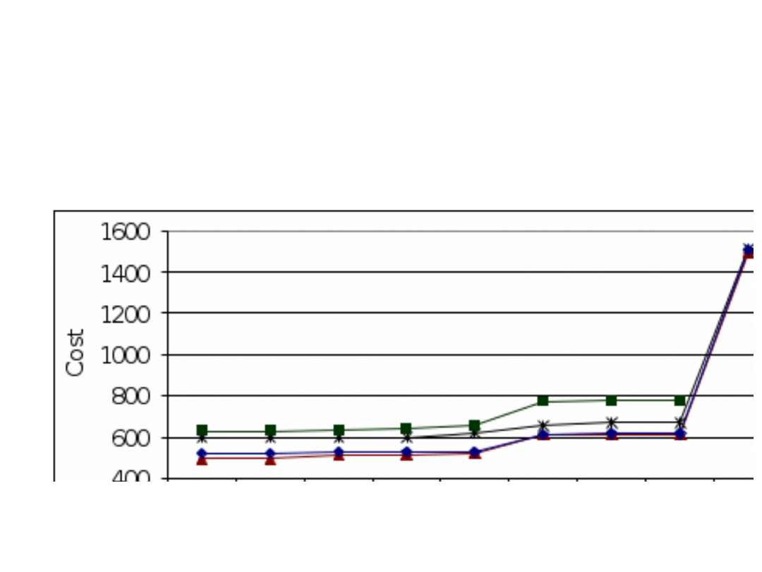
Simulation Approach (3)

• Based on the CSL we develop three strategies

taking into account survivability constraints

– CSL-LD (link disjoint)
– CSL-ND (node disjoint)
– CSL-ID (ISP link disjoint)

• The objective is to create trees covering all

peers - thus, if it is not possible to establish a new
overlay link satisfying survivability constraints, the
uploading peer selects a new downloader without
taking into account disjoint constraints

Results (1)

• Tested networks include randomly generated

5000 peers belonging to 10 ISPs

• 10% of nodes (including roots) are connected to

the Internet by Ethernet links (10Mbps)

• Other nodes use asymmetric links with upload

bandwidth in the range 256-1536 kbps and the
download capacity in the range 2048-12288 kbps

Results (2)

• The overlay link cost is from 3 to 100
• There are two multicast trees, each tree

distributes the data with the rate 256kbps

• We consider two cases: root nodes are located in

separate ISPs, roots are connected to the same

ISP

Algorithms

Strategy

Cost

Common

links

Common

nodes

Common

ISP links

RSL

530511

1.4

356.2

45.0

CSL

221415

723.0

652.8

40.6

CSL-LD

219318

0.0

607.4

41.2

CSL-ND

214344

1.3

0.0

39.8

CSL-ID

220787

3.8

286.3

12.2

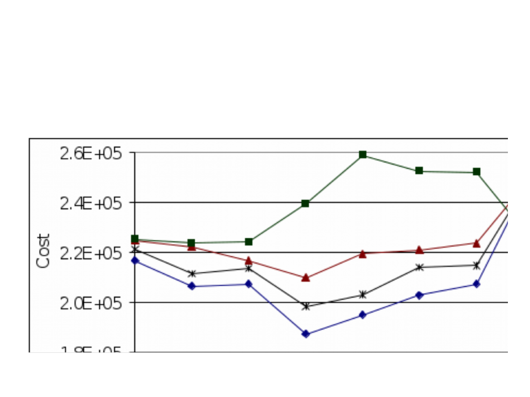
Streaming cost as a function of Ethernet

nodes percentage

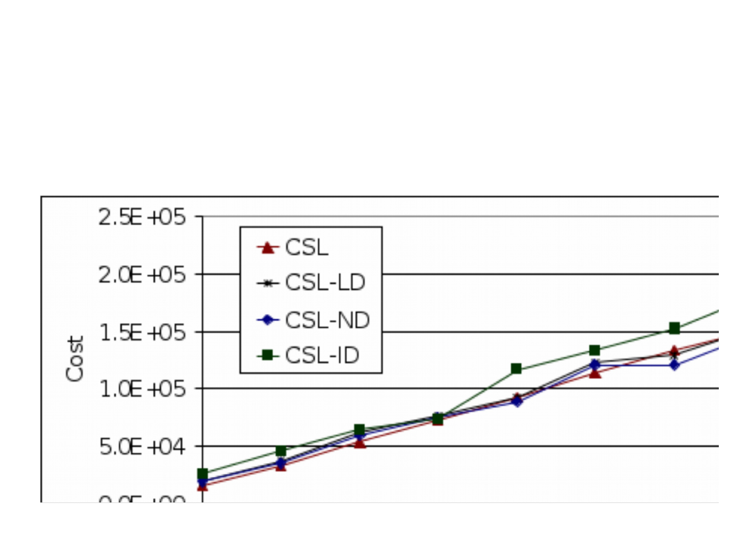
Streaming cost as a function of the number

of nodes

Conclusions

• The requirement to construct failure-disjoint trees

do not influence significantly the objective
functions of cost and throughput

• Consequently, the P2P multicasting system can

be enhanced with additional survivability
criteria without substantial degradation of
the system in terms of the streaming cost and
the system throughput

Lecture Outline

• Introduction
• Failure State Modeling
• Link Protection
• Path Protection
• Restoration
• Survivable P2P Multicasting

• Concluding Remarks

Concluding Remarks

• Survivable networks has been gaining much

attention in recent years due to the growing

importance of computer networks

• Optimization of survivable networks (including flow

and capacity assignment) are more complex than

corresponding classical problems

• However, the same methods as in classical

problems (e.g., Simplex, branch and bound,

Lagrangean relaxation, evolutionary algorithms, etc.)

can be applied to survivable networks optimization

Further Reading

• M. Pióro, D. Medhi, Routing, Flow, and Capacity Design in

Communication and Computer Networks, Morgan Kaufman Publishers

2004

• W. Grover, Mesh-based Survivable Networks: Options and Strategies for

Optical, MPLS, SONET and ATM Networking, Prentice Hall PTR, Upper

Saddle River, New Jersey, 2004

• J. Vasseur, M. Pickavet, P. Demeester, Network Recovery, Protection and

Restoration of Optical, SONET-SDH, IP, and MPLS, Elsevier, 2004

• K. Walkowiak, A New Method of Primary Routes Selection for Local

Restoration, Lecture Notes in Computer Science, Vol. 3042, Springer

Verlag, 2004, s. 1024-1035

• K. Walkowiak, A New Function for Optimization of Working Paths in

Survivable MPLS Networks, Lecture Notes in Computer Science, Vol.

4263, Springer Verlag, 2006, s. 424-433

• K. Walkowiak, Survivability of P2P Multicasting, Proceedings of the 7th

International Workshop on Design of Reliable Communication Networks

DRCN 2009, pp. 92-99