
22/02/05
C.Barbieri Elementi_AA_2004
_05 Sesta settimana
1
Elementi di Astronomia e
Astrofisica per il Corso di
Ingegneria Aerospaziale
VI settimana
L'Atmosfera terrestre
Un esercizio di meccanica celeste
(in English)
22/02/05
C.Barbieri Elementi_AA_2004
_05 Sesta settimana
2
The terrestrial
atmosphere - 1
This chapter is devoted to the examination of the influence of
the Earth’s atmosphere on the apparent coordinates of the
stars and on the shape of their images; the discussion will be
limited essentially to the visual band. The discussion of the
effects
of
the
atmosphere
on
photometry
and
spectrophotometry are deferred to a later chapter.
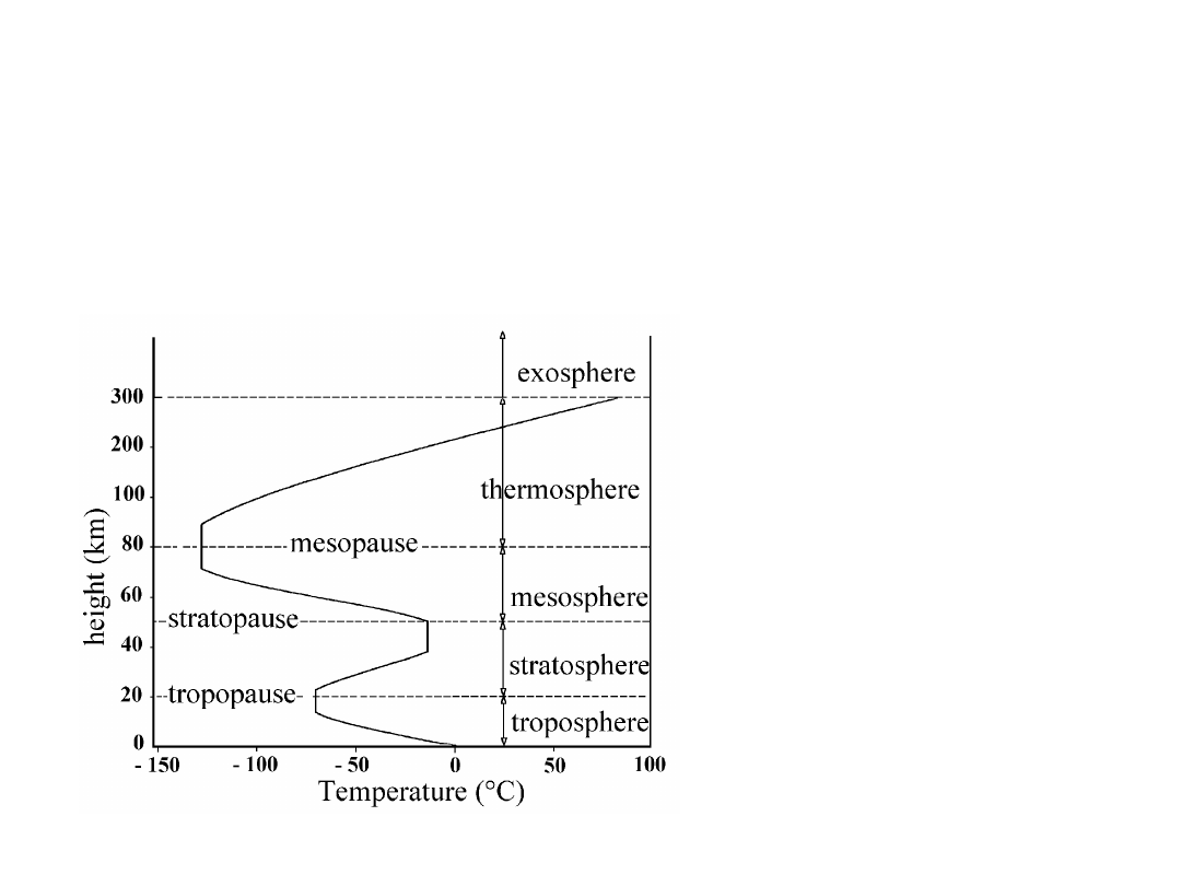
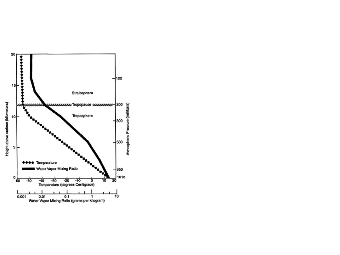
The figure gives a
schematic
representation
of
the
vertical
structure
of
the
atmosphere;
the
visual band is mostly
affected by what
happens
in
the
troposphere
,
namely in
the first
15 km or so of
height, where some
90% of the total
mass
of
the
atmosphere
is
contained.
22/02/05
C.Barbieri Elementi_AA_2004
_05 Sesta settimana
3
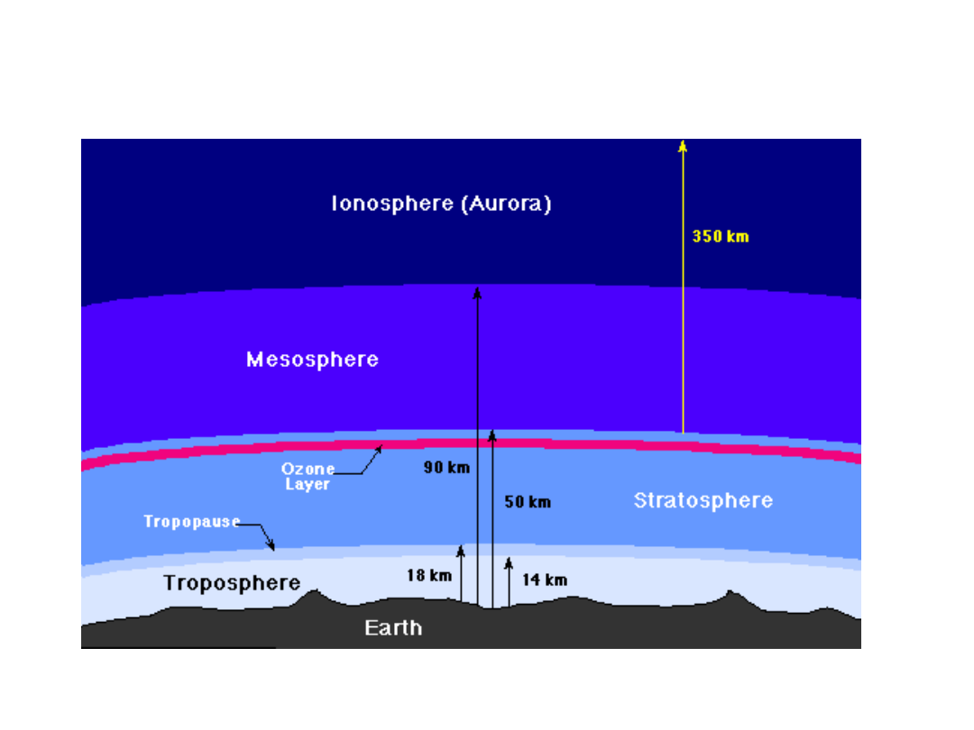
The terrestrial
atmosphere -2
Na Layer
22/02/05
C.Barbieri Elementi_AA_2004
_05 Sesta settimana
4
The terrestrial
atmosphere
- 3
The temperature profile in the troposphere is actually more
complicated than shown in the Figure. The height of the
tropopause (a layer of almost constant temperature) from the
ground ranges from 8 km at high latitudes to 18 km above the
equator; it is also highest in summer and lowest in winter. The
average temperature gradient is approximately –6 C/km, but
often, above a critical layer situated in the first few km,
the
temperature gradient is inverted
, with beneficial effects on
astronomical observations, thanks to the intrinsic stability of
all layers with temperature inversion (such as the
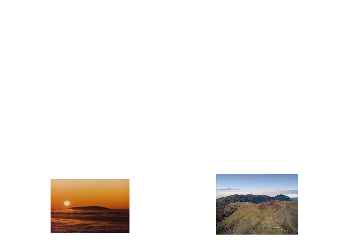
stratosphere and the thermosphere), essentially because
convection cannot develop. This is the case for instance of the
Observatory of the Roque de los Muchachos (Canary Islands,
height 2400 m a.s.l.), where the inversion layer is usually few
hundred meters below the telescopes at the top of the
mountain.

22/02/05
C.Barbieri Elementi_AA_2004
_05 Sesta settimana
5
Chemical composition and
structure
The chemical composition of the troposphere is mostly
molecular
Nitrogen
N
2
and
molecular
Oxygen
O
2
(approximately 3:4 and 1:4 respectively), with traces of the
noble gas
Argon
and of
water vapor
(the water vapor
concentration may be as high as 3% at the equator, and
decreases toward the poles).
Above the tropopause, at higher heights in the
stratosphere
,
the temperature raises considerably thanks to the solar UV
absorption by the Ozone (
O
3
) molecule with the process:
UV photon
+
O
3
=
O
2
+O+
heat
.
The
mesosphere
ranges from 50 to 80 km; in this region,
concentrations of
O
3
and
H
2
O
vapor
are negligible, hence the
temperature is lower than in the stratosphere. The chemical
composition of the air becomes strongly height-dependent, with
heavier gases stratified in the lower layers. In this region,
meteors and spacecraft entering the atmosphere start to warm
up.
22/02/05
C.Barbieri Elementi_AA_2004
_05 Sesta settimana
6
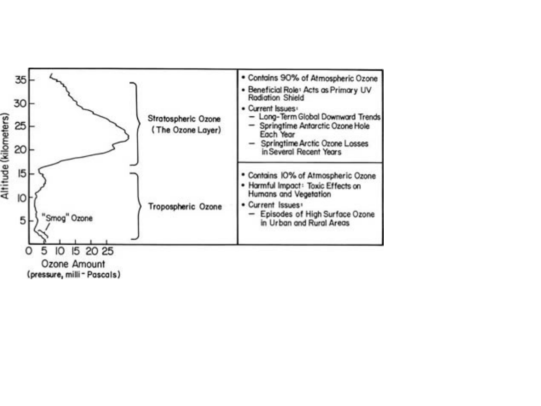
The ozone O
3
Most atmospheric ozone is concentrated in a layer in the
stratosphere, about 15-30 kilometers above the Earth's
surface. Even this small amount of ozone plays a key role in
the atmosphere, absorbing the
UVB
portion of the radiation
from the sun, preventing it from reaching the planet's surface.
O
3
is a molecule
containing 3 O
atoms.
It is blue
in color and has a
strong odor.
Normal molecular
O
2
, has 2 oxygen
atoms and is
colorless and
odorless. Ozone
is much less
common than
normal oxygen.
Out of each 10
million air
molecules, about
2 million are
normal oxygen,
but only 3 are
ozone.

22/02/05
C.Barbieri Elementi_AA_2004
_05 Sesta settimana
7
Water vapor nomenclature
- 1
Water vapor
is water in the gaseous phase.
The actual amount is the
concentration
of water vapor in the
air, the
relative concentration
is the ratio between the actual
amount to the amount that would saturate the air. Air is said
to be saturated when it contains the maximum possible
amount of water vapor without bringing on condensation. At
that point, the rate at which water molecules enter the air by
evaporation exactly balances the rate at which they leave by
condensation.
The partial pressure of a given sample of moist air that is
attributable to the water vapor is called the vapor pressure.
The vapor pressure necessary to saturate the air is the
saturation vapor pressure.
Its value depends only on the
temperature of the air
. (The Clausius-Clapeyron equation
gives the saturation vapor pressure over a flat surface of pure
water as a function of temperature.) Saturation vapor
pressure increases rapidly with temperature: the value at
32°C is about double the value at 21°C. The saturation vapor
pressure over a curved surface, such as a cloud droplet, is
greater than that over a flat surface, and the saturation vapor
pressure over pure water is greater than that over water with
a dissolved solute.

22/02/05
C.Barbieri Elementi_AA_2004
_05 Sesta settimana
8
Water vapor nomenclature
- 2
Relative humidity
is the ratio of the actual vapor pressure to
the saturation vapor pressure at the air temperature, expressed
as a percentage. Because of the temperature dependence of the
saturation vapor pressure, for a given value of relative humidity,
warm air has more water vapor than cooler air. The d
ew point
temperature
is the temperature the air would have if it were
cooled, at constant pressure and water vapor content, until
saturation (or condensation) occurred. The difference between
the actual temperature and the dew point is called the dew
point depression.
The wet-bulb temperature is the temperature an air parcel
would have if it were cooled to saturation at constant pressure
by evaporating water into the parcel. (The term comes from the
operation of a psychrometer, a widely used instrument for
measuring humidity, in which a pair of thermometers, one of
which has a wetted piece of cotton on the bulb, is ventilated. The
difference between the temperatures of the two thermometers is
a measure of the humidity.) The wet-bulb temperature is the
lowest air temperature that can be achieved by evaporation. At
saturation, the wet-bulb, dew point, and air temperatures are all
equal; otherwise the dew point temperature is less than the wet-
bulb temperature, which is less than the air temperature.
22/02/05
C.Barbieri Elementi_AA_2004
_05 Sesta settimana
9
Water Vapor Mixing ratio
Specific humidity
is the ratio of the
mass of water vapor in a sample to the
total mass, including both the dry air
and the water vapor. The
mixing ratio
is the ratio of the mass of water vapor to
the mass of only the dry air in the
sample. As ratios of masses, both
specific humidity and mixing ratio are
dimensionless numbers. However,
because atmospheric concentrations of
water vapor tend to be
at most only a
few percent of the amount of air
(and
usually much lower), they are both often
expressed in units of grams of water
vapor per kilogram of (moist or dry) air.
Absolute humidity is the same as the
water vapor density, defined as the mass
of water vapor divided by the volume of
associated moist air and generally
expressed in grams per cubic meter. The
term is not much in use now.
22/02/05
C.Barbieri Elementi_AA_2004
_05 Sesta settimana
10
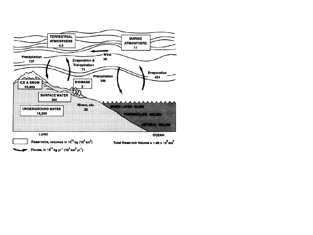
Water reservoir
Water
vapor
is
constantly
cycling
through
the
atmosphere,
evaporating from the
surface, condensing to
form clouds blown by
the
winds,
and
subsequently
returning to the Earth
as precipitation. Heat
from the Sun is used
to evaporate water,
and this heat is put
into the air when the
water condenses into
clouds
and
precipitates.
This
evaporation
-
condensation cycle is
an
important
mechanism
for
transferring
heat
energy
from
the
Earth's surface to its
atmosphere and in
moving heat around
the Earth.
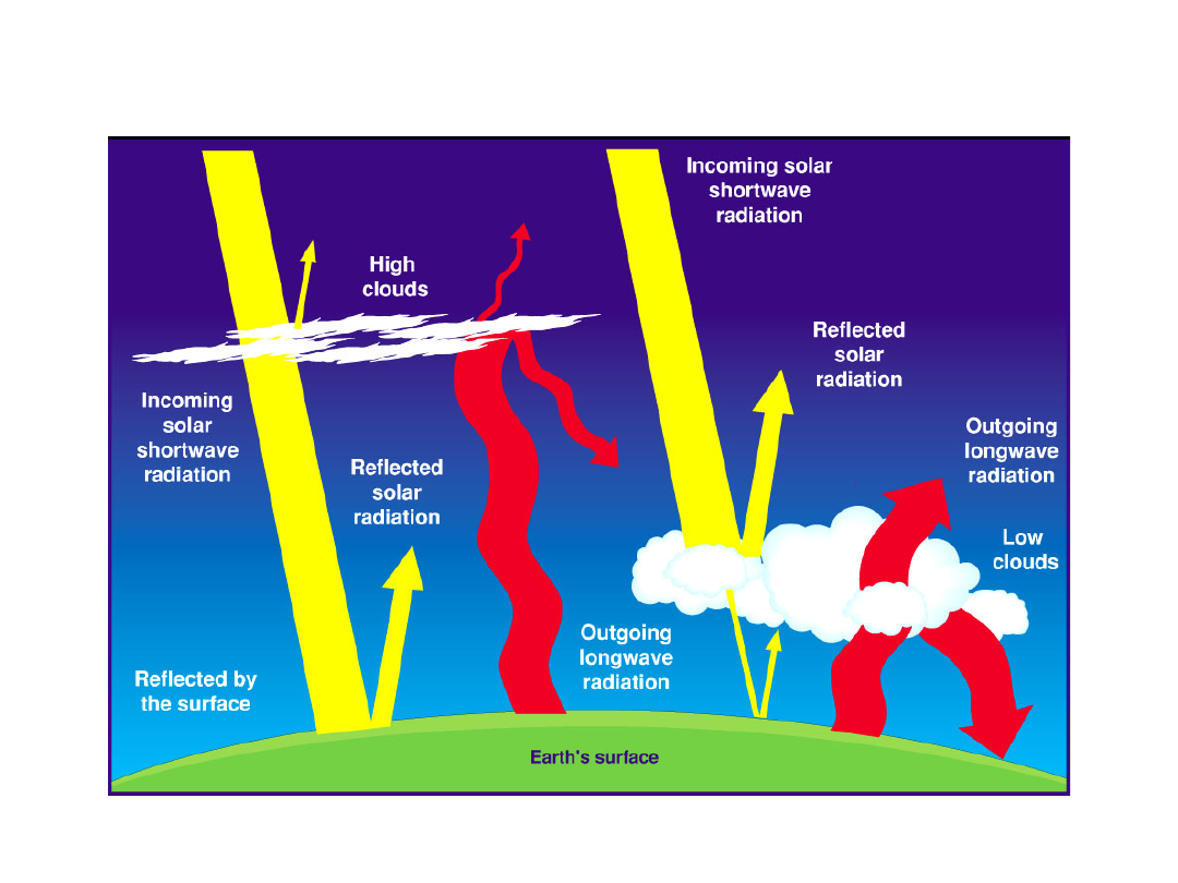
Water vapor is the most abundant of the
greenhouse gases in the atmosphere and the
most important in establishing the Earth's
climate. Greenhouse gases allow much of the
Sun's shortwave radiation to pass through
them but absorb the infrared radiation
emitted by the Earth's surface. Without water
vapor and other greenhouse gases in the air,
surface air temperatures would be well below
freezing.
22/02/05
C.Barbieri Elementi_AA_2004
_05 Sesta settimana
11
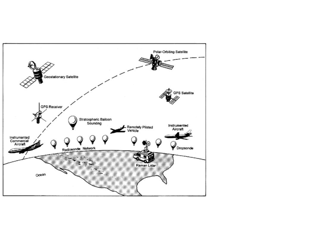
Aerospace
devices
A multitude of
systems exist for
observing water
vapor on a global
scale and at high
altitudes,
supplementing the
instruments on the
ground, that measure
in special sites and at
ground level. Each
has different
characteristics and
advantages. To date,
most large-scale
water vapor
climatological studies
have relied on
analysis of
radiosonde data,
which have good
resolution in the
lower troposphere in
populated regions but
are of limited value at
high altitude and are
lacking over remote
oceanic regions.
22/02/05
C.Barbieri Elementi_AA_2004
_05 Sesta settimana
12
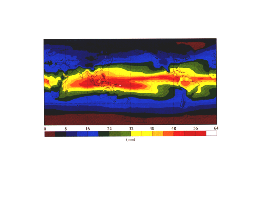
The Water Vapor content
in 1992
NASA Water Vapor Project (NVAP) Total Column Water
Vapor 1992
The mean distribution of precipitable water, or total atmospheric
water vapor above the Earth's surface, for 1992. This depiction
includes data from both satellite and radiosonde observations.
22/02/05
C.Barbieri Elementi_AA_2004
_05 Sesta settimana
13
Cloud effects on Earth
Radiation

22/02/05
C.Barbieri Elementi_AA_2004
_05 Sesta settimana
14
The outer layers
Following the smooth decrease in the mesosphere, the
temperature raises again in the
thermosphere
, because the
solar UV and X-rays, and the energetic electrons from the
magnetosphere can partly ionize the very thin gases of the
thermosphere.
The weakly ionized region which conducts electricity, and
reflects radio frequencies below about 30 MHz is called
ionosphere
; it is divided into the regions
D
(60-90 km),
E
(90-140 km), and
F
(140-1000 km), based on features in the
electron density profile.
Finally, above 1000 km, the gas composition is dominated by
atomic Hydrogen escaping the Earth’s gravity, which is seen
by satellites as a bright
geocorona
in the resonance line
Ly-
at
= 1216 Å.
22/02/05
C.Barbieri Elementi_AA_2004
_05 Sesta settimana
15
Refraction Index
As is well known, the light propagates in a straight line in any
medium of constant refraction index
n
, with a phase velocity
v
given by
1/2
v
/
1/( )
c n
em
=
=
where
is the dielectric constant and
the magnetic
permeability of the medium. All these quantities are
wavelength dependent. The group velocity
u
is instead:
v
dv/d
u
l
l
= -
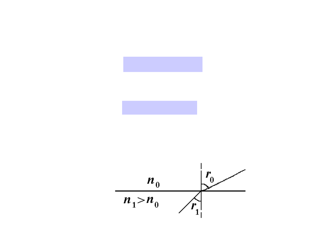
At the separation surface between two media of different
refraction index (say vacuum/air), the ray changes direction,
so that the observer immersed in the second medium sees the
light coming from an apparent direction different from the
‘true’ one (see Figure):

22/02/05
C.Barbieri Elementi_AA_2004
_05 Sesta settimana
16
The atmospheric
refraction - 1
Suppose that the atmosphere can be treated as a succession of
parallel planes (hypothesis of
plane-parallel stratification
),
by virtue of its small vertical extension with respect to the
Earth’s radius. According to
Snell’s laws
, when the ray
coming from the region of index of refraction
n
0
encounters the
separation surface with a medium of refraction index
n
1
>
n
0
,
part of the energy will be reflected to the left, on the same
hemi-space with the same angle
r
0
with respect to the normal.
This part will not be considered here, it only implies a dimming
of the source. The remaining fraction will be
refracted
, in the
same plane as the incident ray, to an angle
r
1
<
r
0
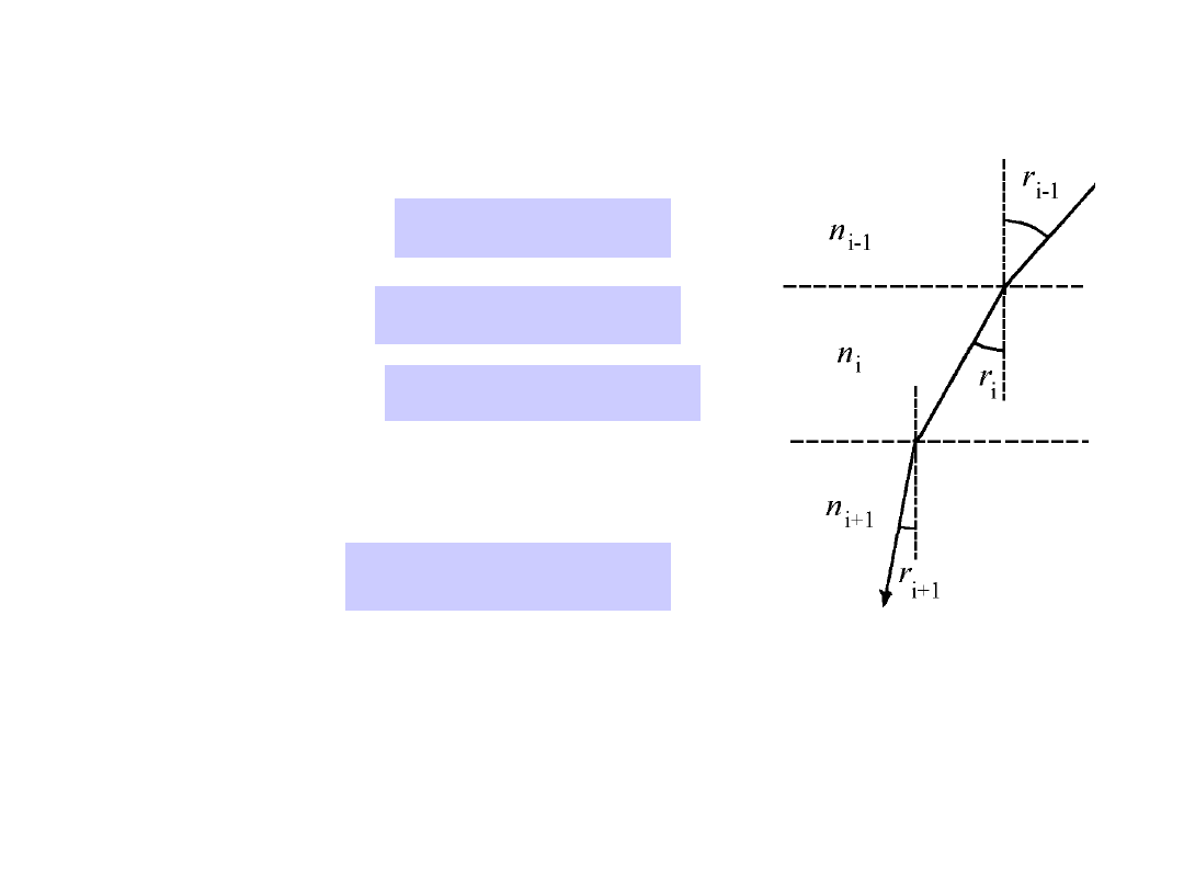
. Indeed, in a
clear atmosphere without clouds, no sharp air-vacuum
separation surface exists, the refraction index gradually
increases from 1 to a final value
n
f
near the ground, with
typical scale lengths much greater than the wavelength of light
(as already said, we limit our considerations to the visual
band), so that the continuously varying direction can be
considered as a series of finite steps in the plane passing
through the vertical and the direction to the star.
22/02/05
C.Barbieri Elementi_AA_2004
_05 Sesta settimana
17
The atmospheric
refraction - 2
0
0
1
1
sin
sin
n
r
n
r
=
1 1
1
sin
sin
i
i
i
n
r n
r
+
+
=
1
1
sin
sin
ff
ff
n
r
n
r
-
-
=
where
n
i+1
>
n
i
, and
r
i+1
<
r
i
. By equating each term:
0
0
sin
sin
ff
n
r
n
r
=
Therefore: in a plane-parallel atmosphere the total angular
deviation only depends on the refraction index close to the
ground, independent of the exact law with which it varies
along the path.
By following each refraction in cascade we have:
22/02/05
C.Barbieri Elementi_AA_2004
_05 Sesta settimana
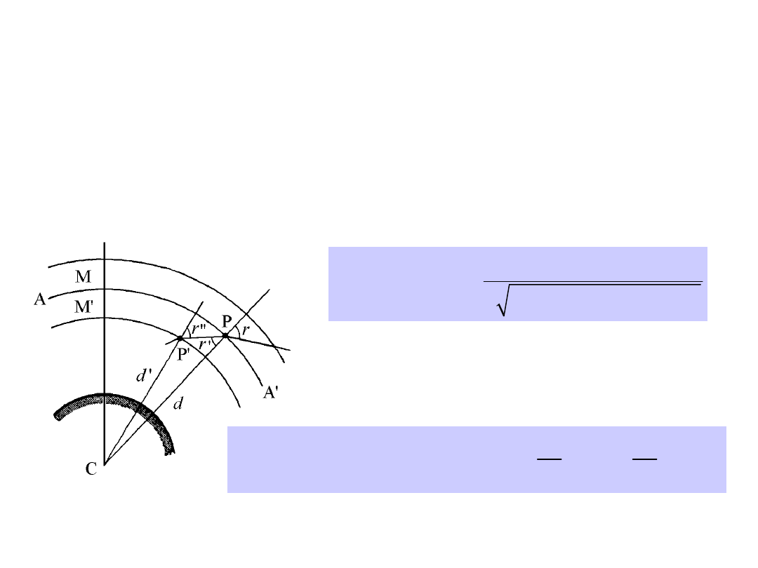
18
The atmospheric
refraction - 3
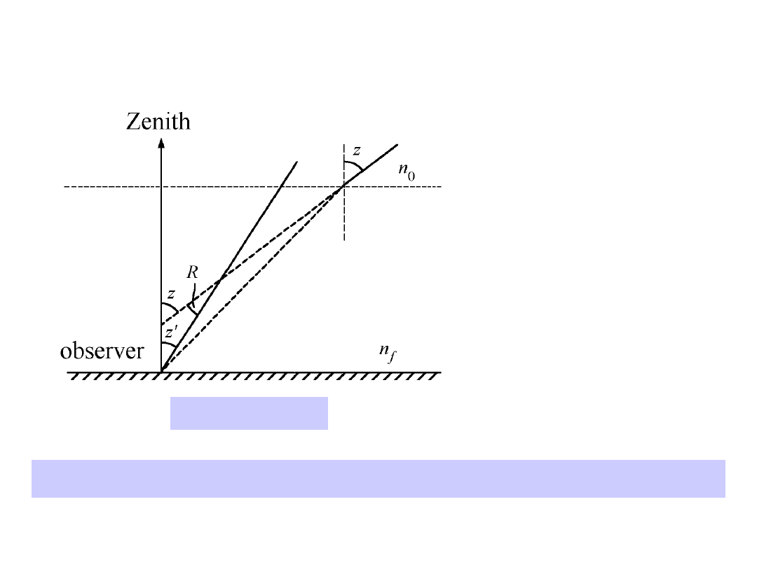
By virtue
of
The net effect is as
shown in the figure:
the star is seen in
direction
z’
smaller
than the true direction
z
, namely closer to the
local Zenith, by an
amount
R
which is the
atmospheric
refraction:
z’
=
z
–
R
0
0
sin
sin
ff
n
r
n
r
=
and for small
R
’s (in practice, if
z
< 45°):
sin ' sin
sin( '
) sin 'cos
cos 'sin
sin '
cos '
f
n
z
z
z R
z
R
z
R
z R
z
=
=
+ =
+
�
+

22/02/05
C.Barbieri Elementi_AA_2004
_05 Sesta settimana
19
The atmospheric
refraction - 4
(
1)tan '
f
R
n
z
=
-
In the visual band, for average values of temperature and
pressure (
T
= 273 K,
P
= 760 mm Hg),
n
f
1.00029, so that
in round numbers
R(15°) 16”,
R(45°) 60”
Already for Zenith distances as small as 20°, the refraction is
larger than the annual aberration, and of any of the effects
discussed in previous chapters that alter the apparent
direction of a star.
and finally:
22/02/05
C.Barbieri Elementi_AA_2004
_05 Sesta settimana
20
The atmospheric
refraction - 5
For zenith distances larger than 45°, the path of the ray
inside the atmosphere is so long that the curvature of the
Earth cannot be ignored, and the mathematical treatment
becomes more intricate, even restricting it to successive
refraction in the same plane with
n
decreasing outwards
with continuity.
2
2
2
2
2
1
d
sin '
sin '
f
n
f
f
n
R a n
z
n d n
a
n
z
�
�
= �
� -
�
�
3
3
tan '
tan ' (
1) (1
)tan '
tan '
f
l
l
R A
z B
z
n
z
z
a
a
�
�
�
�
=
+
=
-
-
-
�
�
�
�
After
several
mathematical
steps:
22/02/05
C.Barbieri Elementi_AA_2004
_05 Sesta settimana
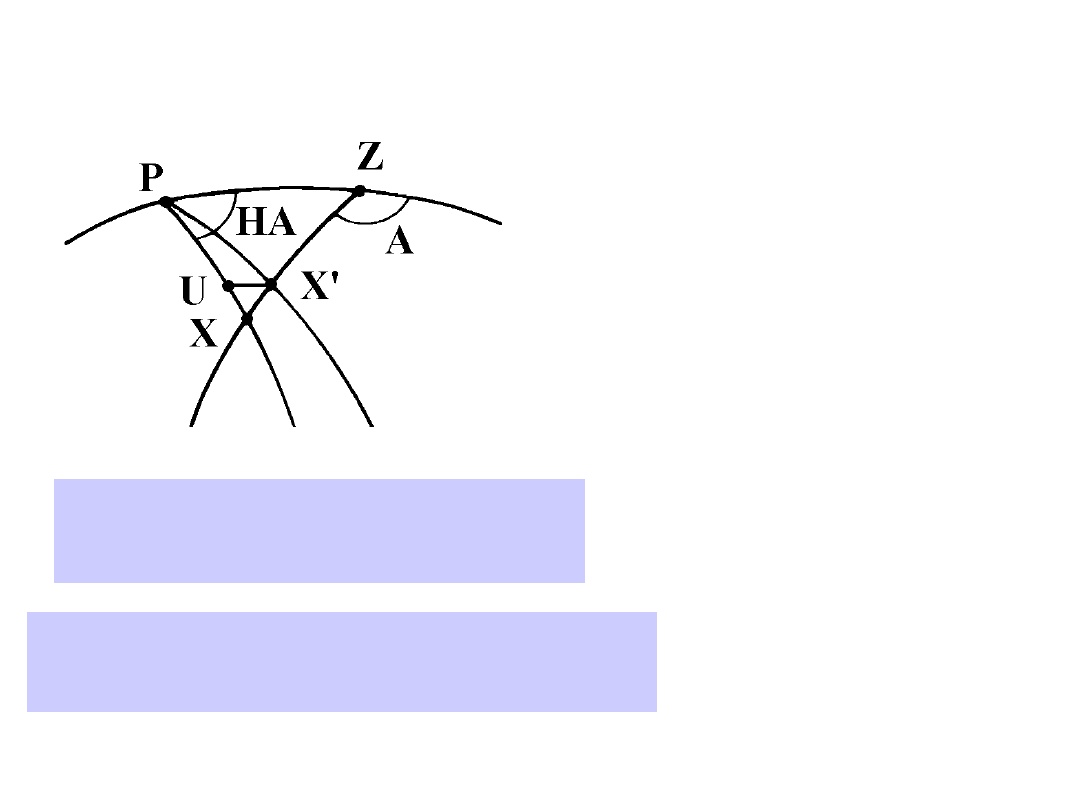
21
Effect of the refraction on the
coordinates
The main effect of refraction is
to move the star closer to the
Zenith in the vertical plane,
thus raising its elevation
h
but
leaving essentially unchanged
its azimuth
A
.
XX’ = R = h
PXX’ = PXZ = q
ZX = z, ZX’ = z’
PX = 90-
XU =
cos
( '
)cos
sin
'
cos
HA
R
q
R
q
d
a a
d
d d d
- D
=
-
=
�
�
D = -
=
�
cos cos
sin cos
cos sin cos
sin sin
cos
sin
sin
cos sin
q
h
h
A
A
h
HA
q
HA
q
d
j
j
d
=
+
=
+
For an object in
meridian,
the
refraction is all in
declination, and in
particular this is
true for the Sun at
true noon.

22/02/05
C.Barbieri Elementi_AA_2004
_05 Sesta settimana
22
Approximate formulae for
refraction
For Zenith distance not greater than approximately 45°, after
several passages we finally get:
2
sec sin
(
1)
cos
tan tan
tan
tan cos
(
1)
cos
tan tan
f
f
HA
n
HA
HA
n
HA
d
a
j
d
j
d
d
j
d
�
D =
-
�
+
�
�
-
�D = -
�
+
�
by means of which formulae we can derive the true (or the
apparent, according to the sign)
topocentric
positions.
Obviously no such correction is necessary for a telescope in
outer Space.
22/02/05
C.Barbieri Elementi_AA_2004
_05 Sesta settimana
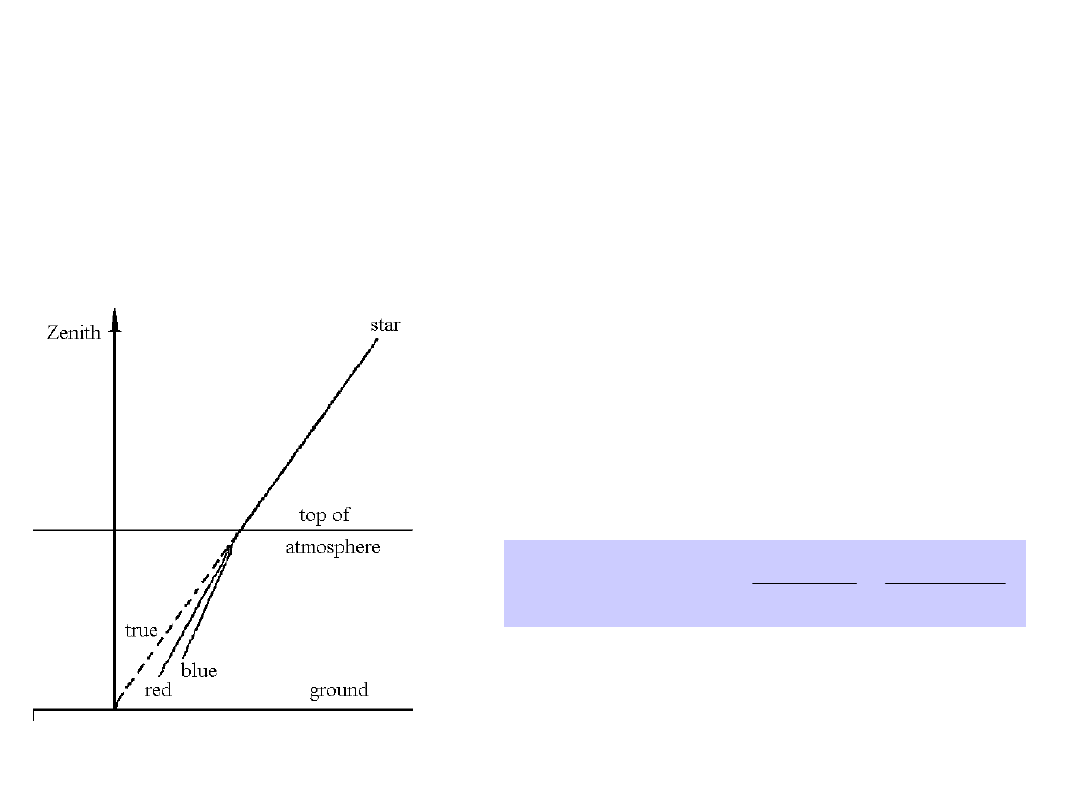
23
The chromatism of the
refraction
The refraction index
n
depends from the wavelength,
diminishing from the blue to the red, and the same will be true
for the refraction angle
R
: the image on the ground of the star
is therefore a succession of monochromatic points aligned
along the vertical circle; the blue ray will be below the red
one, and thus the blue star will appear to the eye above the
red one
The atmosphere behaves therefore
like a prism producing a
short
spectrum in the vertical plane
,
whose length increases with the
zenith distance, reaching several
arc seconds at low elevations. The
relationships
n(
)
can
be
expressed
by
the
so-called
Cauchy’s formula:
2
4
0.00566 0.000047
( ) 0.00028 1
n l
l
l
�
�
=
+
+
�
�
�
�
(
in micrometers), corresponding to a
variation of about 2% over the visible
range, namely to about
1”.2 at 45°.
22/02/05
C.Barbieri Elementi_AA_2004
_05 Sesta settimana
24
Density - temperature
relationship
Once we have fixed
, the refraction index
n
depends from the
density
according to Gladstone-Dale’s law:
1
n
kr
- =
and with the hypothesis of a perfect gas of pressure
P
,
temperature
T
and molecular weight
:
R
P
T
m
r =
(where
R
is now the gas universal
constant)
1
'
P
n
k
T
- =
0
0
0
1
1
T
n
P
n
P T
-
=
-
6
1 78.7 10
P
n
T
-
- �
�
( /760)
60".4
tan
( / 273)
P
R
z
T
�
(
P
in mm Hg,
T
in K)
22/02/05
C.Barbieri Elementi_AA_2004
_05 Sesta settimana
25
Vertical gradients of
temperature
Calling
H
the height over the ground,
we have:
1
d
'
d
d
P
n k
P
T
T
T
�
�
=
-
�
�
�
�
2
2
d
1 d
d
d
d
'
'
d
d
d
d
d
n
P
P T
P T P
T
k
k
H
T H T
H
T
P H
H
�
�
�
�
=
-
=
-
�
�
�
�
�
�
�
�
The variation of pressure with the height is equal to the weight
of the air in the elementary volume having unitary base and
height
dH
,
d
d
P
g H
r
=-
so
that:
2
d
d
'
d
R
d
n
P
g
T
k
H
T
H
m
m
�
�
-
=
-
�
�
�
�
where the constant
g/R
equals approximately 3.4 K/km, and is
called
adiabatic lapse
.
Hence the conclusion that the variations of the refraction index
depend from the vertical gradients of the temperature. A
practical consequence is that all effort must be made to control
and minimize those gradients over the accessible volume of the
telescope enclosure.

23/02/05
C.Barbieri Elementi_AA_2004
_05 Sesta settimana
26
Turbulence, Scintillation,
Seeing
The Earth's atmosphere is turbulent and variations in the
index of refraction cause the plane wavefront from distant
objects to be
distorted
. This distortion introduces
amplitude
variations
,
positional shifts
and
image degradation
.
This causes two astronomical effects:
•scintillation
, which is amplitude variations, which typically
varies over scales of few cm: generally very small for large
aperture telescopes
•seeing
: positional changes and image quality changes. The
effect of seeing depends on aperture size: for small apertures,
one sees a diffraction pattern moving around, while for large
apertures, one sees
a set of diffraction patterns
(
speckles
)
moving around on scale of ~1 arcsec.
These observations imply:
• wavefronts are flat on scales of small apertures
• instantaneous slopes vary by ~ 1 arcsec.
The typical time scales are few
milliseconds
and up.
The effect of seeing can be derived from theories of
atmospheric turbulence, worked out originally by
Kolmogorov, Tatarski, Fried.
23/02/05
C.Barbieri Elementi_AA_2004
_05 Sesta settimana
27
Structure function
The structure of the refraction index
n
in a turbulent field can
be described statistically by a
structure function
:
2
( )
(
)
( )
n
D x
n r x n r
=� + -
�
where
x
is separation of points,
r
is position. Kolmogorov
turbulence gives:
2 2
1
( )
3
n
n
D x
C x
=
where
C
n
is the refractive index structure constan
t. From this,
one can derive the
phase structure function
at the
telescope aperture:
5/2
0
6.88
x
D
r
f
=
where the coherence length
r
0
(also known as the Fried
parameter) is:
3/5
6/5
3/5
2
0
0
0.185
cos
d
r
z C h
l
-
�
�
=
�
�
�
where
z
is zenith angle,
is
wavelength. Using optics theory,
one can convert D
into an
image shape.

23/02/05
C.Barbieri Elementi_AA_2004
_05 Sesta settimana
28
The Fried parameter
Notice that
r
0
increases with
6/5
=
1. 2
.
Physically, the image size
d
from seeing is (roughly) inversely
proportional to
r
0
0
/
d
r
l
�
as compared with the image size from a diffraction-limited
telescope of aperture
D
:
/
d
D
l
�
Seeing dominates when
r
0
<
D
; a larger
r
0
means better
seeing. Seeing is more important than diffraction at shorter
wavelengths, diffraction more important at longer wavelengths;
effect of diffraction and seeing cross over in the IR (at 5
microns for 4m); the crossover falls at a shorter wavelength for
smaller telescope or better seeing. Fried’s parameter
r
0
varies
from site to site and also in time. At most sites, there seems to
be three regimes called:
surface layer
(wind-surface interactions and manmade seeing),
planetary boundary layer
( influenced by diurnal heating),
free atmosphere
(10 km is tropopause: high wind shears)
23/02/05
C.Barbieri Elementi_AA_2004
_05 Sesta settimana
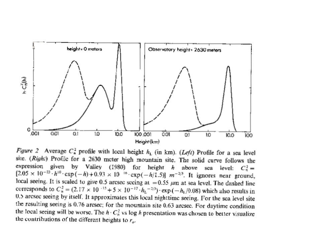
29
An example of
C
n
2
A typical
site has
r
0
10
cm
at 5000Å ,
namely a
seeing of
1". On
rare
occasions,
in the
best sites,
the seeing
can be as
low as
0".3.

23/02/05
C.Barbieri Elementi_AA_2004
_05 Sesta settimana
30
The isoplanatic angle
We also have to consider the coherence of the same
turbulence pattern over the sky: coherence angle call the
isoplanatic angle
:
0
0.314 /
r H
q �
where
H
is the average distance of the seeing layer:
For
r
0
10 cm,
H
= 5000 m ,
1.3 arcsec.
In the infrared
r
0
70 cm,
H
= 5000 m ,
9 arcsec.
Note however, that the ``isoplanatic patch for image motion"
(not wavefront) is 0.3
D/H
. For
D
= 4m,
H
= 5000 m,
kin
50 arcsec.
-
Another useful parameter is the correlation time
0
, which is approximately the dimension of the typical air
bubble divided by the velocity of the wind. As
r
0
,
also
0
increases with
6/5
.
23/02/05
C.Barbieri Elementi_AA_2004
_05 Sesta settimana
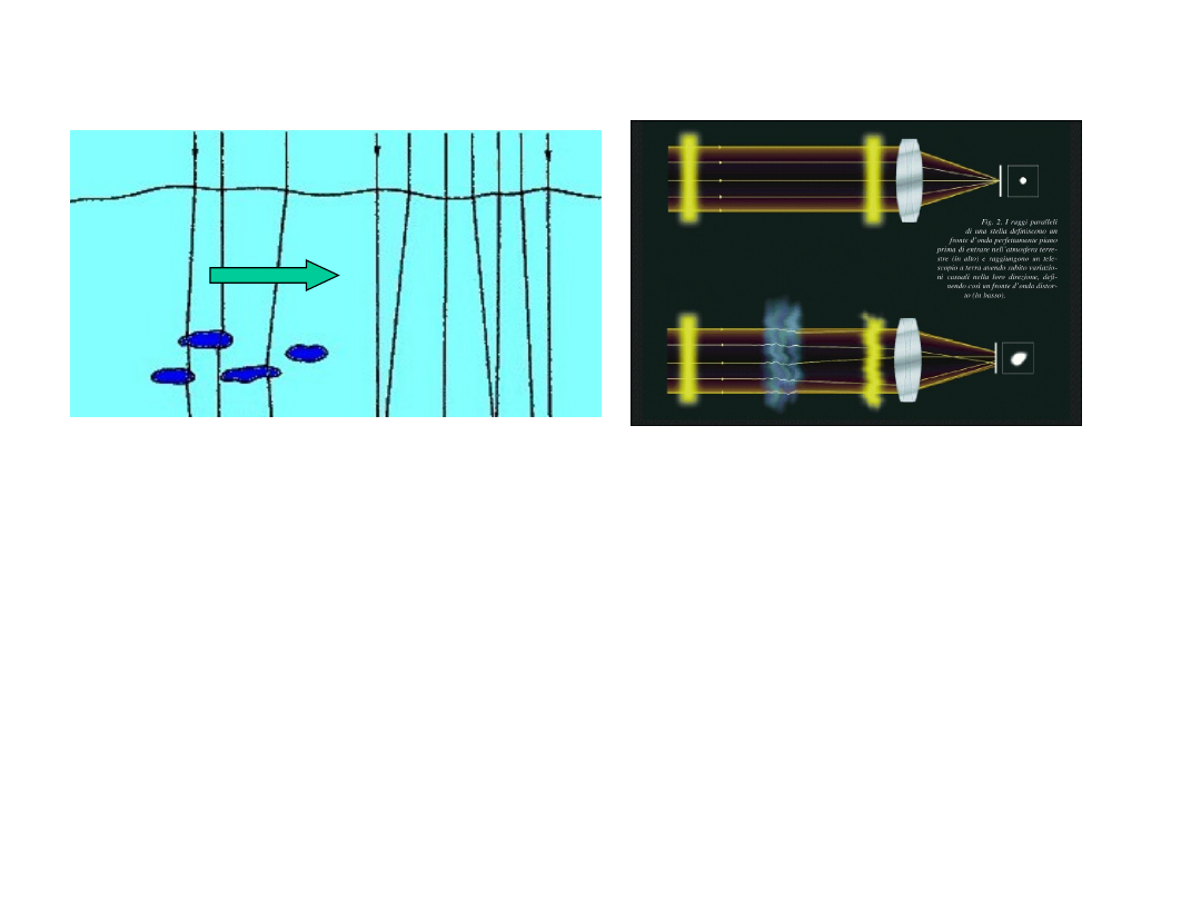
31
The seeing
Bubbles of air having slightly different temperatures, and
therefore slightly different refractive indexes, are carried by the
wind across the aperture of the telescope.
The Fried parameter
r
0
can be used to simplify the description
of a very complex rapidly varying medium, namely the typical
size of the bubble. Values vary from few centimeters (a poor site)
to some 30 cm (a very good site).
r
0
can be understood
also as
the effective
diameter
of the
diffraction limited telescope in that site (with respect to the
angular resolution).
23/02/05
C.Barbieri Elementi_AA_2004
_05 Sesta settimana
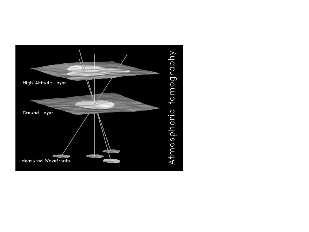
32
Representation of the
seeing
There are two main
components of the
seeing:
•one coming from high
altitudes (choice of
site)
•one due to ground
layers (it can be
actively controlled by
shape of dome and
proper thermalisation
of structure)
• The spectral power of
the air turbulence is
appreciable over a large
interval of frequencies ,
say 1 to 1000 Hz, with a
1/f distribution.
The angles are exaggerated, actually AdOpt correction can be
made over small fields of view. Another useful parameter is the
maximum angle over which fluctuations are coherent
(isoplanatic angle). Both Fried’s parameter and isoplanatic
angle improve with increasing wavelength, the correction is
better in the IR than in the Visible.
23/02/05
C.Barbieri Elementi_AA_2004
_05 Sesta settimana
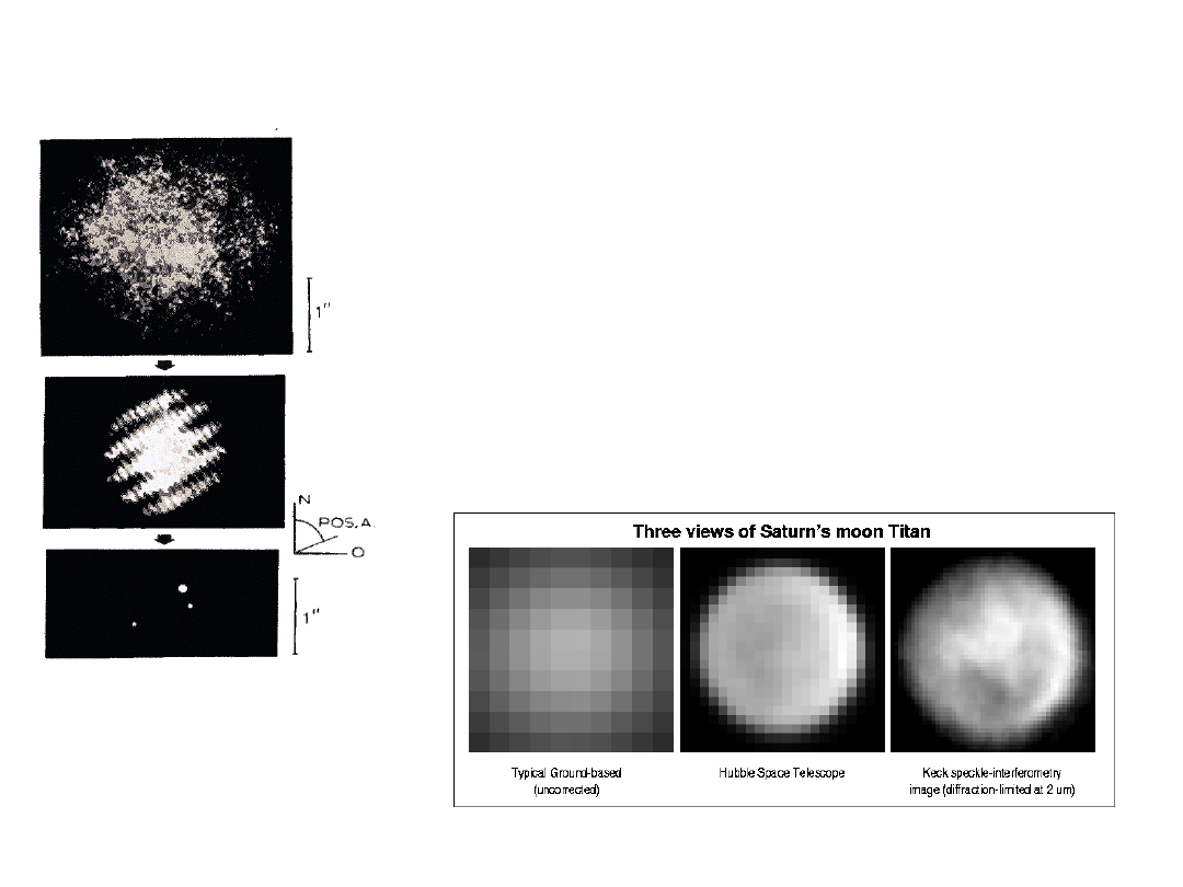
33
A first remedy: Speckle
Interferometry
• a very large number of short duration
exposures are taken with very long focal length
(say 100m) and narrow bandwidth (say 1 nm);
in each exposure the seeing is frozen, each
speckle represents the diffraction figure of the
aperture
• Fourier Transforms allow the reconstruction of
the true image;
• The technique works well for simple structures
(e.g. double or multiple stars, disks).
Obtained
with the
Asiago 1.8
cm telescope
23/02/05
C.Barbieri Elementi_AA_2004
_05 Sesta settimana
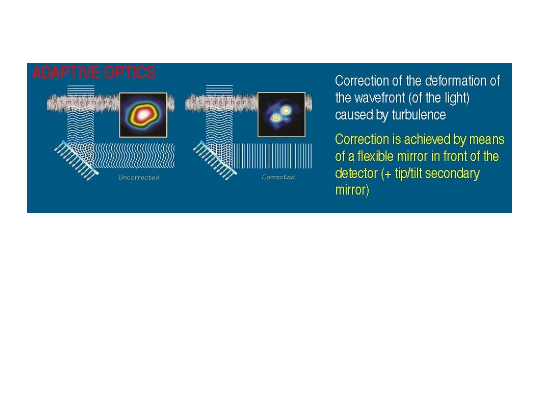
34
A better remedy: Adaptive
Optics
The fairly complex techniques that are nowadays
implemented on the largest telescopes to contrast the
seeing are known collectively as
Adaptive Optics
devices.
• A suitable reference wavefront is also necessary
.
Suitably bright stars are rare.
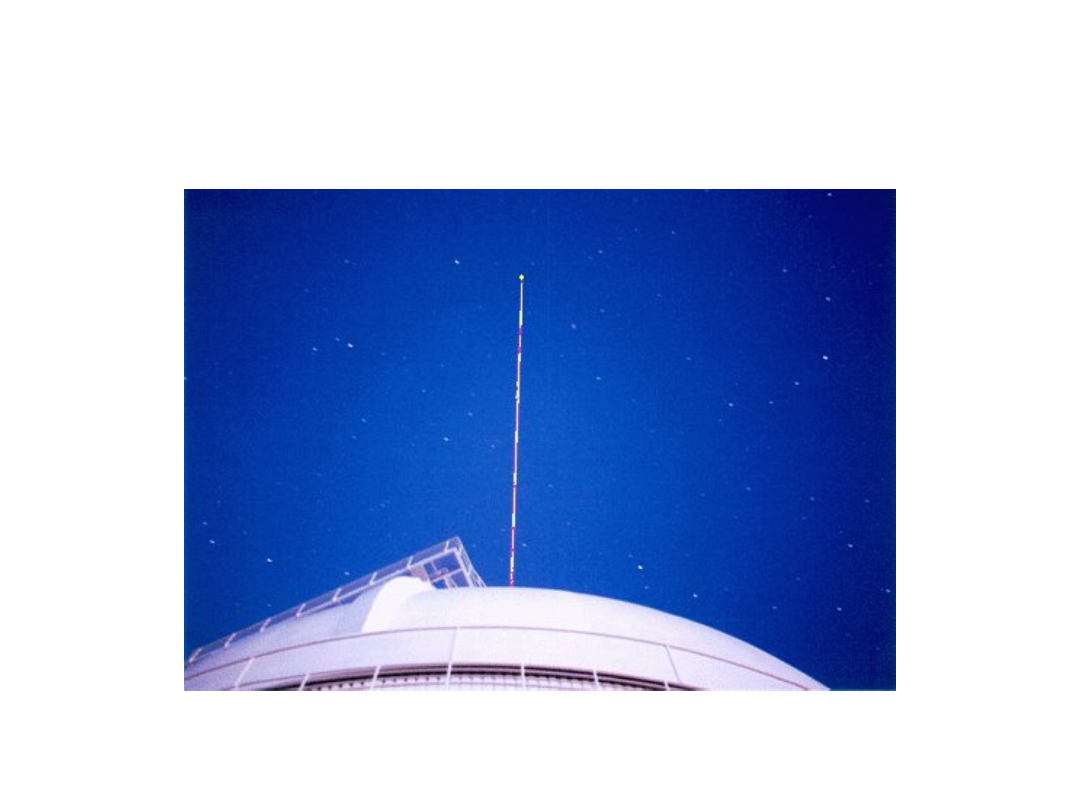
•An artificial
laser star
is a possible solution.
23/02/05
C.Barbieri Elementi_AA_2004
_05 Sesta settimana
35
The artificial laser star
23/02/05
C.Barbieri Elementi_AA_2004
_05 Sesta settimana
36
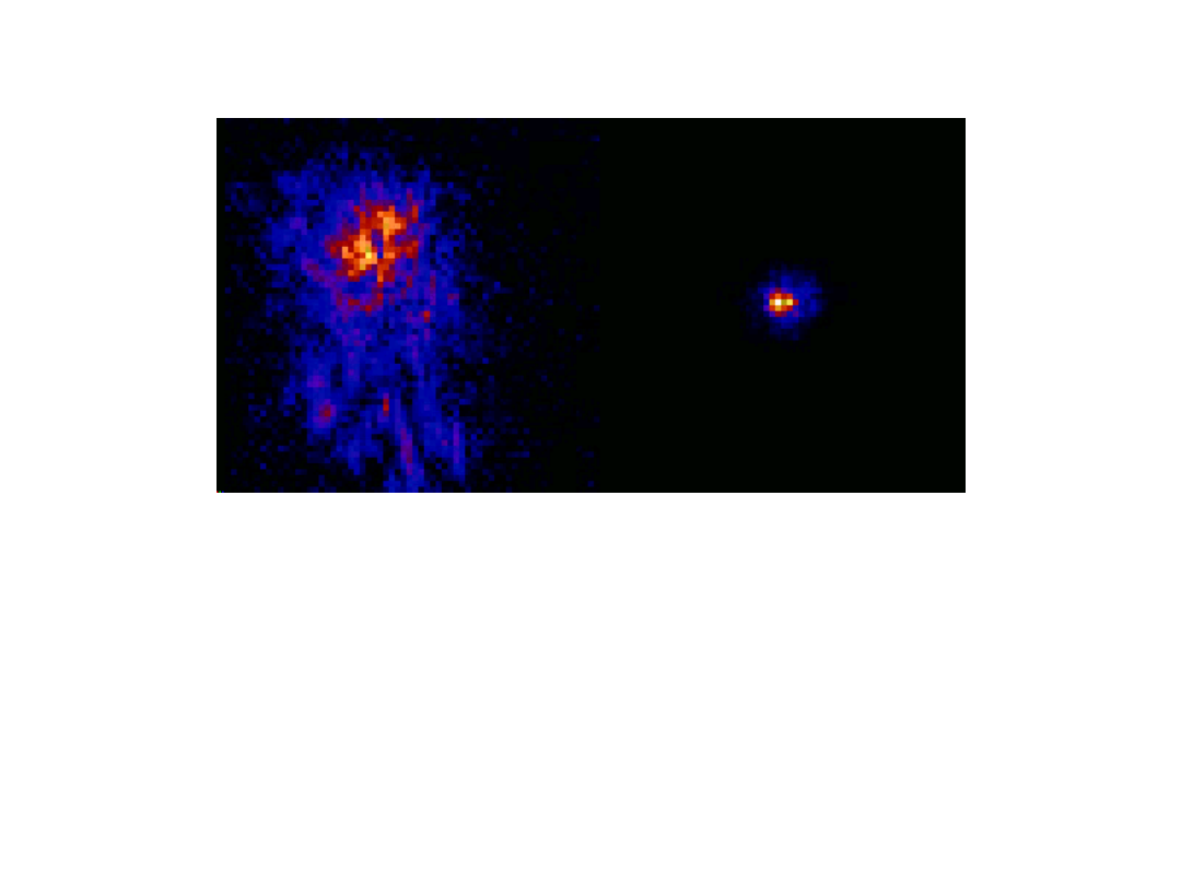
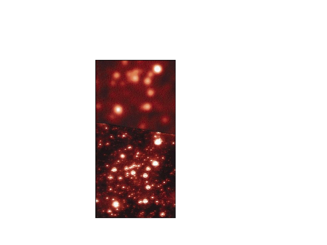
Before and after AdOpt
If one ‘freezes’ the image with short exposure times (say less
than 0.01 sec) and a narrow filter, the seeing image breaks up in
large number of ‘speckles’, each having dimension of the order
of the diffraction figure of the telescope.
The number of speckles is of the order of :
(seeing diameter/diffraction figure)
2
23/02/05
C.Barbieri Elementi_AA_2004
_05 Sesta settimana
37
The Galactic Center with the
Keck AdOpt
Without AdOpt
With AdOpt
23/02/05
C.Barbieri Elementi_AA_2004
_05 Sesta settimana
38
Quality of the image -1
The quality of an image can be described in many different
ways. The overall shape of the distribution of light from a point
source is specified by the
point spread function (PSF)
.
Diffraction gives a basic limit to the quality of the PSF, but any
aberrations or image motion add to structure/broadening of
the PSF.
Another way of describing the quality of an image is to specify
it's modulation transfer function (MTF). The MTF and PSF are
a Fourier transform pair. Turbulence theory gives:
5/3
3.44( / )
MTF
a
v
e
l
t
-
=
where
is the spatial frequency. Note that a Gaussian goes as
2
, so this MTF is close to a Gaussian. The shape of seeing-limited
images is roughly Gaussian in core but has more extended
wings. This is relevant because the seeing is often described by
fitting a Gaussian to a stellar profile.
(
)
6
2
3
2
1
2
5
4
5
(
)
1
p
y p
x p
I
p
p
p
-
-
�
�
-
=
+
+
�
�
�
�
A potentially better
empirical fitting function is
a Moffat function:

23/02/05
C.Barbieri Elementi_AA_2004
_05 Sesta settimana
39
Quality of the image -2
Probably the most common way of describing the seeing is by
specifying the full-width-half-maximum (FWHM) of the image,
which may be estimated either by direct inspection or by fitting
a function (usually a Gaussian); note the correspondence of
FWHM to
of a Gaussian:
FWHM = 2.355
.
The FWHM doesn't fully specify a PSF, and one should always
consider how applicable the quantity is.
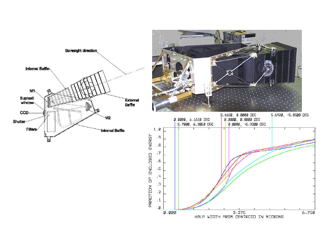
Another way of characterizing the PSF is by giving the
encircled energy
as a function of radius, or at some specified
radius.
A final way of characterizing the image quality, more commonly
used in adaptive optics applications, is the
Strehl ratio SR
. The
Strehl ratio is the ratio between the peak amplitude of the PSF
and the peak amplitude expected in the presence of diffraction
only. In practice, in the visible it is already very good reaching
SR
=
0.1
.
23/02/05
C.Barbieri Elementi_AA_2004
_05 Sesta settimana
40
The EE of the Rosetta
WAC
The WAC is in space,
so there is no seeing
to worry about, only
the vibrations of the
spacecraft or thermal
distortions of the jitter
of the attitude.
23/02/05
C.Barbieri Elementi_AA_2004
_05 Sesta settimana
41
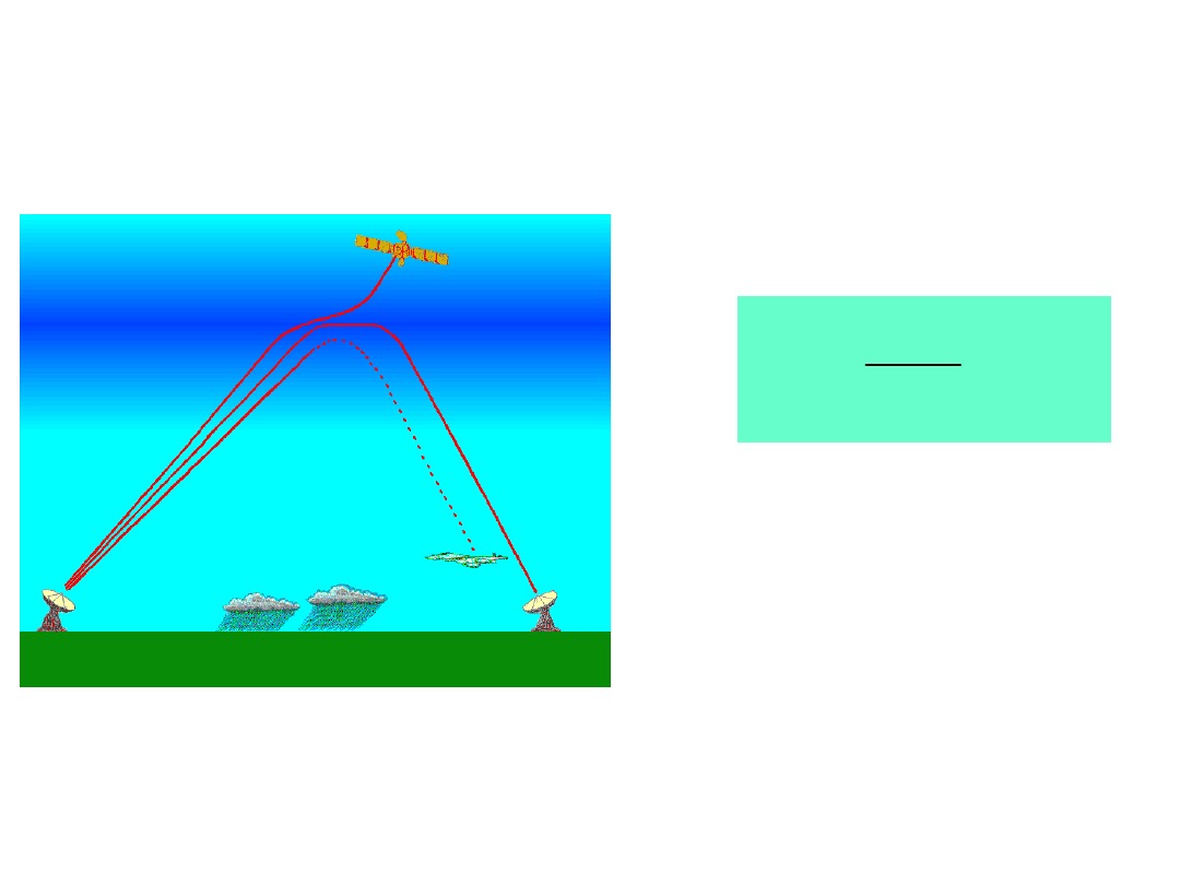
Effects of the atmosphere at
radiofrequencies - 1
The
ionosphere
will
introduce a delay on the
arrival time of the wave,
given by:
2
40.3
d
e
I
T
N s
cn
D =
�
seconds, being
I
the path
along the line of sight and
N
e
the electron density
(cm
-3
). This density will
vary with the night and
day cycle, with the season
and also with the solar
cycle.
23/02/05
C.Barbieri Elementi_AA_2004
_05 Sesta settimana
42
Effects of the atmosphere at
radiofrequencies -2
The tropospheric delay can be resolved in two components, a
dry one and a wet one. The dry component amounts to about 7
ns at the Zenith, and varies with the ‘modified
cosec z
’ we
have discussed for the optical observations:
0.0014
7(cos
) ns
0.0445 cot
t
z
z
D �
+
+
The wet component depends on the amount of water
vapour, and amounts to about 10% of the dry one, but it
varies rapidly and in unpredictable way.
Finally, two other mediums affect the propagation
of the radio waves, namely the
solar corona
and the
ionized interstellar medium
.

23/02/05
C.Barbieri Elementi_AA_2004
_05 Sesta settimana
43
Extinction and
spontaneous emission by
the atmosphere
In addition to chaotic refraction effects, the atmosphere
absorbs
a fraction of the incident light, both in the
continuum and inside atomic and molecular lines and
bands.
Furthermore, the atmosphere spontaneously
emits
in
particular atomic and molecular bands (
this is in addition
to scattering of artificial lights
, see later).
The molecular oxygen
O
2
in particular is so effective at
blocking radiation around 6800A and 7600A that
Fraunhofer could detect by eye two dark absorption bands
in the far red of the solar spectrum, bands he called
respectively B and A (he examined the spectra from red to
blue, the current astronomical practice is from blue to
red).

23/02/05
C.Barbieri Elementi_AA_2004
_05 Sesta settimana
44
Extinction
Let us consider the absorption due to a thin layer of
atmosphere at height between
h
and
h+dh
in the usual
simple model of a plane-parallel atmosphere. The light beam
from the star makes an angle
z
with the Zenith, so that the
traversed path is
dh/cosz = seczdh
.
If
I
(h)
is the intensity at the top of the layer, at the exit it
will be reduced by the quantity:
d
( ) ( )sec d
I
I h k h
z h
l
l
l
=-
In total, if
I
()
is the intensity outside the atmosphere, at
the elevation
h
0
of the Observatory the intensity will be
reduced to:
0
0
sec
( ) d
( ) sec
( )
( )
( )
h
z k h h
z
I h
I
e
I
e
l
l
l
l
l
t
�
-
�
-
��
=
�
=
�
�

23/02/05
C.Barbieri Elementi_AA_2004
_05 Sesta settimana
45
Optical Depth
where we have introduced the a-dimensional quantity
called
optical depth
:
d
( ) d
k h
h
l
l
t =
�
0
( ) d
h
k h
h
l
l
t
�
=
�
�
The variable
k
(dimensionally, cm
-1
) represents the
absorption per unit length of the atmosphere at that
wavelength.
Astronomers use a particular measure of the apparent
intensity, namely the magnitude, defined by
m
=
m
0
-2.5log
I
(see in a later lecture), so that:
ground
d
2.5 ( ) sec
outsi e
m
m
D
z
l
=
-
� �
D
is called the optical density of the atmosphere, while the
variable
X(z)
=
secz
is called
air-mass
. The minimum value of
the airmass is 1 at the Zenith, and 2 at
z
= 60° (the limit of
validity of the present approximate discussion).

23/02/05
C.Barbieri Elementi_AA_2004
_05 Sesta settimana
46
The Bouguer line
Suppose we start observing the star at its upper transit, and
then keep observing it while its Hour Angle (and therefore also
its Zenith distance) increases: we would notice a linear increase
of its magnitude in agreement with the previous equation,
namely
a straight line
with slope
2.5D
in a graph (
m
, sec
z
).
It is common practice to plot the
m
-axis pointing down. This
straight line is known as
Bouguer line
, from the name of the
XVIII century French astronomer who introduced it.
The extrapolation of this line to
X
= 0 (a mathematical
absurdity) gives the so-called
loss of magnitude at the Zenith
, or
else the magnitude outside atmosphere.
According to the formulae of the first lectures we have:
1
sec
( )
sin sin
cos cos cos
z
X z
HA
j
d
j
d
=
=
+
where
is the latitude of the site,
and
HA
the coordinates
of the star.

23/02/05
C.Barbieri Elementi_AA_2004
_05 Sesta settimana
47
The least continuous
extinction
The Table shows the continuous extinction of the
atmosphere above Mauna Kea, whose elevation above sea
level (4300 m) is higher than that of most observatories so
that the transparency of the sky is at its best, in the
extended visible region.
Wavelength (nm)
Extinction
(mag / air mass)
Wavelength
(nm)
Extinction
(mag / air mass)
310
1.37
500
0.13
320
0.82
550
0.12
340
0.51
600
0.11
360
0.37
650
0.11
380
0.30
700
0.10
400
0.25
800
0.07
450
0.17
900
0.05
23/02/05
C.Barbieri Elementi_AA_2004
_05 Sesta settimana
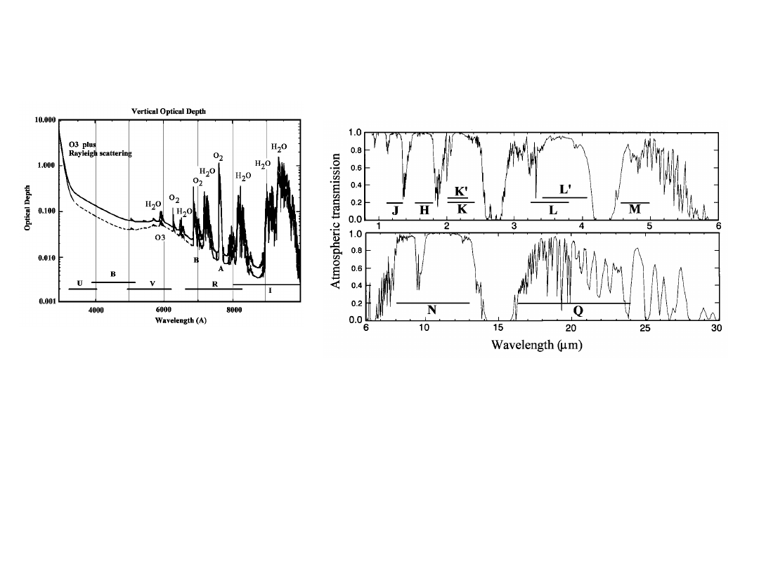
48
Figures of the extinction from the
visible to the near IR
The figure on the left gives the optical depth, the one on the
right the transmission (one is the reverse of the other). In the
violet region, the transparency quickly goes to zero, essentially
because of the ozone
O
3
molecular absorption; at the other end
of the spectrum the transparency is reasonably good until about
2.4 micrometers, when the
H
2
O
and
CO
2
molecules heavily
absorb the light.
The astronomical photometric wide bands (U,B,V, R, I, J, H, …)
are indicated.

23/02/05
C.Barbieri Elementi_AA_2004
_05 Sesta settimana
49
Spontaneous and artificial
emissions
To complete these considerations about the influence of the
atmosphere on the photometry (and also on the spectroscopy)
of the celestial bodies, we must add that the atmosphere
contributes radiation, by spontaneous emission and by
scattering of natural and artificial lights. If the Observatory is
close to populated areas,
bright emission lines of Mercury and
Sodium
from street lamps are observed: Hg at
4046.6,
4358.3, 5461.0, 5769.5, 5790.7; Na at 5683.5, 5890/96 (the
yellow D-doublet), 6154.6; Ne at 6506, and so on.
Natural lines
come from the atomic Oxygen in forbidden
transitions (designated with [OI]) at
5577.4, 6300 and 6367,
and especially from the molecular radical
OH
who provides a
wealth of spectral lines and bands filling the near-IR region
above 6800A.
The OH comes from the dissociation of the water
vapor molecule under the action of the solar UV radiation
.
Therefore, the atmosphere is a diffuse source of radiation,
whose intensity strongly depends on the Observatory site; to
set an indicative value in the visual band, a luminosity
equivalent to one star of 20
th
mag per square arcsec at the
Zenith can be assumed.
23/02/05
C.Barbieri Elementi_AA_2004
_05 Sesta settimana
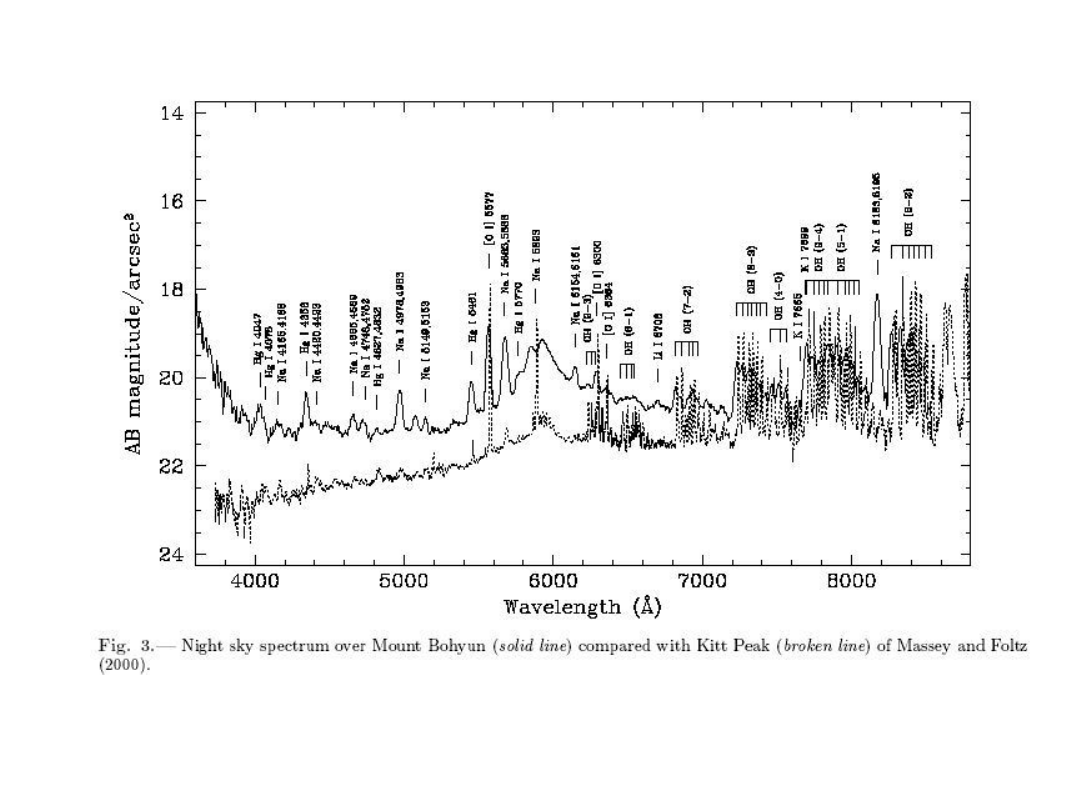
50
The visible spectrum of the
night sky
The night sky is calibrated (see ordinate) in surface brightness, given
as mag/(arcsec)
2
. Mt. Boyun is in Korea.
23/02/05
C.Barbieri Elementi_AA_2004
_05 Sesta settimana
51
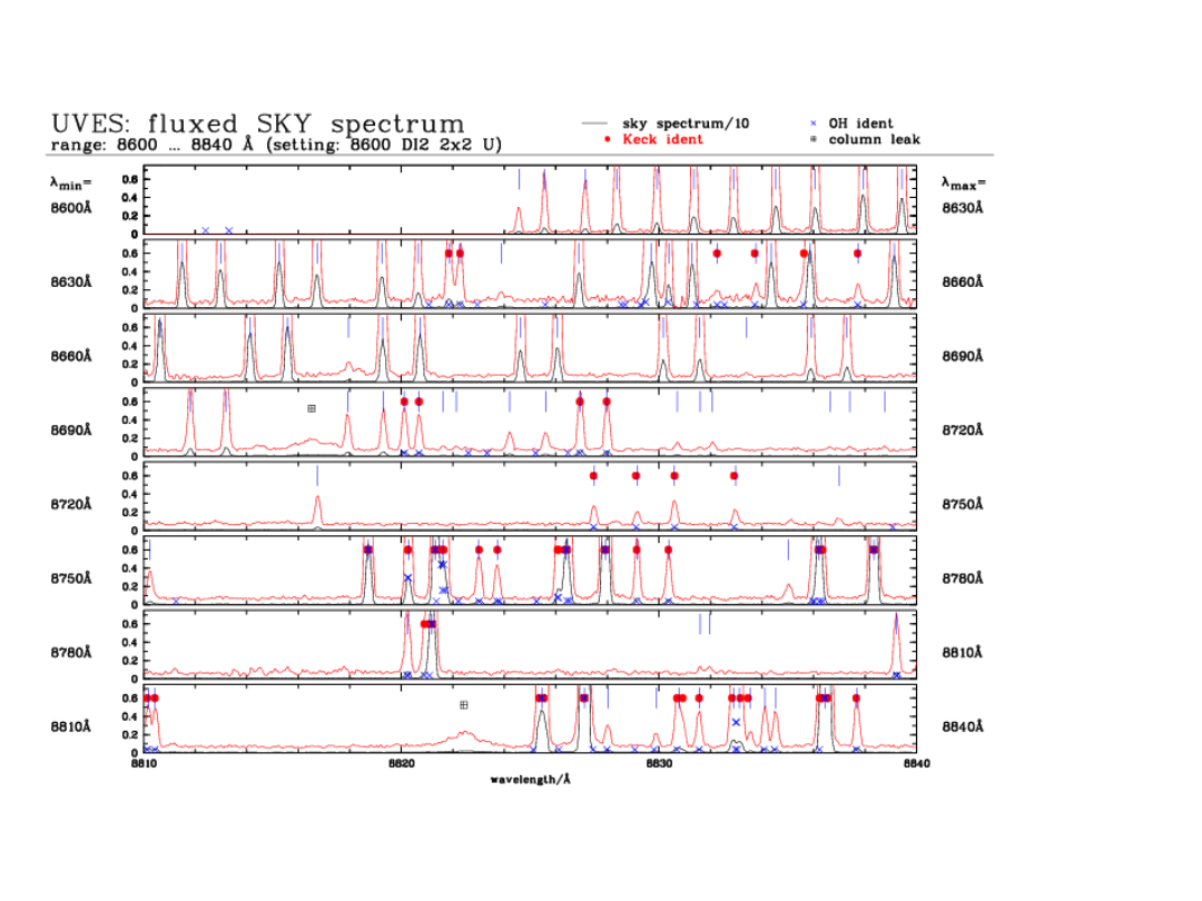
The Near-IR sky emission
- 2
A very
detaile
d
section
of the
near-IR
night
sky
OH-
emissio
n
obtaine
d at
ESO
Paranal
with
UVES.
http://www.eso.org/observing/dfo/quality/UVES/uvessky/sky_8600U_1.html
23/02/2005
C.Barbieri Elementi_AA_2004
_05 Sesta settimana
52
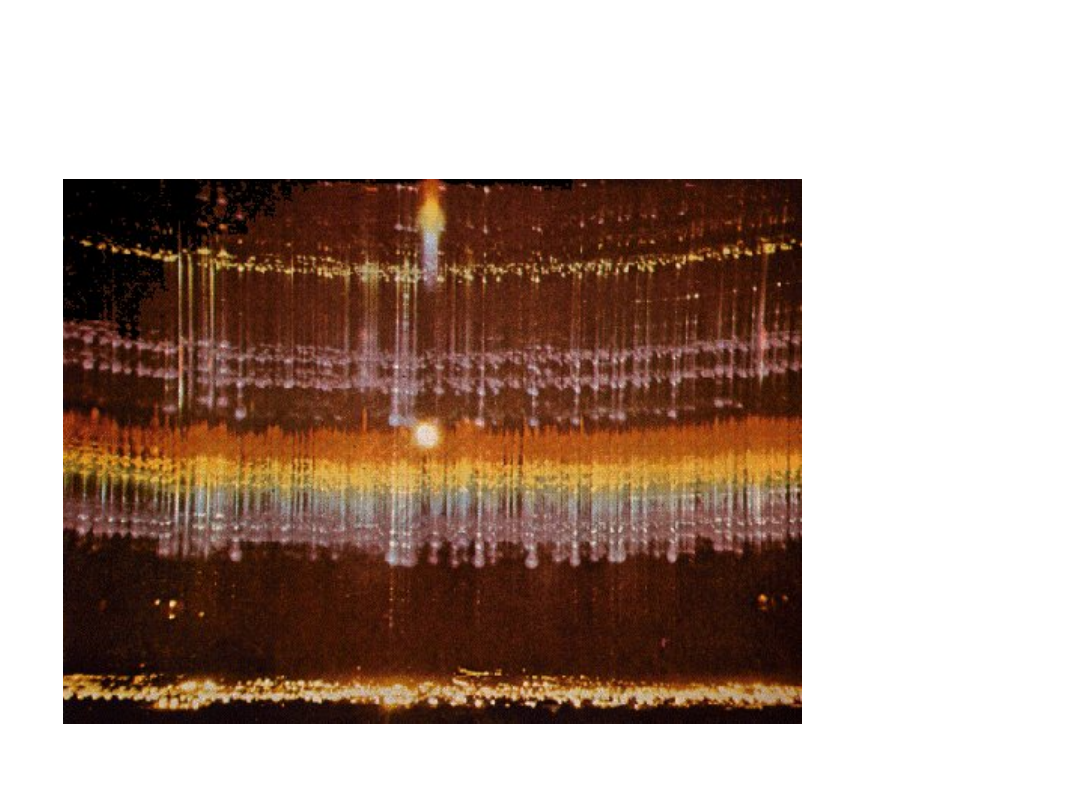
A second limit of the terrestrial
atmosphere: the artificial lights
The full
Moon has
difficulties
in
competing
with the
spectrum
of artificial
lights
.
23/02/2005
C.Barbieri Elementi_AA_2004
_05 Sesta settimana
53
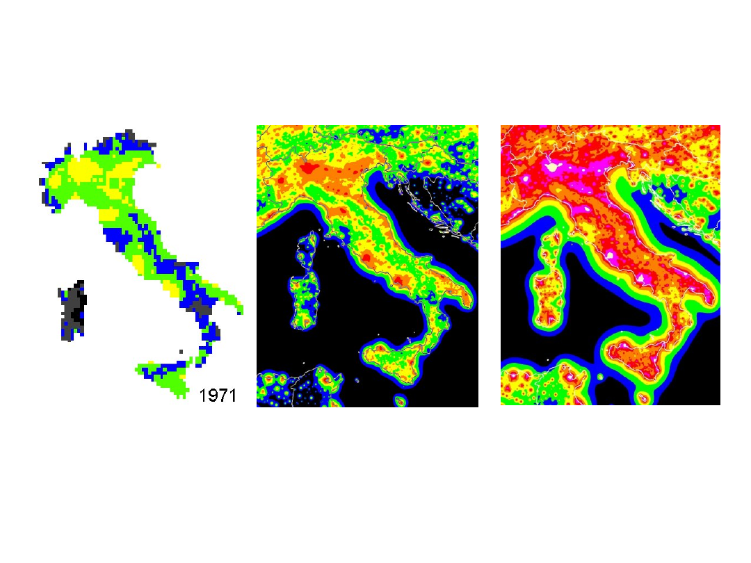
The situation in Italy
1998
2025
If the extrapolation is correct, in 2025 no Italian
will be able to see the Milky Way
23/02/2005
C.Barbieri Elementi_AA_2004
_05 Sesta settimana
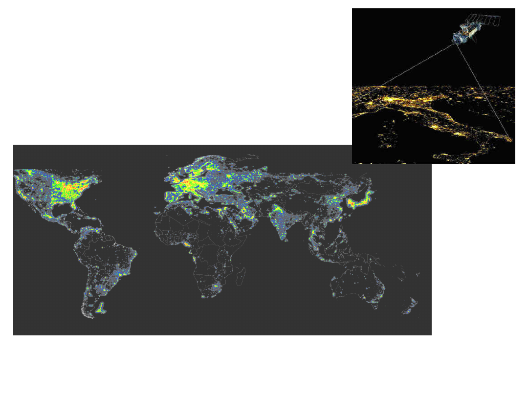
54
Planetary light
pollution
From a paper by Cinzano, Falchi e Elvidge (2001)
23/02/05
C.Barbieri Elementi_AA_2004
_05 Sesta settimana
55
A first exercise of celestial
mechanics
Consider the total energy
E
of a particle
P
2
of very small mass
m
2
at the surface of a non-rotating spherical body
P
1
of radius
R
and mass
m
1
:
2
1 2
2
1
2
mm
E
mV
G
r
=
-
The limiting velocity
V
e
:
1
e
2Gm
V
R
=
is said escape velocity from body
P
1
. If by some means we
impart to
P
2
a velocity V greater than
V
e
in any direction
,
P
2
will reach infinity with final velocity greater than zero.
Another useful critical velocity is that on the
circular orbit
at
distance
r>R
from the center of
P
1
; from the equilibrium
between centrifugal and gravitational forces we get:
2
2
1 2
2
2
c
mV
mm
G
r
r
=
1
c
( )
Gm
V r
r
=
c
e
1
( )
2
V R
V
=
23/02/05
C.Barbieri Elementi_AA_2004
_05 Sesta settimana
56
Escape velocities from the 9
planets
The table provides escape and circular velocities for the 9 planets,
neglecting their diurnal rotation. The 3
rd
column gives the surface
gravity in comparison with that at the Earth’s surface (9.78 m/s
2
). The
first two velocities (4
th
and 5
th
column) pertain to the equator of each
body; the other two velocities (6
th
and 7
th
column) to the circular orbit at
the average distance of the body from the Sun.
Body
Distanc
e
(AU)
Mass
(g)
Radius
(km)
g/g
V
e
(km/s)
V
c
(km/s)
V
e
(⊙)
(km/s
)
V
c
(⊙)
(km/s
)
Sun
1.9910
33
6.9610
5
27.9
618
437
Mercur
y
0.387
3.310
26
2439
0.3
4.3
2.5
96
68
Venus
0.723
4.910
27
6051
0.9
10.4
7.3
49
35
Earth
1.000
6.010
27
6378
1.0
11.2
7.9
42
30
Moon
1.000
7.310
25
1738
0.2
2.4
1.6
42
30
Mars
1.524
6.410
26
3393
0.4
5.0
3.6
34
24
Jupiter
5.203
1.910
30
71492
2.3
59.6
42.5
18
13
Saturn
9.539
5.710
29
60268
0.9
35.5
25.0
14
10
Uranus
19.191
8.710
28
25559
0.8
21.1
15.5
10
7
Neptun
e
30.061
1.010
29
24764
1.1
23.6
16.0
7
5
Pluto
39.529
1.310
2
5
1150
0.04
1.1
0.8
7
5
23/02/05
C.Barbieri Elementi_AA_2004
_05 Sesta settimana
57
Escape velocities and
atmospheres - 1
These considerations on escape velocities from the planetary
surfaces are useful not only for dynamical questions,
but also
for the understanding of their atmospheres
. Let
T
(in
Kelvin) be the temperature of such an atmosphere, supposed in
thermal equilibrium; the distribution function of molecules of
mass
m
2
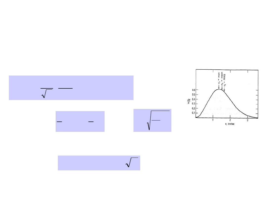
among the velocities is given by Maxwell’s law:
dN V
N m
kT
V e
dV
mV
kT
( )
/
/
F
H
G IKJ
4
2
2
3 2
2
2
2
2
so that the mean square velocity of those
molecules will be:
1
2
3
2
2
2
mV
kT
V
m
kT
3
2
where
k
= 1.3810
-16
erg/K is Boltzmann constant. For
instance, the mass of the Hydrogen atom H is
m
2
1.610
-24
g, so that:
V T
T
H
( )
.
16 10
1
km/s (
T
in K)
At the surface of the Earth, assuming
T
290 K we get
V
H
2.7
km/s <<
V
e
.

23/02/05
C.Barbieri Elementi_AA_2004
_05 Sesta settimana
58
Escape velocities and
atmospheres - 2
All other molecules being heavier than the atom of H, we conclude
that the Earth
is well capable of retaining a substantial quasi-
stationary atmosphere
. However, Maxwell’s distribution has a
very long tail at high velocity, so that a fraction of the Earth’s
gases, and in particular of H, will continuously escape to the outer
space. The observational evidence of such loss is the so-call
geocorona
, well visible in the Ly- spectral line at
= 1216A.
Mercury and the Moon do not have such capability; their tenuous
atmospheres must be continuously lost by thermal escape and
replenished by phenomena such as UV solar photons and solar
particles impinging on the soil and extracting gases, or by
meteoroid bombardment.
In the case of the Sun, the surface gravity is 28 times that at the
surface of the Earth, and the photospheric temperature is
approximately 5800 K; higher up, in the cromosphere and in the
corona, the temperatures of the solar gases rise to tens, hundreds
and even millions of degrees, so that the thermal escape becomes
conspicuous. However, observations prove that the loss of
particles from the Sun (the so-called
solar wind)
is orders of
magnitude larger than that accounted for by thermal loss: other
more efficient mechanisms, whether magnetic or electric, must
act to accelerate the ionized (electrically charged) particles
escaping from the Sun.
23/02/05
C.Barbieri Elementi_AA_2004
_05 Sesta settimana
59
A second exercise of celestial
mechanics
Let us launch from the surface of a spherical non-rotating
Earth of radius
a
⊕
a satellite of mass
m
2
with initial velocity
V
> V
e
. Its energy will be:
2
2
2
1
2
mM
E
mV
G
a
�
�
=
-
(
m
2
<<
M
⊕
)
At an altitude
H
, the distance from the centre becomes
r = a
⊕
+ H
, and the energy:
2
2
2
1
2
r
mM
E
mV
G
r
�
=
-
or else, equating the two values for the conservation of the
energy:
2
2
2
2
2
2
1
1
2
2
r
mM
mM
E
mV
G
mV
G
a
r
�
�
�
=
-
=
-
2
2
1 1
2
r
V
V
GM
a
r
�
�
�
�
=
-
-
�
�
�
�

23/02/05
C.Barbieri Elementi_AA_2004
_05 Sesta settimana
60
Delta V
At infinity:
2
2
2
e
e
e
e
(
)(
) 2
V
V
V
V V V V
V V
�
=
-
= -
+
� D
In conclusion, if we launch with V = + 1km/s, the satellite will
reach infinity with a velocity of approximately 4.7 km/s
(
ignoring the very small losses of energy due to the
atmospheric drag
). There are several practical consequences
of this ‘gain at infinity’, for instance one has to be careful not to
reach the final destination with too high a velocity.
We underline the convenience of using in space
applications the parameter V instead of the energy
.
The circular velocity at the surface of the Earth is
around 8 km/s, which will also be the velocity of low altitude
satellites (e.g. the International Space Station at 300 km).
Their period is then of approximately 90 minutes; suppose we
place such satellite in a polar orbit: it will go out of phase with
the Sun by about 30 min at each orbit, and for several orbits it
will see an almost constant illumination (day or night) of its
Nadir. The low polar orbit is therefore used for surveillance.

23/02/05
C.Barbieri Elementi_AA_2004
_05 Sesta settimana
61
Geostationary orbits
At
H
= 36.000 km the orbital period becomes of 24h, so
that a satellite placed on the equatorial plane at this
altitude in a circular orbit (e.g. the Meteosat) will be
practically stationary with respect to the ground observer.
Actually, several satellites have simply a
geosynchronous
orbit (that was the case of the International Ultraviolet
Explorer), slightly different from the rigorously defined
geostationary one.
At any rate, the two body condition is a
mathematical
abstraction
, several perturbing forces (like the Earth-
Moon and solar tides, the non-sphericity of the Earth
potential, the radiation pressure, etc.) will act to perturb
the orbit, and
appropriate corrections
must be performed
to keep the wanted position of the satellite, for instance by
occasional firings of small thrusters.
Document Outline
- Slide 1
- Slide 2
- Slide 3
- Slide 4
- Slide 5
- Slide 6
- Slide 7
- Slide 8
- Slide 9
- Slide 10
- Slide 11
- Slide 12
- Slide 13
- Slide 14
- Slide 15
- Slide 16
- Slide 17
- Slide 18
- Slide 19
- Slide 20
- Slide 21
- Slide 22
- Slide 23
- Slide 24
- Slide 25
- Slide 26
- Slide 27
- Slide 28
- Slide 29
- Slide 30
- Slide 31
- Slide 32
- Slide 33
- Slide 34
- Slide 35
- Slide 36
- Slide 37
- Slide 38
- Slide 39
- Slide 40
- Slide 41
- Slide 42
- Slide 43
- Slide 44
- Slide 45
- Slide 46
- Slide 47
- Slide 48
- Slide 49
- Slide 50
- Slide 51
- Slide 52
- Slide 53
- Slide 54
- Slide 55
- Slide 56
- Slide 57
- Slide 58
- Slide 59
- Slide 60
- Slide 61
Wyszukiwarka
Podobne podstrony:
podrecznik 2 18 03 05
regul praw stan wyjątk 05
05 Badanie diagnostyczneid 5649 ppt
Podstawy zarządzania wykład rozdział 05
05 Odwzorowanie podstawowych obiektów rysunkowych
05 Instrukcje warunkoweid 5533 ppt
05 K5Z7
05 GEOLOGIA jezior iatr morza
05 IG 4id 5703 ppt
05 xml domid 5979 ppt
Świecie 14 05 2005
Wykł 05 Ruch drgający
TD 05
6 Zagrozenia biosfery 07 05 05
więcej podobnych podstron