Simulation of fatigue failure in a full composite wind turbine blade

Mahmood M. Shokrieh

*

, Roham Rafiee

Composites Research Laboratory, Mechanical Engineering Department, Iran University of Science and Technology, Narmak, Tehran 16844, Iran

Available online 13 June 2005

Abstract

Lifetime prediction of a horizontal axis wind turbine composite blade is considered. Load cases are identified, calculated and

evaluated. Static analysis is performed with a full 3-D finite element method and the critical zone where fatigue failure begins is
extracted. Accumulated fatigue damage modeling is employed as a damage estimation rule based on generalized material property
degradation. Since wind flow (loading) is random, a stochastic approach is employed to develop a computer code in order to sim-
ulate wind flow with randomness in its nature on the blade and subsequently each load case is weighted by its rate of occurrence
using a Weibull wind speed distribution.
Ó 2005 Elsevier Ltd. All rights reserved.

Keywords: Composites; Finite element; Stochastic; Wind turbine blade; Damage; Failure analysis

1. Introduction

Pollution free electricity generation, fast installation

and commissioning capability, low operation and main-
tenance cost and taking advantage of using free and
renewable energies are all advantages of using wind tur-
bines as an electricity generators. Along with these
advantages, the main disadvantage of this industry is
the temporary nature of wind flow. Therefore, using reli-
able and efficient equipment is necessary in order to get
as much as energy from wind during the limited period
of time that it flows strongly.

The blade is the most important component in a wind

turbine which nowadays is designed according to a re-
fined aerodynamic science in order to capture the maxi-
mum energy from the wind flow. Blades of horizontal
axis are now completely made of composite materials.
Composite materials satisfy complex design constraints
such as lower weight and proper stiffness, while provid-
ing good resistance to the static and fatigue loading.

Generally, wind turbines are fatigue critical machines

and the design of many of their components (especially
blades) are dictated by fatigue considerations. Several
factors expose wind turbine blades to the fatigue phe-
nomena which can be summarized as shown below

[1]

:

1. Long and flexible structures
2. Vibrations in its resonant mode
3. Randomness in the load spectra due to the nature of

the wind

4. Continuous operation under different conditions
5. Low maintenance during lifetime

A wind turbine blade expects to sustain its mission

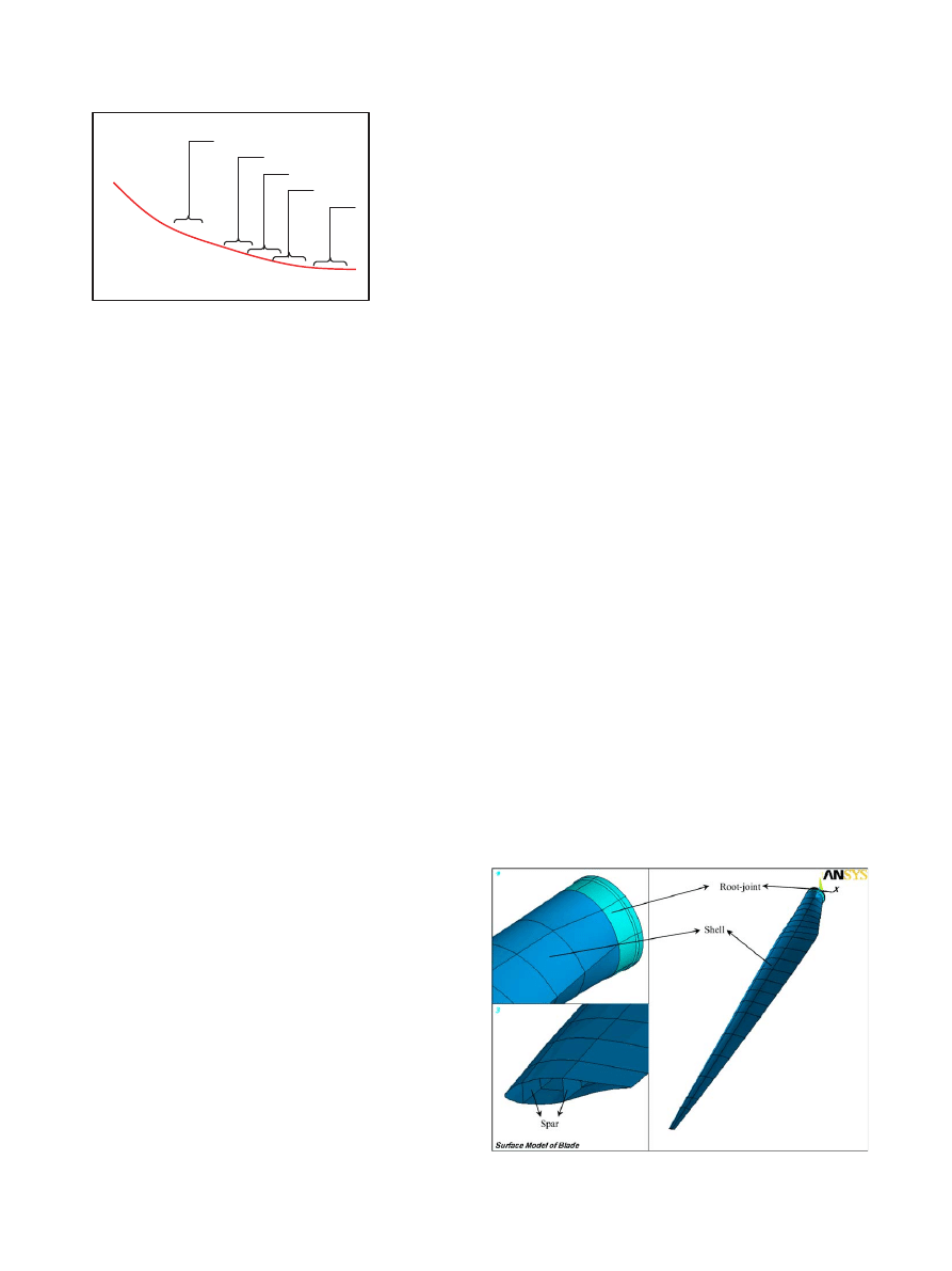
for about 20–30 years.

Fig. 1

shows a comparison be-

tween different industrial components and their expected
life cycles.

The above mentioned reasons and extensive expected

lifetime cause design constraints for wind turbine struc-
tures that fall into either extreme load or fatigue catego-
ries. For the case of extreme load design, the load
estimation problem is limited to finding a single maxi-
mum load level that the structure can tolerate. For de-
sign against fatigue, however, loads must be defined

0263-8223/$ - see front matter

Ó 2005 Elsevier Ltd. All rights reserved.

doi:10.1016/j.compstruct.2005.04.027

*

Corresponding author. Tel./fax: [phone].
E-mail address:

[e-mail]

(M.M. Shokrieh).

Composite Structures 74 (2006) 332–342

www.elsevier.com/locate/compstruct

for all input conditions and then summed over the distri-
bution of input conditions weighted by the relative fre-
quency of occurrence.

Most ongoing research on fatigue phenomena uses

load spectra obtained by digital sampling of a specific
configuration of strain gauges which read the strain at
a specific location near the root of blade. Then, the rep-
resentative sample of each load spectrum is weighted by
its rate of occurrence that can be obtained from the sta-
tistical study of the wind pattern. Finally all weighted
load spectra are summed and total load spectrum is de-
rived. This load spectrum is utilized to estimate fatigue
damage in the blade using MinerÕs rule

[2]

. One of the

main shortcomings of this method is the linear nature
of MinerÕs rule. Not only is MinerÕs rule not a proper
rule for fatigue consideration in metals, but also it has
been proven that this rule is not suitable for composites

[3]

. Another problem with using MinerÕs rule is the

weakness of this model to simulate the load sequence
and history of load events. This shortcoming can clearly
be seen in the difference of predicted lifetimes of blades
with two orders of magnitudes for two load cases with
different load sequences

[2]

. Furthermore, most investi-

gations in fatigue simulation of composite blades are
limited to the deterministic approach. In addition, iden-
tification of a place to install the strain gauges in order
to extract the load spectrum is also questionable. Using
a massive and high cost material fatigue database

[4]

, is

another problem with these methods. It forces research-
ers to characterize each configuration of lay-up sepa-
rately and is the main reason for publishing new
versions of these databases each year due to introduc-
tion of new lay-up configurations in blade structure by
industry.

2. State of the art

In this paper, a model to study the fatigue phenom-

ena for wind turbine composite blades is presented in
order to overcome the aforementioned shortcomings

of current methods. As a case study, a 23 m blade of a
V47-660 wind turbine, manufactured by the Vestas
Company, was selected. Firstly, loading on the blade
is considered carefully using the finite element method
and the critical zone where catastrophic fatigue failure
initiates is determined. Then, each load case is weighted
and finally fatigue is studied using a developed stiffness
degradation method. The main advantages of this meth-
od can be expressed in its ability to simulate the load se-
quence and load history. Due to randomness of wind
flow; stochastic analysis will be employed instead of
deterministic analysis. Based on the capability of the
method for fatigue modeling, performing a large quan-
tity of experiments in order to characterize complete fa-
tigue behavior of materials is avoided.

3. Modeling

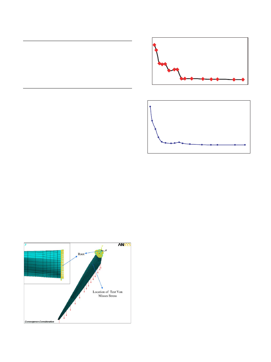
The investigated blade consists of three main parts

called shell, spar and root-joint (see

Fig. 2

).

The shell is responsible to help create the required

pressure distribution on the blade. The cross sections
of the blade are different airfoils based on aerodynamic
considerations. The shell also twists about 15

° due to

aerodynamic reasons and also has a tapered shape from
root to tip.

A brief summary of pertinent data related to the

investigated blade is shown in

Table 1

.

The spar, which is also called the main beam, has to

support loads on the blade that arise from different
sources. The shell structure carries only 20% of total
loads while the rest has to be carried by the spar. The
cross section of the spar has a box shape.

The root joint is the only metallic part in the current

blade that connects whole blade structure to the hub by
screws. This metallic joint is covered by composite lam-
inates internally and externally.

Fig. 2. Depiction of root-joint, shell and spar.

Number of Fatigue Cycles to Failure

Allowable Cyclic Stress

Commercial Aircraft

Bridges

Hydrofoils

Helicopter

Wind Turbine Blade
20-30 year Life

10

5

10

6

10

7

10

8

10

9

Fig. 1. Schematic S–N curves for different industrial components

[1]

.

M.M. Shokrieh, R. Rafiee / Composite Structures 74 (2006) 332–342

333

In order to provide data for the finite element model,

a geometrical model was created based on cross section
profiles of shell and spar using Auto-CAD

[5]

software.

Then the wire frame model, which is the fundamental
geometrical model, was transferred to ANSYS finite ele-
ment software

[6]

. After that, geometrical modeling was

completed by creating surfaces using the loft method. In
the meshing process, second order shell elements were
employed to increase accuracy of the modeling. In addi-
tion, the selected element type is compatible with com-
posites and, in order to not having any triangular
elements, a manual meshing method was employed.
Therefore all elements have quadratic shape with 8
nodes and acceptable aspect ratio. Elements of the
root-joint segment are second order cubic solid
elements.

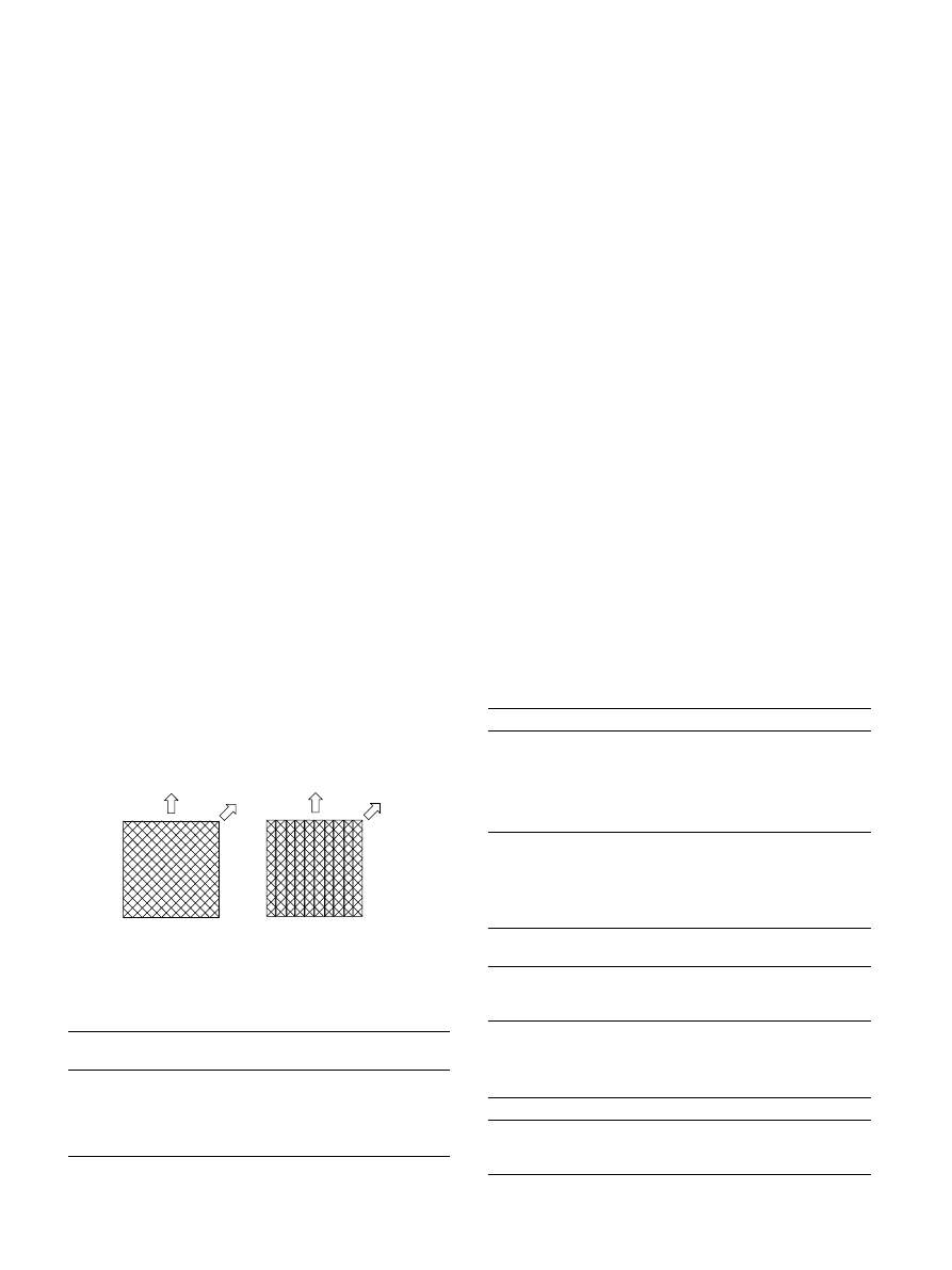
Convergence criteria should be considered to evalu-

ate the results. Convergence analysis is performed on a
metallic model of the blade. By improving mesh density
step-by-step a suitable number of elements is obtained.
The stabilization of tip deflection and Von-Misses equiv-
alent stress at a location far from the applied loads
are the criteria of convergence. Also in order to examine
the case with both bending and torsion in the structure,
the loads were applied on the trailing edge and bound-

ary conditions consisted of fixing all 6 degrees of free-
dom of nodes that are placed at the root. The
depiction of the FE model is shown in

Fig. 3

.

Fig. 4

shows the results of convergence analysis.

From

Fig. 4

, it is clear that convergence is obtained with

the use of about 10,000 or more elements.

4. Material characterization

The investigated blade consists of three main types of

pre-preg glass/epoxy composites: Unidirectional plies,
bi-axial and tri-axial materials.

Bi-axial and tri-axial plies contain two and three

same unidirectional fabrics, respectively, which are
stitched together (thus are not woven). The main reason
for not using woven form of composites is due to disad-
vantages of using them based on their fatigue properties.
In the woven form, due to out-of-plane curvature of
fabrics, stress concentrations happen and consequently
fatigue performance of these materials decreases dra-
matically

[3]

.

Tri-axial and bi-axial fabrics are used in the shell

structure and unidirectional and bi-axial are used in
the spar structure. The configuration of the bi-axial lam-
ina is [0/90]

T

and the configuration of the tri-axial lam-

inate is [0/+45/

45]

T

. Two kinds of foam (PMI and

PVC) are used respectively at the spar and shell loca-
tions, respectively, in order to construct the sandwich
panel.

Table 1
General specifications of investigated blade

Length

22,900 mm

Maximum chord

2087 mm

Station of maximum chord

R4500

Minimum chord

282.5 mm

Twist

15.17

°

Station of CG

R8100

Weight of blade

1250 kg

Tip to tower distance

4.5 m

Surface area

28 m

2

Airfoil cross-section types

FFA-W3, NACA-63-xxx, MIX

Fig. 3. Finite element model of turbine blade showing loads and
boundary conditions for convergence consideration.

Convergency Based on Stress

600

1092

6604

23712

21312

17016

15418

13232

10284

8508

7664

5728

4358

2634

3428

1876

Number of Elements

Von Misses Stress

Convergency Based on Deflection

600

1092

1876

2634

6604

5728

4358

3428

8508

10284

13232

15418

17016

7664

21312 23712

Number of Elements

Tip Deflection

Fig. 4. Convergence graphs of FE model.

334

M.M. Shokrieh, R. Rafiee / Composite Structures 74 (2006) 332–342

The required properties for analyzing the structure

are mechanical and strength properties where the first
group is used for stress analysis and the second one is
used for failure analysis

[7]

. Material characterization

is used to extract the aforementioned properties. Full
material properties of the U-D fabric are available
experimentally

[4]

but for the bi-axial and tri-axial com-

posites, the mechanical properties are not complete. The
available data of these materials are limited to the elastic
modulus in the 0

° and 45° directions

[8]

. The bi-axial

and tri-axial laminates and the direction where the
experimental results are available are shown in

Fig. 5

.

The available experimental data are summarized in

Table 2

.

As it can be seen from

Table 2

, elastic modulus E

1

and E

2

are equal in both [+45/

45]

T

and [0/90]

T

and

[0/90/

45]

T

due to symmetry.

4.1. Extracting non-available mechanical properties

First, stiffness matrices of tri-axial and bi-axial mate-

rials are calculated by considering the proportion of fab-
ric in each direction and then the matrices were inversed.
In parallel, compliance matrices based on available data
were made and finally the recently obtained compliance
matrices were compared to the previously extracted
compliance matrices from the stiffness matrices. Finally,
after omitting redundant equations, the remaining ones
form 14 sets of equations with 14 unknowns enabling
the solution for the mechanical properties of constructed
unidirectional plies.

Those equations are not reported here due to space

limitations and complete list of the governing equations

can be found in Ref.

[9]

. Due to this fact that those 14

equations are highly dependent and nonlinear, solving
them by conventional method is impossible and it needs
a start point. The best suggestion for a starting point is
the PoissonÕs ratio for the bi-axial material in configura-
tion of [0/90]

T

. Experiments show that the PoissonÕs

ratio of [0/90]

T

configuration is somewhere between

0.05 and 0.1 and these values also are verified by theory

[10]

. In

Table 3

, the results obtained by using different

amount of PoissonÕs ratio are summarized.

As can be seen, the best results are achieved when

PoissonÕs ratio is set to 0.06 because of its E

Y

. Therefore,

mechanical properties of unidirectional plies are avail-
able from experiments

[4]

and mechanical properties of

bi-axial and tri-axial laminates can be calculated based
on the technique in this research and using mechanical
properties of their constructed U-D ply which is calcu-
lated and inserted in

Table 3

. The mechanical properties

are summarized in

Table 4

.

If we calculate the flexural modulus using the ob-

tained data, there is very good agreement to the experi-
mentally available value for this parameter as shown in

Table 5

.

One of the main advantages of using the inverse

method can be realized in the fatigue modeling method
that is employed in this paper and will be discussed later
in detail.

45˚

0˚

0˚

45˚

Biax Laminate

Triax Laminate

Fig. 5. Experiment directions of bi-axial and tri-axial laminates.

Table 2
Available and non-available mechanical properties

[4,8]

Composites

Configuration E

1

[GPa]

E

2

[GPa]

m

12

E

6

[GPa]

Unidirectional

–

43

9.77

0.32

3.31

Bi-axial

[±45]

T

6.8

6.8

N/A

a

N/A

Bi-axial

[0/90]

T

16.7

16.7

N/A N/A

Tri-axial

[0/±45]

T

20.7 ± 3.1 N/A

N/A N/A

Tri-axial

[0/90/

45]

T

15.1 ± 2.3 15.1 ± 2.3 N/A N/A

a

N/A: Not available.

Table 3
Mechanical properties of constructed U-D ply varied by change in
major PoissonÕs ratio of bi-axial laminate

MPB

a

E

X

[GPa]

E

Y

[GPa]

m

G [GPa]

0.05

28.549

4.5643

.21

2.107

0.06

28.892

4.3624

.26

2.096

0.07

29.010

4.2215

.32

2.090

0.08

29.127

4.100

.37

2.085

0.09

29.197

3.8240

.40

2.080

0.10

29.234

3.6942

.43

2.077

a

MPB: Major PoissonÕs ratio of bi-axial [0/90]

T

.

Table 4
Mechanical properties of involved materials in the blade

E

1

[GPa]

E

2

[GPa]

Major
PoissonÕs ratio

G

XY

[GPa]

Unidirectional ply

43

9.77

0.32

3.31

Bi-axial [0/90]

T

16.7

16.7

0.06

2.01

Tri-axial [0/+45/

45]

T

17.6

7.01

0.52

5.07

Table 5
Experimental and theoretical comparison of flexural modulus

Tri-axial [0/90/

45]

Tri-axial [0/45/

45]

Flexural

modulus

Experimental

[8]

Theoretical

Experimental

[8]

Theoretical

15.1 ± 2.3

15.23

16.7 ± 2.5

17.85

M.M. Shokrieh, R. Rafiee / Composite Structures 74 (2006) 332–342

335

The last step of this stage is devoted to extracting the

weight of the finite element model and comparing it with
realistic data. These data are shown in

Table 6

and de-

scribe the health of model from lay-up configuration
and prove that the model is in a good accordance with
actual structures.

5. Loading

The load cases are determined by the combination of

specific operating and external conditions. Operating
and external conditions are assumed to be statistically
independent

[11]

. Operating conditions divided into four

groups known as normal, fault, after occurrence of the
fault and transportation, erection and maintenance
(see

Fig. 6

). External conditions are divided into two

groups called normal and extreme. The load cases to
be used for fatigue analysis generally arise only from
the combination of normal external and operating con-
ditions. It is assumed in this context that because they
occur so rarely, the other combinations will not have
any significant effect on fatigue strength

[11]

.

The involved subgroups of normal operating and

normal external conditions are shown in

Fig. 6

.

All of the load cases that occur during the mentioned

events can be categorized as follows:

1. Aerodynamic loads on the blade
2. Weight of the blade
3. Annual gust
4. Changes in the wind direction
5. Centrifugal force
6. Force that arise from start/stop angular acceleration
7. Gyroscopic forces due to yaw movements
8. Activation of mechanical brake
9. Thermal effect

All of the above load cases were calculated and it was

evident that gyroscopic forces and forces from mechan-
ical brake activation can be ignored in comparison with
the other loads

[12]

. A temperature range was consid-

ered between

10° and +40° according to the surround-

ing ambient environment.

6. Static analysis

At the first step of static analysis, in order to insure

that the model is compatible with real structures, a free
vibration analysis of model is performed

[12]

. The result-

ing data are in a good agreement with experimental data

[12]

. The results of free vibration analysis show that

model is in accordance with real structures from differ-
ent aspects such as dimension, material properties and
lay-up sequence.

In the second step, calculated forces from the previ-

ous section are applied and the response of the structure
is studied. In some cases, performing non-linear analysis
was necessary due to large rotation effects as a source of
non-linearity. The results of these analyses are summa-
rized in

Table 7

.

Table 6
Mass comparison of the blade

Mass [kg]

CG location [mm]

FE model

1268.45

7575.23 (from the root)

Realistic

1250.00

7500.00 (from the root)

Stand-by

Start-up

Power

Production

Normal

Shut-down

Condition

Operating

Conditions

External

Conditions

Normal

Operating

Fault

After the

Occurrence
of the Fault

Transport,

Erection &

Maintenance

Extreme

Normal

Normal Operating

Gust

Temperature Ranges

Changes in the Wind

Direction

Fig. 6. General view of operating and external conditions of a wind turbine.

336

M.M. Shokrieh, R. Rafiee / Composite Structures 74 (2006) 332–342

The safety factor results show that in all cases the

structure is in a safe condition. Knowing that the tip-
to-tower distance of the blade is 4.5 m, then for the max-
imum tip deflection case, tip of the blade will not hit the
tower.

In the third step, the structure is studied under ther-

mal loads and the analysis shows that the temperature
range does not have a significant effect in comparison
with other load cases, so the temperature load was not
considered further.

In the fourth step, buckling phenomena was consid-

ered linearly and non-linearly and obtained results

[12]

indicate that the structure is in a safe condition.

The Tsai–Wu criterion is used to obtain the critical

zone for failure. Furthermore, because of the existence
of a pitch control system on the investigated blade and
a rotation of the blade along its length by wind speed
variation around 89

°, the obtained critical zone by the

Tsai–Wu criteria varied with the change in wind speed.
The results showed that the critical zone can be divided
into five groups for 4–8, 8–12, 12–16, 16–20 and 20–
25 m/s wind speed ranges. From these ranges, the most
probable wind speed range that has the biggest value
as its accumulate wind speed probability is selected as
the most critical zone. This zone is located on the upper
flange of the spars, which has a layup with 11 layers of
0

° and one [+45/45]

T

bi-axial laminate.

Finally, a comparison between normalized longitudi-

nal (N

X

), transverse (N

Y

) and shear forces (N

XY

) to the

length of selected critical zone, proves that the quantity
of N

Y

and N

XY

versus N

X

is negligible and also, consid-

ering normalized moments (M

X

, M

Y

and M

XY

) will not

change the amount of effective stresses significantly. So
it can be concluded that the uni-axial fatigue mode is
dominant for the critical region.

7. Accumulated fatigue damage modeling

One of the presented techniques to investigate fatigue

in composites is called ‘‘Generalized Material Property
Degradation Technique’’ which was developed by Shok-
rieh and Lessard

[13]

. In this research, Shokrieh–Les-

sardÕs method was simplified in order to simulate the
laminated composite behavior under uni-axial fatigue
loading. This model can estimate damage status at any
stress level and number of cycles from start of loading

to sudden failure of the component and can predict final
fatigue life. In order to fulfill the mentioned require-
ments, an accumulated fatigue damage model is sug-
gested based on CLT

1

[14]

. This model contains three

main parts: stress analysis, damage estimation and
material properties degradation. Due to this fact that
the selected critical zone is placed in a confined
region, edge effects will not occur and therefore CLT
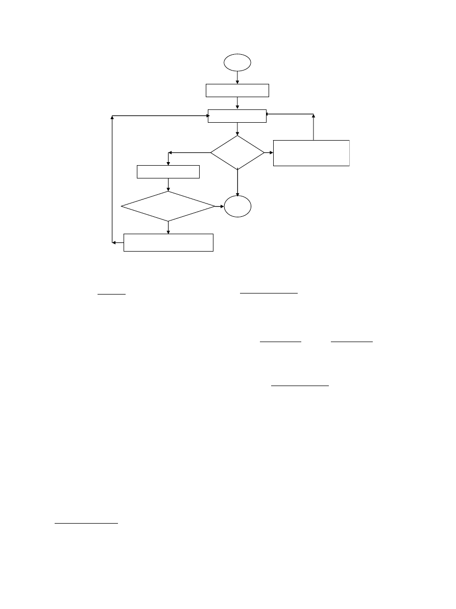
is appropriate. The flowchart of the accumulated fatigue
damage that has been used for developing a computer
code in order to calculate needed parameters is shown
in

Fig. 7

.

As shown in

Fig. 7

, a proper model for stress analysis

must first be developed. In this step, material properties,
maximum and minimum fatigue load, maximum num-
ber of cycles, incremental number of cycles are defined.
Then stress analysis based on CLT theory and loading
condition is preformed. In the next step, failure analysis
is preformed. If there is a sudden mode of failure, then
material properties of the failed plies are changed
according to appropriate sudden material property deg-
radation rules. The stiffness matrix of the finite element
model is rebuilt and the stress and failure analysis are
preformed again. In this step, if there is no sudden mode
of failure, an incremental number of cycles is applied. If
the number of cycles is greater than a preset total num-
ber of cycles, then the computer program stops. Other-
wise, stiffness of all plies (of all elements) is changed
according to gradual material property degradation
rules. Then stress analysis is performed again and the
above loop is repeated until catastrophic failure occurs,
or the maximum number of cycles (pre-defined by the
user) is reached. It is necessary to mention that in the
material property degradation, different methods have
been experienced by several authors for strength degra-
dation or stiffness degradation as a single criteria or
combinations of stiffness and strength degradation as a
combined criterion. In this study, in order to decrease
run-time of model, the stiffness degradation technique
was employed. In this method remaining stiffness of an
U-D ply under desired uni-axial state of stress and de-
sired stress ratio can be calculated using the following
equation which is a modified and improved form of
YeÕs model

[15]

:

Table 7
Static analysis of blade under different events

Events

Tip deflection
[m]

Maximum longitudinal
stress [MPa] (safety factor)

Maximum transverse stress
[MPa] (safety factor)

Maximum in-plane shear
stress [MPa] (safety factor)

Standby

1.23

520.12 (2.22)

13.61 (3.1)

21.33 (3.8)

Start-up

1.67

650.30 (1.79)

12.94 (2.8)

32.50 (2.5)

Power production

4.21

725.00 (1.60)

15.50 (2.3)

18.12 (4.4)

Shut-down

4.33

764.00 (1.52)

19.02 (1.9)

21.27 (3.8)

1

Classical lamination theory.

M.M. Shokrieh, R. Rafiee / Composite Structures 74 (2006) 332–342

337

E

ðn; r; jÞ ¼

1

~

D

f

ðr; r

ult

Þ

E

0

In this equation, E

0

, E(n,r,j) and ~

D

, respectively, rep-

resent initial stiffness before start of fatigue loading,
residual stiffness (as a function of number of cycles, ap-
plied stress and stress ratio) and normalized damage
parameter. Due to the fact that the amount of ~

D

does

not depend on the applied stress level, in order to in-
clude the role of stress in the amount of damage f(r, r

ult

)

is used. A complete form of f(r, r

ult

) was developed

[13]

based on available experimental data for carbon/epoxy
(commercially called AS4/3501-6).

A developed damage estimation method is used to

calculate ~

D

that describes a relation between ~

D

and ~

N

,

which is called the normalized number of cycles. Avail-
able experimental data show that normalized damage
increases linearly from start of loading till ~

N

¼ 0.67

and after that the rate of damage increases non-linearly
until final failure

ð ~

N

¼ 1Þ. So the relation between ~

D

and

~

N

can be divided into two phases. All equations that de-

scribe the linear and non-linear relations between ~

D

and

~

N

are fully constructed for both phases

[16]

. In all afore-

mentioned equations, ~

N

is calculated using following

equation:

~

N

¼

log

ðnÞ logð0.25Þ

log

ðN

f

Þ logð0.25Þ

where, n and N

f

describe number of applied cycles and

cycles to failure respectively. N

f

must be calculated using

following relation

[13]

:

ln

ða=f Þ

ln

½ð1 qÞðC þ qÞ

¼ A þ B log N

f

where

q

¼ r

m

=

r

t

;

a

¼ r

a

=

r

t

;

C

¼ r

c

=

r

t

;

r

m

¼

ðr

max

þ r

min

Þ

2

;

r

a

¼

ðr

max

r

min

Þ

2

It is shown that in shear loading, the aforementioned
equation can be modified to the following form

[13]

:

u

¼ log

ln

ða=f Þ

ln

½ð1 qÞðC þ qÞ

¼ A þ B log N

f

where u and f are curve fitting parameters which have
been obtained for AS4/3501 material

[13]

.

8. Evaluation of accumulated fatigue damage model

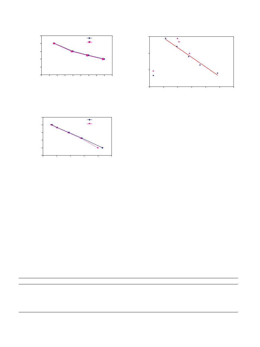
The computer code which has been written on the

Mathematica platform

[17]

, was tested for a 0-degree

U-D ply of carbon/epoxy under tensile longitudinal fati-
gue loading, a 90-degree U-D ply of carbon/epoxy under
tensile transverse fatigue loading and a cross-ply of car-
bon/epoxy. The obtained results in comparison with
available experimental data

[13,18,19]

are shown in

Figs.

8–10

which explain the appropriate performance of

model.

All equations and relations have been developed

based on available experimental data for carbon/epoxy
composites. Since normalized life curves for glass/epoxy

Yes

No

Yes

Start

Model Preparation

Stress Analysis

Failure

Analysis

Cycles = Cycles +

δn

Change Material Properties Based

on Gradual Degradation Rules

Cycles > Total

Cycles

Stop

Change Material Properties

Based on Sudden

Degradation Rules

No

Final

F

ailure

Fig. 7. Flowchart of accumulated fatigue damage modeling.

338

M.M. Shokrieh, R. Rafiee / Composite Structures 74 (2006) 332–342

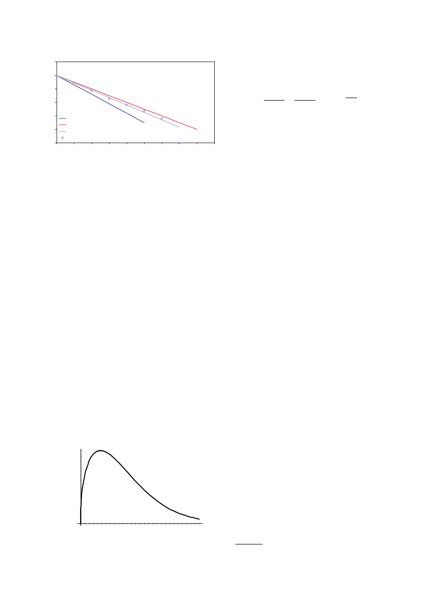
were not available, a generic behavior was estimated
based on the pattern of decreasing mechanical proper-
ties and strengths of carbon/epoxy. The only available
criteria for evaluation of aforementioned generic fatigue
behavior process, is the mentioned criteria in MSU/
DOE fatigue database

[4]

for wind turbine blade appli-

cation. In MSU/DOE, the behavior of involved compos-
ite materials in blade structures is defined by the
following equation

[4]

:

r=r

0

¼ 1 b logðN Þ

where ‘‘r’’ is maximum applied stress and ‘‘r

0

’’ is corre-

sponding static strength in the same direction of applied
stress and finally ‘‘b’’ is a parameter which varies for the

different materials. In MSU/DOE two magnitudes of
‘‘b’’ were presented which describe two boundaries of
all curves. The upper bound refers to good material that
behaves perfectly against fatigue and the lower bound
refers to poor material that behaves weakly. The values
of ‘‘b’’ for different fatigue loading situations are ex-
tracted from the MSU/DOE database

[4]

and inserted

in

Table 8

.

After using the accumulated fatigue damage model,

with aforementioned generic methods, the obtained re-
sults approach the bound of good materials as expected.
For instance, tensile mode results are shown in

Fig. 11

.

Good materials are those with high quality and same
volume of resin at all points containing non-woven fab-
rics

[4]

. Since the pre-preg materials are known as mate-

rials that fulfill the above-mentioned characteristics, it
can be concluded that the obtained results are logical
and generic behavior is appropriate. However, it is nec-
essary to mention that, even though the generic method
is working properly, a more complete treatment would
involve extracting the normalized life curve and other re-
quired parameters specifically for the type of glass/epoxy
used here.

One of the most important advantages of using accu-

mulated fatigue damage modeling is in its independence
of lay-up configuration. Thus it can be used for any con-
figuration of fabrics, knowing behavior of involved U-D

Cross Ply, Tensile Fatigue Loading R = .1

0.6

0.7

0.8

0.9

0

2

4

6

8

10

12

S

=

S

tr

ess/

S

tr

e

n

g

th

Experiment [18,19]

Model

Log (N

f

)

Fig. 10. Experimental data and results of computer code for cross ply.

S=Stress/Strength

0-Degree Ply, Longitudinal Loading

0

0.2

0.4

0.6

0.8

1

0

3

6

9

12

15

18

21

24

27

Experiment [13]

Model

Log (N

f

), Cycles

Fig. 8. Experimental data and results of computer code for 0-degree
ply.

90-Degree Ply, Transverse Loading

0

0.2

0.4

0.6

0.8

1

0

3

6

9

12

15

Experiment [13]

Model

S=St

re

ss/

St

ren

g

th

Log (N

f

), Cycles

Fig. 9. Experimental data and results of computer code for 90-degree
ply.

Table 8
Values of ‘‘b’’ for two bounds of good and poor materials (S–N data)

Type of data

Extremes of normalized S–N fatigue data for fiberglass laminates

Tensile fatigue data (R = r

min

/r

max

= 0.1)

Good materials

Poor materials

Normalization

b = 0.1

b = 0.14

UTS

a

Compressive fatigue data (R = 10)

Good materials

Poor materials

Normalization

b = 0.07

b = 0.11

UCS

b

Reversal fatigue data (R =

1)

Good materials

Poor materials

Normalization

b = 0.12

b = 0.18

UTS

a

Ultimate tensile strength.

b

Ultimate compressive strength.

M.M. Shokrieh, R. Rafiee / Composite Structures 74 (2006) 332–342

339

plies (full characterization of each configuration is not
required).

9. Wind resource characterization

Identification of governing wind patterns on the wind

farm vicinity is necessary for weighting different events
for fatigue analysis. The wind speed is never steady at
any site, but it is rather influenced by the weather sys-
tem, the local land terrain and the height above the
ground surface. Therefore, annual mean speed needs
to be averaged over 10 or more years. Such a long term
average raises the confidence in wind speed distribution.
However, long-term measurements are expensive, and
most projects cannot wait that long. In such situations,
the short term, say one year, data is compared with a
nearby site having available long-term data to predict
the long-term annual wind speed at the site under con-
sideration. This is known as the ‘‘measure, correlate
and predict (MCP)’’ technique. Since wind is driven by
the sun and the seasons, the wind pattern generally re-
peats itself over the period of one year. The wind site
is usually described by the speed data averaged over
the calendar year. The wind speed variations over the
period can be described by a probability distribution

function in the form of a Weibull function. For this pur-
pose the Weibull function of Manjil (a city in the north
of Iran) was derived using metrological data in the fol-
lowing form

[20]

:

h

ðmÞ ¼

1.425

9.3206

m

9.3206

ð0

.

425

Þ

e

m

9

.

3206

ð

Þ

1

.

425

where m is a wind speed and h(m) is the corresponding
probability of occurrence.

Fig. 12

shows this distribution.

10. Fatigue investigation of the blade

The main sources that produce cyclic loads on a wind

turbine blade are the variation of wind speed, annual
gust, rotation of rotor and variation of weight vector
direction toward the local position of the blade

[20]

.

The two first sources change the total amount of the
load and the last one produces fluctuating load with a
frequency identical to the rotor rotation frequency. An-
other source which produces cyclic loading on the blade
is the effect of wind shear. This effect arises from change
of wind speed by change in height. In the usual calcula-
tion, wind speed is measured at hub center of rotor and
the effect of wind shear is not considered. It has been
proven that the wind shear effect acts in-phase with
the weight vector. It has been also shown that consider-
ing wind shear effect does not have any significant effect
on fatigue damage

[21]

, so this effect is not considered

further in the design process. Gust occurrence is consid-
ered based on annul gust according to the Germnaschier
Lloyds standard

[11]

. During gust occurrence, the blade

is excited and vibrated by the linear combination of its
mode shapes because of the gust impact effect. Eggleston
and Stoddard suggest

[22]

that the higher order frequen-

cies (>2 Hz) contribute around 15% to the overall dis-
placements. Therefore, considering first mode shape
excitation will be conservative enough. Considering the
active yaw control system acting on the turbine, the
change in wind direction effect is also negligible. Because
the turbine always stays up-wind and whenever wind
direction changes, the active yaw control system will
adapt the turbine with new direction of wind vector in
a very short period of time.

So, after defining cyclic loading sources, all corre-

sponding applied stresses are derived from full range
static analyses covering all events

[20]

.

11. STOFAT

2

computer code

Since wind flow is random in its nature, considering

deterministic fatigue analysis is not an appropriate ap-

5

10

15

20

25

0.01

0.02

0.03

0.04

0.05

0.06

Probability

[*100 Percent]

Wind Speed [m/s]

Fig. 12. Weibull distribution function of Manjil.

2

STOchastic FATigue.

Normalized S-N Tensile Fatigue Data, R = 0.1

0

0.2

0.4

0.6

0.8

1

1.2

1

2

3

4

5

6

7

8

9

10

Maximum Normalized Stress

Poor,b=.14
Good, b=.1
Blade Materials Curve Fit
Blade Materials Data

Cycles to Failure, (N

f

)

Fig. 11. Results of computer code based on used generic method in
comparison with good and poor material data from MSU/DOE
database.

340

M.M. Shokrieh, R. Rafiee / Composite Structures 74 (2006) 332–342

proach. Traditionally, deterministic analysis was em-
ployed in fatigue calculation of a wind turbine blade
and the effect of randomness was just considered by
employing safety factors. Implementation of stochastic
loading was considered using the Monte-Carlo simula-
tion technique

[23]

so a computer code was established

in this research. This computer program was named
STOFAT. At first STOFAT produces a 30-year wind
pattern in accordance with the extracted Weibull distri-
bution in the earlier section. This pattern will satisfy
randomness of both wind speed and its duration, as
the two major sources of randomness. Namely, after
generation of each wind speed, its duration will be ran-
domly selected between zero and total predefined por-
tion from Weibull probability distribution function.
This process continuously generates wind speed and its
portion until the accumulated portion of each wind
speed reaches to its predefined amount. This code is also
capable of considering an annual gust in wind pattern
randomly in both wind speed and its position in the
wind pattern. The duration of gust is considered to be
one hour as dictated by rules of the standard

[11]

. After

generation of wind patterns for 30 years, in each event,
STOFAT calls the ‘‘accumulated fatigue damage
model’’ as a subroutine in order to perform fatigue
calculations. The run-time of STOFAT is 2.5 h in a
computer with 2.4 GHz processor which is powered by
512 MB of RAM memory.

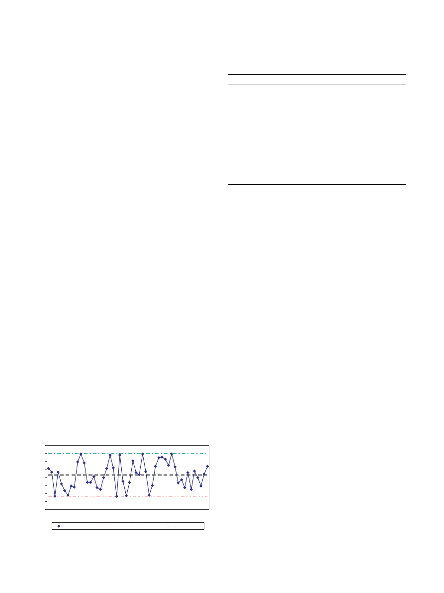
12. Results

In order to perform fatigue analysis, the computer

code was executed 50 times. The estimated blade lifetime
is shown in

Fig. 13

. One can observe that the results are

bounded by 24 and 18.66 years as the upper and lower
limits, while the average is 21.33 years. The correspond-
ing standard deviation of the obtained results is equal to
1.59 years. Since wind patterns in the investigated region
(Manjil) and consequently the applied load on a blade is
never deterministic, proper scatter in the obtained re-
sults implies a proper fatigue modeling.

One of the obtained results was randomly selected

and the progress of fatigue failure was followed step-
by-step to assure performance of code. This is shown
in

Table 9

.

The results prove that damage progress is logical and

the code can model it properly.

13. Conclusion

In this study, the accumulated fatigue damage model

was presented and applied based on CLT. that employs
stiffness degradation as a single measure of damage esti-
mation. Several checks were carried out on the model in
order to assure proper simulation of the damage pro-
gress. All load cases are identified, calculated and evalu-
ated and negligible cases are ignored. By performing
finite element modeling, the critical zone of the blade
is obtained. Fatigue phenomenon is studied in the se-
lected critical zone using accumulated fatigue damage
modeling. Based on a stochastic approach, random load
cases are weighted by their rate-of-occurrence from wind
patterns of the Manjil region. The results are bounded
between 18.66 years and 24 years as lower and upper
limits. Moreover, 1.59 years as the standard deviation
shows a small range of scatter in the range of obtained
results. These results show that presented accumulated
fatigue damage model and the employed stochastic
method are able to simulate the fatigue damage progress
in a wind turbine composite blade. Considering the con-
servative nature of the employed technique, the investi-
gated blade will have 18.66 years in the worse situation
and 24 years in the best situation.

References

[1] Spera DA, editorWind turbine technology. New York: ASME

Press; 1994.

Results of Stochastic Life Estimation

17

18

19

20

21

22

23

24

25

Samples

Life (Year)

Estimated Life

Lower Band

Upper Band

Middle Band

Fig. 13. Predicted lifetime of blade by STOFAT computer code and
for 50 runs.

Table 9
Fatigue failure trend for one obtained result from STOFAT computer
code

Layer no.

Lay-up

Year of failure

1

+45

9.3

2

45

10.6

3

0

13.13

4

0

15.6

5

0

16.3

6

0

17.2

7

0

18.06

8

0

18.66

9

0

18.73

10

0

18.8

11

0

19

12

0

19.2

13

0

19.3

M.M. Shokrieh, R. Rafiee / Composite Structures 74 (2006) 332–342

341

[2] Sutherland HJ. On the fatigue analysis of wind turbines. Sandia

National Laboratories, Albuquerque, New Mexico, June 1999,
SAND99-0089.

[3] Mandel JF, Samborsky DD, Cairns DS. Fatigue of composite

materials and substructures for wind turbine blades. Sandia
National Laboratories, Albuquerque, New Mexico, March 2002,
SAND2002-0771.

[4] DOE/MSU Composite Materials Fatigue Database, February

26, 2003. Sandia National Laboratories, Albuquerque, New
Mexico.

[5] Auto-CAD user manual, Release 2002.
[6] ANSYS Ver. 5.4 User Manual, SAS Co, 1998.
[7] Tsai SW, Hoa SV, Gay D. Composite materials, design and

applications. CRC Press; 2003.

[8] HexPly Data Sheets, M9.6 Series for Wind Turbine Blade

Application, Hexcel Composites Co., France Branch, 2002.

[9] Shokrieh MM, Rafiee R. Extraction of required mechanical

properties for FEM analysis of multidirection composites
using CLT approach. CANCOM, 2005, Vancouver, Canada,
accepted.

[10] Tsai SW, Thomas Hahn H. Introduction to composite materi-

als. USA: Technomic Publishing Co; 1980.

[11] Lloyd G. Rules and regulations. Non-marine technology, Part IV,

Regulation for the certification of wind energy conversion system.
Definition of load cases, Chapter 4, 1993.

[12] Shokrieh MM, Rafiee R. Stochastic analysis of fatigue phenom-

enon in a HAWT composite blade. Sharjah: ICCST; 2004. p.
197–202.

[13] Shokrieh M, Lessard LB. Progressive fatigue damage modeling of

composite materials, Part I: Modeling. J Compos Mater, USA
2000;34(13):1056–80.

[14] Hull D. An Introduction to Composite Materials. Press Syndicate

of the University of Cambridge; 1981.

[15] Ye, Lin. On fatigue damage accumulation and material degrada-

tion in composite materials. Compos Sci Technol 1989;36:339–50.

[16] Shokrieh MM, Zakeri M. Evaluation of fatigue life of composite

materials using progressive damage modeling and stiffness reduc-
tion. In: Proceedings of the 11th annual conference of mechanical
engineering, Iran, Mashhad, 2003. p. 1256–63.

[17] The Mathematica Book, STEPHEN WOLFRAM, 4th ed.,

Mathematica Version 4, 1999.

[18] Charewics A, Daneil IM. Damage mechanics and accumulation in

graphite/epoxy laminates. In: Hahn HT, editor. Composite
materials: fatigue and fracture. ASTM STP 907, 1986. p. 247–97.

[19] Lee JW, Daniel IM, Yaniv G. Fatigue life prediction of cross-ply

composite laminated. In: Lagace PA, editor. Composite materials:
fatigue and fracture. ASTM STP 1012, vol. 2, 1989. p. 19–28.

[20] Shokrieh MM, Rafiee R. Lifetime prediction of HAWT composite

blade. In: 8th international conference of mechanical engineering,
Tehran, 2004. p. 240.

[21] Noda M, Flay RGJ. A simulation model for wind turbine blade

fatigue loads. J Wind Eng Ind Aerodynam 1999;83:527–40.

[22] Eggleston DM, Stoddard FS. Wind turbine engineering

design. New York: Van Nostrand Reinhold; 1978.

[23] Kleiber M, Hien TD. The stochastic finite element method. New

York: John Wiley Publisher Science; 1992.

342

M.M. Shokrieh, R. Rafiee / Composite Structures 74 (2006) 332–342