Numerical linear algebra in data mining

Acta Numerica

(2006), pp. 327–384

Cambridge University Press, 2006

doi: 10.1017/S0962492906240017

Printed in the United Kingdom

Numerical linear algebra in data mining

Lars Eld´

Department of Mathematics,

Link¨

oping University, SE-581 83 Link¨

oping, Sweden

E-mail: laeld@math.liu.se

Ideas and algorithms from numerical linear algebra are important in several
areas of data mining. We give an overview of linear algebra methods in text
mining (information retrieval), pattern recognition (classification of hand-
written digits), and PageRank computations for web search engines. The
emphasis is on rank reduction as a method of extracting information from a
data matrix, low-rank approximation of matrices using the singular value de-
composition and clustering, and on eigenvalue methods for network analysis.

CONTENTS

1 Introduction

327

2 Vectors and matrices in data mining

329

3 Data compression: low-rank approximation

333

4 Text mining

341

5 Classification and pattern recognition

358

6 Eigenvalue methods in data mining

367

7 New directions

377

References

378

1. Introduction

1.1. Data mining

In modern society huge amounts of data are stored in databases with the
purpose of extracting useful information. Often it is not known at the
occasion of collecting the data what information is going to be requested,
and therefore the database is often not designed for the distillation of

328

L. Eld´

any particular information, but rather it is to a large extent unstructured.
The science of extracting useful information from large data sets is usually
referred to as ‘data mining’, sometimes along with ‘knowledge discovery’.

There are numerous application areas of data mining, ranging from

e-business (Berry and Linoff 2000, Mena 1999) to bioinformatics (Bergeron
2002), from scientific application such as astronomy (Burl, Asker, Smyth,
Fayyad, Perona, Crumpler and Aubele 1998), to information retrieval
(Baeza-Yates and Ribeiro-Neto 1999) and Internet search engines (Berry
and Browne 2005).

Data mining is a truly interdisciplinary science, where techniques from

computer science, statistics and data analysis, pattern recognition, linear
algebra and optimization are used, often in a rather eclectic manner. Be-
cause of the practical importance of the applications, there are now numer-
ous books and surveys in the area. We cite a few here: Christianini and
Shawe-Taylor (2000), Cios, Pedrycz and Swiniarski (1998), Duda, Hart and
Storck (2001), Fayyad, Piatetsky-Shapiro, Smyth and Uthurusamy (1996),
Han and Kamber (2001), Hand, Mannila and Smyth (2001), Hastie, Tibshi-
rani and Friedman (2001), Hegland (2001) and Witten and Frank (2000).

The purpose of this paper is not to give a comprehensive treatment of

the areas of data mining, where linear algebra is being used, since that
would be a far too ambitious undertaking. Instead we will present a few
areas in which numerical linear algebra techniques play an important role.
Naturally, the selection of topics is subjective, and reflects the research
interests of the author.

This survey has three themes, as follows.

(1) Information extraction from a data matrix by a rank reduction process.

By determining the ‘principal direction’ of the data, the ‘dominating’

information is extracted first. Then the data matrix is deflated (explicitly
or implicitly) and the same procedure is repeated. This can be formalized
using the Wedderburn rank reduction procedure (Wedderburn 1934), which
is the basis of many matrix factorizations.

The second theme is a variation of the rank reduction idea.

(2) Data compression by low-rank approximation: A data matrix A ∈

×n

, where m and n are large, will be approximated by a rank-k

matrix,

A ≈ W Z

W ∈ R

×k

Z ∈ R

×k

where k ≪ min(m, n).

In many applications the data matrix is huge, and difficult to use for

storage and efficiency reasons. Thus, one evident purpose of compression is
to obtain a representation of the data set that requires less memory than the

Numerical linear algebra in data mining

329

original data set, and that can be manipulated more efficiently. Sometimes
one wishes to obtain a representation that can be interpreted as the ‘main
directions of variation’ of the data, the principal components. This is done by
building the low-rank approximation from the left and right singular vectors
of A that correspond to the largest singular values. In some applications,
e.g., information retrieval (see Section 4) it is possible to obtain better
search results from the compressed representation than from the original
data. There the low-rank approximation also serves as a ‘denoising device’.

(3) Self-referencing definitions that can be formulated mathematically as

eigenvalue and singular value problems.

The most well-known example is the Google PageRank algorithm, which is
based on the notion that the importance of a web page depends on how
many inlinks it has from other important pages.

2. Vectors and matrices in data mining

Often the data are numerical, and the data points can be thought of as
belonging to a high-dimensional vector space. Ensembles of data points can
then be organized as matrices. In such cases it is natural to use concepts
and techniques from linear algebra.

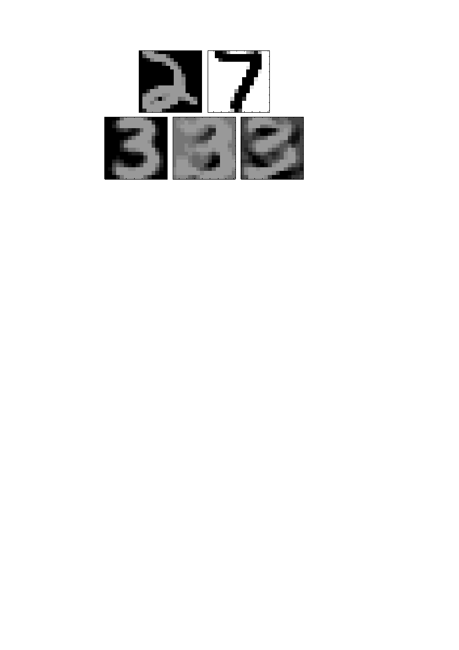
Example 2.1.

Handwritten digit classification is a sub-area of pattern

recognition. Here vectors are used to represent digits. The image of one
digit is a 16 × 16 matrix of numbers, representing grey-scale. It can also be
represented as a vector in R

256

, by stacking the columns of the matrix.

A set of n digits (handwritten 3s, say) can then be represented by matrix

A ∈ R

256×n

, and the columns of A can be thought of as a cluster. They

also span a subspace of R

256

. We can compute an approximate basis of this

subspace using the singular value decomposition (SVD) A = U ΣV

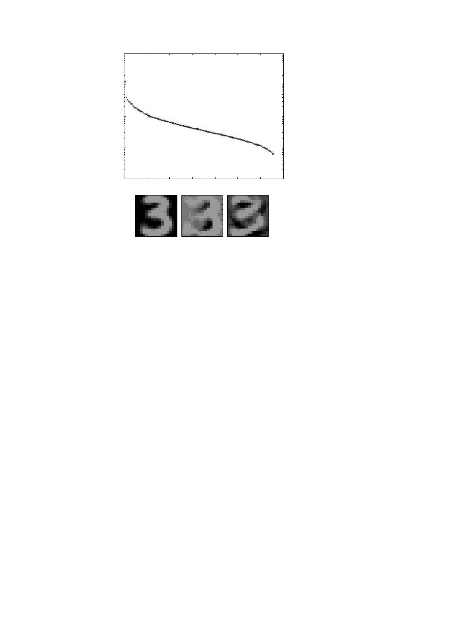
. Three

basis vectors of the ‘3-subspace’ are illustrated in Figure 2.1. The digits are
taken from the US Postal Service database (see, e.g., Hastie et al. (2001)).

Let b be a vector representing an unknown digit, and assume that one

wants to determine, automatically using a computer, which of the digits
0–9 the unknown digit represents. Given a set of basis vectors for 3s,
u

, u

, . . . , u

, we may be able to determine whether b is a 3 or not, by

checking if there is a linear combination of the k basis vectors,

k
j

such that the residual b −

k
j

is small. Thus, we determine the co-

ordinates of b in the basis {u

}

, which is equivalent to solving a least

squares problem with the data matrix U

= (u

. . . u

In Section 5 we discuss methods for classification of handwritten digits.

330

L. Eld´

Figure 2.1. Handwritten digits from the US Postal Service
data base, and basis vectors for 3s (bottom).

It also happens that there is a natural or perhaps clever way of encoding

non-numerical data so that the data points become vectors. We will give
a couple of such examples from text mining (information retrieval) and
Internet search engines.

Example 2.2.

Term-document matrices are used in information retrieval.

Consider the following set of five documents. Key words, referred to as
terms, are marked in boldface.

Document 1:

The Google matrix P is a model of the Internet.

Document 2:

is nonzero if there is a link from web page j to i.

Document 3:

The Google matrix is used to rank all web pages

Document 4:

The ranking is done by solving a matrix eigenvalue
problem.

Document 5:

England dropped out of the top 10 in the FIFA
ranking.

Counting the frequency of terms in each document, we get the result shown
in Table 2.1. The total set of terms is called the dictionary. Each document

To avoid making the example too large, we have ignored some words that would nor-
mally be considered as terms. Note also that only the stem of a word is significant:
‘ranking’ is considered the same as ‘rank’.

Numerical linear algebra in data mining

331

Table 2.1.

Term

Doc. 1

Doc. 2

Doc. 3

Doc. 4

Doc. 5

eigenvalue

England

FIFA

Google

Internet

link

matrix

page

rank

web

is represented by a vector in R

, and we can organize the data as a term-

document matrix,

A =







0 0 0 1 0
0 0 0 0 1
0 0 0 0 1
1 0 1 0 0
1 0 0 0 0
0 1 0 0 0
1 0 1 1 0
0 1 1 0 0
0 0 1 1 1
0 1 1 0 0







∈ R

10×5

Assume that we want to find all documents that are relevant with respect to
the query ‘ranking of web pages’. This is represented by a query vector,
constructed in an analogous way to the term-document matrix, using the
same dictionary,

q =







0
0
0
0
0
0
0
1
1
1







∈ R

332

L. Eld´

- n

Figure 2.2.

Thus the query itself is considered as a document. The information retrieval
task can now be formulated as a mathematical problem: find the columns of
A that are close to the vector q. To solve this problem we use some distance
measure in R

In information retrieval it is common that m is large, of the order 10

say. As most of the documents only contain a small fraction of the terms
in the dictionary, the matrix is sparse.

In some methods for information retrieval, linear algebra techniques (e.g.,

singular value decomposition (SVD)) are used for data compression and
retrieval enhancement. We discuss vector space methods for information
retrieval in Section 4.

The very idea of data mining is to extract useful information from large

and often unstructured sets of data. Therefore it is necessary that the
methods used are efficient and often specially designed for large problems.
In some data mining applications huge matrices occur.

Example 2.3.

The task of extracting information from all the web pages

available on the Internet is performed by search engines. The core of the
Google search engine

is a matrix computation, probably the largest that is

performed routinely (Moler 2002). The Google matrix P is assumed to be
of dimension of the order billions (2005), and it is used as a model of (all)
the web pages on the Internet.

In the Google PageRank algorithm the problem of assigning ranks to all

the web pages is formulated as a matrix eigenvalue problem. Let all web
pages be ordered from 1 to n, and let i be a particular web page. Then O

will denote the set of pages that i is linked to, the outlinks. The number of
outlinks is denoted N

= |O

|. The set of inlinks, denoted I

, are the pages

http://www.google.com

Numerical linear algebra in data mining

333

that have an outlink to i. Now define Q to be a square matrix of dimension
n, and let

1/N

if there is a link from j to i,

otherwise.

This definition means that row i has nonzero elements in those positions
that correspond to inlinks of i. Similarly, column j has nonzero elements
equal to 1/N

in those positions that correspond to the outlinks of j.

The link graph in Figure 2.2 illustrates a set of web pages with outlinks

and inlinks. The corresponding matrix becomes

Q =







1
3

0 0 0

1
3

0 0 0 0

1
3

0 0

1
3

1
2

1
3

0 0 0

1
3

0 0 0

1
2

0 1 0

1
3







Define a vector r, which holds the ranks of all pages. The vector r is then

defined

as the eigenvector corresponding to the eigenvalue λ = 1 of Q:

λr = Qr.

(2.1)

We shall discuss some numerical aspects of the PageRank computation in
Section 6.1.

3. Data compression: low-rank approximation

3.1. Wedderburn rank reduction

One way of measuring the information contents in a data matrix is to com-
pute its rank. Obviously, linearly dependent column or row vectors are
redundant, as they can be replaced by linear combinations of the other, lin-
early independent columns. Therefore, one natural procedure for extracting
information from a data matrix is to systematically determine a sequence of
linearly independent vectors, and deflate the matrix by subtracting rank-one
matrices, one at a time. It turns out that this rank reduction procedure is
closely related to matrix factorization, data compression, dimension reduc-
tion, and feature selection/extraction. The key link between the concepts is
the Wedderburn rank reduction theorem.

This definition is provisional since it does not take into account the mathematical
properties of Q: as the problem is formulated so far, there is usually no unique solution
of the eigenvalue problem.

334

L. Eld´

Theorem 3.1. (Wedderburn 1934)

Suppose A ∈ R

×n

, f ∈ R

×1

and g ∈ R

×1

. Then

rank(A − ω

−1

Af g

A) = rank(A) − 1,

if and only if ω = g

Af = 0.

Based on Theorem 3.1 a stepwise rank reduction procedure can be defined:

Let A

(1)

= A, and define a sequence of matrices {A

(i)

}

(i+1)

= A

(i)

− ω

−1

(i)

(i)T

(i)

(3.1)

for any vectors f

(i)

∈ R

×1

and g

(i)

∈ R

×1

, such that

= g

(i)T

(i)

= 0.

(3.2)

The sequence defined in (3.1) terminates in r = rank(A) steps, since each
time the rank of the matrix decreases by one. This process is called a rank-
reducing process and the matrices A

(i)

are called Wedderburn matrices. For

details, see Chu, Funderlic and Golub (1995). The process gives a matrix
rank-reducing decomposition,

A = ˆ

F Ω

−1

(3.3)

where

F =

, . . . , ˆ

∈ R

×r

= A

(i)

(3.4)

Ω = diag(ω

, . . . , ω

) ∈ R

×r

(3.5)

G =

, . . . , ˆ

∈ R

×r

= A

(i)T

(i)

(3.6)

Theorem 3.1 can be generalized to the case where the reduction of rank is
larger than one, as shown in the next theorem.

Theorem 3.2. (Guttman 1957)

Suppose A ∈ R

×n

, F ∈ R

×k

, and

G ∈ R

×k

. Then

rank(A − AF R

−1

A) = rank(A) − rank(AF R

−1

A),

(3.7)

if and only if R = G

AF ∈ R

×k

is nonsingular.

Chu et al. (1995) discuss Wedderburn rank reduction from the point of

view of solving linear systems of equations. There are many choices of F
and G that satisfy the condition (3.7). Therefore, various rank-reducing
decompositions (3.3) are possible. It is shown that several standard matrix
factorizations in numerical linear algebra are instances of the Wedderburn
formula: Gram–Schmidt orthogonalization, singular value decomposition,
QR and Cholesky decomposition, as well as the Lanczos procedure.

Numerical linear algebra in data mining

335

A complementary view is taken in data analysis

(see Hubert, Meulman

and Heiser (2000)), where the Wedderburn formula and matrix factoriza-
tions are considered as tools for data analysis: ‘The major purpose of a
matrix factorization in this context is to obtain some form of lower-rank ap-
proximation to A for understanding the structure of the data matrix . . . ’.

One important difference in the way the rank reduction is treated in data

analysis and in numerical linear algebra, is that in algorithm descriptions
in data analysis the subtraction of the rank-one matrix ω

−1

Af g

A is often

done explicitly, whereas in numerical linear algebra it is mostly implicit. One
notable example is the Partial Least Squares method (PLS) that is widely
used in chemometrics. PLS is equivalent to Lanczos bidiagonalization: see
Section 3.4. This difference in description is probably the main reason why
the equivalence between PLS and Lanczos bidiagonalization has not been
widely appreciated in either community, even though it was pointed out
quite early (Wold, Ruhe, Wold and Dunn 1984).

The application of the Wedderburn formula to data mining is further

discussed in Park and Eld´en (2005).

3.2. SVD, Eckart–Young optimality, and principal component analysis

We will here give a brief account of the SVD, its optimality properties
for low-rank matrix approximation, and its relation to principal component
analysis (PCA). For a more detailed exposition, see, e.g., Golub and Van
Loan (1996).

Theorem 3.3.

Any matrix A ∈ R

×n

, with m ≥ n, can be factorized

A = U ΣV

Σ =

∈ R

×n

= diag(σ

, . . . , σ

where U ∈ R

×m

and V ∈ R

×n

are orthogonal, and σ

≥ σ

≥ · · · σ

≥ 0.

The assumption m ≥ n is no restriction. The σ

are the singular values,

and the columns of U and V are left and right singular vectors, respectively.

Suppose that A has rank r. Then σ

> 0, σ

= 0, and

A = U ΣV

= U

(3.8)

where U

∈ R

×r

, Σ

= diag(σ

, . . . , σ

) ∈ R

×r

, and V

∈ R

×r

. From (3.8)

It is interesting to note that several of the linear algebra ideas used in data mining were
originally conceived in applied statistics and data analysis, especially in psychometrics.

336

L. Eld´

we see that the columns of U and V provide bases for all four fundamental
subspaces of A:

gives an orthogonal basis for Range(A),

gives an orthogonal basis for Null(A),

gives an orthogonal basis for Range(A

gives an orthogonal basis for Null(A

where Range and Null denote the range space and the null space of the
matrix, respectively.

Often it is convenient to write the SVD in outer product form, i.e., express

the matrix as a sum of rank-one matrices,

A =

(3.9)

The SVD can be used to compute the rank of a matrix. However, in

floating point arithmetic, the zero singular values usually appear as small
numbers. Similarly, if A is made up from a rank-k matrix and additive
noise of small magnitude, then it will have k singular values that will be
significantly larger than the rest. In general, a large relative gap between two
consecutive singular values is considered to reflect numerical rank deficiency
of a matrix. Therefore, ‘noise reduction’ can be achieved via a truncated
SVD. If trailing small diagonal elements of Σ are replaced by zeros, then a
rank-k approximation A

of A is obtained as

A =

≈

= U

=: A

(3.10)

where Σ

∈ R

×k

and ˆ

< ǫ for a small tolerance ǫ.

The low-rank approximation of a matrix obtained in this way from the

SVD has an optimality property specified in the following theorem (Eckart
and Young 1936, Mirsky 1960), which is the foundation of numerous im-
portant procedures in science and engineering. An orthogonally invariant
matrix norm is one, for which QAP = A, where Q and P are arbitrary
orthogonal matrices (of conforming dimensions). The matrix 2-norm and
the Frobenius norm are orthogonally invariant.

Theorem 3.4.

Let · denote any orthogonally invariant norm, and let

the SVD of A ∈ R

×n

be given as in Theorem 3.3. Assume that an integer

k is given with 0 < k ≤ r = rank(A). Then

min

rank(B)=k

A − B = A − A

Numerical linear algebra in data mining

337

where

= U

(3.11)

From the theorem we see that the singular values indicate how close a

given matrix is to a matrix of lower rank.

The relation between the truncated SVD (3.11) and the Wedderburn ma-

trix rank reduction process can be demonstrated as follows. In the rank
reduction formula (3.7), define the error matrix E as

E = A − AF (G

AF )

−1

F ∈ R

×k

, G ∈ R

×k

Assume that k ≤ rank(A) = r, and consider the problem

min E =

min

∈R

n×k

∈R

m×k

A − AF (G

AF )

−1

where the norm is orthogonally invariant. According to Theorem 3.4, the
minimum error is obtained when

(AF )(G

AF )

−1

A) = U

which is equivalent to choosing F = V

and G = U

This same result can be obtained by a stepwise procedure, when k pairs

of vectors f

(i)

and g

(i)

are to be found, where each pair reduces the matrix

rank by 1.

The Wedderburn procedure helps to elucidate the equivalence between the

SVD and principal component analysis (PCA) (Joliffe 1986). Let X ∈ R

×n

be a data matrix, where each column is an observation of a real-valued
random vector. The matrix is assumed to be centred, i.e., the mean of each
column is equal to zero. Let the SVD of X be X = U ΣV

. The right

singular vectors v

are called principal component directions of X (Hastie

et al. 2001, p. 62). The vector

= Xv

= σ

has the largest sample variance amongst all normalized linear combinations
of the columns of X:

Var(z

) = Var(Xv

) =

Finding the vector of maximal variance is equivalent, using linear algebra
terminology, to maximizing the Rayleigh quotient:

= max

= arg max

The normalized variable u

is called the normalized first principal com-

ponent of X. The second principal component is the vector of largest sample

338

L. Eld´

variance of the deflated data matrix X −σ

, and so on. Any subsequent

principal component is defined as the vector of maximal variance subject to
the constraint that it is orthogonal to the previous ones.

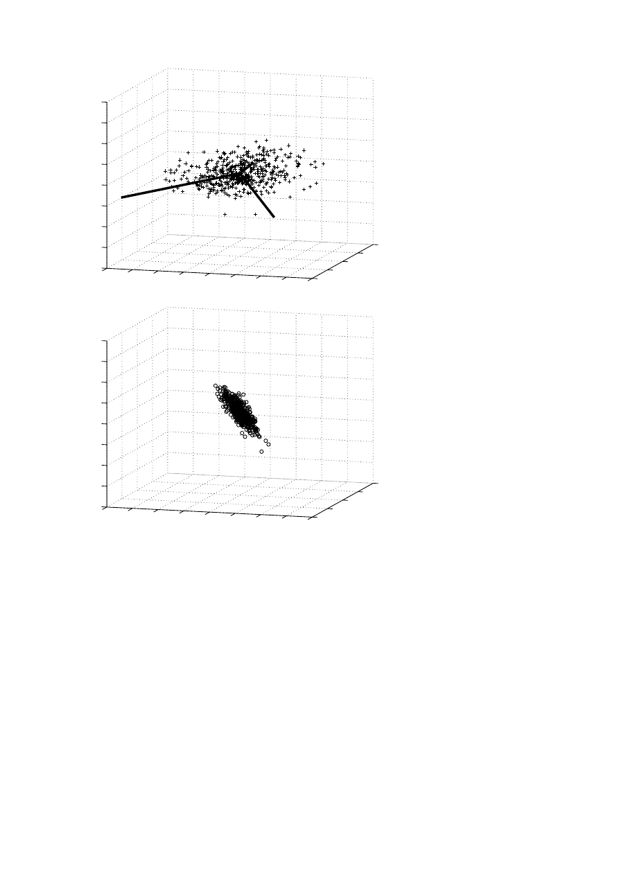
Example 3.5.

PCA is illustrated in Figure 3.1. 500 data points from

a correlated normal distribution were generated, and collected in a data
matrix X ∈ R

3×500

. The data points and the principal components are

illustrated in the top plot. We then deflated the data matrix: X

:= X −

. The data points corresponding to X

are given in the bottom plot;

they lie on a plane in R

, i.e., X

has rank 2.

The concept of principal components has been generalized to principal

curves and surfaces: see Hastie (1984) and Hastie et al. (2001, Section
14.5.2). A recent paper along these lines is Einbeck, Tutz and Evers (2005).

3.3. Generalized SVD

The SVD can be used for low-rank approximation involving one matrix. It
often happens that two matrices are involved in the criterion that determines
the dimension reduction: see Section 4.4. In such cases a generalization of
the SVD to two matrices can be used to analyse and compute the dimension
reduction transformation.

Theorem 3.6. (GSVD)

Let A ∈ R

×n

, m ≥ n, and B ∈ R

×n

. Then

there exist orthogonal matrices U ∈ R

×m

and V ∈ R

×p

, and a nonsingular

X ∈ R

×n

, such that

AX = C = diag(c

, . . . , c

1 ≥ c

≥ · · · ≥ c

≥ 0,

(3.12)

BX = S = diag(s

, . . . , s

0 ≤ s

≤ · · · ≤ s

≤ 1,

(3.13)

where q = min(p, n) and

C + S

S = I.

A proof can be found in Golub and Van Loan (1996, Section 8.7.3); see

also Van Loan (1976) and Paige and Saunders (1981).

The generalized SVD is sometimes called the Quotient SVD.

There is

also a different generalization, called the Product SVD: see, e.g., De Moor
and Van Dooren (1992), Golub, Sølna and Van Dooren (2000).

3.4. Partial least squares: Lanczos bidiagonalization

Linear least squares (regression) problems occur frequently in data mining.
Consider the minimization problem

min

y − Xβ,

(3.14)

Assume that B is square and nonsingular. Then the GSVD gives the SVD of AB

−1

Numerical linear algebra in data mining

339

−1

−2

−3

−4

−1

−2

−3

−4

Figure 3.1. Cluster of points in R

with (scaled) principal

components (top). The same data with the contributions
along the first principal component deflated (bottom).

340

L. Eld´

where X is an m × n real matrix, and the norm is the Euclidean vector
norm. This is the linear least squares problem in numerical linear algebra,
and the multiple linear regression problem in statistics. Using regression ter-
minology, the vector y consists of observations of a response variable, and
the columns of X contain the values of the explanatory variables. Often
the matrix is large and ill-conditioned: the column vectors are (almost) lin-
early dependent. Sometimes, in addition, the problem is under-determined,
i.e., m < n. In such cases the straightforward solution of (3.14) may be
physically meaningless (from the point of view of the application at hand)
and difficult to interpret. Then one may want to express the solution by
projecting it onto a lower-dimensional subspace: let W be an n × k ma-
trix with orthonormal columns. Using this as a basis for the subspace, one
considers the approximate minimization

min

y − Xβ ≈ min

y − XW z.

(3.15)

One obvious method for projecting the solution onto a low-dimensional sub-
space is principal components regression (PCR) (Massy 1965), where the
columns of W are chosen as right singular vectors from the SVD of X. In
numerical linear algebra this is called truncated singular value decomposition
(TSVD). Another such projection method, the partial least squares (PLS)
method (Wold 1975), is standard in chemometrics (Wold, Sj¨

ostr¨om and

Eriksson 2001). It has been known for quite some time (Wold et al. 1984)
(see also Helland (1988), Di Ruscio (2000), Phatak and de Hoog (2002))
that PLS is equivalent to Lanczos (Golub–Kahan) bidiagonalization (Golub
and Kahan 1965, Paige and Saunders 1982) (we will refer to this as LBD).
The equivalence is further discussed in Eld´en (2004b), and the properties of
PLS are analysed using the SVD.

There are several variants of PLS: see, e.g., Frank and Friedman (1993).

The following is the so-called NIPALS version.

The NIPALS PLS algorithm

1 X

= X

2 for i = 1, 2, . . . , k

(a) w

i−1

−1

(b) t

i−1

−1

= X

−1

(d) X

= X

−1

− t

In the statistics/chemometrics literature the vectors w

, t

, and p

are

called weight, score, and loading vectors, respectively.

Numerical linear algebra in data mining

341

It is obvious that PLS is a Wedderburn procedure. One advantage of PLS

for regression is that the basis vectors in the solution space (the columns
of W (3.15)) are influenced by the right-hand side.

This is not the case in

PCR, where the basis vectors are singular vectors of X. Often PLS gives a
higher reduction of the norm of the residual y − Xβ for small values of k
than does PCR.

The Lanczos bidiagonalization procedure can be started in different ways:

see, e.g., Bj¨

orck (1996, Section 7.6). It turns out that PLS corresponds to

the following formulation.

Lanczos Bidiagonalization (LBD)

1 v

= Xv

2 for i = 2, . . . , k

(a) γ

−1

= X

−1

− α

−1

(b) α

= Xv

− γ

−1

The coefficients γ

−1

and α

are determined so that v

= u

= 1.

Both algorithms generate two sets of orthogonal basis vectors: (w

)

and

)

for PLS, (v

)

and (u

)

for LBD. It is straightforward to show

(directly using the equations defining the algorithm – see Eld´en (2004b))
that the two methods are equivalent.

Proposition 3.7.

The PLS and LBD methods generate the same orthog-

onal bases, and the same approximate solution, β

(k)

pls

= β

(k)

lbd

4. Text mining

By text mining we understand methods for extracting useful information
from large and often unstructured collections of texts. A related term is in-
formation retrieval. A typical application is search in databases of abstract
of scientific papers. For instance, in medical applications one may want to
find all the abstracts in the database that deal with a particular syndrome.
So one puts together a search phrase, a query, with key words that are rele-
vant to the syndrome. Then the retrieval system is used to match the query
to the documents in the database, and present to the user all the documents
that are relevant, preferably ranked according to relevance.

However, it is not always appreciated that the dependence of the basis vectors on the
right-hand side is non-linear and quite complicated. For a discussion of these aspects
of PLS, see Eld´en (2004b).

342

L. Eld´

Example 4.1.

The following is a typical query:

9. the use of induced hypothermia in heart surgery, neurosurgery, head injuries and
infectious diseases.

The query is taken from a test collection of medical abstracts, called Med-
line.

We will refer to this query as Q9 from here on.

Another well-known area of text mining is web search engines. There the

search phrase is usually very short, and often there are so many relevant
documents that it is out of the question to present them all to the user. In
that application the ranking of the search result is critical for the efficiency
of the search engine. We will come back to this problem in Section 6.1.

For overviews of information retrieval, see, e.g., Korfhage (1997) and

Grossman and Frieder (1998). In this section we will describe briefly one of
the most common methods for text mining, namely the vector space model
(Salton, Yang and Wong 1975). In Example 2.2 we demonstrated the basic
ideas of the construction of a term-document matrix in the vector space
model. Below we first give a very brief overview of the preprocessing that
is usually done before the actual term-document matrix is set up. Then we
describe a variant of the vector space model: latent semantic indexing (LSI)
(Deerwester, Dumais, Furnas, Landauer and Harsman 1990), which is based
on the SVD of the term-document matrix. For a more detailed account of
the different techniques used in connection with the vector space model, see
Berry and Browne (2005).

4.1. Vector space model: preprocessing and query matching

In information retrieval, key words that carry information about the con-
tents of a document are called terms. A basic task is to create a list of all
the terms in alphabetic order, a so-called index. But before the index is
made, two preprocessing steps should be done: (1) eliminate all stop words,
(2) perform stemming.

Stop words are extremely common words. The occurrence of such a word

in a document does not distinguish it from other documents. The following
is the beginning of one stop list:

a, a’s, able, about, above, according, accordingly, across, actually, after, afterwards,
again, against, ain’t, all, allow, allows, almost, alone, along, already, also, although,
always, am, among, amongst, an, and, . . .

See, e.g., http://www.dcs.gla.ac.uk/idom/ir-resources/test-collections/

ftp://ftp.cs.cornell.edu/pub/smart/english.stop

Numerical linear algebra in data mining

343

Stemming is the process of reducing each word that is conjugated or has

a suffix to its stem. Clearly, from the point of view of information retrieval,
no information is lost in the following reduction:

computable

computation

computing

computed

computational











−→

comput

Public domain stemming algorithms are available on the Internet.

A number of pre-processed documents are parsed,

giving a term-docu-

ment matrix A ∈ R

×n

, where m is the number of terms in the dictionary

and n is the number of documents. It is common not only to count the oc-
currence of terms in documents but also to apply a term-weighting scheme,
where the elements of A are weighted depending on the characteristics of the
document collection. Similarly, document weighting is usually done. A num-
ber of schemes are described in Berry and Browne (2005, Section 3.2.1). For
example, one can define the elements in A by

= f

log(n/n

(4.1)

where f

is the term frequency, the number of times term i appears in

document j, and n

is the number of documents that contain term i (inverse

document frequency). If a term occurs frequently in only a few documents,
then both factors are large. In this case the term discriminates well between
different groups of documents, and it gets a large weight in the documents
where it appears.

Normally, the term-document matrix is sparse: most of the matrix ele-

ments are equal to zero. Then, of course, one avoids storing all the zeros,
and instead uses a sparse matrix storage scheme (see, e.g., Saad (2003,
Chapter 3) and Goharian, Jain and Sun (2003)).

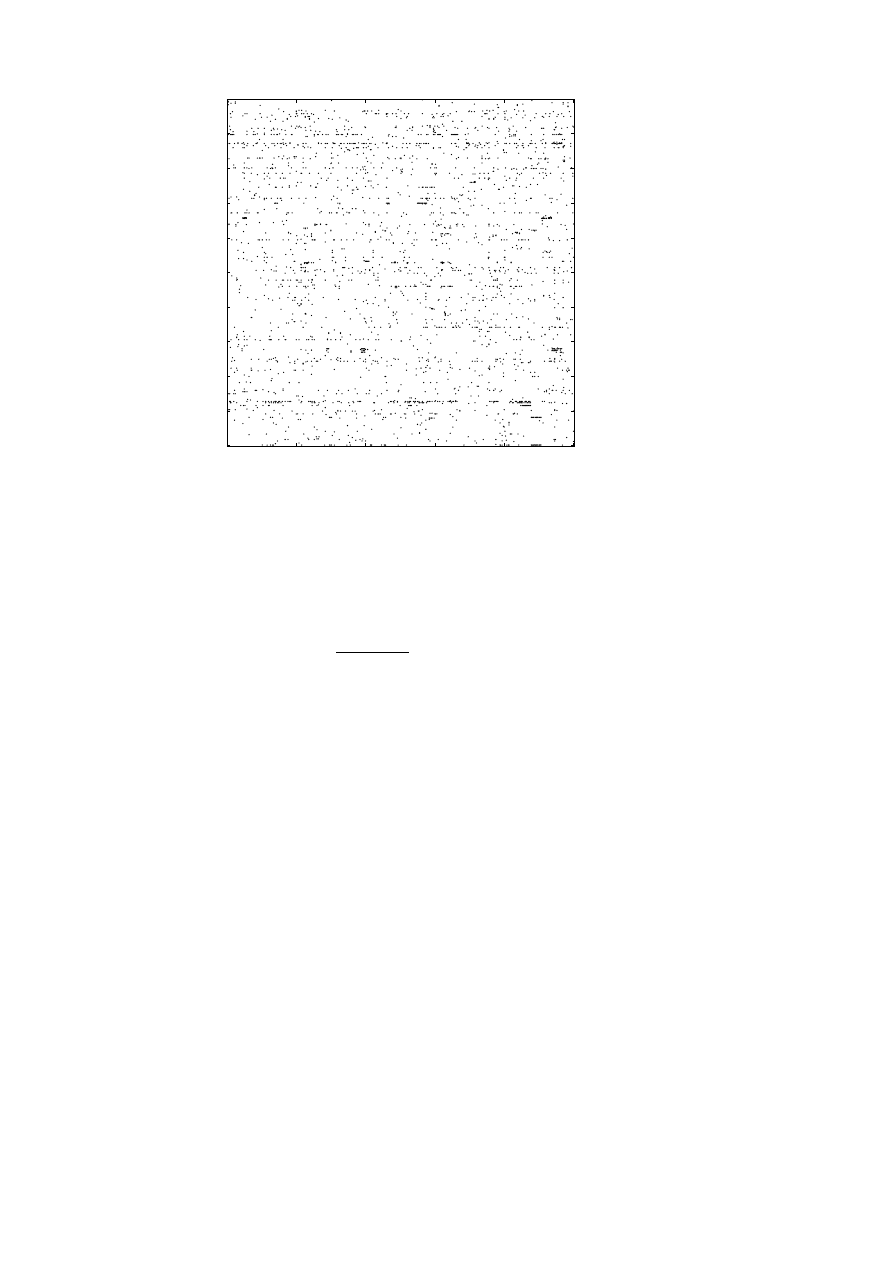
Example 4.2.

For the stemmed Medline collection (cf. Example 4.1) the

matrix (including 30 query columns) is 4163 × 1063 with 48263 nonzero
elements, i.e., approximately 1%. The first 500 rows and columns of the
matrix are illustrated in Figure 4.1.

The query (cf. Example 4.1) is parsed using the same dictionary as the

documents, giving a vector q ∈ R

. Query matching is the process of finding

http://www.tartarus.org/~martin/PorterStemmer/.

Public domain text parsers are described in Giles, Wo and Berry (2003) and Zeimpekis
and Gallopoulos (2005).

344

L. Eld´

100

150

200

250

300

350

400

450

500

nz = 2685

Figure 4.1. The first 500 rows and columns of the Medline
matrix. Each dot represents a nonzero element.

all documents that are considered relevant to a particular query q. This is
often done using the cosine distance measure: all documents are returned
for which

> tol,

(4.2)

where tol is a predefined tolerance. If the tolerance is lowered, then more
documents are returned, and then it is likely that more of the documents
that are relevant to the query are returned. But at the same time there is
a risk that more documents that are not relevant are also returned.

Example 4.3.

We did query matching for query Q9 in the stemmed Med-

line collection. With tol = 0.19 only document 409 was considered relevant.
When the tolerance was lowered to 0.17, then documents 409, 415, and 467
were retrieved.

We illustrate the different categories of documents in a query matching

for two values of the tolerance in Figure 4.2. The query matching produces
a good result when the intersection between the two sets of returned and

Numerical linear algebra in data mining

345

RELEVANT

DOCUMENTS

RETURNED

ALL DOCUMENTS

Figure 4.2. Returned and relevant documents for two
values of the tolerance. The dashed circle represents
the returned documents for a high value of the cosine
tolerance.

relevant documents is as large as possible, and the number of returned
irrelevant documents is small. For a high value of the tolerance, the retrieved
documents are likely to be relevant (the small circle in Figure 4.2). When
the cosine tolerance is lowered, then the intersection is increased, but at the
same time, more irrelevant documents are returned.

In performance modelling for information retrieval we define the following

measures:

precision

P =

where D

is the number of relevant documents retrieved, and D

the total

number of documents retrieved; and

recall

R =

where N

is the total number of relevant documents in the data base. With

the cosine measure, we see that with a large value of tol we have high
precision, but low recall. For a small value of tol we have high recall, but
low precision.

In the evaluation of different methods and models for information retrieval

usually a number of queries are used. For testing purposes all documents
have been read by a human and those that are relevant to a certain query
are marked.

346

L. Eld´

100

RECALL (%)

PRECISION

(%)

Figure 4.3. Query matching for Q9 using the
vector space method. Recall versus precision.

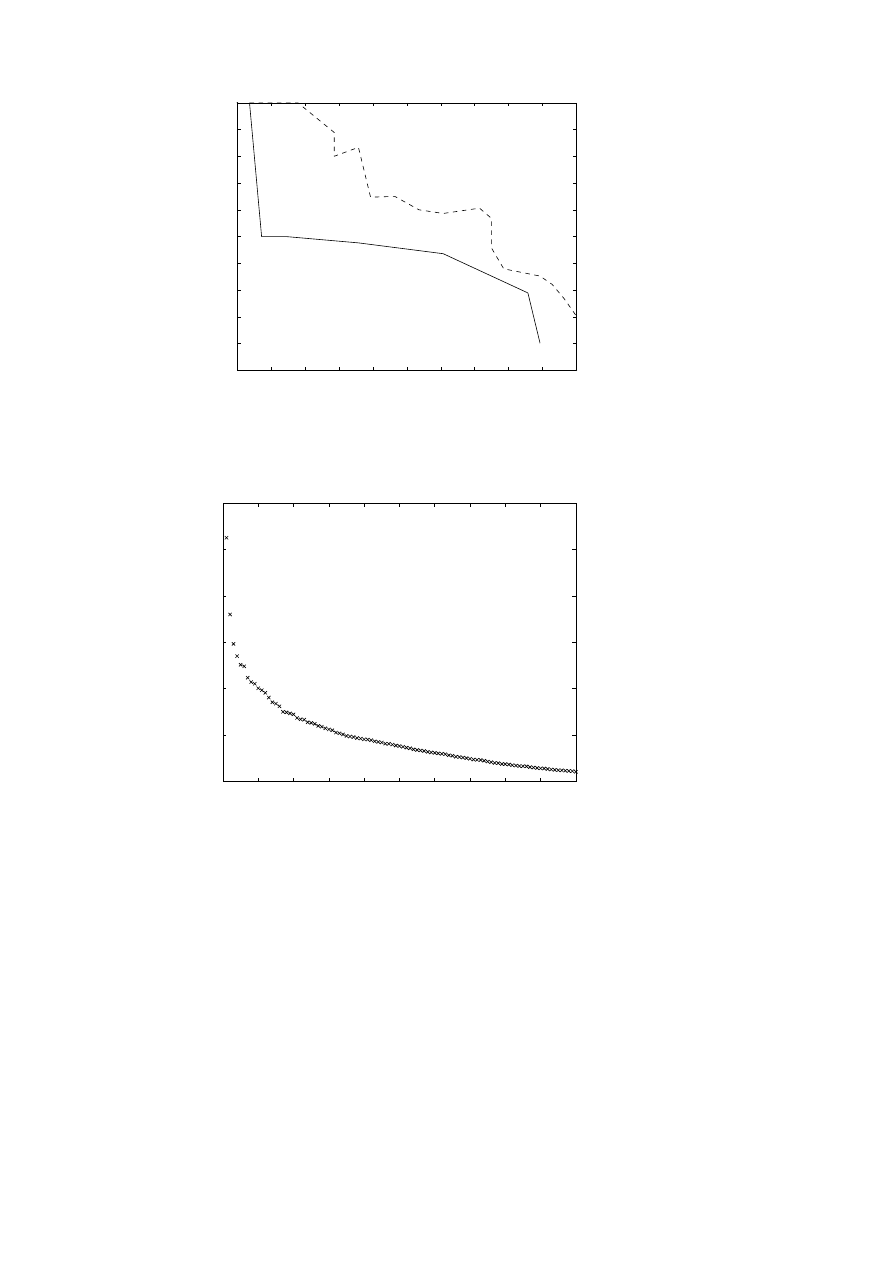
Example 4.4.

We did query matching for query Q9 in the Medline collec-

tion (stemmed) using the cosine measure, and obtained recall and precision
as illustrated in Figure 4.3. In the comparison of different methods it is more
illustrative to draw the recall versus precision diagram. Ideally a method
has high recall at the same time as the precision is high. Thus, the closer
the curve is to the upper right corner, the better the method.

In this example and the following examples the matrix elements were

computed using term frequency and inverse document frequency weight-
ing (4.1).

4.2. LSI: latent semantic indexing

Latent semantic indexing

(LSI) ‘is based on the assumption that there is

some underlying latent semantic structure in the data . . . that is corrupted
by the wide variety of words used . . . ’ (quoted from Park, Jeon and Rosen
(2001)) and that this semantic structure can be enhanced by projecting the
data (the term-document matrix and the queries) onto a lower-dimensional
space using the singular value decomposition. LSI is discussed in Deerwester
et al. (1990), Berry, Dumais and O’Brien (1995), Berry, Drmac and Jessup
(1999), Berry (2001), Jessup and Martin (2001) and Berry and Browne
(2005).

Sometimes also called latent semantic analysis (LSA) (Jessup and Martin 2001).

Numerical linear algebra in data mining

347

Let A = U ΣV

be the SVD of the term-document matrix and approxi-

mate it by a matrix of rank k:

≈

= U

(Σ

) =: U

The columns of U

live in the document space and are an orthogonal ba-

sis that we use to approximate all the documents: column j of D

holds

the coordinates of document j in terms of the orthogonal basis. With
this k-dimensional approximation the term-document matrix is represented
by A

= U

, and in query matching we compute q

= q

. Thus, we compute the coordinates of the query in terms of the

new document basis and compute the cosines from

cos θ

)

= U

(4.3)

This means that the query matching is performed in a k-dimensional space.

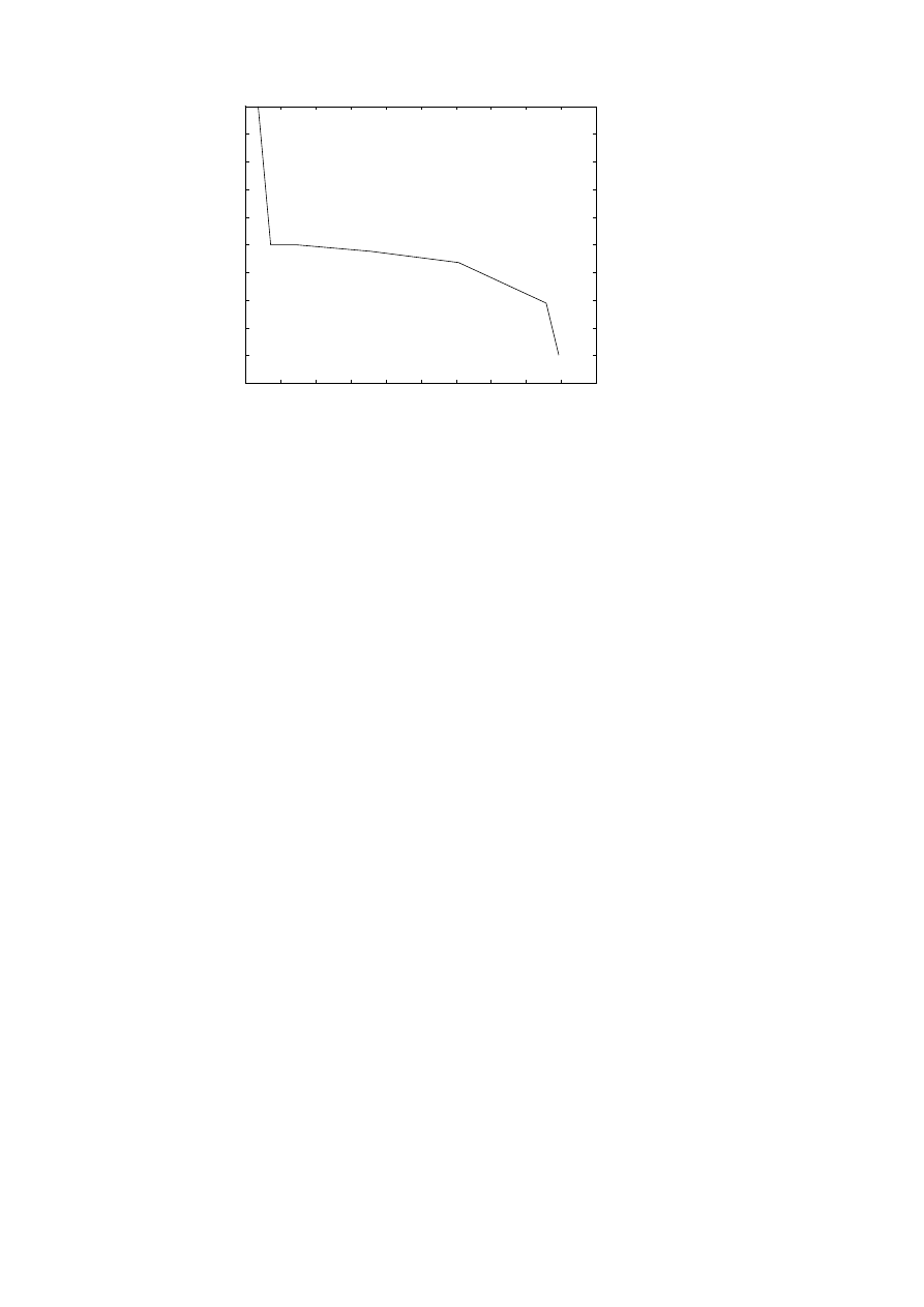
Example 4.5.

We did query matching for Q9 in the Medline collection,

approximating the matrix using the truncated SVD of rank 100. The recall–
precision curve is given in Figure 4.4. It is seen that for this query LSI
improves the retrieval performance. In Figure 4.5 we also demonstrate a
fact that is common to many term-document matrices: it is rather well con-
ditioned, and there is no gap in the sequence of singular values. Therefore,
we cannot find a suitable rank of the LSI approximation by inspecting the
singular values: it must be determined by retrieval experiments.

Another remarkable fact is that with k = 100 the approximation error in

the matrix approximation,

A − A

≈ 0.8,

is large, and we still get improved retrieval performance. In view of the
large approximation error in the truncated SVD approximation of the term-
document matrix, one may question whether the ‘optimal’ singular vectors
constitute the best basis for representing the term-document matrix. On
the other hand, since we get such good results, perhaps a more natural
conclusion may be that the Frobenius norm is not a good measure of the
information contents in the term-document matrix.

348

L. Eld´

100

RECALL (%)

PRECISION

(%)

Figure 4.4. Query matching for Q9. Recall versus
precision for the full vector space model (solid
line) and the rank-100 approximation (dashed).

100

150

200

250

300

350

400

Figure 4.5. First 100 singular values
of the Medline (stemmed) matrix.

Numerical linear algebra in data mining

349

It is also interesting to see what are the most important ‘directions’ in

the data. From Theorem 3.4 we know that the first few left singular vec-
tors are the dominant directions in the document space, and their largest
components should indicate what these directions are. The Matlab state-
ments find(abs(U(:,k))>0.13), combined with look-up in the dictionary
of terms, gave the results shown in Table 4.1, for k=1,2.

Table 4.1.

U(:,1)

U(:,2)

cell

case

growth

cell

hormone

children

patient

defect
dna
growth
patient
ventricular

It should be said that LSI does not give significantly better results for all

queries in the Medline collection: there are some where it gives results com-
parable to the full vector model, and some where it gives worse performance.
However, it is often the average performance that matters.

Jessup and Martin (2001) made a systematic study of different aspects of

LSI. They showed that LSI improves retrieval performance for surprisingly
small values of the reduced rank k. At the same time the relative matrix
approximation errors are large. It is probably not possible to prove any
general results for LSI that explain how and for which data it can improve
retrieval performance. Instead we give an artificial example (constructed
using ideas similar to those of a corresponding example in Berry and Browne
(2005)) that gives a partial explanation.

Example 4.6.

Consider the term-document matrix from Example 2.2,

and the query ‘ranking of web pages’. Obviously, Documents 1–4 are
relevant with respect to the query, while Document 5 is totally irrelevant.
However, we obtain the following cosines for query and the original data:

0 0.6667 0.7746 0.3333 0.3333

We then compute the SVD of the term-document matrix, and use a rank-
two approximation. After projection to the two-dimensional subspace the

350

L. Eld´

0.5

−0

−1

0.8

1.2

1.4

1.6

1.8

2.2

Figure 4.6. The documents and the query projected to
the coordinate system of the first two left singular vectors.

cosines, computed according to (4.3), are

0.7857 0.8332 0.9670 0.4873 0.1819

It turns out that Document 1, which was deemed totally irrelevant to the
query in the original representation, is now highly relevant. In addition,
the scores for the relevant Documents 2–4 have been reinforced. At the
same time, the score for Document 5 has been significantly reduced. Thus,
in this artificial example, the dimension reduction enhanced the retrieval
performance. The improvement may be explained as follows.

In Figure 4.6 we plot the five documents and the query in the coordinate

system of the first two left singular vectors. Obviously, in this representa-
tion, the first document is is closer to the query than Document 5. The first
two left singular vectors are







0.1425
0.0787
0.0787
0.3924
0.1297
0.1020
0.5348
0.3647
0.4838
0.3647













0.2430
0.2607
0.2607

−0.0274

0.0740

−0.3735

0.2156

−0.4749

0.4023

−0.4749







Numerical linear algebra in data mining

351

and the singular values are Σ = diag(2.8546, 1.8823, 1.7321, 1.2603, 0.8483).
The first four columns in A are strongly coupled via the words Google,
matrix, etc., and those words are the dominating contents of the document
collection (cf. the singular values). This shows in the composition of u

So even if none of the words in the query is matched by Document 1, that
document is so strongly correlated to the the dominating direction that it
becomes relevant in the reduced representation.

4.3. Clustering and least squares

Clustering is widely used in pattern recognition and data mining. We give
here a brief account of the application of clustering to text mining.

Clustering is the grouping together of similar objects. In the vector space

model for text mining, similarity is defined as the distance between points
in R

, where m is the number of terms in the dictionary. There are many

clustering methods, e.g., the k-means method, agglomerative clustering,
self-organizing maps, and multi-dimensional scaling: see the references in
Dhillon (2001), Dhillon, Fan and Guan (2001).

The relation between the SVD and clustering is explored in Dhillon (2001);

see also Zha, Ding, Gu, He and Simon (2002) and Dhillon, Guan and Kulis
(2005). Here the approach is graph-theoretic. The sparse term-document
matrix represents a bi-partite graph, where the two sets of vertices are the
documents {d

} and the terms {t

}. An edge (t

, d

) exists if term t

occurs

in document d

, i.e., if the element in position (i, j) is nonzero. Clustering

the documents is then equivalent to partitioning the graph. A spectral par-
titioning method is described, where the eigenvectors of a Laplacian of the
graph are optimal partitioning vectors. Equivalently, the singular vectors of
a related matrix can be used. It is of some interest that spectral clustering
methods are related to algorithms for the partitioning of meshes in parallel
finite element computations: see, e.g., Simon, Sohn and Biswas (1998).

Clustering for text mining is discussed in Dhillon and Modha (2001) and

Park, Jeon and Rosen (2003), and the similarities between LSI and cluster-
ing are pointed out in Dhillon and Modha (2001).

Given a partitioning of a term-document matrix into k clusters,

A =

· · · A

(4.4)

where A

∈ R

, one can take the centroid of each cluster,

(j)

1 1 · · · 1

(4.5)

with e

(j)

∈ R

, as a representative of the class. Together the centroid

In Dhillon and Modha (2001) normalized centroids are called concept vectors.

352

L. Eld´

100

RECALL (%)

PRECISION

(%)

Figure 4.7. Query matching for Q9. Recall versus
precision for the full vector space model (solid line)
and the rank-50 centroid approximation (dashed).

vectors can be used as an approximate basis for the document collection,
and the coordinates of each document with respect to this basis can be
computed by solving the least squares problem

min

A − CD

C =

(1)

(2)

· · · c

(k)

(4.6)

Example 4.7.

We did query matching for Q9 in the Medline collection.

Before computing the clustering we normalized the columns to equal Eu-
clidean length. We approximated the matrix using the orthonormalized
centroids from a clustering into 50 clusters. The recall–precision diagram
is given in Figure 4.7. We see that for high values of recall, the centroid
method is as good as the LSI method with double the rank: see Figure 4.4.

For rank 50 the approximation error in the centroid method,

A − CD

≈ 0.9,

is even higher than for LSI of rank 100.

The improved performance can be explained in a similar way as for LSI.

Being the ‘average document’ of a cluster, the centroid captures the main
links between the dominant documents in the cluster. By expressing all
documents in terms of the centroids, the dominant links are emphasized.

Numerical linear algebra in data mining

353

4.4. Clustering and linear discriminant analysis

When centroids are used as basis vectors, the coordinates of the documents
are computed from (4.6) as

D := G

= R

−1

where C = QR is the thin QR decomposition

of the centroid matrix.

The criterion for choosing G is based on approximating the term-document
matrix A as well as possible in the Frobenius norm. As we have seen earlier
(Examples 4.5 and 4.7), a good approximation of A is not always necessary
for good retrieval performance, and it may be natural to look for other
criteria for determining the matrix G in a dimension reduction.

Linear discriminant analysis (LDA) is frequently used for classification

(Duda et al. 2001). In the context of cluster-based text mining, LDA is
used to derive a transformation G, such that the cluster structure is as well
preserved as possible in the dimension reduction.

In Howland, Jeon and Park (2003) and Howland and Park (2004) the ap-

plication of LDA to text mining is explored, and it is shown how the GSVD
(Theorem 3.6) can be used to extend the dimension reduction procedure to
cases where the standard LDA criterion is not valid.

Assume that a clustering of the documents has been made as in (4.4) with

centroids (4.5). Define the overall centroid

c = Ae,

e =

√

1 1 · · · 1

the three matrices

×n

∋ H

− c

(1)

(1)T

− c

(2)

(2)T

. . . A

− c

(k)

(k)T

×k

∋ H

√

(1)

− c)

√

(2)

− c) . . .

√

(k)

− c)

×n

∋ H

= A − c e

and the corresponding scatter matrices

= H

Assume that we want to use the (dimension-reduced) clustering for clas-
sifying new documents, i.e., determine to which cluster they belong. The
‘quality of the clustering’ with respect to this task depends on how ‘tight’

The thin QR decomposition of a matrix A ∈ R

m×n

, with m ≥ n, is A = QR, where

Q ∈ R

m×n

has orthonormal columns and R is upper triangular.

Note: subscript w for ‘within classes’, b for ‘between classes’.

354

L. Eld´

or coherent each cluster is, and how well separated the clusters are. The
overall tightness (‘within-class scatter’) of the clustering can be measured as

= tr(S

) = H

and the separateness (‘between-class scatter’) of the clusters by

= tr(S

) = H

Ideally, the clusters should be separated at the same time as each cluster is
tight. Different quality measures can be defined. Often in LDA one uses

J =

tr(S

)

tr(S

)

(4.7)

with the motivation that if all the clusters are tight then S

is small, and

if the clusters are well separated then S

is large. Thus the quality of the

clustering with respect to classification is high if J is large. Similar measures
are considered in Howland and Park (2004).

Now assume that we want to determine a dimension reduction transfor-

mation, represented by the matrix G ∈ R

×d

, such that the quality of the

reduced representation is as high as possible. After the dimension reduction,
the tightness and separateness are

(G) = G

= tr(G

G),

(G) = G

= tr(G

G).

Since rank(H

) ≤ k − 1, it is only meaningful to choose d = k − 1: see

Howland et al. (2003).

The question arises whether it is possible to determine G so that, in a

consistent way, the quotient J

(G)/J

(G) is maximized. The answer is

derived using the GSVD of H

and H

. We assume that m > n; see

Howland et al. (2003) for a treatment of the general (but with respect to
the text mining application more restrictive) case. We further assume

rank

= t.

Under these assumptions the GSVD has the form (Paige and Saunders 1981)

= U

(Z 0)Q

(4.8)

= V

(Z 0)Q

(4.9)

where U and V are orthogonal, Z ∈ R

×t

is nonsingular, and Q ∈ R

×m

orthogonal. The diagonal matrices Σ

and Σ

will be specified shortly. We

first see that, with

G = Q

G =

∈ R

×d

Numerical linear algebra in data mining

355

we have

(G) = Σ

(4.10)

Obviously, we should not waste the degrees of freedom in G by choosing a
nonzero

, since that would not affect the quality of the clustering after

dimension reduction. Next we specify

(k−1)×t

∋ Σ







,

×t

∋ Σ







,

where I

∈ R

(t−s)×(t−s)

and I

∈ R

×r

are identity matrices with data-

dependent values of r and s, and 0

∈ R

1×r

and 0

∈ R

(n−s)×(t−s)

are zero

matrices. The diagonal matrices satisfy

= diag(α

, . . . , α

≥ · · · ≥ α

> 0,

(4.11)

= diag(β

, . . . , β

0 < β

≤ · · · ≤ β

(4.12)

and α

+β

= 1, i = r+1, . . . , r+s. Note that the column-wise partitionings

of Σ

and Σ

are identical. Now we define

G = Z







,

where the partitioning conforms with that of Σ

and Σ

. Then we have

(G) = Σ

+ D

(G) = Σ

= D

At this point we see that the maximization of

(G)

tr(

T
b

tr(

(4.13)

is not a well-defined problem: We can make J

(G) large simply by choosing

large, without changing J

(G). On the other hand, (4.13) can be con-

sidered as the Rayleigh quotient of a generalized eigenvalue problem (see,
e.g., Golub and Van Loan (1996, Section 8.7.2)), where the largest set of
eigenvalues are infinite (since the first eigenvalues of Σ

T
b

and Σ

are 1

and 0, respectively), and the following are α

/β

, i = 1, 2, . . . , s. With

this in mind it is natural to constrain the data of the problem so that

G = I.

(4.14)

356

L. Eld´

We see that, under this constraint,

G =

I
0

(4.15)

is a (non-unique) solution of the maximization of (4.13). Consequently, the
transformation matrix G is chosen as

G = Q

−1

= Q

where Y

denotes the first k − 1 columns of Z

−1

LDA-based dimension reduction was tested in Howland et al. (2003) on

data (abstracts) from the Medline database. Classification results were
obtained for the compressed data, with much better precision than using
the full vector space model.

4.5. Text mining using Lanczos bidiagonalization (PLS)

In LSI and cluster-based methods, the dimension reduction is determined
completely from the term-document matrix, and therefore it is the same
for all query vectors. In chemometrics it has been known for a long time
that PLS (Lanczos bidiagonalization) often gives considerably more efficient
compression (in terms of the dimensions of the subspaces used) than PCA
(LSI/SVD), the reason being that the right-hand side (of the least squares
problem) determines the choice of basis vectors.

In a series of papers (see Blom and Ruhe (2005)), the use of Lanczos

bidiagonalization for text mining has been investigated. The recursion starts
with the normalized query vector and computes two orthonormal bases

and Q.

Lanczos Bidiagonalization

1 q

= q/q

= 0,

= 0.

2 for i = 2, . . . , k

(a) α

= A

− β

−1

(b) β

= Apk − α

The coefficients α

and β

are determined so that p

= q

= 1.

We use a slightly different notation here to emphasize that the starting vector is dif-
ferent from that in Section 3.4.

Numerical linear algebra in data mining

357

Define the matrices

· · · q

· · · p

+1,i







. .. α







The recursion can be formulated as matrix equations,

= P

i,i

= Q

+1,i

(4.16)

If we compute the thin QR decomposition of B

+1,i

= H

+1,i+1

then we can write (4.16)

= W

= Q

+1,i+1

which means that the columns of W

are an approximate orthogonal basis

of the document space (cf. the corresponding equation AV

= U

for the

LSI approximation, where we use the columns of U

as basis vectors). Thus

we have

A ≈ W

= W

(4.17)

and we can use this low-rank approximation in the same way as in the LSI
method.

The convergence of the recursion can be monitored by computing the

residual AP

z − q

. It is easy to show (see, e.g., Blom and Ruhe (2005))

that this quantity is equal in magnitude to a certain element in the matrix
H

+1,i+1

. When the residual is smaller than a prescribed tolerance, the

approximation (4.17) is deemed good enough for this particular query.

In this approach the matrix approximation is recomputed for every query.

This has the following advantages.

(1) Since the right-hand side influences the choice of basis vectors, only

a very few steps of the bidiagonalization algorithm need be taken.
Blom and Ruhe (2005) report tests for which this algorithm performed
better, with k = 3, than LSI with subspace dimension 259.

(2) The computation is relatively cheap, the dominating cost being a small

number of matrix-vector multiplications.

358

L. Eld´

(3) Most information retrieval systems change with time, when new docu-

ments are added. In LSI this necessitates the updating of the SVD of
the term-document matrix. Unfortunately, it is quite expensive to up-
date an SVD. The Lanczos-based method, on the other hand, adapts
immediately and at no extra cost to changes of A.

5. Classification and pattern recognition

5.1. Classification of handwritten digits using SVD bases

Computer classification of handwritten digits is a standard problem in pat-
tern recognition. The typical application is automatic reading of zip codes
on envelopes. A comprehensive review of different algorithms is given in
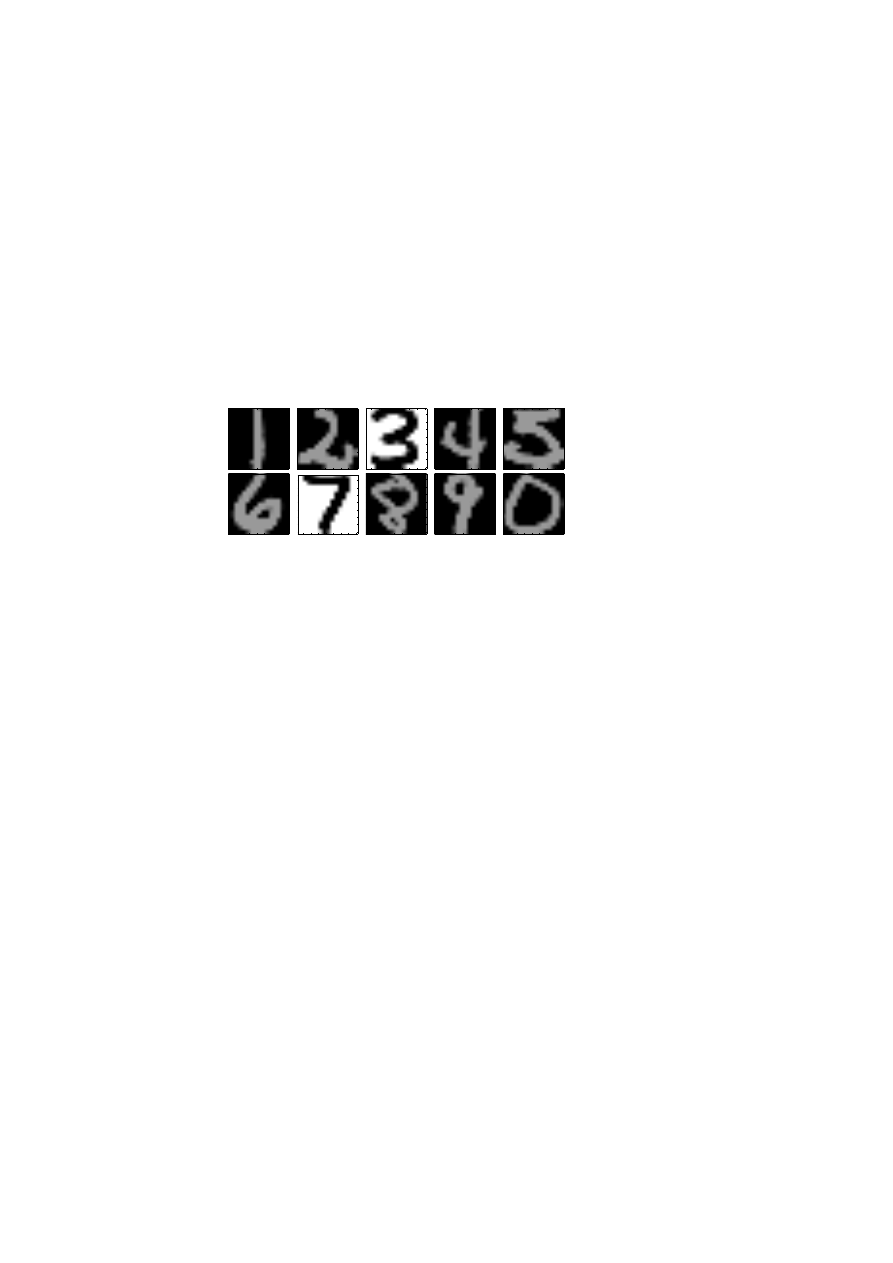
LeCun, Bottou, Bengio and Haffner (1998).

Figure 5.1. Handwritten digits from
the US Postal Service database.

In Figure 5.1 we illustrate handwritten digits that we will use in the

examples in this section.

We will treat the digits in three different, but equivalent ways:

(1) 16 × 16 grey-scale images,
(2) functions of two variables,

(3) vectors in R

256

In the classification of an unknown digit it is necessary to compute the

distance to known digits. Different distance measures can be used, perhaps
the most natural is Euclidean distance: stack the columns of the image in a
vector and identify each digit as a vector in R

256

. Then define the distance

function

dist(x, y) = x − y

Numerical linear algebra in data mining

359

An alternative distance function can be based on the cosine between two
vectors.

In a real application of recognition of handwritten digits, e.g., zip code

reading, there are hardware and real time factors that must be taken into
account. In this section we will describe an idealized setting. The problem is:

Given a set of of manually classified digits (the training set), classify a set of
unknown digits (the test set).

In the US Postal Service database, the training set contains 7291 handwrit-
ten digits, and the test set has 2007 digits.

When we consider the training set digits as vectors or points, then it is

reasonable to assume that all digits of one kind form a cluster of points in a
Euclidean 256-dimensional vector space. Ideally the clusters are well sepa-
rated and the separation depends on how well written the training digits are.

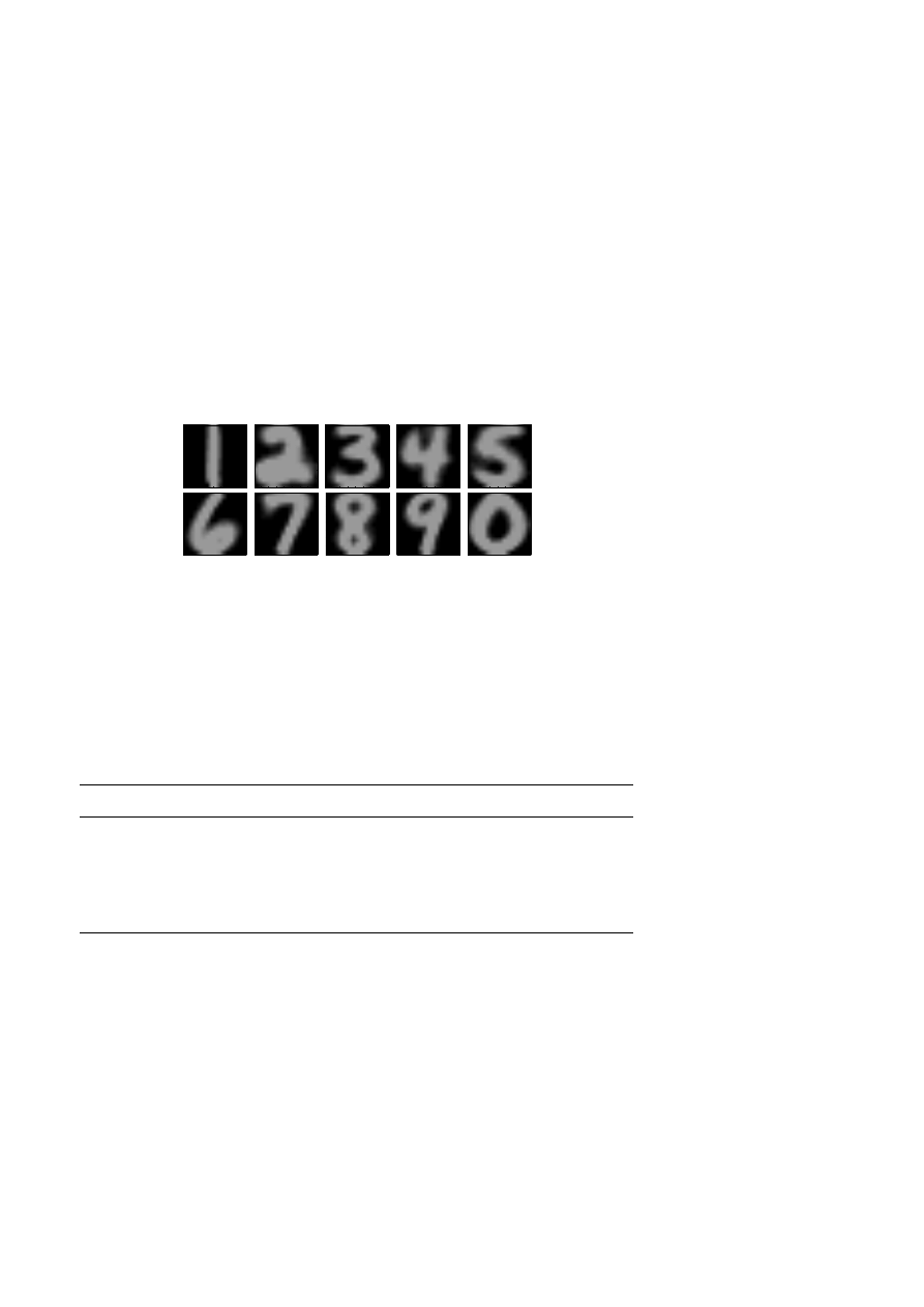
Figure 5.2. The means (centroids)
of all digits in the training set.

In Figure 5.2 we illustrate the means (centroids) of the digits in the train-

ing set. From this figure we get the impression that a majority of the digits
are well written (if there were many badly written digits this would demon-
strate itself as diffuse means). This means that the clusters are rather well
separated. Therefore it is likely that a simple algorithm that computes the
distance from each unknown digit to the means should work rather well.

A simple classification algorithm

Training. Given the training set, compute the mean (centroid) of all

digits of one kind.

Classification. For each digit in the test set, compute the distance to all

ten means, and classify as the closest.

360

L. Eld´

100

120

140

−

Figure 5.3. Singular values (top), and the first
three singular images (vectors) computed
using the 131 3s of the training set (bottom).

It turns out that for our test set the success rate of this algorithm is

around 75%, which is not good enough. The reason is that the algorithm
does not use any information about the variation of the digits of one kind.
This variation can be modelled using the SVD.

Let A ∈ R

×n

, with m = 256, be the matrix consisting of all the training

digits of one kind, the 3s, say. The columns of A span a linear subspace of
R

. However, this subspace cannot be expected to have a large dimension,

because if it had, then the subspaces of the different kinds of digits would
intersect.

The idea now is to ‘model’ the variation within the set of training digits

of one kind using an orthogonal basis of the subspace. An orthogonal basis
can be computed using the SVD, and A can be approximated by a sum of
rank-one matrices (3.9),

A =

Numerical linear algebra in data mining

361

for some value of k. Each column in A is an image of a digit 3, and therefore
the left singular vectors u

are an orthogonal basis in the ‘image space of 3s’.

We will refer to the left singular vectors as ‘singular images’. From the
matrix approximation properties of the SVD (Theorem 3.4) we know that
the first singular vector represents the ‘dominating’ direction of the data
matrix. Therefore, if we fold the vectors u

back to images, we expect

the first singular vector to look like a 3, and the following singular images
should represent the dominating variations of the training set around the
first singular image. In Figure 5.3 we illustrate the singular values and the
first three singular images for the training set 3s.

The SVD basis classification algorithm will be based on the following

assumptions.

(1) Each digit (in the training and test sets) is well characterized by a few

of the first singular images of its own kind. The more precise meaning
of ‘a few’ should be investigated by experiment.

(2) An expansion in terms of the first few singular images discriminates

well between the different classes of digits.

(3) If an unknown digit can be better approximated in one particular basis

of singular images, the basis of 3s say, than in the bases of the other
classes, then it is likely that the unknown digit is a 3.

Thus we should compute how well an unknown digit can be represented in

the ten different bases. This can be done by computing the residual vector
in least squares problems of the type

min

z −

where z represents an unknown digit, and u

the singular images. We can

write this problem in the form

min

z − U

where U

· · · u

. Since the columns of U

are orthogonal, the

solution of this problem is given by α = U

z, and the norm of the residual

vector of the least squares problems is

(I − U

(5.1)

It is interesting to see how the residual depends on the number of terms in

the basis. In Figure 5.4 we illustrate the approximation of a nicely written 3
in terms of the 3-basis with different numbers of basis images. In Figure 5.5
we show the approximation of a nice 3 in the 5-basis.

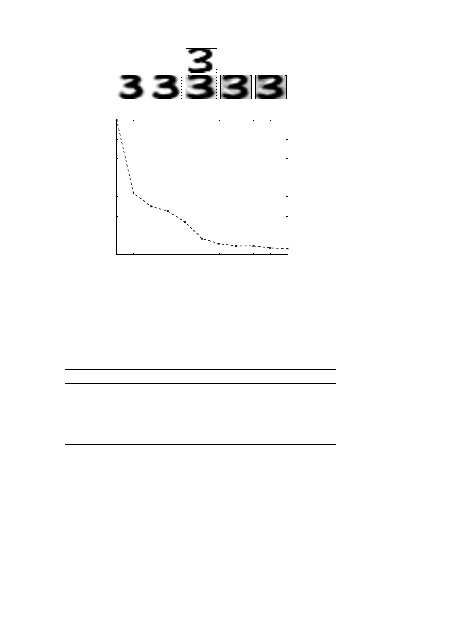
362

L. Eld´

0.3

0.4

0.5

0.6

0.7

0.8

0.9

relative residual

# basis vectors

Figure 5.4. Unknown digit (nice 3) and approximations
using 1, 3, 5, 7, and 9 terms in the 3-basis (top).
Relative residual (I − U

in least squares

problem (bottom).

From Figures 5.4 and 5.5 we see that the relative residual is considerably

smaller for the nice 3 in the 3-basis than in the 5-basis.

It is possible to devise several classification algorithm based on the model

of expanding in terms of SVD bases. Below we give a simple variant.

An SVD basis classification algorithm

Training. For the training set of known digits, compute the SVD of each

class of digits, and use k basis vectors for each class.

Classification. For a given test digit, compute its relative residual in all

ten bases. If one residual is significantly smaller than all the others,
classify as that. Otherwise give up.

The algorithm is closely related to the SIMCA method (Wold 1976,

Sj¨

ostr¨om and Wold 1980).

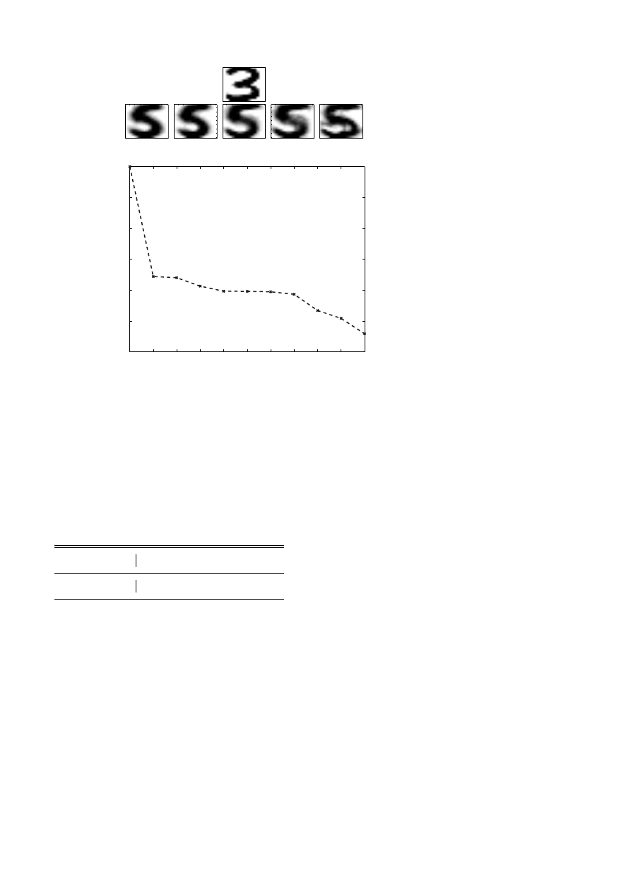
Numerical linear algebra in data mining

363

0.7

0.75

0.8

0.85

0.9

0.95

relative residual

# basis vectors

Figure 5.5. Unknown digit (nice 3) and approximations
using 1, 3, 5, 7, and 9 terms in the 5-basis (top).
Relative residual in least squares problem (bottom).

We next give some test results

for the US Postal Service data set, with

7291 training digits and 2007 test digits (Hastie et al. 2001). In Table 5.1
we give classification results as a function of the number of basis images for
each class.

Table 5.1. Correct classifications as a function of
the number of basis images (for each class).

# basis images

correct (%)

90.5

From Savas (2002).

364

L. Eld´

Even if there is a very significant improvement in performance compared

to the method where one only used the centroid images, the results are not
good enough, as the best algorithms reach about 97% correct classifications.

5.2. Tangent distance

Apparently it is the large variation in the way digits are written that makes
it difficult to classify correctly. In the preceding subsection we used SVD
bases to model the variation. An alternative model can be based on de-
scribing mathematically what are common and acceptable variations. We
illustrate a few such variations in Figure 5.6. In the first column of modified

Figure 5.6. A digit and acceptable transformations.

digits, the digits appear to be written

with a thinner and thicker pen, in

the second the digits have been stretched diagonal-wise, in the third they
have been compressed and elongated vertically, and in the fourth they have
been rotated. Such transformations constitute no difficulties for a human
reader and ideally they should be easy to deal with in automatic digit recog-
nition. A distance measure, tangent distance, that is invariant under small
transformations of this type is described in Simard et al. (1993, 2001).

For now we interpret 16 × 16 images as points in R

256

. Let p be a fixed

pattern in an image. We shall first consider the case of only one permit-
ted transformation, diagonal stretching, say. The transformation can be
thought of as moving the pattern along a curve in R

256

. Let the curve be

parametrized by a real parameter α so that the curve is given by s(p, α),
and in such a way that s(p, 0) = p. In general, such curves are nonlinear,
and can be approximated by the first two terms in the Taylor expansion,

s(p, α) = s(p, 0) +

dα

(p, 0) α + O(α

) ≈ p + t

α,

where t

dα

(p, 0) is a vector in R

256

. By varying α slightly around 0, we

Note that the modified digits have not been written manually but using the techniques
described later in this section. The presentation in this section is based on the papers
by Simard, LeCun and Denker (1993) and Simard, LeCun, Denker and Victorri (2001),
and the master’s thesis of Savas (2002).

Numerical linear algebra in data mining

365

make a small movement of the pattern along the tangent at the point p on
the curve. Assume that we have another pattern e that is approximated
similarly,

s(e, α) ≈ e + t

α.

Since we consider small movements along the curves as allowed, such small
movements should not influence the distance function. Therefore, ideally
we would like to define our measure of closeness between p and e as the
closest distance between the two curves.

In general we cannot compute the distance between the curves, but we

can use the first-order approximations. Thus we move the patterns indepen-
dently along their respective tangents, until we find the smallest distance.
If we measure this distance in the usual Euclidean norm, we shall solve the
least squares problem

min

,α

p + t

− e − t

= min

,α

(p − e) −

−t

Consider now the case when we are allowed to move the pattern p along

l different curves in R

256

, parametrized by α = (α

· · · α

)

. This is equiv-

alent to moving the pattern on an l-dimensional surface (manifold) in R

256

Assume that we have two patterns, p and e, each of which can move on its
surface of allowed transformations. Ideally we would like to find the clos-
est distance between the surfaces, but instead, since this is not possible to
compute, we now define a distance measure where we compute the distance
between the two tangent planes of the surface in the points p and e.

As before, the tangent plane is given by the first two terms in the Taylor

expansion of the function s(p, α):

s(p, α) = s(p, 0) +

dα

(p, 0) α

+ O(α

) ≈ p + T

α,

where T

is the matrix

dα

· · ·

dα

and the derivatives are all evaluated in the point (p, 0).

Thus the tangent distance between the points p and e is defined as the

smallest possible residual in the least squares problem

min

,α

p + T

− e − T

= min

,α

(p − e) −

−T

The least squares problem can be solved, e.g., using the QR decomposition
of A =

−T

. Note that we are in fact not interested in the solution

366

L. Eld´

itself but only in the norm of the residual. Write the least squares problem
in the form

min

b − Aα

b = p − e,

α =

With the QR decomposition

A = Q

= (Q

)

= Q

the norm of the residual is given by

min

b − Aα

= min

b − Rα

= min

b − Rα

+ Q

= Q

The case when the matrix A does not have full column rank is easily dealt
with using the SVD. The probability that the columns of the tangent matrix
are almost linearly dependent is high when the two patterns are close.

The most important property of this distance function is that it is invari-

ant under movements of the patterns on the tangent planes. For instance, if
we make a small translation in the x-direction of a pattern, then with this
measure the distance it has been moved is equal to zero.

Simard et al. (1993) and (2001) considered the following transformation:

horizontal and vertical translation, rotation, scaling, parallel and diagonal
hyperbolic transformation, and thickening. If we consider the image pattern
as a function of two variables, p = p(x, y), then the derivative of each
transformation can be expressed as a differentiation operator that is a linear
combination of the derivatives p

dp
dx

and p

dp
dy

. For instance, the

rotation derivative is

− xp

and the scaling derivative is

+ yp

The derivative of the diagonal hyperbolic transformation is

+ xp

and the ‘thickening’ derivative is

)

+ (p

)

has dimension 256 × 2l; since the number of transformations is usually less than 10,

the linear system is over-determined.

Numerical linear algebra in data mining

367

The algorithm is summarized as follows.

A tangent distance classification algorithm

Training. For each digit in the training set, compute its tangent ma-

trix T

Classification. For each test digit:

• Compute its tangent matrix.
• Compute the tangent distance to all training digits and classify it

as the one with shortest distance.

This algorithm is quite good in terms of classification performance (96.9%

correct classification for the US Postal Service data set (Savas 2002)), but
it is very expensive, since each test digit is compared to all the training
digits. In order to make it competitive it must be combined with some
other algorithm that reduces the number of tangent distance comparisons
to make.

We end this section by remarking that it is necessary to pre-process the

digits in different ways in order to enhance the classification: see LeCun
et al. (1998). For instance, performance is improved if the images are
smoothed (convolved with a Gaussian kernel): see Simard et al. (2001). In
Savas (2002) the derivatives p

and p

are computed numerically by finite

differences.

6. Eigenvalue methods in data mining

When an Internet search is made using a search engine, there is first a
traditional text processing part, where the aim is to find all the web pages
containing the words of the query. Because of the massive size of the Web,
the number of hits is likely to be much too large to be handled by the user.
Therefore, some measure of quality is needed to sort out the pages that are
likely to be most relevant to the particular query.

When one uses a web search engine, then typically the search phrase is

under-specified.

Example 6.1.

A Google search conducted on September 29, 2005, using

the search phrase university, gave as a result links to the following well-
known universities: Harvard , Stanford , Cambridge, Yale, Cornell , Oxford .
The total number of web pages relevant to the search phrase was more than
2 billion.

368

L. Eld´

Obviously Google uses an algorithm for ranking all the web pages that

agrees rather well with a common-sense quality measure. Loosely speaking,
Google assigns a high rank to a web page if it has inlinks from other pages
that have a high rank. We will see that this ‘self-referencing’ statement
can be formulated mathematically as an eigenvalue equation for a certain
matrix.

In the context of automatic text summarization, similar self-referencing

statements can be formulated mathematically as the defining equations of
a singular value problem. We treat this application briefly in Section 6.3.

6.1. PageRank

It is of course impossible to define a generally valid measure of relevance
that would be acceptable for a majority of users of a search engine. Google
uses the concept of PageRank as a quality measure of web pages. It is
based on the assumption that the number of links to and from a page give
information about the importance of a page. We will give a description of
PageRank based primarily on Page, Brin, Motwani and Winograd (1998).
Concerning Google, see Brin and Page (1998).

HHH

XXXX

XXXXX

XXXX

XXXXX

Figure 6.1. Inlinks and outlinks.

Let all web pages be ordered from 1 to n, and let i be a particular web

page. Then O

will denote the set of pages that i is linked to, the outlinks.

The number of outlinks is denoted by N

= |O

|. The set of inlinks, denoted

by I

, are the pages that have an outlink to i: see Figure 6.1.

In general, a page i can be considered as more important the more inlinks

it has. However, a ranking system based only on the number of inlinks
is easy to manipulate.

When you design a web page i that (e.g., for

commercial reasons) you would like to be seen by as many as possible, you
could simply create a large number of (information-less and unimportant)
pages that have outlinks to i. In order to discourage this, one may define

For an example of attempts to fool a search engine: see Totty and Mangalindan (2003).

Numerical linear algebra in data mining

369

the rank of i in such a way that if a highly ranked page j, has an outlink
to i, this should add to the importance of i in the following way: the rank
of page i is a weighted sum of the ranks of the pages that have outlinks to
i. The weighting is such that the rank of a page j is divided evenly among
its outlinks. The preliminary definition of PageRank is

∈I

i = 1, 2, . . . , n.

(6.1)

The definition (6.1) is recursive, so PageRank cannot be computed di-

rectly. The equation can be reformulated as an eigenvalue problem for a
matrix representing the graph of the Internet. Let Q be a square matrix of
dimension n, and let

1/N

if there is a link from j to i,

otherwise.

This definition means that row i has nonzero elements in those positions
that correspond to inlinks of i. Similarly, column j has nonzero elements
equal to N

in those positions that correspond to the outlinks of j, and,

provided that the page has outlinks, the sum of all the elements in column
j is equal to one. In the following symbolic picture of the matrix Q, nonzero
elements are denoted ∗:







∗
0

0 ∗ · · · ∗ ∗ · · ·

0
∗







← inlinks

↑

outlinks

Obviously, (6.1) can be written as

λr = Qr,

(6.2)

i.e., r is an eigenvector of Q with eigenvalue λ = 1. However, at this point
it is not clear that PageRank is well defined, as we do not know if there
exists an eigenvalue equal to 1.

It turns out that the theory of random walk and Markov chains gives

an intuitive explanation of the concepts involved. Assume that a surfer

370

L. Eld´

visiting a web page always chooses the next page among the outlinks with
equal probability. This random walk induces a Markov chain with transition
matrix Q

: see, e.g., Meyer (2000) and Langville and Meyer (2005a).

Markov chain is a random process for which the next state is determined
completely by the present state; the process has no memory. The eigenvector
r of the transition matrix with eigenvalue 1 corresponds to a stationary
probability distribution for the Markov chain: The element in position i, r

is the asymptotic probability that the random walker is at web page i.

The random surfer should never get stuck. In other words, there should

be no web pages without outlinks (such a page corresponds to a zero column
in Q). Therefore the model is modified so that zero columns are replaced
by a constant value in each position (equal probability to go to any other
page in the net). Define the vectors

if N

= 0,

otherwise,

for j = 1, . . . , n, and

e =







1
1







∈ R

Then the modified matrix is defined by

P = Q +

(6.3)

Now P is a proper column-stochastic matrix : it has nonnegative elements
(P ≥ 0), and

P = e

(6.4)

By analogy with (6.2), we would like to define the PageRank vector as a
unique eigenvector of P with eigenvalue 1,

P r = r.

However, uniqueness is still not guaranteed. To ensure this, the directed
graph corresponding to the matrix must be strongly connected : given any
two nodes (N

, N

), in the graph, there must exist a path leading from N

Note that we use a slightly different notation to that common in the theory of stochastic
processes.

Numerical linear algebra in data mining

371

to N

. In matrix terms, P must be irreducible.

Equivalently, there must

not exist any subgraph that has no outlinks.

The uniqueness of the eigenvalue is now guaranteed by the Perron–Fro-

benius theorem; we state it for the special case treated here.

Theorem 6.2.

Let A be an irreducible column-stochastic matrix. Then

the largest eigenvalue in magnitude is equal to 1. There is a unique cor-
responding eigenvector r satisfying r > 0, and r

= 1; this is the only

eigenvector that is nonnegative. If A > 0, then |λ

| < 1, i = 2, 3, . . . , n.

Proof.

Because A is column-stochastic we have e

A = e

, which means

that 1 is an eigenvalue of A. The rest of the statement can be proved using
Perron–Frobenius theory (Meyer 2000, Chapter 8).

Given the size of the Internet and reasonable assumptions about its struc-

ture, it is highly probable that the link graph is not strongly connected,
which means that the PageRank eigenvector of P is not well defined. To
ensure connectedness, i.e., to make it impossible for the random walker to
get trapped in a subgraph, one can add, artificially, a link from every web
page to all the other. In matrix terms, this can be made by taking a convex
combination of P and a rank-one matrix,

A = αP + (1 − α)

(6.5)

for some α satisfying 0 ≤ α ≤ 1. Obviously A is irreducible (since A > 0)
and column-stochastic:

A = αe

P + (1 − α)

= αe

+ (1 − α)e

= e

The random walk interpretation of the additional rank-one term is that each
time step a page is visited, the surfer will jump to any page in the whole
web with probability 1 − α (sometimes referred to as teleportation).

For the convergence of the numerical eigenvalue algorithm, it is essential

to know how the eigenvalues of P are changed by the rank one modifica-
tion (6.5).

Proposition 6.3.

Given that the eigenvalues of the column-stochastic

matrix P are {1, λ

, λ

. . . , λ

}, the eigenvalues of A = αP + (1 − α)

are {1, αλ

, αλ

, . . . , αλ

Several proofs of the proposition have been published (Haveliwala and

Kamvar 2003b, Langville and Meyer 2005a). An elementary and simple
variant (Eld´en 2004a) is given here.

A matrix P is reducible if there exist a permutation matrix Π such that ΠP Π

´, where both X and Z are square matrices.

372

L. Eld´

Proof.

Define ˆ

e to be e normalized to Euclidean length 1, and let U

∈

×(n−1)

be such that U =

e U

is orthogonal. Then, since ˆ

P = ˆ

P U =

e U

P ˆ

e U

w T

(6.6)

where w = U

P ˆ

e, and T = U

. Since we have made a similarity

transformation, the matrix T has the eigenvalues λ

, λ

, . . . , λ

. We further

have

v =

√

n e

√

Therefore,

AU = U

(αP + (1 − α)ve

= α

w T

+ (1 − α)

√

= α

w T

+ (1 − α)

√

n U

v 0

αT

The statement now follows immediately.

This means that even if P has a multiple eigenvalue equal to 1, the second-

largest eigenvalue in magnitude of A is always equal to α.

The vector e in (6.5) can be replaced by a nonnegative vector v with

= 1 that can be chosen in order to make the search biased towards

certain kinds of web pages. Therefore, it is referred to as a personalization
vector (Page et al. 1998, Haveliwala and Kamvar 2003a). The vector v can
also be used for avoiding manipulation by so-called link farms (Langville
and Meyer 2005a). Proposition 6.3 also holds in this case.

We want to solve the eigenvalue problem

Ar = r,

where r is normalized, r

= 1. Because of the sparsity and the dimension

of A it is not possible to use sparse eigenvalue algorithms that require the
storage of more than a very few vectors. The only viable method so far for
PageRank computations on the whole Web seems to be the power method.

It is well known (see, e.g., Golub and Van Loan (1996, Section 7.3)) that

the rate of convergence of the power method depends on the ratio of the
second-largest and the largest eigenvalue in magnitude. Here we have

|λ

(k)

− 1| = O(α

due to Proposition 6.3.

Numerical linear algebra in data mining

373

In view of the huge dimension of the Google matrix, it is nontrivial to

compute the matrix-vector product y = Az, where A = αP + (1 − α)

First, we see that if the vector z satisfies z

= e

z = 1, then

= e

y = e

Az = e

z = 1,

(6.7)

since A is column-stochastic (e

A = e

). Therefore normalization of the

vectors produced in the power iteration is unnecessary.

Then recall that P was constructed from the actual link matrix Q as

P = Q +

where the row vector d has an element 1 in all those positions that corre-
spond to web pages with no outlinks, see (6.3). This means that to represent
P as a sparse matrix, we insert a large number of full vectors in Q, each of
the same dimension as the total number of web pages. Consequently, one
cannot afford to represent P explicitly. Let us look at the multiplication
y = Az in some more detail:

y = α

Q +

z +

(1 − α)

e(e

z) = αQz + β

(6.8)

where

β = αd

z + (1 − α)e

However, we do not need to compute β from this equation. Instead we can
use (6.7) in combination with (6.8):

1 = e

(αQz) + βe

= e

(αQz) + β.

Thus, we have β = 1 − αQz

. An extra bonus is that we do not use the

vector d, i.e., we do not need to know which pages lack outlinks.

The following Matlab code implements the matrix vector multiplication.

yhat=alpha*Q*z;
beta=1-norm(yhat,1);
y=yhat+beta*v;
residual=norm(y-z,1);

Here v = (1/n) e, or a personalized teleportation vector: see p. 372.

From Proposition 6.3 we know that the second eigenvalue of the Google

matrix satisfies λ

= α. A typical value of α is 0.85. Approximately k = 57

iterations are needed to make the factor 0.85

equal to 10

−4

. This is reported

(Langville and Meyer 2005a) to be close the number of iterations used by
Google.

374

L. Eld´

In view of the fact that one PageRank calculation using the power method

can take several days, several enhancements of the iteration procedure have
been proposed. Kamvar, Haveliwala and Golub (2003a) describe an adap-
tive method that checks the convergence of the components of the PageRank
vector and avoids performing the power iteration for those components.
The block structure of the Web is used in Kamvar, Haveliwala, Manning
and Golub (2003b), and speed-ups of a factor 2 have been reported. An
acceleration method based on Aitken extrapolation is discussed in Kam-
var, Haveliwala, Manning and Golub (2003c). Aggregation methods are
discussed in several papers by Langville and Meyer and in Ipsen and Kirk-
land (2006).

If the PageRank is computed for a subset of the Internet, one particular

domain, say, then the matrix A may be of sufficiently small dimension to use
methods other than the power method: e.g., the Arnoldi method (Golub
and Greif 2004).

A variant of PageRank is proposed in Gy¨

ongyi, Garcia-Molina and Peder-

sen (2004). Further properties of the PageRank matrix are given in Serra-
Capizzano (2005).

6.2. HITS

Another method based on the link structure of the Web was introduced at
the same time as PageRank (Kleinberg 1999). It is called HITS (hyper-
text induced topic search), and is based on the concepts of authorities and
hubs. An authority is a web page with several inlinks and a hub has several
outlinks. The basic idea is: good hubs point to good authorities and good
authorities are pointed to by good hubs. Each web page is assigned both a
hub score y and an authority score x.

Let L be the adjacency matrix of the directed web graph. Then two

equations are given that mathematically define the relation between the
two scores, based on the basic idea:

x = L

y = Lx.

(6.9)

The algorithm for computing the scores is the power method, which con-
verges to the left and right singular vectors corresponding to the largest
singular value of L. In the implementation of HITS it is not the adja-
cency matrix of the whole web that is used, but of all the pages relevant to
the query.

There is now an extensive literature on PageRank, HITS and other rank-

ing methods. For overviews, see Langville and Meyer (2005b, 2005c) and
Berkin (2005). A combination of HITS and PageRank has been proposed
in Lempel and Moran (2001).

Obviously the ideas underlying PageRank and HITS are not restricted

Numerical linear algebra in data mining

375

to web applications, but can be applied to other network analyses. For
instance, a variant of the HITS method was recently used in a study of
Supreme Court precedent (Fowler and Jeon 2005). A generalization of HITS
is given in Blondel, Gajardo, Heymans, Senellart and Dooren (2004), which
also treats synonym extraction.

6.3. Text summarization

Because of the explosion in the amount of textual information available,
there is a need to develop automatic procedures for text summarization.
One typical situation is when a web search engine presents a small amount
of text from each document that matches a certain query. Another relevant
area is the summarization of news articles.

Automatic text summarization is an active research field with connec-

tions to several other research areas such as information retrieval, natural
language processing, and machine learning. Informally, the goal of text sum-
marization is to extract content from a text document, and present the most
important content to the user in a condensed form and in a manner sensi-
tive to the user’s or application’s need (Mani 2001). In this section we will
have a considerably less ambitious goal: we present a method (Zha 2002),
related to HITS, for automatically extracting key words and key sentences
from a text. There are connections to the vector space model in information
retrieval, and to the concept of PageRank.

Consider a text from which we want to extract key words and key sen-

tences. As one of the preprocessing steps, one should perform stemming
and eliminate stop words. Similarly, if the text carries special symbols,
e.g., mathematics, or mark-up language tags (HTML, L

TEX), it may be

necessary to remove those. Since we want to compare word frequencies in
different sentences, we must consider each sentence as a separate document
(in the terminology of information retrieval). After the preprocessing has
been done, we parse the text, using the same type of parser as in infor-
mation retrieval. This way a term-document matrix is prepared, which in
this section we will refer to as a term-sentence matrix. Thus we have a
matrix A ∈ R

×n

, where m denotes the number of different terms, and n

the number of sentences. The element a

is defined as the frequency

term i in document j.

The basis of the procedure in Zha (2002) is the simultaneous, but separate

ranking of the terms and the sentences. Thus, term i is given a nonnegative
saliency score, denoted u

. The higher the saliency score, the more impor-

tant the term. The saliency score of sentence j is denoted by v

Naturally, a term and document weighting scheme (see Berry and Browne (2005, Sec-
tion 3.2.1)) should be used.

376

L. Eld´

The assignment of saliency scores is made based on the mutual reinforce-

ment principle (Zha 2002):

A term should have a high saliency score if it appears in many sentences with high
saliency scores. A sentence should have a high saliency score if it contains many
words with high saliency scores.

More precisely, we assert that the saliency score of term i is proportional to
the sum of the scores of the sentences where it appears; in addition, each
term is weighted by the corresponding matrix element,

∝

i = 1, 2, . . . , m.

Similarly, the saliency score of sentence j is defined to be proportional to
the scores of its words, weighted by the corresponding a

∝

j = 1, 2, . . . , n.

Collecting the saliency scores in two vectors, u ∈ R

, and v ∈ R

, these

two equations can be written as

u = Av,

(6.10)

v = A

(6.11)

where σ

and σ

are proportionality constants. In fact, the constants must

be equal: inserting one equation into the other, we get

u =

v =

Av,

which shows that u and v are singular vectors corresponding to the same sin-
gular value. If we choose the largest singular value, then we are guaranteed
that the components of u and v are nonnegative.

Example 6.4.

We created a term-sentence matrix using (a slightly earlier

version of) the text in Section 4. Since the text is written using L

TEX, we

first had to remove all L

TEX typesetting commands. This was done using

a lexical scanner called detex.

Then the text was stemmed and stop

words were removed. A term-sentence matrix A was constructed using a
text parser: there turned out to be 435 terms in 218 sentences. The first
singular vectors were computed in Matlab.

http://www.cs.purdue.edu/homes/trinkle/detex/

Numerical linear algebra in data mining

377

By determining the ten largest components of u

, and using the dictionary

produced by the text parser, we found that the following ten words are the
most important in the section.

document, term, matrix , approximation (approximate), query, vector , space,
number , basis, cluster .

The three most important sentences are, in order, as follows.

(1) Latent semantic indexing (LSI) ‘is based on the assumption that there

is some underlying latent semantic structure in the data . . . that is cor-
rupted by the wide variety of words used . . . ’ (quoted from Park, Jeon
and Rosen (2001)) and that this semantic structure can be enhanced by
projecting the data (the term-document matrix and the queries) onto
a lower-dimensional space using the singular value decomposition.

(2) In view of the large approximation error in the truncated SVD approx-

imation of the term-document matrix, one may question whether the
‘optimal’ singular vectors constitute the best basis for representing the
term-document matrix.

(3) For example, one can define the elements in A by

= f

log(n/n

where f

is the term frequency, the number of times term i appears

in document j, and n

is the number of documents that contain term

i (inverse document frequency).

It is apparent that this method prefers long sentences. On the other hand,
these sentences are undeniably key sentences for the text.

7. New directions

Multidimensional arrays (tensors) have been used for data analysis in psy-
chometrics and chemometrics since the 1960s; for overviews see, e.g., Kroo-
nenberg (1992), Smilde, Bro and Geladi (2004) and the ‘Three-Mode Com-
pany’ web page.

In fact, ‘three-mode analysis’ appears to be a standard

tool in those areas. Only in recent years has there been an increased interest
among the numerical linear algebra community in tensor computations, es-
pecially for applications in signal processing and data mining. A particular
generalization of the SVD, the higher order SVD (HOSVD), was studied in
Lathauwer, Moor and Vandewalle (2000a).

This is a tensor decomposition

http://three-mode.leidenuniv.nl/

However, related concepts had already been considered in Tucker (1964) and (1966),
and are referred to as the Tucker model in psychometrics.

378

L. Eld´

in terms of orthogonal matrices, which ‘orders’ the tensor in a way similar
to that in which the singular values of the SVD are ordered, but which
does not satisfy an Eckart–Young optimality property (Theorem 3.4); see
Lathauwer, Moor and Vandewalle (2000b). Owing to the ordering property,
this decomposition can be used for compression and dimensionality reduc-
tion, and it has been successfully applied to face recognition (Vasilescu and
Terzopoulos 2002a, 2002b, 2003).

The SVD expansion (3.9) of a matrix, as a sum of rank-one matrices,

has been generalized to tensors (Harshman 1970, Carroll and Chang 1970),
and is called the PARAFAC/CANDECOMP model. For overviews, see Bro
(1997) and Smilde et al. (2004). This does not give an exact decomposition
of the tensor, and its theoretical properties are much more involved (e.g.,
degeneracies occur – see Kruskal (1976, 1977), Bro (1997) and Sidiropoulos
and Bro (2000)). A recent application of PARAFAC to network analysis is
presented in Kolda, Bader and Kenny (2005a), where the hub and authority
scores of the HITS method are complemented with topic scores for the
anchor text of the web pages.

Recently several papers have appeared where standard techniques in data

analysis and machine learning are generalized to tensors: see, e.g., Yan, Xu,
Yang, Zhang, Tang and Zhang (2005) and Cai, He and Han (2005).

It is not uncommon in the data mining/machine learning literature for

data compression and rank reduction problems to be presented as matrix
problems, while they can in fact be considered as tensor approximation
problems: for examples see Tenenbaum and Freeman (2000) and Ye (2005).

Novel data mining applications, especially in link structure analysis, are

presented and suggested in Kolda, Brown, Corones, Critchlow, Eliassi-
Rad, Getoor, Hendrickson, Kumar, Lambert, Matarazzo, McCurley, Merrill,
Samatova, Speck, Srikant, Thomas, Wertheimer and Wong (2005b).

REFERENCES

R. Baeza-Yates and B. Ribeiro-Neto (1999), Modern Information Retrieval, ACM

Press, Addison-Wesley, New York.

B. Bergeron (2002), Bioinformatics Computing, Prentice-Hall.
P. Berkin (2005), ‘A survey on PageRank computing’, Internet Mathematics 2,

73–120.

M. Berry, ed. (2001), Computational Information Retrieval, SIAM, Philadelphia,

PA.

M. Berry and M. Browne (2005), Understanding Search Engines: Mathematical

Modeling and Text Retrieval, 2nd edn, SIAM, Philadelphia, PA.

M. Berry and G. Linoff (2000), Mastering Data Mining: The Art and Science of

Customer Relationship Management, Wiley, New York.

M. Berry, Z. Drmac and E. Jessup (1999), ‘Matrices, vector spaces and information

retrieval’, SIAM Review 41, 335–362.

Numerical linear algebra in data mining

379

M. Berry, S. Dumais and G. O’Brien (1995), ‘Using linear algebra for intelligent

information retrieval’, SIAM Review 37, 573–595.

A. Bj¨

orck (1996), Numerical Methods for Least Squares Problems, SIAM, Philadel-
phia, PA.

K. Blom and A. Ruhe (2005), ‘A Krylov subspace method for information retrieval’,

SIAM J. Matrix Anal. Appl. 26, 566–582.

V. D. Blondel, A. Gajardo, M. Heymans, P. Senellart and P. V. Dooren (2004),

‘A measure of similarity between graph vertices: Applications to synonym
extraction and web searching’, SIAM Review 46, 647–666.

S. Brin and L. Page (1998), ‘The anatomy of a large-scale hypertextual web search

engine’, Computer Networks and ISDN Systems 30, 107–117.

R. Bro (1997), ‘PARAFAC: Tutorial and applications’, Chemometrics and Intelli-

gent Laboratory Systems 38, 149–171.

M. Burl, L. Asker, P. Smyth, U. Fayyad, P. Perona, L. Crumpler and J. Aubele

(1998), ‘Learning to recognize volcanoes on Venus’, Machine Learning
30, 165–195.

D. Cai, X. He and J. Han (2005), Subspace learning based on tensor analysis.

Technical Report UIUCDCS-R-2005-2572, UILU-ENG-2005-1767, Computer
Science Department, University of Illinois, Urbana-Champaign.

J. D. Carroll and J. J. Chang (1970), ‘Analysis of individual differences in multi-

dimensional scaling via an N-way generalization of “Eckart–Young” decom-
position’, Psychometrika 35, 283–319.

N. Christianini and J. Shawe-Taylor (2000), An Introduction to Support Vector

Machines, Cambridge University Press.

M. Chu, R. Funderlic and G. Golub (1995), ‘A rank-one reduction formula and its

applications to matrix factorization’, SIAM Review 37, 512–530.

K. Cios, W. Pedrycz and R. Swiniarski (1998), Data Mining: Methods for Knowl-

edge Discovery, Kluwer, Boston.

B. De Moor and P. Van Dooren (1992), ‘Generalizations of the singular value and

QR decompositions’, SIAM J. Matrix Anal. Appl. 13, 993–1014.

S. Deerwester, S. Dumais, G. Furnas, T. Landauer and R. Harsman (1990), ‘In-

dexing by latent semantic analysis’, J. Amer. Soc. Information Science 41,
391–407.

I. Dhillon (2001), Co-clustering documents and words using bipartite spectral graph

partitioning, in Proc. 7th ACM–SIGKDD Conference, pp. 269–274.

I. Dhillon and D. Modha (2001), ‘Concept decompositions for large sparse text

data using clustering’, Machine Learning 42, 143–175.

I. Dhillon, J. Fan and Y. Guan (2001), Efficient clustering of very large docu-

ment collections, in Data Mining For Scientific and Engineering Applications
(V. Grossman, C. Kamath and R. Namburu, eds), Kluwer.

I. Dhillon, Y. Guan and B. Kulis (2005), A unified view of kernel k-means, spec-

tral clustering and graph partitioning. Technical Report UTCS TR-04-25,
University of Texas at Austin, Department of Computer Sciences.

D. Di Ruscio (2000), ‘A weighted view on the partial least-squares algorithm’,

Automatica 36, 831–850.

R. Duda, P. Hart and D. Storck (2001), Pattern Classification, 2nd edn, Wiley-

Interscience.

380

L. Eld´

G. Eckart and G. Young (1936), ‘The approximation of one matrix by another of

lower rank’, Psychometrika 1, 211–218.

J. Einbeck, G. Tutz and L. Evers (2005), ‘Local principal curves’, Statistics and

Computing 15, 301–313.

L. Eld´en (2004a), The eigenvalues of the Google matrix. Technical Report LiTH-

MAT-R–04-01, Department of Mathematics, Link¨

oping University.

L. Eld´en (2004b), ‘Partial least squares vs. Lanczos bidiagonalization I: Analysis

of a projection method for multiple regression’, Comput. Statist. Data Anal.
46, 11–31.

U. Fayyad, G. Piatetsky-Shapiro, P. Smyth and R. Uthurusamy, eds (1996), Ad-

vances in Knowledge Discovery and Data Mining, AAAI Press/The MIT
Press, Menlo Park, CA.

J. Fowler and S. Jeon (2005), The authority of supreme court precedent: A network

analysis. Technical report, Department of Political Science, UC Davis.

I. Frank and J. Friedman (1993), ‘A statistical view of some chemometrics regres-

sion tools’, Technometrics 35, 109–135.

J. Giles, L. Wo and M. Berry (2003), GTP (General Text Parser) software for text

mining, in Statistical Data Mining and Knowledge Discovery (H. Bozdogan,
ed.), CRC Press, Boca Raton, pp. 455–471.

N. Goharian, A. Jain and Q. Sun (2003), ‘Comparative analysis of sparse matrix al-

gorithms for information retrieval’, J. Systemics, Cybernetics and Informatics
1(1).

G. Golub and C. Greif (2004), Arnoldi-type algorithms for computing stationary

distribution vectors, with application to PageRank. Technical Report SCCM-
04-15, Department of Computer Science, Stanford University.

G. H. Golub and W. Kahan (1965), ‘Calculating the singular values and pseudo-

inverse of a matrix’, SIAM J. Numer. Anal. Ser. B 2, 205–224.

G. H. Golub and C. F. Van Loan (1996), Matrix Computations, 3rd edn, Johns

Hopkins Press, Baltimore, MD.

G. Golub, K. Sølna and P. Van Dooren (2000), ‘Computing the SVD of a general

matrix product/quotient’, SIAM J. Matrix Anal. Appl. 22, 1–19.

D. Grossman and O. Frieder (1998), Information Retrieval: Algorithms and Heuris-

tics, Kluwer.

L. Guttman (1957), ‘A necessary and sufficient formula for matrix factoring’, Psy-

chometrika 22, 79–81.

Z. Gy¨

ongyi, H. Garcia-Molina and J. Pedersen (2004), Combating web spam with

TrustRank, in Proc. 30th International Conference on Very Large Databases,
Morgan Kaufmann, pp. 576–587.

J. Han and M. Kamber (2001), Data Mining: Concepts and Techniques, Morgan

Kaufmann, San Francisco.

D. Hand, H. Mannila and P. Smyth (2001), Principles of Data Mining, MIT Press,

Cambridge, MA.

R. A. Harshman (1970), ‘Foundations of the PARAFAC procedure: Models and

conditions for an “explanatory” multi-modal factor analysis’, UCLA Working
Papers in Phonetics 16, 1–84.

T. Hastie (1984), Principal curves and surfaces. Technical report, Stanford Uni-

versity.

Numerical linear algebra in data mining

381

T. Hastie, R. Tibshirani and J. Friedman (2001), The Elements of Statistical Learn-

ing: Data mining, Inference and Prediction, Springer, New York.

T. Haveliwala and S. Kamvar (2003a), An analytical comparison of approaches

to personalizing PageRank. Technical report, Computer Science Department,
Stanford University.

T. Haveliwala and S. Kamvar (2003b), The second eigenvalue of the Google matrix.

Technical report, Computer Science Department, Stanford University.

M. Hegland (2001), ‘Data mining techniques’, in Acta Numerica, Vol. 10, Cam-

bridge University Press, pp. 313–355.

I. Helland (1988), ‘On the structure of partial least squares regression’, Commun.

Statist. Simulation 17, 581–607.

P. Howland and H. Park (2004), ‘Generalizing discriminant analysis using the gen-

eralized singular value decomposition’, IEEE Trans. Pattern Anal. Machine
Intelligence 26, 995– 1006.

P. Howland, M. Jeon and H. Park (2003), ‘Structure preserving dimension reduc-

tion based on the generalized singular value decomposition’, SIAM J. Matrix
Anal. Appl. 25, 165–179.

L. Hubert, J. Meulman and W. Heiser (2000), ‘Two purposes for matrix factoriza-

tion: A historical appraisal’, SIAM Review 42, 68–82.

I. C. Ipsen and S. Kirkland (2006), ‘Convergence analysis of a Pagerank updating

algorithm by Langville and Meyer’, SIAM J. Matrix Anal. Appl. 27, 952–967.

E. Jessup and J. Martin (2001), Taking a new look at the latent semantic analysis

approach to information retrieval, in Computational Information Retrieval
(M. Berry, ed.), SIAM, Philadelphia, PA, pp. 121–144.

I. Joliffe (1986), Principal Component Analysis, Springer, New York.
S. Kamvar, T. Haveliwala and G. Golub (2003a), ‘Adaptive methods for the com-

putation of PageRank’, Linear Algebra Appl. 386, 51–65.

S. Kamvar, T. Haveliwala, C. Manning and G. Golub (2003b), Exploiting the block

structure of the Web for computing PageRank. Technical report, Computer
Science Department, Stanford University.

S. Kamvar, T. Haveliwala, C. Manning and G. Golub (2003c), Extrapolation

methods for accelerating PageRank computations, in Proc. 12th International
World Wide Web Conference, Budapest, May 2003, pp. 261–270.

J. M. Kleinberg (1999), ‘Authoritative sources in a hyperlinked environment’,

J. Assoc. Comput. Mach. 46, 604–632.

T. Kolda, B. Bader and J. Kenny (2005a), Higher-order web link analysis us-

ing multilinear algebra, in Proc. 5th IEEE International Conference on Data
Mining, ICDM05, IEEE Computer Society Press.

T. Kolda, D. Brown, J. Corones, T. Critchlow, T. Eliassi-Rad, L. Getoor, B. Hen-

drickson, V. Kumar, D. Lambert, C. Matarazzo, K. McCurley, M. Merrill,
N. Samatova, D. Speck, R. Srikant, J. Thomas, M. Wertheimer and P. C.
Wong (2005b), Data sciences technology for homeland security information
management and knowledge discovery. Technical Report SAND2004-6648,
Sandia National Laboratories.

R. Korfhage (1997), Information Storage and Retrieval, Wiley, New York.
P. M. Kroonenberg (1992), ‘Three-mode component models: A survey of the liter-

ature’, Statistica Applicata 4, 619–633.

382

L. Eld´

J. B. Kruskal (1976), ‘More factors than subjects, tests and treatments: An in-

determinacy theorem for canonical decomposition and individual differences
scaling’, Psychometrika 41, 281–293.

J. B. Kruskal (1977), ‘Three-way arrays: Rank and uniqueness of trilinear decompo-

sitions, with application to arithmetic complexity and statistics (Corrections,
17-1-1984; available from author)’, Linear Algebra Appl. 18, 95–138.

A. Langville and C. Meyer (2005a), ‘Deeper inside PageRank’, Internet Mathemat-

ics 1, 335–380.

A. N. Langville and C. D. Meyer (2005b), ‘A survey of eigenvector methods for

web information retrieval’, SIAM Review 47, 135–161.

A. N. Langville and C. D. Meyer (2005c), Understanding Web Search Engine Rank-

ings: Google’s PageRank, Teoma’s HITS, and Other Ranking Algorithms,
Princeton University Press.

L. D. Lathauwer, B. D. Moor and J. Vandewalle (2000a), ‘A multilinear singular

value decomposition’, SIAM J. Matrix Anal. Appl. 21, 1253–1278.

L. D. Lathauwer, B. D. Moor and J. Vandewalle (2000b), ‘On the best rank-1

and rank-(R

, R

, . . . , R

) approximation of higher-order tensor’, SIAM J.

Matrix Anal. Appl. 21, 1324–1342.

Y. LeCun, L. Bottou, Y. Bengio and P. Haffner (1998), ‘Gradient-based learning

applied to document recognition’, Proc. IEEE 86, 2278–2324.

R. Lempel and S. Moran (2001), ‘Salsa: the stochastic approach for link-structure

analysis’, ACM Trans. Inf. Syst. 19, 131–160.

I. Mani (2001), Automatic Summarization, John Benjamins.
W. Massy (1965), ‘Principal components regression in exploratory statistical re-

search’, J. Amer. Statist. Assoc. 60, 234–246.

J. Mena (1999), Data Mining Your Website, Digital Press, Boston.
C. Meyer (2000), Matrix Analysis and Applied Linear Algebra, SIAM, Philadelphia.
L. Mirsky (1960), ‘Symmetric gauge functions and unitarily invariant norms’,

Quart. J. Math. Oxford 11, 50–59.

C. Moler (2002), ‘The world’s largest matrix computation’, Matlab News and Notes,

October 2002, pp. 12–13.

L. Page, S. Brin, R. Motwani and T. Winograd (1998), ‘The PageRank citation

ranking: Bringing order to the Web’, Stanford Digital Library Working Pa-
pers.

C. Paige and M. Saunders (1981), ‘Towards a generalized singular value decompo-

sition’, SIAM J. Numer. Anal. 18, 398–405.

C. Paige and M. Saunders (1982), ‘LSQR: An algorithm for sparse linear equations

and sparse least squares’, ACM Trans. Math. Software 8, 43–71.

H. Park and L. Eld´en (2005), Matrix rank reduction for data analysis and fea-

ture extraction, in Handbook of Parallel Computing and Statistics (E. Konto-
ghiorghes, ed.), CRC Press, Boca Raton.

H. Park, M. Jeon and J. B. Rosen (2001), Lower dimensional representation of text

data in vector space based information retrieval, in Computational Informa-
tion Retrieval (M. Berry, ed.), SIAM, Philadelphia, PA, pp. 3–23.

H. Park, M. Jeon and J. B. Rosen (2003), ‘Lower dimensional representation of

text data based on centroids and least squares’, BIT 43, 427–448.

Numerical linear algebra in data mining

383

A. Phatak and F. de Hoog (2002), ‘Exploiting the connection between PLS, Lanczos

methods and conjugate gradients: Alternative proofs of some properties of
PLS’, J. Chemometrics 16, 361–367.

Y. Saad (2003), Iterative Methods for Sparse Linear Systems, 2nd edn, SIAM.
G. Salton, C. Yang and A. Wong (1975), ‘A vector-space model for automatic

indexing’, Comm. Assoc. Comput. Mach. 18, 613–620.

B. Savas (2002), Analyses and test of handwritten digit algorithms. Master’s thesis,

Mathematics Department, Link¨

oping University.

S. Serra-Capizzano (2005), ‘Jordan canonical form of the Google matrix: A poten-

tial contribution to the Pagerank computation’, SIAM J. Matrix Anal. Appl.
27, 305–312.

N. D. Sidiropoulos and R. Bro (2000), ‘On the uniqueness of multilinear decompo-

sition of N -way arrays’, J. Chemometrics 14, 229–239.

P. Simard, Y. LeCun and J. Denker (1993), Efficient pattern recognition using a

new transformation distance, in Advances in Neural Information Processing
Systems 5 (J. Cowan, S. Hanson and C. Giles, eds), Morgan Kaufmann,
pp. 50–58.

P. Simard, Y. LeCun, J. Denker and B. Victorri (2001), ‘Transformation invariance

in pattern recognition: Tangent distance and tangent propagation’, Internat.
J. Imaging System Techn. 11, 181–194.

H. D. Simon, A. Sohn and R. Biswas (1998), ‘Harp: A dynamic spectral parti-

tioner.’, J. Parallel Distrib. Comput. 50, 83–103.

M. Sj¨

ostr¨

om and S. Wold (1980), SIMCA: A pattern recognition method based on

principal components models, in Pattern Recognition in Practice (E. S. Gel-
sema and L. N. Kanal, eds), North-Holland, pp. 351–359.

A. Smilde, R. Bro and P. Geladi (2004), Multi-Way Analysis: Applications in the

Chemical Sciences, Wiley.

J. Tenenbaum and W. Freeman (2000), ‘Separating style and content with bilinear

models’, Neural Computation 12, 1247–1283.

M. Totty and M. Mangalindan (2003), ‘As Google becomes Web’s gatekeeper, sites

fight to get in’, Wall Street Journal CCXLI.

L. Tucker (1964), The extension of factor analysis to three-dimensional matrices, in

Contributions to Mathematical Psychology (H. Gulliksen and N. Frederiksen,
eds), Holt, Rinehart and Winston, New York, pp. 109–127.

L. Tucker (1966), ‘Some mathematical notes on three-mode factor analysis’, Psy-

chometrika 31, 279–311.

C. Van Loan (1976), ‘Generalizing the singular value decomposition’, SIAM J.

Numer. Anal. 13, 76–83.

M. Vasilescu and D. Terzopoulos (2002a), Multilinear analysis of image ensem-

bles: Tensorfaces, in Proc. 7th European Conference on Computer Vision
(ECCV’02), Vol. 2350 of Lecture Notes in Computer Science, Springer,
Copenhagen, Denmark, pp. 447–460.

M. Vasilescu and D. Terzopoulos (2002b), Multilinear image analysis for facial

recognition, in International Conference on Pattern Recognition, Quebec City,
Canada (ICPR ’02), IEEE Computer Society, pp. 511–514.

384

L. Eld´

M. Vasilescu and D. Terzopoulos (2003), Multilinear subspace analysis of image

ensembles, in IEEE Conference on Computer Vision and Pattern Recognition,
Madison WI (CVPR’03), pp. 93–99.

J. Wedderburn (1934), Lectures on Matrices, Colloquium Publications, AMS, New

York.

I. Witten and E. Frank (2000), Data Mining: Practical Machine Learning Tools and

Techniques with Java Implementations, Morgan Kaufmann, San Francisco.

H. Wold (1975), Soft modeling by latent variables: The nonlinear iterative partial

least squares approach, in Perspectives in Probability and Statistics: Papers
in Honour of M. S. Bartlett (J. Gani, ed.), Academic Press, London.

S. Wold (1976), ‘Pattern recognition by means of disjoint principal components

models’, Pattern Recognition 8, 127–139.

S. Wold, A. Ruhe, H. Wold and W. Dunn (1984), ‘The collinearity problem in

linear regression: The partial least squares (PLS) approach to generalized
inverses’, SIAM J. Sci. Statist. Comput. 5, 735–743.

S. Wold, M. Sj¨

ostr¨

om and L. Eriksson (2001), ‘PLS-regression: A basic tool of

chemometrics’, Chemometrics and Intell. Lab. Systems 58, 109–130.

S. Yan, D. Xu, Q. Yang, L. Zhang, X. Tang and H. Zhang (2005), Discriminant

analysis with tensor representation, in Proc. 2005 IEEE Computer Society
Conference on Computer Vision and Pattern Recognition (CVPR’05).

J. Ye (2005), ‘Generalized low rank approximations of matrices’, Machine Learning

61, 167–191.

D. Zeimpekis and E. Gallopoulos (2005), Design of a MATLAB toolbox for term-

document matrix generation, in Proc. Workshop on Clustering High Dimen-
sional Data and its Applications (I. Dhillon, J. Kogan and J. Ghosh, eds),
Newport Beach, CA, pp. 38–48.

H. Zha (2002), Generic summarization and keyphrase extraction using mutual re-

inforcement principle and sentence clustering, in Proc. 25th Annual Interna-
tional ACM–SIGIR Conference on Research and Development in Information
Retrieval, Tampere, Finland, pp. 113–120.

H. Zha, C. Ding, M. Gu, X. He and H. Simon (2002), Spectral relaxation for

k-means clustering, in Advances in Neural Information Processing Systems
(T. Dietterich, S. Becker and Z. Ghahramani, eds), MIT Press, pp. 1057–
1064.

Wyszukiwarka

Podobne podstrony:
tutorial4 Numerical Linear Algebra
IEEE Finding Patterns in Three Dimensional Graphs Algorithms and Applications to Scientific Data Mi
tutorial3 Using MATLAB in Linear Algebra
Dodatkowe Wytyczne projektu, Data mining - Grzenda
Data mining w rekomendacji
Metodologia w VIII, WYBRANE METODY ANALIZY WIELOZMIENNOWEJ - PODSTAWOWE ZAŁOŻENIA ANALIZY CZYNNIKOWE
(Sas Code) Data Mining Cookbook (Wiley)
Linear Algebra, Infinite Dimensions, and Maple, Preface
10 Data Storage in Data Blocksid 10809 ppt
Scoring kredytowy a modele data mining
(ebook pdf) Mathematics Abstract And Linear Algebra PJFCT5UIYCCSHOYDU7JHPAKULMLYEBKKOCB7OWA
Connell Elements of abstract and linear algebra(146s)
data mining zadania
Detecting Internet Worms Using Data Mining Techniques

więcej podobnych podstron