Accelerating numerical solution of Stochastic

Differential Equations with CUDA

M. Januszewski, M. Kostur

a

a

Institute of Physics, University of Silesia, 40-007 Katowice, Poland

Abstract

Numerical integration of stochastic differential equations is commonly used in

many branches of science. In this paper we present how to accelerate this kind of

numerical calculations with popular NVIDIA Graphics Processing Units using

the CUDA programming environment. We address general aspects of numerical

programming on stream processors and illustrate them by two examples: the

noisy phase dynamics in a Josephson junction and the noisy Kuramoto model.

In presented cases the measured speedup can be as high as 675× compared to a

typical CPU, which corresponds to several billion integration steps per second.

This means that calculations which took weeks can now be completed in less

than one hour. This brings stochastic simulation to a completely new level,

opening for research a whole new range of problems which can now be solved

interactively.

Key words:

Josephson junction, Kuramoto, graphics processing unit,

advanced computer architecture, numerical integration, diffusion, stochastic

differential equation, CUDA, Tesla, NVIDIA

1. Introduction

The numerical integration of stochastic differential equations (SDEs) is a

valuable tool for analysis of a vast diversity of problems in physics, ranging from

equilibrium transport in molecular motors [1], phase dynamics in Josephson

junctions [2, 3], stochastic resonance [4] to dissipative particle dynamics [5] to

finance [6]. Stochastic simulation, as it is referred to as, is specially interesting

when the dimensionality of the problem is larger than three, and in that case

it is often the only effective numerical method. A prominent example of this is

the stochastic variation of molecular dynamics: Brownian dynamics.

Direct stochastic simulations require a significant computational effort, and

therefore merely a decade ago have been used mostly as validation tools. The

precise numerical results in theory of low-dimensional stochastic problems were

coming from solutions of the corresponding Fokker-Planck equations. Many

different sophisticated, but often complicated, tools have been applied: spectral

methods [7, 8, 9], finite element methods [10] and numerical path integrals

[11, 12].

Preprint submitted to Elsevier

August 12, 2009

arXiv:0903.3852v2 [physics.comp-ph] 12 Aug 2009

Stochastic simulation gained acceptance due to its straightforward imple-

mentation and generic robustness with respect to different sorts of problems.

The continuous increase of the efficiency of available computer hardware has

been acting in favour of stochastic simulation, making it increasingly more pop-

ular. The recent evolution of computer architectures towards multiprocessor

and multicore platforms also resulted in improved performance of stochastic

simulation. Let us note that in the case of a low-dimensional system, stochastic

simulation often uses ensemble averaging to obtain the values of observables,

which in turn is an example of a so-called ,,embarrassingly parallel problem”

and it can, though with embarrassment, directly benefit from a parallel archi-

tecture. In other cases, mostly where a large number of interacting subsystems

are investigated, the implementation of the problem on a parallel architecture

is less trivial, but still possible.

The recent emergence of techniques collectively known as general-purpose

computing on graphics processing units (GPUs) has caused a breakthrough in

computational science. The current state of the art GPUs are now capable of

performing computations at a rate of about 1 TFLOPS per single silicon chip.

It must be stressed that 1 TFLOPS is a performance level which only in 1996

was achievable exclusively by huge and expensive supercomputers such as the

ASCI Red Supercomputer (which had a peak performance of 1.8 TFLOPS [13])

The numerical simulations of SDEs can easily benefit from the parallel GPU

architecture. This however requires careful redesign of the employed algorithms

and in general cannot be done automatically. In this paper we present a practical

introduction to solving SDEs on NVIDIA GPUs using Compute Unified Device

Architecture (CUDA) [14] based on two examples: the model of phase diffusion

in a Josephson junction and the Kuramoto model of coupled phase oscillators.

The paper is organized as follows: first, we briefly introduce the features and

capabilities of the NVIDIA CUDA environment and describe the two physical

models, then we present the implementation of stochastic algorithms and com-

pare their efficiency with a corresponding pure-CPU implementation executed

on an Intel Core2 Duo E6750 processor. We also provide the source code [15] of

three small example programs: PROG1, PROG2, and PROG3, which demon-

strate the techniques described in the paper. They can easily be extended to a

broad range of problems involving stochastic differential equations.

2. The CUDA environment

CUDA (Compute Unified Device Architecture) is the name of a general

purpose parallel computing architecture of modern NVIDIA GPUs. The name
CUDA

is commonly used in a wider context to refer to not only the hardware

architecture of the GPU, but also to the software components used to program

that hardware. In this sense, the CUDA environment also includes the NVIDIA

CUDA compiler and the system drivers and libraries for the graphics adapter.

From the hardware standpoint, CUDA is implemented by organizing the

GPU around the concept of a streaming multiprocessor (SM). A modern NVIDIA

2

Device memory

Host memory

PCI-e

In

str

u

ctio

n

u

n

it

Texture cache

SP

SP

SP

SP

Const cache

SP

SP

SP

SP

S

h

are

d

m

emo

ry

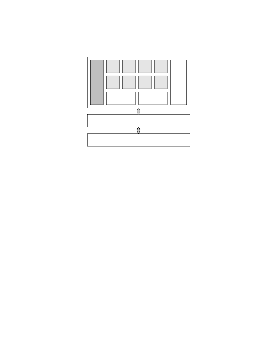
Figure 1: A schematic view of a CUDA streaming multiprocessor with 8 scalar processor
cores.

GPU contains tens of multiprocessors. A multiprocessor consists of 8 scalar pro-

cessors (SPs), each capable of executing an independent thread (see Fig. 1). The

multiprocessors have four types of on-chip memory:

• a set of 32-bit registers (local, one set per scalar processor)

• a limited amount of shared memory (16 kB for devices having Compute

Capability 1.3 or lower, shared between all SPs in a MP)

• a constant cache (shared between SPs, read-only)

• a texture cache (shared between SPs, read-only)

The amount of on-chip memory is very limited in comparison to the total

global memory available on a graphics device (a few kilobytes vs hundreds

of megabytes). Its advantage lies in the access time, which is two orders of

magnitude lower than the global memory access time.

The CUDA programming model is based upon the concept of a kernel. A

kernel is a function that is executed multiple times in parallel, each instance

running in a separate thread. The threads are organized into one-, two- or three-

dimensional blocks, which in turn are organized into one- or two-dimensional

grids. The blocks are completely independent of each other and can be executed

in any order. Threads within a block however are guaranteed to be run on a

single multiprocessor. This makes it possible for them to synchronize and share

information efficiently using the on-chip memory of the SM.

In a device having Compute Capability 1.2 or higher, each multiprocessor

is capable of concurrently executing 1024 active threads [16]. In practice, the

3

number of concurrent threads per SM is also limited by the amount of shared

memory and it thus often does not reach the maximum allowed value.

The CUDA environment also includes a software stack. For CUDA v2.1, it

consists of a hardware driver, system libraries implementing the CUDA API,

a CUDA C compiler and two higher level mathematical libraries (CUBLAS

and CUFFT). CUDA C is a simple extension of the C programming language,

which includes several new keywords and expressions that make it possible to

distinguish between host (i.e. CPU) and GPU functions and data.

3. Specific models

In this work, we study the numerical solution of stochastic differential equa-

tions modeling the dynamics of Brownian particles. The two models we con-

centrate upon are of particular interest in many disciplines and illustrate the

flexibility of the employed methods of solution.

The first model describes a single Brownian particle moving in a symmetric

periodic potential V (x) = sin(2πx) under the influence of a constant bias force
f and a periodic unbiased driving with amplitude a and frequency ω:

¨x + γ ˙x = −V

0

(x) + a cos(ωt) + f + p2γk

B

T ξ(t)

(1)

where γ is the friction coefficient and ξ(t) is a zero-mean Gaussian white noise

with the auto-correlation function hξ(t)ξ(s)i = δ(t−s) and noise intensity k

B

T .

Equation 1 is known as the Stewart-McCumber model [3] describing phase

differences across a Josephson junction. It can also model a rotating dipole

in an external field, a superionic conductor or a charge density wave. It is

particularly interesting since it exhibits a wide range of behaviors, including

chaotic, periodic and quasi-periodic motion, as well as the recently detected

phenomenon of absolute negative mobility [17, 18].

The second model we analyze is that of N globally interacting overdamped

Brownian particles, with the dynamics of the i-th particle described by:

γ ˙

x

i

= ω

i

+

N

X

j

=1

K

ij

sin(x

j

− x

i

) +

p

2γk

B

T ξ

i

(t), i = 1, . . . , N

(2)

This model is known as the Kuramoto model [19] and is used as a simple

paradigm for synchronization phenomena. It has found applications in many

areas of science, including neural networks, Josephson junction and laser arrays,

charge density waves and chemical oscillators.

4. Numerical solution of SDEs

Most stochastic differential equations of practical interest cannot be solved

analytically, and thus direct numerical methods have to be used to obtain the

4

solutions. Similarly as in the case of ordinary differential equations, there is an

abundance of methods and algorithms for solving stochastic differential equa-

tions. Their detailed description can be found in references: [20, 21, 22, 23, 24,

25].

Here, we present the implementation of a standard stochastic algorithm on

the CUDA architecture in three distinctive cases:

1. Multiple realizations of a system are simulated, and an ensemble average

is performed to calculate quantities of interest. The large degree of paral-

lelism inherent in the problem makes it possible to fully exploit the com-

putational power of CUDA devices with tens of multiprocessors capable of

executing hundreds of threads simultaneously. The example system models

the stochastic phase dynamics in a Josephson junction and is implemented

in program PROG1 (the source code is available in [15]).

2. The system consists of N globally interacting particles. In each time step

N

2

interaction terms are calculated. The example algorithm is named

PROG2

and solves the Kuramoto model (Eq. 2.)

3. The system consists of N globally interacting particles as in the previous

case but the interaction can be expressed in terms of a parallel reduction

operation, which is much more efficient than PROG2. The example algo-

rithm in PROG3 also solves the Kuramoto model (Eq. 2.)

We will now outline the general patterns used in the solutions of all models.

We start with the model of a single Brownian particle, which will form a basis

upon which the solution of the more general model of N globally interacting

particles will be based.

4.1. Ensemble of non-interacting stochastic systems

Algorithm 1

A CUDA kernel to advance a Brownian particle by m · ∆t in

time.

1:

local i ← blockIdx.x · blockDim.x + threadIdx.x

2:

load x

i

, v

i

and system parameters {par

ji

} from global memory and store

them in local variables

3:

load the RNG seed seed

i

and store it in a local variable

4:

for

s = 1 to m do

5:

generate two uniform variates n

1

and n

2

6:

transform n

1

and n

2

into two Gaussian variates

7:

advance x

i

and v

i

by ∆t using the SRK2 algorithm

8:

local t ← t

0

+ s · ∆t

9:

end for

10:

save x

i

, v

i

and seed

i

back to global memory

For the Josephson junction model described by Eq. 1 we use a single CUDA

kernel, which is responsible for advancing the system by a predefined number

of timesteps of size ∆t.

5

Algorithm 2

The Stochastic Runge-Kutta algorithm of the 2nd order (SRK2)

to integrate ˙x = f(x) + ξ(t), hξ(t)i = 0, hξ(t)ξ(s)i = 2Dδ(t − s).

1:

F

1

← f(x

0

)

2:

F

2

← f(x

0

+ ∆tF

1

+

√

2D∆tψ) {with hψi = 0, hψ

2

i = 1}

3:

x(∆t)

← x

0

+

1
2

∆t(F

1

+ F

2

)

√

2D∆tψ

We employ fine-grained parallelism – each path is calculated in a separate

thread. For CUDA devices, it makes sense to keep the number of threads

as large as possible. This enables the CUDA scheduler to better utilize the

available computational power by executing threads when other ones are waiting

for global memory transfers to be completed [16]. It also ensures that the code

will execute efficiently on new GPUs, which, by the Moore’s law, are expected to

be capable of simultaneously executing exponentially larger numbers of threads.

We have found that calculating 10

5

independent realizations is enough to obtain

a satisfactory level of convergence and that further increases of the number of

paths do not yield better results (see Fig. 5).

In order to increase the number of threads, we structured our code so that

Eq. 1 is solved for multiple values of the system parameters in a single run. The

default setup calculates trajectories for 100 values of the amplitude parameter
a. This makes it possible to use our code to efficiently analyze the behavior of

the system for whole regions of the parameter space {a, ω, γ}.

Multiple timesteps are calculated in a single kernel invocation to increase

the efficiency of the code. We observe that usually only samples taken every
M steps are interesting to the researcher running the simulation, the sampling

frequency M being chosen so that the relevant information about the analyzed

system is retained. In all following examples M = 100 is used. It should be

noted that the results of the intermediate steps do not need to be copied to

the host (CPU) memory. This makes it possible to limit the number of global

memory accesses in the CUDA threads. When the kernel is launched, path

parameters x, v = ˙x and a are loaded from the global memory and are cached

in local variables. All calculations are then performed using these variables and

at the end of the kernel execution, their values are written back to the global

memory.

Each path is associated with its own state of the random number genera-

tor (RNG), which guarantees independence of the noise terms between different

threads. The initial RNG seeds for each thread are chosen randomly using a

standard integer random generator available on the host system. Since CUDA

does not provide any random number generation routines by default, we imple-

mented a simple xor-shift RNG as a CUDA device function. In our kernel, two

uniform variates are generated per time step and then transformed into Gaussian

variates using the Box-Muller transform. The integration is performed using a

Stochastic Runge-Kutta scheme of the 2nd order, which uses both Gaussian

variates for a single time step.

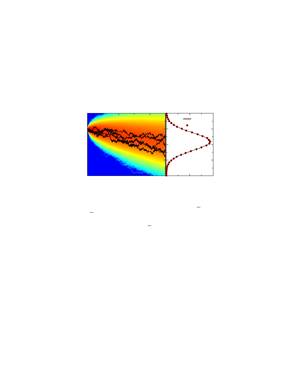
In the example in Fig. 2 we present the results coming from the simultaneous

6

−150

−100

−50

0

50

xx

0

1000

2000

tt

N = 0.5

× 10

6

GP U : 21s

0

0.0025

0.005

P (x; t = 2500)

P (x; t = 2500)

single

double

Figure 2: The ensemble of 524288 Brownian particles, modeling the noisy dynamics of phase
in a Josephson junction described by Eq. 1 is simulated for time t ∈ (0, 2000

2π

ω

) with time

step ∆t = 0.01

2π

ω

. On the left panel sample trajectories are drawn with black lines and

the background colors represent the coarse-grained (averaged over a potential period) density
of particles in the whole ensemble.

The right panel shows the coarse-grained probability

distribution of finding a particle at time t = 2000

2π

ω

obtained by means of a histogram with

200 bins. The histogram is calculated with both single and double precision on a GPU with
Compute Capability v1.3. The same calculation has also been performed on the CPU but
their identical results are not presented for clarity purposes. The total simulation times were:
20 seconds and 13 minutes on NVIDIA Tesla 1060C when using single and double precision
floating-point arithmetics, respectively. The CPU-based version of the same algorithm needed
over three hours. Used parameters: a = 4.2, γ = 0.9, ω = 4.9, D

0

= 0.001, f = 0.1 correspond

to the anomalous response regime (cf. [17]).

7

solution of N = 2

19

= 524288 independent Eqs. 1 for the same set of parameters.

The total simulation time was less than 20 seconds. In this case the CUDA

platform turns out to be extremely effective, outperforming the CPU by a factor

of 675. In order to highlight the amount of computation, let us note that the

size of the intermediate file with all particle positions used for generation of the

background plot was about 30 GB.

4.2.

N globally interacting stochastic systems

Algorithm 3

The AdvanceSystem CUDA kernel.

1:

local i ← blockIdx.x · blockDim.x + threadIdx.x

2:

local mv ← 0

3:

local mx ← x

i

4:

for all

tiles do

5:

local tix ← threadIdx.x

6:

j

← tile · blockDim.x + threadIdx.x

7:

shared sx

tix

← x

j

8:

synchronize with other threads in the block

9:

for

k = 1 to blockDim.x do

10:

mv

← mv + sin(mx − sx

k

)

11:

end for

12:

synchronize with other threads in the block

13:

end for

14:

v

i

← mv

For the general Kuramoto model described by Eqs. 2 or other stochastic

systems of N interacting particles, the calculation of O(N

2

) interaction terms for

all pairs (x

j

, x

i

) is necessary in each integration step. In this case the program

PROG2

is split into two parts, implemented as two CUDA kernels launched

sequentially. The first kernel, called UpdateRHS calculates the right hand

side of Eq. 2 for every i. The second kernel AdvanceSystem actually advances

the system by a single step ∆t and updates the positions of all particles. In our

implementation the second kernel uses a simple first-order Euler scheme. It is

straightforward to modify the program to implement higher-order schemes by

interleaving calls to the UpdateRHS kernel with calls to kernels implementing

the sub-steps of the scheme.

The UpdateRHS kernel is organized around the concept of tiles, introduced

in [26]. A tile is a group of T particles interacting with another group of T

particles. Threads are executed in blocks of size T and each block is always

processing a single tile. There is a total of N/T blocks in the grid. The i-th

thread computes the interaction of the i-th particle with all other particles.

The execution proceeds as follows. The i-th thread loads the position of

the i-th particle and caches it as a local variable. It then loads the position

of another particle from the current tile, stores it in shared memory and syn-

chronizes with other threads in the block. When this part is completed, the

8

th

re

ad

s

time

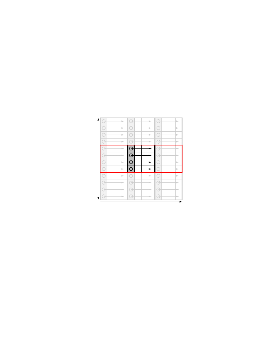
Figure 3: All-pairs interaction of 12 particles calculated using the tile-based approach with 9
tiles of size 4x4. The chosen number of particles and the size of the tiles are made artificially
low for illustration purposes only.

A small square represents the computation of a single

particle-particle interaction term. The highlighted part of the schematic depicts a single tile.
The bold lines represent synchronization points where data is loaded into the shared memory
of the block. The filled squares with circles represent the start of computation for a new tile.
Threads in the red box are executed within a single block.

9

N = 17

× 10

6

GP U : 20s

t

x

0

π

2π

0

5

10

15

20

0

0.25

0.5

0.75

P

(x

;t

)

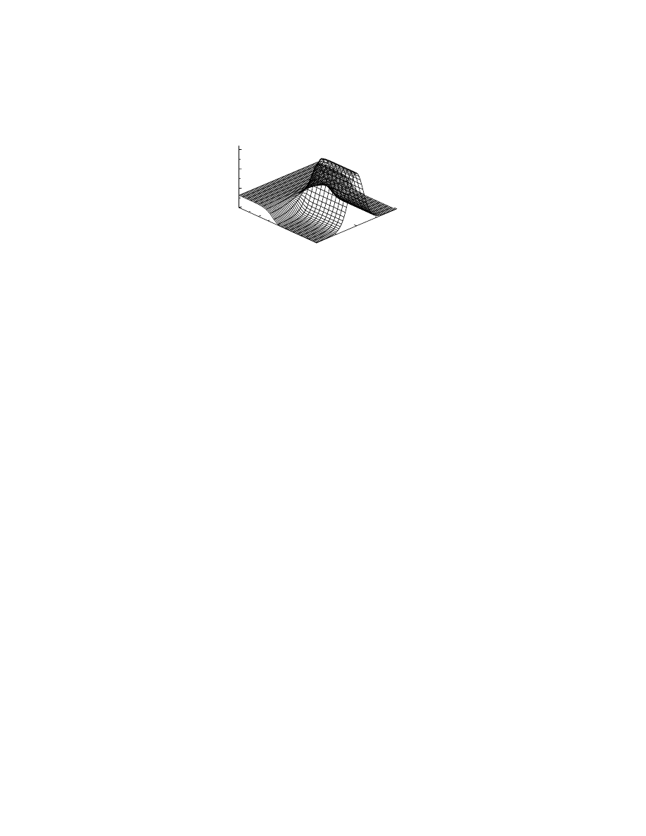
Figure 4: An example result of the integration of the Kuramoto system (Eq.

2). The time

evolution of the probability density P (x; t) is shown for ω

i

= 0, K

ij

= 4, T = 1. The density

is a position histogram of 2

24

particles. The total time of simulation was approximately 20

seconds using the single precision capabilities of NVIDIA Tesla C1060.

positions of all particles from the current tile are cached in the shared memory.

The computation of the interaction is then commenced, with the i-th thread

computing the interaction of the i-th particle with all particles from the current

tile. Afterwards, the kernel advances to the following tile, the positions stored

in shared memory are replaced with new ones, and the whole process repeats.

This approach might seem wasteful since it computes exactly N

2

interaction

terms, while only (N − 1)N/2 are really necessary for a symmetric interaction.

It is however very efficient, as it minimizes global memory transfers at the cost

of an increased number of interaction term computations. This turns out to be

a good trade-off in the CUDA environment, as global memory accesses are by

far the most costly operations, taking several hundred clock cycles to complete.

Numerical computations are comparatively cheap, usually amounting to just a

few clock cycles.

The special form of the interaction term in the Kuramoto model when

K

ij

= K = const, allows us to significantly simplify the calculations. Using

the identity:

N

X

j

=1

sin(x

j

− x

i

) =

cos(x

i

)

N

X

j

=1

sin(x

j

) − sin(x

i

)

N

X

j

=1

cos(x

j

)

(3)

we can compute two sums: P

N
j

=1

sin(x

j

) and P

N
j

=1

cos(x

j

) only once per inte-

gration step, which has a computational cost of O(N). The calculation of the

sum of a vector of elements is an example of the vector reduction operation,

which can be performed very efficiently on the CUDA architecture. Various

methods of implementation of such an operation are presented in the sample

code included in the CUDA SDK 2.1 [27]. The integration of the Kuramoto sys-

tem taking advantage of Eq. 3 and using a simple form of a parallel reduction

is implemented in PROG3.

10

In Fig. 4 we present a solution of the classical Kuramoto system described

by Eqs. 2 for parameters as in Fig. 10 of the review paper [19]. In this case we

apply the program PROG3 which makes use of the relation from Eq. 3. The

number of particles N = 2

24

≈ 16.8 · 10

6

and the short simulation time clearly

demonstrate the power of the GPU for this kind of problems.

5. Note on single precision arithmetics

The fact that the current generation of CUDA devices only implements single

precision operations in an efficient way is often considered a significant limitation

for numerical calculations. We have found out that for the considered models

this does not pose a problem. Figure 2 presents sample paths and position

distribution functions of a Brownian particle whose dynamics is determined by

Eq. 1 (colored background on the left panel and right panel). Let us note that

we present coarse-grained distribution functions where the position is averaged

over a potential period by taking a histogram with bin size being exactly equal

to the potential period. We observe that the use of single precision floating-point

numbers does not significantly impact the obtained results. Results obtained by

single precision calculations even after a relatively long time t = 2000

2π

ω

differ

from their double precision counterparts only up to the statistical error, which

in this case can be estimated by the fluctuations of the relative particle number

in a single histogram bin. Since in the right panel of Fig. 2 we have approxi-

mately 10

4

particles in one bin, the error is of the order of 1%. If time-averaged

quantities such as the asymptotic velocity hhvii = lim

t→∞

hv(t)i are calculated,

the differences are even less pronounced. However, the single and double preci-

sion programs produce different individual trajectories as a direct consequence

of the chaotic nature of the system given by Eq. 1. Moreover, we have no-

ticed that even when changing between GPU and CPU versions of the same

program, the individual trajectories diverged after some time. The difference

between paths calculated on the CPU and the GPU, using the same precision

level, can be explained by differences in the floating-point implementation, both

in the hardware and in the compilers.

When doing single precision calculations special care must be taken to ensure

that numerical errors are not needlessly introduced into the calculations. If one

is used to having all variables defined as double precision floating-point numbers,

as is very often the case on a CPU, it is easy to forget that operations which work

just fine on double precision numbers might fail when single precision numbers

are used instead. For instance, consider the case of keeping track of time in

a simulation by naively increasing the value of a variable t by a constant ∆t

after every step. By doing so, one is bound to hit a problem when t becomes

large enough, in which case t will not change its value after the addition of a

small value ∆t, and the simulation will be stuck at a single point in time. With

double precision numbers this issue becomes evident when there is a difference

of 17 orders of magnitude between t and ∆t. With single precision numbers,

a 8-orders-of-magnitude difference is enough to trigger the problem. It means

that if, for instance, t is 10

5

and ∆t is 10

−4

, the addition will no longer work

11

0

100

200

300

400

GF

LO

P

S

GF

LO

P

S

10

3

10

4

10

5

10

6

10

7

N

N

PROG1

PROG2

PROG3

C

P

U

×

10

C

P

U

×

10

C

P

U

×

10

PROG1 PROG2 PROG3

0

100

200

300

400

GFLOPSGFLOPS

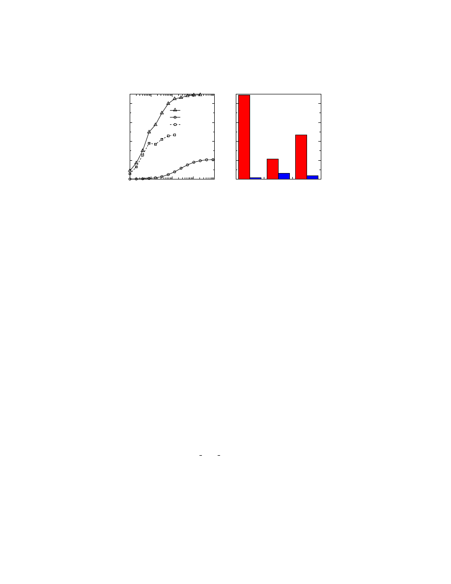
Figure 5: (Left panel) Performance estimate for the programs PROG1 -PROG3 as a function
of the number of particles N . (Right panel) Performance estimate for the programs PROG1 -
PROG3 on an Intel Core2 Duo E6750 CPU and NVIDIA Tesla C1060 GPU. We have counted
79, 44 + 6N and 66 operations per one integration step of programs PROG1, PROG2 and
PROG3, respectively.

as expected. 10

5

and 10

−4

are values not uncommon in simulations of the type

we describe here, hence the need for extra care and reformulation of some of

the calculations so that very large and very small quantities are not used at the

same time. In our implementations, we avoided the problem of spurious addition

invariants by keeping track of simulation time modulo the system period 2π/ω.

This way, the difference between t and ∆t was never large enough to cause any

issues.

6. Performance evaluation

In order to evaluate the performance of our numerical solution of Eqs. 1

and 2, we first implemented Algs. 3 and 1 using the CUDA Toolkit v2.1. We then

translated the CUDA code into C++ code by replacing all kernel invocations

with loops and removing unnecessary elements (such as references to shared

memory, which does not exist on a CPU).

We used the NVIDIA CUDA Compiler (NVCC) and GCC 4.3.2 to compile

the CUDA code and the Intel C++ Compiler (ICC) v11.0 for Linux to compile

the C++ version. We have determined through numerical experiments that

enabling floating-point optimizations significantly improves the performance of

our programs (by a factor of 7 on CUDA) and does not affect the results in a

quantitative or qualitative way. We have therefore used the -fast -fp-model
fast=2

ICC options and --use fast math in the case of NVCC.

All tests were conducted on recent GNU/Linux systems using the following

hardware:

• for the CPU version: Intel Core2 Duo E6750 @ 2.66GHz and 2 GB RAM

(only a single core was used for the calculations)

12

• for the GPU version: NVIDIA Tesla C1060 installed in a system with Intel

Core2 Duo CPU E2160 @ 1.80GHz and 2 GB RAM

Our tests indicate that speedups of the order of 600 and 100 are possible

for the models described by Eqs. 1 and 2, respectively. The performance gain

is dependent on the number of paths used in the simulation. Figure 5 shows

that it increases monotonically with the number of paths, and then saturates

at a number dependent on the used model: 450 and 106 GFLOPS for the

Eqs. 1 and 2, respectively (which corresponds to speedups: 675 and 106). The

saturation point indicates that for the corresponding number of particles the

full computational resources of the GPU are being exploited.

The problem of lower performance gain for small numbers of particles could

be rectified by dividing the computational work between threads in a different

way, i.e. by decreasing the amount of calculations done in a single thread, while

increasing the total number of threads. This is a relatively straightforward thing

to do, but it increases the complexity of the code. We decided not to do it since

for models like 1 and 2 one is usually interested in calculating observables for

whole ranges of system parameters. Instead of modifying the code to run faster

for lower number of paths, one can keep the number of paths low but run the

simulation for multiple system parameters simultaneously, which results in a

higher number of threads.

7. Conclusions

In this paper we have demonstrated the suitability of a parallel CUDA-based

hardware platform for solving stochastic differential equations. The observed

speedups, compared to CPU versions, reached an astonishing value 670 for non-

interacting particles and 120 for a globally coupled system. We have also shown

that for this kind of calculations single precision arithmetics poses no problems

with respect to accuracy of the results, provided that some kind of operations,

such as adding small and large numbers, are avoided.

The availability of cheap computer hardware which is over two orders of

magnitude faster clearly announces a new chapter in high performance com-

puting. Let us note that the development of stream processing technology for

general-purpose computing has just started and its potential is surely not yet

fully revealed. In order to take advantage of the new hardware architecture, the

software and its algorithms must be substantially redesigned.

8. Appendix: Estimation of FLOPS

We counted the floating-point operations performed by the kernels in our

code, and the results in the form of the collective numbers of elementary op-

erations are presented in Table 1. The number of MAD (Multiply and Add)

operations can vary, depending on how the compiler processes the source code.

13

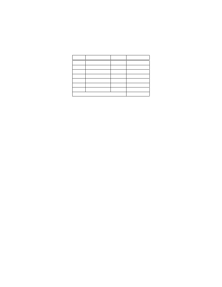
Table 1: Number of elementary floating-point operations performed per one time step in the
AdvanceSystem kernel for Eq. 1.

count

type

FLOPs totalFLOPs

22

multiply, add

1

22

11

MAD

1

11

2

division

4

8

3

sqrt

4

12

1

sin

4

4

5

cos

4

20

1

log

2

2

TOTAL:

79

For the purposes of our performance estimation, we assumed the most opti-

mistic version. A more conservative approach would result in a lower number

of MADs, and correspondingly a higher total number of GFLOPS.

The amount of FLOPs for functions such as sin, log, etc. is based on [16],

assuming 1 FLOP for elementary arithmetical operations like addition and mul-

tiplication and scaling the FLOP estimate for complex functions proportionately

to the number of processor cycles cited in the manual. The numbers of floating-

point operations are summarized in Table 1.

On a Tesla C1060 device our code PROG1 evaluates 6.178 · 10

9

time steps

per second. The cost of each time step is 79 FLOPs, which implies that the

overall performance estimate accounts for 490 GFLOPS.

In the case of PROG2 the number of operations per one integration step

depends on the number of particles N. A similar operation count as the one

presented in Table 1 resulted in the formula 44 + 6N FLOPs per integration

step.

References

[1] Reimann, P., Physics Reports 361 (2002) 57 .

[2] Kostur, M., Machura, L., Talkner, P., H¨anggi, P., and Luczka, J., Physical

Review B (Condensed Matter and Materials Physics) 77 (2008) 104509.

[3] Kautz, R. L., Reports on Progress in Physics 59 (1996) 935.

[4] Gammaitoni, L., H¨anggi, P., Jung, P., and Marchesoni, F., Rev. Mod.

Phys. 70 (1998) 223.

[5] Groot, R. and Warren, P., J. Chem. Phys. 107 (1997) 4423.

[6] McLeish, D. L., Monte Carlo Simulation and Finance, John Wiley and

Sons, 2005.

[7] Bartussek, R., Reimann, P., and H¨anggi, P., Phys. Rev. Lett. 76 (1996)

1166.

14

[8] Lindner, B., Schimansky-Geier, L., Reimann, P., H¨anggi, P., and Nagaoka,

M., Phys. Rev. E 59 (1999) 1417.

[9] Kalmykov, Y. P., Phys. Rev. E 61 (2000) 6320.

[10] Kostur, M., Internat. J. Modern Phys. C 13 (2002) 1157.

[11] Yu, J. and Lin, Y., Internat. J. Non-Linear Mech. 39 (2004) 1493.

[12] Naess, A., Dimentberg, M. F., and Gaidai, O., Physical Review E (Statis-

tical, Nonlinear, and Soft Matter Physics) 78 (2008) 021126.

[13] http://www.computermuseum.li/testpage/asci-red-supercomputer.htm.

[14] Nvidia cuda webpage, http://www.nvidia.com/object/cuda home.html.

[15] Source code of all examples can be found on http://fizyka.us.edu.pl/cuda.

[16] Corporation, N., Nvidia cuda programming guide v2.1, available from

nvidia cuda webpage,

http://www.nvidia.com/object/cuda home.html,

2008.

[17] Machura, L., Kostur, M., Talkner, P., Luczka, J., and H¨anggi, P., Physical

Review Letters 98 (2007) 040601.

[18] Speer, D., Eichhorn, R., and Reimann, P., EPL (Europhysics Letters) 79

(2007) 10005 (5pp).

[19] Acebron, J. A., Bonilla, L. L., Vicente, C. J. P., Ritort, F., and Spigler, R.,

Reviews of Modern Physics 77 (2005) 137.

[20] Mannella, R. and Palleschi, V., Phys. Rev. A 40 (1989) 3381.

[21] Mannella, R., Internat. J. Modern Phys. C 13 (2002) 1177.

[22] Sancho, J. M., Miguel, M. S., Katz, S. L., and Gunton, J. D., Phys. Rev.

A 26 (1982) 1589.

[23] Fox, R. F., Gatland, I. R., Roy, R., and Vemuri, G., Phys. Rev. A 38

(1988) 5938.

[24] Honeycutt, R. L., Phys. Rev. A 45 (1992) 600.

[25] Kloeden, P. E. and Platen, E., Numerical Solution of Stochastic Differential

Equations (Stochastic Modelling and Applied Probability)

, Springer, 2000.

[26] L. Nyland, M. Harris, J. P., GPU Gems 3 - Fast N-body simulation with

CUDA

, chapter 31, pages 677–695, Addison-Wesley Professional, 2007.

[27] Nvidia cuda software development kit, available from nvidia cuda webpage,

http://www.nvidia.com/object/cuda home.html.

15