
On the possibility of practically obfuscating programs
Towards a unified perspective of code protection
Philippe Beaucamps
∗
Éric Filiol
†
Ecole Supérieure et d’Application des Transmissions
Laboratoire de virologie et de cryptologie
B.P. 18, 35998 Rennes Armées, FRANCE
July 6, 2008
The original publication is available at www.springerlink.com
DOI: 10.1007/s11416-006-0029-6
Abstract
Barak et al. gave a first formalization of obfuscation, describing an obfuscator O as
an efficient, probabilistic “compiler” that takes in input a program P and produces a new
program O (P ) that has the same functionality as P but is unintelligible. This mean that
any result an obfuscated program can compute is actually computable given only an in-
put/output access (called oracle access) to the program P : we call such results trivial
results. On the basis of this informal definition, they suggest a formal definition of obfusca-
tion based on oracle access to programs and show that no obfuscator can exist according to
this definition. They also try to relax the definition and show that, even with a restriction
to some common classes of programs, there exists no obfuscator.
In this work, we show that their definition is inaccurate and lacks a fundamental property,
that we formalize by the notion of oracle programs. Oracle programs are an abstract notion
which basically refers to perfectly obfuscated programs. We suggest a new definition of
obfuscation based on these oracle programs and show that such obfuscators do not exist
either. Considering the actual implementations of “obfuscators”, we define a new kind of
obfuscators, τ -obfuscators. These are obfuscators that hide non trivial results at least for
time τ . By restricting the τ -requirement to deobfuscation (that is outputting an intelligible
program when fed with an obfuscated program in input), we show that such obfuscators
do exist. Practical τ -obfuscation methods are presented at the end of this paper: we focus
more specifically on code protection techniques in a malware context.
Based on the fact that a malware may fulfill its action in an amount of time which may
be far larger than the analysis time of any automated detection program, these obfuscation
methods can be considered as efficient enough to greatly thwart automated analysis and put
check on any antivirus software.
1
Introduction
Obfuscation is the process of making circuits or programs unintelligible. This article will focus
more specifically on computer programs. When developing programs, the intelligible source code
∗
philippe.beaucamps_at_loria_dot_fr
†
eric.filiol_at_esat.terre.defense.gouv.fr
1

is translated into some binary language, whose structure follows quite precisely the structure of
the source code. Thus the initial source code could be retrieved by using some common reverse
engineering techniques. Depending on the compiled language being used, this process is more
or less long and difficult but is eventually carried out if no protection measure has been taken.
Some technologies are particularly sensitive besides, like Java and .NET technologies: the source
code is compiled in a very high level byte code that is essentially a line by line binary translation
of the source code. Thus, many tools exist for both technologies, that allow decompiling such
binary codes in a matter of seconds.
Commercial programs are particularly concerned with this problem, due to the need of pro-
tection of the software. Another application of obfuscation is in virology among others. A
major concern of malware developers is to make malware undetectable by any sequence-based
detection techniques: this is achieved by making the malware polymorphic or metamorphic.
Polymorphism/metamorphism is the property of the malware of never replicating in the same
way, which means that there is an infinite number of distinct copies of the malware. Obfuscation
provides a mean for the malware to achieve or increase its polymorphism since it transforms a
program into an obscure program yet producing the same results as the initial program.
This context makes obfuscation interesting to study, at least to know if it might exist or not
and maybe to find out some obfuscation methods that might be used by the previous applica-
tions. Barak & al. [BGI
+
01] gave in 2001 a first formalization of obfuscation. They propose
a formal definition of obfuscators and their main result has been to prove that obfuscators did
not exist. They proved that this result still holds for approximate obfuscators, i.e. obfuscators
producing programs that are approximately functionally equivalent to the input program. They
also considered the case of restricting obfuscators to some specific classes of programs or circuits
and showed that, for some very common classes, such obfuscators could not exist either.
This article will aim at providing a theoretical as well as a practical framework for the study
of obfuscation methods in the general context of code protection. We will start with a theoretical
analysis of obfuscation in Section 3. By going into Barak & al’s definition in depth, we point out
that there is an inaccuracy. The proof of some of the previous impossibility results is based on
this flaw, which makes it quite relevant. We will therefore propose a new definition of obfuscators
and show that the impossibility results are still valid for our new definition.
Given these impossibility results, we will suggest relaxed definitions of obfuscators that would
allow the concept of obfuscation to be applied in some restricted way. We describe more partic-
ularly obfuscators whose efficiency can be limited in time. These τ -obfuscators require that the
obfuscation remains effective at least for time τ .
Obfuscation must be considered furthermore along with its reversing process, that is to say
deobfuscation: we will propose a formal definition of deobfuscation in Section 4 and give some
basic results and suggest.
We will finally get into more practical details in Sections 5 and 6 by first describing some
obfuscation methods that might comply with our relaxed requirements of obfuscation and then
describing how a malware could use τ -obfuscation for stealth and possibly polymorphism pur-
pose. In this context, we propose a unified approach of code protection in which obfuscation
is considered along with other techniques (polymorphism/metamorphism, light code armouring,
encryption).
2
Definitions and notations
2.1
Notations
Let us consider two algorithms A and B.
2

We denote by
|A| the size of A and by t (A (x)) its running time on input x (provided that A
halts on input x).
We say that A is
PPT or that A ∈ PPT if A is a probabilistic polynomial time algorithm
[Pap95, §11.2].
Let us denote by A(x)
ր the fact that the computation of A on an input x never halts (and
consequently never yields a result).
A
and B are said to be functionally equivalent, which we denote by A
≡ B, if and only if
they produce the same results on their inputs. If A and B are defined on
D
A
and
D
B
, then:
D
A
=
D
B
∀x ∈ D
A
,
B
(x)
ր if A(x) ր
B
(x) = A(x) otherwise.
Let us consider that A and B are probabilistic algorithms. Given two inputs x and y, we
denote by Pr [A (x)]
≈ Pr [B (y)] the fact that the distributions of outputs of A and B on their
respective inputs x and y are the same, up to a negligible difference.
A
(1
t
) refers to the algorithm A limited in its running time by time t:
∀x ∈ {0, 1}
⋆
, A x,
1
t
=
A
(x)
if A(x) can be evaluated in less than time t
⊥
otherwise (the function is undefined on input x)
T C
0
programs are polynomial programs, which means that their running time is polynomial
in the size of the input. If P is a T C
0
program, then there is a polynomial p such that:
∀x, t(P (x)) = p(|x|)
2.2
Functional decomposition
Let f :
{0, 1}
p
→ {0, 1}
q
be a function, with p, q > 0. The function f has a unique functional
decomposition in f
0
and f
1
that we note: f = f
0
#f
1
. f
0
and f
1
are defined as follows:
f
0
:
{0, 1}
p
−1
→ {0, 1}
q
x
7→ f(0.x)
f
1
:
{0, 1}
p
−1
→ {0, 1}
q
x
7→ f(1.x)
where 0.x is the result of the concatenation of 0 and x.
2.3
Obfuscation
We say that we have an oracle access to a program P when we do not have access to a program’s
description of P but, for any input x, we have access to P (x) in a polynomial time (in the size
of P ). Oracle access to P is therefore equivalent to an input/output access to P . An algorithm
A
having an oracle access to P is denoted by A
P
. Note that the only possible queries are
input/output ones since we have no access to a program’s description of P .
Let Ω be the set of obfuscators (as we will define them in this article) and let Π be the set of
programs that we want to obfuscate using obfuscators of Ω. Ω is the set of deobfuscators
1
and
Ω
O
is the set of deobfuscators with regards to a given obfuscator
O ∈ Ω.
1
The concept of deobfuscation will be exposed in Section 4.
3

Let R be a result on programs of Π. Typically, R is in fact a property of Π and thus can be
defined as a predicate. We say that R is trivial if it can be computed for a program P by simply
querying P on some specific inputs.
Thus an obfuscator is expected to hide any non trivial result. In other words, any result an
adversary can compute from an obfuscated program is actually trivial. Barak & al. gave the
following definition:
Definition 1.
A probabilistic algorithm
O is an obfuscator if it satisfies the following properties:
• Functionality: for any P ∈ Π, P and O (P ) compute the same function.
• Polynomial slowdown: for any P ∈ Π, the running time and size of O (P ) are at most
polynomially larger than the size and running time of P .
• "Virtual black box": for any adversary A ∈ PPT , there is a simulator S ∈ PPT such
that:
∀P ∈ Π, Pr [A (O (P ))] ≈ Pr
h
S
P
1
|P |
i
The second condition is rather wide and in practice, we would require that the runtime of
the obfuscating program is simply linear in the running time of the source program. Since the
slowdown property aims at defining the efficiency of the obfuscator, it is completely up to choice.
From an intuitive point of view, the “Virtual black box” property simply asserts that anything
that can be efficiently computed from
O (P ) can also computed given oracle access to P . Thus
any property that may be computed is necessarily trivial.
Probabilities are taken over the coin tosses of
O, A and S.
An obfuscator is said to be efficient if it runs in polynomial time (in the size of the input
program).
3
New formalization and impossibility results
3.1
Barak & al’s results
Barak & al proved in particular that obfuscators, as they had formally defined them, did not
exist. We will detail the proof of this result later in this section. Let us start with the following
strong implication, that was implicitely expressed in Barak et al.’s paper.
Proposition 1.
No information can be hidden in a program, using Barak & al.’s obfuscators.
Proof.
The proof is a generalization of the proof of the Theorem 4.12, in Barak & al.s’ paper.
Barak & al. define among others a set
H of totally unobfuscatable functions. Let f ∈ H be
one of those functions.
H requires the existence of a result π on f such that, when given oracle
access to f , π(f ) yields a pseudo-random result when f is pseudo-randomly chosen in
H. H also
requires the existence of an algorithm A such that, for any program Q that computes f , then
A
(Q) computes f . Barak & al show that
H exists (H being infinite).
Let us denote this information by R.
Now define program P by :
∀x ∈ {0, 1}
∗
, P
(x) = (f (x), π(f )
⊕ R)
where f is such an unobfuscatable function.
This program P returns a couple of values that gives us no information on R when given
oracle access to P (since oracle access to P means oracle access to f and π(f ) is pseudo-random
4

in this case). Yet, for any obfuscation
O (P ) of P , we have access to a function computing f (by
simply keeping the first value): thus we can compute f itself, using A, thereby allowing us to
compute π(f ). Eventually, we are able to compute R.
Since
H is infinite, there is also an infinity of such programs P .
Barak & al. applied this result to private-key encryption schemes among others, proving that
there exist such schemes where the key can not be retrieved by oracle access though it can be
retrieved when possessing any representation of this (obfuscated) scheme.
This result already illustrates a lack in the previous definition of obfuscators. Let’s get into
more details with Barak & al’s main impossibility result.
The proof relied on the decomposition of an input program P into programs P
1
and P
2
: P =
P
1
#P
2
. Functionalities of P
1
and P
2
are preserved by any obfuscation, since the functionality
of P is preserved. Let us now consider an adversary A that computes, on the input program P ,
P
1
(P
2
). In the specific case of P
1
testing a functionality of P
2
, this result is preserved by any
obfuscation: for any obfuscator
O ∈ Ω, Pr[A(P )] = Pr[A(O (P ))].
We see that, since P
1
tests a functionality of P
2
, it might be difficult to compute this result
with only an oracle access to P . First let’s note that oracle access to P means oracle access to
P
1
and P
2
. Now we shall remember that the simulator S is defined for a given adversary A but
for any program P : thus we do not previously know what computes neither P
1
, nor P
2
. And we
cannot emulate P
1
since we only have an input/output access to it: the only way to compute
the result is to compute P
1
on an input. And this input must be a program description of P
2
,
to which we also only have an input/output access. Hence, we see that no algorithm S will be
able to simulate A.
In Barak & al’s paper, two random values α and β are considered: P
1
tests whether P
2
(α)
equals β. Since α and β are not predefined and cannot be guessed by oracle access to P , no
generic simulator can be defined. So, if we consider the case of P
2
such that P
2
(α) = β, with
O (P ) = P
1
#P
2
, then A (
O (P )) will always return 1 though S is unable to compute the result
given oracle access to P .
3.2
New formalization
The proof of this impossibility result points out an inaccuracy of the previous definition. Consider
that you have in your hands a perfectly obfuscated program, without wondering if there is an
obfuscator capable of producing it. Then, should we really be unable to compute the previous
result? Although the program is perfectly obfuscated, we have nonetheless a program Q that is
functionaly equivalent to P . So we are able to decompose it into Q = Q
1
#Q
2
and to compute
Q
1
(Q
2
). Thus, whatever the obfuscation, this result cannot be hidden, though the current
definition of obfuscators requires it.
What should be taken into account is that an obfuscator does not hide a program’s description.
We address this lack by defining oracle programs. They represent perfectly obfuscated programs,
as we just mentioned one in the previous paragraph. More formally, we give the following
definition of oracle programs:
Definition 2.
For any program P
∈ Π, we define an oracle program ˙
P as a program that is
functionally equivalent to P but that can only be accessed in an oracle way.
Note that such programs have a purely formal interest: their use does not require any pre-
liminary proof of their existence. There is in particular no equivalence between their existence
and the existence of obfuscators. Although the existence of (ideal) obfuscators would give us a
mean of producing such programs, being able to produce oracle programs might rely on some
5

exponential time algorithm or some black box access to an algorithm, which is incompatible with
the basic requirements of an obfuscator.
Given a program P and its associated oracle program ˙
P, ˙
P is an oracle program of any
program Q functionally equivalent to P .
˙
P should therefore be seen as an equivalence class
containing all programs functionally equivalent to P , hence the notation.
We should now use oracle programs in the definition of obfuscators, by basically requiring
that obfuscated programs behave like oracle programs:
Definition 3.
A probabilistic algorithm
O is an obfuscator if it satisfies the following properties:
• Functionality: for any P ∈ Π, P and O (P ) compute the same function.
• Polynomial slowdown: for any P ∈ Π, the running time and size of O (P ) are at most
polynomially larger than the size and running time of P .
• "Virtual black box": for any adversary A ∈ PPT , there is a simulator S ∈ PPT such
that:
∀P ∈ Π, Pr [A (O (P ))] ≈ Pr
h
S
˙
P, 1
|P |
i
We intuitively expect that such obfuscators will not exist either: we will show this result
latter in this section. Thus, we should try to adopt a relaxed definition of obfuscators.
In a first approach, we could require that only some results are hidden. In other words, we
should allow some non trivial results to be computed, although requiring other non trivial results
to be hidden. But then on what basis should we consider that a result is not important enough to
require its concealment? Actually, we could restrict the obfuscation to one requirement: require
that no deobfuscation can be performed from the obfuscated program. But this requires a solid
formalization of deobfuscation, which is all the more difficult as some results can usually be
irreversibly hidden. This will be discussed in section 4.
In a second approach, we could require that the obfuscation remains effective at least for a
certain time. In other words, we allow non trivial results to be computed but not in less than
a certain time τ . We call τ -obfuscators, obfuscators with such a requirement. τ -obfuscators are
defined in the same way as obfuscators except for the virtual black box property:
Definition 4.
A probabilistic algorithm
O is a τ-obfuscator if it satisfies the following properties:
• Functionality: for any P ∈ Π, P and O (P ) compute the same function.
• Polynomial slowdown: for any P ∈ Π, the running time and size of O (P ) are at most
polynomially larger than the size and running time of P .
• "Virtual black box": for any adversary A ∈ PPT , there is a simulator S ∈ PPT such
that:
∀P ∈ Π, Pr
h
A
O (P ) , 1
τ
×t(O(P ))
i
≈ Pr
h
S
˙
P, 1
|P |
i
This property states that any result that can be computed in less than time τ
× t (O (P ))
— where t (
O (P )) is the time needed to obfuscate P — is actually computable from an oracle
program of P .
We could actually restrict in a first time the τ -requirement to deobfuscation. In other words,
a τ -obfuscator is required to prevent deobfuscation in a time less than τ
× t(O(P )). We will
show that, unlike the previous obfuscators, such τ -obfuscators do exist. Section 6 will describe
techniques that efficiently implement the τ -obfuscation concepts. We consider as an open problem
to determine whether τ -obfuscators exist in the general case (i.e. without restricting the τ -
requirement to deobfuscation).
6

3.3
Impossibility results
We show that obfuscators do not exist; in other words, there is at least one non trivial result
that can be hidden by no probabilistic algorithm.
Proposition 2.
Program obfuscators do not exist, as defined with respect to Definition 3.
Proof.
Let us first expose some preliminary considerations.
Consider a program P and an input x, this program performs several computations to even-
tually yield an output P (x). What we are interested in is the way the program computes this
result and thus we are interested in obfuscating these computations: this obfuscation might insert
some intermediary steps like decompressing or decrypting some code before executing it. These
steps could be performed beforehand and would lead to an executable code that performs the
initial computations.
We first consider this executable code only, i.e. we consider that it can be retrieved by an
algorithm, through a more or less long process.
Code of computer programs consists of simple arithmetic computations, function calls and
more complex branches that define conditional jumps or loops. These branches make the global
structure of the program.
We show that the global algorithmic structure of an obfuscated program is constrained by its
initial algorithmic structure.
Let us consider this structure. Since it is valuable information on the program’s algorithm,
this structure should be obfuscated as well. Thus an obfuscator should produce a program with
an independent structure that still yields the same results. Yet we show that an obfuscator
cannot hide this structure and preserve the program’s functionality.
In order to produce a fully independant program, an obfuscator will have to be aware of what
the initial program computes. Determining this is undecidable.
Let us consider an algorithm performing this abstraction. It would have to read the program
in a linear way. When faced with structures that might result in a non termination behaviour,
being able to interpret their result would mean being able to decide of their termination. Thus,
any representation of these structures would have to consider them in an "atomic" way.
Note that this result still holds when restricting to programs that always halt, since such
programs are structurally indistinguishable from programs that do not necessarily halt.
Thus an obfuscator will have to produce a program, based on its linear interpretation of the
initial program, hence preserving its global structure. This global structure refers precisely to
these structures that are responsible for non termination behaviours, namely the loops (in their
semantic meaning).
More specifically, this means that complex computations will always be performed in the
same way as they were in the original program. Note that simple computations might of course
be obfuscated and some code might be added that complicates that structure. Yet, when faced
with loops whose number of iterations is unknown, the obfuscator will have no other choice but
to produce a similar loop in the obfuscated program. These very loops are the ones responsible
for the non termination of programs : being able to interpret the computations of such loops
would mean being able to decide of programs’ termination.
Thus the proof relies on this more informal result :
Proposition 3.
There is no algorithm that can interpret the functionality of every program.
The reader will probably note that Proposition 3 is somehow a reformulation of Rice’s The-
orem.
7

Proof.
If this were the case, this algorithm would be able to figure out, on an algorithm-
independant level of representation, what a program computes and thereby tell if this program
halts or not on a certain input. Since the halting problem is undecidable, such an algorithm does
not exist.
This result actually comes from the fact that, since an obfuscator must preserve the func-
tionality of the input program, the output program must not halt on inputs where the input
program does not halt. And since the obfuscator can not determine where the input program
does not halt, it has to reproduce exactly the weaknesses of the input program that would be
responsible for a non-halting behaviour. These weaknesses come from the complex structures of
the input program, like infinite loops. Thus this loop structure – considering only loops whose
number of iterations is not known in advance – must be preserved as it is.
Consider for instance a loop, whose number of iterations cannot be predicted, then an obfus-
cator cannot tell whether this loop will always exit at runtime: it will therefore have to produce
a loop which performs the same computations and might never exit.
Note that this proposition too still holds when restricting to programs that always halt
(indistinguishability of programs).
This result rules out a serious lead since ideal obfuscation would be able to produce some
random independent program that computes in a different and obscure way the same results.
We know that we will not be able to modify the way results are computed but that we can
try to obfuscate sequences of simple computations and to insert code that makes the global
algorithmic structure look more confused, though it remained untouched. Section 5 will present
some methods achieving this, while usual obfuscation methods already exist, that are described
in [CTL97].
4
Deobfuscation
When trying to define new obfuscation methods, the first consideration is about reversing these
methods. This reversing process is called deobfuscation. Thus, when defining a formal framework
for obfuscation, it is also interesting to try to define one for deobfuscation as well.
Deobfuscation can be apprehended as the transformation of some obscure program into a
more intelligible program, which is functionally equivalent to the input program. More formally,
this means producing a new program on which results that were hard to compute on the initial
program become easier (in terms of complexity) to compute on this new program. In other
words, non trivial results that were hidden by the obfuscation must be computable from the
deobfuscated program. The size and running time of the deobfuscated program are necessarily
polynomial in the input size and running time, otherwise it would not be intelligible.
As for efficient obfuscators, we say that a deobfuscator is efficient if it runs in polynomial
time in the input program’s size. Then, if obfuscators existed, in their purest definition, we could
show unsurprisingly that deobfuscators cannot be efficient. Otherwise, if you consider a result
that is revealed by the deobfuscation, it could have been computed in polynomial time from the
obfuscated program by first deobfuscating the program.
To formally define deobfuscation, we state that a deobfuscator must satisfy an intelligibility
property. Thus, on the basis of Barak & al’s definition, we say that:
Definition 5.
A probabilistic algorithm D is a deobfuscator if it satisfies both following proper-
ties:
• Functionnality:
∀O ∈ Ω, ∀P ∈ Π, D (O (P )) ≡ P
8

• Intelligibility:
∀O ∈ Ω, ∀R ∈ PPT ,
∃T ∈ PPT s.t. t(T ) = O(t(R)) and (∀P ∈ Π, Pr [T (D(O (P )))] ≈ Pr [R (P )])
Probabilities are equal up to a negligible function µ
(|P |).
Note that a deobfuscator can be defined relatively to a given obfuscator
O, in which case we
would denote this deobfuscator by
O.
More informally, the intelligibility property states that any non trivial result that can be
computed from the unobfuscated program P can also be computed in approximately the same time
from the deobfuscation of any obfuscation of P
.
As we suggested it, we show that:
Proposition 4.
Efficient deobfuscators do not exist, with respect to our definition or to Barak
& al.’s definition of obfuscators.
Proof.
Let us consider an obfuscator
O ∈ Ω and a deobfuscator O ∈ Ω
O
. Let R be a non trivial
result on programs P of Π.
From the definition of deobfuscators, we infer the existence of an algorithm T computing
the same result on
O (O (P )). Let A be an adversary that computes, for an input obfuscated
program
O (P ): A (O (P )) = T O (O (P ))
= R (P ).
Then, from the definition of obfuscators, we deduce that A computes a trivial result of
O (P ),
which means that R(P ) itself can be trivially computed
2
, which contradicts the hypothesis that
R
is a non trivial result.
This definition of deobfuscators is not actually accurate enough. It does not take into account
the existence of irreversible obfuscation methods. A common obfuscation method for instance
consists in scrambling the names used in programs — since these names give information on the
structure of the code: such a method is irreversible. This question remains open and might be
subject to further research.
5
Practical obfuscation methods
The results that were exposed up to now allowed us to exclude some leads from the research of
obfuscation algorithms. Our impossibility result showed in particular that an obfuscator could
not modify the global algorithmic structure of a complex program.
5.1
Program’s representation
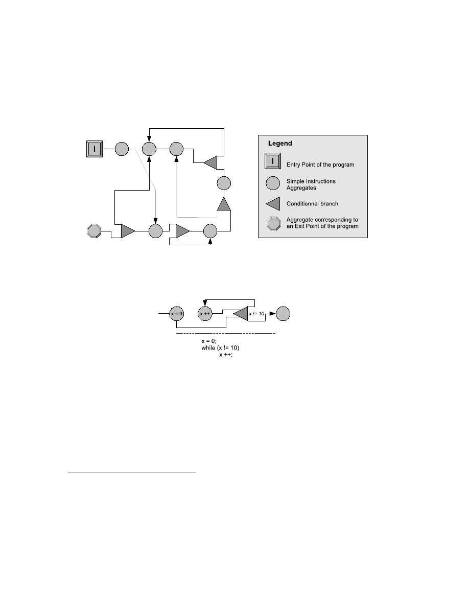
A computer program is represented as a graph, with one initial state and one or more final states.
Each vertex is a simple instruction or a conditional branch: inconditional jumps are eliminated
since connecting a vertex to an inconditional branch is equivalent to connecting the vertex to
the target of this branch.
Then we define aggregates of simple instructions by gathering together successive simple
instructions (edge contraction), whose first one only can be the target of a branch. Such simple
instruction aggregates will be denoted by the acronym SIA. There is an optimal structuration
2
Note that, in the case of Barak & al.’s definition, oracle access to P is equivalent to oracle access to O(P ). In
the case of oracle programs, we already noticed that two functionally equivalent programs share the same oracle
program (hence the notation).
9
of the program into SIAs and conditional branches: we will work on the basis of this optimal
structuration
3
It is worth noticing that a reachable instruction (from any other instruction in the graph)
does not necessarily mean it is an executable instruction. The actual execution flow may never
pass through a given instruction. This point is essential as far as Proposition 6 is concerned.
Figure 1 gives an example of the graph representation of a program. Notice, among the
miscellaneous used symbols, the conditional branches with one or more inputs and two outputs:
we might write the condition they test between these two outputs.
Figure 1: Example of a graph representation of a program
Figure 2: Sample code representation
The last step in extracting the structure of the program is to identify the loop structures.
This will allow us to determine the skeleton of the program. We can afterwards test whether a
loop has a fixed number of iterations or a variable one: in the second case, we will have to keep
the same structure for this loop (except for some basic obfuscation methods that might split the
loop into several loops or else). Some of these loops might overlap or interlock: the diagram in
figure 1 contains several loops, some of them overlapping or being interlocked. To determine this
loop structure, we can use the following algorithm, whose complexity is in O(
|P |) for a program
P
.
3
Such a representation is similar to control flow graphs or flowchart techniques.
10

We start from the entry point of the program and we explore all possible paths. If a path
crosses back one of its current vertices, then we have identified a loop. If a path crosses a vertex
that was already explored, then we stop the exploration of this particular path: indeed, if there
was to be a loop going through this vertex, then the exploration of this vertex will or would have
already identified it. There will be consequently at most
|P | visited vertices, hence a complexity
in O(
|P |)
4
.
5.2
Obfuscation options
The most basic targets of obfuscation are SIAs, as well as loops with a fixed number of iterations.
We will from now on consider only loops whose number of iterations is not fixed and previously
known.
Whenever such a loop is reached, the obfuscated program has to contain a loop, that performs
at least the computations of the initial loop. If an SIA precedes this loop and if its execution
is independent of the loop execution, then it can be moved in such a way that it is executed
during the execution of the loop — but not after the loop, since we do not know if the loop will
terminate. The same is true of instructions that follow the loop, since they are to be executed
only when the loop terminates. However, we can consider the case of programs that always
terminate: successive blocks with independent execution can then be mixed up. Note that we
can also split up the SIAs into several SIAs in order to have more freedom in our obfuscation
options.
Whenever two loops overlap in the initial program, they might be executed alternatively.
Thus we can choose between two approaches. Either we keep the overlapping, or we separate the
two loops, by replicating the common instructions block and updating the branching instructions
they contain: if a branch targets a common instruction, then it should be updated to target the
equivalent replicated instruction in the current loop. In the first case, the obfuscation of both
loops must be carried out simultaneously, while in the second case we can obfuscate in separate
ways the two common instructions blocks.
Single loops can also be obfuscated by splitting a loop into several partial loops and obfus-
cating each partial loop in a different way. The successive execution of all partial loops would
be equivalent to the execution of the unobfuscated loop, though being different from one an-
other. We could also insert new instructions between those loops and cancel the effects of these
instructions afterwards — provided that we are certain that these cancellation instructions will
be really reached.
5.3
Obfuscation methods - Targeted obfuscation
There are basically two approaches for obfuscation. Either you plan to puzzle a deobfuscator, or
you plan to puzzle an analyst (who might have executed a deobfuscator prior to beginning anal-
ysis). Both approaches will rely on two types of obfuscation methods: reversible and irreversible
methods.
Irreversible methods are quite a common use in current obfuscators. They can modify names
of functions or variables, replace function calls by the function code itself, etc. Hash functions can
also be used to implement such irreversible methods: if you store the hash value of a password,
then you will still be able to check up the validity of a password without revealing it. We can
use this method in comparisons to constant values for instance
5
.
4
Actually, |P | refers here to the number of states in the graph representation of this program, knowing fur-
thermore that some of these states are simple instructions aggregates.
5
Note that using hash functions means that there is a risk of collision, since a hash function is not injective.
11

Reversible methods refer to methods such that we can work out an intelligible, yet equivalent,
code. Note that we do not require of such obfuscation methods that their effects be cancelled
and the initial code restored: this would be meaningless since you can always slightly change the
initial code without changing the obfuscated code. Obfuscation methods that were described
in section 5.2 — which consisted in the reorganization of the loops structure — are usually
reversible and we are therefore interested in the time needed to restore the loops structure after
obfuscation.
The following sections will describe several obfuscation methods. We first think of obfuscation
with code insertion. This consists in the insertion of useless code into the program. It can either
be dead code, which means code that is never to be executed, or it can be code that can actually
be executed but whose effects are void or cancelled afterwards. We also describe the obfuscation
of the basic structure of programs, and more specifically methods to obfuscate boolean tests.
After the use of such methods, the output program should be once more obfuscated to conceal
as much as possible the use of these methods (since they might insert some predefined template
sequences of instructions).
5.3.1
Obfuscation with dead code insertion
Dead code insertion can be achieved using any valid code. The insertion point must then be
coherently chosen, since a deobfuscator will easily eliminate any code that cannot be reached from
the entry point of the program. Dead code cannot therefore be inserted after an inconditional
branch (goto) or a return instruction (return) without any branch pointing to the code: if there
is a branch pointing to this code, the branch must also be accessible from the entry point and so
on. Actually, a deobfuscator will basically keep all paths that start from the entry point of the
program. However, if we consider that code and data are mixed up and cannot be distinguished,
this code will not be deleted, though it will not appear either in any generated source code, which
makes this insertion useless.
Dead code has to be reachable though it must never be executed. We will therefore rely on
the following results, to implement code insertion:
Proposition 5.
The problem of knowing whether a piece of code is executed, for a given input,
is undecidable.
Proof.
This problem is actually a reformulation of the halting problem.
Let us proceed by reductio ab absurdum. We assume that this problem is decidable. Thus
there exists an algorithm A that can tell whether, for a given input x, a piece of code is reached
during execution of a program P .
Then applying A to every return instruction of P enables us to decide whether execution of
P
terminates on input x. Hence a contradiction.
Now we can establish a more general result.
Proposition 6.
The problem of knowing whether a piece of code is ever executed is undecidable.
In other words, there is no algorithm (whatever its complexity) that can tell with certainty
if a piece of code is dead code or not.
Thus, there is a very low probability that the functional equivalence is not fulfilled. However, let us consider the
case of a loop on a variable that is incremented from 0 to N . If N is small, then the functional equivalence will
be met with probability 1, whereas a larger N will make the functional equivalence fail with probability 1.
12

Proof.
We use the previous result.
Given a program P and an input x, we consider the equivalent program Q that is the spe-
cialization of P for its input x. Such a program Q can be seen as the program P where the input
parameter was turned into a variable initialized to x. The existence of Q is proved by Keene’s
iteration theorem (s-m-n theorem [Kle38]).
Applying proposition 5 to the program Q proves the result.
Note that this proposition could have been proven by simply using Cantor’s diagonal method.
Suppose that there exists an algorithm A deciding our problem. Then define program P and
include in it a piece of code that is executed only if A(P ) returns false. Then if A(P ) returns
true, we never execute the piece of code and it should therefore return false. However if it returns
false, we execute the piece of code, hence the contradiction.
Yet, obfuscation using dead code is not so easy because obfuscators will use predefined tech-
niques to insert dead code: a deobfuscator might try to locate some of these techniques into the
code in order to identify dead code. And, if not complex, such a method will be easily reversed
by an analyst.
Now let us consider such a dead code. Since it must never be executed but yet has to be
reachable, it will have to be the target of a conditional branch that always fails. Thus, the
less trivial the condition will be, the more undetectable the dead code will be. The condition
must test the value of some program variable, otherwise an obfuscator would only need to run
the test once to identify the dead code. So, to locate dead code, a deobfuscator will have to
either rely on the detection of known methods, or to be aware of the used variables’ values when
reaching the condition. The second technique will be made harder to use depending on the way
the variables are assigned (this must be complex and scattered among the code), whereas the
first technique might be harder to detect if the condition is furthermore complex — possibly
randomly generated.
We will use simple conditions that will test the value of a program variable x. Prior to this
test, we initialize x to a random value, by using a loop with a random number of iterations. A
deobfuscator must not be able to tell that the loop has actually a fixed number of iterations. To
achieve this, we use hash functions to compare the value of a variable to the expected value: this
allows us to hide this expected value. Thus, we propose the following code template:
h is a hash function.
Choose N randomly in a reasonable range.
Compute A = h(N) and B = h(2 * N).
Write in the obfuscated program:
int x = 0;
for (int i = 0; h(i) != A; i ++) {
x += 2;
}
if (h(x) != B) {
/* execute dead code */
}
When the loop exits, x contains the value 2
∗ N and thus the test always fails. Since N is not
stored in clear and since a deobfuscator cannot trivially guess the number of iterations of the
loop, an external observer will either assume that h(x) really equals B or will have to execute
13

the loop
6
. This solution is actually quite weak since, once the loop has been executed, we can
determine with certainty whether the code is dead or not. This is due to the fact that a complex
enough observer will notice that x and i are always initialized to the same value, just before the
loop.
Then a new solution would be to initialize x and i at the beginning of the program and to
possibly use in the obfuscated code the current values of x or i, i.e. without resetting them.
But x and i will keep getting larger and a time will come when no loop will ever execute. To
avoid this, we can add a conditional branch (on x and i) inside the loops and target it to a set of
instructions resetting x and i to random values. The loop might thereby be partially executed,
depending on the current values of x and i: as a result, these values will not be known in advance.
Thus, it will be a lot harder for a deobfuscator to prove that, when the loop terminates, x
has always the same value which prevents the dead code to be executed. Besides, this solution
reduces the performance impact since loops might be partially executed.
Here is a new code template for this obfuscation method:
Compute C = h(j), where j is randomly chosen in [0..N-1].
x and i are initialized at the beginning of the program (or function).
for (; h(i) != A; i++) {
if (h(i) == C)
goto lInsertionPoint;
x += 2;
}
if (h(x) != B) {
/* Set x and i to random values: */
x = rand(); i = rand();
/* Execute the dead code. */
goto lInsertionPoint;
}
/* Reset x and i:
* x = i = 0;
*/
lInsertionPoint:
/* Resume initial code’s execution */
A further method to deter an obfuscator from running the loop (with for instance the initial
values of x and i, which are 0) could use a dependency of the number of iterations in the value
of x. But a weakness will nonetheless remain, since a deobfuscator that would have identified
the trick can always run the loop with x and i reset to their initial values. Then introducing a
dependency in x would be of no interest, in the purpose of making x and i pseudo-unpredictable.
Note that an obfuscation of the final test can also be achieved, to make the dead code more
undetectable. Such methods will be described in the upcoming paragraphs. The code can
also be obfuscated with other techniques described in this document or in the literature about
obfuscation (see [CTL97] for instance).
6
However, there is still a small risk that h(i) equal A for i 6= N and thus that the dead code block be executed.
This risk can be ignored if we authorize the obfuscator to generate an invalid program with small probability
(which could be indeed allowed in the case of viruses for instance).
14

5.3.2
Obfuscation with void code insertion
Obfuscation with code insertion can also consist in the insertion of code which has actually no
effect on the program’s behaviour. We call such a code void code. Unlike dead code, void code
is really executed.
Void code must also be undetectable, meaning that a deobfuscator should not be able to
tell that this code is useless. However, our main advantage is that we know the location of this
useless code, while a deobfuscator has no clue about where to look for void code. This makes
void code insertion quite powerful.
Void code is implemented in the same way in Turing machines or in computer programs.
In the case of Turing machines, for instance, the read/write head must move on the tape
without modifying it or by cancelling the modifications afterwards and it must eventually come
back to its initial position. However, this code can modify the tape if it is certain that the
modification will have no impact on the expected behaviour of the program. The program might
access the modified locations of the tape afterwards, provided that we control its behaviour (for
instance, if the code using it was inserted by ourselves).
Similarly, in the case of computer programs (assembler programs), modifications due to void
code must have no impact on the further execution of the program. These modifications can
affect the memory or registers. In the case of memory, an obfuscator cannot predict if a memory
location is used by the program or not: the memory modified by void code must therefore have
been explicitely allocated by some inserted code. In the case of registers, the registers must not
be used anywhere else than in obfuscator-specific code. Any other modification must be cancelled
by the void code.
To be more powerful, the void code should be splitted up into several chunks that are scattered
in the code. This would make the detection process much harder, which is all the more interesting
as such methods would certainly use predefined void code templates.
5.3.3
Obfuscation with code duplication
We can also think of duplicating existing code and obfuscating each duplicate in a different way.
Then, we insert a test which leads to the execution of any of these duplicates. We actually have
a great deal of latitude for the test, since, whatever the result, the initial code will be executed
as expected.
5.3.4
Obfuscation with code insertion: conclusion
These methods insert code that often match some predefined template. Thus, as we told before,
the inserted code should be obfuscated afterwards with other techniques, to conceal it more
efficiently. Inserting code means also choosing specific locations where to insert it. This choice
should not be made at random since, for instance, if the code is inserted in deep loops, then the
performance impact will not be tolerable.
Yet some positions might be more propitious for code insertion. For instance, when a loop is
splitted up into several parts, code could be inserted between these parts to make the detection
of the splitted loop harder. Also, when some duplication process is used, inserting code in the
duplicates can help in making the duplicates harder to detect. This could be used for instance
when replacing function calls by a direct execution of the function body.
Finally, this obfuscation method should be applied before any other method, to help its
concealment. It should also be used with other obfuscation processes (like the ones duplicating
code).
15

5.3.5
Obfuscation of the conditional structure
The graph representation of programs use SIAs and conditional branches. These conditional
branches provide relevant information on the program’s behaviour and it would be interested to
obfuscate them as well. We describe two ways to achieve this. We could either obfuscate the
condition itself, i.e. make it complex enough to be hardly intelligible. The performance impact
would be likely to be slight, but this obfuscation would not be very strong. We could also hide
which code is executed regarding which value of the condition. This means that the program
would only be able to tell at runtime which code is to be executed if the condition is true.
We use therefore the code insertion methods’ ideas and propose the following code template:
h is a hash function.
<cond> is the tested condition.
If <cond> is true, then <block1> is executed, otherwise <block2> is executed.
Choose N randomly in a reasonable range.
Choose alpha randomly in {0, 1}.
Compute A = h(N), B = h(2 * N + alpha),
C = h(j), where j is randomly chosen in [0..N-1], and D = h(2 * j + alpha).
i and x are initialized to 0 at the beginning (of the program or the function).
Write in the obfuscated program:
int comparand = B;
if (<cond>) x ++;
for (; h(i) != A; i ++) {
if (h(i) == C) {
comparand = D;
break;
}
x += 2;
}
if (h(x) == comparand) {
if (<cond>) x --;
/* Insert <block2> if alpha = 0, <block1> otherwise */
} else {
if (<cond>) x --;
/* Insert <block1> if alpha = 0, <block2> otherwise */
}
When exiting the loop, x equals 2
∗ N (resp. 2 ∗ j in case of a partial loop) if the condition
is false, 2
∗ N + 1 (resp. 2 ∗ j + 1) otherwise. Then, according to the value of α and to the
value of the condition, the expected block is executed. N remains hidden from an external
observer, as well as the number of iterations of the loop, since the initial value of i is unknown.
A deobfuscator could not thereby guess the value of x after the execution of the loop and thus
we do not know which block is executed according to which value of the condition. Note however
that a deobfuscator could detect this obfuscation, set x and i to their initial values, i.e. 0, and
execute the loop. The remark in footnote 6 also remains valid.
x
and i could also be reset, as in the examples of code insertion. And rather than resetting
them to 0, i could be first reset to a random value and then x would be consequently reset (to
2
∗ i in our case).
A problem of this method would be its impact on the performances, especially when the
condition is a loop condition or is inside a loop. This impact depends on the value of N and
16

on the reset values of x and i. What is more, some tests are not really interesting to obfuscate.
For instance, programs often test whether a variable equals a specific value (an error or success
value, usually null or 0) and, if so, exit the function or the program. Loop conditions consisting
in the comparison of the loop variable to some fixed value are not interesting as well.
Then the first proposed solution, that is to say obfuscating the condition itself, would be
more interesting. We could actually apply both methods when obfuscating tests.
To obfuscate conditions, we could in a first time replace the read variables by the expression
they were previously assigned to, when possible. This solution is not always possible since this
expression could depend on variables that were modified afterwards.
Another very simple method for obfuscating a condition or any expression would consist in
the use of known mathematical results that are not trivial. The problem of this approach is
that it would not deceive a human observer, provided that he has the required mathematical
knowledge. Another problem is its limitation to a restricted set of predefined results, since they
have to be previously known. For instance, we could use results on the exponential function
or (equivalently) on the power function. The exponential function has the advantage of being
bijective, continuous, monotone and defined on R: thus we can use this function in any test
(for instance: (a < b)
⇔ (exp (a) < exp (b))). We can also use the result exp (a) × exp (b) =
exp (a + b). We could use this in other applications of tests’ obfuscation. In our dead code
insertion method, we could use a test of exp (a)
× exp (b) = exp (a + b), with any memory values
for a and b and then execute the dead code if this condition fails: since a and b are randomly
selected, the result will be unpredictable for a deobfuscator, unless it knows this very property.
We can also use such results in the loops that were used by the previous methods, so that their
number of iterations becomes undetermined. In the case of a deobfuscator which is unaware of
the used results, this method allows us to deceive it with certainty.
5.3.6
Generic approach
Let’s modelize the program’s behaviour, in the specific case of common computer programs —
like x86 assembler programs or intermediate language programs (like Java’s bytecode or .NET’s
Common Intermediate Language). We first consider SIAs (Simple Instructions Aggregates). An
SIA is a finite sequence of instructions that contains no branch or return instruction. A given SIA
starts from an initial state of the memory (basically registers and RAM) and leads after execution
to a new state of the memory, depending on the initial state. This new state is precisely described
by the set of instructions (as represented in the initial program): since each instruction carries
out an operation onto the memory, we can free ourselves from the form of these instructions by
representing an SIA as a sequence of memory operations and more specifically as a sequence of
writing operations into the memory. We denote such a writing operation by:
write{M[i]}: expr{M}
M
is the memory and M[i] is a memory location where the data are written. The result
is computed from the initial state of the memory, i.e. when entering the SIA. expr{M} is an
arithmetic expression, that depends on some memory locations and can make function calls:
computing this expression yields the data to write into M[i]. When adding a new write operation
afterwards, we replace in it all calls to M[i] by this arithmetic expression. Thus, any SIA can be
represented by a sequence of such write operations. Note also that the memory is not modified
until the end of the execution of the SIA: the operations read the memory in the state it was when
entering the SIA. We could actually imagine that all these operations are executed in parallel.
This set of write instructions also define a read memory (memory locations that are read by
the previous arithmetic expressions) and a written memory (targets of these write operations).
17

This representation is accompanied with a loss of information: if a variable was modified
and then another variable modified according to the new value of the previous variable, this
information is lost. But this is all the more interesting as, in the framework of obfuscation, these
operations become independent and can thereby be mixed up together. The expressions will
also be easier to obfuscate since they might be more complex and thereby be more suitable for
obfuscation.
Yet we may note two difficulties, regarding the reverse translation, that is generating an
obfuscated code from this more abstract representation. The first one regards the function calls:
if, for instance, a constructor of a class is called, calling it several times will produce different
instances or even raise errors, though it was initially to be called only once. Such critical function
calls must be isolated into different SIAs (the SIA they will belong to must not call them more
than once). The second difficulty regards the memory that is read by the operations: as we said,
they use the initial memory state and that is why they should be executed in parallel. But,
when translating this representation, the operations will be nonetheless executed in sequence,
thus modifying the memory that will be read by the following operations. We could address this
issue by first computing all data to be written and then write it to the memory.
We can go further and consider the case of conditional branches, as long as we do not enter or
exit a loop. When reaching a conditional branch, two paths are defined. Those paths might have
already gone through other conditional branches. Thus, for each branch, we add this condition
to the representation of the path. A path can eventually be represented by:
cond 1: expr{M}
...
cond n: expr{M}
write{M[i_1]}: expr{M}
...
write{M[i_m]}: expr{M}
This representation might not be used anymore for generating a new obfuscated code. How-
ever, we can still define a read memory and a written memory and then apply reduction rules
— as some mathematical tools already do it. This approach can thereby identify which read
memory locations are actually useless. Note that the obfuscated code will have to modify at
least the initial written memory, with possibly a bijection of the written memory locations.
This same level of representation will be achievable by a deobfuscator and the obfuscation
methods must therefore resist it. Thus we should aim at producing expressions that are as
complex as possible but also at adding new dependencies in the read memory, i.e. by widening
the read memory. These new dependencies should not necessarily be fake. The obfuscation
methods we described previously did so when declaring the x and i variables in a global scope.
But in this case a deobfuscator could choose to go back in the program to detect where the
variables might have been set. Introducing loops with unknown or variable number of iterations
can thereby dissuade a deobfuscator to do so.
This approach can be implemented by both an obfuscator and a deobfuscator. Therefore it
defines new requirements for the obfuscation methods. However, we could make this approach
harder to use for a deobfuscator by adding several useless conditional branches in the code. These
branches would always fail and thus would not modify the functionnality of the code. We could
therefore make them target any location of the code, allowing us to create fake loops that would
puzzle a deobfuscator, yet having a negligible impact on the running time of the program.
18
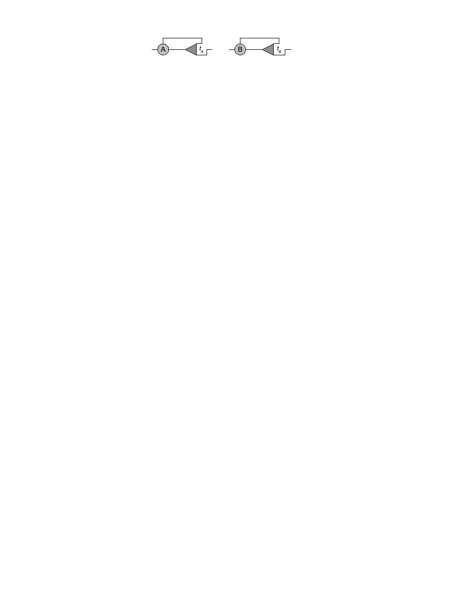
Figure 3: Code before obfuscation
5.4
Obfuscation methods - Structural obfuscation
The obfuscation methods we described up to now were targeted, that is that they modify the code
in some specific locations, they add new code, make the existing code more obscure, but they
always remain focused on a specific part of the program. The approach described in this section
consists in an obfuscation of larger pieces of code by a modification of the code’s structure. The
execution’s main steps will still be executed in the same way since they cannot be modified. We
therefore describe two different approches. The first one tries to make the loop structuration as
obscure as possible. The second one tries to mix the code in such a way that a deobfuscator
cannot detect it but yet the executed code remains unchanged.
5.4.1
Obfuscating loops
In the initial program, loops are usually localized, restricted to a small set of instructions, and
they are either interlocked or succeeding one another. What we would therefore like to achieve
is that the loops stretch on the whole program, without modifying the execution of the program.
To do so, we will work on the graph representation of programs. We will nonetheless reuse
methods that were defined for targeted obfuscation.
We first consider two loops that succeed one another. We would like to create a single non
trivial loop such that a deobfuscator could not tell that this loop is actually made of two distinct
loops that execute independently. Figure 3 gives a representation of a program before applying
obfuscation methods. The two loops are represented by their bodies A and B and their test
conditions t
A
and t
B
.
To obfuscate these loops, we use tests in such a way that their result is as much unpredictable
as possible. We define a variable x that we set to an unpredictable value (using the methods that
were previously described, like using a loop, mathematical results, and others). The obfuscator
must know the current value of x. Thus we use tests that compare the hash value of x to a
constant value: the results of these tests are known before execution, though a deobfuscator will
not be able to tell them.
We now split the loops’ bodies into two parts: A
1
and A
2
, and B
1
and B
2
. Finally we modify
the code structure according to one method of the figure 4.
In the first method, test t selects the currently running loop: it compares the hash value of
x
to a constant value and thus tells whether we are currently executing loop A or B. In the
second method, test t always selects A
2
and test t
′
always selects B
2
. Tests t
A
and t
B
are the
initial tests and were possibly obfuscated using other methods. However, we will have to either
use specific x variables for each such obfuscation or we will have to ensure that the x variable is
not modified during execution of A
1
and A
2
(resp. B
1
and B
2
).
Both methods can be generalized to obfuscate several loops at once: in the first method, you
simply have to replace the t test by a sequence of similar tests (this corresponds to a switch
instruction), and in the second method, the obfuscation should be applied in a circular way (A
1
is connected to A
2
and B
2
, B
1
to B
2
and C
2
, and so on).
This method can actually be applied to other loops, even when they do not succeed one
another.
19
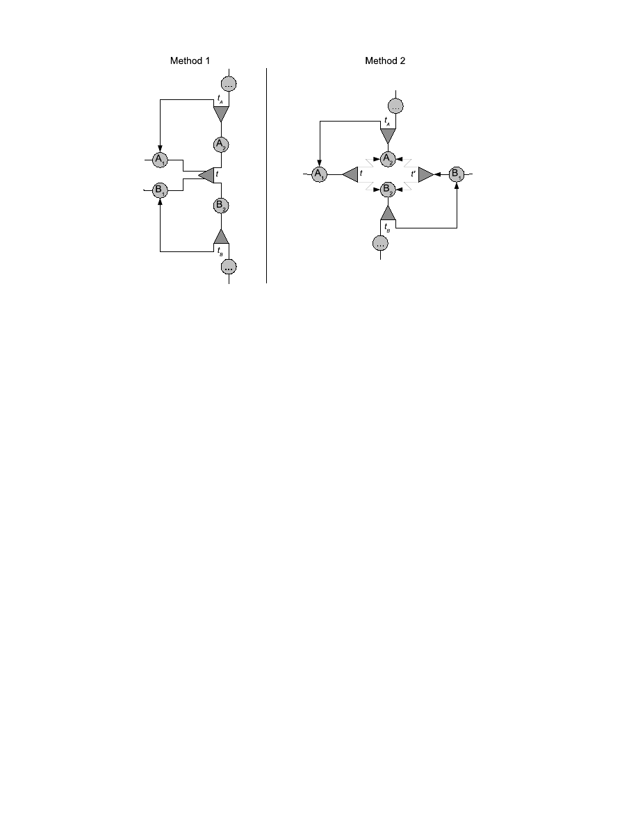
Figure 4: Code after obfuscation
We could also create new fake loops, for instance by taking a piece of code, defining a variable
to a random value and creating the following loop:
int x = 0;
/* Initialize x to a random value (known by the obfuscator). */
for( ; h(x) != A; x++) {
/* A is the hash of the value of x. */
/* Execute the piece of code. */
}
We could also split up SIAs and create fake branches to the new SIAs in order to make the
program’s structure more complex.
5.4.2
Code mixing obfuscation
Code mixing obfuscation aims at jumbling up the code in such a way that, thanks to convenient
jumps, the code is eventually executed as it was at the beginning, but its structure has been
fully modified and is incomprehensible.
We first split the code into several chunks of random size. Then we jumble up these instruc-
tions blocks and we connect them one another using branch instructions. If these branches were
unconditional, then the method would be trivial and the simple representation of the program
as a graph would yield the initial code in a short time.
We therefore use non trivial conditional branches, though all tests will have the same result.
Once again, the methods we described in targeted obfuscation fit our needs. We simply have to
use hardly reductible expressions as well as a counter x whose value changes as the program is
executed and whose hash value is compared in each test to a constant value.
However, a problem remains since the x value must change as the program executes but still
the obfuscator must control it, in particular inside loops. For instance, imagine that we execute
20

the program, increment x and continue the execution. Later, we happen to come back to a block
we already executed, but with a different value of x. Since the test has not been modified, it will
fail and we won’t be able to find the next block to execute.
The solution is to actually number the blocks. s(i) denotes the value by which x is incremented
when we travel from block i to block i + 1. Now suppose that we are currently in block i and
that it contains a branch targetting an instruction in block j
6= i. If j > i, we increment
x
by
P
j
−1
k
=i
s
(k), otherwise we decrement x by
P
i
−1
k
=j
s
(k), before actually travelling through
the branch. This method is all the more interesting as it makes x more unpredictable to a
deobfuscator.
6
Probabilistically implementing τ -obfuscation and code pro-
tection
The main interest in considering τ -obfuscation lies on the fact that code analysts and program
obfuscators/deobfuscators have to face constraints that may greatly differ. To be more precise, let
us consider τ -obfuscation in a viral context. A piece of malware may fulfill its action in an amount
of time that may be definitively unacceptable for an analysis program (namely an antivirus
software). On a practical basis, which user would ever accept his antivirus to monopolize the
computing ressources during hours for analysis purposes
7
. On the contrary a malware can accept
to take a long time to spread or attack. Consequently, τ -obfuscation relies on two challenges:
• to protect the code against analysis: this is the purpose of code obfuscation itself.
• to make the deobfuscation process long enough to prevent, in the case of viruses for instance,
an antivirus (or any other analysis program) to deobfuscate and identify the virus in less
than a given time τ .
The first objective can actually be achieved regardless of the second one. Indeed, in no way do
we require that a virus should take less time than an antivirus to deobfuscate itself. So, rather
than requiring from a virus to work in a very short time, why not imagine a malware that has no
clue as to how it should deobfuscate itself? Then the virus would have to try several methods
in order to do so and it might need two hours to eventually deobfuscate its code. In such a case,
an antivirus would require the same time to deobfuscate the virus. But the main difference lies
in the inability of an antivirus to take such a time to analyse any suspicious file.
Let us mention the fact that Zuo and Zhou [ZZ05] presented new results on time complexity
of computer viruses (virus running time, virus detection procedure). Their main results are:
• For any type of computer viruses, there exists a computer virus v whose infecting procedure
has arbitrarily large time complexity.
• For any type of computer viruses, there is a virus v such that any implementation of v can
have arbitrarily large time complexity in its infection procedure.
Our approach as well as the concept of τ -obfuscation directly relates to their results.
7
Note that the most common protection against malware is “on-access” detection: for instance, before a file
is executed or an e-mail attachment is opened. Though a user would not care whether the antivirus spends one
minute or more to analyze a given document, he would certainly not accept this analysis to delay or differ the
access to any resource (document, e-mail attachment, running an executable...).
21

6.1
A unified approach of code protection
Since obfuscation is only one possible technique that may be used to protect a code against
analysis, let us make our approach more general and extend it to any other code protection
technique: light code armoring
8
, polymorphism, metamorphism... Our goal is to define a unified
perspective for code protection.
Let us consider a set
S of code protection methods (obfuscation, encryption, light code
armoring, polymorphic/metamorphic rewriting techniques...) which may or not be conditioned
by some secret information (e.g a key) to work. Thus, for any s
∈ S and for any program P , s(P )
is a code that cannot be analyzed except with a sufficient amount of time τ . Let us consider now
the set
S
′
of methods which are defined as follows:
∀s ∈ S, ∃s
′
∈ S
′
such that (s
′
◦ s)(P ) ≡ P ,
where
◦ denoted the (non necessarily commutative) functional composition
9
. In other words,
S
′
is the set of deprotection methods with respect to
S. It is important to note that |S| and
|S
′
| may be not equal. Since we consider reversible code protection techniques, we assume that
|S| ≤ |S
′
|. Thus, for some s ∈ S, there may exist S
′′
⊂ S
′
such that
∀s
′′
∈ S
′′
,
(s
′′
◦ s)(P ) ≡ P .
Let us consider the following notation:
S
′
s
=
{s
′
∈ S
′
|(s
′
◦ s)(P ) ≡ P }.
Let us now consider a given malware program P that embeds a code protection routine
C.
This routine chooses at random a method s
∈ S and compute s(P ) which thus is a protected
version of P . This formalism enables to describe many polymorphic techniques as the case where
P
∩ s(P ) = C whereas metamorphism is the case in which we have P ∩ s(P ) = ∅. Whenever the
code s(P ) runs, it deprotects itself by iteratively or randomly applying s
′
∈ S
′
to s(P ).
When considering a given s
∈ S, the deprotection complexity obviously depends on the
probability p
s
′
to find a s
′
∈ S
′
such that (s
′
◦ s)(P ) ≡ P . Then, we have
p
s
′
=
|S
′
s
|
|S
′
|
,
and the search for a deprotection method with respect to a given s
∈ S has complexity O(
1
p
s′
).
Of course, this complexity and the corresponding probability hold under the assumption that
the deprotection methods are uniformly and identically distributed over the set
S
′
.
Since we do not make any additional assumption about the elements in
S, this approach does
not make any difference between light code armoring, polymorphic/metamorphic techniques,
encryption techniques... Protection methods are considered instead. This unified view enables
to focus only on the mathematical properties or structures the sets
S and S
′
should exhibit
rather than on the inherent nature of their respective elements (the protection methods).
From a practical point of view, an easy way of implementing such a method would be to
choose a random protection method among a (possibly infinite) set of methods. To deprotect
a protected code (e.g a virus), one would basically need to successively or randomly test all
inverses of those methods. Let us now describe two implementations of code protection based
on this approach. We will assume that only a (critical) part of the code may be protected. From
a general point of view, the validation of the deprotection can be done in many ways. The most
obvious and easy way to implement this, is to consider a hash function H [Fil05]. Whenever a
deprotection method s
′
is applied to s(S), the value H((s
′
◦ s)(P )) is computed and compared
to a validation data stored somewhere in the code.
8
In this case the purpose is not to forbid code analysis like in [Fil05] but to delay automated code analysis
(e.g. by antivirus).
9
For some particular code protection techniques, we may have (s
′
◦ s)(P ) = P
(e.g. encryption)
22

6.2
Probabilistic encryption
Let us imagine that we want to encrypt some part of the code. If we do not care about the time
we need to decrypt it but if we only require that any analyst (or any analysis software like an
antivirus) cannot decrypt it in less than a given amount of time, then we could choose a random
key of a given entropy n. When needing to decipher the code, we have to test any key of size
n
and so will do the analyst. Except that if the analyst has a great deal of data to process,
this will be unachievable for him at least in a reasonable amount of time. In this general case,
the average complexity is
O(2
n
). It is essential to note that the encryption algorithm must be
carefully chosen so that no attack enables to recover the secret key more efficiently than with an
exhaustive search. A good choice would be to consider a block cipher like GOST [28180]. Since
the entropy key is 256 bits, a number of key bits may be fixed to a constant value in order to
work with shorter keys. Let us stress on a very important point: the aim is not to make the
code unbreakable but to delay any automated cryptanalysis
.
We can achieve probabilistic encryption in several ways, among many others.
6.2.1
A first probabilistic scenario
As a first approach, we can consider choosing a random key for encryption then successively
testing each possible key. If we suppose that testing a key takes one microsecond (10
−6
), then
we will need at most slightly more than one hour to guess a 32-bit key. No antivirus can take
so much a long time to analyze a malware. This solution is not optimal since some constraints
have to be put on the size of the key that cannot have a too large entropy.
So we could also store a random permutation of the chosen key. However, once again, the set
of possible keys would be too large (though this would depend on the presence of similar bits in
the key): by restricting to a specific set of permutations, we can reduce the number of possible
keys. We will discuss this in the upcoming section.
Another solution would be to hide the secret key in the encrypted data. Once the encrypted
data is generated, the key is split into different chunks which are scattered all over the encrypted
data. To do so, we can select random periods for insertion: given a first period p, we insert
those parts every p bytes up to the end, then, given a second period, we continue inserting those
chunks, and so on. Then, when looking for the key, we will have to resolve these periods, by
random guessing. The number of periods is unknown, though it is limited by the size of the key.
Thus, unless it is fixed, we need to know the size of the key before looking for those periods: this
size should be stored in clear. The interest of such a method is to be free of any constraints on
the key itself. Besides, the encrypted code itself is hidden inside the program, since the key is
scattered over it and must be retrieved before being able to extract the encrypted code. The set
of possible periods can also be controlled by controlling the extremes of the random generator.
Yet this method does not conceal perfectly the presence of the virus — though an antivirus
will not be able to identify it. The presence of a great amount of encrypted code in the program
will make the file look suspicious: this gives a clue to an antivirus as to where to look more
specifically for malwares. This issue has been extensively addressed in [Fil06, Chap. 2, 6 and 7]
and a number of solutions have been designed to efficiently fool entropy-based detection.
6.2.2
A more sophisticated approach
In this second approach, the part of the code to protect is encrypted by a public key method. A
private/public key pair (K
pr
, K
pu
) is randomly generated before protecting the code. After that,
the private key K
pr
is discarded. The public key K
pu
is stored inside the deprotection routine.
To deprotect the code, the private key K
pr
has to be guessed by the deprotection routine. For
23

that purpose, instead of trying any possible K
pr
– which would either require a too huge amount
of time or limit the private key size more than desirable – this routine recovers it directly from
K
pu
. Let us consider the following example.
• We consider probabilistic public-key encryption. The main reason to choose this kind of
encryption comes from the fact that it is semantically secure [GM84, MRS88]. In other
words, it represents a polynomially bounded version of perfect secrecy as defined by Shan-
non [Sha49]. Probabilistic encryption is far more secure than its deterministic counterparts
(RSA encryption as an example). It utilizes randomness to reach a provable and strong
level of security. A passive adversary with polynomially bounded computational resources
– this is obviously the case for any automated analysis and detection sofware – cannot
learn anything about the plaintext from the ciphertext. Moreover it is then conceivable
that there exist semantically secure encryption systems where the keys are much shorter
than the message itself. In our case, we will use the Goldwasser-Micali probabilistic en-
cryption [GM84] which is semantically secure assuming the intractability of the quadratic
residuosity problem.
• We will not describe this probabilistic encryption scheme in detail but just describe the key
generation part. Before any code protection step, the protection routine has to generate a
private/public key pair (K
pr
, K
pu
). The general algorithm is:
1. Select two large random, distinct primes p and q, each roughly the same size (by
means of the Miller-Rabin algorithm [MvOV97, p. 146]).
2. Compute n = pq.
3. Select a y
∈ Z
n
such that y is a quadratic non-residue modulo n and the Jacobi symbol
(
y
n
) = 1.
4. The public key K
pu
is the pair (n, y) and the private key K
pr
is (p, q).
• The protection routine then protects the code by probabilistically encrypting it with the
key K
pu
. Then, the pair (p, q) is discarded.
The security of the Goldwasser-Micali probabilistic encryption scheme is based on the quadratic
residuosity problem (QRP ) intractability. QRP is itself as hard as the problem of factoring
integers. Consequently, according to what has been previously considered, the deprotection
routine has to factor the number n. A few efficient algorithms are known to factor integers
[Mor02, Len00], and the best running time is in exp(c log(α).n.(log(log(n))
1−α
)) = L
n
[α, c] where
α
and c are some constants (for the best methods α =
1
3
and 1.5 < c < 2). However, most of these
efficient methods require a huge amount of memory, far more than any commercial antivirus may
consider. Moreover, some mathematical and implementation constraints must be considered in
order to achieve an optimal running time. That is why, for code deprotection purposes, most of
these methods cannot be considered. The best trade-off can be obtained with the quadratic sieve
(QS) methods [Pom84]. Let us note L
n
[α] = exp(
√
log n log log n)
α
+O(1)
. Then, the QS running
time complexity when factoring an integer n is L
n
[1] and the memory complexity is L
n
[
1
2
]. Thus,
the choice of the public key K
pu
has a direct impact on the deprotection method. Simulations
have shown that a 50-digit key could be factored in nearly 30 minutes requiring less than 100
Kb of memory.
Remark 1
.- Public key encryption can also be used to encrypt a symmetric secret key K only
(in other words, a session key as in PGP encryption sofware). Referring to Section 6.2.1, the
interest lies in the fact that the encrypted key E
K
pu
(K) hides the exact entropy of K.
24

6.3
Data transformation
Let us consider that we have at our disposal a set of methods that perform a transformation
of the virus data (incl. code or raw data). Obfuscating the code would mean applying one of
these transformations to the virus data, whereas deobfuscating it would mean finding the inverse
transformation. Let
S be this set of transformations. Among several approaches, let us consider
that
S has a group structure with regard to the law of composition. Then for any transformation
π
∈ S, its inverse π
−1
is also in
S, as well as any composition of transformations of S.
The symmetric group σ
n
– the group of permutations of [1..n] – is a convenient example
for this set of transformations. The main interest in considering data transformation by code
permutation lies in the fact that encrypted content has a very specific statistical profile whereas
permuted data have not. While a detection software will trigger an alarm whenever the code is
encrypted
10
, it will not if the code is only a permutation of itself.
Obfuscating the virus data would be achieved by permuting the bytes of these data. We will
have to consider a cyclic subgroup G of σ
n
, in order to restrict its size (
|σ
n
| = n!). This group has
several interesting properties. In particular, for a given transformation π
∈ σ
n
, its inverse is π
k
,
for a k
∈ [1..n]. Thus the protection routine just picks up a permutation π at random whereas
the deprotection procedure picks up a random permutation π
′
and exhaustively searches for the
right k
′
such that (π
′
)
k
′
◦ π = Id. In this general setting, since the deprotection complexity is
O(|G|), we have to choose a large value of n in order to make the deprotection time long enough.
From a practical point of view, the permutation π may be chosen as the generator of a cyclic
subgroup of σ
n
. Finding the inverse permutation is consequently easy to implement by means of
a simple loop which ranges from 1 to the order of the subgroup. Moreover, the subgroup order
will be chosen as a prime number in order to maximize the number of subgroup generators.
In the previous case, since any permutation has a unique inverse, the set
S
′
is a singleton.
But we may desire for a given code protection method s
∈ S to have |S
′
s
| > 1. This would offer
more flexibility in implementing code protection/deprotection. One solution – among others – is
to consider a fixed ordered set
F of (possibly non-contiguous) bytes {b
i
1
, b
i
2
, . . . , b
i
k
} and a set
of code locations
{i
1
, i
2
, . . . , i
k
}. Whenever deprotection of a program P yields
∀i ∈ {i
1
, i
2
, . . . , i
k
}, P[i] = b
i
,
then the code is considered as deprotected
11
. In this case, the set
F describes the critical part
of the code that must be permanently protected (by randomly permuting it) while the other
(permuted) part of the code may be dummy bytes or dead code. Let us consider the following
permutation of a 9-byte program: π = (384729156). If
F contains the original bytes of the
program whose location indices are
{2, 5, 8} then S
′
=
{π
3
, π
6
, π
9
}.
From a general point of view, it is possible to partition the code into k sets. We choose
k
− j sets to describe the critical part of the code to protect while the j remaining sets are
the non critical part of the code or are dummy/dead code. We then consider k different cyclic
permutation groups, each of them acting over one of the k sets. This latter approach enables
to consider permutation subgroups of far larger size. Indeed, the order of a cyclic subgroup has
the same magnitude as the permutation length. In other words, when considering a single cyclic
permutation group of order n, any antivirus will have to try at most
O(n) permutations to find
its inverse. On the contrary, when considering k different cyclic subgroups, each of them of order
n
i
,
i
= 0, . . . , k
− 1, the complexity rise to O(lcm(n
0
, n
2
, . . . , n
k
−1
) with a maximal value if the
different n
i
are coprime. Of course, an efficient implementation will consider both random value
10
Some Internet providers do not deliver e-mail which contains encrypted attachement, as an example.
11
Let us recall that the validation would of course not compare the raw data but for instance, test the value of
its hash.
25

of k and random (coprime) n
i
. Moreover, in order to forbid the analyst to guess what is the
critical portion really is, and thus to restrict the search of the inverse permutation to this critical
part, an efficient implementation of this protection scheme will prevent this in the following way:
the protected, critical part – let us denote σ(
C) – contains the length over which to apply the
validation hash. If the inverse permutation is not correct, then (σ
′
◦ σ)(C) will contain a random
value of this length thus fooling the analyst: this length may be larger or shorter than the exact
required length, thus any restriction with regards to the inverse permutation length is impossible.
7
Conclusion
In this paper, we have studied how to practically obfuscate executable code. Following Barak
& al results [BGI
+
01], we have proved that with a slightly different formalism, obfuscation still
does not exist. But if any obfuscated code is bound to be successfully analyzed by a human
operator, automated programs (e.g. antivirus software or Intrusion Detection Systems (IDS))
with constant (
O(1)) bounded resources are bound to fail. This is the main perspective of our
work. It is thus conceivable that efficient practical obfuscation techniques will put check on any
detection software in the future, if not already the case.
The practical obfuscation techniques we have presented in Section 5 and 6 have been essen-
tially considered in the case of malware context and under some very particular conditions. But
code obfuscation techniques may have a huge number of positive applications (e.g. copyright
enforcement, digital right management...). The authors are considering as an open problem
whether these techniques may be used for such applications.
References
[28180]
GOST 28147-89. Cryptographic protection for data processing systems, 1980. White
paper, available from http://www.cisco.com/warp/public/732/netflow.
[BGI
+
01] B. Barak, O. Goldreich, R. Impagliazzo, S. Rudich, A. Sahai, S. Vadhan, and K. Yang.
On the (im)possibility of obfuscating programs. In Proceedings of CRYPTO, pages 1
– 18, November 2001.
[CTL97]
C. Collberg, C. Thomborson, and D. Low. A taxonomy of obfuscating transfor-
mations. Technical Report 148, Department of Computer Science, University of
Auckland, July 1997.
[Fil05]
E. Filiol. Strong cryptography armoured computer viruses forbidding code analysis:
the bradley virus. In V. Broucek ed., Proceedings of the 14th EICAR Conference,
pages 201 – 217, May 2005.
[Fil06]
E. Filiol. Techniques virales avancées. Springer Verlag France, 2006. An English
translation is pending and will be in print at the beginning of 2007.
[GM84]
S. Goldwasser and S. Micali. Probabilistic encryption. Journal of Computer and
Systems Sciences
, 28:270 – 299, 1984.
[Kle38]
S. C. Kleene. On notation for ordinal numbers. Journal of Symbolic Logic, 3(4):150
– 155, December 1938.
[Len00]
A. K. Lenstra. Integer factoring. Designs, Codes and Cryptography, 19:101 – 128,
2000.
26

[Mor02]
F. Morain. Thirty years of integer factorization. In F. Chyzak ed., Proceedings of the
Algorithms Seminar 2000 - 2001
, pages 77 – 80, April 2002.
[MRS88]
S. Micali, C. Rackoff, and B. Sloan. The notion of security for probabilistic cryp-
tosystems. SIAM Journal in Computing, 17:412 – 426, 1988.
[MvOV97] A. J. Menezes, P. C. van Oorschot, and S. A. Vanstone. Handbook of Applied Cryp-
tography
. CRC Press, 1997.
[Pap95]
C. Papadimitriou. Complexity Theory. Addison Wesley, 1995.
[Pom84]
C. Pomerance. The quadratic sieve factoring algorithm. In T. Beth and N. Cot and
I. Ingemarsson eds, Advances in Cryptology - Eurocrypt’84
, volume LNCS 209, pages
169 – 182. Springer Verlag, May 1984.
[Sha49]
C. E. Shannon. Communication theory of secrecy systems. Bell System Technical
Journal
, 28:656 – 715, 1949.
[ZZ05]
Z. Zuo and M. Zhou. On the time complexity of computer viruses. IEEE Transactions
in Information Theory
, 51(8):2962 – 2966, 2005.
27
Wyszukiwarka
Podobne podstrony:
Petkov ON THE POSSIBILITY OF A PROPULSION DRIVE CREATION THROUGH A LOCAL MANIPULATION OF SPACETIME
On the Possibility of Speculation under Rational Expectations
The possibility of any?onomy is limited
Military Regulations on the Acceptance of Alternate Religious Practices
Bondeson; Aristotle on Responsibility for Ones Character and the Possibility of Character Change
THE VACCINATION POLICY AND THE CODE OF PRACTICE OF THE JOINT COMMITTEE ON VACCINATION AND IMMUNISATI
Interruption of the blood supply of femoral head an experimental study on the pathogenesis of Legg C
Ogden T A new reading on the origins of object relations (2002)
Newell, Shanks On the Role of Recognition in Decision Making
On The Manipulation of Money and Credit
Dispute settlement understanding on the use of BOTO
Fly On The Wings Of Love
31 411 423 Effect of EAF and ESR Technologies on the Yield of Alloying Elements
Crowley A Lecture on the Philosophy of Magick
On the Atrophy of Moral Reasoni Nieznany
Effect of magnetic field on the performance of new refrigerant mixtures
94 1363 1372 On the Application of Hot Work Tool Steels for Mandrel Bars
więcej podobnych podstron