Full Length Article

Biomass modelling: Estimating thermodynamic properties from the
elemental composition

, Guillaume Boissonnet

, François Maréchal

École Polytechnique Fédérale de Lausanne, Industrial Process and Energy Systems Engineering, Rue de l’Industrie 17, Case Postale 440, CH-1951 Sion, Switzerland

CEA – Grenoble DRT/LITEN/DTBH/Laboratoire des Technologies Biomasse, 17 rue des Martyrs, 38054 GRENOBLE cedex 9, France

h i g h l i g h t s

Accuracy of heating value correlations on a consistent database of biomass samples.

Complete and coherent lignocellulosic biomass model for numerical simulations.

Enthalpy and Gibbs free energy as linear correlations of the elemental composition.

Exergy in terms of thermodynamic properties and composition of the environment.

a r t i c l e

i n f o

Article history:
Received 14 September 2015
Received in revised form 14 April 2016
Accepted 21 April 2016
Available online 3 May 2016

Keywords:
Biomass
Heating value
Modelling
Exergy
Gibbs free energy

a b s t r a c t

In the context of modelling biomass conversion processes, the accurate representation of biomass, which
is a complex and highly variable material, is of crucial importance. This study provides a rather simple
and flexible way to represent biomass, especially suited in the context of thermochemical conversion
processes. The procedure to represent the enthalpy of formation, the Gibbs free energy and the exergy of
biomass in terms of its elemental composition (C, H, O, N, S) and moisture content is outlined.

The correlations relating the heating value to the elemental composition of biomass are evaluated

through a database of over one hundred raw and pretreated biomass samples. Results show that such
correlations can predict the higher heating value (HHV) within an accuracy of 1.93% and 2.38%. One of
the correlations is then applied to represent the enthalpy of formation of biomass as a linear function
of the elemental composition.

The procedure is extended to estimate the Gibbs free energy of formation and subsequently the exergy of

biomass, which are expressed as linear functions of the elemental composition. The method proposed for
the estimate of exergy allows taking directly into account the composition of the reference environment.
Results show that the method proposed in this study agrees within 1% accuracy with the widely used cor-
relation proposed by Szargut et al. (1988). The values obtained for Exergy, over the range of compositions
of the samples considered, vary in general between 105% and 115% of the lower heating value (LHV) and
103% and 107% of the higher heating value obtained using the literature correlation by Boie (1953).

On the basis of these correlations, this study provides the thermodynamic properties of C, H, O, N, S and

bound water ‘pseudo-compounds’ that can be used in the thermodynamic properties evaluation packages
used in flowsheeting software and in numerical simulations for a coherent description of biomass as a
function of its composition.

1. Introduction

The first challenge in the thermochemical modelling of biomass

conversion systems is to model biomass itself, the raw material.
Biomass is not a standard compound and its chemical, elemental
composition, as well as its thermal properties vary significantly.

Different solutions are adopted or suggested, for example, to

model biomass in flowsheeting software. In an example bioethanol
production unit, modelled in ProSim Plus

[1]

, biomass is repre-

sented as a mixture of its chemical constituents by adapting the
properties of glucose, such as the chemical formula, the heat of
formation and the molecular weight, to represent cellulose, hemi-
cellulose and lignin. Aspen Plus

allows the implementation of

organic substances as non-conventional solid compounds through
the definition of attributes in terms of ultimate (i.e. elemental

http://dx.doi.org/10.1016/j.fuel.2016.04.111

0016-2361/

⇑

Corresponding author.
E-mail address:

emanuela.peduzzi@epfl.ch

(E. Peduzzi).

Fuel 181 (2016) 207–217

Contents lists available at

ScienceDirect

Fuel

j o u r n a l h o m e p a g e : w w w . e l s e v i e r . c o m / l o c a t e / f u e l

composition) and proximate (i.e. fixed carbon, volatile matter and
ash content) analysis. The heating value, the heat of formation and
the heat capacity are then calculated by selecting the relevant liter-
ature correlations, generally developed for coal, in the General Coal
Enthalpy Model (HCOALGEN property model

[2]

). The attributes can

be changed through the use of subroutines to represent changes in
composition during conversion, for example during coal devolatili-
sation. Rönsch and Wagner

[3]

analysed the application of the

empiric correlations used in AspenPlus

to model wood and straw.

They showed that the heating value correlations, developed for coal,
generally underestimate the values for biomass and they indicated
which correlations can predict the heating values of average wood
and wheat straw samples within their standard deviation.

The objective of this study is to propose an accurate and consis-

tent definition of biomass, especially relevant for the simulation of
thermochemical conversion processes. The goal is to develop a gen-
eric representation of the thermodynamic properties of biomass
that allows to easily update process performances as a function of
the type of biomass, which is considered on the basis of its elemen-
tal composition. The model developed is general and may be used in
any numerical simulation but in this study it is applied to represent
biomass in the flowsheeting software Vali

by Belsim

[4]

. Therefore

the methodology presented refers rigorously to thermodynamics
but the formalism refers sometimes to this software. Thermody-
namic properties packages offered in flowsheeting software, such
as Vali

, allow in fact the definition of new pseudo-compounds,

that is, user-defined compounds used to model substances that
are not present in the internal database for which thermodynamic
properties need to be defined. In this study, special attention is
given to the coherence of the heating value calculated from the
thermochemical properties of the pseudo-compounds. The heating
value represents the energy content of biomass and is one of the
most important properties for the design and simulation of biomass
thermochemical conversion systems

[5]

The steps leading to the representation of biomass are presented

in detail. First of all a ‘biomass database’, obtained in the context of
previous work, is used to extract information regarding the
elemental composition and heating value of many representative

lignocellulosic biomass samples. This information is used as a basis
for comparing several correlations available in the literature relat-
ing the elemental composition to the heating value in the range
of compositions of biomass types considered in this study. The sys-
tematic comparison of the correlations and corresponding errors
allows one to identify the correlation best fitting the experimental
data. Finally, given a correlation, the approach and the fundamental
assumptions used to model biomass are presented. The properties
considered are the heating value with the corresponding enthalpy
of formation, the heat capacity, the heat of adsorption of the mois-
ture content. Furthermore the modelling approach is extended to
the entropy, the Gibbs free energy and the exergy of biomass. In par-
ticular, the exergy model presented allows the explicit definition of
the exergy of biomass based on its thermodynamic properties and
the properties of the reference environment.

2. The definition of biomass

From a legal standpoint biomass is ‘‘the biodegradable fraction of

products, waste and residues from biological origin from agriculture
(including vegetal and animal substances), forestry and related indus-
tries including fisheries and aquaculture, as well as the biodegradable
fraction of industrial and municipal waste”

[6]

. Biomass therefore

includes a large variety of materials. In this study biomass refers
only to lignocellulosic materials from forestry and agricultural
products, namely wood and straw of different types. Biomass is gen-
erally defined by considering its chemical/structural (i.e. cellulose,
hemicellulose, lignin and extractives), proximate and ultimate anal-
ysis. The ultimate analysis and the heating value are especially
important for the definition of biomass in a thermochemical model,
as they provide the basis for the atomic and energy balance of a con-
version process.

In terms of ultimate analysis, biomass is mainly composed of

C, H, and O, which define, for the most part, its heating value. It also
contains small quantities of N, S, Cl. These six elements make up
the organic phase of biomass. The inorganic phase contains Si, Al,
Ti, Fe, Ca, Mg, Na, K, S, P, and other minor elements which are

Nomenclature

Acronyms
ar

as received basis

daf

dry ash free basis

dry basis

EMC

equilibrium moisture content

fsp

fiber saturation point

HHV

higher heating value

hard wood

LHV

lower heating value

MAE

mean absolute error

MBE

mean bias error

moisture content

RMSE

root mean square error

supplementary information

SRC

short rotation coppice

SRF

short rotation forestry

soft wood

Roman letters
B00

biomass on a dry basis, 0% moisture (–)

standard chemical exergy (kJ mol

)

biomass on a wet basis, X% moisture (–)

;dry

heat capacity, dry basis (kJ kg

B00

)

;wet

heat capacity, wet basis (kJ kg

tot

)

standard Gibbs free energy (kJ mol

)

standard enthalpy (kJ mol

)

HHV

higher heating value (kJ kg

B00

or kJ mol

)

constant by Battley (–)

LHV

lower heating value (kJ kg

B00

or kJ mol

)

molar mass (g mol

)

moisture content referring to bound water (kg

B00

)

fsp

moisture content after evaporation of free water
(kg

B00

)

moisture content (kg

B00

)

ideal gas constant (J mol

standard entropy (kJ mol

)

temperature (K or

°C)

T00

Torrefied biomass, 0% moisture (–)

Greek letters

humidity (kg

tot

)

standard deviation (–)

208

E. Peduzzi et al. / Fuel 181 (2016) 207–217

important for ash characterisation. Biomass usually also contains
traces of heavy metals

[7]

The heating value of a fuel, such as biomass, represents its

energy content. It is defined as the heat released by the complete
combustion of a unit of volume of the fuel at 1 bar (101325 Pa),
considering reactants and products at the same reference temper-
ature

[8]

. The reference temperature, by convention, is considered

here at 25

°C (T

is 298.15 K). It is possible to distinguish between

two types of heating values: the higher heating value (HHV) if the
heat of condensation of water generated in the combustion (from
the hydrogen originally present in the biomass) is recovered and
the lower heating value (LHV) if this water is considered in its
vapour state (and therefore its heat of condensation is not
recovered). Due to the presence of water and ash in biomass, the
HHV and LHV may be referred to on a weight basis: dry basis
(db), dry ash free basis (daf ), or as received basis (ar).

The relationship between HHV and LHV on a dry basis and the

relationship between LHV on a dry basis and LHV on an as received
basis are reported in Eqs.

(1) and (2)

respectively.

HHV

LHV

100

ðkJ kg

ð1Þ

LHV

ð1

ðkJ kg

ð2Þ

and M

are the molar masses of water and hydrogen, H

is the hydrogen mass percentage in the fuel,

is the enthalpy

of vaporisation of water at the reference temperature (in kJ kg

is the humidity (in kg

1
tot

) and

is used to refer to properties

on a mass basis. In this study, unless otherwise specified, all values
refer to dry or dry ash free basis. The evaluation of the ultimate
analysis and the heating value of different biomass types is sum-
marised hereafter with the introduction of the biomass database
used in this study.

3. Biomass database

The ‘biomass database’ used in this study is a collection of

experimental elemental compositions and corresponding HHV
and LHV. These values are obtained, in the context of previous
studies, from the analysis of over one hundred samples, which
include both raw and torrefied biomass. The raw biomass database
relies on the characterisation, carried out by Dupont et al.

[9]

, of 92

representative samples. The standards used to obtain the ultimate
analysis and the heating values are summarised in

Table A.1 in the

supplementary information (SI)

Hereafter, as in the previous study by Dupont et al.

[9]

, the data

is classified in biomass families. Hardwoods (angiosperms) are rep-
resented by broad-leafed trees such as oaks, beech trees, hornbeam
and lime (basswoods) trees. Softwoods (gymnosperms) are
represented by conifers such as pine trees, fir trees, and spruce.
The database includes also short rotation coppice (SRC) and short
rotation forestry (SRF) represented by willow and poplar, and
agricultural biomass represented by straw from barley, corn, rape,
and wheat, and energy crops from alfalfa, miscanthus, fiber and
sweet sorghum, switchgrass, tall fescue, and triticale. The data rel-
ative to torrefied biomass was obtained by Marty

[10]

, by Nocquet

et al.

[11,12]

and other previous studies. The database was further

enriched including biomass chars and, as a reference, coal, from
Parikh et al.

[13]

. The average values of the ultimate analysis and

heating values obtained for the different raw biomass species are
summarised in

Table 1

Results presented in

Table 1

show that biomass composition is

similar across biomass types. However, agricultural residues and
energy crops, display a sensibly smaller heating value and carbon
content and higher ash content than other raw biomass types.

4. Correlations estimating the heating value

The direct measure of the heating value of biomass, through

bomb calorimetry, is a complicated and time-consuming proce-
dure. It can therefore be interesting to use a correlation to calculate
the heating value from other conventional properties of biomass,
i.e. proximate and ultimate analysis, which can be obtained rela-
tively easily and cheaply

[5]

. An extensive review of correlations

relating the heating value of biomass to its ultimate, proximate,
and chemical/structural analysis, with attention to biomass type,
is presented by Vergas-Moreno et al.

[7]

. This review also high-

lights the lack of information which is sometimes encountered in
the literature in terms of the data used to develop and validate
the correlations and their basis (dry basis or dry ash free), but also
in terms of the transcription errors when correlations are referred
to by other authors.

The first model developed to calculate the heating value from

an elemental composition was proposed by Dulong in 1880 and
concerned coal samples. During the 20th century many models
were developed to estimate the heating value of coal and, over
the last 30 years, also of biomass

[7]

. A survey of published corre-

lations is also reported by Channiwala and Parikh

[14]

, who

reviewed several correlation types and relative basic assumptions.
Sheng and Azevedo

[5]

tested the performance of correlations

relating the heating value to the elemental, proximate and chemi-
cal analysis on a large database of biomass samples collected from
the literature. They show that the correlations relating the proxi-
mate composition and the heating value display low accuracy,
but they have recently gained importance among engineers and
researchers due to the ease and speed of proximate analysis

[7]

The correlations based on chemical/structural analysis also present
low accuracy because of the variation of biomass components
properties and chemical composition. On the contrary, the correla-
tions relying on the ultimate analysis are the ones that provide the
most accurate results

[5]

In thermochemical process modelling the use of correlations

relating the heating value to the elemental composition is a good
compromise between accuracy and ease of computation. Given
the database presented in Section

it is possible to either develop

a new correlation or use the ‘biomass database’ to validate the cor-
relations proposed in other studies. The interest in using this data-
base lies in the use of samples which cover a wide range of biomass
fuels, from agricultural to woody and torrefied biomass, and in the
consistency of the measurement procedures. However, given the
relatively small composition variations of the biomass samples,
the unequal distribution across the heating values and in the
interest of a most general approach, correlations from the litera-
ture are validated using the database.

4.1. Evaluation of literature correlations

A survey of correlations from the literature estimating the

heating value from the elemental composition is reported in

Table 2

. These correlations have been developed considering bio-

mass samples or, even if they were developed for coals or other
hydrocarbon fuels, are sometimes used in the context of biomass.

The oldest correlations reported, for reference, were developed

for coal and are the ones by Dulong, Eq.

(3)

, and by Mott, Eq.

(4)

[15]

. The correlation by Boie

[16]

, Eq.

(5)

, was derived using

hydrocarbon fuels with an expected error within 1.8%

[14]

. This

correlation is sometimes used to model biomass in flowsheeting
software

[17–19]

. The relationship proposed by the Institute of

Gas Technology (IGT)

[20]

, Eq.

(6)

, is very general and was

developed on the basis of over 700 coal samples, with an error that
lies within 1.2%

[14]

E. Peduzzi et al. / Fuel 181 (2016) 207–217

209

In the context of biomass, Tillman

[21]

developed a correlation,

Eq.

(7)

, to calculate the heating value of wood and wood barks from

their carbon content and later modified it to extend its validity to
the whole range of biomass materials. Predictions for this equation
are reported to be within 5% error. Eq.

(8)

represents the

correlation developed by Grabosky and Bain offering predictions
claimed to be within 1.5%

[14]

. Channiwala and Parikh

[14]

developed a generalised and unified correlation, Eq.

(9)

, aiming

at simultaneously describing the heating value of solid, gaseous
and

liquid

fuels

within

the

range

% 6 C 6 92:25%,

:43% 6 H 6 25:15%, 0:00% 6 O 6 50:00%, 0:00% 6 N 6 5:60%,

:00% 6 S 6 94:08%, 0:00% 6 A 6 71:4%, 4.745 MJ kg

6 HHV

6 55.345 MJ kg

, where C, H, O, N, S and A represent carbon,

hydrogen, oxygen, nitrogen, sulphur and ash contents of a fuel,
respectively, in wt% (dry basis).

These fuels include terrestrial

and aquatic biomass material, industrial waste and municipal solid
waste, refuse and sludge, as well as chars, coals and coke

[14]

According to the authors this correlation yields a mean absolute per-
centage error of 1.45% and mean bias error (MBE) error of 0.00%.

Sheng and Azevedo

[5]

proposed a new correlation, Eq.

(10)

based on a database of biomass samples collected from the open
literature. According to the authors this relationship provides
90% of predictions within ±5% error.

More recently, Friedl et al.

[22]

used 122 plant biomass samples

and obtained a correlation, Eq.

(11)

, by ordinary least squares

regression (OLS) and by partial least squares regression (PLS)
which allows HHV prediction with a standard error of 2%.

The correlations reported in

Table 2

present different

coefficients and therefore yield different results for the same

composition. Comparing these correlations is difficult because
the authors report different accuracies based on different samples
and composition ranges. Therefore, a comparison of the average
results obtained using these correlations to estimate the HHV of
the raw samples belonging to the ‘biomass database’ considered
in this study is carried out and reported in

Fig. 1

. Most of the cor-

relations accurately reproduce the average HHV of the biomass
samples.

Table 1
Average composition and HHV of different types of biomass on a dry basis. The number of samples of each biomass type is presented in parenthesis.

Hardwood (33)

Softwood (16)

Mix (3)

SRC & SRF (11)

Ag. Biomass (23)

Av.

Carbon (wt%)

49.7

1.0

51.2

1.3

50.8

1.0

49.1

0.3

46.8

1.4

Hydrogen (wt%)

5.8

0.1

5.9

0.2

5.9

0.1

6.0

0.1

5.8

0.2

Oxygen

(%wt)

42.7

1.1

41.9

1.3

40.8

1.3

41.9

1.1

42.3

2.4

Nitrogen (wt%)

0.2

0.1

0.2

0.0

0.3

0.2

0.8

0.5

Sulfur (mg kg

)

171.2

133.7

270.9

443.8

243.3

108.7

609.3

673.8

1,355.5

645.1

Ash, 550

°C (wt%)

1.74

0.64

0.99

0.65

2.33

1.31

2.88

1.08

5.14

2.08

HHV

(kJ kg

)

19811

448.4

20331

704.3

19947

480.9

19552

612.6

18458

703.8

LHV

(kJ kg

)

18612

442.5

19128

707.2

18740

477.5

18321

614.4

17263

703.2

Mix refers to hardwood and softwood samples.

Oxygen is calculated by difference.

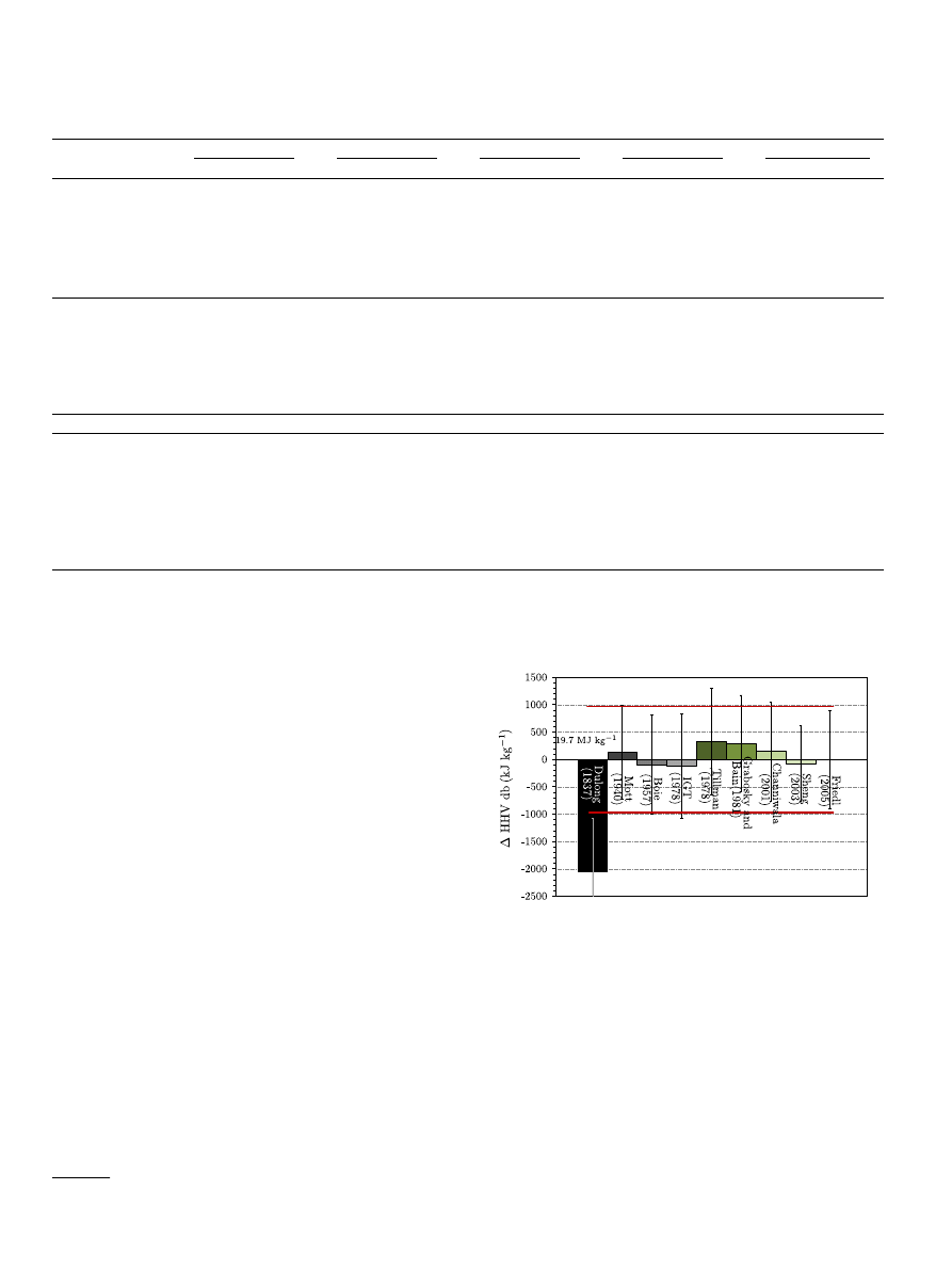
Fig. 1. Evaluation of the performance of literature correlations estimating the HHV
with respect to the measured values of the ‘biomass database’ considered in this
study. The bars represent the difference between the average HHV calculated using
the different correlations and the average HHV measured. The average measured
value is 19.7 MJ kg

. The grey bars represent correlations originally developed for

coal and hydrocarbons whereas the green bars represent correlations originally
developed for or including biomass. The red lines represent the standard deviation
of the measured HHV, the error bars represent the standard deviations obtained
using the correlations. (For interpretation of the references to colour in this figure
legend, the reader is referred to the web version of this article.)

Table 2
Survey of correlations estimating the HHV from the elemental composition

Authors (year)

Correlations: HHV (kJ kg

), dry basis

Dulong (1880)

338

:29 C þ 1442:77 H þ 94:2 S 180:36 O

(3)

Mott-Spponer (1940)

336

:20 C þ 1419:33 H þ 94:2 S ð153:24 72:01 O=ð100 AÞÞ O

(4)

Boie (1953)

[16]

351

:70 C þ 1162:49 H þ 104:67 S 110:95 O þ 62:80 N

(5)

IGT (1973)

[20]

341

:7 C þ 1322:1 H 119:8 ðO þ NÞ 123:2 S=10000 15:3 A

(6)

Tillman (1978)

[21]

437

:3 C 1670:1

(7)

Grabosky and Bain (1981)

328

C þ 1430:6 H þ 92:9 S 23:7 N 40110 ð1 A=100Þ H=C

(8)

Channiwala and Parikh (2002)

[14]

349

:1 C þ 1178:3 H þ 100:5 S 103:4 O 15:1 N 21:1 A

(9)

Sheng and Azevedo (2005)

[5]

1367:5 þ 313:7 C þ 700:9 H 31:8 O

(10)

Friedl et al. (2005)

[22]

:55 C

232 C 2230 H þ 51:2 ðC HÞ þ 131 N þ 20600

(11)

C, H, O, N, S, A represent respectively the carbon, hydrogen, oxygen, nitrogen, sulphur, and ash content expressed in % by mass on a dry basis.

A conversion factor of 2.326 kJ kg

per 1 BTU lb

was considered to adapt the correlation as reported by Mason and Gandhi

[15]

As reported by Channiwala and Parikh

[14]

Here O

is the sum of oxygen and other elements in the organic matter (S, N, Cl, etc.) and is calculated by difference O

= 100

C H A.

As far as the authors know this is the only correlation, considered in this study, for

which a validity range is specified.

210

E. Peduzzi et al. / Fuel 181 (2016) 207–217

The accuracy of the correlations has been evaluated using the

raw and torrefied samples belonging to the representative
‘biomass database’ presented above. Biomass char is considered
separately from the database as its ultimate analysis and heating
values were taken from the literature. The performance has been
evaluated considering the error between experimental and
computed HHV according to the root mean square error RMSE,
mean absolute error (MAE) and MBE as defined in the

. The

MBE represents the bias error of the correlation: a positive value
indicates that the correlation generally overestimates the observed
value. The correlations have also been evaluated considering the
percentage of predictions below 5% error and the coefficient of
determination R

. The values of these parameters for all correla-

tions listed in

Table 2

are listed in

Table 3

for the ‘biomass data-

base’ excluding char on the left and including char on the right.

Excluding char from the ‘biomass database’, the MAE, obtained

using the correlations is in the range of 1.93–2.38% (excluding
Dulong’s correlation). These values are slightly higher than the
reproducibility limit of 1.5% specified by the European Standard
(EN) for the measurement by bomb calorimetry (XP CEN/TS
14918) which shows the high accuracy of the correlations. The best
performing correlations are the most recent ones, Eqs.

(11) and

(10)

by Friedl et al.

[22]

and Sheng and Azevedo

[5]

. However,

considering only biomass and torrefied biomass, the coefficient of
determination is low for all the correlations ranging from 0.54 to
0.64. Including char significantly increases the range of the HHVs
with respect to the scattering of the measurements. This, therefore,
drastically improves this coefficient with values ranging from 0.92
to 0.94. The accuracy remains similar for most correlations with a
significant increase in the RMSE for the correlations by Sheng and
Azevedo

[5]

and Tillman

[21]

The equation that best fits the experimental data available in

this study is the Eq.

(11)

by Friedl et al.

[22]

(Section

4.1

). However,

this correlation features a second order dependency to the compo-
sition which is not compatible with the general approach proposed
in this study that requires a first order polynomial to describe bio-
mass properties as a linear function of its elemental composition.
The correlation retained to model biomass in this study is Eq.

(5)

by Boie

[16]

which is linear with respect to the biomass con-

stituents and presents low MBE. This correlation has been used
in previous studies describing biomass thermochemical conver-
sion, for example, by Gassner and Maéchal

[23]

and Tock et al.

[24]

As shown in

Fig. 2

, Boie’s relationship can represent the HHV

over the range of compositions of the ‘biomass database’ including
torrefied wood and chars, and coal as well as the differences
between biomass types when considering the average values.

5. Biomass thermodynamic properties model

The model presented in this study is general and can be used in

numerical simulations and any flowsheeting software which
allows the definition of new pseudo-compounds to represent sub-
stances not present in the internal database. The pseudo-
compounds chosen here are the most abundant elemental con-
stituents of biomass, which are carbon, hydrogen, oxygen, sulphur,
nitrogen, and bound water. This study provides the thermodynamic
properties to be assigned to these pseudo-compounds to have a
representation of biomass yielding coherent mass and energy
balances.

Using this approach it is possible to model any biomass as a

mixture of these pseudo-compounds provided that partial flows

Table 3
Accuracy of correlations in literature estimating the HHV for the ‘biomass database’ considered in this study.

Excluding char

Including char

RMSE
(kJ kg

)

MAE (%)

MBE (%)

D5% (%)

RMSE
(kJ kg

)

MAE (%)

MBE (%)

D5% (%)

Dulong (1880)

2176

10.51

10.38

4.6

0.54

2148

10.23

10.07

7.9

0.92

Mott-Spooner (1940)

671

2.20

0.76

90.7

0.56

691

2.26

0.58

91.2

0.92

Boie (1953)

[16]

656

2.28

0.42

89.8

0.58

669

2.28

0.37

89.5

0.93

IGT (1978)

[20]

672

2.38

0.56

88.9

0.58

681

2.40

0.62

89.5

0.92

Tillman (1978)

[21]

665

2.43

1.73

89.8

0.68

1185

2.97

2.31

86.0

0.94

Grabosky et al. (1981)

658

2.29

1.56

90.7

0.64

681

2.31

1.33

90.4

0.93

Channiwala and Parikh (2002)

[14]

663

2.20

0.81

91.7

0.58

668

2.19

0.79

91.2

0.93

Sheng and Azevedo (2005)

[5]

611

2.08

0.26

94.4

0.62

989

2.56

0.83

89.5

0.92

Friedl et al. (2005)

[22]

577

1.93

0.06

92.6

0.66

592

1.93

0.04

93.0

0.94

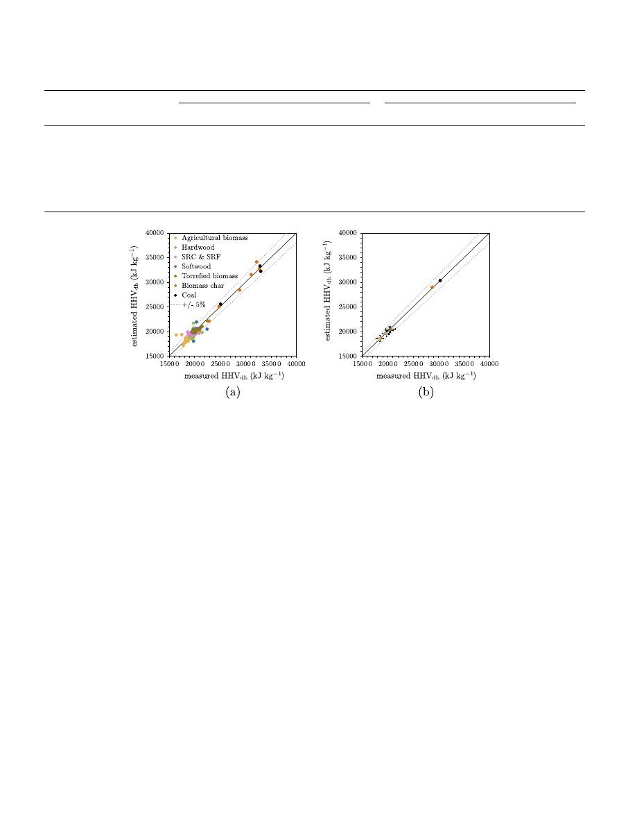
Fig. 2. Use of Boie’s correlation to predict the HHV of different types of biomass, torrefied biomass from the biomass database as well as char and coal: (a) predicted vs
experimental values, (b) average predicted vs average experimental values and relative standard deviation. Error bands of ±5% are displayed.

E. Peduzzi et al. / Fuel 181 (2016) 207–217

211

(or the ultimate composition) is given. The pseudo-compounds are
considered to be solid except for the bound water that will behave
as normal water in the liquid and the gas phase. The thermody-
namic properties of the biomass pseudo-compounds, which are
necessary in flowsheeting tools, are:

The enthalpy of formation of the elemental constituents, to

coherently represent the energy balances of biomass thermo-
chemical transformations.

The heat capacity of the solid, in order to take into account the

sensible heat of biomass.

The enthalpy of formation of bound water (optional), to coher-

ently assess the energy balances during drying processes.

The Gibbs free energy (optional), to define the ‘available energy’,

or ‘exergy’ of biomass.

In this study, the properties of the pseudo-compounds are

defined as being independent of the composition considered. This
feature makes the model very flexible and simple as, once the
properties are implemented, the only information required to rep-
resent biomass is its average elemental composition (and moisture
content) that can be obtained experimentally for a specific biomass
considered.

5.1. The enthalpy of formation

Although biomass is not a pure substance and does not have a

standard value for the enthalpy of formation, it is possible to com-
pute the value of

;BM

from the HHV. Given the combustion reac-

tion stoichiometry, Eq.

(12)

the HHV may be defined as the

additive inverse of the enthalpy of reaction of combustion,

, as

expressed in Eq.

(13)

. Combining Eqs.

(12) and (13)

, and considering

water in its liquid state (H

) it is therefore possible to calculate the

enthalpy of formation of biomass

;BM

þ 1 þ

þ w

ðlÞ

þ CO

þ w SO

ð12Þ

HHV

ðlÞ

;CO

þw

;SO

;BM

1 þ

þ w

ðkJ mol

Þ ð13Þ

When defining the

;BM

, the normalisation used to define bio-

mass composition should always be specified. In this study compo-
sition is referred to 1 mol of carbon. Other studies use 6 mol of
carbon with reference to the structure of glucose. Furthermore, it
should be underlined that a small error on the HHV directly affects
the

;BM

for which it becomes relatively more important (a 5%

error on the HHV can represent a 20% difference on the

;BM

A general linear correlation relating HHV and composition can

be expressed in the form of Eq.

(14)

HHV

¼ eA C þ eB H þ eC O þ eD N þ eE S ðkJ kg

ð14Þ

C, H, O, N and S are the mass percentages of carbon, hydrogen, oxy-
gen, nitrogen and sulphur. For simplicity, these values are here
taken on a dry ash free basis and the corresponding HHV is there-
fore also on the same basis.

The general linear relationship between the higher heating

value of biomass and its composition, Eq.

(14)

, may be re-written

on a molar basis. Considering 1 mol of carbon as reference for
the molar composition of biomass, the molar HHV of biomass

may be expressed by Eq.

(15)

, where x

; y; z and w are expressed

in mol and M

in g mol

HHV

ðCH

Þ ¼ ~A M

þ x ~B M

þ y ~C M

þz ~D M

þ w ~E M

ðkJ mol

ð15Þ

By equating Eqs.

(15) and (13)

, and solving for the

;BM

a lin-

ear correlation is obtained, Eq.

(16)

, relating directly the

;BM

the elemental composition of biomass.

;BM

ðCH

Þ ¼ ~A

;CO

þ x ~B

1
2

ðlÞ

þ y ~C

þ z ~D

þ w ~E

þ x

þ y

þ z

þ w

ðkJ mol

ð16Þ

The coefficients of Eq.

(16)

represent the partial derivatives of

;BM

with respect to the variations in biomass composition,

they can be used to obtain the enthalpies of formation of the
pseudo-compounds that describe biomass.

As shown in Section

, Boie’s HHV relationship may be consid-

ered valid over a wide range of compositions. It is therefore
possible to use the same pseudo-compounds to describe raw and
torrefied biomass. The HHV relationships provide a general way
to describe biomass, which may be acceptable for engineering
applications. The outlined procedure allows to consistently
model the HHV and the enthalpies of formation involved in the
torrefaction and gasification of biomass.

5.2. Gibbs free energy of formation

The Gibbs free energy of formation of biomass can be expressed

in terms of its enthalpy and entropy of formation according to Eq.

(17)

;BM

ðkJ mol

ð17Þ

where

;BM

can be expressed in terms of the absolute entropy S

and the entropy of the atomic constituents of biomass as shown in
Eq.

(18)

;BM

¼ S

atoms

ðJ mol

ð18Þ

Unlike the HHV, from which it is possible to calculate the

;BM

, experimental values of entropy of complex organic mole-

cules are rarely available in the literature. Battley

[25]

proposes a

correlation, Eq.

(19)

, based on the experimental values of entropy

of solid organic substances of biological interest, including cellular
data from previous studies.

¼ ð1 K

atoms

ðJ mol

ð19Þ

is the constant reported by Battley

[25]

with a value of 0.813 and

atoms

are the atomic absolute entropies which can be determined

from the reference substances (carbon, H

, O

, N

, sulphur), avail-

able for example in

[26,27]

and reported in the

SI, Table A.2

In subsequent studies, Battley and Stone

[28]

show that Eq.

(19)

is especially accurate for high molecular weight substances, with
an error of ±1% for substances having a molecular weight higher
than 300 g mol

. Whereas for lower molecular weight substances

the error generally lays within ±3% even though some outliers are

A complete combustion reaction is presumed with all nitrogen completely

transforming to N

during combustion.

and

are omitted as they are equal to zero.

212

E. Peduzzi et al. / Fuel 181 (2016) 207–217

present (at ±30%). Alternatively, the S

of a complex organic mole-

cule can be computed by a group contributions method taking into
account basic structural information and functional groups, as for
example the Joback’s method

[29]

. Nevertheless, given the difficul-

ties in pinning down the exact structures of the main molecular
components of biomass (for example lignin and hemicellulose)
the application of a group contribution method results difficult.
In the context of this study Battley’s method is used to determine
the entropy of biomass, S

, because of the relatively good results

obtained in comparison with Joback’s method for simple organic
molecules and its simplicity. An alternative to Battley’s method is
the correlation proposed by Song et al.

[30]

, linearly relating

entropy to elemental composition, statistically based on the data
of a set of biologically important molecules.

Given the correlation expressing the enthalpy of formation, Eq.

(16)

, and the entropy of formation, Eq.

(19)

, it is possible to express

the Gibbs free energy as shown in Eq.

(20)

;BM

ðCH

Þ ¼

þ T

1000

þ x

þ T

1000

þ y

þ T

1000

þ z

þ T

1000

þ w

þ T

1000

þ x

þ y

þ z

þ w

ðkJ mol

ð20Þ

The Gibbs free energy of formation assigned to the pseudo-

compounds and therefore to biomass can optionally be taken into
consideration in the thermochemical modelling of biomass
conversion.

It should be underlined however that the pseudo-compounds

are ‘artificial’ elements designed to reproduce the properties of
biomass and biomass itself cannot be considered as a substance
at equilibrium. Therefore, the values of Gibbs free energy are not
intended to be used in equilibrium calculation involving Gibbs free
energy minimisation. Nevertheless, these values can be used to
represent the ‘available energy’ or ‘exergy’ value of biomass coher-
ently as it is shown in the next section.

5.3. Exergy of biomass

The exergy concept is often used in the literature to analyse the

performance of thermal and chemical processes. Exergy is defined
as the maximum amount of work that can be obtained by bringing
a system to a state of thermodynamic equilibrium with the
common components of the environment by means of a reversible
process. Examples related to the conversion of biomass are the
analysis by Van Rens et al.

[31]

on biomass to fuel plants, the study

of the role of torrefaction for biomass gasification by Prins et al.

[32]

, the comparison of different types of gasifiers by Gassner

and Maréchal

[33]

and several others.

In these studies the definition of the exergy of biomass relies on

correlations expressing exergy as a function of composition. The
most cited correlations are the ones proposed by Szargut and
Styrylska

[34]

based on regression equations of the exergies of

standard organic substances. Different correlations are proposed
by Kotas

[35]

and Song et al.

[30]

. Other methods based on group

contributions are proposed by Shieh and Fan

[36]

Given the correlations presented in the previous sections of this

study, it is interesting to calculate the exergy of biomass starting

from its thermochemical properties. Taking into consideration
the combustion reaction, expressed in Eq.

(12)

, and the Gibbs free

energy, as shown in Eq.

(20)

, the standard chemical exergy of a fuel

can be expressed by Eq.

(21)

;BM

þ 1 þ

þ w

þ B

;CO

ðlÞ

þ w B

1 þ

þ w

y
2

ðkJ mol

ð21Þ

The standard chemical exergy, B

of the reference species is

related to their concentrations in the environment, considered at
standard temperature and pressure. Two alternative models often
used to represent the standard environment are the ones
developed for example by Szargut et al.

[37]

and Ahrendts

[38]

as reported by Bejan and Tsatsaronis

[39]

For gases belonging to the atmosphere it is possible to calculate

the standard chemical exergy, under the assumption of ideal
gas behaviour, considering their mean partial pressures (or
concentrations), P

, as shown by Eq.

(22)

¼ R T

ðkJ mol

ð22Þ

R is the ideal gas constant equal to 8.314 J mol

, reference

mean partial pressures, P

, are reported in

Table A.3 in the SI

The environment is considered at normal temperature and
pressure: T

= 298.15 K, P

= 101.325 kPa.

It is possible to express the exergy of biomass, again in terms of

a linear correlation of its elemental composition, in the form of
Eq.

(23)

. This equation is obtained given (i) Eq.

(21)

, (ii) the partial

pressures of the reference species in the atmosphere and (iii) the
standard chemical exergies of the reference species in the
environment

;BM

ðCH

Þ ¼

;CO

þ B

;CO

þ x

1
4

1
2

ðlÞ

1
2

ðlÞ

1
4

þ y

1
2

þ z

1
2

þ w

;SO

þ B

;SO

¼ B

þ x B

þ y B

þ z B

þ w B

ðkJ mol

ð23Þ

As for the correlations for the enthalpy of formation and the

Gibbs free energy of formation presented in this study, it is possible
to assign a value of standard chemical exergy to the pseudo-
compounds of biomass to represent its exergy.

5.4. Water content

Biomass, wood in particular, is a hygroscopic material and its

water content is generally expressed in terms moisture content
(MC) (water content on a dry basis).

Water molecules are adsorbed

on biomass surfaces (bound water) up to MC corresponding to the

The standard chemical exergies of the reference species in the environment can

be taken for example from Szargut et al.

[37]

or Ahrendts

[38]

, and reported in the

(Tables A.3 and A.2)

Sometimes the water content is expressed in terms of humidity

(water content

on an as received basis).

E. Peduzzi et al. / Fuel 181 (2016) 207–217

213

fiber saturation point (fsp), which for most wood species falls
between 25% and 30%

[40]

. For higher MC, water exists in cell

cavities and within the pores (free water) and its thermodynamic
properties are essentially the ones of liquid water

[41]

. In this sec-

tion the new pseudo-compound H

bound

is defined in analogy with

the previous sections, in the attempt to represent the thermody-
namic properties of bound water in biomass.

The enthalpy of formation of (bound) water can be described with

respect to the enthalpy of liquid water by the differential heat of sorp-
tion,

sorp

[42]

. As a first approximation the enthalpy of formation

of bound water (H

bound

) can therefore be defined by Eq.

(24)

bound

¼ H

ðlÞ

sorp

ðkJ mol

ð24Þ

where

sorp

is an average value of

sorp

between 0 and the fsp

water content

Stanish et al.

[43]

proposed an approximation assuming

sorp

varies quadratically with the bound water content (M

) and it is

40% of the latent heat of liquid water (

) when the water

content is 0%. This approximation is expressed by Eq.

(25)

sorp

¼ 0:4

fsp

ðkJ mol

ð25Þ

From Eq.

(25)

it is possible to calculate the value of

sorp

. For

example, at 298.15 K (25

°C), neglecting the temperature depen-

dence of

and considering a fsp of 30%,

sorp

is of

6.348 kJ mol

The Gibbs free energy of bound water can be described in terms

of its enthalpy and entropy of formation. The considerations car-
ried out by Dunitz

[44]

in the context of ice, crystalline salts, pro-

teins and bio-molecules, show that the entropy cost of transferring
a water molecule from the liquid state to a surface,

sorp

can vary

the

range

between

and

7 cal mol

and

29.288 J mol

). Considering the entropy cost from liquid

water to ice,

28.95 J mol

as the

sorp

, and the

sorp

esti-

mated before, the

sorp

, with respect to liquid water, at

298.15 K, is 2.272 kJ mol

The Exergy of bound water in biomass can be estimated consider-

ing its formation as a phase change with respect to water in its refer-
ence conditions in the environment, as shown in general by
Hinderink et al.

[45]

. In this case the phase change is from vapour

to liquid,

cond

, and from liquid to bound,

sorp

, which results in

Eq.

(26)

bound

¼ B

;

cond

sorp

ðkJ mol

ð26Þ

Considering again the properties of the reference species in the

environment, taken from

[37]

and reported in

Table A.3 in the SI

and the thermodynamic properties of water, as reported in

[26]

the estimate of B

bound

is 3.19 kJ mol

5.5. Heat capacity

Another property required for the description of the pseudo-

compounds is the heat capacity (c

;dry

). The heat capacity of

biomass is considered independent of its elemental composition
and dependent on its temperature T on the basis of the model pro-
posed by Kollman

[46]

, Eq.

(27)

, which therefore applies to each of

the solid pseudo-compounds considered.

;dry

¼ 0:00486 T 0:21293 ðkJ kg

ð27Þ

The coefficients for heat capacity of the solid are not reported here,
they can be obtained by multiplying the coefficients of Eq.

(27)

the molar mass of each pseudo-compound. Alternatively, other

correlations are available in the literature which are reviewed by
Radmanovic´ et al.

[47]

. These correlations are generally valid in a

temperature range varying between 273 and 373 K. For higher tem-
peratures, between 313 and 513 K, the heat capacity measurements
for 21 biomass types and fast pyrolysis chars, are reported by
Dupont et al.

[48]

To obtain the heat capacity on a wet basis, it is possible to con-

sider the wet biomass as a mixture of dry biomass and water

[49]

as shown in Eq.

(28)

;wet

ðTÞ þ ð1

Þ c

;dry

ðkJ kg

ð28Þ

where c

;water

ðTÞ represents the heat capacity of water at the tem-

perature T.

6. Discussion

6.1. The biomass model

The model presented in this study provides a set of linear corre-

lations relating the enthalpy of formation, the Gibbs free energy and
the exergy of biomass to its composition. The coefficients of these
correlations are summarised in

Table 4

and they can be used to

express the enthalpy of formation, the Gibbs free energy and the
exergy of the pseudo-compounds representing the C, H, O, N, S
and bound water content of biomass. The numerical values are
obtained by taking into consideration Boie’s and Battley’s correla-
tions, thermodynamic properties and standard chemical exergies
(as calculated by Szargut et al.

[37]

) of the reference substances

as reported in

Table A.2 in the SI

The results obtained in terms of

;

, and S

, for several

molecules relevant to biomass are displayed in

SI in Fig. A.4

and

when possible, compared to literature values showing a good
agreement of the proposed correlations.

To complete the biomass model so it can be used, for example,

for a preliminary analysis of a thermochemical conversion process,
it is necessary to fix a reference composition of the inherently vari-
able biomass. For this purpose, and in the absence of experimental
values,

it is possible to use the average value of woody biomass

composition of the ‘biomass database’. Averaging the elemental
composition for hardwood, softwood, SRC and SRF, represented in

Table 1

, and normalising it to a dry ash free basis, yields:

:40

:76

:02

(or equivalently C

:40

:64

:003

corresponding to

mass percentages of 50.81% carbon, 5.96% hydrogen, 43.05% oxygen,
0.18% nitrogen). The average ash content amounts to about 1.3%.

Applying the correlations proposed in this study using the

numerical values of the coefficients as summarised in

Table 4

the properties of the average biomass, C

:40

:64

:003

, are

(normalised

1 mol

carbon):

¼ 120:49 kJ mol

¼ 80:95 kJ mol

, HHV = 442.10 kJ mol

(or 19.959 MJ kg

LHV = 442.29 kJ mol

(or 18.659 MJ kg

) and B

¼ 495:82 kJ mol

(or 20.918 MJ kg

It should be underlined that this study does not take into

account the effect of the ash content and composition and only
attempts to consider the effect of moisture (free water has the same
properties as water). This is because the biomass types taken into
consideration are generally relatively dry and have low ash
content.

6.2. The representation of exergy

This study proposes a model for the representation of the

exergy of biomass based on its thermochemical properties. It is

An overview of the chemical composition of different types of biomass is carried

out by Vassilev et al.

[50]

214

E. Peduzzi et al. / Fuel 181 (2016) 207–217

therefore interesting to compare the results obtained with the
method proposed by Szargut et al.

[37]

and widely used in the

literature.

Eq.

(29)

represents the correlations proposed by Szargut and

Styrylska

[34]

, as reported by Szargut et al.

[37]

, to express the

chemical exergy of a fuel with respect to its LHV as a function of
the elemental composition. Eq.

(30)

concerns wood and Eq.

(31)

concerns bituminous coal, lignite, coke, and peat.

b ¼

LHV

ð29Þ

wood

:0412þ0:2160

0:2499

1þ0:7884

þ0:0450

0:3035

ð30Þ

coal

¼ 1:0437þ0:1896

þ0:0617

þ0:0428

ð31Þ

C, H, N, O are the mass percentages of carbon, hydrogen, oxygen

and nitrogen. The correlations for wood is valid for O/C

6 2.67 with

a mean accuracy of ±1.5% whereas the correlation for coal is valid
for O/C

6 0.667 and ±1%.

These types of correlations are used because biomass, and many

industrial technical fuels such as coal and other hydrocarbons, are
solutions of numerous and often unknown chemical compounds,
for which it is difficult or even impossible to accurately determine
the thermochemical properties.

The comparison between the correlations proposed in this study

and the ones proposed by Szargut and Styrylska

[34]

is carried out

considering the elemental compositions of the sample belonging to
the biomass ‘database’ enriched with biomass char and coal sam-
ples and described in Section

. For the sake of simplicity and for

the comparison carried out in this study all biomass compositions
taken into account are normalised to the dry ash free basis. The
ratios between exergy (Eq.

(23)

) and the heating values as esti-

mated in this study against the ratios obtained considering Szar-
gut’s correlations are displayed in

Fig. 3

. On the right side of this

Figure (a) the heating value is represented by the LHV
(

b ¼ B

=LHV), whereas on the left side (b) the heating value is rep-

resented by the HHV (

¼ B

=HHV). The relationship between LHV

and HHV is reported by Eq.

(1)

. For char and coal samples the exergy

values according to Szargut are calculated with Eq.

(31)

whereas for

all the other samples they are calculated with Eq.

(30)

As mentioned before, the correlations presented in this study are

evaluated considering the composition of the reference environ-
ment as considered by Szargut et el.

[37]

. Results are compared

with the values obtained considering a different set of standard
chemical exergies of the reference species, as for example the one
proposed by Ahrendts

[38]

, which are displayed in grey in

Fig. 3

This comparison shows that the correlation presented in this

study is closely related to the one proposed by Szargut et al.

[37]

Table 4
Summary of the numerical values of the coefficients of the model presented in this study.

Pseudo-compound

(g mol

)

(kJ mol

)

(kJ mol

)

(kJ mol

)

Carbon: C

12.0107

28.89(4308300)

30.28(5661053)

440.545

Hydrogen: H

1.008

25.74(4998820)

9.90(6362655)

108.121

Oxygen: O

15.999

177.51(3343000)

152.65(1032805)

150.664

Nitrogen: N

14.007

87.96(2076000)

111.18(4819990)

111.545

Sulphur: S

32.06

38.76(202000)

46.53(1779781)

593.100

Bound water

: H

bound

18.01528

ðlÞ

6:438

ðlÞ

þ 2:294

3.076

Free water

: H

free

18.01528

ðlÞ

The number of significant figures is limited by the ones of the HHV correlations reported in the literature. However, if these values are intermediate results, all digits

(reported in brackets) should be used to obtain the same values of the initial correlations considered.

The properties

ðlÞ

and

ðlÞ

can be found in thermodynamic properties tables. In this study the values of

285.830 kJ mol

and

237.141 kJ mol

are

used, as reported by Atkins and de Paula

[26]

The properties of free water are equivalent to those of liquid water at standard conditions. The standard chemical exergy of liquid water is taken from

[37]

ðlÞ

¼ 0:9 kJ mol

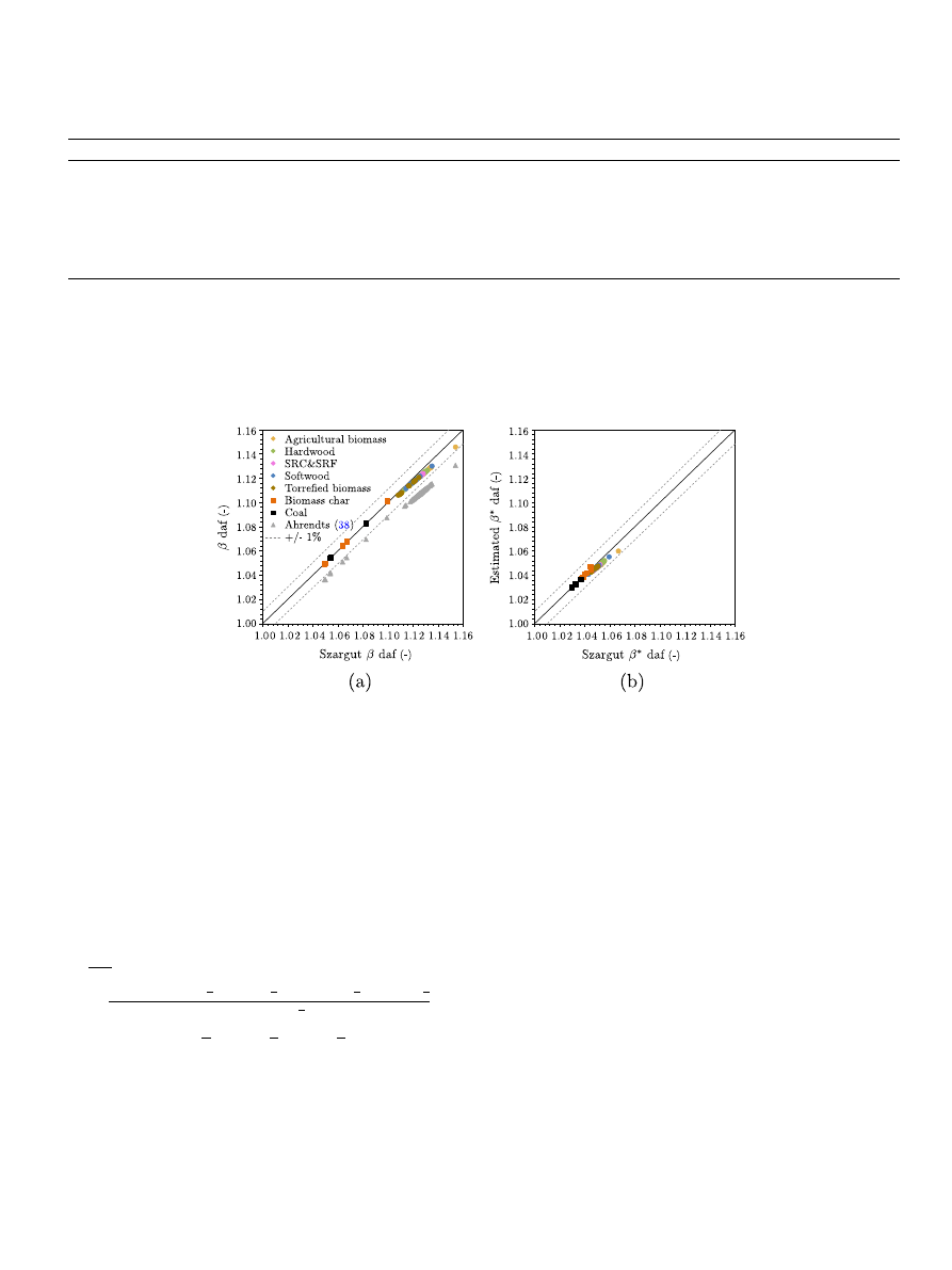
Fig. 3. Ratio between the exergy and the heating value as estimated in this study against the ratios obtained considering the correlations by Szargut et al.

[37]

for wood

(circles) and for coal (squares). The data is relative to different types of biomass, torrefied biomass char and coal. The ratio is reported in (a) with respect to the LHV and in (b)
with respect to the HHV. Grey points represent values obtained considering the reference environment defined by Ahrendts

[38]

, whereas all other values are obtained taking

into consideration the reference environment defined by Szargut et al.

[37]

E. Peduzzi et al. / Fuel 181 (2016) 207–217

215

Results are very similar and, in the range of compositions
considered in this study, lay within ±1% to those obtained using
Eq.

(30)

for dry biomass. This result is expected as the same refer-

ence environment composition has been assumed.

In contrast to previously published correlations,

[37,30,35]

which assume the exergy of biomass to be independent from the
environmental parameters, the approach proposed in this study
can take directly into account the level of components of the envi-
ronment. The results show that the exergy variations are indeed
small.

Furthermore, within the range of compositions considered, the

values of exergy vary between about 105% and 115% of the LHV
whereas they display a smaller variation, between 103% and
107% with respect to the HHV. This justifies the approximation of
the chemical exergy of a fuel with its HHV as it is often observed
in the literature

[39]

7. Conclusions

The biomass model presented in this study allows a coherent

description of the mass and energy balances in the modelling of
biomass thermochemical conversion processes, such as torrefac-
tion, pyrolysis, combustion and gasification. The main contribu-
tions of this study are:

The evaluation of the accuracy of correlations available in the

literature relating biomass elemental composition to its heating
value on a large and consistent database of woody, straw and
torrefied biomass samples.

Given the evaluation of the literature correlations for the HHV, a

flexible and accurate definition of biomass in terms of heat of
formation is proposed.

The method for the estimation of the entropy of complex

organic molecules by Battley

[25]

is extended to biomass.

Gibbs free energy is represented using entropy and enthalpy of

formation correlations.

Exergy is represented given the Gibbs free energy correlation,

which conveniently allows directly taking into consideration
the reference composition of the environment.

A complete and coherent biomass model is presented (sum-

marised in

Table 4

). The model is implemented in the software

Vali

but that could also be used in other calculation procedures.

The approach used in this study is based on the elemental com-

position of biomass and all information relative to structure and
molecular composition is not taken into consideration. Further
study regarding biomass characterisation and the definition of its
properties would be required to fully take into account and estab-
lish the importance of structure with respect to composition, in
terms of enthalpy, entropy, Gibbs free energy and exergy. The
structure information may be useful to model and highlight the
differences between biomass conversion pathways to obtain differ-
ent molecules, for example, in the context of biorefineries. Never-
theless, the elemental composition of biomass can be used to
predict reasonably well the thermodynamic properties of biomass,
most importantly the enthalpy of formation and also give an esti-
mate of its Gibbs free energy of formation and its exergy. Further
investigation is also required to take into better account the effect
of ash and moisture content. It would be interesting in fact to
extend the results and the approach developed in this study to
highly wet and high ash content biomass, as for example animal,
agricultural or food waste. Furthermore the same approach could
be extended to the representation of coal.

The model developed is suitable, given the information

generally available for biomass properties, for the accurate

representation of biomass, and in particular woody biomass, in
the context of the modelling and evaluation of thermochemical
conversion process chains.

Acknowledgements

The research for this paper was in part financially supported by

the Swiss Competence Center for Energy Research BIOSWEET - Bio-
mass for Swiss Energy Future and in part by the Commissariat à
l’énergie atomique et aux énergies alternatives of Grenoble (CEA-
Grenoble) in France. In particular the authors would like to
acknowledge Capucine Dupont (Biomass Technology Laboratory,
CEA-Grenoble) who provided most of the experimental data used
in this study as well as helpful discussion.

Appendix A. Supplementary material

Supplementary data associated with this article can be found, in

the online version, at

http://dx.doi.org/10.1016/j.fuel.2016.04.111

References

[1]

ProSim. ProsimPlus application example: bioethanol production plant Tech.
rep. Labège, France: Software and Services in Process Simulation; 2009

[2] AspenTech. Aspen physical property system, physical property model; 2012.
[3]

Rönsch S, Wagner H. Calculation of heating values for the simulation of
thermo-chemical conversion plants with Aspen Plus Tech. rep. Deutsches
Biomasseforschungszentrum; 2012

[4] Belsim SA. Belsim Vali; 2013.
[5]

Sheng C, Azevedo J. Estimating the higher heating value of biomass fuels from
basic analysis data. Biomass Bioenergy 2005;28(5):499–507

[6] EC, Directive 2009/28/EC of the European Parliament and of the Council of 23

April 2009 on the promotion of the use of energy from renewable sources and
amending and subsequently repealing Directives 2001/77/EC and 2003/30/EC,
Official Journal of the European Union (L 140/16).

[7]

Vargas-Moreno J, Callejón-Ferre A, Pérez-Alonso J, Velázquez-Martí B. A review
of the mathematical models for predicting the heating value of biomass
materials. Renew Sustain Energy Rev 2012;16(5):3065–83

[8] Laguerre D. Mesure du pouvoir calorifique des gaz. In: Techniques de

l’Ingénieur, Éditions Techniques de l’Ingénieur; 2005.

[9]

Dupont C, Rougé S, Berthelot A, Da Silva Perez D, Graffin A, Labalette F, et al.
Bioenergy II: Suitability of wood chips and various biomass types for use in
plant of BtL production by gasification. Int J Chem React Eng 2010;8(1)

[10]

Marty C. Adaptation et optimisation à la torréfaction de la technologie four à
plateaux développée par la société CMI Tech. rep. France: Univeristé Joseph
Fourier de Grenoble; 2011

[11]

Nocquet T, Dupont C, Commandre J-M, Grateau M, Thiery S, Salvador S.
Volatile species release during torrefaction of wood and its macromolecular
constituents: Part 1 – Experimental study. Energy 2014;72:180–7

[12]

Nocquet T, Dupont C, Commandre J-M, Grateau M, Thiery S, Salvador S.
Volatile species release during torrefaction of biomass and its macromolecular
constituents: Part 2 – Modeling study. Energy 2014;72:188–94