The protein structure prediction problem could be
solved using the current PDB library

Yang Zhang and Jeffrey Skolnick*

Center of Excellence in Bioinformatics, University at Buffalo, 901 Washington Street, Buffalo, NY 14203

Communicated by R. Stephen Berry, University of Chicago, Chicago, IL, September 27, 2004 (received for review November 10, 2003)

For single-domain proteins, we examine the completeness of the
structures in the current Protein Data Bank (PDB) library for use in
full-length model construction of unknown sequences. To address
this issue, we employ a comprehensive benchmark set of 1,489
medium-size proteins that cover the PDB at the level of 35%
sequence identity and identify templates by structure alignment.
With homologous proteins excluded, we can always find similar
folds to native with an average rms deviation (RMSD) from native
of 2.5 Å with

⬇82% alignment coverage. These template structures

often contain a significant number of insertions

兾deletions. The

TASSER

algorithm was applied to build full-length models, where

continuous fragments are excised from the top-scoring templates
and reassembled under the guide of an optimized force field,
which includes consensus restraints taken from the templates and
knowledge-based statistical potentials. For almost all targets (ex-
cept for 2

兾1,489), the resultant full-length models have an RMSD to

native below 6 Å (97% of them below 4 Å). On average, the RMSD
of full-length models is 2.25 Å, with aligned regions improved from
2.5 Å to 1.88 Å, comparable with the accuracy of low-resolution
experimental structures. Furthermore, starting from state-of-the-
art structural alignments, we demonstrate a methodology that can
consistently bring template-based alignments closer to native.
These results are highly suggestive that the protein-folding prob-
lem can in principle be solved based on the current PDB library by
developing efficient fold recognition algorithms that can recover
such initial alignments.

A

s of December 30, 2003,

⬎23,000 solved protein structures

have been deposited in the Brookhaven Protein Data Bank

(PDB) (1). This number keeps increasing, with

⬇300 new entries

added each month. The size and completeness of the PDB is
essential to the success of template-based approaches to protein
structure prediction. These methods include comparative modeling
(2, 3) and threading (4–7), which are designed to infer an unknown
sequence’s structure based on solved, similarly folded protein
structures in the PDB. Because an accurate theory for the predic-
tion of protein structure on the basis of physical principles does not
yet exist, comparative modeling

兾threading approaches are the only

reliable strategy for high-resolution tertiary structure prediction
(8–10). On the other hand, the percentage of new folds in these new
entries, the topology of which has never been seen in the current
PDB library, keeps decreasing (e.g., the percentage of new folds was
27% in 1995 but 5% in 2001). The apparent saturation of new folds
immediately raises an important question: At least for single-
domain proteins, is the current structure library already complete
enough to in principle solve the protein tertiary structure prediction
problem at low-to-moderate resolutions?

By means of a variety of structure comparison tools (11–14), this

issue has been partially addressed by many authors (15–20). It was
demonstrated through systematic protein structure classification
(15–17) that protein fold space is highly dense, and all solved PDB
structures can be grouped into a very limited number of hierarchical
families. Several authors (17–20) found that many proteins from
different fold families share common substructures

兾motifs and the

protein fold space tends to be continuous. Especially, Kihara and
Skolnick (20) showed that (after excluding homologues) for

⬎90%

of single-domain proteins below 200 residues, there exists at least

one structure (actually many) in the PDB having an rms deviation
(RMSD) root to native below 4 Å with

⬇79% alignment coverage.

This finding suggests that, at least at the level of structure align-
ments, the current PDB is almost a complete set of single-domain
protein structures. However, the alignments identified from struc-
ture superposition usually contain numerous gaps. Starting from
such alignments, it is still unknown in how many cases one could
successfully build full-length models useful for biological annota-
tion (21–23). It could be that such models, while bearing a structural
resemblance to the native state, might be sufficiently distorted that
they could not be used as starting templates to build physically
reasonable structures. Then our prior conclusion about the com-
pleteness of the PDB would be of purely academic interest, without
practical ramifications. If, however, biologically useful models could
be built, then the observation of the completeness of the PDB
would have immediate practical value, not the least being that the
protein structure prediction problem could in principle be solved on
the basis of the current PDB library, if a sufficiently powerful
fold recognition algorithm could be developed to recover such
alignments (21, 23, 25). It is the desire to explore this issue that
provided the impetus of the work described here. Certainly, the
requisite resolution required for different aspects of functional
analysis (ligand docking, active site identification, etc.) may vary
(21). Recent investigations show that the active sites of enzymes can
be successfully identified in about one-third of decoy structures of
3- to 4-Å RMSD (24).

Another important issue faced by protein structure modelers is

related to the template refinement process. Until recently, protein-
modeling procedures usually drive the models farther from native,
compared with initial template alignments (8–10, 26). It is a hard
challenge to start from the structural (as opposed to threading-
based) alignments and improve upon them. To date, there has been
no systematic demonstration that this was possible. The exploration
of this issue provides the second motivation for this work.

In this work, using a recently developed modeling algorithm,

TASSER

(27), we examine both issues, by building full-length models

from the templates identified by a state-of-the-art structure align-
ment algorithm (20), and by demonstrating that in many cases the
initial alignments are improved. To assess the generality of the
conclusion, the strategy will be applied to a comprehensive, large-
scale PDB test set, with homologous proteins removed from the
template library.

Methods
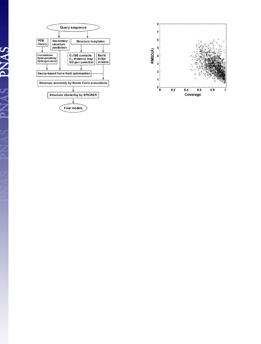
The protein structure modeling procedure used in this work consists
of template identification, force field construction, fragment as-
sembly, and model selection. A flowchart is presented in Fig. 1.

Template Identification.

Templates are identified from the solved

structures in the PDB by structurally aligning the native of query
proteins to templates by using our Structure Alignment (

SAL

algorithm (20). The alignment is performed by a Needleman–

Abbreviations: RMSD, rms deviation; SG, side-chain group; FJC, freely jointed chain.

*To whom correspondence should be addressed. E-mail: [e-mail].

© 2005 by The National Academy of Sciences of the USA

www.pnas.org

兾cgi兾doi兾10.1073兾pnas.0407152101

PNAS

兩 January 25, 2005 兩 vol. 102 兩 no. 4 兩 1029–1034

BIOPHYSICS

Wunsch dynamic program (28) with the score matrix defined as (29)
score(i, j)

⫽ 20兾(1 ⫹ d

ij

3

兾5), where d

ij

is the spatial distance between

the ith and jth residues after an initial guessed superposition. A
number of iterations are performed until the structure alignment
converges. Various gap penalties are implemented, and the best
alignment is selected on the basis of the Z-score of the relative
RMSD of two aligned proteins (30).

Force Field Construction.

The force field used in

TASSER

includes

four classes of terms: (i) C

␣

and side-chain group (SG) regularities

兾

correlations from the statistics of the PDB, (ii) propensities for
predicted secondary structure from

PSIPRED

(31), (iii) tertiary

consensus contact

兾distance restraints, and (iv) a protein-specific

SG pair potential, both extracted from the identified multiple
templates. The construction and implementation of the potentials
in i and ii have been described (32, 33). The tertiary restraints in iii
are constructed as done by our threading program

PROSPECTOR

㛭

3

(6); and the details of the new pair potential in iv are in the
Appendix.

Having all of the energy terms, optimization for the combination

weight factors was performed based on 100 training proteins
(outside the benchmark test set used here), each with 60,000
structure decoys, where we maximize the correlation between the
energy and RMSD from native to the decoys (32).

Structure Assembly.

Full-length models are constructed by reassem-

bling the continuous fragments excised from the templates under
the guide of the optimized force field. These fragments are ele-
mental building blocks with internal conformations kept invariant
during modeling. Residues in gapped regions are generated from an
ab initio lattice modeling approach (32). These regions also serve as
linkage points for the rigid block movements. Conformational
space is searched by using parallel hyperbolic Monte Carlo sampling
(34), where the tertiary topology varies by continuous translations
and rotations of the rigid blocks. The magnitude of the move is
scaled by the size of the blocks. Forty to fifty replicas are used in the
simulations depending on protein size, and the trajectories in the 14
lowest temperature replicas are submitted to

SPICKER

(35) for

clustering. The final models are combined from members of the
structure clusters, ranked on the basis of cluster structure density.

Results and Discussion

Benchmark of Targets and Templates.

For test proteins, we develop

a representative benchmark set of all single-domain structures in
PDB with 41–200 aa. This target set contains 1,489 nonhomologous
proteins having 448, 434, and 550

␣-, ␤-, and ␣␤-proteins, respec-

tively (the other 57 are C

␣

-only targets or have irregular secondary

structures). The template library consists of 3,575 representative
proteins from the PDB with a maximum 35% pairwise sequence
identity to each other; all templates are taken from this library.

Fig. 2 shows a summary of the resulting templates that have the

highest RMSD Z-score obtained from

SAL

(20) for all 1,489 test

proteins, where all templates with

⬎25% sequence identity to the

target protein are excluded. The majority of targets have

⬎70%

coverage and

⬍4-Å RMSD to native, which shows the significant

denseness of protein structure space. The average sequence identity
between template and target is 13% in the aligned regions.

Summary of Folding Results.

Table 1 presents a summary of the

folding results, where, for each protein, the two templates with the
highest RMSD Z-score are used in

TASSER

. A detailed list of

templates and final models, as well as the simulation trajectories,
can be obtained by contacting J.S.

In Table 1, the second column shows the best templates in the top

two with the lowest RMSD to native in the aligned regions. On
average, the RMSD to native is 2.51 Å with 82% coverage. The final
models show improvement over the initial template alignments.
Over the same aligned regions, the average RMSD to native is
reduced to 1.88 Å. Many low-resolution templates have been shifted
by

TASSER

refinement to structures with an acceptable resolution

for biochemical function annotation (24). For example, there are
358 targets shifted from

⬎3-Å to ⬍3-Å RMSD to native, and 424

targets shifted from above to below 2 Å.

For full-length models, almost all targets (except for 1a2kC and

1k5dB) have an RMSD to native below 6 Å for the best of the top
five models, with an average rank of 1.7; 97% have an RMSD

⬍4

Å. The average RMSD to native is 2.25 Å, comparable with the
accuracy of a low-resolution NMR or x-ray structure (25, 36, 37).
For the rank one cluster that has the highest structure density, the
average RMSD to native is 2.35 Å.

As a reference, we also list in the right hand columns of Table

1 the results of refined models from the publicly available
comparative modeling program

MODELLER

(2, 3), using the same

templates from

SAL

. The average RMSD of the best of top five

models by

MODELLER

is 3.74 Å (average rank of 2.9; here, the

rank of

MODELLER

models is decided by their objective function),

with 2.71 Å in the aligned regions. In general, successful

Fig. 1.

Overview of the

TASSER

structure prediction methodology that con-

sists of template identification (here by structure alignment), force field
construction, structure assembly, and model selection.

Fig. 2.

RMSD to native of the templates identified by the structure alignment

program

SAL

(20) versus the alignment coverage.

1030

兩 www.pnas.org兾cgi兾doi兾10.1073兾pnas.0407152101

Zhang and Skolnick

modeling in

MODELLER

has a stronger dependence on the

template coverage than in

TASSER

. For example, if we look at

those targets with

⬎90% coverage (437 in total), the average

RMSDs of the full-length models by

TASSER

and

MODELLER

are

fairly close, i.e., 1.56 Å and 2.19 Å, respectively. However, for
targets with initial alignment coverage

⬍75% (386 in total), the

average RMSDs from native to models using

TASSER

and

MODELLER

are 2.92 Å and 6.05 Å, respectively, a significant

difference. Overall, in 1,120 targets,

TASSER

models have a lower

RMSD to native, where the alignment coverage in those targets
is on average 81%. For 102 targets,

MODELLER

does better,

where the coverage is on average 92%. Nevertheless, both
procedures lead to the conclusion that the structure alignments
produced by

SAL

can produce buildable models.

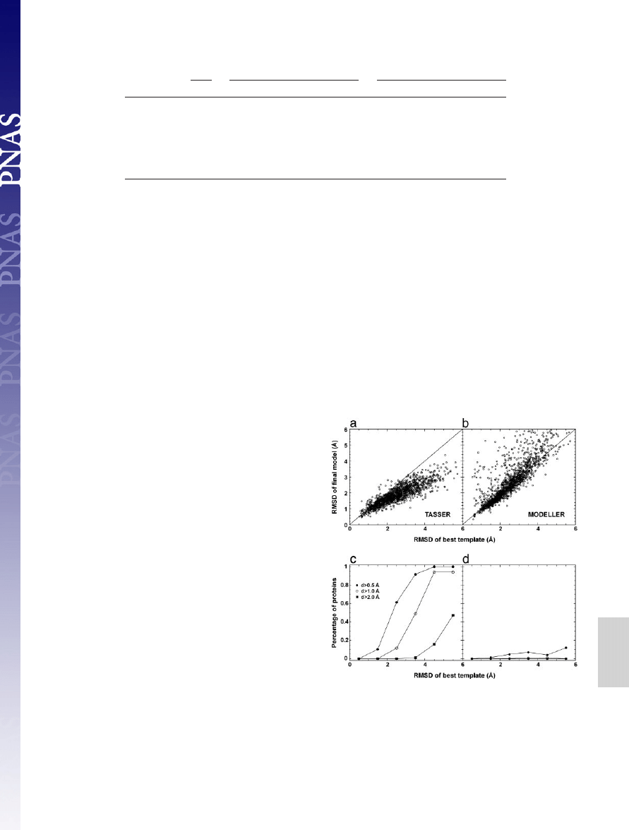
Improvements of Initial Alignment.

In Fig. 3, we plot a detailed

comparison of the final models with respect to the template in the
aligned regions. In the majority of cases,

TASSER

models show

obvious improvement (see Fig. 3a). As shown in Fig. 3c, for targets
having initial templates of aligned regions with an RMSD ranging
from 2 to 3 Å, for

⬇61% of these cases, the models have at least a

0.5-Å improvement; and for initial alignments with an initial RMSD
from 3 to 4 Å, in

⬇49% of cases, the final models improve by at least

1.0 Å. This result is partly because the force field takes consensus
information from multiple templates, which can have higher accu-
racy

兾confidence than that from individual templates. In

TASSER

,

the local fragments from individual templates are rearranged under
the guide of the force field, and the global topology can therefore
move closer to native. This consensus information is further rein-
forced during the final model combination procedure of

SPICKER

clustering (35). Another factor that contributes to the improvement
is the protein-like energy terms, representing an optimal combina-
tion of statistical potentials, hydrogen bonds, and secondary struc-
ture predictions that lead to better side-chain and backbone struc-
ture packing than in the initial template-based alignments (27, 32).

In Fig. 3 b and d, we also show the comparison between the

models generated by

MODELLER

and the initial template align-

ments. In the majority of cases,

MODELLER

keeps the topology of

models near the template, which is understandable because it was
designed to optimally satisfy the spatial restraints from templates
for homologous proteins (2, 3). However, in a few cases (

⬇10%),

the

MODELLER

models can be

⬎1 Å worse than the initial templates.

Modeling Unaligned

兾Loop Regions.

Because there is no spatial

information provided from the template alignments, modeling the
unaligned or loop regions is a hard, unsolved problem (3, 38, 39).
Here, we define an unaligned or loop region (including tails) as a
piece of continuous sequence that has no coordinate assignment in
the

SAL

template alignments. For each piece of those sequences,

two types of accuracy are calculated (3): RMSD

local

denotes the

RMSD between native and the modeled loop with direct super-
position of the unaligned region; RMSD

global

is the RMSD between

native and modeled loop after superposition of up to five neigh-
boring stem residues on each side of the loop (for tails, the
supposition is done on the side including five stem residues).
RMSD

local

measures the modeling accuracy of the local conforma-

tion, whereas RMSD

global

measures both the accuracy of the local

conformation and the global orientation.

There are in total 11,380 unaligned

兾loop regions with size from

1–84 residues in the 1,489 targets. In Fig. 4, we show the average
values of RMSD

local

and RMSD

global

of

TASSER

and

MODELLER

models versus loop length L. In both cases, the accuracy of loop

Table 1. Summary of templates by

SAL

(20) and models built by

TASSER

or

MODELLER

(2,3)

SAL

TASSER

MODELLER

Best*

Align

†

Top five

‡

Top one

§

Align

†

Top five

‡

Top one

§

RMSD, Å

2.510

1.877

2.246

2.352

2.708

3.740

4.318

Coverage, %

82

82

100

100

82

100

100

N

RMSD

⬍6

¶

1,489

1,489

1,487

1,481

1,462

1,326

1,202

N

RMSD

⬍5

1,472

1,489

1,481

1,464

1,395

1,195

1,060

N

RMSD

⬍4

1,369

1,488

1,447

1,423

1,255

984

841

N

RMSD

⬍3

1,064

1,422

1,259

1,206

1,008

647

551

N

RMSD

⬍2

498

922

623

582

520

300

244

N

RMSD

⬍1

46

83

52

49

37

20

15

*The template of the lowest RMSD to native.

†

The best model in top five by

TASSER

and

MODELLER

with the RMSD calculated in the aligned region.

‡

The best model in top five where the RMSD is calculated for the entire chain.

§

The first model where the RMSD is calculated for the entire chain.

¶

No. of targets with RMSD below the specified threshold (Å).

Fig. 3.

Comparison of initial and final alignments to the target structure. (a)

Scatter plot of RMSD from native of the final models built by

TASSER

refinements

versus RMSD from native of the initial template alignments identified by

SAL

. The

same aligned regions are used in both RMSD calculations. (b) Similar data as in a,
but the models are from

MODELLER

refinements. (c) Fraction of targets with an

RMSD improvement ‘‘d’’ by

TASSER

greater than some threshold value. Here d

⫽

(RMSD of template)

⫺ (RMSD of final model), where both RMSDs are calculated

over aligned regions. Each point in c is calculated with a bin width of 1 Å. (d)
Similar data as in c, but the models are from

MODELLER

.

Zhang and Skolnick

PNAS

兩 January 25, 2005 兩 vol. 102 兩 no. 4 兩 1031

BIOPHYSICS

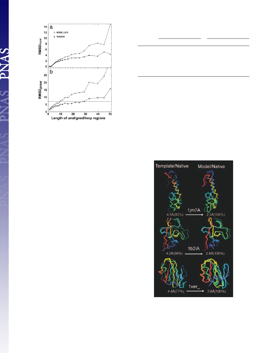
modeling decreases with increasing loop size. However, for all size
ranges, the loops in

TASSER

models have lower average RMSD

local

and RMSD

global

. If we make a cutoff of RMSD

global

⬍7 Å in Fig.

4b,

MODELLER

generates reasonable models for unaligned

兾loop

regions of length up to 10 residues;

TASSER

can have the same

accuracy cutoff for the loops up to 28 residues. If using a lower
RMSD

global

cutoff, the acceptable loop size in both approaches will

decrease, and the difference between

MODELLER

and

TASSER

becomes smaller.

Most unaligned regions

兾loops in

SAL

alignments are of small size,

which are relatively easier to model because of the limited config-
uration entropy. If we focus only on the unaligned loops of length
greater than or equal to four residues, there are 1,675 cases with an
average length of 8.8 residues. The distribution of modeling accu-
racy is summarized in Table 2. Consistent with Fig. 4a, the
distribution of RMSD

local

is quite close using

TASSER

and

MOD

-

ELLER

. However,

TASSER

shows an obviously better control of loop

orientations. For example, in one-third (549

兾1,675) of the cases,

including loops and tails,

TASSER

generates models of RMSD

global

⬍3 Å, whereas the fraction of

MODELLER

models having

RMSD

global

⬍3 Å is around one-seventh (244兾1,675).

Representative Examples.

In Fig. 5, three representative examples of

TASSER

modeling results are provided: 1jm7A (an

␣-protein), 1b2iA

(a

␤-protein), and 1xer (an ␣␤-protein). In all three, the template

topologies in the core identified by

SAL

are quite similar to native

(

⬍5 Å); however, the local packing of the fragments and sometimes

the termini are misoriented. Rearrangement using the

TASSER

force

field results in a

⬎2 Å improvement in the aligned region.

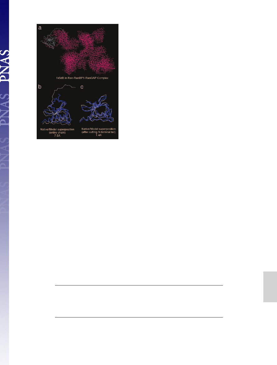
In Fig. 6, we show the predicted structure of 1k5dB, one of the

two cases where

TASSER

failed to generate models with an RMSD

to native below 6 Å. This is a Ran-binding protein (Ran-BP1), i.e.,
chain B of the Ran-RanBP1–RanGAP protein complex (40), which
has a long tail interacting with chain A (Ran). Because interactions
with partner chains are not included, we failed to model the
configuration of the tail; this case results in a full-length RMSD of
7.8 Å to native. If we cut the first 22 residues in the N terminus
associated with intermolecular interactions, the core region of the
first model has a 1.4-Å RMSD (Fig. 6c).

New Fold Targets in CASP5.

We revisit the new fold targets in the

CASP5 folding experiment (10), because, by definition, those
targets putatively adopt a novel tertiary topology (1). However, as
shown in Table 3, there are still more or less similar folds found in
PDB, although the sequence identity is very low (

⬇7% on average).

The new entries in PDB released later than the CASP5 prediction
season are not included in our template library. On average, these
templates have shorter alignments (

⬇73% coverage) with higher

RMSD (

⬇3.8 Å) than those identified for the benchmark proteins.

Still, acceptable models can be built from the initial template
alignments using

TASSER

, with an average RMSD from native of

2.87 Å for the first predicted model.

Table 2. Result of modeling of unaligned

兾loop regions

(>4 residues) by

TASSER

and

MODELLER

TASSER

MODELLER

RMSD

local

*

RMSD

global

*

RMSD

local

*

RMSD

global

*

N

RMSD

⬍6

†

1,670

1,386

1,633

1,011

N

RMSD

⬍5

1,664

1,199

1,603

800

N

RMSD

⬍4

1,631

924

1,528

507

N

RMSD

⬍3

1,527

549

1,342

244

N

RMSD

⬍2

1,173

193

1,009

64

N

RMSD

⬍1

519

18

498

10

RMSD, Å

1.62

4.34

2.02

6.59

*See text for definitions of RMSD

local

and RMSD

global

.

†

No. of targets with a RMSD below the specified threshold (Å).

Fig. 4.

RMSD

local

(a) and RMSD

global

(b) of unaligned

兾loop regions as a

function of loop length (L).

TASSER

and

MODELLER

models are denoted by

triangles and circles, respectively. The lines connecting the points serve to
guide the eye. The dashed line in b denotes an RMSD

global

cutoff of 7 Å.

Fig. 5.

Representative examples showing the improvement of final models

with respect to their initial template alignments. The left column is the
superposition of the template alignments and native, and the right column is
that for refined models and native. The thin lines are native structures; the
thick lines signify templates or final models. Blue to red runs from N to C
terminus. The numbers in parentheses are the coverage of the templates or
models on which the denoted RMSD has been calculated.

1032

兩 www.pnas.org兾cgi兾doi兾10.1073兾pnas.0407152101

Zhang and Skolnick

Concluding Remarks
In this article, we examined the issues of whether all single-domain
proteins are foldable based on the set of solved structures currently
deposited in PDB (1) and whether the templates can be further
improved by rearranging the fragments. We used our structure
alignment algorithm,

SAL

(20), to identify the best possible target–

template pairs, and then attempted to build and refine the full-
length model using the template assembly

兾refinement algorithm

TASSER

(27). This strategy was applied to a comprehensive PDB

benchmark set of 1,489 medium-size, single-domain proteins. With
homologous proteins excluded, similar folds can be found for all
benchmark proteins, and the majority have a RMSD to native

⬍4

Å over

⬎70% of their sequence. On average, the RMSD between

template and native is 2.51 Å with

⬇82% alignment coverage. After

TASSER

, the average RMSD in the aligned region improves to 1.88

Å. The average global RMSD of unaligned

兾loop兾tail regions (ⱖ4

residues) generated by

TASSER

is 4.3 Å. Almost all targets have at

least one full-length model in the top five with an RMSD to native

below 6 Å (97% are below 4 Å). The average RMSD to native is
2.25 Å, comparable with the accuracy of low-to-moderate-
resolution experimental structures. In this sense, the answer to the
question of completeness of the current PDB library for model
construction of single-domain proteins is quite positive. Not only
can physically reasonable models be built, but, starting from struc-
tural alignments, there is a significant improvement in many
models; 349

兾1,489 targets have a RMSD improvement of ⬎1.0 Å

in the aligned region. Thus, it is suggestive that the barrier to
structure refinement noted in CASP5 (10) has been broken.

In contrast to previous approaches, there are several reasons that

contribute to the improvement of model quality compared with
initial templates. First, the force field includes multiple sources of
knowledge-based potentials and consensus tertiary restraints from
multiple templates. The consensus spatial information usually has
higher accuracy

兾confidence than that of individual templates.

Second, the combination of the different types of energy terms was
optimized on the basis of a large-scale set of structure decoys
(including 100

⫻ 60,000 extrinsic targets兾structures) to yield an

optimized potential that can provide better packing of the side-
chains and peptides. This improvement occurs because of a better
correlation between model quality and energy (the correlation
coefficient between RMSD and the combined potential for test
cases is

⬇0.7). Finally, templates usually contain unphysical align-

ments because chain connectivity was not considered in the initial
alignments. The reassembly procedure of

TASSER

that converts

these unphysical alignments into physical models also contributes to
the improvement in model quality relative to that of the initial
template alignment. Unlike many other comparative modeling
approaches, e.g.,

MODELLER

(2), whose goal is to optimally satisfy

the spatial restraints of an initial template, the relative orientation
of template fragments, and therefore global topology in

TASSER

models, can change. On the other hand, the local conformation of
the continuous fragments is kept rigid during the modeling proce-
dure, which helps the models retain the accuracy of well-aligned
regions from native and reduces the conformational entropy.

For the more realistic situation where templates

兾alignments are

identified by using our threading program

PROSPECTOR

㛭

3

(6), the

success rate for the same benchmark set of targets proteins is about
two-thirds (where a foldable case is defined if one of top five
full-length models has an RMSD below 6.5 Å to native) (27). The
results reported here highlight the urgent need to develop more
efficient fold recognition algorithms that can provide acceptable
templates for the remaining one-third of proteins, as well as better
alignments to improve the overall quality of the predictions. In
previous work (27), we also observed an improvement in the models
relative to their initial template alignments, but because threading
models tend to be of poorer quality than those obtained from
structural alignments, it could be argued that the results are not that
significant (i.e., the predicted models might be poorer than the best
structural alignments). Here we have demonstrated that even when

Fig. 6.

A representative example of targets where the final model has an

RMSD to native

⬎6 Å. The native structure of 1k5dB is shown in white with thin

backbones; the predicted model of the highest cluster density in blue with
thick backbones. The red wire-frame in a denotes the partner chains in the
Ran-RanBP1–RanGAP complex. (a) 1k5dB in the entire complex. (b) Native
model superposition. (c) As in b but with the tail cut off.

Table 3. Folding results for the new fold targets in CASP5

PDB ID

CASP5 ID

Length

RT

ali

, Å* (%)

RM

ali

, Å

†

R5, Å

‡

R1, Å

§

1h40

㛭

T0170

69

2.81 (83)

1.57

1.70 (2)

1.79

1iznC

T0162

㛭3

168

5.82 (61)

3.28

3.05 (2)

3.31

1m6yB

T0172

㛭2

101

3.31 (71)

2.62

2.79 (1)

2.79

1nyn

㛭

T0181

111

5.10 (74)

3.88

3.94 (1)

3.94

1o0uB

T0187

㛭1

165

3.61 (56)

3.10

3.56 (1)

3.56

1o12C

T0186

㛭3

36

2.16 (94)

1.71

1.82 (1)

1.82

Average

108.3

3.80 (73)

2.69

2.81 (1.3)

2.87

ali, aligned.

*RMSD to native of the best template (RT) and the alignment coverage.

†

RMSD from the final model (RM) to native over initial aligned regions.

‡

RMSD to native for the best model in the top five. The number in parentheses is the rank of the best model.

§

RMSD to native for the rank-one model.

Zhang and Skolnick

PNAS

兩 January 25, 2005 兩 vol. 102 兩 no. 4 兩 1033

BIOPHYSICS

the best structural alignments are used, we can often improve the
models. This demonstration represents significant progress in the
field.

Because the average sequence identity between the target pro-

teins and the best templates identified here is only

⬇13%, much

lower than the ‘‘twilight zone’’ of sequence identity, correctly
aligning the sequence to these templates will be a major challenge.
This result is certainly true for our threading program,

PROSPEC

-

TOR

㛭

3

, where for

⬇90% of targets, at least one correct fold can be

identified in a large scale test; however, only around 62% were
aligned correctly (6).

The results reported here provide a lower bound to the com-

pleteness and utility of the current PDB library. Certainly, the
structure alignment program

SAL

is not perfect. It is not guaranteed

to find the best structural alignment because the final alignment in
this algorithm is sensitive to the initial guessed superposition. In

recent work (unpublished results), we found that using the align-
ment from other software [in particular,

CE

(14)] as the initial

alignment in

SAL

results in structure alignments of longer coverage

and lower RMSD to native. Better structure alignment algorithms
only serve to identify better templates from the PDB, which should
result in better final models than reported here. Nevertheless, even
now, it seems that the library of the solved protein structures is
complete at the level of single-domain proteins. This structure
completeness should have significant implications for both protein
structure prediction and structural genomics (21, 23).

Appendix: Multiple-Template-Based SG Pair Potential
The protein-specific pair potential in our force field (term iv in the
potential) is calculated from the identified multiple templates by
using

V

共i, j兲

⫽

再

⫺ ln

q

共i, j兲

Q

共i, j兲q

0

共i, j, N兾L兲 ⫹

具

ln

q

共i, j兲

Q

共i, j兲q

0

共i, j, N兾L兲

典

0

if

共i, j兲 are in aligned regions

if

共i, j兲 are in gapped regions,

[1]

where q(i, j) is the number of SG contacts between residues i and
j in all of the templates; Q(i, j) is the number of templates that have
both residue i and j aligned; and q

0

(i, j, N

兾L) is the expected

probability of contacts between residues i and j for a random chain
of size L having a given total contact number N. The average

具. . .典

is over all aligned pairs of (i, j); the shift sets the potential in gapped
regions equal to the average magnitude of that in the aligned
regions.

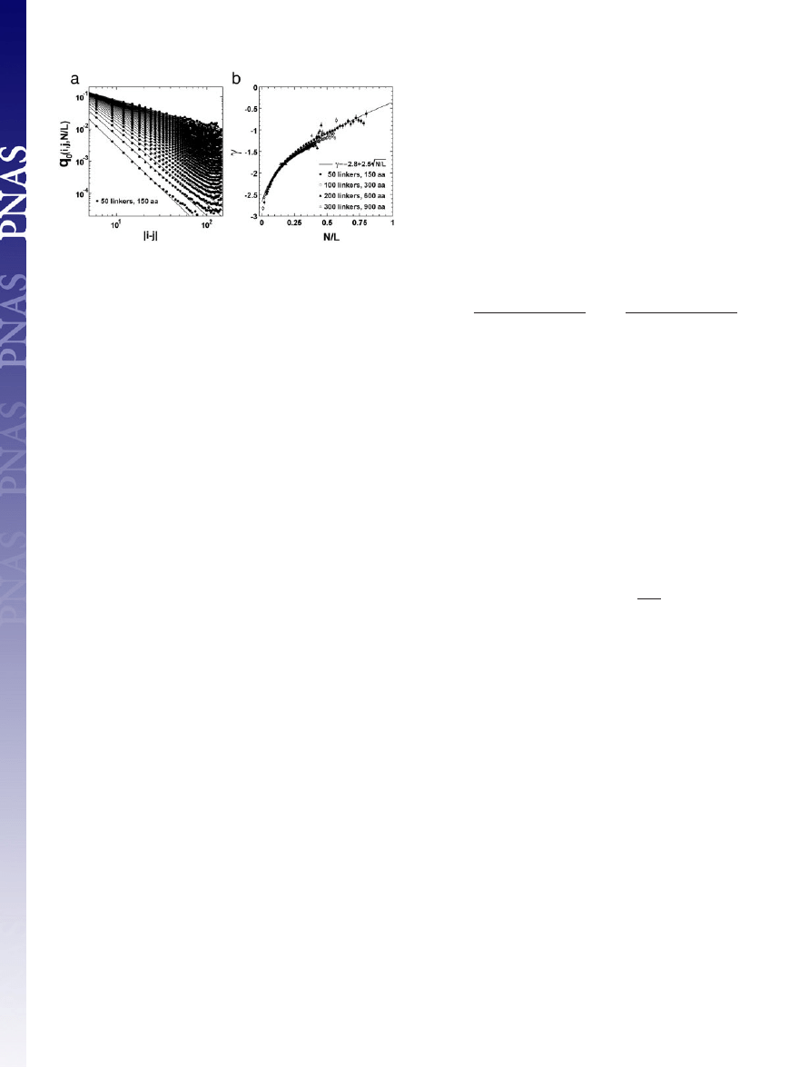
To calculate q

0

(i, j, N

兾L), we performed a Monte Carlo calcu-

lation of the freely jointed chain (FJC) model (41, 42) with excluded
volume. Fig. 7a shows the result for q

0

(i, j, N

兾L) from a random

chain of 50 linkers. The contact probability of the FJC follows a
power-law over more than three orders of magnitude: q

0

(i, j,

N

兾L) ⬇ 兩i ⫺ j兩

␥(N/L)

. Similar results are also obtained from the chains

with 100, 200, and 300 linkers (data not shown). In Fig. 7b,

␥ as a

function of different scaled contact-numbers, (N

兾L), is presented.

The data are well fit by:

␥ ⫽ ⫺2.8 ⫹ 2.5公N兾L.

Integration of the contact probability results in a power-law: P(i,

j)

⬅ 兺

N/L

q

0

(i, j, N

兾L) ⬃ 兩i ⫺ j兩

⫺1.84

, which coincides with the

estimate from a Gaussian random chain with excluded volume that
has a power of

⫺9兾5 (41).

This research was supported in part by National Institutes of Health
Grants GM-37408 and GM-48835.

1. Berman, H. M., Westbrook, J., Feng, Z., Gilliland, G., Bhat, T. N., Weissig, H.,

Shindyalov, I. N. & Bourne, P. E. (2000) Nucleic Acids Res. 28, 235–242.

2. Sali, A. & Blundell, T. L. (1993) J. Mol. Biol. 234, 779–815.
3. Fiser, A., Do, R. K. & Sali, A. (2000) Protein Sci. 9, 1753–1773.
4. Bowie, J. U., Luthy, R. & Eisenberg, D. (1991) Science 253, 164–170.
5. Jones, D. T. (1999) J. Mol. Biol. 287, 797–815.
6. Skolnick, J., Kihara, D. & Zhang, Y. (2004) Proteins 56, 502–518.
7. Bryant, S. H. & Altschul, S. F. (1995) Curr. Opin. Struct. Biol. 5, 236–244.
8. Moult, J., Hubbard, T., Fidelis, K. & Pedersen, J. T. (1999) Proteins 37, Suppl. 3, 2–6.
9. Moult, J., Fidelis, K., Zemla, A. & Hubbard, T. (2001) Proteins 45, Suppl. 5, 2–7.

10. Moult, J., Fidelis, K., Zemla, A. & Hubbard, T. (2003) Proteins 53, Suppl. 6, 334–339.
11. Taylor, W. R., Flores, T. P. & Orengo, C. A. (1994) Protein Sci. 3, 1858–1870.
12. Holm, L. & Sander, C. (1995) Trends Biochem. Sci. 20, 478–480.
13. Gibrat, J. F., Madej, T. & Bryant, S. H. (1996) Curr. Opin. Struct. Biol. 6, 377–385.
14. Shindyalov, I. N. & Bourne, P. E. (1998) Protein Eng. 11, 739–747.
15. Holm, L. & Sander, C. (1996) Science 273, 595–603.
16. Murzin, A. G., Brenner, S. E., Hubbard, T. & Chothia, C. (1995) J. Mol. Biol. 247,

536–540.

17. Orengo, C. A., Michie, A. D., Jones, S., Jones, D. T., Swindells, M. B. & Thornton,

J. M. (1997) Structure 5, 1093–1108.

18. Yang, A. S. & Honig, B. (2000) J. Mol. Biol. 301, 665–678.
19. Harrison, A., Pearl, F., Mott, R., Thornton, J. & Orengo, C. (2002) J. Mol. Biol. 323,

909–926.

20. Kihara, D. & Skolnick, J. (2003) J. Mol. Biol. 334, 793–802.
21. Skolnick, J., Fetrow, J. S. & Kolinski, A. (2000) Nat. Biotechnol. 18, 283–287.
22. Baxter, S. M. & Fetrow, J. S. (2001) Curr. Opin. Drug Discov. Devel. 4, 291–295.

23. Baker, D. & Sali, A. (2001) Science 294, 93–96.
24. Arakaki, A. K., Zhang, Y. & Skolnick, J. (2004) Bioinformatics 20, 1087–1096.
25. Marti-Renom, M. A., Stuart, A. C., Fiser, A., Sanchez, R., Melo, F. & Sali, A. (2000)

Annu. Rev. Biophys. Biomol. Struct. 29, 291–325.

26. Tramontano, A. & Morea, V. (2003) Proteins 53, Suppl. 6, 352–368.
27. Zhang, Y. & Skolnick, J. (2004) Proc. Natl. Acad. Sci. USA 101, 7594–7599.
28. Needleman, S. B. & Wunsch, C. D. (1970) J. Mol. Biol. 48, 443–453.
29. Gerstein, M. & Levitt, M. (1996) Proc. Int. Conf. Intell. Syst. Mol. Biol. 4, 59–67.
30. Betancourt, M. R. & Skolnick, J. (2001) J. Comp. Chem. 22, 339–353.
31. Jones, D. T. (1999) J. Mol. Biol. 292, 195–202.
32. Zhang, Y., Kolinski, A. & Skolnick, J. (2003) Biophys. J. 85, 1145–1164.
33. Kolinski, A. & Skolnick, J. (1998) Proteins 32, 475–494.
34. Zhang, Y., Kihara, D. & Skolnick, J. (2002) Proteins 48, 192–201.
35. Zhang, Y. & Skolnick, J. (2004) J. Comput. Chem. 25, 865–871.
36. Glusker, J. P. (1994) Methods Biochem. Anal. 37, 1–72.
37. Wagner, G., Hyberts, S. G. & Havel, T. F. (1992) Annu. Rev. Biophys. Biomol. Struct. 21,

167–198.

38. Mosimann, S., Meleshko, R. & James, M. N. (1995) Proteins 23, 301–317.
39. Martin, A. C., MacArthur, M. W. & Thornton, J. M. (1997) Proteins 29, Suppl. 1,

14–28.

40. Seewald, M. J., Korner, C., Wittinghofer, A. & Vetter, I. R. (2002) Nature 415, 662–666.
41. Doi, M. & Edwards, S. F. (1986) The Theory of Polymer Dynamics (Clarendon Press,

Oxford).

42. Zhang, Y., Zhou, H. J. & Ouyang, Z. C. (2001) Biophys. J. 81, 1133–1143.
43. Rief, M., Fernandez, J. M. & Gaub, H. E. (1998) Phys. Rev. Lett. 81, 4764–4767.

Fig. 7.

Side-chain contact probability for random chains as a function of

chain length. (a) Contact probability q

0

(i,j,N

兾L) for the ith and jth residues at

given scaled contact-numbers, N

兾L, versus the distance 兩i ⫺ j兩 along the protein

chain, from simulations of an FJC of 50 linkers with excluded volume. The
Kuhn-length of the FJC is taken to be 11.4 Å, according to experimental single
protein molecule stretching data (43). The definition of excluded volume is
introduced on the basis of the minimal observed C

␣

distance in the PDB, i.e.,

no pair of linkers of the FJC could go closer than 4.5 Å. Contacts are defined
based on a weighted average of C

␣

distances for contacting residues in the

PDB, i.e., a contact occurs if two linkers are closer than 7.27 Å. The curves are
the least square fits to the power-law at each given N

兾L. (b) The power

␥ versus

the scaled contact-number N

兾L. Data are from the FJC of different lengths, i.e.,

50-, 100-, 200-, and 300-residue linkers, which correspond to the protein
lengths of 150, 300, 600, and 900 residues, respectively, because one Kuhn-
length here corresponds approximately to three C

␣

–C

␣

backbone lengths. The

error bars denote the power-law fitting errors of a. The curve denotes the least
square fit equation:

␥ ⫽ ⫺2.8 ⫹ 2.5公N兾L.

1034

兩 www.pnas.org兾cgi兾doi兾10.1073兾pnas.0407152101

Zhang and Skolnick