Curbing Bailouts

New Comparative politiCs

Series Editor
michael laver, New York University

Editorial Board
Ken Benoit, trinity College, Dublin
Gary Cox, University of California, san Diego
simon Hix, london school of economics
John Huber, Columbia
Herbert Kitschelt, Duke
w. Bingham powell, rochester
Kaare strøm, University of California, san Diego
George tsebelis, University of michigan
leonard wantchekon, New York University

the New Comparative politics series brings together cutting-edge work on social

conflict, political economy, and institutional development. Whatever its substantive
focus, each book in the series builds on solid theoretical foundations; uses rigorous
empirical analysis; and deals with timely, politically relevant questions.

Curbing Bailouts: Bank Crises and Democratic Accountability in
Comparative Perspective
Guillermo rosas

Curbing Bailouts

Bank Crises and Democratic Accountability in
Comparative Perspective

Guillermo Rosas

The University of Michigan Press

Ann Arbor

Copyright © by the University of michigan 2009
all rights reserved
published in the United states of america by
the University of michigan press
manufactured in the United states of america
c

printed on acid-free paper

2012 2011 2010 2009 4 3 2 1

No part of this publication may be reproduced,
stored in a retrieval system, or transmitted in any form
or by any means, electronic, mechanical, or otherwise,
without the written permission of the publisher.

A CIP catalog record for this book is available from the British Library.

U.S. CIP data on file.

isBN 978-0-472-11713-0 (cloth : alk. paper)

ISBN 978-0-472-02236-6 (electronic)

Para Tabea, Aitana y Emilio

Contents

List of Tables

List of Figures

List of Acronyms

Preface and Acknowledgments

xiii

Bagehot or Bailout?
Policy Responses to Banking Crises

Accidents Waiting to Happen

Political Regimes, Bank Insolvency,
and Closure Rules

Argentina and Mexico:

A Closer Look at Bank Bailouts

Variation in Government Bailout Propensities

Political Regimes and Bailout Propensities

116

Political Regimes and Banking Crises

145

Conclusion

171

Appendices

178

References

187

Index

199

List of Tables

2.1

Balance sheet of a solvent bank . . . . . . . . . . . . . . . .

2.2

Balance sheet of an insolvent bank . . . . . . . . . . . . . .

2.3

Responses to banking crises in ﬁve policy arenas

. . . . . .

3.1

Balance sheet of model bank assuming no deposit withdrawals 33

3.2

Balance sheet after depositor run, support, and project success 35

3.3

Payo

ﬀs for entrepreneurs and depositors . . . . . . . . . . . 36

3.4

Model assumptions . . . . . . . . . . . . . . . . . . . . . .

4.1

Survival of Argentine banks

. . . . . . . . . . . . . . . . .

4.2

Survival of Mexican banks . . . . . . . . . . . . . . . . . .

4.3

Exponential models of bank survival . . . . . . . . . . . . .

4.4

Weibull models of bank survival . . . . . . . . . . . . . . .

5.1

Empirical indicators of seven crisis-management policies . .

5.2

Estimates of IRT bailout propensity model . . . . . . . . . . 103

5.3

Predicted implementation of crisis-management policies (I)

111

6.1

Estimates of government-level parameters . . . . . . . . . . 126

6.2

Statistics for balanced and unbalanced samples . . . . . . . 129

6.3

Causal interpretation of government parameter estimates . . 132

6.4

Estimates of two-dimensional IRT model

. . . . . . . . . . 140

6.5

Predicted implementation of crisis-management policies (II)

143

7.1

Breakdown of events by regime and wealth . . . . . . . . . 149

7.2

Ordinal logit model of banking crises

. . . . . . . . . . . . 155

7.3

Predicted count of banking crises across regimes

. . . . . . 160

7.4

Aggregate balance of banking system

. . . . . . . . . . . . 161

7.5

Breakdown of net worth by regime and wealth . . . . . . . . 163

7.6

Models of aggregate net worth . . . . . . . . . . . . . . . . 166

List of Figures

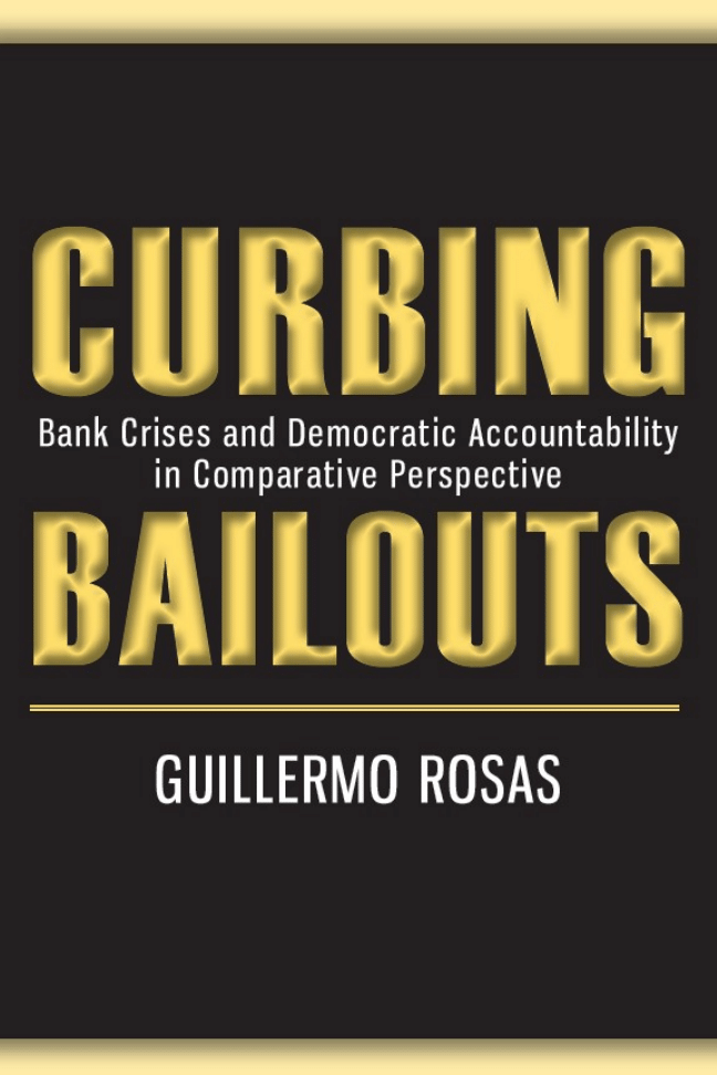
3.1

Extensive form of the banking crisis game . . . . . . . . . .

3.2

Bank closure under a benevolent government . . . . . . . .

3.3

Choice of risk proﬁle and closure rule . . . . . . . . . . . .

3.4

Size of crony contract and ex ante probability of failure . . .

3.5

Equilibrium outcomes under the assumption of systemic risk

4.1

Alternative modes of bank continuation or exit . . . . . . . .

4.2

Kaplan-Meier estimates of bank survival . . . . . . . . . . .

5.1

Parameters of policy di

ﬃculty and bailout propensity . . . . 104

5.2

Item response curves and probability of policy enactment . . 107

5.3

Estimates of government bailout propensities . . . . . . . . 109

6.1

Propensity scores of democracies and non-democracies . . . 130

6.2

Predictive distribution of bailout scores across regimes . . . 135

6.3

Bailout propensity scores across regimes . . . . . . . . . . . 141

7.1

Posterior distribution of random e

ﬀects . . . . . . . . . . . . 156

7.2

Predictive distribution of distress across regimes . . . . . . . 158

7.3

Aggregate net worth series for Argentina and Mexico . . . . 162

7.4

Predictive distribution of net worth across regimes . . . . . . 168

7.5

Added-variable plots of country-speciﬁc intercept and vari-
ance parameters . . . . . . . . . . . . . . . . . . . . . . . . 169

List of Acronyms

AdeBA

Asociaci´on de Bancos de Argentina

Banxico

Banco de M´exico

BCRA

Banco Central de la Rep´ublica Argentina

BNA

Banco de la Naci´on Argentina

CAR

capital-asset ratio

CMHN

Consejo Mexicano de Hombres de Negocios

CNBV

Comisi´on Nacional Bancaria y de Valores

ECB

European Central Bank

FFCB

Fondo Fiduciario de Capitalizaci´on Bancaria

Fobaproa

Fondo Bancario de Protecci´on al Ahorro

Fogade

Fondo de Garant´ıa de Dep´ositos

IFS

International Financial Statistics

IMF

International Monetary Fund

INEGI

Instituto Nacional de Estad´ıstica, Geograf´ıa e Inform´atica

IPAB

Instituto de Protecci´on al Ahorro Bancario

Libor

London Interbank O

ﬀered Rate

LOLR

lender of last resort

MCMC

Markov chain Monte Carlo

MECON

Ministerio de Econom´ıa

xii

List of Acronyms

NPL

non-performing loans

P&A

Purchase and Assumption

Procapte

Programa de Capitalizaci´on Permanente

SHCP

Secretar´ıa de Hacienda y Cr´edito P´ublico

Sedesa

Seguro de Dep´ositos, S.A.

SEF

Superintendencia de Entidades Financieras

Preface and Acknowledgments

As I write these words, many countries face recession following a protracted

period of ﬁnancial turmoil in the core economies of the world. An economic
crisis of truly global proportion started as the seemingly unstoppable upward
trend in home prices in the United States halted and abruptly changed di-
rection over the past couple of years. Yet another period of unabated credit
expansion ended in doubts about the ability of banks to withstand the loss of
value of their assets. As these doubts deepened, banks and banking systems
around the world seemed ready to succumb to ﬁnancial distress, but many of
them have received a new lease on life through taxpayer-sponsored bailouts.

With the beneﬁt of hindsight, it now seems obvious that the credit expansion

of the past few years, based on rosy expectations about steadily-climbing
home prices, could not go on forever, but in fact very few voices warned
about the looming disaster. This lack of foresight is even more surprising
considering that instances of boom, bust, and bailout have been plentiful over
the past quarter century.

This book deals with government responses to banking crises. More often

than not, the term “bailout” is used scornfully to refer to any such response.

This by-now vacuous term suggests an alarming degree of uniformity in the

use of policies to redress situations of insolvency in a country’s banking
sector. Contrary to this view, however, there is ample variation in the kind
and degree of government involvement to manage banking crises. My main
contention is that the political regimes within which governments operate
pattern these responses. Speciﬁcally, I argue that democratic regimes are
more likely than non-democracies to engineer more limited interventions in
distressed banking sectors.

I have incurred many debts of gratitude over the course of writing this

book. The evolution of the manuscript from my doctoral research was slow
and so thorough that very little of that ﬁrst e

ﬀort remains in these pages.

For their unyielding support and advice from those early days onward, I

wish to thank Gabe Aguilera, Federico Est´evez, Kirk Hawkins, Robert O.

xiii

xiv

Preface and Acknowledgments

Keohane, Herbert Kitschelt, Peter Lange, Eric Magar, Luigi Manzetti, Robert
Mickey, Scott Morgenstern, Alejandro Poir´e, Karen Remmer, Ethan Scheiner,
Mauricio Tenorio, Je

ﬀ Weldon, and Liz Zechmeister. A large portion of

this book was written while on sabbatical at the Institut Barcelona d’Estudis
Internacionals; I gratefully acknowledge the help of Carles Boix and Jacint
Jordana in helping me ﬁnd a conducive work environment in Barcelona, and
the support of Washington University in allowing me to spend this proﬁtable
year abroad. The Department of Political Science at Washington University
has been my academic home over the past ﬁve years. I am grateful to my
colleagues in the department, who provide an environment that blends intel-
lectual challenge and nourishment with collegiality and encouragement. I

would like to thank Brian Crisp, Matt Gabel, Nate Jensen, Andrew Martin,

Sunita Parikh, and Andy Sobel for entertaining questions about methods,
substance, and professional guidance, and the Weidenbaum Center on the
Economy, Government and Public Policy for ﬁnancial support. I would also
like to thank Sam Drzymala, Jacob Gerber, and Yael Shomer for providing
outstanding research assistance, and Steve Haptonstahl for his help in de-
veloping Chapter 3. Melody Herr and the editorial team at the University
of Michigan Press provided invaluable help every step of the way. Finally,
David Singer and Paul Vaaler read the manuscript in its entirety and provided
an array of thoughtful and provocative assessments, as did two anonymous
reviewers at the University of Michigan Press. I thank them wholeheartedly
for helping me write a better book. Any remaining errors are, of course, mine
to bear alone.

My ﬁnal acknowledgments are for my family, always close to me despite

geographical distance. My mother-in-law, Karin, passed away before I could
ﬁnish the book. I am thankful for the many ways she and Jos´e found to
give us solace and respite when Tabea and I needed time to work on our
projects; above all, I deeply cherish their constant a

ﬀection and unfailing

support throughout the years. My parents, Marcela and Guillermo, managed
to raise a family through two protracted and devastating economic meltdowns
in Mexico. They made enormous sacriﬁces so that we would never lack
shelter, care, and a good education even during harsh times. I’m happy to
ﬁnally express my gratitude to them in print. To my siblings, Marcela and
Mauricio, I owe the sense of community they provide me with even though

we are all so far away from the home where we grew up together. Tabea,
Aitana, and Emilio have seen me through many of the possible moods avail-

able to human experience with endless patience and understanding as I strove
to ﬁnish this book. I feel elated to dedicate this book to them, with all my love.

Guillermo Rosas
Saint Louis, Missouri

Bagehot or Bailout?

Policy Responses to Banking Crises

On September 14, 2007, following the announcement that the Bank of En-
gland would provide liquidity support to Northern Rock, jittery depositors
of this ﬁnancial institution started long queues outside its main branches to

withdraw their savings. A few months later, on February 17, 2008, British

taxpayers woke up to the news that they had become the proud owners of
Northern Rock after the British government’s decision to nationalize the
troubled bank. The bank’s ﬁnancial situation had taken a turn for the worse
due to heavy exposure to mortgage loans in arrears; these non-performing
assets saddled the bank’s loan portfolio and had led the bank to the brink of
insolvency. As new owners of Northern Rock, British taxpayers would be
responsible for nursing the bank back to ﬁnancial health or to arrange for
its liquidation after paying o

ﬀ its creditors, in any case sinking resources

into the bank without much hope of eventually making a proﬁt. However,
the decision to nationalize Northern Rock protected “the best interests of
taxpayers” according to Prime Minister Gordon Brown.

Elsewhere, the

“subprime mortgage crisis” that spelled Northern Rock’s doom weakened

the ﬁnancial status of banks in the United States, continental Europe, and
many other countries. The failure of Northern Rock was not an isolated
instance, but part and parcel of a deeper crisis a

ﬀecting ﬁnancial markets

and intermediaries—banks among them—around the world. The extent and
depth of this crisis, as well as the fact that it has a

ﬀected banks in countries

where prudential supervision is presumably strong, has reignited policy de-

bates about the proper role of government action in limiting risky behavior in
ﬁnancial markets.

“Timeline: Northern Rock bank crisis,” BBC News online, February 19, 2008, http:

//news.bbc.co.uk/1/hi/business/7007076.stm

Curbing Bailouts

Banking crises are situations of widespread insolvency in a country’s bank-

ing system (Sundararajan and Bali˜no 1991). They can be the consequence
of exogenous shocks that shift the value of banks’ assets and liabilities or of
pressure from depositors that starts “panic runs” on banks (Calomiris 2008).

The Northern Rock bank failure may have been the ﬁrst event in a global

crisis started in the core ﬁnancial markets in recent memory, yet banking
crises are nothing new: Tacitus registers one of the ﬁrst banking crises—and

what can be construed as a government bailout—in the year 33

a.d. (Davis

1913). In modern times, banking crises were common in the 19

century

and throughout the Gold Standard era in the industrialized countries of the

Atlantic basin (Bordo 1986, 2002; Calomiris 2007; Schwartz 1988). In the

United States alone, Schwartz (1988) reports eleven banking panics in the
antebellum period. The creation of the Federal Reserve System (1914) and of
the Federal Deposit Insurance Corporation (1934)—which were instituted in
the wake of banking panics—is often credited for the reduced incidence of
banking crises in the United States, particularly after the Great Depression.
Later on, regulatory controls, ﬁnancial repression, and limited international
capital ﬂows combined to reduce the possibility of widespread insolvency
in banking systems around the world. It was not until the demise of Bretton

Woods that the frequency and severity of banking crises began to increase

again.

Just over the past three decades, banking crises have wreaked havoc in

a large number of countries at all levels of development. Over the last year,
global turmoil in the wake of the subprime mortgage crisis has led to banking
distress even in countries with developed ﬁnancial markets and reputable
systems of bank oversight and regulation. A recent tally of banking crises puts
the total count at 204 events between 1975 and 2003, some of them lasting
several years and a

ﬀecting as many as 120 countries (Beim and Calomiris

2001; Caprio, Klingebiel, Laeven and Noguera 2005). The frequency of these
events is as impressive as their economic costs. Indeed, banking crises tend
to coincide with periods of depressed economic growth. In a sample of over
2,000 “country

/years,” mean economic growth in country/years with banking

crises was

−2.84%, compared to 1.36% in non-crisis country/years (Rosas

2002).

More importantly, the ﬁscal costs of restoring banks to solvency

have been staggering across countries. The average ﬁscal cost of banking
crises in a sample of 46 events exceeds 11% of GDP, with the cheapest
recorded crisis exhausting 1.4% (Estonia in the early 1990s) and the most
expensive one draining 55.3% of the country’s product (Argentina in the early

See Calder´on and Liu (2003) for a recent empirical analysis of the broader causal connections

between ﬁnancial development and economic growth and Dell’Ariccia, Detragiache and Rajan
(2008) for an analysis of the real economic e

ﬀects of banking crises.

Bagehot or Bailout? Policy Responses to Banking Crises

1980s).

Though these ﬁgures are per force inexact, the orders of magnitude

reveal that banking crises are far from trivial events. Aside from the direct
economic costs to taxpayers—indeed, perhaps as a consequence of these
e

ﬀects—banking crises literally break people’s hearts: Systemic banking

crises are associated with increases in population heart disease mortality rates
of about 6% in high-income countries and as much as 26% in low-income
economies (Stuckler, Meissner and King 2008).

One of the most fascinating and important aspects of banking crises—

indeed one reason why ﬁscal costs vary so much—is that governments react
di

ﬀerently to what are in essence very similar problems. Take the cases of

Argentina and Mexico, two countries that have faced widespread insolvency

in their banking systems at several points during the past decades. Their
responses to banking crises have been diverse, depending as one might expect
on policy tools at their governments’ disposal, their degree of openness
to international capital ﬂows, and the institutional setup within which they
conduct monetary policy. In the mid-1990s, these countries su

ﬀered the

contemporaneous onslaught of banking crises, preceded by doubts about the
extent of non-performing loans carried by domestic banks and deepened by
severe capital outﬂows that eroded bank balance sheets. The Tequila crises of
the mid-1990s, as these events were dubbed, had profound political, economic,
and social consequences in these two countries. In the realm of banking, these
crises eventually led to the total reconstruction of their systems of ﬁnancial
intermediation. Within ﬁve years, the process of gradual ﬁnancial openness
that Argentina and Mexico had started in the early 1990s was speeded up and
completed. Small banks were closed and sold o

ﬀ to large banks; large banks,

in turn, were slowly nursed back to solvency and eventually auctioned to
newcomers. Among the newcomers, international banks made huge inroads
into these banking systems, to an extent unprecedented in the recent history
of Latin America.

But before working through the legislative changes required to carry out

these momentous reforms, long before lining up potential buyers to purchase
the bigger banks, governments in Argentina and Mexico had to deal with the
more immediate consequences of widespread bank insolvency. Argentina’s
performance during the Tequila crisis can be portrayed as a case of market-
friendly reconstruction of the banking system in which public o

ﬃcials avoided

recourse to expensive bank bailouts. The Argentine government sorted out
solvent from insolvent banks and forced shareholders and depositors of

Based on data from Honohan and Klingebiel (2000). In fact, the cost of contemporary

banking crises, as a share of a country’s GDP, is much larger than it was for similar events in
the 19

century. One possible explanation for this increase is the proliferation of government-

sponsored safety nets, especially deposit insurance, that blunt depositors’ incentives to monitor
banks and permit imprudent risk-taking by banks (cf. Calomiris 2008).

Curbing Bailouts

insolvent banks to take their losses in a series of moves reminiscent of Sir

Walter Bagehot’s advice on confronting banking panics: lend freely and on

good collateral to solvent banks, close down the rest (Bagehot 1873). A

wealth of evidence supports this view: The government enforced the closure

of a large number of banks in a relatively short period, the central government
aided privatization of public provincial banks, and depositors of insolvent
banks lost a fraction of their wealth. Not that these policies were cheap,
but authorities still managed to restructure the Argentine banking system
at meager cost to the taxpayer (0.5% of GDP, according to Honohan and
Klingebiel 2000).

In contrast, the Mexican government’s reaction to the Tequila crisis ﬁnds

few apologists. In response to the debacle, Mexico engaged in an unprece-
dented bailout of its banking system, redistributing bank losses away from
bank shareholders and big bank creditors. Liquidation of insolvent banks oc-
curred at a very slow pace, the government sponsored a non-performing loans
purchase program that was exceptionally generous to bankers, and upheld a
blanket insurance scheme that protected all depositors. Years after the bank
bailout, Mexico’s erstwhile deposit insurance corporation (Fobaproa by its
Spanish acronym) is still considered a symbol of government corruption, in-
e

ﬃciency, and crony capitalism. In the end, the process of bank restructuring

in Mexico left a hefty bill that continues to burden public ﬁnances to this day.
In 1999, government liabilities from the bank bailout were estimated at 52 bn.
dollars, roughly 11.17% of GDP. This amounted to a debt of about $550.00
USD per capita.

My goal in this book is to show that the political regime within which

governments operate has a discernible impact on policy responses to banking
crises. I argue that democratic governments, constrained as they are by
links of electoral accountability, are more cautious in implementing costly
policies that are ultimately shouldered by taxpayers, whereas authoritarian
governments are more prone to bail out banks. Though the mechanism of
electoral accountability is not airtight, it exerts enough of a constraint on
policy-makers to leave noticeable e

ﬀects in the way in which politicians

address banking crises.

This argument may seem counterintuitive, to put it euphemistically, given

that a number of governments in wealthy democracies have recently chosen to
support banks and other ﬁnancial intermediaries to contain the e

ﬀects of the

subprime mortgage crisis. Take the case of the United States itself, a country

with a long and unchequered history of electoral accountability and with a

relatively limited record of state intervention in the economy. This example

Author’s calculation. Per capita GDP ﬁgures are constant-dollar corrected for purchasing

power parity and use 2000 as the baseline year (The World Bank 2006).

Bagehot or Bailout? Policy Responses to Banking Crises

might suggest that there are no meaningful di

ﬀerences in the ways in which

democratic and authoritarian governments choose to contain banking crises.

However, the case for or against the relevance of political regimes does

not depend solely on the observation of democratic regimes that take mea-
sures to protect their ﬁnancial systems, but rather on answering the following
counterfactual proposition: Would the United States (or any democratic gov-
ernment) have reacted any di

ﬀerently to the subprime-mortgage crisis had

its government been authoritarian? My answer to this counterfactual is un-
equivocally positive: I believe that this government could have engineered an
even more expensive and generous bailout under a di

ﬀerent regime form.

As a simple thought experiment, consider whether the rather cavalier 3-page

bailout plan presented by Secretary of the Treasury Henry M. Paulson on
September 19, 2008, would have elicited so many demands—through con-
gressional hearings, media attention, and citizen outrage channeled through
representative institutions—to limit the extent of government involvement in
a non-democratic regime.

Needless to say, arguments about causal e

ﬀects regarding a single obser-

vation are inherently undecidable; after all, we only get to observe the United
States government as a democracy. The very counterfactual proposition of an
authoritarian United States taxes the imagination because the world we live in
is one where we seldom see authoritarian regimes among countries with high
levels of development. The most we can strive for is to understand whether
democracies have, on average, a lower or higher propensity to engage in
bailouts. I posit that several factors aside from democratic accountability
have a bearing on government responses to banking crises. For example, the
very level of economic development of a society and its income distribution
have an indirect e

ﬀect on government choices because they aﬀect the policy

preferences of voters. These factors confound attempts to tease out political
regime e

ﬀects on policy choice, and consequently any strategy of empirical

validation must take them into account. To compound the di

ﬃculty of arriving

at sound causal inferences about regime e

ﬀects, veriﬁcation of hypotheses in

the social sciences depends mostly on observational, rather than experimental,
data. In fact, the problem of empirical veriﬁcation of regime e

ﬀects based on

observational data is one to which I devote ample attention throughout the
book.

Not that current plans point to an extraordinarily e

ﬃcient form of bailout. Indeed, at the

moment of writing the jury is still out on the main features that the US bailout plan will take.
The US government is set to spend up to 700 bn. dollars to purchase bad loans, inject capital
into private banks, and perhaps even to help mortgage-holders remain current in their payments
to banks. This fund, if spent in its entirety and sunk in irrecoverable losses, will amount to about
5% of the United States’ GDP, which is on the low end of expenditures during recent banking
crises.

Curbing Bailouts

1.1 The Puzzle of Bailouts

I deﬁne bank bailouts as government-sponsored delays in the exit of insolvent
banks that are explicitly or implicitly funded by public resources. In other

words, a bank, group of banks, or entire banking system beneﬁts from a

bailout whenever it continues to operate even after its solvency status is called
into question. This deﬁnition is more or less in line with the colloquial use of
the term. The colloquial use, however, suggests that all policies that seek to
prop up banks are essentially identical. Press accounts abound in descriptions
of policies that are meant to alleviate di

ﬀerent aspects of bank insolvency

but are ultimately bundled together under this rather vague term. In contrast
to this view, I seek to convey that bank bailouts are not discrete “either

/or”

events. Rather, when thinking about government management of banking
crises it is more helpful from an analytical standpoint to think of a policy
continuum that ranges in the abstract from no government help to banks to
complete government absorption of all losses.

The ﬁrst pole of this continuum would correspond to a radical strategy

in which governments refrain from intervening to stabilize banking systems
under ﬁnancial duress and simply let banks fail. Because bank balance sheets
are tightly integrated and bank capital is highly leveraged, the failure of a
single insolvent bank may threaten to upset the entire banking system and
have e

ﬀects on the real economy; this “systemic risk” scenario is blandished

frequently during banking crises, and indeed I know of no government in
recent times that has chosen to wait by the sidelines while banks collapse
left and right. In consequence, what could be called the Market pole of this
dimension is not approximated in practice.

The other pole of this continuum corresponds to a situation where govern-

ments support banks liberally and with no strings attached. In this situation,
even banks that are manifestly insolvent receive government support to con-
tinue operating and their losses are entirely subsidized by taxpayers’ money.

The distinguishing feature of this kind of response, which I label Bailout, is

that it lifts the burden of insolvency away from banks and beyond the level
of support actually needed to avoid the immediate meltdown of the banking
system. In between the Market and Bailout endpoints, the responses of many
governments approximate a model that I refer to as Bagehot. I use this label
to recognize Sir Walter Bagehot’s contribution to a doctrine of containment
of banking crises that continues to guide government action today (Bagehot

1873). In order to contain a banking crisis, Bagehot’s proposal was to set up a

lender of last resort with capacity to loan freely on good collateral. This pro-
posal sets Bagehot away from the Market pole of the policy continuum in that
it calls for policy intervention to avoid collapse of the banking system. At the
same time, the requirement not to provide liquidity to banks that cannot post

Bagehot or Bailout? Policy Responses to Banking Crises

“good collateral” underlines Bagehot’s reluctance to artiﬁcially extend the life

of insolvent banks. Hence, in practice, the Bagehot (rather than Market) and
Bailout ideal-types of government response are the relevant endpoints of the
policy continuum, with actual solutions to banking crises falling within these
two extremes. I argue throughout the book that we can interpret the banking
policy of governments, i.e., the choices they make in several policy arenas, as
being driven by their positions along a latent Bagehot-Bailout continuum. In
consequence, though we cannot directly observe the position that di

ﬀerent

governments take along the Bagehot-Bailout dimension, we can infer their
bailout propensities from analysis of their banking policies during crises.

What makes governments choose Bagehot over Bailout? To provide

some intuition about the main dilemma, and thus to motivate the importance
of political regimes as potential explanatory factors, consider the decision
problem that governments face as they learn that insolvency threatens large
portions of a country’s banking sector. Governments can choose to enforce
bank regulations strictly, forcing bankers to come up with fresh capital and

write o

ﬀ insolvent loans or else face bank liquidation. In principle, this

solution minimizes immediate public expenses, but has the potential downside
of a

ﬀecting other banks and non-ﬁnancial actors, perhaps aggravating an

existing economic crisis. Moreover, bank liquidation is itself costly: aside
from the immediate administrative costs of taking banks over, paying o

ﬀ

insured depositors, and losing a bank’s pool of knowledge about creditors,
banks support a nation’s payments system, a service with some public good
characteristics that may su

ﬀer damage if several banks are allowed to fail.

Alternatively, governments can choose to engage in regulatory forbear-

ance, keeping insolvent banks alive in the hope that they can slowly redress
their ﬁnancial problems. In principle, this policy option diminishes the
possibility and severity of a credit crunch and immediate disruption to the
payments system, but entails the risk that insolvency may deepen, especially
if banks and entrepreneurs “gamble for resurrection,” i.e., if they take ever-
increasing risks in the search to secure solvency once and for all. In the end,
governments may still be called upon to liquidate insolvent banks at higher
cost to taxpayers. Furthermore, regulatory forbearance requires a series of
policies that subsidize the activity of banks and bank debtors at a hefty cost
to taxpayers. Governments walk a ﬁne line between discipline imposed by a

In their analysis of the International Monetary Fund (IMF), Roubini and Setser (2004) also

observe how everyday use of the loaded term “bailout” may be obfuscating. Their distinction
between “bailout” and “bail-in” likewise captures the notion of a continuum going from IMF
support to help countries meet debt payments, on the one hand, to semi-coercive postponement
of payments to a country’s creditors, on the other. As Roubini and Setser point out, a crucial
di

ﬀerence between IMF “bailouts” of sovereign borrowers and taxpayer “bailouts” of banks is

that the latter face true ﬁnancial losses, whereas the IMF expects to be repaid in full.

Curbing Bailouts

Bagehot enforcer and moral hazard created by an imprudent and proﬂigate
spendthrift.

I purport to fulﬁll two goals in the following paragraphs: First, I sketch

the main argument about the salutary e

ﬀects of democracy on banking policy,

an argument that I develop from explicit foundations and in a more rigorous
framework in Chapter 3. Second, I place this argument within the literature
on political institutions and ﬁnancial crises. In this regard, I do not seek
to provide an exhaustive record of the voluminous literature on ﬁnance and
its many meanders in economics, industrial organization, political science,
history, and anthropology, but rather to bring attention to aspects of the
scholarly debate on the e

ﬀects of political regimes that are more closely

related to my research.

As a start, consider what we learn even from casual observation of banking

crises: During a banking crisis, bank managers and shareholders, borrowers,
and depositors face the prospect of concentrated losses; being a relatively
small and powerful group, shareholders in particular are in a good position
to lobby for protection. That “losers” organize to push for advantageous
policies is no secret; that the characteristics of these groups would make it
easier to organize successful collective action is also obvious (Olson 1965).

As Honohan and Laeven point out:

Governments come under tremendous pressure to buy all the nonperforming or prob-
lematic loans in a distressed banking system, to subsidize the borrowers and to put the
banks back on to a proﬁtable basis with a comfortable capital margin. The goal of
lobbyists is that there should be “no losers,” yet someone has to bear the losses that
have been incurred and are reﬂected in the need for recapitalization. As a result of
these pressures, governments often assume obligations greater than they should, given
other priorities for the use of public funds. (Honohan and Laeven 2005, 109)

In contrast, the taxpayers that are called upon to shoulder costs derived

from public support of banks are not a ready-made interest group capable
of pushing for lower amounts of burden-sharing. Within a strict logic of
collective action, democratic regimes would seem ill-equipped to withstand
pressure from organized interests to bail out insolvent banks. Thus, bank
shareholders and major depositors may successfully organize collectively
and push to dump losses on disorganized taxpayers, a logic that has been
suggested, among others, by Rochet (2003). In democratic regimes, however,
taxpayers actually have recourse to elections to make politicians accountable
for their actions. Imperfect as elections may be in furthering accountability,
this basic di

ﬀerence across democratic and non-democratic regimes ought

to have an impact on government responses to banking crises, a possibility
suggested by Maxﬁeld (2003) and substantiated, for example, in accounts

Bagehot or Bailout? Policy Responses to Banking Crises

of voters’ pressure on US politicians to avoid the transfer, from commercial
banks to the public sector, of default risk by less-developed countries during
the debt crisis of 1982–1983 Oatley and Nabors (1998).

Against the view that the ability of concentrated groups to engage in

collective action will drive governments to choose Bailout, one must recall
that the costs of these policies are so large and conspicuous that they excite
the curiosity of taxpayers and invite their involvement. Over time, only a
few issues stand a chance of becoming salient in the minds of voters. The
heightened attention that mass media tend to place on banking crises, and
their direct economic e

ﬀects on citizens, all but guarantee that the main

features of government response, if not the exact details, will turn into a
salient political issue. Though taxpayers may see merit in implementing
policies aimed to prop up distressed banking systems, they should also be

wary of seeing governments assuming “obligations greater than they should.”

Only in democratic regimes are politicians forced to consider the policy
preferences of disorganized voters.

I build on this basic insight and assume that democratically-elected gov-

ernments, by virtue of electoral accountability, seek to implement the policy
preferences of their constituents as they manage banking crises. The formal
argument presented in Chapter 3, which I summarize here, suggests a number
of consequences that should follow logically from this basic assumption. I
start by recognizing that the condition of asymmetric information that char-
acterizes ﬁnancial markets a

ﬀects all actors, including politicians and bank

regulators. Governments act in an environment in which information about
the exact risks that banks take—and, therefore, the probability that they may
face insolvency in the future—is not known to parties other than banks them-
selves. Under these circumstances, governments are called to subsidize the
continuation of banks that face a liquidity shortage. This liquidity shortage
is not necessarily related to the underlying ﬁnancial status of banks, which
remains uncertain.

Politicians face a stark choice in democratic regimes, where they are

bound by the accountability link to serve the preferences of typical con-
stituents. On the one hand, providing liquidity support and engaging in
regulatory forbearance will prolongue the life of distressed banks. This
decision allows taxpayers to continue to enjoy the services that banks pro-
vide, especially the possibility of keeping deposits that gain interest and
are callable on demand. Yet, if the ﬁnancial situation of distressed banks
is seriously compromised by imprudent risk-taking, keeping the bank open
may ultimately lead to extreme costs that will be shouldered by taxpayers
themselves. Under conditions of uncertainty about the true net worth of banks,
democratic accountability provides politicians with incentives to implement a
more conservative closure rule for distressed banks, i.e., to support distressed

Curbing Bailouts

banks only if they stand relatively good chances of prompt recovery. Because
governments make these decisions in an environment of asymmetric infor-
mation, they may err both on the side of generosity when no help should
be forthcoming and on the side of conservatism when they should instead
support banks.

I argue that the behavior of economic actors is a

ﬀected by the expectation

that politicians will respond to the preferences of taxpayers. To understand
the full e

ﬀect of this mechanism, consider the time inconsistency problem

in banking policy noted by a variety of scholars (cf. Gale and Vives 2002;
Mailath and Mester 1994; Mishkin 2006; Rochet 2003). Before a banking
crisis occurs, governments have an incentive to declare that they will act as
stern Bagehot enforcers. This declaration sends a signal to banks that they
should be prudent and avoid unnecessary risks. After a banking crisis hits,
however, the resolve to act as a Bagehot enforcer may ﬂounder under the need
to contain the spillover e

ﬀects of a crisis (systemic risk) or under the desire

to help out crucial political supporters. As in other public policy areas, the
misalignment between ex ante and ex post preferences of actors is at the crux
of credibility problems in public policy (Kydland and Prescott 1977). Presum-
ably, the inability to commit to a no-bailout rule has economic consequences
because it induces carelessness on the part of depositors, investors, and
bankers—the well-known problem of moral hazard—and ultimately fosters
bank crises and bank bailouts.

Since bankers and entrepreneurs anticipate

that the careers of elected o

ﬃcials may come to an abrupt end if they act

contrary to voter preferences, they see the commitment to a no-bailout rule
in a democratic regime as gaining in credibility. In democratic regimes, we
should expect this gain in credibility to translate into lower risk-taking on the
part of entrepreneurs and banks.

The nexus of accountability that leads democratic governments to imple-

ment the preferences of typical constituents is attenuated, if it exists at all, in
non-democratic regimes. In these regimes, politicians may prefer to support
distressed banks in the expectation of personal gain. This is the essence of

“crony capitalism,” probably the most succored explanation of both the preva-

lence of banking crises and the occurrence of bailouts. Though deﬁnitions
of this concept vary, crony capitalism basically refers to a situation in which
bankers and private entrepreneurs accrue rents as a direct consequence of
their connection to politicians and bureaucrats. This connection is considered
to be close and non-transparent and to beneﬁt politicians directly through
side-payments or indirectly through contributions to campaign funds or loans
channeled to politically desirable projects.

The mechanism through which

Mishkin (2006, 991) reviews evidence that economic actors incorporate bailout expectations

into their actions.

“Looting” and “related lending,” though distinct, share with crony capitalism the idea that

Bagehot or Bailout? Policy Responses to Banking Crises

crony capitalism generates banking crises in this account is moral hazard—
connected entrepreneurs and bankers engage in excessive risk-taking because
they believe that government cronies will bail them out in case of trouble.

alternative mechanism consists of the purposeful or inadvertent weakening
of banking agencies. In this view, politics may corrupt and compromise
the supervisory and regulatory functions of bank agencies beyond whatever
technical deﬁciencies these institutions may su

ﬀer.

The ostensible rationale

behind this view is that politicians stand to gain from governmental failure
to discharge basic regulatory functions. Through both of these mechanisms,
crony capitalism aggravates the problem of time inconsistency of government
preferences. However, against the most pessimistic implications of this view,
I propose that electoral accountability should also temper the willingness of
politicians to provide implicit bailout guarantees to cronies.

Because of the electoral accountability mechanism, politicians in demo-

cratic regimes seek to avoid excessive public outlays over and above expenses
needed to contain banking crises. Because economic actors understand this
limitation, the commitment to a more conservative closure rule is more
credible in a democratic than in an authoritarian regime. Thus, the policy
preferences of taxpaying voters have traceable e

ﬀects on the banking policy

of democratic governments even prior to the occurrence of a bank crisis;
that democracies are less prone ex post to bail out banks means also that
democratic banking policy should have ex ante consequences on the behavior
of economic actors, especially on the risk-taking propensities of entrepreneurs
and bankers. These behavioral changes should lower the probability of ob-
serving banking crises in democratic regimes.

My emphasis on the existence of a democratic e

ﬀect in banking crisis

resolution places this book within a wider research program that investigates
the economic consequences of political regimes. The notion that voters
might exert a salutary inﬂuence on economic policy-making through electoral
accountability adds to the appeal of liberal democracy above and beyond
any normative defense that one can make of this regime form. Minimalist
deﬁnitions already consider the possibility of accountability through elections
as the most basic characteristic of democracy (Dahl 1971; Schumpeter 1942).

bankers and entrepreneurs can act with guile to sabotage the net worth of banks (Akerlof and
Romer 1993; La Porta, L´opez de Silanes and Zamarripa 2003; Soral, ˙Is¸can and Hebb 2003).

Crony capitalism has been invoked for example to explain the East Asian ﬁnancial crisis

(Backman 1999; Bartholomew and Wentzler 1999; Corsetti, Pesenti and Roubini 1999; Haggard
2000; Haggard and MacIntyre 1998; Kang 2002; Krugman 1998), general aspects of ﬁnance
and banking policy (Haslag and Pecchenino 2005; Kane 2000; Kang 2002), and ﬁrm bailouts
(Bongini, Claessens and Ferri 2001; Faccio 2006; Faccio, Masulis and McConnell 2006).

Though not a mechanism I emphasize, one could think of crony capitalism as allowing

interest groups to capture the design and implementation of ﬁnancial regulation (Feijen and
Perotti 2005; Kane 2000).

Curbing Bailouts

Rational choice theory has traditionally understood elections as devices that
provide voters with the capacity to punish politicians that have failed to act
as good agents; because politicians anticipate the possibility of electoral
punishment as a consequence of bad policy, they face at least some incentive
to act responsibly (Barro 1973; Ferejohn 1986). This point is also emphasized
in the new institutionalist literature in ﬁnance, which poses the existence
of a long-run “democratic advantage” in securing a government’s ability
to contract public debt through the mechanisms of limited government and
elections as sanctioning devices (North and Weingast 1989; Schultz and

Weingast 2003).

Admittedly, several arguments counter the rather sanguine view of demo-

cratic accountability as a mechanism that can potentially align policy choice

with voters’ preferences. Some of these arguments recognize that though

elections may foster accountability, they can do so only imperfectly, and
thus the link tying politicians to the electorate may be fragile. For example,
voters may lack information about the degree to which unexpected economic
outcomes are attributable to government policy, which is one of the many
dilemmas of delegation to elected o

ﬃcials (Miller 2005). Even then, elections

allow voters, at a minimum, the possibility of signaling displeasure with
economic outcomes. A potentially more damning counterargument obtains

when the very links of accountability meant to contain government action

prove to be pathological. In this regard, a respectable argument can be made
that democratic regimes actually provide politicians with incentives to choose
political expediency over economic e

ﬃciency and to weight short-term con-

sequences more heavily than long-term results. Previous scholarship on the
topic of politics and ﬁnancial crises has often emphasized these negative
e

ﬀects of democratic accountability. Thus, incentives for short-term behavior

in democratic regimes may lead politicians to hide problems in the banking
sector until after elections. Brown and Dinc¸ (2005) have documented that
bank closures tend to cluster immediately after elections much more so than
at any other time during the electoral cycle, a ﬁnding that is robust to the
possibility of endogenously-timed elections. Beim (2001) o

ﬀers a contro-

versial interpretation of this ﬁnding, which follows from his contention that
governments have incentives to hide problems in the banking sector. Given
this incentive, only newly-installed governments can a

ﬀord to acknowledge

bank insolvency. Failure to publicize insolvency during a new government’s
honeymoon period would leave it “owning” a problem inherited from the pre-
vious administration.

The accountability-as-culprit mechanism identiﬁed

Further aﬁeld, scholars of the US Congress lay responsibility for deepening the US “savings

and loans” crisis squarely on this institution (Romer and Weingast 1991); members of Congress
succumbed to lobbying from mutual banks to postpone tougher regulation for as long as apparent
costs to their constituents remained relatively low (see also Bennett and Loucks 1994).

Bagehot or Bailout? Policy Responses to Banking Crises

by these studies seems to imply that in the absence of democratic elections
governments would not hesitate to strike down insolvent banks.

The literature that focuses on variations within democratic regimes has

also explored the possibility that the electoral connection between unorga-
nized voters and organized interests on the one hand, and politicians on the
other, might be mediated by electoral institutions. Rosenbluth and Schaap

(2003) suggest that centrifugal electoral systems— i.e., systems in which

politicians and political parties can thrive representing the interests of very
small segments of the population (Cox 1990)—give politicians incentives to
supply “proﬁt-padding regulation” that transfers income from consumers of ﬁ-
nancial services to producers through use of policy that aims to protect banks.
In centripetal political systems, conversely, politicians have an incentive to
incorporate the policy preferences of unorganized voters, and are therefore
more likely to choose “prudential” regulation that avoids pampering banks.
Rosenbluth and Schaap inspect a set of advanced industrialized countries and
ﬁnd results that accord with this view.

From these strands of the political economy literature that emphasize

variation within democratic regimes, we know that a short electoral horizon
may predispose politicians toward regulatory forbearance and that centrifugal
electoral systems provide incentives for politicians to choose proﬁt-padding
ﬁnancial regulation. But these analyses are based on examination of banking
systems in democratic polities, not on bank exit policies followed by authori-
ties in non-democratic regimes. It is not possible to infer from these designs
whether, despite potential pathologies, democratic regimes might still enjoy
an advantage in banking policy over regimes where electoral accountability
is muted or simply absent.

Within the literature that focuses on comparing policy-making across

political regimes, Satyanath (2006) proposes an innovative variation on the
commitment argument that leads him to conclude that democracies su

ﬀer

from a particular defect not present in authoritarian regimes. He observes
that informational asymmetries that plague the relationship between chief
executives and ﬁnance ministers in democratic regimes make it di

ﬃcult to

credibly signal commitment to stringent regulation. The mechanism that he
highlights is a miscommunication problem between chief executives and ﬁ-
nance ministers, which is more likely to occur in democratic regimes because
chiefs-of-government are not always in a position to select their ministers
of ﬁnance. One observable implication of this argument is that democracies
should be more vulnerable to su

ﬀering banking crises than non-crony authori-

tarian regimes, and indeed Satyanath ﬁnds support for this view in a detailed
analysis of policy-making in seven East Asian economies during the ﬁnancial
crisis of the late 1990s.

Contrary to the view that stresses the negative e

ﬀects of democratic

Curbing Bailouts

accountability on banking policy, Keefer (2007) suggests that elections may
provide politicians with incentives to limit the costs of restoring ﬁnancial
solvency to banking systems. In his model, voters cannot know with certainty

whether banking crises are the product of unfortunate economic circumstance

or bad government policy. Politicians can decrease the likelihood of banking
crises by implementing stringent bank regulation, but this policy reduces the
margin for rent extraction from bankers. Accountability is understood as an
implicit contract between voters and a reelection-seeking politician: If the
politician delivers policy outcomes beyond a certain threshold, voters will
vote for reelection. The politician sets policy output after learning a private
signal about the state of the world, namely, whether circumstances are ripe
for a banking crisis. In this delegation model, voters face an excruciating
dilemma: If they set a very high threshold, the politician may simply renounce
to implement stringent bank regulation knowing that he has no chance of
avoiding a crisis and instead act venally, maximizing rents from bankers. But
if they set a very low threshold, the politician will ﬁnd it easy to avoid bad
policy outcomes even after setting bad policy output. Electoral accountability
may prevent extreme rent-seeking by the incumbent, but even this positive
e

ﬀect may be attenuated because voters cannot readily observe the eﬀects

of bad policy. Though Keefer shows that government measures to prop up
banks during banking crises are less costly under democracy, he discounts the
possibility that political regimes may have preventive e

ﬀects. In this regard,

he argues that the most dire consequences of bad policy—i.e., banking crises—
are only realized after very long lags, so voters have di

ﬃculty gauging the

degree to which incumbents carry out appropriate policy and politicians will
have little incentive to invest in preventing the occurrence of banking crises.

Clearly, my own interpretation of the e

ﬀects of political regimes is in line

with a more optimistic view of democracy. Like Keefer (2007), I believe that

electoral accountability can tie the hands of politicians, in this case strength-
ening their commitment to avoid outrageous bailouts. My main contribution
to this debate lies in extending the implications of the electoral accountability
argument to suggest that democratic regimes pattern the behavior of economic
actors even prior to a ﬁnancial crisis. It is by considering both the ex ante
and ex post consequences of political regimes that we should judge the full
policy beneﬁts or disadvantages of democracy.

1.2 Organization of the Book

I provide in Chapter 2 a brief introduction to basic accounting terms used
in banking and to the policies that governments can implement in order to
address bank solvency and liquidity problems. Speciﬁcally, I group govern-

Bagehot or Bailout? Policy Responses to Banking Crises

ments’ choices in ﬁve policy issue-areas—exit policy, last resort lending,
non-performing loans, bank recapitalization, and bank liabilities—and I un-
derscore the connection between observed policy output and the theoretical
Bagehot-Bailout construct that deﬁnes government responses. I lay out the
main theoretical argument about the salutary e

ﬀects of democratic regimes in

Chapter 3. To develop this argument within a coherent framework, I build a
formal analysis of the distributive politics of banking crises on an existing
model of banking regulation (Repullo 2005b). I extend this model to ana-
lyze the strategic interaction between government and a set of entrepreneurs
that seek bank loans to make investments with various risk-return proﬁles.

After observing an exogenous liquidity shock, governments decide whether

to support a bank whose ﬁnancial status is suspected to be weak as a conse-
quence of the risky investment decisions of entrepreneurs. I explore within
the model how di

ﬀerent assumptions about the political regime within which

governments operate a

ﬀect this decision.

Chapter 4 considers banking policy in a democratic regime (Argentina)

and a semi-authoritarian regime (Mexico) during the mid-1990s. Though
the banking systems of these two countries were not identical, I claim that
the most consequential distinction between these two polities was the fact
that Mexican policy-makers were not immediately beholden to the electorate,

while Argentine politicians were constrained by the need to win elections.
The main purpose of the narrative in Chapter 4 is to illustrate the di

ﬀerence

between governments that approximate the model of a stern Bagehot enforcer
and those that approach the Bailout ideal-type, and to analyze the closure rule
that governments in these countries followed in response to the Tequila crises.
In this regard, I consider two basic issues: the speed with which insolvent
banks “exited” the banking system, and the importance of extraneous non-
economic factors in determining the lifespan of insolvent banks.

Unfortunately, it is not possible to place much stock on inferences about

the e

ﬀects of political regimes based on only two cases. Though I se-

lected these cases because they of their similarities across a bevy of relevant
characteristics—size of the economy, levels of inequality, or size of their
ﬁnancial sectors—there are certainly important di

ﬀerences beyond the po-

litical regimes of these two countries that may a

ﬀect government response.

Consequently, in Chapters 5 and 6 I study a sample of forty-six documented
instances of policy response to banking crises. I infer the unobserved ten-
dency of politicians to prefer solutions close to Bagehot or Bailout based
on dichotomous information about implementation of seven di

ﬀerent crisis-

management policies. In these chapters, I also consider the possibility that
governments might make “disjoint” choices along two di

ﬀerent policy di-

mensions, one corresponding to bank solvency considerations, the other to
liquidity concerns. I conclude that the e

ﬀect of political regimes on the choice

Curbing Bailouts

of Bagehot

/Bailout occurs largely through the implementation of policies

to cope with solvency problems, and make an e

ﬀort to substantiate a causal

interpretation of this e

ﬀect. In Chapter 7, the ﬁnal empirical chapter, I analyze

two large-n cross-country time-series datasets to explore the occurrence of
ﬁnancial distress across political regimes. I conclude that aside from limiting
government propensities to carry out bailouts, democratic regimes are indeed
less likely to su

ﬀer ﬁnancial distress and banking crises. Finally, I oﬀer in

the Conclusion a summary of main ﬁndings, discuss other implications of
the main argument, and suggest potential avenues for further research on the
politics of banking.

I ﬁnish this introduction with a word about my choice of empirical meth-

ods. Throughout the book, empirical veriﬁcation of the theoretical arguments
relies on multilevel data, and consequently on the estimation of hierarchical
models. Multilevel or hierarchical models generalize standard regression
techniques to scenarios in which observations are nested within groups, a
situation I repeatedly encounter in my research—banks nested within own-
ership structures (Chapter 4), di

ﬀerent forms of policy output nested within

countries (Chapter 6), or banking crises nested within countries and years

(Chapter 7). One problem with these data structures is that the assumption

of independence across observations is not reasonable, i.e., one cannot sen-
sibly claim that units nested within a group constitute independent draws
from some data-generating process. Multilevel models provide a principled
approach to analyze such data structures and, as a consequence, outperform
more traditional approaches. Aside from providing more accurate forecasts,
multilevel models furnish more realistic and honest estimates of uncertainty
than models that assume independence across observations.

Multilevel models can be ﬁtted through a variety of techniques, including

maximum likelihood estimation, but I have chosen to estimate these mod-
els within the framework of Bayesian inference.

Bayesian methods o

ﬀer

a panoply of advantages over classical approaches to statistical inference.
In contrast with the contrived conﬁdence intervals of frequentist inference,
Bayesian credible intervals provide intuitive estimates of uncertainty about
parameters. Computer-based sampling algorithms permit full inspection of
the probability densities of these parameters, allowing the researcher ﬂexibil-
ity in computing relevant quantities of interest. Furthermore, the suitability
of Bayesian estimates is not premised on large-sample assumptions, which
can seldom be met in practice, and only very rarely in comparative political
economy. In multilevel models, in particular, the number of observations
available at higher levels of aggregation is typically not su

ﬃciently large,

See Gelman, Carlin, Stern and Rubin (2004); Gelman and Hill (2007); Gill (2002) for an

introduction to Bayesian inference in the social sciences.

Bagehot or Bailout? Policy Responses to Banking Crises

which means that the large-sample properties of maximum likelihood fail to

apply. Under these circumstances, Bayesian standard errors are more realistic
than under maximum likelihood (Raudenbush and Bryk 2002; Shor, Bafumi,
Keele and Park 2007).

These advantages are part and parcel of Bayesian inference, which for-

malizes the process of updating prior beliefs about unknown phenomena
from known data. A priori beliefs, codiﬁed in suitable probability priors, are
fundamental in the Bayesian worldview, but many shudder at the possibility
that informative priors inject a dose of subjectivity into empirical results. To
dispel this concern, throughout the book I rely on di

ﬀuse prior probability

distributions that have little bearing on inferences, and resort to informative
priors only when required by model identiﬁcation.

Accidents Waiting to Happen

Banks are in business to lend money for the promise of future payment.
Consequently, their solvency status at any point in time depends on the ability
of bank debtors to honor payment of their loans. Though banks make loans

with expected positive returns, even calculated risks may eventually lead

to dire results. Despite the use of techniques to hedge risk, the possibility
of widespread bank insolvency is di

ﬃcult to dissipate entirely, which is

why banking crises are often portrayed as accidents waiting to happen.

Though the chain of events that leads to bank insolvency has di

ﬀered across

bank crises in the past, a typical episode starts with the deterioration of the
balance sheet of a bank, group of banks, or the entire banking system. This
deterioration almost always seems sudden, following an exogenous shock
that leads to the reappraisal of a bank’s assets and liabilities (for example,
an unexpected depreciation of the national currency or a sudden drop in the
value of real estate underlying mortgage loans),

but is more commonly the

result of a relatively slow process of accumulation of non-performing bank
assets. Very often, slow decay accelerates and becomes conspicuous after an
exogenous shock exposes the feeble structure of bank balance sheets. Thus, a
nation’s banking system may su

ﬀer a slow buildup of non-performing loans

during a long period, possibly years, without su

ﬀering a full banking crisis.

In this chapter, I o

ﬀer an overview of bank accounting to distinguish

between solvency and liquidity problems, and to showcase the variety of
government policies that can be implemented to redress them. To frame
the discussion about government bailout propensities throughout the book, I

For an introduction to the literature on the microeconomics of banking and regulation the

reader should refer to Dewatripont and Tirole (1994); Freixas and Rochet (1997); Goodhart and
Illing (2002).

The ﬁrst is an example of foreign exchange risk, the second of credit risk. See Singer (2007,

Ch. 2) for an introduction to capital regulation as a response to asymmetric information in
ﬁnancial markets.

Accidents Waiting to Happen

Table 2.1: Stylized balance sheet of a solvent bank

Assets

Liabilities

Loans

$950

.00

Deposits

, 000.00

Loan-loss reserves

150

.00

Capital (Equity)

100

.00

Total

, 100.00

Cash inﬂows

Cash outﬂows

Interest on loans

Interest on deposits

(rate

= 12%)

$114

.00

(rate

= 10%)

$100

.00

Net proﬁt

.00

underscore the policy responses that pure Bagehot or Bailout governments

would seek to implement. A discussion of the main goals of these di

ﬀer-

ent policies requires some working knowledge about the basic operation
of fractional-reserve banking, which I present in the context of a stylized
example.

To motivate the series of concerns that besiege policy-makers during a

banking crisis, consider the simpliﬁed balance sheet of a solvent bank as
it appears in Table 2.1. In this illustration, shareholders have contributed
$100.00 in capital to charter the bank and have accumulated $1,000.00 in
deposits. Deposits are liabilities over which the bank owes principal and
interest; the contractual deposit rate determines the amount that depositors
get back from lending their money to the bank. Proﬁts constitute the return on
capital to bank shareholders; needless to say, bank shareholders may not only
fail to make proﬁts, but also stand to lose capital in hard times. On the asset
side of the bank’s ledger, bank managers have used $950.00 to build a loan
portfolio. At this point, the bank is solvent, as assets plus capital more than
su

ﬃce to cover the bank’s liabilities. Furthermore, the diﬀerence in interest

rates nets the bank a proﬁt of $14.00, which can be returned to shareholders
as proﬁt or reinvested as capital in the bank.

Now consider a scenario in which a proportion of bank debtors stop

payments to the bank. Table 2.2 displays a stylized balance sheet of a bank
on the brink of insolvency.

Though drastically simpliﬁed, this balance sheet

underscores the most important characteristics of ﬁnancial intermediaries in
modern banking systems. Under the practically universal system of fractional-
reserve banking, banks keep a fraction of the deposits they receive as reserves,

The example is adapted from Keefer (2007).

Curbing Bailouts

but maintain the contractual obligation to redeem all deposits upon demand.

As before, paid capital amounts to $100.00, deposits to $1,000.00, and bank

managers have used $950.00 to make loans.

Assume now that part of this loan portfolio fails, that is, bank debtors

stop making scheduled payments on these loans. Because of the nature of
banking—i.e., the di

ﬃculty of verifying the uses to which bank loans are

put plus sheer uncertainty about investment payo

ﬀs—banks are exposed to

credit risk, which means that there is a non-negligible probability that some
loans will fail and turn into non-performing assets. Non-performing loans

($175.00 in this example) build up as the consequence of bad entrepreneurial

decisions, careless assessment of potential risk on the part of the bank, crony
deals between entrepreneurs, bankers, and politicians, and sheer bad luck.

The ratio of non-performing to total loans in this example is about 18%,

certainly on the high end but not unheard of in actual banking crises. Because
non-performing loans are an inherent risk of banking activity, banks set aside
loan-loss reserves to meet potential losses derived from unpaid loans (in the
example, loan-loss reserves amount to $150.00).

It is easy to see how the accumulation of bad assets might prove disas-

trous. Consider ﬁrst the bank’s cash-ﬂow situation. I have assumed that the
bank faces a short-term liquidity problem in that $100.00 are due as interest
payment on deposits, but only $93.00 will be ﬂowing into the bank from
interest payments on performing loans. In this case, the bank does not have
enough reserves to replenish the total value of lost non-performing assets

($175.00), but loan-loss reserves are certainly high enough to meet interest

payments in the short run. Aside from the cash-ﬂow situation, consider a
second problem that follows from the maturity structure of bank assets and
liabilities. Bank assets have long-term maturities: Banks cannot require full
payment of investment loans or mortgages whenever they see ﬁt. Certainly,
more developed economies have secondary markets where bad assets can be
traded, but even these markets may stop working e

ﬃciently during a crisis

(consider the di

ﬃculty of pricing so-called “toxic mortgages” in the midst

of the United States’ subprime-mortgage crisis). In contrast, deposits have
short-term maturities, and are meant to be redeemable on demand. This
mismatch in the maturity structure of bank balance sheets raises the specter
that even a fundamentally solvent bank may go bankrupt if it faces a depositor
run (Diamond and Dybvig 1983).

Imagine now that the situation that a

ﬄicts this bank aﬀected other ﬁnan-

cial institutions, perhaps because of a common shock that a

ﬀects the value

of bank assets. In fact, assume that Table 2.2 represented, as it were, the
balance sheet of an entire banking system under ﬁnancial distress. Left unat-
tended, this situation of ﬁnancial distress would promptly generate liquidity
crises, as depositors would run on the banks to salvage their assets. In case

Accidents Waiting to Happen

Table 2.2: Stylized balance sheet of a bank on the brink of insolvency

Assets

Liabilities

Loans

$950

.00

Deposits

, 000.00

Performing

775

.00

Non-performing

175

.00

Loan-loss reserves

150

.00

Capital (Equity)

100

.00

Total

, 100.00

Cash inﬂows

Cash outﬂows

Interest on loans

Interest on deposits

(rate

= 12%)

$93

.00

(rate

= 10%)

$100

.00

Net loss

.00)

of a depositor run, bankers would have to liquidate performing loans (and
recover $775.00 under the best scenario), drain their entire loan-loss reserves

($150.00), and even cut into shareholders’ capital ($75.00) in order to meet

their obligations. The bank is not strictly insolvent (capital plus assets still
su

ﬃce to cover deposits), but its capital buﬀer is barely adequate given the

size of the bank’s portfolio of non-performing loans.

Under these circumstances, a country’s banking agencies have a mandate

to prevent further deterioration of the banking system. These agencies may be
politically autonomous or could be housed within the Ministry of Finance or
the Central Bank. It is also common for a single banking agency to entwine
supervisory and regulatory functions.

In their supervisory capacity, banking

agencies are charged with detecting the accumulation of non-performing loans
and even potential problems in the loan allocation of the banks they oversee.
In their regulatory capacity, banking agencies act upon this information to
force banks (i) to raise adequate capital and (ii) to set aside su

ﬃcient reserves

to meet potential loan defaults from their clients. Going back to Table 2.2,
banking agencies could force the bank to write-o

ﬀ non-performing loans

(–$175.00) and to seek to recover collateral from morose debtors, use part

In this example, the banking system is not “highly leveraged,” so its situation of ﬁnancial

distress could be reversed relatively easily. It has a rather healthy debt-to-equity ratio of 10-to-1,
and even after discounting all non-performing loans (and assuming remaining loans have little
risk of falling in arrears) its capital-asset ratio is 10%.

The institutional setup of banking agencies may in fact a

ﬀect their ability to carry out their

mandated tasks, a subject of ample debate within the literature on microeconomics of regulation.

Curbing Bailouts

of the $150.00 in loan-loss reserves to meet cash outﬂows, and raise fresh
capital to maintain minimum solvency requirements. By forcing banks to
raise capital, banking agencies would increase the banks’ capital bu

ﬀer and

reduce the likelihood of a devastating run.

Banks that are unable to meet cash outﬂows would try to obtain liquid

funds by borrowing from other banks in the system or by liquidating some
assets. If these options proved insu

ﬃcient, they could approach the central

bank, which in most banking systems plays the role of lender of last resort.

The function of lender of last resort to a banking system exists because even

solvent banks may sometimes be short on liquidity. This function is a normal,

well-established, and relatively non-controversial part of the way in which

fractional-reserve banking systems work. Thus, a distressed bank could ask
the last-resort lender for liquidity support, posting its performing assets as
collateral, rather than liquidating its remaining performing loans at what

would likely be ﬁre-sale prices if ﬁnancial distress a

ﬀected large segments of

the banking system. According to Bagehot’s prescription, the lender of last
resort should loan freely to banks as long as these remain sound.

By lending

to illiquid but solvent banks, the lender of last resort signals its conﬁdence in
the ﬁnancial health of the banking system and its reluctance to let a liquidity
problem turn into a full-blown insolvency crisis. Thus, the purpose of the
lender of last resort function is not to bail out insolvent banks, but to prevent
solvent banks from failing on account of a liquidity crunch. In fact, Bagehot’s
prescription is premised on allowing the bankruptcy of insolvent banks.

Returning to the illustration, deposit withdrawals would eventually run

the bank to the ground if bank shareholders were unable to raise more capital,
bank managers to increase loan-loss reserves, and the central bank to provide
liquidity assistance. In this case, some depositors would likely take losses in
the unfortunate eventuality that they were late in claiming their money.

Bank

shareholders would also lose capital. Market discipline would force the bank’s
closure, and banking agencies would simply manage the orderly liquidation
of the bank. Through a process of “survival of the ﬁttest,” remaining solvent
banks could manage the assets of failed institutions and continue to provide
services to their depositors. The banking system would presumably emerge
strengthened from the collapse of one or more of its component units.

Sir Walter Bagehot is commonly credited for laying out the theoretical rationale for the

central bank’s last-resort lending function (Bagehot 1873), though antecedents can be found in
Thornton (1802).

Panic runs would be less likely to close an insolvent bank in the presence of depositor

insurance. With a safety net in place, banks need not fear having to liquidate assets in order
to meet sudden cash demands from panicked depositors. However, deposit insurance schemes
seldom cover high-end deposits, so they do not eliminate entirely the possibility of panic runs.
Furthermore, investments in non-bank ﬁnancial intermediaries, for example mutual funds, are
not generally protected.

Accidents Waiting to Happen

This brief account of how a small proportion of non-performing loans

may grow to threaten the solvency of a banking system is premised on a rather
heroic implicit assumption, namely, that banking agencies and central banks
have perfect information about balance sheets. However, the ability to monitor
banks is fundamentally impaired by sheer uncertainty and informational
asymmetries in ﬁnancial markets. Uncertainty cannot be eradicated from
ﬁnancial markets due to the extemporaneous nature of the goods that banks,
bank depositors, and bank debtors exchange: Banks and other ﬁnancial
intermediaries are in business to exchange loans today for the promise of a
future return, rather than for immediate gain. Even if bankers and supervisors
build expectations about the likelihood of loan defaults that are informed by
careful analysis of portfolio risk, it is di

ﬃcult to assess with great precision

the potential for bank insolvency at any given time. Asymmetric information
complicates the supervisory, regulatory, and last-resort lending functions that
governments perform in modern banking systems. In particular, it makes
separating solvent from insolvent banks during banking crises a di

ﬃcult task.

For example, referring to the potential e

ﬀect on European banks of the

recent subprime-mortgage global ﬁnancial crisis, one member of the execu-
tive committee of the European Central Bank (ECB) declared that “[t]here is
no central bank in the world that knows exactly the real situation of ﬁnancial
intermediaries, not even the Federal Reserve. One cannot expect the ECB to
appraise potential losses when ﬁnancial intermediaries have not themselves
had the chance to make these assessments.”

Even competently-managed and

transparent banks may have trouble gauging the size of their non-performing
portfolios, a problem that has been aggravated in recent times by the prolifer-
ation of derivative instruments in ﬁnancial markets. It is certainly true that the
ability of banking agencies to monitor the solvency status of banks improves

with the amount of resources committed to carry out on-site inspections and

to process accounting information passed on by banks, by improvements in
technologies to price risk, and as regulators catch up to innovations in the
development of ﬁnancial instruments. However, banking agencies are not in
general in a better position than banks to monitor balance sheets in a timely
fashion.

More importantly, allowing an insolvent bank to go bankrupt may threaten

damage to solvent banks. Contrary to non-ﬁnancial ﬁrms, the balance sheets

Jos´e Manuel Gonz´alez-P´aramo, El Pa´ıs, December 8, 2007, p. 20 (my translation).

The literature on microeconomics of prudential supervision and regulation suggests that the

risk of bank insolvency may not be fully dissipated even by proﬁcient banking agencies sta

ﬀed

by competent and honest bureaucrats (cf. Chan, Greenbaum and Thakor 1992; Dewatripont and
Tirole 1994; Freixas, Giannini, Hoggarth and Soussa 2000; Freixas and Parigi 2007; Freixas,
Parigi and Rochet 2000; Freixas and Rochet 1997; Hall 2001). For views on the di

ﬃculty of

distinguishing insolvency from illiquidity, see De Juan (1999); Lindgren (2005); and essays in
Honohan and Laeven (2005) and Goodhart and Illing (2002).

Curbing Bailouts

of banks are highly leveraged and deeply intertwined; thus, even limited
ﬁnancial losses have the potential to produce cascading payments suspensions.
In other words, bank insolvency may threaten to spill over to other ﬁnancial
intermediaries or even the real economy. Under these circumstances, even
market-upholding governments may choose to prop up the banking system,
providing liquidity support to what may well turn out to be insolvent banks
and phasing the liquidation of bankrupt institutions to avoid panics and
ripple e

ﬀects throughout the economy. As a result of this uncertainty, even a

conservative lender of last resort imbued in Bagehot’s doctrine may end up
providing liquidity support to an insolvent bank.

Be this as it may, some governments have succeeded in staying relatively

close to Bagehot’s prescription. On the opposite extreme, some governments
have trespassed even the more liberal bounds of Bagehot’s doctrine to avoid
closure of insolvent banks. This latter type of government behavior approx-
imates the Bailout model described in Chapter 1. To describe the Bailout
ideal-type, consider that upon detection of non-performing loans bank regu-
lators can always choose to do nothing—that is, as opposed to pushing for
further bank capitalization—hoping that bankers can continue to attract new
deposits in order to meet interest payments on old deposits. In other words,
banking agencies and the governments that oversee them can engage ﬁrst
and foremost in regulatory forbearance. Regulatory forbearance lengthens
the life of a troubled bank without forcing corrective action. Needless to
say, non-performing loans could continue to build up and loan-loss reserves
to dwindle under regulatory forbearance. In fact, this policy often has the
unintended consequence of giving bankers a chance to “gamble for resurrec-
tion.” Rather than taking advantage of regulatory forbearance to capitalize
the bank and prune non-performing assets from their loan portfolio, bankers
may be tempted to underwrite riskier projects, i.e., to provide loans with a
low probability of a very high return in the hope of regaining solvency. In
most cases, this behavior will further weaken the bank and at some point
government action will be required anyway.

In the Bailout ideal-type, closing down insolvent banks is an option of

last resort. Instead, governments implement policies that artiﬁcially prolong
the life of insolvent banks and diminish losses to depositors and

/or bank

shareholders. On the asset side of a bank’s ledger, governments can choose
for example to transfer non-performing loans away from banks in exchange
for government-backed assets or to support payments of bank debtors in
arrears. On the side of liabilities, governments can also prevent or slow down
cash outﬂows through di

ﬀerent means. For example, they can extend blanket

guarantees to all depositors, promising to protect their bank holdings, or they
can simply prevent depositors from cashing their accounts through extended
bank holidays or deposit freezes. Finally, governments can choose to inject

Accidents Waiting to Happen

fresh public resources to shore up the bank’s capital bu

ﬀer. These options are

a burden to taxpayers, who will ultimately be called upon to absorb ﬁnancial
losses in one way or another. Consequently, the deﬁning characteristic of
the Bailout model is that it enacts a loss-sharing arrangement among bank
debtors, depositors, and shareholders on the one hand, and taxpayers on the
other, to the detriment of the latter. Needless to say, the socialization of bank
losses that follows a Bailout response has no corresponding proﬁt-sharing
in good times. This is what scholars and pundits have in mind when they
describe banking activity as a game of “heads I win, tails the taxpayer loses”

(Krugman 1998).

I use the terms crisis management or crisis resolution interchangeably

to refer to the set of actions that governments undertake in response to
banking crises. As suggested in the previous paragraph, governments make
decisions that a

ﬀect the asset and liability structure of bank balance sheets

when they confront liquidity and solvency problems in the banking sector.

I identify ﬁve crucial arenas where we would expect to see policy changes
during a banking crisis: liquidity support, liability resolution, asset resolution,
bank capitalization, and bank exit. This categorization serves an expository
purpose; these policies are so tightly interwoven that alternative classiﬁcatory
schemes are possible. In the following paraghaphs I describe these policies
very brieﬂy, insisting especially on the kind of response that a coherent
Bagehot or Bailout policymaker would implement in each of these ﬁve arenas.

Table 2.3 highlights the main di

ﬀerences between these two types of policy

response:

Liquidity support. As argued above, the established lender of last resort

(LOLR) doctrine recommends generous liquidity support to banks as long

as this is limited to solvent institutions, and money is lent against good
collateral and at a premium. In principle, acting according to this doctrine

would be the hallmark of a Bagehot response; even large cash-ﬂows from

the central bank to solvent banks would not be deﬁned as bailouts, since
this money would be eventually recovered by the central bank.

However,

because the line between solvency and insolvency is blurred during crises,
it is common to see liquidity support going to banks that ultimately fail. In
general, the responsibilities of a central bank regarding the LOLR function
may be codiﬁed in its charter and can be severely limited, as in the case of
currency boards, so it is not uncommon to engage in legislative changes to
grant added ﬂexibility to central banks during banking crises. Again, I do
not construe these changes as indicating necessarily a propensity to bail out
banks, simply because this ﬂexibility may be intended to support distressed

This point is often lost in political commentary, as central bank loans to illiquid but solvent

banks are construed as regressive transfers to support rich bankers. I insist that these policies are
consistent with Bagehot’s prescriptions.

able

2.3:

Alternati

responses

banking

crises

ﬁ

polic

arenas.

Entries

sho

the

polic

responses

that

coherent

Bagehot

Bailout

polic

y-mak

ould

implement.

Polic

arena

Bagehot

Bailout

Liquidity

support

Last-resort

loans

good

collateral,

for

limited

time,

subject

precise

rules

Last-resort

loans

for

indeterminate

time,

requested

banks

Liability

resolution

Only

explicitly

protected

depositors,

re-

cei

compensation

Blank

protection

all

depositors

and

/or

deposit

freezes

Asset

resolution

Banks

forced

write

non-performing

loans

oﬀ

their

books

Non-performing

loans

transferred

from

banks

Support

for

bank

borro

wers

eep

payment

ﬂo

into

banks

Bank

capitalization

Pri

ate

recapitalization

banks

Banks

that

fail

comply

with

capital

require-

ments

are

deemed

insolv

ent.

Public

recapitalization

banks

gulatory

forbearance

Bank

exit

Banks

closed

immediately

after

detecting

insol-

enc

Insolv

ent

banks

allo

wed

continue

operations

Accidents Waiting to Happen

but solvent banks. Instead, what characterizes a bailout response in this arena
is indiscriminate lending to insolvent banks or liquidity support during a
protracted period.

Liability resolution. This arena includes policies that alter the liability

structure of bank balance sheets, particularly payment schedules to depositors.
Recall that in response to perceived or actual insolvency, bank depositors
are prone to run on banks and thus accelerate their demise. In the Bailout
model, governments implement policies that seek to prevent depositor runs or
to stop them if they have already occurred. Governments can extend blanket
guarantees to all depositors to prevent runs, thus insuring that all deposit
claims will be met even if this requires use of public money. Alternatively,
freezing accounts so that depositors cannot reclaim their money would also
be consistent with the Bailout ideal-type. This is so because deposit freezes
obviate the need for liquidity, and therefore lengthen the life of distressed
banks. Naturally, the distributive implications of these two policies with
regards to depositors may be di

ﬀerent: Blanket guarantees accord depositors

the capacity to claim their money and shift the cost of the guarantee to
taxpayers, whereas deposit freezes prevent depositors from accessing their
accounts, at least in the short run, and in principle require no support from
taxpayers.

In the Bagehot ideal-type, governments would not extend guarantees

to bank depositors beyond those that may already exist in explicit deposit
insurance. The cross-country variation in deposit insurance mechanisms,
both in their coverage and funding, is staggering, and indeed some limited
form of deposit insurance is generally perceived as a factor that mitigates
the possibility of insolvency in situations of extreme uncertainty about the
ﬁnancial status of banks.

Thus, I consider that a government that complies

with pre-existing deposit insurance arrangements is close to the Bagehot

model; instead, extending insurance above and beyond pre-crisis legislation
is consistent with the Bailout ideal-type.

Asset resolution. On the asset side of a bank’s ledger, governments facing

a banking crisis need to resolve the issue of non-performing loans (NPL).

As explained above, NPLs are assets that have lost value, most commonly

because holders of these loans have ceased to make interest payments. As
suggested in Table 2.3, there are two basic mechanisms to restructure bank
assets in the Bailout ideal-type. The ﬁrst mechanism supports bank debtors
so that they can continue to meet interest payments, a policy that subsidizes
borrowers at the expense of taxpayers. By supporting bank borrowers, this

I build on this distinction in the empirical analysis of Section 6.4.

Cf. Diamond and Dybvig (1983). See Demirg¨uc¸-Kunt, Kane and Laeven (2008) for an

analysis of the expansion of deposit insurance.

Curbing Bailouts

policy indirectly keeps a steady stream of cash-ﬂows into distressed banks.

The second mechanism a

ﬀects balance sheets directly by removing NPLs

from distressed banks. This may be the most expensive of all Bailout policies,
as governments end up acquiring large volumes of loans of uncertain (but
generally low) value in exchange for government bonds. There is also great
variation in the details of these policies. For example, government bonds may
or may not be negotiable; if they are not negotiable, banks are required to
hold these bonds to maturity and receive periodic cash-ﬂows from interest
payments. The destiny of NPLs may also vary, as banks may be required to
actively participate in recovering collateral from these loans as a condition for
receiving support. Alternatively, governments may set up asset management
agencies in charge of recovering collateral and closing o

ﬀ loans. In contrast

to the Bailout model, requiring banks to write NPLs o

ﬀ their books would be

the main characteristic of a Bagehot government. If NPL write-o

ﬀs reveal

widespread insolvency, a Bagehot government would then proceed to close

the bank.

Bank capitalization

. The best indicator of a bank’s robustness or ability

to withstand exogenous shocks is its degree of capitalization. Well capital-
ized banks have deeper pockets with which to confront unexpected losses
from non-performing loans. Because of the vagaries of fractional-reserve
banking, governments generally mandate a minimum level of capitalization
to face unexpected losses. Indeed, the capital requirement—i.e., a bank’s
obligation to comply with a minimum capital-asset ratio (CAR)—is the main
regulatory mechanism through which governments limit the possibility of
bank failures.

As mentioned before, a bank that fails to comply with mandatory capi-

tal ratios faces regulatory insolvency, even if the market value of its assets
exceeds the market value of its liabilities, and should exit the banking sys-
tem. In the Bailout model, governments can prevent the exit of an insolvent
bank through di

ﬀerent means. First, they can engage in regulatory forbear-

ance, choosing to ignore low bank capitalization thresholds temporarily or
to change the regulatory deﬁnition of insolvency. Needless to say, dropping
capitalization requirements during a bank crisis should be properly considered
a bailout, for banks considered insolvent under the old rules are now allowed
to continue operating within the banking system. Second, governments may
subsidize capitalization e

ﬀorts through fund-matching arrangements that give

bankers incentives to come up with fresh capital. Finally, governments can

CAR is a solvency ratio that obtains from dividing capital by a weighted sum of assets.

Despite standardization e

ﬀorts following the 1988 Basel Accord, banking regulators have some

discretion in deﬁning the types of ﬁnancial instruments to be counted as capital. As Singer (2007,

16–17) observes, cash reserves and other funding sources can be counted as capital along with

bank shareholders’ equity in some systems.

Accidents Waiting to Happen

take over the bank (nationalization), which means de facto that public money

will be used to provide bank capital. As was the case with liability resolution

policies, the distributive implications of these policies vary; in some of these
cases, bank shareholders do not lose control of their bank (regulatory for-
bearance), in others they lose partial control (fund-matching) or total control

(nationalization). In all of these cases, however, the bank itself continues to

operate after insolvency, and the immediate cost of this decision is borne by
the taxpayer. In the Bagehot ideal-type, governments would not engage in
regulatory forbearance; instead, failed e

ﬀorts by bankers to come up with

fresh capital would initiate a process of bank exit.

Exit policy. I deﬁne exit policy as the decision rule that politicians follow

as they decide which banks to support and which banks to close during a
banking crisis. In a sense, all other policy arenas are inextricably linked to
decisions regarding exit policy. I follow Lindgren (2005) in understanding
closure as a potentially long process that ends in one of several possible states:
absorption, liquidation, or continuation under di

ﬀerent ownership. Under the

Bagehot ideal-type, bank exit would follow immediately from the realization
that a bank cannot comply with capital requirements. Governments relax
market discipline when they fail to enforce exit. Under the Bailout ideal-type,
instead, insolvent banks continue to operate untrammeled by regulators, there-
fore increasing the risk of heftier ﬁnancial losses down the line.

I argue that patterns of policy implementation in these ﬁve issue-areas provide
information about the unobserved bailout propensities of di

ﬀerent govern-

ments. In Chapter 4, I relate the experience of policy implementation of two
governments that approximated the Bagehot (Argentina) and Bailout (Mex-
ico) ends of the policy continuum; in Chapters 5 and 6 I analyze indicators
of policy implementation during forty-six banking crises to understand the
e

ﬀect of political regimes on crisis management. Before doing so, I present

in detail my argument about the e

ﬀects of electoral accountability on banking

policy in the next chapter.

Political Regimes, Bank Insolvency,

and Closure Rules

The commitment to enforce the exit of insolvent banks is an important conduit

through which the political process a

ﬀects an economy’s banking system. Un-

der ideal conditions, politicians would act as responsible Bagehot overseers by
pressuring bank agencies to improve their supervisory capacity and stepping
up prudential regulation during hard times. While not entirely eliminated,
the risk of bank insolvency could be detected early on; timely intervention

would then prevent further deterioration of bank balance sheets by dissuading

excessive bank risk-taking (“gambling for resurrection”), suspension of pay-
ments and therefore possible contagion to other economic actors and ﬁnancial
intermediaries, and deposit runs on solvent banks fueled by panic. Be this
as it may, politicians do not always face incentives that lead them to act as
strict Bagehot enforcers. I submit that democratic links of representation
and accountability provide politicians with the wherewithal to temper the
commitment problem in banking.

The main basis for my optimism about the ability of democracies to

limit bailouts is the extremely high cost of sharing ﬁnancial losses with
taxpayers. In the presence of democratic accountability, the politician’s
calculus ought to be a

ﬀected by taxpayers’ preferences for a lower ﬁnancial

burden. One would need to assume an extremely heavy rate of discount of
the future to admit that politicians can disregard this factor entirely. At the
same time, accounts of crony capitalism suggest that political intervention
in the realm of banking might go beyond policy choice in the face of bank
insolvency. Politicians, entrepreneurs, and bankers may be tied together
in cozy arrangements that generate rents from which a few proﬁt at the
expense of many. My contention is that the very links of representation and
accountability that dissuade politicians in democratic regimes to engage in

Political Regimes, Bank Insolvency, and Closure Rules

costly bailouts also play a role in limiting their willingness to engage in crony
deals.

To analyze these conjectures within a consistent framework, I develop

a formal model of distributive politics with emphasis on the strategic in-
teraction of entrepreneurs and politicians. The government can extend a
lifeline to banks that face a liquidity shortfall upon receiving an imperfect
signal about the potential success of entrepreneurial activity in the future. If
entrepreneurial activity is successful, depositors and entrepreneurs beneﬁt
from government support to the bank. If entrepreneurial investments fail
to pan out, the bank will be insolvent and the government will need to tax
depositors in order to redistribute bank losses. The basic assumption is that
costs derived from government policy are spread thinly among all taxpayers,
even though the beneﬁts of bank and entrepreneurial activity accrue dispro-
portionately to some. The model thus explores how the interaction between
government and entrepreneurs changes under di

ﬀerent assumptions about the

policy preferences of the median taxpayer

/voter, which I hold to be decisive

in a democratic regime. I also consider the possibility that the government
may be venal, i.e., that it might choose to obtain rents from entrepreneurs
in exchange for the promise of a bailout. By doing so, the model seeks to
illustrate some of the consequences of electoral accountability on crony capi-
talism, and of electoral accountability and crony capitalism on bank solvency.

The purpose is to derive theoretically-guided implications of the argument

that can be tested empirically.

3.1 Setup of the Theoretical Model

I develop a model of the political decision to engage in regulatory forbearance
based on a framework elaborated by Repullo (2005b).

This is a ﬂexible

framework that has been used in the literature on central banking and bank
organization to study e

ﬀects of alternative regulatory structures, moral hazard

produced by emergency liquidity provision, and optimal bailout rules (Kahn
and Santos 2005; Repullo 2005a). In its original formulation, the model
considers the interaction between a bank that makes risky investment deci-
sions funded by deposits and a government agency that considers whether
to support a bank that may turn out to be insolvent. One attractive feature
of this model is that it allows us to analyze how bankers or entrepreneurs
change the risk proﬁle of their investments under alternative circumstances,
including changes in political regimes. Aside from preserving this feature,
I extend Repullo’s model to analyze whether the political decision to deal

Other important insights come from work by Haslag and Pecchenino (2005), Feijen and

Perotti (2005), Kane (2001) and Mailath and Mester (1994).

Curbing Bailouts

with distressed banks depends on di

ﬀerent assumptions about the political

and economic structure of society.

I consider a society divided among risk-neutral entrepreneurs of identical

type and a large population of N citizens with individual incomes y

. En-

trepreneurs have the know-how to invest bank loans in projects that generate

wealth. These projects are risky, in the sense that they return a potentially

large positive payo

ﬀ with probability strictly less than 1 but may also fail

to return a proﬁt. In this society, a bank exists exclusively as an entity that
gathers funds from depositors and loans them to entrepreneurs.

For the sake

of simplicity, I eschew consideration of bank capital or loan loss reserves in
this model. At the beginning of the game (i.e., at time t

), consumers deposit

their income in the bank. The total amount of deposits in this economy is
D

≡ ¯yN, where ¯y is the income of the average citizen.

I assume that deposits captured by banks are loaned in their entirety to

entrepreneurs. In order to carry out its lending activity, the bank secures
illiquid collateral equal to w from each entrepreneur, which it returns upon
successful repayment at t

∈ (0, 1)). If entrepreneurs fail to repay the loan,

the bank simply yields collateral to depositors.

Entrepreneurs obtain a bank

loan at t

in exchange for the promise of returning it with interest r at the

end of the game. The parameter r is exogenous in the model, and the bank
simply passes on interest rate r to depositors that keep their money in the
bank until t

. Depositors in this economy derive utility from their gains

/losses

at date t

if the government decides to liquidate the bank or at date t

if the

government decides to allow continuation of the bank. I assume as well that
each entrepreneur receives a loan of value 1, and that the sum of all loans to
all entrepreneurs totals D. Consequently, each entrepreneur is expected to
return 1

+ r to the bank at the end of the game, which leaves the bank with

+ r)D in total assets. If entrepreneurs fail to pay back their loans, the bank

has wD in assets and D in liabilities, and is therefore insolvent (wD

< D).

Table 3.1 captures the balance sheet of this model bank in a format identical

to that of Table 2.1. The balance sheet corresponds to a situation in which
all entrepreneurs pay back their loans and all depositors see their deposits to
maturity at date t

Since all entrepreneurs are of identical type, I study decisions made

by a representative entrepreneur. The feature of the model that I want to
emphasize is that entrepreneurs exert control over the level of risk of their
investments. Suppose then that entrepreneurs can choose from a continuum

In fractional-reserve banking systems, banks use a large fraction of deposits from clients

to make loans. They keep unspent deposits and capital from shareholders in hand to confront
unexpected losses.

In other words, I make the simplifying assumption that entrepreneurs have no assets beyond

collateral that they can use to repay the bank.

Political Regimes, Bank Insolvency, and Closure Rules

Table 3.1: Bank balance sheet at the end of the game (t

), assuming no deposit

withdrawals at t

Assets

Liabilities

Loans

Deposits

Loan-loss reserves

Capital (Equity)

Cash inﬂows

Cash outﬂows

Interest on loans

Interest on deposits

Net proﬁt

D: Outstanding bank loans; r: Interest rate

of projects, which di

ﬀer in their levels of risk and expected returns. In fact,

the main assumption I borrow from Repullo’s model is that entrepreneurs
can determine the likelihood of success of their projects by directly choosing
the risk proﬁle

π ∈ [0, 1] of their investment. In a sense, “risk proﬁle” is

a misnomer for this parameter, since

π actually captures the probability of

success of the chosen project rather than the probability of failure, which is
simply the complement 1

− π. Projects return R(π) at t

with probability

and 0 otherwise. Entrepreneurs face a dilemma in that projects with high
potential returns are also less likely to pay o

ﬀ, but projects that are more

likely to succeed have low potential returns. In other words, entrepreneurs
undertake riskier projects (i.e., those with

π → 0) only if the potential return is

high. To capture this dilemma, Repullo (2005b) assumes that R(

π) decreases

π increases (i.e., R

(

π) < 0) and that there is no excess return when

entrepreneurs choose to invest in a riskless technology (i.e., R(1)

= 1).

At t

depositors withdraw fraction d

∈ (0, 1) of their bank deposits. The

size of withdrawn deposits has known density function f (d).

For simplicity,

I assume that all depositors withdraw the same fraction d, even though their
deposits di

ﬀer in size. Furthermore, I assume that d is not correlated with π,

as depositors are not informed about the risk proﬁle chosen by entrepreneurs

Furthermore, R(

π) is assumed continuous and twice-diﬀerentiable on the unit range, with

(

π) < 0. Conditions R

(

π) < 0 and R(1) = 1 imply that the “good state” return of a totally

risky asset (

π = 0) is strictly larger than 1, i.e., R(0) > 1. Finally, a technical assumption about

the functional form of R is that R

(1)

< −1. This assumption about the slope of R when π = 1

makes it possible that an interior value of

π might arise as the solution to the entrepreneur’s

investment-maximization problem (see also Repullo 2005a,b). This approach to risk-taking
borrows from Allen and Gale (2000).

I assume f

(d)

< 0; this assumption suggests that small liquidity shocks are more likely to

occur than large liquidity shocks.

Curbing Bailouts

(Repullo 2005b). When the withdrawn fraction d is relatively large, I refer

to the bank as distressed. Given that fraction d is random, I consider this
parameter to be “chosen” by Nature.

Since bank loans mature at t

, withdrawals at t

imply that the bank

faces a liquidity shortfall of magnitude dD. To meet this shortfall, the bank
approaches the government as lender of last resort. The government can
choose to loan dD to the bank against the bank’s return in the good state
of nature. All claims on the bank’s assets—i.e., those of depositors and
government—enjoy equal seniority status; in other words, if the bank becomes
insolvent at t

, each claimant receives fraction w of their claim. I build limited

liability into the model by assuming that the insolvent bank does not bear
the full consequences of unsuccessful entrepreneurial activity; the bank is
thus not required to surrender more than wD. By choosing to support the
bank, government bets that continued operations will lead to beneﬁts down
the road—interest payments for depositors and proﬁts for entrepreneurs.

The downside risk is that entrepreneurial projects may in fact fail, in which

case ﬁnancial losses will multiply. As I elaborate below, it is the potential
multiplication of these ﬁnancial losses that makes “resolution” of an insolvent
bank at t

so costly.

The government can thus decide at t

to close down the bank rather than

lend money to meet the liquidity shortfall. Closure implies liquidating all
extant loans; I assume that loans can be liquidated at face value (L

= 1),

so the bank recovers D upon closure. Furthermore, I assume the following
rank-order for exogenous parameters in the model: r

w < L. This

means that bankers prefer to liquidate a loan rather than claim collateral, and
entrepreneurs prefer to pay interest rather than surrender collateral.

Upon

liquidation of the bank, the government returns D to depositors and w to
each entrepreneur. Table 3.2 shows the di

ﬀerent entries in the bank’s balance

sheet as they would appear if the government had supported the bank at t

and successful projects had allowed repayment of loans at t

. Under these

circumstances, the bank realizes a proﬁt on withdrawn deposits equivalent to
rdD.

The government’s dilemma is compounded by the fact that it needs to act

at t

without knowledge of the level of risk

π chosen by the representative

entrepreneur. Be this as it may, the government observes a signal s (s

∈

, s

}) and, naturally, the size of deposit withdrawals d before making its

choice. Signal s relays whether the return on investments R(

π) is likely to

be positive (R

) or 0 (R

). Note that the government does not know the

entrepreneurs’ choice of

π nor does it know, as a consequence, the actual

The assumption that loans can be liquidated at face value is consistent with this preference

ordering. Clearly, it would be more realistic to assume a value L

< 1, but L = 1 simpliﬁes the

analysis and, because w

< 1, is consistent with the assumed rank-order r w < L.

Political Regimes, Bank Insolvency, and Closure Rules

Table 3.2: Bank balance sheet after a sequence of depositor run, government

support, and success of entrepreneurs’ projects

Assets

Liabilities

Loans

Deposits held to maturity

− d)D

Government loan

Cash inﬂows

Cash outﬂows

Interest on loans

Interest on deposits

r(1

− d)D

Net proﬁt

rdD

D: Outstanding bank loans; d: Proportion of withdrawn deposits; r: Interest rate

value of R

. I assume that Pr(s

)

= 1 and Pr(s

)

= q, with q ∈ [

1
2

, 1].

One can interpret the value of signal s loosely as the quality of economic
information that the government can obtain. As q

→ 1, the quality of the

signal improves; in the limit, the government can infer with precision whether
returns will be positive or 0.

The extensive form of the game is depicted in Figure 3.1. At t

, the

representative entrepreneur makes a choice of

π at its single-node information

set E; at t

the government makes a decision at one of two information sets G

after seeing liquidity shock d and signal s. The government cannot condition
its choice at t

on the entrepreneur’s choice of risk at t

, but it can condition

strategies on signal s. Incidentally, the extensive form of the game represents
the outcome of investments R as a move prior to choice by the government;
though this is not strictly the case, this representation corresponds to the
information environment within which the government decides. In each
information set, the government must decide whether to allow continuation
of the bank (open) or arrange for its liquidation (close). A strategy G for the
government thus consists of a choice of action

{Open, Close} upon receiving

signals

, s

} and observing deposit withdrawal d. Despite the representation

of the game as one with a non-singleton information set for the government,
the game is still solvable by backwards induction.

Payo

ﬀs Π to the representative entrepreneur and depositor i under end-

states Success, Failure, and Closure appear in Table 3.3; all payo

ﬀs are

This simpliﬁes Repullo’s framework, which assumes that Pr(s

)

= Pr(s

)

= q. In my

analysis, as shown below, the government always closes the bank upon receiving a bad signal, as
in this case there is no possibility of making mistakes about the present net worth of the bank.

I interpret this signal broadly as the ability of a government to infer the likely status of

entrepreneurial investments and, consequently, of the bank’s present net worth.

Curbing Bailouts

Table 3.3: Payo

ﬀs for entrepreneurs and bank depositors under diﬀerent

endstates

Entrepreneurs

Depositors

Π(Success)

π) − (1 + r)

r(1

− d)y

Π(Failure)

−w

−(1 − w)(y

− dy

+ d¯y)

Π(Closure)

expressed as net gains or losses. The order of preferences for entrepreneurs
and depositors is similar, in that they both prefer Success to early Closure
to late Failure. To understand depositor i’s payo

ﬀ under failure at t

recall

that government and depositors are claimants with equal seniority. If this
endstage is reached, the bank will have assets amounting to wD, i.e., it will
have a ﬁnancial shortfall amounting to

−(1 − w)D. This shortfall constitutes

the burden of bank insolvency. Based on the assumptions of the model, this
burden is assigned to individuals based on their relative position in the econ-
omy. Depositors reclaim w(1

− d)D from the bank, which adds to the dD they

had withdrawn at stage t

. Collectively, depositors have lost

−D(1 − d)(1 + w)

compared to their t

deposit D. Therefore, depositors bear part of the burden

of insolvency directly from lost assets. Depositors bear a second part of the
burden indirectly through their role in supporting government ﬁnances. Be-
cause government’s expenses are exclusively funded through taxation in this
economy, taxpayer money is needed to plug the deﬁcit caused by government
loans to the bank at t

. Recall that the government disbursed dD at t

support the bank, so it claims wdD of the bank’s remaining assets. Upon
receiving wdD from the bank at t

, the government still faces a shortfall of

−(1 − w)dD.

At this point, note that the setup of the game runs parallel to the discussion

about government policy options in Chapter 2. The government is called
upon to decide whether or not to support a bank with uncertain ﬁnancial
status. Early closure limits costs—in fact, depositors recover their period-1
deposits and entrepreneurs can reclaim collateral, so in the model economic
actors incur no costs from closure. It is reasonable to interpret closure at
stage t

as a commitment to “wind down” the bank early on by forcing it

to stop all operations, call in all loans, and pay outstanding deposits. In
practice, these operations are not costless, and require a commitment to
spend taxpayers’ money to close down the bank. The assumption of costless
closure is a simpliﬁcation meant to underscore the potentially large gap in

Political Regimes, Bank Insolvency, and Closure Rules

taxpayer support that exists between the policy option of early closure and
the policy option of keeping the bank open and facing potential insolvency.
In other words, by intervening early and closing a bank that may be on its

way to becoming insolvent the government is in fact preventing even larger

potential losses. However, intervention at t

does not mean that the bank is

permanently “saved.” The bank can still crash at t

as its ﬁnancial status is

ﬁnally revealed. In those circumstances, the insolvent bank will be closed
down, depositors will take their losses, and taxpayers will be called upon to
ﬁnance the government’s deﬁcit of

−(1 − w)dD.

I simplify by assuming that governments socialize bank losses through

a lump-sum tax on all citizens. I conceive of this tax in very broad terms;
it can be interpreted literally as an increase in taxes, or as the value of
foregone government transfers to citizens, or as the opportunity cost of lost
investments in infrastructure, or the debt that the government undertakes to
ﬁnance the transfer at t

The simplifying assumption that taxes are shared

equally among all depositors, albeit a bit drastic, accords with the basic
intuition that the beneﬁts of banking activity accrue to some but eventual
losses are distributed more vastly (i.e., they are “socialized”). In any case,
the relevant intuition is that the cost of insolvency is spread more thinly
than the beneﬁts of banking activity. Based on this assumption, the per
capita tax is

−(1 − w)d¯y. Each taxpayer therefore ends the game with payoﬀ

+ (1 − d)wy

− (1 − w)d¯y. The net loss to depositor i in relation to initial

income y

is thus

−(1 − w)(y

− dy

+ d¯y). This burden combines deposit losses

and taxation, and corresponds to the entry on the “Depositors” column in the
second row in Table 3.3.

In the next section, I build the main argument one step at a time by ana-

lyzing the choices that players make under two “non-political” scenarios. The
ﬁrst scenario describes the decision process of an entrepreneur in a situation
in which no deposit withdrawals are possible and there is consequently no
need for banking policy. By analyzing this simple scenario, I convey the
basic dilemma that entrepreneurs face. The second scenario considers the
possibility of deposit withdrawals along with a simple rule for banking pol-
icy, namely, one followed by a strict lender of last resort. I follow up with
consideration of a third scenario. None of these scenarios include the politi-
cal mechanisms—accountability and cronyism—at the heart of government
responses to banking crises; these are considered in Section 3.2. Be this as it
may, a careful consideration of the non-political scenarios provides a useful
yardstick against which to compare further results and conveys the importance
of entrepreneurial choices in determining levels of bank robustness.

The latter interpretation is more appropriate, since in case of failure the poorest individuals

will end up the game with negative income at t

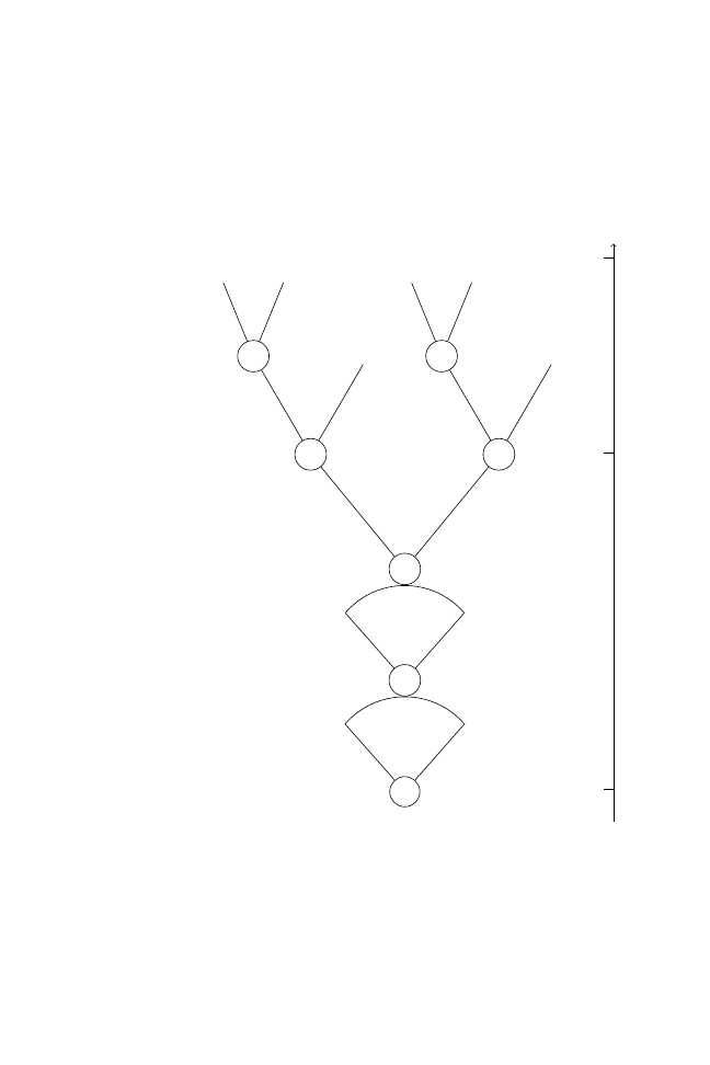
Figure

3.1:

Extensi

form

the

banking

crisis

game

between

representati

entrepreneur

(E)

and

ernment

(G)

(mo

nature

are

represented

−

open

−

open

risk

proﬁle

estment

size

deposit

withdra

bad

signal;

good

signal

bad

return;

good

return

Political Regimes, Bank Insolvency, and Closure Rules

3.1.1 Equilibrium without Government Intervention

I start by ﬁnding the equilibrium choice of

∗

in a situation in which it is

not possible to withdraw deposits at t

and there is in consequence no need

for government intervention. In this situation, all payo

ﬀs are resolved at t

and the only possible endstates are project success or failure. The probability
of reaching the good state of nature is

π, and therefore the representative

entrepreneur’s expected utility is

E(U

)

= π(R(π) − 1 − r

(S )

)

− (1 − π) w

(F)

The optimal choice for entrepreneurs is

∗

≡ argmax E(U

), subject to the

individual participation constraint R(

π) > 1 + r. This choice of π

∗

obtains

when Condition 3.1 holds:

∗

)

+ π

∗

(

∗

)

= 1 + r − w

(3.1)

moreover,

∗

is an interior solution, so the entrepreneur would not choose

∗

= 0 or π

∗

= 1. (All proofs are provided in Appendix A.1.)

Note that the entrepreneur’s chosen risk proﬁle

∗

is increasing in w and

decreasing in r (this occurs because R(

∗

)

+π

∗

(

∗

) decreases monotonically

π, while 1 + r − w is constant with respect to π). This suggests that

higher values of collateral at risk increase the choice of

∗

and, consequently,

lower the entrepreneur’s risk-taking incentives. In contrast, larger interest
rates decrease

∗

, corresponding to more risky investments.

In other words,

entrepreneurs are more willing to make riskier investments—i.e., they choose
lower

∗

—if they have higher interest payments to meet.

The bank does not make decisions in this game. Were the bank able to

set

∗

directly, it would seek to maximize

E(U

)

= π · rdD, a function that

is clearly increasing in

∗

. In other words, the bank would never choose to

make risky investments.

3.1.2 Equilibrium with a Bagehot Enforcer

Because of the absence of liquidity shocks, there is no rationale for govern-
ment intervention in the simple version of the game analyzed in the previous
section. In this section, I consider government intervention but still omit com-
plications from the inclusion of political mechanisms; thus, I simply assume

By the envelope theorem, expected utility can be seen to be decreasing in r and w.

This counterintuitive result follows from the assumption that the bank makes no proﬁts from

its lending activity. In this setup, the bank can only incur disutility from choosing

∗

< 1. In a

more realistic setup, one could divide interest payment r between bank and depositors, which

would lead to a bank’s choice of

∗

< 1.

Curbing Bailouts

that the government has a mandate to close banks at t

upon observation of s

and to leave the bank open upon observation of s

. Under these circumstances,

the government would simply loan dD to the bank at t

upon observation of

and recover this same amount at t

provided that the good state of nature

obtains. In other words, the government acts as a “no-nonsense” Bagehot
enforcer that closes banks to prevent further deterioration of balance sheets if

“things look dire,” but always leaves banks open if it receives a good signal

regardless of the size of the liquidity shock.

Knowing that she faces a Bagehot government, the entrepreneur calculates

her payo

ﬀ based on the ex ante probabilities of observing s and R. Hence, the

expected payo

ﬀ to the representative entrepreneur is

∗

Pr(R

)

(S )

+ (1 − q)(1 − π

∗

)

Pr(R

)

(F)

which reaches a maximum when the ﬁrst-order condition captured in Equa-

tion 3.2 is satisﬁed:

∗

)

+ π

∗

(

∗

)

= 1 + r − (1 − q)w

(3.2)

The entrepreneur’s expected utility is now weighted by the quality q of

signal s. Compare this equilibrium choice of

∗

to the one that obtains in the

absence of government intervention (Equation 3.1). Because 1

+ r − w ≤ 1 +

− (1 − q)w, entrepreneurs are willing to take more risk when interacting with

a Bagehot government. By being forced to forego projects upon observation
of signal s

, entrepreneurs diminish the probability of losing collateral in hard

times. In fact, the incentive to take on more risk (lower

π) increases as q → 1,

i.e., as the signal about endstates becomes more reliable. Paradoxically, a
Bagehot government with recourse to a perfect signal about future losses

would provide entrepreneurs with an incentive to choose riskier projects. In

this extreme case, the government would be acting as a de facto agent of
entrepreneurs, tying their hands and forcing them to cut potential losses early
on.

Furthermore, depositors are similarly protected. They might bear some

costs in case of bank liquidation (recall that we have assumed L

= 1 for the

sake of simplicity, but admit that liquidation might produce inconveniences

Based on assumptions about signal s, we can calculate the ex ante probabilities of observing

ﬀerent endstates:

Pr(C)

Pr(s

) Pr(R

)

+ Pr(s

) Pr(R

)

q(1

− π)

Pr(F)

Pr(s

) Pr(R

)

− q)(1 − π)

Pr(S )

Pr(s

) Pr(R

)

Political Regimes, Bank Insolvency, and Closure Rules

to depositors), but these would be minimal compared to the potential loss
−(1 − w)(y

− dy

+ d¯y) endured by depositor i if a bank that may be insolvent

were allowed to continue. Under a Bagehot enforcer with recourse to a clear

signal one would observe higher risk-taking and more forceful liquidation of
banks, but not too many costly banking crises obtaining from government
forbearance that results in eventual failure. In the extreme, as q

→ 1, a

Bagehot enforcer would be able to separate solvent from insolvent banks
perfectly. Thus, the scenario depicted in this section has close a

ﬃnity to

Bagehot’s recommendation to lend freely to solvent banks and to close down
insolvent banks, with the proviso that insolvency can be detected without
error only if the signal about future endstates is perfect (q

= 1).

3.2 Democratic Accountability, Crony Capitalism, and Systemic Risk

So far, I have considered neither the role of government as representative of
taxpayers nor the pernicious e

ﬀect of venal politicians that extract rents from

project owners in exchange for government provision of insurance in bad
times. As mentioned before, these are candidate mechanisms to explain the
role of politics in responding, and possibly contributing, to banking crises. In
short, I have not made government choices endogenous to political mecha-
nisms. I expand the basic model of Section 3.1 to consider a government that
by virtue of democratic accountability enacts the policy preferences of the
median voter (Section 3.2.1) and the possibility of crony links between gov-
ernment and entrepreneurs that might further imperil banks (Section 3.2.2).

These extensions complete the description of the political setup. I develop

comparative statics results in Section 3.3.

3.2.1 Closure Rule under Democracy

Democratic governments carry out banking policy with an eye on the electoral
arena, where they need to be mindful of the preferences of their constituents.
I argue that electoral accountability limits bailouts because it makes credible
a government’s commitment not to pump taxpayers’ money indiscriminately
into bad banks. To elaborate this argument, I assume the policy preferences
of the median voter to be most relevant under democracy. This view, which
is broadly consistent with the economic analysis of majoritarian institutions
pioneered by Downs (1957), abstracts from institutional variation within
democracies but is extremely useful to highlight di

ﬀerences across political

regimes.

As I argue in this section, implementing the policy preferences of

An inﬂuential literature studies how institutional variation determines the size of a govern-

ment’s winning coalition even across political regimes. For example, some institutions may
facilitate political survival in requiring politicians to form less-than-majoritarian coalitions in

Curbing Bailouts

the median voter makes democratic governments less likely to ﬁnance heavy
deposit withdrawals that might eventually lead to large ﬁnancial losses.

If one assumes the primacy of the median voter’s preferences in public

policy, and if these preferences reﬂect the economic positions of voters,
then the economic structure of society becomes paramount in understanding
banking policy. An essential component of bank bailouts is that taxpayers are
called to extend the life of banks from which they obtain unequal beneﬁt in
ordinary times. To see this, consider that citizens place di

ﬀerent demands on

banking services. For example, the World Bank’s database on bank outreach
reports that the median number of deposits per one thousand people was 528.9
in a sample of ﬁfty-four countries around 2001–2003, but this distribution is
strongly bimodal, with extremely low values in some countries (the minimum
is 14.5 for Madagascar). As one would suspect, the number of bank deposits
is strongly correlated with a country’s per capita GDP (r

= 0.68). These

statistics do not reﬂect the probability that any one individual will own a bank
deposit, let alone the level of variation in the size of deposits, but they convey
the basic idea that the costs of banking policy are spread among all even when
the beneﬁts of banking activity are more concentrated.

To capture di

ﬀerences in inequality I assume that individual incomes y

follow a Pareto distribution. This distribution is commonly employed in the
analysis of inequality because it reﬂects a situation in which there are many
poor individuals with low income

/assets, a smaller number of individuals

with middle income, and a very small fraction of wealthy individuals.

The

Pareto distribution is characterized by location (

μ > 0) and spread (σ ≥ 1)

parameters. The location parameter

μ is simply the value of the lowest

income in society. The spread parameter

σ—also referred to as the Pareto

index—determines relative levels of wealth between poor and rich; thus, as
σ increases, the proportion of very wealthy individuals drops, and therefore
inequality decreases. Thus, di

ﬀerent patterns of inequality obtain as these two

parameters vary. For each pattern of inequality, there are three characteristics
that we need to consider. First, I capture the level of inequality through the
Gini index g

≡ 1/(2σ−1); higher values of the Gini index (lower values of σ)

correspond to more inegalitarian societies. Second, the income of the average
voter is the expected value of the Pareto distribution, ¯y

= σμ/(σ − 1). Finally,

order to retain power (Bueno de Mesquita, Smith, Siverson and Morrow 2004).

For these ﬁgures, we can look at Mexico, where only 16% of the population had deposits in

a national bank on the eve of the banking crisis of 1995. As in many other economies, deposits
in Mexico are highly concentrated. In 1999, a minimum of 63,116 accounts (0.2%) made up
64.3% of the value of total deposits, whereas 13,520,453 accounts (43.7%) account for only
0.24% of the value of total deposits. In 1979, 68% of bank loans and credit were given to 5% of
borrowers (Maxﬁeld 1990, 103–106). See Beck, Demirg¨uc¸-Kunt and Martinez Peria (2008) for
an analysis of banking outreach around the world.

See for example Clementi and Gallegati (2005); Mitzenmacher (2003); Rodr´ıguez (2004).

Political Regimes, Bank Insolvency, and Closure Rules

the income of the median voter is simply the median of the Pareto distribution,
y

= 2

/σ

μ. Parameters g, ¯y, and y

capture the relevant distributive structure

of the economy.

With these assumptions in place, we can now consider government’s

options at t

. Contrary to the scenario of Section 3.1.2, we now consider

whether it makes sense to allow bank continuation at t

upon observation

of signal s

. This decision should be conditional on the size of deposit

withdrawals d, which is the second piece of information available to the

government. Under these circumstances, the government does not rely on
ex ante probabilities, but computes the probability of success and failure—
Pr(R

|s) and Pr(R

|s)—-premised upon observation of signal s and knowledge

of Pr(s

|R). Upon observing s

, the government should leave the bank open if

and only if

Pr(R

+ Pr(R

≥ C.

For the sake of argument, let us consider a government that perfectly rep-
resents the preferences of the median voter, which has income y

. The

government engages in forbearance if the condition in Equation 3.3 holds:

∗

− q + π

∗

Pr(R

)

r(1

− d)y

≥

− π

∗

)(1

− q)

− q + π

∗

Pr(R

)

− w)(y

− dy

+ d¯y)

(3.3)

I characterize the propensity of a government to choose forbearance by

deﬁning a closure rule. The closure rule depends on the size of the deposit

withdrawal that will impel the government to push for bank exit. Solving

for d in Equation 3.3, we ﬁnd that a democratic government will choose to
keep a bank open after observing s

if and only if d

≤ c

∗

, with c

∗

deﬁned in

Equation 3.4:

∗

≡

∗

− (1 − π

∗

)(1

− q)(1 − w)

∗

+ (1 − π

∗

)(1

− q)(1 − w)

¯y

− 1

(3.4)

Since the probability that the good state will obtain upon observing the

bad signal is nil (i.e., Pr(R

)

= 0, see Appendix A.1), the government

would never allow the bank to continue upon seeing s

. Upon observation

of s

, the government’s optimal choice is to leave the bank open for values

of the liquidity shock smaller than c

and to close it for values larger than

this cutpoint. Figure 3.2 shows the condition implied by Equation 3.4. The

As in Meltzer and Richard (1981) and Acemoglu and Robinson (2005), the distance between

the voter with average income (¯y) and the voter with median income (y

) will be crucial in

building auxiliary assumptions about the e

ﬀects of inequality on public policy.

Curbing Bailouts

Figure 3.2: Conditions under which a liquidity shortfall at t

will trigger

immediate bank closure

open under s

optimal strategy G

∗

{Open if s = s

and d

≤ c

, Close otherwise}. As

cutpoint c

shifts rightwards, the government is willing to leave the bank in

operation for a wider range of observed liquidity shortfalls.

We can read comparative statics o

ﬀ Equation 3.4. Note that c

→ 1 as

→ 1, i.e., the government is more likely to support banks under wider

ranges of liquidity shocks as its information about the likelihood of project
success at t

becomes more precise, which is only to be expected. We also

observe that cutpoint c

shifts rightwards as entrepreneurs choose lower levels

of risk—i.e., as

∗

→ 1.

This result has an intuitive explanation in that

higher values of

∗

make it more likely that R

will obtain. In turn, this

changes the distribution of signals, making it more likely that the government

will see s

—i.e., Pr(s

) Pr(R

) increases with

∗

(see footnote 12). Note

also that the cutpoint increases on values of w and r.

As mentioned before, we should also see variation in government re-

sponses to banking crises premised upon varying levels of wealth distribution
in society. We can see from the deﬁnition of c

∗

that the liquidation cut-o

ﬀ

point—the closure rule—moves leftwards as the ratio ¯y

increases. For-

mally, this result follows from signing

∂c

∗

/∂σ > 0 (see Appendix A.1). Since

the distance between median and average income-holders is much greater
under unequal than in egalitarian societies, a government’s closure rule should
be more liberal in relatively egalitarian societies. The rationale behind this
result is that as the distance between the incomes of the average and median
depositors increases, the ensuing redistribution of losses a

ﬀects the median

voter more heavily.

After solving for the government’s optimal strategy at t

, we can now

restate the entrepreneur’s decision problem at t

. Her situation is now dif-

ferent in that the good state of nature needs to obtain and the government
must allow the bank to continue if she is to get the high payo

ﬀ Π

(S ). In

other words, the entrepreneur claims the high payo

ﬀ if investments pan out

= R

), government sees s

, and the liquidity shock is smaller than the

government’s closure rule, i.e., d

≤ c

. Because entrepreneurs know the prob-

This result follows from signing

∂c

/∂π

∗

≡ (1 − w)(1 − q)/π

∗2

> 0.

Political Regimes, Bank Insolvency, and Closure Rules

ability distribution of R (after all, they choose

π) and s (Pr(s|R) is common

knowledge), they can estimate the ex ante probability of success at t

= 0,

which is Pr(R

, s

, d ≤ c

)

. Based on the assumption of independence of d

and R (i.e., liquidity shocks are uncorrelated with future states because depos-
itors do not monitor entrepreneurial investment choices) and the deﬁnition of
marginal and conditional distributions, the full joint probability Pr(R

, s, d ≤ c)

can be expressed as Pr(s

|R) Pr(R)F(c

∗

), where F(c

∗

)

≡ Pr(d ≤ c

∗

). By the

same token, the ex ante probability of failure is Pr(R

, s

, d ≤ c

After taking into account these probabilities, the entrepreneur’s ex ante

utility can be expressed as in Equation 3.5:

)

= π

∗

F(c

)

Pr(R

,d≤c

)

(S )

+ (1 − π

∗

)

− q)F(c

)

Pr(R

,d≤c

)

(F)

(3.5)

The entrepreneur’s ex ante utility is now weighted by two additional fac-

tors, the quality q of signal s and the probability distribution F(

·) of liquidity

shocks d. These weights complicate the characterization of an equilibrium
choice of

∗

. Recall that the government cannot directly observe the en-

trepreneur’s action (i.e., his choice of

∗

), but it can observe a consequence of

this action (i.e., the distribution of s is driven by R(

∗

)). In the environment

of imperfect information that I consider,

∗

changes the distribution of signals

s, and the entrepreneur must take this e

ﬀect into account when choosing her

optimal action.

As Repullo notes, it is di

ﬃcult to ﬁnd an analytical solution of a form

similar to that of Equations 3.1 or 3.2, let alone an explicit solution, because
the terms F(

·) are a non-linear function of π

∗

In Section 3.3, I resort to

computational methods that allow characterization of equilibrium choices of
π

∗

and G

∗

under di

ﬀerent combinations of exogenous parameters.

To see this, consider the expression for the partial derivative of

) with respect to

π in

Equation 3.6:

∂E

)

∂π

≡ F(c

)

π) + πR

(

π) − 1 − r + (1 − q)w

+ f (c

)

∂c

∂π

π(R(π) − 1 − r) − (1 − q)(1 − π)w

(3.6)

This expression is a complicated function of

∗

. An analytical solution to the game is easy to

ﬁnd when one factors out the terms inside the square brackets of Equation 3.5. Repullo (2005a)
proposes this simpliﬁcation, reasoning that the entrepreneur cannot manipulate the location of
cutpoint c

through his choice of

∗

, since

∗

remains unknown to the government (see Repullo

2005a, p. 56). This line of reasoning is not entirely satisfactory because

∗

ﬀects the probability

of observing signal s

Curbing Bailouts

3.2.2 Closure Rule under Crony Capitalism

Up to this point, I have developed the closure rule of a government that
merely reﬂects the policy preferences of the median voter. I now consider
a more realistic scenario where governments are willing to directly distort
the structure of entrepreneurial incentives by accepting a crony contract from
entrepreneurs. I model crony capitalism as an implicit contract in which
entrepreneurs pay per capita rent z in exchange for government support to
pay fraction

κ of collateral w in case of project failure.

The sum of all

entrepreneurial rents is Z.

As I show below, the upside of the crony contract is that it provides

entrepreneurs with an incentive to take on riskier investments, and therefore
allows the possibility of potentially higher economic growth and larger returns
to depositors. The downside of the crony contract is that, in case of failure,
the government needs to increase taxes above and beyond those needed to
ﬁnance loans at t

. This occurs because the government also needs to ﬁnance

κwD to cover the collateral of crony capitalists. A cynical view of crony
governments is that they do not care about the burden imposed on society,
and therefore are happy to pass whatever costs ensue from the crony contract
on to depositors. Under this extreme view, crony governments would never
close banks at t

, even upon observation of very large deposit withdrawals.

In a democratic regime, however, governments internalize at least partially
the cost of failure. How then would democracy change the propensity of a
crony government to engage in forbearance?

To answer this question, we reconsider the payo

ﬀs to the median voter in

ﬀerent endstates. Under S , the median voter still obtains r(1 − d)y

, but

under F she will not only lose

−(1 − w)(y

− dy

+ d¯y), but will be called

upon to pay

κw¯y as a tax to cover the entrepreneur’s collateral. Under these

circumstances, the median voter’s expected utility appears in Equation 3.7:

E(U

)

≡

∗

− q + π

∗

r(1

− d)y

−

− π

∗

)(1

− q)

− q + π

∗

− w)(y

− dy

+ d¯y) + κw¯y

(3.7)

Even in democratic regimes, we often ﬁnd close partnerships between

government o

ﬃcials and private entrepreneurs and bankers.

In line with this

At the heart of theories of crony capitalism we ﬁnd the exchange of rents for policy favors.

For example, Haslag and Pecchenino (2005) model cronyism as a government guarantee to pay
interest on loans. See also Vaugirard (2007).

This interpretation is popular in journalistic accounts and in politicized narratives of banking

crises. A good exemplar is L´opez Obrador (1999), a diatribe against the bank bailout in Mexico
that catapulted its author to political prominence.

See for example Faccio (2006).

Political Regimes, Bank Insolvency, and Closure Rules

view, I assume that politicians also include rents as part of their utility function.
I stipulate that the crony contract generates rents Z that are an increasing
function of

κ. I assume further that rents increase at a decreasing rate.

These

rents can be interpreted broadly: As economic support from entrepreneurs
that politicians can enjoy privately or spend in electoral campaigns, as ego
rents derived from close contacts with friends with money, or as future
proﬁt opportunities made possible by building extensive networks of business
contacts while in government. In the model, the government enjoys rents

whenever the bank remains open at t

and investments pan out at t

, and

obtains 0 otherwise.

Under this broad interpretation of crony rents, governments may devise a

banking policy that provides entrepreneurs with incentives to pursue riskier
investments. A government’s banking policy now comprises two interrelated
aspects, namely, a decision about the closure rule and a decision about the
extent of opportunities for cronyism. To analyze the e

ﬀect of alternative

political regimes over a government’s banking policy, we consider the ex-
pected payo

ﬀ of a government that has separable utility over crony rents and

the discounted policy preference of the median voter (Equation 3.7). The
discount weight

α captures gradations in the government’s incentive to repre-

sent the median voter. As

α → 1, which corresponds to a fully democratic

regime, government ponders the preferences of the median voter fully. The
government’s expected utility from accepting a crony deal of size

κ appears

in Equation 3.8:

)

≡

∗

− q + π

∗

αr(1 − d)y

+ Z(κ)

−

− π

∗

)(1

− q)

− q + π

∗

α(1 − w)(y

− dy

+ d¯y) + ακw¯y

(3.8)

There is no reason to consider the crony contract

κ to be an exogenous

parameter in the model. Instead, I consider

κ to be endogenously determined

by the government. Rather than adding a bargaining game over the choice
of

κ to the model, let us simply assume that the government has the chance

to reject crony deals that fail to maximize its expected utility and that there
are no commitment problems between government and entrepreneurs. Under
these circumstances, an authoritarian regime that is absolutely unresponsive
to the median voter would have no qualms admitting a crony contract setting
κ

∗

= 1 in return for Z(1). But as soon as consideration of the median

voter’s preferences weighs in on the government’s utility function, a contract
stipulating

∗

= 1 would no longer be desirable. Based on Equation 3.8, the

κ) is assumed continuous and twice-diﬀerentiable, with Z

(

κ) > 0, Z

(

κ) < 0, Z(0) = 0,

and Z

(0)

= ∞.

Curbing Bailouts

entrepreneur’s decision problem reasoning backwards from the last stage of
the game is to o

ﬀer government the value of κ that maximizes E(U

). This

value obtains when the following condition is met (see Appendix A.1):

(

κ) = α

− π

∗

− q)w¯y

(3.9)

We would like to understand how the crony contract changes under gra-

dations in the representativeness of the political regime and in levels of in-
equality and wealth in society. Consider ﬁrst how

κ changes as α approaches

1. Because Z

(

κ) is decreasing over the range of κ (see fn. 22), increases

in the right hand side of Equation 3.9 correspond to lower values of

∗

. It

follows that as

α increases, the entrepreneur oﬀers lower values of κ

∗

, i.e.,

a crony contract that is less onerous to society. Now consider parameters
σ and μ. By an identical argument, it follows that as the average income
in society increases, the size of the crony deal that entrepreneurs o

ﬀer to

government decreases. Since ¯y increases with both

μ and σ, I conclude that

higher overall income levels and more egalitarian distributions of income
reduce the propensity to engage in crony capitalism (see Appendix A.1).

The constraining e

ﬀect of democracy on banking policy extends then

to the decision to limit or expand crony networks in the banking system.
Because democracy compels politicians to consider the policy preferences
of the median voter, and because cronyism increases the potential cost of
restoring bank solvency, it follows that in democratic regimes politicians

will choose not to engage in onerous forms of crony capitalism. This may

sound altogether as an extremely rosy interpretation of the links between
democracy and cronyism. This conclusion, however, is in line with common
interpretations of the prevalence of cronyism. For example, Haber (2002b)
suggests that cronyism is a second-best solution to the fundamental dilemma
of political economy, namely, the inability of authority to commit credibly
not to expropriate wealth. Democracy is presumably a ﬁrst-best solution to
this problem, as under this political regime governments are constrained by
assemblies that represent the interests of propertied individuals and cannot
expropriate at will. In the absence of democracy, governments can credibly
commit not to expropriate the wealth of at most a few cronies only by sharing
rents with them.

To present a full picture of the changes in banking policy across political

regimes and economic situations, we ﬁnally need to consider the e

ﬀects of

cronyism, democracy, and inequality on the government’s closure rule upon

More generally, several studies have documented a negative association between democracy

(and economic development), on the one hand, and corruption, on the other (Gerring and Thacker
2004; Montinola and Jackman 2002; Treisman 2000).

Political Regimes, Bank Insolvency, and Closure Rules

observation of signal s

≤ c

∗

≡

∗

)

− (1 − π

∗

)(1

− q)

− w + κ

∗

¯y

∗

+ (1 − π

∗

)(1

− q)(1 − w)

¯y

− 1

(3.10)

We can say that democracy has a partial direct containment e

ﬀect on the

government’s closure rule: For constant levels of

κ, an increase in α shifts the

cutpoint c

leftwards, which translates into a tougher closure rule. The total

ﬀect of democracy on the government’s closure rule is more convoluted, as

is a function of the equilibrium choices of

∗

and

∗

, which are themselves

ﬀected by changes in political regime. In fact, it is not possible to sign the

net e

ﬀect of democracy on the government’s closure rule through analytical

means. To anticipate some of the results in Section 3.3, I ﬁnd that higher
values of

α lead to lower values of c

. In other words, the propensity to

forbear is lower in more democratic regimes, all else equal.

Finally, I solve for the entrepreneur’s equilibrium choice of

∗

, taking into

account the equilibrium choice of

∗

. The representative crony entrepreneur’s

expected utility appears in Equation 3.11:

)

≡ π

F(c

∗

)

π) − 1 − r − Z(κ

∗

)

− (1 − π)

− q)F(c

∗

)

− κ

∗

(3.11)

The entrepreneur thus sets

∗

to satisfy the ﬁrst order condition in Equa-

tion 3.12, subject to R(

∗

)

≥ 1 + r + Z(κ

∗

F(c

)

π) + πR

(

π) − 1 − r − Z(κ

∗

)

+ (1 − κ

∗

)(1

− q)w

= f (c

)

∂c

∂π

− κ

∗

)(1

− q)(1 − π)w − π

π) − 1 − r − Z(κ

∗

)

(3.12)

The equilibrium in this game is a choice of a strategy proﬁle (

∗

, G

∗

) from

which neither player has an incentive to deviate. Equilibria are guaranteed to

exist in this game, because the choice-sets of players are ﬁnite in the case of
government, and closed and bounded in the case of the entrepreneur. Because
of the di

ﬃculty of signing the eﬀect of α on choice parameters, I propose a

computational approach in Section 3.3 to analyze comparative statics in this
game.

I assume that the restriction R(

∗

)

≥ 1 + r + Z(κ) is not binding at π

∗

Curbing Bailouts

Table 3.4: Assumptions about functional forms and values of exogenous
variables used in the computational analysis

Function

Speciﬁc form

Param.

Values

κ)

√

0.25, 0.35, 0.45, 0.55

π)

− (π + 1)

0.5, 0.6, 0.8, 0.9

F(c)

⎧⎪⎪

⎨

⎪⎪⎩

− c

if c

∈ [0, 1]

otherwise

0.6, 0.7, 0.8, 0.9

0.04, 0.06, 0.08, 0.10

3.3 Solving for Equilibria of the Bagehot-Bailout Model

Because of the sheer di

ﬃculty of ﬁnding analytical solutions to the model, the

purpose of this section is to use computational tools to analyze the behavior
of entrepreneurs and government under alternative scenarios. The ﬁrst step to
proceed with this analysis is to choose appropriate forms for the functions that
have so far remained unspeciﬁed, namely, R(

·), F(·), and Z(·). The second

step is to consider equilibrium strategies under combinations of a manageable
set of reasonable values of exogenous parameters, in this case

σ, q, r, and

w. Recall that I characterize democratic regimes as those where

α → 1, and

authoritarian regimes as those where

α → 0. Ultimately, I seek to derive

the impact of

α on the choice of endogenous parameters in the model—risk

proﬁle

∗

, closure rule c

∗

, crony contract k

∗

, and the ex ante probability Pr(F)

of observing failure. The behavior of these four endogenous parameters is
the object of interest in this section.

Table 3.4 summarizes the values of exogenous parameters and functional

forms for R(

·), F(·), and Z(·) that I consider in this exercise. Since the results

of the analysis are dependent on the chosen functional forms and values of
exogenous parameters, it is important to consider these with care. Regarding
functional forms, I choose as simple a function as possible while still com-
plying with the assumptions of the model. Regarding exogenous parameters,
I sought reasonable values that corresponded to historical experience. For
example, the range of Gini indices spans the experience of countries such as
Denmark or Finland, with Gini scores in the neighborhood of 0.2, to Brazil
or Mexico, with Gini indices hovering around 0.55.

The chosen values

for r reﬂect the historical minima and maxima of the US prime rate over
the past ten years; di

ﬀerent choices, for example 1 or 2 points over Libor,

The values in Table 3.4 correspond to values of

σ of 2.5, 1.9, 1.6, and 1.4.

Political Regimes, Bank Insolvency, and Closure Rules

would have yielded scores in the same ballpark. The more di

ﬃcult choice

corresponds to values of w because the market value of loan collateral shifts
during ﬁnancial crises, a complication not considered here; for this parameter,
I consider a broader range from 0.6 to 0.9. The model becomes uninteresting
as q approaches 1, in which case the government is assumed to have perfect
foresight about bank net worth and acts as a ﬂawless Bagehot enforcer, so
I choose values for this parameter that are bounded away from 1. Finally, I
allow

α to take on values from 0.01 to 1, which correspond to the full range

of this parameter while avoiding undeﬁned results when

α = 0.

As I discuss the major implications of the analysis, it is inconvenient

to present graphically or numerically the equilibria that obtain under all
combinations of exogenous parameters.

Instead, I present some illustrations

in Figures 3.3 and 3.4; these ﬁgures provide a rather complete summary of
how endogenous parameters change in response to changes in political regime,
i.e., they o

ﬀer an accurate representation of the comparative statics that obtain

under other combinations of parameters. With one exception, I ﬁnd that the
relations between democracy, on the one hand, and

π, κ, and c, on the other,

are easy to characterize, as most of these are monotonically increasing or
decreasing. Where appropriate, I indicate some of the exceptions that I have
found and discuss what impact these may have on predictions.

Figure 3.3 shows the proﬁles of closure rule (c

) and risk choice (

π), the

main endogenous parameters in this analysis, under di

ﬀerent combinations

of parameters r, w, and q, and for di

ﬀerent values of the democracy weight

α. Consider the leftmost panel ﬁrst, which comprises a 4 × 3 matrix of plots.
In each column within this matrix, the clarity of signal q is held constant at
values of 0.6, 0.75, and 0.9, respectively. Within each of the twelve plots,
the values of interest rate r and collateral w are held constant at levels that
appear in a corner of the plot; these levels result from combinations of both
high and low values of these exogenous parameters. Also within each plot,
Gini indices are held constant at high and low levels of inequality (the thicker
line corresponds to a Gini of 0.55, the lighter line to a Gini of 0.25). Thus,
for example, the northwest plot in the left panel of Figure 3.3 corresponds
to the choice of closure rule c

as a function of democracy when exogenous

parameters are held constant at the following values: q

= 0.6, r = 0.06, and

= 0.7.

The easiest result to characterize is the government’s choice of closure

rule, which is monotonically decreasing on

α at all inspected combinations

of exogenous parameters (see the right panel in Figure 3.3). Note that for

One last exogenous parameter,

μ, remains ﬁxed at 10. This parameter simply shifts the scale

of results through its e

ﬀect on factor Z(κ)/y

in Equation 3.10.

The number of combinations of exogenous parameters is 4

× 10, a relatively small but still

cumbersome set of combinations.

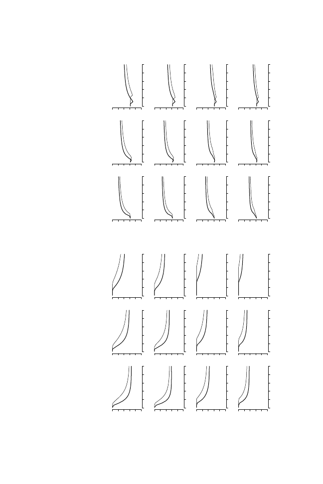
Figure

3.3:

Choice

closur

rule

)

and

risk

oﬁle

(π

∗

)

under

alternati

alues

democrac

(α

)

and

inequality

Thick

lines

correspond

higher

inequality

55),

thinner

lines

wer

inequality

.25).

The

numbers

within

the

plots

correspond

alues

and

columns

correspond

alues

equal

0.6,

0.75,

and

0.9,

respecti

ely

Closure

rule

Risk

proﬁle

Democracy weight

Closure rule

0.0

0.4

0.8

0.0

0.2

0.4

0.6

0.8

1.0

0.06

0.7

Democracy weight

Closure rule

0.0

0.4

0.8

0.0

0.2

0.4

0.6

0.8

1.0

0.06

0.7

Democracy weight

Closure rule

0.0

0.4

0.8

0.0

0.2

0.4

0.6

0.8

1.0

0.06

0.7

Democracy weight

Closure rule

0.0

0.4

0.8

0.0

0.2

0.4

0.6

0.8

1.0

0.1

0.7

Democracy weight

Closure rule

0.0

0.4

0.8

0.0

0.2

0.4

0.6

0.8

1.0

0.1

0.7

Democracy weight

Closure rule

0.0

0.4

0.8

0.0

0.2

0.4

0.6

0.8

1.0

0.1

0.7

Democracy weight

Closure rule

0.0

0.4

0.8

0.0

0.2

0.4

0.6

0.8

1.0

0.06

0.9

Democracy weight

Closure rule

0.0

0.4

0.8

0.0

0.2

0.4

0.6

0.8

1.0

0.06

0.9

Democracy weight

Closure rule

0.0

0.4

0.8

0.0

0.2

0.4

0.6

0.8

1.0

0.06

0.9

Democracy weight

Closure rule

0.0

0.4

0.8

0.0

0.2

0.4

0.6

0.8

1.0

0.1

0.9

Democracy weight

Closure rule

0.0

0.4

0.8

0.0

0.2

0.4

0.6

0.8

1.0

0.1

0.9

Democracy weight

Closure rule

0.0

0.4

0.8

0.0

0.2

0.4

0.6

0.8

1.0

0.1

0.9

Democracy weight

Equilibrium risk profile

0.0

0.4

0.8

0.0

0.2

0.4

0.6

0.8

1.0

0.06

0.7

Democracy weight

Equilibrium risk profile

0.0

0.4

0.8

0.0

0.2

0.4

0.6

0.8

1.0

0.06

0.7

Democracy weight

Equilibrium risk profile

0.0

0.4

0.8

0.0

0.2

0.4

0.6

0.8

1.0

0.06

0.7

Democracy weight

Equilibrium risk profile

0.0

0.4

0.8

0.0

0.2

0.4

0.6

0.8

1.0

0.1

0.7

Democracy weight

Equilibrium risk profile

0.0

0.4

0.8

0.0

0.2

0.4

0.6

0.8

1.0

0.1

0.7

Democracy weight

Equilibrium risk profile

0.0

0.4

0.8

0.0

0.2

0.4

0.6

0.8

1.0

0.1

0.7

Democracy weight

Equilibrium risk profile

0.0

0.4

0.8

0.0

0.2

0.4

0.6

0.8

1.0

0.06

0.9

Democracy weight

Equilibrium risk profile

0.0

0.4

0.8

0.0

0.2

0.4

0.6

0.8

1.0

0.06

0.9

Democracy weight

Equilibrium risk profile

0.0

0.4

0.8

0.0

0.2

0.4

0.6

0.8

1.0

0.06

0.9

Democracy weight

Equilibrium risk profile

0.0

0.4

0.8

0.0

0.2

0.4

0.6

0.8

1.0

0.1

0.9

Democracy weight

Equilibrium risk profile

0.0

0.4

0.8

0.0

0.2

0.4

0.6

0.8

1.0

0.1

0.9

Democracy weight

Equilibrium risk profile

0.0

0.4

0.8

0.0

0.2

0.4

0.6

0.8

1.0

0.1

0.9

Political Regimes, Bank Insolvency, and Closure Rules

very low values of

α, the optimal closure rule is 1, which means that the

government would always leave banks in operation regardless of the size of
the deposit withdrawal at t

. In contrast, lower values of c

, corresponding to

tougher closure rules, appear as

α approaches 1. As the plot reveals, closure

rules are more liberal for higher values of w and lower values of r, though
the latter e

ﬀect is minuscule. Also as expected, closure rules become more

liberal as the clarity of signal s improves (i.e., the curves representing choice
of c

shift upwards from column 1 to column 2 to column 3). Note ﬁnally that

closure rules are more liberal in more egalitarian societies. This is a direct
consequence of the mechanism assumed here, which leads governments to

weight heavily the distance between median and average taxpayers when

setting the closure rule. This e

ﬀect is less powerful as parameter α approaches

0, as under these circumstances diminished electoral accountability leads
the government to place less weight on the preferences of the median voter.

At high levels of

α, government has an incentive to internalize the policy

preferences of the median voter, which are for lower redistribution of the
burden of ﬁnancial loss. This incentive should lead democratic governments
to adopt more cautious banking policies, i.e., to avoid “kicking the can down
the road” and wind down distressed banks sooner rather than later. On the
basis of this result, I posit Proposition 1:

Proposition 1 Democracies are more likely to adopt harsher closure rules,
all else constant.

Proposition 1 ﬂows more or less directly from assumptions about the costs
of di

ﬀerent banking policies to taxpayers. After all, if taxpayers dislike

footing the bill of bank insolvency, and if governments are faithful agents of
taxpayers, they will be less likely to “wait and see” for the happy eventuality
that distressed banks will deliver good results. However, this proposition
is far from trivial. First, the strength of this result does not follow from a
government’s reaction to a banking crisis, but from government anticipation
about the potential burden of insolvency. Second, the comparative statics
portrayed in the left panel of Figure 3.3 provide an auxiliary implication,
namely, that more egalitarian societies will have more liberal closure rules

when holding levels of democracy constant. Third, Proposition 1 holds even
when we factor in the possibility that governments may want to prevent

systemic risk derived from bank failures, as I show in Section 3.3.1. Finally,
the explanatory power of the theory rests not only on this proposition, but on
two other testable implications.

The second implication follows from analysis of the risk proﬁle chosen

by entrepreneurs. The ease with which one can characterize equilibrium
choices of c

∗

is almost replicated in the analysis of

∗

in the right plot of

Figure 3.3. Here we ﬁnd that, in general,

π increases as societies become

Curbing Bailouts

more democratic (

α → 1), which means that entrepreneurs would choose

investments with lower risk. A logic of anticipation is also at play, as en-
trepreneurs have incentives to rein in their propensity to take on higher risks
once they understand that democratic regimes enact tougher closure rules.

Based on these results, I submit Proposition 2:

Proposition 2

Democracies provide lower incentives to engage in excessive

risk taking, all else constant.

The constraining e

ﬀect of democracy is also at play in the choice of crony

contract, itself a function, among others, of risk proﬁle

∗

. Across the board,

the size of the crony contract diminishes monotonically on

α, as can be

gleaned from the left plot in Figure 3.4. For low values of this parameter, lack
of democratic accountability means that the government will ﬁnd it attractive
to accept the highest possible crony contract, i.e.,

κ = 1. Furthermore, the

government’s closure rule is increasing in the size of the crony contract

(results not shown). In my theory, democracy has a direct e

ﬀect on the

choice of the closure rule through minimization of the burden of ﬁnancial
insolvency, but democracy also has an indirect e

ﬀect on the choice of closure

rule through minimization of crony contracts. In fact, the willingness of
democratic governments to accept large crony deals increases with the clarity
of signals about future states. Were this signal perfect (q

= 1), the government

would have no qualms accepting the high crony contract because it would be

able to avoid the downside risk of a bad payo

ﬀ (this eﬀect is clearly seen in

Equation 3.9). However, the incentive to take on a crony contract decreases
very fast once a certain threshold of representation is achieved. After reaching
values of

α ≈ 0.5, the choice of crony contract as a function of α continues

to decrease, though at a much lower pace. Incidentally, the choice of crony
contract is lower in more unequal societies across political regimes. This
e

ﬀect is consistent with assumptions about the preferences of the median

voter. When inequality is high, the burden of insolvency will be relatively
more onerous to the median voter. To reduce this burden, governments in
more unequal societies will choose tougher closure rules, as explained above,
but they also choose lower crony contracts (lower

∗

), which in turn increases

the equilibrium choice of

∗

Aside from these metrics, which are of direct interest and are more or less

easy to characterize, I brieﬂy consider the predictions of the model concerning

The “kinks” in the equilibrium risk proﬁle that appear in the rightmost column are the result

of two e

ﬀects. As α → 0, the equilibrium choice of κ

∗

= 1, which eliminates the negative term in

the entrepreneur’s expected utility in Equation 3.11. A similar result obtains as q

→ 1; this also

results in minimizing the size of the entrepreneur’s loss in the bad state of nature, as discussed in
Section 3.1.2.

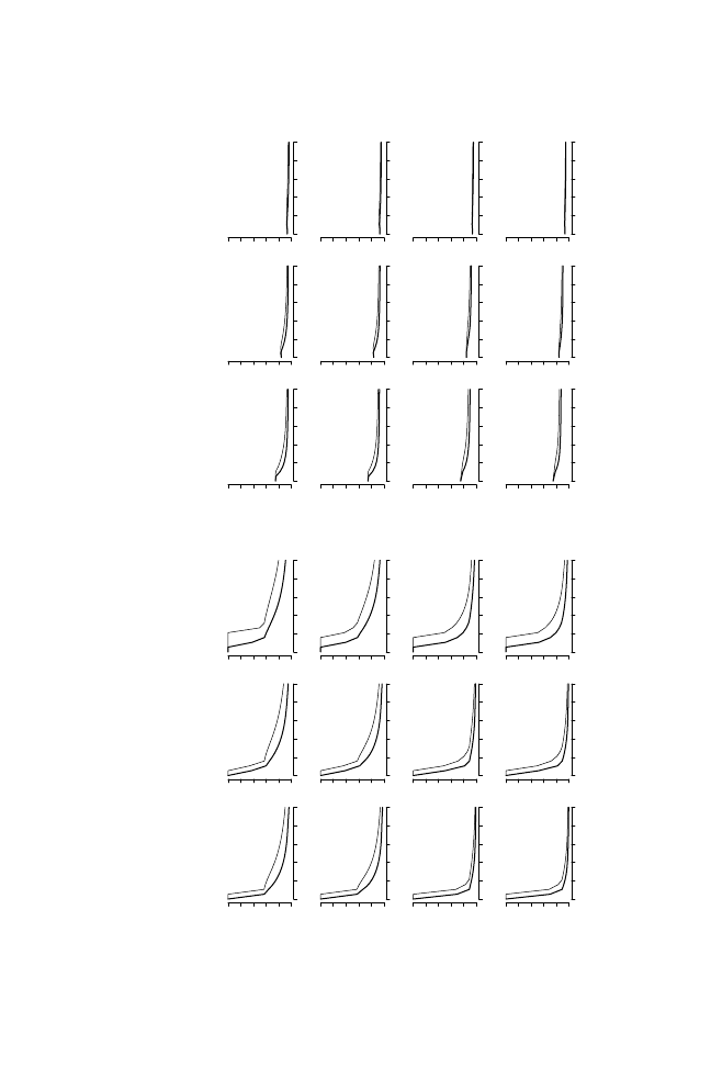
Figure

3.4:

Size

ony

contr

act

app

∗

)

and

the

ante

obability

failur

(Pr

))

under

alternati

alues

democrac

(α

)

and

inequality

each

plot,

the

thick

line

corresponds

higher

inequality

55),

the

thinner

line

wer

inequality

.25).

The

numbers

within

the

plots

correspond

alues

and

columns

correspond

alues

equal

0.6,

0.75,

and

0.9,

respecti

ely

Cron

contract

Probability

failure

Democracy weight

Size of crony contract

0.0

0.4

0.8

0.0

0.2

0.4

0.6

0.8

1.0

0.06

0.7

Democracy weight

Size of crony contract

0.0

0.4

0.8

0.0

0.2

0.4

0.6

0.8

1.0

0.06

0.7

Democracy weight

Size of crony contract

0.0

0.4

0.8

0.0

0.2

0.4

0.6

0.8

1.0

0.06

0.7

Democracy weight

Size of crony contract

0.0

0.4

0.8

0.0

0.2

0.4

0.6

0.8

1.0

0.1

0.7

Democracy weight

Size of crony contract

0.0

0.4

0.8

0.0

0.2

0.4

0.6

0.8

1.0

0.1

0.7

Democracy weight

Size of crony contract

0.0

0.4

0.8

0.0

0.2

0.4

0.6

0.8

1.0

0.1

0.7

Democracy weight

Size of crony contract

0.0

0.4

0.8

0.0

0.2

0.4

0.6

0.8

1.0

0.06

0.9

Democracy weight

Size of crony contract

0.0

0.4

0.8

0.0

0.2

0.4

0.6

0.8

1.0

0.06

0.9

Democracy weight

Size of crony contract

0.0

0.4

0.8

0.0

0.2

0.4

0.6

0.8

1.0

0.06

0.9

Democracy weight

Size of crony contract

0.0

0.4

0.8

0.0

0.2

0.4

0.6

0.8

1.0

0.1

0.9

Democracy weight

Size of crony contract

0.0

0.4

0.8

0.0

0.2

0.4

0.6

0.8

1.0

0.1

0.9

Democracy weight

Size of crony contract

0.0

0.4

0.8

0.0

0.2

0.4

0.6

0.8

1.0

0.1

0.9

Democracy weight

Probability of failure

0.0

0.4

0.8

0.0

0.2

0.4

0.6

0.8

1.0

0.06

0.7

Democracy weight

Probability of failure

0.0

0.4

0.8

0.0

0.2

0.4

0.6

0.8

1.0

0.06

0.7

Democracy weight

Probability of failure

0.0

0.4

0.8

0.0

0.2

0.4

0.6

0.8

1.0

0.06

0.7

Democracy weight

Probability of failure

0.0

0.4

0.8

0.0

0.2

0.4

0.6

0.8

1.0

0.1

0.7

Democracy weight

Probability of failure

0.0

0.4

0.8

0.0

0.2

0.4

0.6

0.8

1.0

0.1

0.7

Democracy weight

Probability of failure

0.0

0.4

0.8

0.0

0.2

0.4

0.6

0.8

1.0

0.1

0.7

Democracy weight

Probability of failure

0.0

0.4

0.8

0.0

0.2

0.4

0.6

0.8

1.0

0.06

0.9

Democracy weight

Probability of failure

0.0

0.4

0.8

0.0

0.2

0.4

0.6

0.8

1.0

0.06

0.9

Democracy weight

Probability of failure

0.0

0.4

0.8

0.0

0.2

0.4

0.6

0.8

1.0

0.06

0.9

Democracy weight

Probability of failure

0.0

0.4

0.8

0.0

0.2

0.4

0.6

0.8

1.0

0.1

0.9

Democracy weight

Probability of failure

0.0

0.4

0.8

0.0

0.2

0.4

0.6

0.8

1.0

0.1

0.9

Democracy weight

Probability of failure

0.0

0.4

0.8

0.0

0.2

0.4

0.6

0.8

1.0

0.1

0.9

Curbing Bailouts

expected ﬁnancial losses. For high values of signal q and exogenous parame-
ters w and r, the potential ﬁnancial loss under Failure is ﬂat for all values of
α (plots not shown). But as the signal loses clarity and exogenous parameters
take on lower values, the higher risk-taking propensity of entrepreneurs com-
bines with a more liberal government’s closure rule to produce higher losses
under Failure. The tendency of authoritarian regimes to yield higher losses
under Failure is consistent with evidence in Keefer (2007), who ﬁnds that
democratic regimes tend to produce lower ﬁscal costs than non-democracies
as they seek to contain banking crises.

Finally, I underscore the fact that democratic regimes limit not only the

costs of potential failure, but also the probability of failure itself. This is
shown in the right plot of Figure 3.4 where, in parallel with the discussion
about potential ﬁnancial losses, inequality seems to have no strong e

ﬀect

on the probability of failure. Note also that the e

ﬀect of democracy on the

probability of failure diminishes as the signal about future endstates becomes
clearer. In the limit, as q

→ 1, political regimes stop having an impact on

the probability of failure. To the extent that political regimes matter, my
account suggests that their e

ﬀect occurs through representation of taxpayers’

preferences in an environment of uncertainty about future payo

ﬀs. This leads

to Proposition 3:

Proposition 3 Democracies are less likely to su

ﬀer banking crises, all else

constant.

The diminished propensity of democracies to meet an endstate of Failure is not

necessarily accompanied by a larger propensity to reach Success. Admittedly,
the probability of Success is higher for democracies than for authoritarian
regimes for high values of q. For lower values of q, however, authoritarian
regimes are more likely to achieve higher rates of Success than democracy. It
is clear that democratic regimes manage to minimize the probability of Failure
by adopting tougher closure rules; these tougher rules do not necessarily
guarantee Success, but by more credibly threatening bank closures under
high realizations of deposit withdrawals they do manage to avoid very costly
instances of bank failure.

3.3.1 Preventing Systemic Risk

Even casual observation of recent banking crises suggests that governments
occasionally adopt expensive policies to restore banks to solvency, rather
than to merely see them wane. Politicians commonly appeal to the specter
of devastating ﬁnancial meltdowns as a justiﬁcation for aggressive bailouts.

To see why this rationale is important, consider that banks operate as pay-

ments clearing-houses that allow economic agents the chance to carry out

Political Regimes, Bank Insolvency, and Closure Rules

transactions with minimum e

ﬀort and that modern economies rely on banks

to manage the maturity mismatch in their income and payment streams. Thus,
businesses depend on keeping lines of credit open with banks in order to
carry out their day-to-day operations. Allowing the failure of large ﬁnancial
intermediaries entails accepting disruptions in the payments system (systemic
risk) and decreasing the amount of credit lines available to economic actors

(credit crunch). The possibility of a prolonged credit crunch and major dis-

ruption in the system of ﬁnancial intermediation is not one that governments
are willing to entertain. As a consequence, some banks and other ﬁnancial
intermediaries can be considered as simply “too big to fail.”

As pointed out by Singer (2007), defusing systemic risk is an important

rationale behind bank regulation at the domestic level. Here, I consider the
possibility of systemic risk as a rationale for avoiding failure at t

. Within the

formal setup, I model this possibility as a requirement that the bank recover
full solvency at t

. This means levying taxes to cover the bank’s full ﬁnancial

loss of

−(1 − w)D rather than simply the loss of the government loan at t

. By

restoring bank solvency, depositors are assured of recovering their remaining
deposits at t

. This means that their ﬁnal payo

ﬀ under failure would be

− (1 − w)¯y, for a total taxation loss to depositor i of −(1 − w)¯y (i.e., there is

no direct deposit loss).

This policy choice corresponds to a bailout in the

sense that the full burden of ﬁnancial insolvency is passed on to taxpayers.

As I explain in Chapter 4, the bank itself may merge into a larger entity or be

nationalized, but the characteristic feature of “too big to fail” interventions
is that a huge portion of the ﬁnancial burden of bank insolvency becomes a
government liability that is ultimately backed by the taxpayer.

Within the logic developed in this chapter, a bank that is big enough to

threaten systemic risk would invite a di

ﬀerent type of reaction. In particular,

the government’s decision problem is to leave the bank open upon observation
of the “good” signal s

if Inequality 3.13 holds:

∗

− q + π

∗

αr(1 − d)y

+ Z(κ)

≥

− π

∗

)(1

− q)

− q + π

∗

α(1 − w)¯y + ακw¯y

(3.13)

Again, we can solve Inequality 3.13 in terms of d to ﬁnd the government’s

On the hazards posed by the failure of large banks, see Stern and Feldman (2004). A variety

of “optimal bailout” arguments rationalize support of distressed banks that are not necessarily
too big to fail; see for example Aghion, Bolton and Fries (1999); Cordella and Levy-Yeyati
(1999); Gorton and Huang (2004).

Because y

− dy

+ d¯y < ¯y, the median voter suﬀers lower loss when the bank is not entirely

bailed out. The implicit assumption is that the failure of a bank that threatens systemic risk

would be so costly that the median voter still prefers a bailout.

Curbing Bailouts

closure rule c

under the threat of systemic risk:

≤ c

∗

≡

∗

)

− (1 − π

∗

)(1

− q) (1 − w + κ

∗

¯y

∗

(3.14)

These changes in the government closure rule under systemic risk also

have an impact on the entrepreneur’s utility and therefore on her choice of
π

∗

Consequently, analytical comparison of rules c

and c

is rendered di

ﬃ-

cult because of the indirect e

ﬀects of α on c

and c

through

κ and π. I thus

resort to the same kind of computational analysis performed in Section 3.3.
Figure 3.5 provides a summary comparison of c

∗

and c

∗

(Equations 3.10

and 3.14) under the same set of circumstances explored in Figures 3.3 and 3.4.
Rather than directly displaying the behavior of di

ﬀerent endogenous param-

eters under alternative combinations of exogenous variables, the plots in
Figure 3.5 display the values of closure rule, risk proﬁle, crony contract, and
probability of failure conditional on varying democracy weights but averaged
across all combinations of exogenous variables. We can read these plots as
expectations about the values that endogenous parameters take conditional
on political regime.

The most relevant feature revealed by these plots is that the e

ﬀect of

democracy is not altered substantially; compared to non-democratic regimes,
democracies still exhibit tougher closure rules, lower risk-taking, and lower
probability of failure. In other words, Propositions 1 to 3 hold whether
one considers the possibility of systemic risk—banks that are too big to
fail—or the more limited intervention in which only the fraction of ﬁnancial
loss that corresponds to government support at t

is socialized. Within a

given political regime, banks that threaten to irreparably a

ﬀect the system of

ﬁnancial intermediation beneﬁt from more generous closure rules (Figure 3.5,
Plot a) and are likely to o

ﬀer higher crony contracts to the government (Plot

c). Be this as it may, this kind of bank is slightly less prone to take on risk,
as suggested by the higher value of

π in Plot b. In the end, the combination

of these factors leaves banks with and without systemic risk potential about
equally likely to fail on average. This is especially true in countries with
middling to high democracy weights (Plot d).

3.4 Toward a Strategy of Empirical Validation

I submit that democracies have an advantage over authoritarian regimes in the
realm of banking policy, an advantage that stems from the nexus of electoral

In contrast with Equation 3.5, the entrepreneur’s utility is

F(c

∗

)

(S )

− (1 −

π)

− q)F(c

∗

)

(F).

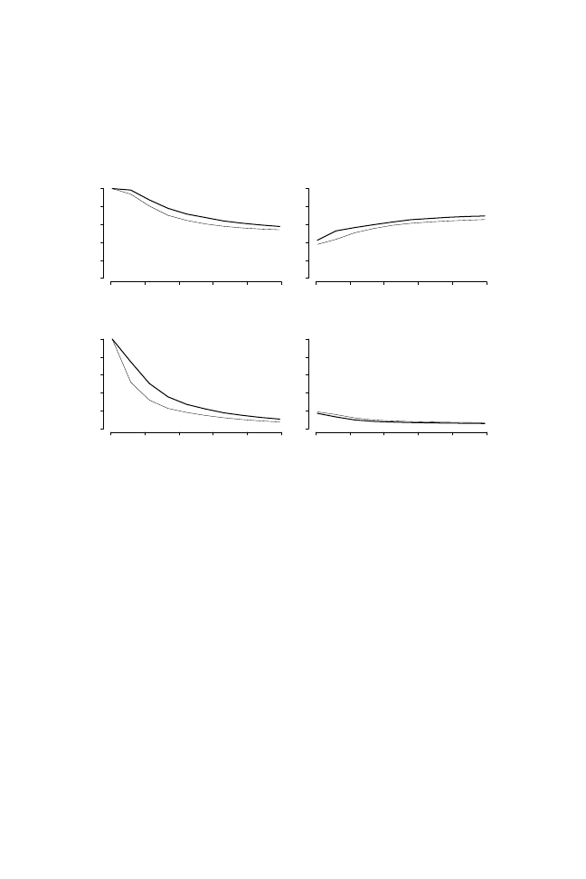
Political Regimes, Bank Insolvency, and Closure Rules

Figure 3.5: Average values of closure rule (c

), risk proﬁle (

π), crony contract

(

κ), and probability of failure (Pr(F)) conditional on democracy (α) and

systemic risk (thicker lines correspond to a bank that threatens systemic risk)

(a) Closure rule

(b) Risk proﬁle

Democracy weight

Closure rule

.00

.20

.40

.60

.81

0.0

0.2

0.4

0.6

0.8

1.0

Democracy weight

Risk profile

.00

.20

.40

.60

.81

0.0

0.2

0.4

0.6

0.8

1.0

(d) Probability of failure

Democracy weight

Crony contract

.00

.20

.40

.60

.81

0.0

0.2

0.4

0.6

0.8

1.0

Democracy weight

Probability of failure

.00

.20

.40

.60

.81

0.0

0.2

0.4

0.6

0.8

1.0

accountability. The fear of electoral retribution in democratic regimes means
that politicians are not able to downplay entirely the policy preferences of
citizens for avoiding extreme costs in the face of breakdown of the system
of ﬁnancial intermediation. In my argument, electoral accountability keeps
politicians on their toes, forcing them not only to minimize public outlays in
responding to banking crises, but also intervening forcefully and early on to
avoid the multiplication of costs from keeping heavily distressed banks alive.

The e

ﬀects of electoral accountability ﬁlter through a government’s banking

policy to the investment decisions of entrepreneurs. Entrepreneurs anticipate
that aggressive risks increase the chances of early and forceful government
intervention, which might deprive them of the possibility of seeing their in-
vestments to fruition. These alleged e

ﬀects of democracy on various banking

policy aspects are summarized in Propositions 1, 2, and 3. In general, demo-
cratic regimes should be associated with smaller crony contracts, tougher
closure rules, and lower incentives for risk-taking. Furthermore, democratic
regimes should also be associated with lower probabilities of observing costly
failures.

My argument does not imply that democratic regimes will never engage

Curbing Bailouts

in bank bailouts, let alone su

ﬀer from crippling banking crises. Aside from

the most recent spate of bank failures and bank bailouts associated with the
US subprime mortgage crisis, politicians in democratic regimes have been
called upon multiple times to contain the damage caused by insolvency of
ﬁnancial intermediaries. In the model analyzed in this chapter, banking crises
and the choice to prevent ﬁnancial meltdown by forcing taxpayers to carry the
full burden of insolvency occur because of uncertainty about the future state
of the economy. In the absence of uncertainty about future entrepreneurial
payo

ﬀs, governments would be perfectly able to discern a bank’s ﬁnancial

status down the line and would intervene early on to minimize the costs of
closure. However, governments make decisions that may prove wrong in an
environment of uncertainty about future payo

ﬀs. The most costly decision is

to leave open a bank that eventually proves to be insolvent. In this situation,
governments will be stuck with the burden of ﬁnancial loss, a burden that will
in one way or another be carried by taxpayers.

Be this as it may, I do expect the banking policies of democratic regimes

to be di

ﬀerent on average than those of non-democratic regimes. In the re-

mainder of the book, I will present the case for empirical estimation of this
democratic e

ﬀect. Because I rely on observational data, presenting the case

for a causal interpretation of a democratic e

ﬀect on banking policy requires

care in setting up empirical models. In fact, I will return in future chapters to
some of the auxiliary implications of the argument developed here to guard
against potential pitfalls in a strategy of empirical veriﬁcation. For example,
the analysis presented in this chapter suggests that levels of economic inequal-
ity exert important e

ﬀects on banking policy. At the same time, we know from

a well-established literature in political economy that economic inequality is
an important determinant of democratic consolidation.

Consequently, eco-

nomic inequality is theoretically related to both banking policy and political
regimes, and shoud be controlled for in any attempt to estimate the e

ﬀect of

democracy on banking policy. This is not necessarily the case of cronyism.

Though I expect an important degree of association between political regime

and cronyism, on the one hand, and cronyism and bailout propensities, on the
other, I also expect crony contracts to be endogenous to political regime. In
this sense, cronyism should be seen as a post-treatment variable that should
not be controlled for in models of political regime e

ﬀects. In Chapters 5 and 6,

I look at government bailout propensities under democratic and authoritarian
political regimes. These propensities are the empirical correlate of closure
rules in this chapter. In Chapter 7, I consider indicators of the risk of failure
and aggregate net worth of banking systems, which I construe as empirical
proxies of probability of failure and risk-taking proﬁles. Before embarking

See for example Acemoglu and Robinson (2005); Boix (2003); Moore (1966).

Political Regimes, Bank Insolvency, and Closure Rules

on empirical tests of the validity of Propositions 1 through 3, I consider the
policy responses of Argentina (a democratic regime) and Mexico (a semi-
authoritarian regime) to the Tequila crisis and associated bank failures of the
mid-1990s. Chapter 4 bridges the gap between the abstract representation of
policy actions as parameters in a model and the nitty-gritty details of actual
policy-making, and shows that patterns of bank survival in these countries are
broadly consistent with expectations derived from my account of the banking
policy consequences of political regimes.

Argentina and Mexico:

A Closer Look at Bank Bailouts

Models are caricatures of reality that isolate a small number of factors pre-
sumed relevant in understanding complex phenomena. Contrary to the sim-
pliﬁed portrait of crisis resolution developed in Chapter 3, the day-to-day
management of banking crises involves a variety of decisions regarding which
banks to close, how to promote recapitalization of the banking system, how
to empower banking agencies to deal with problem banks, and how much
autonomy to grant to these agencies, among others. I claim that we can look
at these policy actions as indicators of the underlying bailout propensities of
governments. As suggested in previous chapters, I see these propensities as
falling between Bagehot and Bailout ideal-types and consider that policies
close to Bailout shift a larger share of the burden of ﬁnancial insolvency to
taxpayers.

In this chapter, I review government responses to the Tequila banking

crises in Argentina and Mexico. The selection of cases is driven by the fact
that these countries were similar in respects presumed relevant by the theory
in Chapter 3—both were middle-income economies with unequal patterns
of economic opportunity—but di

ﬀered in one crucial respect: Mexico was

still in 1994–1995 a semi-authoritarian regime (admittedly, one in the process
of transiting towards open electoral contestation), whereas Argentina was a
democratic regime (though one with a chequered political history punctuated
by gruesome dictatorial interludes and with remaining authoritarian enclaves).

As suggested by the theoretical argument, the set of policies carried out by
Argentine decision-makers to address banking sector problems during the
Tequila crisis exemplify a Bagehot response, whereas the Mexican govern-

ment response approximates the Bailout model. Ideally, one would trace
di

ﬀerences in electoral accountability through the thought processes and po-

Argentina and Mexico: A Closer Look at Bank Bailouts

litical calculations of incumbent politicians all the way to variations in policy
implementation. However, few politicians in non-democratic regimes are
prone to admit publicly that they remain unmoved by the plight of taxpayers;
to the contrary, like their counterparts in democratic regimes, these politicians
are quick to argue that their policies safeguard the interests of all.

Thus, I do not provide in this chapter the “smoking gun” of politicians

in Argentina that tremble thinking about the wrath of the Argentine voter
and thus make haste in striking down distressed ﬁnancial intermediaries,
nor politicians in Mexico laughing o

ﬀ the ineﬀectual threat of electoral

accountability before extending a helping hand to insolvent banks. This
chapter o

ﬀers instead a closer look at how speciﬁc policies relate to the

Bagehot-Bailout construct of Chapter 1. The chapter shows that though these
governments lacked tools that were needed to confront a systemic banking
crisis, they both succeeded in altering the rules and framework of supervision
and regulation in order to counter liquidity and solvency problems in the
banking sector. As a result of these changes, Argentine policy-makers were
able to minimize taxpayer expenses, whereas the Mexican response was
overtly generous to banks and therefore onerous to taxpayers.

Finally, the chapter inspects the process of resolution of individual banks

in these countries for important clues about political motivation. I focus
on bank-level information as I seek to understand the determinants of the
length of bank survival. A government closer to the Bagehot ideal-type would
seek to arrange for the exit of highly distressed banks and would do so in as
short a time as possible, whereas a Bailout government would lengthen the
survival times of distressed banks and would not necessarily base its decisions
about bank exit on the ﬁnancial status of banks. Rather than indulging in an
excessively detailed account of bank restructuring policies, my purpose is
to provide a broad outline of how the Argentine and Mexican governments
faced problems of liquidity and insolvency in the banking sector.

The chapter is organized as follows. Section 4.1 considers actual policy-

implementation in Argentina and Mexico along the ﬁve issue-areas identiﬁed
in Chapter 2. The main evidence regarding the di

ﬀerent bailout proclivities

of these governments comes from empirical analysis of the Argentine and
Mexican processes of bank exit. Section 4.2 shows not only that the exit
process of Argentine banks was more rapid, but also that it remained close to
the Bagehot ideal-type by eliminating weaker banks. In Mexico, in contrast,
ﬁnancial indicators are not particularly good predictors of bank survival.
Finally, I discuss in Section 4.3 some of the reasons why a paired comparison
of these two countries is still insu

ﬃcient to arrive at inferences about the

ﬀects of political regimes on banking policy. This discussion paves the way

for a broader analysis in the rest of the book.

Curbing Bailouts

4.1 Argentina and Mexico in Comparative Perspective

In this section, I summarize the policy actions of the Argentine and Mexican
governments with regard to the ﬁrst four arenas described in Chapter 2:
liquidity support, liability resolution, asset resolution, and bank capitalization.

These cases di

ﬀer in their political regimes but are otherwise similar in factors

such as economic inequality and level of development. Be this as it may, I
do not want to overplay the similarities, as it is di

ﬃcult to see these cases as

“perfect matches” in all but one dimension. To wit, other di

ﬀerences limit my

ability to extract conclusions about the e

ﬀect of political regimes on bank

bailouts from this paired comparison. Most importantly, the Argentine and
Mexican banking sectors were di

ﬀerent in some respects in the run-up to the

Tequila crisis.

Historically, bank ownership in Latin America has been highly concen-

trated, and incentives for safe banking practices have not always been in
place.

In the 1990s, after the ﬁrst e

ﬀorts to liberalize the banking sector, the

market share of the ﬁve biggest banks amounted to 71% in Mexico and 40%
in Argentina, compared to 10–30% in developed economies.

The Mexican

system included 23 private banks (17 banks were reprivatized in 1991–1992
and six more were chartered afterwards), eight public development banks
traditionally laden with bad portfolios, and a couple of foreign banks that
carried out “second ﬂoor” operations (foreign banks were not allowed in
retail banking). Mexican commercial banks had been nationalized in 1982
and remained public until 1991, at which time they were auctioned to private
investors. The rapid sequence of bank auctions in 1991–1992 replenished
government co

ﬀers, but left the new private banks severely undercapital-

ized. Indeed, the average bid-to-book-value ratio for seventeen reprivatized
banks was a rather high 3.08 (Sol´ıs 1999, 46).

Furthermore, prudential bank

regulation after privatization remained inadequate.

The Argentine banking system was certainly more competitive, with 73

domestic private banks (which held about 38% of all assets in the banking
system), 31 foreign banks, 30 provincial banks, and 34 mutual or co-operative

De Krivoy (1996, 23).

The Economist, April 12, 1997, p. 36.

On the nationalization see Maxﬁeld (1990) and Elizondo (2001). The process of privatization

is told by its main architect in Ortiz Mart´ınez (1994). Changes to the Ley de Grupos Financieros
in 1990 and 1991 allowed a system of universal banking in which banks could participate in all
ﬁnancial markets (insurance, factoring, retail banking, investment banking, etc.). Passive interest
rates and mandatory credit channeling were also eliminated, as were all reserve requirements for
commercial banks.

For example, banks presented their balances based on di

ﬀerent accounting principles. Indeed,

one condition for the US-IMF sponsored bailout of the Mexican treasury was that banks adopted
Generally-Accepted Accounting Practices (Rubio 1998, 64).

Argentina and Mexico: A Closer Look at Bank Bailouts

banks with small market share (about 6% of all assets). Despite the vagaries of

Argentine ﬁnancial history, the set of regulatory reforms that accompanied the

Convertibility law of 1991 had created a small but relatively e

ﬃcient banking

system. As I explain below, the Convertibility law turned the Banco Central
de la Rep´ublica Argentina (BCRA) into little more than a currency board,

with limited ability to play the role of lender of last resort to the banking

system. Perhaps because of this constraint, Argentine banks were much better
capitalized than Mexican banks on the eve of the crisis; in 1994, the average
capital-asset ratio was 14.66%, much higher than the 8% recommended by
the 1988 Basel Accord, while deposits amounted to 18% of GDP. Throughout
the 1990s, the Argentine authorities invested in building a state-of-the-art
system of prudential supervision of bank activity (Calomiris 1997).

The Mexican banking crisis started in earnest in December 1994, when the

government announced that it would no longer sustain the o

ﬃcial peso-dollar

exchange rate. The hike in interest rates that followed currency devaluation
forced bank debtors into arrears: In the ﬁrst quarter of 1995, the inter-bank
interest rate rose from 34.4% to 109.7%. Currency depreciation also increased
the value of dollar-denominated liabilities in bank balance sheets. In short,
economic agents were caught overtly exposed to interest and foreign exchange
risks (see Mishkin 1996). However, the deterioration of loan portfolios that
led to generalized bank solvency had started well before December 1994.
Indeed, the Mexican bank crisis had been brewing for at least two years
as non-performing loans accumulated in bank ledgers. After privatization,
Mexican banks had aggressively expanded credit to the private sector. This
credit expansion was not pernicious per se; to the contrary, increased credit
availability was one of the purposes behind bank privatization and ﬁnancial
deregulation. Nor was credit expansion surprising, given that in the era of
nationalization banks were constrained to serve ﬁrst the ﬁnancial needs of the
government. Two unforeseen circumstances, however, made credit expansion
suspect. First, credit continued to be expensive and spreads between lending
and borrowing interest rates remained rather high following privatization.
Second, credit increased at the expense of asset quality, which plunged when
a speculative bubble in real estate and stock markets burst; when asset prices
dropped, strategic defaults became more common.

As a result, the o

ﬃcial—

probably underestimated—proportion of non-performing loans to total loan
portfolio in Mexico expanded from 0.99% in 1988 to 9.02% in the months
prior to the peso devaluation to 18.65% after the crash in 1995.

According to an o

ﬃcial account of the crisis, the government entertained

three possible strategies to deal with bank insolvency (Secretar´ıa de Hacienda

Strategic default occurs when a debtor with paying capacity is better o

ﬀ foregoing collateral

than continuing interest payments—i.e., when the unpaid portion of a loan is worth more than
collateral.

Curbing Bailouts

y Cr´edito P´ublico 1998). First, do nothing, which would have meant the de
facto bankruptcy of the banking system, with generalized bank runs and a
scramble by banks to cash assets and obtain expensive ﬁnancing, if any, in
international capital markets. The consequences of this choice would have
been even higher interest rates and a more pronounced depreciation of the
peso, both leading to a harsher economic recession. This would have cor-
responded to the Market extreme of Chapter 1. Second, (re)nationalize the
banking system, an extremely costly option as the government would have
had to recapitalize banks on its own, would have been subject to political
pressures impairing asset recovery, and would have had to compensate ex-
propriated bankers. In short, the second strategy would have implied larger
involvement of taxpayers in sharing the losses derived from bank insolvency.
The third possibility, which was eventually adopted, was to design a variety
of programs to address liquidity and solvency concerns piecemeal. Over the
following year, as the extent of bank distress became widely recognized, the
Mexican government launched a number of programs that aimed to capitalize
banks, reschedule payments for bank debtors, and restructure banks’ bad loan
portfolios. These actions required the coordinated e

ﬀort of the Secretar´ıa

de Hacienda y Cr´edito P´ublico (SHCP), Banco de M´exico (Banxico), and
the Comisi´on Nacional Bancaria y de Valores (CNBV), Mexico’s bank su-
pervisory agency. Transfers to banks were channeled through the depositor
insurance fund, the Fondo Bancario de Protecci´on al Ahorro (Fobaproa).

The Argentine bank crisis can also be precisely dated: The crisis started

with a deposit run on December 20, 1994, following the devaluation of the

Mexican peso, and was ﬁnally halted in May 1995, after presidential elections
returned Carlos S. Menem to a second term in o

ﬃce.

Government action to

stop the crisis was not immediately forthcoming, and from several accounts it
seems to have been insu

ﬃcient when it ﬁnally arrived a couple of weeks into

the crisis. As a matter of fact, the banking system improvised a liquidity safety
net to stall the deposit run, which was coordinated by the Banco de la Naci´on

Argentina (BNA), the largest public bank in the country (Fern´andez 1995).
When the deposit run did not immediately abate, the government reacted

by reducing bank reserve requirements, i.e., by allowing banks to cash non-
remunerated bank reserves (encajes) at the BCRA.

Further reductions were

granted throughout January, as encajes fell from 43%, 3%, and 1% before

For accounts of day-to-day aspects of the crisis, see Arnaudo (1996); Banco Central de la

Rep´ublica Argentina (1995); D’Amato, Grubisic and Powell (1997); Di Bella and Ciocchini
(1995); Fern´andez (1995); Rozenwurcel and Bleger (1997).

Encajes constitute the fraction of every dollar in a deposit account that banks are forced to

immobilize, unremunerated, at the Central Bank. In Argentina, these reserves served no monetary
purpose—i.e., they were not meant to reduce the e

ﬀect of the money multiplier mechanism—but

worked as implicit liquidity insurance.

Argentina and Mexico: A Closer Look at Bank Bailouts

the crisis—for sight deposits, short-term certiﬁcates of deposit (CDs), and
medium-term—to 30%, 1%, and 0% by the end of January 1995 (Fern´andez

1995, 1). Though this action at once freed over 3 billion dollars that were

used to pay depositors that ﬂed the system, the amount was not enough to
ease the bank run. The December run re-started on February 28 after the
Ministry of the Economy announced a “light” ﬁscal program to alleviate
solvency problems in the banking sector. The limited nature of this package
suggests that ﬁnancial authorities miscalculated the extent of bank insolvency,
and considered that minimal intervention would su

ﬃce at least until the end

of the presidential electoral campaign.

It was only after this limited package

failed to stem the deposit run that Argentine authorities decided to combat
insolvency in earnest. By the time the deposit run was ﬁnally stopped ﬁve
months into the crisis, deposits in the Argentine ﬁnancial system had dropped
by $8.8 billion, approximately 19% of total deposits.

After this brief account of the genesis of the Tequila crises, I now turn to

the di

ﬀerent measures that the Argentine and Mexican governments enacted

to contain them. I start with a description of how central banks and executive
agencies tackled the functions of lender of last resort, asset management, and
bank recapitalization.

4.1.1 Liquidity Support

One basic di

ﬀerence between these two countries was the institutional setup

within which they conducted monetary policy. Reforms to the charter of the

Mexican central bank in 1993 had provided Banxico with relative political
autonomy with respect to the executive.

Monetary policy was therefore

in the hands of a relatively autonomous board with a primary mandate to
preserve low inﬂation in a semi-ﬁxed exchange rate regime, as well as the
subsidiary expectation of acting as lender of last resort.

Argentina, instead, had renounced to sovereign monetary policy in an

ﬀort to preserve a ﬁxed exchange rate regime. The Organic Charter of the

BCRA, approved in 1992, had rea

ﬃrmed BCRA’s responsibility for over-

sight and guidance of the ﬁnancial system—the banking regulatory agency,
the Superintendencia de Entidades Financieras (SEF), was formally part
of the BCRA—but the BCRA was under obligation at all times to keep

According to Sturzenegger, “Cavallo [Minister of Economy] never thought that there was a

risk of a systemic run, and calculated that he could keep going until May 14, election day, with
only very light measures” (Fern´andez 1996, 79, my translation). This interpretation is endorsed
by the Asociaci´on de Bancos de Argentina (AdeBA) (see Ribas 1998).

Among the institutional innovations that made political autonomy possible, the new charter

established non-overlapping tenure of board members and the executive and provided ﬁxed terms
for Banxico board members.

Curbing Bailouts

enough reserves to support the technical convertibility ratio.

Thus, the

1991 Convertibility Law in essence required Argentina’s central bank to turn

into a currency board forced to back pesos in the domestic economy with an
equivalent amount of US dollars in its reserves. In principle, BCRA could
perform only very limited last-resort lending functions, whereas Banxico
had more latitude in carrying out these functions. The law of Convertibility
made policy-makers think that the BCRA could safely eschew instruments to
combat systemic bank crises, for these would never occur within a framework
of monetary stability. The Tequila crisis proved these expectations wrong,
and the government had to retool the central bank hastily to confront the
crisis (Rozenwurcel and Bleger 1997). As I try to make clear in the following
paragraphs, the Argentine government managed to partially free the BCRA
from the fetters of Convertibility so that it could participate in managing the
banking crisis.

Upon announcement of the peso devaluation in December 1994, Banxico

joined negotiations with the International Monetary Fund, the United States,
Canada, and the Bank of International Settlements for a set of emergency
loans amounting to $53 billion.

These resources allowed Banxico to in-

crease its lending tenfold to commercial banks in an e

ﬀort to assuage liquidity

concerns. Indeed, Mexican banks faced short-term dollar payments that had
become more di

ﬃcult to fulﬁll after the devaluation. Over the ﬁrst quarter

of 1995, the Central Bank injected $3.9 billion into sixteen domestic banks,

which were able to repay these loans within six months. Prior to privati-

zation of Mexican banks, Banxico had mandated that all banks deposited
encajes in its vaults—a proportion of each deposit that could be employed
to relieve liquidity shocks—but this practice had been eliminated in 1991.
Consequently, aside from direct help from Banxico’s discount window, the
Mexican government’s ﬁrst regulatory measure after the crisis was to force
banks to set aside loan loss provisions equal to 60% of past-due loans or 4%
of total bank credits. These regulatory measures strengthened the ability of
banks to face the immediate deterioration of their loan portfolios, but left
banks severely undercapitalized.

Banxico’s charter had equipped the central bank with tools to act as lender

of last resort, and the emergency rescue package negotiated with international
lenders provided it with enough liquidity to help banks confront the currency
shock. Furthermore, Mexico had at the time a universal system of depositor
insurance that in principle limited the potential for deposit runs. Eventually,

The main legal dispositions are included in Law 24.144, passed by Congress on September

23, 1992. This framework was slightly modiﬁed by decrees 1860

/92 and 1887/92.

Unless otherwise noted, all amounts are in current US dollars.

This section is based on Gavito and Silva (1996); Murillo (2001); Navarrete (2000); Sol´ıs

(1999).

Argentina and Mexico: A Closer Look at Bank Bailouts

the Zedillo administration sought to secure even greater autonomy for the
central bank, along with a stake in supervising the banking sector. These
reforms, however, were passed in 1998; they were informed by the experience
of the banking crisis, but were not meant to re-tool Banxico to face the crisis.

In contrast, the Argentine executive decreed measures to broaden the

BCRA’s margin of action to combat the banking crisis in what became known
as the Easter package (Law 24.485, promulgated by decree 538

/95 on April

5, 1995). Prior to these measures, the BCRA’s Organic Charter included
provisions for limited last resort lending subject to the external convertibility
constraint. Thus, BCRA loans could not exceed 30 days and could not be
larger than the requesting bank’s capital. Additionally, banks were mandated
to keep reserves (encajes) at the central bank (3% for certiﬁcates of deposit,

43% for sight deposits), which they could access to confront localized deposit

runs. Also in contrast with Mexico, the ﬁxed exchange rate in Argentina was
not immediately threatened thanks to the Convertibility law, but the ability
of banks to cash sight deposits was imperiled by the extent and speed of the
deposit run and by legal limits placed on last-resort lending by the central
bank. To counter liquidity problems, the Easter reforms extended repayment
schedules for banks accessing the central bank’s discount window (from 30
to 90 days) and increased the maximum amounts that the central bank could
lend (in any case, the requirement that discount loans should be guaranteed

with good collateral remained). Concurrently, the government announced

resumption of Argentina’s access to the IMF’s extended fund facility (2.4
billion dollars), which had expired the previous year, and reduced the reserve
requirement that forced banks to keep money in the central bank (Fern´andez

1995; Rozenwurcel and Bleger 1997).

4.1.2 Liability Resolution

As was the case with the institutional conﬁguration of the monetary author-

ity, Argentina and Mexico di

ﬀered with regard to the extent of their safety

nets for depositors. Undoubtedly, their di

ﬀerent arrangements regarding

depositor insurance reﬂected historical experience with previous banking
crises. Argentina, to a greater extent than Mexico, had experienced previ-
ous banking crises in which the agency in charge of deposit insurance had
extended coverage to all depositors, producing heavy losses that were pub-
licly funded (Bali˜no 1990; Piekarz 1981). In consequence, the architects of
the post-Convertibility ﬁnancial system abolished deposit insurance (Braes-

Rozenwurcel and Bleger (1997) provide the following breakdown of resources to stop the

deposit run: $4.1 bn. were freed from reduction in central bank reserve requirements (reservas),
$2.2 bn. from direct BCRA assistance (pases and redescuentos), and $2.5 bn. from commercial
banks’ reluctance to extend new loans.

Curbing Bailouts

sas and Naughton 1997). The Argentine ﬁnancial system went practically
overnight from enjoying a generous safety net to having none, and indeed
some commentators claim that the absence of a safety net for depositors
contributed to the propagation of the Tequila crisis in Argentina (Ribas 1998).
Mexican depositors, in contrast, enjoyed the explicit backing of Fobaproa;
the generous protection it a

ﬀorded depositors was eventually seen as one of

the factors producing moral hazard in the Mexican banking system. Against
this institutional di

ﬀerence, it is notable that both governments restructured

deposit insurance protection radically as they sought to contain solvency and
liquidity problems.

In Argentina, the central bank charter explicitly stipulated that the BCRA

could not grant guarantees “that directly or indirectly, implicitly or explic-
itly, covered liabilities of ﬁnancial entities, including those originating from
deposit-taking” (Article 19, Paragraph K, my translation). Small depositors

were given seniority status in the event of bank closure, and there was legal

basis to use encajes (bank reserves in the central bank) to liquidate their
deposits.

In consequence, one would think that instances of bank closure

during the Tequila crisis should have produced large losses to depositors, but
in fact only a handful of individuals lost money.

The reason why depositors

failed to take large losses was the creation of system of asset resolution that

Argentine regulators perfected during the Tequila crisis. As mentioned before,

it is di

ﬃcult in practice to separate asset and liability resolution. In the case

at hand, the asset resolution mechanism that prevented depositor losses was
managed by Seguro de Dep´ositos, S.A. (Sedesa), a deposit insurance agency
created in April to manage the Fondo de Garant´ıa de Dep´ositos (Fogade).

Stakeholders of Sedesa included the Central Bank and all commercial banks
in proportion to the size of their deposits. In calculating each bank’s participa-
tion in the Fogade, Argentine regulators embraced best practice by requiring
payments that were a function of the bank’s risk level. Thus, payments to
the fund were between 0.015 and 0.06% of all peso- and dollar-denominated
deposits. Participation in the fund became mandatory for all banks, domestic
or foreign, operating in Argentina.

During the crisis, Sedesa was steered by an Executive Committee that

included a BCRA representative alongside four to seven Board members that

Law 24.144, modifying the Ley de Entidades Financieras, as quoted in Fern´andez (1994).

To my knowledge, there were only two banks that produced widespread depositor losses:

BCP, a fraudulent case where it was impossible to make all depositors whole, and Banco
Platense.

Sedesa’s legal framework appeared in Law 24.485

/95 and presidential decrees 538/95 and

540

/95.

Decree #540

/95, Art. 10 bis. According to Hern´an del Villar, vice president of Sedesa, only

a few banks are Sedesa stockholders. This is so because buying shares was strictly voluntary,

while contributing to the fund is strictly obligatory (Buenos Aires, July 11, 2000).

Argentina and Mexico: A Closer Look at Bank Bailouts

represented bankers. The BCRA representative had veto power, but could
not vote. Sedesa’s mandate included the obligation to make depositors whole
for up to $30,000 in case of bank closure. To do so, Sedesa was awarded
the ability to provide fresh capital to banks in the process of regularization
and restructuring, banks that had absorbed deposits of closed banks, and
banks in the process of acquiring bad banks and undergoing regularization.

In other words, Sedesa was an active partner in overseeing Purchase and

Assumption (P&A) operations, i.e., partial sales in which “part of the assets

of a failing institution are purchased together with part or all of its liabilities”

(Lindgren 2005, 79).

Upon learning of the decision to close a bank, Sedesa’s

board could decide to pay o

ﬀ small depositors. However, since revoking a

bank’s charter entailed undergoing a costly litigation process and risked loss
of value of assets, Sedesa could petition the BCRA for a P&A operation as a
least costly resolution method. In these cases, liabilities would be transferred
to a healthy bank, who would also receive Sedesa funds as compensation.
Sedesa could thus guarantee coverage of all depositors while minimizing
expenses derived from deposit insurance.

Much as a depositor insurance agency was a fundamental piece in carrying

out asset resolution policies in Argentina, Mexico’s Fobaproa became the
agency in charge of the administration of banks’ non-performing assets.
However, the degree to which Fobaproa’s liabilities grew as a consequence of
its asset resolution operations merits discussing it in the next section.

4.1.3 Asset Resolution

Through legal changes in its ability to act as lender of last resort, the BCRA

obtained tools to confront liquidity shortfalls in Argentina’s banking system.

Along with these changes, the Easter package reformed Article 35-Bis of

the Ley de entidades ﬁnancieras, which established the legal framework that
allowed the central bank to transfer assets and liabilities from insolvent to
solvent banks. The BCRA board obtained the power to hand-pick assets to be
transferred to healthier banks, thus precluding insolvent banks from dropping
non-performing loans o

ﬀ their balance sheets at will. This was a crucial

ﬀerence when compared to the Mexican experience in restructuring banks.

The Easter reform package also ensured that the executive and the BCRA

would not face judicial action for acts related to the suspension and revocation

of bank charters, except where the existence of purposeful malfeasance could

As I explain below, a di

ﬀerent fund was set up to aid recapitalization eﬀorts.

In these operations, an insolvent bank gets stripped of its good assets, which are transferred

to a receiving bank along with matching liabilities. Solvent banks have an incentive to receive
these packages because they neither add to nor subtract from their balance, and they improve
their market share.

Curbing Bailouts

be substantiated (Fern´andez 1996, 8). Thus, Article 35-Bis delivered a
powerful tool to the BCRA. In practice, Article 35-Bis allowed complete
cession of controlling rights over private property from commercial banks
to the central bank, without congressional or judicial oversight. A check to
arbitrary action was provided in that Article 35-Bis could only be invoked

with the explicit consent of a bank approaching the BCRA for liquidity

assistance. In other words, an illiquid bank would accept the possibility of
dismemberment in exchange for liquidity support. Thus, the provisions of

Article 35-Bis also served as a screening device: Fear of dismemberment

guaranteed that banks would self-select into this facility when they were
basically solvent despite liquidity problems. Moreover, since provisions
included strict upper bounds on the amount of money (and length of time)
that banks were allowed to borrow, Article 35-Bis prevented the BCRA from
throwing taxpayers’ money into a ﬁnancial black hole.

The BCRA’s power to alienate balance sheet items came, at least in theory,

with no strings attached, i.e., there was no need to compensate a good bank for

absorbing a bad bank. However, as I explained before, the creation of Sedesa
allowed the possibility of supporting receiving banks. More importantly,
Sedesa’s participation in P&A operations was instrumental in establishing
good incentives for resolution of bad assets. After transferring a balanced
portfolio of loans and deposits from an insolvent to a solvent bank, Sedesa
established ﬁduciary trusts managed by private corporations to administer the
non-performing assets of the closed bank. The receiving bank had seniority
over any assets recovered by the trust; Sedesa, instead, was only a subordinate
claimant.

This virtuous incentive structure was not replicated in Mexico. On the

asset side of bank ledgers, the Mexican government allowed the survival of
insolvent banks sine die through (i) direct support to bank borrowers and (ii)
subsidized purchases of bad loans. The ﬁrst policy was organized mostly
around the creation of Unidades de Inversi´on (UDIs), a new unit of account
that preserved the real value of loans. Because of the inﬂationary spiral set
in motion by the peso devaluation, bank debtors were facing a tilted loan
payment schedule. Debtors that chose to restructure their peso-denominated
loans into UDI-denominated loans became protected from interest rate risk

(i.e., the risk that their interest payments would increase explosively) in

exchange for lengthier payment schedules. Banks beneﬁted because UDI-
denominated loans guaranteed a constant ﬂow of income on interest payments
and prevented further defaults. However, banks continued to pay nominal
interest rates on deposits, and therefore continued to bear interest-rate risks.

This mismatch between bank incomes and expenses would obviously have

aggravated their capitalization problems had the Mexican government not
assumed potential losses from hikes in nominal interest rates. To do so,

Argentina and Mexico: A Closer Look at Bank Bailouts

banks received UDI-denominated loans from the government for each credit
they managed to restructure. In addition, as we shall see below, banks
also exchanged their non-performing loans for government bonds that paid
nominal interest rates. From the point of view of the government, UDI loans

were assets on which the government received real interest rates, whereas

government bonds were liabilities on which it paid nominal interest rates.
Consequently, neither bankers nor debtors bore the total brunt of interest rate
risk, but this risk was de facto socialized. Three years into the crisis, the
market value of loans restructured under the UDI program was $17.3 billion.

Unfortunately, the ﬁrst UDI programs, which targeted small- and medium-

sized enterprises as well as mortgage-owners, did not completely abate loan
defaults. The main problem was that the market value of collateral was
still lower than the value of the restructured debt, so many debtors still faced
incentives for strategic default. Consequently, the government started a second
debtor program—the Programa Emergente de Apoyo a Deudores de la Banca

(ADE)—on August 23, 1995. ADE’s purpose was to support heavy discounts

in interest rates during a year to help debtors stay current in their payments.

The program immediately beneﬁted holders of performing loans; debtors in

arrears could participate in the program upon rescheduling loan payments to
banks. Generous discounts in interest rates were eventually absorbed by the
taxpayer: Interest rates were discounted from 65 to 38.5% on credit cards,
from 52 to 34% on consumer loans, from 52 to 24% on commercial loans,
and from 50 to 6.5% on mortgage loans. About two million loans were
restructured under ADE by the end of 1996. Both ADE and Punto Final, a
fourth debtor program whose description I omit (see Calomiris, Klingebiel
and Laeven 2005, 37-40), managed to stop further deterioration of bank loan
portfolios. More than four years into the crisis, the share of non-performing
loans tied to housing, industry, and agriculture ﬁnally started to abate during
the last quarter of 1999 (Murillo 2001).

The second asset resolution policy pursued by the Mexican government

aimed to swap non-performing loans from commercial banks for government
bonds. This policy, the Loan Purchase and Recapitalization Program, was
implemented through Fobaproa. Fobaproa had been created in 1990 to
substitute for Fonapre, the previous depositor insurance agency.

Fonapre, Fobaproa rested on charging ﬂat insurance—as opposed to risk-
based—premia to participating banks.

Fobaproa’s coverage was almost

universal, as it only excluded subordinate obligations, liabilities derived from
irregular, illegal, or fraudulent contracts, and credit derivatives; all bank

The Ley de Instituciones de Cr´edito was reformed on July 18, 1990, to create Fobaproa.

Banks were required to pay as much as $5 to $7 for every $1,000 under Fobaproa, a much

higher premium than under Fonapre.

Curbing Bailouts

deposits were covered regardless of size. Banks were expected to participate
actively in guaranteeing deposits and were required to extend guarantees of
repayment upon accessing Fobaproa’s facilities.

By September 1994, three months before the peso devaluation, Fobaproa

held assets valued at $1.8 billion, which were drastically insu

ﬃcient to face

obligations derived from the banking crisis. Indeed, by the ﬁrst quarter of

1995, Fobaproa had already extended guarantees for $15 billion (Sol´ıs 1999,

76). If we consider that bank privatization in 1991–1992 netted the govern-
ment $12.4 billion, the extent of governmental intervention to stop the banking
crisis becomes painfully clear. Fobaproa became an ever more important
agency within the government’s bailout strategy as the bank crisis extended.
As a percentage of total outlays to restore bank solvency, Fobaproa’s expenses
grew from 47% in 1995 to 76% in 1998. As a percentage of GDP, Fobaproa’s
liabilities increased from 2.4% to 10.9% from 1995 to 1998 (Sol´ıs 1999,
81). Fobaproa’s liabilities ballooned because its use as an asset purchasing
device exceeded its more limited expected role as guarantor of deposits. The
swap mechanism that the Mexican authorities designed worked as follows:
Banks sold past-due loans to Fobaproa, which bought them with 10-year
non-negotiable interest-bearing bonds backed by the government.

These

bonds paid Cetes interest rates quarterly.

Upon maturity in 2005, Fobaproa

bonds have been swapped for other interest-bearing notes. Thus, the bulk of
Fobaproa’s liabilities continues to burden public ﬁnances even thirteen years
after the beginning of the banking crisis.

By swapping non-performing assets for bonds the government managed

to prevent continued deterioration of banks’ loan portfolios, but the related
goal of recovering collateral on non-performing assets was not achieved. In
the government’s calculus, recovered assets would be used to liquidate out-
standing Fobaproa bonds. Contrary to what happened in Argentina, however,
banks were free to choose which loans to exchange for Fobaproa bonds and
to propose an asking price for these loans. Needless to say, bank managers
transferred their worst portfolio to Fobaproa, which ended up paying hefty
amounts for worthless assets, including crony loans.

The share of bank loan

Simultaneously, the government tied a new recapitalization program—the Programa de

Capitalizaci´on Permanente (Procapte)—to Fobaproa. I describe Procapte in Section 4.1.4.

Cetes are Certiﬁcados de Tesorer´ıa, the Mexican government’s peso-denominated short-term

paper.

As of December 31, 2007, the balance sheet of the Instituto para la Protecci´on al Ahorro

Bancario, the successor to Fobaproa, reported total assets amounting to 39.2 billion pesos and
total liabilities of 752.9 billion pesos, for a deﬁcit of around 713.7 billion pesos (about $67.7
billion dollars). Data from www.ipab.org.mx, last accessed on April 11, 2008. In 1998, the
reform of banking laws allowed conversion of 63% of Fobaproa assets into public debt, while
the other non-performing loans were returned to the originating banks.

After the July 1997 midterm elections returned a divided Congress, opposition parties

Argentina and Mexico: A Closer Look at Bank Bailouts

portfolios that were transferred to Fobaproa was staggering. For example,
one of the largest banks—Banca Serf´ın—transferred about 47.9% of its loan
portfolio to Fobaproa (Murillo 2001, 28). In time, it became obvious that
asset resolution through traditional asset warehouse mechanisms would not be
possible. In other national experiences of bank restructurning, governments
had set up specialized agencies to manage and liquidate non-performing loans

(Calomiris, Klingebiel and Laeven 2005; Dziobek 1998). These agencies sel-

dom micro-manage loan portfolios or monitor the performance of individual
lenders. Instead, they assemble non-performing loans in bundles of varying
quality and auction them to interested bidders. Fobaproa sponsored two such
auctions for asset packages.

The ﬁrst auction netted a little over 10% of

the face value of some of the best assets owned by Fobaproa, whereas the
second failed to attract any bidders. Consequently, the government decided to
reinstate recovery of non-performing loans to the banks that originally held
them, with the understanding that whatever income they managed to obtain

would go to Fobaproa. Bankers had weak incentives to recover bad assets,

since they were only required to carry 25% of losses, while the rest would be
absorbed by the government (Murillo 2001).

4.1.4 Bank Capitalization

The main instrument to aid bank recapitalization e

ﬀorts in Argentina was the

Fondo Fiduciario de Capitalizaci´on Bancaria (FFCB).

To set up the FFCB,

the Argentine government issued a 10-year “patriotic bond” (Bono Argentina)
for $2 billion, which was mainly subscribed by large Argentine corporations,
and a complementary World Bank-Inter American Development Bank loan
for $2.6 billion.

The directorate of FFCB included representatives from

large domestic banks, foreign banks, and bondholding corporations. Since
the FFCB was partially funded by the Argentine executive, it was sta

ﬀed by

the Ministry of the Economy, not by the central bank.

Loans from the FFCB would be doled out at market rates, would mature

carried out an independent audit of Fobaproa’s assets (Mackey 1999). These audits revealed that
Fobaproa bought assets derived from connected lending to bank insiders or from speculative
behavior by stockbrokers. The Ministry of Finance was forced to recognize that only about 30%
of all Fobaproa assets were recoverable (Navarrete 2000, 54–59).

Rather, the agency in charge of these auctions was Valuaci´on y Venta de Activos, an asset

valuation and sale facility created in 1996, which became the Direcci´on de Activos Corporativos
in 1997.

The Fiduciary Fund for Bank Capitalization was created by decree 445

/95, thus avoiding

congressional debate over its organization or mandate.

The patriotic bond and the World Bank loan actually ﬁnanced two di

ﬀerent funds: the FFCB,

which purported to aid in the recapitalization of the private bank sector, and the Fondo Fiduciario

de Desarrollo Provincial, which fostered the privatization of provincial banks (on provincial
banks see Clarke and Cull 2002).

Curbing Bailouts

after seven years, and would be used to constitute fresh Tier II capital (this
meant that the FFCB’s claimant status was junior to that of depositors, but
senior to bank shareholders’ capital). Bank stockholders were expected to
come up with matching funds to constitute fresh Tier I capital. Moreover,
banks capitalized under this scheme were subject to close supervision by the
Superintendencia de Entidades Financieras, which ensured compliance with
a restructuring scheme agreed upon by bank and government. In addition,
the FFCB controlled the lending rates of recipient banks with the stated
purpose of avoiding gambling for resurrection practices.

The FFCB had

some leeway in the use of its funds. Up to 5% of its resources, a meager
amount by any standard, could be used to ﬁnance other types of operations.

The FFCB directorate decided that its limited funds could best be used to

recapitalize ailing banks, than to acquire what would anyway be insubstantial
amounts of non-performing assets.

The framework and organization of FFCB were transparent and readily

understandable. The demarcation criterion that the FFCB followed in de-
ciding which banks to help is less clear. In principle, the FFCB directorate

was solely in charge of deciding which banks to fund. But two selection

mechanisms ensured that only banks with viable restructuring projects would
arrive at the FFCB. First, ailing banks had to clear their restructuring project
through SEF, which o

ﬃciated as a ﬁrst gatekeeper. Second, an FFCB refusal

meant reputation losses for the ailing bank, so formal petitions were always
preceded by informal consultations. Hence, there were strong incentives for
self-selection that forced bad banks out of asking help from the FFCB.

The FFDC composed an operational credit rulebook, voted by its board members, which

described the guidelines it would follow to aid banks. These guidelines established that loans
should pay 1% over the World Bank’s lending rate, provided that the loans funded mergers or
acquisitions. The relevant rate would be L

ibor+4 for capitalization funds or for liquidity loans

(Acta n´umero 11, Reglamento operativo de cr´edito, August 1, 1995, Art. 10). In practice, the
FFCB lent money at L

ibor+2, and afterwards even at lower rates. With regard to the upper

bound on loans, the following rules applied: FFCB could lend up to 25% of the requesting
bank’s risk-adjusted assets to ﬁnance stock purchases, 15% to fund mergers, and 10% in case of
restructuring.

As a matter of fact, FFCB’s ﬁrst loans were granted for liquidity purposes or, rather, to

allow banks to repay last-resort loans to the BCRA. Interview with Dr. Enrique Folcini, former
President of the BCRA and former Director of the FFCB, July 27, 2000. By October 1996, the
BCRA calculated that banks still needed to repay $453.5 million dollars for liquidity assistance.
To this amount one should add $814.2 million that had already been paid, and $254.3 million
dollars guaranteed with public bonds (Fern´andez 1996, 8).

Hugo N.L. Bruzzone, Assistant to the Director, Banco Macro (July 23, 2000).

Hard data on the number, let alone the identity, of petitioners is not available, but FFCB

honored about half the number of requests it received and conducted about 20 to 25 transactions
involving ca. sixty banks. Incidentally, Calomiris and Mason (2003) report that the Reconstruc-
tion Finance Corporation happened upon a triage mechanism that allowed it to deny support to
banks that were deemed “hopelessly insolvent” in the aftermath of the Great Depression; the

Argentina and Mexico: A Closer Look at Bank Bailouts

Anecdotal evidence suggests that the FFCB was somewhat arbitrary in its

lending decisions. Even FFCB o

ﬃcials accepted that there was no deep anal-

ysis of the merits of each case. Instead, the working knowledge that FFCB’s
directorate had of bank managers seemed to determine who would be sup-
ported. This need not mean that FFCB’s decisions departed drastically from
what would have obtained under a more serene case-by-case analysis. After
all, the directorate internalized the knowledge and preferences of important
market players, well acquainted with the moral qualities of bankers. FFCB
was an integral part of the government’s restructuring policies; its existence
allowed a swifter and less controversial process of bank exit because bank
closure was easier to carry through after a bank failed to obtain FFCB support.
Without this support, the BCRA had a stronger case to close the bank without
fearing judicial action on behalf of stockholders or depositors.

Thus, FFCB

support provided access to fresh funds, but it was also a boost to a bank’s
credibility.

The Mexican government enacted the Programa de Capitalizaci´on Tem-

poral (Procapte) with the avowed purpose of helping banks comply with
minimum capital regulatory requirements (at least a 9% capital-asset ratio).
Given the extant problem of non-performing loans, forcing banks to increase
loan loss provisions at the beginning of the crisis had left many of them
severely undercapitalized. Thus, to prevent banks from falling below man-
dated capital-asset ratios, Banxico doled out credit to troubled banks that
desired to participate in the program. As was the case with Argentina’s FFCB,
Banxico participations were considered Tier II capital, with the added proviso
that these would turn into ordinary bank shares if loans were not amortized

within ﬁve years and that Fobaproa could demand conversion of Procapte

loans into ordinary bank shares sooner if the bank’s capital ratio fell below
9%. Bankers had the prerrogative of buying these obligations back at any time
during the ﬁve-year period in order to avoid losing ownership of their banks.
Originally, Tier II capital was included in mandatory capital requirements

(after reforms to banking laws in December 1998, Tier II capital no longer

counted towards fulﬁllment of this requirement). Six banks had entered
Procapte by April 1995; within eighteen months, most of them had settled
their debt with Procapte ($6.5 billion pesos), with the exception of two banks
that were thus “intervened” by Fobaproa (Murillo 2001). After Procapte was
closed o

ﬀ, further recapitalization eﬀorts were conducted through Fobaproa,

Corporation’s independent status made this possible in their account.

There were about ﬁve instances of judicial action against Central Bank o

ﬃcials that were

started by members of Congress, which at the time were construed as proof of congressional
involvement in the restructuring process. However, a great majority of judicial actions were
started instead by disgruntled depositors that took losses (Denuncias contra directores de
B.C.R.A., private communication with Manuel Domper).

Curbing Bailouts

whose main characteristics I have already described. Fobaproa’s capitaliza-

tion program was meant to match shareholders’ capital injections with bad
asset purchases in a proportion of 2-to-1, i.e., for every peso that shareholders
managed to raise, Fobaproa would buy 2 pesos in non-performing loans.
However, it is well known that purchases of non-performing loans were not
always matched by injection of fresh capital, but by promises that these injec-
tions would occur. Consequently, Fobaproa purchases were more generous
than the o

ﬃcial 2-to-1 ratio (Rubio 1998). By 1998 bankers had managed

to raise up to $3.7 billion in fresh capital, and purchases of non-performing
loans amounted to about $10 billion (see Murillo 2001, 27).

Eventually, the only way to rebuild the capital bu

ﬀer of Mexican banks

was by allowing an expanded role for foreign capital. Within the framework

of NAFTA, Mexico had agreed to liberalize the domestic ﬁnancial sector
during a transition period that would start in 1994 and end in December 1999.
During the transition period, caps on foreign investment in Mexican banks

would be kept at 1.5% of capital share for a single bank and 15% globally.

After the banking crisis hit, these limits were almost immediately extended to
49% and 25%, respectively, and eventually were eliminated to allow outright

foreign purchases of domestic banks. As we will see in Section 4.2, the
modal way of bank exit in Mexico became purchase by a foreign bank. In
fact, the main structural consequence of the Mexican banking crisis is that
foreign capital became primordial in the banking sector. In 1994, 6.4% of
capital share belonged to foreign shareholders, and only 1.3% was tied to
banks over which foreigners had majority control. By 2001, total foreign
participation had increased to 87.6% (Murillo 2001). These measures were
unable to reactivate credit in Mexico: In 1994, bank credit to the private
sector as a proportion of GDP was 0.43. It declined precipitously since then,
reaching a low of 0.089 in 2001 (Murillo 2001).

4.2 Exit Policy in Argentina and Mexico

The set of regulatory changes that Argentina and Mexico undertook after

1994 allowed their governments the ability to dictate the pace of bank exit as

they saw ﬁt. Exit policy is the rule that politicians and bureaucrats follow in
deciding which banks to support and which banks to close. I focus on exit
policy because the degree to which governments extend the life of insolvent
banks provides key insights into their bailout propensities. Exit policy is the
centerpiece of crisis management, as all the other policies inspected in the
previous section equip decision-makers with the tools to arbitrate between

In this context, capital share is the ratio of a bank’s shareholder capital to total capital in the

industry.

Argentina and Mexico: A Closer Look at Bank Bailouts

bank insolvency and bank exit. A lax bank exit policy has both indirect and
direct costs. By failing to enforce exit, a lax policy gives bankers a chance
to gamble for resurrection and likely increases resolution costs down the
road. Direct costs obtain because an insolvent bank stays in business through
implicit or explicit public transfers that may not be recovered. The costs of
bank crisis resolution—i.e., the burden passed on to the taxpayer—increase

with the amount of time that passes between bank insolvency and bank exit.

I base my analysis of bank exit on balance-sheet information compiled

from publications of the Comisi´on Nacional Bancaria y de Valores in Mexico
and the Superintendencia de Entidades Financieras in Argentina.

The

Argentine data comprise monthly balance sheets for the full population of 164

banks and mutual banks that operated in the country during at least part of
the period from March 1991 to August 1998; in Mexico, I have bank balance
sheets for the population of 59 banks observed quarterly from December 1991
to June 2000. Di

ﬀerences in the length of the observation period correspond

to di

ﬀerences in the length of the process of bank exit, which was decidedly

faster in Argentina. Because of di

ﬀerences in the total number of banks

and the frequency of balance sheet reports, the Argentine dataset comprises
7,180 bank

/month observations, against 1,104 bank/quarter observations in

the Mexican dataset.

The analysis is organized as follows: Section 4.2.1 o

ﬀers a stylized de-

scription of the decision problem that politicians face when dealing with
insolvent banks on an individual basis, and details the coding rules that I
followed in deciding when a bank had exited the system. This is a preamble
to the main goal, which is to explore empirically how politicians solve this de-
cision problem in actual bank crisis contexts. I achieve this by developing and
estimating a duration model of bank exit in Section 4.2.2. This model takes
into consideration the layout, limitations, and advantages of bank balance-
sheet data as well as the peculiar pattern of bank lifespans in Argentina
and Mexico. Section 4.3 concludes with a discussion of crisis-management
policies in these countries.

4.2.1 Bank Exit in Theory and Practice

Policy-makers confront two problems in deciding which banks to close: First,
the “true” solvency status of banks is not readily observable. In Chapter 3,
I captured this basic uncertainty by assuming that governments observe an
imperfect signal about the ﬁnancial status of illiquid banks. Uncertainty
is larger in ﬁnancial systems without ﬁrst-class accounting standards and

without arrangements for accurate market valuation of banks, but even in de-

I acquired the Argentine data through BCESWIN, a private ﬁnancial consulting company.

Curbing Bailouts

Figure 4.1: Modes of bank continuation or exit observed in Argentina and
Mexico

Insolvency

Continuation

Shareholders

Recapitalization (5)

Liquidation (4)

Regulator

Merger (3)

Liquidation (2)

Revoke charter (1)

veloped economies it is di

ﬃcult to assess the exact ﬁnancial status of banks.

This makes it di

ﬃcult to comply with the main dictum in Bagehot’s doctrine—

close insolvent banks, provide liquidity to good banks. It is therefore common
to see banks surviving for long periods after the beginning of a banking crisis,
even in situations that approximate the Bagehot ideal-type.

Second, the options that regulators have at their disposal to solve bank

distress are certainly not as simple as close or leave open. Figure 4.1 o

ﬀers

a stylized description of a bank’s exit process as a sequence of dilemmas.
Following recognition of insolvency, the regulator chooses between mutually
exclusive actions at each node in the decision tree: Should the insolvent
bank’s charter be immediately revoked or should it be allowed to continue?
If so, should the government appoint a manager to oversee bank continuation
or should the bank remain under the control of its shareholders? The decision
tree ultimately leads to three distinct outcomes: liquidation, recapitalization,
and merger with another bank.

Except for immediate suspension of a bank’s

charter, all other options in Figure 4.1 imply continuation of an insolvent bank
in the short run. For example, politicians might sponsor takeovers of troubled

Consider how di

ﬃcult it has proven to price the “toxic assets” held by banks during the

subprime-mortgage crisis.

I emphasize that bank insolvency and bank closure are not necessarily related. The econo-

metric literature on the US S&L crisis sometimes downplays this distinction. For example,
Thomson (1992) codes a bank as failed when it is liquidated, merged, intervened, or requires

FDIC assistance to remain open (Thomson 1992, 9, my emphasis). However, as Cole and

Gunther (1995) argue, bank exit is ultimately a regulatory choice, not necessarily a market
outcome.

Argentina and Mexico: A Closer Look at Bank Bailouts

banks under the administration of a banking agency through a subsidized P&A
operation (merger) or by selling the bank after removing non-performing
loans from its balance sheet (liquidation). Liquidation entails paying o

ﬀ

insured depositors, writing o

ﬀ non-performing loans, collecting whatever

residual loans are left, and then selling the bank’s physical infrastructure. In
contrast, an insolvent bank may be kept under its original ownership and
management, taking advantage of governmental willingness to engage in
regulatory forbearance. In some cases, the bank will only regain solvency
status through new capital injections from the original shareholders or from
new investors.

Despite the manifold intricacies of the closure process, what really matters

in deﬁning bank exit is whether the government has wrestled control rights
over managerial decisions from the original bank owners (cf. Lindgren 2005,
79). The Argentine and Mexican governments reformed existing regulation
to provide banking agencies with the ability to manage the process of bank
exit. In both cases, most insolvent banks were eventually sold to or merged
into solvent institutions, after undergoing a period of administration by bank
regulators. In the Argentine case, these periods of administration by a banking
agency were brief and mostly ended up with merger operations subsidized by
the FFCB and Sedesa, as explained before; the modal form of bank exit in

Argentina could be characterized as falling in node 3 in Figure 4.1. In Mexico,

node 3 was also the main way through which banks exited the system, though
the process of intervention was in some instances lengthier than originally
planned (Murillo 2001). Moreover, the process of exit of four Mexican
banks is best characterized as liquidation after administration by original
shareholders (node 4). In these four cases, the regulatory agency practiced an
administrative, as opposed to managerial, intervention, which for all practical
purposes left day-to-day decisions in the hands of the original bank managers.
Given that the relevant benchmark to consider a bank as closed is to assess

whether original stockholders have ceased to control their bank, I consider

government-induced mergers, managerial interventions, and liquidations to
be instances of bank exit.

In consequence, I code the occurrence of any

of these events as a bank closure or exit; I do not consider administrative
interventions as instances of bank exit.

On the process of bank restructuring see Dziobek and Pazarbasioglu (1999); Enoch, Garcia

and Sundararajan (1999); Hawkins and Turner (1998); Lindgren (2005).

Private mergers—i.e., those not sponsored by the regulator—as well as voluntary exits from

the banking system are not common in the data. In Mexico, only two banks (Fuji and Nations,
both foreign) left the system voluntarily. Voluntary mergers and voluntary exits from Argentina’s
ﬁnancial system were more common for foreign banks before the Tequila crisis (eight instances).
For the sake of simplicity, I code these voluntary exits as forced closures, but also control for the
foreign ownership status of banks, so in any case this coding decision does not a

ﬀect inferences

about the survival rates of other types of banks.

able

4.1:

Distrib

ution

“bank

durations”

gentina,

months,

from

March

1991

August

1998.

Cell

entries

contain

number

banks

classiﬁed

type

wnership

and

endstate.

“Censored”

banks

are

those

that

survi

through

the

end

the

observ

ation

period.

Domestic

banks

Mutual

banks

Pri

ate

oreign

banks

Duration

Censored

Closed

Censored

Closed

Censored

Closed

0–10

11–20

21–30

31–40

41–50

51–60

61–70

71–80

81–90

otal

(%)

Argentina and Mexico: A Closer Look at Bank Bailouts

These yardsticks lead in most cases to uncontroversial coding decisions,

but the exact timing of bank exit is not always obvious. In Mexico, CNBV
stopped publishing the balance sheets of seven banks several quarters before
ﬁnally intervening them.

The alleged purpose of these embargoes was

to allow on-site inspectors to gather accurate information about the bank
before deciding whether to intervene or not. During these quarters, banks
still remained in the hands of their original managers. For this reason, I
code bank exit as corresponding to the quarter at which the bank was ﬁnally
intervened by the regulator, even if this means having missing values for the
ﬁnal quarters of some banks’ lifespans.

Though lags between last observation and actual bank exit are more con-

spicuous in the Mexican database, the Argentine set is not without ﬂaw. Some
closed banks show the exact same information in the last two or three periods
leading to their closure. Given that bank balance-sheet data in Argentina
are reported monthly, this delay in closing banks after the last publication
of their ﬁnancial status is not excessive. Thus, I code the last month for

which data are published as the exit time of Argentine banks, even if their last

monthly report shows no variation from the next-to-last report. Exit times so
deﬁned coincide with public announcements of bank closures as they appear
in secondary sources and internal memoranda of the Argentine central bank.

Tables 4.1 and 4.2 summarize information on bank survival spells in

these two countries during the 1990s. The cross-tabulations sort banks by
the duration of their lifespans (rows), by their endstate (columns distinguish
censored from closed) and by ownership category (meta-columns distinguish
foreign from domestic banks, and in the case of Argentina domestic banks
from domestic mutual banks). These tables display variation in the life
histories of Argentine and Mexican banks, though they eschew information
on the di

ﬀerent entry and exit points of banks. In fact, bank lifespans in

Mexican and Argentine banks are not entirely overlapping; this means that
there is not a single period (i.e., month or quarter) in these countries during

which the entire population of banks were in operation.

4.2.2 Determinants of Bank Survival

I argued in Section 4 that many of the policies implemented by the Mexican
government in the wake of the banking crisis can be best described as Bailout
policies, whereas the Argentine government’s crisis-management policies
approach the Bagehot ideal-type. When it comes to exit policy, we would

The following banks show lags (measured in quarters) between their last published balance

and the date of regulatory intervention (Mackey 1999; Sol´ıs 1999): An´ahuac (5), Capital (3),
Conf´ıa (3), Industrial (2), Inverlat (2), Promotor del Norte (8), and Sureste (3). Mackey (1999)
ﬁnds these embargoes to be in line with experiences in other countries.

Curbing Bailouts

Table 4.2: Distribution of “bank durations” in Mexico, in quarters, from

December 1991 to June 2000. Cell entries contain number of banks classiﬁed
by type of ownership and endstate. “Censored” banks are those that survived
through the end of the observation period.

Domestic banks

Foreign banks

Duration

Censored

Closed

Censored

Closed

0–5

6–10

11–15

16–20

21–25

26–30

31–35

Total

Share (%)

expect a Bagehot government (i) to carry out the process of bank exit promptly
and (ii) to base the decision to close banks exclusively on their solvency status.
Certainly, even a Bagehot government might postpone the ﬁrst bank closures
after the beginning of a banking crisis if it lacks precise information about
the extent of damage to a bank’s loan portfolio. At a minimum, however, we

would still expect ﬁnancial solvency indicators to be the best predictors of

the length of survival of banks in the aftermath of a banking crisis.

A ﬁrst glance at bank exit in Argentina and Mexico supports the view

that this process was relatively swift in the ﬁrst country. Figure 4.2 shows
non-parametric estimates of the survival of Argentine and Mexican banks
after December 1994. These estimates are based exclusively on the lifespans
of banks that were already in operation in these countries during the fourth
quarter of 1994 as the banking crises started (134 in Argentina, 24 in Mexico);
the observation window extends through the third quarter of 1998, at which
point surviving banks become “censored.”

To allow direct comparison, bank

survival lengths in Mexico are expressed in months even though information is
only available quarterly. The narrower interval estimates of the proportion of

Censored banks are those that survived throughout the end of the observation window. That

is, since they were not closed by the end of this observation window, the length of their actual
survival is “censored.”

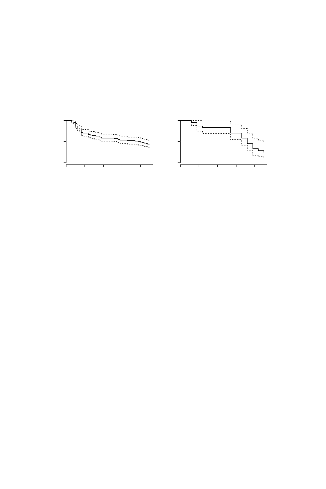
Argentina and Mexico: A Closer Look at Bank Bailouts

Figure 4.2: Non-parametric (Kaplan-Meier) estimates of bank survival in

Argentina and Mexico after the onset of the Tequila crisis. The solid line

corresponds to the mean survival rate; broken lines are 95% conﬁdence
intervals.

Argentina

Mexico

.51

Months from 12/1994

.51

Months from 12/1994

surviving banks in Argentina reﬂect a larger bank population as well as higher
observation frequency (months rather than quarters). Based on the observed
duration of banks, I estimate one-year survival rates to be 67.4% (with a 95%
conﬁdence band of 59.7–75.6) in Argentina, and 83.3% in Mexico (69.7–
99.7%). These estimates suggest that a government like Mexico’s would have
intervened or closed down 17% of banks a full year into a banking crisis,

whereas a government similar to Argentina’s would have forced the exit of

32%.

This ﬁnding comports well with the view that Bagehot governments

close insolvent banks promptly. However, one is still left to wonder whether
indicators of bank insolvency are good predictors of bank exit in Argentina,
as corresponds to a Bagehot government. The main indicator of ﬁnancial
insolvency is a bank’s capital-asset ratio. In principle, a bank’s CAR contains
su

ﬃcient information about its ability to withstand distress, and is therefore

the main indicator that regulators employ to decide whether a bank should
remain under shareholders’ control (Freixas and Rochet 1997, 275–279).
If the Argentine government acted as a stern Bagehot enforcer of market
outcomes, we would expect a bank’s CAR to be a negative predictor of its
hazard rate (alternatively, a positive predictor of bank survival or duration).
In contrast, we would not expect CAR to be a good predictor of bank duration
in Mexico if authorities in that country were indeed bailout-prone. I estimate
the association between a bank’s capital-asset ratio in December 1994 and
the length of its lifespan up to August 1998 in Argentina, or June 2000 in
the case of Mexico. Aside from CAR, I also include bank size (the value
of bank assets) as an additional regressor. I do so because some banks may

Curbing Bailouts

have been considered “too big to fail” (Stern and Feldman 2004); a Bagehot
government should in principle resist the urge to postpone exit of an insolvent
bank, regardless of size.

Table 4.3 summarizes the posterior distribution of e

ﬀect parameters in a

Bayesian exponential survival model.

Covariates CAR and bank size are

standardized, so their coe

ﬃcient estimates can be interpreted as the expected

change in the linear predictor of a bank’s hazard rate that would follow from
shifting values of covariates one standard deviation away from the mean.
Prima facie, it would seem that there is scant di

ﬀerence between Argentina

and Mexico in terms of their propensity to bail out larger banks. In both
cases, the coe

ﬃcient on bank size is centered about −1, and the posterior

distribution of this parameter is clearly bounded away from 0 (note that the
credible intervals do not straddle 0). A bank with CAR and bank size ﬁxed at

Argentina’s mean sample values would be expected to last about 38 months;

a bank one standard deviation larger than Argentina’s mean bank size would
survive about 105 months. In Mexico, comparable expected durations are

40 and 73 months. Not only are larger banks expected to last longer in both

countries, but capital-asset ratios are good predictors of bank survival in
both countries. Admittedly, better capitalized banks have lower hazards in

Argentina (–0.91) than in Mexico (–0.60), but even a Mexican bank with CAR

one standard deviation above the sample mean would be expected to survive
about 33 months longer than a bank with mean capitalization levels. Note,
however, that the posterior distribution of the CAR coe

ﬃcient in Mexico has

some probability mass on the positive orthant (the upper bound of the 95%
credible interval is 0.2). In practice, this means that, after controlling for bank
size, there exists a non-negligible probability that better capitalized banks

would survive less than ill-capitalized banks in Mexico. This is not the case

in Argentina: Larger banks may have been expected to survive longer periods,
but ill-capitalized banks faced a much larger chance of being forced out of
the system.

These inferences are premised on a rigid model of bank duration that fails

to take full advantage of information collected from balance-sheet data and
from known characteristics of the Argentine and Mexican banking systems. In

what follows, I account for three of these characteristics. First, the observed
values of CAR and bank size indicators vary not only across banks, but they

also change period-by-period and can vary drastically from one month or
quarter to the next. It would be desirable to incorporate this “time-varying”
information into an analysis of length of bank survival. Aside from CAR and

I stipulate normally-distributed priors centered at 0 and with low precision for all parameters

in the model (i.e.,

N(0, 0.001)—I stick to convention in expressing the spread of normal distribu-

tions as precisions rather than variances). This structure of priors has little e

ﬀect on posterior

distributions.

Argentina and Mexico: A Closer Look at Bank Bailouts

Table 4.3: Exponential models of bank survival in Argentina and Mexico.

Covariates are measured at the beginning of the observation window (Decem-
ber 1994). Estimates are median and 95% credible intervals of the posterior
distribution of e

ﬀect parameters.

Argentina

Mexico

Parameter

Median

95% CI

Median

95% CI

CAR

−0.907 −1.29 −0.56

−0.597 −1.56 0.20

Bank size

−1.007 −1.32 −0.71

−0.927 −1.80 −0.08

Intercept

−4.016 −4.30 −3.77

−2.964 −3.44 −2.50

bank size, I include loan concentration as a time-varying covariate. A bank
has more concentrated assets to the degree that it lends to similar ﬁrms and
households; concentrated banks are more fragile because they cannot hedge
against risks. My measure of loan concentration is a Herﬁndahl index of
the degree to which loans to a small number of economic sectors dominate
a bank’s balance sheet. In the case of Mexico, I also include the ratio of
non-performing to total loans (NPL ratio) as a further bank

/period predictor

of survival. Appendix A.2.1 reports all covariates used in the analysis.

Second, the process of bank exit was probably inﬂuenced by variables

that changed period-by-period but remained constant across banks. Changes
in the rate of economic growth at the national level (GDP change) or, more
germanely, the level of liquidity support from the central bank to the banking
system (CB credit) are variables that a

ﬀected the chances of survival of all

Argentine and all Mexican banks. In other words, bank

/quarter (bank/month)

observations in Mexico (Argentina) are nested within quarters (months) dur-
ing which system-level variables changed; it is therefore necessary to account
for this hierarchical structure in a more ﬂexible model speciﬁcation. Further-
more, the period-level covariates were markedly di

ﬀerent before than during

the banking crises; to compare the e

ﬀect of period-level covariates before

and during the crises, I extend the observation window backwards to 1991.
In the Mexican database I observe actual bank starting points, i.e., the date
at which banks were chartered as private enterprises. In Argentina, I have
extended the observation period back to March 1991, which coincides with
the end of the period of hyperinﬂation and, in essence, the start of a new era
in Argentina’s ﬁnancial system following the approval of the Convertibility
law and a new Central Bank charter later that year. Observing banks at an
early stage mitigates the problem of “left truncation” that threatens biased

Curbing Bailouts

inference in survival analysis.

Third, banks themselves vary markedly depending on their ownership

structure and the political prowess of bankers. This fact suggests that bank
survival may vary across bank categories in Argentina and Mexico. In Ar-
gentina, the setup of the banking system around 1994 suggests considering
three categories or bank types. Private banks with domestic majority partic-
ipation, traditionally organized around Argentina’s AdeBA, comprised the
ﬁrst group (80 banks). The second group was made up of large foreign banks

(34), which had increased their market share in the country even before the
Tequila crisis. The last group included cooperativas bancarias, or mutual

banks (42). As is common elsewhere, these tended to be smaller and had
less diversiﬁed assets. Because mutual thrift banks have no shareholders and
are much smaller than regular banks, it is possible that their closure imposed
lower political costs on regulators,

which would compromise their ability

to survive the crisis unscathed. By August 1998, banks in the ﬁrst group

went from 80 to 41, whereas only ﬁve mutual banks survived out of 42 at the

beginning of the observation window.

Legal impediments prevented foreign banks from entering the Mexican

banking system in full force before 1995; only two foreign banks operated in
Mexico at some point during the observation window, though naturally many
more entered as they took over failing domestic banks (see fn. 39). The other
banks in the system were owned by private investors, many of them from
the ranks of stockbroking companies that had ﬂourished during the boom
years of the Salinas administration and bid for banks during the privatization
process of 1991–1992. The larger banks, however, were controlled by active
members of the Consejo Mexicano de Hombres de Negocios (CMHN), an
informal lobbying organization that gathers some of the most inﬂuential
businessmen in Mexico (Teichman 1995). In Mexico, banker membership into
the CMHN may thus be associated with longer bank survival. In consequence,
I distinguish three bank types in this country: foreign (two banks), domestic
CMHN (5), and domestic non-CMHN (27).

To provide appropriate estimates of the association between ﬁnancial

status and bank duration, a model of bank survival must accommodate a
nested data structure in which indicators of interest vary at the bank

/period

level (CAR, bank size, and loan concentration), the period level (GDP change
and CB credit), and the bank level (bank type). In addition, the lifespans
of banks are highly correlated because the observation window includes a
period before the onset of the crisis during which only a handful of banks

Bank histories are left-truncated if their lifespans precede the beginning of the observation

window.

This view is expressed by Cole (1993, 301) for closures during the US S&L crisis.

Argentina and Mexico: A Closer Look at Bank Bailouts

exited the system, and a post-crisis period during which banks failed at
increasing rates. This correlation is an artifact of the way in which I set
up the observation window, and it should be controlled for in the model by
allowing the possibility of an increasing hazard rate. Thus, I consider the
baseline duration t of banks to follow a Weibull distribution; this assumption
allows me to accommodate hazard rates that increase throughout time.

To accommodate nested data levels, I model the scale parameter

μ of the

Weibull distribution as a function of bank

/period characteristics and period-

level covariates. Equations 4.1 and 4.2 display the basic structure of the
model:

i j

∼ Weibull(ν, μ

i j

)

(4.1)

i j

= exp(α

+ γZ

i j

+ βX

)

(4.2)

Because at the lowest level of aggregation data vary by bank

/period, the

dependent variable is the length of survival (in months or quarters) of bank i
in period j. If bank i has not exited the banking system in the last period of
observation (the 90

month in Argentina, the 35

quarter in Mexico), then

the survival distribution is a truncated Weibull.

I include a vector of random

ﬀects α

to allow for di

ﬀerent frailties or heterogeneity in underlying hazard

rates across bank categories (k

∈ {1, 2, 3} corresponding to foreign, private,

and mutual banks in Argentina and to foreign, private, and CMHN banks in
Mexico). Coe

ﬃcients γ and β are the eﬀect parameters for covariates that

vary at the bank

/period and period levels, respectively. To complete the model

setup, I stipulate proper but di

ﬀuse priors on model parameters; diﬀuse prior

distributions have negligible impact on posterior distributions.

I ﬁt the hierarchical Weibull model of Equations 4.1 and 4.2 to Argentine

and Mexican bank balance-sheet data.

Summaries of the posterior distri-

bution of parameters appear in Table 4.4; recall that negative coe

ﬃcients

imply lower hazard rates and, consequently, longer bank durations (except
for shape parameter

ν, where the opposite relation holds). There are sev-

eral noteworthy ﬁndings, which I discuss brieﬂy before reconsidering the

Because few exits appear at early periods but exits start bundling together at later dates,

I expect the shape parameter

ν of the Weibull distribution to be larger than 1. This would be

consistent with a survival process in which failures are uncommon at the beginning, but occur

with high probability toward the end of the observation window.

This arrangement permits the piecewise estimation of the hazard function. As can be

glimpsed from Figure 4.2, right censorship is more common in the Argentine bank population
(72 banks that were already established in March 1991 survive throughout the entire observation

window), but the rate of censorship is not identical across categories of banks.

The prior distributions are

α, β, γ ∼ N(0, τ = 0.001); ν ∼ Gamma(1, 0.001).

The Winbugs code appears in Appendix A.3.1. Inferences are based on 1,000 draws (thinned

every 10

value) of two chains started at dispersed initial values, after dropping the ﬁrst 1,000

draws. Convergence was monitored using the Gelman-Rubin R

statistic.

Curbing Bailouts

Table 4.4: Weibull models of bank survival in Argentina and Mexico, with

time-varying covariates, period-speciﬁc covariates, and random e

ﬀects for

bank type. Estimates are median and 95% credible intervals of the posterior
distribution of e

ﬀect parameters.

Argentina

Mexico

Parameter

Median

95% CI

Median

95% CI

Bank

/quarter time-varying covariates

CAR

−1.27

−1.34 −1.20

−0.02

−0.15 0.12

Bank size

−0.31

−0.33 −0.29

−0.78

−0.91 −0.62

Loan conc.

.05

.02 0.07

.14

.06 0.21

NPL ratio

−0.029 −0.11 0.05

Quarter time-varying covariates

GDP change

.74

.71 0.77

−0.49

−0.57 −0.41

CB loans

.71

.69 0.74

.14

.06 0.21

Bank type intercepts

Private bank

−8.41

−8.55 −8.28

−5.06

−5.43 −4.72

Mutual

−8.42

−8.54 −8.27

CMHN

−4.33

−4.67 −3.95

Foreign bank

−8.43

−8.56 −8.30

−5.47

−5.95 −5.04

Base hazard

.34

.30 2.37

.96

.85 2.08

Survival (

.83

.37 34.29

.96

.26 11.59

Survival (–)

.70

.36 27.12

.94

.37 11.55

10,389

702

Banks

156

Periods

90 months

35 quarters

nexus between ﬁnancial status and bank survival. First, despite employing
a non-informative prior on the shape of the baseline hazard rate I ﬁnd that
the risk of exit increases with bank duration (the posterior distribution of
ν lies entirely above 1 in both countries). This is not surprising given that
a majority of failed banks in both countries started their lifespans during
the ﬁrst observation period and exited the system within a relatively short
time halfway through the observation window after the banking crisis started.
Second, I observe noticeable di

ﬀerences in the survival of banks according to

their type in the case of Mexico, but not in Argentina. Consider Argentina

Argentina and Mexico: A Closer Look at Bank Bailouts

ﬁrst: After controlling for bank size, there is practically no di

ﬀerence in the

distribution of the coe

ﬃcients that correspond to the three diﬀerent bank types

(private, mutual, and foreign). In particular, despite the fact that mutual banks

failed at larger rates and their assets were often merged into private banks, it

would be di

ﬃcult to argue that there was a diﬀerential exit policy for banks

based on their ownership structure or idiosyncratic lobbying capacity. Any
variation in failure rates between private banks and mutual banks is accounted
for by di

ﬀerences in bank size and capitalization levels, especially the latter.

In other words, it is hard to believe that high rates of failure among mutual
banks were the result of an orchestrated e

ﬀort to beneﬁt private banks at the

expense of cooperativas bancarias.

In contrast, di

ﬀerent types of banks in Mexico show diﬀerent frailties.

These frailties defy expectations, as results suggest that banks owned by

members of the Consejo Mexicano de Hombres de Negocios enjoyed shorter
staying power than non-CMHN banks, after controlling for size and capi-
talization. The expected bank duration of a CMHN bank was 6.31 quarters

when holding all variables constant at sample means; non-CMHN banks
were expected to survive 9.13 quarters. Consider however that bank size and

CMHN membership are very highly correlated (the mean log size of CMHN
banks is 11.6, 8.9 for non-CMHN banks). In fact, we do not observe small
CMHN banks, which would be an oxymoron. Results are therefore consistent

with the view that CMHN banks survived longer than non-CMHN banks

because of sheer size, and not necessarily on account of the lobbying power
of CMHN bankers. An average-sized CMHN bank has expected duration
equal to 10.35 quarters, whereas an average-sized non-CMHN bank was
expected to live 8.20 quarters, all else constant. Aside from bank size, a larger
index of loan concentration is associated with slightly lower bank duration,
but the e

ﬀect is substantively negligible (in Mexico, for example, a drop in a

bank’s loan concentration index of one standard deviation below the sample
mean increases expected survival by less than three months).

I include short-term GDP change and central bank liquidity support as

covariates that a

ﬀect all banks within a period but vary across periods. My

decision to include GDP change follows from the expectation that shifts in na-
tional economic fortunes ought to a

ﬀect bank balance-sheet items, especially

if a severe economic downturn limits the ability of bank debtors to pay their
loans. Furthermore, changes in GDP may also a

ﬀect the political decision

to close insolvent banks, though the direction of this e

ﬀect is not entirely

clear. In fact, I ﬁnd that the association between period-to-period changes in

Admittedly, the capitalization levels of private banks may have been improved because of

preferential access to government-sponsored capitalization programs. I cannot disavow this
explanation with the data at hand. However, recall the various quandaries set up by the Argentine
government to prevent access by ex ante insolvent banks to capitalization funds.

Curbing Bailouts

GDP and bank survival is di

ﬀerent in Argentina and Mexico. In Argentina,

positive GDP change is associated with an increase in the mean hazard rate
across banks; the opposite association holds in Mexico. More interestingly,
an increase in CB credit is associated with an increase in the mean hazard
rate in both countries. Because the Argentine and Mexican models are based
on di

ﬀerent samples, the eﬀect on bank duration of changes in central bank

expenditures are not directly comparable. However, the positive association
between CB credit and hazard rates is consistent with the lender of last resort
role that central banks in both countries played during their banking crises—
indeed, we would expect central bank liquidity injections and bank closures
to be much more frequent during banking crises than during tranquil periods.

The main parameters of interest are the coe

ﬃcients for CAR and, in the

case of Mexico, NPL ratio. These coe

ﬃcients reveal the extent to which

the bank exit process in these countries reinforced or counteracted market
outcomes. In Argentina, we see that a bank’s capital-asset ratio is a substan-
tively important predictor of expected survival, even after controlling for an
array of bank- and period-level covariates. In short, better capitalized banks
had lower hazard rates. In Table 4.4, the rows labeled “Survival” display the
distribution of median survival times for banks with low capitalization levels

(25

percentile of the sample distribution of CAR) and high capitalization

levels (75

percentile). Median survival times correspond to the number of

periods that one would need to wait to see the exit of 50% of banks in a
population. The posterior distribution of these survival times suggests with
very high probability (0.95) that the median Argentine bank in a set of well-
capitalized institutions would survive between 33.4 and 34.3 months, holding
all covariates constant at mean levels. In contrast, the median ill-capitalized

Argentine bank would live between 26.4 and 27.1 months. Compare these

predictions against those that obtain in the Mexican sample: there is in fact
no di

ﬀerence in the expected length of median survival of well- versus ill-

capitalized banks. Simply put, capitalization levels are not good predictors of
bank exit in Mexico. Furthermore, non-performing loan ratios are also useless
as predictors of bank survival in that country. In short, Mexican politicians
seem to have considered bank size as the sole criterion to determine bank
exit.

4.3 Concluding Remarks

The analysis of bank survival in Section 4.2.2 resonates with the depiction of
Argentina and Mexico as, respectively, Bagehot and Bailout governments. In

This result is not an artifact of collinearity between NPL and capital-asset ratios. Though

the correlation between these variables is negative, as one would expect, and relatively strong
(

ρ = −0.32), similar results obtain when excluding NPL ratio from the model.

Argentina and Mexico: A Closer Look at Bank Bailouts

Argentina, the Menem administration was relatively quick in enabling regu-

latory agencies to combat bank liquidity and insolvency problems. Though
only three banks had been suspended two months into the banking crisis

(Basel, Finansur, and Trader), the Easter legislative package granted ﬁnancial

authorities the power to close several other ﬁnancial institutions right away.

With the power to allocate assets, intervene banks, and subsidize mergers of

bad banks into good banks, Argentine regulators forced the exit of a large
number of insolvent ﬁnancial institutions expeditiously. By election day on
May 14, the bank run that had started with the December devaluation of the
Mexican peso had abated, and bankers and regulators were starting to get a
handle on remaining insolvency issues. Though my analysis suggests that
the Argentine government was not immune to “too big to fail” considera-
tions, capitalization levels are unarguably important predictors of bank exit,
as corresponds to a Bagehot enforcer. In contrast, capitalization levels are
irrelevant in understanding bank exit in Mexico. The Mexican authorities did
not readily implement a comprehensive program to cope with the banking
crisis, despite the fact that banking agencies (Fobaproa and CNBV) were
not equipped to deal with the grievous insolvency problems that a

ﬀected do-

mestic banks. Instead, the Zedillo administration pushed through a pastiche
of crisis-management programs that were not necessarily out of line with
restructuring policies elsewhere, but did not seem to follow a coherent plan
based on sober assessments of insolvency either.

Some preliminary lessons can be drawn from these two experiences of

bank crisis response. First, banking crises are costly a

ﬀairs, even when gov-

ernments limit the size of ﬁnancial losses transferred to taxpayers. In order
to deal with ﬁnancial insolvency, the Argentine taxpayer subsidized mergers
of good and bad banks and the monetary authority was granted the ability to
perform last-resort lending functions. Some would characterize these subsi-
dized operations as “bank bailouts” because they amounted, in essence, to the
continuation of bad banks under di

ﬀerent names and/or to the continuation

of illiquid banks. This indiscriminate use of the term “bailout” is essentially
useless, as it throws in the same bag very di

ﬀerent crisis-management styles.

Instead, my interpretation of bailouts corresponds to an essentially continuous
construct that measures the amount of ﬁnancial losses that are passed on to
the taxpayer. In this sense, policies to contain and redress banking crises run
the gamut from taxpayer absorption of all ﬁnancial losses derived from bank
insolvency to more limited taxpayer help to restructure a distressed bank-
ing sector. Crisis-management policies reveal ample information about the
bailout propensities of di

ﬀerent governments. Analyzing bailout propensities

is the ﬁrst step towards verifying the existence of political regime e

ﬀects on

banking policies.

Second, the institutional setup of banking agencies may have an impact

Curbing Bailouts

on the way in which banking crises are managed, but though it is common
to argue that banking agencies matter it is less obvious which features are
consequential. Furthermore, the structure of bank supervision and regulation
seems to be endogenous to political decisions to cope with banking crises. It
is clear that the governments of Argentina and Mexico scrambled to grant
old and new banking agencies the ability to deal with insolvent banks. In
this regard, it is noteworthy that Argentine policy-makers were able to tweak
the currency board arrangement so that the BCRA could carry out LOLR
functions. When it comes to reforming banking agencies, it is not uncommon
to see governments patching the ship at sea. The Argentine authorities took
advantage of the crisis to strengthen their bank supervisory institutions and
to develop bank restructuring expertise while keeping down costs passed on
to the taxpayer. Instead, Mexican o

ﬃcials designed a series of policies that

varied in their ability to elicit optimal banker behavior. On one extreme, the
temporary capitalization programs limited moral hazard incentives. On the
other extreme, the set of policies coordinated through Fobaproa to purchase
bad assets in exchange for fresh capital ended up providing the worst possible
incentives to bankers. In contrast with the high-powered incentives that were
built into Procapte to keep ﬁscal cost low, Fobaproa seemed purposefully
planned to transfer most bank losses to the taxpayer.

Finally, my choice of Argentina and Mexico as exploratory cases was

not due to my a priori perception of their policy responses, but to the fact
that while Argentina could be depicted as a consolidated, albeit imperfect,
democratic regime by 1994, Mexico was still in the midst of transition towards
full electoral contestability by the time the crisis hit. My main theoretical
claim is that democracies are better able to withstand pressures to transfer
losses to disorganized taxpayers simply because the latter can make their
voice heard during elections. In this regard, one could imagine that facing
elections in the near future would have the opposite e

ﬀect to the one posited

here, i.e., that elected politicians fear the wrath of their constituents and are
therefore likely to extend the lives of insolvent banks if elections are close in
the horizon. In Argentina, before the Easter presidential decrees that ended
the deposit run were implemented, there was indeed some speculation that the
government could ignore the problem until after the elections. Politicians in
democratic regimes may well choose to engage in regulatory forbearance in
expectation of an electoral contest and therefore increase taxpayer costs, but
in order to validate my theoretical claim the relevant counterfactual scenario
is not that of a democratic regime without elections in the immediate future,
but that of an election-less authoritarian regime or, more likely, one with
limited electoral accountability.

An obvious candidate mechanism to explain why democracies may be

less prone to bailouts is the existence of multiple veto points. The idea that

Argentina and Mexico: A Closer Look at Bank Bailouts

democratic regimes with very di

ﬀerent institutional features can be usefully

compared through analysis of the number of veto players in assemblies
and the executive power has been developed by Tsebelis (2002). From a
theoretical point of view, it is not entirely clear whether we should expect
veto points to increase or decrease the probability of bailouts. While it is
possible that veto players with di

ﬀerent policy positions could slow down

attempts to respond to a banking crisis, this conﬁguration could presumably
also lead to checks-and-balances that might improve policy-making (Haggard
and MacIntyre 1998). I ﬁnd no reason to believe that a veto points argument
could help understand Argentina’s response. Congressional participation in
revamping ﬁnancial laws was minimal at best and, as was common during his
tenure, President Menem passed many relevant reforms by decree. In Mexico,
President Zedillo’s administration avoided immediate major reforms and
coordinated the bailout e

ﬀort through the Ministry of Finance and Fobaproa.

But in line with a veto point logic, a major e

ﬀort to review bailout policies

and revamp ﬁnancial losses was put in motion once midterm elections in 1997
returned a more fractious lower Chamber. At that point, though, ﬁnancial
losses derived from bank insolvency had been apportioned and Mexican
taxpayers had already acquired hefty obligations.

Suggestive as it may be, the paired Argentina-Mexico comparison is ulti-

mately limited for two main reasons: First, as in many qualitative analyses,
it is di

ﬃcult to guarantee that these two cases are representative of the ways

in which democracies and autocracies react to banking crises. One cannot
rule out the possibility that the policy reactions of Argentina and Mexico
are outliers within the populations of, respectively, democratic and semi-
authoritarian regimes. Second, even if Argentina and Mexico in 1991 through

1999 were typical cases within the populations of democracies and authori-

tarian regimes, we are still unable to conﬁdently attribute variations in their
observed responses to di

ﬀerences in their political regimes. Political regime

is one of the attributes that varies across these cases, but it is certainly not
the only meaningful di

ﬀerence between these two countries. Consequently,

throughout the rest of the book I base inferences about regime e

ﬀects on

inspection of a larger set of cases.

Variation in Government Bailout Propensities

Chapter 4 dissected the policy response to systemic banking crises during the
mid-1990s of two governments, a democratic regime that carried out policies
close to the Bagehot ideal-type and a semi-authoritarian regime that pursued
policies closer to Bailout. The analysis in that chapter is consistent with
the main proposition of this book, namely, that politicians in democracies
react di

ﬀerently than politicians in autocracies whenever they confront wide

insolvency in the banking sector. However, Argentina and Mexico were
di

ﬀerent not only in their political regimes, but also along dimensions that

may help account for their policy choices, from the institutional setup of
the monetary authority to the structure of their banking systems. Some
of these factors—like supervisory stringency, or extension of crony links
among entrepreneurs, bankers, and government—are theorized to follow from
variations in political regime, but some others—like international openness or
institutional constraints on the monetary authority—are not. Unfortunately,
one cannot control for potential confounding variables in a paired comparison.

To make progress in estimating the e

ﬀects of political regimes on banking

policies, I follow a di

ﬀerent strategy over the next chapters. Basically, I

consider variation across governments to assess the degree to which polit-
ical regimes matter in understanding policy responses to widespread bank
insolvency. Based on theory presented in Chapter 3, the political regime
under which governments operate should have an impact on the probability
of observing a bank bailout. In line with Proposition 1, I expect democra-
cies to be more successful in limiting burden-sharing with taxpayers upon
su

ﬀering a banking crisis. Aside from validating this hypothesis, the analysis

in this chapter and the next sheds light on other seldom-explored aspects of
management of banking crises, like the relative political expediency of alter-
native policies and the potentially multi-dimensional character of government
response. To fully present the evidence that substantiates Proposition 1, I

Variation in Government Bailout Propensities

break down the analysis into two chapters. In Section 5.1 of this chapter I ﬁrst
describe the data on which the analysis is based, a small sample of forty-six
documented instances of policy response to banking crises. In Section 5.2
I detail the modeling assumptions that allow me to reach inferences about
bailout proclivities based on the peculiar characteristics of observed data. In
particular, I rely on item-response theory models to build and analyze an indi-
cator of the bailout propensity of di

ﬀerent governments. Section 5.3 closes

with a preliminary analysis of the e

ﬀect of political regime on the decision of

governments to pursue Bagehot or Bailout, and Section 5.4 considers whether
recent instances of bailouts in democratic regimes provide enough evidence
to cast doubt on the existence of a democratic advantage. I build a case for a
causal interpretation of the impact of political regimes on bank bailouts in
Chapter 6. I conclude there that democratic regimes are indeed less likely to
carry out onerous bailouts.

5.1 Crisis-Management Policies

I argued in Chapter 1 that the concept of “bank bailout” is only useful if we
consider it as a theoretical continuum between the ideal-types of Bagehot and
Bailout, where outcomes closer to the latter extreme correspond to higher
burden-sharing with taxpayers. Every government redistributes losses derived
from bank insolvency to some extent; consequently, even the thriftiest gov-
ernment ends up burdening taxpayers with at least some portion of ﬁnancial
losses produced by the behavior of economic actors. To validate Proposi-
tion 1, I assess the bailout propensities of di

ﬀerent governments—i.e., the

degree to which these governments sheltered banks from the consequences of
insolvency. Recall that Proposition 1 states that democracies are more likely
to adopt harsher closure rules to deal with distressed banks.

The empirical analysis is based on a sample of government responses to

forty-six separate banking crises observed from 1976 to 2003. Most of these

were compiled, coded, and disseminated by Honohan and Klingebiel (2000);

I have complemented their database with information from Del Villar, Backal
and Trevi˜no (1997) and from secondary sources through Lexis-Nexis (see

Appendix A.2.3). These forty-six events are a subset of a larger collection

of episodes recognized by policy experts as systemic banking crises (see
Chapter 7). Though the subset of N

= 46 is relatively small and presumably

favors banking crises that were relatively well publicized, no obvious selection
bias is evident in the sample. In other words, democracies are not over-
represented over autocracies, corrupt over non-corrupt regimes, or open over
closed economies; in preliminary tests, not reported here, none of these
factors were signiﬁcant predictors of the inclusion of a banking crisis in the

Curbing Bailouts

sample (see Rosas 2006). The only partial exception is that poorer economies
tend to be slightly under-represented, in the sense that real per capita GDP is a
statistically signiﬁcant, albeit substantively unimportant, predictor of whether
a systemic banking crisis will appear in the sample. Thus, these 46 banking
crises are to a large extent representative of the wider universe of events. This
need not mean that policy responses themselves are representative, nor do
I make the claim that the distribution of treatment (democracy) and control
conditions across these observations is random. I will return in Chapter 6 to
the problem of making causal inferences based on observational data, where
the mechanism assigning treatment (democracy) and control (non-democracy)
is not known.

Honohan and Klingebiel provide details about governmental responses

to banking crises. Among other indicators, they code whether any of seven
policies commonly used to address bank solvency and liquidity problems

were implemented during a systemic banking crisis; they build a dichotomous

score for each of these seven policies within each banking crisis in the sample.

Table 5.1 reproduces their coding scheme. As can be gleaned from this table,

the seven binary indicators can be directly traced to the ﬁve policy issue-
areas—exit policy, liquidity support, asset resolution, liability resolution, and
bank capitalization—detailed in the Bagehot-Bailout classiﬁcation scheme of

Table 2.3. For example, bank liquidity is an indicator of government response

regarding protection of bank depositors that is coded “1” for governments
that extended emergency liquidity support during at least twelve months,

with overall support exceeding the total amount of banking capital (Honohan

and Klingebiel 2000). Table 5.1 shows how the other six indicators (for-
bearance, public asset management, debt relief, explicit guarantees, deposit
freeze, and recapitalization) relate to policy issue-areas in Table 2.3. The
last two columns of Table 5.1 display counts of the number of governments
that enacted each of the seven policies and the number of missing values in
each category. By far, the most popular interventions are provision of liquid-
ity through heavy last resort lending (23 cases) and regulatory forbearance

(28), whereas ﬂagrant cases of debt relief for corporate borrowers or bank

recapitalization with public funds are less common.

5.2 An Item-Response Theory Model of Bailout Propensity

We can exploit variation in the frequency with which these policies were

implemented to elicit information about the underlying bailout propensities
of di

ﬀerent governments; in fact, better inferences about bailout propensities

follow from consideration of all seven indicators as a set, rather than from ex-
amination of a handful, provided that these data are combined in a principled

able

5.1:

crisis-management

polic

indicators.

The

last

column

displays

the

number

ernments

(out

46)

that

implemented

the

corresponding

polic

response

banking

crisis

(missing

alues

parentheses).

Indicator

(Proxy

for

...)

Coded

(MV)

gulatory

forbear

ance

(Exit

polic

ernment

relax

fails

enforce

gulation

for

least

one

year

Bank

competition

restricted.

ernment

fails

shut

distressed

banks

after

three

months.

ernment

allo

insolv

ent

banks

continue

under

original

management.

(2)

Bank

liquidity

(Liquidity

support)

ernment

pro

vides

liquidity

support

lar

ger

than

total

banking

system

capital

insolv

ent

banks

for

least

one

year

(2)

Public

asset

mana

ement

(Asset

resolution)

ernment

transfers

non-performing

bank

loans

centralized

public

asset

management

corporation.

(1)

Debt

relief

(Asset

resolution)

ernment

sponsors

debt

relief

for

corporate

borro

wers,

through

exchange

rate

guarantees

direct

rescue.

(5)

Explicit

guar

antees

(Liability

resolution)

ernment

issues

explicit

deposit

guarantee.

State-o

wned

institutions

hold

75%

total

banking

deposits.

(2)

Deposit

eeze

(Liability

resolution)

ernment

freezes

deposits

interv

ened

banks

for

least

one

year

(2)

Recapitalization

(Bank

capitalization)

ernment

recapitalizes

banks

through

one-shot

support

scheme.

ernment

recapitalizes

banks

through

repeated

rounds.

(1)

100

Curbing Bailouts

manner.

I model government responses to banking crises using tools from item

response theory (IRT). These models are extremely ﬂexible tools to ana-
lyze limited dependent variables, particularly the kind of data—dichotomous
variables—described in Table 5.1.

The basic setup of IRT models makes

them ideal tools to analyze policy problems in which a set of dichotomous
variables can be interpreted as manifest indicators of some latent policy con-
struct. In this case, I construe the seven policies laid out in Table 5.1 as
manifest indicators of a government’s latent bailout propensity. We can then
use IRT models to make inferences about unobserved tendencies that push
politicians to enact alternative policies. In this section, I relate informally
the various assumptions underlying IRT models of bank bailouts, abstracting
from more technical issues about identiﬁcation and estimation. I ﬁt several
models to the data described in Table 5.1; these models vary mostly in the
amount of information they incorporate about government characteristics
and the assumptions they make about the seven crisis-management policies,
but they all start from the premise that government i’s unobservable bailout
propensity

drives the distribution of observed policy responses y

, j

= {0, 1}

(i is the government index, j is the policy index). The unit of analysis is thus

a government’s response to a banking crisis, with seven dichotomous policy
indicators per observation. Many countries su

ﬀered multiple banking crises

during the period under inspection, but only ﬁve of these—Argentina, Indone-
sia, Malaysia, Mexico, and Turkey—provide more than one observation to
the dataset.

To understand how an IRT model helps us extract information from these

data, recall from Table 5.1 that the number of governments that implement
each of the seven crisis-management policies varies a great deal, from a
minimum of ten countries pursuing debt relief to a maximum of 28 countries
adopting regulatory forbearance. These di

ﬀerences speak to the relative ease

with which governments can pursue di

ﬀerent policies; in other words, it is

reasonable to assume that the sample frequency of these policies reveals the
degree to which these policies are politically expedient. For example, regu-
latory forbearance often starts with low-level bureaucratic decisions that do
not immediately invite oversight from, or require the benediction of, elected
government o

ﬃcials. Even when regulatory forbearance is the result of direct

Previous research has used some of these dichotomous variables as indicators of selected

aspects of Bagehot-Bailout (for example, Keefer 2002 uses forbearance and Nava-Campos 2002
combines explicit guarantees, bank liquidity and forbearance in an additive index).

See Rasch (1980) for an introduction to IRT models and Johnson and Albert (1999, ch. 6)

for IRT models in a Bayesian framework.

I count each banking crisis as an independent observation, i.e., observations are not clustered

within governments. This is not unreasonable given that banking crises do not occur within the

same government, even if they occur within the same country.

Variation in Government Bailout Propensities

101

intervention from “up high,” this policy is relatively easy to implement, as it
requires a passive “response.” Instead, policies such as debt relief or bank
recapitalization often require legislative intervention or concerted action by
a variety of agencies, and are therefore relatively di

ﬃcult to pursue, even

by governments with high bailout propensity. Moreover, these two policies
create immediately recognizable outlays that must be met with taxpayers’
money. Relatedly, provision of bank liquidity is generally the province of a
nation’s central bank, which may or may not be autonomous from politicians.
In any case, crisis-management policies are subject to political constraints
of varying importance. In an IRT model, the overall political expediency of
enacting each of the seven policies would be captured by a set of parameters
α

, which are appropriately labeled di

ﬃculty parameters.

5.2.1 Inferences Based on Frequency of Policy Implementation

With these deﬁnitions in place, consider now the model of bailout propensities

across governments conveyed by Equations 5.1 and 5.2:

i j

∼ Bernoulli(π

i j

)

(5.1)

i j

= Φ(θ

− α

)

(5.2)

In Equation 5.1, each dichotomous policy item y

, j

is modeled as a random

draw from a Bernoulli distribution with parameter

, j

∈ [0, 1]—i.e., we as-

sume that y

, j

will take on a value of 1 with probability

, j

. Equation 5.2 then

considers parameter

, j

to be a function of item di

ﬃculty α

and government

bailout propensity

: The probability of observing policy j in response to

a banking crisis increases with the political expediency of the policy (lower
values of

α) and with the bailout propensity of the government (higher values

θ). These are the two core assumptions of the IRT model.

The main goal

in this case is to estimate bailout propensities

for all 46 governments based

on observable policy choices y

, j

; however, the model requires estimation

of di

ﬃculty parameters α

as well. Incidentally, notice that item parameters

vary across policies but are constant across governments, whereas bailout
propensities appropriately vary across governments.

In this baseline setup, the IRT model requires estimation of 46 bailout

propensities and seven item di

ﬃculty parameters, based on information from

× 7 observed policy values, so there is in principle suﬃcient information

to uniquely estimate model parameters. Note however that parameters

θ and

α are invariant to changes in scale and rotation, and therefore the model as

This model assumes a probit link for the Bernoulli parameter

i j

(

Φ is the standard normal

cumulative distribution function). Bear in mind that

α and π are parameters of a statistical model;

these are not the same as the democracy weight and risk proﬁle in Chapter 3.

102

Curbing Bailouts

expressed in Equations 5.1 and 5.2 is not identiﬁed. In other words,

θ and

α could be multiplied by any constant value and model ﬁt would remain
unchanged. One advantage of the Bayesian estimation of IRT models is
the possibility of using prior probabilities on parameters

θ and α to identify

the model. In the baseline setup, I ﬁx the scale of bailout propensities
by stipulating a standard normal prior distribution on parameters

θ as is

customarily done in this kind of model (Johnson and Albert 1999). This
prior solves scale invariance by constraining the bailout propensity of the
average government to be 0 and all other values of

θ to fall within a narrow

range around 0 (i.e., we assume a priori that 95% of all bailout propensities

will fall within –2 and 2). By the same token, I stipulate that the prior

distribution of di

ﬃculty parameters α is normal with mean 0 and standard

deviation

√

This prior distribution ensures that policies with average

degrees of di

ﬃculty or political expediency will get a score of α ≈ 0, and it

also allows the posterior distribution of di

ﬃculty parameters of all policies

to be lower (or higher) than the lowest (largest) bailout propensity. The
latter condition implies admitting a priori that some policies might not be
extremely informative about bailout propensities. In other words, we could in
principle see a policy that is so politically expedient (

lower than the lowest

) that all governments stand a better than even chance of implementing it,

regardless of how bailout-prone they are. Note that though prior probabilities
on parameters

θ and α are informative, this information is added to the model

with the sole purpose of achieving identiﬁcation. Inferences about

θ are still

largely data-driven and not overtly dependent on selection of priors.

Estimates of di

ﬃculty parameters for the model based on Equations 5.1

and 5.2 appear in the ﬁrst column of Table 5.2 (the point estimate corresponds
to the median of the posterior distribution, the standard deviation of the poste-
rior distribution appears in parentheses). The conclusions that follow from
the baseline model about the comparative expediency of alternative crisis-
management policies are not surprising given knowledge of the frequency

with which they have been adopted, but they conﬁrm the basic adequacy of

the IRT model.

Recall that a policy with parameter

α ≈ 0 corresponds to a

policy with “average” di

ﬃculty in the sample. Consistent with their relative

frequency in the sample, policies with di

ﬃculty parameters well above 0—

Note that this model is still invariant under rotation, so all

θ and α parameters could be

multiplied by

−1 and ﬁt would remain identical. To identify the model, I placed a non-positive

constraint on the bailout propensity of Argentina 1995, along with a non-negative constraint on
Mexico 1994 (cf. Jackman 2000). This implies that Mexico 1994 cannot have a lower bailout
propensity than Argentina 1995, an assumption entirely supported by the analysis in Chapter 4.

Estimates in Table 5.2 are based on 1,000 draws thinned every 10

draw after apparent

convergence from the joint posterior pdf of parameters. I ran two chains for 1,000 iterations
as burn-in for every model and assessed convergence based on the Gelman-Rubin ˆ

R statistic.

Convergence in these models was swift and clean.

Table 5.2: Bayesian estimation of Bagehot-Bailout policy (

α, β) and case (δ)

parameters. Point estimates are the median of parameter posterior densities

(standard deviation of parameter posterior densities in parentheses).

Parameters

Model 1

Model 2

Model 3

Model 4

.302

.377

.370

.339

.257)

.317)

.319)

.322)

.797

.904

.889

.908

.271)

.325)

.323)

.342)

.203

.292

.255

.245

.251)

.311)

.286)

.302)

F B

−0.452

−0.443

−0.450

−0.452

.258)

.233)

.256)

.251)

−0.822

−0.062

−0.052

−0.059

.240)

.202)

.190)

.802

.714

.679

.689

.268)

.225)

.213)

.221)

.245

.235

.232

.229

.254)

.196)

.201)

.199)

.389

.342

.399

.468)

.418)

.453)

.306

.182

.278

.412)

.401)

.412)

.400

.192

.288

.445)

.442)

.482)

F B

.673

.589

.724

.365)

.335)

.412)

.221

.079

.244

.218)

.258)

.201)

.275

.186

.313

.243)

.302)

.242)

.254

.238

.310

.222)

.281)

.217)

δ(democracy)

−0.324

−0.198

.192)

.189)

DIC

395

.74

374

.28

371

.73

374

.84

.16

.80

.67

.37

Model 3 based on dichotomous, 4 on continuous, democracy index

= liquidity, D = debt relief, AM = asset management agency, R = recapitalization,

= explicit guarantees, F = deposit freeze, FB = forbearance

104

Curbing Bailouts

Figure 5.1: Estimates of di

ﬃculty and bailout propensity parameters in a

common space. Point estimates are medians of the marginal posterior density
of each parameter (FB

= forbearance, L = liquidity, G = explicit guarantees,

= debt relief ).

Arg ’95

Fin ’91

Mex ’94

F B

debt relief and bank recapitalization—are relatively hard to implement; in
contrast regulatory forbearance is comparatively easy. In other words, many
governments ﬁnd it expedient to engage in regulatory forbearance, even those
that do not have particularly high bailout proclivities. Instead, a policy like
bank recapitalization, which requires investment of hefty public resources to
keep insolvent banks in operation will be approached with trepidation even
by the most bailout-prone government. Thus, the ease with which di

ﬀerent

governments enact these policies does not necessarily refer to the number of
bureaucratic levers that need to be pulled, or the complexity of the process
that needs to be set in motion, though admittedly this kind of mechanisms
are probably at the heart of variation in policy di

ﬃculty. Instead, “relative

ease” should be interpreted as the extent to which governments with di

ﬀerent

bailout propensities would choose these policies. Regulatory forbearance
is very common in the sample, which makes this an “easy” policy item;
therefore, observing that a government engages in forbearance only tells
us that the government’s bailout propensity is probably not extremely low.

This also suggests why sole reliance on regulatory forbearance to infer the

bailout propensity of governments would lead to incorrect inferences: Since
regulatory forbearance is comparatively easy, many governments that are
not particularly prone to Bailout still implement this policy; by inspecting
just one indicator, we would be characterizing even these governments as
reckless spendthrifts that place large ﬁnancial burdens on taxpayers. By a
similar argument, inspection of a subset of these seven indicators cannot be
preferable to a principled analysis of the full set.

To illustrate how the IRT model helps us make sense of government

Incidentally, the posterior distribution of

α tends to be wider for policies with more missing

values, as one would expect. The data-augmentation step proposed by Albert and Chib (1993) to
estimate the IRT model in a Bayesian framework allows multiple imputation of missing values
within the updating algorithm itself. This imputation process is valid under the assumption of
ignorable missingness (see Little and Rubin 1987; Rubin 1976).

Variation in Government Bailout Propensities

105

proclivities, Figure 5.1 displays the spatial position of policy di

ﬃculty pa-

rameters and bailout propensities for selected governments. The graph shows
point estimates (medians of the posterior distribution) of di

ﬃculty parameters

for four policies: regulatory forbearance (

F B

), liquidity (

), explicit guar-

antees (

), and debt relief (

). Alongside these parameters, I plot point

estimates of the bailout propensities of three governments that faced banking
crises during the 1990s: Argentina 1995, Finland 1991, and Mexico 1994.
Mexico appears as a government with extreme bailout propensity, consistent

with multiple accounts of this crisis and with the thrust of the analysis in

previous chapters. Also consistent with those views, Argentina comes very
close to fulﬁlling the spirit of Bagehot’s prescription by obtaining a very
low

θ score. Based on Figure 5.1, we would expect a government with the

bailout propensity of Mexico in 1994 to enact all four of the policies plotted
in the graph; a government with the characteristics of Argentina in 1995

would not be very likely to implement any of these policies. In contrast,

governments with average bailout propensity (

θ ≈ 0, like Finland in 1991)

would be expected to implement liquidity and forbearance, but not debt relief

or explicit guarantees.

5.2.2 Inferences Based on Varying Policy Discrimination

The model based on Equations 5.1 and 5.2 is still unnecessarily restrictive

in some important ways. One implicit assumption of this model is that all
crisis-management policies are equally good at distinguishing among govern-
ments with di

ﬀerent bailout propensities. In this context, the discrimination

potential of a given policy can be understood as its ability to separate Bailout-
prone from Bagehot-prone governments. A policy with high discrimination
potential would o

ﬀer a crisp cutpoint in the policy space represented in Fig-

ure 5.1; governments with bailout propensities to the right of this cutpoint

would implement the policy with very high probability. In contrast, policies
with low discrimination potential do not allow us to distinguish the policy

ﬀects of diﬀerent bailout propensities with great precision. Another way

of interpreting the discrimination potential of a policy is as follows: The
probability that a government will adopt policy j that has average di

ﬃculty

(

≈ 0) is about even, regardless of the government’s bailout propensity, if

its discrimination potential is nil (

≈ 0). As discrimination potential be-

comes larger, the policy provides more information about underlying bailout

These statements should be properly interpreted in a probabilistic fashion. Indeed, we can

use draws from the joint posterior distribution of all parameters to provide educated guesses about
the probability of observing di

ﬀerent events of interest. For example, based on the baseline model,

the probability that a government with Mexico’s bailout propensity will implement all seven
policies would be about 0.63. The probability that a government with Finland’s characteristics

would implement liquidity is estimated at around 0.33.

106

Curbing Bailouts

propensity. The assumption of equal discrimination is not necessary for
identiﬁcation purposes, and as I show below it receives no support from data.
Consequently, I extend the baseline predictor in Equation 5.2 so that it now
depends on a second policy-speciﬁc discrimination parameter

, as shown in

Equation 5.3:

, j

= Φ(β

− α

)

(5.3)

I expect all item discrimination parameters to be non-negative, which sug-

gests that governments closer to the Bailout ideal-type are in principle more
likely to implement the policies captured by the seven dichotomous indicators.
Consistent with this expectation, I stipulate a normal prior distribution on
β centered at 1 and with standard deviation 2. The prior mean of 1 implies
a moderate level of discrimination for items that have average di

ﬃculty. A

prior standard deviation of 2 assigns high probability to positive values of
β

while still placing enough probability mass on negative numbers to allow

the possibility that some policies might actually have negative discrimination
after updating. For example, ﬁnding that regulatory forbearance had negative
discrimination would imply that Bailout-prone governments are less likely to
adopt this type of policy, which would of course be contrary to theoretical
expectations.

Estimates based on Equation 5.3 are summarized in the second column

of Table 5.2 (Model 2). To understand how policy parameters

α and β

translate into predictions about policy implementation consider Panel a in
Figure 5.2, which plots item response curves of explicit guarantees and bank
liquidity based on estimates of Model 2. The graph suggests that explicit
guarantees and bank liquidity have very di

ﬀerent potential to discriminate

among governments with varying bailout propensities, even though both
of these policies have average di

ﬃculty parameters. Figure 5.2 also plots

estimates of the bailout propensities of Argentina and Mexico, along with
predicted probabilities of enacting these policies. Based on estimates of the
di

ﬃculty and discrimination parameters of explicit guarantees from Model

2 (i.e., ˆ

and ˆ

), one would expect a government with bailout propensity

similar to that of Mexico in 1994 (

Mex ’94

≈ 1.31) to implement this policy

with probability 0.7. The probability that a country like Argentina (

Arg ’95

≈

−0.93) would enact this policy is essentially 0. Contrast these results with
those that obtain from considering bank liquidity: Despite obvious di

ﬀerences

in the bailout propensities of Argentina and Mexico, the probability that these
governments would implement generous bank liquidity policies is not that
di

ﬀerent (0.13 and 0.25, respectively). The discrimination potential of bank

Incidentally, this prior distribution solves the problem of rotational invariance: Governments

with high values of

θ are now unarguably governments with high bailout propensity.

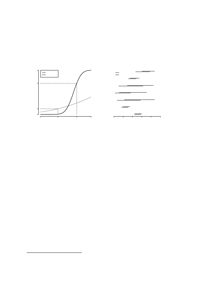
Variation in Government Bailout Propensities

107

Figure 5.2: Item response curves for explicit guarantees and bank liquidity
and predicted probabilities of implementation for Argentina and Mexico, and
probabilities of enacting crisis-management policies conditional on political
regime (bars represent 50% Bayesian credible intervals)

Bailout propensity

Probability of implementing policy

0.13

0.7

−3

Liquidity
Guarantees

Mex 94 = 1.305

Arg 95 =

−0.925

Probability of implementation

0.0

0.2

0.4

0.6

0.8

1.0

Liquidity

Debt relief

Asset mngt.

Recap.

Guarantees

Dep. freeze

Forbearance

Democracy
Non

−democracy

liquidity is very low, as one can see from the value ˆ

= 0.221 in the second

column of Table 5.2.

The extended model reveals that the discrimination parameters for asset

management corporation, recapitalization, explicit guarantees, and regula-
tory forbearance are bounded away from 0.

These policies, particularly the

ﬁrst one, are very sensitive to di

ﬀerences in the bailout propensity of govern-

ments. Three other policy items—liquidity provision, debt relief, and deposit
freeze—fail to display much discriminating power, as their posterior distribu-
tions are very close to 0. These three policies are all aimed at ameliorating
bank cash-ﬂow problems by either lending at a discount (liquidity provision),
preventing further drain on banks’ liabilities caused by indiscriminate deposi-
tor runs (deposit freeze), or supporting bank debtors so that they can continue
to make payments on outstanding loans (debt relief ). In other words, rather
than aiming to restore solvency in a distressed banking system, these policies
could be best understood as measures to manage liquidity problems during a
banking crisis. In Chapter 6, I consider the possibility that a second liquid-
ity dimension underlies government action, and explore whether political
regimes also determine bailout propensities along this second dimension.

Minor changes in the estimates of parameters

α obtain in Model 2—particularly in the case

of bank liquidity—upon estimation of parameters

β.

108

Curbing Bailouts

5.3 Bagehot, Bailout, and Political Regimes

I devote extensive attention to the estimation of item-speciﬁc parameters

and

β both to emphasize the usefulness of IRT models and because these

parameters allow better understanding of some aspects of crisis management.
However, the main objects of interest in this chapter are the varying bailout
propensities of the forty-six governments in the sample. Figure 5.3 provides
some sense of cross-government variation in bailout propensities by plotting
point and interval estimates of

θ for all governments in the sample. To

provide some sense of how consequential these propensities are—aside from
a further check on their validity—consider their association with ﬁscal costs
of addressing banking crises. Several authors provide estimates of ﬁscal costs
and show that they tend to increase with some of the seven crisis-management
policies analyzed here (cf. Honohan and Klingebiel 2000; Keefer 2007). A
regression of ﬁscal cost (log scale) on point estimates of the bailout propensity
scores of these governments yields a slope coe

ﬃcient estimate of 0.73 (SD =

0.28), which suggests that, on average, an increase of one standard deviation
in a government’s bailout propensity leads to an increase of about 7% of GDP
in ﬁscal costs.

Estimated bailout propensities corresponding to Models 1 and 2 in Ta-

ble 5.2 appear in the top panels of Figure 5.3. Across these panels, note that
by admitting varying degrees of discrimination among the seven policy items

we are in fact able to recover ﬁner gradations in the bailout scale. In this

regard, even a cursory glance at these plots suggests that bailout propensities
may indeed be driven by political regimes. Open circles in the graphs identify
the bailout propensities of governments operating under a democratic regime.

To keep things simple, the graphs use the dichotomous indicator of political

regimes of Przeworski, Alvarez, Cheibub and Limongi (2000), as updated by
Cheibub and Gandhi (2004).

Even under the more stringent assumptions that inform the baseline model

(Model 1), it would appear that governments in democratic regimes are better

represented among those with lower-than-average bailout propensities (i.e.,
those with

θ < 0). This conjecture is corroborated after expanding the baseline

model to include policy-speciﬁc discrimination parameters (Model 2). After
accounting for varying degrees of discrimination among the seven policy

The intercept estimate is 1.88 (0.20). These are Bayesian regression estimates based on 38

full cases and multiple imputation for eight missing values of ﬁscal cost—added uncertainty
because of missing values is thus correctly accounted for, though uncertainty from estimation of
bailout propensities is not, because I use point predictors as covariates.

A government is coded as democratic if recognized as such by these authors during the

starting year of a banking crisis. Przeworski et al. provide data for 140

+ countries until 1990,

and Cheibub and Gandhi (2004) update these data through 2000. Throughout the book, I reverse
the original coding so that democracies receive a score of 1.

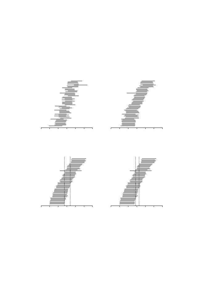
Figure 5.3: Bayesian estimates of government bailout propensities (me-
dian and 80% Bayesian credible intervals of the posterior distribution of

θ).

Democracies are identiﬁed with an open circle.

Model 1

Model 2

AUS 1989

SPN 1977

COL 1982

NZL 1987

ARG 1995

PHI 1998

ECU 1996

MLY 1985

ARG 1989

POL 1992

THA 1983

BUL 1996

TUR 1982

VEN 1994

BRZ 1994

USA 1981

IND 1992

ARG 1980

GHA 1982

NOR 1987

FRA 1994

CHL 1981

PAR 1995

THA 1997

TUR 1994

HUN 1991

CIV 1988

SEN 1988

FIN 1991

SWE 1991

PHI 1983

MEX 1982

JAP 1992

PAN 1988

LAT 1995

URU 1981

SLO 1992

EGY 1991

SLK 1989

KOR 1997

EST 1992

LIT 1995

IND 1997

MLY 1997

CZE 1989

MEX 1994

−3

−2

−1

●

−3

−2

−1

AUS 1989

SPN 1977

COL 1982

NZL 1987

ARG 1995

PHI 1998

ECU 1996

MLY 1985

ARG 1989

POL 1992

THA 1983

BUL 1996

TUR 1982

VEN 1994

BRZ 1994

USA 1981

IND 1992

ARG 1980

GHA 1982

NOR 1987

FRA 1994

CHL 1981

PAR 1995

THA 1997

TUR 1994

HUN 1991

CIV 1988

SEN 1988

FIN 1991

SWE 1991

PHI 1983

MEX 1982

JAP 1992

PAN 1988

LAT 1995

URU 1981

SLO 1992

EGY 1991

SLK 1989

KOR 1997

EST 1992

LIT 1995

IND 1997

MLY 1997

CZE 1989

MEX 1994

●

Model 3

Model 4

−3

−2

−1

AUS 1989

SPN 1977

COL 1982

NZL 1987

ARG 1995

PHI 1998

ECU 1996

MLY 1985

ARG 1989

POL 1992

THA 1983

BUL 1996

TUR 1982

VEN 1994

BRZ 1994

USA 1981

IND 1992

ARG 1980

GHA 1982

NOR 1987

FRA 1994

CHL 1981

PAR 1995

THA 1997

TUR 1994

HUN 1991

CIV 1988

SEN 1988

FIN 1991

SWE 1991

PHI 1983

MEX 1982

JAP 1992

PAN 1988

LAT 1995

URU 1981

SLO 1992

EGY 1991

SLK 1989

KOR 1997

EST 1992

LIT 1995

IND 1997

MLY 1997

CZE 1989

MEX 1994

●

−3

−2

−1

AUS 1989

SPN 1977

COL 1982

NZL 1987

ARG 1995

PHI 1998

ECU 1996

MLY 1985

ARG 1989

POL 1992

THA 1983

BUL 1996

TUR 1982

VEN 1994

BRZ 1994

USA 1981

IND 1992

ARG 1980

GHA 1982

NOR 1987

FRA 1994

CHL 1981

PAR 1995

THA 1997

TUR 1994

HUN 1991

CIV 1988

SEN 1988

FIN 1991

SWE 1991

PHI 1983

MEX 1982

JAP 1992

PAN 1988

LAT 1995

URU 1981

SLO 1992

EGY 1991

SLK 1989

KOR 1997

EST 1992

LIT 1995

IND 1997

MLY 1997

CZE 1989

MEX 1994

●

ote: Governments are arranged from most to least Bailout-prone based on Model 3: Mexico

1994, Czechoslovakia 1989, Malaysia 1997, Indonesia 1997, Lithuania 1995, Estonia 1992,

South Korea 1997, Sri Lanka 1989, Egypt 1991, Slovenia 1992, Uruguay 1981, Latvia 1995,

Panama 1988, Japan 1992, Mexico 1982, Philippines 1983, Sweden 1991, Finland 1991, Senegal

1988, Cˆote d’Ivoire 1988, Hungary 1991, Turkey 1994, Thailand 1997, Paraguay 1995, Chile

1981, France 1994, Norway 1987, Ghana 1982, Argentina 1980, Indonesia 1992, United States

1981, Brazil 1994, Venezuela 1994, Turkey 1982, Bulgaria 1996, Thailand 1983, Poland 1992,

Argentina 1989, Malaysia 1985, Ecuador 1996, Philippines 1998, Argentina 1995, New Zealand

1987, Colombia 1982, Spain 1977, Australia 1989.

110

Curbing Bailouts

items, we do see a clearly deﬁned group of democratic polities in the lower
end of the graph, while non-democratic regimes appear to be plentiful towards
the upper end. These results are encouraging and call for proper estimation
of the e

ﬀect of political regime on bailout propensities. Though one could

use estimated bailout propensities as dependent variables in a regression
framework, it is arguably best to directly assess the e

ﬀect of political regimes

within the IRT model by building a hierarchical model for bailout propensities

θ. In this context, I incorporate information about the political regimes under

which governments face banking crises by assuming that bailout propensities

are a function of democracy. Equation 5.4 incorporates this extension:

∼ N(μ

, 1)

(5.4)

= δ · democracy

The more general model is thus described by Equations 5.1, 5.3, and 5.4.

In this model, the distribution of government-speciﬁc parameters

is condi-

tioned on a “hyperparameter”

, which is itself a function of the political

regime under which governments confront a banking crisis. Parameter

δ cap-

tures the average e

ﬀect of democracy on a government’s bailout propensity.

If democracies enact solutions closer to the Bagehot ideal-type, the posterior
density of

δ should be negative.

The last two columns of Table 5.2 display

estimates of the general model based on two di

ﬀerent indicators of political

regime: Estimates in Model 3 are based on Przeworski et al.’s dichotomous
indicator of democracy-authoritarianism, whereas Model 4 reports estimates
based on a continuous measure of political regime, namely, the Polity IV
index, that takes integer values between –10 and 10.

The basic message conveyed by these models is that, regardless of in-

dicator, political regimes are statistically associated with di

ﬀerent bailout

propensities.

This is most clearly seen in the model based on the dichoto-

mous regime indicator (Model 3), whose coe

ﬃcient is estimated to lie entirely

to the left of 0. In the model based on the dichotomous democracy indicator

(Model 4),

δ can best be interpreted as a diﬀerence of means between the

bailout propensities of democratic and non-democratic governments. This dif-
ference in means is portrayed graphically in the lower-left panel of Figure 5.3:
On the horizontal axis, the point labeled “D” (at

= −0.27) corresponds to

the mean bailout propensity of all democratic regimes, whereas “A” captures
mean propensity among authoritarian regimes (

= 0.38). The average mean

I do not estimate an intercept, consistent with the fact that the democracy indicators are

mean-centered and the prior distribution of

δ is centered at 0. The prior distribution of δ is

normal with mean 0 and precision 0.01, which is not particularly informative given the scale
on which bailout propensity is measured (the scale remains unchanged, as can be seen from
distribution assumptions about

θ in Equation 5.4).

In Rosas (2006), I show that this association holds for a variety of democracy indicators.

Variation in Government Bailout Propensities

111

Table 5.3: Posterior predictive distribution of the implementation of seven

crisis-management policies. Cell entries correspond to the expected frequency

(%) with which each policy is adopted under democracy and non-democracy.

Policy

Democracy

Non-democracy

Asset management

Recapitalization

Explicit guarantees

Regulatory forbearance

Bank liquidity

Debt relief

Deposit freeze

ﬀerence between democracies and non-democracies is −0.65; considering

that the bailout propensity scale has standard deviation 1 by construction, this
di

ﬀerence is far from trivial. Admittedly, the estimated political regime eﬀect

seems muted when we consider a continuous measure of democracy, as in
Model 4. In this case, the posterior distribution of parameter

δ even has some

probability mass to the right of 0. Thus, based on estimates in Model 4, I
calculate the probability that democracies have larger than average bailout
propensities to be about 0.23, which is not a trivial amount. As a consequence,
the e

ﬀect of political regimes on bailout propensities displayed in the lower-

right panel of Figure 5.3 is smaller. Since the democracy indicator used in
column 4 is continuous, points labeled “D” and “A” correspond in this case to
the sample interquartile range of the Polity indicator.

The degree of association between political regime and bailout propen-

sities is put in its proper context once we consider the interaction between
parameters

θ, on the one hand, and the diﬃculty and discrimination parame-

ters

α and β of diﬀerent policy items, on the other. The rightmost panel in

Figure 5.2 portrays interval estimates of predicted probabilities of implemen-
tation of the seven policy issues conditional on the political regime under

which a government confronts a crisis. Though political regimes are conse-

quential in determining the bailout propensity of di

ﬀerent governments, the

low discrimination potential of some items means that the e

ﬀect of democracy

on liquidity, debt relief, and deposit freeze is relatively small. For all other
policy items, political regimes make a huge di

ﬀerence even when we take

into account uncertainty in the estimation of parameters, as Figure 5.2 does.

To see this, notice that despite overlap in the credible intervals of these param-

eters we can still estimate probabilities of policy enactment under alternative

112

Curbing Bailouts

political regimes with relative precision. Table 5.3 summarizes results of a
simulation in which I predict implementation of the seven crisis-management
policies under the two political regimes.

For example, we would expect

democratic governments to implement regulatory forbearance in response
to a banking crisis about half the time (47%), whereas authoritarian regimes

would implement the same policy 3 times out of 4 (74%). Even for policies
with low discrimination parameters, like bank liquidity or debt relief, we still

ﬁnd that democracies implement these policies 2 times out of 5 and 1 time
out of 4, respectively, as opposed to non-democracies, which implement these
policies about 3 times out of 5 and 1 time out of 3. Since the bailout propen-
sities of governments correlate with the ﬁscal cost of restoring solvency to
distressed banking systems, it is arguably cheaper to be a taxpayer under
democratic than under authoritarian regimes.

5.4 Incorporating Information from Recent Bailouts

Consistent with a view of crisis-management policy as a continuum going
from Bagehot to Bailout ideal-types, I estimated IRT models that recover
di

ﬀerences in the bailout propensities of governments from principled analysis

of dichotomous policy indicators. The ancillary parameters of these models
conﬁrm the expectation that not all of these policies are equally likely to
be enacted, i.e., crisis-management policies vary in their degree of political
expediency. Furthermore, inspection of these parameters suggests that large
di

ﬀerences in the bailout propensities of governments may have little impact

on implementation of some of these policies. This ﬁnding should increase
awareness that these policy indicators need to be considered in tandem, lest
one ends placing too much stock on policies that in the end provide too
little information about the underlying bailout propensities of governments.

This ﬁnding also suggests that relaxing the assumption of unidimensional

bailout propensities might be worthwhile; some of the policy items with weak
discrimination parameters may in fact help us separate Bailout from Bagehot
cases if we only allow for a more complex model. I investigate this scenario
in Chapter 6.

The main focus of the analysis, though, was assessment of Proposition 1.

The argument according to which democracies are less likely than authoritar-

ian regimes to bail out insolvent banking systems is plausible, as suggested
by analysis of a sample of 46 government responses to as many banking
crises. Indeed, democratic governments are statistically less bailout-prone

The percentages in Table 5.3 obtain from drawing 100 samples from the joint posterior

distribution of parameters, then substituting them in Equations 5.1, 5.3, and 5.4. The percentage
corresponds to the frequency with which the given policy was implemented (i.e., ˆy

= 1).

Variation in Government Bailout Propensities

113

than authoritarian regimes, and their e

ﬀect on choice of diﬀerent policies

appears to be substantively important as well. This last statement, for which I
provide more support in Chapter 6, might ring hollow given the observation
of recent bank bailouts, particularly in the United States and Great Britain,
the two countries with the longest-running history of democracy on record.

As I mentioned before, the observation of bank bailouts in democracies is

neither extraordinary nor deﬁnitive proof that my argument about the repre-
sentation of taxpayers’ interests in this type of regime is misplaced. However,
reasonable skepticism is warranted about the degree to which these recent
bailouts alter inferences about democratic e

ﬀects. To couch the question in

the vocabulary of Bayesian inference, how does our knowledge about the
e

ﬀects of democracy on bank bailouts change after updating based on these

new data?

To face problems of insolvency and illiquidity, a variety of governments

around the world have recently taken actions to prop up their banking systems.

Though the shape that these interventions will take, the degree of relief that

they will bring to distressed banks, and the changes that they will e

ﬀect on

banking systems remain to be seen, it is possible to carry out a preliminary
assessment based on information available at the time of writing. To guar-
antee a minimum of coherence and comparability, I base this assessment on
the Financial Times (FT) characterization of government responses to the
subprime-mortgage ﬁnancial crisis as of October 17, 2008.

This source

summarizes government decisions along six policy areas in 29 countries that
have been a

ﬀected by the recent ﬁnancial meltdown: liquidity and lending

guarantees, bank deposit guarantees, bank recapitalization, asset purchase,
interest rate moves, and crackdowns on short selling. The ﬁrst four areas in
this list correspond closely to liquidity, explicit guarantees, recapitalization,
and asset management agency; under bank deposit guarantees, furthermore,
this source reports one government, Ukraine, that has enacted a deposit freeze.

This source does not consider debt relief or regulatory forbearance as policy

categories, which does not necessarily mean that these policies have not been
implemented; however, for the purpose of this preliminary exercise, I consider
these policies as missing values. I use the FT information to construct di-
chotomous indicators for ﬁve of the seven policies I have thus far considered
and I allow previous estimates of item parameters to be updated based on
these data. Admittedly, the correspondence between the FT characterization

http://www.ft.com/

, last accessed on December 12, 2008. The 29 countries are: Aus-

tralia, Austria, Belgium, China, Denmark, Finland, France, Germany, Great Britain, Greece,
Hungary, Iceland, Indonesia, Ireland, Japan, South Korea, New Zealand, Netherlands, Norway,
Portugal, Qatar, Russia, Saudi Arabia, Spain, Sweden, Switzerland, United Arab Emirates,
United States, and the Ukraine. I code China, Qatar, Russia, Saudi Arabia, and United Arab
Emirates as non-democracies.

114

Curbing Bailouts

of policy and the coding decisions of Honohan and Klingebiel (2000) is not
perfect, but these preliminary data nonetheless allow a further empirical test
of the existence of a democratic advantage.

To update knowledge about the inﬂuence of democracy on bailout propen-

sities, I re-estimate the IRT speciﬁcation that corresponds to Model 3 in

Table 5.2. Since all relevant knowledge about e

ﬀect parameters that we can

get from the original sample of N

= 46 cases is already contained in the

posterior distributions reported in that model, we need only use these as prior
distributions in a new round of Bayesian updating.

Thus, I use the posterior

distributions reported in Model 3 (Table 5.2) as a summary of the state of
knowledge about bailout propensities. For example, the democratic e

ﬀect

parameter

δ is normally distributed with mean −0.324 and standard deviation

.192; this is the prior information for the democratic eﬀect parameter whose

distribution I update based on new data.

After incorporating the new information, the updated results mostly sug-

gest changes in item di

ﬃculty parameters; recall that these parameters reﬂect

how common di

ﬀerent types of policies are, and may provide a clue as to the

political expediency of these policies.

Among discrimination parameters,

the new information leads to changes that are hardly consequential: asset
management, recapitalization, and guarantee are still the policies most likely
to be implemented by governments with high bailout propensity, whereas
deposit freeze and liquidity still show parameters that are substantively minute.

The main parameter of interest is

δ, corresponding to the democratic eﬀect.

The posterior distribution of this parameter, based on the new information, is

centered on

−0.267, with standard deviation 0.165. This suggests a slightly

reduced e

ﬀect, but still one that leads credence to the proposition that demo-

cratic governments are less likely to engage in bailouts. This e

ﬀect continues

I code a policy as present whenever FT mentions its implementation, with one exception: I

only code explicit guarantees as implemented if the policy extends existing deposit insurance
schemes to all deposits in the banking system. Due to lack of comparable data, I eschew
information on interest rate moves and short selling crackdowns (these are outright prohibitions
to engage in the practice of “shorting,” or selling stock that the seller holds on loan at the time of
the transaction).

Bayes theorem guarantees that the “ﬁnal” posterior distributions based on this two-stage

updating method will be identical to the posterior distributions obtained by re-running all models
on an expanded sample of N

= 46 + 29 (DeGroot and Schervish 2002, 72–73). This attractive

property of Bayesian estimation implies that we can continue to update our knowledge about the
e

ﬀect of democracy on bank bailouts as new information continues to appear in the months to

come.

Mean and standard deviation of the posterior distribution of di

ﬃculty parameters are:

.80 ± 0.23;

: 0

.59 ± 0.24;

: 0

.37 ± 0.22;

−0.22 ± 0.15;

: 0

.64 ± 0.16. The

corresponding statistics for discrimination parameters are:

: 0

.80 ± 0.23; β

: 0

.59 ± 0.24;

: 0

.37 ± 0.22; β

−0.22 ± 0.15; β

: 0

.64 ± 0.16. Since I add no new information about debt

relief or forbearance, knowledge about these parameters is not updated.

Variation in Government Bailout Propensities

115

to obtain even after considering evidence from mostly democratic countries
that have implemented bailout policies to prop up their banking systems.

Be this as it may, it is not in general possible to provide a causal inter-

pretation of the political regime e

ﬀect δ when this parameter is estimated

based on observational data. As I argued before, the original sample of 46
government responses is broadly representative of the universe of registered
banking crises between 1975 and 2000, but the mechanism of assignment
of governments to treatment (democracy) and control (non-democracy) is
obviously not known. Under these circumstances, causal interpretation of co-
e

ﬃcient δ is only possible under very stringent assumptions about ignorability

of the treatment assignment and appropriateness of model speciﬁcation. In
Chapter 6, I make e

ﬀorts to substantiate a causal interpretation of the eﬀect

of democratic regimes on bank bailout policies.

Political Regimes and Bailout Propensities

This chapter contributes several necessary extensions to the analysis presented

in Chapter 5. The purpose of these extensions is twofold: First, I intend to
throw further light on the process that leads governments to implement bank
bailouts. Second, and more importantly, I plan to convince the reader that
the restraining e

ﬀect of democratic regimes holds after controlling for other

obvious determinants of government policy choice, and after correcting for
covariate imbalance and potential endogeneity of political regimes. In short,
my goal is to build a case for a causal, rather than strictly correlational,
interpretation of the e

ﬀects unveiled in Chapter 5.

To do so, I divide the chapter in four sections. Section 6.1 considers

alternative explanatory factors that might impinge on the propensity of gov-
ernments to bail out insolvent banks. One such factor stands out as an
important potential confounder, namely, the level of autonomy of a nation’s
central bank. A second factor—the existence of crony links between bankers
and politicians—should be an important predictor of government bailout
propensities, but the argument in Chapter 3 leads me to consider this factor as
a direct consequence of the level of democracy in a country. In short, I believe
that extensive crony networks are endogenous to democratic representation
and accountability. Cronyism in this account is a “post-treatment” variable
that should not be controlled for in an analysis of the causal e

ﬀects of political

regime, lest the e

ﬀect of democracy be estimated with bias. Even then, my

view of cronyism as endogenous to democracy may be incorrect. Therefore,
I consider initially an indicator of corruption among the set of desirable
controls in a regression setup. Aside from these two factors, I consider co-
variates such as the degree of capital account openness of a country, its level
of economic development and inequality, and the relative importance of the
domestic banking sector as a crucial link in a country’s payments system in
order to approximate the stringent assumption of conditional independence.

116

Political Regimes and Bailout Propensities

117

Sections 6.2 and 6.3 include these controls in the IRT model speciﬁcations

ﬁrst presented in Chapter 5, ﬁrst without and then with corrections for covari-
ate imbalance and endogeneity. The main message of these sections is that
political regimes matter even after making allowances for the observational
nature of the sample. Finally, Section 6.4 considers a two-dimensional exten-
sion to the basic unidimensional IRT model of Chapter 5. Section 6.4 thus
explores whether governments make “disjoint” choices along two di

ﬀerent

policy dimensions, one corresponding to bank solvency considerations, the
other to liquidity concerns. I do so because preliminary results in Chapter 5
suggest that policies to redress solvency and liquidity problems may not
necessarily correlate. It follows from this ﬁnding that political regimes may
only a

ﬀect one set of policies—i.e., solvency or liquidity policies—rather

than both of them. I conclude that political regimes have little e

ﬀect, if any,

on liquidity policies.

6.1 Alternative Explanations

The theoretical argument in Chapter 3 points to the existence of a democratic

ﬀect in the way in which governments respond to banking crises. The

mechanism behind this e

ﬀect is governmental anticipation of the policy

preferences of the median voter, which leads to more conservative closure
rules in the event of a banking crisis.

In Chapter 5, I estimate a political regime parameter (

δ) in a regression-

like framework and posit that its size and sign are consistent with Propo-
sition 1. This interpretation is not strictly correct: For

δ to reﬂect a true

democratic e

ﬀect, its estimation would require random assignment conditions

that can only be approached, at best, through experimental manipulation. In
the absence of true random assignment in an experimental setting, a causal in-
terpretation of

δ depends on very stringent assumptions about the process that

generated assignment of governments into the democracy and non-democracy
categories, assumptions that can only be approximated with careful modeling
choices. The ﬁrst and perhaps most important of these assumptions is condi-
tional independence, also known as ignorability of the treatment assignment
or selection on observables. The most obvious way to think about conditional
independence is as a requirement to control for confounding covariates that
may be associated both with political regimes and bailout propensities.

Needless to say, building an exhaustive catalog of all such potential con-

founding covariates is well-nigh impossible. However, political economists
have studied a variety of factors that may be consequential in understanding
government bailout propensities. More importantly, the theoretical argument
explored in Chapter 3 points to several obvious confounding factors. Previous

118

Curbing Bailouts

theoretical knowledge suggests that central bank independence, importance
of the domestic banking sector, the level of economic openness of a country,
and its level of economic development should be controlled for to approximate
conditional independence. I consider each of these potential confounders in
the following sections.

6.1.1 Central Bank Independence

The theoretical argument in Chapter 3 is premised on the assumption that

governments are not constrained in their ability to provide loans to distressed
banks upon observation of large liquidity shocks. In other words, I assume that
politicians control the levers of monetary policy. However, this assumption is
not entirely tenable in countries where central banks are autonomous from
political pressures. More problematically, many polities have moved in
recent decades towards the adoption of charters that secure independence
for central banks and allow them to pursue monetary stability with minimal
political meddling (Maxﬁeld 1997). It is well understood that politicians
may be tempted to rely on easy money in hard economic times (Kydland
and Prescott 1977; Sargent and Wallace 1975); hence the relevance of policy
advice to get politicians’ hands o

ﬀ monetary policy. Indeed, the proposition

that institutionally-autonomous central banks are less likely to produce high
bouts of inﬂation has received ample empirical conﬁrmation in observational
studies (Cukierman 1992; Cukierman, Miller and Neyapti 2002; Cukierman,

Webb and Neyapti 1992; Desai, Olofsgård and Yousef 2003; Franzese 1999;

Grilli, Masciandaro and Tabellini 1991).

The stabilizing e

ﬀect of autonomous central banks is relevant in an anal-

ysis of bank bailouts because these institutions are also called to perform
the function of lending of last resort (cf. Bagehot 1873; Goodhart and Illing
2002). From the point of view of the monetary authority, banking crises
may present a stark choice between an expansive policy to aid illiquid banks
and conservative use of the monetary tool to preserve price stability. Even
independent central banks could decide, however, to bail out banks rather
than preserve the value of the national currency. After all, institutional inde-
pendence from political pressures only guarantees that politicians will not
control the money supply; it does not necessarily mean that central bankers
will always err on the side of preserving price stability. Still, because of
legal stipulations to pursue low inﬂation that are often found in central bank
charters, independent central bankers should be less likely, all else constant,
to act as overly generous lenders of last resort to the banking system during a
crisis, let alone to accommodate ﬁscal expansion to bail out banks. Inasmuch
as central bank autonomy entails tighter monetary policy, it should also curtail
a politician’s ability to carry out bank bailouts.

Political Regimes and Bailout Propensities

119

Despite its likely e

ﬀect on bailout propensities, central bank autonomy

should be considered a relevant confounding variable only if it is also associ-
ated with political regimes. Evidence and theory suggesting elective a

ﬃnities

between democracies and autonomous central banks are less plentiful. Part of
the problem is that the literature on the political determinants of institutional
variation in the status of central banks has focused largely on advanced mar-
ket economies, which are by-and-large democratic. For example, Bernhard
argues that variation in intraparty or intracoalitional conﬂicts explains incen-
tives to delegate monetary policy to independent central banks, an argument
he substantiates by analyzing central bank reform in advanced democratic
regimes (Bernhard 2002). Relatedly, some contributions consider the e

ﬀect

of veto players on the adoption (Hallerberg 2002) and e

ﬀectiveness (Keefer

and Stasavage 2002, 2003) of di

ﬀerent monetary policy arrangements. An

implication of these arguments is that adoption of central bank independence
may be related to political regimes, as democracies are more likely to count

with checks-and-balance mechanisms captured by the notion of veto players.

Perhaps Boylan (2001) and Broz (2002) present the clearest theoretical ar-
guments substantiating the possibility of a correlation between central bank
status and political regime. Boylan contends that authoritarian regimes that
carry out deep market-oriented economic reform may provide autonomy to
the monetary authority in anticipation of transition to democracy. By doing so,
market-friendly dictators secure their economic legacy by limiting the ability
of proﬂigate democratic governments to spend their way into ﬁscal crises. By
this account, independent central banks ought to be over-represented among
democracies with recent authoritarian pasts. Broz (2002) also suggests that
political regimes and central bank independence may be correlated. In his
argument, countries signal commitment to a low-inﬂation monetary policy
by choosing a ﬁxed exchange rate regime (a transparent signal) or central
bank independence (an “opaque” commitment technology). In democracies,
the political process is itself transparent, and so resorting to central bank
independence signals commitment; autocracies instead can only resort to
ﬁxed exchange rates. Democracies can take advantage of central bank inde-
pendence as a commitment mechanism because they are transparent regimes
Other arguments about central bank independence discount the possibility
of a

ﬃnities between political regimes and central bank status. For example,

Maxﬁeld (1997) considers the adoption of central bank independence among
middle-income economies to be a consequence of a country’s need for inter-
national credit and investment, regardless of political regime; in her account,
central bank independence sends a credible signal of credit-worthiness to
international investors.

Be this as it may, the institutional status of central banks is perhaps the

most important confounding variable in my analysis, so regardless of its

120

Curbing Bailouts

theoretical links with political regimes I include it as a covariate. I resort to
the index of legal central bank independence created by Cukierman, Webb
and Neyapti (1992) and updated by Cukierman, Miller and Neyapti (2002)
and Polillo and Guill´en (2005) as an indicator of the institutional status of the
monetary authority. The correlation between Przeworski et al.’s dichotomous
regime score and the index of legal central bank independence based on 39
full observations is 0.25, which indeed suggests that democratic politicians
tend to have less inﬂuence on the conduct of monetary policy.

6.1.2 Economic Development and Inequality

It is important to control for the e

ﬀect of economic variables for two reasons.

First and foremost, my argument about the constraining e

ﬀects of democracy

is premised on the idea that di

ﬀerent economic structures aﬀect the probability

that governments will engage in bailouts. Recall that the argument in Chap-
ter 3 suggests that bailouts are relatively more onerous to the median voter
in unequal societies. Therefore, inequality should be negatively associated

with a government’s bailout propensity. In principle, this e

ﬀect should also be

seen with regards to level of economic development. As we saw in Chapter 3,
a government’s closure rule becomes more conservative (i.e., the government

will have lower bailout propensity) as the average level of economic well-

being in society increases. The e

ﬀect of economic development, however,

occurs only through the spread parameter

σ in the Pareto distribution that I

use to approximate patterns of economic inequality. Therefore, after control-
ling for inequality, a country’s level of economic development may have little
e

ﬀect on its government’s bailout propensity.

Second, recent advances in political economy suggest that both level of

economic development and economic inequality may a

ﬀect a society’s oppor-

tunities to develop a sustainable democratic regime. In the case of economic
development, an old debate that in its most recent incarnation can be traced
back to modernization theory concerns the links between democracy and

wealth. Some argue that democracies are simply more likely to survive under

conditions of economic a

ﬄuence (Przeworski et al. 2000), whereas others

provide evidence that wealth directly engenders democracy (Boix and Stokes
2003). In either case, it is evident that richer countries are more likely to have
democratic political regimes than poorer countries, so in fact there is a high
correlation between these two variables. When it comes to economic inequal-
ity, democracies might be more unlikely to emerge and survive in economies

with grave patterns of inequality (Acemoglu and Robinson 2005; Boix 2003).

Underlying this insight is the proposition that the policy preferences of the
median voter in unequal societies are for greater redistribution from the very
rich. Anticipating that these preferences will be decisive under democratic

Political Regimes and Bailout Propensities

121

rule, economic elites oppose transition to a more open political regime; in-
stead, they might be more willing to accept democracy if the median voter
prefers less redistribution, as happens in principle in egalitarian societies.

In other words, it is unlikely that political regimes are independent of

patterns of economic inequality and development. Inequality and develop-
ment are likely to be correlated with the main independent variable,

and as

argued in Chapter 3 they should also a

ﬀect bailout propensities. If we were

not to control for these two variables, we might mistakenly attribute part of
their inﬂuence on bailout propensity to a country’s political regime. I use
the real per capita GDP of a country (log scale) as an indicator of level of
development; for economic inequality, I use Gini indices from the United
Nations University’s World Income Inequality Database, as corrected by
Desai, Olofsgård and Yousef (2003).

6.1.3 Crony Capitalism

The theoretical importance that many scholars grant to crony capitalism as

a factor that explains bank bailouts is undeniable. As reviewed in Chap-
ter 1, several scholars have studied the links between politicians and en-
trepreneurs

/bankers, and conclude that these are economically consequen-

tial. At the ﬁrm level, Faccio (2006) and Faccio, Masulis and McConnell

(2006) study the performance of ﬁrms that count politicians among their large

shareholders or as board members and compares it with the performance of
non-connected ﬁrms. Faccio does not assume explicitly the existence of any
quid pro quo in the relationship between politicians and entrepreneurs, but
her research ﬁnds that political connectedness provides ﬁrms with better debt
ﬁnancing, higher tax beneﬁts, and larger market power. Politically-connected
ﬁrms are also more ine

ﬃcient, as they tend to generate lower returns-on-

equity, lower market-to-book ratios, and lower stock prices. More tellingly,
politically-connected ﬁrms are more likely to be bailed out in case of ﬁnancial
distress. In the realm of banking, Bongini, Claessens and Ferri (2001) ﬁnd
that banks with crony links were more likely to su

ﬀer ﬁnancial distress based

on bank-level data from the East Asian ﬁnancial crisis, even though crony
links were not signiﬁcant predictors of bailouts. There is also some evidence
that government-owned banks are routinely used to bolster political fortunes.
Dinc¸ (2005) ﬁnds that government-owned banks in emerging markets increase
their lending in election years compared to private banks and Khwaja and
Mian (2005) explore loan-level data from Pakistan to discover that public
banks make larger loans to connected ﬁrms, that returns on these assets are

The sample correlations between inequality and GDP per capita, on the one hand, and the

dichotomous democracy score, on the other, are

−0.086 and 0.495. Sample correlations with the

continuous Polity IV score are

−0.139 and 0.556, respectively.

122

Curbing Bailouts

lower, that connected ﬁrms are more likely to default, and that recovery rates
conditional on default are lower for connected ﬁrms. Moreover, stronger
politicians (based on information about their electoral prowess) are more
likely to get larger loans.

Crony capitalism should also be related to a country’s political regime,

a conclusion I arrive at in my theoretical analysis. In Chapter 3, politicians
in democratic regimes purport to implement the policy preferences of the
median voter. Since these preferences are for less onerous bailouts, politicians
strive to reduce the impact of ﬁnancial distress on taxpayers, and they do so
by, among other things, limiting the extent of crony links with entrepreneurs.
Incidentally, Haber (2002a) provides a theory about crony capitalism that
starts from di

ﬀerent assumptions but reaches similar implications. In his

theory, democracy and cronyism are functional equivalents in that either of
these factors gives credibility to the ruler’s commitment not to expropriate
investments. The di

ﬀerence between these factors is that where democracy

makes this commitment credible by creating checks on arbitrary rule, crony-
ism solves the commitment problem by allowing the ruler to share in the
rents created by entrepreneurial action, thus reducing the ruler’s temptation
to expropriate.

In any case, I expect democracy and cronyism to be negatively correlated,

but I also believe with Haber that there is a strong causal link ﬂowing from
political regime to cronyism. Consequently, any proxy for crony capitalism
should be appropriately considered a “post-treatment variable” according to
the argument laid out in Chapter 3. As such, its inclusion is not advisable
in a model that purports to estimate causal e

ﬀects of political regimes. The

inclusion of post-treatment variables in a regression framework works at
cross-purposes with the inclusion of pre-treatment variables. Whereas con-
trolling for pre-treatment variables like economic development or economic
inequality helps one approximate the ideal condition of comparing “like”
units, introducing a proxy for a post-treatment variable all but guarantees that

“treated” and “control” units will be fundamentally di

ﬀerent (Gelman and

Hill 2007, 188–190). If my theoretical argument is correct, including a crony
capitalism variable in the regression analysis would radically change the
interpretation of the political regime coe

ﬃcient. In this case, the coeﬃcient

of democracy would represent a di

ﬀerence in bailout propensities among

observations that vary along the political regime dimension, but also along the
crony capitalism dimension. Be this as it may, my theoretical framework may
be mistaken in assuming that crony capitalism is endogenous to democracy.
If in fact cronyism is not endogenous to democracy, the empirical correlation
between indicators of political regime and cronyism would mandate inclusion
of the latter among the set of controlling factors in a regression setup. To
cover all bases, I estimate models with and without an indicator of crony

Political Regimes and Bailout Propensities

123

capitalism. As I show below, the estimated coe

ﬃcient of political regime

on bailout propensity is substantively smaller when including the crony cap-
italism indicator, as is to be expected, but in general not too di

ﬀerent from

estimates of the regime e

ﬀect in the absence of a crony capitalism indicator.

Kang (2002) notes in his study on East Asia how di

ﬃcult it is to measure

intrinsic features of crony capitalism. In contrast with him, I do consider that
indicators of corruption provide a reasonable approximation to the measure-
ment of cronyism at the country level. Admittedly, cronyism and corruption
are not synonyms, but it is reasonable to expect that where corruption is low
the chances are also low that politicians, bankers, and entrepreneurs will
be consistently enmeshed in the kind of crony arrangements suggested in
Chapter 3. I build an indicator of relative lack of corruption, transparency,
from commonly employed data (Knack and Keefer 1998; Transparency Inter-
national 2002). I expect the ensuing transparency measure to be negatively
associated with bailout propensity.

6.1.4 Other Controls

To approximate conditional independence, it is important to control for at

least two other factors: capital openness and importance of the domestic bank-
ing sector. I consider the possibility, hinted at but not considered explicitly in
Chapter 3, that the optimal closure rule may be a function of the importance
of banks within a country’s ﬁnancial sector. Where ﬁnancial markets are pri-
marily organized around banks, then bank closures threaten severe economic
disruptions as the ensuing credit crunch threatens entrepreneurial projects.
Undoubtedly, some of these projects should be terminated, especially if they
contributed to bank insolvency, but bank closures also derail viable projects.
Politicians may ﬁnd it too costly to terminate banks if their failure threatens
high negative externalities. In other words, I acknowledge that redressing
bank insolvency at minimum public cost might entail postponing the exit of
insolvent banks from the banking system. To control for this factor, I include
the ratio of total deposits in the banking system to gross domestic product

(Beck, Demirg¨uc¸-Kunt and Levine 1999). Deposit share is a proxy for the

relative importance of banks as intermediaries within a nation’s ﬁnancial
system.

Domestic institutions that hinder cronyism are not the only potential con-

straints on a politician’s decision to bail out banks. Instead, international
factors impinge upon domestic policy-making. In an era of global integration
of capital and goods markets, the ability of politicians to carry out independent

Treisman (2000) shows that TI and ICRG (Knack and Keefer 1998) indices are very highly

correlated. Hence, I standardize these two measures to a common 1–10 metric and use their
average as an indicator of transparency.

124

Curbing Bailouts

public policies can be constrained by the possibility of capital ﬂight (Andrews

1994; Cooper 1968; Oatley 1999). Though opening up a nation’s borders to

capital ﬂows and increased trade opportunities improves a country’s access
to cheaper credit and allows specialization close to comparative advantage,
it might also mean foregoing the use of Keynesian tools of demand manage-
ment. As Obstfeld (1998) argues, globalization has the beneﬁcial side-e

ﬀect

of disciplining governments, forcing them into a path of sustainable budgets
and price stability. With respect to bank bailouts, globalization might exert
a similar downward pressure on ﬁscal proﬂigacy. Politicians may choose
policies closer to Bagehot to the extent that their countries are more thor-
oughly integrated into the world economy through capital markets. Therefore,
I include an indicator of capital openness as a further control (Chinn and Ito
2002).

As argued before, one can potentially think of a host of factors that

might determine a government’s bailout propensity and that may correlate

with political regimes. However, omitted variables pose a threat to causal

interpretation (a) when they correlate with the dependent variable, and (b)

when they are causally prior to the independent variable whose causal impact

one aims to gauge, in this case regime type. This is the case for all controls
discussed in the previous sections. I also considered several other covariates
in alternative speciﬁcations, which are reported in an exploratory paper (cf.
Rosas 2006). Among these, I included a dummy for the existence of a
stand-by agreement with the IMF on the starting year of a banking crisis,
an indicator of bank concentration, the market share of foreign banks, the
micro- vs. macro-economic origin of banking crises, and the country’s
degree of trade openness. Though some of these indicators were signiﬁcant
predictors of bailout propensity, they did not alter the estimated e

ﬀect of

political regime in a substantive way. Furthermore, I could not ﬁnd theoretical
arguments that would allow me to construe these indicators as pre-treatment
factors associated with democracy, which explains my preference for more
parsimonious model speciﬁcations.

6.2 Controlling for Observable Predictors

Table A.2.2 in the Appendix contains summary information about all indi-

cators used in the analysis.

The control variables discussed in the previous

As Table A.2.2 makes clear, there are missing values in some covariates. Throughout the

book, I deal with missing values in independent variables in a principled way. First, I obtain
multiple imputations of missing values in a Bayesian MCMC context under the assumption of
random missingness (Van Buuren and Oudshoorn 2000). I then estimate all models based on ﬁve
complete datasets, which contain as many imputations for each missing value. Reported estimates
are based on a combination of the ﬁve resulting samples from the posterior distribution; using

Political Regimes and Bailout Propensities

125

sections are added as predictors of government bailout propensities, that is,

= δ

· democracy

+ δ

· central bank

+ · · · + δ

· deposit share

(6.1)

The hierarchical speciﬁcation of Equation 6.1 adds a series of control variables

to the basic setup of Equation 5.4. In other words, the new speciﬁcation
recognizes that governments in the sample di

ﬀer along dimensions other than

just their political regimes; some of these dimensions may be consequential
in understanding the bailout propensities of governments as they react to
banking crises. I estimate four versions of this model.

Table 6.1 displays

Bayesian estimates of e

ﬀect parameters δ; estimates of item discrimination

(

β) and diﬃculty (α) parameters are omitted for the sake of space, but in all

cases are very similar to those reported in Table 5.2.

Models 1 and 3 in Table 6.1 conﬁrm the negative association between

continuous and dichotomous political regime indicators, on the one hand, and
bailout propensity, on the other, that I had uncovered before, this time after
controlling for theoretically-relevant factors and the “post-treatment” trans-
parency indicator. In fact, estimates of the e

ﬀect parameters of democracy

in both models are about similar in magnitude to the ones in Chapter 5. In
the case of the dichotomous indicator (Model 3), the posterior distribution
of the e

ﬀect parameter for democracy is clearly centered away from 0 and

on the negative orthant (its 95% credible interval is –1.106, –0.199); when
switching to the continuous Polity IV score (Model 1), the 95% credible
interval for the e

ﬀect parameter still straddles 0, as was the case in Chap-

ter 5, though most probability mass still appears to the left of 0. It is also
noteworthy that estimated coe

ﬃcients for other control variables are signed

according to expectations. Especially in Model 3, the posterior distributions
of coe

ﬃcients on central bank independence (95% CI: –0.686, 0.109) and

income inequality (95% CI: –0.774, 0.069) have little probability mass to
the right of zero, suggesting that countries with high levels of central bank
autonomy and high levels of economic inequality are less prone to engage
in bailout policies, all else constant. The negative sign on the central bank
coe

ﬃcient is consistent with accumulated theoretical knowledge about the

this procedure, one can appropriately factor uncertainty derived from the multiple imputation
process into coe

ﬃcient estimates. Missing values in dependent variables are still imputed as

a by-product of the MCMC sampling process (see fn. 7 in Chapter 5). This process can be
regarded as an iterative multiple imputation procedure that properly reﬂects uncertainty due to
missing values (see Gelman et al. 2004, 519–520).

These models are identiﬁed using restrictions similar to those employed in Chapter 5. In

particular, I avoid rotational invariance by assuming a priori that discrimination parameters can
only take on non-negative values. As in Chapter 5, all indicators are standardized; since they
have mean 0 and the prior distribution of

θ is also centered at 0, I do not estimate an intercept.

The prior distribution on each coe

ﬃcient δ is N(0, 0.001), a diﬀuse and rather uninformative

prior.

126

Curbing Bailouts

Table 6.1: Bayesian estimation of covariate coe

ﬃcients (δ). The point esti-

mate is the median of the parameter’s posterior density (standard deviation
of the posterior density in parentheses). Models 1 and 2 are based on the
continuous Polity IV democracy indicator; Models 3 and 4 are based on the
dichotomous regime indicator in Przeworski et al. (2000).

Model 1

Model 2

Model 3

Model 4

Democracy

−0.239

−0.251

−0.609

−0.534

.254)

.238)

.254)

.262)

Central bank

−0.146

−0.179

−0.274

−0.257

.211)

.221)

.243)

.226)

GDP per capita

.184

−0.108

.389

.031

.379)

.281)

.402)

.288)

Income inequality

−0.311

−0.445

−0.351

−0.502

.244)

.225)

.260)

.251)

Capital openness

−0.064

−0.023

−0.154

−0.101

.263)

.251)

.260)

.277)

Deposit share

−0.041

.044

−0.010

.022

.251)

.226)

.266)

.228)

Transparency

−0.210

−0.203

.389)

.388)

DIC

376

.70

374

.90

376

.10

374

.20

.99

.69

.50

.77

restraining e

ﬀect of autonomy of the monetary authority. The coeﬃcient on

income inequality is in line with predictions ﬂowing from Chapter 3 about
the unwillingness of politicians to have generous closure rules in countries

where the median voter is relatively poorer.

Other control variables have coe

ﬃcients that are not entirely distinguish-

able from 0, but are in most cases signed in the right direction. In the case
of GDP per capita, my theoretical expectation was either a nil e

ﬀect or a

negative e

ﬀect. Recall from Chapter 3 that the “location” parameter of a

country’s economic distribution (

μ) drops out of the politician’s calculus as

she entertains whether to support an illiquid bank or not. Given that we
identify this parameter with the overall level of wealth of a country, this
theoretical result would lead one to expect a nil e

ﬀect. However, given the

speciﬁc assumptions I made about the theoretical distribution of income in an
economy, the “spread” parameter (

σ corresponds more closely to economic

Political Regimes and Bailout Propensities

127

inequality) also a

ﬀects overall levels of wealth (higher values of σ correspond

to higher average wealth). In this interpretation, we would then expect a
negative association between GDP per capita and bailout propensity. Either

way, the point estimate for GDP per capita shifts signs depending on whether

transparency is also controlled for, an artifact of high sample correlation
between these two variables; the posterior distribution of this parameter is
extremely wide and leaves ample probability mass to the left and right of
0. For all purposes, I conclude that the coe

ﬃcient of GDP per capita is not

distinguishable from 0. The same argument leads me to disregard deposit
share as a relevant predictor of bailout propensity.

The coe

ﬃcients on transparency and capital openness are signed accord-

ing to expectations—they are both negative, suggesting that more transparent
and open economies are less likely to su

ﬀer bailout-prone governments—but

again their coe

ﬃcients have posterior distributions with wide standard devia-

tions that straddle 0. Incidentally, excluding transparency from the analysis,
as I do in Models 2 and 4, has discernible e

ﬀects on the estimates of GDP

per capita but not on the political regime coe

ﬃcients, which remain largely

unchanged. Recall that the rationale for the exclusion of transparency is the
post-treatment character of crony capitalism in my theoretical account of
bank bailouts.

Models 1 through 4 conﬁrm that democratic regimes are associated with

lower bailout propensities, even after accounting for potential confounders.

The mechanism linking political regimes to bank bailouts is anticipation of

the policy preferences of the median voter. The negative sign on income in-
equality is consistent with this interpretation; after all, the median voter in an
economically inegalitarian society carries relatively higher costs and enjoys
relatively lower beneﬁts from banks that are restored to solvency using taxpay-
ers’ money. This evidence leads me to believe that the posited mechanism is
indeed responsible for the degree of association between political regimes and
bailout propensities. Further evidence comes from dissecting democracy into
two of its main characteristics. Indeed, while I have emphasized representa-
tion of the policy preferences of the median voter

/taxpayer—which is enabled

by accountability of democratic politicians to the electorate—as the relevant
mechanism, democratic regimes are also characterized by strong systems of
checks-and-balances that may limit policy response. The positive association
between bailout propensities and political regimes may be the consequence
of democratic checks-and-balances rather than democratic accountability.

To distinguish the e

ﬀects of these diﬀerent features of democracy on

bailouts, I decompose the Polity IV score into its three separate “concept
variables” and use two of these to proxy for the accountability and checks-and-
balances mechanisms of democracy. The relevant sub-indices are described
as “the extent of institutional constraints on the decision-making powers of

128

Curbing Bailouts

the chief executive” (excons) and “the openness of executive recruitment”

(exrec). Though correspondences are far from perfect, excons embodies the

idea of veto points, whereas exrec corresponds to the ease with which voters
can replace the holder of executive power. In a speciﬁcation identical to
that of Models 2 and 4, the posterior distribution of excons is centered on
−0.14 ± 0.24 (median ± SD); when I replace exrec for excons in this model,
the posterior distribution lies more clearly on the negative orthant and is
centered on

−0.36 (±0.24). Finally, I resort to the checks2 indicator from

the Database of Political Institutions, which is a more obvious proxy for
the number of veto points or legislative checks on executive behavior. The
posterior distribution of checks2 is centered on 0

.21 (±0.20), which suggests

that, if anything, more veto points are conducive to higher bailout propensities.

These alternative estimates suggest that to the degree that political regimes

are good predictors of bailout propensities, the transmission mechanism is
more likely to be electoral accountability than checks-and-balances.

6.3 A Causal Interpretation of Regime E

ﬀects

Controlling for observed confounders is not the only obstacle in the way of a
causal interpretation of the e

ﬀect parameter of democracy. The analysis in

this chapter is based on observational data, and therefore one must proceed

with caution to reach valid causal inferences about the e

ﬀects of political

regimes on bailout propensities. I explore issues of covariate imbalance and
non-ignorable treatment assignment in this section.

To motivate the discus-

sion, consider the distribution of control variables across democracies and
non-democracies based on the dichotomous indicator of political regimes (Ta-
ble 6.2). Consistent with observed relations among wealth, income inequality,
and political regimes in the contemporary world, we see that democracies in
the sample are on average richer and have ﬂatter income distributions than
non-democratic regimes. Furthermore, and also consistent with previous the-
oretical knowledge, the democratic regimes in the sample tend to have higher
transparency scores; they also have larger measures of deposit share, which is
likely a consequence of the higher degree of development among democratic
regimes. Instead, the di

ﬀerence between mean central bank independence

scores across democratic and non-democratic regimes seems trivial.

Naturally, this lack of balance in the sample distribution of covariates

provides an important rationale for including them as control variables in the
bailout propensity models. After all, we know that researchers cannot assign

These are problems that plague the search for causal e

ﬀects regardless of the inferential

framework that researchers adopt; that is, they need to be addressed in Bayesian analysis as
much as in a frequentist setup.

Political Regimes and Bailout Propensities

129

Table 6.2: Sample means of control variables across democratic and non-

democratic regimes, along with percent improvement in balance based on
matched data

% Balance

Non-democracy

Democracy

improvement

Central bank autonomy

.37

.32

100

.00

GDP per capita (log)

.40

.10

.86

Income inequality

.21

.19

.94

Capital openness

.48

.59

−7.35

Transparency

.48

.34

.28

Deposit share

.31

.36

.45

Propensity score

.32

.38

.17

political regimes randomly to countries, a situation that would automatically
guarantee conditional independence across units. But even after controlling
for these factors, the condition of covariate imbalance across political regimes
poses a more subtle quandary to our ability to provide a causal interpretation
of the regime e

ﬀect. Because we tend to observe democratic regimes among

countries that are richer, have more egalitarian income distributions, and more
transparent business environments, there exists a real risk that the estimated
e

ﬀect of democracy on bailout propensity may be driven preponderantly

by assumptions about the functional form of the model. In other words,

we may not have enough data points corresponding to democratic regimes

in poor, unequal, and corrupt settings on which to base an estimate of the
average regime e

ﬀect; in the absence of informative data, this estimate will

be determined solely by the assumption of linearity of bailout propensities

with respect to the e

ﬀect parameter of democracy.

In order to assess the causal impact of political regimes we would like to

observe paired governments identical in all respects except for their political
regime. In this ideal setup, we would be closer to truly estimating the average
causal e

ﬀect of democracy on bailout propositions. Though a perfect pairing

of democratic and non-democratic regimes is not possible, it is possible to
limit the sample to a reduced set of observations that are closely “matched.”
By doing so, we can approximate conditions of randomization of observed

130

Curbing Bailouts

Figure 6.1: Propensity scores of democracies and non-democracies. Black
dots are unmatched democracies, gray dots correspond to observations outside
the region of common support.

Propensity scores

Democracies Non

−

democracies

●

● ●

●

● ●

●

covariates across treatment and control groups.

To this e

ﬀect, I use the tech-

nique of nearest neighbor matching based on propensity scores. In essence, I
estimate propensity scores for each observation based on a logistic regression
of political regime on the six relevant control variables of Table 6.2. Note that
these “propensity scores” are not the same as the government “bailout propen-
sities” shown in Figure 5.3. The propensity scores are the ﬁtted probabilities
derived from the logistic regression and consequently vary between 0 and 1,

with higher numbers corresponding to observations that are more likely to be

predicted as democratic regimes. Finally, each non-democratic regime in the
sample is matched to the one democratic regime with the closest propensity
score; matching proceeds until all non-democracies are matched to one and
only one democracy.

Note ﬁnally that the matching exercise is not based on

information about the dependent variable (i.e., the policy items). In building
a matched dataset, ignoring values of the dependent variable guarantees that
no information on outcomes determines which observations go into treatment
and control groups, and thus approximates conditions of an experimental
design.

Figure 6.1 provides a graphical illustration of how matching renders a

more balanced sample of democracies and non-democracies. The graph plots

Cf. Ho, Imai, King and Stuart (2007a); King and Zeng (2006); Rosenbaum and Rubin

(1983).

I use the MatchIt software of Ho, Imai, King and Stuart (2007b). Because of missing

observations among some of the covariates in these logit models, I impute missing values before
proceeding with propensity score matching. In practice, then, I carry out the matching exercise
on ﬁve imputed datasets, identical in all respects except in the values of missing observations
that were imputed.

Political Regimes and Bailout Propensities

131

the forty-six democratic and non-democratic governments on the vertical
axis (jittered for display purposes) against each government’s propensity
score. Because the distribution of political regimes is not random with
respect to control variables, the propensity scores of democracies tend to be
higher than the propensity scores of non-democracies. After matching, some
of the democratic regimes—corresponding to the black dots in the lower-
right corner—are dropped from the analysis, which leaves 19 democracies
matched with 19 non-democracies. The eight democratic governments that
are dropped from the analysis are Finland 1991, Hungary 1991, Japan 1992,
Korea 1997, New Zealand 1987, Norway 1987, Spain 1977, and Sweden

1991. This list of unmatched democracies conﬁrms, for example, the outlier

character of the Scandinavian democracies (Finland and Sweden have Gini
scores that are more than one standard deviation below the sample mean),
but some of these other countries are “unique” in other ways. As can be
gleaned from Table 6.2, balance among covariates is much improved; the

“% balance improvement” statistic is a measure of the distance between the

sample distribution of covariates across democracies and non-democracies
before and after matching. Except for capital openness, which is slightly
more unbalanced after than before matching, there are notable improvements
in the similarity of cases across political regimes when analysis is restricted
to the matched sample. Thus, the sample of matched observations achieves
maximum balance on covariates and keeps as many observations as possible
in the analysis.

Parameter estimates based on the reduced matched sample of 38 govern-

ments appear in Table 6.3 (item parameter estimates, not shown, are similar to
those in Table 5.2). The estimated political regime e

ﬀects are slightly smaller

than those based on the full sample (Table 6.1), but they are of similar magni-
tude (point estimates are –0.52 and –0.50, 90% credible intervals are –0.98 to

–0.10 in Model 5 and –0.93 to –0.11 in Model 6). Model 5 includes relevant

controls and conﬁrms that the negative coe

ﬃcient estimate for democracy is

not overtly dependent on the functional form of the model. Model 6 omits
controls and instead estimates a coe

ﬃcient for the propensity score itself. It

should in principle be su

ﬃcient to include propensity scores as the relevant

control, because these measures already contain all possible information
about covariate imbalance (Rosenbaum and Rubin 1983). However, the main
condition for propensity scores to be a valid summary of covariates is that
they are based on the “true” propensity model, which needless to say is an
unveriﬁable assumption. Be this as it may, comparison of the coe

ﬃcient

estimates for democracy in Models 5 and 6 conﬁrms that not much is lost
by substituting control covariates with the propensity score; this ﬁnding will
come handy in Section 6.4.

Returning to Figure 6.1, we can see that propensity score matching still

able

6.3:

Bayesian

estimation

ernment-le

parameters

(δ

)

based

exclusi

ely

matc

hed

(Models

5–6)

common

support

(Models

7–8)

cases,

and

instrumental

variables

two-sta

least

squar

ession

(Models

9–10).

Point

estimate

the

median

the

parameter’

posterior

density

(standard

viation

the

posterior

density).

Matched

observ

ations

Common

support

2SLS

Model

Democr

acy

−

523

−

503

−

487

−

437

−

282

−

141

.270)

.249)

.303)

.239)

.110)

.149)

Centr

bank

−

549

−

837

−

074

−

049

.299)

.356)

.095)

.096)

GDP

per

capita

192

362

−

015

−

060

.288)

.345)

.108)

.109)

Income

inequality

−

699

−

942

−

170

−

157

.314)

.393)

.098)

.100)

Capital

openness

−

261

−

113

−

003

025

.279)

.340)

.101)

.099)

Deposit

shar

034

022

041

.246)

.248)

.102)

.100)

opensity

scor

167

211

.228)

.234)

DIC

301

255

256

.09

220

.29

.43

.73

.31

Political Regimes and Bailout Propensities

133

leaves some imbalance in the distribution of propensity scores. Even worse,
the graph suggests that the overlap of propensity scores between democracies
and non-democracies is far from perfect. Lack of complete overlap means
that there are democracies in the sample which do not have a “counterfactual”
observation, i.e., another observation alike in all respects but with a non-
democratic regime. In Figure 6.1 I have identiﬁed six further observations,
shown as gray dots, that lie outside the common support of propensity scores.

These include four democracies (Argentina 1989, Australia 1989, Brazil,

1994, and France 1994) and two authoritarian regimes (Indonesia 1997 and

Senegal 1988). When these are dropped from the analysis, the remaining
sample is no longer perfectly matched (there are ﬁfteen democracies and
seventeen non-democracies), but is now based on observations with common
support on propensity scores. Parameter estimates based on the “common
support” sample with 32 observations appear in Models 7 and 8. Again,
the estimated political regime e

ﬀects are lower than in larger samples, but

still remain within the same order of magnitude (point estimates are –0.49
and –0.44, 90% CI from

−1.02 to −0.05 in Model 7 and −0.85 to −0.06

in Model 8). Based on these results, we can conclude that lack of balance
among covariates—which bedevils many estimates of the e

ﬀects of political

regimes in realms other than banking policy because of the a

ﬃnities among

wealth, equality, and democracy—is of no great consequence in this sample.

Consequently, for the remainder of the chapter, I will inspect information
from the full sample of 46 observations.

Having concluded that covariate imbalance is not problematic, I now

turn to the second quandary—the assumption of ignorability of the treatment
assignment —which turns out to be more consequential. In part, I have
already taken steps to approximate this assumption by including observed
covariates in the models of bailout propensity. Taking this step guarantees
that the e

ﬀect of democracy is not vulnerable to the problem of selection on

observables. However, there may well be other unobserved factors—the real
extent of insolvency, the severity of an exogenous shock, or the lobbying
power of bank shareholders, for example—that may correlate with political
regimes and a

ﬀect the ability of governments to deal with banking crises, thus

ﬀecting their bailout propensities. Though I have been careful to include

as controls all factors that relate theoretically to political regime and bailout
propensity, the basic inability to randomize treatment in observational studies
means that one can never be sure that the e

ﬀect of democracy is not biased by

unobserved omitted variables. Keefer (2007, p. 632) for example wonders if
the reduced propensity of democracies to engage in bailouts “could be driven
by the possibility that precrisis ﬁnancial policies are di

ﬀerent in democracies

and autocracies, a

ﬀecting the probability that they experience crises or the

nature of those crises and, as a consequence, their policy response once crisis

134

Curbing Bailouts

occurs.” There are several alternative ways of alleviating this problem in
applied research. The approach I follow here is to provide an instrumental-
variables estimate of the e

ﬀect of democracy on bailout propensities based on

two-stage least squares analysis.

In order to perform this estimation, it is necessary to count with a valid

instrument for political regime. Recently, there have been a variety of attempts
to interpret coe

ﬃcients in observational political economy studies in a causal

manner; it is little wonder then that several instruments of democracy have
been recently proposed.

I considered oil exports, British colonial heritage,

constitutional age of a country, number of prior transitions to democracy, and
coastline length as potential instruments. Behind each of these instrumental
variables there is a theoretical account that substantiates the assumption
of ignorability of the instrument. Unfortunately, none of these potential
instruments correlated highly with democratic status in the sample, therefore
failing the basic condition of non-zero association between instrument and
treatment variable. In the end, I resorted to the average level of regional
democracy as an instrument for political regime. The correlation between
political regime and the proposed instrument is 0.556.

Aside from this criterion of relevance, the validity of instrumental vari-

ables estimation hinges on two critical assumptions, namely, monotonicity
and exclusion restriction. To assess the degree of verisimilitude of these
assumptions, consider the rationale for employing regional democracy as an
instrument for a country’s regime type. We know empirically that authori-
tarian countries are more likely to transit to democracy if a majority of their
neighbors are democratic (Gleditsch and Ward 2006). The “di

ﬀusion eﬀect”

of democracies may operate through a variety of mechanisms. Gleditsch and

Ward (2006), for example, consider the possibility that the democratization of

neighboring countries may change the regional distribution of power and

/or

the preferences of politicians and societal actors in an authoritarian regime.
In this context, the assumption of monotonicity implies that a country in a
region with high levels of democracy is at least as likely to be a democracy as
it would be were it located in a region with low levels of democracy. This as-
sumption is eminently plausible given ample evidence about the mechanisms
behind di

ﬀusion of democracy. The second assumption, exclusion restriction,

implies that a government’s bailout propensity is not a

ﬀected by regional

democracy after controlling for its own political regime. In other words, any
e

ﬀect that regional democracy may have on bailout propensities is assumed

to occur exclusively through its impact on regime itself. This assumption

would be violated, for example, if democratic regimes in the vicinity of a

ﬁnancially-troubled democracy tended to lend a hand by providing funds

See inter alia Keefer (2007); Persson and Tabellini (2003); Przeworski et al. (2000).

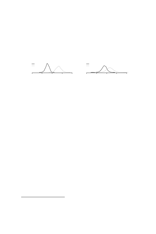
Political Regimes and Bailout Propensities

135

Figure 6.2: Posterior predictive distribution of bailout propensity scores for
democratic and non-democratic regimes. The panel on the left is based on
Bayesian regression estimates, the panel on the right on Bayesian IV-2SLS
estimates.

IRT

IV-2SLS

Bailout propensity

−1.0

−0.5

0.0

0.5

1.0

D
A

Bailout propensity

−1.0

−0.5

0.0

0.5

1.0

D
A

to bail out banks. Whereas support to manage banking crises may be avail-
able from international ﬁnancial institutions or even other large countries, it
does not seem plausible that neighboring countries would coordinate for this
purpose.

Before discussing the instrumental variables estimate of the democracy

ﬀect, one further caveat is in order. The estimates presented in Models

9 and 10 are not based on the extended IRT model I have discussed so
far. To facilitate estimation, the dependent variable in these models is the
point estimate of government bailout propensities derived from Model 4
in Table 5.2. These point estimates provide my best guess regarding the
underlying propensity of each government to engage in bailouts, and are based
on information from the seven crisis management policies and the political
regime of each government. It is no wonder, then, that the Bayesian regression
estimate of democracy in Model 9 is negative and clearly bounded away from
0, with a 90% credible interval from –0.47 to –0.11. I provide the instrumental
variables estimate of the e

ﬀect of democracy on bailout propensity in Model

10. I arrive at this estimate through two-stage least squares analysis in a

Bayesian framework (WinBugs code is in Appendix A.3.3).

The instrumental variables estimate invites greater caution in gauging

the empirical validity of Proposition 1. In fact, the IV estimate in Model 10
is about half the size of the regression estimate of Model 9 and has wider
standard error (0.39, with 90% CI from –0.44 to 0.1). Figure 6.2 provides
an illustration of these e

ﬀects. These plots graph the posterior predictive

The exclusion restriction is testable in an overidentiﬁed model. In other words, it would be

necessary to include a second instrument to test this assumption. Given the paucity of relevant
instruments, I am not able to carry out statistical tests of the validity of the exclusion restriction.

136

Curbing Bailouts

distributions of bailout propensity scores based on Models 9 (left plot) and

10 (right plot), while holding all other covariates ﬁxed at their mean sample

values. Based on the posterior predictive distributions in the left plot, I
estimate the probability that autocracies have lower bailout propensities than
democracies to be less than 0.01.

According to this model, democracies have average bailout scores of

–0.23, whereas an average non-democratic regime would have a score of 0.33.

In contrast, based on the IV model I estimate the probability that autocracies
may have lower bailout propensity scores than democracies to be about 0.156,
i.e., there is a non-negligible probability, though still relatively small, that
authoritarian regimes are more contained than democracies in approaching
crisis management. Based on the IV estimate, democracies (non-democracies)
have an average bailout score of –0.12 (0.17).

Before wrapping up this section, it is important to recall what instrumental

variables analysis allows us to say about the e

ﬀect of instrumented predictors.

An observational study can only inform about the average treatment e

ﬀect for

units whose treatment can be construed as having been somehow manipulated

(Angrist, Imbens and Rubin 1996). The literature on causal inference refers

to this as the local average treatment e

ﬀect. In this case, the IV estimate is

not based on countries that would be democratic even if surrounded by au-
thoritarian countries (“always compliers” in the parlance of causal inference)
nor on countries that would be authoritarian even if surrounded by democratic
countries (“never compliers”).

The IV estimate, as it were, is the average e

ﬀect on bailout propensities of

authoritarian regimes that could be compelled to transit to democracy by the
sheer fact of being surrounded by democracies (“induced democracies”) and
of democratic regimes that could turn into non-democracies if surrounded by
this type of country (“induced autocracies”). Instrumental variables analysis
therefore provides consistent estimates of a more limited notion of causal
e

ﬀect than would obtain in a real experimental setting where treatment and

control status could be assigned randomly.

I thus conclude with a more cautious note about the empirical validity of

Proposition 1. If we construe the IV local average treatment e

ﬀect estimates

as a lower bound—and the substantively larger estimates obtained in Models

1 through 9 as an upper bound—on the true e

ﬀect of democracy on bailout

propensities, then we can say that democracies are much less likely than non-
democracies to engage in crisis-management policies closer to the ideal-type
of Bailout. However, the substantive e

ﬀects of political regime on policy

output, though positive, may not be as large as those originally reported in

Table 5.3.

Political Regimes and Bailout Propensities

137

6.4 Distinct Solvency and Liquidity Bailout Propensities

Three of the seven policies inspected in Chapter 5—liquidity provision, de-

posit freeze, and debt relief —showed low capacity to discriminate among
Bagehot and Bailout governments, as evinced by discrimination parameters
that were not clearly centered away from 0. In a one-dimensional setting,
these ﬁndings suggest that such policies provide little information about gov-
ernment bailout propensities beyond what is already provided by their sample
frequency. However, these are consequential and costly policies meant to
postpone the exit of distressed banks with immediate liquidity problems and
that may very well be insolvent, as analyzed in Chapter 3. For this reason
alone, it is not plausible that governments implement these policies haphaz-
ardly, more or less independently of their bailout propensities. Instead, the
lack of discrimination power of these items along a single dimension may be
due to the existence of a second policy dimension that has so far remained
untapped.

To build intuition about the substantive policy content of this hypothesized

second dimension, consider that liquidity provision, deposit freeze, and debt
relief are policies that aim to control bank cash-ﬂows. When banks face
deposit runs, liquidity provision and debt relief keep them from having to
liquidate assets in order to meet cash outﬂows. The ﬁrst policy does so by
providing ample support from the central bank, the latter by giving bank
debtors the wherewithal to avoid defaults on their loans. Deposit freezes
achieve the same objective through di

ﬀerent means: By prohibiting cash

outﬂows, governments remove the burden of asset liquidation from banks,
buying time to rebuild their portfolios and restructure loan payments without
facing immediate pressure from jittery depositors. Note ﬁnally that these
three policies achieve the same objective—i.e., preventing asset liquidation to
meet deposit runs—through antithetical means. In other words, these policies
are almost perfect substitutes. Indeed, if deposits are frozen, it is not really
necessary to provide discount loans to banks. For this reason, we seldom see
implementation of liquidity provision or debt relief when a deposit freeze is
in place. Out of the 46 observations in the sample, 41 governments enacted at
least one of these three policies, but only 5 implemented deposit freeze along

with either debt relief or liquidity provision, and only three governments

implemented all three of these policies concurrently. I refer to these cash-ﬂow
management actions as liquidity policies.

Because Bagehot’s maxim of lending on good collateral to solvent banks

implies providing ample support to some ﬁnancial intermediaries, one may
be tempted to construe implementation of these policies, particularly liquidity
provision, as a signal of a more restrained bailout propensity. However,
Honohan and Klingebiel (2000) make it clear that they code governments

138

Curbing Bailouts

as having engaged in liquidity provision, debt relief, and deposit freeze only
if they hold these policies in place for a long period (see Table 5.1). In the
case of debt relief, governments get a “1” if they extend a helping hand to
large corporate borrowers. In no case are these policies coded “1” as a result
of a limited “market-upholding” intervention by a Bagehot policy-maker.
Consequently, implementation of these policies suggests policy action closer
to the Bailout ideal-type.

To sum up, it is understandable that the three liquidity policies do not

help discriminate Bagehot from Bailout governments when one assumes the
existence of a single policy dimension. But should we expect liquidity and
solvency dimensions to be correlated? As discussed in Chapters 1 and 3,
policies to redress solvency and liquidity need not correlate. On the one hand,
systemic bank insolvency need not produce large panic deposit runs if, for
instance, depositors are protected by a credible system of deposit insurance.
On the other hand, liquidity problems in a banking system need not be the
consequence of generalized bank insolvency. For this reason, if solvency and
liquidity policy dimensions were close to uncorrelated, a one-dimensional
model would fail to capture variation in government propensity to engage in
bailout practices along both solvency and liquidity fronts.

To explore the possibility that liquidity policies are indeed informative

about government types but not reducible to a single Bagehot-Bailout un-
derlying dimension, I expand the IRT model considered so far to admit two
di

ﬀerent dimensions, θ

and

, that capture bailout propensities in the realms

of solvency and liquidity, respectively. The relevant change to Equation 5.3
appears in Equation 6.2:

, j

= Φ(θ

, j

+ θ

, j

− α

)

(6.2)

As can be seen from Equation 6.2, introducing a second dimension in-

creases the number of parameters to estimate and complicates identiﬁcation
of the model. With two underlying dimensions, the identiﬁcation problems
described in Chapter 5 become more insidious, as there are now two di

ﬀerent

sources of rotational and scaling invariance.

It is thus necessary to impose

additional constraints on the two-dimensional model to achieve identiﬁcation.

To do so, I place “spike” priors on some item discrimination parameters

in either dimension 1 or 2. This decision is informed both by theory and by
results from the one-dimensional ﬁt. Thus, the discrimination parameters

for liquidity provision, debt relief, and deposit freeze are assumed to be 0

To see how this extension compounds identiﬁcation problems, consider that, once recovered,

the two dimensions can be multiplied by (1,1), (–1,1), (1,–1), or (–1,–1), and this would not
change the rank-order of governments’ bailout propensities at all. In other words, the two-
dimensional

Θ space can be rotated in 2 × 2 diﬀerent ways (Jackman 2001).

Political Regimes and Bailout Propensities

139

along the ﬁrst dimension, whereas the remaining policy items are assumed to
take on positive values. Along the second dimension, I stipulate that asset
management, recapitalization, and explicit guarantees have

β = 0; in addition,

the discrimination parameter of liquidity provision is constrained to be posi-
tive to ensure that higher scores on the second dimension correspond to higher
bailout propensities. Consider again the substantive meaning of these restric-
tions: I am e

ﬀectively assuming that asset management, recapitalization, and

explicit guarantees provide information exclusively about a government’s
propensity to address bank solvency problems by engaging in bailouts. This
is in line with the evidence reviewed in Chapter 4, where these policies were
shown to promote the restoration of solvency to distressed banking systems in

Argentina and Mexico. I am also assuming that liquidity provision, debt relief,

and deposit freeze provide information about a government’s propensity to
provide liquidity assistance, but not to address solvency problems. Finally, I
allow regulatory forbearance to provide information about both dimensions.

This is consistent with results from the one-dimensional model, where the

discrimination parameter of this policy was positive, but substantively small.

The solution I adopt overidentiﬁes the model, in the sense that estimation

could in principle be carried out with slightly less severe restrictions, but
avoids imposing direct restrictions on governments’ bailout propensities. Fur-
thermore, with sample size unchanged at 46 observations, these additional
constraints allow data to be informative about a relatively smaller number of
parameters.

Table 6.4 displays summary information about the item parameters of a

two-dimensional IRT model. Due to the multiplicity of parameters to esti-
mate, I include only three government-level covariates in this speciﬁcation:
democracy, central bank and propensity score. The latter indicator is included
in lieu of all other control variables in an e

ﬀort to approximate the assumption

of conditional independence. The central bank indicator is included here on
account of the accumulated knowledge about the monetary e

ﬀects of central

bank independence reviewed in Section 6.1.1. Based on the central bank
autonomy literature, I expect this indicator to correlate negatively with the
liquidity dimension. As for the democracy indicator, I am again interested
in testing the validity of Proposition 1 with regard to separate solvency and
liquidity dimensions. The theoretical argument in Chapter 3 was premised
on the assumption that the government controlled monetary policy. Flowing
from this assumption, one would expect that democracy would also correlate
negatively with liquidity in the two-dimensional model. However, govern-
ments may be limited in their ability to make decisions regarding cash-ﬂow
management in the presence of a politically-autonomous central bank. If this
is indeed the case, then the e

ﬀect of democracy on a government’s liquidity

score would be essentially nil.

140

Curbing Bailouts

Table 6.4: Bayesian estimation of Bagehot-Bailout policy discrimination (

β)

and government-level (

δ) parameters. The point estimate is the median of the

parameter’s posterior density (standard deviation of the posterior density in
parentheses).

Solvency

Liquidity

dimension

Democracy

−0.535

.063

.261)

.301)

Central bank

−0.186

−0.468

.222)

.332)

Propensity score

−0.247

.265

.251)

.303)

.228

.392)

.199

.340)

.171

.414)

F B

.510

.259

.323)

.413)

.934

.474)

.490

.349)

−0.942

.473)

DIC

352.98

57.11

= liquidity, D = debt relief, AM = asset management agency,

= recapitalization, G = explicit guarantees, F = deposit freeze,

= forbearance

Before commenting on the results, one indication that the one- and two-

dimensional models are appropriately identiﬁed, even under di

ﬀerent para-

metric restrictions, is that both yield similar posterior distributions for the

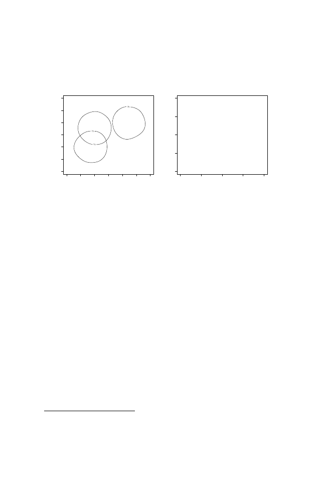
Political Regimes and Bailout Propensities

141

Figure 6.3: Bailout propensity scores of democratic and non-democratic
regimes along solvency and liquidity dimensions

−3

−2

−1

−

123

Solvency

Liquidity

Argentina 1995

Colombia 1982

Mexico 1994

−2

−1

−

Solvency

Liquidity

●

seven item di

ﬃculty parameters.

Naturally, these posterior distributions are

narrower in the one-dimensional model, as that model requires estimation
of a lower number of parameters. Thus, the one- and two-dimensional mod-
els reveal very similar information regarding the di

ﬃculty of implementing

policies to address banking crises.

The posterior distribution of discrimination parameters conﬁrms that the

second dimension captures government propensities to engage in measures
to alleviate liquidity problems in the banking system. Obviously, since the
parameter on liquidity provision was purposefully constrained to be positive,
I cannot invoke its magnitude and direction as corroborating the nature of
the second latent propensity scale. Note however that deposit freeze has a
negative discrimination parameter along the second dimension whereas debt
relief has positive discrimination parameter, conﬁrming indeed that freezing
deposits is a policy that does not tend to occur simultaneously with policies
to relieve bank debtors or with excessively generous central bank lending. As
for regulatory forbearance, whose coe

ﬃcient was not constrained a priori,

parameter estimates suggest that this policy discriminates mostly along the
solvency dimension. The posterior distribution of its discrimination parameter
on the liquidity dimension is positive, but wide enough to straddle zero.

Conﬁrming the narrative of Chapter 4, the left panel of Figure 6.3 portrays

75% credible intervals for the two-dimensional bailout propensities of the

Point estimates (

±SD) for diﬃculty parameters follow: α

= 0.36 (±0.30), α

= 0.91

(

±0.32), α

= 0.23 (±0.28), α

F B

= −0.45 (±0.25), α

= −0.04 (±0.26), α

= 0.80 (±0.26),

= 0.31 (±0.27).

142

Curbing Bailouts

Argentine and Mexican governments during the Tequila crises (Colombia

1982 is also plotted for comparison). Consistent with knowledge about policy

responses to these crises, the Argentine government of Carlos Sa´ul Menem
scores very low on both bailout dimensions, whereas Ernesto Zedillo’s is one
of the most bailout-prone governments in the sample. Indeed, I estimate the
probability that this government is the most bailout-prone in terms of solvency
support to be about 0.15; in terms of liquidity support, this probability falls
to 0.069. Instead, the chances that Argentina 1995 is the least bailout-prone
government along these two dimensions are 0.11 and 0.067, respectively.

This model throws further light onto potential di

ﬀerences between democ-

racies and non-democracies in the use of policy tools to manage banking
crises. In this regard, the right panel of Figure 6.3 plots point estimates of
bailout scores for the forty-six observations in the sample along the solvency
and liquidity dimensions (incidentally, the correlation between the two di-
mensions is only 0.03, i.e., these dimensions are orthogonal for practical
purposes). The plot distinguishes between democratic regimes (open circles)
and non-democracies (solid circles). Consistent with results in Table 6.4,
there is no readily distinguishable di

ﬀerence in the spread of democracies and

authoritarian regimes along the liquidity dimension; we do see however that
democracies tend to cluster on the lower ranges of the solvency dimension.

But how do these di

ﬀerences between political regimes translate into

predicted probabilities of observing di

ﬀerent types of policy interventions

to manage banking crises? Table 6.5 suggests how di

ﬀerent combinations

of political regimes and central bank status yield rather di

ﬀerent predictions

about the crisis-management policies that we would expect to see. Based on
the estimates of Table 6.4, we would expect a democratic government in a
country where an independent central bank is in control of monetary policy
to engage in regulatory forbearance about half the time (52%). Democratic
regimes are a lot less likely to generously nourish banks back to solvency
at the expense of taxpayers. For example, even where central banks are
not independent from the political process, democratic governments are
reluctant to establish public asset management corporations, which more
often than not end up failing to recover more than a fraction of the face value
of non-performing loans. Democratic governments are also less likely to
issue explicit deposit guarantees over and above existing deposit insurance
schemes (about 3 out of 10 times); they are also very unlikely to recapitalize
banks using public funds (about 1 in 10 times). The chances that democratic
governments will engage in this kind of policy are even lower where policy
action is constrained by an independent central bank.

With the possible exception of deposit freezes, which are a bit less com-

mon under democracies, political regimes have very little impact on liquidity
policies. This is of course consistent with the e

ﬀect parameter of democracy

Political Regimes and Bailout Propensities

143

Table 6.5: Posterior predictive distribution of the implementation of seven

crisis-management policies. Cell entries correspond to the expected frequency

(%) with which each policy is adopted under di

ﬀerent combinations of politi-

cal regime and central bank independence (25

and 75

sample percentiles

of central bank independence).

Democracy

Non-democracy

Low CBI

Asset management

Recapitalization

Explicit guarantees

Regulatory forbearance

Bank liquidity

Debt relief

Deposit freeze

High CBI

Asset management

Recapitalization

Explicit guarantees

Regulatory forbearance

Bank liquidity

Debt relief

Deposit freeze

in Table 6.4, which is basically centered on 0. The existence of an indepen-
dent central bank forces democratic and non-democratic governments alike to
enact deposit freezes about half the time (deposit freezes are far less common

when central banks are not autonomous). Governments of either stripe resort

to debt relief rather sparingly (never more than 1 out of 3 times); this is
the one policy where central bank status does not seem to have much of an
e

ﬀect. Instead, the impact of central bank autonomy appears to be substantial

when it comes to bank liquidity: In the simulation, independent central banks

engage in liquidity support 4 out of 10 times; non-autonomous central banks
provide liquidity support 6 out of 10 times.

6.5 Concluding Remarks

Though the status of monetary policy-making is tangential to my theory of

bank bailouts, the analysis in this chapter suggests that autonomous central
banks have the potential to limit the extent to which taxpayers share in the

144

Curbing Bailouts

burden of ﬁnancial insolvency. Independent central banks may or may not be
reluctant to play the Bagehot script of lending at a discount on good collateral,
but they deﬁnitely appear to be reluctant to sink large amounts of money for
long periods of time into illiquid banking systems. Even then, the evidence
inspected in Chapters 5 and 6 is not inconsistent with Proposition 1—that
is, governments in democratic regimes are less likely to implement generous
bailout policies in response to banking crises—even after taking into account
the constraining e

ﬀect of central bank autonomy. This basic result survives

the inclusion of control variables and corrections for covariate imbalance.
In contrast, the instrumental variables estimate of the political regime e

ﬀect

and the two-dimensional model of liquidity and solvency bailout propensities
invite more caution in assessing regime e

ﬀects. Though the instrumental

variables estimate still suggests the existence of a democratic e

ﬀect, this

ﬀect is more muted than what obtains in models where we assume strict

ignorability of political regime assignment. Similarly, the two-dimensional
model of policy implementation suggests that democratic e

ﬀects may be

circumscribed to policies that aim to redress insolvency, rather than to those
that alleviate liquidity pressures on banks. The latter type of policies are likely
to be determined more by institutional limits on the conduct of monetary
policy—speciﬁcally, by the degree of political autonomy of the central bank—
than by any limits voters may place on socializing the costs of banking crises
in democratic regimes.

Political Regimes and Banking Crises

The theory developed in Chapter 3 suggests that the salutary e

ﬀects of democ-

racy do not stop at limiting ﬁnancial loss-sharing with taxpayers after the
beginning of a banking crisis. Instead, rational forward-looking entrepreneurs
and bankers should be able to anticipate that democratic governments have
limited freedom to engage in onerous bailouts in bad times. This realization
should lead them to take on lower risks in their investment and lending deci-
sions. Furthermore, politicians in democratic governments understand that
electoral accountability constrains their ability to pass on the costs of adjust-
ment to taxpayers, and will therefore choose not to develop extended crony
networks. As suggested by Propositions 2 and 3, both of these e

ﬀects work

in the direction of preventing ﬁnancial distress under democratic regimes.

These propositions are at odds with alternative accounts of the e

ﬀect

of democratic politics on banking crises. As Keefer (2007, 617) argues,
government incentives to enact strict prudential regulation of bank portfolios
are weak, regardless of political regime, “given the often long time lags
between weak regulation and crisis, and the rarity of crisis.” Keefer correctly
points out that banking crises are relatively infrequent, and goes on to suggest
that the infrequency of crises, concurrent with the long lags between weak
regulation and crisis, mean that elected and non-elected governments alike

will lack incentives to invest in strict prudential regulation. In Keefer’s

account, political regimes may not exert a systematic e

ﬀect on the choice of

patterns of prudential regulation of banks. Evidently, this does not mean that
banking regulation is unimportant in understanding banking crises, only that
regulatory structures may not be systematically traced back to di

ﬀerences in

political regime.

In contrast, my explanation emphasizes the credibility of the commitment

not to (excessively) share losses derived from bank insolvency with taxpayers
as the mechanism through which democracies limit ﬁnancial distress. This

145

146

Curbing Bailouts

mechanism is independent of a country’s structure of prudential regulation
of banks. Because I believe this is a strong mechanism that prevents the
most onerous bank bailouts, I also expect it to have an e

ﬀect on measures

of ﬁnancial distress. In addition, if politicians under democratic regimes
understood that regulatory inaction increases the probability of banking crises,
they might actually have incentives to initiate regulatory reforms conducive
to minimize these risks. This alternative mechanism would only add to the
direct e

ﬀect of electoral accountability on banking outcomes, thus reinforcing

the total e

ﬀect of the credible commitment to minimize sharing of ﬁnancial

burden in a democracy. I insist though that the political choice of regulatory
frameworks and the credibility imparted to “no bailout” rules by the electoral
need to consider taxpayer preferences are two distinct mechanisms; the
second mechanism should exert inﬂuence on the behavior of economic actors
independently of regulatory frameworks.

Recall from Chapter 3 that both the probability of bank failure and the

amount of risk taken by entrepreneurs are lower under democratic than under
non-democratic regimes (Figure 3.5), though this e

ﬀect tends to become

muted as the signal about future endstates becomes clearer. I argue that these
theoretical constructs have an empirical correlate in the degree of ﬁnancial
distress of banking systems. If my theory about electoral accountability has
explanatory purchase, ﬁnancial distress should be driven down in democratic
regimes, or at the very least remain constant across regimes; in no case should

we see that democracies are more prone on average to ﬁnancial distress than

non-democracies. I corroborate the degree of association between political
regimes and ﬁnancial distress through a two-pronged strategy. Because acute
ﬁnancial distress occasionally leads to outright banking crises, I make use of
available crisis indicators to estimate the incidence of distress under di

ﬀerent

types of political regimes (Section 7.1).

Banking crises do not exhaust all instances of ﬁnancial distress, however,

so I extend this analysis to consider an alternative indicator built on balance-
sheet accounting ratios measured at the bank system level (Section 7.2). In
the absence of an aggregate-level indicator of market-value net worth, which

would be the most appropriate indicator of overall ﬁnancial solvency in a

banking system, the accounting ratio I consider is a measure of aggregate
book-value net worth. This second indicator of ﬁnancial distress should be
positively correlated with democratic regimes, suggesting that democratic
regimes indeed exert a salutary e

ﬀect on the levels of ﬁnancial solvency of

banking systems. None of these empirical indicators of ﬁnancial distress
in banking systems is perfect—measurements of social phenomena seldom
are—but analyzing indicators that proxy for di

ﬀerent aspects of ﬁnancial

distress increases conﬁdence in inferences about the empirical association
between banking crises and political regimes.

Political Regimes and Banking Crises

147

7.1 Expert Assessments of Banking Crises

In this section, I use expert scores of banking crises to estimate the probability
of failure, and hence levels of ﬁnancial distress, of banking systems across
political regimes. Recall from Chapter 3 that the probability of failure is
marginally higher under non-democratic regimes when the signal about future
endstates is uninformative (q

= 0.5). As the signal about future endstates

becomes clearer, the e

ﬀect of democracy on the probability of failure becomes

less pronounced. Consequently, one would expect, at a minimum, that there

would be no di

ﬀerence in the incidence of banking crises across regime

types. I refer to this as the weak interpretation of political regime e

ﬀects. At

a maximum, we should see the incidence of banking crises to be reduced
under democratic regimes; this is a strong interpretation of regime e

ﬀects.

This testable implication of the argument in Chapter 3 would be deﬁnitely

invalidated if we were to ﬁnd that the probability of failure is actually higher
under democratic regimes.

From the mid-1990s onwards, policy experts have published assessments

of banking crises around the world.

These datasets o

ﬀer information aggre-

gated at the country

/year level, and are often coded dichotomously, though

the dataset I employ includes three categories, as discussed below. In terms
of geographic and temporal coverage, the broadest and most recently updated
e

ﬀort is the World Bank Database of Banking Crises (Caprio et al. 2005),

which identiﬁes the occurrence of banking crises based on a template set by

Lindgren, Garc´ıa and Saal (1996). Basically, this template considers observa-
tion of four di

ﬀerent types of events as evidence that a systemic banking crisis

has occurred in country i in year t. These events are (i) generalized depositor
runs on banks, (ii) accumulation of non-performing loans in excess of 10% of
bank assets, (iii) government assistance to banks through suspension of ﬁnan-
cial activities (e.g., bank holidays or deposit freezes), and (iv) government
support to banks through policies with ﬁscal costs that exceed 2% of GDP.

These four criteria constitute an exhaustive list of “things that can go wrong”

during a banking crisis. More importantly, these criteria allow recognition of
banking crises even in environments where ﬁnancial distress may not trigger
all of these economic behaviors. In other words, any one of these four events
signals the occurrence of a banking crisis. Policy experts need to use various
criteria to identify banking crises because of variation in institutional settings
and accounting rules across countries. For example, it is possible that a
banking system is under severe ﬁnancial strain without necessarily su

ﬀering

Caprio and Klingebiel (1997); Demirg¨uc¸-Kunt and Detragiache (2000); Dziobek and

Pazarbasioglu (1999); Glick and Hutchison (1999); Kaminsky and Reinhart (1999); Lindgren,
Garc´ıa and Saal (1996). See Frydl (1999) and Eichengreen and Arteta (2002) for comparative
analysis of some of these datasets.

148

Curbing Bailouts

generalized deposit runs. In such cases, generalized bank insolvency cannot
be inferred from deposit runs, but it will be fathomed from the behavior of
authorities or depositors. Thus, the four criteria are complementary: the ﬁrst
two criteria—bank runs and accumulation of bad loans—pick up instances of
banking trouble that may or may not have prompted government action but
have already caused changes in depositor or borrower behavior and should
consequently be recognized as outright banking crises, whereas the two latter
criteria—bank holidays and government support—capture events that may
or may not prompt changes in the behavior of economic actors but conﬁrm
that governments have already taken steps to contain ﬁnancial distress. The
complementarity of di

ﬀerent criteria is an undeniable advantage of expert

scores.

Caprio et al. (2005) code “banking crises” based on these four criteria, and

recognize “signiﬁcant bank trouble” as any problem in a country’s banking
sector short of a bank crisis. For example, signiﬁcant bank trouble may occur

when a localized segment of a country’s banking sector is under ﬁnancial

distress, or when a big bank carries a heavy load of non-performing loans.

These events cannot be considered systemic banking crises, but nonetheless

reveal a certain level of distress in the banking sector. To take full advantage
of the amount of information contained in the coding decisions of Caprio
et al. (2005), I depart from common practice and consider banking problems
as a three-way ordered categorization, rather than a dichotomous variable.

I consider banking crises and signiﬁcant bank trouble as symptomatic of
banking sector di

ﬃculties in a given country/year. Consequently, I code the

dependent variable in this analysis as an ordered category with the following
labels: no event (1), borderline crisis (2), and systemic crisis (3).

7.1.1 Democracy and Financial Distress

As I move to understand whether levels of ﬁnancial distress vary signiﬁcantly

across political regimes, it is necessary to address the problems of inference
based on observational data that were identiﬁed in Chapter 6. I had suggested
that one of the main quandaries in making inferences about the economic
consequences of democracy based on observational data is lack of covariate
imbalance. In fact, when analyzing data from the latter half of the twentieth
century, prosperity, economic equality, and democracy appear hand-in-hand in

The availability of banking crises expert scores has fueled e

ﬀorts to develop “early warning

systems” (cf. Demirg¨uc¸-Kunt and Detragiache 2000, Hardy and Pazarbasioglu 1998; see also
Kaminsky and Reinhart 1999). The main thrust of these models is to ﬁnd the best possible
predictors of imminent banking crises, which is not the purpose I pursue here. This literature
codes banking crises as dichotomous events, or ignores information about signiﬁcant bank
trouble, therefore eschewing valuable information about the intensity of bank distress.

Political Regimes and Banking Crises

149

Table 7.1: Distribution of events conditional on political regime (dichotomous

index) and level of development (countries with per capita GDP above

/below

sample mean). Observations are at the country

/year level (58 observations

lost due to missing values).

Autocracies

Democracies

Rich

Poor

Rich

Poor

No event

287

555

455

231

(0.83)

(0.89)

(0.84)

(0.89)

Borderline

(0.04)

(0.01)

(0.03)

Systemic

(0.13)

(0.10)

(0.12)

(0.09)

Total

345

626

539

261

many polities, whereas poor, inegalitarian economies tend to be governed by
authoritarian regimes. Regardless of the reasons behind this “modernization
syndrome,” the coincidence of democracy and well-being around the world
means that inferences about the e

ﬀects of regimes might be driven more by

modeling assumptions than by observed data. In other words, even if we
ﬁnd that democracies show, on average, lower levels of ﬁnancial distress, this
ﬁnding may rest on a sample of cases with few poor, unequal democracies and
few prosperous, egalitarian non-democracies. We would still be able to arrive
at inferences about the e

ﬀects of democracy across all types of societies (rich

and poor, egalitarian and unequal), but these inferences would be extremely
dependent on the linearity assumption that underlies regression models.

When we further consider that samples are limited by data availability on

crucial variables, it follows that using all available information need not be
the best way of arriving at solid inferences about regime e

ﬀects. As I did in

Chapter 6, I base my analysis of the occurrence of banking crises on a reduced
sample of observations that are as closely matched as possible in relevant
respects, but that di

ﬀer in their political regimes. That is, the following

analysis is based on a balanced sample of democratic and non-democratic
regimes. I start with a set that includes all countries for which Caprio et al.

(2005) have registered at least one event (i.e., borderline or systemic crisis)

and for which covariate data are available. I then use propensity scores
to match observations at the country

/year level. The implicit assumption

underlying this exercise is that any country

/level observation can be matched

150

Curbing Bailouts

to any other observation in the sample, so in principle the year t observation
for country i could be a close match for the year t

+ 1 observation for that

same country. This procedure yields a set of matched observations at the
country

/year level, that is, it contains countries such that, when analyzed at the

country

/year level, there exists one-to-one matching between democracies and

non-democracies. After pre-processing the sample to match democracies and
non-democracies as closely as possible, the usable balanced sample contains
sixty-three countries observed annually from 1975 to 2003.

Before proceeding to the full analysis, consider the breakdown of the

dependent variable—the count of country

/years coded as no event, borderline,

or systemic crisis—by political regime and level of development in Table 7.1.
Political regimes are coded using the dichotomous regime indicator of Prze-

worski et al. (2000), as updated by Cheibub and Gandhi (2004); the level

of development variable simply divides observations between those above

(rich) and below (poor) the median sample value of GDP per capita. The

preliminary view of Table 7.1 suggests that the weak interpretation of political
regime e

ﬀects is in fact correct, as the incidence of systemic banking crises

and borderline events does not seem to be markedly lower under democratic
regimes. If anything, the sample frequency of observations in the borderline
or systemic categories is slightly larger under democracies (0.143) than under
autocracies (0.133), though admittedly systemic events are slightly less fre-
quent under democratic regimes.

This preliminary breakdown also suggests

that the frequency of borderline and systemic crises varies across levels of
development. The incidence of some type of banking event (either crisis or
bank trouble) is 0.114 in poor country

/years and 0.161 in rich country/years.

The preliminary breakdown of Table 7.1 does not control for other con-

founding variables nor does it take into account the structure of dependence
among observations that are nested within countries and within years. In the
next paragraphs I explain how these data characteristics can be accommodated
in a hierarchical model of ﬁnancial distress. Let us start with the distributional
assumptions about the dependent variable. The three categories reported in

Table 7.1 correspond to ordered degrees of ﬁnancial distress; we can therefore

conceive of these ordinal categories as limited indicators of what is in essence

This procedure leads to the elimination mostly of rich democracies and ex communist

regimes. Sampled countries appear in Appendix A.2.4.

In the unbalanced data, the sample frequency of systemic banking crises was 0.14 under

democracy and 0.22 under autocracy, which is more consistent with a strong regime e

ﬀect.

This frequency seems high for several reasons: First, the “rich” countries in the sample are

actually middle-income economies, which in the 1990s seemed particularly prone to endure this
type of events. Second, the sample includes countries that su

ﬀered through at least one bank

crisis or bank trouble year in the period under investigation. This set is rather large—it includes

126 countries—but there are a few banking systems that are not reported as ever having su

ﬀered

signiﬁcant bank trouble, let alone a banking crisis.

Political Regimes and Banking Crises

151

a continuous unobserved probability of failure or ﬁnancial distress score. An
ordinal logit model is appropriate for this kind of indicator. This model is
represented in terms of cumulative probabilities

itk

= p

it1

+ · · · + p

itk

, where

itk

is the probability that observation i,t will be in category k or lower (with

= 1 representing no event and k = 3 systemic crisis in this case). To estimate

the e

ﬀect of covariates, we specify these cumulative probabilities as a logistic

function of an underlying score Y

∗

and cutpoints

, as in Equation 7.1; the

latent variable Y

∗

corresponds to the level of ﬁnancial distress of country i at

year t:

log

itk

− θ

itk

= γ

− Y

∗

for c

= k + 1

(7.1)

As is customary in ordered logit models, the ﬁrst and last cutpoints are as-

sumed to be

±∞; two further middle cutpoints, γ

and

, are needed in order

to accommodate three categories. To be able to estimate an intercept, which
is required in order to account for the multilevel structure of observations, I
ﬁx

= 0 and leave γ

as a free parameter to be estimated from data.

Having laid bare the auxiliary aspects of the model, I now describe

my modeling decisions regarding the unobserved ﬁnancial distress score
Y

∗

, which should be either una

ﬀected by (weak interpretation) or negatively

associated with a polity’s democracy indicator (strong interpretation of regime
e

ﬀects). I start with the problem of approximating conditional independence.

The purpose of ﬁtting this model is not to build a predictive model that would

help develop an “early warning system” of impending banking crises. The
purpose is to verify that political regimes exert inﬂuence on ﬁnancial distress
after controlling for relevant covariates. Relevant covariates are those that
correlate with political regimes and ﬁnancial distress and that are considered
to be, for theoretical reasons, pre-treatment variables. Aside from political
regime, I control for several other covariates to approximate conditional
independence. The theoretical argument in Chapter 3 suggests inclusion of
per capita GDP (log scale) and economic inequality (Gini coe

ﬃcient) as

relevant covariates. Furthermore, perhaps the single most relevant omitted
variable in a predictive model of banking crises would be the rate of economic
growth. Because of its e

ﬀect on bank balance sheets, low economic growth

should lead to higher probability of observing banking crises. However, it
is possibly the case that the causal link tying banking crises and economic
growth runs in both directions, i.e., banking crises may have a negative impact
on economic growth. Therefore, I include lagged values of GDP growth to
mitigate the impact of simultaneous causation.

Aside from these confounding covariates, countries with few capital

controls may su

ﬀer more drastically from sudden reversals in capital ﬂows

(Rodrik 1998). In consequence, I also include an index of capital openness as

152

Curbing Bailouts

a predictor of ﬁnancial distress (this is the same Chinn and Ito (2002) index
used in Chapter 6). Unfortunately, I lack data for economic inequality for
several years in the observation window. Gini indices of economic inequal-
ity are either not comparable when one considers a long annual series, or
limited to a handful of years when they are directly comparable. Even the
coding scheme employed by Desai, Olofsgård and Yousef (2003)—which
I used to measure inequality at limited points in time in Chapter 6—does
not prevent a high attrition rate due to missing values. To palliate the prob-
lem of limited information, I use within-country averages of available data
as a single, time-invariant indicator of income inequality. In doing so, the
implicit assumption is that Gini indices do not vary drastically within coun-
tries across the period under inspection. This is also true for transparency,

which I include in some speciﬁcations with the caveat that this should be

considered a post-treatment variable according to my theoretical argument.
I do acknowledge the time-invariant character of these indicators through
appropriate hierarchical modeling of country intercepts.

If data on borderline and systemic banking crises lacked a time-series

cross-sectional structure and if all covariates were measurable at the data
level (i.e., as country

/year observations), a reasonable model of ﬁnancial

distress would take the form of Equation 7.2, with disturbances

ε assumed

uncorrelated across countries and years:

∗

= α + β

1it

+ · · · + β

qit

+ ε

(7.2)

However, observations in Table 7.1 are not independent draws from some

process that generates banking crises, but are strongly patterned in time and
space, with events recorded for country i at year t. Where data points are
clustered within countries and within years the assumption of independence
of observations is not tenable. There are several reasons why the time-series
cross-sectional structure of the data limits the amount of information provided
by these observations. For example, consider the case of political regime
indicators. In principle, scores of democracy

/autocracy could change every

year, but political regimes are in fact very persistent. Also note that there are
variables that in principle ﬂuctuate annually, but for which indicators that
vary at such frequencies are di

ﬃcult to ﬁnd, as discussed above for the case

of inequality. More importantly, errors cannot be assumed to be uncorrelated
in time. In fact, the impact of the temporal dimension on inferences about
ﬁnancial distress is twofold, as one should worry both about serial correlation

within each country and contemporaneous correlation across countries.

Consider the case of serial correlation ﬁrst. All else constant, we would

expect disturbances at time t to be correlated with disturbances at t

− 1 in a

process such as the one that underlies ﬁnancial distress. That is, knowing that

Political Regimes and Banking Crises

153

a banking system su

ﬀered high levels of economic distress at t − 1 tells us

that ﬁnancial distress is also likely to be high at t, even after conditioning on
independent variables at time t. To deal with this issue, I model ﬁnancial dis-
tress as an autoregressive process and estimate a serial correlation parameter
φ from data.

Similarly, contemporaneous correlation can occur in this case if ﬁnancial

distress was contagious from country to country or if countries were subjected
to common shocks in any given year; both of these are rather reasonable as-
sumptions in a world of relatively open capital ﬂows across countries.

deal with this concern, I estimate annual random e

ﬀects, i.e., I estimate vary-

ing intercepts

for each year in the observation window to acknowledge the

fact that the global incidence of banking crises may well change throughout
time. In this regard, my main concern is with the temporal trend towards
democratization across the globe, which has run parallel to an increase in the
global integration of capital markets over the last three decades. Finding that
democracy and banking crises are positively correlated without controlling for
the fact that democratization and ﬁnancial instability both increased during
the observation period would be suspect. In this case, a changing incidence of
ﬁnancial distress may be spuriously attributed to changes in political regimes,
even if one controls for other covariates at the country

/year level, when it is

instead the product of a shifting worldwide incidence of banking crises that
is driven by changes in the architecture of international ﬁnance following the
breakdown of Bretton Woods.

Bringing all of these elements together, the model I estimate is described

by Equation 7.1, and extended in Equations 7.3 and 7.4:

∗

= δ

+ α

+ β

1it

+ · · · + β

qit

+ ε

(7.3)

∼ N(μ

, σ

)

= λ

+ λ

Inequality

(7.4)

As can be seen in Equations 7.3 and 7.4, I also estimate varying country-

speciﬁc intercepts

in this hierarchical model. Estimating these intercepts

is tantamount to admitting that there may be systematic di

ﬀerences in the

propensity of di

ﬀerent countries to suﬀer ﬁnancial distress that are not cap-

tured by their political regime or economic makeup. For example, if countries
di

ﬀer in the quality of their bureaucratic or regulatory structures, or in the

makeup of their banking systems, and if these features have an impact on

The assumption is

= φε

,t−1

, where

is random error. The prior distribution on

φ is

N(0, 1), which places ample probability mass on negative values and on values beyond −1 and 1.

Rosas (2002) shows that the annual count of worldwide banking crises is overdispersed;

in any given year, occurrence of a banking crisis increases the probability that more crises will
follow elsewhere.

154

Curbing Bailouts

the possibility of banking crises and correlate with political regimes, failing
to control for these unobserved characteristics would potentially bias esti-
mates of the political regime e

ﬀect.

For these intercepts, I ﬁt two alternative

speciﬁcations. I model them ﬁrst as random-e

ﬀects or unmodeled varying

intercepts (Gelman and Hill 2007). In this case, I posit simply that di

ﬀerent

countries, regardless of their political regime, may have di

ﬀerent propensities

to generate ﬁnancial distress that follow from country-level features that
remain unobserved. In the second speciﬁcation, I model varying intercepts as
a function of country-speciﬁc levels of inequality, as in Equation 7.4, i.e., a
covariate that changes across, but not within, countries (cf. Shor et al. 2007).

7.1.2 Results

Table 7.2 displays results from several versions of the model contained in

Equations 7.1, 7.3, and 7.4, using the continuous Polity IV score as an indica-
tor of democracy.

The ﬁrst three models estimate the e

ﬀects of democracy

on probability of failure assuming ignorability of treatment assignment. In
other words, these three models treat the political regime covariate as if
it were truly exogenous and assigned randomly to di

ﬀerent country/years.

Model 4 includes an instrument for political regime in order to approximate
this latter assumption empirically. To instrument for democracy in country
i at year t, I use the year-t average Polity IV score of all countries in i’s
region, excluding country i in a ﬁrst-stage regression where I also include all
control variables (results not shown). This instrument is essentially identical
to the one employed and justiﬁed theoretically in Chapter 6. All models
lead to similar inferences about the e

ﬀect of democracy; though the eﬀect

seems substantively larger in the instrumental variables model, the posterior
distribution of this e

ﬀect parameter in Model 4 is also wider. Among the

models that assume ignorability of treatment assignment, Model 1 does not

There is a theoretical rationale to include central bank independence as a predictor of

bailout propensities (autonomous central banks are less likely to submit to political pressure to
provide liquidity to distressed banks), but it is not obvious that this same rationale extends to
the case of ﬁnancial distress. In any case, the indicator of central bank independence that I use
is unfortunately very limited in its geographic coverage. The Cukierman index of central bank
autonomy is up-to-date only through 2000 (Polillo and Guill´en 2005).

Prior distributions on parameters are as follows:

φ ∼ N(0, 1), β

, δ

∼ N(0, 0.1), and γ

∼

N(0, 0.001)

. All covariates have been standardized to speed up the MCMC simulation process.

Estimates are based on thinned draws from the posterior distribution after apparent convergence,

with 10K to 15K burn-in iterations. WinBugs code is reproduced in Appendix A.3.5.

I treat the 58 country

/year missing values in the dependent variable as parameters to be

estimated under the assumption of random missingness. These missing values stem from incon-
clusive coding in Caprio et al. (2005). For example, when this source reports “banking problems
in the early 1980s” for some country, I code the year 1983 as a banking crisis observation,
but consider the previous and following two years to be data missing at random. See fn. 7 in
Chapter 5.

Table 7.2: Hierarchical ordinal logit model of banking crises. Point esti-

mates are the median of parameter posterior densities (standard deviation of
parameter posterior densities in parentheses).

Model 1

Model 2

Model 3

Model 4

Country

/year level

Democracy

−0.343

−0.360

−0.337

−0.934

.282)

.325)

.300)

.186)

Openness

−0.639

−0.647

−0.679

−0.613

.234)

.241)

.240)

.231)

Growth

−0.780

−0.785

−0.840

−0.837

.166)

.151)

.168)

.159)

GDP per capita

.605

.636

.631

.526

.608)

.650)

.564)

.659)

Transparency

.059

.057

.050

.185)

.193)

.186)

Country level
Intercept

−5.344

.864)

Gini

−0.127

.539)

Ancillary parameters
Cut (

)

.529

.515

.517

.531

.080)

.081)

.074)

.078)

AR (

φ)

.922

.929

.900

.933

.018)

.021)

.019)

.021)

1,827

Countries

179

180

175

186

DIC

888

891

882

5,215

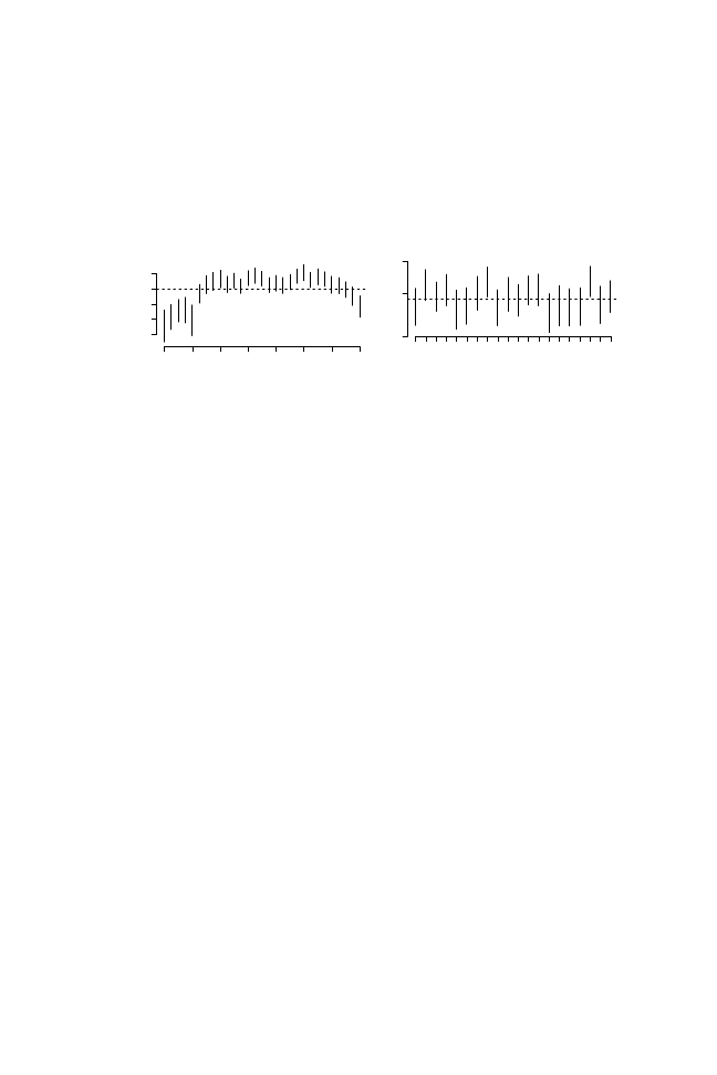
156

Curbing Bailouts

Figure 7.1: Posterior distribution of year- and country-speciﬁc intercepts

(median and 80% Bayesian credible intervals of the posterior distribution of

δ and α)

(a)

(b)

Year-speciﬁc random e

ﬀects (δ)

Country-speciﬁc random e

ﬀects (α)

1975

1979

1983

1987

1991

1995

1999

2003

−

Intercept

Year

●

Spain

Turkey

Egypt

Brazil

Bolivia

Peru

Thail

China

Ghana

Colomb

Kenya

Guate

Liberia

Uganda

Mozam

Laos

Indones

Guyana

Nicarag

Country intercept

●

control for transparency, which is assumed to be endogenous to political
regime and therefore a post-treatment variable in empirical analysis. Inclusion
of this confounding covariate in Models 2 through 4 does not change the
basic ﬁnding about the association between political regimes and probability
of failure or ﬁnancial distress, namely, that higher levels of democracy are
associated with lower levels of ﬁnancial distress.

Before commenting on the statistical and substantive importance of es-

timated regime e

ﬀects, I ponder brieﬂy on some other conclusions that are

supported by these models. Recall that I estimate country-speciﬁc and year-
speciﬁc random e

ﬀects in all models, though these are not reproduced in

Table 7.2 for the sake of space. Figure 7.1 (Plot a) displays year-speciﬁc ran-

dom e

ﬀects based on results from Model 4 (inferences about these parameters

remain essentially identical across models). As can be gleaned from this plot,
year e

ﬀects vary substantially throughout time, accounting for the fact that

the cross-country incidence of banking crises varied during the observation
period. In particular, the mid-1990s were years with more banking crises
than average, though the incidence of critical events declined relatively fast
in later years. The mid-to-late 1990s were, however, not an outlying period.

This distinction corresponds to the early years in the observation window,

i.e., the late 1970s, during which the number of crises around the world was
much lower. Note also that there exists variation in the propensity to fail
across countries that is not captured by included covariates. Figure 7.1 (Plot
b) displays summaries of the posterior distribution of a random sample of 20
country-speciﬁc intercepts. As can be seen from this plot, some countries are
slightly more prone to su

ﬀer banking crises during the observation period

than others, even after accounting for their regimes, economic makeup, and

Political Regimes and Banking Crises

157

ﬁnancial openness. In particular, Turkey, Thailand, and Indonesia appear as
countries with higher-than-average propensities to su

ﬀer banking crises. Out-

side of the countries included in this plot, other countries with random-e

ﬀect

intercepts that lie almost entirely above average are Malaysia, Mexico, and
South Korea. Though these are, incidentally, countries that at least during
some years throughout the observation period were non-democracies, their
political regimes do not fully account for their increased propensities to su

ﬀer

banking crises.

Despite the inclusion of year- and country-speciﬁc intercepts in all of

these models, several covariates at the data level show coe

ﬃcients that are

statistically di

ﬀerent from zero. This is the case of openness, growth, and

GDP per capita. Consistent with Table 7.1, relatively rich countries in the

sample are associated with higher levels of ﬁnancial distress. Recall that

“rich” countries in this sample are not advanced industrial democracies, as

most of these have been removed from the balanced sample, but middle-
income economies with the level of development of, say, Mexico. The lagged
value of GDP growth is a negative predictor of the probability of failure (i.e.,
higher rates of economic growth are associated with lower propensities to
su

ﬀer ﬁnancial distress a year later), and openness of a country’s capital

account is also negatively associated with the probability of failure. The
latter result holds after accounting for the time-varying incidence of banking
crises across countries. In contrast, Gini and transparency do not appear to be
relevant predictors of ﬁnancial distress. In Models 2 through 4, the posterior
distribution of the coe

ﬃcient on transparency is centered on the positive

orthant, but the spread of this parameter is simply too wide to be considered
as anything other than irrelevant. The same can be said of the coe

ﬃcient for

Gini in Model 3; though the point estimate is negative, consistent with the

argument in Chapter 3, the posterior distribution of this parameter is wide
enough to be practically centered on zero.

Compare now the inferences about the e

ﬀects of political regimes that

follow from di

ﬀerent models. Figure 7.2 provides a more intuitive sense of

the substantive importance of these regime e

ﬀects. Consider ﬁrst the posterior

predictive distributions of underlying ﬁnancial distress

∗

that obtain from

estimates in Model 2 (left plot) and Model 4 (right plot). The posterior
predictive distributions correspond to the values of the underlying ﬁnancial
distress score that we would expect to obtain at low (25

) and high (75

sample percentile) values of the Polity IV indicator while holding all other
covariates constant at mean sample values. Higher values of

∗

correspond

to higher latent ﬁnancial distress and therefore higher probability of su

ﬀering

a banking crisis. The spread of these distributions conveys a good deal of
uncertainty about the substantive importance of this e

ﬀect. As can be seen

from the left plot, the predictive distributions of

∗

under democratic and

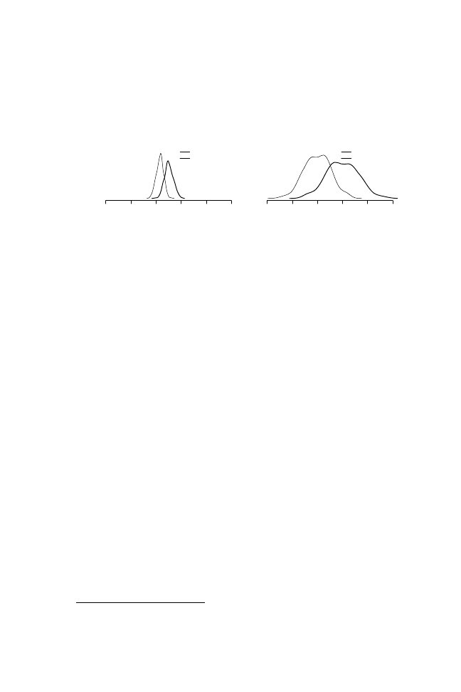
158

Curbing Bailouts

Figure 7.2: Posterior predictive distribution of ﬁnancial distress (

∗

) across

democratic and non-democratic regimes

Model 2

Model 4

−8

−6

−4

−2

Financial distress

Democracy
Non

−democracy

−8

−6

−4

−2

Financial distress

Democracy
Non

−democracy

non-democratic regimes are more or less distinct, but this e

ﬀect is muddled

when we consider the predictive distribution of

∗

based on the instrumental

variable estimates of Model 4. Even though the overlap in the predictive
distributions of

∗

corresponding to high and low values of democracy is

more extensive, we can still interpret these results as substantiating a positive
regime e

ﬀect.

Admittedly, the plots in Figure 7.1 do not include uncertainty derived

from estimation of other parameters in the model (random e

ﬀects, for ex-

ample). More importantly, though one can see substantial di

ﬀerences in the

distribution of ﬁnancial distress scores

∗

across regimes, it is di

ﬃcult to

build an intuitive understanding of the size of these di

ﬀerences, or to translate

them into relevant quantities, such as the probability of observing signiﬁcant
bank trouble and banking crises under alternative political regimes. Contrary
to predictions about ﬁnancial distress, which is a linear function of levels
of democracy, predictions about the frequency of systemic and borderline
banking crises depend as much on values of democracy scores as on the
values at which we hold other covariates constant. This follows from the
non-linear relation between probabilities

itk

and ﬁnancial distress scores

∗

(Equation 7.1).

To provide better intuition about the substantive e

ﬀects of political regimes,

consider Table 7.3, which displays the predicted frequency of borderline and
systemic crises based on draws from the posterior distribution of parameters
from Model 4. The counts in this table correspond to the number of times,
out of 100, that we would expect to see instances of borderline or systemic
events in an average country

/year.

To convey the level of uncertainty about

the e

ﬀect of regimes, this table also includes 80% credible intervals of the

The average year intercept corresponds to 2001, the average country intercept to Colombia’s.

Political Regimes and Banking Crises

159

predicted count of borderline and systemic crises. These predicted counts
are calculated at di

ﬀerent combinations of political regime and level of devel-

opment (in all cases

±1 SD from sample means), while holding constant all

other covariates at mean sample values.

Consider then the predicted frequency of di

ﬀerent types of events in an

average year. For example, based on the simulations of Table 7.3, I would
expect poor democracies to su

ﬀer between 2 and 8 years of systemic crisis

in a period of 100 years with probability 0.8. Among richer economies, the
incidence of borderline crises in the simulation is already a bit higher among
authoritarian than democratic regimes (5 vs. 3), but the e

ﬀect of democratic

regimes appears in full force when considering systemic crises: whereas “rich”
democratic regimes are expected to su

ﬀer between 6 and 13 crisis years in a

century, “rich” authoritarian regimes can expect to su

ﬀer between 21 and 33.

These relatively high counts obtain from more pronounced di

ﬀerences in the

probability of observing systemic banking crises on an average year, which I
estimate as 0.29 for authoritarian regimes and 0.09 for democracies. At these
rates, richer authoritarian regimes can expect to go about three and a half
years without a banking crisis, whereas richer democracies would be expected
to see a crisis every eleven years. This calculus is however premised on the
assumption that banking crises always last one year, when in fact the typical
length of systemic bank crises in the sample is about 2 to 3 years. As can be
gathered from this exercise, di

ﬀerences in the incidence of ﬁnancial distress

across political regimes are far from trivial even after factoring uncertainty
about regime e

ﬀects into the analysis. The analysis conﬁrms that democracies

are less likely to su

ﬀer high levels of ﬁnancial distress or, alternatively, that

they enjoy much lower probabilities of systemic failure. This result is in line

with a “strong” interpretation of political regime e

ﬀects.

Lest it be thought that the regime e

ﬀect is an artifact of the “modern-

ization syndrome” alluded to at the beginning of this section, recall that
these results are based on a balanced sample, and therefore less likely to
be model-dependent than an alternative analysis based on an unbalanced
sample of all available observations. In other words, the impact of democracy
uncovered in this analysis is not based on a sample of rich democracies on
the one hand, and poor autocracies on the other, but on a sample that includes
relatively rich and relatively poor democracies alongside relatively rich and
relatively poor authoritarian regimes. Furthermore, the estimates I present
correspond to an instrumental variables speciﬁcation that seeks to isolate
the truly exogenous component of variation in the political regime variable.

Recall the caveat about “poor” and “rich” countries; a country like Bolivia in this case would

be 1 SD below the average per capita GDP in the sample, and therefore epitomizes a “poor”
country, while a country like Mexico would be considered “rich” at about 1 SD above the sample
average.

160

Curbing Bailouts

Table 7.3: Predicted frequency of borderline and systemic crises under alter-

native political regimes and levels of economic development (point estimate
is the median of the posterior predictive distribution, interval estimate is the
80% credible interval)

Autocracies

Democracies

Rich

Poor

Rich

Poor

Borderline

(2–8)

(2–7)

(1–5)

(0–4)

Systemic

(21–33)

(13–23)

(6–13)

(2–8)

Though these e

ﬀects are not estimated in a design with random assignment

of countries to treatment and control, the model speciﬁcations inspected here
seek to reasonably approximate these conditions based on observational data.

7.2 Accounting Ratios as Indicators of Financial Distress

Expert scores constitute the most common way to measure incidence of
banking crises, and therefore underlying ﬁnancial distress. Be this as it may,
these indicators are not without ﬂaw. One problem with expert scores follows
from their binary nature, which makes it di

ﬃcult to use them to convey

relative magnitudes. In fact, in the comparison of Argentina and Mexico in
Section 7.1, part of the reason why Mexico obtains higher levels of ﬁnancial
distress than Argentina may be the fact that banking crises have tended to
last longer in Mexico, i.e., runs of consecutive 1’s in the Caprio et al. (2005)
database are longer in that country than in Argentina. To see how this might
a

ﬀect the conclusions of the previous section, consider the latent ﬁnancial

distress score Y

∗

: This value will tend to increase when Y

is coded 1 and to

decrease when it is coded 0. If a banking crisis lasts one year, Y

∗

will tend

to increase for one period to capture this information; however, if a banking
crisis lasts several years, Y

∗

will keep increasing to account for the string

of consecutive years within a country coded as 1. Countries with longer
banking crises (i.e., with longer runs of 1’s) will then appear to be countries

with harsher ﬁnancial distress. Harsher ﬁnancial distress may indeed lead to

longer banking crises, in which case inferences about the preventive e

ﬀects

of political regimes will remain unchanged. But what if this relationship does
not hold?

Political Regimes and Banking Crises

161

Table 7.4: Aggregate balance of a nation’s banking system (IFS series number

in parentheses)

Assets

Liabilities

Claims on other actors (22A-G)

Demand deposits (24)

Reserves (20-D)

Time deposits (25)

Foreign assets (21)

Other deposits (26A-G)

Capital (27)

Complicating this issue, the dichotomous coding of intrinsically continu-

ous variables magniﬁes measurement error, particularly in cases that are close
to a coding cutpoint. For example, a banking system that reduces its ratio
of non-performing loans from 11% to 9% in two consecutive years is hardly
out of the woods, but receives scores of 1 and 0, respectively, because these
values are on either side of the 10% cutpoint used by experts to decide that a
country’s banks are in critical condition. This is a drawback of any attempt to
aggregate intrinsically continuous data into discrete indicators. In the case of
banking crises, the problem is compounded by the fact that information about
underlying continuous indicators is not always very precise. For example,
there are at times important di

ﬀerences in the tally of ﬁscal costs of banking

crises that are derived from the inability to put a market value on the size of
losses. By the same token, it is di

ﬃcult to gauge relative improvement or

worsening in a banking sector that experts have tagged as being in critical

condition. A case in point is that of Mexico’s banking system in the 1980s.
Insolvent private banks were taken over by the government in 1982, slowly
nursed back to solvency, and reprivatized in the early 1990s, but there is
no way of assessing how healthy the banking sector progressively became
throughout the 1980s by relying exclusively on a dichotomous score.

For these reasons, it is worth looking at alternative indicators of ﬁnancial

distress. In this section, I use one such indicator built for this purpose from
information in the International Monetary Fund’s IFS. The IFS publishes
information on several categories of bank assets and liabilities aggregated
at the bank-system level. Though the indices are published on a quarterly
basis, I aggregate them annually to correspond with the frequency at which
independent variables are observed. Table 7.4 provides details about the
relevant IFS series used to construct the accounting indicators, and suggests
how these series correspond to di

ﬀerent elements of, as it were, the balance

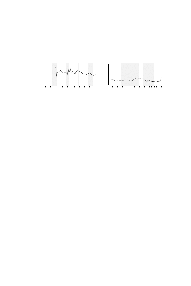
162

Curbing Bailouts

Figure 7.3: Net worth series for Argentina and Mexico (Capital

/Assets).

Series are built from the IMF-IFS and are laid over banking crises (gray bars)
identiﬁed by Caprio et al. (2005).

1975

1980

1985

1990

1995

2000

2005

Book

−

value net worth

Argentina

1975

1980

1985

1990

1995

2000

2005

Book

−

value net worth

Mexico

sheet of a country’s entire banking sector (see Chapter 2). Keep in mind that
by the rules of double-entry bookkeeping, assets should be equal to the sum
of liabilities plus capital.

From the series in Table 7.4, I consider the ratio Capital

/Assets as a

system-wide measure of ﬁnancial activity and refer to it as net worth. This
index has some resemblance to, but is not identical to, the regulatory capital-
asset ratio that one would ideally use to gauge bank insolvency. In fact, the

“capital” series in the IFS does not correspond to shareholders’ capital, but

is simply a measure of the book value of all assets in the national ﬁnancial
system compared to the book value of all liabilities. Because the IFS reports
these series at current values based on local currency units, the only way
to insure comparability across time and space is to consider this measure
as a proportion of total assets. The resulting ratio can be interpreted as
measuring the book-value net worth of a banking system. The index can
take negative values—corresponding to situations in which the book value of
liabilities outstrips the book value of assets and the banking system therefore
has negative net worth—though this kind of ﬂagrant insolvency is infrequent
in the data.

To familiarize the reader with this series, Figure 7.3 displays the time-path

of net worth in Argentina and Mexico, along with periods of systemic banking
crisis as recognized by experts. For reasons noted above, the correlation
between dichotomous scores and continuous indicators will be far from
perfect. However, as can be gleaned from this plot, it is possible to ﬁnd

The banking sector in the IMF-IFS series includes deposit-taking banks and savings and

loans, but not other ﬁnancial intermediaries like insurance companies or mutual funds admin-
istrators. The approach I take here is based on Ishihara (2005), who uses a similar method to
identify the occurrence of di

ﬀerent types of ﬁnancial crises.

Political Regimes and Banking Crises

163

Table 7.5: Mean and standard deviation of net worth conditional on political

regime (dichotomous index) and level of development (countries with per
capita GDP above

/below sample mean). Observations are at the country/year

level and are multiplied by 100.

Autocracies

Democracies

Rich

Poor

Rich

Poor

Net worth

.42

.14

.36

.21

.24)

.58)

.16)

.03)

251

364

435

175

correspondence between periods of systemic banking crisis identiﬁed by
experts and movements of the net worth variable. Consider for example
the series for Argentina, which follows recognized periods of banking crisis
relatively closely, with dips in the series in 1988–1989, 1994–1995, and
at the beginning of 2002. In the case of Mexico, we can see a gradual
improvement in aggregate net worth in the late 1980s in the period preceding
bank privatization, and then a precipitous decline starting in 1994, with a
further drop in net worth around 1998–1999.

As I did previously, I try to build as strong as possible a case for a causal

interpretation of the political regime e

ﬀect. To do so, I draw again a sample

of countries that ensures su

ﬃcient covariate balance across types of political

regime (see Section 7.1.1). Because the sample of countries for which the
IFS provides information is not identical to the sample of countries included
in Caprio et al.’s tally of banking crises, the set of countries on which I base
the analysis in this section is smaller (N

= 51) and slightly diﬀerent from that

of Section 7.1.

I expect democratic regimes, on average, to be associated with higher val-

ues of net worth, which would correspond to lower levels of ﬁnancial distress.

Table 7.5 breaks down the distribution of net worth across political regimes

and across levels of economic development based on information from the

The net worth series are stationary for all countries, as conﬁrmed by KPSS stationarity tests

(Baum and Sperling 2001; Kwiatkowski, Phillips, Schmidt and Shin 1992).

See Appendix A.2.5. Coverage of the IFS series is uneven across countries. Lack of

information in some IMF-IFS series led to loss of data for India, Israel, Japan, Norway, Senegal,
Singapore, and United Kingdom. These countries were not considered in the matching procedure.
For other countries, data exist at quarterly frequency from 1975 to date, but there are some
gaps in the series. Missing values of the dependent variable are assumed missing at random
and updated through the estimation process (84 values are missing among 1,173 country

/year

observations).

164

Curbing Bailouts

balanced sample. As in Table 7.1, Table 7.5 uses categories corresponding
to above and below mean income for level of development and the regime
indicator of Przeworski et al. (2000) for democratic and non-democratic
regimes. The cross-tabulation does not support my expectations, as the cate-
gory with highest average net worth is that of poorer non-democratic regimes.
Furthermore, average net worth across all democracies, regardless of level
of development, is 10.6 (SD

= 5.4), as opposed to 11.5 (SD = 7.4) across

non-democracies; though substantively small, this di

ﬀerence is statistically

signiﬁcant at the 95% conﬁdence level. A skeptical reader of these data would
remark on the fact that banks do not always face incentives to report their
real ﬁnancial status to domestic authorities, and that these incentives are less
powerful precisely in poorer non-democratic countries. If this interpretation

were indeed accurate, we would expect the regime coe

ﬃcient to be biased

against the hypothesis that I purport to verify—a far less complicated situa-
tion than the alternative, since any results that obtain in the expected direction
can only be presumed to be larger in the absence of measurement error. In
any case, recall that the matching process that I employ to obtain a more
balanced sample of observations does not take into consideration the values
of the dependent variable of interest, so sample choice was in no way guided
by the distribution of net worth across regimes.

To build a reasonable model within which to estimate regime e

ﬀects,

one must make several assumptions about the process that drives net worth.
More fundamentally, building a model of the association between political
regimes and net worth in a context of time-serial cross-sectional data requires
appropriate assumptions about underlying dynamics. Consider then a model

where net worth in country i at time t is drawn from a normal distribution—

i.e., net worth

∼ N(μ

, σ

2
i

)—where

has an autoregressive distributed lag

(ADL) structure, as in Equation 7.5:

= α

+ β

Net worth

−1

+ β

Regime

+ β

Regime

−1

(

itk

+ γ

−1k

)

(7.5)

As DeBoef and Keele (2008) point out, this model is identical to an error

correction model but relies on a di

ﬀerent, more intuitive, parameterization.

The ADL model is particularly useful when theory provides little guidance

about the lags at which independent variables a

ﬀect the dependent variable.

In this case, the hypothesis of interest is that the e

ﬀect of political regime on

net worth is positive, but it is not clear from the theory in Chapter 3 whether

we should expect this e

ﬀect to be spent out contemporaneously (which would

be captured by

) or whether regime continues to a

ﬀect net worth after a

1-period lag (captured by

). Furthermore, we can calculate a “dynamic

Political Regimes and Banking Crises

165

multiplier” e

ﬀect from this model, i.e., an estimate of the long run or total

ﬀect of regime on net worth distributed over future time periods.

The

value of net worth for country i at year t is also a function of other covariates
measured at the country-year level (X

), whose e

ﬀects are also partitioned

into contemporaneous (

) and lagged (

) e

ﬀects. I rely on the same battery

of covariates as in the previous exercise: capital openness, GDP growth, and
per capita GDP. I also estimate random country intercepts

because banking

systems di

ﬀer systematically in their average levels of net worth throughout

the period under study, likely a consequence of unobserved covariates—like
regulatory regimes or central bank status. Note also that I consider the
possibility of heteroscedasticity, i.e., that the variance of net worth scores may
be di

ﬀerent across countries. By estimating country-speciﬁc variances σ

2
i

, I

admit the possibility that countries may have di

ﬀerent patterns of year-to-year

book value net worth.

7.2.1 Results

Table 7.6 reproduces coe

ﬃcient estimates from various speciﬁcations of the

basic model described in Equation 7.5. To convey the main results of the
analysis, I discuss ﬁrst the simplest speciﬁcation (Model 1). This model
includes random country-level intercepts and country-speciﬁc variance pa-
rameters (not shown for the sake of space). In this speciﬁcation, the strongest
positive predictor of system-wide net worth is a country’s lagged level of
development, captured by per capita GDP (log scale). Values of average
economic growth are, contrary to expectations, negatively correlated with net
worth, whereas openness, which captures the degree to which capital is able
to ﬂow across country borders, has a contemporaneous positive short term
association with the dependent variable in line with results in Section 7.1.

Across the di

ﬀerent speciﬁcations, there are no relevant changes in estimates

of the coe

ﬃcients for the main control variables.

I o

ﬀer several models based alternatively on Przeworski et al.’s dichoto-

mous regime indicator (Models 1 and 3) and the continuous Polity IV indicator
of democracy (Models 2 and 4); both indicators are coded so that higher val-

Based on the notation of Equation 7.5, the dynamic multiplier is k

= (β

+ β

)

/(1 − β

WinBugs code appears in Appendix A.3.6. To complete the description of the model,

I stipulated di

ﬀuse prior distributions on parameters: β, γ ∼ N(0, 0.01), α ∼ N(0, 0.001),

σ ∼ Uniform(0, 100). The dependent variable is rescaled by a factor of 100 and independent
variables are standardized to aid convergence. Descriptions of the posterior distribution of
parameters are based on 500 to 1,000 draws from two separate chains, thinned every 10

iteration, after apparent convergence. Convergence was swift and clean and was monitored using
the Gelman-Rubin

R statistic.

To be precise, higher degrees of openness are associated with lower probabilities of banking

crises (Table 7.2) and higher values of net worth (Table 7.6).

Table 7.6: Autoregressive distributive lag models of aggregate net worth.

Point estimates are the median of parameter posterior densities (standard
deviation of parameter posterior densities in parentheses). Statistic k is the
dynamic multiplier e

ﬀect of regime.

Model 1

Model 2

Model 3

Model 4

Indicators

REG

Polity IV

REG

Polity IV

Country

/year level

Net worth

−1

.823

.822

.878

.881

.018)

.019)

.016)

Regime

.084

.135

.085

.153

.116)

.155)

.112)

.160)

Openness

.173

.250

.158

.243

.121)

.135)

.128)

.126)

Growth

−0.123

−0.129

−0.122

−0.123

.093)

.097)

.091)

.093)

GDP pc

.043

.140

−0.376

−0.486

.434)

.019)

.449)

.459)

Regime

−1

.225

.189

.174

.092

.117)

.157)

.115)

.167)

Openness

−1

−0.097

−0.151

−0.103

−0.170

.120)

.138)

.127)

.139)

Growth

−1

−0.024

−0.018

−0.001

.027

.088)

.090)

.086)

.091)

GDP pc

−1

.729

.628

.391

.485

.430)

.461)

.456)

.451)

Country level
Intercept

.489

.462

.235)

.248)

Inequality

.070

.012

.227)

.237)

Transparency

−0.121

−0.184

.322)

.327)

.753

.819

.131

.054

.371)

.442)

.513)

1,122

Countries

DIC

5,096

5,102

5,078

5,084

108

111

Political Regimes and Banking Crises

167

ues correspond to democratic regimes. Across these di

ﬀerent speciﬁcations,

the coe

ﬃcients of main concern are those that correspond to immediate (t)

and lagged (t

− 1) eﬀects of regime on net worth. In Model 1, for example, the

contemporaneous e

ﬀect is positive, but straddles 0 (0.084 ± 0.12), whereas

the posterior distribution of the lag e

ﬀect has most probability mass to the

left of 0 (0

.225 ± 117). These two parameters capture the short-term eﬀect of

political regime on a banking system’s book-value net worth. Aside from this
immediate e

ﬀect, the dynamic multiplier k statistic at the bottom of the table

reveals the long-run e

ﬀect of regime on net worth.

Across all four speciﬁcations, the short- and long-run e

ﬀects of political

regime are consistently positive, though there are admittedly noteworthy
variations in the estimated size of these e

ﬀects and in the degree of uncertainty

that surrounds them, especially in the short run. The dynamic multiplier
statistic suggests that average net worth over the long run can be several points
higher in democratic than in non-democratic regimes. For example, based
on coe

ﬃcients for Model 1, the long-run diﬀerence in net worth between

democratic and non-democratic regimes is 3

.57 (±0.76) points, which is not

a trivial amount considering that the standard deviation of the unconditional
distribution of net worth is 6.48. Similar estimates of the long-run positive
impact of democracy on net worth follow from the rest of the models.

These long-run e

ﬀects are the result of slow accumulation, as in the short

run the estimated e

ﬀects of regime are more uncertain and much smaller in

terms of substantive magnitude. In particular, Models 3 and 4 reveal a smaller
regime coe

ﬃcient; these models include average inequality and transparency

measures at the country level and provide a slightly better ﬁt based on the
deviance information criterion reported in the last row of Table 7.6.

Since

they provide the most conservative estimates of the regime coe

ﬃcient, I focus

on Models 3 and 4 to gauge the substantive importance of this variable as
a predictor of net worth in the short run, that is, considering the regime
variable ﬁxed during two consecutive years. For this purpose, the left panel in
Figure 7.5 plots the posterior predictive distribution of net worth for the two
values of the political regime dichotomous indicator while holding all other
variables at their mean sample values. As can be gleaned from this graph,
the posterior predictive distributions of net worth under these two regimes
overlap. In fact, they overlap to such an extent that there is a non-negligible
probability (

≈ 0.14) that non-democratic regimes may have higher net worth

in the short run. In substantive terms, the average regime e

ﬀect based on

Country averages of inequality and transparency are based on available information for each

country. They are added as predictors of country intercepts, i.e.,

= δ

+ δ

Transparency

Inequality. The coe

ﬃcient of inequality is basically centered on 0; the posterior distribution of

the coe

ﬃcient of transparency has most probability mass to the left of 0, but also straddles this

value.

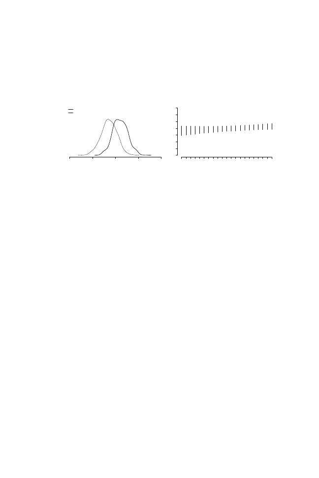
168

Curbing Bailouts

Figure 7.4: Posterior predictive distribution of net worth across democratic
and non-democratic regimes (a) and partial regression of country-speciﬁc net
worth variance on average regime scores (b)

(a)

(b)

Net worth

D
A

−10

−8

−6

−4

−2

9 10

Net worth

Polity IV

●

the scenario of the left plot of Figure 7.5 can be summarized as follows:

Within two years, the banking system’s book-value net worth of an average

authoritarian country would lie between 10.28 and 11.15, and between 10.82
and 11.62 under an average democratic regime (80% credible intervals).

The right panel of Figure 7.5 displays a similar exercise corresponding

to Model 4, which is based on the continuous Polity IV score as the relevant
indicator of democracy. In this graph, point estimates correspond to the
median of the posterior predictive distribution of net worth. In Model 4, the
contemporaneous regime e

ﬀect is 0.15 (±0.16) and the lagged eﬀect is 0.09

(

±0.17); the posterior distributions of these eﬀects are centered on positive

values, but wide enough to straddle 0. Consequently, the plot suggests a barely
noticeable upward trend in the posterior predictive distribution of net worth;
at the left end of the scale, an average country with the least-democratic Polity
IV score of –10 would be expected to have net worth between 9.90 and 11.34,
whereas an average country with the most-democratic Polity IV score of 10
would have a net worth range between 10.81 and 11.72 (again, these are 80%
credible intervals). The positive, albeit small, short-run e

ﬀects of regime in

these models are still consistent with long-run dynamic multipliers of 2

.13

(

±0.52) and 2.05 (±0.51), respectively.

Aside from understanding regime e

ﬀects on net worth levels on a short-

and long-run basis, these models o

ﬀer a glimpse into potential association

between political regime and overall net worth stability. To do so, we can
analyze cross-country patterns of variability of the net worth series. Recall
that the models reported in Table 7.6 include unmodeled country-speciﬁc
intercepts (

) and variance (

2
i

) parameters. The ﬁrst set of parameters

captures the average level of net worth in each country throughout the obser-

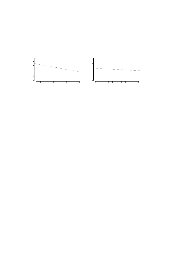
Political Regimes and Banking Crises

169

Figure 7.5: Partial regressions of country-speciﬁc net worth intercept (

α)

and variance (

σ) parameters on average regime scores and average GDP per

capita, based on Model 4 in Table 7.6

(a)

(b)

−10

−6 −4 −2

.01

.02

.03

Average democracy score, 1981

−2003

Country intercepts

●

●●

●

−10

−6 −4 −2

−

Average democracy score, 1981

−2003

Net worth variance

(log scale)

●

vation period, whereas variance parameters capture the amount of variability
around this average level. Figure 7.5 displays added-variable plots of point
estimates of country-speciﬁc intercepts (Plot a) and country-speciﬁc variance
parameters (Plot b) as a function of a country’s average level of democracy,
based on Model 4. As can be seen in Plot a, countries with higher average
levels of democracy throughout the observation period tend to have slightly
lower average net worth, as suggested by the category breakdown of Ta-
ble 7.5. Plot b reveals no systematic e

ﬀect of average levels of democracy

on country-speciﬁc variation in net worth. Though the association between
country-speciﬁc variances and average levels of democracy is negative, sug-
gesting that democratic regimes have more stable patterns of net worth, this
result is not statistically relevant.

7.3 Concluding Remarks

I have sought to understand in this chapter whether the e

ﬀects of democratic

regimes on banking policy extend beyond limiting government propensities
to implement bailout policies. This enterprise is complicated because the the-
oretical concepts that one would like to measure are intangible probabilities
of failure and solvency status of banking systems. I have resorted to banking
crises indicators and measures of the book-value net worth of banking sys-
tems as tangible indicators of these theoretical concepts. Furthermore, the
observational nature of the data limits our ability to make causal inferences

In contrast, I ﬁnd that “richer” countries (again, due to the use of a balanced sample these

tend to be middle-income economies) have conspicuously less volatile net worth series (results
not shown).

170

Curbing Bailouts

about parameters. As I did in Chapter 6, I built a case for causal interpretation
of model parameters. To do so, I have resorted to matching methods that
correct for covariate imbalance and techniques such as instrumental variables
that contribute to isolate truly exogenous variation in a crucial regressor to
comply with the assumption of ignorability of treatment assignment. Based
on these assumptions, I conclude that democratic regimes limit the possibility
of ﬁnancial distress and bolster the overall solvency status of banking systems,
though the true size of the e

ﬀect is diﬃcult to gauge. This ﬁnding is in line

with Propositions 2 and 3.

The analysis in this chapter rounds up the empirical evidence that I

marshal to substantiate an optimistic view of democratic accountability. The
evidence presented in this chapter is consistent with a view according to

which economic actors look forward and rationally anticipate government

policy output, incorporating these expectations into current behavior. In my
view, democracy reins in politicians and forces them to consider the welfare
of taxpayers when devising programs to redress banking crises. Bankers
and entrepreneurs understand the e

ﬀect of this constraint on government

action, and thus discount the probability of generous bailouts funded by
taxpayers. This knowledge a

ﬀects their economic decisions enough so that

the probability of bank failure and the book-value net worth of banking
systems are noticeably lower under democracies than under authoritarian
regimes.

Conclusion

The term “bailout” has an unmistakable pejorative connotation in banking

policy. This connotation builds up with every instance of government support
to failing banks, regardless of the extent of this support and its stated policy
objectives. Bank bailouts violate innate norms of fairness because they
suggest that governments protect powerful actors from their own greed and
folly at the expense of common citizens. And yet, banks are indeed special;
they are highly leveraged, intricately intertwined, and su

ﬀer to a larger extent

than non-ﬁnancial ﬁrms from mismatches in their asset

/liability structure. Not

only do these features subject the best-managed institutions to the possibility
of failure, but failure of even a small bank threatens ample ripple e

ﬀects that

may destroy trust in the basic solvency of a country’s ﬁnancial system.

We can understand government policies to contain banking crises within a

dual economic and political logic. The economic logic behind public support
builds on Bagehot’s doctrine, a rule that requires a lender of last resort to
provide liquidity to distressed banks. This kind of forceful intervention is
necessary to restore stability to a country’s ﬁnancial system and, if done right,
can strengthen the banking sector by pruning the weakest institutions. After
all, Bagehot’s doctrine also calls upon governments to force the orderly exit
of insolvent banks. When government interventions are limited to following
Bagehot’s precepts, it is hard to construe them as examples of robber baron
capitalism gone awry. The lender of last resort is meant to temporarily “ﬁll
in” for the market mechanism: it sorts banks out according to quality, lends
freely to solvent banks, and shuts insolvent banks down. Taxpayers do not
stand to lose because last resort loans are doled out at a penalty rate and on
good collateral.

Be this as it may, governments very often overstep the boundaries of

Bagehot’s doctrine and provide support to banks that hardly deserve it. Bage-
hot’s doctrine is often criticized because it is in practice di

ﬃcult for regulators

and politicians to perform the kind of triage on which it is premised. After
all, if information about the ﬁnancial status of banks is su

ﬃciently unclear

171

172

Curbing Bailouts

that it prevents markets from allocating liquidity to deserving banks, what
guarantees that government agencies will be any better at separating dis-
tressed but fundamentally solid institutions from those fated to the dustbin of
history? Under conditions of extreme asymmetric information, government
agencies are as helpless as other economic actors in reaching correct conclu-
sions about the true ﬁnancial status of banks. When one adds concerns about
systemic risk—i.e, about the possibility that insolvency of one or a handful of
banks will extend to other institutions—it is easier to see how even reluctant
governments will seem eager to extend a helping hand to banks.

This book has shown that there exists wide variation in the kind of policies

that governments put together to manage banking crises, and that an important
part of this variation can be traced back to di

ﬀerences in political regimes

across countries. Banking crises can only be avoided at very hefty cost, for
example by mandating extremely high rates of capitalization and forcing
banks to invest in safe and liquid assets. Needless to say, these options

would also eliminate a banking system’s ability to allocate credit to desirable

projects and would very likely slow down a country’s pace of economic
growth. Barring such extreme policies, it is foreseeable that banks will
continue to fail every now and then. Banks, like other actors in ﬁnancial
markets, are in business for the promise of future returns; these promises
cannot always be kept, even under the best intentions.

I have argued that the political logic that underlies bailouts may help

tame the more costly aspects of banking policy. I consider that democratic
regimes are better than authoritarian regimes at countering pressures from
organized groups that face concentrated losses in the event of a banking crisis.
Democracies achieve this e

ﬀect by subjecting governments to meaningful

periodic elections. Though electoral accountability might not always make
for a high-powered set of incentives pushing governments toward imple-
menting the policy preferences of unorganized voters, it certainly constrains
democratic governments enough to keep them away from the most blatant
and intrusive forms of bank bailout. In this regard, the evidence reviewed in
Chapters 5 and 6 conﬁrms that governments in democratic regimes have on
average lower bailout propensities than governments in authoritarian regimes.
By showing that the bailout policies put forth by democratic governments
tend to be less expansive, I engage a debate on the possibility and limits of
a “democratic advantage” in policy-making, a debate that has been pursued
in many ﬁelds of inquiry within political economy, for example in research
on foreign direct investment (Jensen 2006), sovereign debt (Saiegh 2005;
Schultz and Weingast 2003), credit risk assessments (Archer, Biglaiser and
DeRouen 2007; Vaaler and McNamara 2004), and monetary policy (Desai,
Olofsgård and Yousef 2003). My contention that democratic regimes tend to
enact less intrusive bailouts than non-democracies should not be construed

Conclusion

173

as a full endorsement of democratic policy-making. To do so, one would
need to show that banking policy output under democratic regimes is optimal
according to some uncontroversial yardstick. Given the amount of uncertainty
that surrounds policy choice during banking crises, ﬁnding such an uncon-
troversial yardstick is di

ﬃcult at best. Building that yardstick would require

answers to the following questions: Is the decision to pass some ﬁnancial
losses on to taxpayers the optimal way to safeguard the banking system? If
so, what is the minimum amount of ﬁnancial losses that must be socialized
in order to guarantee the stability of a country’s banking system? Thus, an
important limitation of my research is that is not meant to answer questions
about the optimality of democratic policy-making in the midst of banking
crises. In other words, though I can say with a high degree of conﬁdence
that democratic regimes are less prone than non-democratic regimes to im-
plement policies that socialize ﬁnancial losses, I cannot say how close or
far away democratic regimes are from solving banking crises in an optimal
manner. In the face of current ﬁnancial distress in the banking systems of core
democratic economies, it would be extremely important to understand the
institutional conditions under which electoral accountability has the largest
impact on limiting government intervention to the bare minimum. This of
course implies a nuanced understanding of banking policy among countries
that have enjoyed stable democratic governance in the recent past.

My analysis also supports the view that the salutary e

ﬀects of electoral ac-

countability extend beyond simply limiting the propensity of governments to
bail out troubled banks. The theoretical argument is premised on the recogni-
tion that rational actors are capable of anticipating government policy choices.
If bankers, entrepreneurs, and even bank creditors and debtors anticipate that
bailouts will not be forthcoming in case of ﬁnancial distress, this realization
ought to change their economic behavior. A direct test of this argument

would require inspection of the risk-taking behavior of entrepreneurs and

bankers under di

ﬀerent political regimes. Given the diﬃculty of carrying

out such a test in a large number of countries, I chose to corroborate testable
implications of this argument. First, I inspected the frequency of banking
meltdowns under alternative regimes. I found that democratic regimes tend
to su

ﬀer lower counts of banking crises than authoritarian regimes. Second, I

inspected the level of association between political regimes and accounting
ratios that more directly reﬂect the book-value net worth of banking systems.
In this case, I also found that democratic regimes have a positive e

ﬀect on the

aggregate net worth of banking systems, especially in the long run. Again, I
do not mean to dress up this conclusion as support for the proposition that
democratic accountability su

ﬃces to prevent banking crises; it clearly does

not, as is obvious from the fact that the subprime-mortgage crisis started in
the core democratic nations of the global ﬁnancial system.

174

Curbing Bailouts

These ﬁndings are premised on a number of assumptions about the inner

workings of politics and ﬁnancial intermediaries and about the characteristics

of observed samples. I have strived to make explicit all the assumptions
that underlie the empirical sections of the book. My conclusions about the
salutary e

ﬀects of democratic regimes on banking policy ultimately stand

on analysis of observational data. Under ideal circumstances, one would be
able to randomly assign treatment (in this case, democratic accountability)
to di

ﬀerent polities, thus complying with necessary conditions required to

estimate causal e

ﬀects (Holland 1986; Rubin 1974). When random treatment

assignment is not possible, as is common in many ﬁelds of scientiﬁc research,
estimates of causal e

ﬀects are only as good as the eﬀort spent in approaching

these necessary conditions. E

ﬀort must be spent in controlling for relevant

covariates, obtaining balanced samples, and above all approximating the
assumption of exogenous independent variables that underlies causal analysis.
In the analysis of observational data, careful statistical modeling is still the
best way to approximate a causal interpretation of e

ﬀect parameters. I believe

that my analysis complies with the extant conditions required to provide
such an interpretation of regime e

ﬀects; ultimately, the results stand on the

verisimilitude of these assumptions, which explains my insistence in vetting
them thoroughly.

I have also laid out clearly all theoretical assumptions about the interac-

tion between governments, entrepreneurs, and bankers. I have been careful to
select these assumptions so that they correspond with accumulated knowledge
about politics and policy choice. Some of these assumptions, like the as-
sumption of rational choice and expected utility maximization, are ubiquitous
and more or less consensual in applied work in political economy. Wherever
necessary, I provide theoretical justiﬁcation for all the other assumptions that
underlie the main argument—assumptions about order of play, agent payo

ﬀs,

and exogenous parameters. There are, however, a number of assumptions that
have remained implicit in my analysis. In my view, future work should aim
to revisit and perhaps relax these assumptions.

First, I have not considered certain institutional aspects of banking reg-

ulation in great detail. I have given short consideration to issues such as
autonomy of bank regulators, transparency in bank accounting standards, and
distribution of supervisory and regulatory functions among more than one
agency. In particular, autonomy of bank regulators stands out as a factor that
may a

ﬀect the bailout propensity of governments. Satyanath, for example,

considers that the ability of developed democracies to get away with liberal
capital controls without succumbing to major banking crises may result from
independence of regulators from political pressures (Satyanath 2006). Indeed,
if bank regulators have a preference for stringent regulation and if they are
indeed autonomous from politicians, it certainly follows that they will be

Conclusion

175

successful in preventing banking crises.

There are however reasons to suspect that this explanation is incomplete.

To begin with, governments undergoing banking crises have great incentives

to revamp their banking agencies and regulatory structures, so these institu-
tions are more aptly seen as endogenous to the political process. Furthermore,
even autonomous regulators may have an incentive to engage in forbearance.

After all, the objective of a competent autonomous regulator is to ensure that

banks are solvent by monitoring them continuously and preventing ﬁnancial
distress. Bank closures, even if justiﬁable, are an unequivocal signal that
the bureaucrat failed in her mission to prevent insolvency. Finally, even
if one argues that “better” regulatory agencies have a beneﬁcial impact on
banking policy, one should provide an answer to the question of where the
political impetus or willingness to supply appropriate regulatory frameworks
comes from. In my opinion, the decision to supply better regulation is mostly
determined by links of political accountability. It may well be that mature
democracies have an advantage in counting with independent regulators, but
that is only because they have had ample time to learn that such institutional
settings make for better banking outcomes. Many young democracies may
simply have failed to discover the beneﬁts of such regulatory structures. Once
they undergo a ﬁnancial crisis, and therefore understand how devastating
these events can be, the incentives to adopt these institutions may very well
increase. Such incentives seem to be at work even in older democracies, like
the United States, where the subprime-mortgage crisis of 2007 and 2008
has brought about urgent calls to regulate ﬁnancial products that have been
largely out of the purview of banking agencies in the past. At the end of the
day, the best regulatory schemes cannot dissipate entirely the temptation of
economic actors to increase risk-taking if these actors can count on shifting
part of the downside risk to society at large. In this regard, non-democratic
regimes provide economic actors with reasons to anticipate larger degrees of
socialization of bank losses.

A second implicit assumption concerns the close identiﬁcation I make

between banks and banking systems, i.e., between the components of a
system and the system as a whole. My theoretical argument considers the
interaction between a set of entrepreneurs and a decision-maker, with a single
bank that plays the passive role of gathering deposits and lending them to
entrepreneurs in exchange for interest payment. I have then considered this
single bank as an example of how governments react vis-`a-vis the whole
banking system. In short, I have obviated consideration of the problem of
aggregation. The “single bank” assumption, I believe, has been extremely
productive in generating testable implications, and is in fact defensible if one
considers this bank to be a representative agent. However, even a cursory
reading of Chapter 4 suggests that banking systems cannot always be reduced

176

Curbing Bailouts

to the sum of their component units. For starters, banks come in di

ﬀerent

sizes and attitudes towards risk, and belong in di

ﬀerent categories that may

receive unequal policy treatment. More importantly, banking crises usher
in periods of consolidation in which larger banks are often called upon

(and subsidized) to take on smaller banks. Under these circumstances, it is
worthwhile to consider whether the very structure of a country’s banking

sector may have an impact both in producing widespread insolvency and in
fostering certain types of crisis-management policies. On the one hand, what

we know about the logic of collective action suggests that more concentrated

banking sectors may be better able to push for bailouts in case of ﬁnancial
distress.

On the other hand, an oligopolistic organization of banking systems

might diminish incentives for cutthroat competition in the banking industry
and might produce more cooperative outcomes in times of distress.

A third implicit assumption has to do with the consideration of national

banking as a closed system. This assumption has two consequences. First, of
course, the possibility of ﬁnancial contagion has been discussed extensively
in the literature and remains an active area of research. I have not explicitly
considered channels of ﬁnancial contagion across countries, but I made an ef-
fort to allow the possibility of variable correlations across countries within the
same time-period. I am more interested about a second potential consequence
of this implicit assumption. I have analyzed national banking systems as if
these operated within self-contained polities, an assumption that becomes less
accurate as banks, particularly those based in developed economies, continue
to increase their reach beyond national borders. This phenomenon is not
new, but the pace at which international banks take up market share in the
retail banking sector of many economies is staggering. At the same time,
bank regulation and supervision is failing to keep up with the pace of this
process. Admittedly, international e

ﬀorts enshrined in the Basel Accords have

helped standardize “best practice” banking regulation around the world; these
e

ﬀorts have been interpreted as the fruit of coordination among sovereign

states to prevent negative externalities from a banking crisis in one country
from spilling over to other countries (Kapstein 1994). However, the crux of
the problem is that as large banks deepen their commitment to act globally,
banking regulation continues to be essentially a national endeavor. In fact, an
alternative interpretation of the Basel Accords suggests that US regulators
pushed for it in an e

ﬀort to drag down the competitiveness of foreign banks

gaining market share on American banks (Oatley and Nabors 1998; Singer
2007). In this interpretation, far from helping authorities keep up with the
global reach of banks by endowing an international authority with regulatory

Be this as it may, an indicator of bank concentration fails as a predictor of bailout propensities

(Rosas 2006).

Conclusion

177

capacity, these e

ﬀorts at international coordination may simply increase the

occurrence and severity of banking crises. It is thus important to expand our
understanding of the conditions under which national governments, regard-
less of their political regime, can coordinate e

ﬀectively to deal with banking

crises.

Appendices

A.1 Mathematical Proofs for Chapter 3

erivation of Equation 3.1. Set the Lagrangean equation

= π(R(π) − 1 − r) − (1 − π)w + λ(R(π) − 1 − r).

I disregard the possibility that the constraint is binding, i.e., R(

π) − 1 = r,

as there is no reason to assume that an entrepreneur would be content with
risking capital in exchange for a return that barely covers interest payments
in the good state. Therefore, the ﬁrst-order necessary condition requires com-
pliance with the following conditions:

∂L/∂π = 0, λ = 0, and R(π) − 1 > r.

Satisfying the ﬁrst-order condition implies that

E(U

)

= 0, which obtains

when R(

∗

)

+π

∗

(

∗

)

= 1−r −w. To show that π

∗

is an interior solution, con-

sider

π = 0 and π = 1 as candidate solutions. In the ﬁrst case, the ﬁrst-order

condition would be rewritten as R(0)

= 1 + r − w, but this equality cannot

hold because R(0)

> 1 and 1 + r − w < 1. In the second case, the ﬁrst-order

condition would be R(1)

+ R

(1)

= 1 + r − w. By assumption, R(1) = 1 and

(1)

≤ −1, so R(1) + R

(1)

≤ 0, while 1 + r − w > 0. This shows that the

endpoints 0 and 1 cannot be solutions. To show that equilibrium choice

∗

a maximum, note that the second-order condition is 2R

(

∗

)

+ π

∗

(

∗

)

< 0,

which holds because R

< 0 and R

< 0 by assumption (see fn. 4).

robabilities of different endstates conditional on signals. Using Bayes’

rule, the probabilities for the di

ﬀerent endstates of the game upon observing

signal s

∈ {s

, s

} are

Pr(R

)

Pr(R

) Pr(s

)

Pr(s

)

∗

= 1

Pr(R

)

Pr(R

) Pr(s

)

Pr(s

)

− π

∗

)

· 0

∗

= 0

178

Appendices

179

Pr(R

)

Pr(R

) Pr(s

)

Pr(s

)

∗

− q)

∗

− q) + (1 − π

∗

)

Pr(R

)

Pr(R

) Pr(s

)

Pr(s

)

− π

∗

)

∗

− q) + (1 − π

∗

)

roof that ∂c

∗

/∂σ > 0. The formal proof that democratic governments are

less likely to engage in forbearance in less egalitarian societies follows from
signing the partial derivative of c

∗

with respect to

σ, which parameterizes

inequality, as positive. Applying the chain rule, the relevant derivative is

∂c

∗

∂σ

∂c

∗

∂¯y/y

∂σ

(A.1)

Writing a

= π

∗

r and b

= (1 − π

∗

)(1

− q)(1 − w), the ﬁrst term in Equation A.1

∂c

∗

∂¯y/y

− a)b

+ b(¯y/y

− 1))

which is negative if a

> b. This will be the case if π

∗

> (1 − π

∗

)(1

− q)(1 − w),

that is if

∗

> (1 − q)(1 − w)/(r + (1 − q)(1 − w)), which is guaranteed to

hold. To see this, assume that

π ≤ (1 − q)(1 − w)/(r + (1 − q)(1 − w)); this

implies that c

≤ 0, which in turn means that F(c

)

= 0, which ﬁnally leads

to 0 expected utility for the entrepreneur. But the entrepreneur can guarantee
herself a positive payo

ﬀ by choosing π > (1 − q)(1 − w)/(r + (1 − q)(1 − w)).

Thus, the numerator is negative, the denominator positive, and the entire

expression negative.

From the deﬁnition of the Pareto distribution, write ¯y

(

σ −

1)2

/σ

−1

. The second term in Equation A.1 is

∂¯y/y

∂σ

(

σ − 1)

−1/σ

+ 2

−1/σ

log(2)

−1

− 2

−1/σ

(

σ − 1)

σ(log(2) − 1) − log(2)

σ(σ − 1)

/σ

Since

σ > 1, the denominator of this expression is positive. The numerator,

however, is negative because log(2)

> σ(log(2) − 1). To see this, rearrange

terms and rewrite this latter expression as 1

log(2)

> σ, which always holds

because log(2)

< 1. Consequently, the partial derivative of c

∗

with respect to

σ is positive, which implies that as inequality decreases (i.e., σ increases),
democratic governments have more incentives to forbear.

180

Appendices

roof of Condition 3.9. The entrepreneur’s problem is to set

∗

≡ argmax

)

The ﬁrst order condition obtains when

∂E

)

∂κ

= π

∗

(

κ) − (1 − π

∗

)

αw¯y = 0,

which readily yields Condition 3.9. There cannot be a corner solution at

∗

= 0, because this would imply Z

(0)

−π

∗

αw¯y and this violates the

assumption that Z

(0)

= ∞ (see fn. 22). However, a corner solution at κ

∗

= 1

is possible for some values of parameters w,

σ, and π

∗

, and certain for

α = 0.

The second-order condition for

∗

to be a maximum obtains because

∂

)

∂κ

= π

∗

(

κ) < 0,

which follows directly from assumptions about Z(

·) (see fn. 22).

To show that the optimal choice of

∗

is increasing in

σ and μ, it suﬃces to

show that

) has monotone comparative statics with respect to these two

parameters (Ashworth and Bueno de Mesquita 2006). Monotone comparative
statics obtain if the relevant cross-partial derivatives of

) do not change

signs. The relevant cross-partial derivatives are

∂E

)

∂κ∂σ

∂E

)

∂κ∂¯y

∂¯y

∂σ

= −

− π

∗

(

σ − 1)

which is negative for all values of

∗

α, w and σ, and

∂E

)

∂κ∂μ

∂E

)

∂κ∂¯y

∂¯y

∂μ

= −

− π

∗

σα

σ − 1

which is everywhere negative as well. Finally, we check that

) has

monotone comparative statics with respect to

α, which is also the case because

the relevant cross-partial derivative is negative:

∂E

)

∂κ∂α

= −(1 − π

∗

)w¯y

The government’s expected utility function has negative monotone compar-

ative statics with respect to parameters

α, σ, and μ, which means that it

has increasing di

ﬀerences with respect to κ, −α, −σ, and −μ (Ashworth and

Bueno de Mesquita 2006). In short, this suggests that the optimal choice

∗

decreasing in

α, σ, and μ.

Appendices

181

A.2 Data Sources

A.2.1 Bank Exit in Argentina and Mexico (Chapter 4.2)

Indicator

Description (Source)

Argentina

CAR

Capital-asset ratio (BCESWIN)

12,856

CB credit

Central bank loans (BCRA)

12,856

GDP change

Change in GDP from same quarter in pre-
vious year (MECON, Gellineau)

12,856

Loan concentration

Herﬁndahl index of concentration of
bank loans across economic sectors

(BCESWIN)

8,351

Mutual bank

Mutual bank ownership (BCESWIN)

12,856

Bank size

Log of total assets (BCESWIN)

12,856

Mexico

CAR

Capital-asset ratio (CNBV)

1,104

CMHN

Membership in the Mexican Council of
Businessmen (Teichman 1995)

1,104

CB credit

Central bank loans (IMF-IFS)

1,104

Foreign bank

Foreign-owned bank (CNBV)

1,104

GDP change

Change in GDP from same quarter in pre-
vious year (INEGI)

1,104

Loan concentration

Herﬁndahl index of concentration of bank
loans across economic sectors (CNBV)

987

NPL ratio

Ratio of non-performing to total loans

(CNBV)

1,093

Bank size

Log of total assets (CNBV)

1,104

182

Appendices

A.2.2

Data

Sources

and

Descr

iptiv

Statistics

for

Chapter

Indicator

Description

(Source)

Mean

Centr

bank

independence

gal

central

bank

autonomy

inde

(Cukierman,

Miller

and

yapti

2002;

Cukierman,

ebb

and

yapti

1992;

Polillo

and

Guill

´en

2005)

.34

Income

inequality

Gini

coe

ﬃ

cient

income

inequality

(Desai,

Olofsgård

and

ousef

2003)

GDP

Natural

log

per

capita

GDP

(Heston,

Summers

and

Aten

2002)

.83

Capital

openness

First

principal

component

measures

IMF’

AREAER

(Chinn

and

Ito

2002)

.51

ranspar

ency

erage

and

ICRG

measures

corruption

(Knack

and

eefer

1998;

ransparenc

International

2002)

.39

Deposit

shar

Deposits

banks

GDP

(Beck,

Demir

¨uc

¸-K

unt

and

vine

1999)

.35

gional

democr

acy

Mean

gional

erage

Cheib

ub’

contested

democrac

inde

(Cheib

and

Gandhi

2004)

.00

Democr

acy

Indicator

democratic

gime

(Prze

orski

and

Vreeland

2000)

.60

Missing

alues

Appendices

183

A.2.3 Sample of Banking Crises, Chapters 5 and 6

“A” stands for non-democratic (authoritarian) government, “D” for democracy,

based on the dichotomous indicator of Przeworski et al. (2000):

Argentina 1980 (A), Argentina 1989 (D), Argentina 1995 (D), Australia 1989
(D), Brazil 1994 (D), Bulgaria 1996 (D), Chile 1981 (A), Colombia 1982
(D), Cˆote d’Ivoire 1988 (A), Czechoslovakia 1989 (A), Ecuador 1996 (D),

Egypt 1991 (A), Estonia 1992 (D), Finland 1991 (D), France 1994 (D), Ghana

1982 (A), Hungary 1991 (D), Indonesia 1992 (A), Indonesia 1997 (A), Japan
1992 (D), S. Korea 1997 (D), Latvia 1995 (D), Lithuania 1995 (D), Malaysia
1985 (A), Malaysia 1997 (A), Mexico 1982 (A), Mexico 1994 (A), New

Zealand 1987 (D), Norway 1987 (D), Panama 1988 (A), Paraguay 1995 (D),
Philippines 1983 (A), Philippines 1998 (D), Poland 1992 (D), Senegal 1988

(A), Slovenia 1992 (A), Spain 1977 (D), Sri Lanka 1989 (A), Sweden 1991
(D), Thailand 1983 (D), Thailand 1997 (D), Turkey 1982 (A), Turkey 1994
(D), United States 1981 (D), Uruguay 1981 (A), Venezuela 1994 (D).

A.2.4 Chapter 7, Hierarchical Ordered Logit Model, Balanced Sample

Argentina, Bangladesh, Bolivia, Botswana, Brazil, Burundi, Cameroon, Chile,

China, Colombia, Costa Rica, Dominican Republic, Ecuador, Egypt, El
Salvador, Ethiopia, Gambia, Ghana, Greece, Guatemala, Guyana, Honduras,
Hungary, India, Indonesia, Ireland, Israel, Italy, Jamaica, Jordan, Kenya,
Korea, Laos, Lesotho, Liberia, Madagascar, Malawi, Malaysia, Mauritania,
Mauritius, Mexico, Morocco, Mozambique, Nicaragua, Nigeria, Pakistan,
Paraguay, Peru, Philippines, Portugal, Senegal, Singapore, South Africa,
Spain, Sri Lanka, Sudan, Thailand, Turkey, Uganda, Uruguay, Venezuela,
Zambia, Zimbabwe.

A.2.5 Chapter 7, Autocorrelated Distributed Lag Regression, Balanced
Sample

Bangladesh, Bolivia, Botswana, Brazil, Bulgaria, Burundi, Cameroon, Chile,
Colombia, Costa Rica, Czech Republic, Dominican Republic, Ecuador, Egypt,
El Salvador, Gambia, Ghana, Guatemala, Guinea, Hungary, Indonesia, Ja-
maica, Jordan, Kenya, Laos, Lesotho, Madagascar, Malaysia, Mauritania,
Mauritius, Mexico, Morocco, Mozambique, Nicaragua, Nigeria, Panama,
Paraguay, Peru, Philippines, Poland, Romania, South Africa, Sri Lanka, Thai-
land, Trinidad and Tobago, Turkey, Uganda, Uruguay, Venezuela, Zambia,
Zimbabwe.

184

Appendices

A.3 WinBUGS Code

A.3.1 Hierarchical Weibull Survival Model

model{ for (i in 1:I){

t[i] ˜ dweib(r, mu[i])I(t.cen[i],)

log(mu[i]) <- alpha[typen[i]] + gamma[1]*gdpchn[qrtr[i]]

+ gamma[2]*cbcredit[qrtr[i]] + beta[1]*car[i] + beta[2]*size[i]
+ beta[3]*herfdahl[i]}

for (k in 1:3) { alpha[k] ˜ dnorm(0, 0.001) }
for (p in 1:3) { beta[p]

˜ dnorm(0, 0.001) }

for (j in 1:2) { gamma[j] ˜ dnorm(0, 0.001) }
r ˜ dgamma(1, 0.001)}

A.3.2 One-dimensional IRT Model

model{

for(i in 1:I){

# Loop over countries

theta[i] ˜ dnorm( nu[i], 1 )
nu[i]

<- delta*democracy[i]

for(j in 1:J){

# Loop over policies

y.bis[i,j] ˜ dbern( p[i,j] )
p[i,j]

<- phi( ystar[i,j] )

ystar[i,j] ˜ dnorm( mu[i,j],1 )I(lower[i,j],upper[i,j])
mu[i,j]

<- beta[j]*theta[i] - alpha[j]}}

# Priors

for(j in 1:J){ alpha[j] ˜ dnorm(0, 0.25)

beta[j]

˜ dnorm(1, 0.25) }

delta

˜ dnorm(0, 0.10) }

A.3.3 Instrumental Variables Two-Stage Least Squares Model

model{ for(i in 1:I){

# yt[,1] holds bailout propensities
# yt[,2] holds Polity IV scores
yt[i,1:2] ˜ dmnorm ( yt.hat[i,], Tau.yt[,] )
yt.hat[i,1] <- delta[1]*yt.hat[i,2] + delta[2]*cbi[i] +

... + delta[6]*open[i]

yt.hat[i,2] <- eta[1]*neighbor[i] + eta[2]*cbi[i] +

... + eta[6]*open[i]

}

delta[1:6] ˜ dmnorm(mu.delta[1:6], Tau.delta[1:6,1:6])
eta[1:6]

˜ dmnorm(mu.eta[1:6],

Tau.eta[1:6,1:6])

mu.eta[1] <- 1
for (k in 2:6){ mu.eta[k] <- 0 }
for (k in 1:6){ mu.delta[k] <- 0 }
Tau.yt[1:2,1:2]

˜ dwish(Omega.yt[,], 3)

Tau.eta[1:6,1:6]

˜ dwish(Omega.eta[,], 7)

Tau.delta[1:6,1:6] ˜ dwish(Omega.delta[,], 7) }

Appendices

185

A.3.4 Two-Dimensional IRT Model

model{ for(i in 1:I){ theta.1[i] ˜ dnorm(nu[i],1)

theta.2[i] ˜ dnorm(mu[i],1)

nu[i] <- d[1]*regime[i] + d[2]*cbi[i] + d[3]*prop[i]
mu[i] <- e[1]*regime[i] + e[2]*cbi[i] + e[3]*prop[i]
for(j in 1:J){ y.bis[i,j] ˜ dbern(p[i,j])

p[i,j] <- phi(ystar[i,j])
ystar[i,j] ˜ dnorm(xi[i,j],1)I(lower[i,j],upper[i,j])
xi[i,j] <- b1[j]*theta.1[i] + b2[j]*theta.2[i] -alpha[j]}}

for(j in 1:J){ alpha[j] ˜ dnorm(0, 0.25) }

b1[1] <- 0;

b2[1] ˜ dnorm( 1, 0.25)I(0,)

b1[2] <- 0;

b2[2] ˜ dnorm( 1, 0.25)

b1[3] ˜ dnorm(1,0.25)I(0,); b2[3] <- 0
b1[4] ˜ dnorm(1,0.25)I(0,); b2[4] <- 0
b1[5] ˜ dnorm(1,0.25)I(0,); b2[5] <- 0
b1[6] <- 0;

b2[6] ˜ dnorm(-1, 0.25)

b1[7] ˜ dnorm(0,0.25);

b2[7] ˜ dnorm( 0, 0.25)

for(k in 1:6){ e[k] ˜ dnorm(0, 0.1); d[k] ˜ dnorm(0, 0.1)}}

A.3.5 Hierarchical Ordered Probit

model{ for (i in 1:J){ for (t in 1:T){

# Ordinal logit model
event[i,t] ˜ dcat(p[i,t,]); p[i,t,1] <- Q[i,t,1]
p[i,t,2] <- Q[i,t,2]-Q[i,t,1]; p[i,t,3] <- 1-Q[i,t,2]
for(n in 1:2){ logit(Q[i,t,n]) <-

cut[n] - mu[i,t] }}}

# Cutpoints

cut[1] <- 0; cut[2] ˜ dnorm(0, 1)I(cut[1],)
for (i in 1:J){ for (t in 1:T){

mu[i,t] ˜ dnorm( mu.factor[i,t], 1 )}}

# Linear predictor at t=1

for (i in 1:J){ f[i] ˜ dnorm (0, 1)

mu.factor[i,1] <- a[1] + b[i] + g[i,1]
g[i,1] <- g[1]*polity[i,1] +...+ g[3]*growth[i,1] + f[i]

# Linear predictor at t=2 thru T

for (t in 2:T){ prv[i,t] <- a[t-1] + b[i] + g[i,t]

g[i,t] <- g[1]*polity[i,t-1] +...+ g[3]*growth[i,t-1]
mu.factor[i,t] <- phi*(mu[i,t-1] - prv[i,t]) +

alpha[t] + b[i] + g[i,t]}}

# Priors

for (j in 1:3){g[j] ˜ dnorm(0, 0.001)}; phi ˜ dnorm (0, 0.1)
for (t in 1:T){a[t] ˜ dnorm(0, 0.1)}
for (j in 1:J){b[j] ˜ dnorm(mu.b[j], 0.1)

mu.b[j] <- d[1] + d[2]*gini[j]}

for (k in 1:2){d[k] ˜ dnorm(0, 0.01)}}

186

Appendices

A.3.6 Autocorrelated Distributed Lag Regression

model{ for (i in 1:I){ for (t in 1:T){

y[i,t] ˜ dnorm ( eta[i,t], tau.y[i] ) }}

# Linear predictor
for (i in 1:I) { for (t in 2:T) {

eta[i,t] <- a[i] + z[1]*democ[i,t]

+...+ z[4]*rgdp[i,1]

+ b[1]*democ[i,t-1] +...+ b[4]*rgdp[i,t-1]
+ b[5]*y[i,t-1]}}

# Modeled random intercepts
for (i in 1:I){ a[i] ˜ dnorm( mu.a[i], 0.01)

mu.a[i] <- d[1] + d[2]*gini[i] + d[3]*trans

# Priors
for (l in 1:3){ d[l] ˜ dnorm( 0, 0.01 ) }
for (k in 1:4){ z[k] ˜ dnorm( 0, 0.01 ) }
for (h in 1:5){ b[k] ˜ dnorm( 0, 0.01 ) }

tau.y[i] <- pow(sig.y[i],-2)
sig.y[i]

˜ dunif(0, 100)

References

Acemoglu, Daron and James A. Robinson. 2005. Economic Origins of Dictatorship

and Democracy. Cambridge, MA: Cambridge University Press.

Aghion, Philippe, Patrick Bolton and Steven Fries. 1999. “Optimal Design of Bank

Bailouts: The Case of Transition Economies.” Journal of Institutional and Theoret-
ical Economics 155(1):51–70.

Akerlof, George A. and Paul M. Romer. 1993. “Looting: The Economic Underworld

of Bankruptcy for Proﬁt.” Brookings Papers on Economic Activity 2:1–60.

Albert, James H. and Siddhartha Chib. 1993. “Bayesian Analysis of Binary and

Polychotomous Response Data.” Journal of the American Statistical Association
88(422):669–679.

Allen, Franklin and Douglas Gale. 2000. Comparing Financial Systems. Cambridge,

MA: Cambridge University Press.

Andrews, David. 1994. “Capital Mobility and State Autonomy: Toward a Struc-

tural Theory of International Monetary Relations.” International Studies Quarterly
38(2):193–218.

Angrist, Joshua D., Guido W. Imbens and Donald B. Rubin. 1996. “Identiﬁcation of

Causal E

ﬀects Using Instrumental Variables.” Journal of the American Statistical

Association 91:444–455.

Archer, Candace C., Glen Biglaiser and Karl DeRouen. 2007. “Sovereign Bonds

and the ‘Democratic Advantage’: Does Regime Type A

ﬀect Credit Rating Agency

Ratings in the Developing World?” International Organization 61:341–365.

Arnaudo, Aldo A. 1996. “La crisis mexicana y el sistema ﬁnanciero argentino.” In

La macroeconom´ıa de los mercados emergentes, ed. Gonzalo Rodr´

ıguez Prada.

Madrid, Espa˜na: Universidad de Alcal´a.

Ashworth, Scott and Ethan Bueno de Mesquita. 2006. “Monotone Comparative Statics

for Models of Politics.” American Journal of Political Science 50(1):214–231.

Backman, M. 1999. Asian Eclipse: Exposing the Dark Side of Business in Asia. John

Wiley and Sons.

Bagehot, Walter. 1873. Lombard Street: A Description of the Money Market. London:

Henry S. King & Co.

Bali˜no, Tom´as. 1990. “La crisis bancaria argentina de 1980.” Ensayos Econ´omicos

44.

Banco Central de la Rep´ublica Argentina. 1995. “Seminario sobre insolvencia de

187

188

References

bancos: Causas y soluciones.” Buenos Aires, Argentina.

Barro, Robert. 1973. “The Control of Politicians: An Economic Model.” Public

Choice 14:19–42.

Bartholomew, Philip F. and Nancy A. Wentzler. 1999. “International Bank Lending

and the Southeast Asian Financial Crisis.” In International Banking Crises, ed.
Benton E. Gup. Westport, CT: Quorum Books pp. 37–53.

Baum, Christopher F. and Richard Sperling. 2001. “Tests for Stationarity of a Time

Series: Update.” Stata Technical Bulletin 10(58):2–3.

Beck, Thornsten, Asli Demirg¨uc¸-Kunt and Ross Levine. 1999. “A New Database on

Financial Development and Structure.” World Bank Economic Review 14:597–605.

Beck, Thorsten, Asli Demirg¨uc¸-Kunt and Maria Soledad Martinez Peria. 2008. “Bank-

ing Services for Everyone? Barriers to Bank Access and Use Around the World.”

World Bank Economic Review 22(3):397–430.

Beim, David O. 2001. “What Triggers a Systemic Banking Crisis?” In Banking Crises

in Europe: Country Experiences, ed. Rajshekar N. Subbulakshmi. Hyderabad,
India: ICFAI, chapter one.

Beim, David O. and Charles W. Calomiris. 2001. Emerging Financial Markets. New

York: McGraw-Hill.

Bennett, Randall W. and Christine Loucks. 1994. “Savings and Loans and Finance

Industry PAC Contributions to Incumbent Members of the House Banking Com-
mittee.” Public Choice 79(1-2):83–104.

Bernhard, William T. 2002. Banking on Reform: Political Parties and Central Bank

Independence in the Industrial Democracies. Michigan Studies in International
Political Economy. Ann Arbor, MI: University of Michigan Press.

Boix, Carles. 2003. Democracy and Redistribution. Cambridge, UK: Cambridge

University Press.

Boix, Carles and Susan C. Stokes. 2003. “Endogenous Democratization.” World

Politics 55:517–549.

Bongini, Paola, Stijn Claessens and Giovanni Ferri. 2001. “The Political Economy

of Distress in East Asian Financial Institutions.” Journal of Financial Services

Research 19(1):5–25.

Bordo, Michael D. 1986. “Financial Crises, Banking Crises, Stock Market Crashes

and the Money Supply: Some International Evidence, 1870–1933.” In Financial

Crises and the World Banking System, ed. F. Capie and G. E. Wood. London, UK:

MacMillan.

Bordo, Michael D. 2002. “The Lender of Last Resort: Alternative Views and Historical

Experience.” In Financial Crises, Contagion, and the Lender of Last Resort. A

Reader, ed. Charles Goodhart and Gerhard Illing. Oxford, UK: Oxford University

Press.

Boylan, Delia M. 2001. Defusing Democracy: Central Bank Autonomy and the

Transition from Authoritarian Rule. Ann Arbor, MI: University of Michigan Press.

Braessas, Homero and Alejandra G. Naughton. 1997. La realidad ﬁnanciera del

Banco Central. El antes y despu´es de la Convertibilidad. Buenos Aires, Argentina:

Editorial Belgrano.

Brown, Craig O. and I. Serdar Dinc¸. 2005. “The Politics of Bank Failures: Evidence

References

189

from Emerging Markets.” Quarterly Journal of Economics 120(4):1413–1444.

Broz, J. Lawrence. 2002. “Political System Transparency and Monetary Commitment

Regimes.” International Organization 56(4):861–887.

Bueno de Mesquita, Bruce, Alastair Smith, Randolph M. Siverson and James D.

Morrow. 2004. The Logic of Political Survival. Boston, MA: MIT Press.

Calder´on, C´esar and Lin Liu. 2003. “The Direction of Causality Between Financial

Development and Economic Growth.” Journal of Development Economics 72:321–
334.

Calomiris, Charles, Daniela Klingebiel and Luc Laeven. 2005. “Financial Crisis Poli-

cies and Resolution Mechanisms. A Taxonomy from Cross-Country Experience.”
In Systemic Financial Crises. Containment and Resolution, ed. Patrick Honohan
and Luc Laeven. Cambridge, MA: Cambridge University Press pp. 25–75.

Calomiris, Charles W. 1997. The Postmodern Bank Safety Net: Lessons from Devel-

oped and Developing Economies. Washington, DC: American Enterprise Institute
Press.

Calomiris, Charles W. 2007. “Bank Failures in Theory and History: The Great

Depression and Other ‘Contagious’ Events.” NBER Working Paper 13597.

Calomiris, Charles W. 2008. “Banking Crises.” NBER Reporter 4:10–14.
Calomiris, Charles W. and Joseph R. Mason. 2003. “How to Restructure Failed

Banking Systems: Lessons from the US in the 1930s and Japan in the 1990s.”
NBER Working Paper 9624.

Caprio, Gerard and Daniela Klingebiel. 1997. “Bank Insolvency: Bad Luck, Bad

Policy, or Bad Banking?” In Annual World Bank Conference on Development

Economics 1996. Washington, DC: The World Bank.

Caprio, Gerard, Daniela Klingebiel, Luc Laeven and Guillermo Noguera. 2005. “Ap-

pendix. Banking Crisis Database.” In Systemic Financial Crises. Containment and

Resolution, ed. Patrick Honohan and Luc Laeven. Cambridge, UK: Cambridge

University Press pp. 309–340.

Chan, Yuk-Shee, Stuart Greenbaum and Anjan Thakor. 1992. “Is Fairly Priced Deposit

Insurance Possible?” Journal of Finance 47:227–245.

Cheibub, Jose Antonio and Jennifer Gandhi. 2004. “A Six-Fold Measure of Democ-

racies and Dictatorships.” Paper presented at the 2004 Annual Meeting of the

American Political Science Association.

Chinn, Menzie D. and Hiro Ito. 2002. “Capital Account Liberalization, Institutions and

Financial Development: Cross-Country Evidence.” University of California–Santa
Cruz Center for International Economics Working Paper 02–11.

Clarke, George and Robert Cull. 2002. “Political and Economic Determinants of the

Likelihood of Privatizing Argentine Public Banks.” Journal of Law and Economics

45(1):165–197.

Clementi, Fabio and Mauro Gallegati. 2005. “Pareto’s Law of Income Distribution:

Evidence for Germany, the United Kingdom, and the United States.” In Econo-
physics of Wealth Distributions, ed. Arnab Chatterjee, Sudhakar Yarlagadda and
Bikas K. Chakrabarti. Milan, Italy: Springer Verlag pp. 3–14.

Cole, Rebel A. 1993. “When Are Thrift Institutions Closed? An Agency-Theoretic

Model.” Journal of Financial Services Research 7:283–307.

190

References

Cole, Rebel A. and Je

ﬀery W. Gunther. 1995. “Separating the Likelihood and Timing

of Bank Failure.” Journal of Banking and Finance 19(6).

Cooper, Richard N. 1968. The Economics of Interdependence. New York, NY:

Columbia University Press.

Cordella, Tito and Eduardo Levy-Yeyati. 1999. “Bank Bailouts: Moral Hazard vs.

Value E

ﬀect.” Journal of Financial Intermediation 12(4):300–330.

Corsetti, Giancarlo, Paolo Pesenti and Nouriel Roubini. 1999. “What Caused the Asian

Currency and Financial Crises?” Japan and the World Economy 11(3):305–373.

Cox, Gary W. 1990. “Centripetal and Centrifugal Incentives in Electoral Systems.”

American Journal of Political Science 34(4):903–935.

Cukierman, Alex. 1992. Central Bank Strategy, Credibility, and Independence: Theory

and Evidence. Boston, MA: MIT Press.

Cukierman, Alex, Geo

ﬀrey P. Miller and Bilin Neyapti. 2002. “Central Bank Reform,

Liberalization and Inﬂation in Transition Economies. An International Perspective.”

Journal of Monetary Economics 49(2):237–264.

Cukierman, Alex, Steven B. Webb and Bilin Neyapti. 1992. “Measuring the Indepen-

dence of Central Banks and Its E

ﬀect on Policy Outcomes.” World Bank Economic

Review 6(3):353–398.

Dahl, Robert. 1971. Polyarchy. New Haven, CT: Yale University Press.
D’Amato, Laura, Elena Grubisic and Andrew Powell. 1997. “Contagion, Bank Funda-

mentals or Macroeconomic Shock? An Empirical Analysis of the Argentine 1995
Banking Problems.” Technical Report, Banco Central de la Rep´ublica Argentina.

Davis, William S. 1913. Readings in Ancient History II. Rome and the West. Allyn

and Bacon.

De Juan, Arist´obulo. 1999. “Clearing the Decks: Experiences in Banking Crisis

Resolution.” In Banks and Capital Markets: Sound Financial Systems for the 21st

Century, ed. Shahid J. Burki and Guillermo E. Perry. Washington, DC: The World

Bank.

De Krivoy, Ruth. 1996. “Crisis Avoidance.” In Banking Crises in Latin America,

ed. Ricardo Hausman and Liliana Rojas Su´arez. Washington, DC: Inter-American
Development Bank.

DeBoef, Suzanna and Luke Keele. 2008. “Taking Time Seriously: Dynamic Regres-

sion.” American Journal of Political Science 52(1):184–200.

DeGroot, Morris and Mark Schervish. 2002. Probability and Statistics. Third ed.

Boston, MA: Addison-Wesley.

Del Villar, Rafael, Daniel Backal and Juan Trevi˜no. 1997. “Experiencia internacional

en la resoluci´on de crisis bancarias.” Documento de Investigaci´on 9708, Banco de
M´exico.

Dell’Ariccia, Giovanni, Enrica Detragiache and Raghuram Rajan. 2008. “The Real

ﬀect of Banking Crises.” Journal of Financial Intermediation 17(1):89–112.

Demirg¨uc¸-Kunt, Asli and Enrica Detragiache. 2000. “Monitoring Banking Sector

Fragility: A Multivariate Logit Approach with an Application to the 1996–1997
Banking Crises.” World Bank Economic Review 14(3).

Demirg¨uc¸-Kunt, Asli, Edward J. Kane and Luc Laeven. 2008. “Determinants of

Deposit-Insurance Adoption and Design.” Journal of Financial Intermediation

References

191

17(3):407–438.

Desai, Raj M., Anders Olofsgård and Tarik M. Yousef. 2003. “Democracy, Inequality,

and Inﬂation.” American Political Science Review 97(3):391–406.

Dewatripont, Mathias and Jean Tirole. 1994. The Prudential Regulation of Banks.

Cambridge, MA: MIT Press.

Di Bella, Gabriela and Francisco Ciocchini. 1995. “La corrida bancaria de 1995.”

Bolet´ın de Lecturas Sociales y Econ´omicas 7:49–64.

Diamond, Douglas W. and Philip H. Dybvig. 1983. “Bank Runs, Deposit Insurance,

and Liquidity.” Journal of Political Economy 91(3):401–419.

Dinc¸, I. Serdar. 2005. “Politicians and Banks: Political Inﬂuences on Government-

Owned Banks in Emerging Markets.” Journal of Financial Economics 77:453–479.

Downs, Anthony. 1957. An Economic Theory of Democracy. Addison-Wesley.
Dziobek, Claudia. 1998. “Market-Based Policy Instruments for Systemic Bank

Restructuring.” Working Paper 98-113, International Monetary Fund.

Dziobek, Claudia and Celia Pazarbasioglu. 1999. “Lessons from Systemic Bank

Restructuring.” Financial Issues 14.

Eichengreen, Barry and Carlos Arteta. 2002. “Banking Crises in Emerging Mar-

kets: Presumptions and Evidence.” In Financial Policies in Emerging Markets, ed.
Mario I. Blejer and Marko ˆSkreb. Cambridge, MA: The MIT Press pp. 47–94.

Elizondo, Carlos. 2001. La importancia de las reglas. Gobierno y empresarios despu´es

de la nacionalizaci´on bancaria. M´exico, DF: Fondo de Cultura Econ´omica.

Enoch, Charles, Gillian Garcia and V. Sundararajan. 1999. “Recapitalizing Banks with

Public Funds: Selected Issues.” Working Paper 99-139, International Monetary
Fund.

Faccio, Mara. 2006. “Politically Connected Firms.” American Economic Review

96(1):369–386.

Faccio, Mara, Ronald Masulis and John McConnell. 2006. “Political Connections and

Government Bailouts.” Journal of Finance 61(6):2597–2635.

Feijen, Erik and Enrico Perotti. 2005. “The Political Economy of Financial Fragility.”

Tinbergen Institute Discussion Paper 2005-115.

Ferejohn, John. 1986. “Incumbent Performance and Electoral Control.” Public Choice

50:5–25.

Fern´andez, Roque. 1994. Informe anual sobre las operaciones del Banco Central

de la Rep´ublica Argentina al Honorable Congreso de la Naci´on. Buenos Aires,

Argentina: Banco Central de la Rep´ublica Argentina.

Fern´andez, Roque. 1995. Informe anual sobre las operaciones del Banco Central

de la Rep´ublica Argentina al Honorable Congreso de la Naci´on. Buenos Aires,

Argentina: Banco Central de la Rep´ublica Argentina.

Fern´andez, Roque. 1996. Informe anual sobre las operaciones del Banco Central

de la Rep´ublica Argentina al Honorable Congreso de la Naci´on. Buenos Aires,

Argentina: Banco Central de la Rep´ublica Argentina.

Franzese, Robert J. 1999. “Partially Independent Central Banks, Politically Responsive

Governments, and Inﬂation.” American Journal of Political Science 43(3):681–706.

Freixas, Xavier, Curzio Giannini, Glenn Hoggarth and Farouk Soussa. 2000. “Lender

of Last Resort: A Review of the Literature.” Journal of Financial Services Research

192

References

18(1):63–87.

Freixas, Xavier and Bruno M. Parigi. 2007. “Banking Regulation and Prompt Correc-

tive Action.” Working Paper Series 2136 CESifo.

Freixas, Xavier, Bruno M. Parigi and Jean-Charles Rochet. 2000. “Systemic Risk,

Interbank Relations and Liquidity Provision by the Central Bank.” Journal of

Money, Credit and Banking 32(3):611–638.

Freixas, Xavier and Jean-Charles Rochet. 1997. Microeconomics of Banking. Cam-

bridge, MA: MIT Press.

Frydl, Edward J. 1999. “The Length and Cost of Banking Crises.” Working Paper

99-30. Washington, DC: International Monetary Fund.

Gale, Douglas and Xavier Vives. 2002. “Dollarization, Bailouts, and the Stability of

the Banking System.” Quarterly Journal of Economics 117(2):467–502.

Gavito, Javier and Aaron Silva. 1996. “Mexico’s Financial Crisis: Origins, Conse-

quences, and Measures Implemented to Overcome It.” Technical Report, Mexican
National Banking and Securities Commission.

Gelman, Andrew, John B. Carlin, Hal S. Stern and Donald B. Rubin. 2004. Bayesian

Data Analysis. Boca Raton, FL: Chapman & Hall

/CRC Press.

Gelman, Andrew and Jennifer Hill. 2007. Data Analysis Using Regression and

Multilevel

/Hierarchical Models. Cambridge, MA: Cambridge University Press.

Gerring, John and Strom Thacker. 2004. “Political Institutions and Corruption:

The Role of Unitarism and Parliamentarism.” British Journal of Political Science

34(2):295–330.

Gill, Je

ﬀ. 2002. Bayesian Methods. A Social and Behavioral Sciences Approach. Boca

Raton, FL: Chapman & Hall

/CRC Press.

Gleditsch, Kristian S. and Michael D. Ward. 2006. “Di

ﬀusion and the International

Context of Democratization.” International Organization 60(4):911–933.

Glick, Reuven and Michael Hutchison. 1999. “Banking and Currency Crises: How

Common Are Twins?” Working Paper PB99-07, Federal Reserve Bank of San
Francisco, San Francisco, CA.

Goodhart, Charles and Gerhard Illing, eds. 2002. Financial Crises, Contagion, and

the Lender of Last Resort. A Reader. Oxford, UK: Oxford University Press.

Gorton, Gary and Lixin Huang. 2004. “Liquidity, E

ﬃciency, and Bank Bailouts.”

American Economic Review 94(3):455–483.

Grilli, Vittorio, Donato Masciandaro and Guido Tabellini. 1991. “Political and

Monetary Institutions and Public Financial Policies in the Industrial Countries.”

Economic Policy 13:341–392.

Haber, Stephen. 2002a. “Introduction: The Political Economy of Crony Capitalism.”

In Crony Capitalism and Economic Growth in Latin America. Theory and Evidence,
ed. Stephen Haber. Stanford, CA: Hoover Institution Press.

Haber, Stephen, ed. 2002b. Crony Capitalism and Economic Growth in Latin America.

Theory and Evidence. Stanford, CA: Hoover Institution Press.

Haggard, Stephan. 2000. The Political Economy of the Asian Financial Crisis. Wash-

ington, DC: Institute for International Economics.

Haggard, Stephan and Andrew MacIntyre. 1998. “The Political Economy of the Asian

Economic Crisis.” Review of International Political Economy 5(3):381–392.

References

193

Hall, Maximilian, ed. 2001. The Regulation and Supervision of Banks. London, UK:

Edward Elgar Publishing.

Hallerberg, Mark. 2002. “Veto players and the choice of monetary institutions.”

International Organization 56(4):775–802.

Hardy, Daniel C. and Celia Pazarbasioglu. 1998. “Leading Indicators of Banking

Crises: Was Asia Di

ﬀerent?” Working Paper 98-91. Washington, DC: International

Monetary Fund.

Haslag, Joseph H. and Rowena Pecchenino. 2005. “Crony Capitalism and Financial

System Stability.” Economic Inquiry 43(1):24–38.

Hawkins, John and Philip Turner. 1998. Bank Restructuring in Practice: An Overview.

Bank for International Settlements.

Heston, Alan, Robert Summers and Bettina Aten. 2002. “Penn World Table Version

6.1.” Philadelphia, PA: Center for International Comparisons at the University of
Pennsylvania (CICUP), October.

Ho, Daniel, Kosuke Imai, Gary King and Elizabeth Stuart. 2007a. “Matching as

Nonparametric Preprocessing for Improving Parametric Causal Inference.” Political

Analysis 15(3):199–236.

Ho, Daniel, Kosuke Imai, Gary King and Elizabeth Stuart. 2007b. “Matchit: Non-

parametric Preprocessing for Parametric Causal Inference.” Journal of Statistical
Software. http:

//gking.harvard.edu/matchit/.

Holland, Paul. 1986. “Statistics and Causal Inference.” Journal of the American

Statistical Association 81(396):945–960.

Honohan, Patrick and Daniela Klingebiel. 2000. “Controlling the Fiscal Costs of

Banking Crises.” Working Paper 2441. Washington, DC: The World Bank.

Honohan, Patrick and Luc Laeven, eds. 2005. Systemic Financial Crises. Containment

and Resolution. New York, NY: Cambridge University Press.

Ishihara, Yoichiro. 2005. “Quantitative Analysis of Crisis: Crisis Identiﬁcation and

Causality.” Working Paper WPS-3598. Washington, DC: The World Bank.

Jackman, Simon. 2000. “Estimation and Inference Are Missing Data Problems:

Unifying Social Science Statistics via Bayesian Simulation.” Political Analysis
8(4):307–332.

Jackman, Simon. 2001. “Multidimensional Analysis of Roll Call Data via Bayesian

Simulation: Identiﬁcation, Estimation, Inference, and Model Checking.” Political

Analysis 9(3):227–241.

Jensen, Nathan M. 2006. Nation-States and the Multinational Corporation: A Political

Economy of Foreign Direct Investment. Princeton, NJ: Princeton University Press.

Johnson, Valen E. and James H. Albert. 1999. Modeling Ordinal Data. New York,

NY: Springer.

Kahn, Charles and Jo˜ao Santos. 2005. “Allocating Bank Regulatory Powers: Lender

of Last Resort, Deposit Insurance and Supervision.” European Economic Review

49(8): 2107–2136.

Kaminsky, Graciela and Carmen Reinhart. 1999. “The Twin Crises: The Causes of

Banking and Balance-of-Payments Problems.” American Economic Review 89(3).

Kane, Edward J. 2000. “Capital Movements, Banking Insolvency, and Silent Runs in

the Asian Financial Crisis.” Paciﬁc Basin Finance Journal 8(2):153–175.

194

References

Kane, Edward J. 2001. “Dynamic Inconsistency of Capital Forbearance: Long-Run

vs. Short-Run E

ﬀects of Too-Big-To-Fail Policymaking.” Paciﬁc Basin Finance

Journal 9(4):281–299.

Kang, David C. 2002. Crony Capitalism: Corruption and Development in South

Korea and the Philippines. Cambridge, MA: Cambridge University Press.

Kapstein, Ethan. 1994. Governing the Global Economy: International Finance and

the State. Cambridge, MA: Harvard University Press.

Keefer, Philip. 2002. “When Do Special Interests Run Rampant? Disentangling the

Role of Elections, Incomplete Information and Checks and Balances in Banking
Crises.” Working Paper 2543. Washington, DC: The World Bank.

Keefer, Philip. 2007. “Elections, Special Interests, and Financial Crisis.” International

Organization 61:607–641.

Keefer, Philip and David Stasavage. 2002. “Checks and Balances, Private Informa-

tion, and the Credibility of Monetary Commitments.” International Organization
56(4):751–774.

Keefer, Philip and David Stasavage. 2003. “The Limits of Delegation: Veto Players,

Central Bank Independence, and the Credibility of Monetary Policy.” American

Political Science Review 97(3):407–423.

Khwaja, Asim Ijaz and Atif Mian. 2005. “Do Lenders Favor Politically Connected

Firms? Rent Provision in an Emerging Financial Market.” Quarterly Journal of

Economics 120(4):1371–1411.

King, Gary and Langche Zeng. 2006. “The Dangers of Extreme Counterfactuals.”

Political Analysis 14(2):131–159.

Knack, Steve and Philip Keefer. 1998. IRIS-3: File of International Country Risk

Guide Data. 3rd ed. East Syracuse, NY: The PRS Group.

Krugman, Paul. 1998.

“What Happened to Asia?”

Unpublished manuscript.

http:

//web.mit.edu/krugman/www/.

Kwiatkowski, D., P.C.B. Phillips, P. Schmidt and Y Shin. 1992. “Testing the Null

Hypothesis of Stationarity against the Alternative of a Unit Root.” Journal of

Econometrics 54:159–178.

Kydland, Finn E. and Edward C. Prescott. 1977. “Rules Rather than Discretion: The

Inconsistency of Optimal Plans.” Journal of Political Economy 85(3):473–491.

La Porta, Rafael, Florencio L´opez de Silanes and Guillermo Zamarripa. 2003. “Related

Lending.” Quarterly Journal of Economics 118:231–268.

Lindgren, Carl J. 2005. “Pitfalls in Managing Closures of Financial Institutions.” In

Systemic Financial Crises. Containment and Resolution, ed. Patrick Honohan and
Luc Laeven. Cambridge UK: Cambridge University Press.

Lindgren, Carl J., Gillian Garc´ıa and Matthew I. Saal. 1996. Bank Soundness and

Macroeconomic Policy. Washington, DC: International Monetary Fund.

Little, Roderick J. and Donald B. Rubin. 1987. Statistical Analysis with Missing Data.

John Wiley & Sons.

L´opez Obrador, Andr´es Manuel. 1999. Fobaproa: Expediente abierto. M´exico, DF:

Editorial Grijalbo.

Mackey, Michael W. 1999. “Informe de la evaluaci´on integral de las operaciones

y funciontes del Fondo Bancario de Protecci´on al Ahorro ‘FOBAPROA’ y la

References

195

calidad de supervisi´on de los programas del FOBAPROA de 1995 a 1998.” Informe
Presentado al H. Congreso de la Uni´on. M´exico, DF.

Mailath, George and Loretta Mester. 1994. “A Positive Analysis of Bank Closure.”

Journal of Financial Intermediation 3(3):272–299.

Maxﬁeld, Sylvia. 1990. Governing Capital: International Finance and Mexican

Politics. Ithaca, NY: Cornell University Press.

Maxﬁeld, Sylvia. 1997. Gatekeepers of Growth: The International Political Economy

of Central Banking in Developing Countries. Princeton, NJ: Princeton University
Press.

Maxﬁeld, Sylvia. 2003. “When Do Voters Matter More Than Cronies in Devel-

oping Countries? The Politics of Bank Crisis Resolution.” In Critical Issues in
International Financial Reform, ed. Albert Berry and Gustavo Indart. Transaction
Publishers pp. 263–294.

Meltzer, Allan H. and Scott F. Richard. 1981. “A Rational Theory of the Size of

Government.” Journal of Political Economy 89:914–927.

Miller, Gary J. 2005. “The Political Evolution of Principal-Agent Models.” Annual

Review of Political Science 8:203–225.

Mishkin, Frederic. 1996. “Understanding Financial Crises: A Developing Country

Perspective.” In Annual World Bank Conference on Development Economics, ed.
Michael Bruno and Boris Pleskovic. Washington, DC: The World Bank.

Mishkin, Frederic. 2006. “How Big a Problem is Too Big to Fail? A Review of Gary

Stern and Ron Feldman’s Too Big to Fail: The Hazards of Bank Bailouts.” Journal
of Economic Literature 44(4):988–1004.

Mitzenmacher, Michael. 2003. “A Brief History of Generative Models for Power Law

and Lognormal Distributions.” Internet Mathematics 1(2):226–251.

Montinola, Gabriella R. and Robert W. Jackman. 2002. “Sources of Corruption: A

Cross-Country Study.” British Journal of Political Science 32(1):147–170.

Moore, Barrington. 1966. Social Origins of Dictatorship and Democracy: Lord and

Peasant in the Making of the Modern World. Boston, MA: Beacon Press.

Murillo, Jos´e Antonio. 2001. “La banca en M´exico: Privatizaci´on, crisis y reorde-

namiento.” Unpublished manuscript, Divisi´on de Estudios Econ´omicos, Banco de
M´exico.

Nava-Campos, Gabriela. 2002. “Fiscal Implications of Mexico’s 1994 Banking Crisis

and Bailout.” Documento de Trabajo 109, Centro de Investigaci´on y Docencia
Econ´omicas.

Navarrete, Juan. 2000. “Boom, Crisis and Recovery: The Political Economy of

Mexican Banking During the 1990s.” MSc thesis, Oxford University.

North, Douglas C. and Barry Weingast. 1989. “Constitutions and Commitment:

The Evolution of Institutions Governing Public Choice in Seventeenth-Century

England.” Journal of Economic History 49(4):803–832.

Oatley, Thomas. 1999. “How Constraining is Capital Mobility? The Partisan Hypothe-

sis in an Open Economy.” American Journal of Political Science 43(4):1003–1027.

Oatley, Thomas and Robert Nabors. 1998. “Redistributive Cooperation: Market

Failure, Wealth Transfers, and the Basle Accord.” International Organization
52(1):35–54.

196

References

Obstfeld, Maurice. 1998. “The Global Capital Market: Benefactor or Menace?”

Journal of Economic Perspectives 12(4):9–30.

Olson, Mancur. 1965. The Logic of Collective Action: Public Goods and the Theory

of Groups. Harvard University Press.

Ortiz Mart´ınez, Guillermo. 1994. La reforma ﬁnanciera y la desincorporaci´on

bancaria. M´exico, DF: Fondo de Cultura Econ´omica.

Persson, Torsten and Guido Tabellini. 2003. The Economic E

ﬀects of Constitutions.

Munich Lectures in Economics Cambridge, MA: MIT Press.

Piekarz, Julio A. 1981. La garant´ıa de los dep´ositos en los intermediarios ﬁnancieros.

Number 11 in “Serie de Informaci´on P´ublica” Buenos Aires, Argentina: Centro de
Estudios Monetarios y Bancarios del Banco Central de la Rep´ublica de Argentina.

Polillo, Simone and Mauro F. Guill´en. 2005. “Globalization Pressures and the State:

The Global Spread of Central Bank Independence.” American Journal of Sociology

110(6):1764–1802.

Przeworski, Adam, Michael E. Alvarez, Jose Antonio Cheibub and Fernando Limongi.

2000. Democracy and Development. Political Institutions and Well-Being in the

World, 1950–1990. Cambridge, MA: Cambridge University Press.

Przeworski, Adam and James Raymond Vreeland. 2000. “The E

ﬀect of IMF Programs

on Economic Growth.” Journal of Development Economics 62(2):385–421.

Rasch, Georg. 1980. Probabilistic Models for Some Intelligence and Attainment Tests.

Chicago, IL: Meta Press.

Raudenbush, Stephen and Anthony Bryk. 2002. Hierarchical Linear Models: Ap-

plications and Data Analysis Methods. Advanced Quantitative Techniques in the
Social Sciences second ed. Thousand Oaks, CA: Sage Publications.

Repullo, Rafael. 2005a. “Liquidity, Risk Taking, and the Lender of Last Resort.”

International Journal of Central Banking 1(2):47–80.

Repullo, Rafael. 2005b. “Policies for Banking Crises. A Theoretical Framework.” In

Systemic Financial Crises. Containment and Resolution, ed. Patrick Honohan and
Luc Laeven. Cambridge University Press. Chapter ﬁve, pp. 137–168.

Ribas, Armando. 1998. Crisis bancarias y convertibilidad. Los sistemas ﬁnancieros

ante los problemas de la globalizaci´on. Buenos Aires, Argentina: Asociaci´on de
Banqueros.

Rochet, Jean-Charles. 2003. “Why Are There so Many Banking Crises?” CESifo

Economics Studies 49(2):141–155.

Rodr´ıguez, Francisco. 2004. “Inequality, Redistribution, and Rent-Seeking.” Eco-

nomics and Politics 16(3):287–320.

Rodrik, Dani. 1998. “Who Needs Capital-Account Convertibility?” In Should the IMF

Pursue Capital-Account Convertibility? ed. Peter B. Kenen. Essays in International

Finance No. 207 Princeton, NJ: Princeton University Press pp. 55–65.

Romer, Thomas and Barry Weingast. 1991. “Political Foundations of the Thrift

Debacle.” In Politics and Economics in the Eighties, ed. Alberto Alesina and
Geo

ﬀrey Carliner. Chicago, IL: University of Chicago Press pp. 175–215.

Rosas, Guillermo. 2002. “Bagehot or Bailout? The Political Economy of Bank Crises,

1975–2000.” PhD thesis Duke University.

Rosas, Guillermo. 2006. “Bagehot or Bailout? An Analysis of Government Responses

References

197

to Banking Crises.” American Journal of Political Science 50(1).

Rosenbaum, Paul R. and Donald B. Rubin. 1983. “The Central Role of the Propensity

Score in Observational Studies for Causal E

ﬀects.” Biometrika 70:41–55.

Rosenbluth, Frances and Ross Schaap. 2003. “The Domestic Politics of Banking

Regulation.” International Organization 57(2):307–336.

Roubini, Nouriel and Brad Setser. 2004. Bailouts or Bail-ins: Responding to Fi-

nancial Crises in Emerging Markets. Washington, DC: Institute for International
Economics.

Rozenwurcel, Guillermo and Leonardo Bleger. 1997. “El sistema bancario argentino

en los noventa: De la profundizaci´on ﬁnanciera a la crisis sist´emica.” Desarrollo

Econ´omico. Revista de Ciencias Sociales 37(3):163–194.

Rubin, Donald B. 1974. “Estimating Causal E

ﬀects of Treatments in Randomized

and Nonrandomized Studies.” Journal of Educational Psychology 66(5):688–701.

Rubin, Donald B. 1976. “Inference and Missing Data.” Biometrika 63(3):581–592.
Rubio, Luis. 1998. “FOBAPROA o las consecuencias de la ineptitud.” Revista Nexos.

M´exico, DF: M´exico pp. 59–67.

Saiegh, Sebastian. 2005. “Do Countries Have a ‘Democratic Advantage’? Political In-

stitutions, Multilateral Agencies and Sovereign Borrowing.” Comparative Political
Studies 38(4):366–387.

Sargent, Thomas and Neil Wallace. 1975. “‘Rational’ Expectations, the Optimal

Monetary Instrument, and the Optimal Money Supply Rule.” Journal of Political

Economy 83(2):241–254.

Satyanath, Shanker. 2006. Globalization, Politics, and Financial Turmoil. Asia’s

Banking Crisis. New York, NY: Cambridge University Press.

Schultz, Kenneth and Barry Weingast. 2003. “The Democratic Advantage: Institu-

tional Foundations of Financial Power in International Competition.” International

Organization 57(1):3–42.

Schumpeter, Joseph. 1942. Capitalism, Socialism and Democracy. New York, NY:

Harper and Bros.

Schwartz, Anne J. 1988. “Financial Stability and the Federal Safety Act.” In Restruc-

turing Banking and Financial Services in America, ed. William S. Haraf and Rose
M. Kushmeider. American Enterprise Institute.

Secretar´ıa de Hacienda y Cr´edito P´ublico. 1998. Fobaproa: La verdadera historia.

M´exico, DF: Secretar´ıa de Hacienda y Cr´edito P´ublico.

Shor, Boris, Joseph Bafumi, Luke Keele and David K. Park. 2007. “A Bayesian

Multilevel Modeling Approach to Time-Series Cross-Sectional Data.” Political

Analysis 15:165–181.

Singer, David A. 2007. Regulating Capital. Setting Standards for the International

Financial System. Cornell Studies in Money Ithaca, NY: Cornell University Press.

Sol´ıs, Leopoldo. 1999. Fobaproa y las recientes reformas ﬁnancieras. M´exico, DF:

Instituto de Investigaci´on Econ´omica y Social Lucas Alam´an.

Soral, H. Bartu, Talan B. ˙Is¸can and Gregory Hebb. 2003. “Fraud, Banking Crisis, and

Regulatory Enforcement: Evidence from Micro-level Transactions Data.” European

Journal of Law and Economics 21(2):179–197.

Stern, Gary H. and Ron J. Feldman. 2004. Too Big to Fail: The Hazards of Bank

198

References

Bailouts. Washington, DC: Brookings Institution Press.

Stuckler, David, Christopher M. Meissner and Lawrence P. King. 2008. “Can a Bank

Crisis Break Your Heart?” Globalization and Health 4(1).

Sundararajan, Vasudevan and Tom´as Bali˜no, eds. 1991. Banking Crises: Cases and

Issues. International Monetary Fund.

Teichman, Judith A. 1995. Privatization and Political Change in Mexico. Pittsburgh,

PA: University of Pittsburgh Press.

Thomson, J. B. 1992. “Modeling the Bank Regulator’s Closure Option: A Two-Step

Logit Regression Approach.” Journal of Financial Services Research 6:5–23.

Thornton, Henry. 1802. An Enquiry into the Nature and E

ﬀects of the Paper Credit of

Great Britain. London, UK: J. Hatchard.

Transparency International. 2002. “Corruption Perceptions Index.” Transparency

International Berlin, Germany. http:

//www.transparency.org/.

Treisman, Daniel. 2000. “The Causes of Corruption: A Cross-National Study.” Journal

of Public Economics 76(3):399–457.

Tsebelis, George. 2002. Veto Players: How Political Institutions Work. Princeton, NJ:

Princeton University Press.

Vaaler, Paul M. and Gerry McNamara. 2004. “Crisis and Competition in Expert

Organizational Decision Making: Credit-Rating Agencies and Their Response to

Turbulence in Emerging Economies.” Organization Science 15(6):687–203.

Van Buuren, Stef and Karin Oudshoorn. 2000. “Multivariate Imputation by Chained

Equations: MICE V1.0 User’s Manual.” Report PG

/VGZ/00.038 TNO Prevention

and Health Leiden, Netherlands.

Vaugirard, Victor E. 2007. “Bank Bailouts and Political Instability.” European Journal

of Political Economy 23(4):821–837.

The World Bank. 2006. “World Development Indicators.” CD-ROM.

Index

accountability, 10, 12–13

and cronyism, 37
political, 174–177

ADE. See Programa Emergente de Apoyo a

Deudores de la Banca

AdeBA. See Asociaci´on de Bancos de Argentina
Argentina, 61–63

Bagehot and Bailout governments, 93
bank duration, 82t
bank insolvency in, 3–4
bank size and capitalization levels, 86
bank survival, 91
banking crises in, 2–3
banking system, 15
capital-asset ratio as predictor of survival,

ﬁnancial system, 81n, 87
as least bailout prone, 141

and Mexico, 66n, 78–79, 84, 86, 94, 95–

115, 139, 141

Argentine

authorities and the crisis, 94
bank population, and censorship, 89n
bank recapitalization e

ﬀorts, 75

bank survival, 92
banking system, 4
banks, 83

lifespan of, and capital-asset ratio, 85

central bank, 83
domestic banks, 83
government, 83, 85
and Mexican banking systems, 83, 86

Article 35-Bis, 49
Asociaci´on de Bancos de Argentina, 88

asset, 34, 36

auctions, 75n
held by Fobaproa, 74
and liabilities, 35t, 161t

management agency, 140t
purchases, 74, 78

resolution, 25, 26t, 26–28, 73, 75, 98–99,

99t

asymmetric information, 9–10, 171
audit of Fobaproa’s assets, 75
authoritarian and democratic regimes, 159
authoritarian regime, 47, 95
autocracies and democracies, 149t, 160t, 163t
autonomous central banks, 143
autonomy of bank regulators, 174
average net worth, 167

bad assets, 72, 94
Bagehot

Bagehot-prone governments, 105
and Bailout, 97
choice, 15–16
classiﬁcation schemes, 98
continuum, 7
doctrine, 171–177
government, 40, 84, 86
model, 6–7, 22–25, 28–29, 40–41, 50–51,

51n, 62–63

and political regimes, 108–110, 111t
See also Bagehot doctrine

Bagehot, Sir Walter, 4, 6

“bail-in,” 7n

bailout, 7n, 4, 9, 25, 31, 93, 96, 97

bailout-prone governments, 105
deﬁned, 6
in democratic regimes, 97
expectations, 10n
explanation of occurrence of, 10
funded by taxpayers, 170
model, 15, 24–25, 28–29
policies, 83, 95

199

200

Index

and politicians, 14
proclivities, 104
propensities, 29, 78, 94, 96–115, 174–176,

176n

propensity scores, iv
response, 27
scores across regimes, iv, 141t

balance sheet, 23, 28, 34, 40, 72, 81

accounting ratios, 146
data, 83, 89
at game’s end, 33t

of the Instituto para la Protecci´on al Ahorro

Bancario, 74n

items, 91

Banco Central de la Rep´ublica Argentina, 68–

72, 76–77, 94

judicial action against, 77n

Banco de M´exico, 66–69, 77
Banco de la Naci´on Argentina, 66
Banca Serf´ın, 75
bank

assets and liabilities, 161
bailouts, 3–4, 42
capital, 32

capitalization, 25, 26t, 28–29, 75–78, 86,

98, 99t

charter, 80
closures, iv, 6, 12, 44t, 80n, 81, 175
competition, 99t
continuation, 43, 80
credit to the private sector, 78
crises in the mid-1990s, 156
crisis, 74, 88–89
debtors relieved, 141
deﬁned, 6
deposits, 73–74
distress, 80
durations, 82t, 84, 89–90, 92
exit, 25, 26t, 29, 43, 79–83, 80n, 81, 87, 92

policies, 13
predictors, 93
process, 77, 80

failure, 2, 7
information, 90t
insolvency, 1, 3–4, 79, 80n, 85, 162

and bank exit, 79
and deposit runs, 148
and governments, 12

liabilities, 15
liquidation, 7, 40, 98, 99t, 101, 143
managers, 77
nationalization, 29

oversight and regulation, 2–3
ownership structure and political inﬂuence,

population in Argentina, 85
power, 93
privatization in Mexico and Argentine, 163
recapitalization, 15, 101
regulators, 174–175
remains open, 43, 47
restructuring, 75, 81n
run, 93
“saved,” 37
shareholders’ capital, 76
size, 85–87, 91
solvency, 15–16, 48, 74
supervision and regulation, 94
survival, 84n, 88

determinants of, 83–84
(see also length of survival)

type, 88, 91

bankers, 10

and entrepreneurs, 10–11, 11n, 170

banking

activity, 37
agencies, 81, 93–94
beneﬁts of, 37
capital, 98
crisis, 2–4, 5n, 8–10, 41, 74, 80, 84–85, 91,

93, 94, 98, 93, 139, 142

in Argentina and Mexico, 85, 87
deﬁnition of, 2
economic e

ﬀects of, 2n, 151

expert assessments of, 147–160
ﬁscal costs of, 3
game, 38t
obligations derived from, 74
occurrence and severity of, 177
policies to contain, 99t, 171
and regulatory inaction, 146
spillover to other countries, 176
around the world, 147

operation, 18–20
policy, 15, 29, 42, 47

changes, 48
in a democratic regime, 15

salutary e

ﬀects of democratic regimes, 174

in semi-authoritarian regime, 15

regulatory regimes, 165
system, 30

ability to allocate credit, 172
aggregate net worth of, 173
with high levels of economic distress, 153

Index

201

insolvency, 2

banks, 74, 76, 76n, 164

ability to withstand stress, 85
capital bu

ﬀer, 22

and government agencies, 31
and non-performing loans, 74n
purpose of, 18
remain open, 40
risks, 9
small and large, 3
by type of ownership, and endstate, 84, 84t

Banxico. See Banco de M´exico
Basel Accord(s), 28n, 65, 176
basic accounting terms, 14
Bayesian

estimates of government bailout propensi-

ties, 108n, 109t, 113, 124n, 125t, 128n,

132t

estimation

of Bagehot-Bailout policy discrimination,

103t, 139t

of IRT models, 102

exponential survival model, 86

BCESWIN, 79n
BCRA. See Banco Central de la Rep´ublica

Argentina

BNA. See Banco de la Naci´on Argentina
Bono Argentina, 75
book value net worth

of a banking system, 162, 173
of banking systems under democracies and

authoritarian regimes, 168, 170

borderline and systemic banking crises, 152
borrowers and taxpayers, 27
Bretton Woods, 2, 153
burden

of bank insolvency, 36
on taxpayers, 104

capital, 6

capital-asset ratio (CAR), 28, 77, 85–86,

162

openness, 131, 151–152, 165
as predictor of bank survival, 86, 92
requirements, 28–29

capitalization

during a crisis, 28
funds, 76n
levels, 91, 93
of private banks, 91n
problems, 72
programs, 91n, 94

CAR. See under capital

“censored” banks, 82t, 84, 84t, 84n

censored versus closed, 83
central bank, 22, 31, 72, 101, 140t

autonomy, 139
credit and hazard rates,92
expenditures, 92
independence, 118, 126, 154n
judicial action against, 77n
liquidity and bank closures, 92
loans, 25n

Certiﬁcados de Tesorer´ıa, 74n
Cetes. See Certiﬁcados de Tesorer´ıa
closed banks, 72, 82t
closure, 4, 28, 29, 34, 40, 49, 51–52, 52t, 77,

81, 83–84, 175

under crony capitalism, 46–75
under democracy, 41–45
and distressed banks, 97
e

ﬀect of democracy on, 53

ﬀects of cronyism and inequality on, 48–

of mutual thrift banks, 88
rule, 9–10, 43–44, 47
in the Tequila crises, 15
during the US S&L crisis, 88n
See also under bank

CMHN. See Consejo Mexicano de Hombres

de Negocios

CNBV. See Comisi´on Nacional Bancaria y de

Valores

collateral, 32n, 34, 74

at risk, 39

Comisi´on Nacional Bancaria y de Valores, 83,

commercial loans, 73
Consejo Mexicano de Hombres de Negocios,

88, 91

consumer loans, 73
Convertibility Law, 88
cooperativas bancarias. See mutual banks
corruption, 48n
cost

of failure in a democratic regime, 46
of insolvency, 37

covariate imbalance, 116, 133
credibility, 10

problems in public policy, 10

credit

cards, 73
crunch, 7
derivatives, 73

202

Index

crisis, 10, 73, 77

in democracies and authoritarian govern-

ments, 5

in democratic regimes, 11
explanation of, 10
management, 29, 78–79, 142

by political regime and level of develop-

ment, 150, 160t

policies, 15, 79, 83–84, 93–94, 97–98,
100–101, 105–107, 142t

policy indicators, 99t
problems, 93
styles, 93

crony capitalism, 30–31, 41, 48, 121, 127

closure rule under, 46–75
deﬁnition of, 10n, 10–11
and the East Asian ﬁnancial crisis, 11n

crony contract, iv, 46–47, 54–55, 55t, 59–60

governments, 46
links, 41, 96
loans, 74
networks, 145
rents and the government, 47

cronyism, 46n, 46–47
Cukierman index of central bank autonomy,

154n

date of regulatory intervention, 83n
debt

crisis of 1982–1983, 8–9
relief, 98, 99t, 101, 104–105, 139–141, 143

decision to close banks, 84
Decree 445.95, 25n, 75n
defaults, 72–73
delegation, 12
democracy

bailouts and veto points, 95
and bank bailouts, 11
and bank crises, 14
and burden-sharing, 96
and crisis management, 141
limits bailouts, 30
limits ﬁnancial distress, 145–146, 149
and nondemocratic regimes, 4, 8, 13, 142,

149, 158, 152

and bank crises, 153
and corruption, 48n
and cronyism, 48
and deposit freezes, 143
e

ﬀects on banking policy, 8

ﬁnancial distress, 148–160
IRT model, 103t

and regulatory structures, 175
and taxpayers, 94

democratic

accountability, 9–10, 12, 41, 170
advantage, 97
regimes, 8–11, 47, 96, 143, 145, 167 (see

also democracy)

regimes and bailouts, 172

deposit(s), 9, 18–20, 74

freeze, 98, 99t, 139, 140t, 141, 143, 147
and government agencies, 31
insurance agency, 73
as liabilities, 161t
and loans, 32n
losses and taxation, 37
in Mexico, 42n

depositor(s), 33–34, 36, 40, 46

average and median, 44
runs, 94, 147, 148

devaluation of the Mexican peso, 93

Direcci´on de Activos Corporativos, 75n

discounts in interest rates, 73
discrimination parameter of a policy, 105
distressed

banking sector, 93, 99t
banks, 10, 32, 34

distribution

of ﬁnancial distress scores, 158
of net worth, iv, 166t

doctrine of containment of banking crises, 6–7

See also Bagehot doctrine

domestic banks, 75, 82t, 88

insolvency problems, 93
in Mexico, 84t, 84, 88
mutual banks, 83

East Asian ﬁnancial crisis, 13–14
Easter Reform Package, 71
ECB. See European Central Bank
economic

crisis, 7
development, 5

and inequality, 120, 120n

growth, 2–3, 46, 165, 172
inequality, 60, 151–152

ﬀect

of democracy

on banking policy, 48
on liquidity, 139
on probability of failure, 147, 154

of political regimes, 14, 29, 149, 158–159

on banking policy, 96

Index

203

electoral accountability, 4–5, 8–9, 11–15, 29,

58–59, 145–146, 172

and bailouts, 41
and banking policy, 13
and crony capitalism, 31
See also accountability

emergency liquidity support, 98
enforcement of bank regulations, 7
entrepreneurial

activity, 31
projects, 34
rents, 46

entrepreneurs, 32, 34

and bankers, 174
and depositors, 36t

entrepreneur’s choice of risk, 35–39
entrepreneur’s decisions, 32, 44
European Central Bank, 23
excessive risk-taking, 11
exchange rate guarantees, 99t
exit

of insolvent banks, 30, 86

in Argentina and Mexico, 28, 79

policy, 15, 28–29, 83–84, 91, 98

explicit deposit guarantees, 98, 99t, 100n, 104–

105, 140t, 143

and bank liquidity, 107t
democracy and nondemocracy, 142t
in the IRT model, 103t

failed banks, 90
failure rates, 91
failures, 89n
FDIC. See Federal Deposit Insurance Corpo-

ration

Federal Deposit Insurance Corporation, 2, 80n
Federal Reserve System, 2
FFCB. See Fondo Fiduciario de Capitalizaci´on

Bancaria

ﬁduciary trusts, 72
ﬁnancial distress, 148, 152

alternative indicators of, 161
and changes in political regimes, 153
and democracy, 146, 151
across political regimes, 147, 159
score, 157

ﬁnancial insolvency, 84–85
ﬁnancial losses, 29, 34, 42, 95

loss-sharing, 145
and taxpayers, 30, 93

ﬁnancial markets

government’s role in, 1–2

openness, 3, 157

ﬁnancial status

and bank survival, 88–90
of banks, 9

Finland, 105
ﬁscal costs of banking crises, 161
Fobaproa. See Fondo Bancario de Protecci´on

al Ahorro

Fondo Bancario de Protecci´on al Ahorro 4,

73, 73n, 74–75, 77, 94

assets into public debt, 74n, 74–75, 75n
bonds, 74
capitalization program, 78
expenses, 74
liabilities, 74
purchase of nonperforming loans, 78
two types of coverage, 73

Fondo Fiduciario de Capitalizaci´on Bancaria,

75–76, 75n, 81

Fondo Fiduciario de Desarrollo Provincial,

75n

forbearance, 43, 98, 104, 140t

in a crony government, 46
in the IRT model, 103t

foreign

banks, 75, 81, 82t, 88
capital, 78
versus domestic banks, 83
investment in Mexican banks, 78
ownership of banks, 78, 81n

fractional-reserve banking, 28, 32n

“gamble for resurrection,” 7, 76, 79

GDP

change, 87, 92

and bank survival, 92
and central bank credit, 88
and central bank liquidity support, 91

growth, 151–152, 165
per capita, 1–4, 150, 166t

Gelman-Rubin

R statistic, 89n, 102n

Gini index, 42, 152
good bank

/bad bank, 72, 80

government(s), 7–9, 34–35, 37, 40

as agent of entrepreneurs, 40
bailout, 2
bailout propensities, iv, 100
bailout strategy, 74
and bank failures, 28
and banking policy, 41
bonds, 73
closure rule, 58–59

204

Index

contracting public debt, 12
in democratic regimes, 172
and entrepreneurs, 47
government-induced mergers, 81
intervention, 39
as lender of last resort, 34
loans, 36
management of banking crises, 6
policy options, 36
responses to banking crises, 8–9, 25, 37, 44,

98, 100

socialize bank losses, 37

hazard rate, 85, 89–90
Herﬁndahl index of loans, 87
hyperinﬂation, 87

IFS. See International Financial Statistics
illegal or fraudulent contracts, 73
illiquid

bank, 72, 79–80, 93
banking systems, 143
but solvent banks, 25n

IMF. See International Monetary Fund
imprudent risk-taking, 9
incentive structure, 72
incentives to bankers, 94
incidence

of distress across regime types, 146
of failure across regime types, 147

income

distribution, 5
inequality, 152

index of loan concentration, 91
indicator of ﬁnancial distress

accounting ratios as, 160–169
and democratic regimes, 146

individual participation constraint, 39
inegalitarian societies, 42
inequality, 42, 152
informational asymmetry, 13
insolvency, 6–9, 41, 80t, 93, 95–97, 144, 162,

172

insolvent banks, 6–7, 26t, 28–29, 31, 34, 37,

41, 72, 78, 80–81, 85, 92, 94, 99t, 104, 171

and elections, 94
“exited” the system, 15
lifespan of, 15

See also bank insolvency
Instituto de Protecci´on al Ahorro Bancario,

74n

intensity of bank distress, 148n
interest, 34

groups, 11n
interest-rate risks, 72–73
payments, 39, 39n
payments for depositors, 34
rates, 39, 72–73

international

banks, 3
ﬁnance, 153
openness, 96

International Financial Statistics, 163

information, 161
series, 163n

International Monetary Fund, 7n

bailouts, 7n

investments, 35n, 46

and lending decisions, 145

IPAB. See Instituto de Protecci´on al Ahorro

Bancario

IRT. See Item Response Theory
Item Response Theory, 98–107

and Bayesian framework, 100n, 101, 103n,

104n, 103–104

models, 139

and bailout propensities, 101–115
of bank bailouts, 100

last resort

lending, 15, 93, 98
loans, 26t

legislative intervention, 101
lender of last resort, 6–7, 25, 92

functions, 94

lending rates, 76
length of bank survival, 84. See also under

bank

levels

of bank robustness, 37
of economic development, 163
of liquidity support, 87

liability resolution, 25, 26t, 98, 99t

policies, 29

lifespans, 83, 89–90

of banks, 79, 84

limited electoral accountability, 95
liquidation, 4, 80, 80t, 81

of the bank, 34, 35, 41
in Mexico, 81

liquidity, 15–16, 76n, 104–105, 140t

allocation, 172
assistance, 72

Index

205

in the banking system, 140
and insolvency problems, 93
in the IRT model, 103t
loans, 76n
and policy areas, 113–114, 114n
pressure on banks, 144
problems, 98
provision, 139–141
shock, 15, 33n, 39, 40, 43–45
shortage, 9, 34, 44, 44t
shortfall, 34
and signal, 34
and solvency, 25, 63
support, 9, 26t, 26–27, 67, 72, 98, 99t

loan, 8, 34n, 40, 46, 72, 74, 76n, 92

concentration, 87
and insolvency, 28, 32
loss provisions, 77
at market rates, 75
reserves, 22

loan portfolios, 73, 75, 84
Loan Purchase and Recapitalization Program,

lobbyists, 8, 91
LOLR. See lender of last resort

“looting,” 10n

losses, 8, 40

ﬀect the median voter, 44

of depositors and judicial action, 77n
“socialized,” 37

low capitalization levels, 92

management of banking crises, 96
managerial interventions, 81
mandatory capital requirements, 77
market

market-value net worth, 146
pole of the policy continuum, 6–7
valuation of banks, 79–80
value of collateral, 73
value of loans, 73

measures of ﬁnancial distress, 146
median

survival times, 92
voter, 46–47
voter’s policy preferences, 42, 48

Menem, Carlos Sa´ul, 141
Menem administration, 93
merger, 76n, 80, 80t. See also Purchase and

Assumption operations

Mexican

and Argentine

bank lifespans, 83
policy, 15

bailout, 4
bank capital-asset ratios, 85
government, 72–73, 77, 85

ﬃcials and banker behavior, 94

politicians, 92
taxpayers, 95

Mexico, 15, 61–63, 83

banking crisis, 65
closed banks, 83
during the mid-1990s, 15
and NAFTA, 78
during the 1980s, 161
Tequila crisis, 62, 68

minimum

capital requirements, 77
solvency requirements, 22

model(s), 15, 47

analyzed, 86n, 86–87
of bailout propensity, 98–107
of bank continuation or exit, 80t
of bank duration, 86
of bank exit, 79
of bank survival, 88

in Argentina and Mexico, 87t

of banking crises, 151, 155t
basic structure, 89
to estimate regime e

ﬀects, 164

of failure or ﬁnancial distress, 151
and the Gelman-Rubin

R statistic, 165n

of insolvency, 36
of an insolvent bank, 34
of liquidity and solvency bailout propensi-

ties, 143–144

of net worth and regimes, 164
of policy implementation, 144
of a political decision, 31

“modernization syndrome,” 149, 159

monetary policy, 139
monitor, bank’s ability to, 23
moral hazard, 10, 94
mortgage loans, 1, 73
mutual banks, 82t, 88, 91

NAFTA. See North American Free Trade Agree-

ment

nationalization of banks, 1
negative e

ﬀects of democratic accountability,

13–14

net gains or losses, 36
net worth, 162

206

Index

of the bank, 35n
of banking systems, 169
conditional on political regime, 163t
by country 1981–2003, 168
in models 1–4, 166t
across political regimes, 163–164
series, 169n
variable, 165

no-bailout rule, 10, 146
non-autonomous central banks, 143
non-CMHN bank survival, 91
non-crony authoritarian regimes, 13
non-democracies and cronyism, 48–49
non-democratic political regimes, 10, 147, 157–

158

and net worth, 167–168

non-negotiable interest-bearing bonds, 74
non-performing assets, 76
non-performing loans, 3, 15, 23, 26t, 73–75,

74n, 77, 81, 143

bought by Fobaproa, 78
deﬁnition of, 27
exchanged for government bonds, 73
purchase program, 4
ratio, 87, 92, 92n

North American Free Trade Agreement, 78
Northern Rock Bank, 1
NPL. See non-performing loans

one-dimensional model, 139
one-to-one matching between democracies and

non-democracies, 150

open

bank, 35, 44, 47
capital ﬂows, 153

openness

indicator, 165, 165n
and probabilities of banking crises, 165n
in models 1–4, 155t, 166t

operation after insolvency, 29
outcome of investments, 35
ownership

category, 83
structure, 91

P&A. See Purchase and Assumption opera-

tions

panic runs, 2, 4, 30
Pareto

distribution, 42–43
index, 42

patriotic bond, 75n, 75
patterns of inequality, 42
Paulson, Henry M., 5
payment schedules, 72
payments system, 7
payo

ﬀ, 35, 39, 44, 47

to bank depositors, 35n, 36t
from failure, 37
to government, 47
to the median voter, 46
to representative entrepreneur, 40

per capita GDP, 4n, 98, 149t, 151, 159n, 165.

See also GDP

performing loans, 73
personal gain, 10
peso devaluation, 72, 74
policy

preferences of the median voter, 42
preferences of taxpayers, 31
response to banking crises, 15, 97

political regime, 15, 48, 94

and Bagehot over Bailout, 7–8
and banking crises, 145–170
and central bank independence, 142t, 142
decisions to cope with banking crises, 94
e

ﬀects of, 8, 163

and ﬁnancial distress, 146
impact on liquidity policies, 143
and level of development, 149t, 159

politicians, 9–11, 15, 41

in democracies and autocracies, 96
in democratic governments, 30–31, 145
in di

ﬀerent regimes, 63

and the electorate, 12
and entrepreneurs, 31
extract rent from projects, 41
See also crony capitalism

politics and ﬁnancial crises, 12
Polity IV indicator, 157, 165–167

“poor” and “rich” countries, 159n

poor democracies, 159
possibility of banking crises, 154
potential

insolvency, 37
losses, 37
returns, 33

predicted crises, 159
predictions about frequency of banking crises,

158

predictive distribution of ﬁnancial distress, 158t
predictor

of bailout propensities, 154n

Index

207

of bank exit in Argentina, 85
of bank survival, 86
of ﬁnancial distress, 152
of net worth, 167

preferences

of actors, 10
of politicians’ constituents, 41

prevalence of cronyism, 48
preventing banking crises, 14
private banks, 82t, 88, 91
privatization, 4

in 1991–1992, 74, 88
of provincial banks, 75n

Procapte. See Programa de Capitalizaci´on

Permanente

process of bank exit, 84

“proﬁt-padding regulation,” 13

proﬁts, 1, 32, 39

of entrepreneurs, 34
on withdrawn deposits, 34

Programa de Capitalizaci´on Permanente, 74n,

77, 94

Programa de Capitalizaci´on Temporal, 77
Programa Emergente de Apoyo a Deudores

de la Banca, 73

project

failure, 46
success, 44

propensity score, 140t
protection of bank depositors, 98
prudential regulation, 13, 145
public

bonds, 76n
debt, 12
ﬁnancing, 6
management corporations, 98, 99t, 143
resources, 25

Punto Final, 73
Purchase and Assumption operations, 72, 81

quality of regulatory structures, 153

random

ﬀects, iv

missingness, 154n

rates of failure, 91
ratio of non-performing to total loans, 161
recapitalization, 8, 76–77, 80t, 98, 99t, 140t

democracy and nondemocracy, 142t
in the IRT model, 103t
of the private bank sector, 75n

program, 74n
with public funds, 98

receiving bank, 72
recognition of insolvency, 80
Reconstruction Finance Corporation, 76n
recovered assets, 74
recovery of non-performing loans, 75
redistribution of bank losses, 31
reform of banking laws, 74n
regime e

ﬀects, 1–4, 5–6, 144, 149, 168

regulation of bank portfolios, 145
regulator, 80t
regulatory forbearance, 7, 9, 28, 31, 76t, 81,

94–95, 98, 99t, 141–143

regulatory structures, 31, 145
rents, 10–11
rent-seeking, 14
representative entrepreneur, 35

utility, 39

Repullo model, 31–33, 35n, 45
responses to banking crises, 26, 95
risk

with a Bagehot government, 40
of bank insolvency, 30
of exit, 90
and expected returns, 33
of investments, 32, 39
proﬁle, 31, 33, 52t, 54n, 101n

and closure rule, iv
of investment, 38t

risk-adjusted assets, 76n
role

of central banks during a crisis, 92
of governments, 8, 41
of politics, 11, 41

runs, 30. See also under bank

safety nets, 3n–4
Salinas administration, 88

“savings and loans” crisis, 12. See also US

S&L crisis

Secretar´ıa de Hacienda y Cr´edito P´ublico
Sedesa. See Seguro de Dep´ositos, S.A.
SEF. See Superintendencia de Entidades Fi-

nancieras

Seguro de Dep´ositos, S.A., 72, 81
semi-authoritarian regime, 96
separate solvency and liquidity dimensions,

139

shareholders, 8, 29, 80t, 88

and capital, 32n
and depositors, 7–8

208

Index

shareholders’ capital injections, 78
shareholders’ control, 85
sharing ﬁnancial burden in a democracy, 146
SHCP. See Secretar´ıa de Hacienda y Cr´edito

P´ublico

“single bank” assumption, 175–176

size of deposit withdrawals, 33, 34, 38t
solutions to banking crises, 7
solvency, 98, 142

of banks, 79–80
of banking systems in democratic regimes,

170

in Colombia, Mexico, and Argentina, 141t
dimensions, 142
and liquidity, 140t–141
problems, 139
status, 84

solvent banks, 25, 27, 41, 171–177
stock purchases, 76n
stockholders, 76,

of a closed bank, 81
or depositors, 77

subordinate obligations, 73
subprime mortgage crisis, 1, 4–5, 23, 80n, 173
Success, Failure, and Closure, 35, 36t
sudden reversals in capital ﬂows, 151–152
Superintendencia de Entidades Financieras,

survival

analysis, 88
and capitalization levels, 92
lengths in Mexico, 84

suspension of a bank’s charter, 80
systemic

banking crises, 96, 162
risk, 10, 41, 57n, 58–59, 172

system-wide net worth, 165

taxation, 36
taxes, 46
taxpayer burden, 4
taxpayers, 8–10, 25, 29, 31, 47, 73, 93, 101,

143

burden-sharing with, 97
and ﬁnancial-loss sharing, 145
preferences of, 146

Tequila crisis, 3–4, 15, 61–62, 68, 70, 81n

and bank survival, 85t, 88

Tier II capital, 76–77
time inconsistency

of government preferences, 11
problem, 10

timing of bank exit, 83

“too big to fail,” 86, 93

total assets, 32

“toxic assets,” 80n

transfer of default risk, 9
treatment and control, 98, 160
triage mechanism, 76n
types of government response, 7

Unidades de Inversi´on (UDI), 72–73

United States, 4–5

bailout, 5n
S&L crisis, 80n

Valuaci´on y Venta de Activos, 75n

value

of bank assets, 85–86
of CAR and bank size, 86

veto points, 95
voluntary exits and mergers, 81n, 81
voters, 9, 11–12, 14

policy preferences of, 172
and politicians, 13

voters’ pressure, 9

“warning system” of bank crises, 151

Winbugs code, 89n, 154n, 165
withdrawn deposits, 33–34
World Bank, 75n

database of banking crises, 42, 147
loan, 75n

worldwide banking crises, 153n. See also

bank crises

worthless assets, 74

Zedillo, Ernesto, 69, 93, 141

Document Outline

Contents
List of Tables
List of Figures
List of Acronyms
Preface and Acknowledgments
1 Bagehot or Bailout? Policy Responses to Banking Crises
2 Accidents Waiting to Happen
3 Political Regimes, Bank Insolvency, and Closure Rules
4 Argentina and Mexico: A Closer Look at Bank Bailouts
5 Variation in Government Bailout Propensities
6 Political Regimes and Bailout Propensities
7 Political Regimes and Banking Crises
Conclusion
Appendices
References
Index

Wyszukiwarka

Podobne podstrony:
Intelligence and democracy
Central Bank and its Role in Fi Nieznany
Bank Operations and Management Nieznany (2)
Intelligence and democracy
Chomsky Secrets Lies And Democracy
Novak Michael Boredom, Virtue, and Democratic Capitalism
How effective are energy efficiency and renewable energy in curbing CO2 emissions in the long run A
Bank shareholding and lending complementarity or substitution Some evidence from a panel of large I
Functional Origins of Religious Concepts Ontological and Strategic Selection in Evolved Minds
2008 4 JUL Emerging and Reemerging Viruses in Dogs and Cats
Angielski tematy Performance appraisal and its role in business 1
Kissoudi P Sport, Politics and International Relations in Twentieth Century
Greenshit go home Greenpeace, Greenland and green colonialism in the Arctic
Ionic liquids as solvents for polymerization processes Progress and challenges Progress in Polymer
Civil Society and Political Theory in the Work of Luhmann

więcej podobnych podstron

Guillermo Rosas Curbing Bailouts, Bank Crises and Democratic Accountability in Comparative Perspective (2009)

Document Outline