EICAR 2000 Best Paper Proceedings

EICAR Best Paper Proceedings
Edited by Urs E. Gatikker,



EICAR c/o TIM World ApS, Aalborg, Denmark, ISBN: 87-987271-1-7

www.papers.weburb.dk

Mathematical Model of Computer Viruses

Ferenc Leitold
Veszprém University, Hungary

About the Author

Ferenc Leitold has graduated at Technical University of Budapest in 1991. He received his
Phd. at Technical University of Budapest too, in 1997 in the theme of computer viruses.
Currently he teaches in the Department of Information Systems at Veszprem University.
He teaches computer programming, computer security and computer networks. His
research interest is based on computer viruses: mathematical model of computer viruses,
automatic methods for analyzing computer viruses.
Mailing Address: Phd. Ferenc Leitold, Kupa str. 14. H-8200 Veszprem, HUNGARY
Phone: [phone] Fax: [phone]
E-mail: [e-mail]

Descriptors

computation model, Turing-machine, Random Access Machine, Random Access Stored
Program Machine, RASPM with ABS, operating system, computer virus, spreading mode,
polymorphic virus, virus detection problem

Reference to this paper should be made as follows: Leitold, F. (2000) ‘Mathematical
Model of Computer Viruses’, EICAR 2000 Best Paper Proceedings, pp.194-217.

EICAR 2000 Best Paper Proceedings

195

Mathematical Model of Computer Viruses

Abstract

In real computers the operating system organizes the connection between the unique
programs. In most operating systems a program can modify other program and/or data
files. There are some special programs which utilize this facility of the operating system, for
example the computer viruses. For the analysis of programs which modify other programs
it is necessary to define a new computation model. The new mathematical model - called
Random Access Stored Program Machine with Attached Background Storage (RASPM
with ABS) - is introduced in this paper. The other required tool is a suitable model for the
operating system. This new model is also introduced using mathematical methods.

EICAR 2000 Best Paper Proceedings

196

Introduction

There are some well-known computation model for the analysis of single algorithms, that
are Random Access Machine, Random Access Stored Program Machine, the Turing-
machine, etc. (Aho, Hopcroft, Ullman, 1975; Davis, 1958; Lewis, Papadimitriou, 1981;
Salomaa, 1985; Hopcroft, Ullman, 1979; Regan, 1993; Bshouty, 1993). In the first part of
this paper these models, their connections and features are discussed. There are very
useful definitions for cost criterion on these models, but they cannot be used for the
analysis of program codes interacting with other programs, for example, of the computer
viruses (Leitold, Csótai, 1992; Virus Bulletin, 1993). Keeping the cost criterion, a new
model has been developed which is based on the well-known Random Access Stored
Program Machine. After the definition of the new model, the equivalence between the new
machine and the Turing-machine will be proved. In the last part of this paper the 'operating
system' will be defined mathematically and the main types of operating systems will be
described. The new model with the defined operating system is able to describe the
existing computer systems more closely to the reality. These computer models are very
useful to examine the working mechanism of viruses and virus types. Now the research
work deals with the following problems:

•

What are the conditions which are required for multiplatform viruses to spread to an

other machine/platform ? What are the conditions which are need for a
machine/platform (e.g. a new computer) that can not be infected by a virus originally
spread on other types of machines/platforms ?

•

How can spread polymorphic viruses ? Is there any polymorphic virus without

decoding routine in it ?

•

How can multipart viruses work ? How can search for them ?

•

Is there any algorithm for the general virus detection problem if there is any

limitation such as for storage and/or time ?

Models of Computation

This chapter summarizes the most important features of the Random Access Machine, the
Random Access Stored Program model and the Turing Machine which will be used in the
new model. The summary also proves that these models are simple enough to produce
analytical results and accurately reflect the salient features of real machines. However, it
must be emphasized that these models deal only with an unique algorithm in the same
time.

Random Access Machine

The Random Access Machine - RAM (Aho, Hopcroft, Ullman, 1975; Davis, 1958; Lewis,
Papadimitriou, 1981; Salomaa, 1985; Hopcroft, Ullman, 1979; Bshouty, 1993) model is a

EICAR 2000 Best Paper Proceedings

197

one-accumulator computer where the instructions are not permitted to modify themselves.
The RAM consists of a read-only input tape, a write-only output tape, a program and a
memory (Figure 1).

C

P

U

a

n

d

P

ro

g

ra

m

In

s

tru

c

tio

n

p

o

in

te

r

M

e

m

o

ry

..

.

r

1

r

2

r

3

r

0

A

c

c

u

m

u

la

to

r

x

x

x

1

2

n

...

y

y

1

2

...

In

p

u

t

ta

p

e

O

u

tp

u

t

ta

p

e

Figure 1: Random Access Machine

The program may read from the input tape, write to the output tape and read or modify the
content of memory cells. The input tape is a sequence of boxes, each of them holds an
integer. Whenever a symbol is read from the input tape, the tape head moves one box to
the right. The output is a write only tape that consists of also boxes being initially all blank.
When a write instruction is executed, an integer is put into the box of the output tape that
is under the output tape head currently, and the tape head is moved one position to the
right. These mean that an input symbol can be read only once and when an output symbol
has been written, it cannot be changed.

The program for a RAM is not stored in the memory. Consequently we should assume that
the program does not modify itself. The program is merely a sequence of (optionally
labeled) instructions. Each instruction consists of two parts: an operation code and an
address. We assume that the operation code identifies an arithmetic instruction, a branch
instruction or an instruction to handle input or output tapes. The address of an instruction
can be a label which identifies the place of an other instruction in the program. The labels
are usually used in branch instructions. The address of other instruction can be an
operand or can be omitted. A possible instruction set of a RAM is shown in Figure 2. In
principle, we could augment our set with any other instructions existing in real computers,
such as logical or character operations, without altering the order of magnitude of the
complexity of problems. So the exact nature of the instructions used in the program is not
too important.

EICAR 2000 Best Paper Proceedings

198

Operation

Parameter

Meaning

LOAD

operand

It loads the value specified by the operand to the
accumulator.

STORE

operand

It copies the value stored in the accumulator to the
cell specified by the operand.

ADD

operand

It adds the value specified by the operand to the
accumulator.

SUB

operand

It subtracts the value specified by the operand from
the accumulator.

MULT

operand

It multiplies the accumulator by the value specified
by the operand.

DIV

operand

It divides the accumulator by the value specified by
the operand.

READ

operand

It loads a value from the input tape to the cell
specified by the operand.

WRITE

operand

It writes the value specified by the operand to the
output tape.

JUMP

label

It modifies the instruction pointer to the value
specified by the label.

JGTZ

label

It modifies the instruction pointer to the value
specified by the label, if the accumulator is positive.

JZERO

label

It modifies the instruction pointer to the value
specified by the label, if the accumulator is zero.

HALT

It Halts the machine.

Figure 2: The instruction set of the RAM

The operand of an instruction can be one of the following:

i

indicates the integer i itself,

[i]

for nonnegative integer i, indicates the contents of register i,

[[i]]

indicates indirect addressing. That is, the operand is the contents of register

j, where j is the integer found in register i. If j<0, then the machine halts.

Initially each register is set to zero, the instruction pointer is set to the first instruction in P,
and the output tape is blank. After execution of the kth instruction in P, the instruction
pointer is automatically set to the next instruction (k+1), unless the kth instruction is JUMP,
HALT, JGTZ or JZERO. In the case of HALT the machine will stop. In the case of JUMP or

EICAR 2000 Best Paper Proceedings

199

if the condition of JGTZ or JZERO has come true the instruction pointer is set to the value
specified by the label of the branch instruction.

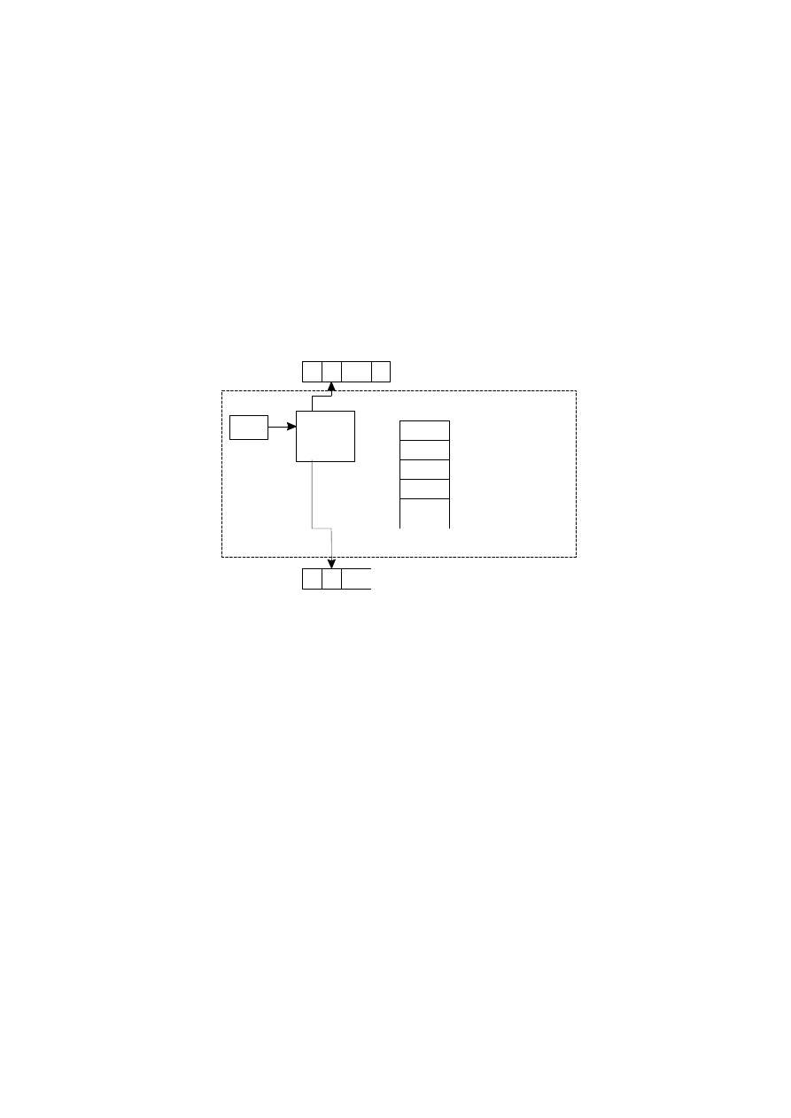
Random Access Stored Program Machine

Since the program is not stored in the memory of RAM, the program cannot modify itself.
Let us consider another model of computers called Random Access Stored Program
Machine – RASPM (Aho, Hopcroft, Ullman, 1975; Lewis, Papadimitriou, 1981). This model
is similar to RAM with the exception that the program is stored in memory and so it can
modify itself (see Figure 3). The instruction set for the RASPM is identical to the set for the
RAM, except that indirect addressing is not needed because the program can modify itself,
thus indirect addressing can be emulated.

C

P

U

In

s

tru

c

tio

n

p

o

in

te

r

M

e

m

o

ry

w

ith

p

ro

g

ra

m

..

.

r

1

r

2

r

3

r

0

A

c

c

u

m

u

la

to

r

x

x

x

1

2

n

...

y

y

1

2

...

In

p

u

t

ta

p

e

O

u

tp

u

t

ta

p

e

Figure 3: Random Access Stored Program Machine

It is not surprising that the difference in complexity between a RAM program and the
corresponding RASPM program appears only as a constant factor. So, if a problem
execution can be performed by the RAM in time T(n) than it can be performed by the
RASPM in time kT(n), where k is an appropriate constant (Aho, Hopcroft, Ullman, 1975;
Lewis, Papadimitriou, 1981):

Theorem 1.1.: If costs of instructions are either uniform or logarithmic, than for every RAM
program with time complexity T(n) there is a constant k and there is an equivalent RASPM
program with time complexity of kT(n).

Theorem 1.2.: If costs of instructions are either uniform or logarithmic, than for every
RASPM program with time complexity of T(n) there is a constant k such that there is an
equivalent RAM program with time complexity of kT(n).

EICAR 2000 Best Paper Proceedings

200

Turing Machine

The Turing Machine – TM (Aho, Hopcroft, Ullman, 1975; Lewis, Papadimitriou,
1981; Salomaa, 1985; Hopcroft, Ullman, 1979) is based on a finite automata. It means that
the machine modifies its actual state while it reads from and writes to the attached tape.
The machine accept the input string if and only if all of input symbols have been read and
the machine has entered the accepting state. There are different formal definitions of the
Turing-machine in the literature. In this work the following definition have been used (Aho,
Hopcroft, Ullman, 1975):

Definition 1.2.: Formally the T single-tape TM can be defined by the seven-tuple:

T = < Q,S,I,d,b,q

0

,q

f

>

where

•

Q is the set of states.

•

S is the set of tape symbols.

•

I is the set of input symbols; I Í S.

•

b

∈

S \ I, is the blank.

•

q

0

is the initial state.

•

q

f

is the final (accepting) state.

•

d is the set of move functions, maps a subset of Q x S to Q x ( S x {l,r,s} ).

Initially the actual state of the TM is q

0

. The actual state can be modified by the move

functions depending on the previous state and the contents of the tape. The head of the
tape can move according to the move function. It can move one cell to left or to right, or it
can stay as well.

The TM can consist of more tapes, but the computing capacity is polynomially related to
the original single-tape TM. It is possible to emulate a multitape TM using a single-tape
TM (Aho, Hopcroft, Ullman, 1975; Lewis, Papadimitriou, 1981, Regan, 1993).

Theorem 1.3.: Computing capacity of a Turing machine and a RASPM are equal, and their
expenses are comparable at polynomial level, if costs of instructions are either uniform or
logarithmic.

Although the TM is an universal tool in computing science, but it cannot do everything.
There are a lot of problem where the TM cannot be used to get the solution. Let us
consider the Church-theorem, if an algorithm exists for the solution of a problem, then this
problem can be solved by the TM as well. One of the well-known unsolvable problems is
the stopping problem of TM (Aho, Hopcroft, Ullman, 1975; Lewis, Papadimitriou, 1981):

Theorem 1.4.: It is impossible to create a TM to determine if a given TM will stop or not
using a specific input.

EICAR 2000 Best Paper Proceedings

201

RASPM with Attached Background Storage

The well-known models described above are limited to analyse only a single algorithm or
program. However, the connection between two or more algorithms or programs cannot be
examined only with much effort. In order to create connections between programs a
specific area or tape is required in which programs or program data can be stored. Let us
call that as background storage tape. Furthermore, let us suppose that all running
programs can access, read or modify this tape.

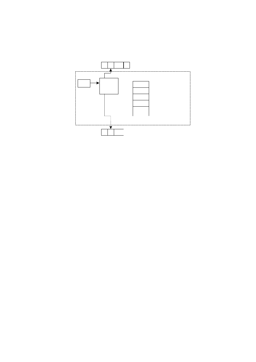
Definition 2.1.: A G Random Access, Stored Program Machine with Attached Background
Storage (called RASPM with ABS) is defined by the six-tuple:

G = < V,U,T,f,q,M >

where

•

V is a non-empty set of input symbols, output symbols and symbols stored on the
background storage tape, furthermore, a set of the symbols stored in the memory
cells (all together the tape alphabet);

•

U is a non-empty subset of the operation codes, U

⊆

V ;

•

T is a non-empty set of the possible activities of the processor;

•

f is an unique function for which f: U

→ T is true;

•

q is the initial value of instruction pointer;

•

M is the initial content of the memory.

Let us assume that an unique, one-to-one mapping is available between the V tape
alphabet and the set of integer numbers. (This way, one-to-one correspondence exists for
the input and output tapes as well as the symbols contained in memories of RASPM with
ABS or RAM).

C

P

U

In

s

tru

c

tio

n

p

o

in

te

r

M

e

m

o

ry

w

ith

p

ro

g

ra

m

..

.

r

1

r

2

r

3

r

0

A

c

c

u

m

u

la

to

r

x

x

x

1

2

n

...

y

y

1

2

...

z

z

1

2

...

In

p

u

t

ta

p

e

B

a

c

k

g

ro

u

n

d

s

to

ra

g

e

ta

p

e

O

u

tp

u

t

ta

p

e

Figure 4: Scheme of RASPM with ABS

Figure 4 shows that RASPM with ABS has an input tape, an output tape and a background
storage tape, and all of them have infinite length. The input tape can be used only for
read, the output tape only for write and the background storage tape for both operations.
The tapes can be accessed by the reading and writing heads. When reading in or writing

EICAR 2000 Best Paper Proceedings

202

out a symbol, the corresponding head moves one step to the right. In the case of
background storage, direct move of the reading/writing head is also possible. This way, we
can define the tape alphabet as identical set of integer numbers.
In addition, the machine contains a memory of infinite length, too. In contrast to the tapes,
the memory can be addressed directly (i.e. can be read in or written out directly). The first
cell of the memory has special feature, and it is called accumulator, similarly to RAM.

Operation

Parameter

Op.Code

Meaning

LOAD

operand

10

It loads the value specified by the operand to the
accumulator.

STORE

operand

20

It copies the value stored in the accumulator to the cell
specified by the operand.

ADD

operand

30

It adds the value specified by the operand to the
accumulator.

SUB

operand

40

It subtracts the value specified by the operand from the
accumulator.

MULT

operand

50

It multiplies the accumulator by the value specified by the
operand.

DIV

operand

60

It divides the accumulator by the value specified by the
operand.

AND

operand

70

It performs a bit-by-bit AND operation on the accumulator
and the value specified by the operand.

OR

operand

80

It performs a bit-by-bit OR operation on the accumulator
and the value specified by the operand.

XOR

operand

90

It performs a bit-by-bit XOR operation on the accumulator
and the value specified by the operand.

READ

operand

A0

It loads a value from the input tape to the cell specified by
the operand.

WRITE

operand

B0

It writes the value of the cell specified by the operand to
the output tape.

GET

operand

C0

It loads a value from the background storage tape to the
cell specified by the operand.

PUT

operand

D0

It writes the value of the cell specified by the operand to
the background storage tape.

SEEK

operand

E0

It moves the writing/reading head of the background
storage tape to the position specified by the operand.

JUMP

label

FC

It sets the instruction pointer to the value specified by the
label.

JGTZ

label

FD

It sets the instruction pointer to the value specified by the
label, if the accumulator contains positive number.

JZERO

label

FE

It sets the instruction pointer to the value specified by the
label, if the accumulator has been set to zero.

Figure 5: The instruction set of the RASPM with ABS

EICAR 2000 Best Paper Proceedings

203

Within the RASPM with ABS, the tape and memory handling is carried out by the
processor. Let us consider the finite set U

⊆

V. The function f maps one and only one

activity from T to each element of U. The activity f(x) that belongs to the operation code x

∈

U is a command. In the RASPM with ABS, the operation code (or command) existing
under the address determined by the instruction pointer is executed by the processor and
then the new value of the instruction pointer is set. The operation code is in a single
memory cell, and the parameter of this operation code is in the following cell. Accordingly,
a command of RASPM with ABS is stored in two cells: the first cell contains the operation
code and the second one contains the related parameter. The possible commands, thus,
the T possible activities of the processor can be seen on the Figure 5.

Let us denote the content of the ith memory cell by c(i), where i is an integer number. The
allowed operands can be seen on the Figure 6.

Operand

Operand code

Meaning

i

1

i

[i]

2

c(i)

[[i]]

3

c(c(i))

Figure 6: Operand types

Since a program can modify itself in the case of the stored program machine (RASPM),
the commands with [[i]] type operands can be substituted by the other commands,
moreover, several operations can also be substituted by a series of other operations, too.

Of course, not all possible operands can be assigned to each operation. If the destination
of an instruction has been specified by the operand then the allowed types of the operand
are [i] and [[i]]. For example, the operation READ can have operands of type [i] or [[i]] only.

The instruction set of the RASPM with ABS and the code belonging to each operation are
included in Figure 5, too. The hexadecimal code of operation is defined by two digits. The
first digit refers to the operation, and the second digit refers to the type of operand. It
means if the parameter of an instruction is an operand then the instruction code can be
calculated by adding the operation code and the operand code.
When the instruction pointer addresses memory cell(s) where the content is an x

∈

V and x

∉

U, (i.e. it is not an operation code, there is no command assigned to it) the machine

stops.

When the machine is switched on, the instruction pointer takes the initial q value and the
processor executes the command addressed by the q value immediately. The program
and algorithm to be executed will be determined by commands existing in the memory,

EICAR 2000 Best Paper Proceedings

204

therefore, it should be determined by the initial content of the memory (M). The machine
stops in the following cases:

•

when it is switched off,

•

when it has got a value of the cell specified by the instruction pointer and this value
is not an instruction code,

•

when a division by zero should be executed.

In contrast to RAM, therefore, there is no command to stop the machine. (In addition to the
division by zero, of course, it is possible to create an infinite loop when no operation is
performed).

The content of memory is the initial value of M at every switching on and it is deleted at
every switching off. On the contrary, the background storage keeps its content also at
switching off. Eventually, it may happen that the background storage is removed from the
machine and attached to another machine for further use. It is an other obvious advantage
that the RASPM with ABS can be extended because it can be attached to more
background storage tapes at the same time. The Random Access Stored Program
Machine with Several Attached Background Storage can be defined on the base of original
RASPM with ABS. Only a new command must be defined:

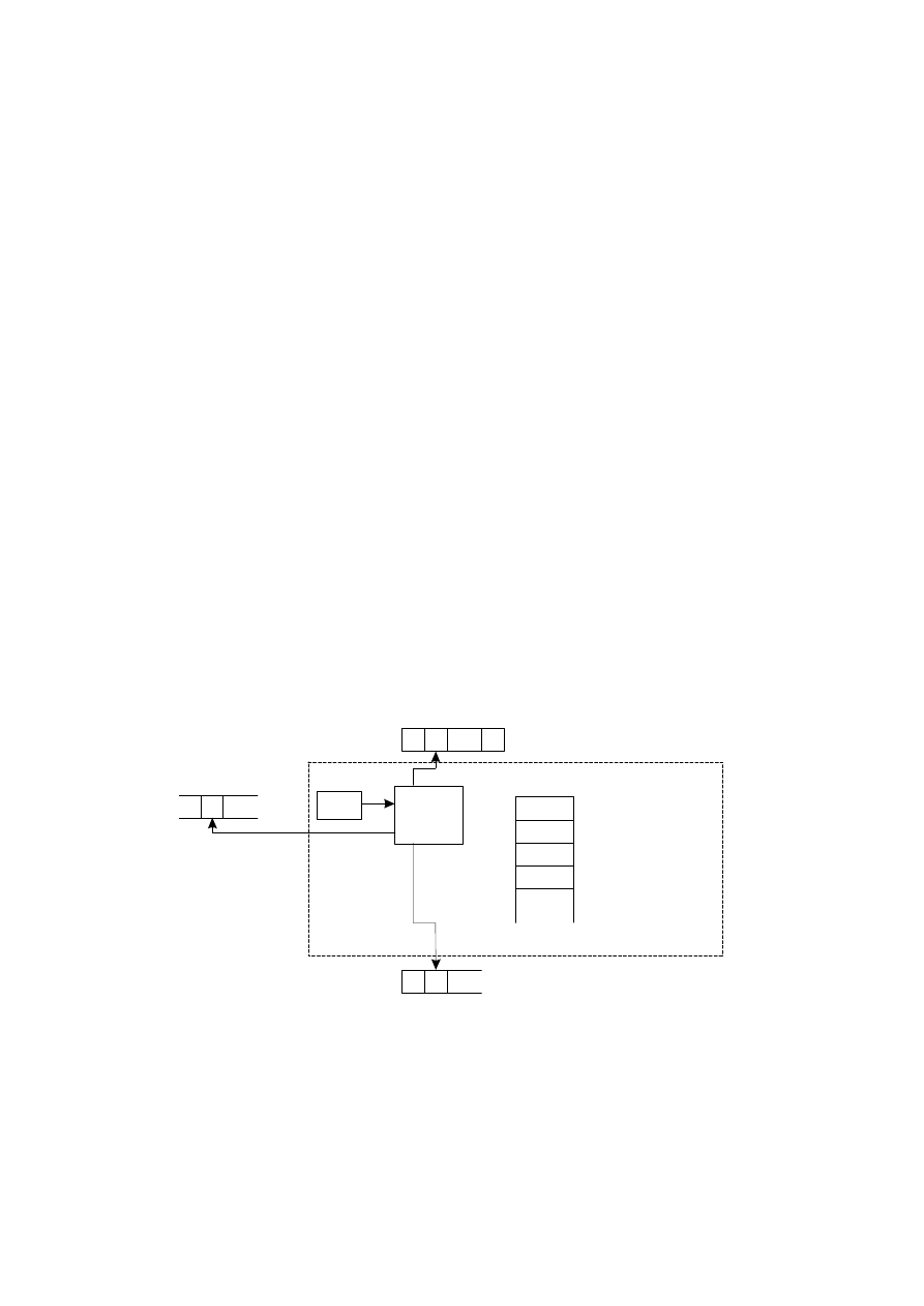
Definition 2.2.: The Random Access Stored Program Machine with Several Attached
Background Storage (RASPM with SABS) is defined as a RASPM with ABS with the
following extensions:

•

A RASPM with SABS can be attached to more background storage tapes at the
same time.

•

All symbols of all background storage tapes are in V.

•

The possible activities of the processor T is extended by one activity. The actual
background storage tape can be selected by this new command (Figure 7).

•

After the execution of this command, every operation referring to the background

storage tape is performed on the actual background storage tape.

•

If a command relating to a background storage tape is performed without giving a
SETDRIVE command previously, then this command will use the first background
storage tape.

•

The machine stops when a RASPM with ABS stops, furthermore if a SETDRIVE
command relating to an invalid background storage tape would be performed.

EICAR 2000 Best Paper Proceedings

205

Operation

Parameter

Op.Code

Meaning

SETDRIVE

operand

F0

It sets the actual background storage tape to a new
one specified by the operand.

Figure 7: New operation in RASPM with SABS

Theorem 2.1.: The RASPM with SABS is equivalent to RASPM with ABS, so one can be
simulated by the other one.

Proof: It is enough to prove that a RASPM with SABS can be simulated by the RASPM
with ABS, since the opposite case is trivial. Let us comb the N tapes of the original,
simulated machine (RASPM with SABS) to the single tape of the simulating machine
(RASPM with ABS) by the following way: The tapes of the simulated machine are
numbered from 0 to N-1. Let the jth symbol of the ith tape be transferred to the Nj+i-th
position on the new tape. Let us modify the memory building of the simulating machine as
follows:

•

the cell 0 is the accumulator,

•

the cell 1 is kept for further purposes,

•

the cell 2 contains the address of the cell (from 3 to N+2) that contains the location
of the reading/writing head of the background storage tape,

•

the cell i (3

≤

i

≤

N+2) contains the position of the reading/writing head of the i-3th

virtual background storage tape,

•

the cell i (N+2<i) contains the content of the cell i-(N+2) of the simulated machine, if
that has not been modified otherwise it is shifted, see below.

The commands of the simulated machine has to be copied into the memory of the
simulating machine, but the following modifications should be achieved:

•

If the original program has to modify the actual background storage tape, the
sequence number of the new tape gets into the cell 2. In this case, instead of the
original command SETDRIVE a the following commands should be deposited:

STORE

[1]

; Save the accumulator

LOAD

a

; Load the operand

ADD

3

; calculate the real address

STORE

[2]

; save it as the new actual tape

LOAD

[1]

; Restore the accumulator

•

If the original program reads or writes the actual background storage tape, the head
of the single background storage tape moves to the actual position. Now the
required operation can be performed and the position of the head of actual
background storage tape is modified. The appropriate commands for a write
operation (PUT a) are as follows:

EICAR 2000 Best Paper Proceedings

206

STORE

[1]

; Save the accumulator

SEEK

[[2]]

; Move the head

PUT

a

; Write the operand to the tape

LOAD

[[2]]

; Load the position of the actual head

ADD

N

; modify the position

STORE

[[2]]

; Save new position

LOAD

[1]

; Restore the accumulator

•

If the original program modifies the position of the reading/writing head of
background storage tape (SEEK a), then the simulating program performs the
change in the appropriate cell as follows:

STORE

[1]

; Save the accumulator

LOAD

a

; Load the operand

MULT

N

; Calculate the operand

ADD

[2]

; to the real

SUB

3

; position on the tape

STORE

[[2]]

; Save the new position

LOAD

[1]

; Restore the accumulator

•

In the course of copy of the original program the memory cell references should be
also translated according to the shifts being in the program of the simulating
machine.

In such way we could simulate a RASPM with SABS with the help of a RASPM with ABS
by substituting several commands with a series of other commands. Not more than 7 other
commands are necessary for the simulation of each command to be simulated. Therefore,
on the basis of the uniform cost criterion, if the time complexity of the simulated program is
T(n), then the time complexity of the simulating program is not more then 7T(n). This is
valid independently on the input. If we consider a logarithmic cost criterion, the situation
becomes much more complicated. In such case, the cost of STORE [1] and LOAD [1]
commands is a function of the initial content of the accumulator. However, it is clear that
the content of the accumulator has to be produced by the original program as well, and
this production has also logarithmic cost with similar function of the size of the
accumulator. It means that the commands STORE [1] and LOAD [1] can increase the
logarithmic cost of the original program by a constant multiplication factor only, even in the
worst case. The above program details for simulation of commands contain some such
commands that perform operations with the operand of the original command or with its
value multiplied by a constant factor. (Here it is supposed that the N number of tapes can
be considered as a constant). Consequently, the logarithmic expense T(n) of the original
program is increased to cT(n) only.

Therefore the computing capacity of the RASPM with ABS cannot be increased by using
more background storage tapes. After understanding these facts it is not surprising that
the computing capacity of RASPM with ABS is not greater than that of RASPM as follows:

EICAR 2000 Best Paper Proceedings

207

Theorem 2.2.: Any RASPM with ABS can be simulated by a RASPM, and the cost
functions of the simulating program agree with the cost function of the simulated program
multiplied by an appropriate constant factor.

Proof: Similarly to the proof of Theorem 2.1., let us comb now, the content of the memory
and the background storage into a new memory. Then a RASPM is obtained, i.e. a
machine without background storage. The main difference in combing is that the original
memory has to be shared into blocks, because the combing may not cut the cells
belonging to one instruction. Of course, a new JUMP instruction has to be appended to the
end of each block. In this way the original program code can be transferred into the new
memory and the content of the background storage can be inserted between the program
blocks. In the course of transfer of the original program, the memory cell references should
be also translated according to the shifts being in the program of the simulating machine.
The other difference in combing is that now, there is no need for cell to contain the
sequence number of the actual background storage (because the RASPM with ABS
contains only one), moreover, that only one cell is required to contain the position of the
unique reading/writing head.

A conclusion of Theorem 2.2. is the following:
Theorem 2.3.: Computing capacity of a Turing Machine and a RASPM with ABS are equal,
and their expenses are comparable at polynomial level.

Proof: Since any RASPM with ABS can be simulated by a RASPM (Theorem 2.2.) and vice
versa (it is trivial), moreover, any RASPM can be simulated by a Turing Machine, and vice
versa (Theorem 1.3.), therefore a RASPM with ABS can also be simulated by a Turing
Machine and vice versa. The cost criterion follows from the statement in Theorems 1.3.
and 2.2.

The background storage of RASPM with ABS can be regarded as an input and an output
tape together, since it is assumed that there are already data for input on the background
storage when the machine starts and that the storage can contain data after the switching
off the machine as well. In the RASPM the role of background storage can be taken by the
input tape over that the input tape contains the content of the background storage as well.
It can be accomplished by assigning the cells with even sequence numbers of the tape to
the cells of the original input tape, and the cells with odd sequence numbers to the cells of
background storage. At switching on the machine, the RASPM copies the first amount of
cells from the input tape into the free memory cells existing between the program blocks
which memory sharing was introduced in the proof of Theorem 2.2. This copy can be
executed so that the copying procedure deposits data only into the even cells between the
program blocks. (The odd cells will be used as temporary output tape.) While the program
is running and such input or background tape referred instruction should be performed that
data has not been entered yet then the machine reads and stores automatically the
suitable amount of following cells from the input tape till it reaches the required data.
When the program tries to write into a cell of the virtual background storage then it writes
to the appropriate position of the memory. Of course, if the referred cell has not been read

EICAR 2000 Best Paper Proceedings

208

yet then it has to be read previously. When the program tries to write onto the output tape
then it writes to the next free odd cell between the program blocks. Before the RASPM
stops, it deposits the content of the background storage and the virtual output tape onto
the real output tape. In this sense the RASPM can also be regarded as a machine
equipped with a background storage.

Operating systems' model

We should like to use the RASPM with ABS and the RASPM with SABS for the execution
of programs. The V, U, T, and f components of G = < V,U,T,f,q,M > have been defined
previously after the definitions 2.1. and 2.2. Now, if we specify q and M, a program can be
given which is specific for the operation of the machine. There are program and data files
on the background storage(s). Via the input tape we should like to decide the running
sequence of programs. A running program is allowed to read, write or modify also a
background storage including the existing program and data files. Therefore, a frame
program is required which is able to handle the program and data files and makes the
specified program code run.

Definition 3.1.: The operating system is defined as a system of programs, which is able to
handle separate program or data files and makes a specified program run.
Giving the definition of the operating system of the RASPM with ABS, the similarity
between the RASPM with ABS and the real computer systems can be observed. In both of
these systems there is a background storage where the user can store separate data and
program files. Furthermore, there is an operating system which is able to handle these
files.

The operating system can be included either in the initial value M of the memory or it can
be located in the background storage. In the latter case, the M initial value of the memory
contains a specific program started at the place specified by q which loads the operating
system from the background storage and makes it run. In this case the loading program is
not considered as part of the operating system.

Definition 3.2.: If the M initial value of the memory contains the operating system, then this
operating system is called as machine specific operating system.

It means that by specifying the RASPM with ABS the operating system is also defined,
because the M (with the code of the operating system) is specified by the RASPM with
ABS.

Definition 3.3.: If the operating system is contained by the background storage tape, then
this operating system is called as machine independent operating system.

In this case the operating system of a RASPM with ABS can be changed easily. The only
thing to do is to change the actual background storage tape.

EICAR 2000 Best Paper Proceedings

209

On the other approach, the machine can be operating system specific or operating system
independent:

Definition 3.4.: If the M initial value of the memory in a RASPM with ABS contains the
operating system, then this machine is called as operating system specific machine.

In this case the machine can use its own operating system only. (Of course, it is possible
to create a program which can simulate another operating system.)

Definition 3.5.: If the operating system of a RASPM with ABS is contained by the
background storage tape, then this RASPM with ABS is called as operating system
independent machine.

Of course, it is possible to change the background storage tape and the operating system
as well.

The following theorems are direct conclusions of the definitions 3.1-3.5.:
Theorem 3.1.: If O is the machine specific operating system of the G RASPM with ABS
then G is operating system specific machine.

Proof: It is trivial, because if O is the machine specific operating system of the G machine
then the memory of G contains the O operating system. It means that G is operating
system specific machine.

Theorem 3.2.: If O is the machine independent operating system of the G RASPM with
ABS then G is operating system independent machine.

Proof: It is also trivial, because if O is the machine independent operating system of the G
machine then the memory of G does not contains the O operating system, but the
background storage tape includes O. It means that G is operating system independent
machine.

According to the general requirements summarized also by an ISO standard, the operating
system is a program system which manages the execution of programs: schedules the
execution, shares the resources and makes the connections between unique programs.

In practice, the operating system concept is based upon tradition. Main parts of operating
systems (Deitel, Lorin, 1981; Herzog, Kollland, 1994; Dewan, Vasilik, 1990) have to be
included in every multitasking operating system. The mechanism described under the 3rd
point can be left out in the case of non-multitasking operating system.

According to the definition 3.1., the operating system of the RASPM with ABS can be
defined for the purpose of examining the connection between unique program codes.
Using the RASPM with ABS, the operating system complying with the requirements
described above can be defined independently on being the RASPM with ABS operating

EICAR 2000 Best Paper Proceedings

210

system specific or not. However, if we would like to examine program codes that modify
the code of the operating system then operating system independent machine should be
used. Otherwise, the operating system can not be really modified, because the restarting
of the machine always clears the occasional modifications.

Viruses in RASPM with ABS

The concept of operating system has been defined in 3.1 as a system of programs able to
handle and make run program files. Therefore the definition of the viruses in RASPM with
ABS can also be given:

Definition 4.1.: A computer virus is defined as a part of a program which is attached to a
program area and is able to link itself to other program areas. The code of computer virus
has to be executed when that program area is to be executed which the virus has been
attached to.

Viruses have not to execute the original part of the program area, but the viruses often do
it because they want to be unobserved. In this case the original part of the program area
has to be repaired by the virus. In the opposite case the virus may overwrite the program
area thus the virus destroys it.

Spreading modes of viruses

As it is known in the practice, a virus can be attached to various program areas. The forms
of attachment to different program areas are called as spreading modes. Viruses can have
different spreading modes.

Definition 4.2.: A spreading mode of a virus is called machine-specific when some
characteristic feature or service of the machine is used by the virus when it is spread by its
given spreading mode. When the services of the machine are not used by the virus when
it is spread then the spreading mode is called machine-independent.

A spreading mode of a virus can be machine-specific for instance when the program areas
which can be infected by the virus are depending on the machine. For example in the case
of IBM PCs the boot viruses have machine specific spreading mode, because boot sector
layout depends on the structure of the IBM PC. Any boot virus under IBM PC has to use
the service of the BIOS or the disk controller for its spreading.
A spreading mode of a virus can be machine-independent for instance when the program
areas which can be infected by the virus are not depending on the machine. For example
the viruses which can infect C source file have machine-independent spreading mode,
because they can infect C source files under different machines using the same spreading
mode.

Similar definitions holds for the dependency of spreading modes from the operating
system:

EICAR 2000 Best Paper Proceedings

211

Definition 4.3.: The spreading mode of a virus is called operating system-specific when
some characteristic feature or service of the operating system is used by the virus when it
is spread by its given spreading mode. When the services of the operating system are not
used by the virus during its spreading, the spreading mode is called operating system-
independent.

A spreading mode of a virus can be operating system-specific for instance when the
program areas which can be infected by the virus are depending on the operating system.
For example under the DOS operating system viruses that infect .EXE files have DOS
specific spreading mode, because the structure of the .EXE files is DOS specific.

A spreading mode of a virus can be operating system-independent for instance when the
program areas which can be infected by the virus are not depending on the operating
system. For example under the DOS operating system the boot viruses usually have DOS
independent spreading mode, because the infection of boot sector (or master boot sector)
can be performed without using DOS services.

Definition 4.4.: The virus is called machine-specific when it can be spread only by
machine-specific spreading mode, and the virus is called machine-independent if its all
spreading modes are machine-independent.

Definition 4.5.: The virus is called operating system-specific when it can be spread only by
operating system-specific spreading mode, and the virus is called operating system-
independent if its all spreading modes are operating system-independent.

It is obvious that executable program files can not be infected by a really machine-
independent virus since it has to use the instruction set of the interpreter which can
execute the executable file. The executable files are generated from source files written in
a high level programming language. A virus can modify these source files during its
spreading, thus the virus is independent from the processor which executes the virus
code. Of course, the compilers which compile the source codes have to be compatible to
each other.

The boot viruses of IBM PCs are machine-specific, but operating system-independent
viruses. The file append viruses under DOS operating system which infects executable
files are machine-specific and operating system-specific viruses and the file append
viruses under DOS operating system which infects source files are machine-specific and
operating system-specific viruses.

Definition 4.6.: The spreading mode is called direct when the virus is attached to an
executable file during its spreading, and indirect, when the virus is attached to a non-
executable file during its spreading.

EICAR 2000 Best Paper Proceedings

212

In the case of viruses with direct spreading mode the virus infects executable files. The
executable files can be interpreted by the operating system or by the other program. For
example the Microsoft Word for Windows 6.0 documentation file which can include a
macro program is an executable file, because the Word can interpret and execute the
macro program. Thus a virus can infect these documentation files and this is direct
spreading mode as well.

In the case of viruses with indirect spreading mode the viruses have to infect source files.
These source files have to be compiled and/or linked. It means that the viruses can appear
in the executable files in different forms, depending on the compiler and the linker. In such
cases the virus fully build in the host program.

Oligomorphic and Polymorphic Viruses

The form of appearance of the viruses discussed above are the same in all occasion of
infection. However, it is easy to imagine that a virus can change its own form in some ways
during the infection.

Definition 4.7.: The spreading mode is called polymorphic when there are two program
areas infected by the specified spreading mode of the same virus and the code sequences
of the virus programs are different.

Definition 4.8.: The virus is called polymorphic when it has polymorphic spreading mode.

Definition 4.9.: The spreading mode is called oligomorphic when there are two program
areas infected by the specified spreading mode of the same virus and the code sequences
of the virus programs are the same, but there are at least one part of the virus code which
is crypted by different keys.

Definition 4.10.: The virus is called oligomorphic when it has oligomorphic spreading mode
and it has not polymorphic spreading mode.

A possible realisation of oligomorphic viruses is a special copy when the virus uses a
method of cryptography with a random key. An oligomorphic virus attaches also a
decoding part to the encoded virus program.
The realisation of polymorphic viruses is more complicated than oligomorphic viruses.
They can change their encoding part, too. This is possible e.g. by a random selection of
encoding routines from prepared set. This method can also be performed by a random
generation of the routine´s commands during the spreading. It can be realized e.g. by the
following ways:

•

by changing the sequence order of the encoding routine,

•

by using that the processor is able to perform the same operation by more than one
command or command sequences,

•

by putting dummy commands in the encoding routine randomly.

EICAR 2000 Best Paper Proceedings

213

In the practice there are some subtypes of oligomorphic and polymorphic viruses:
Definition 4.11.: The virus is called slow-polymorphic when it has polymorphic spreading
mode, but it uses the polymorphism very rarely.

Definition 4.12.: The virus is called slow-oligomorphic when it has oligomorphic spreading
mode, but it changes the random key of the coder routine very rarely.

The Virus Detection Problem

With the emergence of viruses the problem of virus detection also emerges:
Definition 5.1.: The virus detection problem is a question of theory of algorithms, namely
whether a specific algorithm exists or not which is able to decide that a specified program
area contains a virus able to be spread or not.

Here we assume that all information is available concerning the format of the program
area. It means that in the case of an executable file the instruction set of the processor
and the operation of each command is known; in the case of source files the syntax of the
programming language and the operation of the compiler is fully known.

The General Problem of Virus Detection

Considering the Church-theorem (Aho, Hopcroft, Ullman, 1975; Lewis, Papadimitriou,
1981; Salomaa, 1985), if there is an algorithm which is able to solve the virus detection
problem, then a Turing-machine can be built to execute the corresponding algorithm.
Unfortunately it is impossible to build such a Turing-machine even in the simplest case:
Theorem 5.1.: It is impossible to build a Turing-machine which could decide if an
executable file in a RASPM with ABS contains a virus or not.

Proof: According to theorem 1.3. it is possible to create a RASPM or RASPM with ABS to
simulate the Turing-machine. (The modification of the expenses functions of the
procedures due to the simulation is irrelevant from the point of view of the proof of the
theorem.) Therefore let us create a program P in the RASPM with ABS which simulates
the Turing-machine. This program writes a character 1 onto the output tape when the
simulated Turing-machine stops in an acceptable state.
Let us make an easy virus which is able to infect program files. Let the virus contain the
mentioned program P in such way that at first P is executed as an answer for a random but
fixed B input, then the virus starts running. It can be realized by attaching the virus to P,
and inserting a JUMP command after each "write character 1" command of P. Thus the
control is passed to the first command of the virus program. Let the virus program be so
that it copies not only the virus program but also the program P and the fixed input B as
well, in the event of infection.

According to this procedure, it is possible to create a program V in RASPM with ABS for
any Turing-machine, that becomes a virus if it is really able to be spread. It is obvious that

EICAR 2000 Best Paper Proceedings

214

program V can spread if program P and consequently the Turing-machine stops for the
fixed input.

Let us suppose the opposite: there exists a Turing-machine T, which reads any program of
RASPM with ABS and writes the character 1 out if the program contains a virus and writes
the character 0 out if it does not. If the Turing-machine answers the input program V by the
character 1 then program P or the corresponding Turing-machine will stop receiving the
input B in any case. If the answer is 0, the corresponding Turing-machine will never stop.
Therefore the Turing-machine is able to decide that an other Turing-machine will or will
not stop as an answer for any input. However, this is impossible (Salomaa, 1985, Leitold,
Csótai, 1992)

o.

The conclusion is the following: According to the Church theorem there is no way to build
an algorithm for the detection of viruses.

Now, we see that the virus detection problem defined by definition 5.1. cannot be solved.
Therefore, it is advisable to restrict the problem.

Virus Detection Methods

A possible simplification of the virus detection problem if we deal with "several" known
viruses only. In this case the known viruses can also be used for the detection algorithm.

Let us take a series of codes from each known virus, which emerges in every infected file
when an infection takes place. Let be this series of codes called as sequence. The task of
the virus detection program is reduced to the search for these sequences in the program
areas. Further problems emerge, however, concerning the algorithms of this principle:

•

It is not for sure that there are some sequences for a polymorphic virus that can
detect all variants of the virus.;

•

It is unknown what is the probability of false alarms, i.e. when a sequence is found
by random;

•

It is a question what kinds of expenses criteria are suitable to the realisation of the
sequence searching algorithm.

It is obvious that the method can not be used for detection of polymorphic viruses and we
have to look for other procedures for this purpose, but the method can be used for
oligomorphic viruses as well. In this case the sequence for searching should be generated
using the codes of decoder function of the virus.

The quantity of false alarms depends on the length of the sequences and on the
probability of finding specified values in specified cells of the program files. If the length of
a sequence is N, maximum n values can appear at equal probability, there are altogether
M sequences and the overall length of the examined files is L >> N, then the probability of
finding any of the sequences in a file is:

EICAR 2000 Best Paper Proceedings

215

p

L M

n

N

≈ ⋅ ⋅

1

.

Let us examine now the expenses criterion with which the sequence searching algorithm
can be realized. Since computers often used in practice have fixed length of cells and
memory size (which is not the case for RASPM with ABS), the expense of each command
will be less than a constant value. It is recommended therefore to calculate with uniform
expenses. The sequence searching algorithm compares the content of each cell to be
examined with the first cells of the sequences. If the examination is executed separately,
altogether

L M

⋅

comparisons have to be performed. However, the sequences can be

ordered according to the content of their first cells. Let us start the examination with the
character in the middle position, and then follow the procedure into the right direction.
Using this method in average only

L

M

⋅

log

comparisons have to be carried out,

provided the contents of the first cells of sequences are different ones (



x



denotes the

integer number not less then x ). If identical values are found in the first cells of the
sequences, the contents of the 2nd cells have also to be examined. The expected value of

the required further examinations is

L M

n

⋅ ⋅

1

, therefore this is the number of the

examinations required in addition. If there is an identity found in the kth examination,

further

L M

n

k

⋅ ⋅

1

examinations are required. Therefore, the expected value of the

altogether required examinations is:

1

1

1

1

1

...

1

1

1

1

2

−

−

⋅

⋅

=













+

+

+

+

⋅

⋅

=

−

n

n

M

L

n

n

n

M

L

s

N

N

Considering the worst possible case, the maximum number of comparisons is s

L M N

= ⋅ ⋅

.

Since the time requirement of the algorithm can be estimated by the number of
comparisons, therefore the sequence searching algorithm can be realized in polynomial
time.

For identification of polymorphic viruses a simulation method can be used. The substance
of the method is that the execution of the examined program file is started during the
emulation (simulation) of the processor. A statistics is prepared about the executed
commands, which is continuously compared to the existing statistics of known polymorphic
viruses. When an agreement is found, a virus is detected. Based on this method, after
encoding, the operation codes of the suspected program can be investigated. Compared
to the sequence searching process, no part of the series of codes is compared to known
codes, but a statistics prepared from the operation codes of a certain part of code series is
examined. In such a way the viruses can be identified even if parts of the commands are
exchanged. However, in order to reach a safety of the search comparable to the sequence
search method the statistics has to be based on much more operation codes.

EICAR 2000 Best Paper Proceedings

216

However, the emulation type searching method can not be realized within polynomial time,
since a virus can exist decoding routine of which is executed in exponential time,
depending on a random number. A possible method of searching unknown viruses is the
processor emulating method mentioned for the polymorphic viruses. In this case, however,
no statistics is prepared, but a characteristic virus activity is watched. These typical
characteristic virus activities are, e.g. when a program

•

modifies an other program file,

•

attempts to modify an other program file,

•

attempts to modify the operating system.

Conclusion

This paper highlighted a new computation model of operating systems. Using the defined
RASPM with ABS/SABS it is very easy to examine the working mechanism of unique
programs interacting other program codes under different operating systems. This
interaction can be carried out that the unique program codes can be identified on the
background storage. This identification and also the handling are carried out by operating
systems thus operating systems must be previously defined. This definition was given in
the 3

rd

point of this paper which complies with the general requirements. The RASPM with

ABS/SABS with the operating system together is a powerful tool for the examination of
interacting algorithms (program codes) which are under the influence of each other,
moreover, which can be modified by the other such as computer viruses.
Under the new model the definitions of computer viruses and the spreading modes of
computer viruses is provided. It is proved that the general virus detection problem can not
be solved. It means that the virus detection problem should be simplify until it can be
solved by an algorithm and therefore can be used in practice.
In the last part of this paper two virus detection method used in practice is provided. The
sequence searching algorithm can be solved in polynomial time, but this method can not
be used for detection of polymorphic viruses. The other method is the simulation method
which can be used for detecting the polymorphic viruses as well, but this searching
method can not be realized within polynomial times in all cases.

EICAR 2000 Best Paper Proceedings

217

References

Aho, A. V.; Hopcroft, J. E.; Ullmann, J. D. (1975). The design and analysis of computer
algorithms, Addison-Wesley.

Davis, M. (1958). Computability and Unsolvability, McGraw-Hill, New York.

Lewis, H; Papadimitriou, C. (1981). Elements of the theory of computation, Prentice-Hall,
New Jersey

Salomaa, A. (1985). Computation and Automata, Cambridge University Press.

Hopcroft, J. E.; Ullmann, J. D. (1979). Introduction to Automata Theory, Languages and
Compilation, Addison-Wesley.

Regan, K.W. (1993). On the difference between Turing machine time and random-access
machine time, Proceedings of the ICCI'93, Fifth International Conference on Computing
and Information, 27-29 May 1993, Sudbury, Canada, pp. 36-40.

Bshouty, N.H. (1993). On the complexity of functions for random access machines, Journal
of the Association for Computing Machinery, Vol: 40. No: 2., Apr 1993, pp. 211-223

Leitold, F.; Csótai, J. (1992). Virus Searching and Killing Language, Proceedings of the 2

nd

International Virus Bulletin Conference, 2-3 Sep 1992, Edinburgh, UK, pp. 159-172.

Virus Bulletin (1993). Survivor's guide to computer viruses, Virus Bulletin, Abingdon+.

Deitel, H. M.; Lorin, H. (1981) Operating Systems, Addison-Wesley.

Herzog, H.; Kolland, M. (1994). Requirements of future information systems on operating
system architectures, Wirtschaftsinformatik, Vol: 36 Iss: 2, 1994, pp. 117-129.

Dewan, P.; Vasilik, E. (1990). Object model for conventional operating systems,
Computing Systems, Vol: 3 No: 4 Fall 1990, pp. 517-549.