
Solution Manual for
A Course in Game Theory


Solution Manual for
A Course in Game Theory
by Martin J. Osborne and Ariel Rubinstein
Martin J. Osborne
Ariel Rubinstein
with the assistance of Wulong Gu
The MIT Press
Cambridge, Massachusetts
London, England

Copyright c
1994 Martin J. Osborne and Ariel Rubinstein
All rights reserved. No part of this book may be reproduced in any form by any electronic
or mechanical means (including photocopying, recording, or information storage and
retrieval) without permission in writing from the authors.
This manual was typeset by the authors, who are greatly indebted to Donald Knuth (the
creator of TEX), Leslie Lamport (the creator of L
A
TEX), and Eberhard Mattes (the creator
of emTEX) for generously putting superlative software in the public domain, and to Ed
Sznyter for providing critical help with the macros we use to execute our numbering
scheme.
Version 1.2, 2005/1/17

Contents
Preface
ix
2
Nash Equilibrium
1
Exercise 18.2 (First price auction)
1
Exercise 18.3 (Second price auction)
1
Exercise 18.5 (War of attrition) 2
Exercise 19.1 (Location game)
2
Exercise 20.2 (Necessity of conditions in Kakutani’s theorem)
3
Exercise 20.4 (Symmetric games)
3
Exercise 24.1 (Increasing payoffs in strictly competitive game)
3
Exercise 27.2 (BoS with imperfect information)
4
Exercise 28.1 (Exchange game)
4
Exercise 28.2 (More information may hurt) 4
3
Mixed, Correlated, and Evolutionary Equilibrium
7
Exercise 35.1 (Guess the average)
7
Exercise 35.2 (Investment race) 7
Exercise 36.1 (Guessing right)
8
Exercise 36.2 (Air strike)
8
Exercise 36.3 (Technical result on convex sets) 9
Exercise 42.1 (Examples of Harsanyi’s purification)
9
Exercise 48.1 (Example of correlated equilibrium)
10
Exercise 51.1 (Existence of ESS in 2 × 2 game)
10
4
Rationalizability and Iterated Elimination of Dominated Actions
11
Exercise 56.3 (Example of rationalizable actions)
11
Exercise 56.4 (Cournot duopoly)
11
Exercise 56.5 (Guess the average)
11
Exercise 57.1 (Modified rationalizability in location game)
11
Exercise 63.1 (Iterated elimination in location game)
12
Exercise 63.2 (Dominance solvability)
12
Exercise 64.1 (Announcing numbers) 12
Exercise 64.2 (Non-weakly dominated action as best response)
12
5
Knowledge and Equilibrium
13

vi
Contents
Exercise 69.1 (Example of information function)
13
Exercise 69.2 (Remembering numbers) 13
Exercise 71.1 (Information functions and knowledge functions) 13
Exercise 71.2 (Decisions and information)
13
Exercise 76.1 (Common knowledge and different beliefs)
13
Exercise 76.2 (Common knowledge and beliefs about lotteries) 14
Exercise 81.1 (Knowledge and correlated equilibrium)
14
6
Extensive Games with Perfect Information
15
Exercise 94.2 (Extensive games with 2 × 2 strategic forms)
15
Exercise 98.1 (SPE of Stackelberg game)
15
Exercise 99.1 (Necessity of finite horizon for one deviation property)
16
Exercise 100.1 (Necessity of finiteness for Kuhn’s theorem) 16
Exercise 100.2 (SPE of games satisfying no indifference condition)
16
Exercise 101.1 (SPE and unreached subgames) 17
Exercise 101.2 (SPE and unchosen actions)
17
Exercise 101.3 (Armies)
17
Exercise 102.1 (ODP and Kuhn’s theorem with chance moves)
17
Exercise 103.1 (Three players sharing pie)
17
Exercise 103.2 (Naming numbers) 18
Exercise 103.3 (ODP and Kuhn’s theorem with simultaneous moves)
18
Exercise 108.1 (-equilibrium of centipede game)
19
Exercise 114.1 (Variant of the game Burning money) 19
Exercise 114.2 (Variant of the game Burning money) 19
7
A Model of Bargaining
21
Exercise 123.1 (One deviation property for bargaining game)
21
Exercise 125.2 (Constant cost of bargaining)
21
Exercise 127.1 (One-sided offers) 21
Exercise 128.1 (Finite grid of possible offers)
22
Exercise 129.1 (Outside options)
23
Exercise 130.2 (Risk of breakdown)
24
Exercise 131.1 (Three-player bargaining)
24
8
Repeated Games
25
Exercise 139.1 (Discount factors that differ )
25
Exercise 143.1 (Strategies and finite machines)
25
Exercise 144.2 (Machine that guarantees v
i
) 25
Exercise 145.1 (Machine for Nash folk theorem)
25
Exercise 146.1 (Example with discounting)
26
Exercise 148.1 (Long- and short-lived players)
26
Exercise 152.1 (Game that is not full dimensional )
26
Exercise 153.2 (One deviation property for discounted repeated game)
26
Exercise 157.1 (Nash folk theorem for finitely repeated games)
27
9
Complexity Considerations in Repeated Games
29
Exercise 169.1 (Unequal numbers of states in machines)
29
Exercise 173.1 (Equilibria of the Prisoner’s Dilemma) 29
Exercise 173.2 (Equilibria with introductory phases)
29

Contents
vii
Exercise 174.1 (Case in which constituent game is extensive game)
30
10 Implementation Theory
31
Exercise 182.1 (DSE-implementation with strict preferences)
31
Exercise 183.1 (Example of non-DSE implementable rule) 31
Exercise 185.1 (Groves mechanisms)
31
Exercise 191.1 (Implementation with two individuals)
32
11 Extensive Games with Imperfect Information
33
Exercise 203.2 (Definition of X
i
(h)) 33
Exercise 208.1 (One-player games and principles of equivalence)
33
Exercise 216.1 (Example of mixed and behavioral strategies) 33
Exercise 217.1 (Mixed and behavioral strategies and imperfect recall )
33
Exercise 217.2 (Splitting information sets) 34
Exercise 217.3 (Parlor game)
34
12 Sequential Equilibrium
37
Exercise 226.1 (Example of sequential equilibria)
37
Exercise 227.1 (One deviation property for sequential equilibrium)
37
Exercise 229.1 (Non-ordered information sets) 39
Exercise 234.2 (Sequential equilibrium and PBE )
39
Exercise 237.1 (Bargaining under imperfect information)
39
Exercise 238.1 (PBE is SE in Spence’s model )
40
Exercise 243.1 (PBE of chain-store game)
40
Exercise 246.2 (Pre-trial negotiation)
41
Exercise 252.2 (Trembling hand perfection and coalescing of moves)
41
Exercise 253.1 (Example of trembling hand perfection)
42
13 The Core
45
Exercise 259.3 (Core of production economy)
45
Exercise 260.2 (Market for indivisible good )
45
Exercise 260.4 (Convex games) 45
Exercise 261.1 (Simple games)
45
Exercise 261.2 (Zerosum games)
46
Exercise 261.3 (Pollute the lake)
46
Exercise 263.2 (Game with empty core)
46
Exercise 265.2 (Syndication in a market )
46
Exercise 267.2 (Existence of competitive equilibrium in market) 47
Exercise 268.1 (Core convergence in production economy)
47
Exercise 274.1 (Core and equilibria of exchange economy)
48
14 Stable Sets, the Bargaining Set, and the Shapley Value
49
Exercise 280.1 (Stable sets of simple games)
49
Exercise 280.2 (Stable set of market for indivisible good )
49
Exercise 280.3 (Stable sets of three-player games)
49
Exercise 280.4 (Dummy’s payoff in stable sets) 50
Exercise 280.5 (Generalized stable sets) 50
Exercise 283.1 (Core and bargaining set of market )
50
Exercise 289.1 (Nucleolus of production economy)
51

viii
Contents
Exercise 289.2 (Nucleolus of weighted majority games)
52
Exercise 294.2 (Necessity of axioms for Shapley value)
52
Exercise 295.1 (Example of core and Shapley value)
52
Exercise 295.2 (Shapley value of production economy)
53
Exercise 295.4 (Shapley value of a model of a parliament)
53
Exercise 295.5 (Shapley value of convex game)
53
Exercise 296.1 (Coalitional bargaining)
53
15 The Nash Bargaining Solution
55
Exercise 309.1 (Standard Nash axiomatization)
55
Exercise 309.2 (Efficiency vs. individual rationality)
55
Exercise 310.1 (Asymmetric Nash solution)
55
Exercise 310.2 (Kalai–Smorodinsky solution)
56
Exercise 312.2 (Exact implementation of Nash solution)
56

Preface
This manual contains solutions to the exercises in A Course in Game Theory by Martin J.
Osborne and Ariel Rubinstein. (The sources of the problems are given in the section entitled
“Notes” at the end of each chapter of the book.) We are very grateful to Wulong Gu for
correcting our solutions and providing many of his own and to Ebbe Hendon for correcting
our solution to Exercise 227.1. Please alert us to any errors that you detect.
Errors in the Book
Postscript files of errors in the book are kept at
http://www.economics.utoronto.ca/osborne/cgt/
Martin J. Osborne
martin.osborne@utoronto.ca
Department of Economics, University of Toronto
150 St. George Street, Toronto, Canada, M5S 3G7
Ariel Rubinstein
rariel@ccsg.tau.ac.il
Department of Economics, Tel Aviv University
Ramat Aviv, Israel, 69978
Department of Economics, Princeton University
Princeton, NJ 08540, USA


2
Nash Equilibrium
18.2 (First price auction) The set of actions of each player i is [0, ∞) (the set of possible bids)
and the payoff of player i is v
i
− b
i
if his bid b
i
is equal to the highest bid and no player
with a lower index submits this bid, and 0 otherwise.
The set of Nash equilibria is the set of profiles b of bids with b
1
∈ [v
2
, v
1
], b
j
≤ b
1
for all
j 6= 1, and b
j
= b
1
for some j 6= 1.
It is easy to verify that all these profiles are Nash equilibria. To see that there are no
other equilibria, first we argue that there is no equilibrium in which player 1 does not obtain
the object. Suppose that player i 6= 1 submits the highest bid b
i
and b
1
< b
i
. If b
i
> v
2
then player i’s payoff is negative, so that he can increase his payoff by bidding 0. If b
i
≤ v
2
then player 1 can deviate to the bid b
i
and win, increasing his payoff.
Now let the winning bid be b
∗
. We have b
∗
≥ v
2
, otherwise player 2 can change his
bid to some value in (v
2
, b
∗
) and increase his payoff. Also b
∗
≤ v
1
, otherwise player 1 can
reduce her bid and increase her payoff. Finally, b
j
= b
∗
for some j 6= 1 otherwise player 1
can increase her payoff by decreasing her bid.
Comment
An assumption in the exercise is that in the event of a tie for the highest
bid the winner is the player with the lowest index. If in this event the object is instead
allocated to each of the highest bidders with equal probability then the game has no Nash
equilibrium.
If ties are broken randomly in this fashion and, in addition, we deviate from the assump-
tions of the exercise by assuming that there is a finite number of possible bids then if the
possible bids are close enough together there is a Nash equilibrium in which player 1’s bid
is b
1
∈ [v
2
, v
1
] and one of the other players’ bids is the largest possible bid that is less than
b
1
.
Note also that, in contrast to the situation in the next exercise, no player has a dominant
action in the game here.
18.3 (Second price auction) The set of actions of each player i is [0, ∞) (the set of possible bids)
and the payoff of player i is v
i
− b
j
if his bid b
i
is equal to the highest bid and b
j
is the
highest of the other players’ bids (possibly equal to b
i
) and no player with a lower index
submits this bid, and 0 otherwise.
For any player i the bid b
i
= v
i
is a dominant action. To see this, let x
i
be another
action of player i. If max
j6=i
b
j
≥ v
i
then by bidding x
i
player i either does not obtain the
object or receives a nonpositive payoff, while by bidding b
i
he guarantees himself a payoff
of 0. If max
j6=i
b
j
< v
i
then by bidding v
i
player i obtains the good at the price max
j6=i
b
j
,

2
Chapter 2. Nash Equilibrium
while by bidding x
i
either he wins and pays the same price or loses.
An equilibrium in which player j obtains the good is that in which b
1
< v
j
, b
j
> v
1
, and
b
i
= 0 for all players i /
∈ {1, j}.
18.5 (War of attrition) The set of actions of each player i is A
i
= [0, ∞) and his payoff function
is
u
i
(t
1
, t
2
) =
−t
i
if t
i
< t
j
v
i
/2 − t
i
if t
i
= t
j
v
i
− t
j
if t
i
> t
j
where j ∈ {1, 2} \ {i}. Let (t
1
, t
2
) be a pair of actions. If t
1
= t
2
then by conceding slightly
later than t
1
player 1 can obtain the object in its entirety instead of getting just half of it,
so this is not an equilibrium. If 0 < t
1
< t
2
then player 1 can increase her payoff to zero by
deviating to t
1
= 0. Finally, if 0 = t
1
< t
2
then player 1 can increase her payoff by deviating
to a time slightly after t
2
unless v
1
− t
2
≤ 0. Similarly for 0 = t
2
< t
1
to constitute an
equilibrium we need v
2
− t
1
≤ 0. Hence (t
1
, t
2
) is a Nash equilibrium if and only if either
0 = t
1
< t
2
and t
2
≥ v
1
or 0 = t
2
< t
1
and t
1
≥ v
2
.
Comment
An interesting feature of this result is that the equilibrium outcome is inde-
pendent of the players’ valuations of the object.
19.1 (Location game)
1
There are n players, each of whose set of actions is {Out} ∪ [0, 1]. (Note
that the model differs from Hotelling’s in that players choose whether or not to become
candidates.) Each player prefers an action profile in which he obtains more votes than any
other player to one in which he ties for the largest number of votes; he prefers an outcome
in which he ties for first place (regardless of the number of candidates with whom he ties)
to one in which he stays out of the competition; and he prefers to stay out than to enter
and lose.
Let F be the distribution function of the citizens’ favorite positions and let m = F
−1
(
1
2
)
be its median (which is unique, since the density f is everywhere positive).
It is easy to check that for n = 2 the game has a unique Nash equilibrium, in which both
players choose m.
The argument that for n = 3 the game has no Nash equilibrium is as follows.
• There is no equilibrium in which some player becomes a candidate and loses, since
that player could instead stay out of the competition. Thus in any equilibrium all
candidates must tie for first place.
• There is no equilibrium in which a single player becomes a candidate, since by choosing
the same position any of the remaining players ties for first place.
• There is no equilibrium in which two players become candidates, since by the argument
for n = 2 in any such equilibrium they must both choose the median position m, in
which case the third player can enter close to that position and win outright.
• There is no equilibrium in which all three players become candidates:
1
Correction to first printing of book
: The first sentence on page 19 of the book should be
amended to read “There is a continuum of citizens, each of whom has a favorite position;
the distribution of favorite positions is given by a density function f on [0, 1] with f (x) > 0
for all x ∈ [0, 1].”
Chapter 2. Nash Equilibrium
3
– if all three choose the same position then any one of them can choose a position
slightly different and win outright rather than tying for first place;
– if two choose the same position while the other chooses a different position then
the lone candidate can move closer to the other two and win outright.
– if all three choose different positions then (given that they tie for first place) either
of the extreme candidates can move closer to his neighbor and win outright.
Comment
If the density f is not everywhere positive then the set of medians may be an
interval, say [m, m]. In this case the game has Nash equilibria when n = 3; in all equilibria
exactly two players become candidates, one choosing m and the other choosing m.
20.2 (Necessity of conditions in Kakutani’s theorem)
i
. X is the real line and f (x) = x + 1.
ii
. X is the unit circle, and f is rotation by 90
◦
.
iii
. X = [0, 1] and
f (x) =
{1}
if x <
1
2
{0, 1} if x =
1
2
{0}
if x >
1
2
.
iv
. X = [0, 1]; f (x) = 1 if x < 1 and f (1) = 0.
20.4 (Symmetric games) Define the function F : A
1
→ A
1
by F (a
1
) = B
2
(a
1
) (the best response
of player 2 to a
1
). The function F satisfies the conditions of Lemma 20.1, and hence has
a fixed point, say a
∗
1
. The pair of actions (a
∗
1
, a
∗
1
) is a Nash equilibrium of the game since,
given the symmetry, if a
∗
1
is a best response of player 2 to a
∗
1
then it is also a best response
of player 1 to a
∗
1
.
A symmetric finite game that has no symmetric equilibrium is Hawk–Dove (Figure 17.2).
Comment
In the next chapter of the book we introduce the notion of a mixed strategy.
From the first part of the exercise it follows that a finite symmetric game has a symmetric
mixed strategy equilibrium.
24.1 (Increasing payoffs in strictly competitive game)
a
. Let u
i
be player i’s payoff function in the game G, let w
i
be his payoff function in G
0
,
and let (x
∗
, y
∗
) be a Nash equilibrium of G
0
. Then, using part (b) of Proposition 22.2, we
have w
1
(x
∗
, y
∗
) = min
y
max
x
w
1
(x, y) ≥ min
y
max
x
u
1
(x, y), which is the value of G.
b
. This follows from part (b) of Proposition 22.2 and the fact that for any function f we
have max
x∈X
f (x) ≥ max
x∈Y
f (x) if Y ⊆ X.
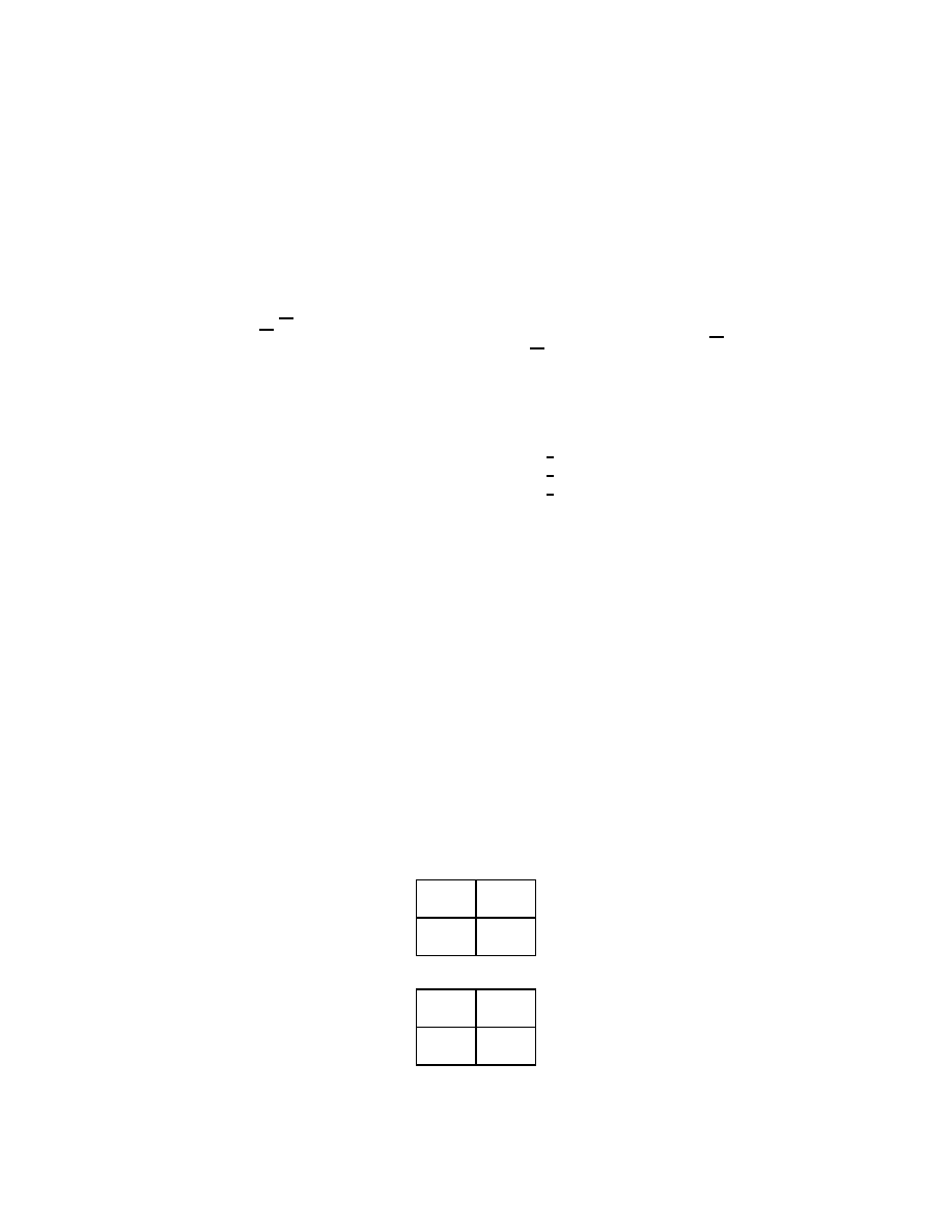
c
. In the unique equilibrium of the game
3, 3
1, 1
1, 0
0, 1
player 1 receives a payoff of 3, while in the unique equilibrium of
3, 3
1, 1
4, 0
2, 1

4
Chapter 2. Nash Equilibrium
she receives a payoff of 2. If she is prohibited from using her second action in this second
game then she obtains an equilibrium payoff of 3, however.
27.2 (BoS with imperfect information) The Bayesian game is as follows. There are two players,
say N = {1, 2}, and four states, say Ω = {(B, B), (B, S), (S, B), (S, S)}, where the state
(X, Y ) is interpreted as a situation in which player 1’s preferred composer is X and player 2’s
is Y . The set A
i
of actions of each player i is {B, S}, the set of signals that player i may
receive is {B, S}, and player i’s signal function τ
i
is defined by τ
i
(ω) = ω
i
. A belief of each
player i is a probability distribution p
i
over Ω. Player 1’s preferences are those represented by
the payoff function defined as follows. If ω
1
= B then u
1
((B, B), ω) = 2, u
1
((S, S), ω) = 1,
and u
1
((B, S), ω) = u
1
((S, B), ω) = 0; if ω
1
= S then u
1
is defined analogously. Player 2’s
preferences are defined similarly.
For any beliefs the game has Nash equilibria ((B, B), (B, B)) (i.e. each type of each
player chooses B) and ((S, S), (S, S)). If one player’s equilibrium action is independent
of his type then the other player’s is also. Thus in any other equilibrium the two types
of each player choose different actions. Whether such a profile is an equilibrium depends
on the beliefs. Let q
X
= p
2
(X, X)/[p
2
(B, X) + p
2
(S, X)] (the probability that player 2
assigns to the event that player 1 prefers X conditional on player 2 preferring X) and let
p
X
= p
1
(X, X)/[p
1
(X, B) + p
1
(X, S)] (the probability that player 1 assigns to the event
that player 2 prefers X conditional on player 1 preferring X). If, for example, p
X
≥
1
3
and
q
X
≥
1
3
for X = B, S, then ((B, S), (B, S)) is an equilibrium.
28.1 (Exchange game) In the Bayesian game there are two players, say N = {1, 2}, the set of
states is Ω = S × S, the set of actions of each player is {Exchange, Don’t exchange}, the
signal function of each player i is defined by τ
i
(s
1
, s
2
) = s
i
, and each player’s belief on Ω is
that generated by two independent copies of F . Each player’s preferences are represented
by the payoff function u
i
((X, Y ), ω) = ω
j
if X = Y = Exchange and u
i
((X, Y ), ω) = ω
i
otherwise.
Let x be the smallest possible prize and let M
i
be the highest type of player i that chooses
Exchange
. If M
i
> x then it is optimal for type x of player j to choose Exchange. Thus if
M
i
≥ M
j
and M
i
> x then it is optimal for type M
i
of player i to choose Don’t exchange,
since the expected value of the prizes of the types of player j that choose Exchange is less
than M
i
. Thus in any possible Nash equilibrium M
i
= M
j
= x: the only prizes that may
be exchanged are the smallest.
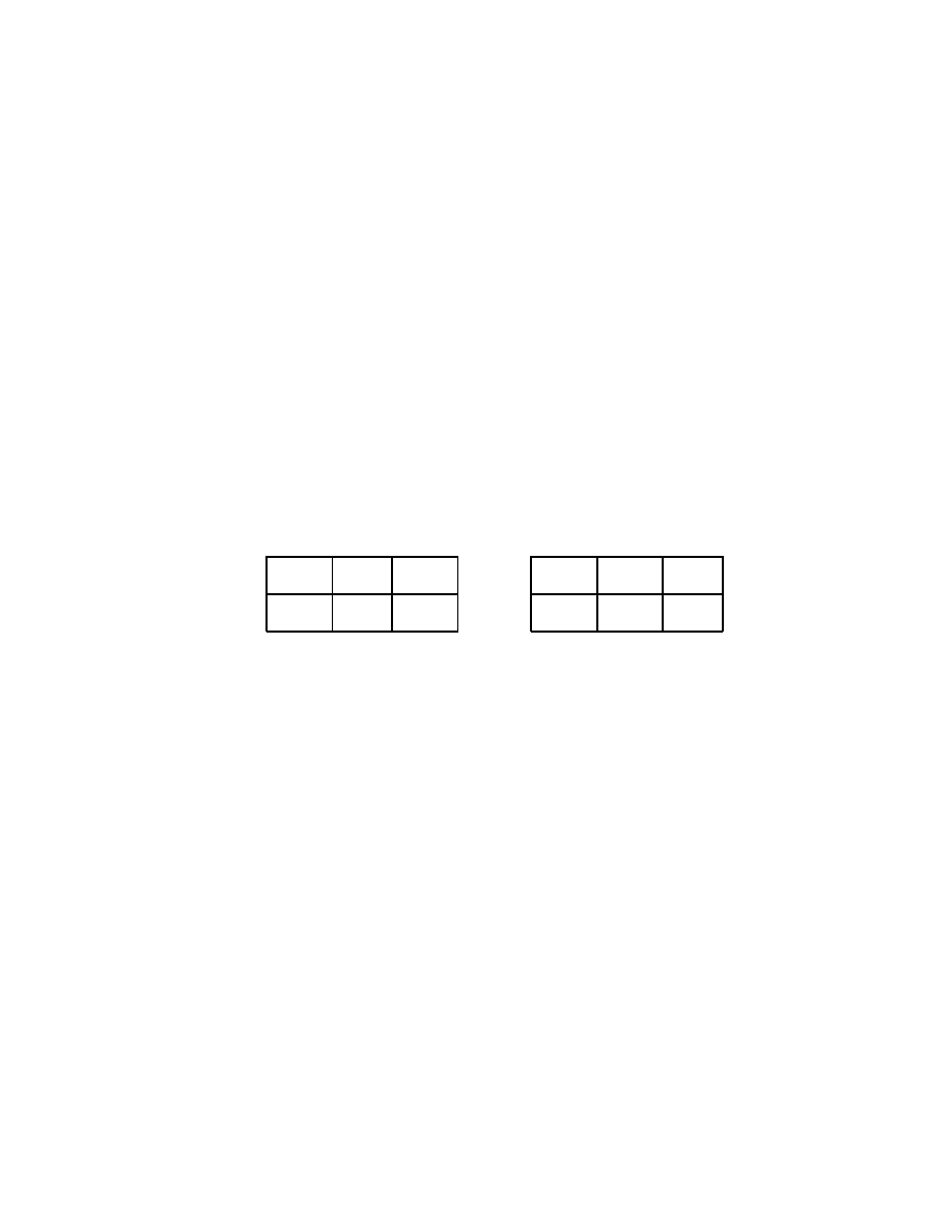
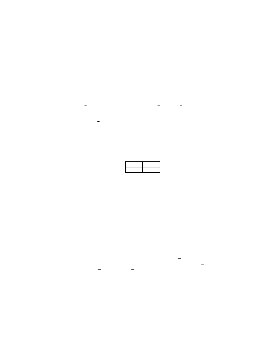
28.2 (More information may hurt) Consider the Bayesian game in which N = {1, 2}, Ω =
{ω
1
, ω
2
}, the set of actions of player 1 is {U, D}, the set of actions of player 2 is {L, M, R},
player 1’s signal function is defined by τ
1
(ω
1
) = 1 and τ
1
(ω
2
) = 2, player 2’s signal function
is defined by τ
2
(ω
1
) = τ
2
(ω
2
) = 0, the belief of each player is (
1
2
,
1
2
), and the preferences of
each player are represented by the expected value of the payoff function shown in Figure 5.1
(where 0 < <
1
2
).
This game has a unique Nash equilibrium ((D, D), L) (that is, both types of player 1
choose D and player 2 chooses L). The expected payoffs at the equilibrium are (2, 2).
In the game in which player 2, as well as player 1, is informed of the state, the unique
Nash equilibrium when the state is ω
1
is (U, R); the unique Nash equilibrium when the state
is ω
2
is (U, M ). In both cases the payoff is (1, 3), so that player 2 is worse off than he is
when he is ill-informed.
Chapter 2. Nash Equilibrium
5
L
M
R
U
1, 2
1, 0
1, 3
D
2, 2
0, 0
0, 3
State ω
1
L
M
R
U
1, 2
1, 3
1, 0
D
2, 2
0, 3
0, 0
State ω
2
Figure 5.1 The payoffs in the Bayesian game for Exercise 28.2.


3
Mixed, Correlated, and Evolutionary
Equilibrium
35.1 (Guess the average) Let k
∗
be the largest number to which any player’s strategy assigns
positive probability in a mixed strategy equilibrium and assume that player i’s strategy does
so. We now argue as follows.
• In order for player i’s strategy to be optimal his payoff from the pure strategy k
∗
must
be equal to his equilibrium payoff.
• In any equilibrium player i’s expected payoff is positive, since for any strategies of the
other players he has a pure strategy that for some realization of the other players’
strategies is at least as close to
2
3
of the average number as any other player’s number.
• In any realization of the strategies in which player i chooses k
∗
, some other player also
chooses k
∗
, since by the previous two points player i’s payoff is positive in this case,
so that no other player’s number is closer to
2
3
of the average number than k
∗
. (Note
that all the other numbers cannot be less than
2
3
of the average number.)
• In any realization of the strategies in which player i chooses k
∗
≥ 1, he can increase
his payoff by choosing k
∗
− 1, since by making this change he becomes the outright
winner rather than tying with at least one other player.
The remaining possibility is that k
∗
= 1: every player uses the pure strategy in which he
announces the number 1.
35.2 (Investment race) The set of actions of each player i is A
i
= [0, 1]. The payoff function of
player i is
u
i
(a
1
, a
2
) =
−a
i
if a
i
< a
j
1
2
− a
i
if a
i
= a
j
1 − a
i
if a
i
> a
j
,
where j ∈ {1, 2} \ {i}.
We can represent a mixed strategy of a player i in this game by a probability distribution
function F
i
on the interval [0, 1], with the interpretation that F
i
(v) is the probability that
player i chooses an action in the interval [0, v]. Define the support of F
i
to be the set of
points v for which F
i
(v + ) − F
i
(v − ) > 0 for all > 0, and define v to be an atom of F
i
if F
i
(v) > lim
↓0
F
i
(v − ). Suppose that (F
∗
1
, F
∗
2
) is a mixed strategy Nash equilibrium of
the game and let S
∗
i
be the support of F
∗
i
for i = 1, 2.
Step
. S
∗
1
= S
∗
2
.

8
Chapter 3. Mixed, Correlated, and Evolutionary Equilibrium
Proof
. If not then there is an open interval, say (v, w), to which F
∗
i
assigns positive
probability while F
∗
j
assigns zero probability (for some i, j). But then i can increase his
payoff by transferring probability to smaller values within the interval (since this does not
affect the probability that he wins or loses, but increases his payoff in both cases).
Step
. If v is an atom of F
∗
i
then it is not an atom of F
∗
j
and for some > 0 the set S
∗
j
contains no point in (v − , v).
Proof
. If v is an atom of F
∗
i
then for some > 0, no action in (v − , v] is optimal for
player j since by moving any probability mass in F
∗
i
that is in this interval to either v + δ
for some small δ > 0 (if v < 1) or 0 (if v = 1), player j increases his payoff.
Step
. If v > 0 then v is not an atom of F
∗
i
for i = 1, 2.
Proof
. If v > 0 is an atom of F
∗
i
then, using Step 2, player i can increase his payoff by
transferring the probability attached to the atom to a smaller point in the interval (v − , v).
Step
. S
∗
i
= [0, M ] for some M > 0 for i = 1, 2.
Proof
. Suppose that v /
∈ S
∗
i
and let w
∗
= inf{w: w ∈ S
∗
i
and w ≥ v} > v. By Step 1
we have w
∗
∈ S
∗
j
, and hence, given that w
∗
is not an atom of F
∗
i
by Step 3, we require
j’s payoff at w
∗
to be no less than his payoff at v. Hence w
∗
= v. By Step 2 at most one
distribution has an atom at 0, so M > 0.
Step
. S
∗
i
= [0, 1] and F
∗
i
(v) = v for v ∈ [0, 1] and i = 1, 2.
Proof
. By Steps 2 and 3 each equilibrium distribution is atomless, except possibly at
0, where at most one distribution, say F
∗
i
, has an atom. The payoff of j at v > 0 is
F
∗
i
(v) − v, where i 6= j. Thus the constancy of i’s payoff on [0, M ] and F
∗
j
(0) = 0 requires
that F
∗
j
(v) = v, which implies that M = 1. The constancy of j’s payoff then implies that
F
∗
i
(v) = v.
We conclude that the game has a unique mixed strategy equilibrium, in which each
player’s probability distribution is uniform on [0, 1].
36.1 (Guessing right) In the game each player has K actions; u
1
(k, k) = 1 for each k ∈ {1, . . . , K}
and u
1
(k, `) = 0 if k 6= `. The strategy pair ((1/K, . . . , 1/K), (1/K, . . . , 1/K)) is the unique
mixed strategy equilibrium, with an expected payoff to player 1 of 1/K. To see this, let
(p
∗
, q
∗
) be a mixed strategy equilibrium. If p
∗
k
> 0 then the optimality of the action k for
player 1 implies that q
∗
k
is maximal among all the q
∗
`
, so that in particular q
∗
k
> 0, which
implies that p
∗
k
is minimal among all the p
∗
`
, so that p
∗
k
≤ 1/K. Hence p
∗
k
= 1/K for all k;
similarly q
k
= 1/K for all k.
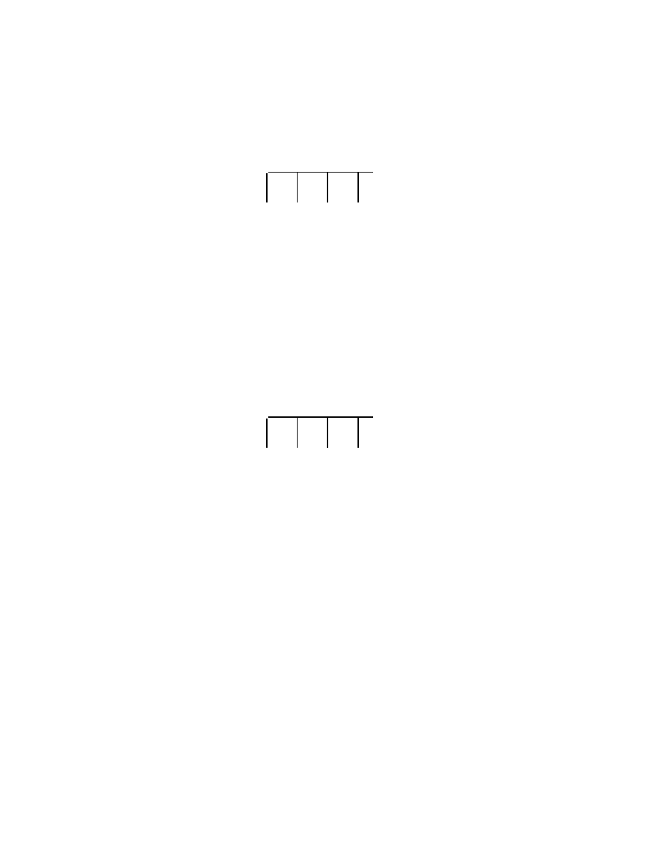
36.2 (Air strike) The payoffs of player 1 are given by the matrix
0
v
1
v
1
v
2
0
v
2
v
3
v
3
0
Let (p
∗
, q
∗
) be a mixed strategy equilibrium.
Step 1
. If p
∗
i
= 0 then q
∗
i
= 0 (otherwise q
∗
is not a best response to p
∗
); but if q
∗
i
= 0
and i ≤ 2 then p
i+1
= 0 (since player i can achieve v
i
by choosing i). Thus if for i ≤ 2
target i is not attacked then target i + 1 is not attacked either.
Chapter 3. Mixed, Correlated, and Evolutionary Equilibrium
9
Step 2
. p
∗
6= (1, 0, 0): it is not the case that only target 1 is attacked.
Step 3
. The remaining possibilities are that only targets 1 and 2 are attacked or all three
targets are attacked.
• If only targets 1 and 2 are attacked the requirement that the players be indiffer-
ent between the strategies that they use with positive probability implies that p
∗
=
(v
2
/(v
1
+v
2
), v
1
/(v
1
+v
2
), 0) and q
∗
= (v
1
/(v
1
+ v
2
),v
2
/(v
1
+ v
2
),0). Thus the expected
payoff of Army A is v
1
v
2
/(v
1
+ v
2
). Hence this is an equilibrium if v
3
≤ v
1
v
2
/(v
1
+ v
2
).
• If all three targets are attacked the indifference conditions imply that the probabilities
of attack are in the proportions v
2
v
3
: v
1
v
3
: v
1
v
2
and the probabilities of defense are
in the proportions z − 2v
2
v
3
: z − 2v
3
v
1
: z − 2v
1
v
2
where z = v
1
v
2
+ v
2
v
3
+ v
3
v
1
. For
an equilibrium we need these three proportions to be nonnegative, which is equivalent
to z − 2v
1
v
2
≥ 0, or v
3
≥ v
1
v
2
/(v
1
+ v
2
).
36.3 (Technical result on convex sets) NOTE: The following argument is simpler than the one
suggested in the first printing of the book (which is given afterwards).
Consider the strictly competitive game in which the set of actions of player 1 is X, that
of player 2 is Y , the payoff function of player 1 is u
1
(x, y) = −x · y, and the payoff function
of player 2 is u
2
(x, y) = x · y. By Proposition 20.3 this game has a Nash equilibrium, say
(x
∗
, y
∗
); by the definition of an equilibrium we have x
∗
· y ≤ x
∗
· y
∗
≤ x · y
∗
for all x ∈ X
and y ∈ Y .
The argument suggested in the first printing of the book (which is elementary, not relying
on the result that an equilibrium exists, but more difficult than the argument given in the
previous paragraph) is the following.
Let G(n) be the strictly competitive game in which each player has n actions and the
payoff function of player 1 is given by u
1
(i, j) = x
i
· y
j
. Let v(n) be the value of G(n) and let
α
n
be a mixed strategy equilibrium. Then U
1
(α
1
, α
n
2
) ≤ v(n) ≤ U
1
(α
n
1
, α
2
) for every mixed
strategy α
1
of player 1 and every mixed strategy α
2
of player 2 (by Proposition 22.2). Let
x
∗n
=
P
n
i=1
α
n
1
(i)x
i
and y
∗n
=
P
n
j=1
α
n
2
(j)y
j
. Then x
i
· y
∗n
≤ v(n) = x
∗n
y
∗n
≤ x
∗n
· y
j
for
all i and j. Letting n → ∞ through a subsequence for which x
∗n
and y
∗n
converge, say to
x
∗
and y
∗
, we obtain the result.
42.1 (Examples of Harsanyi’s purification)
1
a
. The pure equilibria are trivially approachable. Now consider the strictly mixed equi-
librium. The payoffs in the Bayesian game G(γ) are as follows:
a
2
b
2
a
1
2 + γδ
1
, 1 + γδ
2
γδ
1
, 0
a
2
0, γδ
2
1, 2
For i = 1, 2 let p
i
be the probability that player i’s type is one for which he chooses a
i
in
some Nash equilibrium of G(γ). Then it is optimal for player 1 to choose a
1
if
(2 + γδ
1
)p
2
≥ (1 − γδ
1
)(1 − p
2
),
1
Correction to first printing of book
: The
1
(x, b
2
) near the end of line −4 should be
2
(x, b
2
).
10
Chapter 3. Mixed, Correlated, and Evolutionary Equilibrium
or δ
1
≥ (1 − 3p
2
)/γ. Now, the probability that δ
1
is at least (1 − 3p
2
)/γ is
1
2
(1 − (1 − 3p
2
)/γ)
if −1 ≤ (1 − 3p
2
)/γ ≤ 1, or
1
3
(1 − γ) ≤ p
2
≤
1
3
(1 + γ). This if p
2
lies in this range we have
p
1
=
1
2
(1 − (1 − 3p
2
)/γ). By a symmetric argument we have p
2
=
1
2
(1 − (2 − 3p
1
)/γ) if
1
3
(2 − γ) ≤ p
1
≤
1
3
(2 + γ). Solving for p
1
and p
2
we find that p
1
= (2 + γ)/(3 + 2γ) and
p
2
= (1 + γ)/(3 + 2γ) satisfies these conditions. Since (p
1
, p
2
) → (
2
3
,
1
3
) as γ → 0 the mixed
strategy equilibrium is approachable.
b
. The payoffs in the Bayesian game G(γ) are as follows:
a
2
b
2
a
1
1 + γδ
1
, 1 + γδ
2
γδ
1
, 0
a
2
0, γδ
2
0, 0
For i = 1, 2 let p
i
be the probability that player i’s type is one for which he chooses a
i
in some
Nash equilibrium of G(γ). Whenever δ
j
> 0, which occurs with probability
1
2
, the action a
j
dominates b
j
; thus we have p
j
≥
1
2
. Now, player i’s payoff to a
i
is p
j
(1 + γδ
i
) + (1 − p
j
)γδ
i
=
p
j
+ γδ
i
, which, given p
j
≥
1
2
, is positive for all values of δ
i
if γ <
1
2
. Thus if γ <
1
2
all
types of player i choose a
i
. Hence if γ <
1
2
the Bayesian game G(γ) has a unique Nash
equilibrium, in which every type of each player i uses the pure strategy a
i
. Thus only the
pure strategy equilibrium (a
1
, a
2
) of the original game is approachable.
c
. In any Nash equilibrium of the Bayesian game G(γ) player i chooses a
i
whenever
δ
i
> 0 and b
i
whenever δ
i
< 0; since δ
i
is positive with probability
1
2
and negative with
probability
1
2
the result follows.
48.1 (Example of correlated equilibrium)
a
. The pure strategy equilibria are (B, L, A), (T, R, A), (B, L, C), and (T, R, C).
b
. A correlated equilibrium with the outcome described is given by: Ω = {x, y}, π(x) =
π(y) =
1
2
; P
1
= P
2
= {{x}, {y}}, P
3
= Ω; σ
1
({x}) = T , σ
1
({y}) = B; σ
2
({x}) = L,
σ
2
({y}) = R; σ
3
(Ω) = B. Note that player 3 knows that (T, L) and (B, R) will occur with
equal probabilities, so that if she deviates to A or C she obtains
3
2
< 2.
c
. If player 3 were to have the same information as players 1 and 2 then the outcome
would be one of those predicted by the notion of Nash equilibrium, in all of which she
obtains a payoff of zero.
51.1 (Existence of ESS in 2 × 2 game) Let the game be as follows:
C
D
C
w, w
x, y
D
y, x
z, z
If w > y then (C, C) is a strict equilibrium, so that C is an ESS. If z > x then (D, D)
is a strict equilibrium, so that D is an ESS. If w < y and z < x then the game has
a symmetric mixed strategy equilibrium (m
∗
, m
∗
) in which m
∗
attaches the probability
p
∗
= (z − x)/(w − y + z − x) to C. To verify that m
∗
is an ESS, we need to show that
u(m, m) < u(m
∗
, m) for any mixed strategy m 6= m
∗
. Let p be the probability that m
attaches to C. Then
u(m, m) − u(m
∗
, m) = (p − p
∗
)[pw + (1 − p)x] − (p − p
∗
)[py + (1 − p)z]
= (p − p
∗
)[p(w − y + z − x) + x − z]
= (p − p
∗
)
2
(w − y + z − x)
< 0.

4
Rationalizability and Iterated
Elimination of Dominated Actions
56.3 (Example of rationalizable actions) The actions of player 1 that are rationalizable are a
1
,
a
2
, and a
3
; those of player 2 are b
1
, b
2
, and b
3
. The actions a
2
and b
2
are rationalizable
since (a
2
, b
2
) is a Nash equilibrium. Since a
1
is a best response to b
3
, b
3
is a best response
to a
3
, a
3
is a best response to b
1
, and b
1
is a best response to a
1
the actions a
1
, a
3
, b
1
,
and b
3
are rationalizable. The action b
4
is not rationalizable since if the probability that
player 2’s belief assigns to a
4
exceeds
1
2
then b
3
yields a payoff higher than does b
4
, while
if this probability is at most
1
2
then b
2
yields a payoff higher than does b
4
. The action a
4
is not rationalizable since without b
4
in the support of player 1’s belief, a
4
is dominated by
a
2
.
Comment
That b
4
is not rationalizable also follows from Lemma 60.1, since b
4
is strictly
dominated by the mixed strategy that assigns the probability
1
3
to b
1
, b
2
, and b
3
.
56.4 (Cournot duopoly) Player i’s best response function is B
i
(a
j
) = (1 − a
j
)/2; hence the only
Nash equilibrium is (
1
3
,
1
3
).
Since the game is symmetric, the set of rationalizable actions is the same for both players;
denote it by Z. Let m = inf Z and M = sup Z. Any best response of player i to a belief of
player j whose support is a subset of Z maximizes E[a
i
(1 − a
i
− a
j
)] = a
i
(1 − a
i
− E[a
j
]),
and thus is equal to B
i
(E[a
j
]) ∈ [B
j
(M ), B
j
(m)] = [(1 − M )/2, (1 − m)/2]. Hence (using
Definition 55.1), we need (1 − M )/2 ≤ m and M ≤ (1 − m)/2, so that M = m =
1
3
:
1
3
is
the only rationalizable action of each player.
56.5 (Guess the average) Since the game is symmetric, the set of rationalizable actions is the
same, say Z, for all players. Let k
∗
be the largest number in Z. By the argument in the
solution to Exercise 35.1 the action k
∗
is a best response to a belief whose support is a
subset of Z only if k
∗
= 1. The result follows from Definition 55.1.
57.1 (Modified rationalizability in location game) The best response function of each player i is
B
i
(a
j
) = {a
j
}. Hence (a
1
, a
2
) is a Nash equilibrium if and only if a
1
= a
2
for i = 1, 2. Thus
any x ∈ [0, 1] is rationalizable.
Fix i ∈ {1, 2} and define a pair (a
i
, d) ∈ A
i
× [0, 1] (where d is the information about
the distance to a
j
) to be rationalizable if for j = 1, 2 there is a subset Z
j
of A
j
such that
a
i
∈ Z
i
and every action a
j
∈ Z
j
is a best response to a belief of player j whose support is
a subset of Z
k
∩ {a
j
+ d, a
j
− d} (where k 6= j).
12
Chapter 4. Rationalizability and Iterated Elimination of Dominated Actions
In order for (a
i
, d) to be rationalizable the action a
i
must be a best response to a belief
that is a subset of {a
i
+ d, a
i
− d}. This belief must assign positive probability to both
points in the set (otherwise the best response is to locate at one of the points). Thus Z
j
must contain both a
i
+ d and a
i
− d, and hence each of these must be best responses for
player j to beliefs with supports {a
i
+ 2d, a
i
} and {a
i
, a
i
− 2d}. Continuing the argument
we conclude that Z
j
must contain all points of the form a
i
+ md for every integer m, which
is not possible if d > 0 since A
i
= [0, 1]. Hence (a
i
, d) is rationalizable only if d = 0; it is
easy to see that (a
i
, 0) is in fact rationalizable for any a
i
∈ A
i
.
63.1 (Iterated elimination in location game) Only one round of elimination is needed: every
action other than
1
2
is weakly dominated by the action
1
2
. (In fact
1
2
is the only action that
survives iterated elimination of strictly dominated actions: on the first round Out is strictly
dominated by
1
2
, and in every subsequent round each of the remaining most extreme actions
is strictly dominated by
1
2
.)
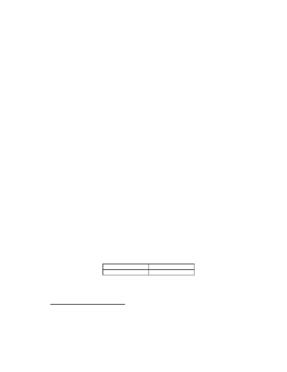
63.2 (Dominance solvability) Consider the game in Figure 12.1. This game is dominance solvable,
the only surviving outcome being (T, L). However, if B is deleted then neither of the
remaining actions of player 2 is dominated, so that both (T, L) and (T, R) survive iterated
elimination of dominated actions.
L
R
T
1, 0
0, 0
B
0, 1
0, 0
Figure 12.1 The game for the solution to Exercise 63.2.
64.1 (Announcing numbers) At the first round every action a
i
≤ 50 of each player i is weakly
dominated by a
i
+1. No other action is weakly dominated, since 100 is a strict best response
to 0 and every other action a
i
≥ 51 is a best response to a
i
+ 1. At every subsequent round
up to 50 one action is eliminated for each player: at the second round this action is 100, at
the third round it is 99, and so on. After round 50 the single action pair (51, 51) remains,
with payoffs of (50, 50).
64.2 (Non-weakly dominated action as best response) From the result in Exercise 36.3, for any
there exist p() ∈ P () and u() ∈ U such that
p() · u ≤ p() · u() ≤ p · u() for all p ∈ P (), u ∈ U.
Choose any sequence
n
→ 0 such that u(
n
) converges to some u. Since u
∗
= 0 ∈ U we
have 0 ≤ p(
n
) · u(
n
) ≤ p · u(
n
) for all n and all p ∈ P (0) and hence p · u ≥ 0 for all
p ∈ P (0). It follows that u ≥ 0 and hence u = u
∗
, since u
∗
corresponds to a mixed strategy
that is not weakly dominated.
Finally, p(
n
) · u ≤ p(
n
) · u(
n
) for all u ∈ U , so that u
∗
is in the closure of the set
B of members of U for which there is a supporting hyperplane whose normal has positive
components. Since U is determined by a finite set, the set B is closed. Thus there exists a
strictly positive vector p
∗
with p
∗
· u
∗
≥ p
∗
· u for all u ∈ U .
Comment
This exercise is quite difficult.

5
Knowledge and Equilibrium
69.1 (Example of information function) No, P may not be partitional. For example, it is not
if the answers to the three questions at ω
1
are (Yes, No, No) and the answers at ω
2
are
(Yes, No, Yes), since ω
2
∈ P (ω
1
) but P (ω
1
) 6= P (ω
2
).
69.2 (Remembering numbers) The set of states Ω is the set of integers and P (ω) = {ω−1, ω, ω+1}
for each ω ∈ Ω. The function P is not partitional: 1 ∈ P (0), for example, but P (1) 6= P (0).
71.1 (Information functions and knowledge functions)
a
. P
0
(ω) is the intersection of all events E for which ω ∈ K(E) and thus is the intersection
of all E for which P (ω) ⊆ E, and this intersection is P (ω) itself.
b
. K
0
(E) consists of all ω for which P (ω) ⊆ E, where P (ω) is equal to the intersection
of the events F that satisfy ω ∈ K(F ). By K1, P (ω) ⊆ Ω.
Now, if ω ∈ K(E) then P (ω) ⊆ E and therefore ω ∈ K
0
(E). On the other hand if
ω ∈ K
0
(E) then P (ω) ⊆ E, or E ⊇ ∩{F ⊆ Ω: K(F ) 3 ω}. Thus by K2 we have K(E) ⊇
K(∩{F ⊆ Ω: K(F ) 3 ω}), which by K3 is equal to ∩{K(F ): F ⊆ Ω and K(F ) 3 ω}), so
that ω ∈ K(E). Hence K(E) = K
0
(E).
71.2 (Decisions and information) Let a be the best act under P and let a
0
be the best act under
P
0
. Then a
0
is feasible under P and the expected payoff from a
0
is
X
k
π(P
k
)E
π
k
u(a
0
(P
0
(P
k
)), ω),
where {P
1
, . . . , P
K
} is the partition induced by P , π
k
is π conditional of P
k
, P
0
(P
k
) is the
member of the partition induced by P
0
that contains P
k
, and we write a
0
(P
0
(P
k
)) for the
action a
0
(ω) for any ω ∈ P
0
(P
k
). The result follows from the fact that for each value of k
we have
E
π
k
u(a(P
k
), ω) ≥ E
π
k
u(a
0
(P
0
(P
k
)), ω).
76.1 (Common knowledge and different beliefs) Let Ω = {ω
1
, ω
2
}, suppose that the partition
induced by individual 1’s information function is {{ω
1
, ω
2
}} and that induced by individ-
ual 2’s is {{ω
1
}, {ω
2
}}, assume that each individual’s prior is (
1
2
,
1
2
), and let E be the
event {ω
1
}. The event “individual 1 and individual 2 assign different probabilities to E” is
{ω ∈ Ω: ρ(E|P
1
(ω)) 6= ρ(E|P
2
(ω))} = {ω
1
, ω
2
}, which is clearly self-evident, and hence is
common knowledge in either state.

14
Chapter 5. Knowledge and Equilibrium
The proof of the second part follows the lines of the proof of Proposition 75.1. The
event “the probability assigned by individual 1 to X exceeds that assigned by individual 2”
is E = {ω ∈ Ω: ρ(X|P
1
(ω)) > ρ(X|P
2
(ω))}. If this event is common knowledge in the
state ω then there is a self-evident event F 3 ω that is a subset of E and is a union of
members of the information partitions of both individuals. Now, for all ω ∈ F we have
ρ(X|P
1
(ω)) > ρ(X|P
2
(ω)), so that
X
ω∈F
ρ(ω)ρ(X|P
1
(ω)) >
X
ω∈F
ρ(ω)ρ(X|P
2
(ω)).
But since F is a union of members of each individual’s information partition both sides of
this inequality are equal to ρ(X ∩ F ), a contradiction. Hence E is not common knowledge.
76.2 (Common knowledge and beliefs about lotteries) Denote the value of the lottery in state ω
by L(ω). Define the event E by
E = {ω ∈ Ω: e
1
(L|P
1
(ω)) > η and e
2
(L|P
2
(ω)) < η},
where e
i
(L|P
i
(ω)) =
P
ω
0
∈P
i
(ω)
ρ(ω
0
|P
i
(ω))L(ω
0
) is individual i’s belief about the expec-
tation of the lottery. If this event is common knowledge in some state then there is a
self-evident event F ⊆ E. Hence in every member of individual 1’s information partition
that is a subset of F the expected value of L exceeds η. Therefore e
1
(L|F ) > η: the expected
value of the lottery given F is at least η. Analogously, the expected value of L given F is
less than η, a contradiction.
Comment
If this result were not true then a mutually profitable trade between the
individuals could be made. The existence of such a pair of beliefs is necessary for the
existence of a rational expectations equilibrium in which the individuals are aware of the
existing price, take it into consideration, and trade the lottery L even though they are
risk-neutral.
Example for non-partitional information functions
: Let Ω = {ω
1
, ω
2
, ω
3
}, ρ(ω
i
) =
1
3
for
all ω ∈ Ω, P
1
(ω) = {ω
1
, ω
2
, ω
3
} for all ω ∈ Ω, P
2
(ω
1
) = {ω
1
, ω
2
}, P
2
(ω
2
) = {ω
2
}, and
P
2
(ω
3
) = {ω
2
, ω
3
} (so that P
2
is not partitional). Let L(ω
2
) = 1 and L(ω
1
) = L(ω
3
) = 0
and let η = 0.4. Then for all ω ∈ Ω it is common knowledge that player 1 believes that the
expectation of L is
1
3
and that player 2 believes that the expectation of L is either 0.5 or 1.
81.1 (Knowledge and correlated equilibrium) By the rationality of player i in every state, for
every ω ∈ Ω the action a
i
(ω) is a best response to player i’s belief, which by assumption is
derived from the common prior ρ and P
i
(ω). Thus for all ω ∈ Ω and all i ∈ N the action
a
i
(ω) is a best response to the conditional probability derived from ρ, as required by the
definition of correlated equilibrium.

6
Extensive Games with Perfect
Information
94.2 (Extensive games with 2 × 2 strategic forms) First suppose that (a
0
1
, a
0
2
) ∼
i
(a
0
1
, a
00
2
) for
i = 1, 2. Then G is the strategic form of the extensive game with perfect information in
Figure 15.1 (with appropriate assumptions on the players’ preferences). The other case is
similar.
Now assume that G is the strategic form of an extensive game Γ with perfect information.
Since each player has only two strategies in Γ, for each player there is a single history after
which he makes a (non-degenerate) move. Suppose that player 1 moves first. Then player 2
can move after only one of player 1’s actions, say a
00
1
. In this case player 1’s action a
0
1
leads
to a terminal history, so that the combination of a
0
1
and either of the strategies of player 2
leads to the same terminal history; thus (a
0
1
, a
0
2
) ∼
i
(a
0
1
, a
00
2
) for i = 1, 2.
b
1
a
00
1
a
0
1
@
@
@
r
r
@
@
@
r
r
2
a
00
2
a
0
2
Figure 15.1 The game for the solution to Exercise 94.2.
98.1 (SPE of Stackelberg game) Consider the game in Figure 15.2. In this game (L, AD) is a
subgame perfect equilibrium, with a payoff of (1, 0), while the solution of the maximization
problem is (R, C), with a payoff of (2, 1).
b
1
L
R
HH
H
H
r
@
@
r
1, 0
1, 0
r
2
A
B
r
@
@
r
2, 1
0, 1
r
2
D
C
Figure 15.2 The extensive game in the solution of Exercise 98.1.
16
Chapter 6. Extensive Games with Perfect Information
99.1 (Necessity of finite horizon for one deviation property) In the (one-player) game in Fig-
ure 16.1 the strategy in which the player chooses d after every history satisfies the condition
in Lemma 98.2 but is not a subgame perfect equilibrium.
b
d
d
d
d
a
a
a
r
r
r
r
r
r
r
. . .
0
0
0
0
1
1
1
1
Figure 16.1 The beginning of a one-player infinite horizon game for which the one deviation
property does not hold. The payoff to the (single) infinite history is 1.
100.1 (Necessity of finiteness for Kuhn’s theorem) Consider the one-player game in which the
player chooses a number in the interval [0, 1), and prefers larger numbers to smaller ones.
That is, consider the game h{1}, {∅} ∪ [0, 1), P, {%
1
}i in which P (∅) = 1 and x
1
y if and
only if x > y. This game has a finite horizon (the length of the longest history is 1) but has
no subgame perfect equilibrium (since [0, 1) has no maximal element).
In the infinite-horizon one-player game the beginning of which is shown in Figure 16.2
the single player chooses between two actions after every history. After any history of length
k the player can choose to stop and obtain a payoff of k + 1 or to continue; the payoff if she
continues for ever is 0. The game has no subgame perfect equilibrium.
b
r
r
r
r
r
r
r
. . .
1
2
3
4
1
1
1
1
Figure 16.2 The beginning of a one-player game with no subgame perfect equilibrium.
The payoff to the (single) infinite history is 0.
100.2 (SPE of games satisfying no indifference condition) The hypothesis is true for all subgames
of length one. Assume the hypothesis for all subgames with length at most k. Consider
a subgame Γ(h) with `(Γ(h)) = k + 1 and P (h) = i. For all actions a of player i such
that (h, a) ∈ H define R(h, a) to be the outcome of some subgame perfect equilibrium of
the subgame Γ(h, a). By hypothesis all subgame perfect equilibria outcomes of Γ(h, a) are
preference equivalent; in a subgame perfect equilibrium of Γ(h) player i takes an action that
maximizes %
i
over {R(h, a): a ∈ A(h)}. Therefore player i is indifferent between any two
subgame perfect equilibrium outcomes of Γ(h); by the no indifference condition all players
are indifferent among all subgame perfect equilibrium outcomes of Γ(h).
We now show that the equilibria are interchangeable. For any subgame perfect equi-
librium we can attach to every subgame the outcome according to the subgame perfect
equilibrium if that subgame is reached. By the first part of the exercise the outcomes that
we attach (or at least the rankings of these outcomes in the players’ preferences) are in-
dependent of the subgame perfect equilibrium that we select. Thus by the one deviation
property (Lemma 98.2), any strategy profile s
00
in which for each player i the strategy s
00
i
is
equal to either s
i
or s
0
i
is a subgame perfect equilibrium.

Chapter 6. Extensive Games with Perfect Information
17
101.1 (SPE and unreached subgames) This follows directly from the definition of a subgame per-
fect equilibrium.
101.2 (SPE and unchosen actions) The result follows directly from the definition of a subgame
perfect equilibrium.
101.3 (Armies) We model the situation as an extensive game in which at each history at which
player i occupies the island and player j has at least two battalions left, player j has two
choices: conquer the island or terminate the game. The first player to move is player 1. (We
do not specify the game formally.)
We show that in every subgame in which army i is left with y
i
battalions (i = 1, 2) and
army j occupies the island, army i attacks if and only if either y
i
> y
j
, or y
i
= y
j
and y
i
is
even.
The proof is by induction on min{y
1
, y
2
}. The claim is clearly correct if min{y
1
, y
2
} ≤ 1.
Now assume that we have proved the claim whenever min{y
1
, y
2
} ≤ m for some m ≥ 1.
Suppose that min{y
1
, y
2
} = m + 1. There are two cases.
• either y
i
> y
j
, or y
i
= y
j
and y
i
is even: If army i attacks then it occupies the island
and is left with y
i
− 1 battalions. By the induction hypothesis army j does not launch
a counterattack in any subgame perfect equilibrium, so that the attack is worthwhile.
• either y
i
< y
j
, or y
i
= y
j
and y
i
is odd: If army i attacks then it occupies the
island and is left with y
i
− 1 battalions; army j is left with y
j
battalions. Since either
y
i
− 1 < y
j
− 1 or y
i
− 1 = y
j
− 1 and is even, it follows from the inductive hypothesis
that in all subgame perfect equilibria there is a counterattack. Thus army i is better
off not attacking.
Thus the claim is correct whenever min{y
1
, y
2
} ≤ m+1, completing the inductive argument.
102.1 (ODP and Kuhn’s theorem with chance moves)
One deviation property
: The argument is the same as in the proof of Lemma 98.2.
Kuhn’s theorem
: The argument is the same as in the proof of Proposition 99.2 with the
following addition. If P (h
∗
) = c then R(h
∗
) is the lottery in which R(h
∗
, a) occurs with
probability f
c
(a|h) for each a ∈ A(h
∗
).
103.1 (Three players sharing pie) The game is given by
• N = {1, 2, 3}
• H = {∅} ∪ X ∪ {(x, y): x ∈ X and y ∈ {yes, no} × {yes, no}} where X = {x ∈
R
3
+
:
P
3
i=1
x
i
= 1}
• P (∅) = 1 and P (x) = {2, 3} if x ∈ X
• for each i ∈ N we have (x, (yes, yes))
i
(z, (yes, yes)) if and only if x
i
> z
i
; if (A, B) 6=
(yes, yes) then (x, (yes, yes))
i
(z, (A, B)) if x
i
> 0 and (x, (yes, yes)) ∼
i
(z, (A, B))
if x
i
= 0; if (A, B) 6= (yes, yes) and (C, D) 6= (yes, yes) then (x, (C, D)) ∼
i
(z, (A, B))
for all x ∈ X and z ∈ X.

18
Chapter 6. Extensive Games with Perfect Information
In each subgame that follows a proposal x of player 1 there are two types of Nash
equilibria. In one equilibrium, which we refer to as Y (x), players 2 and 3 both accept x. In
all the remaining equilibria the proposal x is not implemented; we refer to the set of these
equilibria as N (x). If both x
2
> 0 and x
3
> 0 then N (x) consists of the single equilibrium
in which players 2 and 3 both reject x. If x
i
= 0 for either i = 2 or i = 3, or both, then
N (x) contains in addition equilibria in which a player who is offered 0 rejects the proposal
and the other player accepts the proposal.
Consequently the equilibria of the entire game are the following.
• For any division x, player 1 proposes x. In the subgame that follows the proposal x
of player 1, the equilibrium is Y (x). In the subgame that follows any proposal y of
player 1 in which y
1
> x
1
, the equilibrium is in N (y). In the subgame that follows any
proposal y of player 1 in which y
1
< x
1
, the equilibrium is either Y (y) or is in N (y).
• For any division x, player 1 proposes x. In the subgame that follows any proposal y of
player 1 in which y
1
> 0, the equilibrium is in N (y). In the subgame that follows any
proposal y of player 1 in which y
1
= 0, the equilibrium is either Y (y) or is in N (y).
103.2 (Naming numbers) The game is given by
• N = {1, 2}
• H = {∅} ∪ {Stop, Continue} ∪ {(Continue, y): y ∈ Z × Z} where Z is the set of
nonnegative integers
• P (∅) = 1 and P (Continue) = {1, 2}
• the preference relation of each player is determined by the payoffs given in the question.
In the subgame that follows the history Continue there is a unique subgame perfect
equilibrium, in which both players choose 0. Thus the game has a unique subgame perfect
equilibrium, in which player 1 chooses Stop and, if she chooses Continue, both players choose
0.
Note that if the set of actions of each player after player 1 chooses Continue were bounded
by some number M then there would be an additional subgame perfect equilibrium in which
player 1 chooses Continue and each player names M , with the payoff profile (M
2
, M
2
).
103.3 (ODP and Kuhn’s theorem with simultaneous moves)
One deviation property
: The argument is the same as in the proof of Lemma 98.2.
Kuhn’s theorem
: Consider the following game (which captures the same situation as
Matching Pennies (Figure 17.3)):
• N = {1, 2}
• H = {∅} ∪ {x ∈ {Head, Tail} × {Head, Tail}
• P (∅) = {1, 2}
• (Head, Head) ∼
1
(Tail, Tail)
1
(Head, Tail) ∼
1
(Tail, Head) and (Head, Tail) ∼
2
(Tail, Head)
2
(Head, Head) ∼
2
(Tail, Tail).
This game has no subgame perfect equilibrium.

Chapter 6. Extensive Games with Perfect Information
19
108.1 (-equilibrium of centipede game) Consider the following pair of strategies. In every period
before k both players choose C; in every subsequent period both players choose S. The
outcome is that the game stops in period k. We claim that if T ≥ 1/ then this strategy
pair is a Nash equilibrium. For concreteness assume that k is even, so that it is player 2’s
turn to act in period k. Up to period k − 2 both players are worse off if they choose S rather
than C. In period k − 1 player 1 gains 1/T ≤ by choosing S. In period k player 2 is better
off choosing S (given the strategy of player 1), and in subsequent periods the action that
each player chooses has no effect on the outcome. Thus the strategy pair is an -equilibrium
of the game.
114.1 (Variant of the game Burning money) Player 1 has eight strategies, each of which can be
written as (x, y, z), where x ∈ {0, D} and y and z are each members of {B, S}, y being the
action that player 1 plans in BoS if player 2 chooses 0 and z being the action that player 1
plans in BoS if player 2 chooses D. Player 2 has sixteen strategies, each of which can be
written as a pair of members of the set {(0, B), (0, S), (D, B), (D, S)}, the first member of
the pair being player 2’s actions if player 1 chooses 0 and the second member of the pair
being player 2’s actions if player 1 chooses D.
Weakly dominated actions can be iteratively eliminated as follows.
1. (D, S, S) is weakly dominated for player 1 by (0, B, B)
Every strategy (a, b) of player 2 in which either a or b is (D, B) is weakly dominated
by the strategy that differs only in that (D, B) is replaced by (0, S).
2. Every strategy (x, y, B) of player 1 is weakly dominated by (x, y, S) (since there is no
remaining strategy of player 2 in which he chooses (D, B)).
3. Every strategy (a, b) of player 2 in which b is either (0, B) or (0, S) is weakly dominated
by the strategy that differs only in that b is replaced by (D, S) (since in every remaining
strategy player 1 chooses S after player 2 chooses D).
The game that remains is shown in Figure 20.1.
4. (D, B, S) is weakly dominated for player 1 by (0, B, S)
(0, B), (D, S)) is weakly dominated for player 2 by ((D, S), (D, S))
5. (0, B, S) is weakly dominated for player 1 by (0, S, S)
6. ((D, S), (D, S)) is strictly dominated for player 2 by ((0, S), (D, S))
The only remaining strategy pair is ((0, S, S), ((0, S), (D, S))), yielding the outcome (1, 3)
(the one that player 2 most prefers).
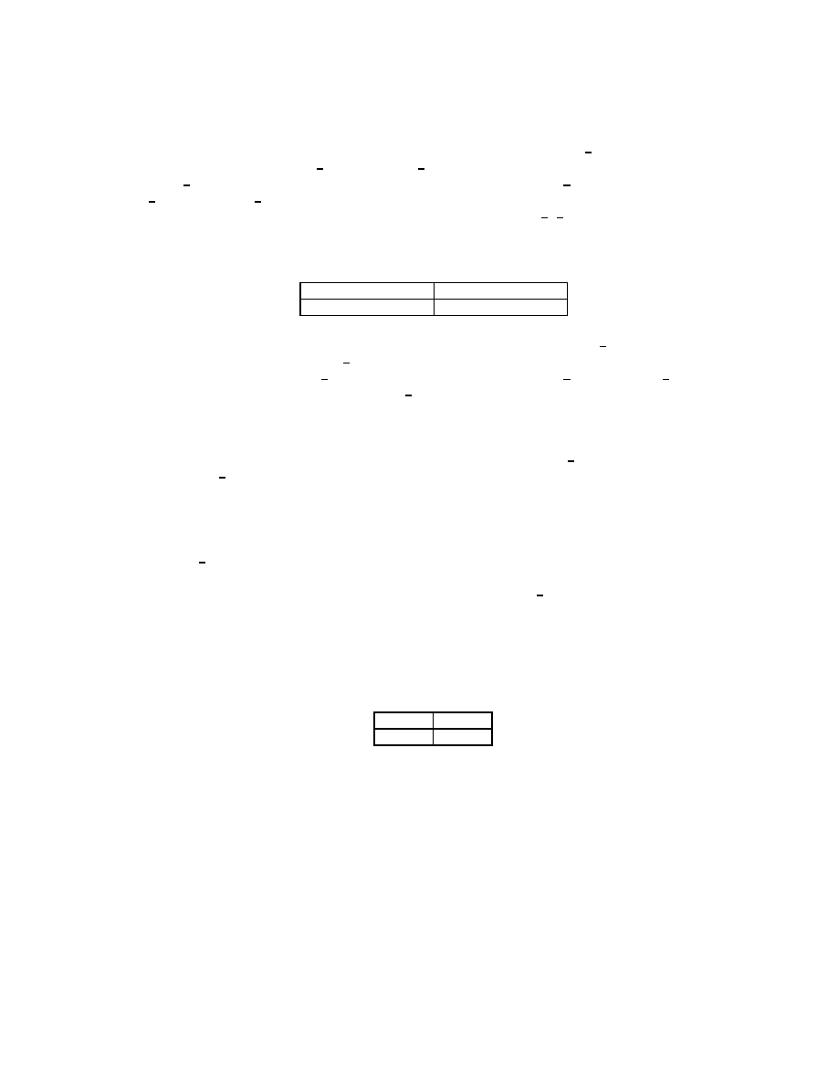
114.2 (Variant of the game Burning money) The strategic form of the game is given in Figure 20.2.
Weakly dominated actions can be eliminated iteratively as follows.
1. DB is weakly dominated for player 1 by 0B
2. AB is weakly dominated for player 2 by AA
BB is weakly dominated for player 2 by BA
3. 0B is strictly dominated for player 1 by DA
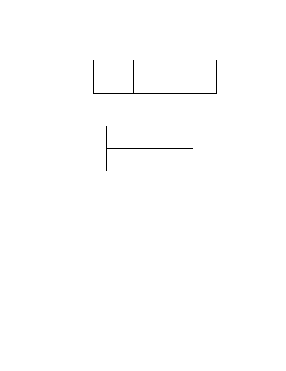
20
Chapter 6. Extensive Games with Perfect Information
(0, B), (D, S))
((0, S), (D, S))
((D, S), (D, S))
(0, B, S)
3, 1
0, 0
1, 2
(0, S, S)
0, 0
1, 3
1, 2
(D, B, S)
0, 2
0, 2
0, 2
Figure 20.1 The game in Exercise 114.1 after three rounds of elimination of weakly dom-
inated strategies.
AA
AB
BA
BB
0A
2, 2
2, 2
0, 0
0, 0
0B
0, 0
0, 0
1, 1
1, 1
DA
1, 2
−1, 0
1, 2
−1, 0
DB
−1, 0
0, 1
−1, 0
0, 1
Figure 20.2 The game for Exercise 114.2.
4. BA is weakly dominated for player 2 by AA
5. DA is strictly dominated for player 1 by 0A
The single strategy pair that remains is (0A, AA).

7
A Model of Bargaining
123.1 (One deviation property for bargaining game) The proof is similar to that of Lemma 98.2;
the sole difference is that the existence of a profitable deviant strategy that differs from s
∗
after a finite number of histories follows from the fact that the single infinite history is the
worst possible history in the game.
125.2 (Constant cost of bargaining)
a
. It is straightforward to check that the strategy pair is a subgame perfect equilibrium.
Let M
i
(G
i
) and m
i
(G
i
) be as in the proof of Proposition 122.1 for i = 1, 2. By the argument
for (124.1) with the roles of the players reversed we have M
2
(G
2
) ≤ 1 − m
1
(G
1
) + c
1
, or
m
1
(G
1
) ≤ 1 − M
2
(G
2
) + c
1
. Now suppose that M
2
(G
2
) ≥ c
2
. Then by the argument
for (123.2) with the roles of the players reversed we have m
1
(G
1
) ≥ 1 − M
2
(G
2
) + c
2
, a
contradiction (since c
1
< c
2
). Thus M
2
(G
2
) < c
2
. But now the argument for (123.2) implies
that m
1
(G
1
) ≥ 1, so that m
1
(G
1
) = 1 and hence M
1
(G
1
) = 1. Since (124.1) implies that
M
2
(G
2
) ≤ 1 − m
1
(G
1
) + c
1
we have M
2
(G
2
) ≤ c
1
; by (123.2) we have m
2
(G
2
) ≥ c
1
, so
that M
2
(G
2
) = m
2
(G
2
) = c
1
. The remainder of the argument follows as in the proof of
Proposition 122.1.
b
. First note that for any pair (x
∗
, y
∗
) of proposals in which x
∗
1
≥ c and y
∗
1
= x
∗
1
− c the
pair of strategies described in Proposition 122.1 is a subgame perfect equilibrium. Refer to
this equilibrium as E(x
∗
).
Now suppose that c <
1
3
. An example of an equilibrium in which agreement is reached
with delay is the following. Player 1 begins by proposing (1, 0). Player 2 rejects this proposal,
and play continues as in the equilibrium E(
1
3
,
2
3
). Player 2 rejects also any proposal x in
which x
1
> c and accepts all other proposals; in each of these cases play continues as in
the equilibrium E(c, 1 − c). An interpretation of this equilibrium is that player 2 regards
player 1’s making a proposal different from (1, 0) as a sign of “weakness”.
127.1 (One-sided offers) We argue that the following strategy pair is the unique subgame perfect
equilibrium: player 1 always proposes b(1) and player 2 always accepts all offers. It is clear
that this is a subgame perfect equilibrium. To show that it is the only subgame perfect
equilibrium choose δ ∈ (0, 1) and suppose that player i’s preferences are represented by the
function δ
t
u
i
(x) with u
j
(b(i)) = 0. Let M
2
be the supremum of player 2’s payoff and let
m
1
be the infimum of player 1’s payoff in subgame perfect equilibria of the game. (Note
that the definitions of M
2
and m
1
differ from those in the proof of Proposition 122.1.)
Then m
1
≥ φ(δM
2
) (by the argument for (123.2) in the proof of Proposition 122.1) and

22
Chapter 7. A Model of Bargaining
m
1
≤ φ(M
2
). Hence M
2
≤ δM
2
, so that M
2
= 0 and hence the agreement reached is b(1),
and this must be reached immediately.
128.1 (Finite grid of possible offers) a. For each player i let σ
i
be the strategy in which player i
always proposes x and accepts a proposal y if and only if y
i
≥ x
i
and let δ ≥ 1 − . The
outcome of (σ
1
, σ
2
) is (x, 0). To show that (σ
1
, σ
2
) is a subgame perfect equilibrium the
only significant step is to show that it is optimal for each player i to reject the proposal in
which he receives x
i
− . If he does so then his payoff is δx
i
, so that we need δx
i
≥ x
i
− ,
or δ ≥ 1 − /x
i
, which is guaranteed by our choice of δ ≥ 1 − .
b
. Let (x
∗
, t
∗
) ∈ X × T (the argument for the outcome D is similar). For i = 1, 2, define
the strategy σ
i
as follows.
• in any period t < t
∗
at which no player has previously deviated, propose b
i
(the best
agreement for player i) and reject any proposal other than b
i
• if any period t ≥ t
∗
at which no player has previously deviated, propose x
∗
and accept
a proposal y if and only if y %
i
x
∗
.
• in any period at which some player has previously deviated, follow the equilibrium
defined in part a for x = (0, 1) if player 1 was the first to have deviated and for
x = (1, 0) if player 2 was the first to have deviated.
The outcome of the strategy pair (σ
1
, σ
2
) is (x
∗
, t
∗
). If δ ≥ 1 − the strategy pair is
a subgame perfect equilibrium. Given part a, the significant step is to show that neither
player wants to deviate through period t
∗
, which is the case since any deviation that does
not end the game leads to an outcome in which the deviator gets 0, and any unplanned
acceptance is of a proposal that gives the responder 0.
c
. First we show that Γ() has a subgame perfect equilibrium for every value of . For
any real number x, denote by [x] the smallest integral multiple of that is at least equal to
x. Let z = [1/(1 + δ)] − and z
0
= [1/(1 + δ)]. There are two cases.
• If z ≥ (1 − )/(1 + δ) then Γ() has a subgame perfect equilibrium in which the players’
strategies have the same structure as those in Proposition 122.1, with x
∗
= (z, 1 − z)
and y
∗
= (1 − z, z). It is straightforward to show that this strategy pair is a subgame
perfect equilibrium (in particular, it is optimal for a responder to accept an offer in
which his payoff is 1 − z and reject an offer in which his payoff is 1 − z − ).
• If z < (1 − )/(1 + δ) then Γ() has a subgame perfect equilibrium in which each player
uses the same strategy, which has two “states”: state z, in which the proposal gives
the proposer a payoff of z and an offer is accepted if and only if the responder’s payoff
is at least 1 − z, and state z
0
, in which the proposal gives the proposer a payoff of z
0
and an offer is accepted if and only if the responder’s payoff is at least 1 − z
0
. Initially
both players’ strategies are in state z; subsequently any deviation in one of the states
triggers a switch to the other state. It is straightforward to check that in state z a
responder should accept (z, 1−z) and reject (z +, 1−z −) and in state z
0
a responder
should accept (z
0
, 1 − z
0
) and reject (z
0
+ , 1 − z
0
− ).
Now let M be the supremum of a player’s payoff over the subgame perfect equilibria of
subgames in which he makes the first proposal; let m be the corresponding infimum. By

Chapter 7. A Model of Bargaining
23
the arguments for (123.2) and (124.1) we have m ≥ 1 − [δM ] and 1 − δm ≥ M , from which
it follows that m ≥ 1/(1 + δ) − /(1 − δ
2
) and M ≤ 1/(1 + δ) + δ/(1 − δ
2
). Thus player 1’s
payoff in any subgame perfect equilibrium is close to 1/(1+δ) when is small. Since player 2
can reject any proposal of player 1 and become a proposer, his subgame perfect equilibrium
payoff is at least δm; since player 1’s payoff is at least m, player 2’s payoff is at most 1−m. If
follows that player 2’s payoff in any subgame perfect equilibrium is close to δ/(1 + δ) when
is small. This is, the difference between each player’s payoff in every subgame perfect
equilibrium of Γ() and his payoff in the unique subgame perfect equilibrium of Γ(0) can be
made arbitrarily small by decreasing .
Finally, the proposer’s payoff in any subgame perfect equilibrium is at least m and the
responder’s payoff is at least δm, and by the inequality for m above we have m + δm ≥
1 − /(1 − δ), so that the sum of the players’ payoffs in any subgame perfect equilibrium
exceeds δ if is small enough. Thus for small enough agreement is reached immediately
in any subgame perfect equilibrium.
129.1 (Outside options) It is straightforward to check that the strategy pair described is a sub-
game perfect equilibrium. The following proof of uniqueness is taken from Osborne and
Rubinstein (1990).
Let M
1
and M
2
be the suprema of player 1’s and player 2’s payoffs over subgame per-
fect equilibria of the subgames in which players 1 and 2, respectively, make the first offer.
Similarly, let m
1
and m
2
be the infima of these payoffs. Note that (Out, 0) -
2
(y
∗
, 1) if and
only if b ≤ δ/(1 + δ). We proceed in a number of steps.
Step 1
. m
2
≥ 1 − δM
1
.
The proof is the same as that for (123.2) in the proof of Proposition 122.1.
Step 2
. M
1
≤ 1 − max{b, δm
2
}.
Proof
. Since Player 2 obtains the payoff b by opting out, we must have M
1
≤ 1 − b.
The fact that M
1
≤ 1 − δm
2
follows from the same argument as for (124.1) in the proof of
Proposition 122.1.
Step 3
. m
1
≥ 1 − max{b, δM
2
} and M
2
≤ 1 − δm
1
.
The proof is analogous to those for Steps 1 and 2.
Step 4
. If δ/(1 + δ) ≥ b then m
i
≤ 1/(1 + δ) ≤ M
i
for i = 1, 2.
Proof
. These inequalities follow from the fact that in the subgame perfect equilibrium
described in the text player 1 obtains the payoff 1/(1 + δ) in any subgame in which she
makes the first offer, and player 2 obtains the same utility in any subgame in which he
makes the first offer.
Step 5
. If δ/(1 + δ) ≥ b then M
1
= m
1
= 1/(1 + δ) and M
2
= m
2
= 1/(1 + δ).
Proof
. By Step 2 we have 1 − M
1
≥ δm
2
, and by Step 1 we have m
2
≥ 1 − δM
1
, so that
1 − M
1
≥ δ − δ
2
M
1
, and hence M
1
≤ 1/(1 + δ). Hence M
1
= 1/(1 + δ) by Step 4.
Now, by Step 1 we have m
2
≥ 1 − δM
1
= 1/(1 + δ). Hence m
2
= 1/(1 + δ) by Step 4.
Again using Step 4 we have δM
2
≥ δ/(1 + δ) ≥ b, and hence by Step 3 we have m
1
≥
1 − δM
2
≥ 1 − δ(1 − δm
1
). Thus m
1
≥ 1/(1 + δ). Hence m
1
= 1/(1 + δ) by Step 4.
Finally, by Step 3 we have M
2
≤ 1 − δm
1
= 1/(1 + δ), so that M
2
= 1/(1 + δ) by Step 4.
Step 6
. If b ≥ δ/(1 + δ) then m
1
≤ 1 − b ≤ M
1
and m
2
≤ 1 − δ(1 − b) ≤ M
2
.

24
Chapter 7. A Model of Bargaining
Proof
. These inequalities follow from the subgame perfect equilibrium described in the
text (as in Step 4).
Step 7
. If b ≥ δ/(1 + δ) then M
1
= m
1
= 1 − b and M
2
= m
2
= 1 − δ(1 − b).
Proof
. By Step 2 we have M
1
≤ 1 − b, so that M
1
= 1 − b by Step 6. By Step 1 we have
m
2
≥ 1 − δM
1
= 1 − δ(1 − b), so that m
2
= 1 − δ(1 − b) by Step 6.
Now we show that δM
2
≤ b. If δM
2
> b then by Step 3 we have M
2
≤ 1 − δm
1
≤
1 − δ(1 − δM
2
), so that M
2
≤ 1/(1 + δ). Hence b < δM
2
≤ δ/(1 + δ), contradicting our
assumption that b ≥ δ/(1 + δ).
Given that δM
2
≤ b we have m
1
≥ 1 − b by Step 3, so that m
1
= 1 − b by Step 6.
Further, M
2
≤ 1 − δm
1
= 1 − δ(1 − b) by Step 3, so that M
2
= 1 − δ(1 − b) by Step 6.
Thus in each case the subgame perfect equilibrium outcome is unique. The argument
that the subgame perfect equilibrium strategies are unique is the same as in the proof of
Proposition 122.1.
130.2 (Risk of breakdown) The argument that the strategy pair is a subgame perfect equilibrium
is straightforward. The argument for uniqueness is analogous to that in Proposition 122.1,
with 1 − α playing the role of δ
i
for i = 1, 2.
131.1 (Three-player bargaining) First we argue that in any subgame perfect equilibrium the offer
made by each player is immediately accepted. For i = 1, 2, 3, let U
i
be the equilibrium
payoff profile in the subgames beginning with offers by player i. (Since the strategies are
stationary these profiles are independent of history.) If player 1 proposes an agreement in
which each of the other player’s payoffs exceeds δU
2
j
then those players must both accept.
Thus player 1’s equilibrium payoff U
1
1
is at least 1 − δU
2
2
− U
2
3
. In any equilibrium in which
player 1’s offer is rejected her payoff is at most δ(1 − U
2
2
− U
2
3
) < 1 − δU
2
2
− U
2
3
, so that in
any equilibrium player 1’s offer is accepted. Similarly the offers of player 2 and player 3 are
accepted immediately.
Now, let the proposals made by the three players be x
∗
, y
∗
, and z
∗
. Then the requirement
that player 1’s equilibrium proposal be optimal implies that x
∗
2
= δy
∗
2
and x
∗
3
= δy
∗
3
; similarly
y
∗
1
= δz
∗
1
and y
∗
3
= δz
∗
3
, and z
∗
1
= δx
∗
1
and z
∗
2
= δx
∗
2
. The unique solution of these equations
yields the offer x
∗
described in the problem.

8
Repeated Games
139.1 (Discount factors that differ ) Consider a two-player game in which the constituent game
has two payoff profiles, (1, 0) and (0, 1). Let (v
t
) be the sequence of payoff profiles of the
constituent game in which v
1
= (0, 1) and v
t
= (1, 0) for all t ≥ 2. The payoff profile
associated with this sequence is (δ
1
, 1 − δ
2
). Whenever δ
1
6= δ
2
this payoff profile is not
feasible. In particular, when δ
1
is close to 1 and δ
2
is close to 0 the payoff profile is close to
(1, 1), which Pareto dominates all feasible payoff profiles of the constituent game.
143.1 (Strategies and finite machines) Consider the strategy of player 1 in which she chooses C
then D, followed by C and two D’s, followed by C and three D’s, and so on, independently
of the other players’ behavior. Since there is no cycle in this sequence, the strategy cannot
be executed by a machine with finitely many states.
144.2 (Machine that guarantees v
i
) Let player 2’s machine be hQ
2
, q
0
2
, f
2
, τ
2
i; a machine that
induces a payoff for player 1 of at least v
1
is hQ
1
, q
0
1
, f
1
, τ
1
i where
• Q
1
= Q
2
.
• q
0
1
= q
0
2
.
• f
1
(q) = b
1
(f
2
(q)) for all q ∈ Q
2
.
• τ
1
(q, a) = τ
2
(q, a) for all q ∈ Q
2
and a ∈ A.
This machine keeps track of player 2’s state and always responds to player 2’s action in such
a way that it obtains a payoff of at least v
1
.
145.1 (Machine for Nash folk theorem) Let N = {1, . . . , n}. A machine that executes s
i
is
hQ
i
, q
0
i
, f
i
, τ
i
i where
• Q
i
= {S
1
, . . . , S
γ
, P
1
, . . . , P
n
}.
• q
0
i
= S
1
.
• f
i
(q) =
a
`
i
if q = S
`
or q = P
i
(p
−j
)
i
if q = P
j
for i 6= j.
• τ
i
(S
`
, a) =
P
j
if a
j
6= a
`
j
and a
i
= a
`
i
for all i 6= j
S
`+1 (mod γ)
otherwise
and τ
i
(P
j
, a) = P
j
for all a ∈ A.

26
Chapter 8. Repeated Games
146.1 (Example with discounting) We have (v
1
, v
2
) = (1, 1), so that the payoff of player 1 in every
subgame perfect equilibrium is at least 1. Since player 2’s payoff always exceeds player 1’s
payoff we conclude that player 2’s payoff in any subgame perfect equilibria exceeds 1. The
path ((A, A), (A, A), . . .) is not a subgame perfect equilibrium outcome path since player 2
can deviate to D, achieving a payoff of 5 in the first period and more than 1 in the subsequent
subgame, which is better for him than the constant sequence (3, 3, . . .).
Comment
We use only the fact that player 2’s discount factor is at most
1
2
.
148.1 (Long- and short-lived players) First note that in any subgame perfect equilibrium of the
game, the action taken by the opponent of player 1 in any period t is a one-shot best response
to player 1’s action in period t.
a
. The game has a unique subgame perfect equilibrium, in which player 1 chooses D in
every period and each of the other players chooses D.
b
. Choose a sequence of outcomes (C, C) and (D, D) whose average payoff to player 1
is x. Player 1’s strategy makes choices consistent with this path so long as the previous
outcomes were consistent with the path; subsequent to any deviation it chooses D for ever.
Her opponent’s strategy in any period t makes the choice consistent with the path so long
as the previous outcomes were consistent with the path, and otherwise chooses D.
152.1 (Game that is not full dimensional )
a
. For each i ∈ N we have v
i
= 0 (if one of the other players chooses 0 and the other
chooses 1 then player i’s payoff is 0 regardless of his action) and the maximum payoff of every
player is 1. Thus the set of enforceable payoff profiles is {(w
1
, w
2
, w
3
): w
i
∈ [0, 1] for i =
1, 2, 3}.
b
. Let m be the minimum payoff of any player in a subgame perfect equilibria of the
repeated game. Consider a subgame perfect equilibrium in which every player’s payoff is m;
let a
1
be the action profile chosen by the players in the first period in this subgame perfect
equilibrium. Then for some player i we have either a
1
j
≤
1
2
and a
1
k
≤
1
2
or a
1
j
≥
1
2
and a
1
k
≥
1
2
where j and k are the players other than i. Thus by deviating from a
1
i
player i can obtain
at least
1
4
in period 1; subsequently he obtains at least δm/(1 − δ). Thus in order for the
deviation to be unprofitable we require
1
4
+ δm/(1 − δ) ≤ m/(1 − δ) or m ≥
1
4
.
c
. The full dimensionality assumption in Proposition 151.1 (on the collection {a(i)}
i∈N
of strictly enforceable outcomes) is violated by the game G: for any outcomes a(1) and a(2),
if a(1)
2
a(2) then also a(1)
1
a(2).
153.2 (One deviation property for discounted repeated game) Let s = (s
i
)
i∈N
be a strategy profile
in the repeated game and let (v
t
)
∞
t=1
be the infinite sequence of payoff profiles of G that s
induces; let U
i
(s) = (1 − δ)
P
∞
t=1
δ
t−1
v
t
i
, player i’s payoff in the repeated game when the
players adopt the strategy profile s. For any history h = (a
1
, . . . , a
t
) let
W
i
(s, h) = (1 − δ)
∞
X
k=1
δ
k−1
u
i
(a
t+k
),
where (a
t+k
)
∞
k=1
is the sequence of action profiles that s generates after the history h. That
is, W
i
(s, h) is player i’s payoff, discounted to period t + 1, in the subgame starting after the
history h when the players use the strategy profile s.

Chapter 8. Repeated Games
27
If a player can gain by a one-period deviation then the strategy profile is obviously not
a subgame perfect equilibrium.
Now assume that no player can gain by a one-period deviation from s after any history
but there is a history h after which player i can gain by switching to the strategy s
0
i
. For
concreteness assume that h is the empty history, so that U
i
(s
−i
, s
0
i
) > U
i
(s). Given that
the players’ preferences are represented by the discounting criterion, for every > 0 there
is some period T such that any change in player i’s payoffs in any period after T does not
change player i’s payoff in the repeated game by more than . Thus we can assume that
there exists some period T such that s
0
i
differs from s
i
only in the first T periods. For any
positive integer t let h
t
= (a
1
, . . . , a
t
) be the sequence of outcomes of G induced by (s
−i
, s
0
i
)
in the first t periods of the repeated game. Then since s
i
and s
0
i
differ only in the first T
periods we have
U
i
(s
−i
, s
0
i
) = (1 − δ)
T
X
k=1
δ
k−1
u
i
(a
k
) + δ
T
W
i
(s, h
T
).
Now, since no player can gain by deviating in a single period after any history, player i
cannot gain by deviating from s
i
in the first period of the subgame that follows the history
h
T −1
. Thus (1 − δ)u
i
(a
T
) + δW
i
(s, h
T
) ≤ W
i
(s, h
T −1
) and hence
U
i
(s
−i
, s
0
i
) ≤ (1 − δ)
T −1
X
k=1
δ
k−1
u
i
(a
k
) + δ
T −1
W
i
(s, h
T −1
).
Continuing to work backwards period by period leads to the conclusion that
U
i
(s
−i
, s
0
i
) ≤ W
i
(s, ∅) = U
i
(s),
contradicting our assumption that player i’s strategy s
0
i
is a profitable deviation.
157.1 (Nash folk theorem for finitely repeated games) For each i ∈ N let ˆ
a
i
be a Nash equilibrium
of G in which player i’s payoff exceeds his minmax payoff v
i
. To cover this case, the strategy
in the proof of Proposition 156.1 needs to be modified as follows.
• The single state Nash is replaced by a collection of states Nash
i
for i ∈ N .
• In Nash
i
each player j chooses the action ˆ
a
i
j
.
• The transition from Norm
T −L
is to Nash
1
, and the transition from Nash
k
is to
Nash
k+1 (mod |N |)
• L = K|N | for some integer K and K is chosen to be large enough that max
a
i
∈A
i
u
i
(a
∗
−i
, a
i
)−
u
i
(a
∗
) ≤ K
P
j∈N
u
i
(ˆ
a
j
) − |N |v
i
for all i ∈ N .
• T
∗
is chosen so that |[(T
∗
− L)u
i
(a
∗
) + K
P
j∈N
u
i
(ˆ
a
j
)]/T
∗
− u
i
(a
∗
)| < .


9
Complexity Considerations in
Repeated Games
169.1 (Unequal numbers of states in machines) Consider the game h{1, 2, 3}, {A
i
}, {u
i
}i in which
A
1
= A
2
× A
3
, A
2
= {α, β}, A
3
= {x, y, z}, and u
1
(a) = 1 if a
1
= (a
2
, a
3
), u
i
(a) = 1 if
a
i
= (a
1
)
i−1
for i = 2, 3, and all other payoffs are 0. Suppose that player 2 uses a machine
with a cycle of length 2, player 3 uses a machine with a cycle of length 3, and player 1
wants to coordinate with players 2 and 3. Then player 1 needs to have six states in her
machine. Precisely, let M
1
= hQ
1
, q
0
1
, f
1
, τ
1
i where Q
1
= A
1
, q
0
1
= (α, x), f
1
(q) = q for all
q ∈ Q
1
, and for all a ∈ A the state τ
1
(q, a) is that which follows q in the sequence consisting
of repetitions of the cycle (α, x), (β, y), (α, z), (β, x), (α, y), (β, z). Define M
2
as cycling
between α and β and M
3
as cycling between x, y, and z. Then (M
1
, M
2
, M
3
) is a Nash
equilibrium of the machine game.
173.1 (Equilibria of the Prisoner’s Dilemma)
a
. It is easy to see that neither player can increase his payoff in the repeated game by
using a different machine: every deviation initiates a sequence of four periods in which the
other player chooses D, more than wiping out the immediate gain to the deviation if δ is
close enough to 1. To show that a player cannot obtain the same payoff in the repeated game
by a less complex machine assume that player 1 uses a machine M
1
with fewer than five
states and player 2 uses the machine M . The pair (M
1
, M ) generates a cycle in which either
R
2
is not reached and thus the average is less than 1, or R
2
is reached when player 1 plays
D and is followed by at least four periods in which player 2 plays D, yielding a discounted
average payoff close to (1 + 1 + 1 + 1 + 5)/5 = 9/5 when δ is close to 1. Thus (M, M ) is a
Nash equilibrium of the machine game.
b
. The new pair of machines is not a Nash equilibrium since a player can obtain the same
payoff by omitting the state I
3
and transiting from I
2
to R
2
if the other player chooses D.
173.2 (Equilibria with introductory phases) First note that in every equilibrium in which (C, C)
is one of the outcomes on the equilibrium path the set of outcomes on the path is either
{(C, C)} or {(C, C), (D, D)}.
Now suppose that there is an equilibrium that has no introductory phase. Denote the
states in the cycle by q
1
, . . . , q
K
and the equilibrium payoff of each player by z. Suppose
that in state q
k
the outcome is (C, C). Then a deviation to D by player 1 in state q
k
must be
deterred: suppose that in response to such a deviation player 2’s machine goes to state q
m
.
It follows that player 1’s average payoff from state q
k+1
through q
m−1
exceeds z, since if it
were not then her average payoff in states q
m
through q
k
(where we take q
1
to be the state

30
Chapter 9. Complexity Considerations in Repeated Games
that follows q
K
) would be at least z, so that a deviation in state q
k
would be profitable. We
conclude that there exists some k
0
such that player 1’s payoff in states q
k+1
through q
k
0
−1
exceeds z; without loss of generality we can assume that the outcome in state q
k
0
is (C, C).
Now repeat the procedure starting from the state q
k
0
. Again we conclude that there
exists some k
00
such that player 1’s payoff in states q
k
0
+1
through q
k
00
−1
exceeds z and the
outcome in state q
k
00
is (C, C). If we continue in the same manner then, since K is finite,
we eventually return to the state q
k
that we began with. In this way we cover the cycle an
integer number of times and thus conclude that the average payoff in the cycle q
1
, . . . , q
K
exceeds z, contrary to our original assumption.
174.1 (Case in which constituent game is extensive game)
a
. From Lemma 170.1 the set of outcomes that occurs in an equilibrium path is either
a subset of {(A, B), (B, A)} or a subset of {(A, A), (B, B)}. The former case is impossible
by the following argument. The path in which the outcome in every period is (B, A) is not
an equilibrium outcome since players 1 and 2 then use one-state machines that play B and
A respectively, and player 1 can profitably gain by switching to the one-state machine that
plays A. Every other path that contains both the outcomes (A, B) and (B, A) cannot be an
equilibrium path since player 1’s payoff is less than 2, which he can achieve in every period
by using a one-state machine that always plays B. The remaining possibilities are that the
outcome is (B, B) in every period or that it is either (A, A) or (B, B).
b
. A Nash equilibrium can be constructed by having a long enough introductory phase
in which (B, B) occurs in every period, with deviations in the cycling phase sending each
machine back to its initial state.
c
. Any Nash equilibrium of the machine game for the repeated extensive game is a Nash
equilibrium of the machine game for the repeated strategic game. Thus by part (a) in
all possible equilibria of the machine game for the repeated extensive game the outcome is
either (A, A) or (B, B) in every period. But if there is any occurrence of (A, A) then player 2
can drop the state in which he chooses B and simply choose A in every period. (If player 1
chooses B then she does not observe player 2’s choice, so that this change in player 2’s
machine does not affect the equilibrium path.) Thus in the only possible equilibria the
outcome is (B, B) in every period; it is clear that both players choosing a one-state machine
that chooses B in every period is indeed a Nash equilibrium.

10
Implementation Theory
182.1 (DSE-implementation with strict preferences) Given Lemma 181.4 we need to show only
that if a choice function is truthfully DSE-implementable then it is DSE-implementable.
Suppose that the choice function f : P → C is truthfully DSE-implemented by the game
form G = hN, {A
i
}, gi (with A
i
= P for all i ∈ N ), and for convenience let N = {1, . . . , n}.
Then for every % ∈ P the action profile a
∗
in which a
∗
i
= % for all i ∈ N is a dominant
strategy equilibrium of the game (G, %) and g(a
∗
) = f (%). Suppose that a
0
is another
dominant strategy equilibrium of (G, %). Then since both a
∗
1
and a
0
1
are dominant strategies
for player 1 we have g(a
∗
) %
1
g(a
0
1
, a
∗
2
, . . . , a
∗
n
) %
1
g(a
∗
); given the absence of indifference in
the preference profiles it follows that g(a
∗
) = g(a
0
1
, a
∗
2
, . . . , a
∗
n
). Similarly, since both a
∗
2
and
a
0
2
are dominant strategies for player 2 we have g(a
0
1
, a
∗
2
, . . . , a
∗
n
) %
2
g(a
0
1
, a
0
2
, a
∗
3
, . . . , a
∗
n
) %
2
g(a
0
1
, a
∗
2
, . . . , a
∗
n
) and hence g(a
0
1
, a
∗
2
, . . . , a
∗
n
) = g(a
0
1
, a
0
2
, a
∗
3
, . . . , a
∗
n
). Continuing iteratively
we deduce that g(a
∗
) = g(a
0
) and hence g(a
0
) = f (%).
183.1 (Example of non-DSE implementable rule) Consider a preference profile % in which for
some outcome a we have x
1
a
1
a
∗
for all x /
∈ {a, a
∗
}, and for all i 6= 1 we have a
i
x
for all x. Let %
0
1
be a preference relation in which a
0
1
x
0
1
a
∗
for all x /
∈ {a, a
∗
}. Now,
using the revelation principle, in order for f to be DSE-implementable the preference profile
%
must be a dominant strategy equilibrium of the game hG
∗
, %i defined in Lemma 181.4 b.
But f (%) = a
∗
and f (%
−1
, %
0
i
) = a, so that %
1
is not a dominant strategy for player 1 in
hG
∗
, %i.
185.1 (Groves mechanisms)
1
We prove the claim in brackets at the end of the problem. If
x(θ
−j
, θ
j
) = x(θ
−j
, ˆ
θ
j
) and m
j
(θ
−j
, θ
j
) > m
j
(θ
−j
, ˆ
θ
j
) then a player of type θ
j
is better
off announcing ˆ
θ
j
than θ
j
. Thus if x(θ
−j
, θ
j
) = x(θ
−j
, ˆ
θ
j
) we must have m
j
(θ
−j
, θ
j
) =
m
j
(θ
−j
, ˆ
θ
j
).
Now, denote m
k
j
= m
j
(θ
−j
, θ
j
) for any value of θ
j
such that x(θ
−j
, θ
j
) = k (∈ {0, 1})
and suppose that x(θ
−j
, θ
j
) = 1 and x(θ
−j
, θ
0
j
) = 0. Since it is a dominant strategy for
player j with preference parameter θ
00
j
= γ −
P
i∈N \{j}
θ
i
to report θ
00
j
he must be no better
off if instead he reports θ
0
j
when the other players report θ
−j
, so that θ
00
j
− m
1
j
≥ −m
0
j
or
γ −
P
i∈N \{j}
θ
i
− m
1
j
≥ −m
0
j
. On the other hand, since, for any > 0, it is a dominant
strategy for player j with preference parameter θ
00
j
= γ −
P
i∈N \{j}
θ
i
− to report θ
00
j
he
1
Correction to first printing of book
: “x(θ
−j
, θ
0
j
) = 1” on the last line of the problem
should be “x(θ
−j
, θ
0
j
) = 0”.

32
Chapter 10. Implementation Theory
must be no better off if instead he reports θ
j
when the other players report θ
−j
, so that
−m
0
j
≥ θ
00
j
−m
1
j
or −m
0
j
≥ γ −
P
i∈N \{j}
θ
i
−−m
1
j
. Since this inequality holds for any > 0
it follows that −m
0
j
≥ γ −
P
i∈N \{j}
θ
i
− m
1
j
. We conclude that m
1
j
− m
0
j
= γ −
P
i∈N \{j}
θ
i
.
191.1 (Implementation with two individuals) The choice function is monotonic since a %
1
c and
c
0
1
a, and b %
0
2
c and c
2
b.
Suppose that a game form G with outcome function g Nash-implements f . Then (G, %)
has a Nash equilibrium, say (s
1
, s
2
), for which g(s
1
, s
2
) = a. Since (s
1
, s
2
) is a Nash
equilibrium, g(s
1
, s
0
2
) -
2
a for all actions s
0
2
of player 2, so that g(s
1
, s
0
2
) = a for all actions s
0
2
of player 2. That is, by choosing s
1
, player 1 guarantees that the outcome is a. Since a %
0
1
b,
it follows that (G, %
0
) has no Nash equilibrium (t
1
, t
2
) for which g(t
1
, t
2
) = b. We conclude
that f is not Nash-implementable.

11
Extensive Games with Imperfect
Information
203.2 (Definition of X
i
(h)) Let h = (a
1
, . . . , a
k
) be a history, let h
0
= ∅, and let h
r
= (a
1
, . . . , a
r
)
for 1 ≤ r ≤ k−1. Let R(i) be the set of history lengths of subhistories of h after which player i
moves; that is, let R(i) = {r: h
r
∈ I
i
for some I
i
∈ I
i
} and denote by I
r
i
the information set
of player i that contains h
r
when r ∈ R(i). Then X
i
(h) = (I
r
1
i
, a
r
1
+1
, . . . , I
r
`
i
, a
r
`
+1
), where
r
j
is the jth smallest member of R(i) and ` = |R(i)|.
208.1 (One-player games and principles of equivalence)
1
Inflation–deflation
: The extensive game Γ is equivalent to the extensive game Γ
0
if
Γ
0
differs from Γ only in that the player has an information set in Γ that is a union of
information sets in Γ
0
. The additional condition in the general case (that any two histories
in different members of the union have subhistories that are in the same information set
of player i and player i’s action at this information set is different in h and h
0
) is always
satisfied in a one-player game.
Coalescing of moves
: Let h be a history in the information set I of the extensive game
Γ, let a ∈ A(h), and assume that (h, a) is not terminal. Let Γ
0
be the game that differs from
Γ only in that the set of histories is changed so that for all h
0
∈ I the history (h
0
, a) and the
information set that contains (h
0
, a) are deleted and every history of the type (h
0
, a, b, h
00
)
where b ∈ A(h
0
, a) is replaced by a history (h
0
, ab, h
00
) where ab is a new action (that is
not a member of A(h
0
)), and the information sets and player’s preferences are changed
accordingly. Then Γ and Γ
0
are equivalent.
Now, by repeatedly applying inflation–deflation we obtain a game of perfect information.
Repeated applications of the principle of coalescing of moves yields a game with a single
non-terminal history.
216.1 (Example of mixed and behavioral strategies) At the initial history choose A and B each
with probability
1
2
; at the second information set choose `.
217.1 (Mixed and behavioral strategies and imperfect recall ) If player 1 uses the mixed strategy
that assigns probability
1
2
to `` and probability
1
2
to rr then she obtains the payoff of
1
2
regardless of player 2’s strategy. If she uses a behavioral strategy that assigns probability p
1
Correction to first printing of book
: After “(but possibly with imperfect recall)” add
“in which no information set contains both some history h and a subhistory of h”.

34
Chapter 11. Extensive Games with Imperfect Information
b
c
1
2
1
2
HH
HHH
r
@
@
@
r
1
0
r
`
r
r
@
@
@
r
0
2
r
r
`
p
p
p
p
p
p
p
p
p
p
p
p
p
p
p
p
1
Figure 34.1 The one-player extensive game for the last part of Exercise 217.2.
b
c
1
2
(H)
1
2
(L)
PPP
PPP
P
r
@
@
@
1
H
r
@
@
@
@
@
r
−1, 1
r
L
r
@
@
@
1
H
r
@
@
@
@
@
r
−1, 1
r
L
r
@
@
@
r
1, −1
4, −4
r
N
C
r
@
@
@
r
1, −1
−4, 4
r
N
C
p
p
p
p
p
p
p
p
p
p
p
p
p
p
p
p
2
Figure 34.2 The extensive game for Exercise 217.3.
to ` at the start of the game and probability q to ` at her second information set then
she obtains the payoff pqt + (1 − p)(1 − q)(1 − t), where t is the probability with which
player 2 chooses his left action. Thus by such a strategy she guarantees a payoff of only
min{pq, (1 − p)(1 − q)}, which is at most
1
4
for any values of p and q.
217.2 (Splitting information sets) Suppose that the information set I
∗
of player 1 in the game
Γ
2
is split into the two information sets I
0
and I
00
in Γ
1
. Let σ
∗
be a pure strategy Nash
equilibrium of Γ
2
and define a profile σ
0
of pure strategies in Γ
1
by σ
0
i
= σ
∗
i
for i 6= 1,
σ
0
1
(I
0
) = σ
0
1
(I
00
) = σ
∗
(I
∗
), and σ
0
1
(I) = σ
∗
1
(I) for every other information set I of player 1.
We claim that σ
0
is a Nash equilibrium of Γ
1
. Clearly the strategy σ
0
j
of every player
other than 1 is a best response to σ
0
−j
in Γ
1
. As for player 1, any pure strategy in Γ
1
results in at most one of the information sets I
0
and I
00
being reached, so that given σ
0
−1
any
outcome that can be achieved by a pure strategy in Γ
1
can be achieved by a pure strategy
in Γ
2
; thus player 1’s strategy σ
0
1
is a best response to σ
0
−1
.
If Γ
2
contains moves of chance then the result does not hold: in the game in Figure 34.1
the unique Nash equilibrium is for the player to choose r. However, if the information set
is split into two then the unique Nash equilibrium call for the player to choose ` if chance
chooses the left action and r if chance chooses the right action.
217.3 (Parlor game) This (zerosum) extensive game is shown in Figure 34.2. The strategic form
of this game is given in Figure 35.1. First note that the strategies LH and LL are both
strictly dominated by HH. (I.e. if player 1 gets the high card she is better off not conceding.)
Now, there is a unique Nash equilibrium, in which the mixed strategy of player 1 assigns
probability
2
5
to HL and probability
3
5
to HH and player 2 concedes with probability
3
5
. (In
behavioral strategies this equilibrium is: player 1 chooses H when her card is H and chooses
H with probability
3
5
and L with probability
2
5
when her card is L; player 2 concedes with
probability
3
5
.)

Chapter 11. Extensive Games with Imperfect Information
35
C
N
LH
0, 0
−
5
2
,
5
2
LL
−1, 1
−1, 1
HL
0, 0
3
2
, −
3
2
HH
1, −1
0, 0
Figure 35.1 The strategic form of the extensive game in Figure 34.2.


12
Sequential Equilibrium
226.1 (Example of sequential equilibria) Denote player 1’s strategy by (α, β, ζ). In all sequential
equilibria:
• If β > ζ then player 2 chooses L and hence β = 1; (M, L) is indeed a sequential
equilibrium strategy profile.
• If β < ζ then player 2 chooses R, so that player 1 chooses L and β = ζ = 0, a
contradiction.
• If β = ζ > 0 then player 2 must choose L with probability
1
2
, in which case player 1
is better off choosing L, a contradiction.
• If β = ζ = 0 then player 2’s strategy (δ, 1 − δ) has to be such that 1 ≥ 3δ − 2(1 − δ) =
5δ −2 or
3
5
≥ δ, and 1 ≥ 2δ −(1−δ) = 3δ −1 or
2
3
≥ δ. For each 0 < δ ≤
3
5
the strategy
is supported by the belief (
1
2
,
1
2
) of player 2. For δ = 0 the strategy is supported by
any belief (p, 1 − p) with p ≤
1
2
.
In summary, there are two types of sequential equilibria: one in which the strategy profile
is ((0, 1, 0), (1, 0)) and player 2’s belief is (1, 0), and one in which the strategy profile is
((1, 0, 0), (δ, 1 − δ)) for some δ ∈ [0,
3
5
] and player 2’s belief is (
1
2
,
1
2
) for δ > 0 and (p, 1 − p)
for some p ≤
1
2
for δ = 0.
227.1 (One deviation property for sequential equilibrium) (This proof is taken from Hendon, Ja-
cobsen, and Sloth (1993).)
First note that by the assumption of perfect recall, if the information set I
0
i
of player i
contains a history (h, a
1
, . . . , a
k
) for which h ∈ I
i
then all histories in I
0
i
are of the form
(h
0
, b
1
, . . . , b
m
) for some h
0
∈ I
i
, where the sequence of actions of player i in the sequence
(a
1
, . . . , a
k
) is the same as the sequence of actions of player i in the sequence (b
1
, . . . , b
m
)
Now suppose that (β, µ) is a consistent assessment, let β
0
i
be a strategy of player i,
let β
0
= (β
−i
, β
0
i
), let I
i
and I
0
i
be information sets of player i, and let h = (ˆ
h, a
0
, a
00
) be a
terminal history, where a
0
and a
00
are sequences of actions, ˆ
h ∈ I
i
, and (ˆ
h, a
0
) ∈ I
0
i
. We begin
by showing that O(β
0
, µ|I
i
)(h) = O(β
0
, µ|I
0
i
)(h) · Pr(β
0
, µ|I
i
)(I
0
i
). If Pr(β
0
, µ|I
i
)(I
0
i
) = 0 then
this equality certainly holds, so suppose that Pr(β
0
, µ|I
i
)(I
0
i
) > 0. Then we have
O(β
0
, µ|I
i
)(h) = µ(I
i
)(ˆ
h) · P
β
0
(a
0
, a
00
)
and
O(β
0
, µ|I
0
i
)(h) = µ(I
0
i
)(ˆ
h, a
0
) · P
β
0
(a
00
),
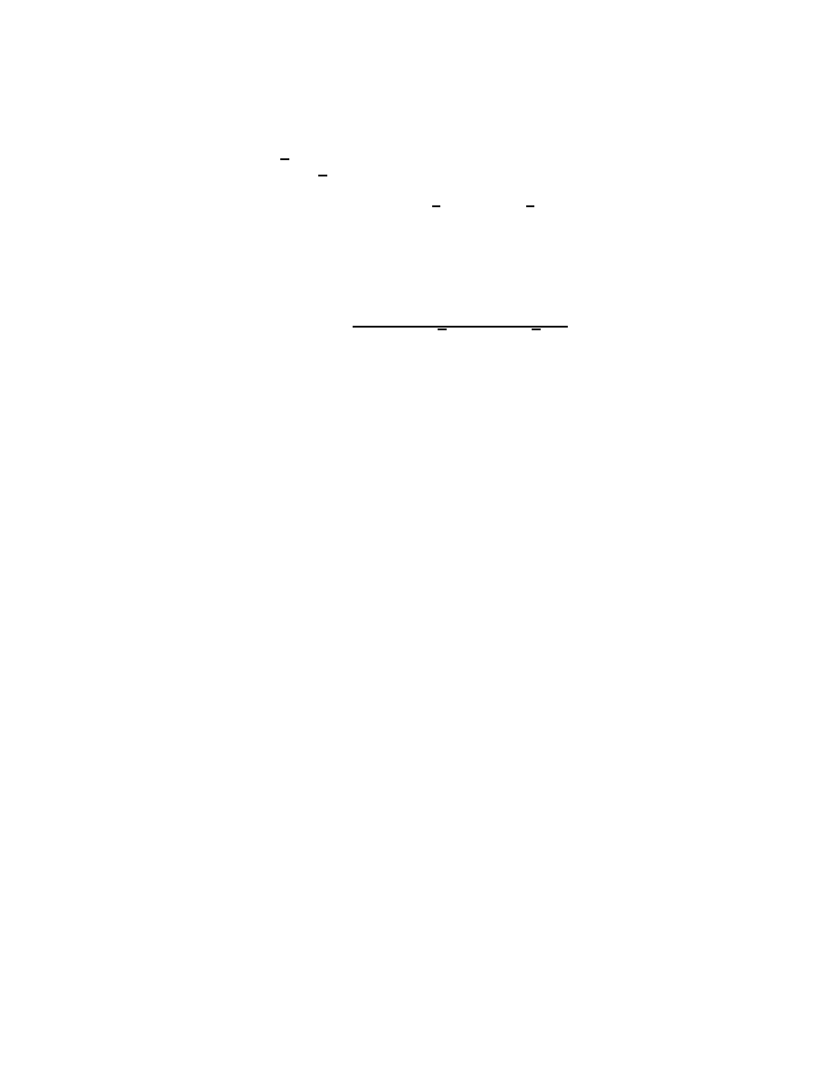
38
Chapter 12. Sequential Equilibrium
where P
β
0
(a) is the product of the probabilities assigned by β
0
to the sequence a of actions.
Now for all h
0
∈ I
0
i
let h(h
0
) be the subhistory of h
0
in I
i
(existence and uniqueness follows
from perfect recall). Let h
0
\ h(h
0
) be the part of h
0
subsequent to I
i
. Then,
Pr(β
0
, µ|I
i
)(I
0
i
) =
X
h
0
∈I
0
i
µ(I
i
)(h(h
0
)) · P
β
0
(h
0
\ h(h
0
)).
Since (β, µ) is consistent there is a sequence of completely mixed assessments (β
n
, µ
n
) with
µ
n
→ µ and β
n
→ β as n → ∞ and for all n the belief µ
n
is derived from β
n
using Bayes’
rule. For each n we have
µ
n
(I
0
i
)(ˆ
h, a
0
) =
µ
n
(I
i
)(ˆ
h) · P
β
0
(a
0
)
P
h
0
∈I
i
µ
n
(I
i
)(h(h
0
)) · P
β
0
(h
0
\ h(h
0
))
since Pr(β
0
, µ|I
i
)(I
0
i
) > 0. Taking the limit as n → ∞ and using P
β
0
(a
0
, a
00
) = P
β
0
(a
0
)·P
β
0
(a
00
)
we conclude that O(β
0
, µ|I
i
)(h) = O(β
0
, µ|I
0
i
)(h) · Pr(β
0
, µ|I
i
)(I
0
i
).
To show the one deviation property, use backwards induction. Suppose that (β, µ) is
a consistent assessment with the property that no player has an information set at which
a change in his action (holding the remainder of his strategy fixed) increases his expected
payoff conditional on reaching that information set. Take an information set I
i
of player i
and suppose that β
i
is optimal conditional on reaching any of the information sets I
0
i
of
player i that immediately follow I
i
. We need to show that β
i
is optimal conditional on
reaching I
i
. Suppose that player i uses the strategy β
0
i
. Let β
0
= (β
−i
, β
0
i
), let F (I
i
) be the
set of information sets of player i that immediately follow I
i
, and let Z(I
i
) be the set of
terminal histories that have subhistories in I
i
. Then player i’s expected payoff conditional on
reaching I
i
is the sum of his payoffs to histories that do not reach another of his information
sets, say E
i
, and
X
I
0
i
∈F (I
i
)
X
h∈Z(I
0
i
)
O(β
0
, µ|I
i
)(h) · u
i
(h).
This is equal, using the equality in the first part of the problem, to
E
i
+
X
I
0
i
∈F (I
i
)
X
h∈Z(I
0
i
)
O(β
0
, µ|I
0
i
)(h) · Pr(β
0
, µ|I
i
)(I
0
i
) · u
i
(h),
which is equal to
E
i
+
X
I
0
i
∈F (I
i
)
Pr(β
0
, µ|I
i
)(I
0
i
) · E
(β
0
,µ)
[u
i
|I
0
i
],
where E
(β
0
,µ)
[u
i
|I
0
i
] is the expected payoff under (β
0
, µ) conditional on reaching I
0
i
, which by
the induction assumption is at most
E
i
+
X
I
0
i
∈F (I
i
)
Pr(β
0
, µ|I
i
)(I
0
i
) · E
(β,µ)
[u
i
|I
0
i
].
Now, again using the equality in the first part of the problem, this is equal to
E
((β
−i
, ˆ
β
i
),µ)
[u
i
|I
i
],
where ˆ
β
i
is the strategy of player i in which player i uses β
0
i
at I
i
and β
i
elsewhere. Thus
β
i
is optimal conditional on reaching I
i
.

Chapter 12. Sequential Equilibrium
39
229.1 (Non-ordered information sets) The three sequential equilibria are:
• Strategies β
1
(s) = 1, β
2
(d) = 1, β
3
(s) = 1.
Beliefs
µ
1
(a) = 1, µ
2
(a, c) = µ
2
(b, e) =
1
2
, µ
3
(b) = 1.
• Strategies β
1
(c) = 1, β
2
(`) = 1, β
3
(e) = 1.
Beliefs
µ
1
(a) = 1, µ
2
(a, c) = µ
2
(b, e) =
1
2
, µ
3
(b) = 1.
• Strategies β
1
(c) = 1, β
2
(r) = 1, β
3
(e) = 1.
Beliefs
µ
1
(a) = 1, µ
2
(a, c) = µ
2
(b, e) =
1
2
, µ
3
(b) = 1.
It is straightforward to check that each of these assessments satisfies sequential rationality
and consistency.
The first equilibrium has the following undesirable feature. Player 2’s strategy d is
optimal only if he believes that each of the two histories in his information set occurs with
probability
1
2
. If he derives such a belief from beliefs about the behavior of players 1 and 3
then he must believe that player 1 chooses c with positive probability and player 3 chooses
e with positive probability. But then it is no longer optimal for him to choose d: ` and r
both yield him 2, while d yields less than 2. That is, any alternative strategy profile that
rationalizes player 2’s belief in the sense of structural consistency makes player 2’s action in
the sequential equilibrium suboptimal.
Nevertheless, player 2’s strategy can be rationalized by another explanation of the rea-
son for reaching the information set. Assume that player 2 believes that players 1 and 3
attempted to adhere to their behavioral strategies but made errors in carrying out these
strategies. Then the fact that he believes that there is an equal probability that each of
them made a mistake does not mean that he has to assign a positive probability to a mistake
in the future.
234.2 (Sequential equilibrium and PBE ) Since (β, µ) is a sequential equilibrium there is a sequence
(β
n
, µ
n
)
∞
n=1
of assessments that converges to (β, µ) and has the properties that each strategy
profile β
n
is completely mixed and each belief system µ
n
is derived from β
n
using Bayes’ law.
For each h ∈ H, i ∈ P (h), and θ
i
∈ Θ
i
let σ
n
i
(θ
i
)(h) = β
n
i
(I(θ
i
, h)) for each value of n. Given
these (completely mixed) strategies define a profile (µ
n
i
) of beliefs in the Bayesian extensive
game that satisfies the last three conditions in Definition 232.1. It is straightforward to
show that µ
n
(I(θ
i
, h))(θ, h) = Π
j∈N \{i}
µ
n
j
(h)(θ
j
) for each value of n. This equality and the
properties of (µ
n
i
) are preserved in the limit, so that µ(I(θ
i
, h))(θ, h) = Π
j∈N \{i}
µ
j
(h)(θ
j
).
Thus by the sequential rationality of the sequential equilibrium, ((σ
i
), (µ
i
)) is sequentially
rational and hence a perfect Bayesian equilibrium.
237.1 (Bargaining under imperfect information) Refer to the type of player 1 whose valuation
is v as type v. It is straightforward to check that the following assessment is a sequential
equilibrium: type 0 always offers the price of 2 and type 3 always offers the price of 5.
In both periods player 2 accepts any price at most equal to 2 and rejects all other prices
(regardless of the history). If player 2 observes a price different from 5 in either period then
he believes that he certainly faces type 0. (Thus having rejected a price of 5 in the first
period, which he believed certainly came from type 3, he concludes, in the event that he
observes a price different from 5 in the second period, that he certainly faces type 0.)
Comment
There are other sequential equilibria, in which both types offer a price between
3 and 3.5, which player 2 immediately accepts.

40
Chapter 12. Sequential Equilibrium
238.1 (PBE is SE in Spence’s model ) It is necessary to show only that the assessments are con-
sistent. Consider the pooling equilibrium. Suppose that a type θ
L
1
worker chooses e
∗
with
probability 1 − and distributes the remaining probability over other actions, while a
type θ
H
1
worker chooses e
∗
with probability 1 −
2
and distributes the remaining probability
2
over other actions. The employer’s belief that these completely mixed strategies induce
converges to the one in the equilibrium as → 0, so that the equilibrium assessment is
indeed consistent. A similar argument shows that the separating equilibrium is a sequential
equilibrium.
243.1 (PBE of chain-store game) The challengers’ beliefs are initially correct and action-determined,
and it is shown in the text that the challengers’ strategies are sequentially rational, so that
it remains to show that the chain-store’s strategy is sequentially rational and that the chal-
lengers’ beliefs satisfy the condition of Bayesian updating.
Sequential rationality of regular chain-store’s strategy
:
• If t(h) = K then the regular chain-store chooses C, which is optimal.
• Suppose that t(h) = k ≤ K − 1 and µ
CS
(h)(T ) ≥ b
K−k
. Then if the chain-store
chooses C it obtains 0 in the future. If it chooses F then challenger k + 1 believes
that the probability that the chain-store is tough is max{b
K−k
, µ
CS
(h)(T )} and stays
out. Thus if the chain-store chooses F then it obtains −1 against challenger k and a
against challenger k + 1. Thus it is optimal to choose F .
• Suppose that t(h) = k ≤ K − 1 and µ
CS
(h)(T ) < b
K−k
. Then if the chain-store
chooses C it obtains 0 in the future. If it chooses F then challenger k + 1 believes
that the probability that the chain-store is tough is max{b
K−k
, µ
CS
(h)(T )} = b
K−k
and chooses Out with probability 1/a. Thus if the chain-store chooses F against
challenger k and challenger k + 1 chooses Out then the chain-store obtains a total
payoff of −1 + a · (1/a) = 0 when facing these two challengers. If the chain-store
chooses F against challenger k and challenger k + 1 chooses In then the chain-store
randomizes in such a way that it obtains an expected payoff of 0 regardless of its future
actions. Thus the chain-store’s expected payoff if it chooses F against challenger k is
zero, so that it is optimal for it to randomize between F and C.
Sequential rationality of tough chain-store’s strategy
: If the tough chain-store chooses
C after any history then all future challengers enter. Thus it is optimal for the tough
chain-store to choose F .
Bayesian updating of beliefs
:
• If k ≤ K −1 and µ
CS
(h)(T ) ≥ b
K−k
then both types of chain-store fight challenger k if
it enters. Thus the probability µ
CS
(h, h
k
)(T ) assigned by challenger k+1 is µ
CS
(h)(T )
when h
k
= (In, F ).
• If k ≤ K − 1 and µ
CS
(h)(T ) < b
K−k
then the tough chain-store fights challenger k
if it enters and the regular chain-store accommodates with positive probability p
k
=
(1 − b
K−k
)µ
CS
(h)(T )/((1 − µ
CS
(h)(T ))b
K−k
). Thus in this case
µ
CS
(h, h
k
)(T ) =
µ
CS
(h)(T )
µ
CS
(h)(T ) + (1 − µ
CS
(h)(T ))p
k
= b
K−k
if h
k
= (In, F ).

Chapter 12. Sequential Equilibrium
41
• If µ
CS
(h)(T ) = 0 or h
k
= (In, C), k ≤ K − 1, and µ
CS
(h)(T ) < b
K−k
then we have
µ
CS
(h, h
k
)(T ) = 0 since only the regular chain-store accommodates in this case.
• If h
k
= (In, C), k ≤ K − 1, and µ
CS
(h)(T ) ≥ b
K−k
then neither type of chain-store
accommodates entry, so that if C is observed challenger k + 1 can adopt whatever
belief it wishes; in particular it can set µ
CS
(h, h
k
)(T ) = 0.
246.2 (Pre-trial negotiation) The signaling game is the Bayesian extensive game with observ-
able actions hΓ, (Θ
i
), (p
i
), (u
i
)i in which Γ is a two-player game form in which player 1 first
chooses either 3 or 5 and then player 2 chooses either Accept or Reject ; Θ
1
= {Negligent, Not },
Θ
2
is a singleton, and u
i
(θ, h) takes the values described in the problem.
The game has no sequential equilibrium in which the types of player 1 make different
offers. To see this, suppose that the negligent type offers 3 and the non-negligent type offers
5. Then the offer of 3 is rejected and the offer of 5 is accepted, so the negligent player 1
would be better off if she offered 5. Now suppose that the negligent type offers 5 and the
non-negligent type offers 3. Then both offers are accepted and the negligent type would be
better off if she offered 3.
The only sequential equilibria in which the two types of player 1 make the same offer
are as follows.
• If p
1
(Not ) ≥
2
5
then the following assessment is a sequential equilibrium. Both types
of player 1 offer the compensation of 3 and player 2 accepts any offer. If the com-
pensation of 3 is offered then player 2 believes that player 1 is not negligent with
probability p
1
(Not ); if the compensation 5 is offered then player 2 may hold any belief
about player 1. (The condition p
1
(Not ) ≥
2
5
is required in order for it to be optimal
for player 2 to accept when offered the compensation 3.)
• For any value of p
1
(Not ) the following assessment is a sequential equilibrium. Both
types of player 1 offer the compensation 5; player 2 accepts an offer of 5 and rejects an
offer of 3. If player 2 observes the offer 3 then he believes that player 1 is not negligent
with probability at most
2
5
.
Consider the case in which p
1
(Not ) >
2
5
. The second type of equilibrium involves the
possibility that if player 1 offers only 3 then the probability assigned by player 2 to her being
negligent is increasing. A general principle that excludes such a possibility emerges from the
assumption that whenever it is optimal for a negligent player 1 to offer the compensation 3
it is also optimal for a non-negligent player 1 to do so. Thus if the out-of-equilibrium offer 3
is observed a reasonable restriction on the belief is that the relative probability of player 1
being non-negligent should increase and thus exceed
2
5
. However, if player 2 holds such a
belief then his planned rejection is no longer optimal.
252.2 (Trembling hand perfection and coalescing of moves) In the original game the history (L, R)
is an outcome of a trembling hand perfect equilibrium in which player 1 chooses (L, r) and
player 2 chooses R. If we coalesce player 1’s moves then we get the game in which player 1
chooses between the three actions L, R`, and Rr. In this game the only trembling hand
perfect equilibrium is (Rr, R).
Comment
If the game is modifies so that the payoffs of player 2 to the history (L, R) and
(R, r) remain positive but are different then coalescing player 1’s moves affects the players’
equilibrium payoffs.
42
Chapter 12. Sequential Equilibrium
b
1
1
2
XXXX
X
XXXX
XXXX
XX
X
r
r
r
r
r
@
@
r
2, 2
0, 1
r
g
b
r
@
@
r
2, 2
0, 1
r
g
b
r
@
@
r
2, 2
1, 0
r
g
b
r
@
@
r
2, 2
1, 0
r
g
b
p
p
p
p
p
p
p
p
p
p
p
p
p
p
p
p
p
p
p
p
p
p
p
p
p
p
p
p
p
p
2
1
2
p
p
p
p
p
p
p
p
p
p
p
p
1 (.5)
2 (.5)
1
2
1
2
c
2,2
Figure 42.1 The extensive form of the game in Exercise 253.1
1
2g
2b
1g
2, 2
2, 2
3
2
, 1
1b
0, 1
1,
3
2
1
2
,
1
2
2
2, 2
2, 2
1, 0
Figure 42.2 The reduced strategic form of the game in Figure 42.1.
253.1 (Example of trembling hand perfection) The extensive form of the game is given in Fig-
ure 42.1.
The reduced strategic form is shown in Figure 42.2. The only strategies that are not
weakly dominated are 1g for player 1 and 2g for player 2. Thus by Proposition 248.2 the
strategy profile (1g, 2g) is the unique trembling hand perfect equilibrium of the strategic
form of the game.
We now argue that ((1, g), (2, g)) is not a trembling hand perfect equilibrium of the
extensive game. By definition, a trembling hand perfect equilibrium of the extensive game
corresponds to a trembling hand perfect equilibrium of the agent strategic form of the
game. Consider a completely mixed strategy profile of the agent strategic form of the game.
Assume that the probability with which player 1’s second agent chooses b is at least as
large as the probability with which player 2’s second agent chooses b. Then the only best
response of player 1’s first agent is to choose 2. To see this, let p
i
be the probability with
which player i’s first agent chooses i and let q
i
be the probability that player i’s second
agent chooses g. Then player 1’s payoff if her first agent chooses 1 is
(1 − p
2
) · 2q
1
+ p
2
· [
1
2
· 2q
1
+
1
2
(2q
2
+ 1 − q
2
)]
while her payoff if her first agent chooses 2 is
(1 − p
2
) · 2 + p
2
· [2q
2
+ 1 − q
2
].
The difference between the first and second of these payoffs is
2(1 − p
2
)(q
1
− 1) + p
2
· [q
1
− q
2
−
1
2
(1 − q
2
)] < 0
if q
2
≥ q
1
. A symmetric argument applies to player 2’s first agent. Thus given any completely
mixed strategy profile, for at least one player it is better for that players’s first agent to
choose the other player.

Chapter 12. Sequential Equilibrium
43
Interpretation
: Trembling hand perfect equilibrium in the strategic form captures the
idea that each player is concerned about (small) mistakes that his opponent may make,
which leads each player in this game to choose himself to be the one to make the decision.
Trembling hand perfect equilibrium in the extensive game allows for the fact that the player
may make mistakes himself in carrying out his strategy later in the game, which in this
game, given that errors by oneself are more costly than errors by one’s opponent, militates
against choosing oneself to be the decision-maker.


13
The Core
259.3 (Core of production economy) First suppose that the payoff profile x is a member of the set
given. If S does not contain the capitalist then v(S) = 0, so certainly x(S) ≥ v(S). If S does
contain the capitalist then x(S) = f (w)−
P
i∈N \S
x
i
≥ f (w)−(w+1−|S|)(f (w)−f (w−1)),
which is at least f (|S|) by the concavity of f . Thus x is in the core.
Now suppose that x is a feasible payoff profile for which x
i
> f (w) − f (w − 1) for some
i 6= c. Then x(N \ {i}) = f (w) − x
i
< f (w) − (f (w) − f (w − 1)) = f (w − 1) = v(N \ {i}),
so that x is not in the core.
In each payoff profile in the core each worker receives not more than his marginal product
when all workers are employed, and the capitalist receives the residual.
260.2 (Market for indivisible good ) Let x be a payoff profile in the core, let b be a buyer whose
payoff is minimal among the payoffs of all the buyers, and let ` be a seller whose payoff
is minimal among the payoffs of all the sellers. Then x
b
+ x
`
≥ v({b, `}) = 1; since |L| =
v(N ) ≥ |B|x
b
+ |L|x
`
= |L|(x
b
+ x
`
) it follows that x
b
+ x
`
= 1 and x
i
= x
j
if i and j
are both buyers or if they are both sellers. Thus the core is the set of all payoff profiles
in which for some α ∈ [0, 1] every buyer receives the payoff α and every seller receives the
payoff 1 − α. That is, any split of the surplus is possible in this case; the only impact of the
competition between buyers and between sellers is that all pairs must split in the same way.
260.4 (Convex games) Let S
∗
= {i
1
, . . . , i
|S
∗
|
} be any coalition, with i
1
< · · · < i
|S
∗
|
. Then
x
i
1
= v(S
i
1
∪ {i
1
}) − v(S
i
1
) ≥ v({i
1
}) (take S = S
i
1
and T = {i
1
} in the definition of
convexity). But then x
i
1
+ x
i
2
≥ v({i
1
}) + v(S
i
2
∪ {i
2
}) − v(S
i
2
) ≥ v({i
1
, i
2
}) (take S = S
i
2
and T = {i
1
, i
2
} in the definition of convexity). Continuing similarly we reach the conclusion
that x
i
1
+ . . . + x
i
|S∗ |
≥ v(S
∗
). Further,
P
i∈N
x
i
= v(N ), so that x is in the core of hN, vi.
261.1 (Simple games)
a
. For each i ∈ N let S
i
be a winning coalition that does not contain i; let x be a payoff
profile in the core. Then
x(N \ {i}) ≥ x(S
i
) ≥ v(S
i
) = 1,
so that
P
i∈N
x(N \ {i}) ≥ |N |. On the other hand
X
i∈N
x(N \ {i}) = (|N | − 1)
X
i∈N
x
i
= |N | − 1,

46
Chapter 13. The Core
a contradiction.
b
. Let V be the set of veto players. Let x be a nonnegative feasible payoff profile for
which x
i
= 0 for all i ∈ N \ V . If S is not a winning coalition then v(S) = 0 so that certainly
x(S) ≥ v(S); if S is a winning coalition then x(S) = 1 = v(S). Thus x is in the core. Now,
if x is in the core then since v(S) ≥ 0 for all S we have x
i
≥ 0 for all i ∈ N . Let x be a
feasible payoff profile for which x
i
> 0 for some i ∈ N \ V . Let S be a winning coalition
that does not include i. Then x(S) < 1 = v(S), so that x is not in the core.
261.2 (Zerosum games) If hN, vi is zerosum and x is in the core of hN, vi then for any coalition
S we have x(S) ≥ v(S) and x(N \ S) ≥ v(N \ S); since x(S) + x(N \ S) = x(N ) = v(N ) =
v(S) + v(N \ S) it follows that x(S) = v(S). Thus for all disjoint coalitions S and T we
have v(S) + v(T ) = x(S) + x(T ) = x(S ∪ T ) = v(S ∪ T ). Hence hN, vi is additive.
261.3 (Pollute the lake)
a
. Let S be a coalition and let |S| = s. The payoff of S is minimized if none of the
members of N \ S treats its waste. In this case the payoff of S if k of its members treat
their waste is −s(n − k)c − kb. Thus if sc ≥ b then the payoff of S is maximized when all
members of S treat their waste, yielding S a payoff of −s(n − s)c − sb, and if sc ≤ b then
the payoff of S is maximized when no member of S treats its waste, yielding S a payoff of
−snc. Thus
v(S) =
−snc
if s < b/c
−s[(n − s)c + b] if s ≥ b/c.
b
. First we argue that since the game is symmetric the core is nonempty if and only if it
contains the payoff profile x = (−b, . . . , −b). To see this, suppose that x is not in the core.
Then for some integer k such that v(S) > −kb for every coalition S with |S| = k. Now
let y 6= x be a feasible payoff profile. Then there exists some coalition T with |T | = k and
y(T ) < −kb = v(T ). Thus y is not in the core.
Now, if |S| = s ≤ b/c then x(S) = −sb ≥ −snc = v(S) and if |S| = s > b/c then
x(S) = −sb ≥ −s[(n − s)c + b] = v(S) and x(N ) = −nb = v(N ) (by the assumption that
b ≤ nc). Thus x is in the core of the game, which consequently is always nonempty.
The core is a singleton if and only if b = nc. To show this, first suppose that b = nc
and x 6= (−b, . . . , −b). Then x
i
< −b for some i ∈ N , so that x({i}) < v({i}) = −nc = −b
(since c ≤ b); thus x is not in the core. Conversely, if b < nc and x = (−b, . . . , −b) then
x(S) > v(S) whenever |S| < n, so that the core contains payoff profiles different from x.
c
. Under the assumptions in the exercise a coalition is pessimistic about the outcome
when it deviates, and consequently does so only when it is sure that it can increase its payoff
from doing so. The value of v(S) for each S 6= N is smaller than it is under alternative
assumptions, causing the core to be larger than it is under alternative assumptions.
263.2 (Game with empty core) Let λ
{1,2}
= λ
{1,3}
= λ
{1,4}
=
1
3
and λ
{2,3,4}
=
2
3
. Then (λ
S
) is a
balanced collection of weights; since
1
3
v({1, 2}) +
1
3
v({1, 3}) +
1
3
v({1, 4}) +
2
3
v({2, 3, 4}) =
5
4
> v(N ) the game is not balanced and thus (by the Bondareva–Shapley theorem) has an
empty core.
265.2 (Syndication in a market )
a
. We have v(S) = min{2|S ∩ {1, 2}|, |S ∩ {3, 4, 5}|} for each coalition S. If x is in the
core then x
1
+ x
i
+ x
j
≥ 2 whenever {i, j} ⊆ {3, 4, 5}, so that 3x
1
+ 2(x
3
+ x
4
+ x
5
) ≥ 6 and

Chapter 13. The Core
47
hence x
1
≥ 2x
2
(using x
3
+ x
4
+ x
5
= 3 − x
1
− x
2
). Similarly x
2
≥ 2x
1
, so that x
1
= x
2
= 0.
We also require x
1
+ x
i
≥ 1 if i ∈ {3, 4, 5}, so that the core is {(0, 0, 1, 1, 1)}.
b
. Let the players be 1, 2, and s (the syndicate). We have v({1, s}) = v({2, s}) = 2,
v(N ) = 3, and v(S) = 0 otherwise. The core is the set of feasible payoff profiles for which
0 ≤ x
1
≤ 1 and 0 ≤ x
2
≤ 1. Thus the core predicts that the members of the syndicate are
never better off, and may be worse off. An interpretation is that the fact that 3, 4, and 5
always act as a block dulls the competition between 1 and 2, who cannot now compete with
each other by forming (efficient) coalitions consisting of only two of the three members of
3, 4, and 5. (The payoff profile (1, 1,
1
3
,
1
3
,
1
3
) is not in the core of the unsyndicated market
since the coalition {1, 3, 4} can obtain 2 units of payoff.)
267.2 (Existence of competitive equilibrium in market) First note that the two sets are nonempty
and convex and their interiors are disjoint, so that indeed they can be separated. Thus there
exists (α, β) ∈ R
`
× R, not equal to 0, such that
α · z + βy ≤ α ·
X
i∈N
z
∗
i
+ β
X
i∈N
f
i
(z
∗
i
) for all (z, y) ∈ X.
Since (
P
i∈N
z
∗
i
+ 1
j
,
P
i∈N
f
i
(z
∗
i
)) ∈ X, where 1
j
is the jth unit vector, we have α
j
≤ 0 for
all j. We now show that β > 0. Since
P
i∈N
ω
i
> 0 there exists ∈ R
`
++
and δ > 0 such
that (
P
i∈N
z
∗
i
− ,
P
i∈N
f
i
(z
∗
i
) − δ) ∈ X, so that −α · − βδ ≤ 0 or βδ ≥ −α · . If α = 0
then we conclude that β ≥ 0, and since (α, β) 6= 0 it follows that β > 0. If α
j
< 0 for some
j then we conclude directly that β > 0.
Now let p = −α/β ≥ 0. Since (
P
i∈N
z
∗
i
− z
∗
k
+ z
k
,
P
i∈N
f
i
(z
∗
i
) − f
k
(z
∗
k
) + f
k
(z
k
)) ∈ X
for any z
k
∈ R
`
+
we have
f
k
(z
∗
k
) − pz
∗
k
≥ f
k
(z
k
) − pz
k
for all z
k
∈ R
`
+
,
so that (p, (z
∗
i
)
i∈N
) is a competitive equilibrium.
Comment
This is not an exercise in game theory.
268.1 (Core convergence in production economy) In all elements of the core the payoff of every
player i 6= 1 is at most f (1, k) − f (1, k − 1) (see Exercise 259.3). Now, the concavity of
f (1, k) implies that k(f (1, k) − f (1, k − 1)) ≤ 2(f (1, k) − f (1, k/2)) (since
f (1, k) − f (1, k/2) =
k
X
j=k/2+1
(f (1, j) − f (1, j − 1))
≥
k
X
j=k/2+1
(f (1, k) − f (1, k − 1))
≥ (k/2)[f (1, k) − k(1, k − 1)]).
Since f is bounded we have f (1, k) − f (1, k/2) → 0, establishing the result.
Interpretation: Competition between the workers drives their payoff down to their
marginal product, which declines to zero, so that the single capitalist gets all the surplus.

48
Chapter 13. The Core
274.1 (Core and equilibria of exchange economy) We first claim that the only competitive price
is (p
1
, p
2
) = (
1
2
,
1
2
). To see this, suppose that p
1
> p
2
; then each agent of type 1 demands
none of good 1 and each agent of type 2 demands less than
1
2
a unit of good 1, so that the
aggregate demand for good 1 is less than the supply. If p
1
< p
2
then each agent of type 1
demands 1 unit of good 1 and each agent of type 2 demands more than
1
2
a unit of good 1,
so that the aggregate demand for good 1 exceeds the supply. An allocation is competitive
if each agent i of type 1 obtains the bundle (y
i
, 1 − y
i
) for some y
i
∈ [0, 1] and each agent
of type 2 obtains the bundle (
1
2
,
1
2
), where
P
i
of type
1
y
i
= k/2.
Now consider the core. First suppose that k = 1. In order for the allocation ((s, t), (1 −
s, 1−t)) to be in the core we require s+t ≥ 1 (considering the coalition {1}) and 1−s = 1−t
(considering the coalition {1, 2}). Thus the core consists of all allocations ((s, s), (1−s, 1−s))
for which s ≥
1
2
.
Now suppose that k ≥ 2. We claim that the core of kE is the set of competitive
allocations. We show this as follows. Let x be an allocation in the core.
Step 1
. For each agent i of type 2 we have x
i
= (y
i
, y
i
) for some y
i
∈ [0, 1]. The argument
is straightforward.
Step 2
. Each agent obtains the same payoff. The argument is the same as that for
Lemma 272.2 (the equal treatment result).
Step 3
. Each agent of type 2 obtains the same bundle. This follows from Steps 1 and 2.
Step 4
. Each agent of type 2 obtains the bundle (
1
2
,
1
2
). By Steps 1, 2, and 3 each agent
of type 2 obtains the same bundle (y, y) with y ≤
1
2
. Suppose that y <
1
2
. Then each agent
of type 1 obtains the payoff 2(1 − y). Consider a coalition S that consists of one agent of
type 1 and two agents of type 2. The endowment of S is (1, 2), so that it is feasible to give
the agent of type 1 the bundle (1 − 2y − 2, 2 − 2y − 2) and each agent of type 2 the bundle
(y + , y + ) if > 0 is small enough. In this allocation the payoff of each agent exceeds his
payoff in the original allocation if is small enough, establishing the result.
Finally, it is easy to show that each allocation in which each agent i of type 1 obtains
the bundle (y
i
, 1 − y
i
) for some y
i
∈ [0, 1] and each agent of type 2 obtains the bundle (
1
2
,
1
2
)
is indeed in the core.

14
Stable Sets, the Bargaining Set, and
the Shapley Value
280.1 (Stable sets of simple games) Let Y be the set of imputations described in the problem. To
show internal stability let y ∈ Y and suppose that z
S
y for some z ∈ Y . Then z
i
> y
i
≥ 0
for all i ∈ S, so that z(S) > y(S). Since z ∈ Y we have S ⊆ T ; since S is winning and T
is minimal winning we have T ⊆ S. Thus z(S) = y(S), a contradiction. To show external
stability let z ∈ X \ Y . Then
P
i∈T
z
i
< 1 so that there exists y ∈ Y such that y
T
z.
280.2 (Stable set of market for indivisible good )
Internal stability
: Let y ∈ Y and suppose that z ∈ Y with z
i
> y
i
for all i ∈ S. Then
S ⊆ L or S ⊆ B; but then v(S) = 0.
External stability
: Let z ∈ X \ Y . Let i be the buyer whose payoff is lowest among
all buyers, let j be the seller whose payoff is lowest among all sellers, let z
b
be the average
payoff of the buyers in z, and let z
`
be the average payoff of the sellers. Since |B|z
b
+ |L|z
`
=
v(N ) = |L| we have z
b
= (1 − z
`
)|L|/|B|. Let y be the member of Y in which every buyer’s
payoff is z
b
and every seller’s payoff is z
`
. We have y
i
= z
b
≥ z
i
and y
j
= z
`
≥ z
j
, with at
least one strict inequality. Further, y
i
+ y
j
= z
b
+ z
`
= (1 − z
`
)|L|/|B| + z
`
≤ 1 = v({i, j}).
If we adjust y
i
and y
j
slightly to make both of the inequalities y
i
≥ z
i
and y
j
≥ z
j
strict
then y
{i,j}
z.
The standard of behavior that this stable set exhibits is “equality among agents of
the same type”. Note the difference between this set and a set of the type Y
p
= {x
i
=
p for all i ∈ L and x
j
= 1 − p for |L| members of B} for some p, which can be interpreted
as the standard of behavior “the price is p”.
280.3 (Stable sets of three-player games) The set of imputations is the triangle in Figure 50.1. The
core is the heavy line segment at the top of the diagram: the set {(γ, 0, 1 − γ): β ≤ γ ≤ 1}.
We know that the core is a subset of every stable set, so that (by internal stability) no
imputation that is dominated by a member of the core is a member of any stable set. The
set of imputations dominated by a member of the core (via the coalition {1, 3}) is shown in
the figure. Now take any of the remaining imputations, say x. The set of imputations that
it dominates is the union of the two shaded sets below the horizontal line through it. Thus
in order for external stability to be satisfied a stable set must contain every point on some
curve joining (β, 0, 1 − β) and the bottom of the triangle. In order for internal stability to be
satisfied a stable set can contain only the points on such a line, and the line must have the
property that all the points on it below any given point must lie between the two straight
50
Chapter 14. Stable Sets, the Bargaining Set, and the Shapley Value
J
J
J
J
J
J
J
J
J
J
J
J
J
J
J
J
J
J
J
J
J
J
J
JJ
J
J
JJ
J
J
J
J
J
J
J
J
J
J
J
J
J
J
J
J
J
J
J
J
J
J
J
J
J
J
J
J
J
J
J
J
J
J
J
J
J
J
J
J
J
J
J
J
J
J
J
J
J
J
J
J
J
J
J
J
J
J
J
J
J
J
J
J
J
J
J
J
J
J
J
J
J
J
J
J
qx
(0, 0, 1)
(0, 1, 0)
(1, 0, 0)
(β, 0, 1 − β)
)
Imputations dominated
by a member of the core
)
Imputations y for
which x
{1
,
3
}
y
PPP
q
Imputations y for
which x
{1
,
2
}
y
PPPP
q
core
Figure 50.1 The core and a stable set of the three-player game in Exercise 280.3. The
triangle is the set of imputations; each corner corresponds to an imputation in which one
player obtains a payoff of 1, as labelled. The heavy line at the top of the figure is the core,
and the core together with a curved line like the one shown is a stable set. (The curved line
extends from (β, 0, 1 − β) to the line x
1
= 0 and has the property that all points below any
given point on the line lie between the two straight lines through the point parallel to the
sloping sides of the triangle.)
lines through the point that are parallel to the sloping sides of the triangle. For example,
one stable set consists of the union of the points in the core and the points on the curved
line in the figure.
In the core player 2, the buyer with the lower reservation value, obtains nothing. One
interpretation of a stable set is that it corresponds to a method of splitting the joint payoff
that the buyers can obtain, with the following property: each dollar up to 1− β goes entirely
to player 3; a nonnegative amount of every subsequent dollar is added to the payoff of both
player 2 and player 3.
280.4 (Dummy’s payoff in stable sets) Let x be an imputation in a stable set and let i be a
dummy. Suppose that x
i
> v({i}) for some i ∈ N . Since v(N ) − v(N \ {i}) = v({i})
we have x(N \ {i}) < x(N ) − v({i}) = v(N ) − v({i}) = v(N \ {i}), so that there exists
an imputation y such that y
N \{i}
x. By internal stability we have y /
∈ Y , and thus by
external stability there exists an imputation z ∈ Y and a coalition S with z
S
y. If i /
∈ S
then we have z
S
x, contradicting internal stability; if i ∈ S then z
S\{i}
x since i is a
dummy, again contradicting internal stability. Thus x
i
= v({i}) for all i ∈ N .
280.5 (Generalized stable sets) It is straightforward to check that the core is a stable set. It is
the only stable set because it must be a subset of any stable set and every imputation not
in the core is dominated by an allocation in the core.
283.1 (Core and bargaining set of market ) Let x be an imputation; without loss of generality
assume that x
1
≤ x
2
and x
3
≤ x
4
≤ x
5
. We argue that x
1
= x
2
and x
3
= x
4
= x
5
. Assume
not; then either x
1
< x
2
or x
3
< x
5
and in either case x
2
+ x
5
> 1. In the arguments below
is a small enough positive number.

Chapter 14. Stable Sets, the Bargaining Set, and the Shapley Value
51
If x
1
+ x
3
< 1 and x
4
> 1 then consider the objection ((1 − x
3
− , x
3
+ ),{1, 3}) of 3
against 2. There is no counterobjection of 2 using either the coalition {2, 4} (since x
2
+ x
4
>
1) or the coalition {2, 4, 5} (since x
2
+ x
4
+ x
5
> 1). Adding player 1 to the counterobjecting
coalition does not increase its worth. Thus there is no counterobjection to the objection.
If x
1
+x
3
< 1 and x
4
≤ 1 then consider the objection (y, S) = ((1 − x
3
− 2,x
3
+ ,1 + ),
{1, 3, 4}) of 3 against 2. If is small enough there is no counterobjection of 2 using either
the coalition {2, 4} (since x
2
+ y
4
> 1) or the coalition {2, 4, 5} (since x
2
+ 1 − + x
5
> 0
for small enough). As before, adding player 1 to the counterobjecting coalition does not
increase its worth. Thus there is no counterobjection to the objection.
The remaining case is that in which x
1
+x
3
≥ 1. Since x
2
+x
5
> 1 we have x
1
+x
3
+x
4
<
2. Consider the objection ((x
1
+ , x
3
+ , 2 − x
1
− x
3
− 2), {1, 3, 4}) of 3 against 2. There is
no counterobjection of 2 using the coalition {2, 4} (since x
2
+ 2 − x
1
− x
3
− 2 > x
2
+ x
5
− 2,
which, for small enough, exceeds 1) or the coalition {2, 4, 5} (since x
2
+ 1 − + x
5
> 0 .
Thus there is no counterobjection to the objection.
We conclude that x
1
= x
2
= α and x
3
= x
4
= x
5
= β (say). For any objection of
1 against 2 using the coalition {1} ∪ S there is a counterobjection of 2 against 1 using
the coalition {2} ∪ S. Any objection of 3 against 4 or 5 can be countered similarly. Now
consider an objection of 1 against 3. If the coalition used is {1, 4} then 3 can counterobject
using {2, 3}; if the coalition used is {1, 4, 5} then 3 can counterobject using {2, 3, 4}; if the
coalition used is {1, 2, 4, 5} then 3 can counterobject using {2, 3, 4}. By similar arguments
any objection of 3 against 1 can be countered.
The core of the game consists of the single imputation (0, 0, 1, 1, 1), which is induced by
competition between 1 and 2. In any other imputation (α, α, β, β, β) we have α + β < 1,
so that a coalition consisting of a seller and a buyer can profitably deviate. According to
the reasoning of the players modeled by the bargaining set such a deviation will not occur
since whenever one buyer points out that she can get together with a seller and increase her
payoff the seller points out that he can get together with another buyer and do so, which
convinces the original buyer not to deviate.
289.1 (Nucleolus of production economy) Let x be the imputation described in the exercise. We
need to show that for every objection (S, y) to x there is a counterobjection T . Let (S, y)
be an objection to x. Let W = N \ {1} (the set of workers).
Suppose that S ⊆ W and y
i
< x
i
for some i ∈ W . Then T = {i} is a counterobjection:
x(T ) = x
i
> y
i
= y(T ) and e(T, y) = −y
i
> −x
i
≥ −|S|x
i
= e(S, x) (since x
i
= x
j
for all i,
j ∈ W ).
Suppose that S ⊆ W and y
i
≥ x
i
for all i ∈ W . Then y
1
< x
1
; suppose that y
j
> x
j
.
We claim that T = N \ {j} is a counterobjection. We have x(T ) = x(N ) − x
j
> x(N ) − y
j
=
y(N ) − y
j
= y(T ). Further
e(T, y) =
f (w − 1) − (f (w) − y
j
)
=
y
j
− (f (w) − f (w − 1))
>
x
j
− (f (w) − f (w − 1))
=
−
1
2
(f (w) − f (w − 1))
and e(S, x) = −
1
2
|S|(f (w) − f (w − 1)) ≤ −
1
2
(f (w) − f (w − 1)).
Suppose that S 3 1; let |S| = s+ 1. Since (S, y) is an objection to x we have y(S) > x(S)
and s < w. We claim that T = N \ S is a counterobjection. First note that y(T ) = f (w) −

52
Chapter 14. Stable Sets, the Bargaining Set, and the Shapley Value
y(S) and x(T ) = f (w) − x(S), so that y(T ) < x(T ). We now show that e(T, y) ≥ e(S, x),
so that T is a counterobjection to (S, y). We have
e(S, x)
=
f (s) − [f (w) − (w − s) ·
1
2
(f (w) − f (w − 1))]
=
f (s) −
2 − w + s
2
f (w) −
w − s
2
f (w − 1)
and
e(T, y) =
−y(T )
>
−x(T )
=
−(w − s) ·
1
2
(f (w) − f (w − 1))
≥
f (s) −
2 − w + s
2
f (w) −
w − s
2
f (w − 1),
since by the concavity of f we have f (w) − f (s) ≥ (w − s)(f (w) − f (w − 1)).
289.2 (Nucleolus of weighted majority games) We do not have any direct solution to this exercise.
(The result is taken from Peleg (1968), who provides a proof based on the standard definition
of the nucleolus.)
294.2 (Necessity of axioms for Shapley value)
a
. The arguments for DUM and ADD are the same as those for the Shapley value.
The value ψ does not satisfy SYM: let N = {1, 2} and consider the game v defined by
v({1, 2}) = 1 and v({1}) = v({2}) = 0. Players 1 and 2 are interchangeable but ψ
1
(v) = 0
and ψ
2
(v) = 1.
b
. The value ψ clearly satisfies SYM and ADD. It does not satisfy DUM: let N = {1, 2}
and consider the game v defined by v({1, 2}) = v({1}) = 1 and v({2}) = 0. Player 2 is a
dummy but ψ
2
(v) =
1
2
6= v({2}).
c
. The value ψ clearly satisfies SYM and DUM. The following example shows that it
does not satisfy ADD. Let N = {1, 2} and define v by v({1}) = 0 and v({2}) = v({1, 2}) = 1
and w by w({1}) = w({2}) = 0 and w({1, 2}) = 1. Then player 1 is a dummy in v, so that
ψ
1
(v) = 0, while ψ
1
(w) =
1
2
; we find that ψ
1
(v + w) = 1 > ψ
1
(v) + ψ
1
(w).
295.1 (Example of core and Shapley value) The core is {(1, 1, 1, 0)} since for any 1 ≤ i < j ≤ 3
we need x
i
+ x
j
≥ v({i, j}) = 2 in order for x to be in the core.
The Shapley value gives player 4 a payoff of
1
4
since his marginal contribution is positive
only in orderings in which he is last, and it is 1 in such an ordering. The other players are
symmetric, so that the Shapley value of the game is (
11
12
,
11
12
,
11
12
,
1
4
).
Player 4 obtains a payoff of 0 in the core, despite the fact that his presence makes a
difference to the amount of payoff that the other players can obtain. The reason is that the
core is sensitive to the demands of the two-player coalitions among players 1, 2, and 3, each
of which can obtain a payoff of 2 and player 4 needs at least two of these players to obtain
a positive payoff. The Shapley value, on the other hand, takes into account the “marginal
contribution” of each player to each possible coalition.
Chapter 14. Stable Sets, the Bargaining Set, and the Shapley Value
53
295.2 (Shapley value of production economy) The Shapley value gives player 1 (the capitalist)
a payoff of
P
w
i=1
f (i)/(w + 1) since in any ordering of the players in which she follows i
workers her marginal contribution is f (i) and the probability of her following i workers is
1/(w + 1). The workers are symmetric, so the Shapley value gives each of them a payoff of
(f (w) −
P
w
i=1
f (i)/(w + 1))/w.
295.4 (Shapley value of a model of a parliament)
a
. Let the two large parties be players 1 and 2. If n is large then each of the following
sets of orderings has probability close to
1
4
. A: Players 1 and 2 are both in the first half of
the ordering; B : Players 1 and 2 are both in the second half of the ordering; C : Player 1 is
in the first half of the ordering and player 2 in the second half; D : Player 1 is in the second
half of the ordering and player 2 is in the first half. The marginal contribution of player 1
is 0 except in orderings in A in which she comes after player 2 and in orderings in B in
which she comes before player 2, in which cases it is 1. Thus her expected contribution is
1
4
·
1
2
+
1
4
·
1
2
=
1
4
.
b
. The total share of the small parties is
1
2
if they are independent; if they unite then
the game is symmetric and they obtain only
1
3
.
295.5 (Shapley value of convex game) This follows from the result in Exercise 260.4, the definition
of the Shapley value, and the convexity of the core.
296.1 (Coalitional bargaining)
1
First we show that the strategy profile in which each player i ∈ S proposes x
i,S
whenever
the set of active players is S and each player j accepts a proposal y of player i when the set of
active players is S if and only if y
j
≥ x
S,i
j
is a subgame perfect equilibrium. It is immediate
that this acceptance rule is optimal. To show that player j’s proposals are optimal note that
by proposing x
S,j
he obtains x
S,j
j
; any proposal that gives him a higher payoff is rejected,
so that he obtains ρx
S
j
+ (1 − ρ)v({j}). Thus to complete the argument we need to show
that ρx
S
j
+ (1 − ρ)v({j}) ≤ x
S,j
j
, or
ρx
S
j
+ (1 − ρ)v({j}) ≤ v(S) − ρ
X
k∈S\{j}
x
S
k
− (1 − ρ)
X
k∈S\{j}
x
S\{j}
k
or
ρ
X
k∈S
x
S
k
+ (1 − ρ)v({j}) ≤ v(S) − (1 − ρ)
X
k∈S\{j}
x
S\{j}
k
.
Now,
P
k∈S
x
S
k
= v(S) and
P
k∈S\{j}
x
S\{j}
k
= v(S \{j}), so that the inequality follows from
the assumption that v(S ∪ {i}) ≥ v(S) + v({i}) for every coalition S and player i ∈ N \ S.
To show that there is a subgame perfect equilibrium for which x
S
= ϕ(S, v) for each
S ∈ C, let x
S,i
j
= ρϕ
j
(S, v)+(1−ρ)ϕ
j
(S\{i}, v) for each coalition S, i ∈ S, and j ∈ S\{i} and
x
S,i
i
= v(S) −
P
j∈S\{i}
x
S,i
j
. We have
P
j∈S\{i}
x
S,i
j
= ρ(v(S) − ϕ
i
(S, v)) + (1 − ρ)v(S \ {i}),
so that x
S,i
i
= (1 − ρ)(v(S) − v(S \ {i})) + ρϕ
i
(S, v). Further, using the fact that the
1
Correction to first printing
: After “active players” on line 5 add “, initially N ,”.

54
Chapter 14. Stable Sets, the Bargaining Set, and the Shapley Value
Shapley value satisfies the balanced contributions property we have x
S,i
j
= ϕ
j
(S, v) − (1 −
ρ)(ϕ
i
(S, v) − ϕ
i
(S \ {j}, v)) for j ∈ S \ {i}. Thus
X
i∈S
x
S,i
j
=
(|S| − 1)ϕ
j
(S, v) − (1 − ρ)(v(S) − ϕ
j
(S, v)) +
(1 − ρ)v(S \ {j}) + x
S,j
j
=
|S|ϕ
j
(S, v),
so that x
S
= ϕ(S, v) =
P
i∈S
x
S,i
/|S| as required.

15
The Nash Bargaining Solution
309.1 (Standard Nash axiomatization) See, for example, Osborne and Rubinstein (1990, pp. 13–
14).
309.2 (Efficiency vs. individual rationality) Fix α ∈ (0, 1) and consider the solution F defined by
F (X, D, %
1
,%
2
) ∼
i
α · N (X, D, %
1
, %
2
) for i = 1, 2, where N is the Nash solution.
Strict individual rationality: This follows from the fact that the Nash solution is strictly
individually rational.
SYM: Suppose that hX, D, %
1
, %
2
i is symmetric, with symmetry function φ. Since
F (X, D, %
1
,%
2
) ∼
i
α · N (X, D, %
1
, %
2
) we have
φ(F (X, D, %
1
,%
2
)) ∼
j
φ(α · N (X, D, %
1
, %
2
)) for j 6= i.
But
φ(α · N (X, D, %
1
, %
2
)) = α · φ(N (X, D, %
1
,%
2
)) = α · N (X, D, %
1
, %
2
).
Thus φ(F (X, D, %
1
,%
2
)) ∼
i
F (X, D, %
1
, %
2
) for i = 1, 2. Finally, from the non-redundancy
assumption we have φ(F (X, D, %
1
,%
2
)) = F (X, D, %
1
, %
2
).
IIA: Since N (X, D, %
0
1
, %
2
) = N (X, D, %
1
, %
2
) for preference relations that satisfy IIA
we have F (X, D, %
0
1
, %
2
) ∼
i
F (X, D, %
1
, %
2
). Thus from the non-redundancy assumption
F satisfies IIA.
What accounts for the difference between Roth’s result and the one here is that Roth’s
argument uses a comparison between two bargaining problems with different sets of agree-
ments, while here the set of agreements is fixed.
310.1 (Asymmetric Nash solution)
Well-definedness
: Suppose that u
i
and v
i
both represent player i’s preferences, for i = 1,
2. Then u
i
= γ
i
v
i
+ β
i
for some γ
i
> 0 for i = 1, 2, so that (v
1
(x) − v
1
(D))
α
(v
2
(x) −
v
2
(D))
1−α
= γ
α
1
γ
α
2
(u
1
(x))
α
(u
2
(x))
1−lpha
.
Thus the asymmetric Nash solution is well-
defined.
PAR: This follows from the definition of the solution as the maximizer of an increasing
function on X.
IIA: Let F be an asymmetric Nash solution. Suppose that %
0
1
satisfies the hypotheses
of IIA and let u
1
, u
2
, and v
1
represent the preferences %
1
, %
2
, and %
0
1
respectively with
u
1
(D) = u
2
(D) = v
1
(D) = 0. We claim that F (X, D, %
1
,%
2
) = F (X, D, %
0
1
, %
2
). Suppose,
to the contrary, that x
∗
= F (X, D, %
1
, %
2
) is not the asymmetric Nash solution of hX, D, %
1
, %
2
i. Then there exists x ∈ X such that (v
1
(x))
α
(u
2
(x))
1−α
> (v
1
(x
∗
))
α
(u
2
(x
∗
))
1−α
, or

56
Chapter 15. The Nash Bargaining Solution
(u
2
(x)/u
2
(x
∗
))
1−α
> (v
1
(x
∗
)/v
1
(x))
α
. Now, since x
∗
is the asymmetric Nash solution of
hX, D, %
1
,%
2
i we have (u
1
(x))
α
(u
2
(x))
1−α
≥ (u
1
(x
∗
))
α
(u
2
(x
∗
))
1−α
, or (u
1
(x
∗
)/u
1
(x))
α
≥
(u
2
(x)/u
2
(x
∗
))
1−α
. It follows that u
1
(x
∗
)/u
1
(x) > v
1
(x
∗
)/v
1
(x). Thus if x %
1
x
∗
and
p · x ∼
1
x
∗
then p = u
1
(x
∗
)/u
1
(x) > v
1
(x
∗
)/v
1
(x), so that p · x
0
1
x
∗
, violating the
hypotheses about %
0
1
in IIA.
Differs from Nash solution
: Suppose that the preferences are such that {(u
1
(x), u
2
(x)): x ∈
X} is the convex hull of (0, 0), (1, 0), and (0, 1). Then the Nash solution yields the pair
of utilities (
1
2
,
1
2
) while an asymmetric Nash solution with parameter α yields the utilities
(α, 1 − α).
310.2 (Kalai–Smorodinsky solution)
Well-definedness
: This is immediate from the definition.
PAR: This is immediate from the definition.
SYM: Let hX, D, %
1
, %
2
i be a symmetric bargaining problem with symmetry function φ.
Let x
∗
be the Kalai–Smorodinsky solution of hX, D, %
1
, %
2
i. We need to show that φ(x
∗
) =
x
∗
. First we argue that φ(x
∗
) is Pareto efficient. Suppose to the contrary that there exists
x ∈ X such that x
i
φ(x
∗
) for i = 1, 2. Then from the definition of a symmetric bargaining
problem we have φ(x)
j
φ(φ(x
∗
)) = x
∗
for j = 1, 2, contradicting the Pareto efficiency
of x
∗
. We now claim that u
1
(φ(x
∗
))/u
2
(φ(x
∗
)) = u
1
(B
1
)/u
2
(B
2
). Since x
∗
is the Kalai–
Smorodinsky solution of hX, D, %
1
, %
2
i we have u
1
(x
∗
)/u
1
(B
1
) = u
2
(x
∗
)/u
2
(B
2
) = p ≤ 1,
so that x
∗
∼
1
p · B
1
and x
∗
∼
2
p · B
2
. Therefore by the symmetry of the bargaining
problem we have φ(x
∗
) ∼
2
p · φ(B
1
) = p · B
2
and φ(x
∗
) ∼
1
p · φ(B
2
) = p · B
1
, so that
u
1
(φ(x
∗
))/u
2
(φ(x
∗
)) = u
1
(B
1
)/u
2
(B
2
) and hence φ(x
∗
) is a Kalai–Smorodinsky solution of
hX, D, %
1
, %
2
i. Thus φ(x
∗
) = x
∗
.
Differs from Nash solution
: Let d = (u
1
(D), u
2
(D)) and suppose that S = {(u
1
(x), u
2
(x)): x ∈
X} is the convex hull of (0, 0), (1, 0), (
1
2
,
1
2
), and (0,
1
2
). The Kalai–Smorodinsky solution
is the x
∗
for which (u
1
(x
∗
), u
2
(x
∗
)) = (
2
3
,
1
3
) while the Nash solution is the x
0
for which
(u
1
(x
∗
), u
2
(x
∗
)) = (
1
2
,
1
2
).
312.2 (Exact implementation of Nash solution) Note: In the first and second printings of the
book it is suggested that the proof follow three steps.
1
However, a shorter proof, not
following the steps, can be given as follows.
First note that if player 1 chooses x
∗
at the first stage then player 2 can do no better
than choose (x
∗
, 1) at the second stage. This follows since the outcome is either p · x or
p
2
· x
∗
(where (x, p) is the choice of player 2 at the second stage), and if p · x
2
x
∗
then
from the definition of the Nash solution (301.2) we have p · x
∗
1
x, so that the outcome is
p
2
· x
∗
. Thus all subgame perfect equilibrium outcomes are at least as good for player 1 as
x
∗
.
Now, let y be the choice of player 1 in the first stage. By choosing (x, p) for which
x
1
p · y in the second stage player 2 can obtain the outcome p · x. Letting u
i
for i = 1, 2
be a von Neumann–Morgenstern utility function that represents %
i
and satisfies u
i
(D) = 0,
this means that for any p < u
1
(x)/u
1
(y) player 2 can achieve the payoff pu
2
(x). Thus in an
equilibrium player 2’s payoff is equal to max
x,p
pu
2
(x) subject to p ≤ min{u
1
(x)/u
1
(y), 1}.
If u
1
(y) > u
1
(x
∗
) then the solution of this problem is (x, p) = (x
∗
, u
1
(x
∗
)/u
1
(y)), in which
1
These steps require slight modifications: for example, if in Step 1 y is efficient then we
can conclude only that either p < 1 and p · y ∼
1
x, or p = 1 and p · y %
1
x.

Chapter 15. The Nash Bargaining Solution
57
case player 1’s payoff is less than u
1
(x
∗
). If u
1
(y) < u
1
(x
∗
) then the solution of the problem
is (x, p) = (x, 1) where x ∼
1
y; thus player 1’s payoff is u
1
(y). Since player 1’s payoff in
equilibrium is u
1
(x
∗
), neither case is thus an equilibrium. Finally, if u
1
(y) = u
1
(x
∗
) but
y 6= x
∗
then player 2 chooses (x
∗
, 1) and the outcome is x
∗
. Thus in any subgame perfect
equilibrium the outcome is x
∗
.
(Note that in addition to the equilibrium in which player 1 chooses x
∗
and player 2
chooses (x
∗
, 1), for any y with y ≺
1
x
∗
there is an equilibrium in which player 1 chooses x
∗
and player 2 chooses (y, 1).)
Wyszukiwarka
Podobne podstrony:
Osborne M J , A Course in Game Theory Solution Manual
Stinchcombe M B , Notes for a Course in Game Theory
Balliser Information and beliefs in game theory
Prywes Mathematics Of Magic A Study In Probability, Statistics, Strategy And Game Theory Fixed
Elkies Combinatorial game Theory in Chess Endgames (1996) [sharethefiles com]
04 Survival Russian a Course in Conversational Russian
A course in descriptive grammar, presentation 1
Notes on the?onomics of Game Theory
PRESUPPOSITIONS OF THE GAME THEORY
Entrepreneurship in the Theory of firm
A Complete Course In Astrology (Horoscope Interpretation)
in game advertising
Ash R B A course in commutativ Nieznany
Imperfect competition a game theory approach
04 Survival Russian a Course in Conversational Russian
więcej podobnych podstron