
Published in the IIU/IEEE Proc. of International Conference on Computer & Communication Engineering,
ICCCE '06, Kuala Lumpur, Malaysia, May 2006, Vol-I, Page 157-163.
157
Model-Based Analysis of Two Fighting Worms
Zakiya M. Tamimi
1
1
Faculty of Information Technology
Arab American University- Jenin
Jenin, Palestine, P.O. Box 240
ztamimi@aauj.edu
Javed I Khan
2
2
Department of Computer Science,
Kent State University
233 MSB, Kent, OH 44242
javed@kent.edu
Abstract
Self-replicating malicious codes (worms) are
striking the Internet vigorously. A particularly
sophisticated recent introduction is the “killer” worm
(also called counter-worm or “predator” worm). The
goal of this research is to explore the interaction
dynamics between a worm (prey) and an antagonistic
worm (predator), using mathematical modeling. This
paper models several interesting combat scenarios of
two fighting worms, including the effect of antivirus on
the system behavior. There are few novel findings of
our enhanced model, such as the prediction of
oscillatory behavior of interacting worms population
conforming to existing biological systems.
1. Introduction
Computer viruses are increasingly becoming a
major source of productivity drain for internet
operations. A particularly sophisticated recent
introduction is the killer worm (also called counter-
worm, predator worm, or good will mobile code). This
is a new phenomenon that has made headlines recently.
These worms are out there fighting malicious codes
(Code-Red, MS-Blast, and Sasser) spread by rival
virus writer groups.
There is an interesting digital culture which helps
the emergence of these predator worms. For example,
one worm’s authors fight another group to expand their
peer-to-peer networks, which are later used to launch
new worms, generate Denial of Service attacks, or
circulate spam anonymously. In addition, a predator
worm may spread through a flaw or backdoor of
another worm. While, predator worms can be
malicious, they also can be the necessary proactive
countermeasure to fight zero-day worms.
The goal of this research is to mathematically model
the behavior of combating worms. This paper models
prey-predator dynamics for different interesting
combat scenarios. For each scenario we present a
mathematical model that is based on Lotka-Volterra
equations and then present the corresponding analysis
using numerical solutions.
1.1 Related work
While modeling worms is not totally new, there’s
only very few in literature about killer virus (predator
worm). Two papers are in the same line as our work.
Toyoizumi and Kara used Lotka-Voltera equations to
model and analyze the interaction between predator
worms and traditional worms [1]. They define
predators as “good will mobile codes” that kill
malicious viruses. Also, they discuss how to minimize
predator population without losing their effectiveness.
Nicol and Lilijenstam define active defenses, as
techniques that “take the battle to the worm” [4]. They
model four active defenses two of which are predator
worms. They also define some effectiveness metrics
such as the number of protected hosts, total consumed
bandwidth, and peak scanning rate
Staniford was the first to attempt to model random
scanning Internet worms [5]. His model is a
quantitative theory that explains Code-Red spread. The
theoretical data generated by his equation fairly
matched with available Code-Red data. Later Zou et al
provided an enhanced model of Code-Red that
considers the effects worm countermeasures and
routers congestion [6]. They base their model on
Kermack-Mckendrick and their simulations and
numerical solutions better match Code-Red data.
Published in the IIU/IEEE Proc. of International Conference on Computer & Communication Engineering,
ICCCE '06, Kuala Lumpur, Malaysia, May 2006, Vol-I, Page 157-163.
158
2. Model Basis
2.1 Virus Types
Although the terminologies have not been firmly
established in literature here we use the term virus to
relate to the superset of self-replicating malicious
codes. A worm is a subset of viruses that is network-
aware (use network protocols and parameters to
spread). Worms can be fully-automated (use port-
scanning) or human-dependent (spread through email.)
Traditional ways to defend against worms-- called
defensive techniques (or countermeasures) are based
on preventing, detecting, and cleaning virus infections.
These countermeasures include Antivirus and System
patches. While Antivirus programs can detect and
clean worms’ infections, System patches cannot
remove a virus instead it can fix an existing security
hole and thus prevent worm infection. System patches
are made available by operating system authors.
Most predators spread by exclusively penetrating
already infected machines, called infection-driven
predator worms. However, some predators attack both
infected and clean machines, called Vulnerability-
driven predator worms. A predator worm that actively
scans for prey-infected machine is called active-
spreading predators. On the other hand, some predator
worms don’t search for a prey worm, instead the prey
fall in trap once it unknowingly scans a predator-
infected machine.
Most predators spread by exclusively penetrating
already infected machines, called infection-driven
predator worms. However, some predators attack both
infected and clean machines, called Vulnerability-
driven predator worms. A predator worm that actively
scans for prey-infected machine is called active-
spreading predators. On the other hand, some predator
worms don’t search for a prey worm, instead the prey
fall in trap once it unknowingly scans a predator-
infected machine. Such a predator that depends on prey
to scanning, is called passive-spreading predator, e.g.
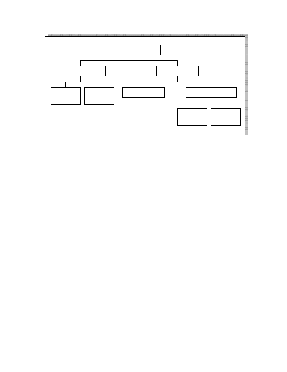
CR-Clean. Figure 2.1 shows that predator worms are
first classified according to their victim infection state
and then classified further according to their scanning
technique.
As shown in Figure 2.1, prey worms can be
patching or non-patching. Prey worms may protect
themselves from their predators by closing the security
hole through which they penetrated, thus preventing
predator from getting in. We call such prey worms a
patching worm otherwise they are non-patching prey
worms.
Worms that can attack an infected machine, wipe
the existing worm, and takeover that machine are
called predator worms, e.g. Code-Green, Welchi, and
Netsky. On the other hand, prey worms are the victims
of predator worms, e.g. MS-Blast, Bagle, and Sasser.
Figure 2.1 explains the classification. Internet worms
according to their predatory role.
2.2 Environment
We assume The Internet size is fixed during any
infection cycle. Thus, total number of machines
is
M
which is constant. Any machine can be either
susceptible to an infection by some worm (called
vulnerable) or immune (called removed). Vulnerable
machines can be penetrated by a worm, and once
infected they spread the infection on their own.
Removed machines cannot be infected by a worm for
Patching
Internet Worm
Prey Worm
Predator Worm
Infection-Driven
Vulnerability-Driven
Non-
Patching
Active-
Spreading
Passive-
Spreading
Figure 2.1. Worm Classification. Worms can be classified
according to their predatory characteristics, e.g. their spread
trigger and scanning technique.
Published in the IIU/IEEE Proc. of International Conference on Computer & Communication Engineering,
ICCCE '06, Kuala Lumpur, Malaysia, May 2006, Vol-I, Page 157-163.
159
some reason; e.g. the worm doesn't run on that
machine's platform or the machine doesn't have the
related security flaw. If the number of vulnerable
machines is
S
, and number of immune machines is
R
, then
M
R
S
=
+
is the total number of machines.
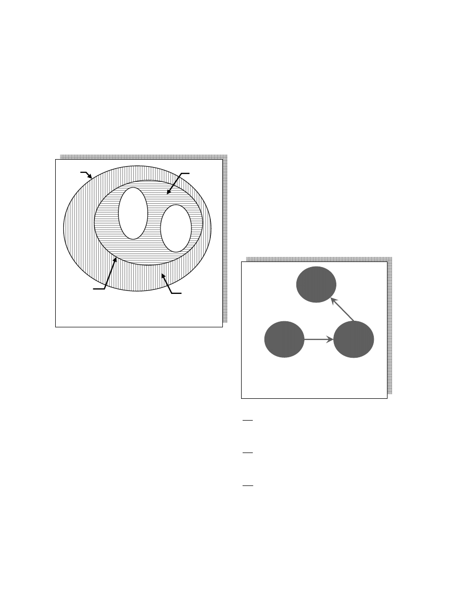
Figure 2.2 shows the two main sets set-S and set-R.
Usually, vulnerable and removed machines don’t
switch back and forth. However, in some cases a
vulnerable machine may become immune; e.g. when
and operating system patch is applied such that the
related security flaw is fixed.
A vulnerable machine that is infected by a worm is
called infectious. All other vulnerable machines that
are not compromised are in the clean machines set (set-
n) of size
)
(t
n
. Machines can change their state from
clean to infectious, or infectious to clean. We assume
that an infectious machine is infected by only one of
two worms: a prey or a predator worm. Infectious
machines that are infected by a prey worm (worm-x)
are called set-x, which has cardinality of
)
(t
x
.
Machines that are infected by predator worm (worm-y)
form set-y with of size
)
(t
y
. Figure 2.2 shows the two
infectious sets and their relation to the clean set.
Machines in set-x can change state and move into set-
y. The cardinalities of set-n, set-x, and set-y, are
variable functions of time, where the total sum
)
(
)
(
)
(
t
y
t
x
t
n
S
+
+
=
is the size of vulnerable
machines set.
3. Scenario-1: Prey, Predator Model
In the basic scenario, two combating worms (a prey
and a predator) spread over a network. Worm-x is a
traditional prey worm, which spreads by infecting
clean machines.
Worm-y is infection-driven predator
worm that can spread only by taking over machines
infected by worm-x. The size of worm-x population at
anytime is
)
(t
x
while size of worm-y population is
)
(t
y
. Figure 3.1 describes the interaction between the
different sets in this scenario. Directed links signifies
the transition rate of members between two sets.
Set-x size increases at rate proportional to both the
size of set-x and set-n. In other words, at anytime the
increase in the number of machines infected by worm-
x depends on the number of already worm-x machines
and the number of existing clean machines. On the
other hand, any encounter between worm-x and worm-
y instances will result in an increase in worm-y
population on count of worm-x population. Thus, set-y
size increase at rate proportional to the number of
worm-x and worm-y infected machines.
The infection rate of worm-x is the first derivative
of
)
(t
x
. The same applies to worm-y and clean
machines change rate. The dynamic of the system are
described by equations 3.1, 3.2, 3.3, and 3.4.
bxy
axn
dt
dx
−
=
(3.1)
bxy
dt
dy =
(3.2)
axn
dt
dn
−
=
(3.3)
0
0
0
)
0
(
,
)
0
(
,
)
0
(
n
n
y
y
x
x
=
=
=
(3.4)
set-y
y(t)
set-n
s(t)
set-x
x(t)
set-S
S
set-R
R
M
Figure 2.2 Machine Sets
Figure 3.1. Transition between the prey and
infection-driven predator worms. The circles
indicate machines' sets, while arrows indicate
transitions' direction and rate.
set-y
y(t)
axn
set-n
n(t)
bxy
set-x
x(t)
Published in the IIU/IEEE Proc. of International Conference on Computer & Communication Engineering,
ICCCE '06, Kuala Lumpur, Malaysia, May 2006, Vol-I, Page 157-163.
160
Both
a
and
b
are positive parameters that depend
on worms' scanning rate and network size. Below, we
discuss the derivation of
a
and
b
values.
3.1 Parameters Derivation
Let worm-x scanning rate be
r
, where
r
is the
number of unique scans generated by the worm per a
unit of time. Thus, the total number of scans by all
members in set-x is
rx
. Since R+x(t)+y(t)+n(t)=M,
the value of
rx
is the sum of all scans by worm-x of
all machine sets, as in equation 3.5
M
rxn
rxy
rx
rxR
rx
+
+
+
=
2
(3.5)
If each time that worm-x scans a clean machine
results in a new infection, then parameter
a
is given
by equation 3.6
M
r
a
=
(3.6)
Likewise, if every encounter between y-worm and
worm-x infected machine results in a takeover by
worm-y, then parameter
b
is given by equation 3.7
M
r
b
=
(3.7)
The previous discussion applies to passive-
spreading predator. On the other hand, an active-
spreading predator does its own scanning in order to
find worm-x infected machines. If we assume that
worm-y has scanning rate be
v
, the total number of
scanning by members in set-y is
vy
satisfies equation
3.8
M
vyn
vy
vyx
vyR
vy
+
+
+
=
2
(3.8)
Since encounters between worm-x and worm-y
result from both scans by worm-x and worm-y. The
parameter
b
can be described by equation 3.9
M
r
v
b
+
=
(3.9)
3.2 Analysis
We used numerical solution to solve the equation
system described in 3.1, 3.2, 3.3, and 3.4. We used
Maple to draw the curves in figure 3.2 and 3.3.
Multiple curves in red for
)
(
t
x
and in green for
)
(
t
y
are plotted for different values of
b
a
:
.
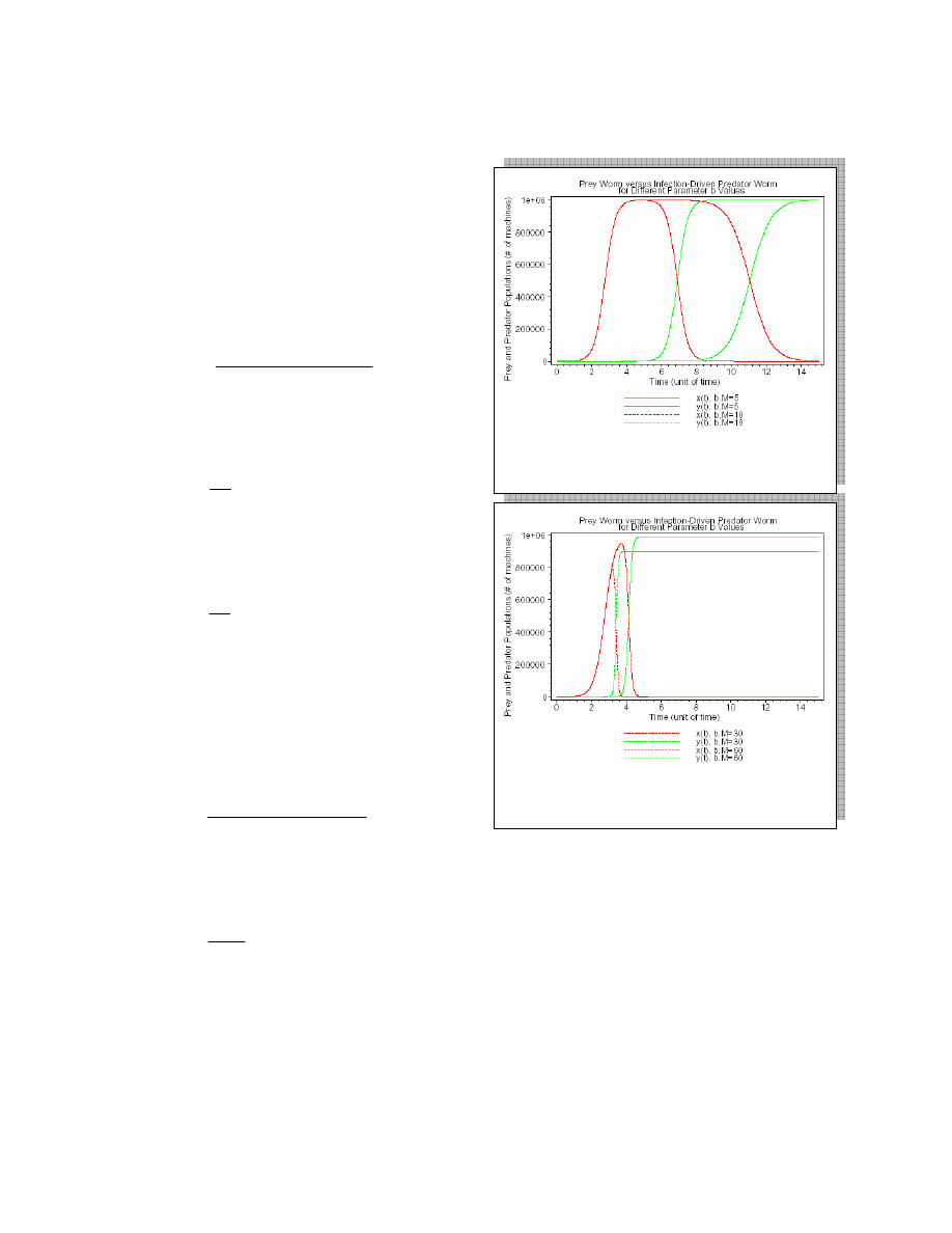
The general behavior described here shows that
initially worm-x increase exponentially as it would
without worm-y existence. Worm-y increase
proportional to increase in worm-x populations. The
increase in worm-y population results in decrease in
worm-x population, as worm-y takeover worm-x
machines. The
)
(
t
x
curve reaches its maximum when
it infects all vulnerable machines (figure 3.2) or when
worm-y is large enough to consume more worm-x
machines than can worm-x reproduce (figure 3.3).
Curve
)
(t
y
continues to increase until it uses up all
available worm-x members, where it hits its maximum
and freeze thereafter. The system reaches steady state
when both infection rates are zero. This occurs when
Figure 3.3. a.M=10, M=3000000, x0=100,
y0=1, n0=1000000.
Figure 3.2
. a.M=10, M=3000000, x0=100, y0=1,
n0=1000000.
Published in the IIU/IEEE Proc. of International Conference on Computer & Communication Engineering,
ICCCE '06, Kuala Lumpur, Malaysia, May 2006, Vol-I, Page 157-163.
161
all worm-x infected machines are re-infected by worm-
y (
)
(t
x
is zero).
In figure 3.2
S
y
x
=
=
)
max(
)
max(
. In other
words the maximum value of the curves is size of
vulnerable population. We name this condition as
Prey-outbreak condition since it occurs as result of
faster growth in prey population than predator
population (
a
b
≤
)
In figure 3.3
)
max(
)
max(
y
x
≤
. This condition
is called prey-cutback condition, which occurs when
the predator population is growing faster than the prey
(
a
b
>
).
4. Scenario-2: Prey, Vulnerability-Driven
Predator Model
We expand the basic by considering vulnerability-
driven type of predator, where worm-y can infect both
clean and worm-x infected machines. Figure 4.1
describes the transitions between the machines sets.
Worm-x increases as in the basic scenario. However,
worm-y increases by targeting clean machines at rate
cyn
(
c
is positive) in addition to infecting worm-x
machines. The system dynamics can be described in
equations 4.1, 4.2, 4.3, and 4.4.
bxy
axn
dt
dx
−
=
(4.1)
bxy
cyn
dt
dy
+
=
(4.2)
cyn
axn
dt
dn
−
−
=
(4.3)
0
0
0
)
0
(
,
)
0
(
,
)
0
(
n
n
y
y
x
x
=
=
=
(4.4)
Parameter
a
and
b
values are as derived in
previous section. The value of
c
which depends on
both worm-y scanning rate and network size is given in
equation 4.5
M
v
c
=
(4.5)
In case of vulnerability-driven predator (
0
>
c
) the
predator has more than one way to spread and thus isn't
totally dependent on the prey population. Any increase
in prey population will increase the predator population
and increasing the predator population will decrease
prey population. However, a decrease in the prey
population will not lead to a decrease in the predator's
population.
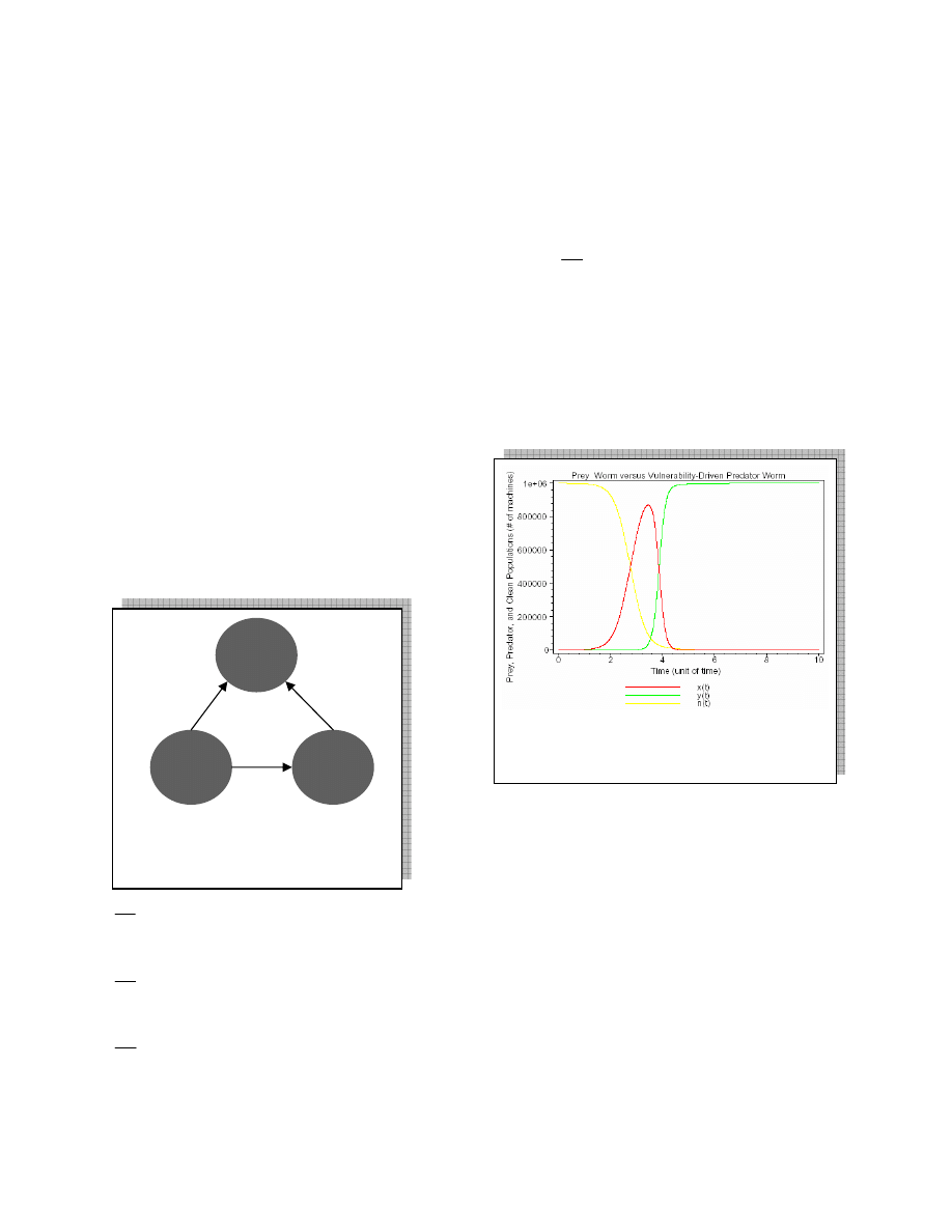
Figure 4.2 shows the plot of
)
(
t
n
,
)
(
t
x
and
)
(
t
y
.
Compared with figure 3.2 and 3.3, the behavior is
similar with two exceptions. First the prey-outbreak
condition doesn't happen. On the other hand
)
(
t
y
reaches the maximum of environment capacity, which
we call predator-outbreak condition. The figure shows
that prey-cutback condition will occur.
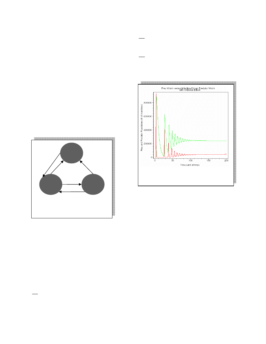
5. Scenario-3: Prey, Predator, and
Antivirus Model
Worm-x and worm-y are prey and predator worms
that are competing over an environment. Worm-y is
vulnerability-driven predator. Some machines on the
network run antivirus software that can detect and
clean both worms’ infections. This scenario is
Figure 4.2
. a.M=10, b.M=25, c.M=5,
M=3000000, x
0
=100, y
0
=1, n
0
=1000000.
Figure 4.1. Transition between prey and
vulnerability-driven predator worms. The
circles represent machine sets, while arrows
indicate transitions’ between them.
set-y
y(t)
axn
set-n
n(t)
bxy
set-x
x(t)
cyn
Published in the IIU/IEEE Proc. of International Conference on Computer & Communication Engineering,
ICCCE '06, Kuala Lumpur, Malaysia, May 2006, Vol-I, Page 157-163.
162
analogous to harvesting (spraying, or fishing)
phenomena in biological systems, where some third-
party eliminates members of both combating
populations. We assume that as people become aware
of an epidemic, they start to install or update antivirus
software at increasing rate.
We assume that the number of machines with
antivirus update to be an increasing function of time.
The functions
)
(
t
z
x
and
)
(t
z
y
are the fraction of
worm-x and worm-y infected machines, respectively,
that are cleaned by the antivirus software at anytime.
We define
)
(t
z
x
and
)
(t
z
y
in equations 4.1 and 4.2.
The constants
x
d
and
y
d
are fraction numbers that
determines the antivirus effectivenessy.
)
1
/(
)
(
+
=
t
t
d
t
z
y
y
(5.1)
)
1
/(
)
(
+
=
t
t
d
t
z
x
x
(5.2)
Figure 5.1 describes the transition of members
between machines’ sets as a result of the two worms
and antivirus reactions. Worm-x increase on count of
clean machines set (set-n) at rate
axn
. Meanwhile,
set-n gains worm-x machines back at rate
x
xz
, once
cleaned by the an antivirus. On the other hand, worm-y
increase on count of both clean and worm-x machines
at rate
bxy
cyn
+
. In contrary of all previous
scenarios, set-y decreases at rate
)
(t
yz
y
, as result of
antivirus effect. The system behavior is described by
equations 5.3, 5.4, 5.5, and 5.6
x
xz
bxy
axn
dt
dx
−
−
=
(5.3)
y
yz
bxy
cyn
dt
dy
−
+
=
(5.4)
y
x
yz
xz
cyn
axn
dt
dn
+
+
−
−
=
(5.5)
0
0
0
)
0
(
,
)
0
(
,
)
0
(
n
n
y
y
x
x
=
=
=
(5.6)
Figure 5.2 shows a new type of behavior, both
curves
)
(t
x
and
)
(t
y
oscillate for a while as they
gradually become constant lines. This phenomenon is a
result of introducing the antivirus effect, which kills
predators as will as prey infections. Originally, the
increase in predators population causes degrade in prey
population, and this is what is initially happening in
this case. However, as the antivirus cleans some
predator infections causing its population to drop, more
prey infections will have chance to survive, and thus
prey population increases again. Increasing prey
population results in increasing predator population.
However the second peek is lower than the first once
since the antivirus is continuously reducing both
populations. This periodical behavior repeats itself
each time with lower maximum values. The oscillation
turns into straight lines with some vibration, which
eventually diminishes, resulting into two constant
lines. At this stage the system reaches its steady state
or equilibrium point.
6. Conclusion & Future Work
Figure 5.2. c.M=0, a.M=10, b.M=25,
d
x
=d
y
=0.07, x
0
=100, y0=1, n
0
=1000000,
M=3000000.
Figure 5.1. Inter-set transition for scenario-
2. The circles are sets. While arrows are
transitions’ direction and their rate.
set-y
y(t)
axn
set-n
n(t)
bxy
set-x
x(t)
cyn
xz
x
yz
y

Published in the IIU/IEEE Proc. of International Conference on Computer & Communication Engineering,
ICCCE '06, Kuala Lumpur, Malaysia, May 2006, Vol-I, Page 157-163.
163
In this paper we have presented several scenarios of
virus-virus warfare. We classify worm types according
to their predatory characteristics. We study and analyze
the prey and predator interaction, and investigate the
related parameters' values. We study several advanced
scenarios, including antivirus effect on prey-predator
system. Since the beginning of this work co-
incidentally several ware-fare has been reported in real
Internet. However, we must warn this work does not
model the specific warfare.
There are actually additional scenarios which can be
potentially modeled. One example is Cascade Chain
Worms (Wave Worm). Many worms have more than
one version. The new versions are meant to update the
old ones. However, existence of old versions can have
positive or negative effect of the spread of the new
version. Our current model considers the number
infected machines to be the worm population size. This
is true as long as each machine has only single
infection. In the future we will extend our work to
study the Multi-Infection machine scenario. Up to
date, all existing models, including those in this paper,
are based on random network model. In reality, the
Internet is a scale-free network [9], which can help in
the spread of worms’ vaccines [8].
7. References
[1]
H. Toyoizumi, A. Kara. Predators: Good Will Mobile
Codes Combat against Computer Viruses. Proc. of the
2002 New Security Paradigms Workshop, 2002
[2]
T.A. Burton. Volterra Integral and Differential
Equations. New York: Academic Press, 1983
[3]
S. Staniford, V. Paxson, N. Weaver. How to 0wn the
Internet in Your Spare Time. In Proc. of the 11
th
USENIX Security Symposium, 2002.
[4]
D. Nicol, M. Lilijenstam. Models of Active Worm
Defenses. IPSI, 2004
[5]
S. Staniford. Analysis of Spread of July Infestation of
the Code Red Worm.
http://www.silicondefense.com/cr/july.html
, 2001
[6]
C. Zou, W. Gong, D. Towsley. Code Red Worm
Propagation Modeling and Analysis, CCS, 2002
[7]
D. Moore. Network Telescopes: Observing Small or
Distant Security Events. Invited presentation at the 11
th
USENIX Security Symposium (Security ’02), 2002
[8]
J. Balthrop, S. Forrest, M. Newman, M. Williamson.
Technological Networks and the Spread of Computer
Viruses. Science Magazine, Vol 304, Pag 527-9, 2004
[9]
R. Albert, H. Jeong, A. Barabàsi. Internet: Diameter of
the World-Wide Web, Nature, Vol 401, Pag 130-1,
1999
Wyszukiwarka
Podobne podstrony:
więcej podobnych podstron