
Reduction Theory and the Lagrange–Routh Equations
Jerrold E. Marsden
∗
Control and Dynamical Systems 107-81
California Institute of Technology
Pasadena CA 91125, USA
marsden@cds.caltech.edu
Tudor S. Ratiu
†
D´epartement de Math´ematiques
´
Ecole Polyt´echnique F´ed´erale de Lausanne
CH - 1015 Lausanne Switzerland
Tudor.Ratiu@epfl.ch
J¨
urgen Scheurle
Zentrum Mathematik
TU M¨
unchen, Arcisstrasse 21
D-80290 M¨
unchen Germany
scheurle@mathematik.tu-muenchen.de
July, 1999: this version April 18, 2000
Abstract
Reduction theory for mechanical systems with symmetry has its roots in the clas-
sical works in mechanics of Euler, Jacobi, Lagrange, Hamilton, Routh, Poincar´
e and
others. The modern vision of mechanics includes, besides the traditional mechanics
of particles and rigid bodies, field theories such as electromagnetism, fluid mechanics,
plasma physics, solid mechanics as well as quantum mechanics, and relativistic theories,
including gravity.
Symmetries in these theories vary from obvious translational and rotational sym-
metries to less obvious particle relabeling symmetries in fluids and plasmas, to subtle
symmetries underlying integrable systems. Reduction theory concerns the removal of
symmetries and their associated conservation laws. Variational principles along with
symplectic and Poisson geometry, provide fundamental tools for this endeavor. Re-
duction theory has been extremely useful in a wide variety of areas, from a deeper
understanding of many physical theories, including new variational and Poisson struc-
tures, stability theory, integrable systems, as well as geometric phases.
This paper surveys progress in selected topics in reduction theory, especially those
of the last few decades as well as presenting new results on nonabelian Routh reduction.
We develop the geometry of the associated Lagrange–Routh equations in some detail.
The paper puts the new results in the general context of reduction theory and discusses
some future directions.
∗
Research partially supported by the National Science Foundation, the Humboldt Foundation, and the
California Institute of Technology
†
Research partially supported by the US and Swiss National Science Foundations and the Humboldt
Foundation
1

CONTENTS
2
Contents
3
Overview . . . . . . . . . . . . . . . . . . . . . . . . . . . . . . . . . . . . . .
3
Bundles, Momentum Maps, and Lagrangians . . . . . . . . . . . . . . . . . .
7
Coordinate Formulas . . . . . . . . . . . . . . . . . . . . . . . . . . . . . . . .
8
. . . . . . . . . . . . . . . . . . . . . . . . . . . . . . .
9
e Reduction . . . . . . . . . . . . . . . . . . . . . . . . . . . . . 10
Lie–Poisson Reduction . . . . . . . . . . . . . . . . . . . . . . . . . . . . . . . 11
Examples . . . . . . . . . . . . . . . . . . . . . . . . . . . . . . . . . . . . . . 13
2 The Bundle Picture in Mechanics
18
Cotangent Bundle Reduction . . . . . . . . . . . . . . . . . . . . . . . . . . . 18
Lagrange-Poincar´e Reduction . . . . . . . . . . . . . . . . . . . . . . . . . . . 19
Hamiltonian Semidirect Product Theory . . . . . . . . . . . . . . . . . . . . . 20
Semidirect Product Reduction by Stages . . . . . . . . . . . . . . . . . . . . . 22
Lagrangian Semidirect Product Theory
. . . . . . . . . . . . . . . . . . . . . 22
Reduction by Stages . . . . . . . . . . . . . . . . . . . . . . . . . . . . . . . . 25
26
The Global Realization Theorem for the Reduced Phase Space . . . . . . . . 27
The Routhian. . . . . . . . . . . . . . . . . . . . . . . . . . . . . . . . . . . . 29
Examples . . . . . . . . . . . . . . . . . . . . . . . . . . . . . . . . . . . . . . 30
Hamilton’s Variational Principle and the Routhian . . . . . . . . . . . . . . . 30
The Routh Variational Principle on Quotients . . . . . . . . . . . . . . . . . . 33
Curvature . . . . . . . . . . . . . . . . . . . . . . . . . . . . . . . . . . . . . . 35
Splitting the Reduced Variational Principle . . . . . . . . . . . . . . . . . . . 38
The Lagrange–Routh Equations . . . . . . . . . . . . . . . . . . . . . . . . . . 39
Examples . . . . . . . . . . . . . . . . . . . . . . . . . . . . . . . . . . . . . . 41
42
. . . . . . . . . . . . . . . . . . . . . . . . . . 42
Second Reconstruction Equation . . . . . . . . . . . . . . . . . . . . . . . . . 43
Third Reconstruction Equation . . . . . . . . . . . . . . . . . . . . . . . . . . 44
The Vertical Killing Metric . . . . . . . . . . . . . . . . . . . . . . . . . . . . 45
Fourth Reconstruction Equation . . . . . . . . . . . . . . . . . . . . . . . . . 47
Geometric Phases . . . . . . . . . . . . . . . . . . . . . . . . . . . . . . . . . . 48
5 Future Directions and Open Questions
49
1 Introduction
3
1
Introduction
This section surveys some of the literature and basic results in reduction theory. We will
come back to many of these topics in ensuing sections.
1.1
Overview
A Brief History of Reduction Theory.
We begin with an overview of progress in
reduction theory and some new results in Lagrangian reduction theory. Reduction theory,
which has its origins in the classical work of Euler, Lagrange, Hamilton, Jacobi, Routh and
Poincar´e, is one of the fundamental tools in the study of mechanical systems with symmetry.
At the time of this classical work, traditional variational principles and Poisson brackets were
fairly well understood. In addition, several classical cases of reduction (using conservation
laws and/or symmetry to create smaller dimensional phase spaces), such as the elimination
of cyclic variables as well as Jacobi’s elimination of the node in the n-body problem, were
developed. The ways in which reduction theory has been generalized and applied since that
time has been rather impressive. General references in this area are Abraham and Marsden
[1978], Arnold [1989], and Marsden [1992].
Of the above classical works, Routh [1860, 1884] pioneered reduction for Abelian groups.
Lie [1890], discovered many of the basic structures in symplectic and Poisson geometry and
their link with symmetry. Meanwhile, Poincare [1901] discovered the generalization of the
Euler equations for rigid body mechanics and fluids to general Lie algebras. This was more
or less known to Lagrange [1788] for SO(3), as we shall explain in the body of the paper.
The modern era of reduction theory began with the fundamental papers of Arnold [1966a]
and Smale [1970]. Arnold focussed on systems on Lie algebras and their duals, as in the
works of Lie and Poincar´
e, while Smale focussed on the Abelian case giving, in effect, a
modern version of Routh reduction.
With hindsight we now know that the description of many physical systems such as
rigid bodies and fluids requires noncanonical Poisson brackets and constrained variational
principles of the sort studied by Lie and Poincar´
e. An example of a noncanonical Poisson
bracket on g
∗
, the dual of a Lie algebra g, is called, following Marsden and Weinstein [1983],
the Lie–Poisson bracket. These structures were known to Lie around 1890, although Lie
seemingly did not recognize their importance in mechanics. The symplectic leaves in these
structures, namely the coadjoint orbit symplectic structures, although implicit in Lie’s work,
were discovered by Kirillov, Kostant, and Souriau in the 1960’s.
To synthesize the Lie algebra reduction methods of Arnold [1966a] with the techniques
of Smale [1970] on the reduction of cotangent bundles by Abelian groups, Marsden and
Weinstein [1974] developed reduction theory in the general context of symplectic manifolds
and equivariant momentum maps; related results, but with a different motivation and con-
struction (not stressing equivariant momentum maps) were found by Meyer [1973].
The construction is now standard: let (P, Ω) be a symplectic manifold and let a Lie
group G act freely and properly on P by symplectic maps. The free and proper assumption
is to avoid singularities in the reduction procedure as is discussed later. Assume that this
action has an equivariant momentum map J : P
→ g
∗
. Then the symplectic reduced
space J
−1
(µ)/G
µ
= P
µ
is a symplectic manifold in a natural way; the induced symplectic
form Ω
µ
is determined uniquely by π
∗
µ
Ω
µ
= i
∗
µ
Ω where π
µ
: J
−1
(µ)
→ P
µ
is the projection
and i
→ P is the inclusion. If the momentum map is not equivariant, Souriau
[1970] discovered how to centrally extend the group (or algebra) to make it equivariant.
Coadjoint orbits were shown to be symplectic reduced spaces by Marsden and Weinstein
[1974]. In the reduction construction, if one chooses P = T
∗
G, with G acting by (say left)
translation, the corresponding space P
µ
is identified with the coadjoint orbit
O
µ
through
1.1 Overview
4
µ together with its coadjoint orbit symplectic structure. Likewise, the Lie–Poisson bracket
on g
∗
is inherited from the canonical Poisson structure on T
∗
G by Poisson reduction, that
is, by simply identifying g
∗
with the quotient (T
∗
G)/G. It is not clear who first explicitly
observed this, but it is implicit in many works such as Lie [1890], Kirillov [1962, 1976],
Guillemin and Sternberg [1980], and Marsden and Weinstein [1982, 1983], but is explicit in
Marsden, Weinstein, Ratiu and Schmid [1983], and in Holmes and Marsden [1983].
Kazhdan, Kostant and Sternberg [1978] showed that P
µ
is symplectically diffeomorphic
to an orbit reduced space P
µ
∼
= J
−1
(
O
µ
)/G and from this it follows that P
µ
are the sym-
plectic leaves in P/G. This paper was also one of the first to notice deep links between
reduction and integrable systems, a subject continued by, for example, Bobenko, Reyman
and Semenov-Tian-Shansky [1989] in their spectacular group theoretic explanation of the
integrability of the Kowalewski top.
The way in which the Poisson structure on P
µ
is related to that on P/G was clarified in
a generalization of Poisson reduction due to Marsden and Ratiu [1986], a technique that has
also proven useful in integrable systems (see, e.g., Pedroni [1995] and Vanhaecke [1996]).
Reduction theory for mechanical systems with symmetry has proven to be a power-
ful tool enabling advances in stability theory (from the Arnold method to the energy-
momentum method) as well as in bifurcation theory of mechanical systems, geometric phases
via reconstruction—the inverse of reduction—as well as uses in control theory from stabi-
lization results to a deeper understanding of locomotion. For a general introduction to some
of these ideas and for further references, see Marsden and Ratiu [1999].
More About Lagrangian Reduction.
Routh reduction for Lagrangian systems is classi-
cally associated with systems having cyclic variables (this is almost synonymous with having
an Abelian symmetry group); modern accounts can be found in Arnold [1988]Arnold, Ko-
zlov and Neishtadt [1988] and in Marsden and Ratiu [1999],
§8.9. A key feature of Routh
reduction is that when one drops the Euler–Lagrange equations to the quotient space asso-
ciated with the symmetry, and when the momentum map is constrained to a specified value
(i.e., when the cyclic variables and their velocities are eliminated using the given value of
the momentum), then the resulting equations are in Euler–Lagrange form not with respect
to the Lagrangian itself, but with respect to the Routhian. In his classical work, Routh
[1877] applied these ideas to stability theory, a precursor to the energy-momentum method
for stability (Simo, Lewis and Marsden [1991]; see Marsden [1992] for an exposition and
references). Of course, Routh’s stability method is still widely used in mechanics.
Another key ingredient in Lagrangian reduction is the classical work of Poincare [1901]
in which the Euler–Poincar´
e equations were introduced. Poincar´e realized that both the
equations of fluid mechanics and the rigid body and heavy top equations could all be de-
scribed in Lie algebraic terms in a beautiful way. The imporance of these equations was
realized by Hamel [1904, 1949] and Chetayev [1941].
Tangent and Cotangent Bundle Reduction.
The simplest case of cotangent bundle
reduction is reduction at zero in which case one chooses P = T
∗
Q and then the reduced
space at µ = 0 is given by P
0
= T
∗
(Q/G), the latter with the canonical symplectic form.
Another basic case is when G is Abelian. Here, (T
∗
Q)
µ
∼
= T
∗
(Q/G) but the latter has a
symplectic structure modified by magnetic terms; that is, by the curvature of the mechanical
connection.
The Abelian version of cotangent bundle reduction was developed by Smale [1970] and
Satzer [1977] and was generalized to the nonabelian case in Abraham and Marsden [1978].
Kummer [1981] introduced the interpretations of these results in terms of a connection, now
called the mechanical connection. The geometry of this situation was used to great effect
1.1 Overview
5
in, for example, Guichardet [1984], Iwai [1987c, 1990], and Montgomery [1984, 1990, 1991a].
Routh reduction may be viewed as the Lagrangian analogue of cotangent bundle reduction.
Tangent and cotangent bundle reduction evolved into what we now term as the “bundle
picture” or the “gauge theory of mechanics”. This picture was first developed by Mont-
gomery, Marsden and Ratiu [1984] and Montgomery [1984, 1986]. That work was moti-
vated and influenced by the work of Sternberg [1977] and Weinstein [1978] on a Yang-Mills
construction that is, in turn, motivated by Wong’s equations, that is, the equations for a
particle moving in a Yang-Mills field. The main result of the bundle picture gives a structure
to the quotient spaces (T
∗
Q)/G and (T Q)/G when G acts by the cotangent and tangent
lifted actions. We shall review this structure in some detail in the body of the paper.
Marsden and Scheurle [1993a,b] showed how to gener-
alize the Routh theory to the nonabelian case as well as realizing how to get the Euler–
Poincar´e equations for matrix groups by the important technique of reducing variational
principles. This approach was motivated by related earlier work of Cendra and Marsden
[1987] and Cendra, Ibort and Marsden [1987]. The work of Bloch, Krishnaprasad, Marsden
and Ratiu [1996] generalized the Euler–Poincar´
e variational structure to general Lie groups
and Cendra, Marsden and Ratiu [2000a] carried out a Lagrangian reduction theory that
extends the Euler–Poincar´
e case to arbitrary configuration manifolds. This work was in the
context of the Lagrangian analogue of Poisson reduction in the sense that no momentum
map constraint is imposed.
One of the things that makes the Lagrangian side of the reduction story interesting
is the lack of a general category that is the Lagrangian analogue of Poisson manifolds.
Such a category, that of Lagrange-Poincar´
e bundles, is developed in Cendra, Marsden and
Ratiu [2000a], with the tangent bundle of a configuration manifold and a Lie algebra as
its most basic example. That work also develops the Lagrangian analogue of reduction
for central extensions and, as in the case of symplectic reduction by stages (see Marsden,
Misiolek, Perlmutter and Ratiu [1998, 2000]), cocycles and curvatures enter in this context
in a natural way.
The Lagrangian analogue of the bundle picture is the bundle (T Q)/G, which, as shown
later, is a vector bundle over Q/G; this bundle was studied in Cendra, Marsden and Ratiu
[2000a]. In particular, the equations and variational principles are developed on this space.
For Q = G this reduces to Euler–Poincar´e reduction and for G Abelian, it reduces to the
classical Routh procedure. Given a G-invariant Lagrangian L on T Q, it induces a Lagrangian
l on (T Q)/G. The resulting equations inherited on this space, given explicitly later, are the
Lagrange–Poincar´
e equations (or the reduced Euler–Lagrange equations).
Methods of Lagrangian reduction have proven very useful in, for example, optimal control
problems. It was used in Koon and Marsden [1997a] to extend the falling cat theorem of
Montgomery [1990] to the case of nonholonomic systems as well as non-zero values of the
momentum map.
Semidirect Product Reduction.
Recall that in the simplest case of a semidirect prod-
uct, one has a Lie group G that acts on a vector space V (and hence on its dual V
∗
) and then
one forms the semidirect product S = G
V , generalizing the semidirect product structure
of the Euclidean group SE(3) = SO(3)
R
3
.
Consider the isotropy group G
a
0
for some a
0
∈ V
∗
. The semidirect product reduction
theorem states that each of the symplectic reduced spaces for the action of G
a
0
on T
∗
G
is symplectically diffeomorphic to a coadjoint orbit in (g
V )
∗
, the dual of the Lie algebra
of the semi-direct product. This semidirect product theory was developed by Guillemin
and Sternberg [1978, 1980], Ratiu [1980a, 1981, 1982], and Marsden, Ratiu and Weinstein
[1984a,b].
1.1 Overview
6
This construction is used in applications where one has “advected quantities” (such as
the direction of gravity in the heavy top, density in compressible flow and the magnetic
field in MHD). Its Lagrangian counterpart was developed in Holm, Marsden and Ratiu
[1998b] along with applications to continuum mechanics. Cendra, Holm, Hoyle and Marsden
[1998] applied this idea to the Maxwell–Vlasov equations of plasma physics. Cendra, Holm,
Marsden and Ratiu [1998] showed how Lagrangian semidirect product theory it fits into the
general framework of Lagrangian reduction.
Reduction by Stages and Group Extensions.
The semidirect product reduction the-
orem can be viewed using reduction by stages: if one reduces T
∗
S by the action of the
semidirect product group S = G
V in two stages, first by the action of V at a point a
0
and then by the action of G
a
0
. Semidirect product reduction by stages for actions of semidi-
rect products on general symplectic manifolds was developed and applied to underwater
vehicle dynamics in Leonard and Marsden [1997]. Motivated partly by semidirect product
reduction, Marsden, Misiolek, Perlmutter and Ratiu [1998, 2000] gave a significant general-
ization of semidirect product theory in which one has a group M with a normal subgroup
N
⊂ M (so M is a group extension of N) and M acts on a symplectic manifold P . One
wants to reduce P in two stages, first by N and then by M/N . On the Poisson level this is
easy: P/M ∼
= (P/N )/(M/N ), but on the symplectic level it is quite subtle.
Cotangent bundle reduction by stages is especially interesting for group extensions. An
example of such a group, besides semidirect products, is the Bott-Virasoro group, where the
Gelfand-Fuchs cocycle may be interpreted as the curvature of a mechanical connection. The
work of Cendra, Marsden and Ratiu [2000a] briefly described above, contains a Lagrangian
analogue of reduction for group extensions and reduction by stages.
Singular Reduction.
Singular reduction starts with the observation of Smale [1970] that
z
∈ P is a regular point of J iff z has no continuous isotropy. Motivated by this, Arms,
Marsden and Moncrief [1981, 1982] showed that the level sets J
−1
(0) of an equivariant
momentum map J have quadratic singularities at points with continuous symmetry. While
such a result is easy for compact group actions on finite dimensional manifolds, the main
examples of Arms, Marsden and Moncrief [1981] were, in fact, infinite dimensional—both
the phase space and the group. Otto [1987] has shown that if G is a compact Lie group,
J
−1
(0)/G is an orbifold. Singular reduction is closely related to convexity properties of the
momentum map (see Guillemin and Sternberg [1982], for example).
The detailed structure of J
−1
(0)/G for compact Lie groups acting on finite dimensional
manifolds was developed in Sjamaar and Lerman [1991] and extended for proper Lie group
actions to J
)/G by Bates and Lerman [1997], if
. Ortega
[1998] and Ortega and Ratiu [2001] redid the entire singular reduction theory for proper
Lie group actions starting with the point reduced spaces J
−1
(µ)/G
µ
and also connected it
to the more algebraic approach to reduction theory of Arms, Cushman and Gotay [1991].
Specific examples of singular reduction and further references may be found in Cushman
and Bates [1997]. This theory is still under development.
The Method of Invariants.
This method seeks to parameterize quotient spaces by group
invariant functions. It has a rich history going back to Hilbert’s invariant theory. It has
been of great use in bifurcation with symmetry (see Golubitsky, Stewart and Schaeffer [1988]
for instance). In mechanics, the method was developed by Kummer, Cushman, Rod and
coworkers in the 1980’s. We will not attempt to give a literature survey here, other than
to refer to Kummer [1990], Kirk, Marsden and Silber [1996], Alber, Luther, Marsden and
Robbins [1998] and the book of Cushman and Bates [1997] for more details and references.
1.2 Bundles, Momentum Maps, and Lagrangians
7
The New Results in this Paper.
The main new results of the present paper are:
1. In
§3.1, a global realization of the reduced tangent bundle, with a momentum map
constraint, in terms of a fiber product bundle, which is shown to also be globally
diffeomorphic to an associated coadjoint orbit bundle.
2.
§3.5 shows how to drop Hamilton’s variational principle to these quotient spaces
3. We derive, in
§3.8, the corresponding reduced equations, which we call the Lagrange–
Routh equations, in an intrinsic and global fashion.
4. In
§4 we give a Lagrangian view of some known and new reconstruction and geometric
phase formulas.
The Euler free rigid body, the heavy top, and the underwater vehicle are used to illustrate
some of the points of the theory. The main techniques used in this paper build primarily
on the work of Marsden and Scheurle [1993a,b] and of Jalnapurkar and Marsden [2000a] on
nonabelian Routh reduction theory, but with the recent developments in Cendra, Marsden
and Ratiu [2000a] in mind.
1.2
Bundles, Momentum Maps, and Lagrangians
The Shape Space Bundle and Lagrangian.
We shall be primarily concerned with the
following setting. Let Q be a configuration manifold and let G be a Lie group that acts
freely and properly on Q. The quotient Q/G =: S is referred to as the shape space and Q
is regarded as a principal fiber bundle over the base space S. Let π
Q,G
: Q
→ Q/G = S be
the canonical projection.
We call the map π
Q,G
: Q
→ Q/G the shape space bundle.
Let
·, · be a G-invariant metric on Q, also called a mass matrix. The kinetic energy
K : T Q
→ R is defined by K(v
q
) =
1
2
v
q
, v
q
. If V is a G-invariant potential on Q, then
the Lagrangian L = K
− V : T Q → R is also G-invariant. We focus on Lagrangians of this
form, although much of what we do can be generalized. We make a few remarks concerning
this in the body of the paper.
Momentum Map, Mechanical Connection, and Locked Inertia.
Let G have Lie
algebra g and J
L
: T Q
→ g
∗
be the momentum map on T Q, which is defined by J
L
(v
q
)
·ξ =
v
q
, ξ
Q
(q)
. Here v
q
∈ T
q
Q, ξ
∈ g, and ξ
Q
denotes the infinitesimal generator corresponding
to ξ.
Recall that a principal connection
A : T Q → g is an equivariant g-valued one form on
T Q that satisfies
A(ξ
Q
(q)) = ξ and its kernel at each point, denoted Hor
q
, complements the
vertical space, namely the tangents to the group orbits. Let A : T Q
→ g be the mechanical
connection, namely the principal connection whose horizontal spaces are orthogonal to
the group orbits.
For each q
∈ Q, the locked inertia tensor I(q) : g → g
∗
, is defined
by the equation
I(q)ξ, η = ξ
Q
(q), η
Q
(q)
. The locked inertia tensor has the following
equivariance property: I(g
· q) = Ad
∗
g
−1
I(q) Ad
g
−1
, where the adjoint action by a group
element g is denoted Ad
g
and Ad
∗
g
−1
denotes the dual of the linear map Ad
g
−1
: g
→ g. The
mechanical connection A and the momentum map J
L
are related as follows:
J
L
(v
q
) = I(q)A(v
q
)
i.e.,
A(v
q
) = I(q)
−1
J
L
(v
q
).
(1.1)
1
The theory of quotient manifolds guarantees (because the action is free and proper) that Q/G is a
smooth manifold and the map π
Q,G
is smooth. See Abraham, Marsden and Ratiu [1988] for the proof of
these statements.
2
[Shape space and its geometry also play an interesting and key role in computer vision. See for example,
1.3 Coordinate Formulas
8
In particular, or from the definitions, we have that J
L
(ξ
Q
(q)) = I(q)ξ. For free actions
and a Lagrangian of the form kinetic minus potential energy, the locked inertia tensor is
invertible at each q
∈ Q. Many of the constructions can be generalized to the case of regular
Lagrangians, where the locked inertia tensor is the second fiber derivative of L (see Lewis
[1992]).
Horizontal and Vertical Decomposition.
We use the mechanical connection A to
express v
q
(also denoted ˙q) as the sum of horizontal and vertical components:
v
q
= Hor(v
q
) + V er(v
q
) = Hor(v
q
) + ξ
Q
(q)
where ξ = A(v
q
). Thus, the kinetic energy is given by
K(v
q
) =
1
2
v
q
, v
q
=
1
2
Hor(v
q
), Hor(v
q
)
+
1
2
ξ
Q
(q), ξ
Q
(q)
Being G-invariant, the metric on Q induces a metric
· , ·
S
on S by
u
x
, v
x
S
=
u
q
, v
q
,
where u
q
, v
q
∈ T
q
Q are horizontal, π
Q,G
(q) = x and T π
Q,G
· u
q
= u
x
, T π
Q,G
· v
q
= v
x
.
Useful Formulas for Group Actions.
The following formulas are assembled for conve-
nience (see, for example, Marsden and Ratiu [1999] for the proofs). We denote the action
of g
∈ G on a point q ∈ Q by gq = g · q = Φ
g
(q), so that Φ
g
: Q
→ Q is a diffeomorphism.
1. Transformations of generators: T Φ
g
· ξ
Q
(q) = (Ad
g
ξ)
Q
(g
· q). which we also write,
using concatenation notation for actions, as g
· ξ
Q
(q) = (Ad
g
ξ)
Q
(g
· q).
2. Brackets of Generators: [ξ
Q
, η
Q
] =
−[ξ, η]
Q
3. Derivatives of Curves. Let q(t) be a curve in Q and let g(t) be a curve in G. Then
d
dt
(g(t)
· q(t)) =
Ad
g(t)
ξ(t)
Q
(g(t)
· q(t)) + g(t) · ˙q(t)
= g(t)
·
(ξ(t))
Q
(q(t)) + ˙q(t)
(1.2)
where ξ(t) = g(t)
−1
· ˙g(t).
It is useful to recall the Cartan formula. Let α be a one form and let X and Y be two
vector fields on a manifold. Then the exterior derivative dα of α is related to the Jacobi-Lie
bracket of vector fields by dα(X , Y ) = X[α(Y )]
− Y [α(X)] − α([X , Y ]).
1.3
Coordinate Formulas
We next give a few coordinate formulas for the case when G is Abelian.
The Coordinates and Lagrangian.
In a local trivialization, Q is realized as U
× G
where U is an open set in shape space S = Q/G. We can accordingly write coordinates
for Q as x
α
, θ
a
where x
α
, α = 1, . . . n are coordinates on S and where θ
a
, a = 1, . . . , r are
coordinates for G. In a local trivialization, θ
a
are chosen to be cyclic coordinates in the
classical sense. We write L (with the summation convention in force) as
L(x
α
, ˙x
β
, ˙θ
a
) =
1
2
g
αβ
˙x
α
˙x
β
+ g
αa
˙x
α
˙θ
a
+
1
2
g
ab
˙θ
a
˙θ
b
− V (x
α
).
(1.3)
The momentum conjugate to the cyclic variable θ
a
is J
a
= ∂L/∂ ˙θ
a
= g
αa
˙x
α
+ g
ab
˙θ
b
, which
are the components of the map J
L
.

1.4 VariationalPrinciples
9
Mechanical Connection and Locked Inertia Tensor.
The locked inertia tensor is the
matrix I
ab
= g
ab
and its inverse is denoted I
ab
= g
ab
. The matrix I
ab
is the block in the
matrix of the metric tensor g
ij
associated to the group variables and, of course, I
ab
need not
be the corresponding block in the inverse matrix g
ij
. The mechanical connection, as a vector
valued one form, is given by A
a
= dθ
a
+ A
a
α
dx
α
, where the components of the mechanical
connection are defined by A
b
α
= g
ab
g
aα
. Notice that the relation J
L
(v
q
) = I(q)
· A(v
q
) is
clear from this component formula.
Horizontal and Vertical Projections.
For a vector v = ( ˙x
α
, ˙θ
a
), and suppressing the
base point (x
α
, θ
a
) in the notation, its horizontal and vertical projections are verified to be
Hor(v) = ( ˙x
α
,
−g
ab
g
αb
˙x
α
)
and
Ver(v) = (0, ˙θ
a
+ g
ab
g
αb
˙x
α
).
Notice that v = Hor(v) + Ver(v), as it should.
Horizontal Metric.
In coordinates, the horizontal kinetic energy is
1
2
g(Hor(v), Hor(v)) =
1
2
g
αβ
˙x
α
˙x
β
− g
aα
g
ab
g
bβ
˙x
α
˙x
β
+
1
2
g
aα
g
ab
g
bβ
˙x
α
˙x
β
=
1
2
g
αβ
− g
aα
g
ab
g
bβ
˙x
α
˙x
β
(1.4)
Thus, the components of the horizontal metric (the metric on shape space) are given by
A
αβ
= g
αβ
− g
αd
g
da
g
βa
.
1.4
Variational Principles
Variations and the Action Functional.
Let q : [a, b]
→ Q be a curve and let δq =
d
dε
ε=0
q
ε
be a variation of q. Given a Lagrangian L, let the associated action functional
S
L
(q
ε
) be defined on the space of curves in Q defined on a fixed interval [a, b] by
S
L
(q
ε
) =
b
a
L(q
ε
, ˙q
ε
) dt .
The differential of the action function is given by the following theorem.
Theorem 1.1. Given a smooth Lagrangian L, there is a unique mapping
EL(L) : ¨
Q
→
T
∗
Q, defined on the second order submanifold
¨
Q
≡
d
2
q
dt
2
(0)
q a smooth curve in Q
of T T Q, and a unique 1-form Θ
L
on T Q, such that, for all variations δq(t),
dS
L
q(t)
· δq(t) =
b
a
EL(L)
d
2
q
dt
2
· δq dt + Θ
L
dq
dt
·
δq
b
a
,
(1.5)
where
δq(t)
≡
d
d*
=0
q
(t),
δq(t)
≡
d
d*
=0
d
dt
t=0
q
(t).
The 1-form Θ
L
so defined is called the Lagrange 1-form.

1.5 Euler–Poincar´
e Reduction
10
The Lagrange one-form defined by this theorem coincides with the Lagrange one form
obtained by pulling back the canonical form on T
∗
Q by the Legendre transformation. This
term is readily shown to be given by
Θ
L
dq
dt
·
δq
b
a
=
FL(q(t) · ˙q(t)), δq|
b
a
.
In verifying this, one checks that the projection of
δq from T T Q to T Q under the map T τ
Q
,
where τ
Q
: T Q
→ Q is the standard tangent bundle projection map, is δq. Here we use
FL : T Q → T
∗
Q for the fiber derivative of L.
1.5
Euler–Poincar´
e Reduction
In rigid body mechanics, the passage from the attitude matrix and its velocity to the body
angular velocity is an example of Euler–Poincar´
e reduction. Likewise, in fluid mechanics,
the passage from the Lagrangian (material) representation of a fluid to the Eulerian (spatial)
representation is an example of Euler–Poincar´
e reduction. These examples are well known
and are spelled out in, for example, Marsden and Ratiu [1999].
For g
∈ G, let T L
g
: T G
→ T G be the tangent of the left translation map L
g
: G
→
G; h
→ gh. Let L : T G → R be a left invariant Lagrangian. For what follows, L does not
have to be purely kinetic energy (any invariant potential would be a constant, so is ignored),
although this is one of the most important cases.
Theorem 1.2 (Euler–Poincar´
e Reduction). Let l : g
→ R be the restriction of L to
g = T
e
G. For a curve g(t) in G, let ξ(t) = T L
g(t)
−1
˙g(t), or using concatenation notation,
ξ = g
−1
˙g. The following are equivalent:
(a) the curve g(t) satisfies the Euler–Lagrange equations on G;
(b) the curve g(t) is an extremum of the action functional
S
L
(g(
·)) =
L(g(t), ˙g(t))dt,
for variations δg with fixed endpoints;
(c) the curve ξ(t) solves the Euler–Poincar´
e equations
d
dt
δl
δξ
= ad
∗
ξ
δl
δξ
,
(1.6)
where the coadjoint action ad
∗
ξ
is defined by
ad
∗
ξ
ν, ζ
= ν, [ξ, ζ], where ξ, ζ ∈ g,
ν
∈ g
∗
,
·, · is the pairing between g and g
∗
, and [
·, ·] is the Lie algebra bracket;
(d) the curve ξ(t) is an extremum of the reduced action functional
s
l
(ξ) =
l(ξ(t))dt,
for variations of the form δξ = ˙η + [ξ, η], where η = T L
g
−1
δg = g
−1
δg vanishes at the
endpoints.
There is, of course, a similar statement for right invariant Lagrangians; one needs to
change the sign on the right hand side of (1.6) and use variations of the form δξ = ˙η
− [ξ, η].
See Marsden and Scheurle [1993b] and
§13.5 of Marsden and Ratiu [1999] for a proof of
this theorem for the case of matrix groups and Bloch, Krishnaprasad, Marsden and Ratiu
[1996] for the case of general finite dimensional Lie groups. For discussions of the infinite
dimensional case, see Kouranbaeva [1999] and Marsden, Ratiu and Shkoller [1999].
1.6 Lie–Poisson Reduction
11
1.6
Lie–Poisson Reduction
Lie–Poisson reduction is the Poisson counterpart to Euler–Poincar´
e reduction. The dual
space g
∗
is a Poisson manifold with either of the two Lie–Poisson brackets
{f, k}
±
(µ) =
±
µ,
δf
δµ
,
δk
δµ
,
(1.7)
where δf /δµ
∈ g is defined by ν, δf/δµ = Df(µ) · ν for ν ∈ g
∗
, and where D denotes
the Fr´echet derivative.
In coordinates, (ξ
1
, . . . , ξ
m
) on g relative to a vector space basis
{e
1
, . . . , e
m
} and corresponding dual coordinates (µ
1
, . . . , µ
m
) on g
∗
, the bracket (1.7) is
{f, k}
±
(µ) =
±µ
a
C
a
bc
∂f
∂µ
b
∂k
∂µ
c
,
where C
a
bc
are the structure constants of g defined by [e
a
, e
b
] = C
c
ab
e
c
. The Lie–Poisson
bracket appears explicitly in Lie [1890]
§75 see (Weinstein [1983]).
Which sign to take in (1.7) is determined by understanding how the Lie–Poisson bracket
is related to Lie–Poisson reduction, which can be summarized as follows. Consider the
left and right translation maps to the identity: λ : T
∗
G
→ g
∗
defined by α
g
→ (T
e
L
g
)
∗
α
g
∈
T
∗
e
G = g
∗
and ρ : T
∗
G
→ g
∗
, defined by α
g
→ (T
e
R
g
)
∗
α
g
∈ T
∗
e
G = g
∗
. Let g
∗
−
denote g
∗
with the minus Lie–Poisson bracket and let g
∗
+
be g
∗
with the plus Lie–Poisson bracket. We
use the canonical structure on T
∗
Q unless otherwise noted.
Theorem 1.3 (Lie–Poisson Reduction–Geometry). The maps
λ : T
∗
Q
→ g
∗
−
and
ρ : T
∗
Q
→ g
∗
+
are Poisson maps.
This procedure uniquely characterizes the Lie–Poisson bracket and provides a basic ex-
ample of Poisson reduction. For example, using the left action, λ induces a Poisson diffeo-
morphism [λ] : (T
∗
G)/G
→ g
∗
−
.
Every left invariant Hamiltonian and Hamiltonian vector field is mapped by λ to a
Hamiltonian and Hamiltonian vector field on g
∗
. There is a similar statement for right
invariant systems on T
∗
G. One says that the original system on T
∗
G has been reduced to
g
∗
. One way to see that λ and ρ are Poisson maps is by observing that they are equivariant
momentum maps for the action of G on itself by right and left translations respectively,
together with the fact that equivariant momentum maps are Poisson maps.
If (P,
{ , }) is a Poisson manifold, a function C ∈ F(P ) satisfying {C, f} = 0 for all
f
∈ F(P ) is called a Casimir function. Casimir functions are constants of the motion for
any Hamiltonian since ˙
C =
{C, H} = 0 for any H. Casimir functions and momentum maps
play a key role in the stability theory of relative equilibria (see, for example, Marsden [1992]
and Marsden and Ratiu [1999] and references therein and for references and a discussion of
the relation between Casimir functions and momentum maps).
Theorem 1.4 (Lie–Poisson Reduction–Dynamics). Let H : T
∗
G
→ R be a left invari-
ant Hamiltonian and h : g
∗
→ R its restriction to the identity. For a curve α(t) ∈ T
∗
g(t)
G,
let µ(t) = T
∗
e
L
g(t)
· α(t) = λ(α(t)) be the induced curve in g
∗
. The following are equivalent:
3
[In the infinite dimensional case one needs to worry about the existence of δf /δµ. See, for instance,
Marsden and Weinstein [1982, 1983] for applications to plasma physics and fluid mechanics and Marsden and
Ratiu [1999] for additional references. The notation δf /δµ is used to conform to the functional derivative
notation in classical field theory.]
4
The fact that equivariant momentum maps are Poisson again has a cloudy history. It was given implicitly
in the works ofLie and in Guillemin and Sternberg [1980] and explicitly in Marsden, Weinstein, Ratiu and
Schmid [1983] and Holmes and Marsden [1983].
1.6 Lie–Poisson Reduction
12
(i) α(t) is an integral curve of X
H
, i.e., Hamilton’s equations on T
∗
G hold;
(ii) for any smooth function F
∈ F(T
∗
G), ˙
F =
{F, H} along α(t), where { , } is the
canonical bracket on T
∗
G;
(iii) µ(t) satisfies the Lie–Poisson equations
dµ
dt
= ad
∗
δh/δµ
µ
(1.8)
where ad
ξ
: g
→ g is defined by ad
ξ
η = [ξ, η] and ad
∗
ξ
is its dual;
(iv) for any f
∈ F(g
∗
), we have ˙
f =
{f, h}
−
along µ(t), where
{ , }
−
is the minus Lie–
Poisson bracket.
There is a similar statement in the right invariant case with
{·, ·}
−
replaced by
{·, ·}
+
and
a sign change on the right hand side of (1.8).
The Lie–Poisson equations in coordinates are
˙µ
a
= C
d
ba
δh
δµ
b
µ
d
.
Given a reduced Lagrangian l : g
→ R, when the reduced Legendre transform Fl : g → g
∗
defined by ξ
→ µ = δl/δξ is a diffeomorphism (this is the regular case), then this map takes
the Euler–Poincar´
e equations to the Lie–Poisson equations. There is, of course a similar
inverse map starting with a reduced Hamiltonian.
Additional History.
The symplectic and Poisson theory of mechanical systems on Lie
groups could easily have been given shortly after Lie’s work, but amazingly it was not
observed for the rigid body or ideal fluids until the work of Pauli [1953], Martin [1959],
Arnold [1966a], Ebin and Marsden [1970], Nambu [1973], and Sudarshan and Mukunda
[1974], all of whom were apparently unaware of Lie’s work on the Lie–Poisson bracket and
of Poincare [1901] work on the Euler–Poincar´
e equations. One is struck by the large amount
of rediscovery and confusion in this subject, which, evidently is not unique to mechanics.
Arnold, Kozlov and Neishtadt [1988] and Chetayev [1989] brought Poincar´
e’s work on
the Euler–Poincar´
e equations to the attention of the community. Poincare [1910] goes on to
study the effects of the deformation of the earth on its precession—he apparently recognizes
the equations as Euler equations on a semidirect product Lie algebra. Poincare [1901] has
no bibliographic references, so it is rather hard to trace his train of thought or his sources;
in particular, he gives no hints that he understood the work of Lie on the Lie–Poisson
structure.
In the dynamics of ideal fluids, the Euler–Poincar´
e variational principle is essentially
that of “Lin constraints”. See Cendra and Marsden [1987] for a discussion of this theory
and for further references. Variational principles in fluid mechanics itself has an interesting
history, going back to Ehrenfest, Boltzmann, and Clebsch, but again, there was little, if
any, contact with the heritage of Lie and Poincar´
e on the subject. Interestingly, Seliger
and Whitham [1968] remarked that “Lin’s device still remains somewhat mysterious from a
strictly mathematical view”. See also Bretherton [1970].
Lagrange [1788], volume 2, equations A on page 212, are the Euler–Poincar´
e equations
for the rotation group written out explicitly for a reasonably general Lagrangian. Lagrange
also developed the key concept of the Lagrangian representation of fluid motion, but it is not
clear that he understood that both systems are special instances of one theory. Lagrange
spends a large number of pages on his derivation of the Euler–Poincar´
e equations for SO(3),
in fact, a good chunk of volume 2 of M´
ecanique Analytique.

1.7 Examples
13
1.7
Examples
The Free Rigid Body–the Euler Top.
Let us first review some basics of the rigid
body. We regard an element A
∈ SO(3), giving the configuration of the body as a map
of a reference configuration
B ⊂ R
3
to the current configuration A(
B); the map A takes
a reference or label point X
∈ B to a current point x = A(X) ∈ A(B). When the rigid
body is in motion, the matrix A is time dependent and the velocity of a point of the
body is ˙x = ˙
AX = ˙
AA
−1
x. Since A is an orthogonal matrix, A
−1
˙
A and ˙
AA
−1
are skew
matrices, and so we can write ˙x = ˙
AA
−1
x = ω
× x, which defines the spatial angular
velocity vector ω. The corresponding body angular velocity is defined by Ω = A
−1
ω, i.e.,
A
−1
˙
Av = Ω
×v so that Ω is the angular velocity relative to a body fixed frame. The kinetic
energy is
K =
1
2
B
ρ(X)
˙AX
2
d
3
X,
(1.9)
where ρ is a given mass density in the reference configuration. Since
˙AX = ω × x = A
−1
(ω
× x) = Ω × X,
K is a quadratic function of Ω. Writing K =
1
2
Ω
T
IΩ defines the moment of inertia
tensor I, which, if the body does not degenerate to a line, is a positive definite 3
×3 matrix,
or equivalently, a quadratic form. This quadratic form can be diagonalized, and this defines
the principal axes and moments of inertia. In this basis, we write I = diag(I
1
, I
2
, I
3
).
The function K(A, ˙
A) is taken to be the Lagrangian of the system on T SO(3). It is left
invariant. The reduced Lagrangian is k(Ω) =
1
2
Ω
T
IΩ. One checks that the Euler–Poincar´
e
equations are given by the classical Euler equations for a rigid body:
˙
Π = Π
× Ω,
(1.10)
where Π = IΩ is the body angular momentum. The corresponding reduced variational
principle is
δ
b
a
l(Ω(t)) dt = 0
for variations of the form δΩ = ˙
Σ + Ω
× Σ.
By means of the Legendre transformation, we get the corresponding Hamiltonian de-
scription on T
∗
SO(3). The reduced Hamiltonian is given by h(Π) =
1
2
Π
· (I
−1
Π). One
can verify directly from the chain rule and properties of the triple product that Euler’s
equations are also equivalent to the following equation for all f
∈ F(R
3
): ˙
f =
{f, h}, where
the corresponding (minus) Lie–Poisson structure on
R
3
is given by
{f, k}(Π) = −Π · (∇f × ∇k).
(1.11)
Every function C :
R
3
→ R of the form C(Π) = Φ(Π
2
), where Φ :
R → R is a
differentiable function, is a Casimir function, as is readily checked. In particular, for the
rigid body,
Π
2
is a constant of the motion.
In the notation of the general theory, one chooses Q = G = SO(3) with G acting on
itself by left multiplication. The shape space is Q/G = a single point.
As explained above, the free rigid body kinetic energy is given by the left invariant metric
on Q = SO(3) whose value at the identity is
Ω
1
, Ω
2
= IΩ
1
· Ω
2
, where Ω
1
, Ω
2
∈ R
3
are
thought of as elements of so(3), the Lie algebra of SO(3), via the isomorphism Ω
∈ R
3
→
ˆ
Ω
∈ so(3), ˆ
Ωv := Ω
× v. The Lagrangian equals the kinetic energy.
1.7 Examples
14
The infinitesimal generator of ˆ
ξ
∈ so(3) for the action of G is, according to the definitions,
given by ˆ
ξ
SO(3)
(A) = ˆ
ξA
∈ T
A
SO(3). The locked inertia tensor is, for each A
∈ SO(3), the
linear map I(A) : so(3)
→ so(3)
∗
given by
I(A)ˆ
ξ, ˆ
η
=
ˆ
ξ
Q
(A), ˆ
η
Q
(A)
=
ˆ
ξA, ˆ
ηA
.
Since the metric is left SO(3)-invariant, and using the general identity (A
−1
ξ)ˆ = A
−1
ˆ
ξA,
this equals
A
−1
ˆ
ξA, A
−1
ˆ
ηA
=
A
−1
ξ, A
−1
η
= (A
−1
ξ)
· (IA
−1
η) = (AIA
−1
ξ)
· η.
Thus, identifying I(A) with a linear map of
R
3
to itself, we get I(A) = AIA
−1
.
Now we use the general definition
J
L
(v
q
), ξ
= v
q
, ξ
Q
(q)
to compute the momentum
map J
L
: T SO(3)
→ R for the action of G. Using the definition ˆ
Ω = A
−1
˙
A, we get
J
L
(A, ˙
A), ˆ
ξ
=
˙A, ˆξA
A
=
A
−1
˙
A, A
−1
ˆ
ξA
I
= (IΩ)
· (A
−1
ξ) = (AIΩ)
· ξ.
Letting π = AΠ, where Π = IΩ, we get J
L
(A, ˙
A) = π, the spatial angular momentum.
According to the general formula A(v
q
) = I(q)
−1
J
L
(v
q
), the mechanical connection
A(A) : T
A
SO(3)
→ so(3) is given by A(A, ˙A) = AI
−1
A
−1
π = AΩ. This is A(A) regarded
as taking values in
R
3
. Regarded as taking values in so(3), the space of skew matrices,
we get A(A, ˙
A) =
AΩ = A ˆ
ΩA
−1
= ˙
AA
−1
, the spatial angular velocity. Notice that the
mechanical connection is independent of the moment of inertia of the body.
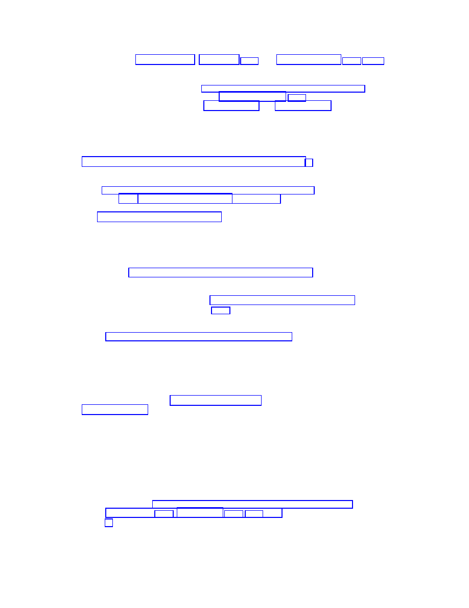
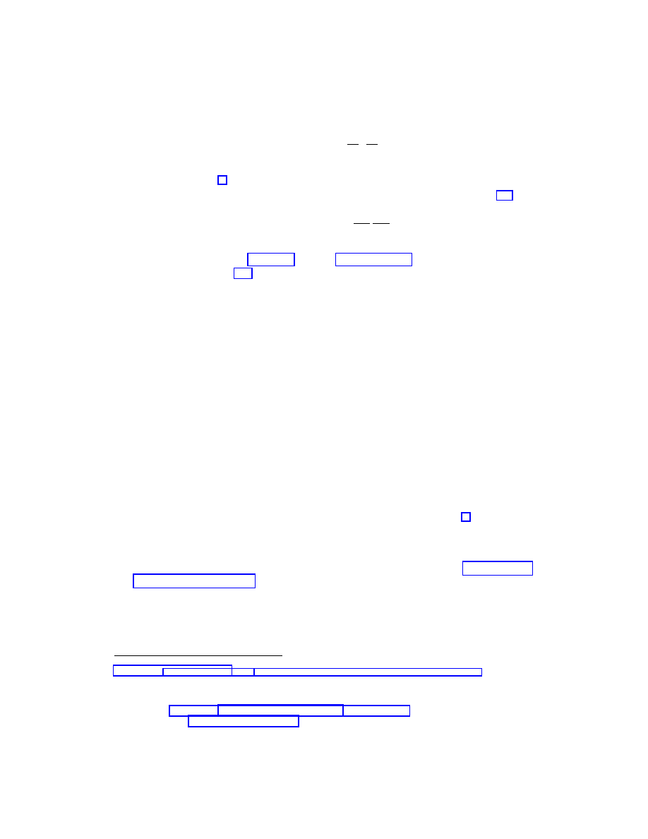
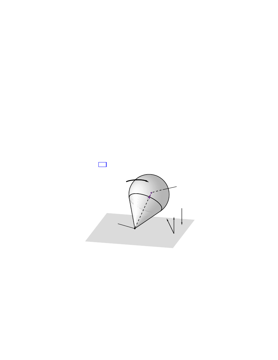
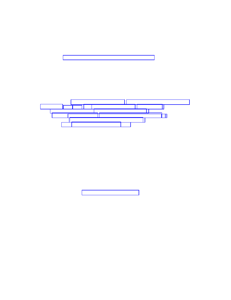
The Heavy Top.
The system is a spinning rigid body with a fixed point in a gravitational
field, as shown in Figure 1.1.
fixed point
Ω
center of mass
l = distance from fixed
point to center of mass
M = total mass
g = gravitational
acceleration
Ω
= body angular
velocity of top
g
lA
χ
k
Γ
Figure 1.1: Heavy top
One usually finds the equations written as:
˙
Π = Π
× Ω + MglΓ × χ
˙
Γ = Γ
× Ω.
Here, M is the body’s mass, Π is the body angular momentum, Ω is the body angular
velocity, g is the acceleration due to gravity, χ is the body fixed unit vector on the line
segment connecting the fixed point with the body’s center of mass, and l is the length of
1.7 Examples
15
this segment. Also, I is the (time independent) moment of inertia tensor in body coordinates,
defined as in the case of the free rigid body. The body angular momentum and the body
angular velocity are related, as before, by Π = IΩ. Also, Γ = A
−1
k, which may be thought
of as the (negative) direction of gravity as seen from the body, where k points upward and
A is the element of SO(3) describing the current configuration of the body.
For a discussion of the Lie–Poisson nature of these equations on the dual of the Lie
algebra se(3) of the Euclidean group and for further references, see Marsden and Ratiu
[1999]. For the Euler–Poincar´
e point of view, see Holm, Marsden and Ratiu [1998a]. These
references also discuss this example from the semidirect product point of view, the theory
of which we shall present shortly.
Now we discuss the shape space, the momentum map, the locked inertia tensor, and the
mechanical connection for this example. We choose Q = SO(3) and G = S
1
, regarded as
rotations about the spatial z-axis, that is, rotations about the axis of gravity.
The shape space is Q/G = S
2
, the two sphere. Notice that in this case, the bundle
π
Q,G
: SO(3)
→ S
2
given by A
∈ SO(3) → Γ = A
−1
k is not a trivial bundle. That is, the
angle of rotation φ about the z-axis is not a global cyclic variable. In other words, in this
case, Q cannot be written as the product S
2
× S
1
. The classical Routh procedure usually
assumes, often implicitly, that the cyclic variables are global.
As with the free rigid body, the heavy top kinetic energy is given by the left invariant
metric on Q = SO(3) whose value at the identity is
Ω
1
, Ω
2
= IΩ
1
·Ω
2
, where Ω
1
, Ω
2
∈ R
3
are thought of as elements of so(3). This kinetic energy is thus left invariant under the action
of the full group SO(3).
The potential energy is given by M glA
−1
k
· χ. This potential energy is invariant under
the group G = S
1
. As usual, the Lagrangian is the kinetic minus the potential energies.
We next compute the infinitesimal generators for the action of G. We identify the Lie
algebra of G with the real line
R and this is identified with the (trivial) subalgebra of so(3)
by ξ
→ ξˆk. These are given, according to the definitions, by ξ
SO(3)
(A) = ξ ˆ
kA
∈ T
A
SO(3).
The locked inertia tensor is, for each A
∈ SO(3), a linear map I(A) : R → R which we
identify with a real number. According to the definitions, it is given by
I(A)ξη =
I(A)ξ, η = ξ
Q
(A), η
Q
(A)
=
ξ ˆ
kA, ηˆ
kA
.
Using the definition of the metric and its left SO(3)-invariance, this equals
ξ ˆ
kA, ηˆ
kA
= ξη
A
−1
ˆ
kA, A
−1
ˆ
kA
= ξη
A
−1
k, A
−1
k
= ξη
AIA
−1
k
· k.
Thus, I(A) =
AIA
−1
k
· k, that is, the (3, 3)-component of the matrix AIA
−1
.
Next, we compute the momentum map J
L
: T SO(3)
→ R for the action of G. According
to the general definition, namely,
J
L
(v
q
), ξ
= v
q
, ξ
Q
(q)
, we get
J
L
(A, ˙
A), ξ
=
˙A, ξˆkA
A
= ξ
A
−1
˙
A, A
−1
ˆ
kA
= ξ
Ω, A
−1
k
.
Using the definition of the metric, we get
ξ
Ω, A
−1
k
= ξ(IΩ)
· (A
−1
k) = ξ(AΠ)
· k = ξπ
3
,
where π = AΠ is the spatial angular momentum. Thus, J
L
(A, ˙
A) = π
3
, the third compo-
nent of the spatial angular momentum. The mechanical connection A(A) : T
A
SO(3)
→ R
is given, using the general formula A(v
q
) = I(q)
−1
J
L
(v
q
), by A(A, ˙
A) = π
3
/
AIA
−1
k
· k.
1.7 Examples
16
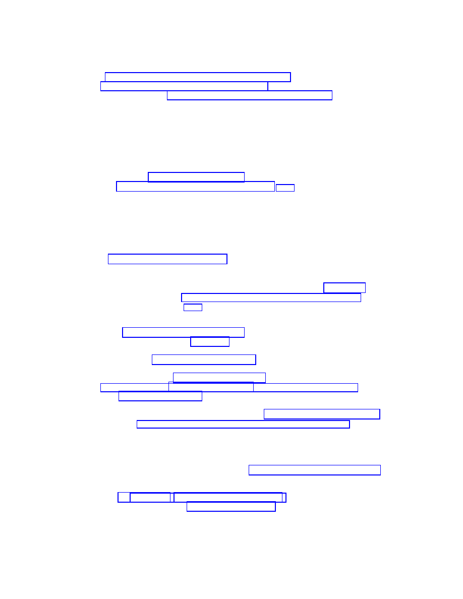
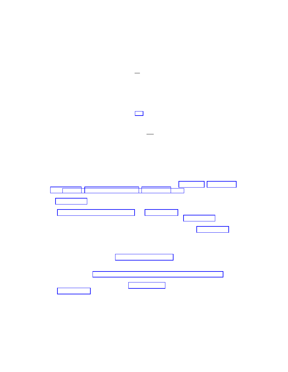
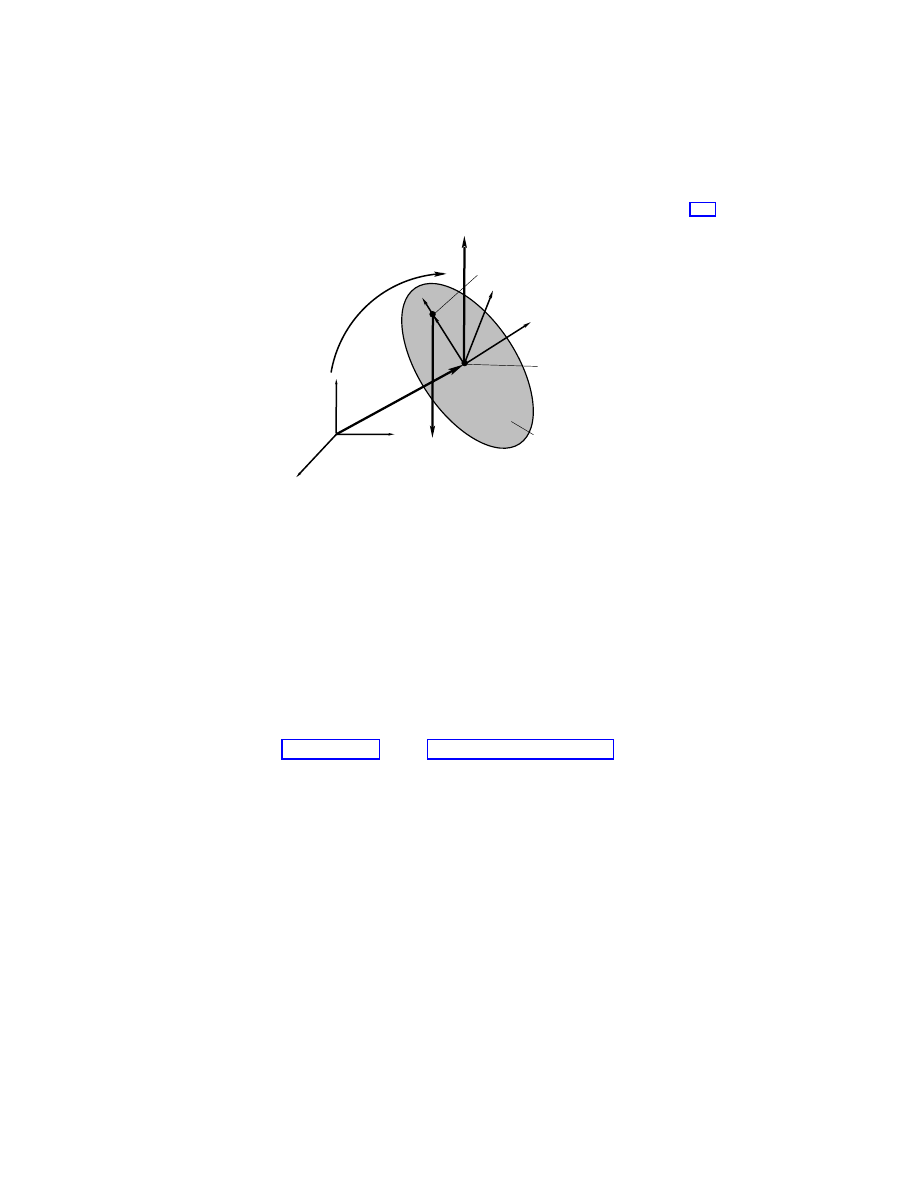
Underwater Vehicle.
The underwater vehicle is modeled as a rigid body moving in ideal
potential flow according to Kirchhoff’s equations. The vehicle is assumed to be neutrally
buoyant (often ellipsoidal), but not necessarily with coincident centers of gravity and buoy-
ancy. The vehicle is free to both rotate and translate in space.
Fix an orthonormal coordinate frame to the body with origin located at the center of
buoyancy and axes aligned with the principal axes of the displaced fluid (Figure 1.2).
inertial frame
body fixed frame
mg (buoyant force)
center of gravity
center of buoyancy
lA
χ
mg
vehicle
b
k
A
Figure 1.2:
Schematic ofa neutrally buoyant ellipsoidal underwater vehicle.
When these axes are also the principal axes of the body and the vehicle is ellipsoidal,
the inertia and mass matrices are simultaneously diagonalized. Let the inertia matrix of
the body-fluid system be denoted by I = diag(I
1
, I
2
, I
3
) and the mass matrix by M =
diag(m
1
, m
2
, m
3
); these matrices include the “added” inertias and masses due to the fluid.
The total mass of the body is denoted m and the acceleration of gravity is g.
The current position of the body is given by a vector b (the vector from the spatially
fixed origin to the center of buoyancy) and its attitude is given by a rotation matrix A (the
center of rotation is the spatial origin). The body fixed vector from the center of buoyancy
to the center of gravity is denoted lχ, where l is the distance between these centers.
We shall now formulate the structure of the problem in a form relevant for the present
needs, omitting the discussion of how one obtains the equations and the Lagrangian. We
refer the reader to Leonard [1997] and to Leonard and Marsden [1997] for additional details.
In particular, these references study the formulation of the equations as Euler–Poincar´
e and
Lie–Poisson equations on a double semidirect product and do a stability analysis.
In this problem, Q = SE(3), the group of Euclidean motions in space, the symmetry
group is G = SE(2)
× R, and G acts on Q on the left as a subgroup; the symmetries corre-
spond to translation and rotation in a horizontal plane together with vertical translations.
Because the centers of gravity and buoyancy are different, rotations around non vertical
axes are not symmetries, as with the heavy top.
The shape space is Q/G = S
2
, as in the case of the heavy top because the quotient
operation removes the translational variables. The bundle π
Q,G
: SO(3)
→ S
2
is again given
by A
∈ SO(3) → Γ = A
−1
k, where Γ has the same interpretation as it did in the case of
the heavy top.
Elements of SE(3) are pairs (A, b) where A
∈ SO(3) and b ∈ R
3
. If the pair (A, b) is
identified with the matrix
A
b
0
1
, then, as is well-known, group multiplication in SE(3)
is given by matrix multiplication. The Lie algebra of SE(3) is se(3) =
R
3
× R
3
with the
1.7 Examples
17
bracket [(Ω, u), (Σ, v)] = (Ω
× Σ, Ω × v − Σ × u).
As shown in the cited references, the underwater vehicle kinetic energy is that of the left
invariant metric on SE(3) given at the identity as follows.
(Ω
1
, v
1
), (Ω
2
, v
2
)
= Ω
1
· IΩ
2
+ Ω
1
· Dv
2
+ v
1
· D
T
Ω
2
+ v
1
· Mv
2
,
(1.12)
where D = m ˆ
χ. The kinetic energy is thus the SE(3) invariant function on T SE(3) whose
value at the identity is given by
K(Ω, v) =
1
2
Ω
· IΩ + Ω · Dv +
1
2
v
· Mv.
The potential energy is given by V (A, b) = mglA
−1
k
· χ and L = K − V .
The momenta conjugate to Ω and v are given by
Π =
∂L
∂Ω
= IΩ + Dv
and
P =
∂L
∂v
= M v + D
T
Ω,
the “angular momentum” and the “linear momentum”. Equivalently, Ω = AΠ + B
T
P and
v = CP + BΠ, where
A = (I
− DM
−1
D
T
)
−1
, B =
−CD
T
I
−1
=
−M
−1
D
T
A, C = (M
− D
T
I
−1
D)
−1
.
The equations of motion are computed to be
˙
Π = Π
× Ω + P × v − mglΓ × χ,
˙
P = P
× Ω,
˙
Γ = Γ
× Ω.
(1.13)
which is the Lie–Poisson (or Euler–Poincar´
e) form in a double semidirect product.
The Lie algebra of G is se(2)
× R, identified with the set of pairs (ξ, v) where ξ ∈ R and
v
∈ R
3
and this is identified with the subalgebra of se(3) of elements of the form (ξ ˆ
k, v).
The infinitesimal generators for the action of G are given by
(ξ, v)
SE(3)
(A, b) = (ξ ˆ
kA, ξk
× b + v) ∈ T
(A,b)
SE(3).
The locked inertia tensor is, for each (A, b)
∈ SE(3), a linear map I(A, b) : so(2) × R →
(so(2)
× R)
∗
. We identify, as above, the Lie algebra g with pairs (ξ, v) and identify the dual
space with the algebra itself using ordinary multiplication and the Euclidean dot product.
According to the definitions, I is given by
I(A, b)(ξ, v), (η, w) =
(ξ, v)
SE(3)
(A, b), (η, w)
SE(3)
(A, b)
(A,b)
=
(ξ ˆ
kA, ξk
× b + v), (ηˆkA, ηk × b + w)
(A,b)
.
The tangent of left translation on the group SE(3) is given by T L
(A,b)
(U, w) = (AU, Aw).
Using the fact that the metric is left SE(3) invariant and formula (1.12) for the inner product,
we arrive at
I(A, b)
· (ξ, v) =
ξ(AIA
−1
k)
· k + ξ(ADA
−1
k)
· k
+
ADA
−1
(ξk
× b + v)
· k +
AM A
−1
(ξk
× b + v)
· (k × b),
AD
T
A
−1
k + AM A
−1
(ξk
× b + v)
.
(1.14)
The momentum map J
L
: T SE(3)
→ se(2)
∗
× R for the action of G is readily computed
using the general definition, namely,
J
L
(v
q
), ξ
= v
q
, ξ
Q
(q)
; one gets
J
L
(A, b, ˙
A, ˙b) = ((AΠ + b
× AP) · k, AP),
2 The Bundle Picture in Mechanics
18
where, recall, Π = ∂L/∂Ω = IΩ + Dv and P = ∂L/∂v = M v + D
T
Ω.
The mechanical connection A(A, b) : T
(A,b)
SE(3)
→ se(2)
∗
× R is therefore given,
according to the general formula A(v
q
) = I(q)
−1
J
L
(v
q
), by
A(A, b, ˙
A, ˙b) = I(A, b)
−1
· ((AΠ + b × AP) · k, AP)
where I(A, b) is given by (1.14). We do not attempt to invert the locked inertia tensor
explicitly in this case.
2
The Bundle Picture in Mechanics
2.1
Cotangent Bundle Reduction
Cotangent bundle reduction theory lies at the heart of the bundle picture. We will describe
it from this point of view in this section.
Some History.
We continue the history given in the introduction concerning cotangent
bundle reduction. From the symplectic viewpoint, a principal result is that the symplectic
reduction of a cotangent bundle T
∗
Q at µ
∈ g
∗
is a bundle over T
∗
(Q/G) with fiber the
coadjoint orbit through µ. This result can be traced back, in a preliminary form, to Sternberg
[1977], and Weinstein [1977]. This was developed in the work of Montgomery, Marsden and
Ratiu [1984] and Montgomery [1986]; see the discussions in Abraham and Marsden [1978],
Marsden [1981] and Marsden [1992]. It was shown in Abraham and Marsden [1978] that the
symplectically reduced cotangent bundle can be symplectically embedded in T
∗
(Q/G
µ
)—
this is the injective version of the cotangent bundle reduction theorem. From the Poisson
viewpoint, in which one simply takes quotients by group actions, this reads: (T
∗
Q)/G is a
g
∗
-bundle over T
∗
(Q/G), or a Lie–Poisson bundle over the cotangent bundle of shape space.
We shall return to this bundle point of view shortly and sharpen some of these statements.
The Bundle Point of View.
We choose a principal connection
A on the shape space
bundle.
Define ˜
g = (Q
× g)/G, the associated bundle to g, where the quotient uses
the given action on Q and the coadjoint action on g. The connection
A defines a bundle
isomorphism α
A
: T Q/G
→ T (Q/G) ⊕ ˜g given by α
A
([v
q
]
G
) = T π
Q,G
(v
q
)
⊕ [q, A(v
q
)]
G
.
Here, the sum is a Whitney sum of vector bundles over Q/G (the fiberwise direct sum)
and the symbol [q,
A(v
q
)]
G
means the equivalence class of (q,
A(v
q
))
∈ Q × g under the
G-action. The map α
A
is a well-defined vector bundle isomorphism with inverse given by
α
−1
A
(u
x
⊕ [q, ξ]
G
) = [(u
x
)
h
q
+ ξ
Q
(q)]
G
, where (u
x
)
h
q
denotes the horizontal lift of u
x
to the
point q.
Poisson Cotangent Bundle Reduction.
The bundle view of Poisson cotangent bundle
reduction considers the inverse of the fiberwise dual of α
A
, which defines a bundle isomor-
phism (α
−1
A
)
∗
: T
∗
Q/G
→ T
∗
(Q/G)
⊕ ˜g
∗
, where ˜
g
∗
= (Q
× g
∗
)/G is the vector bundle over
Q/G associated to the coadjoint action of G on g
∗
. This isomorphism makes explicit the
sense in which (T
∗
Q)/G is a bundle over T
∗
(Q/G) with fiber g
∗
. The Poisson structure
on this bundle is a synthesis of the canonical bracket, the Lie–Poisson bracket, and curva-
ture. The inherited Poisson structure on this space was derived in Montgomery, Marsden
and Ratiu [1984] (details were given in Montgomery [1986]) and was put into the present
context in Cendra, Marsden and Ratiu [2000a].
5
The general theory, in principle, does not require one to choose a connection. However, there are many
good reasons to do so, such as applications to stability theory and geometric phases.
2.2 Lagrange-Poincar´
e Reduction
19
Symplectic Cotangent Bundle Reduction.
?] show that each symplectic reduced
space of T
∗
Q, which are the symplectic leaves in (T
∗
Q)/G ∼
= T
∗
(Q/G)
⊕ ˜g
∗
, are given by
a fiber product T
∗
(Q/G)
×
Q/G
O, where
O is the associated coadjoint orbit bundle. This
makes precise the sense in which the symplectic reduced spaces are bundles over T
∗
(Q/G)
with fiber a coadjoint orbit. They also give an intrinsic expression for the reduced symplectic
form, which involves the canonical symplectic structure on T
∗
(Q/G), the curvature of the
connection, the coadjoint orbit symplectic form, and interaction terms that pair tangent
vectors to the orbit with the vertical projections of tangent vectors to the configuration
space; see also Zaalani [1999].
As we shall show in the next section, the reduced space P
µ
for P = T
∗
Q is globally
diffeomorphic to the bundle T
∗
(Q/G)
×
Q/G
Q/G
µ
, where Q/G
µ
is regarded as a bundle
over Q/G. In fact, these results simplify the study of these symplectic leaves. In particular,
this makes the injective version of cotangent bundle reduction transparent. Indeed, there
is a natural inclusion map T
∗
(Q/G)
×
Q/G
Q/G
µ
→ T
∗
(Q/G
µ
), induced by the dual of the
tangent of the projection map ρ
µ
: Q/G
µ
→ Q/G. This inclusion map then realizes the
reduced spaces P
µ
as symplectic subbundles of T
∗
(Q/G
µ
).
2.2
Lagrange-Poincar´
e Reduction
In a local trivialization, write Q = S
× G where S = Q/G, and T Q/G as T S × g. Coor-
dinates on Q are written x
α
, s
a
and those for (T Q)/G are denoted (x
α
, ˙x
α
, ξ
a
). Locally,
the connection one form on Q is written ds
a
+
A
a
α
dx
α
and we let Ω
a
= ξ
a
+
A
a
α
˙x
α
. The
components of the curvature of
A are
B
b
αβ
=
∂A
b
β
∂x
α
−
∂A
b
α
∂x
β
− C
b
cd
A
c
α
A
d
β
,
where C
a
bd
are the structure constants of the Lie algebra g. Later, in the text, we review the
intrinsic definition of curvature.
Let, as explained earlier, L : T Q
→ R be a G-invariant Lagrangian and let l : (T Q)/G →
R be the corresponding function induced on (T Q)/G. The Euler–Lagrange equations on Q
induce equations on this quotient space. The connection is used to write these equations in-
trinsically as a coupled set of Euler–Lagrange type equations and Euler–Poincar´
e equations.
These reduced Euler–Lagrange equations, also called the Lagrange-Poincar´
e equa-
tions (implicitly contained in Cendra, Ibort and Marsden [1987] and explicitly in Marsden
and Scheurle [1993b]) are, in coordinates,
d
dt
∂l
∂ ˙x
α
−
∂l
∂x
α
=
∂l
∂Ω
a
B
a
αβ
˙x
β
− C
a
db
A
b
α
Ω
d
d
dt
∂l
∂Ω
b
=
∂l
∂Ω
a
C
a
db
Ω
d
− C
a
db
A
d
α
˙x
α
Using the geometry of the bundle T Q/G ∼
= T (Q/G)
⊕ ˜g, one can write these equations
intrinsically in terms of covariant derivatives (see Cendra, Marsden and Ratiu [2000a]).
Namely, they take the form
∂l
∂x
(x, ˙x, ¯
v)
−
D
Dt
∂l
∂ ˙x
(x, ˙x, ¯
v) =
∂l
∂¯
v
(x, ˙x, ¯
v), i
˙
x
Curv
A
(x)
D
Dt
∂l
∂¯
v
(x, ˙x, ¯
v) = ad
∗
¯
v
∂l
∂¯
v
(x, ˙x, ¯
v) .
The first of these equations is the horizontal Lagrange–Poincar´
e equation while the
second is the vertical Lagrange–Poincar´
e equation. The notation here is as follows.
2.3 Hamiltonian Semidirect Product Theory
20
Points in T (Q/G)
⊕ ˜g are denoted (x, ˙x, ¯v) and l(x, ˙x, ¯v) denotes the Lagrangian induced
on the quotient space from L. The bundles T (Q/G)
⊕ ˜g naturally inherit vector bundle
connections and D/Dt denotes the associated covariant derivatives. Also, Curv
A
denotes
the curvature of the connection
A thought of as an adjoint bundle valued two form on
Q/G—basic definitions and properties of curvature will be reviewed shortly.
Lagrangian Reduction by Stages.
The perspective developed in Cendra, Marsden and
Ratiu [2000a] is motivated by reduction by stages. In fact, that work develops a context (of
Lagrange–Poincar´e bundles) in which Lagrangian reduction can be repeated. In particular,
this theory treats successive reduction for group extensions. Reduction for group extensions,
in turn, builds on semidirect product reduction theory, to which we turn next.
2.3
Hamiltonian Semidirect Product Theory
Lie–Poisson Systems on Semidirect Products.
The study of Lie–Poisson equations
for systems on the dual of a semidirect product Lie algebra grew out of the work of many
authors including Sudarshan and Mukunda [1974], Vinogradov and Kuperschmidt [1977],
Ratiu [1980a, 1981, 1982], Guillemin and Sternberg [1980], Marsden [1982], Marsden, Wein-
stein, Ratiu and Schmid [1983], Holm and Kuperschmidt [1983], Kuperschmidt and Ratiu
[1983], Holmes and Marsden [1983], Marsden, Ratiu and Weinstein [1984a,b], Guillemin and
Sternberg [1984], Holm, Marsden, Ratiu and Weinstein [1985], Abarbanel, Holm, Marsden
and Ratiu [1986], Leonard and Marsden [1997], and Marsden, Misiolek, Perlmutter and
Ratiu [1998]. As these and related references show, the Lie–Poisson equations apply to
a surprisingly wide variety of systems such as the heavy top, compressible flow, stratified
incompressible flow, MHD (magnetohydrodynamics), and underwater vehicle dynamics.
In each of the above examples as well as in the general theory, one can view the given
Hamiltonian in the material representation as a function depending on a parameter; this
parameter becomes a dynamic variable when reduction is performed. For example, in the
heavy top, the direction and magnitude of gravity, the mass and location of the center of
mass may be regarded as parameters, but the direction of gravity becomes the dynamic
variable Γ when reduction is performed.
We first recall how the Hamiltonian theory proceeds for systems defined on semidirect
products. We present the abstract theory, but of course historically this grew out of the
examples, especially the heavy top and compressible flow. When working with various
models of continuum mechanics and plasmas one has to keep in mind that many of the
actions are right actions, so one has to be careful when employing general theorems involving
left actions. We refer to Holm, Marsden and Ratiu [1998a] for a statement of some of the
results explicitly for right actions.
Generalities on Semidirect Products.
Let V be a vector space and assume that the
Lie group G acts on the left by linear maps on V (and hence G also acts on on the left on
its dual space V
∗
). The semidirect product S = G
V is the set S = G × V with group
multiplication given by (g
1
, v
1
)(g
2
, v
2
) = (g
1
g
2
, v
1
+ g
1
v
2
), where the action of g
∈ G on
v
∈ V is denoted gv. The identity element is (e, 0) where e is the identity in G and the
inverse of (g, v) is (g, v)
−1
= (g
−1
,
−g
−1
v). The Lie algebra of S is the semidirect product
Lie algebra, s = g
V , whose bracket is [(ξ
1
, v
1
), (ξ
2
, v
2
)] = ([ξ
1
, ξ
2
], ξ
1
v
2
− ξ
2
v
1
) , where we
denote the induced action of g on V by ξ
1
v
2
.
The adjoint and coadjoint actions are given by
(g, v)(ξ, u) = (gξ, gu
− (gξ)v) and (g, v)(µ, a) = (gµ + ρ
∗
v
(ga), ga),

2.3 Hamiltonian Semidirect Product Theory
21
where (g, v)
∈ S = G×V , (ξ, u) ∈ s = g×V , (µ, a) ∈ s
∗
= g
∗
×V
∗
, gξ = Ad
g
ξ, gµ = Ad
∗
g
−1
µ,
ga denotes the induced left action of g on a (the left action of G on V induces a left action
of G on V
∗
— the inverse of the transpose of the action on V ), ρ
v
: g
→ V is the linear map
given by ρ
v
(ξ) = ξv, and ρ
∗
v
: V
∗
→ g
∗
is its dual. For a
∈ V
∗
, we write ρ
∗
v
a = v
a ∈ g
∗
,
which is a bilinear operation in v and a. Equivalently, we can write
ηa, v = − v a , η .
Using this notation, the coadjoint action reads (g, v)(µ, a) = (gµ + v
(ga), ga).
Lie–Poisson Brackets and Hamiltonian Vector Fields.
For a left representation of
G on V the
± Lie–Poisson bracket of two functions f, k : s
∗
→ R is given by
{f, k}
±
(µ, a) =
±
µ,
δf
δµ
,
δk
δµ
±
a,
δf
δµ
δk
δa
−
δk
δµ
δf
δa
where δf /δµ
∈ g, and δf/δa ∈ V are the functional derivatives of f. The Hamiltonian
vector field of h : s
∗
→ R has the expression
X
h
(µ, a) =
∓
ad
∗
δh/δµ
µ
−
δh
δa
a, −
δh
δµ
a
.
Thus, Hamilton’s equations on the dual of a semidirect product are given by
˙µ =
∓ ad
∗
δh/δµ
µ
±
δh
δa
a ,
˙a =
±
δh
δµ
a .
Symplectic Actions by Semidirect Products.
Consider a left symplectic action of S
on a symplectic manifold P that has an equivariant momentum map J
S
: P
→ s
∗
. Since
V is a (normal) subgroup of S, it also acts on P and has a momentum map J
V
: P
→ V
∗
given by J
V
= i
∗
V
◦ J
S
, where i
V
: V
→ s is the inclusion v → (0, v) and i
∗
V
: s
∗
→ V
∗
is
its dual. We think of J
V
as the second component of J
S
. We can regard G as a subgroup
of S by g
→ (g, 0). Thus, G also has a momentum map that is the first component of J
S
but this will play a secondary role in what follows. Equivariance of J
S
under G implies that
J
V
(gz) = gJ
V
(z). To prove this relation, one uses the fact that for the coadjoint action of
S on s
∗
the second component is the dual of the given action of G on V .
The Classical Semidirect Product Reduction Theorem.
In a number of interesting
applications such as compressible fluids, the heavy top, MHD, etc., one has two symmetry
groups that do not commute and thus the commuting reduction by stages theorem of Marsden
and Weinstein [1974] does not apply. In this more general situation, it matters in what order
one performs the reduction, which occurs, in particular for semidirect products. The main
result covering the case of semidirect products has a complicated history, with important
early contributions by many authors, as we have listed above. The final version of the
theorem as we shall use it, is due to Marsden, Ratiu and Weinstein [1984a,b].
Theorem 2.1 (Semidirect Product Reduction Theorem).
Let S = G
V , choose
σ = (µ, a)
∈ g
∗
× V
∗
, and reduce T
∗
S by the action of S at σ giving the coadjoint orbit
O
σ
through σ
∈ s
∗
. There is a symplectic diffeomorphism between
O
σ
and the reduced space
obtained by reducing T
∗
G by the subgroup G
a
(the isotropy of G for its action on V
∗
at the
point a
∈ V
∗
) at the point µ
|g
a
where g
a
is the Lie algebra of G
a
.
This theorem is a consequence of a more general result given in the next section.

2.4 Semidirect Product Reduction by Stages
22
2.4
Semidirect Product Reduction by Stages
A theorem on reduction by stages for semidirect products acting on a symplectic manifold is
due to Leonard and Marsden [1997] (where the motivation was the application to underwater
vehicle dynamics) and Marsden, Misiolek, Perlmutter and Ratiu [2000].
Consider a symplectic action of S on a symplectic manifold P that has an equivariant
momentum map J
S
: P
→ s
∗
. As we have explained, the momentum map for the action of
V is the map J
V
: P
→ V
∗
given by J
V
= i
∗
V
◦ J
S
We carry out the reduction of P by S at a regular value σ = (µ, a) of the momentum
map J
S
for S in two stages. First, reduce P by V at the value a (assume it to be a regular
value) to get the reduced space P
a
= J
−1
V
(a)/V . Second, form the isotropy group G
a
of
a
∈ V
∗
. One shows (this step is not trivial) that the group G
a
acts on P
a
and has an
induced equivariant momentum map J
a
: P
a
→ g
∗
a
, where g
a
is the Lie algebra of G
a
, so one
can reduce P
a
at the point µ
a
:= µ
|g
a
to get the reduced space (P
a
)
µ
a
= J
−1
a
(µ
a
)/(G
a
)
µ
a
.
Theorem 2.2 (Reduction by Stages for Semidirect Products.). The reduced space
(P
a
)
µ
a
is symplectically diffeomorphic to the reduced space P
σ
obtained by reducing P by S
at the point σ = (µ, a).
Combined with the cotangent bundle reduction theorem, the semidirect product reduc-
tion theorem is a useful tool. For example, this shows that the generic coadjoint orbits for
the Euclidean group are cotangent bundles of spheres with the associated coadjoint orbit
symplectic structure given by the canonical structure plus a magnetic term.
Semidirect Product Reduction of Dynamics.
There is a technique for reducing dy-
namics that is associated with the geometry of the semidirect product reduction theorem.
One proceeds as follows.
We start with a Hamiltonian H
a
0
on T
∗
G that depends parametrically on a variable
a
0
∈ V
∗
. The Hamiltonian, regarded as a map H : T
∗
G
× V
∗
→ R is assumed to be
invariant on T
∗
G
× V
∗
under the action of G on T
∗
G
× V
∗
. One shows that this condition
is equivalent to the invariance of the function H defined on T
∗
S = T
∗
G
× V × V
∗
ex-
tended to be constant in the variable V under the action of the semidirect product. By the
semidirect product reduction theorem, the dynamics of H
a
0
reduced by G
a
0
, the isotropy
group of a
0
, is symplectically equivalent to Lie–Poisson dynamics on s
∗
= g
∗
× V
∗
. The
Lie–Poisson structure determines the reduced dynamics (given explicitly above) using the
function h(µ, a) = H(α
g
, g
−1
a) where µ = g
−1
α
g
.
2.5
Lagrangian Semidirect Product Theory
Lagrangian semidirect product reduction is modeled after the reduction theorem for the basic
Euler–Poincar´
e equations, although they are not literally special cases of it. To distinguish
these, we use phrases like basic Euler–Poincar´
e equations for the equations (1.6) and simply
the Euler–Poincar´
e equations or the Euler–Poincar´
e equations with advection or the Euler–
Poincar´e equations with advected parameters, for the equations that follow.
The main difference between the invariant Lagrangians considered in the Euler–Poincar´
e
reduction theorem earlier and the ones we work with now is that L and l depend on an
additional parameter a
∈ V
∗
, where V is a representation space for the Lie group G and L
has an invariance property relative to both arguments.
The parameter a
∈ V
∗
acquires dynamical meaning under Lagrangian reduction as it
did for the Hamiltonian case: ˙a =
± (δh/δµ)a. For the heavy top, the parameter is the
unit vector Γ in the (negative) direction of gravity, which becomes a dynamical variable in
body representation. For compressible fluids, a becomes the density of the fluid in spatial
representation, which becomes a dynamical variable (satisfying the continuity equation).
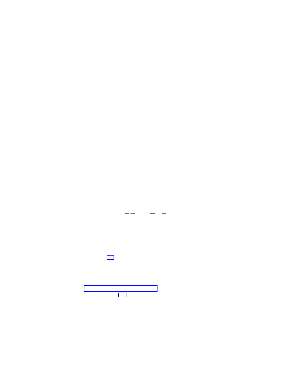
2.5 Lagrangian Semidirect Product Theory
23
The basic ingredients are as follows. There is a left representation of the Lie group G
on the vector space V and G acts in the natural way on the left on T G
× V
∗
: h(v
g
, a) =
(hv
g
, ha). Assume that the function L : T G
× V
∗
→ R is left G–invariant. In particular,
if a
0
∈ V
∗
, define the Lagrangian L
a
0
: T G
→ R by L
a
0
(v
g
) = L(v
g
, a
0
). Then L
a
0
is left invariant under the lift to T G of the left action of G
a
0
on G, where G
a
0
is the
isotropy group of a
0
. Left G–invariance of L permits us to define l : g
× V
∗
→ R by
l(g
−1
v
g
, g
−1
a
0
) = L(v
g
, a
0
). Conversely, this relation defines for any l : g
× V
∗
→ R a left
G–invariant function L : T G
× V
∗
→ R. For a curve g(t) ∈ G, let ξ(t) := g(t)
−1
˙g(t) and
define the curve a(t) as the unique solution of the following linear differential equation with
time dependent coefficients ˙a(t) =
−ξ(t)a(t), with initial condition a(0) = a
0
. The solution
can be written as a(t) = g(t)
−1
a
0
.
Theorem 2.3. With the preceding notation, the following are equivalent:
(i) With a
0
held fixed, Hamilton’s variational principle
δ
t
2
t
1
L
a
0
(g(t), ˙g(t))dt = 0
(2.1)
holds, for variations δg(t) of g(t) vanishing at the endpoints;
(ii) g(t) satisfies the Euler–Lagrange equations for L
a
0
on G;
(iii) The constrained variational principle;
δ
t
2
t
1
l(ξ(t), a(t))dt = 0
(2.2)
holds on g
× V
∗
, using variations of ξ and a of the form δξ = ˙η + [ξ, η] and δa =
−ηa,
where η(t)
∈ g vanishes at the endpoints;
(iv) The Euler–Poincar´
e equations hold on g
× V
∗
d
dt
δl
δξ
= ad
∗
ξ
δl
δξ
+
δl
δa
a.
(2.3)
Remarks:
1. As with the basic Euler–Poincar´
e equations, this is not strictly a variational principle
in the same sense as the standard Hamilton’s principle. It is more of a Lagrange–d’Al-
embert principle, because we impose the stated constraints on the variations allowed;
2. Note that equations (2.3) are not the basic Euler–Poincar´
e equations because we are
not regarding g
× V
∗
as a Lie algebra. Rather, these equations are thought of as
a generalization of the classical Euler–Poisson equations for a heavy top, written in
body angular velocity variables, as we shall see in the examples. Some authors may
prefer the term Euler–Poisson–Poincar´
e equations for these equations.
We refer to Holm, Marsden and Ratiu [1998a] for the proof. It is noteworthy that
these Euler–Poincar´e equations (2.3) are not the (pure) Euler–Poincar´
e equations for the
semidirect product Lie algebra g
V
∗
2.5 Lagrangian Semidirect Product Theory
24
The Legendre Transformation.
Start with a Lagrangian on g
× V
∗
and perform a
partial Legendre transformation in the variable ξ only, by writing
µ =
δl
δξ
,
h(µ, a) =
µ, ξ − l(ξ, a).
Since
δh
δµ
= ξ +
µ,
δξ
δµ
−
δl
δξ
,
δξ
δµ
= ξ ,
and δh/δa =
−δl/δa, we see that (2.3) and ˙a(t) = −ξ(t)a(t) imply the Lie–Poisson dynamics
on a semidirect product for the minus Lie–Poisson bracket. If this Legendre transformation
is invertible, then we can also pass from the the minus Lie–Poisson equations to the Euler–
Poincar´e equations (2.3) together with the equations ˙a(t) =
−ξ(t)a(t).
Relation with Lagrangian Reduction.
The Euler–Poincar´e equations are shown to
be a special case of the reduced Euler–Lagrange equations in Cendra, Holm, Marsden and
Ratiu [1998]. We also refer to Cendra, Holm, Marsden and Ratiu [1998] who study the
Euler–Poincar´
e formulation of the Maxwell–Vlasov equations for plasma physics.
The Kelvin–Noether Theorem.
There is a version of the Noether theorem that holds
for solutions of the Euler–Poincar´
e equations. Our formulation is motivated by and designed
for ideal continuum theories (and hence the name Kelvin–Noether), but it may be also of
interest for finite dimensional mechanical systems. Of course it is well known (going back at
least to Arnold [1966a]) that the Kelvin circulation theorem for ideal flow is closely related
to the Noether theorem applied to continua using the particle relabeling symmetry group.
Start with a Lagrangian L
a
0
depending on a parameter a
0
∈ V
∗
as above and introduce
a manifold
C on which G acts (we assume this is also a left action) and suppose we have
an equivariant map
K : C × V
∗
→ g
∗∗
. In the case of continuum theories, the space
C is
usually a loop space and
K(c, a), µ for c ∈ C and µ ∈ g
∗
will be a circulation. This class
of examples also shows why we do not want to identify the double dual g
∗∗
with g.
Define the Kelvin–Noether quantity I :
C × g × V
∗
→ R by
I(c, ξ, a) =
K(c, a),
δl
δξ
.
(2.4)
Theorem 2.4 (Kelvin–Noether). Fixing c
0
∈ C, let ξ(t), a(t) satisfy the Euler–Poincar´e
equations and define g(t) to be the solution of ˙g(t) = g(t)ξ(t) and, say, g(0) = e. L et
c(t) = g(t)
−1
c
0
and I(t) = I(c(t), ξ(t), a(t)). Then
d
dt
I(t) =
K(c(t), a(t)),
δl
δa
a
.
(2.5)
Again, we refer to Holm, Marsden and Ratiu [1998a] for the proof.
Corollary 2.5. For the basic Euler–Poincar´
e equations, the Kelvin quantity I(t), defined
the same way as above but with I :
C × g → R, is conserved.
The Heavy Top.
As we explained earlier, the heavy top kinetic energy is given by the left
invariant metric on SO(3) whose value at the identity is
Ω
1
, Ω
2
= IΩ
1
·Ω
2
, where Ω
1
, Ω
2
∈
R
3
are thought of as elements of so(3), the Lie algebra of SO(3), via the isomorphism
Ω
∈ R
3
→ ˆ
Ω
∈ so(3), ˆ
Ωv := Ω
× v
2.6 Reduction by Stages
25
This kinetic energy is thus left invariant under SO(3). The potential energy is given by
M glA
−1
k
· χ. This potential energy breaks the full SO(3) symmetry and is invariant only
under the rotations S
1
about the k–axis.
For the application of Theorem 2.3 we think of the Lagrangian of the heavy top as a
function on T SO(3)
× R
3
→ R. Define U(u
A
, v) = M gA A
−1
v
· χ which is verified to
be SO(3)–invariant, so the hypotheses of Theorem 2.3 are satisfied. Thus, the heavy top
equations of motion in the body representation are given by the Euler–Poincar´
e equations
(2.3) for the Lagrangian l : so(3)
× R
3
→ R defined by
l(Ω, Γ) = L(A
−1
u
A
, A
−1
v) =
1
2
Π
· Ω − U(A
−1
u
A
, A
−1
v) =
1
2
Π
· Ω − MgA Γ · χ .
It is then straightforward to compute the Euler–Poincar´
e equations for this reduced La-
grangian and to verify that one gets the usual heavy top equations.
Let
C = g and let K : C × V
∗
→ g
∗∗
∼
= g be the map (W, Γ)
→ W. Then the Kelvin–
Noether theorem gives the statement
d
dt
W, Π = MgA W, Γ × χ ,
where W(t) = A(t)
−1
w; in other words, W(t) is the body representation of a space fixed
vector. This statement is easily verified directly. Also, note that
W, Π = w, π, with
π = A(t)Π, so the Kelvin–Noether theorem may be viewed as a statement about the rate
of change of the momentum map of the system (the spatial angular momentum) relative to
the full group of rotations, not just those about the vertical axis.
2.6
Reduction by Stages
Poisson Reduction by Stages.
Suppose that a Lie group M acts symplectically on a
symplectic manifold P . Let N be a normal subgroup of M (so M is an extension of N ).
The problem is to carry out a reduction of P by M in two steps, first a reduction of P by N
followed by, roughly speaking, a reduction by the quotient group M/N . On a Poisson level,
this is elementary: P/M is Poisson diffeomorphic to (P/N )/(M/N ). However, symplectic
reduction is a much deeper question.
Symplectic Reduction by Stages.
We now state the theorem on symplectic reduction
by stages regarded as a generalization of the semidirect product reduction theorem. We
refer to Marsden, Misiolek, Perlmutter and Ratiu [1998, 2000] and Leonard and Marsden
[1997] for details and applications.
Start with a symplectic manifold (P, Ω) and a Lie group M that acts on P and has an
Ad
∗
-equivariant momentum map J
M
: P
→ m
∗
, where m is the Lie algebra of M . We shall
denote this action by Φ : M
× P → P and the mapping associated with a group element
m
∈ M by Φ
m
: P
→ P .
Assume that N is a normal subgroup of M and denote its Lie algebra by n. Let i : n
→ m
denote the inclusion and let i
∗
: m
∗
→ n
∗
be its dual, which is the natural projection given
by restriction of linear functionals. The equivariant momentum map for the action of the
group N on P is given by J
N
(z) = i
∗
(J
M
(z)). Let ν
∈ n
∗
be a regular value of J
N
and
let N
ν
be the isotropy subgroup of ν for the coadjoint action of N on its Lie algebra. We
suppose that the action of N
ν
(and in fact that of M ) is free and proper and form the first
symplectic reduced space: P
ν
= J
−1
N
(ν)/N
ν
.
Since N is a normal subgroup, the adjoint action of M on its Lie algebra m leaves the
subalgebra n invariant, and so it induces a dual action of M on n
∗
. Thus, we can consider
M
ν
, the isotropy subgroup of ν
∈ n
∗
for the action of M on n
∗
. One checks that the subgroup

3 Routh Reduction
26
N
ν
⊂ M is normal in M
ν
, so we can form the quotient group M
ν
/N
ν
. In the context of
semidirect products, with the second factor being a vector space V , M
ν
/N
ν
reduces to G
a
where ν = a in our semidirect product notation.
Now one shows that there is a well defined symplectic action of M
ν
/N
ν
on the reduced
space P
ν
. In fact, there is a natural sense in which the momentum map J
M
: P
→ m
∗
induces a momentum map J
ν
: P
ν
→ (m
ν
/n
ν
)
∗
for this action. However, this momentum
map in general need not be equivariant.
However, nonequivariant reduction is a well-defined process and so P
ν
can be further
reduced by the action of M
ν
/N
ν
at a regular value ρ
∈ (m
ν
/n
ν
)
∗
. Let this second reduced
space be denoted by P
ν,ρ
= J
−1
M
ν
/N
ν
(ρ)/(M
ν
/N
ν
)
ρ
where, as usual, (M
ν
/N
ν
)
ρ
is the isotropy
subgroup for the action of the group M
ν
/N
ν
on the dual of its Lie algebra.
Assume that σ
∈ m
∗
is a given regular element of J
M
so that we can form the reduced
space P
σ
= J
−1
M
(σ)/M
σ
where M
σ
is the isotropy subgroup of σ for the action of M on m
∗
.
We also require that the relation (r
ν
)
∗
(ρ) = k
∗
ν
σ
− ¯ν holds where r
ν
: m
ν
→ m
ν
/n
ν
is the
quotient map, k
ν
: m
ν
→ m is the inclusion and ¯ν is some extension of ν to m
ν
. We assume
that the following condition holds:
Stages Hypothesis: For all σ
1
, σ
2
∈ m
∗
such that σ
1
|m
ν
= σ
2
|m
ν
and σ
1
|n = σ
2
|n, there
exists n
∈ N
ν
such that σ
2
= Ad
∗
n
−1
σ
1
.
Theorem 2.6 (Symplectic Reduction by Stages.). Under the above hypotheses, there
is a symplectic diffeomorphism between P
σ
and P
ν,ρ
.
Lagrangian Stages.
We will just make some comments on the Lagrangian counterpart
to Hamiltonian reduction by stages. First of all, it should be viewed as a Lagrangian coun-
terpart to Poisson reduction by stages, which, as we have remarked, is relatively straight-
forward. What makes the Lagrangian counterpart more difficult is the a priori lack of a
convenient category, like that of Poisson manifolds, which is stable under reduction. Such
a category, which may be viewed as the minimal category satisfying this property and con-
taining tangent bundles, is given in Cendra, Marsden and Ratiu [2000a]. This category
must, as we have seen, contain bundles of the form T (Q/G)
⊕ g. This gives a clue as to
the structure of the general element of this Lagrange–Poincar´
e category, namely direct
sums of tangent bundles with vector bundles with fiberwise Lie algebra structure and certain
other (curvature-like) structures. In particular, this theory can handle the case of general
group extensions and includes Lagrangian semidirect product reduction as a special case.
The Lagrangian analogue of symplectic reduction is nonabelian Routh reduction to which
we turn next. Developing Routh reduction by stages is an interesting and challenging open
problem.
3
Routh Reduction
Routh reduction differs from Lagrange–Poincar´
e reduction in that the momentum map
constraint J
L
= µ is imposed. Routh dealt with systems having cyclic variables. The heavy
top has an abelian group of symmetries, with a free and proper action, yet it does not have
global cyclic variables in the sense that the bundle Q
→ Q/G is not trivial; that is, Q is not
globally a product S
× G. For a modern exposition of Routh reduction in the case when
Q = S
× G and G is Abelian, see Marsden and Ratiu [1999], §8.9, and Arnold, Kozlov and
Neishtadt [1988].
We shall now embark on a global intrinsic presentation of nonabelian Routh reduction.
Preliminary versions of this theory, which represent our starting point are given in Marsden
and Scheurle [1993a] and Jalnapurkar and Marsden [2000a].

3.1 The Global Realization Theorem for the Reduced Phase Space
27
3.1
The Global Realization Theorem for the Reduced Phase Space
Let G
µ
denote the isotropy subgroup of µ for the coadjoint action of G on g
∗
. Because
G acts freely and properly on Q and assuming that µ is a regular value of the momentum
map J
L
, the space J
−1
L
(µ)/G
µ
is a smooth symplectic manifold (by the symplectic reduction
theorem). The symplectic structure is not of immediate concern to us.
Fiber Products.
Given two fiber bundles f : M
→ B and g : N → B, the fiber product
is M
×
B
N =
{(m, n) ∈ M ×N | f(m) = g(n)}. Using the fact that M ×
B
N = (f
×g)
−1
(∆)
where ∆ is the diagonal in B
× B, one sees that M ×
B
N is a smooth submanifold of M
× N
and a smooth fiber bundle over B with the projection map (m, n)
→ f(m) = g(n).
Statement of the Global Realization Theorem.
Consider the two fiber bundles τ
Q/G
:
T (Q/G)
→ Q/G and ρ
µ
: Q/G
µ
→ Q/G. The first is the tangent bundle of shape space,
while the second is the map taking an equivalence class with respect to the G
µ
group action
and mapping it to the larger class (orbit) for the G action on Q. We write the map ρ
µ
as
[q]
G
µ
→ [q]
G
. The map ρ
µ
is smooth being the quotient map induced by the identity. We
form the fiber product bundle p
µ
: T (Q/G)
×
Q/G
Q/G
µ
→ Q/G.
A couple of remarks about the bundle structures are in order. The fibers of the bundle
ρ
µ
: Q/G
µ
→ Q/G are diffeomorphic to the coadjoint orbit O
µ
through µ for the G action
on g
∗
, that is, to the homogeneous quotient space G/G
µ
. Also, the space J
−1
L
(µ)/G
µ
is a
bundle over both Q/G
µ
and Q/G. Namely, we have the smooth maps
σ
µ
: J
−1
L
(µ)/G
µ
→ Q/G
µ
;
[v
q
]
G
µ
→ [q]
G
µ
,
and
σ
µ
: J
−1
L
(µ)/G
µ
→ Q/G; [v
q
]
G
µ
→ [q]
G
.
Theorem 3.1. The bundle σ
µ
: J
−1
L
(µ)/G
µ
→ Q/G is bundle isomorphic (over the iden-
tity) to the bundle p
µ
: T (Q/G)
×
Q/G
Q/G
µ
→ Q/G.
The maps involved in this theorem and defined in the proof are shown in Figure 3.1.
Proof. We first define a bundle map and then check it is a bundle isomorphism by pro-
ducing an inverse bundle map. We already have defined a map σ
µ
that will give the second
component of our desired map. To define the first component, we start with the map
T π
Q,G
|J
−1
L
(µ) : J
−1
L
(µ)
→ T (Q/G). This map is readily checked to be G
µ
-invariant and so
it defines a map of the quotient space r
µ
: J
−1
L
(µ)/G
µ
→ T (Q/G), a bundle map over the
base Q/G. The map r
µ
is smooth as it is induced by the smooth map T π
Q,G
|J
−1
L
(µ).
The map we claim is a bundle isomorphism is the fiber product φ
µ
= r
µ
×
Q/G
σ
µ
. This
map is smooth as it is the fiber product of smooth maps. Concretely, this bundle map is
given as follows. Let v
q
∈ J
−1
L
(µ). Then φ
µ
[v
q
]
G
µ
=
T
q
π
Q,G
(v
q
), [q]
G
µ
.
We now construct the inverse bundle map. From the theory of quotient manifolds, recall
that one identifies the tangent space T
x
(Q/G) at a point x = [q]
G
with the quotient space
T
q
Q/g
· q, where q is a representative of the class x and where g · q = {ξ
Q
(q)
| ξ ∈ g} is the
tangent space to the group orbit through q. The isomorphism in question is induced by the
tangent map T
q
π
Q,G
: T
q
Q
→ T
x
(Q/G), whose kernel is exactly g
· q.
Lemma 3.2. Let u
x
= [w
q
]
∈ T
q
Q/g
· q. There exists a unique ξ ∈ g such that v
q
:=
w
q
+ ξ
Q
(q)
∈ J
−1
L
(µ). In fact, ξ = I(q)
−1
(µ
− J
L
(w
q
)).
Proof. The condition that J
L
(v
q
) = µ is equivalent to the following condition for all η
∈ g:
µ, η = J
L
(w
q
), η
+ J
L
(ξ
Q
(q)), η
=
J
L
(w
q
), η
+ ξ
Q
(q), η
Q
(q)
= J
L
(w
q
), η
+ I(q)ξ, η
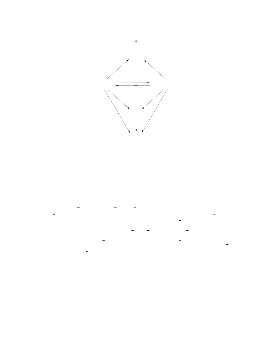
3.1 The Global Realization Theorem for the Reduced Phase Space
28
J
−
1
(
µ
)/
G
µ
L
ϕ
µ
ψ
µ
T(Q/G)
×
Q/G
Q/G
µ
Q/G
µ
Q/G
ρ
µ
σ
µ
σ
µ
p
µ
pr
µ
2
T(Q/G)
Q/G
τ
Q/G
r
µ
pr
µ
1
Figure 3.1:
The maps involved in the proofofthe global realization theorem.
Thus, this condition is equivalent to µ = J
L
(w
q
) + I(q)ξ. Solving for ξ gives the result.
As a consequence, note that for each u
x
∈ T
x
(Q/G), and each q
∈ Q with [q]
G
= x,
there is a v
q
∈ J
−1
L
(µ) such that u
x
= [v
q
].
We claim that an inverse for φ
µ
is the map ψ
µ
: T (Q/G)
×
Q/G
Q/G
µ
→ J
−1
L
(µ)/G
µ
defined by ψ
µ
(u
x
, [q]
G
µ
) = [v
q
]
G
µ
, where x = [q]
G
and u
x
= [v
q
], with v
q
∈ J
−1
L
(µ) given by
the above lemma. To show that ψ
µ
is well-defined, we must show that if we represent the
pair (u
x
, [q]
G
µ
), x = [q]
G
, in a different way, the value of ψ
µ
is unchanged.
Let u
x
= [v
q
], with [q]
G
µ
= [q]
G
µ
and v
q
∈ J
−1
L
(µ). Then we must show that [v
q
]
G
µ
=
[v
q
]
G
µ
. Since [q]
G
µ
= [q]
G
µ
, we can write q = h
·q for some h ∈ G
µ
. Consider h
−1
·v
q
∈ T
q
Q.
By equivariance of J
L
, and the fact that h
∈ G
µ
, we have h
−1
· v
q
∈ J
−1
L
(µ). However,
u
x
= T
q
π
Q,G
(v
q
) = T
q
π
Q,G
(v
q
) = T
q
π
Q,G
(h
−1
· v
q
)
and therefore, v
q
− h
−1
· v
q
∈ g · q. In other words, v
q
− h
−1
· v
q
= ξ
Q
(q) for some ξ
∈ g.
Applying J
L
to each side gives 0 = J
L
(ξ
Q
(q)) = I(q)ξ and so ξ = 0. Thus, v
q
= h
−1
· v
q
and so [v
q
]
G
µ
= [v
q
]
G
µ
. Thus, ψ
µ
is a well defined map.
To show that ψ
µ
is smooth, we show that it has a smooth local representative. If we
write, locally, Q = S
× G where the action is on the second factor alone, then we identify
Q/G
µ
= S
×O
µ
and T (Q/G)
×
Q/G
Q/G
µ
= T S
×O
µ
. We identify J
−1
L
(µ) with T S
×G since
the level set of the momentum map in local representation is given by the product of T S
with the graph of the right invariant vector field on G whose value at e is the vector ζ
∈ g
such that
ζ, η = µ, η. In this representation, J
−1
L
(µ)/G
µ
is identified with T S
× G/G
µ
and the map ψ
µ
is given by (u
x
, [g]
G
µ
)
∈ T S × G/G
µ
→ (u
x
, g
· µ) ∈ T S × O
µ
. This map is
smooth by the construction of the manifold structure on the orbit. Thus, ψ
µ
is smooth.
It remains to show that ψ
µ
and φ
µ
are inverses. To do this, note that
(ψ
µ
◦ φ
µ
)([v
q
]
G
µ
) = ψ
µ
(T
q
π
Q/G
(v
q
), [q]
G
µ
) = [v
q
]
G
µ

3.2 The Routhian.
29
since v
q
is, by assumption, in J
−1
L
(µ).
Associated Bundles.
We now show that the bundle ρ
µ
: Q/G
µ
→ Q/G is globally
diffeomorphic to an associated coadjoint orbit bundle. Let
O
µ
⊂ g
∗
denote the coadjoint
orbit through µ. The associated coadjoint bundle is the bundle
O
µ
= (Q
× O
µ
)/G,
where the action of G on Q is the given (left) action, the action of G on
O
µ
is the left
coadjoint action, and the action of G on Q
× O
µ
is the diagonal action. This coadjoint
bundle is regarded as a bundle over Q/G with the projection map given by ˜
ρ
µ
:
O
µ
→
Q/G; [(q, g
· µ)]
G
→ [q]
G
.
Theorem 3.3. There is a global bundle isomorphism Φ
µ
:
O
µ
→ Q/G
µ
covering the iden-
tity on the base Q/G.
Proof. As in the preceding theorem, we construct the map Φ
µ
and show it is an isomorphism
by constructing an inverse. Define Φ
µ
by [q, g
0
· µ]
G
→ [g
−1
0
· q]
G
µ
. To show that Φ
µ
is well
defined, suppose that g
0
· µ = g · µ and g ∈ G. We have to show that [g
−1
0
· q]
G
µ
=
[
(gg)
−1
· (g · q)]
G
µ
i.e., [g
−1
0
· q]
G
µ
= [g
−1
· q]
G
µ
, which is true because g
−1
0
g
∈ G
µ
. Define
Ψ
µ
: Q/G
µ
→
O
µ
by [q]
G
µ
→ [q, µ]
G
. It is clear that Ψ
µ
is well defined and is the inverse
of Φ
µ
. Smoothness of each of these maps follows from general theorems on smoothness of
quotient maps (see, e.g., Abraham, Marsden and Ratiu [1988]).
A consequence of these two theorems is that there are global bundle isomorphisms be-
tween the three bundles J
−1
L
(µ)/G
µ
, T (Q/G)
×
Q/G
Q/G
µ
, and T (Q/G)
×
Q/G
O
µ
.
The second space is convenient for analyzing the Routhian and the reduced variational
principles, while the third is convenient for making links with the Hamiltonian side.
3.2
The Routhian.
We again consider Lagrangians of the form kinetic minus potential using our earlier notation.
Given a fixed µ
∈ g
∗
, the associated Routhian R
µ
: T Q
→ R is defined by
R
µ
(v
q
) = L(v
q
)
− µ, A(v
q
)
.
Letting A
µ
(v
q
) =
µ, A(v
q
)
, we can write this simply as R
µ
= L
− A
µ
.
Proposition 3.4. For v
q
∈ J
−1
L
(µ), we have R
µ
(v
q
) =
1
2
Hor(v
q
)
2
− V
µ
(q), where the
amended potential V
µ
is given by V
µ
(q) = V (q) + C
µ
(q) and C
µ
=
1
2
µ, I(q)
−1
µ
is
called the amendment.
Proof. Because the horizontal and vertical components in the mechanical connection are
metrically orthogonal, we have
R
µ
(v
q
) =
1
2
v
q
2
− V (q) − µ, A(v
q
)
=
1
2
Hor(v
q
)
2
+
1
2
Ver(v
q
)
2
− V (q) − µ, A(v
q
)
.
For v
q
∈ J
−1
L
(µ), we have
Ver(v
q
)
2
=
(A(v
q
))
Q
(q)
2
=
I(q)A(v
q
), A(v
q
)
=
J
L
(v
q
), A(v
q
)
= µ, A(v
q
)
=
µ, I(q)
−1
(µ)
.

3.3 Examples
30
Using this, one now verifies the following:
Proposition 3.5. The function R
µ
is G
µ
-invariant and so it induces, by restriction and
quotienting, a function on J
−1
L
(µ)/G
µ
and hence, by the global realization theorem, a func-
tion R
µ
: T (Q/G)
×
Q/G
(Q/G
µ
)
→ R called the reduced Routhian; it is given by
R
µ
(u
x
, [q]
G
µ
) =
1
2
u
x
2
S
− V
µ
([q]
G
µ
),
where x = [q]
G
, the metric on S = Q/G is naturally induced from the metric on Q (that
is, if u
x
= T
q
π
Q,G
(v
q
) then
u
x
S
=
Hor(v
q
)
), and V
µ
: Q/G
µ
→ R is the reduced
amended potential given by V
µ
([q]
G
µ
) = V
µ
(q).
Additional notation will prove useful. Let V be the function on Q/G induced by the
function V on Q and let C
µ
be the reduced amendment, the function on Q/G
µ
induced
by the amendment C
µ
. Thus, V
µ
= V
◦ ρ
µ
+ C
µ
. Let the Lagrangian on Q/G be denoted
L = K
− V, where K(u
x
) =
u
x
2
S
/2 is the kinetic energy on the shape space Q/G.
3.3
Examples
Rigid Body.
Here the shape space is a point since Q = G, µ = π, the spatial angular
momentum, so T (Q/G)
×
Q/G
Q/G
π
= S
2
π
, the sphere of radius
π, a coadjoint orbit for
the rotation group. The reduced Routhian R
π
: S
2
π
→ R is the negative of the reduced
amendment, namely
−
1
2
Π
· I
−1
Π. This is of course the negative of the reduced energy.
Heavy Top.
In this case Q = SO(3) and G = S
1
is the subgroup of rotations about the
vertical axis. Shape space is Q/G = S
2
1
, the sphere of radius 1. As with any Abelian group,
G
µ
= G, so T (Q/G)
×
Q/G
Q/G
µ
= T (Q/G). In the case of the heavy top, we get T S
2
1
.
The isomorphism from J
−1
L
(µ)/G
µ
→ T S
2
is induced by the map that takes (A, ˙
A) to
(Γ, ˙
Γ = Γ
× Ω). One checks that the horizontal lift of (Γ, ˙Γ) to the point A is the vector
(A, ˙
A
h
) satisfying A
−1
˙
A
h
= Ω
h
, where
Ω
h
:= ˙
Γ
× Γ −
( ˙
Γ
× Γ) · IΓ
Γ
· IΓ
Γ.
In doing this computation, it may be helpful to keep in mind that the condition of horizon-
tality is the same as zero momentum. Thus, the reduced Routhian is given by
R
µ
(Γ, ˙
Γ) =
1
2
Ω
h
, IΩ
h
− MglΓ · χ −
1
2
µ
2
Γ
· IΓ
.
Underwater Vehicle.
As we have seen, Q = SE(3), G = SE(2)
× R and so again Q/G =
S
2
1
. However, because G is nonabelian, for µ
= 0, the bundle Q/G
µ
→ Q/G has nontrivial
fibers. These fibers are coadjoint orbits for SE(2), namely cylinders. A computation shows
that Q/G
µ
= SO(3)
× R, regarded as a bundle over S
2
1
by sending (A, λ) to A
−1
k. Thus,
T (Q/G)
×
Q/G
Q/G
µ
= T (S
2
1
)
×
S
2
1
SO(3)
×R, a 6-dimensional space, a nontrivial bundle over
the two sphere with fiber the product of the tangent space to the sphere with a cylinder. The
reduced Routhian may be computed as in the previous example, but we omit the details.
3.4
Hamilton’s Variational Principle and the Routhian
Now we shall recast Hamilton’s principle for the Lagrangian L in terms of the Routhian.
To do so, we shall first work out the expression for dS
R
µ
.

3.4 Hamilton’s Variational Principle and the Routhian
31
Recalling that R
µ
= L
− A
µ
and that on the space of curves parametrized on a fixed
interval [a, b], S
L
(q(
·)) =
b
a
L(q(t), ˙q(t)) dt, we see that S
R
µ
= S
L
− S
A
µ
, and hence that
dS
R
µ
· δq(t) = dS
L
· δq(t) − dS
A
µ
· δq(t).
(3.1)
We know from the formula for dS
L
given in Proposition 1.1 that
dS
L
q(t)
· δq(t) =
b
a
EL(L)
d
2
q
dt
2
· δq dt + Θ
L
dq
dt
·
δq
b
a
.
(3.2)
To work out the term dS
A
µ
· δq(t) we shall proceed in a more geometric way.
Variations of Integrals of Forms.
We shall pause for a moment to consider the general
question of variations of the integrals of differential forms. Consider a manifold M , a k-
dimensional compact oriented submanifold S (with boundary) and a k-form ω defined on
M . By a variation of S we shall mean a vector field δs defined along S in the following
way. Let ϕ
: M
→ M be a family of diffeomorphisms of M with ϕ
0
the identity. Set
δs(m) =
∂
∂*
=0
ϕ
(m)
and
δ
S
ω =
∂
∂*
=0
ϕ
(S)
ω.
Proposition 3.6. The above variation is given by
δ
S
ω =
S
i
δs
dω +
∂S
i
δs
ω,
where i
δs
ω denotes the interior product of the vector field δs with the k-form ω.
Proof. We use the definition, the change of variables formula, the Lie derivative and Stokes’
formula as follows:
δ
S
ω =
∂
∂*
=0
ϕ
(S)
ω =
∂
∂*
=0
S
ϕ
∗
ω
=
S
£
δs
ω =
S
i
δs
dω +
S
di
δs
ω =
S
i
δs
dω +
∂S
i
δs
ω.
Application to the Mechanical Connection.
In particular, we can apply the preceding
proposition to the variations of the integral of the one form A
µ
over curves. We get
δ
b
a
A
µ
=
b
a
i
δq
B
µ
+ A
µ
(δq(b))
− A
µ
(δq(a)),
where B
µ
= dA
µ
, the exterior derivative of the one form A
µ
.
The Computation of Boundary Terms.
Summing up what we have proved so far, we
write
dS
R
µ
(q(t), ˙q(t))
· δq = dS
L
(q(t), ˙q(t))
· δq − dS
A
µ
(q(t), ˙q(t))
· δq
=
b
a
EL(L)
d
2
q
dt
2
· δq dt + Θ
L
dq
dt
·
δq
b
a
−
b
a
i
δq
B
µ
− [A
µ
(δq(b))
− A
µ
(δq(a))] .
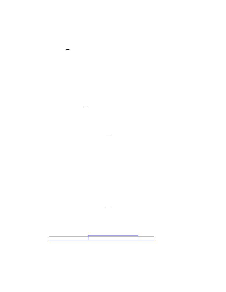
3.4 Hamilton’s Variational Principle and the Routhian
32
We now compute the boundary terms in this expression. Recalling the formula for the
boundary terms in the variational formula for L, splitting the variation into horizontal and
vertical parts, we get
Θ
L
dq
dt
·
δq
b
a
=
FL(q(t), ˙q(t)), δq|
b
a
=
FL(q(t), ˙q(t)), Hor δq|
b
a
+
FL(q(t), ˙q(t)), Ver δq|
b
a
=
˙q(t), Hor δq|
b
a
+
˙q(t), Ver δq|
b
a
.
Assuming the curve (q(t), ˙q(t)) lies in the level set of the momentum map, we have
˙q(t), Ver δq =
˙q(t), [A(δq)]
Q
(q)
=
J
L
(q(t), ˙q(t)), A(δq)
= µ, A(δq) = A
µ
(δq)
Therefore, we get
Θ
L
dq
dt
·
δq
b
a
=
˙q(t), Hor δq|
b
a
+ A
µ
(δq)
|
b
a
.
Noticing that the terms involving A
µ
cancel, we can say, in summary, that
dS
R
µ
(q(t), ˙q(t))
· δq = dS
L
(q(t), ˙q(t))
· δq − dS
A
µ
(q(t), ˙q(t))
· δq
=
b
a
EL(L)
d
2
q
dt
2
· δq dt −
b
a
i
δq
B
µ
+
˙q(t), Hor δq|
b
a
.
We can conclude the following.
Theorem 3.7. A solution of the Euler–Lagrange equations which lies in the level set J
L
=
µ, satisfies the following variational principle
δ
b
a
R
µ
(q(t), ˙q(t)) dt =
−
b
a
i
δq
B
µ
(q(t), ˙q(t)) dt +
˙q(t), Hor δq|
b
a
.
It is very important to notice that in this formulation, there are no boundary conditions
or constraints whatsoever imposed on the variations. However, we can choose vanishing
boundary conditions for δq and derive:
Corollary 3.8. Any solution of the Euler–Lagrange equations which lies in the level set
J
L
= µ, also satisfies the equations
EL(R
µ
)
d
2
q
dt
2
(t)
= i
˙
q(t)
B
µ
.
Conversely, any solution of these equations that lies in the level set J
L
= µ of the momentum
map is a solution to the Euler–Lagrange equations for L.
In deriving these equations, we have interchanged the contractions with δq and ˙q using
skew symmetry of the two form B
µ
. One can also check this result with a coordinate
computation, as was done in Marsden and Scheurle [1993b]; see also Marsden and Ratiu
[1999] for this calculation in the case of Abelian groups.
3.5 The Routh VariationalPrinciple on Quotients
33
3.5
The Routh Variational Principle on Quotients
We now show how to drop the variational principle given in the preceding subsection to
the reduced space T (Q/G)
×
Q/G
Q/G
µ
. An important point is whether or not one imposes
constraints on the variations in the variational principle. One of our main points is that such
constraints are not needed; for a corresponding derivation with the varied curves constrained
to lie in the level set of the momentum map, see Jalnapurkar and Marsden [2000a].
Later in this section we illustrate the procedure with the rigid body, which already
contains the key to how one relaxes the constraints. Some readers may find it convenient
to study that example simultaneously with the general theory.
Our first goal is to show that the variation of the Routhian evaluated at a solution
depends only on the quotient variations. Following this, we shall show that the gyroscopic
terms i
˙
q(t)
B
µ
also depend only on the quotient variations.
Analysis of the Variation of the Routhian.
We begin by writing the Routhian as
follows:
R
µ
(v
q
) =
1
2
Hor(v
q
)
2
+
1
2
Ver(v
q
)
2
− V (q) − µ, A(v
q
)
.
(3.3)
We next analyze the variation of two of the terms in this expression, namely
1
2
Ver(v
q
)
2
− µ, A(v
q
)
=
1
2
I(q)A(v
q
), A(v
q
)
− µ, A(v
q
)
.
We choose a family of curves q(t, *) with the property that q(t, 0) is a solution of the Euler–
Lagrange equations with a momentum value µ and let v
q
be the time derivative of q(t, 0).
As usual, we also let δq be the * derivative evaluated at * = 0. Then, the desired variation
is given by
∂
∂*
=0
1
2
I(q)A
∂q
∂t
, A
∂q
∂t
−
µ, A
∂q
∂t
=
1
2
(T
q
I
· δq) A(v
q
), A(v
q
)
+
I(q)A(v
q
)
− µ,
∂
∂*
=0
A
∂q
∂t
.
(3.4)
Here, T
q
denotes the tangent map at the point q. Since the curve q(t, 0) is assumed to be
a solution with momentum value µ and since I(q)A(v
q
) = J
L
(v
q
), the second term in the
preceding display vanishes. Thus, we conclude that
∂
∂*
=0
1
2
I(q)A
∂q
∂t
, A
∂q
∂t
−
µ, A
∂q
∂t
=
1
2
(T
q
I
· δq) A(v
q
), A(v
q
)
(3.5)
Next, we observe that
d
1
2
µ, I(q)
−1
µ
· δq = −
1
2
µ, I(q)
−1
(T
q
I
· δq) I(q)
−1
µ
.
(3.6)
On a solution with momentum value µ, we have µ = J
L
(v
q
) = I(q)A(v
q
). Substituting this
into the preceding expression, we get
d
1
2
µ, I(q)
−1
µ
· δq = −
1
2
I(q)A(v
q
), I(q)
−1
(T
q
I
· δq) I(q)
−1
I(q)A(v
q
)
=
−
1
2
(T
q
I
· δq) A(v
q
), A(v
q
)
.
(3.7)
3.5 The Routh VariationalPrinciple on Quotients
34
Therefore, on a solution with momentum value µ, we have
∂
∂*
=0
1
2
I(q)A
∂q
∂t
, A
∂q
∂t
−
µ, A
∂q
∂t
(3.8)
=
−d
1
2
µ, I(q)
−1
µ
· δq.
(3.9)
We conclude that when evaluated on a solution with momentum value µ,
∂
∂*
=0
R
µ
∂q
∂t
=
∂
∂*
=0
1
2
Hor
∂q
∂t
2
− V
µ
(q)
=
∂
∂*
=0
R
µ
∂q
∂t
,
(3.10)
where R
µ
(v
q
) =
1
2
Hor(v
q
)
2
− V
µ
(q). Proposition 3.4 shows that R
µ
agrees with R
µ
on
J
−1
L
(µ) and, more importantly, R
µ
= R
µ
◦
T π
Q,G
×
Q/G
π
Q,G
µ
, where, recall, π
Q,G
: Q
→
Q/G and π
Q,G
µ
: Q
→ Q/G
µ
are the projection maps. Thus, R
µ
drops to the quotient
with no restriction to the level set of the momentum map. Differentiating this relation with
respect to *, it follows that the variation of R
µ
drops to the variation of R
µ
.
Analysis of the Variation of the Gyroscopic Terms.
Now we shall show how the
exterior derivative of the one form A
µ
drops to the quotient space. Precisely, this means the
following. We consider the one form A
µ
on the space Q and its exterior derivative B
µ
= dA
µ
.
We claim that there is a unique two form β
µ
on Q/G
µ
such that B
µ
= π
∗
Q,G
µ
β
µ
, where,
recall, π
Q,G
µ
: Q
→ Q/G
µ
is the natural projection. To prove this, one must show that for
any u, v
∈ T
q
Q, the following identity holds:
dA
µ
(q)(u, v) = dA
µ
(g
· q) (g · u + ξ
Q
(g
· q), g · v + η
Q
(g
· q)) ,
(3.11)
for any g
∈ G
µ
, and ξ, η
∈ g
µ
. To prove this, one first shows that
dA
µ
(g
· q) (g · u + ξ
Q
(g
· q), g · v + η
Q
(g
· q))
= dA
µ
(q)
u +
Ad
g
−1
ξ
Q
(q), v +
Ad
g
−1
η
Q
(q)
using the identities ξ
Q
(g
· q) =
Ad
g
−1
ξ
Q
(q) and Φ
∗
g
A
µ
= A
µ
, where Φ
g
(q) = g
· q is the
group action. Second, one shows that dA
µ
(q) (u + ζ
Q
(q), v) = dA
µ
(q) (u, v) for any ζ
∈ g
µ
.
This holds because i
ζ
Q
dA
µ
= 0. Indeed, from Φ
∗
g
A
µ
= A
µ
we get £
ζ
Q
A
µ
= 0 and hence
i
ζ
Q
dA
µ
+ di
ζ
Q
A
µ
= 0. However, i
ζ
Q
A
µ
=
µ, ζ, a constant, so we get the desired result.
Now we can apply Theorem 3.7 to obtain the following result.
Theorem 3.9. If q(t), a
≤ t ≤ b is a solution of the Euler–Lagrange equations with mo-
mentum value µ, y(t) = π
Q,G
µ
(q(t)), and x(t) = π
Q,G
(q(t)), then y(t) satisfies the reduced
variational principle
δ
b
a
R
µ
(x(t), ˙x(t), y(t)) dt =
b
a
i
˙
y(t)
β
µ
(y(t))
· δy dt + ˙x(t), δx(t)
S
|
b
a
.
Conversely, if q(t) is a curve such that ˙q(t)
∈ J
−1
L
(µ) and if its projection to y(t) satisfies
this reduced variational principle, then q(t) is a solution of the Euler–Lagrange equations.
It is already clear from the case of the Euler–Poincar´e equations that dropping the varia-
tional principle to the quotient can often be easier than dropping the equations themselves.
Notice also that there is a slight abuse of notation, similar to that when one writes a tangent
vector as a pair (q, ˙q). The notation (x, y) is redundant since x can be recovered from y by
projection from Q/G
µ
to Q/G. Consistent with this convenient notational abuse, we use
the notation (x, ˙x) is an alternative to u
x
.

3.6 Curvature
35
3.6
Curvature
We pause briefly to recall some key facts about curvatures of connections, and establish our
conventions. Then we shall relate β
µ
to curvature.
Review of the Curvature of a Principal Connection.
Consider a principal connection
A on a principal G bundle π
Q,G
: Q
→ Q/G. The curvature B is the Lie algebra-valued
two-form on Q defined by
B(u
q
, v
q
) = d
A(Hor
q
(u
q
), Hor
q
(v
q
)), where d is the exterior
derivative.
Using the fact that
B depends only on the horizontal part of the vectors and equivariance,
one shows that it defines an adjoint bundle (that is, ˜
g)-valued two-form on the base Q/G
by Curv
A
(x)(u
x
, v
x
) = [q, d
A(u
q
, v
q
)]
G
, where [q]
G
= x
∈ Q/G, u
q
and v
q
are horizontal,
T π
Q,G
· u
q
= u
x
and T π
Q,G
· v
q
= v
x
.
Curvature measures the lack of integrability of the horizontal distribution in the sense
that on two vector fields u, v on Q one has
B(u, v) = −A([Hor(u), Hor(v)]).
The proof uses the Cartan formula relating the exterior derivative and the Jacobi-Lie
bracket:
B(u, v) = Hor(u)[A(Hor(v))] − Hor(v)[A(Hor(u))] − A([Hor(u), Hor(v)]).
The first two terms vanish since
A vanishes on horizontal vectors.
An important formula for the curvature of a principal connection is given by the Cartan
structure equations: for any vector fields u, v on Q one has
B(u, v) = dA(u, v) − [A(u), A(v)],
where the bracket on the right hand side is the Lie bracket in g. One writes this equation for
short as
B = dA − [A, A]. An important consequence of these equations that we will need
below is the following identity (often this is a lemma used to prove the structure equations):
d
A(q) (Hor u
q
, Ver v
q
) = 0
(3.12)
for any u
q
, v
q
∈ T
q
Q.
Recall also that when applied to the left trivializing connection on a Lie group, the
structure equations reduce to the Mauer–Cartan Equations. We also remark, although we
shall not need it, that one has the Bianchi Identities: for any vector fields u, v, w on Q,
we have
d
B(Hor(u), Hor(v), Hor(w)) = 0.
The Connection on the Bundle ρ
µ
.
The bundle ρ
µ
: Q/G
µ
→ Q/G has an Ehresmann
connection induced from the principal connections on the two bundles Q
→ Q/G
µ
and
Q
→ Q/G. However, we can also determine this connection directly by giving its horizontal
space at each point y = [q]
G
µ
∈ Q/G
µ
. This horizontal space is taken to be the orthogonal
complement within T
y
(Q/G
µ
) ∼
= T
q
Q/[g
µ
· q] to the vertical space [g · q]/[g
µ
· q]. This latter
space inherits its metric from that on T
q
Q by taking the quotient metric. As before, since
the action is by isometries, this metric is independent of the representatives chosen.
This horizontal space is denoted by Hor
ρ
µ
and the operation of taking the horizontal part
of a vector is denoted by the same symbol. The vertical space is of course the fiber of this
bundle. This vertical space at a point y = [q]
G
µ
is given by ker T
y
ρ
µ
, which is isomorphic

3.6 Curvature
36
to the quotient space [g
· q]/[g
µ
· q]. This vertical bundle will be denoted by Ver(Q/G
µ
)
⊂
T (Q/G
µ
) and the fiber at the point y
∈ Q/G
µ
is denoted Ver
y
(Q/G
µ
) = ker T
y
ρ
µ
. The
projection onto the vertical part defines the analogue of the connection form, which we
denote A
ρ
µ
. Thus, A
ρ
µ
: T (Q/G
µ
)
→ Ver(Q/G
µ
), which we think of as a vertical valued
one form.
Compatibility of the Three Connections.
We shall now work towards the computa-
tion of β
µ
on various combinations of horizontal and vertical vectors relative to the connec-
tion A
ρ
µ
. To do this, keep in mind that ρ
µ
◦ π
Q,G
µ
= π
Q,G
by construction. We shall need
the following.
Lemma 3.10. Let u
q
∈ T
q
Q and u
y
= T
y
π
Q,G
µ
· u
q
, where y = π
Q,G
µ
(q). Then
1. u
y
is ρ
µ
-vertical if and only if u
q
is π
Q,G
-vertical.
2. The identity T π
Q,G
µ
· Hor u
q
= Hor
ρ
µ
(u
y
) holds, where Hor denotes the horizontal
projection for the mechanical connection A.
3. The following identity holds: T π
Q,G
µ
· Ver u
q
= V er
ρ
µ
(u
y
) .
Proof. 1. Because ρ
µ
◦ π
Q,G
µ
= π
Q,G
, the chain rule gives
T
y
ρ
µ
· u
y
= T
y
ρ
µ
· T
q
π
Q,G
µ
· u
q
= T
q
π
Q,G
· u
q
,
so T
y
ρ
µ
· u
y
= 0 if and only if T
q
π
Q,G
· u
q
= 0, which is the statement of part 1.
2. Let v
y
∈ ker T
y
ρ
µ
⊂ T
y
(Q/G
µ
) and write v
y
= T
q
π
Q,G
µ
· v
q
. By the definition of the
metric
·, ·
Q/G
µ
on Q/G
µ
we have
0 =
Hor u
q
, v
q
Q
=
T
q
π
Q,G
µ
· Hor u
q
, T
q
π
Q,G
µ
· v
q
Q/G
µ
=
T
q
π
Q,G
µ
· Hor u
q
, v
y
Q/G
µ
.
Hence, since v
y
is an arbitrary ρ
µ
-vertical vector, we conclude that T
q
π
Q,G
µ
· Hor u
q
is
ρ
µ
-horizontal. Next, write
Hor
ρ
µ
T π
Q,G
µ
· u
q
= Hor
ρ
µ
T π
Q,G
µ
· Hor u
q
+ Hor
ρ
µ
T π
Q,G
µ
· Ver u
q
= T π
Q,G
µ
· Hor u
q
by assertion 1 of this lemma.
3. As in 1, T
q
π
Q,G
µ
· Ver u
q
is ρ
µ
-vertical. Therefore,
Ver
ρ
µ
u
y
= V er
ρ
µ
T
q
π
Q,G
µ
· u
q
= V er
ρ
µ
T
q
π
Q,G
µ
· Ver u
q
+ V er
ρ
µ
T
q
π
Q,G
µ
· Hor u
q
= T
q
π
Q,G
µ
· Ver u
q
,
since T
q
π
Q,G
µ
· Hor u
q
is ρ
µ
-horizontal by part 2.
The Pairing Between ˜
g and ˜
g
∗
.
We shall need to define a natural pairing between the
adjoint and coadjoint bundles. Recall that, by definition, ˜
g = (Q
×g)/G and ˜g
∗
= (Q
×g
∗
)/G,
where G acts by the given action on Q and by the adjoint action on g and the coadjoint
action on g
∗
. For [q, µ]
G
∈ ˜g
∗
and [q, ξ]
G
∈ ˜g, the pairing is [q, µ]
G
, [q, ξ]
G
= µ, ξ . One
shows that this pairing is independent of the representatives chosen.
We define, for y = [q]
G
µ
∈ Q/G
µ
, the (y, µ)-component of Curv
A
by
Curv
(y,µ)
A
(x)(u
x
, v
x
) =
[q, µ]
G
, Curv
A
(x)(u
x
, v
x
)
(3.13)
where [q]
G
= x. One shows that this is independent of the representative q chosen for y.
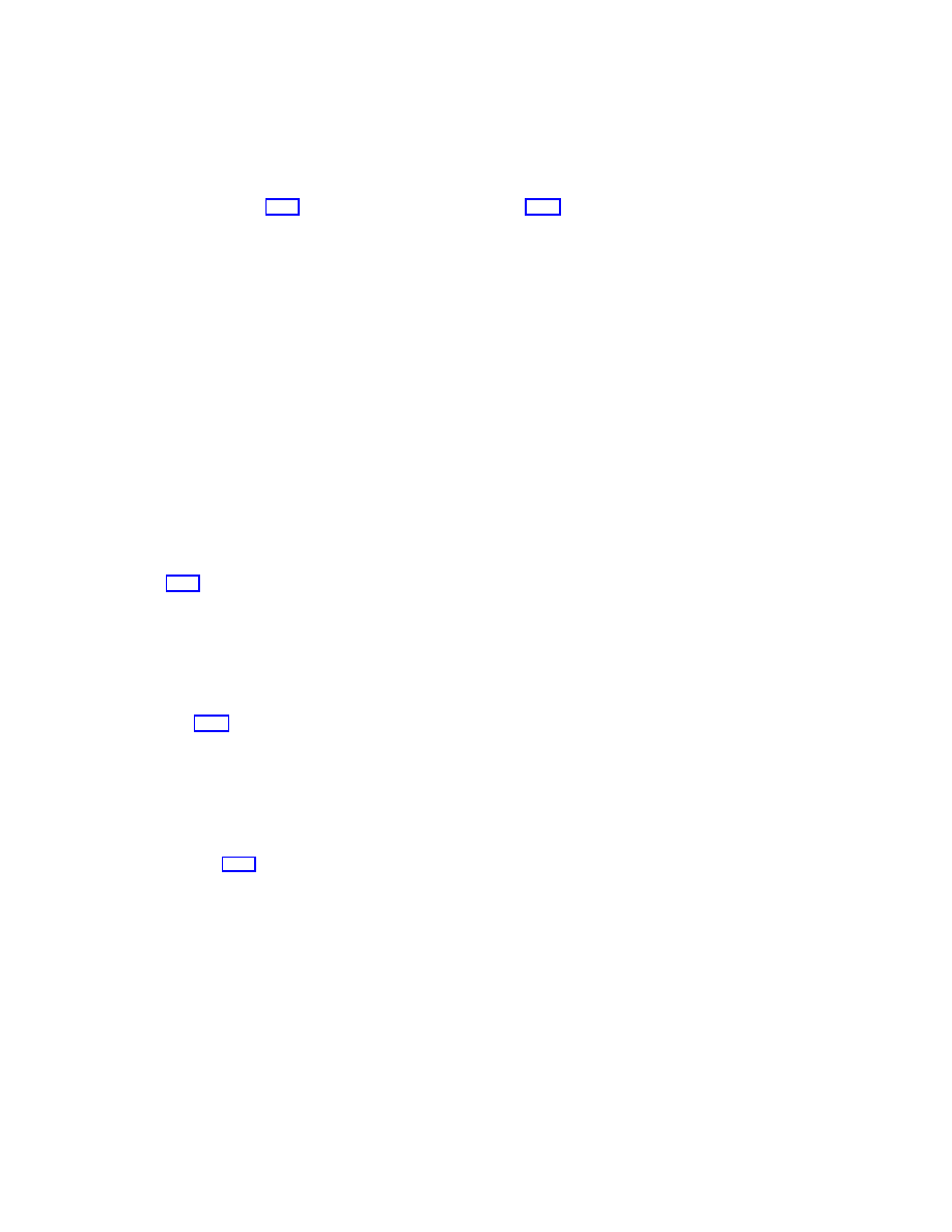
3.6 Curvature
37
Hor-Hor Components of β
µ
.
Now we compute the horizontal-horizontal components
of β
µ
as follows. Let u
q
, v
q
∈ T
q
Q, and
u
y
= T
q
π
Q,G
µ
· u
q
,
v
y
= T
q
π
Q,G
µ
· v
q
.
Using Lemma 3.10, the definition of curvature, and (3.13), we have
β
µ
(y)(Hor
ρ
µ
u
y
, Hor
ρ
µ
v
y
) = β
µ
(π
Q,G
µ
(q))(T
q
π
Q,G
µ
· Hor u
q
, T
q
π
Q,G
µ
· Hor v
q
)
=
π
∗
Q,G
µ
β
µ
(q) (Hor u
q
, Hor v
q
)
= B
µ
(q) (Hor u
q
, Hor v
q
)
=
µ, dA(q) (Hor u
q
, Hor v
q
)
=
[q, µ]
G
, [q, dA(q) (Hor u
q
, Hor v
q
)]
G
=
[q, µ]
G
, Curv
A
(x)(u
x
, v
x
)
= Curv
(y,µ)
A
(x) (u
x
, v
x
) ,
where x = π
Q,G
(q) = ρ
µ
(y), u
x
= T
q
π
Q,G
· u
q
= T
y
ρ
µ
· u
y
, and similarly for v
x
.
We summarize what we have proved in the following lemma.
Lemma 3.11. The two form β
µ
on horizontal vectors is given by
β
µ
(y)(Hor
ρ
µ
u
y
, Hor
ρ
µ
v
y
) = Curv
(y,µ)
A
(x) (u
x
, v
x
) .
(3.14)
Hor-Ver Components of β
µ
.
Now we compute the horizontal-vertical components of
β
µ
as follows. Let u
q
, v
q
∈ T
q
Q, and u
y
= T
q
π
Q,G
µ
· u
q
, v
y
= T
q
π
Q,G
µ
· v
q
. Using Lemma
3.10, we have
β
µ
(y)(Hor
ρ
µ
u
y
, Ver
ρ
µ
v
y
) = β
µ
(π
Q,G
µ
(q))(T
q
π
Q,G
µ
· Hor u
q
, T
q
π
Q,G
µ
· Ver v
q
)
=
π
∗
Q,G
µ
β
µ
(q) (Hor u
q
, Ver v
q
)
= B
µ
(q) (Hor u
q
, Ver v
q
)
=
µ, dA(q) (Hor u
q
, Ver v
q
)
= 0,
by (3.12). We summarize what we have proved in the following lemma.
Lemma 3.12. The two form β
µ
on pairs of horizontal and vertical vectors vanishes:
β
µ
(y)(Hor
ρ
µ
u
y
, Ver
ρ
µ
v
y
) = 0.
(3.15)
Ver-Ver Components of β
µ
.
Now we compute the vertical-vertical components of β
µ
as follows. As above, let u
q
, v
q
∈ T
q
Q, and u
y
= T
q
π
Q,G
µ
· u
q
, v
y
= T
q
π
Q,G
µ
· v
q
. Using
Lemma 3.10, we have
β
µ
(y)(Ver
ρ
µ
u
y
, Ver
ρ
µ
v
y
) = β
µ
(π
Q,G
µ
(q))(T
q
π
Q,G
µ
· Ver u
q
, T
q
π
Q,G
µ
· Ver v
q
)
=
π
∗
Q,G
µ
β
µ
(q) (V er u
q
, Ver v
q
)
= B
µ
(q) (V er u
q
, Ver v
q
)
=
µ, dA(q) (V er u
q
, Ver v
q
)
=
µ, [A(q) V er u
q
, A(q) V er v
q
]
by the Cartan structure equations. We now write
Ver u
q
= ξ
Q
(q)
and
Ver v
q
= η
Q
(q),

3.7 Splitting the Reduced Variational Principle
38
so that the preceding equation becomes:
β
µ
(y)(Ver
ρ
µ
u
y
, Ver
ρ
µ
v
y
) =
µ, [ξ, η]
(3.16)
Now given Ver
ρ
µ
u
y
∈ ker T
y
ρ
µ
, we can represent it as a class [ξ
Q
(q)]
∈ g · q/g
µ
· q. The map
ξ
→ ξ
Q
(q) induces an isomorphism of g/g
µ
with the ρ
µ
-vertical space. Note that the above
formula depends only on the class of ξ and of η.
We summarize what we have proved in the following lemma.
Lemma 3.13. The two form β
µ
on pairs of vertical vectors is given by the following formula
β
µ
(y)(Ver
ρ
µ
u
y
, Ver
ρ
µ
v
y
) =
µ, [ξ, η] ,
(3.17)
where Ver
ρ
µ
u
y
= [ξ
Q
(q)] and Ver
ρ
µ
v
y
= [η
Q
(q)].
3.7
Splitting the Reduced Variational Principle
Now we want to take the reduced variational principle, namely
δ
b
a
R
µ
(x(t), ˙x(t), y(t)) dt =
b
a
i
˙
y(t)
β
µ
(y(t))
· δy dt + ˙x(t), δx(t)|
b
a
and relate it intrinsically to two sets of differential equations corresponding to the horizontal
and vertical components of the bundle ρ
µ
: Q/G
µ
→ Q/G.
Recall that in this principle, we are considering all curves y(t)
∈ Q/G
µ
and x(t) =
ρ
µ
(y(t))
∈ Q/G. For purposes of deriving the equations, we can restrict to variations such
that δx vanishes at the endpoints, so that the boundary term disappears.
Now the strategy is to split the variations δy(t) of y(t) into horizontal and vertical
components relative to the induced connection on the bundle ρ
µ
: Q/G
µ
→ Q/G.
Breaking Up the Variational Principle.
Now we can break up the variational principle
by decomposing variations into their horizontal and vertical pieces, which we shall write
δy = Hor
ρ
µ
δy + V er
ρ
µ
δy,
where
A
ρ
µ
δy = V er
ρ
µ
δy.
We also note that, by construction, the map T ρ
µ
takes δy to δx. Since this map has kernel
given by the set of vertical vectors, it defines an isomorphism on the horizontal space to the
tangent space to shape space. Thus, we can identify Hor
ρ
µ
δy with δx.
Horizontal Variations.
Now we take variations that are purely horizontal and vanish at
the endpoints; that is, δy = Hor
ρ
µ
δy. In this case, the variational principle,
δ
b
a
R
µ
(x(t), ˙x(t), y(t)) dt =
b
a
i
˙
y(t)
β
µ
(y(t))
· δy dt + ˙x(t), δx(t)|
b
a
(3.18)
becomes
δ
b
a
[L(x(t), ˙x(t))
− C
µ
(y(t))] dt
· Hor
ρ
µ
δy(t) =
b
a
i
˙
y(t)
β
µ
(y(t))
· Hor
ρ
µ
δy(t) dt. (3.19)
Since, by our general variational formula, for variations vanishing at the endpoints,
δ
b
a
L(x(t), ˙
x(t)) dt
· δx =
b
a
EL(L)(x(t), ˙x(t), ¨x(t)) · δx(t) dt,
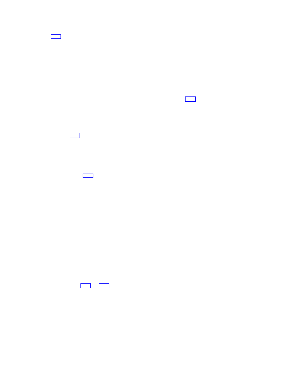
3.8 The Lagrange–Routh Equations
39
(3.19) is equivalent to
EL(L)(¨x) = Hor
ρ
µ
dC
µ
(y) + i
˙
y(t)
β
µ
(y(t))
(3.20)
where, for a point γ
∈ T
∗
y
(Q/G
µ
), we define
Hor
ρ
µ
γ
∈ T
∗
x
(Q/G)
by
Hor
ρ
µ
γ
(T
y
ρ
µ
· δy) = γ(Hor
ρ
µ
δy).
This is well defined because the kernel of T
y
ρ
µ
consists of vertical vectors and these are
annihilated by the map Hor
ρ
µ
.
Vertical Variations.
Now we consider vertical variations; that is, we take variations
δy(t) = V er
ρ
µ
δy(t). The left hand side of the variational principle (3.18) now becomes
δ
b
a
R
µ
(x(t), ˙x(t), y(t)) dt = δ
b
a
[
−C
µ
(y(t))] dt =
b
a
−dC
µ
(y(t))
· Ver
ρ
µ
δy(t)
dt
As before, the right hand side is
b
a
i
˙
y(t)
β
µ
(y(t))
· Ver
ρ
µ
δy(t) dt. Hence, the variational
principle (3.18) gives
Ver
ρ
µ
dC
µ
(y) + i
˙
y(t)
β
µ
(y(t))
= 0
(3.21)
where, for a point γ
∈ T
∗
y
(Q/G
µ
), we define
Ver
ρ
µ
γ
∈ Ver
∗
y
(Q/G
µ
)
by
Ver
ρ
µ
γ
= γ
| Ver
y
(Q/G
µ
).
We can rewrite (3.21) to isolate Ver
ρ
µ
˙y as follows
Ver
ρ
µ
i
Ver
ρµ
˙
y
β
µ
(y)
=
− Ver
ρ
µ
dC
µ
(y) + i
Hor
ρµ
˙
y(t)
β
µ
(y(t))
.
(3.22)
3.8
The Lagrange–Routh Equations
We now put together the information on the structure of the two form β
µ
with the reduced
equations in the previous section.
The Horizontal Equation.
We begin with the horizontal reduced equation:
EL(L)(¨x) = Hor
ρ
µ
dC
µ
(y) + i
˙
y(t)
β
µ
(y(t))
(3.23)
We now compute the term Hor
ρ
µ
i
˙
y(t)
β
µ
(y(t)). To do this, let δx
∈ T
x
(Q/G) and write
δx = T
y
ρ
µ
· δy. By definition,
Hor
ρ
µ
i
˙
y(t)
β
µ
(y(t)), δx
(3.24)
=
i
˙
y(t)
β
µ
(y(t)), Hor
ρ
µ
δy
= β
µ
(y(t))
˙y(t), Hor
ρ
µ
δy
= β
µ
(y(t))
Hor
ρ
µ
˙y(t), Hor
ρ
µ
δy
+ β
µ
(y(t))
Ver
ρ
µ
˙y(t), Hor
ρ
µ
δy
Using Lemmas 3.11 and 3.12, this becomes
Hor
ρ
µ
i
˙
y(t)
β
µ
(y(t)), δx
(3.25)
= Curv
(y(t),µ)
A
(x(t))
T
y(t)
ρ
µ
·
Hor
ρ
µ
˙y(t)
, T
y(t)
ρ
µ
·
Hor
ρ
µ
δy
= Curv
(y(t),µ)
A
(x(t))
T
y(t)
ρ
µ
·
Hor
ρ
µ
˙y(t)
, T
y(t)
ρ
µ
· δy
,
(3.26)
3.8 The Lagrange–Routh Equations
40
since T
y(t)
ρ
µ
annihilates the vertical component of δy. Next, we claim that
T
y(t)
ρ
µ
·
Hor
ρ
µ
˙y(t)
= ˙x(t)
(3.27)
To see this, we start with the definition of x(t) = ρ
µ
(y(t)) and use the chain rule to get
˙x(t) = T
y(t)
ρ
µ
· ˙y(t) = T
y(t)
ρ
µ
·
Hor
ρ
µ
˙y(t)
since T
y
ρ
µ
vanishes on ρ
µ
-vertical vectors. This
proves the claim. Substituting (3.27) into (3.26) and using δx = T
y
ρ
µ
· δy, we get
Hor
ρ
µ
i
˙
y(t)
β
µ
(y(t)), δx
= Curv
(y(t),µ)
A
(x(t)) ( ˙x(t), δx)
(3.28)
Therefore,
Hor
ρ
µ
i
˙
y(t)
β
µ
(y(t)) = i
˙
x(t)
Curv
(y(t),µ)
A
(x(t)).
(3.29)
Thus, (3.23) becomes
EL(L)(¨x) = i
˙
x(t)
Curv
(y(t),µ)
A
(x(t)) + Hor
ρ
µ
dC
µ
(y).
(3.30)
The Vertical Equation.
Now we analyze in a similar manner, the vertical equation. We
start with
Ver
ρ
µ
i
Ver
ρµ
˙
y
β
µ
(y)
=
− Ver
ρ
µ
dC
µ
(y) + i
Hor
ρµ
˙
y(t)
β
µ
(y(t))
.
(3.31)
We pair the left hand side with a vertical vector, Ver
ρ
µ
δy and use the definitions to get
Ver
ρ
µ
i
Ver
ρµ
˙
y
β
µ
(y)
, Ver
ρ
µ
δy
= β
µ
(y)
Ver
ρ
µ
˙y, Ver
ρ
µ
δy
=
µ, [ξ, η] =
ad
∗
ξ
µ, η
(3.32)
by Lemma 3.13, where Ver
ρ
µ
˙y = [ξ
Q
(q)] and Ver
ρ
µ
δy = [η
Q
(q)].
We can interpret this result by saying that the vertical-vertical component of β
µ
is given
by the negative of the fiberwise coadjoint orbit symplectic form.
The second term on the right hand side of (3.31) is zero by Lemma 3.12. The first term
on the right hand side of (3.31) paired with Ver
ρ
µ
δy is
Ver
ρ
µ
dC
µ
(y), Ver
ρ
µ
δy
=
dC
µ
(y), Ver
ρ
µ
δy
=
dC
µ
(y), [η
Q
(q)]
(3.33)
Now define, by analogy with the definition of the momentum map for a cotangent bundle
action, a map J : T
∗
(Q/G
µ
)
→ (g/g
µ
)
∗
by
J(α
y
), [ξ]
= α
y
, [ξ
Q
(q)]
,
where y = [q]
G
µ
= π
Q,G
µ
(q), α
y
∈ T
∗
y
(Q/G
µ
), and where [ξ]
∈ g/g
µ
. Therefore,
Ver
ρ
µ
dC
µ
(y), Ver
ρ
µ
δy
=
J(dC
µ
(y)), η
(3.34)
From (3.32) and (3.34), the vertical equation (3.31) is equivalent to
ad
∗
ξ
(µ) =
−J(dC
µ
(y)).
(3.35)
Thus, the reduced variational principle is equivalent to the following system of Lagrange–
Routh equations
EL(L)(¨x) = i
˙
x(t)
Curv
(y(t),µ)
A
(x(t)) + Hor
ρ
µ
dC
µ
(y)
(3.36)
− ad
∗
ξ
(µ) = J(dC
µ
(y)),
(3.37)
3.9 Examples
41
where Ver
ρ
µ
˙y = [ξ
Q
(q)].
The first equation may be regarded as a second order equation for x
∈ Q/G and the
second equation is an equation determining the ρ
µ
-vertical component of ˙y. This can also be
thought of as an equation for [ξ]
∈ g/g
µ
which in turn determines the vertical component of
˙y. We also think of these equations as the two components of the equations for the evolution
in the fiber product T (Q/G)
×
Q/G
Q/G
µ
.
We can also describe the second equation by saying that the equation for Ver
ρ
µ
˙y is
Hamiltonian on the fiber relative to the fiberwise symplectic form and with Hamiltonian
given by C
µ
restricted to that fiber. This can be formalized as follows. Fix a point x
∈ Q/G
and consider the fiber ρ
−1
µ
(x), which is, as we have seen, diffeomorphic to a coadjoint orbit.
Consider the vector field X
x
on ρ
−1
µ
(x) given by X
x
(y) = V er
ρ
µ
˙y. Let ω
−
x
denote the pull-
back of
−β
µ
to the fiber ρ
−1
µ
(x). Then we have i
X
x
ω
−
x
= d
C
µ
|ρ
−1
µ
(x)
, which just says that
X
x
is the Hamiltonian vector field on the fiber with Hamiltonian given by the restriction of
the amendment function to the fiber.
We summarize what we have proved with the following.
Theorem 3.14. The reduced variational principle is equivalent to the following system of
Lagrange–Routh equations
EL(L)(¨x) = i
˙
x(t)
Curv
(y(t),µ)
A
(x(t)) + Hor
ρ
µ
dC
µ
(y)
(3.38)
i
Ver
ρµ
˙
y
ω
−
x
= d
C
µ
|ρ
−1
µ
(x)
.
(3.39)
For Abelian groups (the traditional case of Routh) the second of the Lagrange–Routh
equations disappears and the first of these equations can be rewritten as follows. Recall
that the reduced Routhian is given by R
µ
= L
− C
µ
and in this case, the spaces Q/G and
Q/G
µ
are identical and the horizontal projection is the identity. Thus, in this case we get
EL(R
µ
)(¨
x) = i
˙
x(t)
Curv
(y(t),µ)
A
(x(t)).
(3.40)
Note that this form of the equations agrees with the Abelian case of Routh reduction dis-
cussed in Marsden and Ratiu [1999],
§8.9 and in Marsden and Scheurle [1993a], namely we
start with a Lagrangian of the form
L(x, ˙x, ˙θ) =
1
2
g
αβ
(x) ˙x
α
˙x
β
+ g
aα
(x) ˙x
α
˙θ
a
+
1
2
g
ab
(x) ˙θ
a
˙θ
b
− V (x),
where there is a sum over α, β from 1 to m and over a, b from 1 to k. Here, the θ
a
are
cyclic variables and the momentum map constraint reads µ
a
= g
aα
˙x
α
+ g
ab
˙θ
b
. In this case,
the components of the mechanical connection are A
a
α
= g
ab
g
bα
, the locked inertia tensor is
I
ab
= g
ab
, and the Routhian is R
µ
=
1
2
g
αβ
− g
aα
g
ab
g
bβ
˙x
α
˙x
β
− V
µ
(x), where the amended
potential is V
µ
(x) = V (x) +
1
2
g
ab
µ
a
µ
b
. The Lagrange–Routh equations are
d
dt
∂R
µ
∂ ˙x
α
−
∂R
µ
∂x
α
= B
a
αβ
µ
a
˙x
β
,
(3.41)
(with the second equation being trivial; it simply expresses the conservation of µ
a
), where,
in this case, the components of the curvature are given by
B
a
αβ
=
∂A
a
β
∂x
α
−
∂A
a
α
∂x
β
.
3.9
Examples
The Rigid Body.
In this case, the Lagrange–Routh equations reduce to a coadjoint orbit
equation and simply state that the equations are Hamiltonian on the coadjoint orbit. This
same statement is true of course for any system with Q = G.
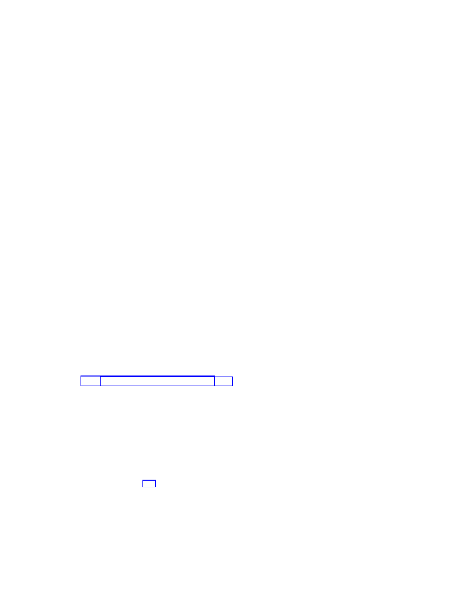
4 Reconstruction
42
The Heavy Top.
In this case, the coadjoint orbit equation is trivial and so the Lagrange–
Routh equations reduce to second order equations for Γ on S
2
. These equations are com-
puted to be as follows:
¨
Γ =
− ˙Γ
2
Γ + Γ
× Σ,
where
Σ = b ˙
Γ
− ν ˙Γ + I
−1
I( ˙
Γ
× Γ) + (ν − b)IΓ
×
( ˙
Γ
× Γ) + (ν − b)Γ
+ M glΓ
× χ
,
b = [( ˙
Γ
×Γ)·IΓ]/(Γ·IΓ), and ν = µ/(Γ·IΓ). Notice that one can write Σ = Σ
0
+µΣ
1
+µ
2
Σ
2
,
which represent the three terms in the Lagrange Routh equations that are independent of
µ, linear in µ, and quadratic in µ. In particular, the term linear in µ is the magnetic term:
Σ
1
= (Γ
· IΓ)
−1
− ˙Γ + I
−1
I( ˙
Γ
× Γ) × Γ + IΓ × ( ˙Γ × Γ)
.
This of course is the “curvature term” in the Lagrange–Routh equations. Notice that it is,
according to the general theory, linear in the “velocity” ˙
Γ. The remaining terms are the
Euler–Lagrange expression of the reduced Routhian with those quadratic in the velocity
being the differential of the amendment.
4
Reconstruction
4.1
First Reconstruction Equation
The Local Formula.
For a curve with known constant value of momentum, the evolution
of the group variable can be determined from the shape space trajectory. This reconstruc-
tion equation is usually written in a local trivialization S
× G of the bundle Q → Q/G
in the following way. Given a shape space trajectory x(t), the curve q(t) = (x(t), g(t)) has
momentum µ (i.e. J
L
(q(t), ˙q(t)) = µ) if and only if g(t) solves the differential equation
˙g = g
· [I
loc
(x)
−1
Ad
∗
g
µ
− A
loc
(x) ˙x]
(4.1)
Here, I
loc
is the local representative of the locked inertia tensor and A
loc
is the local rep-
resentative of the mechanical connection. This equation is one of the central objects in
the study of phases and locomotion and has an analogue for nonholonomic systems (see
Marsden, Montgomery and Ratiu [1990] and Bloch, Krishnaprasad, Marsden and Murray
[1996]).
The Intrinsic Equation.
We will now write this equation in an intrinsic way without
choosing a local trivialization.
Let x(t)
∈ S = Q/G be a given curve and let µ be a given value of the momentum map.
We want to find a curve q(t)
∈ Q that projects to x(t) and such that its tangent ˙q(t) lies in
the level set J
−1
L
(µ). We first choose any curve ˜
q(t)
∈ Q that projects to x(t). For example,
in a local trivialization, it could be the curve t
→ (x(t), e) or it could be the horizontal lift
of the base curve. Now we write q(t) = g(t)
· ˜q(t).
We shall now make use of the following formula for the derivatives of curves that was
given in equation (1.2):
˙q(t) =
Ad
g(t)
ξ(t)
Q
(q(t)) + g(t)
· ˙˜q(t),
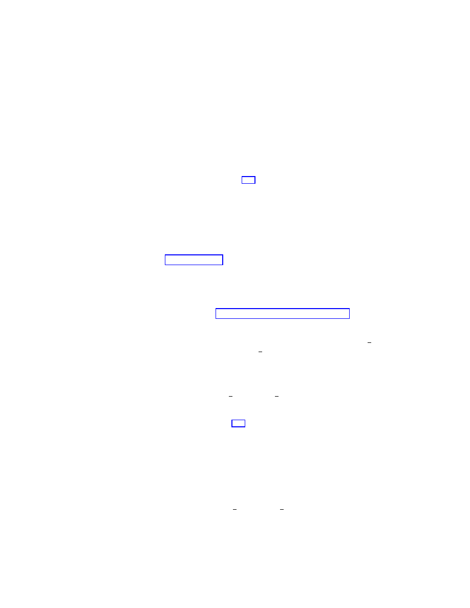
4.2 Second Reconstruction Equation
43
where ξ(t) = g(t)
−1
· ˙g(t). Applying the mechanical connection A to both sides, using the
identity A(v
q
) = I(q)
−1
· J
L
(v
q
), the fact that A(η
Q
(q)) = η, equivariance of the mechanical
connection, and assuming that ˙q(t)
∈ J
−1
L
(µ) gives
I(q)
−1
µ = Ad
g(t)
ξ(t) + Ad
g(t)
A( ˙˜
q(t)).
Solving this equation for ξ(t) gives
ξ(t) = Ad
g(t)
−1
I(q(t))
−1
µ
− A(˙˜q(t)).
Using equivariance of I leads to the first reconstruction equation:
g(t)
−1
˙g(t) = I(˜
q(t))
−1
Ad
∗
g(t)
µ
− A(˙˜q(t)).
(4.2)
Notice that this reproduces the local equation (4.1).
Example: The Rigid Body.
In this example, there is no second term in the preceding
equation since the bundle has a trivial base, so we choose ˜
q(t) to be the identity element.
Thus, this reconstruction process amounts to the following equation for the attitude matrix
A(t):
˙
A(t) = A(t)I
−1
A(t)
−1
π.
This is the method that Whittaker [1907] used to integrate for the attitude matrix.
4.2
Second Reconstruction Equation
In symplectic reconstruction, one needs only solve a differential equation on the subgroup
G
µ
instead of on G since the reduction bundle J
−1
(µ)
→ P
µ
= J
−1
(µ)/G
µ
is one that
quotients only by the subgroup G
µ
. See Marsden, Montgomery and Ratiu [1990] for details.
This suggests that one can do something similar from the Lagrangian point of view.
Second Reconstruction Equation.
Given a curve y(t)
∈ Q/G
µ
, we find a curve q(t)
∈
Q that projects to y(t). We now write q(t) = g(t)
· q(t) where g(t) ∈ G
µ
and require that
˙q(t)
∈ J
−1
L
(µ). Now we use the same formula for derivatives of curves as above and again
apply the mechanical connection for the G-action to derive the second reconstruction
equation
g(t)
−1
˙g(t) = I(q(t))
−1
µ
− A(˙q(t)).
(4.3)
Notice that we have Ad
∗
g(t)
µ = µ since g(t)
∈ G
µ
.
This second reconstruction equation (4.3) is now a differential equation on G
µ
, which
normally would be simpler to integrate than its counterpart equation on G. The reason we
are able to get an equation on a smaller group is because we are using more information,
namely that of y(t) as opposed to x(t).
The Abelian Case.
For generic µ
∈ g
∗
, the subgroup G
µ
is Abelian by a theorem of
Duflo and Vergne. In this Abelian case, the second reconstruction equation reduces to a
quadrature. One has, in fact,
g(t) = g(0) exp
t
0
I(q(s))
−1
µ
− A(˙q(s)
ds
.
(4.4)

4.3 Third Reconstruction Equation
44
Example: The Rigid Body.
In the case of the free rigid body, G = SO(3) and thus
if π
= 0, we have G
π
= S
1
, the rotations about the axis π. The above formula leads
to an expression for the attitude matrix that depends only on a quadrature as opposed
to nonlinear differential equations to be integrated. The curve y(t) is the body angular
momentum Π(t) and the momentum is the spatial angular momentum π. The curve q(t)
is the choice of a curve A(t) in SO(3) such that it rotates the vector Π(t) to the vector π.
For example, one can choose this rotation to be about the axis Π(t)
× π through the angle
given by the angle between the vectors Π(t) and π. Explicitly,
A(t) = exp
ϕ(t)
Π(t)
× π
Π(t) × π
!
,
(4.5)
where cos ϕ(t) = Π(t)
· π/π
2
.
The group element g(t) now is an angle α(t) that represents a rotation about the axis π
through the angle α(t). Then (4.4) becomes
α(t) = α(0) +
t
0
π
π
·
I(A(s))
−1
π
− A( ˙A(s))ˇ
ds
= α(0) +
t
0
π
π
·
A(s)I
−1
A(s)
−1
π
−
˙
A(s)A(s)
−1
ˇ
ds
.
Some remarks are in order concerning this formula. We have used the hat map and its
inverse, the check map, to identify
R
3
with so(3). In this case, the group elements in S
1
are identified with real numbers, namely, the angles of rotations about the axis π. Thus,
the product in the general formula (4.4) becomes a sum and the integral over the curve in
g
µ
becomes an ordinary integral. The integrand at first glance, is an element of g, but, of
course, it actually belongs to g
µ
. For the example of the rigid body, we make this explicitl
by taking the inner product with a unit vector along π.
4.3
Third Reconstruction Equation
The second reconstruction equation used the information on a curve y(t) in Q/G
µ
as opposed
to a curve x(t) in Q/G in order to enable one to integrate on the smaller, often Abelian, group
G
µ
. However, it still used the mechanical connection associated with the G-action. We can
derive yet a third reconstruction equation by using the mechanical connection associated
with the G
µ
-action.
The momentum map for the G
µ
-action on T Q is given by J
G
µ
L
= ι
∗
µ
◦J
L
where ι
µ
: g
µ
→ g
is the inclusion and where ι
∗
µ
: g
∗
→ g
∗
µ
is its dual (the projection, or restriction map). We
can also define the locked inertia tensor and mechanical connection for the G
µ
-action, in
the same way as was done for the G-action. We denote these by
I
G
µ
(q) = ι
∗
µ
◦ I(q) ◦ ι
µ
: g
µ
→ g
∗
µ
and
A
G
µ
: T Q
→ g
µ
.
In the third reconstruction equation we organize the logic a little differently and in effect,
take dynamics into account. Namely, we assume we have a curve q(t)
∈ J
−1
L
(µ), for example,
a solution of the Euler–Lagrange equations with initial conditions in J
−1
L
(µ). We now let
y(t)
∈ Q/G
µ
be the projection of q(t). We also let µ = ι
∗
µ
µ = µ
|g
µ
. We first choose any
curve q(t)
∈ Q that projects to y(t). For example, as before, in a local trivialization, it could
be the curve t
→ (y(t), e) or it could be the horizontal lift of y(t) relative to the connection
A
G
µ
. Now we write q(t) = g(t)
· q(t), where g(t) ∈ G
µ
.
As before, we use the following formula for the derivatives of curves:
˙q(t) =
Ad
g(t)
ξ(t)
Q
(q(t)) + g(t)
· ˙q(t),
4.4 The Vertical Killing Metric
45
where ξ(t) = g(t)
−1
· ˙g(t) ∈ g
µ
. Applying the mechanical connection A
G
µ
to both sides,
using the identity A
G
µ
(v
q
) = I
G
µ
(q)
−1
·J
G
µ
L
(v
q
), the fact that A
G
µ
(η
Q
(q)) = η, equivariance
of the mechanical connection gives
I
G
µ
(q)
−1
µ = Ad
g(t)
ξ(t) + Ad
g(t)
A
G
µ
( ˙q(t)).
Solving this equation for ξ(t) gives ξ(t) = Ad
g(t)
−1
I
G
µ
(q(t))
−1
µ
− A
G
µ
( ˙q(t)). Using equiv-
ariance of I
G
µ
leads to g(t)
−1
˙g(t) = I
G
µ
(q(t))
−1
Ad
∗
g(t)
µ
− A
G
µ
( ˙q(t)), where in the last
equation, Ad
∗
g(t)
is the coadjoint action for G
µ
. One checks that Ad
∗
g(t)
µ = µ, using the
fact that g(t)
∈ G
µ
, so this equation becomes
g(t)
−1
˙g(t) = I
G
µ
(q(t))
−1
µ
− A
G
µ
( ˙q(t)).
(4.6)
The same remarks as before apply concerning the generic Abelian nature of G
µ
applied to
this equation. In particular, when G
µ
is Abelian, we have the formula
g(t) = g(0) exp
t
0
I
G
µ
(q(s))
−1
µ
− A
G
µ
( ˙q(s)
ds
(4.7)
Example: The Rigid Body.
Here we start with a solution of the Euler–Lagrange equa-
tions A(t) and we let π be the spatial angular momentum and Π(t) be the body angular
momentum. We choose the curve A(t) using formula (4.5). We now want to calculate the
angle α(t) of rotation around the axis π such that A(t) = R
α,π
A(t), where R
α,π
denotes
the rotation about the axis π through the angle α. In this case, we get
α(t) = α(0) +
t
0
I
G
µ
(A(s))
−1
µ
− A
G
µ
( ˙
A(s)
ds
(4.8)
Now we identify g
µ
with
R by the isomorphism a → aπ/π. Then, for B ∈ SO(3)
I
G
µ
(B) =
π
· (BIB
−1
)π
π
2
Taking B = A(s), and using the fact that A(s) maps Π(s) to π, we get
I
G
µ
(A(s))
−1
=
π
2
π
· (A(s)IA(s)
−1
)π
=
π
2
Π(s)
· IΠ(s)
The element µ is represented, according to our identifications, by the number
π, so
I
G
µ
(A(s))
−1
µ =
π
3
Π(s)
· IΠ(s)
Thus, (4.8) becomes
α(t) = α(0) +
t
0
π
3
Π(s)
· IΠ(s)
− A
G
µ
˙
A(s)
ds
.
(4.9)
This formula agrees with that found in Marsden, Montgomery and Ratiu [1990],
§5.1.2.
4.4
The Vertical Killing Metric
For some calculations as well as a deeper insight into geometric phases studied in the next
section, it is convenient to introduce a modified metric.

4.4 The Vertical Killing Metric
46
Definition of the Vertical Killing Metric.
First, we assume that the Lie algebra g
has an inner product which we shall denote
· , ·
◦
, with the property that Ad
g
: g
→ g is
orthogonal for every g. For example, if G is compact, the negative of the Killing form is such
a metric. For SO(3), we shall use the standard dot product as this metric. For convenience,
we shall refer to the inner product
· , ·
◦
as the Killing metric.
Now we use the Killing metric on g to define a new metric on Q by using the same
horizontal and vertical decomposition given by the mechanical connection of the original
(kinetic energy) metric. On the horizontal space we use the given inner product while on
the vertical space, we take the inner product of two vertical vectors, say ξ
Q
(q) and η
Q
(q)
to be
ξ , η
◦
. Finally, in the new metric we declare the horizontal and vertical spaces to
be orthogonal. These properties define the new metric, which we shall call the vertical
Killing metric.
The metric
· , ·
◦
is easily checked to be G-invariant, so we can repeat the previous
constructions for it. In particular, since the horizontal spaces are unchanged, the mechanical
connection on the bundle Q
→ Q/G is identical to what it was before. However, for our
purposes, we are more interested in the connection on the bundle Q
→ Q/G
µ
; here the
connections need not be the same.
The Mechanical Connection in terms of the Vertical Killing Metric.
We now
compute the momentum map J
◦
and the locked inertia tensor I
◦
for the metric
· , ·
◦
associated with the G-action on Q. Notice that by construction, the mechanical connection
associated with this metric is identical to that for the kinetic energy metric.
First of all, the locked inertia tensor I
◦
(q) : g
→ g
∗
is given by
I
◦
(q)ξ, η
= ξ
Q
(q), η
Q
(q)
◦
=
ξ, η
◦
.
In other words, the locked inertia tensor for the vertical Killing metric is simply the map
associated with the Killing metric on the Lie algebra.
Next, we compute the momentum map J
◦
: T Q
→ g
∗
associated with the vertical Killing
metric. For η
∈ g
µ
, we have, by definition,
J
◦
(v
q
), η
= v
q
, η
Q
(q)
◦
=
Hor(v
q
) + V er(v
q
), η
Q
(q)
◦
=
A(v
q
), η
◦
,
where A is the mechanical connection for the G-action.
Notice that these quantities are related by
A(v
q
) = I
◦
(q)
−1
J
◦
(v
q
).
(4.10)
It is interesting to compare this with the similar formula (1.1) for A using the kinetic energy
metric.
The G
µ
-connection in the Vertical Killing Metric.
We now compute the momentum
map J
G
µ
◦
, the locked inertia tensor I
G
µ
◦
and the mechanical connection A
G
µ
◦
for the metric
· , ·
◦
and the G
µ
-action on Q.
First of all, the locked inertia tensor I
G
µ
◦
(q) : g
µ
→ g
∗
µ
is given by
I
G
µ
◦
(q)ξ, η
=
ξ
Q
(q), η
Q
(q)
◦
=
ξ, η
◦
.
6
This metric has been used by a variety ofauthors, such as Montgomery [1990, 1991a]. Related modifica-
tions ofthe kinetic energy metric are used by Bloch, Leonard and Marsden [1998, 1999] for the stabilization
ofrelative equilibria ofmechanical control systems. and shall denote it
· , ·
◦
.
4.5 Fourth Reconstruction Equation
47
Next, we compute J
G
µ
◦
: T Q
→ g
∗
µ
; for η
∈ g
µ
, we have
J
G
µ
◦
(v
q
), η
=
v
q
, η
Q
(q)
◦
=
Hor(v
q
) + V er(v
q
), η
Q
(q)
◦
=
A(v
q
), η
◦
=
pr
µ
A(v
q
), η
◦
,
where A is the mechanical connection for the G-action (for either the original or the modified
metric) and where pr
µ
: g
→ g
µ
is the orthogonal projection with respect to the metric
· , ·
◦
onto g
µ
.
As before, these quantities are related by A
G
µ
◦
(v
q
) = I
G
µ
◦
(q)
−1
J
G
µ
◦
(v
q
), and so from the
preceding two relations, it follows that A
G
µ
◦
(v
q
) = pr
µ
A(v
q
).
The Connection on the Bundle ρ
µ
.
We just computed the mechanical connection on
the bundle π
Q,G
µ
: Q
→ Q/G
µ
associated with the vertical Killing metric. There is a similar
formula for that associated with the kinetic energy metric. In particular, it follows that in
general, these two connections are different. This difference is important in the next section
on geometric phases.
Despite this difference, it is interesting to note that each of them induces the same
Ehresmann connection on the bundle ρ
µ
: Q/G
µ
→ Q/G. Thus, in splitting the Lagrange–
Routh equations into horizontal and vertical parts, there is no difference between using the
kinetic energy metric and the vertical Killing metric.
4.5
Fourth Reconstruction Equation
There is yet a fourth reconstruction equation that is based on a different connection. The
new connection will be that associated with the vertical Killing metric.
As before, we first choose any curve q(t)
∈ Q that projects to y(t). For example, in a
local trivialization, it could be the curve t
→ (y(t), e) or it could be the horizontal lift of y(t)
relative to the connection A
G
µ
◦
. Now we write q(t) = g(t)
· q(t), where g(t) ∈ G
µ
. Again, we
use the following formula for the derivatives of curves:
˙q(t) =
Ad
g(t)
ξ(t)
Q
(q(t)) + g(t)
· ˙q(t),
(4.11)
where ξ(t) = g(t)
−1
· ˙g(t) ∈ g
µ
.
Now we assume that ˙q(t)
∈ J
−1
L
(µ) and apply the connection A
G
µ
◦
to both sides. The
left hand side of (4.11) then becomes
A
G
µ
◦
( ˙q(t)) = pr
µ
A( ˙
q(t)) = pr
µ
I(q(t))
−1
J
L
( ˙q(t)) = pr
µ
I(q(t))
−1
µ.
The right hand side of (4.11) becomes Ad
g(t)
ξ(t) + Ad
g(t)
A
G
µ
◦
( ˙q(t)). Thus, we have proved
that
pr
µ
I(q(t))
−1
µ = Ad
g(t)
ξ(t) + A
G
µ
◦
( ˙q(t))
.
Solving this equation for ξ(t) and using the fact that Ad
g(t)
is orthogonal in the Killing
inner product on g gives
ξ(t) = Ad
g(t)
−1
pr
µ
I(q(t))
−1
µ
− A
G
µ
◦
( ˙q(t))
= pr
µ
Ad
g(t)
−1
I(q(t))
−1
µ
− A
G
µ
◦
( ˙q(t)).
4.6 Geometric Phases
48
Using equivariance of I leads to the fourth reconstruction equation for q(t) = g(t)
·q(t) ∈
J
−1
L
(µ) given y(t)
∈ Q/G
µ
:
g(t)
−1
˙g(t) = pr
µ
I(q(t))
−1
µ
− A
G
µ
◦
( ˙q(t)),
(4.12)
where, recall, q(t) is any curve in Q such that [q(t)]
G
µ
= y(t).
When G
µ
is Abelian, we have, as with the other reconstruction equations,
g(t) = g(0) exp
t
0
pr
µ
I(q(s))
−1
µ
− A
G
µ
◦
( ˙q(s))
ds
(4.13)
4.6
Geometric Phases
Once one has formulas for the reconstruction equation, one gets formulas for geometric
phases as special cases. Recall that geometric phases are important in a wide variety of
phenomena such as control and locomotion generation (see Marsden and Ostrowski [1998]
and Marsden [1999] for accounts and further literature).
The way one proceeds in each case is similar. We consider a closed curve y(t) in Q/G
µ
,
with, say, 0
≤ t ≤ T and lift it to a curve q(t) according to one of the reconstruction equations
in the preceding sections. Then we can write the final point q(T ) as q(T ) = g
tot
q(0), which
defines the total phase, g
tot
. The group element g
tot
will be in G or in G
µ
according to
which reconstruction formula is used.
For example, suppose that one uses equation (4.12) with q(t) chosen to be the horizontal
lift of y(t) with respect to the connection A
G
µ
◦
with initial conditions q
0
covering y(0). Then
q(T ) = g
geo
q
0
, where g
geo
is the holonomy of the base curve y(t). This group element is
called the geometric phase. Then we get q(T ) = g
dyn
g
geo
q(0) where g
dyn
= g(T ), and g(t)
is the solution of g(t)
−1
˙g(t) = I(q(t))
−1
µ in the group G
µ
with g(0) the identity. The group
element g
dyn
is often called the dynamic phase. Thus, we have g
tot
= g
dyn
g
geo
. Of course
in case G
µ
is Abelian, this group multiplication is given by addition and the dynamic phase
is given by the explicit integral
g
dyn
=
T
0
pr
µ
I(q(s))
−1
µ
ds.
Example: The Rigid Body
In the case of the rigid body, the holonomy is simply given
by the symplectic area on the coadjoint orbit S
2
since the curvature, as we have seen, is,
in this case, the symplectic form and since the holonomy is given by the integral of the
curvature over a surface bounding the given curve (see, e.g., Kobayashi and Nomizu [1963]
or Marsden, Montgomery and Ratiu [1990] for this classical formula for holonomy).
We now compute the dynamic phase. Write the horizontal lift as A so that we have, as
before, A(t)Π(t) = π, A(t)Π(t) = π and A(t) = R
α,π
(t)A(t).
Now I(A(t)) = A(t)IA(t)
−1
. Therefore,
I(
A(t))
−1
π = A(t)I
−1
A
−1
(t)π = A(t)I
−1
Π(t) = A(t)Ω(t).
But then
pr
µ
I(
q(s))
−1
µ
= pr
π
I(
A(s))
−1
π
= I(A(s))
−1
π
·
π
π
= A(s)Ω(s)
·
π
π
= Ω
·
A(s)
−1
π
π
=
Ω
· Π
π
=
2E
π
,
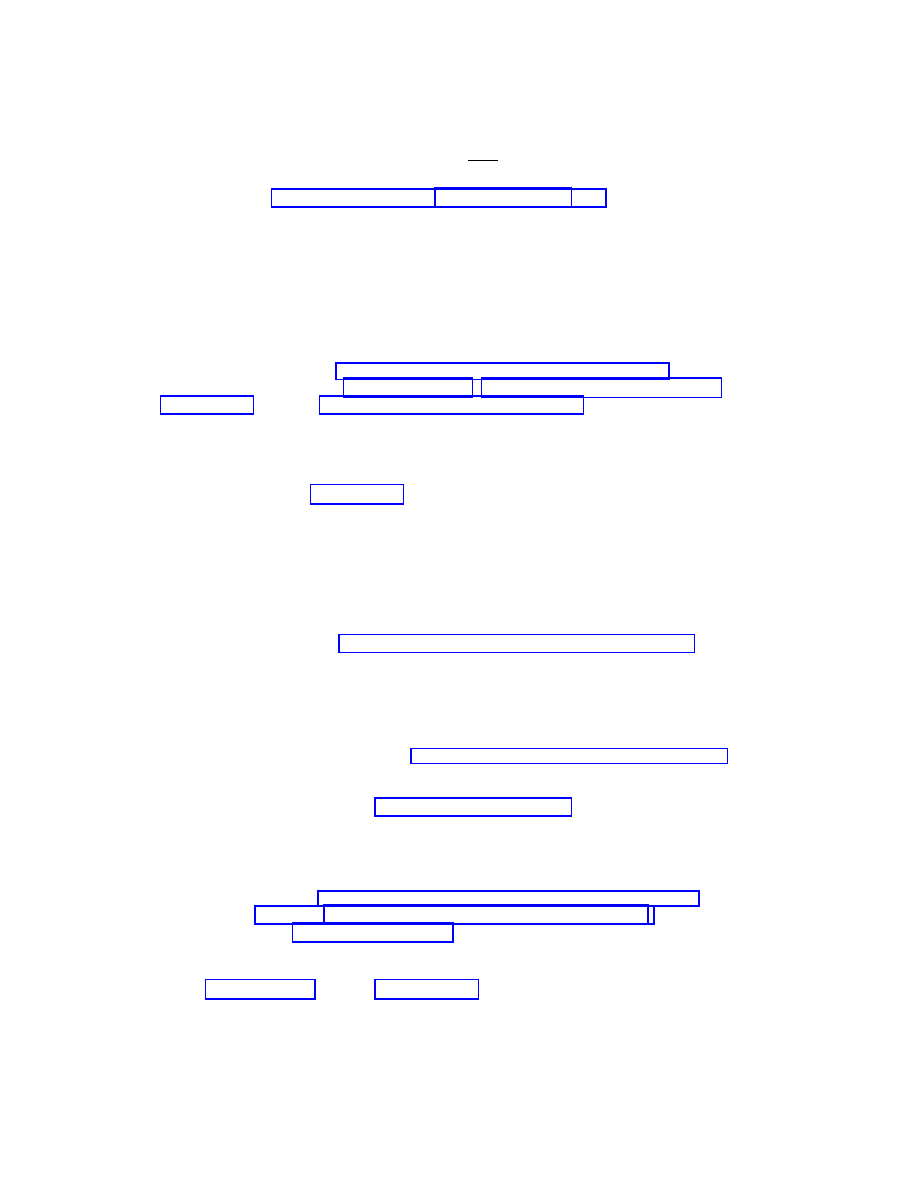
5 Future Directions and Open Questions
49
where E is the energy of the trajectory. Thus, the dynamic phase is given by
g
dyn
=
2ET
π
which is the rigid body phase formula of Montgomery [1991b] and Marsden, Montgomery
and Ratiu [1990].
5
Future Directions and Open Questions
The Hamiltonian Bundle Picture.
As we have described earlier, on the Lagrangian
side, we choose a connection on the bundle π
Q,G
: Q
→ Q/G and realize T Q/G as the
Whitney sum bundle T (Q/G)
⊕ ˜g over Q/G. Correspondingly, on the Hamiltonian side we
realize T
∗
Q/G as the Whitney sum bundle T
∗
(Q/G)
⊕ ˜g
∗
over Q/G. The reduced Poisson
structure on this space, as we have mentioned already, has been investigated by Montgomery,
Marsden and Ratiu [1984], Montgomery [1986], Cendra, Marsden and Ratiu [2000a], and
Zaalani [1999]. See also Guillemin, Lerman and Sternberg [1996] and references therein.
The results of the present paper on Routh reduction show that on the Lagrangian side,
the reduced space J
−1
L
(µ)/G
µ
is T (Q/G)
×
Q/G
Q/G
µ
. This is consistent (by taking the dual
of our isomorphism of bundles) with the fact that the symplectic leaves of (T
∗
Q)/G can be
identified with T
∗
(Q/G)
×
Q/G
µ
. The symplectic structure on these leaves has been
investigated by ?] and Zaalani [1999]. It would be interesting to see if the techniques of the
present paper shed any further light on these constructions.
In the way we have set things up, we conjecture that the symplectic structure on
T
∗
(Q/G)
×
Q/G
Q/G
µ
is the canonical cotangent symplectic form on T
∗
(Q/G) plus β
µ
(that
is, the canonical cotangent symplectic form plus Curv
(x,µ)
A
, the (x, µ)-component of the
curvature of the mechanical connection, x
∈ Q/G, pulled up from Q/G to T
∗
(Q/G)) plus
the coadjoint orbit symplectic form on the fibers.
It would also be of interest to see to what extend one can derive the symplectic (and
Poisson) structures directly from the variational principle as boundary terms, as in Marsden,
Patrick and Shkoller [1998].
Singular Reduction and Bifurcation.
We mentioned the importance of singular reduc-
tion in the introduction. However, almost all of the theory of singular reduction is confined
to the general symplectic category, with little attention paid to the tangent and cotangent
bundle structure. However, explicit examples, as simple as the spherical pendulum (see Ler-
man, Montgomery and Sjamaar [1993]) show that this cotangent bundle structure together
with a “stitching construction” is important.
As was mentioned already in Marsden and Scheurle [1993a] in connection with the dou-
ble spherical pendulum, it would be interesting to develop the general theory of singular
Lagrangian reduction using, amongst other tools, the techniques of blow up. In addition,
this should be dual to a similar effort for the general theory of symplectic reduction of cotan-
gent bundles. We believe that the general bundle structures in this paper will be useful for
this endeavor. The links with bifurcation with symmetry are very interesting; see Golubit-
sky and Schaeffer [1985], Golubitsky, Marsden, Stewart and Dellnitz [1995], Golubitsky and
Stewart [1987], and Ortega and Ratiu [1997], for instance.
Groupoids.
There is an approach to Lagrangian reduction using groupoids and algebroids
due to Weinstein [1996] (see also Martinez [1999]). It would of course be of interest to make
additional links between these approaches and the present ones.
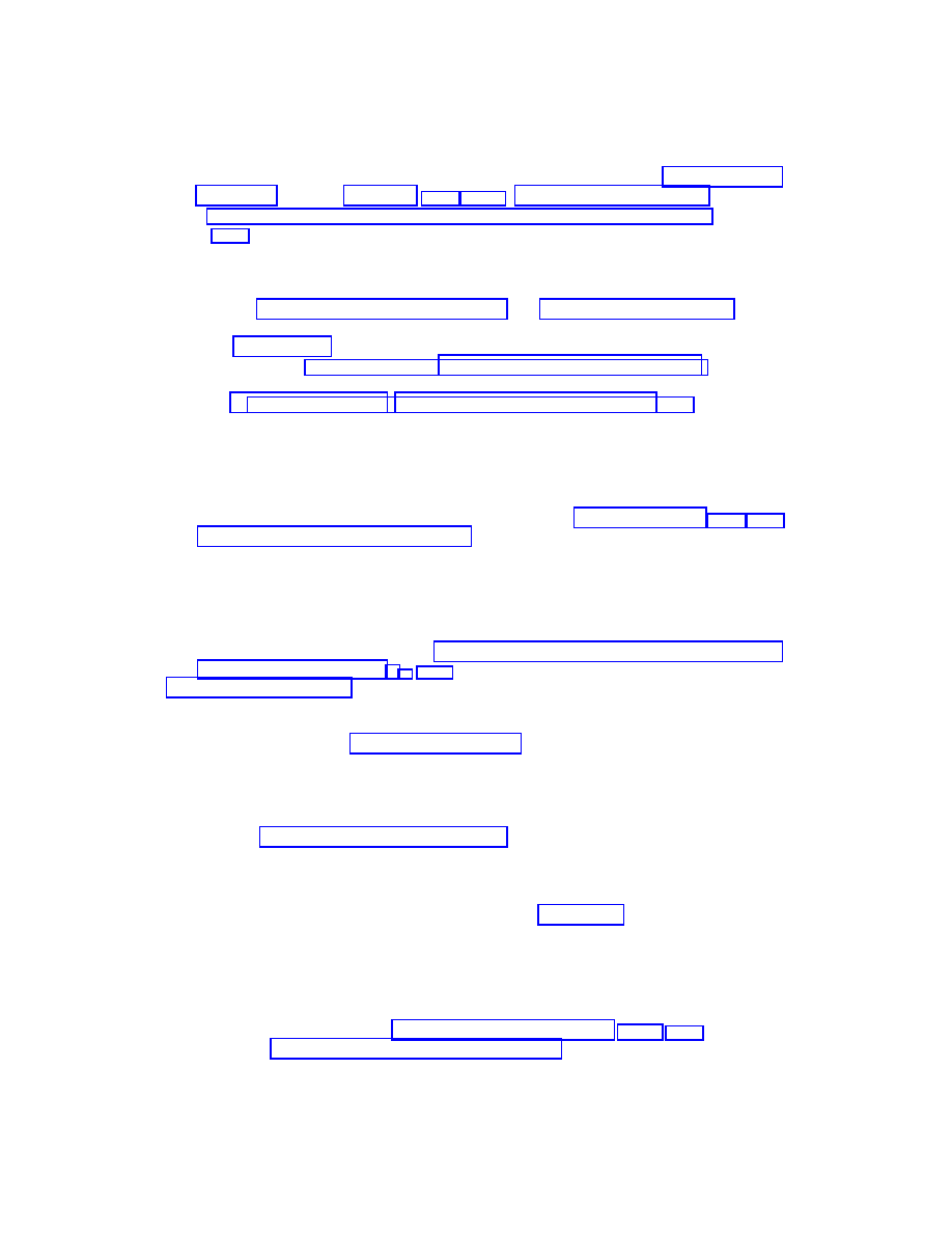
5 Future Directions and Open Questions
50
Quantum Systems.
The bundle picture in mechanics is clearly important in understand-
ing quantum mechanical systems, and the quantum–classical relationship. For example, the
mechanical connection has already proved useful in understanding the relation between vi-
bratory and rotational modes of molecules. This effort really started with Guichardet [1984]
and Iwai [1987c]. See also Iwai [1982, 1985, 1987a]. Littlejohn and Reinch [1997] (and other
recent references as well) have carried on this work in a very interesting way. Landsman
[1995, 1998] also uses reduction theory in an interesting way.
Multisymplectic Geometry and Variational Integrators.
There have been signifi-
cant developments in multisymplectic geometry that have led to interesting integration algo-
rithms, as in Marsden, Patrick and Shkoller [1998] and Marsden and Shkoller [1999]. There
is also all the work on reduction for discrete mechanics which also takes a variational view,
following Veselov [1988]. These variational integrators have been important in numerical
integration of mechanical systems, as in Kane, Marsden, Ortiz and West [2000], Wendlandt
and Marsden [1997] and references therein. Discrete analogues of reduction theory have
begun in Ge and Marsden [1988], Marsden, Pekarsky and Shkoller [1999], and Bobenko and
Suris [1998]. We expect that one can generalize this theory from the Euler–Poincar´
e and
semidirect product context to the context of general configuration spaces using the ideas of
Lagrange–Routh reduction in the present work.
Geometric Phases.
In this paper we have begun the development of the theory of geo-
metric phases in the Lagrangian context building on work of Montgomery [1985, 1988, 1993]
and Marsden, Montgomery and Ratiu [1990]. In fact, the Lagrangian setting also provides
a natural setting for averaging which is one of the basic ingredients in geometric phases.
We expect that our approach will be useful in a variety of problems involving control and
locomotion.
Nonholonomic Mechanics.
Lagrangian reduction has had a significant impact on the
theory of nonholonomic systems, as in Bloch, Krishnaprasad, Marsden and Murray [1996]
and Koon and Marsden [1997a,b,c, 1998]. The almost symplectic analogue was given in
Bates and Sniatycki [1993]. These references also develop Lagrangian reduction methods
in the context of nonholonomic mechanics with symmetry (such as systems with rolling
constraints). These methods have also been quite useful in many control problems and in
robotics; see, for example, Bloch and Crouch [1999]. One of the main ingredients in these
applications is the fact that one no longer gets conservation laws, but rather one replaces the
momentum map constraint with a momentum equation. It would be of considerable interest
to extend the reduction ideas of the present paper to that context. A Lagrange–d’Alembert–
Poincar´e reduction theory, the nonholonomic version of Lagrange–Poincar´
e reduction, is
considered in Cendra, Marsden and Ratiu [2000b].
Stability and Block Diagonalization.
Further connections and development of stability
and bifurcation theory on the Lagrangian side (also in the singular case) would also be of
interest. Already a start on this program is done by Lewis [1992]. Especially interesting
would be to reformulate Lagrangian block diagonalization in the current framework. We
conjecture that the structure of the Lagrange–Routh equations given in the present paper
is in a form for which block diagonalization is automatically and naturally achieved.
Fluid Theories.
The techiques of Lagrangian reduction have been very useful in the study
of interesting fluid theories, as in Holm, Marsden and Ratiu [1986, 1998b, 1999] and plasma
theories, as in Cendra, Holm, Hoyle and Marsden [1998], including interesting analytical
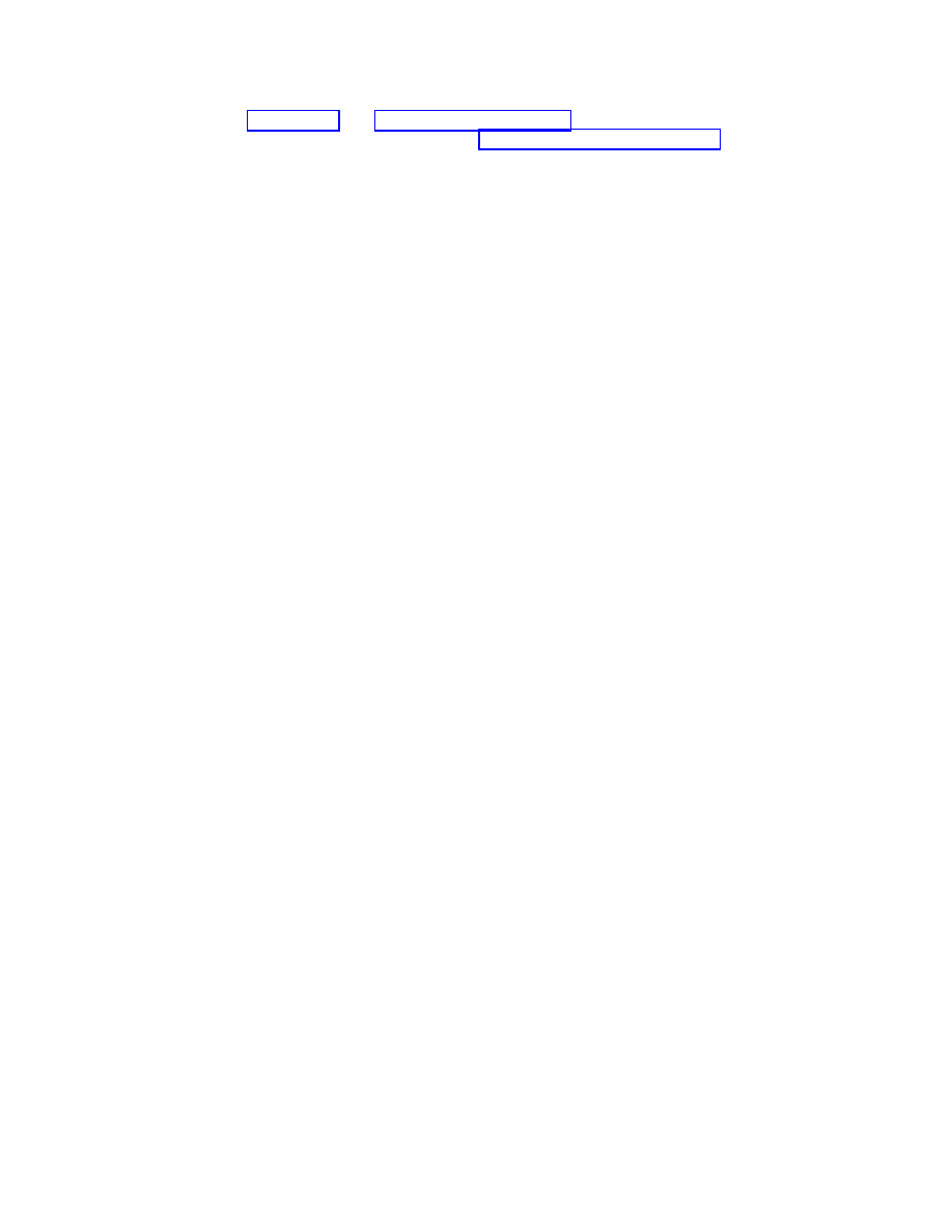
REFERENCES
51
tools (as in Cantor [1975] and Nirenberg and Walker [1973]). Amongst these, the averaged
Euler equations are especially interesting; see Marsden, Ratiu and Shkoller [1999].
Routh by Stages
In the text we discussed the current state of affairs in the theory of
reduction by stages, both Lagrangian and Hamiltonian. The Lagrangian counterpart of
symplectic reduction is of course what we have developed here, namely Lagrange–Routh
reduction. Naturally then, the development of this theory for reduction by stages for group
extensions would be very interesting.
Acknowledgement:
We thank our many collaborators and students for their help, direct
or indirect, with this paper. In particular, we would like to single out Anthony Blaom, An-
thony Bloch, Sameer Jalnapurkar, Hans-Peter Kruse, Melvin Leok, Naomi Leonard, Sergey
Pekarsky, Matt Perlmutter, Steve Shkoller, Alan Weinstein, and Matt West.
References
Abarbanel, H. D. I., D. D. Holm, J. E. Marsden and T. S. Ratiu [1986], Nonlinear stability
analysis of stratified fluid equilibria, Phil. Trans. Roy. Soc. London A, 318, 349–409; (See
also Richardson number criterion for the nonlinear stability of three-dimensional stratified
flow, Phys. Rev. Lett. 52 (1984), 2552–2555).
Abraham, R. and J. E. Marsden [1978], Foundations of Mechanics, Addison-Wesley, Second
edition.
Abraham, R., J. E. Marsden and T. S. Ratiu [1988], Manifolds, Tensor Analysis and Ap-
plications, Applied Mathematical Sciences, 75, Springer-Verlag, Second edition.
Alber, M. S., G. G. Luther, J. E. Marsden and J. M. Robbins [1998], Geometric phases,
reduction and Lie-Poisson structure for the resonant three-wave interaction, Physica D,
123, 271–290.
Arms, J. M., R. H. Cushman and M. Gotay [1991], A universal reduction procedure for
Hamiltonian group actions, in The Geometry of Hamiltonian systems, T. Ratiu, ed.,
MSRI Series, 22, 33–52, Springer-Verlag.
Arms, J. M., J. E. Marsden and V. Moncrief [1981], Symmetry and bifurcations of momen-
tum mappings, Comm. Math. Phys., 78, 455–478.
Arms, J. M., J. E. Marsden and V. Moncrief [1982], The structure of the space solutions
of Einstein’s equations: II Several Killings fields and the Einstein–Yang–Mills equations,
Ann. of Phys., 144, 81–106.
Arnold, V. I. [1966a], Sur la g´
eom´etrie differentielle des groupes de Lie de dimenson infinie
et ses applications `
a l’hydrodynamique des fluidsparfaits, Ann. Inst. Fourier, Grenoble,
16, 319–361.
Arnold, V. I. [1966b], On an a priori estimate in the theory of hydrodynamical stability,
Izv. Vyssh. Uchebn. Zaved. Mat. Nauk , 54, 3–5; English Translation: Amer. Math. Soc.
Transl. 79 (1969), 267–269.
Arnold, V. I. [1966c], Sur un principe variationnel pour les d´
ecoulements stationnaires des
liquides parfaits et ses applications aux problemes de stabilit´
e non lin´eaires, J. M´
ecanique,
5, 29–43.

REFERENCES
52
Arnold, V. I., V. V. Kozlov and A. I. Neishtadt [1988],Mathematical aspects of Classical and
Celestial Mechanics; Dynamical Systems III , V. I. Arnold, ed., Springer-Verlag.
Arnold, V. I. [1989], Mathematical Methods of Classical Mechanics, Graduate Texts in
Math., 60, Springer-Verlag, Second edition.
Bates, L. and E. Lerman [1997], Proper group actions and symplectic stratified spaces,
Pacific J. Math., 181, 201–229.
Bates, L. and J. Sniatycki [1993], Nonholonomic reduction, Reports on Math. Phys., 32,
99–115.
Bloch, A. M. and P.
E.
Crouch [1999], Optimal control, optimization, and analytical
mechanics, in Mathematical control theory, 268–321, A K Peters, New York.
Bloch, A. M., P. S. Krishnaprasad, J. E. Marsden and R. Murray [1996], Nonholonomic
mechanical systems with symmetry, Arch. Rational Mech. Anal., 136, 21–99.
Bloch, A. M., P. S. Krishnaprasad, J. E. Marsden and T. S. Ratiu [1996], The Euler–Poincar´
e
equations and double bracket dissipation, Comm. Math. Phys., 175, 1–42.
Bloch, A. M., N. Leonard and J. E. Marsden [1998], Matching and Stabilization by the
Method of Controlled Lagrangians, in Proc. CDC , 37, 1446–1451.
Bloch, A. M., N. Leonard and J. E. Marsden [1999], Controlled Lagrangians and the Sta-
bilization of Mechanical Systems I: The First Matching Theorem, IEEE Trans. Automat.
Control ; (to appear).
Bobenko, A. I., A. G. Reyman and M. A. Semenov-Tian-Shansky [1989], The Kowalewski
Top 99 years later: A Lax pair, generalizations and explicit solutions, Comm. Math.
Phys., 122, 321–354.
Bobenko, A. I. and Y. B. Suris [1998], Discrete time Lagrangian mechanics on Lie groups,
with an application to the Lagrange top, Preprint.
Bretherton, F. P. [1970], A note on Hamilton’s principle for perfect fluids, J. Fluid Mech.,
44, 19–31.
Cantor, M. [1975], Spaces of functions with asymptotic conditions on
R
n
, Indiana. Univ.
Math. J., 24, 897–902.
Cendra, H., D. D. Holm, M. J. W. Hoyle and J. E. Marsden [1998], The Maxwell–Vlasov
equations in Euler–Poincar´
e form, J. Math. Phys., 39, 3138–3157.
Cendra, H., D. D. Holm, J. E. Marsden and T. S. Ratiu [1998], Lagrangian Reduction,
the Euler–Poincar´
e Equations and Semidirect Products, Amer. Math. Soc. Transl., 186,
1–25.
Cendra, H., A. Ibort and J. E. Marsden [1987], Variational principal fiber bundles: a geo-
metric theory of Clebsch potentials and Lin constraints, J. Geom. Phys., 4, 183–206.
Cendra, H. and J. E. Marsden [1987], Lin constraints, Clebsch potentials and variational
principles, Physica D, 27, 63–89.
Cendra, H., J. E. Marsden and T. S. Ratiu [2000a], Lagrangian reduction by stages, Mem.
Amer. Math. Soc.; (to appear).

REFERENCES
53
Cendra, H., J. E. Marsden and T. S. Ratiu [2000b], Geometric Mechanics, Lagrangian
Reduction and Nonholonomic Systems, in Mathematics Unlimited , Springer-Verlag, New
York; (to appear).
Chetayev, N. G. [1941], On the equations of Poincar´
e, J. Appl. Math. Mech., 5, 253–262.
Chetayev, N. G. [1961], The Stability of Motion, Pergamon.
Chetayev, N. G. [1989], Theoretical Mechanics, Springer-Verlag.
Cushman, R. and L. Bates [1997], Global Aspects of Classical Integrable Systems, Birkh¨
auser,
Boston.
Ebin, D. G. and J. E. Marsden [1970], Groups of diffeomorphisms and the motion of an
incompressible fluid, Ann. of Math., 92, 102–163.
Ge, Z. and J. E. Marsden [1988], Lie–Poisson integrators and Lie–Poisson Hamilton–Jacobi
theory, Phys. Lett. A, 133, 134–139.
Golubitsky, M., J. E. Marsden, I. Stewart and M. Dellnitz [1995], The constrained Liapunov
Schmidt procedure and periodic orbits, Fields Inst. Commun., 4, 81–127.
Golubitsky, M. and D. Schaeffer [1985], Singularities and Groups in Bifurcation Theory.
Vol. 1, Applied Mathematical Sciences, 69, Springer-Verlag.
Golubitsky, M. and I. Stewart [1987], Generic bifurcation of Hamiltonian systems with
symmetry, Physica D, 24, 391–405.
Golubitsky, M., I. Stewart and D. Schaeffer [1988], Singularities and Groups in Bifurcation
Theory. Vol. 2, Applied Mathematical Sciences, 69, Springer-Verlag.
Guichardet, A. [1984], On rotation and vibration motions of molecules, Ann. Inst. H.
Poincar´
e, 40, 329–342.
Guillemin, V., E. Lerman and S. Sternberg [1996], Symplectic Fibrations and Multiplicity
Diagrams, Cambridge University Press.
Guillemin, V. and E. Prato [1990], Heckman, Kostant and Steinberg formulas for symplectic
manifolds, Adv. in Math., 82, 160–179.
Guillemin, V. and S. Sternberg [1978], On the equations of motions of a classic particle in
a Yang–Mills field and the principle of general covariance, Hadronic J., 1, 1–32.
Guillemin, V. and S. Sternberg [1980], The moment map and collective motion, Ann. of
Phys., 1278, 220–253.
Guillemin, V. and S. Sternberg [1982], Convexity properties of the moment map, Invent.
Math., 67, 491–513; also 77, pp. 533–546.
Guillemin, V. and S. Sternberg [1984], Symplectic Techniques in Physics, Cambridge Uni-
versity Press.
Hamel, G. [1904], Die Lagrange–Eulerschen Gleichungen der Mechanik, Z. f¨
ur Mathematik
u. Physik , 50, 1–57.
Hamel, G. [1949], Theoretische Mechanik, Springer-Verlag.
Holm, D. D. and B. A. Kuperschmidt [1983], Poisson brackets and clebsch representations
for magnetohydrodynamics, multifluid plasmas and elasticity, Physica D, 6, 347–363.

REFERENCES
54
Holm, D. D. and B. A. Kupershmidt [1983], Poisson structures and superconductors, Lett.
A, 93, 177–181.
Holmes, P. J. and J. E. Marsden [1983], Horseshoes and Arnold diffusion for Hamiltonian
systems on Lie groups, Indiana Univ. Math. J., 32, 273–310.
Holm, D. D., J. E. Marsden and T. S. Ratiu [1986], The Hamiltonian structure of con-
tinuum mechanics in material, spatial and convective representations, in S´
eminaire de
Math´
ematiques sup´
erieurs, 100, 11–122, Les Presses de L’Univ. de Montr´eal.
Holm, D. D., J. E. Marsden and T. S. Ratiu [1998a], The Euler–Poincar´
e equations and
semidirect products with applications to continuum theories, Adv. in Math., 137, 1–8.
Holm, D. D., J. E. Marsden and T. S. Ratiu [1998b], Euler–Poincar´
e models of ideal fluids
with nonlinear dispersion, Phys. Rev. Lett., 349, 4173–4177.
Holm, D. D., J. E. Marsden and T. Ratiu [1999], The Euler–Poincar´
e equations in geo-
physical fluid dynamics, in Proceedings of the Isaac Newton Institute Programme on the
Mathematics of Atmospheric and Ocean Dynamics, Cambridge University Press;
(to
appear).
Holm, D. D., J. E. Marsden, T. S. Ratiu and A. Weinstein [1985], Nonlinear stability of
fluid and plasma equilibria, Phys. Rep., 123, 1–6.
Iwai, T. [1982], The symmetry group of the harmonic oscillator and its reduction, J. Math.
Phys., 23, 1088–1092.
Iwai, T. [1985], On reduction of two degrees of freedom Hamiltonian systems by an S
1
action
and SO
0
(1, 2) as a dynamical group, J. Math. Phys., 26, 885–893.
Iwai, T. [1987a], A gauge theory for the quantum planar three-body system, J. Math. Phys.,
28, 1315–1326.
Iwai, T. [1987b], A geometric setting for internal motions of the quantum three-body system,
J. Math. Phys., 28, 1315–1326.
Iwai, T. [1987c], A geometric setting for classical molecular dynamics, Ann. Inst. Henri
Poincar´
e, Phys. Th., 47, 199–219.
Iwai, T. [1990], On the Guichardet/Berry connection, Phys. Lett. A, 149, 341–344.
Jalnapurkar, S. M. and J. E. Marsden [1999], Stabilization of Relative Equilibria II, Regul.
Chaotic Dyn., 3, 161–179.
Jalnapurkar, S. M. and J. E. Marsden [2000a], Reduction of Hamilton’s Variational Principle,
Dynam. Stability Systems; (to appear).
Jalnapurkar, S. M. and J. E. Marsden [2000b], Stabilization of Relative Equilibria, IEEE
Trans. Automat. Control ; (to appear).
Kazhdan, D., B. Kostant and S. Sternberg [1978], Hamiltonian group actions and dynamical
systems of Calogero type, Comm. Pure Appl. Math., 31, 481–508.
Kane, C, J. E. Marsden, M. Ortiz and M. West [2000], Variational Integrators and the
Newmark Algorithm for Conservative and Dissipative Mechanical Systems, Int. J. Num.
Math. Eng.; (to appear).

REFERENCES
55
Kirk, V., J. E. Marsden and M. Silber [1996], Branches of stable three-tori using Hamiltonian
methods in Hopf bifurcation on a rhombic lattice, Dyn. and Stab. of Systems, 11, 267–302.
Kirillov, A. A. [1962], Unitary representations of nilpotent Lie groups, Russian Math. Sur-
veys, 17, 53–104.
Kirillov, A. A. [1976], Elements of the Theory of Representations, Grundlehren der math.
Wiss., 220, Springer-Verlag.
Koon, W. S. and J. E. Marsden [1997a], Optimal control for holonomic and nonholonomic
mechanical systems with symmetry and Lagrangian reduction, SIAM J. Control and Op-
tim., 35, 901–929.
Koon, W. S. and J. E. Marsden [1997b], The Geometric Structure of Nonholonomic Me-
chanics, in Proc. CDC , 36, 4856–4862.
Koon, W. S. and J. E. Marsden [1997c], The Hamiltonian and Lagrangian approaches to
the dynamics of nonholonomic systems, Rep. Math. Phys., 40, 21–62.
Koon, W. S. and J. E. Marsden [1998], The Poisson reduction of nonholonomic mechanical
systems, Reports on Math. Phys., 42, 101–134.
Kobayashi, S. and K. Nomizu [1963], Foundations of Differential Geometry, Wiley.
Kouranbaeva, S. [1999], The Camassa–Holm equation as a geodesic flow on the diffeomor-
phism group, J. Math. Phys., 40, 857–868.
Kummer, M. [1981], On the construction of the reduced phase space of a Hamiltonian system
with symmetry, Indiana Univ. Math. J., 30, 281–291.
Kummer, M. [1990], On resonant classical Hamiltonians with n frequencies, J. Diff. Eqns.,
83, 220–243.
Kuperschmidt, B. A. and T. Ratiu [1983], Canonical maps between semidirect products
with applications to elasticity and superfluids, Comm. Math. Phys., 90, 235–250.
Lagrange, J. L. [1788], M´
ecanique Analytique, Chez la Veuve Desaint.
Landsman, N. P. [1995], Rieffel induction as generalized quantum Marsden–Weinstein re-
duction, J. Geom. and Phys., 15, 285–319.
Landsman, N. P. [1998], Mathematical Topics Between Classical and Quantum Mechanics,
Springer Monographs in Mathematics, Springer-Verlag, New York.
Le, H. and D. G. Kendall [1993], The Riemannian structure of Euclidean shape spaces: a
novel envoronment for statistics, Ann. of Statistics, 21, 1225–1271.
Leonard, N. E. and J. E. Marsden [1997], Stability and drift of underwater vehicle dynamics:
mechanical systems with rigid motion symmetry, Physica D, 105, 130–162.
Lerman, E., R. Montgomery and R. Sjamaar [1993], Examples of singular reduction, in
Symplectic Geometry, London Math. Soc. Lecture Note Ser., 192, 127–155, Cambridge
Univ. Press, Cambridge.
Leonard, N. E. [1997], Stability of a bottom-heavy underwater vehicle, Automatica, 33,
331–346.
Lewis, D. [1992], Lagrangian block diagonalization, Dyn. Diff. Eqn’s, 4, 1–42.

REFERENCES
56
Lie, S. [1890], Theorie der Transformationsgruppen, Zweiter Abschnitt, Teubner, Leipzig.
Littlejohn, R. and M. Reinch [1997], Gauge fields in the separation of rotations and internal
motions in the n-body problem, Rev. Mod. Phys., 69, 213–275.
Marsden, J. E. [1981], Lectures on Geometric Methods in Mathematical Physics, SIAM-
CBMS Series, 37.
Marsden, J. E. [1982], A group theoretic approach to the equations of plasma physics, Can.
Math. Bull., 25, 129–142.
Marsden, J. E. [1992], Lectures on Mechanics, London Math. Soc. Lecture Note Ser., 174,
Cambridge University Press.
Marsden, J. E. [1999], Park City Lectures on Mechanics, Dynamics and Symmetry, in Sym-
plectic Geometry and Topology, Y. Eliashberg and L. Traynor, ed., IAS/Park City Math.
Ser., 7, 335–430, Amer. Math. Soc., Providence, RI.
Marsden, J., G. Misiolek, M. Perlmutter and T. Ratiu [1998], Symplectic reduction for
semidirect products and central extensions, Diff. Geom. and its Appl., 9, 173–212.
Marsden, J. E., G. Misiolek, M. Perlmutter and T. S. Ratiu [2000], Reduction by stages and
group extensions, Preprint.
Marsden, J. E., R. Montgomery and T. S. Ratiu [1990], Reduction, symmetry and phases
in mechanics, Memoirs, 436, Amer. Math. Soc., Providence, RI.
Marsden, J. E. and J. Ostrowski [1998], Symmetries in Motion: Geometric Foundations of
Motion Control, Nonlinear Sci. Today; (http://link.springer-ny.com).
Marsden, J. E., G. W. Patrick and S. Shkoller [1998], Mulltisymplectic Geometry, Varia-
tional Integrators and Nonlinear PDEs, Comm. Math. Phys., 199, 351–395.
Marsden, J. E. and M. Perlmutter [2000], The Orbit Bundle Picture of Cotangent Bundle
Reduction, C. R. Acad. Sci. Can., (to appear).
Marsden, J. E., S. Pekarsky and S. Shkoller [1999], Discrete Euler–Poincar´
e and Lie–Poisson
equations, Nonlinearity, 12, 1647–1662.
Marsden, J. E. and T. Ratiu [1986], Reduction of Poisson Manifolds, Lett. in Math. Phys.,
11, 161–170.
Marsden, J. E. and T. S. Ratiu [1999], Introduction to Mechanics and Symmetry, Texts in
Applied Mathematics, 17, Springer-Verlag, 1994; Second Edition, 1999.
Marsden, J. E., T. Ratiu and S. Shkoller [1999], The geometry and analysis of the averaged
Euler equations and a new diffeomorphism group, Geom. Funct. Anal.; (to appear).
Marsden, J. E., T. S. Ratiu and A. Weinstein [1984a], Semi-direct products and reduction
in mechanics, Trans. Amer. Math. Soc., 281, 147–177.
Marsden, J. E., T. S. Ratiu and A. Weinstein [1984b], Reduction and Hamiltonian structures
on duals of semidirect product Lie Algebras, Contemp. Math., 28, 55–100, Amer. Math.
Soc., Providence, RI.
Marsden, J. E. and J. Scheurle [1993a], Lagrangian reduction and the double spherical
pendulum, ZAMP , 44, 17–43.

REFERENCES
57
Marsden, J. E. and J. Scheurle [1993b], The Lagrange-Poincar´
e Equations, Fields Inst.
Commun., 1, 139–164.
Marsden, J. E. and S. Shkoller [1999], Multisymplectic geometry, covariant Hamiltonians
and water waves, Math. Proc. Camb. Phil. Soc., 125, 553–575.
Marsden, J. E. and A. Weinstein [1974], Reduction of symplectic manifolds with symmetry,
Rep. Math. Phys., 5, 121–130.
Marsden, J. E. and A. Weinstein [1982], The Hamiltonian structure of the Maxwell–Vlasov
equations, Physica D, 4, 394–406.
Marsden, J. E. and A. Weinstein [1983], Coadjoint orbits, vortices and Clebsch variables for
incompressible fluids, Physica D, 7, 305–323.
Marsden, J. E., A. Weinstein, T. S. Ratiu, R. Schmid and R. G. Spencer [1983], Hamiltonian
systems with symmetry, coadjoint orbits and plasma physics, in Proc. IUTAM-IS1MM
Symposium on Modern Developments in Analytical Mechanics (Torino, 1982), 117, 289–
340, Atti della Acad. della Sc. di Torino.
Martin, J. L. [1959], Generalized classical dynamics and the “classical analogue” of a Fermi
oscillation, Proc. Roy. Soc. A, 251, 536.
Martinez, E. [1999], Lagrangian mechanics on Lie algebroids, Preprint.
Meyer, K. R. [1973], Symmetries and integrals in mechanics, in Dynamical Systems, M.
Peixoto, ed., 259–273, Academic Press.
Montgomery, R. [1984], Canonical formulations of a particle in a Yang–Mills field, Lett.
Math. Phys., 8, 59–67.
Montgomery, R. [1985], Analytic proof of chaos in the Leggett equations for superfluid
3
He,
J. Low Temp. Phys., 58, 417–453.
Montgomery, R. [1986], The Bundle Picture in Mechanics, Ph.D. Thesis, University of
California Berkeley.
Montgomery, R. [1988], The connection whose holonomy is the classical adiabatic angles of
Hannay and Berry and its generalization to the non-integrable case, Comm. Math. Phys.,
120, 269–294.
Montgomery, R. [1990], Isoholonomic problems and some applications, Comm. Math Phys.,
128, 565–592.
Montgomery, R. [1991a], Optimal Control of Deformable Bodies and Its Relation to Gauge
Theory, in The Geometry of Hamiltonian Systems, T. Ratiu, ed., Springer-Verlag.
Montgomery, R. [1991b], How much does a rigid body rotate? A Berry’s phase from the
18
th
century, Amer. J. Phys., 59, 394–398.
Montgomery, R. [1993], Gauge theory of the falling cat, Fields Inst. Commun., 1, 193–218.
Montgomery, R., J. E. Marsden and T. S. Ratiu [1984], Gauged Lie–Poisson structures,
Contemp. Math., 28, 101–114, Amer. Math. Soc., Providence, RI.
Moser, J. and A. P. Veselov [1991], Discrete versions of some classical integrable systems
and factorization of matrix polynomials, Comm. Math. Phys., 139, 217–243.

REFERENCES
58
Nambu, Y. [1973], Generalized Hamiltonian dynamics, Phys. Rev. D, 7, 2405–2412.
Nirenberg, L. and H. F. Walker [1973], The null spaces of elliptic partial differential oper-
ators in
R
n
, J. Math. Anal. Appl., 42, 271–301.
Ortega, J.-P. [1998], Symmetry, Reduction and Stability in Hamiltonian Systems, Ph.D.
Thesis, University of California Santa Cruz.
Ortega, J.-P. and T. S. Ratiu [1997], Persistence and smoothness of critical relative elements
in Hamiltonian systems with symmetry, C. R. Acad. Sci. Paris S´
er. I Math., 325, 1107–
1111.
Ortega, J.-P. and Ratiu, T. S. [2001], Hamiltonian Singular Reduction, Progress in Math.,
Birkh¨
auser; (to appear).
Otto, M. [1987], A reduction scheme for phase spaces with almost K¨
ahler symmetry . Reg-
ularity results for momentum level sets, J. Geom. Phys., 4, 101–118.
Pauli, W. [1953], On the Hamiltonian structure of non-local field theories, Il Nuovo Cimento,
X, 648–667.
Pedroni, M. [1995], Equivalence of the Drinfel´
cd–Sokolov reduction to a bi-Hamiltonian
reduction, Lett. Math. Phys., 35, 291–302.
Poincar´e, H. [1901], Sur une forme nouvelle des ´
equations de la m´echanique, C. R. Acad.
Sci., 132, 369–371.
Poincar´e, H. [1910], Sur la precession des corps deformables, Bull. Astron., 27, 321–356.
Ratiu, T. S. [1980a], The Euler–Poisson equations and integrability, Ph.D. Thesis, University
of California at Berkeley.
Ratiu, T. S. [1980b], The motion of the free n-dimensional rigid body, Indiana Univ. Math.
Journ., 29, 609–629.
Ratiu, T. S. [1980c], Involution theorems, in Geometric Methods in Mathematical Physics,
G. Kaiser and J. Marsden, ed., Springer Lecture Notes, 775, 219–257.
Ratiu, T. S. [1981], Euler–Poisson equations on Lie algebras and the N -dimensional heavy
rigid body, Proc. Natl. Acad. Sci., USA, 78, 1327–1328.
Ratiu, T. S. [1982], Euler–Poisson equations on Lie algebras and the N -dimensional heavy
rigid body, Amer. J. Math., 104, 409–448, 1337.
Routh, E. J. [1860], Treatise on the Dynamics of a System of Rigid Bodies, MacMillan,
London.
Routh, E. J. [1877], Stability of a Given State of Motion, Halsted Press, New York; Reprinted
in Stability of Motion (1975), A. T. Fuller ed..
Routh, E. J. [1884], Advanced Rigid Dynamics, MacMillian and Co., London.
Satzer, W. J. [1977], Canonical reduction of mechanical systems invariant under Abelian
group actions with an application to celestial mechanics, Ind. Univ. Math. J., 26, 951–976.
Seliger, R. L. and G. B. Whitham [1968], Variational principles in continuum mechanics,
Proc. Roy. Soc. Lond., 305, 1–25.

REFERENCES
59
Simo, J. C., D. R. Lewis and J. E. Marsden [1991], Stability of relative equilibria I: The
reduced energy momentum method, Arch. Rational Mech. Anal., 115, 15–59.
Sjamaar, R. and E. Lerman [1991], Stratified symplectic spaces and reduction, Ann. of
Math., 134, 375–422.
Smale, S. [1970], Topology and Mechanics, Inv. Math., 10, 305–331; 11, pp. 45–64.
Souriau, J. M. [1970], Structure des Systemes Dynamiques, Dunod, Paris.
Sternberg, S. [1977], Minimal coupling and the symplectic mechanics of a classical particle
in the presence of a Yang–Mills field, Proc. Nat. Acad. Sci., 74, 5253–5254.
Sudarshan, E. C. G. and N. Mukunda [1974], Classical Mechanics: A Modern Perspective,
Wiley, New York; Second edition, Krieber, Melbourne-Florida, 1983.
Vanhaecke, P. [1996], Integrable Systems in the Realm of Algebraic Geometry, Lecture Notes
in Math., 1638, Springer-Verlag, New York.
Veselov, A. P. [1988], Integrable discrete-time systems and difference operators, Funct. An.
and Appl., 22, 83–94.
Vinogradov, A. M. and B. A. Kuperschmidt [1977], The structures of Hamiltonian mechan-
ics, Russ. Math. Surv., 32, 177–243.
Weinstein, A. [1977], Lectures on symplectic manifolds, CBMS Regional Conf. Ser. in Math.,
29, Amer. Math. Soc., Providence, RI.
Weinstein, A. [1978], A universal phase space for particles in Yang–Mills fields, Lett. Math.
Phys., 2, 417–420.
Weinstein, A. [1983], Sophus Lie and symplectic geometry, Expo. Math., 1, 95–96.
Weinstein, A. [1996], Lagrangian Mechanics and Groupoids, Fields Inst. Commun., 7, 207–
231.
Wendlandt, J. M. and J. E. Marsden [1997], Mechanical integrators derived from a discrete
variational principle, Physica D, 106, 223–246.
Whittaker, E. T. [1907], A treatise on the analytical dynamics of particles and rigid bodies,
Cambridge University Press, [1938] 4th edition; Reprinted by Dover 1944 and Cambridge
University 1988.
Zaalani, N. [1999], Phase space reduction and Poisson structure, J. Math. Phys., 40, 3431–
3438.
Wyszukiwarka
Podobne podstrony:
Group Theory and the Rubik's Cu Nieznany
Adorno Freudian Theory and the Pattern of Fascist Propaganda
28 Relevance Theory and the Saying Implicating Distinction The Handbook of Pragmatics Blackwell Re
Systems Theory and the System of Theory
GLOBALECTICS THEORY AND THE POLITICS OF KNOWING Ngũgĩ wa Thiong’o
Information theory and the concert hall problem
McGuirk; Phenomenological Reduction, Epoche, and the Speech of Socrates in the Symposium
Donald M J Quantum theory and the brain
In the Wake of Cultural Studies Globalization,Theory and the University Rajan, Tilottama
Rodrigues & Vaz SUBLUMINAL AND SUPERLUMINAL SOLUTIONS IN VACUUM OF THE MAXWELL EQUATIONS AND THE MA
Haisch Inertial mass and the quantum vacuum fields (2000)
Civil Society and Political Theory in the Work of Luhmann
Marxism, the Resource Mobilization Theory, and General?ono
Luhmann's Progeny Systems Theory and Literary Studies in the Post Wall Era
Keynesian?onomic Theory and its?monstration in the New D
Avant Garde and Neo Avant Garde An Attempt to Answer Certain Critics of Theory of the Avant Garde b
więcej podobnych podstron