Challinor & Lasenby Covariant & Gauge Invariant Analysis (2003) [sharethefiles com]

arXiv:astro-ph/9804150 v1 16 Apr 1998

A COVARIANT AND GAUGE-INVARIANT ANALYSIS

OF CMB ANISOTROPIES FROM SCALAR

PERTURBATIONS

Anthony Challinor

and Anthony Lasenby

MRAO, Cavendish Laboratory, Madingley Road,

Cambridge CB3 0HE, UK.

May 29, 2003

Abstract

We present a new, fully covariant and manifestly gauge-invariant expres-

sion for the temperature anisotropy in the cosmic microwave background ra-
diation resulting from scalar perturbations. We pay particular attention to
gauge issues such as the definition of the temperature perturbation and the
placing of the last scattering surface. In the instantaneous recombination ap-
proximation, the expression may be integrated up to a Rees-Sciama term for
arbitrary matter descriptions in flat, open and closed universes. We discuss
the interpretation of our result in the baryon-dominated limit using numer-
ical solutions for conditions on the last scattering surface, and confirm that
for adiabatic perturbations the dominant contribution to the anisotropy on
intermediate scales (the location of the Doppler peaks) may be understood in
terms of the spatial inhomogeneity of the radiation temperature in the baryon
rest frame. Finally, we show how this term enters the usual Sachs-Wolfe type
calculations (it is rarely seen in such analyses) when subtle gauge effects at
the last scattering surface are treated correctly.

Introduction

The calculation of the primary temperature anisotropy in the cosmic microwave
background radiation (CMB) resulting from density perturbations has a long his-
tory, beginning with the seminal paper by Sachs and Wolfe [1]. Since the original
Sachs-Wolfe estimate, a wealth of detailed predictions for the anisotropies expected
in various cosmological models have been worked out. The calculations are straight-
forward in principle, but, like many topics in cosmological perturbation theory, are
plagued by subtle gauge issues [2].

The problems of gauge-mode solutions to the linear perturbation equations and

the gauge-ambiguity of initial conditions can be eliminated by working exclusively
with gauge-invariant variables, as in the widely used Bardeen approach [3] and the
less well known covariant approach advocated by Ellis and coworkers [4, 5]. However,

E-mail: A.D.Challinor@mrao.cam.ac.uk

E-mail: A.N.Lasenby@mrao.cam.ac.uk

gauge issues still arise in connection with the definition of the temperature pertur-
bation and the placement of the last scattering surface [2, 6]. The latter gauge issues
do not arise at first-order in numerical calculations which integrate the Boltzmann
equation in a perturbed universe, since the visibility function (which determines the
position of the last scattering surface) multiplies first-order variables giving only a
second-order error from the use of a zero-order approximation to the visibility [7].
However, this is not always the case in Sachs-Wolfe style analyses, which integrate
along null geodesics back to the surface of last scattering, unless care is taken to
ensure that the final result involves only first-order variables on the last scattering
surface, which then only need be located to zero-order.

In this paper, we present a new expression for the CMB temperature anisotropy

arising from linear scalar perturbations which is fully covariant and manifestly gauge-
invariant. We obtain our expression by integrating the covariant and gauge-invariant
Boltzmann equation [7, 8] along observational null geodesics, paying careful attention
to the gauge issues discussed above. Unlike some covariant results in the literature
(see, for example, [8, 9]), the expression derived here can be integrated trivially, in
the instantaneous recombination approximation, up to a Rees-Sciama term in uni-
verses with arbitrary matter descriptions. (The covariant results in [8, 9] can only
be integrated in baryon-dominated universes, thus excluding CDM dominated uni-
verses, and other such models favoured by observation.) We base our treatment on
the physically appealing covariant and gauge-invariant formulation of perturbation
theory, as described in [4, 5]. In this approach, one works exclusively with gauge-
invariant variables which are covariantly-defined and hence physically observable in
principle. The covariant method has many advantages over other gauge-invariant
approaches (such as that formulated by Bardeen [3]). Most notably, the covariant
variables have transparent physical definitions which ensures that predictions are
always straightforward to interpret physically. Other advantages include the unified
treatment of scalar, vector and tensor modes, a systematic linearisation procedure
which can be extended to consider higher-order effects (the covariant variables are
exactly gauge-invariant, independent of any perturbative expansion), and the ability
to linearise about a variety of background models, such as Friedmann-Robertson-
Walker (FRW) or Bianchi models.

For universes which are baryon-dominated at last scattering, our expression for

the temperature anisotropy may be compared to other gauge-invariant analytic re-
sults in the literature. We show that, with suitable approximations, the result de-
rived here reduces to that given by Panek [10] and corrects a similar result given by
Dunsby recently [9]. For the baryon-dominated universe, we use numerical results for
the covariant, gauge-invariant variables on the last scattering surface, obtained from
a gauge-invariant Boltzmann code [7], to discuss the different physical contributions
to the primary temperature anisotropy. In particular, we show that on intermediate
and small scales, the “monopole” contribution to the temperature anisotropy is de-
scribed by the spatial gradient of the photon energy density, in the energy-frame, on

the last scattering surface. Since the (real) last scattering surface is approximately a
surface of constant radiation temperature (so that recombination does occur there),
the inhomogeneity of the radiation energy density in the energy-frame determines
a distortion of the last scattering surface relative to the surfaces of simultaneity in
the energy-frame. The extra redshift (due to the expansion of the universe) which
the photons incur due to the distortion is seen as a “monopole” contribution to
the temperature anisotropy on intermediate scales. There is a significant “dipole”
contribution to the anisotropy on intermediate and small scales, which we discuss
also.

We end with a discussion of the gauge issues inherent in the original Sachs-Wolfe

calculation of the CMB anisotropy [1], focusing on the “monopole” contribution to
the temperature anisotropy on intermediate scales, described above. This contribu-
tion is often missed in Sachs-Wolfe type calculations through an incorrect treatment
of gauge effects at the last scattering surface [6]. (Equivalently, the term is of-
ten missed through a failure to recognise the direction-dependence of the “expected
temperature” used to define the temperature perturbation in many calculations.)
This often neglected term, which is not important on large scales, is an essential
component of the Doppler peaks in the CMB power spectrum.

We employ standard general relativity and use a (+−−−) metric signature. Our

conventions for the Riemann and Ricci tensors are fixed by [∇

, ∇

= −R

abd

and R

≡ R

abc

. We use units with c = G = 1 throughout.

Covariant Cosmological Perturbations

In this section, we summarise the covariant approach to perturbations in cosmol-
ogy [4, 5] to establish our notation and conventions. We begin by choosing a velocity
u

, which is defined physically in such a manner that if the universe is exactly FRW

the velocity reduces to that of the fundamental observers. This property of u

necessary to ensure gauge-invariance of the variables defined below. We refer to the
choice of velocity as a frame choice. For most of this paper, it will not be necessary
to make a frame choice. From the velocity u

, we construct a projection tensor

into the space perpendicular to u

(the instantaneous rest space of observers whose

velocity is u

≡ g

− u

(2.1)

where g

is the metric of spacetime. We use the symmetric tensor h

to define a

spatial covariant derivative

(3)

∇

which acting on a tensor T

b...c

d...e

returns a tensor

which is orthogonal to u

on every index:

(3)

∇

b...c

d...e

≡ h

a
p

b
r

. . . h

c
s

t
d

. . . h

u
e

∇

r...s

t...u

(2.2)

where ∇

denotes the usual covariant derivative.

The covariant derivative of the velocity decomposes as

∇

= $

+ σ

1
3

θh

+ u

(2.3)

where $

= $

[ab]

is the vorticity, which satisfies u

= 0, σ

= σ

(ab)

is the shear,

which is orthogonal to u

and traceless, θ ≡ ∇

= 3H measures the volume expan-

sion rate (H is the local Hubble parameter), and w

≡ u

∇

is the acceleration.

In an exact FRW universe the vorticity, shear and acceleration vanish identically.
We regard them as first-order variables (denoted O(1)) in an almost FRW universe,
so that products of such variables may be dropped in expressions in the linearised
calculations we consider here. Other first-order variables may be obtained by tak-
ing the spatial gradient of scalar quantities. Such quantities are gauge-invariant by
construction since they vanish identically in an exact FRW universe. We shall make
use of the comoving fractional spatial gradient of the density ρ

(i)

of a species i,

(i)

≡

(i)

(3)

∇

(i)

(2.4)

and the comoving spatial gradient of the expansion

≡ S

(3)

∇

θ.

(2.5)

The scalar S is a local scale factor satisfying

S ≡ u

∇

S = HS,

(3)

∇

S = O(1),

(2.6)

which removes the effects of the expansion from the spatial gradients defined above.
The vector X

(i)

is a manifestly covariant and gauge-invariant characterisation of the

density inhomogeneity.

The matter stress-energy tensor T

decomposes with respect to u

≡ ρu

+ 2u

)

− ph

+ π

(2.7)

where ρ ≡ T

is the density of matter (measured by a comoving observer),

≡ h

is the energy (or heat) flux and is orthogonal to u

, p ≡ −h

/3 is

the isotropic pressure, and the symmetric traceless tensor π

≡ h

+ ph

the anisotropic stress, which is also orthogonal to u

. In an exact FRW universe,

isotropy restricts T

to perfect-fluid form, so that in an almost FRW universe the

heat flux and isotropic stress may be treated as first-order variables.

The photons are described by a covariant distribution function f

(γ)

(E, e), where

E = p

is the energy of a photon with momentum p

, and e

is unit spacelike

vector along the direction of propagation in the frame defined by u

. The photon

energy density ρ

(γ)

, the heat flux q

(γ)

and the anisotropic stress π

(γ)

are given by

integrals of the three lowest angular moments of the distribution function:

(γ)

dEdΩ E

(γ)

(E, e)

(2.8)

(γ)

dEdΩ E

(γ)

(E, e)e

(2.9)

(γ)

dEdΩ E

(γ)

(E, e)e

1
3

(γ)

(2.10)

where dΩ denotes an integration over solid angles. Higher-order symmetric traceless
spatial tensors can be used to characterise higher moments of the distribution func-
tion (see, for example, [11]), and are useful in numerical simulations of the CMB
anisotropy [7]. We use the temperature difference from the mean (the full sky aver-
age) as our definition of the temperature anisotropy δ

(e), so that

4δ

(e) ≡

4π

(γ)

dE E

(γ)

(E, e) − 1.

(2.11)

The temperature perturbation δ

(e) is covariantly defined and gauge-invariant (it

vanishes in an exact FRW universe), and is observable directly. This should be con-
trasted with the gauge-dependent temperature perturbation used by some authors
(see Section 5 for examples).

The final first-order gauge-invariant variables we require derive from the Weyl

tensor W

abcd

, which vanishes in an exact FRW universe due to isotropy and homo-

geneity. The electric and magnetic parts of the Weyl tensor, denoted by E

and B

respectively, are symmetric traceless tensors, orthogonal to u

, which we define by

≡ u

acbd

(2.12)

≡ −

1
2

ef bd

(2.13)

where η

abcd

is the covariant permutation tensor with η

0123

= −

√

−g.

2.1

Linearised Perturbation Equations

Over the epoch of interest, the individual matter constituents of the universe interact
with each other only through gravity, except for the photons and baryons (including
electrons) whose dominant interaction with each other is via Thomson scattering of
photons off free electrons. The variation of the gauge-invariant temperature pertur-
bation δ

(e) along null geodesics is given by the (linearised) covariant Boltzmann

equation [7, 8]:

(e)

+ σ

(e) = σ

+ w

−

1
3

θ +

(γ)0

4ρ

(γ)

(1 + 4δ

(e))

− σ

(b)

−

16ρ

(γ)

(2.14)

where n

is the free electron density (the effects of thermal motion of the free electrons

is ignored), σ

is the Thomson cross section, v

(b)

is the baryon velocity relative to u

(b)

= O(2)), and a prime denotes differentiation with respect to the parameter λ

along the null geodesic, with (u

+ e

)∇

λ = 1. In equation (2.14) we have ignored

the effects of polarisation. Including polarisation gives only a small correction to the
collision term in the Boltzmann equation due to the polarisation dependence of the
Thomson cross section. Equation (2.14) is valid for any type of perturbation (scalar,
vector or tensor) and for any value of the spatial curvature. The evolution of the
photon density is given by

˙ρ

(γ)

4
3

θρ

(γ)

(3)

∇

(γ)

= 0,

(2.15)

where an overdot denotes differentiation with respect to proper time along the in-
tegral curves of u

( ˙ρ

(γ)

≡ u

∇

(γ)

). Taking the l = 1 angular moment of the

Boltzmann equation (2.14) gives a propagation equation for the photon heat flux:

˙q

(γ)

4
3

θq

(γ)

(3)

∇

(γ)

4
3

(γ)

−

1
3

(3)

∇

(γ)

= σ

4
3

(γ)

(b)

− q

(γ)

(2.16)

Taking higher-order moments of Eq. (2.14) gives a hierarchy of equations which are
used in the covariant numerical calculations of CMB anisotropies described in [7].

The electrons and baryons may be approximated by a tightly-coupled ideal fluid

with energy density ρ

(b)

, pressure p

(b)

in the rest frame of the fluid which has velocity

+ v

(b)

. To linear order, the stress-energy tensor of the baryons is

(b)

= ρ

(b)

+ 2(ρ

(b)

+ p

(b)

)

− p

(b)

(2.17)

which shows that the baryon heat flux is (ρ

(b)

+ p

(b)

in the u

frame. The

conservation of photon plus baryon stress-energy gives the propagation equations
for the density

˙ρ

(b)

+ (ρ

(b)

+ p

(b)

)θ + (ρ

(b)

+ p

(b)

)

(3)

∇

(b)

= 0,

(2.18)

and the velocity

(ρ

(b)

+ p

(b)

)( ˙v

(b)

+ w

) +

1
3

(ρ

(b)

+ p

(b)

)θv

(b)

+ ˙p

(b)

−

(3)

∇

(b)

− σ

4
3

(γ)

(b)

− q

(γ)

. (2.19)

In this paper we consider only scalar perturbations. In this case, the magnetic

part of the Weyl tensor B

and the vorticity $

vanish identically. The electric part

of the Weyl tensor E

and the shear σ

do not vanish, and satisfy the propagation

equations

+ θE

1
6

κ[3(ρ + p)σ

+ 3

(3)

∇

)

− h

(3)

∇

− 3 ˙π

− θπ

] = 0

(2.20)

˙σ

2
3

θσ

−

(3)

∇

)

1
3

(3)

∇

+ E

1
2

κπ

= 0,

(2.21)

where κ ≡ 8π, and the constraint equations

(3)

∇

−

1
6

κ[2

(3)

∇

ρ + 2θq

+ 3

(3)

∇

] = 0

(2.22)

(3)

∇

−

2
3

(3)

∇

θ − κq

= 0.

(2.23)

The density, pressure, heat flux and anisotropic stress appearing in these equations
are total variables obtained by summing over all matter constituents.

For scalar perturbations, the temporal and spatial aspects of the problem may

be separated by expanding all first-order gauge-invariant variables in tensors derived
from the scalar harmonic functions Q

(k)

, which are defined covariantly as eigen-

functions of the generalised Helmholtz equation

(3)

∇

(k)

[12] satisfying

(k)

= O(1). Specifically, we have

(i)

(k)
a

(2.24)

(i)

= ρ

(i)

(k)
a

(i)

= ρ

(i)

(k)
ab

(2.25)

(k)
ab

(2.26)

(b)

(k)
a

(2.27)

The scalar expansion coefficients, such as X

(i)

, are themselves first-order gauge-

invariant variables, and they satisfy

(3)

∇

(i)

= O(2). The spatial vector Q

(k)

and

the spatial tensor Q

(k)
ab

, which is symmetric and traceless, are defined by

(k)
a

≡

(3)

∇

(k)

(k)
ab

≡

(3)

∇

(3)

∇

)

(k)

−

1
3

(k)

(2.28)

Some useful properties of the scalar harmonics and derived tensors are summarised
in the appendix to Bruni et al. [13]. This completes the definitions of quantities
required in this paper. Further details of our notation and conventions may be
found in [7, 8].

A Covariant Expression for the Temperature
Anisotropy

The gauge-invariant CMB temperature anisotropy along a given direction is obtained
by integrating the Boltzmann equation (2.14) along the null geodesic (whose tangent
projects onto the given direction) through the observation point. Before integrating

Eq. (2.14), it is convenient to rewrite the first-order factor multiplying 1 + 4δ

(e) on

the right-hand side in terms of gauge-invariant variables as follows:

1
3

θ +

(γ)0

4ρ

(γ)

4ρ

(γ)

(3)

∇

(γ)

−

(3)

∇

(γ)

(3.1)

where we have made use of the equation of motion of the photon density, Eq. (2.15),
and (u

+ e

)

(3)

∇

λ = 1. At this point, we specialise to scalar perturbations and

introduce the harmonic expansions of the gauge-invariant variables given in the
previous section. We have

(γ)

(3)

∇

(γ)

(k)

(3.2)

(γ)

(3)

∇

(γ)

(k)0

(3.3)

so that

4ρ

(γ)

(3)

∇

(γ)

− e

(3)

∇

(γ)

= −

1
3

−

θw

(k)

−

1
4

(γ)

(k)

)

(3.4)

where we have used the equation

(γ)

= −

4
3

θw

− X

(γ)0

(3.5)

which follows from taking the spatial gradient of Eq. (2.15) and harmonically ex-
panding the result, to eliminate q

(γ)

in favour of Z

and the acceleration. Integrating

the Boltzmann equation (2.14) along the null geodesic connecting the reception point
R (where λ = λ

) and a point in the distant past (where λ = λ

), we find

(δ

(e))

= −

1
4

(γ)

(k)

−τ h

(k)
ab

−

1
3

−

θw

(k)

+ w

(k)
a

dλ

−τ

−τ h

(γ)

(k)
ab

− v

(b)

(k)
a

1
4

(γ)

(k)

dλ, (3.6)

where (M)

denotes the value of the quantity M evaluated at the point R, and τ (λ)

is the optical depth along the line of sight, defined by

τ (λ) ≡

dλ.

(3.7)

On angular scales larger than 8

we may approximate the visibility function −τ

−τ

by a delta function whose support defines the last scattering surface (the instanta-
neous recombination approximation). With this approximation, Eq. (3.6) integrates
to

(δ

(e))

1
4

(γ)

(k)

(γ)

(k)
ab

− v

(b)

(k)
a

(SQ

(k)0

)

1
3

(k)

−

1
3

(k)

(k)0

+ Hw

(k)

dλ, (3.8)

where the point A (where λ = λ

) is the point of intersection of the null geodesic

with the last scattering surface, and we have used the result

(k)
ab

(SQ

(k)0

)

1
3

(k)

(3.9)

We have dropped a direction independent (monopole) term evaluated at R from
Eq. (3.8) since it will eventually be cancelled by other monopole terms in the inte-
gral. Note that the integrand in Eq. (3.8) contains only kinematic gauge-invariant
variables (the shear, the spatial gradient of the expansion θ and the acceleration),
which simplifies the next stage in the integration. In [8] we gave a more general
expression for the anisotropy, valid for all perturbation types, but the integrand
involved the spatial gradient of the baryon density which could only be replaced
by the spatial gradient of the total density if the universe is baryon dominated at
recombination. The expression (3.8) proves to be more convenient for the discussion
of CMB anisotropies in multicomponent universes where only scalar perturbations
are present.

Integrating the last term in Eq. (3.8) by parts twice, we find that

(SQ

(k)0

)

1
3

(k)

−

1
3

(k)

(k)0

+ Hw

(k)

dλ

(k)
a

−

( ˙σ

− w

(k)

1
3

(σ

− Z

) −

(k)

dλ. (3.10)

The integrand on the right-hand side of Eq. (3.10) may be simplified by using the
linearised propagation and constraint equations for the shear and the electric part
of the Weyl tensor. The harmonic expansions of equations (2.20) and (2.21) give

( ˙Φ

1
3

θΦ

) +

1
2

κρ(γσ

+ q

) +

1
6

κρθ(3γ − 1)π

−

1
2

κρ ˙π

= 0

(3.11)

( ˙σ

1
3

θσ

− w

) +

1
2

κρπ

= 0,

(3.12)

where γ is defined by p = (γ − 1)ρ, and the constraint equation (2.23) gives

2
3

−

1 −

+ κρq

= 0.

(3.13)

In these equations, the scalar variables q

and π

are the harmonic expansion coeffi-

cients of the total heat flux and anisotropic stress. They are related to the component
variables q

(i)

and π

(i)

(defined by Eq. (2.25)) by

ρq

(i)

ρπ

(i)

(3.14)

where the sums are over individual components i.

Evaluating the integrand in Eq. (3.10) by differentiating the shear propagation

equation (3.12), substituting for q

and Z

from equations (3.11) and (3.13), and

using the zero-order Friedmann equation

1
3

κρ,

(3.15)

we find the result

1
3

(σ

− Z

) −

= −2 ˙Φ

(3.16)

which is true for scalar perturbations, independent of the matter description and spa-
tial curvature. With this, we obtain our final result for the temperature anisotropy
(which is exact in linear theory on angular scales where instantaneous recombination
is valid):

(δ

(e))

1
4

(γ)

( ˙σ

− w

)

(k)

−

(b)

+ σ

(k)
a

(γ)

(k)
ab

− 2

˙Φ

(k)

dλ, (3.17)

where we have dropped a (frame-dependent) dipole term evaluated at R since such
a term cannot be distinguished from a first-order peculiar velocity of the observer at
R. The final term in Eq. (3.17) describes the Rees-Sciama effect, which only makes a
small contribution to the anisotropy in K = 0 models that are matter dominated at
recombination (for K = 0, Φ

is approximately constant while a mode is outside the

horizon and during the matter dominated era on all scales). The third term on the
right-hand side of Eq. (3.17) represents a small contribution to the anisotropy from
photon anisotropic stress at last scattering. The sum of the first and second terms
dominates the CMB anisotropy in a K = 0 universe, with the relative importance
of each term being dependent on Ω

and H

. Expression (3.17) is a generalisation of

the result given by Dunsby in Section 5 of [9] which was valid only for universes that
are fully baryon dominated at last scattering and are spatially flat. We shall see in

Section 4 how the result in [9] (actually a corrected version of it) may be obtained
from Eq. (3.17) in the limit of baryon domination at recombination. A similar result
to Eq. (3.17) is derived in [14] in terms of Bardeen’s gauge-invariant variables.

In deriving Eq. (3.17), we have not made an explicit choice for the velocity u

Each of the four terms on the right-hand side is frame-independent, which follows
from the fact that under a change of frame u

7→ u

+ v

, where v

is a first-order

relative velocity (u

= O(2)), E

, ˙

and π

are invariant, while v

(b)

7→ v

(b)

− v

and

7→ σ

(3)

∇

)

−

1
3

(3)

∇

(3.18)

The frame-invariance of the right-hand side of Eq. (3.17) is necessary since δ

(e)

is invariant in linear theory, up to the dipole terms that we have dropped from
Eq. (3.17).

The non-integral terms on the right-hand side of Eq. (3.17) are evaluated at the

point A on the last scattering surface, which lies on a null geodesic through the
observation point R. However, it is only necessary to locate A to zero-order since
the displacement from the “true” position is first-order, which leads to only a second-
order error when evaluating a first-order variable. We shall return to this point in
Section 5 where we discuss some of the gauge issues associated with the placement
of the last-scattering surface in the standard calculations of the Sachs-Wolfe effect.

CMB Anisotropy in a Universe Dominated by
Baryons at Recombination

In cosmological models that are baryon dominated at recombination, the covariant
result for the temperature anisotropy, Eq. (3.17), may be cast in a more familiar
form, which aids direct comparison with other such results in the literature (for
example [9]) and physical interpretation.

Using the propagation equations (3.12) and (3.11) for the shear and the electric

part of the Weyl tensor, and the harmonic expansion of the constraint (2.22):

1 −

−

κρ

1 −

− κρθq

= 0,

(4.1)

we find in the limit

ρ → ρ

(b)

p → 0, X

→ X

(b)

→ v

(b)

→ 0,

(4.2)

at last scattering that

1
4

(γ)

( ˙σ

− w

) →

1
4

(γ)

−

1
3

(b)

−

1
3

−

2(6K−k

)

3κρS

κρ

H ˙Φ

(4.3)

where we have added and subtracted X

(b)

/3 making use of Eq. (4.1), and

− (σ

+ v

(b)

) →

κρS

˙Φ

+ HΦ

(4.4)

It follows that in a universe which is baryon dominated at last scattering, the tem-
perature anisotropy from scalar perturbations in the instantaneous recombination
approximation becomes

(δ

(e))

1
4

(γ)

−

1
3

(b)

−

1
3

−

2(6K−k

)

3κρS

κρ

H ˙Φ

(k)

κρS

˙Φ

+ HΦ

(k)
a

− 2

˙Φ

(k)

dλ. (4.5)

The first set of terms in square brackets on the right-hand side of Eq. (4.5) give the
“monopole” contribution (at last scattering) to the temperature anisotropy. The
term (X

(γ)

/4 − X

(b)

/3)Q

(k)

arises from entropy perturbations, which may be char-

acterised covariantly by a vector S

(γb)

where

(γb)

≡

4ρ

(γ)

(3)

∇

(γ)

−

(b)

(3)

∇

(b)

(4.6)

For adiabatic initial conditions, entropy perturbations vanish at last scattering on
large scales, where tight-coupling between the baryons and photons still holds. The
second “monopole” term, −Φ

(k)

/3, is the usual Sachs-Wolfe contribution to the

temperature anisotropy [1], whose effect is modified on small scales by the third
and fourth “monopole” terms. As noted by Ellis and Dunsby [6], the third term is
rarely seen in analytic calculations of the Sachs-Wolfe effect, although it is present
in Panek’s result [10]. The omission arises from subtle gauge effects at the last
scattering surface which we discuss in Section 5. The final monopole term is a small
correction arising from the non-stationarity of the potential Φ

. The terms under

the second summation in Eq. (4.5) make a “dipole” contribution to the temperature
anisotropy, and are important on small angular scales.

In a K = 0 universe, Eq. (4.5) may be written in the form

(δ

(e))

1
4

(γ)

−

1
3

(b)

−

1
3

2
3

−1

˙Φ

2
9

−2

(k)

2
3

−1

+ H

−1

˙Φ

(k)
a

− 2

˙Φ

(k)

dλ, (4.7)

where H

≡ SH/k is the ratio of proper wavelength to the Hubble radius. This

result corrects that given by Dunsby in Section 5 of [9] (his equation (61); note also
the difference in metric signature from that adopted here). Note, in particular, that
the dominant contribution to the CMB anisotropy from adiabatic perturbations on
large scales is −Φ

/3, which is a factor of 3 smaller than the result in [9].

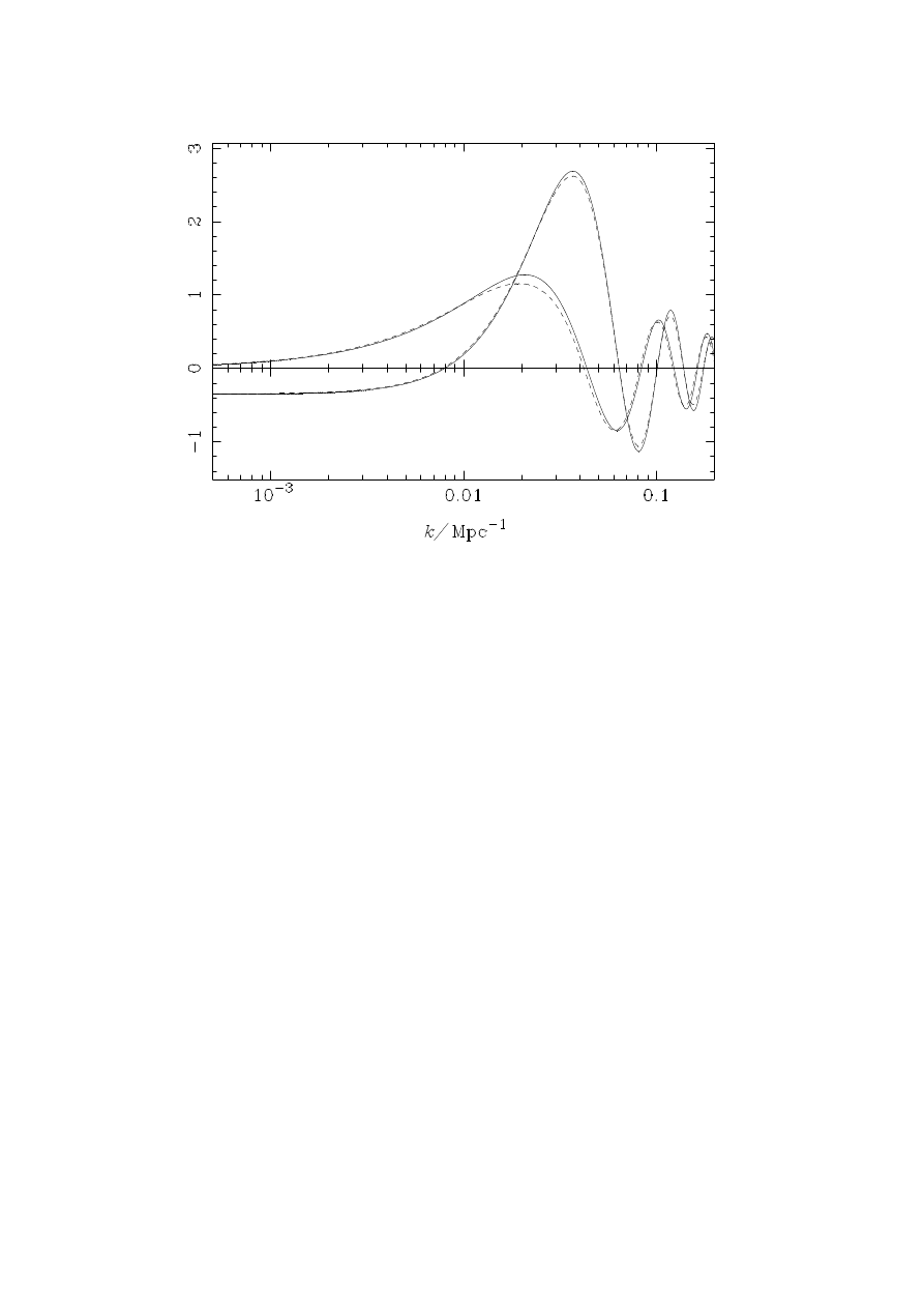
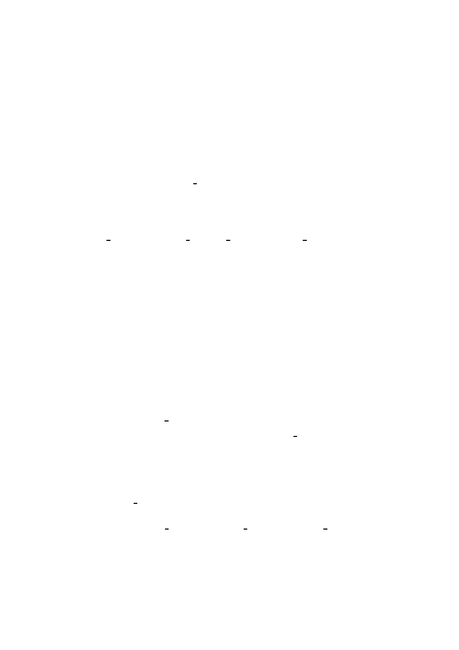
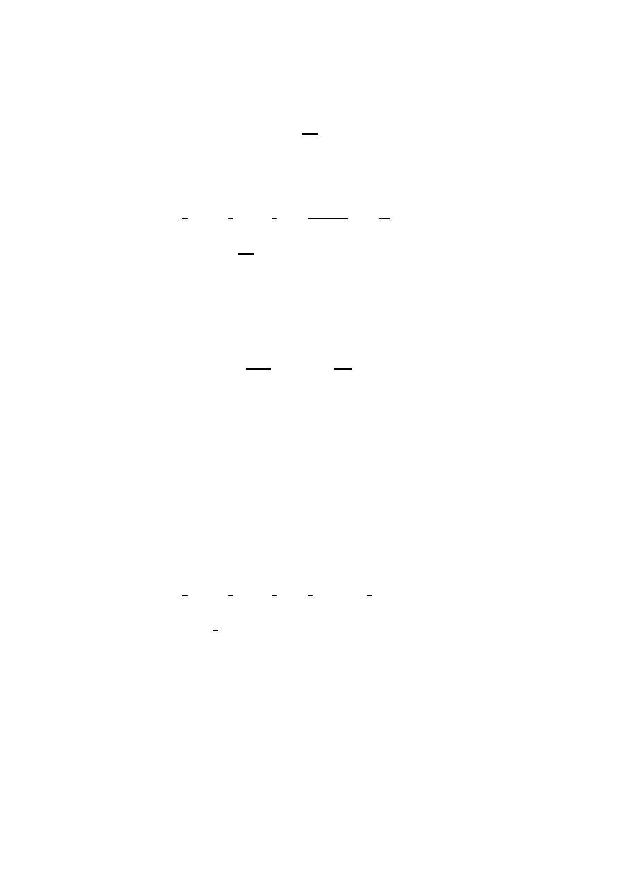
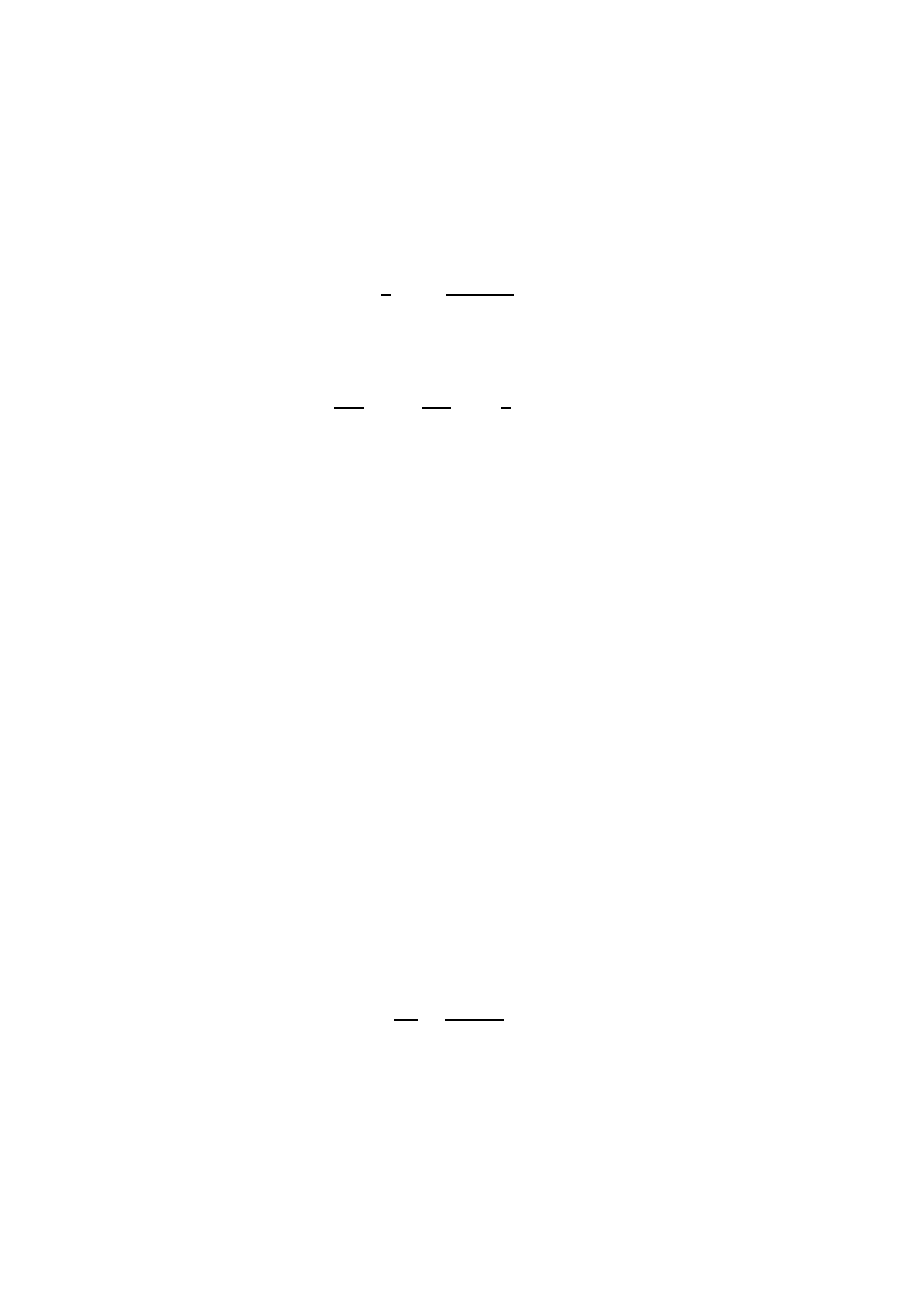
Figure 1:

Contributions to the CMB temperature anisotropy from the conditions on

the last scattering surface (z ' 1050) in a K = 0 universe with Ω

= 1, and H

50kms

−1

Mpc

−1

. Only adiabatic scalar perturbations are considered, and Φ

is indepen-

dent of k initially (so that we are plotting transfer functions). The curves should be mul-
tiplied by the initial Φ

to give the actual conditions on the last scattering surface. The

solid lines are calculated from Eq. (3.17); the “monopole” contribution (negative on large
scales) is X

(γ)

/4 + S( ˙σ

− w

)/k, and the “dipole” contribution (positive on large scales) is

−σ

−v

(b)

. The dashed lines are given by the approximate expression (4.7); the “monopole”

contribution (negative on large scales) is X

(γ)

/4−X

(b)

/3−Φ

/3+ 2H

−1

˙Φ

/3+ 2H

−2

/9,

and the “dipole” contribution is 2H

−1

(Φ

+ H

−1

˙Φ

)/3. The small discrepancy between

the solid and dashed curves is due to the small but non-zero values of ρ

(γ)

/ρ and ρ

(ν)

/ρ at

last scattering.

In Fig. 1 we plot the first two summands in equations (3.17) and (4.7) as a

function of k, with S = 1 at the present, in a K = 0 universe, in the limit Ω

= 1,

where Ω

is the present-day baryon density in units of the critical density. We take

= 50kms

−1

Mpc

−1

and consider adiabatic perturbations with only the fastest

growing mode present. At early times, we take Φ

to be independent of k. The actual

conditions on the last scattering surface are obtained from the transfer functions of
Fig. 1 by multiplying by the initial values of Φ

(which are Gaussian random variables

in most inflationary theories). The gauge-invariant variables on the last scattering
surface are obtained from an accurate Boltzmann code employing covariant, gauge-

invariant variables, with adiabatic initial conditions [7]. The agreement between the
approximate expression (4.7) and the “exact” expression (3.17) is good over the full
range of k depicted. The small discrepancy between the sets of curves is due to the
small but non-zero values of ρ

(γ)

/ρ and ρ

(ν)

/ρ on the last scattering surface (which

is located at z ' 1050 in this model).

On large angular scales (small k), the “monopole” terms dominate the CMB

anisotropy, giving the familiar Sachs-Wolfe plateau for a scale-invariant spectrum
of initial conditions. On smaller angular scales the “monopole” term oscillates in
k due to the coherent acoustic oscillations in the photon-baryon plasma that occur
for modes inside the (sound) horizon. These oscillations, along with the oscillations
in the “dipole” on small scales, determine the structure of the Doppler peaks in the
CMB power spectrum. For adiabatic perturbations in a K = 0 universe, the first
zero in the “monopole” contribution to the anisotropy (the initially lower curves
in Fig. 1) occurs where H

≈

√

(2/3). This follows from Eq. (4.7), the fact that

initially adiabatic perturbations are still adiabatic at last scattering on such scales
(see Fig. 2), and the approximate stationarity of the potential Φ

in the matter

dominated era of a K = 0 universe. This effect was noted recently by Ellis and
Dunsby [6], and was also discussed by Hu and Sugiyama [14]. Ellis and Dunsby
suggested that this zero in the “monopole” contribution should be observable as a
zero in the CMB power spectrum on angular scales ' 50

. However, as noted by Hu

and Sugiyama and evident in Fig. 1, the “dipole” contribution is already significant
on these angular scales, with its first maximum occurring close to the zero in the
“monopole”. This tends to wash out the zero (actually a dip once the k modes are
summed over) in the power spectrum, as shown by Hu and Sugiyama [14] in their
Fig. 4.

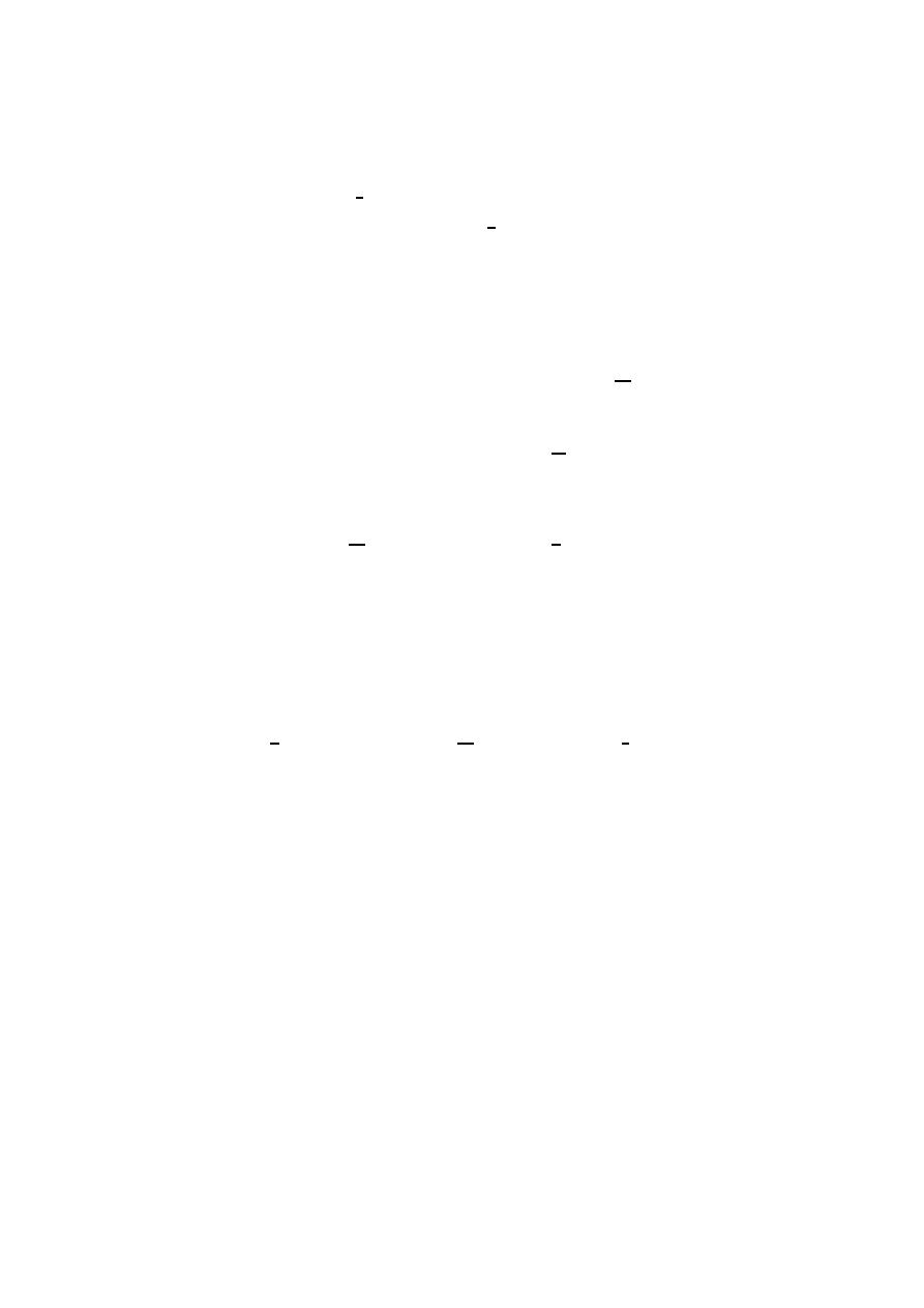
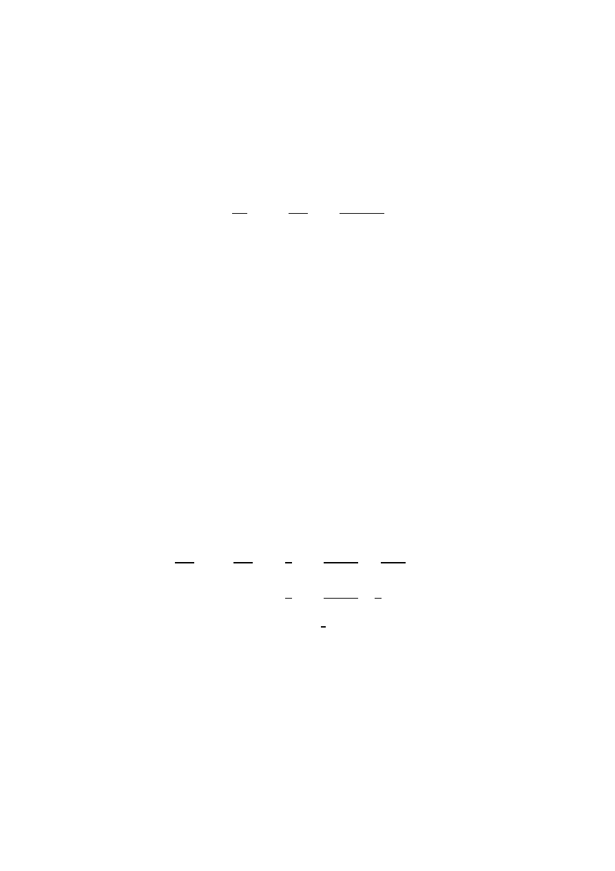
In Fig. 2 we plot the individual contributions to the CMB anisotropy in the

baryon dominated limit from equation (4.7). On large scales (small k), the domi-
nant contribution is from the usual Sachs-Wolfe term −Φ

/3. The effect of entropy

perturbations is negligible on large scales since the baryon-photon fluid is still tightly-
coupled at last scattering on these scales, and our initial conditions are adiabatic.
However, on small scales the entropy perturbations add coherently with the term
2H

−2

/9 to reduce the “monopole” contribution to the anisotropy. These terms

along with the “dipole” term determine the structure of the Doppler peaks.

We introduced X

(b)

into Eq. (4.3) to show explicitly the contribution from entropy

perturbations at last scattering, and to facilitate comparison with other results in
the literature. However, this decomposition into an entropy perturbation term and
terms involving the potential Φ

is rather unnatural, and can be replaced by an

expression which allows a more physical interpretation of the temperature anisotropy
on intermediate and small scales. We use Eq. (4.1) to eliminate X

(b)

and choose u

coincide with the baryon velocity (v

(b)

= 0; if the universe is not baryon dominated

at recombination, then the energy-frame should be employed instead of the baryon-

Figure 2:

Approximate contributions to the CMB temperature anisotropy from the con-

ditions on the last scattering surface (z ' 1050) in a K = 0 universe with Ω

= 1, and

= 50kms

−1

Mpc

−1

. Only adiabatic scalar perturbations are considered. On large scales

the usual Sachs-Wolfe term (dotted line) −Φ

/3 dominates. For adiabatic initial condi-

tions, the effect of entropy perturbations (dashed-dotted line) is only important on small
scales where the tight-coupling approximation ceases to hold and adiabaticity is broken.
The coherent sum of the entropy perturbations and the term 2H

−2

/9 (solid line), as

well as the “dipole” term 2H

−1

(Φ

+ H

−1

˙Φ

)/3 (dashed line) determine the structure of

the Doppler peaks.

frame):

1
4

(γ)

( ˙σ

− w

) →

1
4

(γ)

−

1
3

−

κρ

˙Φ

(4.8)

where ¯

(γ)

is the harmonic expansion coefficient of the spatial gradient of the photon

energy density in the energy-frame. This result actually holds in the energy-frame
of any model that is matter dominated at last scattering, and so includes standard
CDM and variants. We see that in a K = 0 universe, which is matter dominated
at recombination, the “monopole” contribution to the anisotropy consists of the
Sachs-Wolfe term, −Φ

(k)

/3, which is dominant on large scales, a term ¯

(γ)

(k)

arising from inhomogeneity of the radiation temperature in the energy-frame, which
is important on intermediate and small scales, and the small term 2H

−1

˙Φ

(k)

arising from non-stationarity of the potential at last scattering. Since the last scat-

tering surface is well approximated by a surface of constant radiation temperature,
the spatial gradient of the radiation energy density, in the energy frame, across the
last scattering surface describes a distortion of the last scattering surface relative to
the surfaces of simultaneity of the energy-frame (which are defined by the average
motion of all matter in the universe). The distortion of the last scattering surface
causes photons to incur extra redshift, due to the expansion of the universe, during
propagation from last scattering to the point of observation.

Finally, if we consider initially adiabatic perturbations in a K = 0 baryon domi-

nated universe on large enough scales that entropy perturbations may be neglected,
we may replace ¯

(γ)

/4 by the spatial gradient of the baryon energy density in the

baryon-frame, ¯

(b)

/3. Replacing Φ

with 3H

(b)

/2 (from the constraint (4.1) with

K = 0) and neglecting terms involving ˙Φ

, we obtain the covariant equivalent of

Panek’s result [10]:

(δ

(e))

1
3

(b)

1 −

3
2

2
k

(k)

(b)

(k)
a

(4.9)

Comparison with the Sachs-Wolfe Result

It is instructive to compare the preceding analysis with the original calculation of
Sachs and Wolfe [1]. Assuming that the radiation is nearly isotropic in the frame of
the baryons at last scattering, the temperature of the radiation at R (in the baryon-
frame) is given in terms of the radiation temperature at the point A in the last
scattering surface as

1 + z

(5.1)

where the redshift z along the null geodesic connecting A and R is given by [1]

1 + z =

1 −

1
2

∂

+ 2∂

dη

(5.2)

where S

≡ S(η

) is the background scale factor at R and similarly for S

, h

µν

the metric perturbation in the comoving gauge (with h

= 0), η is conformal time,

and e

(i = 1, 2, 3) is the direction of photon propagation in the background model.

Differencing the temperature between two directions on the sky we find

∆T

∆S

1
2

∆

∂

+ 2∂

dη

(5.3)

where (∆M)

≡ (M)

−(M)

. The (∆S)

term on the right-hand side of Eq. (5.3) is

gauge-dependent (first-order gauge transformations of the form η 7→ η + f(x

)/S(η),

which preserve the gauge-conditions implicit in Eq. (5.2), move the field S around in

the real universe), while the term (∆T )

is gauge-invariant. It follows that the sum

of the first two terms on the right-hand side of Eq. (5.3) is also gauge-dependent. (A
compensating gauge-dependence in the integral term preserves the necessary gauge-
invariance of (∆T )

.) This sum may be expressed in terms of the gauge-dependent

photon density perturbation δ

(γ)

, defined by

1
4

(γ)

≡

T − T

(0)

(5.4)

where T

(0)

≡ T

(0)

(η) is the background radiation temperature. Using the constancy

of T

(0)

S, we find

∆T

∆S

1
4

∆(δ

(γ)

)

(5.5)

The significance of this result is that it is a first-order quantity. To evaluate ∆(δ

(γ)

)

to first-order, we need only locate the last scattering surface to zero-order, since lo-
cating the last scattering surface correctly amounts to a first-order displacement in
a first-order quantity. The implicit choice made by many authors is to evaluate
Eq. (5.5) on the background last scattering surface (over which η is constant). With
this choice ∆S and ∆T

(0)

are both equal to zero, and trivially we obtain the result

∆(δ

(γ)

)

evaluated on the background last scattering surface. Note that Sachs and

Wolfe [1] explicitly made this choice, although they also made the (gauge-dependent)
assumption that the radiation temperature was constant on the background last scat-
tering surface. Although it is certainly necessary to locate last scattering correctly
to calculate ∆(T )

and ∆(S)

separately, this is not true for the difference ∆(T S)

which is all that is required for CMB calculations. Physically, this effect arises from
the compensation effect: the extra redshift along a given direction due to the differ-
ence between the scale factor on the true last scattering surface and at the point of
intersection of the geodesic with the background (zero-order) last scattering surface
cancels out the difference in temperature between the same points on the real and
true last scattering surface. Note that such problems do not arise in the kinetic the-
ory calculation of Section 3, since the optical depth (which determines the position
of the last scattering surface) multiplies only first-order variables, and so is needed
only to zero-order.

The term ∆(δ

(γ)

)

/4 is often omitted from Sachs-Wolfe type analyses (for exam-

ple, [15]), effectively being absorbed into a (direction-dependent) “expected” tem-
perature, ¯

T ≡ T

(see [2, 10] for alternative choices). Along with the observed

temperature T

, this defines a first-order temperature variation δT /T by

δT

≡

− ¯

(5.6)

This should not be confused with the gauge-invariant temperature fluctuation from
the mean δ

(e), used in the rest of this paper. The quantity δT /T is gauge-dependent

through the gauge-arbitrariness in the scale factor S. Differencing between two
directions on the sky, one finds

∆ (δT /T )

= ∆

∂

+ 2∂

dη

(5.7)

Of course, this result is entirely equivalent to Eq. (5.3), one needs only the result

∆

δT

∆T

−

∆(T S)

(T S)

(5.8)

which follows from the definition of ¯

T . This appears to be the step where confusion

sometimes arises in Sachs-Wolfe type analyses, with authors comparing the gauge-
dependent δT /T with the results of observation, instead of the physically relevant
(∆T /T )

(or δ

(e) which is easily derived from the former). As noted in [2], it is

not enough just to difference δT /T ; in general, the result will not be gauge-invariant
and will not include the contribution from δ

(γ)

at last scattering.

Finally, we demonstrate how the gauge-invariant contribution ¯

(γ)

(k)

/4 to the

anisotropy arises in the Sachs-Wolfe calculation. If we approximate the (vorticity-
free) baryon motion as being geodesic through recombination to the present, we
can choose a comoving gauge with h

= 0 (the synchronous gauge, in which the

surfaces of constant η are surfaces of simultaneity for the baryons). The result given
in Eq. (5.3) (with h

= 0) still holds in this gauge, and the conformal time η satisfies

∇

η = u

(b)

/S(η), where u

(b)

is the baryon velocity. It follows that the background

scale factor satisfies

(3)

∇

S = 0 and ˙

S = ∂

S/S = θS/3 + O(1), where θ = ∇

(b)

is the covariant expansion of the baryon-frame. With this gauge-condition, we have
removed the gauge-freedom to perform the transformation η 7→ η + f(x

)/S (the

gauge-condition

(3)

∇

η = 0 forces f (x

) to be a constant), with the result that ∆S/S

is gauge-invariant. Under these conditions, we may express the first two terms on
the right-hand side of Eq. (5.3) in terms of covariant, gauge-invariant variables as
follows:

∆T

∆S

1
4

∇

(γ)

+ 4

∇

1
4

∇

(γ)

4
3

θu

(b)
a

∆

1
4

(γ)

(k)

(5.9)

where A and B are the points of intersection of the two geodesics through the
observation point R with the last scattering surface, dx

lies in the last scattering

surface (dx

(b)

= O(1)), and we have replaced 3 ˙S/S by the covariantly defined θ

which is correct to the required order. In this manner, we recover the ¯

(γ)

(k)

contribution to the temperature anisotropy.

Conclusion

Starting from a covariant and gauge-invariant formulation of the Boltzmann equa-
tion, we have derived a new expression for the CMB temperature anisotropy under
the instantaneous recombination approximation, valid for scalar perturbations in
open, closed and flat universes. Our expression uses only covariantly-defined vari-
ables, and is manifestly gauge-invariant. The result is more useful in multicomponent
models with scalar perturbations than earlier covariant results [6, 8, 9]. In the case
of a universe which is baryon-dominated at recombination, we find a simple expres-
sion for the anisotropy which corrects a similar result by Dunsby [9]. By making
use of numerical solutions to the perturbation equations, we have discussed the con-
ditions on the last scattering surface and their contributions to the characteristic
features of the CMB power spectrum. We ended with a discussion of the original
Sachs-Wolfe calculation for the temperature anisotropy. We have discussed why it
is not necessary to locate accurately the last scattering surface in such calculations
(because of the compensation effect), and how the extra term in the Sachs-Wolfe
calculation, reported recently by Ellis and Dunsby [6], is missed in many calcula-
tions which employ a gauge-dependent “expected temperature”, since the angular
dependence of this temperature is often overlooked. For a universe which is matter
dominated at recombination, but not necessarily adiabatic, the extra term is the
spatial gradient of the radiation energy density in the energy-frame, ( ¯

(γ)

(k)

/4)

For models with isothermal surfaces of last scattering, this inhomogeneity describes
a distortion of the last scattering surface relative to the surfaces of simultaneity
of the energy-frame. The extra redshift incurred by this distortion is a significant
component of the temperature anisotropy on intermediate and small scales.

References

[1] R. K. Sachs and A. M. Wolfe, Astrophys. J. 147, 73 (1967).

[2] W. R. Stoeger, C.-M. Xu, G. F. R. Ellis, and M. Katz, Astrophys. J. 445, 17

(1995).

[3] J. M. Bardeen, Phys. Rev. D 22, 1882 (1980).

[4] G. F. R. Ellis and M. Bruni, Phys. Rev. D 40, 1804 (1989).

[5] G. F. R. Ellis, J. Hwang, and M. Bruni, Phys. Rev. D 40, 1819, (1989).

[6] G. F. R. Ellis and P. K. S. Dunsby, in Current Topics in Astrofundamental

Physics

, edited by N. S´anchez (Kluwer Academic, Dordrecht, 1998).

[7] A. D. Challinor and A. N. Lasenby, submitted to: Astrophys. J. (unpublished).

[8] A. D. Challinor and A. N. Lasenby, in Current Topics in Astrofundamental

Physics

, edited by N. S´anchez (Kluwer Academic, Dordrecht, 1998).

[9] P. K. S. Dunsby, Class. Quantum Grav. 14, 3391 (1997).

[10] M. Panek, Phys. Rev. D 34, 416 (1986).

[11] G. F. R. Ellis, D. R. Matravers, and R. Treciokas, Ann. Phys. 150, 455 (1983).

[12] S. W. Hawking, Astrophys. J. 145, 544 (1966).

[13] M. Bruni, P. K. S. Dunsby, and G. F. R. Ellis, Astrophys. J. 395, 34 (1992).

[14] W. Hu and N. Sugiyama, Astrophys. J. 444, 489 (1995).

[15] T. Padmanabhan, Structure formation in the universe (Cambridge University

Press, Cambridge, England, 1993).