
University of Alberta
Static detection and identification of X86 malicious
executables: A multidisciplinary approach
by
Zhiyu Wang
A thesis submitted to the Faculty of Graduate Studies and Research
in partial fulfillment of the requirements for the degree of
Master of Science
Department of Computing Science
c
Zhiyu Wang
Fall 2009
Edmonton, Alberta
Permission is hereby granted to the University of Alberta Libraries to reproduce single
copies of this thesis and to lend or sell such copies for private, scholarly or scientific
research purposes only. Where the thesis is converted to, or otherwise made available in
digital form, the University of Alberta will advise potential users of the thesis of these
terms.
The author reserves all other publication and other rights in association with the
copyright in the thesis, and except as herein before provided, neither the thesis nor any
substantial portion thereof may be printed or otherwise reproduced in any material form
whatever without the author’s prior written permission.

Examining Committee
Mike H. MacGregor, Computing Science
Mario A. Nascimento, Computing Science
Raymond Patterson, Alberta School of Business
GuoHui Lin, Computing Science

This thesis is dedicated to my parents and lovely wife.
iii

Thesis advisor
Author
Mike H. MacGregor,
Zhiyu Wang
Abstract
In this thesis, we propose a novel approach to detect malicious executables in the
network layer using a combination of techniques from bioinformatics, data mining and
information retrieval. This approach requires translating malicious code into genome-
like representations. Based on their “genetic” formats, we can easily extract features
by constructing families for known malicious code using data mining algorithms.
These features then can be stored in a router or an another device in the network to
measure the similarity between payloads and extracted features. Once the similarity
is over a threshold, the security device can block the entire session and report an
alert before the threat reaches the intended host(s). Further more, attacks can be
identified based on their features and the families where these features come from.
Ultimately, our experiments showed that 95% accuracy of detection is possible with
an identification rate of 83%.
iv
Contents
Dedication . . . . . . . . . . . . . . . . . . . . . . . . . . . . . . . . . . . .
iii
Abstract . . . . . . . . . . . . . . . . . . . . . . . . . . . . . . . . . . . . .
iv
Table of Contents . . . . . . . . . . . . . . . . . . . . . . . . . . . . . . . .
vi
List of Figures . . . . . . . . . . . . . . . . . . . . . . . . . . . . . . . . . .
vii
List of Tables . . . . . . . . . . . . . . . . . . . . . . . . . . . . . . . . . . viii
Acknowledgments . . . . . . . . . . . . . . . . . . . . . . . . . . . . . . . .
ix
1
Definitions of detection and identification . . . . . . . . . . . . . . . .
2
. . . . . . . . . . . . . . . . . . . . . . . . . . . .
3
Signature based methods . . . . . . . . . . . . . . . . . . . . .
3
Heuristic methods . . . . . . . . . . . . . . . . . . . . . . . . .
4
Distributed system . . . . . . . . . . . . . . . . . . . . . . . .
5
Motivation and challenges . . . . . . . . . . . . . . . . . . . . . . . .
6
Motivation . . . . . . . . . . . . . . . . . . . . . . . . . . . . .
6
. . . . . . . . . . . . . . . . . .
7
. . . . . . . . . . . . . . . . . . . . . . . . . . .
9
10
Binary-based detection . . . . . . . . . . . . . . . . . . . . . . . . . .
11
Instruction-based detection . . . . . . . . . . . . . . . . . . . . . . . .
13
Hybrid detection . . . . . . . . . . . . . . . . . . . . . . . . . . . . .
14
17
Malicious attacks . . . . . . . . . . . . . . . . . . . . . . . . . . . . .
18
Clustering algorithms from data mining . . . . . . . . . . . . . . . . .
19
Techniques from information retrieval . . . . . . . . . . . . . . . . . .
21
Term Frequency/Inverse Document Frequency . . . . . . . . .
21
v
Contents
vi
Cosine similarity . . . . . . . . . . . . . . . . . . . . . . . . .
22
Alignment algorithms from bioinformatics
. . . . . . . . . . . . . . .
23
Performance measurement . . . . . . . . . . . . . . . . . . . . . . . .
25
Malicious code detection and identification
27
Data preparation . . . . . . . . . . . . . . . . . . . . . . . . . . . . .
27
Disassembly . . . . . . . . . . . . . . . . . . . . . . . . . . . .
28
Opcode grouping . . . . . . . . . . . . . . . . . . . . . . . . .
28
s-opcode sequence transformation . . . . . . . . . . . . . . . .
29
Clustering . . . . . . . . . . . . . . . . . . . . . . . . . . . . . . . . .
30
Distance measurement . . . . . . . . . . . . . . . . . . . . . .
31
Clustering algorithm . . . . . . . . . . . . . . . . . . . . . . .
33
. . . . . . . . . . . . . . . . . . . . . . . . . . . .
35
Applying features to the problems of detection and identification . . .
39
. . . . . . . . . . . . . . . . . . . . . . . . . . . . . . . . .
40
Experiments and Performance Evaluation
41
Datasets . . . . . . . . . . . . . . . . . . . . . . . . . . . . . . . . . .
41
Experiment setup and simulation . . . . . . . . . . . . . . . . . . . .
42
Results . . . . . . . . . . . . . . . . . . . . . . . . . . . . . . . . . . .
43
Parameter selection . . . . . . . . . . . . . . . . . . . . . . . .
43
Analysis . . . . . . . . . . . . . . . . . . . . . . . . . . . . . .
46
Experiments against the training set . . . . . . . . .
46
Experiments against the entire dataset . . . . . . . .
56
58
Limitations . . . . . . . . . . . . . . . . . . . . . . . . . . . . . . . .
59
Future work . . . . . . . . . . . . . . . . . . . . . . . . . . . . . . . .
59
65
66
B numerical experimental results
74
List of Figures
The hybrid model explanation for training phase and testing phase
from Masud et al. [27]. . . . . . . . . . . . . . . . . . . . . . . . . . .
15
Terminology explanation from Ester et al. [13]. . . . . . . . . . . . . .
21
Comparison between global and local alignments . . . . . . . . . . . .
24
Binary to s-opcode sequence transformation . . . . . . . . . . . . . .
29
Sliding window used to retrieve length k term list. . . . . . . . . . . .
32
Result from a complete hierarchical clustering algorithm. . . . . . . .
34
Feature list size. . . . . . . . . . . . . . . . . . . . . . . . . . . . . . .
37
Processes of our approach . . . . . . . . . . . . . . . . . . . . . . . .
40
Sorted average distance to k nearest neighbors.
. . . . . . . . . . . .
45
Individual segment examination . . . . . . . . . . . . . . . . . . . . .
48
Individual segment examination with merged features . . . . . . . . .
50
Double segments examination . . . . . . . . . . . . . . . . . . . . . .
52
Double segments examination with merged features . . . . . . . . . .
53
Varying number of segments examined . . . . . . . . . . . . . . . . .
54
Individual segment examination with varied alignment thresholds . .
55
Double segments examination with varied alignment thresholds . . . .
56
vii
List of Tables
Single character representation of opcode categories. . . . . . . . . . .
30
Adjusted score matrix. . . . . . . . . . . . . . . . . . . . . . . . . . .
33
Multiple alignment that has common subsequences. . . . . . . . . . .
36
The content of the feature list changes by varying the threshold refer-
ring to Figure 4.4. . . . . . . . . . . . . . . . . . . . . . . . . . . . . .
38
Overall accuracy of detection. . . . . . . . . . . . . . . . . . . . . . .
47
OAD using double segments examination . . . . . . . . . . . . . . . .
51
A.1 Opcode grouping . . . . . . . . . . . . . . . . . . . . . . . . . . . . .
73
B.1 Numerical results for individual segment examination referring to Fig-
ure 5.2. . . . . . . . . . . . . . . . . . . . . . . . . . . . . . . . . . . .
74
B.2 Numerical results for individual segment examination using the merged
feature list referring Figure 5.3. . . . . . . . . . . . . . . . . . . . . .
74
B.3 Numerical results for double segments examination referring to Fig-
ure 5.4. . . . . . . . . . . . . . . . . . . . . . . . . . . . . . . . . . . .
75
B.4 Numerical results for double segments examination using the merged
feature list referring to Figure 5.5. . . . . . . . . . . . . . . . . . . . .
75
B.5 Numerical results for varying the number of examining segments re-
ferring to Figure 5.6. . . . . . . . . . . . . . . . . . . . . . . . . . . .
75
B.6 Numerical results for varying classifier threshold for one segment ex-
amination referring to Figure 5.7. . . . . . . . . . . . . . . . . . . . .
76
B.7 Numerical results for varying classifier threshold for double segments
examination referrring to Figure 5.8.
. . . . . . . . . . . . . . . . . .
76
viii

Acknowledgments
First of all, I would like to thank my supervisors, Dr. Mike MacGregor and Dr.
Mario Nascimento. Without their extensive support and patience, this work would
be impossible for me. I would also like to thank faculty members, Dr.Guohui Lin
and Dr.Joerg Sander, for their generous assistance. Thanks to Sunil Ravinder for his
comments during the meetings.
I really appreciate the financial support from the Computing Science Department
at the University of Alberta, and from NSERC.
Finally, I would like to thank my parents and wife for their long-term under-
standing and love.
ix

Chapter 1
Introduction
Malicious executables are programs that perform malevolent functions. They
hide somewhere in the computer system, infect other benign files and execute harm-
ful operations, such as destroying private data, consuming physical resources, pro-
viding unauthorized remote access to the system, stealing sensitive information and
so on. Billions of dollars are lost every year due to damage from computer viruses
alone. Therefore, detecting and identifying malicious executables play a crucial role
in protecting computer systems.
The problem of malicious executables has become a serious security threat, espe-
cially with the growth of Internet usage. Networking provides not only an easy way
to communicate between hosts, but it also provides a convenient tunnel to widely
and quickly propagate dangerous attacks. Since the creation of the first computer
virus in the mid-1980s, the number of malicious programs has been increasing very
fast every year. Malicious code can now reach all aspects of the computer system.
The majority of the operating system market is taken by the series of Microsoft
Windows
R
operating systems. These operating systems are highly popular, but
they still have a large number of systemic holes that are vulnerable to attacks. Thus,
the majority of malicious executables aim at Windows operating systems and appli-
1

Chapter 1: Introduction
2
cations. These programs, both malicious and benign, all run on the Intel processor
that use the X86 instruction set architecture. Systemic defects demand some defense
mechanisms to secure the system.
Currently, Windows-based security systems, anti-virus and internet security soft-
ware, mainly use signatures from known malicious executables composed of binary
sequences to prevent threats. These systems can only detect malicious executables,
whose signatures were previously identified and are stored in a database. In this
thesis, we aim at improving the effectiveness of detecting and identifying malicious
X86 executables. For that, we apply techniques from multiple disciplines to packet
classification in the network layer of computer networking.
1.1
Definitions of detection and identification
Detecting malicious executables is an interesting and important problem. Given
dangerous executables, the detection problem is how to effectively discover threats to
prevent system damage. Currently, dynamic analysis and static analysis are the main
detection techniques. Dynamic detection monitors potential malicious attacks during
their execution to observe abnormal behaviors. In contrast, static detection analyzes
the properties of malicious attacks before their execution. Bergeron et al. [4] argue
that static analysis has some advantages over dynamic analysis: it allows exhaustive
analysis; it gives a verdict; and there is no run-time overhead. Probably because of
these benefits, static analysis has been adopted widely and many static automated
systems have been built using feature extraction techniques in recent years [17, 24,
38, 41], though all have their limitations. Feature extraction is the core component of
these systems, and it is also a complicated task requiring a combination of different
data processing algorithms. Although features provide important information to
detect malicious executables, it is still difficult to completely understand various
attacks. For this reason, dynamic analysis can be an accessorial supplement used to

Chapter 1: Introduction
3
further improve the detection rate. Both static and dynamic analysis are helpful.
But we concentrate on static detection in this thesis.
While many detection techniques have been proposed, the problem of identifying
malicious executables has not been given the attention it deserves. Given harmful
code, the identification problem is how to correctly recognize attacks and classify
them into possible families. Currently, human experts are involved in the process of
identifying and classifying new attacks. No automated system from our knowledge
has been released to provide suggestions to label new attacks. We also aim at this
problem beside the problem of detection. Algorithmic identification can offer us an
opportunity for building a system with the ability to identify and classify previously
unknown malicious executables automatically.
1.2
Previous Solutions
The ability to detect and identify malicious executables has evolved relatively
slowly. Signature-based methods are still being commercially used; even though
they cannot help detecting new attacks. New content-based solutions have been
proposed, but they have not been implemented in real-time. Distributed security
schemes provide a great potential to subvert the architecture of current anti-virus
software. Since no work has addressed the problem of automated identification, in
this section, we present only a brief introduction to different detection methods and
their pros and cons.
1.2.1
Signature based methods
The first attempts to detect malicious executables (mainly viruses) were based
on signatures. These approaches require the use of experts to manually extract
signatures from destructive samples. These signatures are used to detect possible

Chapter 1: Introduction
4
incoming attacks. However, signature extraction with human involvement is time
consuming. Therefore, Kephart and Arnold [23] introduced an automatic method
to extract signatures from samples of known viruses to remove the need for human
experts. This has made the development of automated security systems possible.
In fact, automated signature-based detection has been adopted to build commercial
anti-virus software. The success of signature-based techniques has shown that they
work very well for detecting known malicious executables, but they fail to prevent
new attacks. After damage reports of new attacks are issued, the executables are sent
to labs to analyze their functionalities. When the key binary sequences are found,
client-side security programs have to update their malicious signature databases.
According to Fitzgerald [15], “2007’s total doubled the number of signatures F-
Secure had built up over the previous 20 years.” From this argument, it is obvious
that lack of signatures for new attacks reduces the effectiveness of current anti-virus
systems every year.
1.2.2
Heuristic methods
In academia, it has been recognized that the capabilities of signature-based se-
curity systems have faded away [2, 17, 24, 27, 33, 38, 41]. In order to overcome
the shortcomings of signature-based solutions, some open problems about computer
virus research were presented by White [39]. One of the problems is to develop
heuristic techniques for detection. Actually, static analysis is a heuristic technique,
where researchers analyze the features of malicious executables. These features are
the core representations of the malicious executables. By using these features, we
can inspect new attacks in a heuristic approach without exact signature matching.
Unlike binary sequences, features have varied formats, and there are many different
ways to extract features.
Byte patterns were one of the first features to be considered. Using an n-gram

Chapter 1: Introduction
5
model [26], byte sequences in hex format are broken into multiple short subsequences,
each with a length of n. Then the frequency of each unique n-gram subsequence is
counted in order to determine whether it qualifies as a feature or not. The feature
list may be pruned based on other constraints. A classifier is trained later using
these features to label new malicious executables. Many researchers [2, 17, 24] use
byte patterns as features to guide their classifiers, but there are problems with this
type of the feature. All we can get from byte patterns are binary numbers. In this
case, we have no knowledge of the malicious code at all. We need to use the features
to understand the information hidden behind the binary digits.
Recently, the emphasis of feature extraction has shifted from binary analysis to
content analysis, that is an analysis of assembly code. Reverse engineering techniques
are involved in the process of content analysis. First of all, malicious executables
are translated from binaries into low-level assembly code. This facilitates a better
understanding of the functionality of the malicious executables. Depending on the
contents of the assembly code, there are many types of features that may be ex-
tracted. Bergeron et al. [4] chose to use control-flow graphs of API function calls
as features. Zhang et al. [41] applied the n-gram model to the sequences of API
functions to refine their features. Here, the API is the application programming
interface to the operating systems. A more novel approach is from Masud et al. [27].
They combined three types of features consisting of DLL (Dynamic Link Library)
functions, assembly n-gram features and binary n-gram features, to build a hybrid
model to discover new attacks. Besides these examples, there are many other types
of features. In this thesis, we select opcode sequences to be our features.
1.2.3
Distributed system
All previous solutions to the problem of detecting malicious executables are iso-
lated to run on a single host. Every client host, as a single entity, installs some

Chapter 1: Introduction
6
security systems to protect itself. Recently, some commercial companies and re-
searchers have been proposing a distributed approach. This distributes the task of
detecting and identifying malicious executables across the whole network. An anti-
virus company, Rising
R
, has already deployed its defense mechanism called “cloud
security plan” using cloud computing. In their scheme, each client host becomes a
sensor to detect abnormal behaviors and risky files. Identified malicious targets are
sent to a central node for further processing. After analyzing them, solutions are
returned to the source and are shared with all end users immediately. In this case,
client hosts are not separated entities any more. They only carry small connected
portions of the entire security system to protect all the users. Unfortunately, the
current version of cloud-based security is aimed at trojan horses only.
1.3
Motivation and challenges
In the prior sections, we have briefly described the strategies to solve the problem
of detecting malicious attacks. Signature-based systems perform poorly against new
attacks, and recent research only focuses on the detection of destructive code. We
then asked ourselves the question: can we find a technique to effectively detect
new attacks and also identify them? To address the problems of both detection and
identification, we propose a approach using a combination of techniques from multiple
disciplines to statically analyze known malicious attacks, in order that extracted
features can be used to detect and identify both previously known and unknown
malicious executables.
1.3.1
Motivation
From our observation, some behaviors of malicious executables are similar to bio-
logical organisms, such as diseases and viruses. In some circumstances, attacks break

Chapter 1: Introduction
7
out, self-replicate and propagate just like diseases and viruses. Usually, biologists
analyze organisms using their DNA/RNA materials [5]. Inspired from biological
genetic composition, we could analyze malicious executables using their simulated
“genetic” representations. A new discipline of computing science, bioinformatics,
has advanced biological analysis especially in the area of genome analysis. What we
can do is to treat binary executables as “genomes”. Important features obtained
from binary “genomes” could be the “genes”. In order to find them, we can ana-
lyze binary executables using their simulated “protein” sequences representations.
Currently, researchers have already applied bioinformatics techniques to intrusion
detection [8, 36]. Its algorithms combined with other techniques could be employed
to address the problem of detecting and identifying new malicious attacks as well.
Detection using content analysis can potentially achieve higher accuracy than bi-
nary analysis. However, existing systems only focus on detecting malicious executa-
bles, they do not address the problem of identification. Commercially, new attacks
must still be sent to human experts for identification and classification. Therefore,
we believe a high detection rate is no longer enough. The next questions we have
to ask ourselves are: what kinds of functionalities make programs virulent? Which
families do they belong to? Security systems should be able to provide some advice
about answering these questions.
1.3.2
Challenges and opportunities
Our challenge is to choose a proper format to represent characteristics of mali-
cious executables. Byte sequences are one choice. However, in order to bypass de-
tection through binary features, programmers of malicious programs try to disguise
their work. For example, they may add extra instructions, or extend instruction
sequences into longer equivalent sequences. Therefore, binary/hex representation by
itself is not sufficient. At some level, similar malicious operations must have similar

Chapter 1: Introduction
8
instruction sequences. If we reverse binary executables into assembly code, there
must be some similar subsequences of instructions existing in all related malicious
attacks, and these subsequences should also be unique compared to other types of
attacks. Thus, the hypothesis in this thesis is that: there exists at least one unique
common instruction subsequence in every member of the same malicious family. In
other words, benign executables should not contain any of these characteristic in-
struction sequences. In order to test this hypothesis, we encounter the following
challenges:
• To choose a proper representation to describe malicious executables. Binary/byte
patterns, API functions, control-flow graphs and other types listed previously
can all be used to represent malicious executables, but which type is more
appropriate to our hypothesis?
• To algorithmically construct the families for malicious executables. To our
knowledge, no solution has been proposed to automatically cluster malicious
attacks, i.e., they are classified manually by human experts. If our clustering
approach works, then we have a solution or can at least provide some sugges-
tions for algorithmically grouping malicious attacks.
• To extract features from each family, because each family contains many ma-
licious members that include a large amount of information. It is difficult to
find the feature that can represent the whole family.
• How to use features and how to take advantage of them to address the problem
of detecting and identifying malicious executables.
Chapter 1: Introduction
9
1.4
Outline of the thesis
The remainder of this thesis is organized as follows. An overview of the existing
systems for detecting malicious executables is discussed in Chapter 2. Also, Chapter 3
provides the discussion about the background of some fundamental algorithms from
data mining, bioinformatics and information retrieval. In Chapter 4, we introduce the
processes of our approach, including data preparation, clustering, feature extraction
and application of features. Chapter 5 presents the details of experiments conducted
to evaluate the accuracy of our system. Finally, conclusions and suggestions for
future work are given in Chapter 6.

Chapter 2
Related work
The idea of using a signature was one of the methods used to detect malicious
executables in the early days, and papers, e.g., [11, 23] have been published about
how to extract useful signatures from computer viruses. But it has been recognized
afterwards that signatures cannot be used to protect against entirely new attacks.
Researchers now apply heuristic analysis to potential malicious executables with the
purpose of finding their essential features. In this case, data mining and information
processing techniques become important tools to address the problem of detecting
malicious executables. Features can then be employed to discover new attacks con-
taining similar characteristics. Many different types of features have been proposed
recently. Binary n-gram patterns [2, 6, 17, 24] are considered as features to examine
the binary representations of malicious code. Instruction sequences and API func-
tion calls [4, 38, 41] have also been used to inspect the contents of malicious attacks.
There are many other types of features as well, but it does not matter what kind
of features one would like to use, the ultimate goal is to build an efficient classifier
using these features to effectively and accurately detect new attacks.
In this section, we concentrate on the previous work regarding features. Binary
feature extraction is presented in Section 2.1. Instruction-level feature extraction is
10

Chapter 2: Related work
11
discussed in Section 2.2. Finally, hybrid feature extraction by combining multiple
formats of features is introduced in Section 2.3.
2.1
Binary-based detection
Malicious executables are in binary representations. The first attempt at extract-
ing features was to find characteristics directly out of plain binary/byte sequences.
Henchiri and Japkowicz used exhaustive search for unique binary n-gram sequences
to discover helpful features [17]. By fixing a length n, they count the frequencies of
different n-gram patterns, and the set of sequences with occurrence frequency over
a certain threshold is selected for the subsequent processing. Additional thresholds
such as intra-family and inter-family supports are introduced to further eliminate
redundant sequences. Given the prior knowledge of computer virus families available
from commercial anti-virus software, intra-family support is the constraint that limits
the number of appearances of a feature in members of the same family. Inter-family
support is the constraint that controls the number of occurrences of a feature in all
malicious attacks. Only the n-gram patterns satisfying all constraints are chosen as
features. These pruned features are used to evaluate their system.
After retrieving the most relevant binary n-gram sequences, Kolter and Maloof
applied various types of classifiers to the feature set, including decision tree, naive
Bayes and support vector machine [24]. First, they converted malicious executables
into hexadecimal representations. Then, an n-gram term is generated by concate-
nating n continuous (hex) bytes; However, this n-gram selection produces millions of
distinct byte sequences. In order to find the most pertinent n-gram patterns, Kolter
and Maloof chose the top 500 n-grams independent of the length n based on their
frequencies to be features. Finally, all classifiers listed above were used to evaluate
the system using the extracted n-gram features. The work done by AbouAssaleh
et al. [2] is very similar to the method from Kolter and Maloof. Using binary n-gram
Chapter 2: Related work
12
sequences, they selected the most frequent features to discover new attacks. Multiple
experiments with 3-fold cross-validation are used in order to find the optimal length
of an n-gram and the size of the feature list that can achieve the highest detection
rate. In their experiment, AbouAssaleh et al. can achieve 98% accuracy; however,
approximately two third of the data samples is required in training purposes. Now,
the number of malicious attacks increases exponentially every year. We only have
limited resources to preform the tasks of detection of identification. What we should
do is to use the minimum resources to achieve the maximum results. Therefore, we
believe using a large training set is not appropriate any more.
As we have shown in previous paragraphs, many researchers use n-gram patterns
as features in their systems, but they have to struggle with choosing the proper
length/size for both n-gram and the feature list to get the best result [2, 17, 24].
In addition to the problem of n-gram selection, Henchiri and Japkowicz in their
work have to pre-group the virus samples into families according to the results from
commercial anti-malware software [17].
In contrast to traditional classifiers trained with both sample malicious executa-
bles and benign programs, Cai et al. investigated only the profiles of benign programs
using one-class classification [6]. In their paper, they extract distinct single bytes
from benign programs as features. Principal component analysis [25] and a one-class
support vector machine are applied to benign features to evaluate the accuracy of
detecting malicious executables. This is an interesting approach to exclusively an-
alyze the benign cases; however, single-byte features cause high false positive rates.
In some circumstances, the classifier gives a roughly 70% false positive rate while the
true positive rate is around 93% . At the same time, approximately three fourths of
the data samples is required in training purposes.

Chapter 2: Related work
13
2.2
Instruction-based detection
In recent years, content-based feature extraction has become a popular technique
to detect malicious executables. Researchers now analyze attacks by disassembling
them into low-level assembly code or languages such as C and C++. The disassem-
bled code contains sequences of instructions, system calls and sub-functions; there-
fore, These assembly programs definitely provide more information about malicious
executables than binary patterns.
Wang et al. proposed the features that are instructions in the byte representa-
tion [38]. However they only examine the first byte and the first two bytes of each
four byte chunk. They believe the first byte is the opcode and the first two bytes
are mainly composed of the opcode and the first operand. Information Gain [25]
based on the frequencies of the features is applied to remove inappropriate patterns.
Naive Bayes and decision tree classifiers are used to test the performance of the sys-
tem. Their paper describes an interesting transition from binary sequences to the
content of assembly code. However, it is unreasonable for the authors to assume
every four-byte denotes an instruction because the Intel X86 instruction set contains
variable-length instructions. The use of single-byte patterns provides insufficient
support that causes a roughly 30% false positive rate while the best detection rate
is around 93%.
Zhang et al. chose the features that are generated by a controlled sliding window
through the sequences of API function calls while assuming that all viruses must
interact with a 32-bit Windows operating system [41]. They first disassemble com-
puter viruses to extract the sequences of system function calls. Then an n-gram
sliding window is applied to break the sequences into several subsequences. The
procedure of counting the frequencies of distinct n-gram subsequences is performed
during the sliding process. Only the subsequences containing abnormal behaviors
such as aggressive function calls are considered to be features. Finally, features are

Chapter 2: Related work
14
fed to a support vector machine to discover new attacks. That paper borrows the
idea from Unix intrusion detection systems of using the abnormal sequences of Unix
commands to prevent attacks.
Besides using the sequences of API function calls as the features, the use of
an instruction-flow graph with the application of automatons is also interesting.
Bergeron et al. converted instruction sequences into control-flow graphs [4].
An
instruction-flow graph using assembly code is first constructed to imitate the pro-
cesses of instruction execution. General-purpose instructions other than system func-
tion calls or sub-routine calls are removed from the graph later. Then the instruction
flow graph is simplified into a finite state machine containing only the flows of API
functions and sub-routines. At last, a verifier is used to compare the control-flow
graphs of attacks and the predefined security automata. It is easy to construct the
flows of function calls for malicious executables; however, the difficulty here is how
to build the security automata to cover various types of malicious attacks.
2.3
Hybrid detection
Both binary-based and instruction-based detections only concentrate on one type
of feature, either byte patterns or instruction sequences. Schultz et al. however used
a set of experiments on varied features [33]. They extract three types of features,
including strings that are printable sequences of characters in binary code, API
function calls and byte sequences. Their classifiers are applied to features type by
type to determine which one provides the best result. Interestingly, Schultz et al.
take the point of view that various formats of features can be used to detect malicious
executables.
As an extension, Masud et al. used a hybrid model of three types of features in the
classifier training [27]. A combination of DLL functions, assembly n-gram features
and binary n-gram features was extracted from the sample attacks. A combination
Chapter 2: Related work
15
vector containing these features was then applied to the classifier. The results show
that the hybrid approach can achieve very high accuracy. The processing graph for
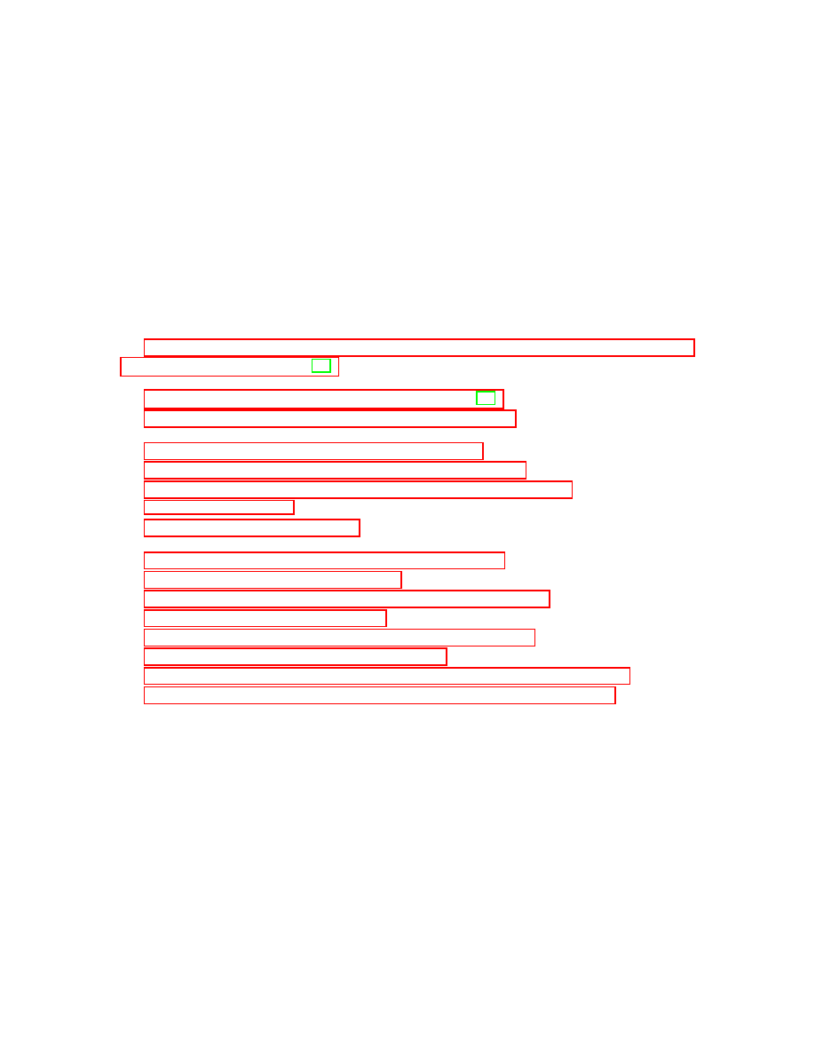
this hybrid model is shown in Figure 2.1. Hybrid detection is very effective because it
Figure 2.1: The hybrid model explanation for training phase and testing phase
from Masud et al. [27].
takes advantage of many types of features. But this mechanism is relatively complex
compared to the systems using traditional one-type feature extraction. The main
shortcoming is that several parameters have to be carefully tuned to control various
aspects of the system in order to achieve good results.
Like previous solutions, we use an n-gram sliding window as well. However, in or-
der to reduce the complexity of selecting the proper length for the n-gram, we shrink
its range by proposing a reasonable lower bound. Unlike Henchiri and Japkowicz
[17] using commercial anti-virus software, we construct families using clustering al-

Chapter 2: Related work
16
gorithms instead. Also one-class classification using only malicious code instead of
benign programs is implemented in this thesis. We will present more details about
these approaches in Chapter 4.

Chapter 3
Background
We believe similar malicious executables contain one or more common character-
istics. Since we cannot fully understand individual attacks at once, it is relatively
easier to retrieve key features from a group of similar malicious executable because
they share the same characteristics. Thus, analyzing malicious groups is strongly
required. In this circumstance, grouping malicious executables requires the knowl-
edge of clustering algorithms from data mining. It also demands some properties
from attacks in order to distinguish them. Therefore, techniques from information
retrieval are used to assign weights to malicious executables to differ similar or dis-
similar ones. Once we have the groups, alignment algorithms from bioinformatics
are applied to retrieve the common features that will be used to detect and identify
new attacks. In this chapter, we provide the discussion about malicious attacks in
Section 3.1, techniques from data mining, information retrieval and bioinformatics
are represented from Section 3.2 to Section 3.4. At last, performance measurement
is discussed in Section 3.5.
17

Chapter 3: Background
18
3.1
Malicious attacks
Generally, malicious attacks can be classified according to their functions and
their approaches to propagation. Based on these characteristics, Skoudis and Ziltser
[34] and McGraw and Morrisett [28] have categorized malicious attacks into the
following major types:
• Virus: A virus is a self-replicating program that depends on human interaction
such as opening malicious executables and reading e-mail. Once a virus is
accessed, it infects benign programs by attaching itself to them, or simply by
carrying out malicious acts. Computer viruses often have the ability to destroy
data on the hard drive, or even destroy hard drives.
• Worm: A worm is also a self-replicating program that can spread itself through
the network or through e-mail communication to other hosts. A worm does
not need a benign program to act as a host. Massive replication activity can
exhaust systems and network resources, leading to a crash. Well developed
networks for data sharing provide convenient environments for them.
• BackDoor: A backdoor is a hidden program in the computer system that
provides remote access that bypasses the normal authentication and security
checks. It usually does not self-replicate, spread or infect other files; however,
a backdoor program opens a tunnel for intruders to control the system, and
collect private information and sensitive data.
• Trojan horse: A trojan horse is another type of attack that does not self-
replicate. It arrives disguised as a legitimate program such as a screen-saver
or mini-game. A trojan horse usually does not self-replicate and infect other
clean files, but it actually executes unexpected and unauthorized operations.
Trojan horses are often used to steal sensitive information and destroy data.

Chapter 3: Background
19
• Spyware and Adware: Spyware collects user’ information such as online
activities and file access history. It usually hides itself within other programs.
Adware displays unwanted advertising. It can exhaust system resources and
cause the poor system performance.
This list only contains the major categories. Other types of malicious code such as
logic and time bomb and rootkit also exist. Since we are interested in Windows-
based malicious attacks, any executable using Intel X86 instruction set architecture
will be our target.
3.2
Clustering algorithms from data mining
Data mining or knowledge discovery is “a non-trivial extraction of implicit, previ-
ously unknown, and potentially useful information from data” [16]. It includes many
techniques such as frequent pattern mining, sequential pattern mining, clustering,
classification, outlier detection and so on. In this thesis, we are interested in group-
ing samples into classes without a priori knowledge of the resultant clusters. Hence
clustering algorithms fit perfectly in the solution framework of our problem.
Clustering is a technique that groups a set of data objects into clusters or classes.
Each cluster is a group of data objects that are similar to their cluster members
and dissimilar to objects from other clusters. In other words, clustering maximizes
the intra-cluster similarity and minimizes the inter-cluster similarity. In this case,
a distance function between any pair of data objects and a threshold defining the
meaning of closeness are required to construct the clusters containing similar data
objects. Clustering is also called unsupervised learning because clustering algorithms
do not require any dataset for the training purpose. Although many clustering al-
gorithms have been proposed, each of them demands a different set of parameters
to run. For example, the K-means [12], PAM [30] and CLARA [22] clustering algo-
rithms require the user to specify the expected number of result clusters. Algorithms

Chapter 3: Background
20
with this requirement are not adequate for our needs because we cannot specify the
number of result classes in advance.
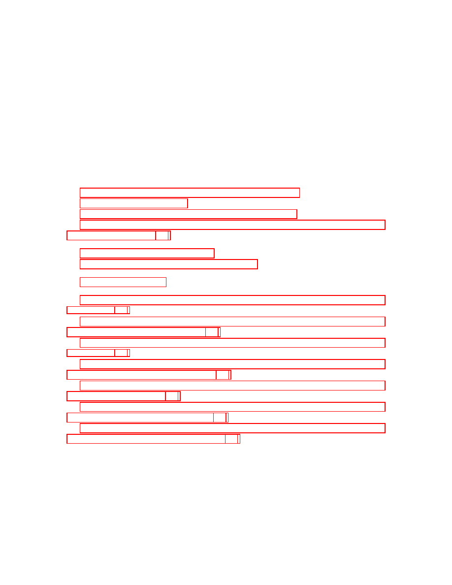
DBSCAN algorithm [13] on the other hand does not require the user to predefine
the number of result clusters as an input. It is based on the connectivity and density
functions to discover clusters with arbitrary shapes. There are two input parameters
for DBSCAN, the minimum number of points (MinPts) and a radius (Eps). This
algorithm relies on the following concepts (illustrated in Figure 3.1):
• Eps-neighborhood: number of neighbors within a radius Eps for a given
point.
• Core objects (CO): a set of points that each has at least MinPts points
within its Eps-neighborhood.
• Border objects (BO): a set of points that each has less than MinPts points
within its Eps-neighborhood.
• Directly density reachable (DDR):an point p is DDR from a CO q if p is
within an Eps-neighborhood of q.
• Density reachable (DR): a point p is DR from point q if there exists a chain
of DDR point from p to q.
• Density connected (DC): a point p is DC to point q if there exists a point
r such that p and q are DR from r.
In order to find clusters, DBSCAN arbitrarily picks a data object out of the
dataset. If the point is a border object, the algorithm just randomly picks other
points until it is a core point. If this object is a core object, the algorithm creates a
cluster with all its neighbors that are directly density reachable and further includes
the rest of the points that are either density reachable or density connected to any
point in this cluster. DBSCAN recursively repeats the same process until there is no
Chapter 3: Background
21
Figure 3.1: Terminology explanation from Ester et al. [13].
point that is neither density connected nor density reachable. Once this cluster is
built, the algorithm randomly selects the next un-clustered object, and repeats the
same procedure until there is no point left un-clustered in the dataset.
3.3
Techniques from information retrieval
Here, we use techniques from information retrieval which provide the ability to
determine the distances between data objects. In this section, we introduce the tools
from information retrieval: term frequency/inverse document frequency and cosine
similarity.
3.3.1
Term Frequency/Inverse Document Frequency
Term Frequency/Inverse Document Frequency (TF/IDF) is a measure of the
importance of terms within a document and across multiple documents [32]. In this
thesis, these terms are fixed-length sequences. There are two steps in calculating this
measurement. The first step is to calculate the occurrences of each individual term
(TF). However, some terms are very common, appearing in almost every assembly

Chapter 3: Background
22
code. Therefore, in the second step, IDF adds weights to balance the effects of
common terms. Given terms t
i
and documents d
j
, TF/IDF values of terms can be
calculated as follows:
tf idf
i,j
= tf
i,j
∗ idf
i,j
where
tf
i,j
=
n
i,j
P
k
n
k,j
and
idf
i,j
= ln
|D|
|{d
j
: t
i
∈ d
j
}|
where:
n
i,j
: number of appearances of the term t
i
in document d
j
.
P
k
n
k,j
: number of terms in document d
j
.
|D| : total number of documents.
|{d
j
: t
i
∈ d
j
}| : total number of documents in which term t
i
appears.
According to this formula, the TF/IDF value for any term is greater or equal to 0.
3.3.2
Cosine similarity
Cosine similarity is a tool to measure similarity using the angle between two
vectors. The elements of the vectors consist of a list of TF/IDF weights for each
term. Given two vectors X and Y , cosine similarity is defined as follows:
similarity(X, Y ) = cos(Θ) =
X · Y
|X||Y |
=
x
1
∗ y
1
+ x
2
∗ y
2
+ ... + x
n
∗ y
n
(x
2
1
+ x
2
1
+ ... + x
2
n
)
1/2
∗ (y
2
1
+ y
2
2
+ ... + y
2
n
)
1/2
where
X · Y : inner product of two vectors
Chapter 3: Background
23
|X| (|Y |) : the magnitude of vector X (Y )
x
i
(y
i
) : the TF/IDF weight for term t
i
in vector X (Y )
The value of cosine similarity originally is between 0 and -1. Since TF/IDF values
are the input and they are greater or equal to 0, the value of cosine similarity is
between 0 and 1. The closer the cosine similarity is to 1, the more similar the two
vectors are.
3.4
Alignment algorithms from bioinformatics
Bioinformatics is the discipline used to process information about the molecular
biology of organisms. Its objective is to analyze large amounts of data gathered from
genome sequences and other molecular diagnostics [5]. One of the bioinformatics
techniques is the sequence alignment. A sequence alignment is an approach of ar-
ranging the genetic sequences to identify similar regions that may be a consequence
of functional relationships between the sequences. From the result of clustering algo-
rithms, we have a set of clusters containing similar malicious executables. Therefore,
the multiple alignment is used first to extract the common characteristic in mem-
bers of each malicious family. Once we have this feature, the local alignment can
help to find unknown sequences that are locally or globally similar to these common
characteristics.
There are mainly two categories of sequence alignment, pairwise alignment and
multiple sequence alignment.
Both of them contain global and local alignment.
Pairwise global alignment [29] aligns all residues in one sequence globally with the
residues in another sequence; and pairwise local alignment [35] looks for identical
contiguous subsequence between two inputs. Let us consider an example. Given two
sequences X and Y in Figure 3.2 (a), the result of pairwise global alignment is in
(b), and the result of pairwise local alignment is in Figure 3.2 (c). In our project,
Chapter 3: Background
24
pairwise local alignment is used by applying features to detect new attacks. From
our assumption in Section 1.3.2, each malicious family contains at least one unique
subsequence of instructions that can represent the whole family. Once we retrieve
these instruction subsequences, any new attack holding such characteristics can be
detected and identified. Therefore, in order to measure the similarity regionally,
pairwise local alignment is the appropriate alignment technique.
Figure 3.2: Comparison between global and local alignments
Since pairwise local and global alignments only address the problem of aligning
two sequences at a time, what if we want to align multiple sequences to analyze their
similarities? This question leads us to the technique of multiple sequence alignment.
Multiple sequence alignment is an extension of pairwise alignment to globally or lo-
cal align more than two sequences at one time. There are many multiple alignment
algorithms, including progressive methods, iterative methods, alignments based on
locally conserved patterns, statistical and probabilistic methods and many others.
Here, we choose to use the CLUSTALW algorithm [37]. CLUSTALW is a greedy
method to globally align multiple sequences. First, it finds the two most similar
sequences and aligns them together. It then progressively adds less similar sequences
to adjust the result. CLUSTALW was originally designed to align a large number
of sequences that are close to each other. Since we first need to group the mali-

Chapter 3: Background
25
cious executables into classes before applying any multiple alignment algorithm, the
CLUSTALW algorithm becomes an excellent choice for our implementation. More
details about adopting multiple alignment to extract features can be found in Sec-
tion 4.3.
3.5
Performance measurement
In order to evaluate the performance of our system, we use the following mea-
surements:
• For detection:
1. True Positive (TP): number of malicious executables correctly classi-
fied.
2. True Negative (TN): number of benign executables correctly classified.
3. False Positive (FP): number of benign executables incorrectly classified
as malicious.
4. False Negative (FN): number of malicious executables mistakenly clas-
sified as benign.
• For identification:
1. True Identification (TI): number of malicious executables correctly
identified as members of their clustering family.
2. False Identification (FI): number of malicious executables not correctly
identified as members of their clustering family.
For the problems of detecting and identifying malicious executables, the secu-
rity system aims at accurately detecting both malicious and benign problems, and

Chapter 3: Background
26
correctly identifying malicious executables as well. Thus, we are interested in the
following quantities:
• Detection Rate (DR): number of malicious executables correctly detected
as malevolent regarding total number of malicious programs.
=
T P
T P + F N
• False Positive Rate (FPR): number of benign programs correctly detected
regarding total number of benign programs.
=
F P
T N + F P
• Overall Accuracy For Detection (OAD): the summation of both correctly
detected malicious and benign programs regarding the entire dataset.
=
T P + T N
T P + T N + F P + F N
• Identification Rate (IR): number of malicious executables correctly identi-
fied regarding total number of malicious programs.
=
T I
T I + F I

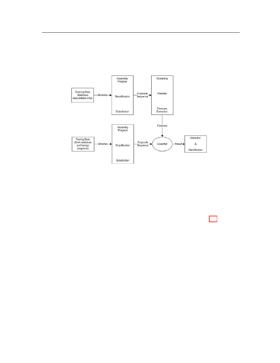
Chapter 4
Malicious code detection and
identification
In this chapter, we introduce the processes of our system: malicious data prepa-
ration in Section 4.1; clustering methodology in Section 4.2; feature extraction in
Section 4.3 and the application of features in Section 4.4.
4.1
Data preparation
The epidemiology of malicious executables is similar to biological malicious dis-
eases and viruses because of their ways to propagate, break out and self-replicate. In
biology, diseases and viruses are simple organisms whose functionalities are mainly
controlled by their genome sequences. Our first challenge is to find genome-like
representations for malicious executables. As we stated previously, we assume pro-
grammers try to change opcodes or operands to bypass signature detection, but they
cannot change the instruction sequences too much in order to keep similar functional-
ities. Each instruction is composed of an opcode and some operands, and the opcode
primarily determines the intention of an instruction. In this case, the opcode is the
27

Chapter 4: Malicious code detection and identification
28
core component of each instruction. Therefore, opcodes could be considered as the
“nucleotides” within destructive attacks. In this section, we present our approach for
transforming malicious executables from binary formats into their simulated “pro-
tein” sequences, which we call s-opcode sequences.
4.1.1
Disassembly
We know that malicious executables are programs represented in binary formats.
Since we only examine the executables using 32-bit Intel
R
Instruction Set Architec-
ture [21], binary executables can be translated into low-level assembly language to
extract instruction sequences using a disassembler. In our project, we use a free tool,
IDA disassembler [9], to decode malicious attacks. After disassembling them, each
attack becomes a file containing thousands of lines of decoded instructions and their
corresponding positions in binary files. The only data we need from each instruction
is its opcode. By ignoring parameters and other disassembled information, the as-
sembly code of each binary executable is simplified into a sequence of opcodes. Let
us consider an example of the transformation from a binary sequence to its s-opcode
sequence (see Figure 4.1). Given the binary sequence, “B430 CD21 86E0 3D1E 03BE
B407 730A BEA5 103C 0A74 03BE C91E”, this disassembly phase is shown in steps
one and two of the figure.
4.1.2
Opcode grouping
A malicious executable can be seen as a sequence of opcodes. However, there
are about two hundred opcodes within the Intel
R
instruction set [21]. It is easy for
programmers of malicious executables to obfuscate attacks. For example, a for-loop
with increment can be changed to a while-loop or for-loop with decrement or many
other implementations. But no matter how they change, a loop has to include the
arithmetic and control instructions. Under this circumstance, we try to categorize
Chapter 4: Malicious code detection and identification
29
Figure 4.1: Binary to s-opcode sequence transformation
hundreds of opcodes into a relatively small number of groups whose opcodes have
similar functionality. According to the guideline from Intel [21], the company has
already classified its opcodes into thirteen categories. Because of the duplication of
these categories, we further simplify the Intel grouping into eleven categories. More
details about opcode grouping can be found in Appendix A. Just as genome sequences
use a single character to denote each amino acid, our categories in Table 4.1 are also
represented with unique single characters.
4.1.3
s-opcode sequence transformation
Each opcode in an opcode sequence is substituted by a single character according
to the opcode grouping specified in Table 4.1. After opcode substitution, an opcode
sequence is turned into the corresponding s-opcode sequence with single-character
opcodes. In biology, both DNA and RNA sequences have four types of nucleotides
and protein sequences are composed of twenty types of amino acids [5]. Since we
group Intel opcodes into eleven groups, s-opcode sequences fit nicely into the domain

Chapter 4: Malicious code detection and identification
30
Intel instruction Category
Character representation
Data Transfer Instructions
D
Arithmetic Instructions
A
Logical Instructions
L
Shift and Rotate Instructions
T
Bit and Byte Instructions
H
Control Transfer Instructions
C
String Instructions
S
I/O Instructions
I
Flag Control Instructions
F
Segment Register Instructions
R
Miscellaneous Instructions
M
Table 4.1: Single character representation of opcode categories.
of bioinformatics algorithms. Now, we can treat s-opcode sequences as biological
genome sequences, and apply bioinformatics techniques such as the alignment algo-
rithms described in Section 3.4 to address the problem of detecting and identifying
malicious executables. This transformation phase is shown in step three of Figure 4.1.
4.2
Clustering
There are at least two ways to detect new attacks. The first approach is to find the
key features from the existing malicious executables, then use these characteristics to
recognize new malicious executables. The second approach is to construct malicious
families based on the properties of attacks. Using these families, we can extract
features from each family to discover new attacks. Between these two approaches,
the first one is more like an idealistic method. It is very complex to find the crucial
information directly from attacks. The second approach on the other hand is more
practical. Malicious families can be formed based on their properties, for example
s-opcode sequences, and it is easier to retrieve key data from members in the same

Chapter 4: Malicious code detection and identification
31
family since they share similar characteristics. In contrast with malicious families, a
single executable alone provides insufficient information to find its characteristics. In
our project, we apply the second method to extract features from clustered malicious
families.
After the transformation from binary code to s-opcode sequences, our task now
is to find a way to cluster malicious attacks algorithmically. In commercial industry,
security software programs have their own approaches to classify malicious executa-
bles. A new malicious attack is analyzed for its functionalities, propagation and many
other characteristics by experienced analysts. Then, these newly reported attacks
are manually classified into families. In this case, human beings play an important
role in forming the groups of malicious executables. For the same reason, different
companies have different understandings of attacks, and therefore, have slightly dif-
ferent identification results for existing malicious executables. In order to construct
malicious families algorithmically, clustering algorithms from data mining can be
used to address the problem of grouping.
In clustering algorithms, there are two important components, a distance function
and a distance threshold. The distance function is also called the distance measure-
ment or similarity measurement and quantifies the difference between any pair of
data objects. The distance threshold is a constraint that determines whether two
data objects are close enough or not. In this thesis, we use a combination of cosine
similarity and TF/IDF to measure the difference. Heuristic approaches introduced
with the DBSCAN algorithm help choosing the distance threshold.
4.2.1
Distance measurement
Given a s-opcode sequence with a length of n, we choose a fixed window length
k where k ≤ n. By sliding the length k window through the s-opcode sequence, we
obtain a vector containing (n − k + 1) subsequences where each subsequence is a term
Chapter 4: Malicious code detection and identification
32
with k-opcodes. An example is shown in Figure 4.2 with sliding window of length 8.
The s-opcode sequence with length 13 can be decomposed into 6 subsequences with
length 8. Using this vector representation, each vector has a list of subsequences
which have length k. The TF/IDF value for each subsequence is calculated over all
the available subsequences. After calculating the value for TF/IDF, each vector has
a list of terms associated with their TF/IDF values. Every malicious executable is
now represented in vector space as pairs of k-length subsequences and their TF/IDF
values.
Many distance functions such as Euclidean distance, Manhattan distance and
Jaro distance [14] have been developed to measure the differences between two data
objets of their coordinates in metric space. In our project, instead of measuring geo-
metrical distances between two vectors, we are interested in estimating the direction
and angle of them. The direction and angle between two vectors provides precise
information about how they differ in functionalities that are instruction sequences
in our case. This is the reason that cosine similarity is chosen to measure the angle
between two vectors. Our next step is to apply the vector representations to the
cosine measurement.
Figure 4.2: Sliding window used to retrieve length k term list.
Applying the formula of cosine similarity described in Section 3.3.2, the distance
between vectors A and B can be found in a numeric range of 0 to 1. By collecting all
results of cosine similarity, a score matrix can be generated to represent the distance
Chapter 4: Malicious code detection and identification
33
between any pair of vectors in the dataset. In cosine similarity, the closer to value 1
the distance is, the more similar the two vectors are. In order to follow the meaning
of distance in a natural way, we subtract all the elements in the score matrix from
1. After this adjustment, the adjusted score matrix in Table 4.2 as an example gives
an opposite meaning to the cosine value. The value 0 means that two vectors are
identical. The closer to the value 0 the score is, the more similar the two vectors
are. For example, object “NB-P.COM” is more similar to object “NB-O.COM” than
object “A 204.COM” because the score between object “NB-O.COM” and object
“NB-P.COM” is smaller.
A 204.COM
NB-O.COM
NB-P.COM
NB-T.COM
NB-U.COM
A 204.COM
0
NB-O.COM
0.9904101
0
NB-P.COM
0.9919908
0.1834956
0
NB-T.COM
0.990327
0.1748854
0.0487555
0
NB-U.COM
0.9903327
0.1708549
0.0556605
0.046651
0
Table 4.2: Adjusted score matrix.
4.2.2
Clustering algorithm
Once we have the distance matrix for all data objects, the next challenge is to
choose a proper clustering algorithm. We use the implementation of hierarchical
clustering from R [40] with the input of a TF/IDF-Cosine distance matrix to find
the potential number of result groups of our dataset and the possible threshold to
determine the neighborhood. The result from hierarchical clustering is shown in
Figure 4.3. The height at value 0 according to cosine similarity is for objects that
have exactly the same angle (identical). At this distance, every malicious executable
forms a cluster for itself. When we increase the distance from a value of 0 to around
0.1, several clusters are built by merging similar attacks. As the distance further
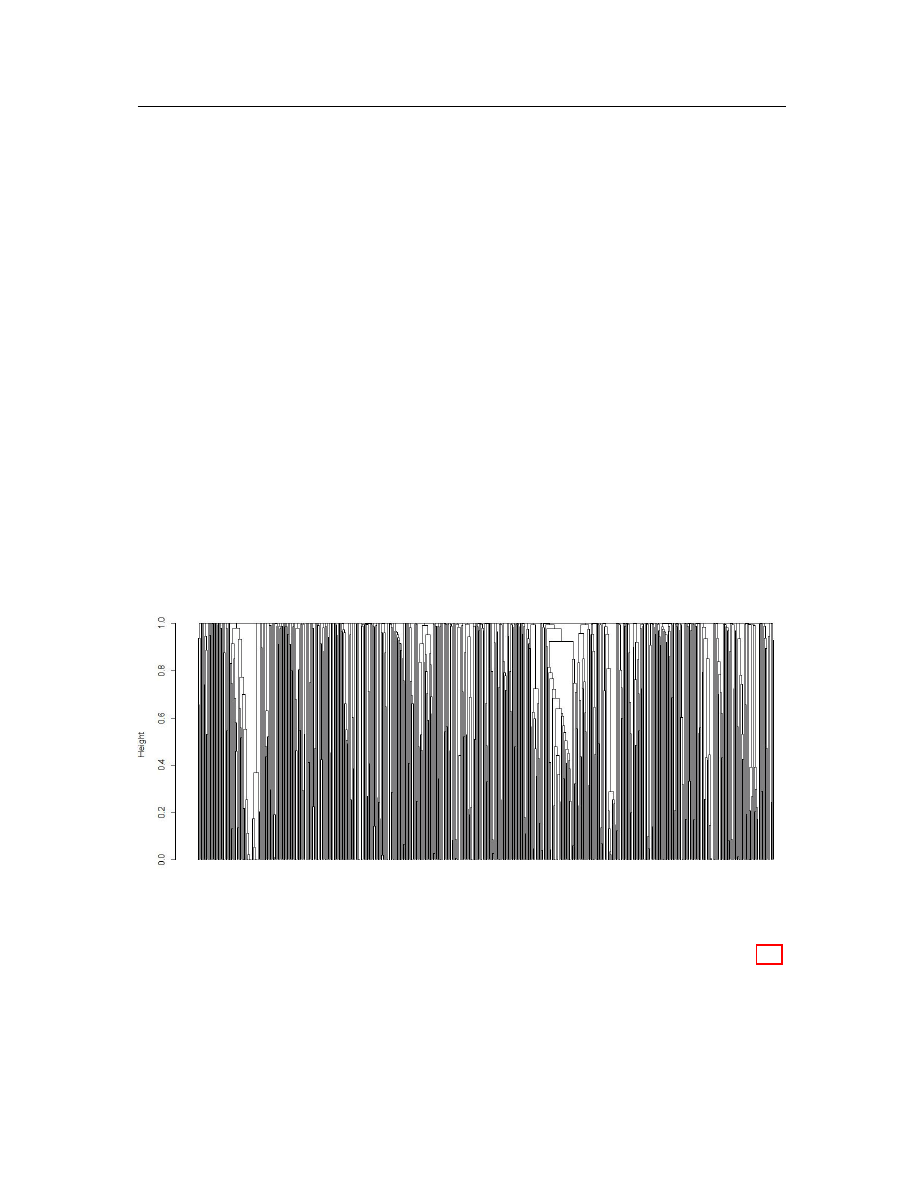
Chapter 4: Malicious code detection and identification
34
increases, some lines merge together into bigger classes. Fewer and fewer classes can
be formed as the distance approaches 1. A relatively small number of clusters is
constructed overall because we randomly select training samples from the dataset.
The graph shows that similarities between malicious executables within the same
cluster are lower than the similarities between malicious executables from different
families. If we can choose a proper threshold, the clustering algorithm is capable of
constructing some clusters from malicious samples based on their TF/IDF-Cosine
similarity. However, from the result of the hierarchical clustering algorithm, there
is no way in advance to predict the possible number of result classes given the fixed
threshold. All similar malicious executables should be able to be grouped into the
same class without predefined clusters. Because of this constraint, there are only a
few clustering algorithms such as nearest neighbor and DBSCAN algorithms that we
can choose. By testing these clustering algorithms, we find that DBSCAN generates
the categorization that is the closest to the result from commercial anti-malware
products.
Figure 4.3: Result from a complete hierarchical clustering algorithm.
DBSCAN is a density-based algorithm. We introduced DBSCAN in Section 3.2

Chapter 4: Malicious code detection and identification
35
along with its two main parameters. The first parameter is the minimum number
of points within the neighborhood. In our domain, no attack is considered noise.
Therefore, minPts can be set to 1. This allows the smallest family to have at least
two members (a core object and a neighbor). The attack without neighbors builds
a cluster only with itself. The second parameter is the radius used to form the
neighborhood. From the result of the hierarchical clustering algorithm in Figure 4.3,
there are clusters existing in the range of approximately 0.4 to 0.8. Thus, the radius
can be chosen within this range. A detailed heuristic method to choose the DBSCAN
radius is presented in Section 5.3.1.
4.3
Feature extraction
After applying the clustering algorithm, malicious executables are grouped into
different families containing similar attacks. The next obstacle is how to retrieve the
feature from each family. But first of all, what is a “feature” in our domain? As we
stated in Section 1.3, there exists at least one common subsequence of instructions
that is similar or identical among all malicious members from the same family. This
common subsequence is relatively different from other attacks because different fam-
ilies contain comparatively different s-opcode sequences. In this case, these unique
instruction sequences from malicious families become our features. Now we under-
stand the domain of our features, but how can we find specific features? When we
prepared the data objects, we translated the instruction sequences into genome-like
s-opcode sequences. Then all the s-opcode sequences in each class can be aligned
according to their best local sequences using the multiple alignment algorithm de-
scribed in Section 3.4. By searching through the output of multiple alignment, we
can extract the most common s-opcode subsequences as features. In other words, fea-
tures are the local subsequences from each class that appear in every member of that
cluster. The example in Table 4.3 shows a malicious family with two common subse-

Chapter 4: Malicious code detection and identification
36
quences. In the table, the subsequences DSDDCDCDDARDDSDDDDDDD and
ADADDADD are the common s-opcode sequences that could be features.
NB-P.COM
DSDDCDCDDARDDSDDDDDDDSAHADADDADD
NB-T.COM
DSDDCDCDDARDDSDDDDDDDDDDADADDADD
NB-U.COM
DSDDCDCDDARDDSDDDDDDDSDHADADDADD
NB-O.COM
DSDDCDCDDARDDSDDDDDDDDDMADADDADD
Table 4.3: Multiple alignment that has common subsequences.
Common subsequences generated from multiple alignment can have various lengths
from family to family. We have found that their lengths vary from 1 to 20 or even
more. The question is how to gather the important features. There are many options
here. The first choice is that we can define a threshold according to the length of the
sliding window. Any common subsequence with length greater than this threshold
can be selected as the feature. The rest are considered to be insignificant. A second
choice is that we ignore the threshold, but choose the longest or the top two longest
common subsequences as features. We have decided to use the subsequences that are
the longest or the two longest common subsequences whose length is greater than
the length of the sliding window as features.
Using common subsequences as the feature suggests a matching threshold with
value 100%. It means that all members in the family have to carry a or some specific
subsequence(s). Unfortunately, some clusters do not have any common subsequence
at all or the length of the common subsequences is not long enough. For these
special clusters, we can reduce the value of the threshold to retrieve proper features
other than common subsequences. But how do we choose the proper value? Should
it be 70%, 80% or 90%? In this circumstance, we introduce a simple approach to
determine the value of the threshold. If we choose the length of the sliding window to
be a fixed value n in the process of data preparation, then the length of the features
should also be greater than n. While the threshold is changing, we can examine the
Chapter 4: Malicious code detection and identification
37
changes of the size and the content of the resulting subsequences to choose a proper
value for the threshold.
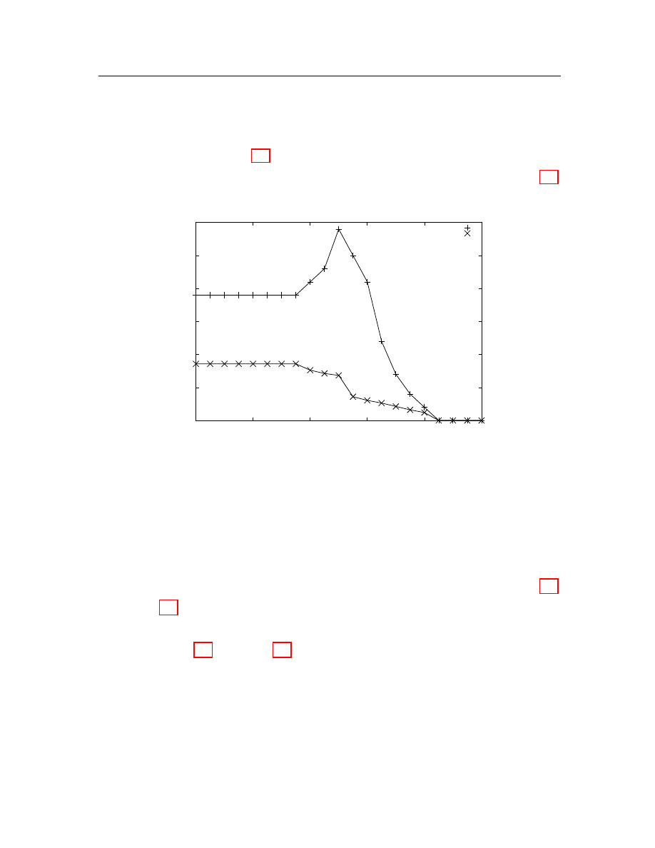
For illustration, Figure 4.4 shows how the size of the feature list changes by
varying the threshold for a cluster without any common subsequence. Tables 4.4
lists changes of the content of the feature list.
0
5
10
15
20
25
30
0
0.2
0.4
0.6
0.8
1
Size
Threshold
A
B
C
the size of features list
average length of features
Figure 4.4: Feature list size.
While we are altering the threshold from 5% to 100% with 5% granularity, both
the content and the size of the result list change. The size of the list is first flat
on a fixed value, then increases to a peak value and at last goes down to the value
zero as the threshold approaches 100%. Let us examine the contents as well. As the
size of the subsequence list approaches the peak value (point B in both Figure 4.4
and Table 4.4), the average length of subsequences decreases. But, some of the
subsequences are still long enough to be features. Once the size starts dropping (point
C in both Figure 4.4 and Table 4.4), subsequences become shorter and irrelevant to
the problem of detecting and identifying malicious attacks. Therefore, we select a
value on the up-slope curve as the threshold. Then, the longest sequences are picked

Chapter 4: Malicious code detection and identification
38
Point A
Point B
Point C
D
D
C
CD
C
D
DS
CD
S
CDD
DS
DC
DDMD
DD
DD
AAACCD
CDD
DS
CDCCDD
CDC
AD
SSDDMC
CDMD
AA
CACDMCC
DACD
CD
DDDDDDM
DDMD
DCD
MDMDDDD
LDCA
DDD
LDCACDACD
MDDDM
CDD
CDMDSMDDDM
AAACCD
CCD
CDDDMDLDCDMD
SSDDMC
DACD
DDAMMSMDDAADD
CACDMCC
MDDD
ACDAACCACDDDCD
MDMDDDD
DDCC
DDCCLCDCDDMDCD
DDDDDDM
DDMD
AADDTTFADLDDDDDC
ACDAACCACD
DDMC
RDDRDDDDTDRDDDAADADDDDDD
CDDDMDLDCDMD
DDDA
DDAMMSMDDAADD
CDMCC
DDCCLCDCDDMDCD
DAACC
AADDTTFADLDDDDDC
DADDDD
RDDRDDDDTDRDDDAADADDDDDD
CDDDMD
MDMDDDD
DDAMMSMDDA
Table 4.4: The content of the feature list changes by varying the threshold referring
to Figure 4.4.
as features according to the selected threshold. Since the threshold is arbitrarily
chosen in a range, the result of the feature list is slightly different at each time of
extracting features. By applying this approach, the priority of the feature extraction
is to find common subsequences as features. Then, for those clusters without any
common subsequence, the secondary goal is to find the feature that satisfies the
chosen matching threshold.

Chapter 4: Malicious code detection and identification
39
4.4
Applying features to the problems of detec-
tion and identification
After clustering and feature extraction, we have a set of families of known ma-
licious executables and a list of s-opcode sequences as features that can represent
the characteristics of these malicious families. The next step is to apply features to
detect and identify attacks. For any incoming attack, we use the same transforma-
tion processes: disassembling it into a sequence of instructions; retrieving its opcode
sequence and translating it into an s-opcode sequence. Then, a bioinformatics-based
classifier using s-opcode sequences is applied to perform the tasks of detection and
identification.
Given a set of features and their families, our challenge is to apply the advantages
of bioinformatics analysis. According to our hypothesis, each malicious family has
at least one key subsequence that is unique compared to other families.
If any
subsequence from a program is similar or identical to the features appearing in our
database, then this executable can be flagged as a malicious program. The question is
how we are going to compare them. This question requires the knowledge of the local
alignment algorithm. We have described the local alignment in Section 3.4. Pair-wise
local alignment is used to find the similar subsequences in both inputs. Therefore,
for any possible incoming executable, we locally align its decoded s-opcode sequence
with all the features in our database. In order to tell whether two sequences are
close enough or not, we introduce a similarity threshold to distinguish them. This
threshold can vary from 0% to 100%. If the value of the threshold is 100%, then the
local alignment is a scheme with exact matching. On the other hand, decreasing this
threshold gives a better tolerance of detecting new attacks with mutated s-opcode
sequences. However, the threshold cannot be too low. Too low a threshold will
generate a large number of false alerts. We will investigate this in Chapter 5.
In addition to the detection, if there is a match between an incoming attack and
Chapter 4: Malicious code detection and identification
40
the feature in the database, we can retrieve its most similar feature(s). By using these
features and the families where they appear, we can signal the families to which the
attack belongs.
Figure 4.5: Processes of our approach
4.5
Summary
In summary, the procedures of our approach are outlined in Figure 4.5. First of
all, malicious samples are randomly selected from the dataset, and we apply the pro-
cesses of decoding, simplifying and substituting to obtain their s-opcode sequences.
Features extracted from clustered malicious families are then used by the classifier.
The classifier uses these features to achieve the goal of detecting and identifying new
incoming attacks.

Chapter 5
Experiments and Performance
Evaluation
The features we extract from binary executables can be applied at either the
application level or the networking level. This chapter presents results for our ap-
proach in detecting and identifying attacks at the network layer in simulated network
traffic. As we will see in Section 5.3, we try to optimize system parameters in order
to achieve the highest accuracy. Shortcomings that affect the results are analyzed
afterwards, and possible alternative solutions are also presented.
5.1
Datasets
We have a dataset containing 3548 malicious executables and 200 benign files.
The malicious executables were gathered from VX Heavens [1], and the benign pro-
grams come from the Windows XP operating system. The malicious executables
consist of a large number of DOS viruses, Windows malicious EXE or application
programs and a small number of trojan horses. The malicious attacks and benign
files were disassembled and then stored for the purposes of either training or testing.
41

Chapter 5: Experiments and Performance Evaluation
42
We input one fifth of the set of malicious executables into the training phase. After
their features are extracted, both malicious and benign files are used to test the
performance of this system.
If we could deploy our system in the field, then we would use all attacks from our
dataset for training purposes to predict unknown threats online. However, in order
to evaluate our technique, the dataset is divided into two sets, a training set and a
testing set. The idea is to mimic the current knowledge with the training set and
have the testing set serve as the new and unknown threats. Thus we can estimate
how effective our technique would be in realistic settings. Having a relatively small
training set would put an unfair stress on the system since it is unreasonable to
expect that one could learn anything effectively from a small sample. Having the
training set too large , on the other hand, would also be unfair because it would be
strongly biased towards our proposal. We have thus decided to use only 20% of our
dataset as the training set. As we shall see this is enough for us to deliver very good
performance, but also offers a scenario to illustrate how well the technique might
perform when one knows much less about the real set of threats that exist.
5.2
Experiment setup and simulation
All implementations were developed in Java with JDK 1.6. We used an external
Java package, Similarity Measurement Library [7], which implements the local align-
ment algorithm [35] to measure the similarity between two s-opcode sequences. In
addition, a Java version of CLUSTALW [19] was used for aligning malicious s-opcode
sequences in the same cluster.
For our simulations, we simulated a device in the network layer of the Internet.
In this layer, communication data is organized in the form of a series of TCP/IP
segments. The payload of a TCP segment is assumed to be 1400 bytes, and the
average length of an instruction is assumed to be four bytes. Therefore, each seg-

Chapter 5: Experiments and Performance Evaluation
43
ment contains approximately 1400/4=350 instructions with 350 opcodes. In order to
simulate the network traffic, we break each malicious s-opcode sequence into several
subsequences, each with a length of 350 or less if the length of the s-opcode sequence
is not divisible by 350. A classifier is deployed in the simulated device to examine
each incoming segment to determine whether its contents are malicious. If one or
more segments from a session are identified as malicious, then the whole session is
blocked.
5.3
Results
First, we randomly selected 710 malicious executables (20% of the dataset) as the
training set. After their transformation, DBSCAN was applied to this training set
by using the measurements of TF/TDF and cosine similarity. As a result, roughly
300 clusters were built. These clusters contain an unbalanced number of members
that are relatively similar to each other; we call each cluster a malicious family. By
assumption, similar malicious executables contain one or a few opcode subsequences
that are unique compared to other attacks. These key opcode subsequences can be
gathered by using multiple alignment among the members in each family. We used
the CLUSTALW algorithm to extract features (the most common subsequences)
from each family. After extracting the subsequences, there are approximately 300
features. The classifier then applies the local alignment technique to detect and
identify unknown malicious attacks using these features.
The procedures described above depend on various parameters. Next, we intro-
duce these parameters and possible ways for selecting their values.
5.3.1
Parameter selection
There are four parameters in our approach:

Chapter 5: Experiments and Performance Evaluation
44
1. The length of the n-gram for sliding through the s-opcode sequence.
2. The minimum number of points within the neighborhood, needed by DBSCAN.
3. The radius used to build the neighborhood, needed by DBSCAN.
4. The threshold for local alignment similarity used to measure the distance be-
tween two s-opcode sequences.
The length of the n-gram can take values from 1 to the length of the maximum
s-opcode sequence, but we are interested in the size of basic blocks in assembly codes.
A basic block is defined as “a sequence of consecutive statements (instructions) in
which the flow of control enters at the beginning and leaves at the end” [3]. Previous
analysis shows the size of basic blocks from SPEC benchmark programs varies roughly
from 5 to 15 instructions [20].
For example, blocks such as if-else and for-loop
statements require at least 4 to 5 instructions. In order to perform some extra
functions besides basic control statements, we assume a meaningful malicious block
has to be over 8 instructions long. Our experiments test the basic blocks starting at
length 8. Also, the minimum s-opcode length of an important feature corresponds
to the length of the n-gram.
The minimum number of points in the neighborhood and the neighborhood radius
are required parameters for DBSCAN. According to Ester et al., the radius to build
the neighborhood can be found approximately using a graphical representation [13].
We calculate the average distance for each data object to its k nearest neighbors.
After sorting the distances among all points, we can plot the sorted values in a graph,
which will have a “valley” shape. We select the value of the radius somewhere around
the valley. In this thesis, we follow this process by varying k values from 2 to 16.
Figure 5.1(a) shows the “valley” shapes with a broken or shifted line around value
from 0.5 to 0.7. If we zoom in the graph using distances from 0.3 to 0.8, we obtain
more details about this area (see Figure 5.1(b)). The “valley” representing the sorted
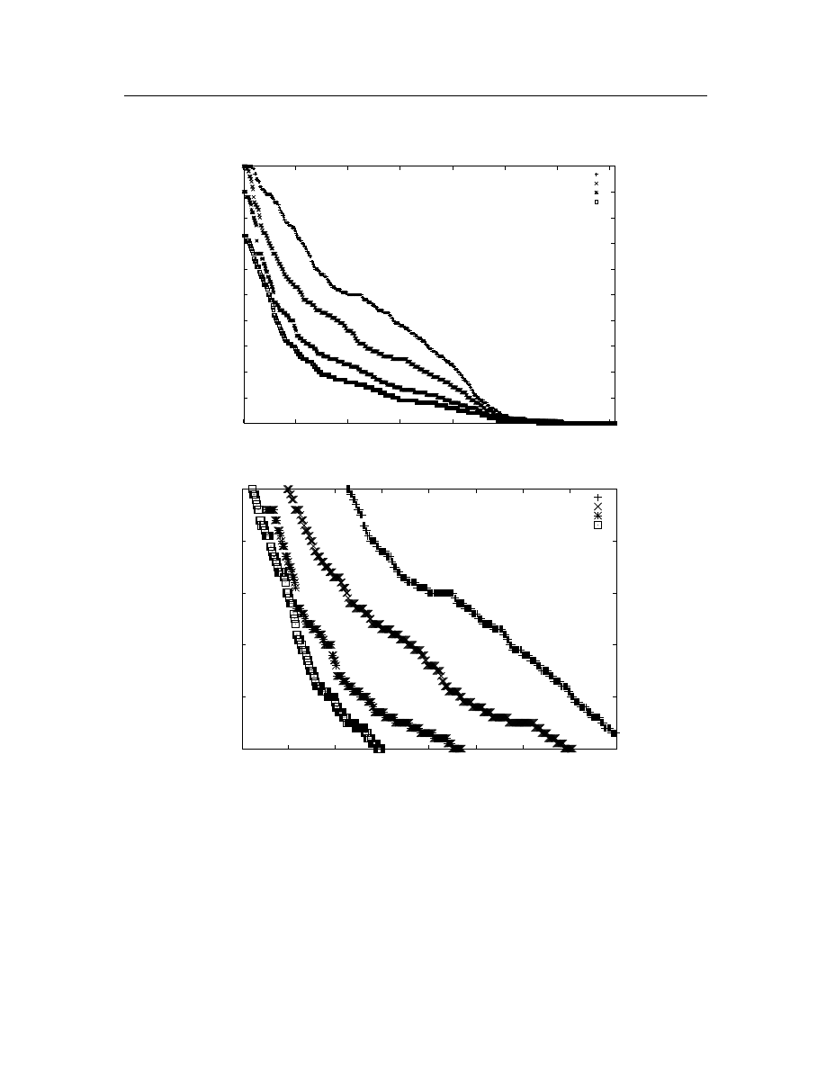
Chapter 5: Experiments and Performance Evaluation
45
0
0.1
0.2
0.3
0.4
0.5
0.6
0.7
0.8
0.9
1
0
100
200
300
400
500
600
700
Distances to its n nearest neighbors
Data points (unit)
K = 2
K = 4
K = 8
K = 16
(a) Sorted average distance to k nearest neighbors.
0.3
0.4
0.5
0.6
0.7
0.8
50
100
150
200
250
300
350
400
Distances to its n nearest neighbors
Data points (unit)
K = 2
K = 4
K = 8
K = 16
(b) Enlarged area for distance from 0.3 to 0.8.
Figure 5.1: Sorted average distance to k nearest neighbors.

Chapter 5: Experiments and Performance Evaluation
46
average distance to two nearest neighbors shifts approximately at value 0.5, and the
sorted average distance to eight nearest neighbors breaks roughly at value 0.65.
Values around where the “valley” is shifted or broken can be selected as the
radius to create the neighborhood with the specified number of neighbors. From
Figure 5.1, the radii match the result from our hierarchical clustering analysis in
Section 4.2.2 that malicious families exist in a range of approximately 0.4 to 0.8.
Using this approach, we can determine the value of the radius to create the proper
neighborhood. For determining the minimum number of points, we have to consider
the problem of detecting malicious executables. In clustering malicious attacks, there
is no noise. Malicious executables with neighbors create families to include them,
and the rest of the attacks without any neighbors build singleton families.
The last parameter is the threshold measuring the local alignment similarity. Its
value varies from 0 to 1. If the value is 1, then the local alignment is an exact match.
Otherwise, we are loosening the constraints of the local alignment.
In summary, the two parameters we have to address are the length of the n-gram
and the threshold measuring the local alignment similarity. Hence, we focus on the
performance of the system using various combinations of these two parameters.
5.3.2
Analysis
Since we have narrowed the system parameters down to two, we first run exper-
iments against the training set. These are divided into two parts. First, we fix the
threshold of local alignment similarity and test the system by varying the n-gram
length. Next, we use the n-gram length from the first part which achieves the highest
accuracy, and change the value of the local alignment threshold.
5.3.2.1
Experiments against the training set
n-gram length

Chapter 5: Experiments and Performance Evaluation
47
Threshold
n-gram Length
10
14
18
22
0.6
0.57
0.578
0.577
0.621
0.8
0.578
0.627
0.922
0.929
1
0.749
0.916
0.921
0.9175
Table 5.1: Overall accuracy of detection.
Single segment examination
In this test, we first need to select a value for
the local alignment threshold. But, how do we choose a proper value? As we know,
this threshold should not be too low because a low threshold will cause false alarms.
A local alignment threshold of 0.6 is a reasonable lower bound. However, in order
to select a proper value within this range, we have to further understand macro
behaviors of our system using both the local alignment threshold and the n-gram
length as parameters. Applying individual segment examination, Table 5.1 provides
a high-level view of changes of overall accuracy of detection (OAD) using various
combination of both parameters. In the table, the highest OAD values appear when
the threshold is at 0.8. Therefore, we select the threshold to be 80%.
As we discussed in previous sections, a basic instruction block is assumed to be
at least 8 instructions long. Therefore, our experiments start with an 8-gram length.
After running the clustering algorithm using the information provided from the n-
gram length, we extract from each family the most common longest subsequences,
as features, whose length is greater than n. In this case, each family only contributes
one feature to represent its characteristics. We assume the classifier resides in a net-
work device and examines each individual segment. Before we examine any segment,
we choose the threshold to be 0.8 to define the meaning of similarity. If there is a
match between a disassembled payload and a feature from our database with a simi-
larity over this threshold, the classifier will report the segment and block the session.
In this scenario, the classifier only examines one segment at a time, and reports
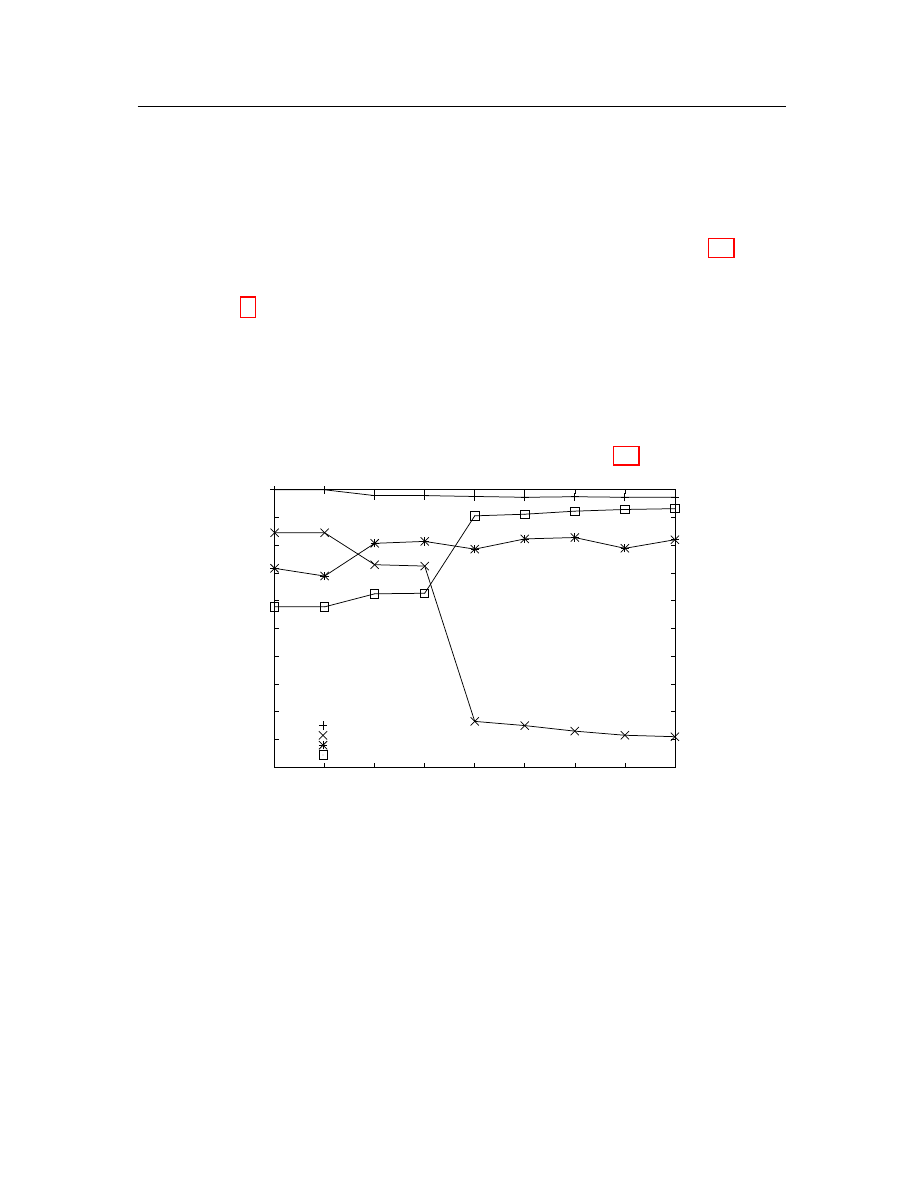
Chapter 5: Experiments and Performance Evaluation
48
the alert as soon as it identifies the examined segment as malicious. The classifier
does not require any memory to store the information about blocked sessions. We
call this approach the individual segment examination. Results for the individual
segment examination using different n-gram length are shown in Figure 5.2. The
corresponding numeric data of this graph and the following graphs can be found
in Appendix B. In this and the next graphs, Detection Rate (DR) is the fraction
of malicious executables correctly detected. False Positive Rate (FPR) is the frac-
tion of benign files mistakenly detected as malicious. Identification Rate (IR) is the
fraction of malicious executables correctly predicted from their own families, and
Overall Accuracy of Detection (OAD) is the overall accuracy of both detection and
false positive rates. These definitions can be found in Section 3.5.
1
0.9
0.8
0.7
0.6
0.5
0.4
0.3
0.2
0.1
0
24
22
20
18
16
14
12
10
8
Rate
Length of the N-gram
DR
FPR
IR
OAD
Figure 5.2: Individual segment examination
The graph shows detection rates of over 97%. Individual segment examination
gives a good detection rate because once there is a match in any one of the segments,
the session will be reported and blocked. However, the false positive rate is relatively
high. This is because of the noise feature. When the length of the n-gram is small,

Chapter 5: Experiments and Performance Evaluation
49
there are many s-opcode sequences in the feature list that commonly appear in the
assembly code. Benign programs containing these common s-opcode sequences are
also reported. Therefore, both detection and false positive rates are affected by
false alarms. Actually, as we increase the length of n-gram, the false positive rate
drops quickly. However, its value is still above 10%. For example, with the 18-
grams sliding window, even though we have a detection rate above 95%, the false
positive rate is roughly 17%. In contrast to the detection rate, the identification rate
increases as the length of the n-gram increases because the longer n-gram becomes
more characteristic and provides more information about targets. We want to select
the n-gram length which can achieve both the highest OAD and IR. In this case, our
experiments suggest that an n-gram length above 18 provides the highest accuracy
for individual segment examination.
The main drawback of checking a individual segment is the relatively high false
positive rate. Our next job is to reduce false positives while maintaining the same
detection rate. There are two options to ameliorate the current situation: improving
the quality of features or introducing more features.
Single segment examination using merged features
In the previous ex-
periments using features to examine individual segment, we get high detection and
false positive rates because of the noise feature. To remove noise from features, we
can merge similar features. When a feature is extracted from a family, a scanner will
search the feature list for either its super-sequences or subsequences or features that
are similar enough in other similarity measurements, for example local alignment [35],
Euclidean distance [14] and so on. If the scanner finds a super-sequence feature,
the newly generated feature will be dropped. If the scanner observes sub-sequence
features, the current feature will be included in the feature list by eliminating its
children. Otherwise, if similar features are found, only the longest one among them
is kept. By merging the features, approximately 20% to 30% of the original features
Chapter 5: Experiments and Performance Evaluation
50
are pruned out.
1
0.9
0.8
0.7
0.6
0.5
0.4
0.3
0.2
0.1
0
24
22
20
18
16
14
12
10
8
Rate
Length of the N-gram
DR
FPR
IR
OAD
Figure 5.3: Individual segment examination with merged features
Figure 5.3 shows the experimental results for the merged features generated from
different n-gram length. The detection rate is sacrificed a little as a compromise for
the drop of the false positive rate for merged features compared to original features.
For example, using the 18-grams, the false positive rate drops by roughly 1% to
12% while the detection rate is maintained at 93%. However the false positive rate
is still above 10%. After merging the feature list, the effect of noise features has
been reduced. The high false positive rate now could be due to the organization
of executables. The assembly code consists of both execution and data segments.
Lots of data segments or “NOP” operations mix with executable instructions. In
our simulation, we have to remove all unrelated segments to retrieve s-opcode se-
quences. This removal causes s-opcode sequences from some segments to be shorter
and non-characteristic.
These non-characteristic s-opcode sequences trigger false
alarms. Therefore, merging similar features does not improve accuracy very much.
In our experiments, the identification rate drops quickly because merging features

Chapter 5: Experiments and Performance Evaluation
51
causes the loss of information about the families they belong to. Eventually, this
leads to a lower identification rate. Interestingly, false positive rates from 10-grams
and 12-grams drop significantly compared to the rate from 14-grams. This is because
short noise features from both 10-grams and 12-grams are comparatively easier to
merge. The more noise features are merged, the better the quality of the feature
list. The graph shows that the n-gram with a length above 18 provides the highest
accuracy.
Threshold
n-gram Length
10
14
18
22
0.6
0.613
0.618
0.621
0.646
0.8
0.63
0.745
0.945
0.951
1
0.8105
0.927
0.93
0.909
Table 5.2: OAD using double segments examination
Double segments examination
The last two sets of experiments show that
the false positive rate generated from examining individual segment is affected by
either feature noise or the quality of segment payloads. Since examining one segment
is not enough, we can check two or more successive segments from one session. If
double segments from a session match two features from one family, the classifier
issues an alarm. In this case, the classifier has to include a memory to record at least
the first detected malicious segment for each session.
As far individual segment examination, we need to understand system’s behavior.
Macro results in Table 5.2 shows that a threshold of 0.8 provides the highest OAD
to examine double segments. Therefore, we set the local alignment threshold to be
0.8. Also, we now have to retrieve the two longest features instead of one from each
family. Features stored in the feature list are associated with their families’ name.
Comparing two successive segments with two features from one family can relieve the
Chapter 5: Experiments and Performance Evaluation
52
1
0.9
0.8
0.7
0.6
0.5
0.4
0.3
0.2
0.1
0
24
22
20
18
16
14
12
10
8
Rate
Length of the N-gram
DR
FPR
IR
OAD
Figure 5.4: Double segments examination
impact of both feature and payload noise. The same scenario applies when checking
multiple segments as well. Figure 5.4 gives more details about the experimental
results.
In this graph, the detection rate with an n-gram length of 18 is 95%, for example,
compared to 97% from examining individual segment. The reason the detection rate
drops is because the classifier adds more constraints in detection by examining one
additional segment. As a result, the false positive rate drops significantly from 13%
to 6%. Sacrificing 2% in detection rate can actually reduce the false positive rate by
55%. From experiments, we learn that using an n-gram length of 18 to 22 provides
the highest accuracy.
Double segments examination using merged features
Besides using the
approach for examining two successive segments, we can improve the quality of the
feature list containing two features from each family by merging similar ones as well.
The experimental results shown in Figure 5.5 are similar to those in Figure 5.3. The
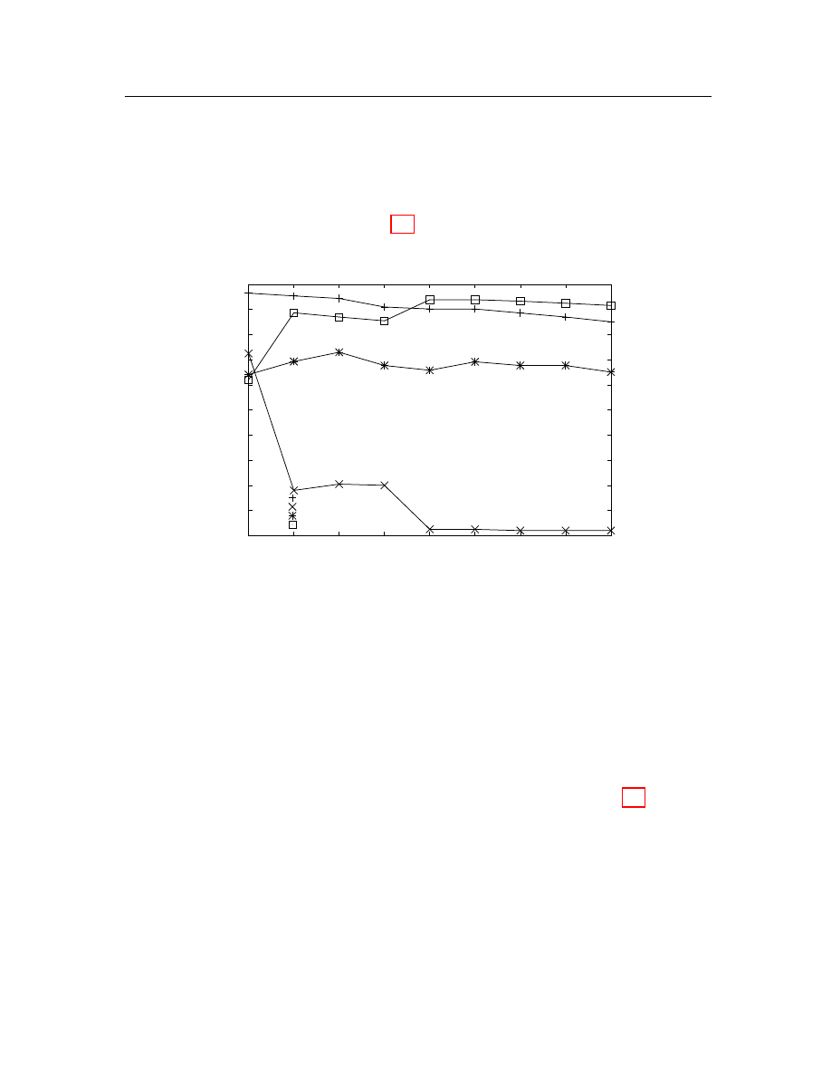
Chapter 5: Experiments and Performance Evaluation
53
reason that both 10-grams and 12-grams provide better false positive rates is still
the same. The merged feature list can reduce the number of features about 15% and
improve the false positive rate from 6% to roughly 2% while the detection rate drops
from 95% to 90%. Similar to Figure 5.4, experiments show that using an n-gram
length from 18 to 22 provides the highest accuracy.
1
0.9
0.8
0.7
0.6
0.5
0.4
0.3
0.2
0.1
0
24
22
20
18
16
14
12
10
8
Rate
Length of the N-gram
DR
FPR
IR
OAD
Figure 5.5: Double segments examination with merged features
Multiple segments examination
The result is comparatively better by check-
ing two successive segments, but what would the result be if checking more than
double segments for a session? If we examine more segments, we have to extract the
corresponding number of features from each family. One would hope that examining
more segments for a session would improve the result meaning a higher detection
rate and a lower false positive rate. However, our results (see Figure 5.6) are the
opposite of these expectations.
Both detection and identification rate drop after examining more than double
segments because of adding extra constraints when checking additional segments.
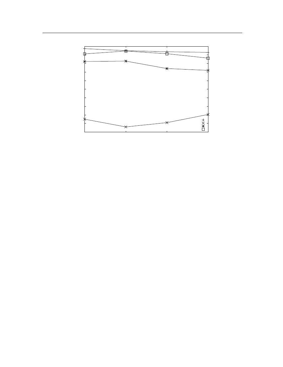
Chapter 5: Experiments and Performance Evaluation
54
0
0.1
0.2
0.3
0.4
0.5
0.6
0.7
0.8
0.9
1
4
3
2
1
Rate
Number of checked segments
DR
FPR
IR
OAD
Figure 5.6: Varying number of segments examined
The false positive rate increases because the quality of features is declining. In order
to examine more segments in the session, we have to extract more features from each
family. The most significant feature from each family is the longest common s-opcode
sequence. As we increases the number of features extracted from each family, the
quality (length) of features drops. Once the length of the feature falls too much, they
will become non-typical and start generating false alarms. Our results suggest that
checking double segments for each session gives the best result. It is not necessary
to go beyond this point.
Threshold selection
Overall, the results in the previous section show that the n-gram length from 18
to 22 provides the best accuracy regardless of the value of local alignment threshold.
Therefore, in this section, we arbitrarily select the n-gram length to be 18, and vary
the alignment threshold to appraise the system.
First, we test the system using the individual segment examination by changing
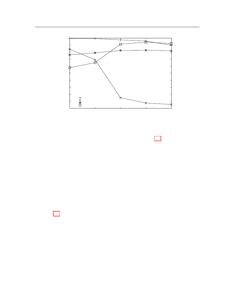
Chapter 5: Experiments and Performance Evaluation
55
0
0.1
0.2
0.3
0.4
0.5
0.6
0.7
0.8
0.9
1
1
0.9
0.8
0.7
0.6
Rate
The classifier threshold
DR
FPR
IR
OAD
Figure 5.7: Individual segment examination with varied alignment thresholds
the threshold. The experiment results are shown in Figure 5.7. The value of the
threshold varies from 0.6 to 1.0. Since we are using local alignment to measure
the similarity, reducing the threshold below 0.7 creates meaningless results. For
example, a 0.6 threshold gives a 99% detection rate, but it also reports 84% false
positives. If we further lower the threshold, both detection and false positive rates
will reach 100%. It is apparent that the smaller the value of the threshold is, the
higher the detection rate. However, the high detection rate results from false alerts
and therefore does not help improve the overall accuracy. We find that a threshold
of 0.9 gives the highest identification rate and best overall accuracy of detection.
Second, we vary the threshold for examining double segments. The result shown
in Figure 5.8 is very similar to the result of individual segment examination except it
illustrates a lower false positive rate. In general, experiments show that increasing the
threshold reduces the false positive rate, and the detection rate is decreased because
of severely increasing the threshold value. From results of both individual and double
segments examination, the experiments suggest that setting the threshold within the
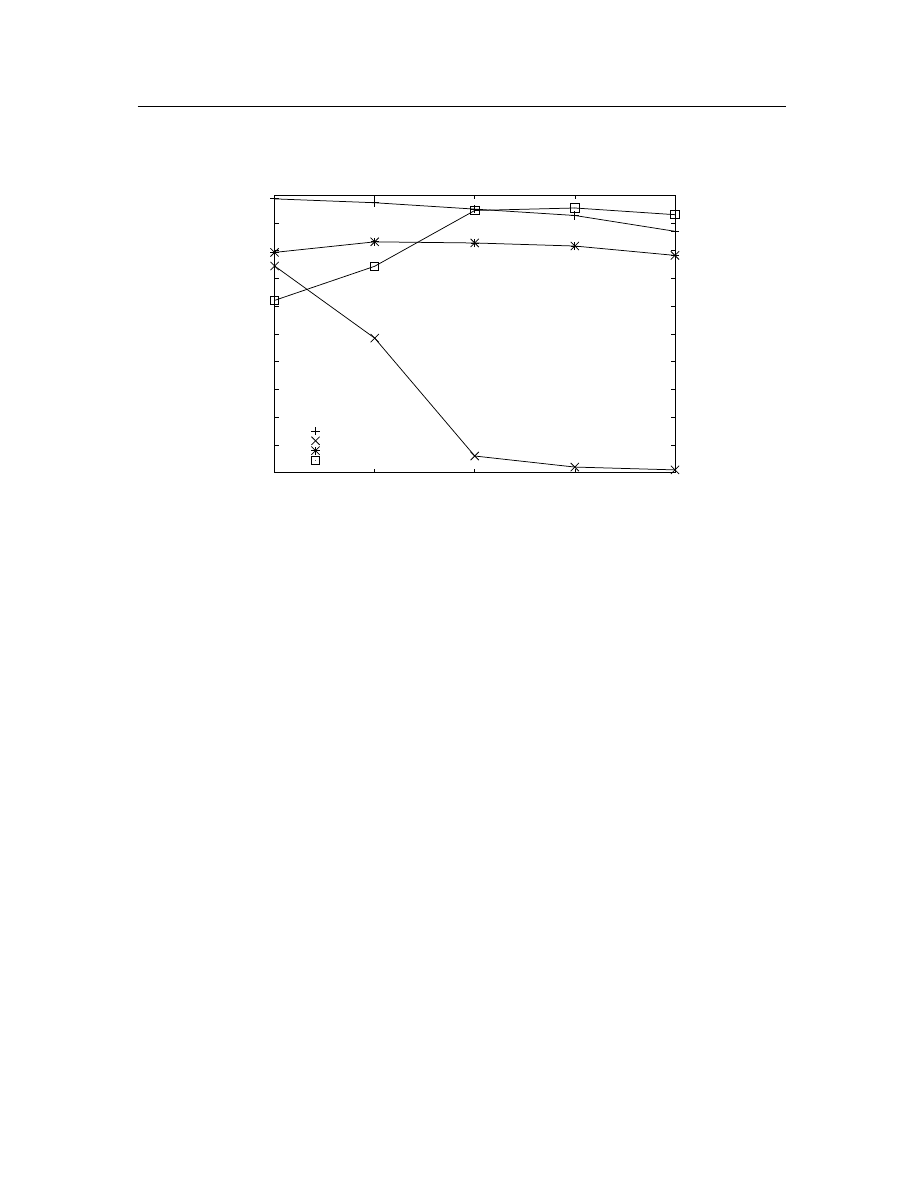
Chapter 5: Experiments and Performance Evaluation
56
range of 0.8 to 0.9 using double segments examination provides the highest accuracy.
0
0.1
0.2
0.3
0.4
0.5
0.6
0.7
0.8
0.9
1
1
0.9
0.8
0.7
0.6
Rate
The classifier threshold
DR
FPR
IR
OAD
Figure 5.8: Double segments examination with varied alignment thresholds
5.3.2.2
Experiments against the entire dataset
The experiments so far only test malicious executables from the training set. The
next step is to apply the features to all malicious executables. We randomly select
710 malicious executables as the training set which is 20% of the original dataset.
From previous experiments, the n-gram length of 18 and the threshold value of 0.8
generate the best overall accuracy. We apply these parameter values to double seg-
ments examination to detect executables from the entire dataset. The results show
that features generated this way can be used to achieve a detection rate of roughly
69.2% (2456/3548) while maintaining a 4.5% false positive rate. We definitely can
use a large training set to increase the final detection rate, but this is misleading.
In summary, our experiments suggest that double segments examination using a

Chapter 5: Experiments and Performance Evaluation
57
threshold within the range of 0.8 to 0.9 provides the highest accuracy, a 95% overall
accuracy of detection is possible and an identification rate of 83% can be achieved.

Chapter 6
Conclusions
In this thesis, we start with a hypothesis regarding the unique characteristics
among members in the same family of malicious X86 executables. Our whole project
is encircled with this assumption and we have applied techniques from data mining,
information retrieval and bioinformatics. Feature-based characteristics are employed
to solve the problems of detecting and identifying malicious executables. By intro-
ducing the automated identification system and the idea of extracting the “genetic”
information from malicious executables, our research differs from previous related
work that purely focuses on detection. The main contributions of our work can be
summarized as follows:
1. We treat malicious attacks as biological organisms by transforming binary ex-
ecutables into genome-like s-opcode sequences. Alignment algorithms from
bioinformatics and tools from other disciplines are combined in the training
and testing processes of our system.
2. In contrast to traditional two-class classification, we use one-class classification.
Exclusively examining the properties of malicious executables makes it possible
to classify both malicious and benign programs.
58

Chapter 6: Conclusions
59
3. Malicious samples are grouped into classes by the clustering algorithm. This
approach provides an opportunity to automatically group malicious attacks
instead of human experts.
4. Besides the problem of detecting malicious executables, our system also pro-
vides ways to identify unknown attacks by identifying their closest families.
Our approach provides an alternative view to the problem by using a combination
of many techniques to discover “genetic” features from malicious executables. Our
experimental results show that our system can accomplish an identification rate at
approximately 83% while achieving an overall detection rate of roughly 96%.
6.1
Limitations
Even though our system has relatively high accuracy, there are still limitations:
1. There are four parameters in the system, which we believe is too many. Some
of them are related to each other, but it is really complicated to control them
all. Although we propose boundaries for some of the parameters, lots of ex-
periments are still required in order to find the best values to achieve the best
results.
2. The feature list has to be rebuilt after a certain period of time after detecting
and identifying new attacks. If we want to distribute the features, when and
how to update them become the problem.
6.2
Future work
All limitations listed above are our future work, and there are still many places
for improvement.

Chapter 6: Conclusions
60
First, the clustering algorithm is not good enough.
In our experiments, the
identification rate is affected by the conjunction of distinct clusters. Since DBSCAN
cannot construct completely disjoint clusters, some families still contain very similar
features after clustering. A possible solution could either improve the clustering
algorithm or post-process the result clusters. We suggest proposing a threshold to
measure inter-family similarity. After clustering the samples, we can merge some of
the close families according to their similarities. Merging clusters could significantly
improve the quality of features in contrast to what we did in Section 5.3.2 by merging
the result features. However, the measurement of inter-family similarities is going to
introduce more parameters to the system.
Second, the present alignment scoring scheme is not very accurate. We are cur-
rently using the simplest pair-wise scoring scheme. The value -1 denotes that a
residue aligns with a different type of residue; the value -2 denotes that a residue
aligns to an empty spot; the value 1 means that a residue matches with the same
type of residue. In bioinformatics, researchers use better scoring matrixes such as
PAM [10] and BLOSUM [18] that are calculated statistically to measure the score
of the alignment. However, we do not have any supporting scoring matrix for the
alignment of s-opcode sequences. If we can build a scoring matrix based on the
sequence of malicious executables, it might improve the accuracy of our similarity
measurement.
Last, host-based security is not effective any more. Oberheide et al. propose a
distributed approach to subvert the architecture of current antivirus software [31].
By using the same concept, we could distribute the features of our system among
network devices such as routers and firewalls across the Internet. First, we could
deploy a special cache storing features in some network devices to examine network
traffic to prevent attacks before their arrival to hosts. If this scheme works, we
could further distribute this mechanism among all devices in the network. Instead
of containing all features, network devices could include a hierarchical distribution

Chapter 6: Conclusions
61
of the feature set. Distinct levels of the network could contain different levels of
features for blocking attacks with different severity. Features within each network
device do not have to be static. A feature-routing protocol could be designed for
devices to exchange features automatically according to their roles in the distributed
security system.

Bibliography
[1] Vx heavens. http://vx.netlux.org/.
[2] T. AbouAssaleh, N. Cercone, V. Keselj, and R. Sweidan. n-gram-based detection
of new malicious code. In COMPSAC ’04: Proceedings of the 28th Annual
International Computer Software and Applications Conference - Workshops and
Fast Abstracts - (COMPSAC’04), pages 41–42, Washington, DC, USA, 2004.
IEEE Computer Society. ISBN 0-7695-2209-2-2.
[3] A. V. Aho, R. Sethi, and J. Ullman. Compilers, Principles, Techniques, and
Tools. Addison-Wesley, 1986. ISBN 0-201-10088-6.
[4] J. Bergeron, M. Debbabi, J. Desharnais, M. M. Erhioui, Y. Lavoie, and
N. Tawbi. Static detection of malicious code in executable programs. Int. J. of
Req. Eng., 2001.
[5] B. Brors. An Introduction to Molecular Biotechnology. Wiley VCH, Weinheim,
Germany, 2006. ISBN 3-527-31412-1.
[6] A. D. M. Cai, J. Theiler, and M. Gokhale. Detecting a malicious executable
without prior knowledge of its patterns. In Proc. SPIE 5812, pages 1–12, 2005.
[7] S. Chapman. Similarity metric library. http://www.dcs.shef.ac.uk/ sam/stringmetrics.html.
[8] S. Coull, J. Branch, B. Szymanski, and E. Breimer. Intrusion detection: a
bioinformatics approach.
Computer Security Applications Conference, 2003.
Proceedings. 19th Annual, pages 24–33, Dec. 2003. doi: 10.1109/CSAC.2003.
1254307.
[9] DataRescue. IDA PRO 4.9 freeware. http://www.hex-rays.com/idapro/, 2008.
[10] M. O. Dayhoff, R. M. Schwartz, and B. C. Orcutt. A model of evolutionary
change in proteins. Atlas of protein sequence and structure, 5(suppl 3):345–351,
1978.
62

Bibliography
63
[11] P. S. Deng, J. Wang, W. Shieh, C. Yen, and C. Tung. Intelligent automatic
malicious code signatures extraction. Security Technology, 2003. Proceedings.
IEEE 37th Annual 2003 International Carnahan Conference, pages 600–603,
Oct. 2003.
[12] M. H. Dunham. Data Mining: Introductory and Advanced Topics. New Jersey:
Prentice Hall, 2003. ISBN 0-13-088892-3.
[13] M. Ester, H. P. Kriegel, J. Sander, and X. Xu. A density-based algorithm for
discovering clusters in large spatial databases with noise. pages 226–231. AAAI
Press, 1996.
[14] J. Euzenat and P. Shvaiko. Ontology matching. Springer-Verlag, 2007. ISBN
3-540-49611-4.
[15] M.
Fitzgerald.
The
future
of
antivirus.
http://www.pcadvisor.co.uk/news/index.cfm?newsid=12702, 2008.
[16] W. J. Frawley, P. G. Shapiro, and C. J. Matheus. Knowledge discovery in
databases - an overview. AI Magazine, 13:57–70, 1992.
[17] O. Henchiri and N. Japkowicz. A feature selection and evaluation scheme for
computer virus detection. In ICDM ’06: Proceedings of the Sixth International
Conference on Data Mining, pages 891–895, Washington, DC, USA, 2006. IEEE
Computer Society. ISBN 0-7695-2701-9.
[18] S. Henikoff and J. G. Henikoff. Amino acid substitution matrices from protein
blocks. Proceedings of the National Academy of Sciences(USA), 89(22):10915–
10919, November 1992. ISSN 0027-8424.
[19] D. Higgins, F. Sievers, and A. Wilm. CLUSTALW. http://www.clustal.org/.
[20] J. Huang and D. J. Lilja. Exploiting basic block value locality with block reuse.
High-Performance Computer Architecture, International Symposium on, 0:106,
1999.
[21] Intel.
Intel 64 and IA-32 architectures software developer’s manual.
http://www.intel.com/products/processor/manuals/index.htm.
[22] L. Kaufman and P. J. Rousseeuw. Finding Groups in Data: An Introduction to
Cluster Analysis. Wiley-Interscience, March 1990. ISBN 0-47-173578-7.

Bibliography
64
[23] J. O. Kephart and W. C. Arnold. Automatic extraction of computer virus
signatures. In Proceedings of the 4th Virus Bulletin International Conference,
pages 178–184, Virus Bulletin Ltd., Abingdon, England, 1994.
[24] J. Z. Kolter and M. A. Maloof. Learning to detect malicious executables in
the wild. In KDD ’04: Proceedings of the tenth ACM SIGKDD International
Conference on Knowledge Discovery and Data Mining, pages 470–478, New
York, NY, USA, 2004. ACM. ISBN 1-58113-888-1.
[25] J. Li, H. Liu, A. Tung, and L. Wong. Data mining techniques for the practical
bioinformatician. In L. Wong, editor, The Practical Bioinformatician, chapter 4,
pages 35–69. World Scientific, 2004.
[26] C. D. Manning and H. Sch¨
utze. Foundations of Statistical Natural Language
Processing. The MIT Press, June 1999. ISBN 0262133601.
[27] M. Masud, L. Khan, and B. Thuraisingham. A hybrid model to detect malicious
executables. pages 1443–1448. IEEE International Conference on Communica-
tions, 2007. ICC ’07, 2007.
[28] G. McGraw and G. Morrisett. Attacking malicious code: A report to the infosec
research council. IEEE Software., 17(5):33–41, 2000. ISSN 0740-7459.
[29] S. B. Needleman and C. D. Wunsch. A general method applicable to the search
for similarities in the amino acid sequence of two proteins. J Mol Biol, 48(3):
443–453, March 1970. ISSN 0022-2836.
[30] R. T. Ng and J. Han. Efficient and effective clustering methods for spatial data
mining. In 20th International Conference on Very Large Data Bases, September,
1994, Santiago, Chile, pages 144–155. Morgan Kaufmann Publishers, 1994.
[31] J. Oberheide, E. Cooke, and F. Jahanian. Rethinking antivirus: executable
analysis in the network cloud. In HOTSEC’07: Proceedings of the 2nd USENIX
workshop on Hot topics in security, pages 1–5, Berkeley, CA, USA, 2007.
USENIX Association.
[32] G. Salton and M. J. McGill. Introduction to Modern Information Retrieval.
McGraw-Hill, Inc., New York, NY, USA, 1986. ISBN 0070544840.
[33] M. G. Schultz, E. Eskin, E. Zadok, and S. J. Stolfo. Data mining methods for
detection of new malicious executables. In SP ’01: Proceedings of the 2001 IEEE

Bibliography
65
Symposium on Security and Privacy, pages 38–49, Washington, DC, USA, 2001.
IEEE Computer Society.
[34] E. Skoudis and L. Ziltser. Malware: Fighting Malicious Code. New Jersey:
Prentice Hall, 2003. ISBN 0-131-01405-6.
[35] T. F. Smith and M. S. Waterman. Identification of common molecular subse-
quences. Journal of Molecular Biology, 147(1):195–197, March 1981.
[36] K. Takeda. The application of bioinformatics to network intrusion detection. Se-
curity Technology, 2005. CCST ’05. 39th Annual 2005 International Carnahan
Conference, pages 130–132, Oct. 2005. doi: 10.1109/CCST.2005.1594860.
[37] J. D. Thompson, D. G. Higgins, and T. J. Gibson. Clustal w: improving the
sensitivity of progressive multiple sequence alignment through sequence weight-
ing, position-specific gap penalties and weight matrix choice. Nucleic Acids Res,
22(22):4673–4680, November 1994. ISSN 0305-1048.
[38] J. Wang, P. Deng, Y. Fan, L. Jaw, and Y. Liu. Virus detection using data
mining techinques. Security Technology, 2003. Proceedings. IEEE 37th Annual
2003 International Carnahan Conference, pages 71–76, Oct. 2003.
[39] S. R. White. Open problems in computer virus research. Germany, 1998. Virus
Bulletin Conference.
[40] W. Wien. R project for statistical computing. http://www.r-project.org/.
[41] B. Zhang, J. Yin, J. Hao, D. Zhang, and S. Wang. Using support vector machine
to detect unknown computer viruses. International Journal of Computational
Intelligence Research, 2(2):100–104, November 2006. ISSN 0973-1873.

Appendix A
Intel opcode grouping
This section is the detailed table to illustrate how we group about two hundreds
of Intel opcode. According to Intel
R
IA-32 Architectures Software Developer’s Man-
ual from [21], general purpose opcodes are grouped into 13 groups. With a slight
modification, we group all the opcodes into 11 groups.
Intel group
Opcode
Our group
Data Transfer
MOV
Data Transfer(D)
Data Transfer
CMOVE
Data Transfer(D)
Data Transfer
CMOVZ
Data Transfer(D)
Data Transfer
CMOVNE
Data Transfer(D)
Data Transfer
CMOVNZ
Data Transfer(D)
Data Transfer
CMOVA
Data Transfer(D)
Data Transfer
CMOVNBE
Data Transfer(D)
Data Transfer
CMOVAE
Data Transfer(D)
Data Transfer
CMOVNB
Data Transfer(D)
Data Transfer
CMOVB
Data Transfer(D)
Data Transfer
CMOVNAE
Data Transfer(D)
Data Transfer
CMOVBE
Data Transfer(D)
Data Transfer
CMOVNA
Data Transfer(D)
Data Transfer
CMOVG
Data Transfer(D)
Data Transfer
CMOVNLE
Data Transfer(D)
Data Transfer
CMOVGE
Data Transfer(D)
Data Transfer
CMOVNL
Data Transfer(D)
Data Transfer
CMOVL
Data Transfer(D)
Continued on next page
66

Appendix A: Intel opcode grouping
67
Table A.1 continued from previous page
Intel group
Opcode
Our group
Data Transfer
CMOVNGE
Data Transfer(D)
Data Transfer
CMOVLE
Data Transfer(D)
Data Transfer
CMOVNG
Data Transfer(D)
Data Transfer
CMOVC
Data Transfer(D)
Data Transfer
CMOVNC
Data Transfer(D)
Data Transfer
CMOVO
Data Transfer(D)
Data Transfer
CMOVNO
Data Transfer(D)
Data Transfer
CMOVS
Data Transfer(D)
Data Transfer
CMOVNS
Data Transfer(D)
Data Transfer
CMOVP
Data Transfer(D)
Data Transfer
CMOVPE
Data Transfer(D)
Data Transfer
CMOVNP
Data Transfer(D)
Data Transfer
CMOVPO
Data Transfer(D)
Data Transfer
XCHG
Data Transfer(D)
Data Transfer
BSWAP
Data Transfer(D)
Data Transfer
XADD
Data Transfer(D)
Data Transfer
CMPXCHG
Data Transfer(D)
Data Transfer
CMPXCHG8B
Data Transfer(D)
Data Transfer
PUSH
Data Transfer(D)
Data Transfer
POP
Data Transfer(D)
Data Transfer
PUSHA
Data Transfer(D)
Data Transfer
PUSHAD
Data Transfer(D)
Data Transfer
POPA
Data Transfer(D)
Data Transfer
POPAD
Data Transfer(D)
Data Transfer
CWD
Data Transfer(D)
Data Transfer
CDQ
Data Transfer(D)
Data Transfer
CBW
Data Transfer(D)
Data Transfer
CWDE
Data Transfer(D)
Data Transfer
MOVSX
Data Transfer(D)
Data Transfer
MOVZX
Data Transfer(D)
Binary Arithmetic
ADD
Arithmetic(A)
Binary Arithmetic
ADC
Arithmetic(A)
Binary Arithmetic
SUB
Arithmetic(A)
Binary Arithmetic
SBB
Arithmetic(A)
Continued on next page

Appendix A: Intel opcode grouping
68
Table A.1 continued from previous page
Intel group
Opcode
Our group
Binary Arithmetic
IMUL
Arithmetic(A)
Binary Arithmetic
MUL
Arithmetic(A)
Binary Arithmetic
IDIV
Arithmetic(A)
Binary Arithmetic
DIV
Arithmetic(A)
Binary Arithmetic
INC
Arithmetic(A)
Binary Arithmetic
DEC
Arithmetic(A)
Binary Arithmetic
NEG
Arithmetic(A)
Binary Arithmetic
CMP
Arithmetic(A)
Decimal Arithmetic
DAA
Arithmetic(A)
Decimal Arithmetic
DAS
Arithmetic(A)
Decimal Arithmetic
AAA
Arithmetic(A)
Decimal Arithmetic
AAS
Arithmetic(A)
Decimal Arithmetic
AAM
Arithmetic(A)
Decimal Arithmetic
AAD
Arithmetic(A)
Logical
AND
Logical(L)
Logical
OR
Logical(L)
Logical
XOR
Logical(L)
Logical
NOT
Logical(L)
Shift and Rotate
SAR
Shift and Rotate(T)
Shift and Rotate
SHR
Shift and Rotate(T)
Shift and Rotate
SAL
Shift and Rotate(T)
Shift and Rotate
SHL
Shift and Rotate(T)
Shift and Rotate
SHRD
Shift and Rotate(T)
Shift and Rotate
SHLD
Shift and Rotate(T)
Shift and Rotate
ROR
Shift and Rotate(T)
Shift and Rotate
ROL
Shift and Rotate(T)
Shift and Rotate
RCR
Shift and Rotate(T)
Shift and Rotate
RCL
Shift and Rotate(T)
Bit and Byte
BT
Bit and Byte(H)
Bit and Byte
BTS
Bit and Byte(H)
Bit and Byte
BTR
Bit and Byte(H)
Bit and Byte
BTC
Bit and Byte(H)
Continued on next page

Appendix A: Intel opcode grouping
69
Table A.1 continued from previous page
Intel group
Opcode
Our group
Bit and Byte
BSF
Bit and Byte(H)
Bit and Byte
BSR
Bit and Byte(H)
Bit and Byte
SETE
Bit and Byte(H)
Bit and Byte
SETZ
Bit and Byte(H)
Bit and Byte
SETNE
Bit and Byte(H)
Bit and Byte
SETNZ
Bit and Byte(H)
Bit and Byte
SETA
Bit and Byte(H)
Bit and Byte
SETNBE
Bit and Byte(H)
Bit and Byte
SETAE
Bit and Byte(H)
Bit and Byte
SETNB
Bit and Byte(H)
Bit and Byte
SETNC
Bit and Byte(H)
Bit and Byte
SETB
Bit and Byte(H)
Bit and Byte
SETNAE
Bit and Byte(H)
Bit and Byte
SETC
Bit and Byte(H)
Bit and Byte
SETBE
Bit and Byte(H)
Bit and Byte
SETNA
Bit and Byte(H)
Bit and Byte
SETG
Bit and Byte(H)
Bit and Byte
SETNLE
Bit and Byte(H)
Bit and Byte
SETGE
Bit and Byte(H)
Bit and Byte
SETNL
Bit and Byte(H)
Bit and Byte
SETL
Bit and Byte(H)
Bit and Byte
SETNGE
Bit and Byte(H)
Bit and Byte
SETLE
Bit and Byte(H)
Bit and Byte
SETNG
Bit and Byte(H)
Bit and Byte
SETS
Bit and Byte(H)
Bit and Byte
SETNS
Bit and Byte(H)
Bit and Byte
SETO
Bit and Byte(H)
Bit and Byte
SETNO
Bit and Byte(H)
Bit and Byte
SETPE
Bit and Byte(H)
Bit and Byte
SETP
Bit and Byte(H)
Bit and Byte
SETPO
Bit and Byte(H)
Bit and Byte
SETNP
Bit and Byte(H)
Bit and Byte
TEST
Bit and Byte(H)
Control
JMP
Control(C)
Continued on next page

Appendix A: Intel opcode grouping
70
Table A.1 continued from previous page
Intel group
Opcode
Our group
Control
JE
Control(C)
Control
JZ
Control(C)
Control
JNE
Control(C)
Control
JNZ
Control(C)
Control
JA
Control(C)
Control
JNBE
Control(C)
Control
JAE
Control(C)
Control
JNB
Control(C)
Control
JB
Control(C)
Control
JNAE
Control(C)
Control
JBE
Control(C)
Control
JNA
Control(C)
Control
JG
Control(C)
Control
JNLE
Control(C)
Control
JGE
Control(C)
Control
JNL
Control(C)
Control
JL
Control(C)
Control
JNGE
Control(C)
Control
JLE
Control(C)
Control
JNG
Control(C)
Control
JC
Control(C)
Control
JNC
Control(C)
Control
JO
Control(C)
Control
JNO
Control(C)
Control
JS
Control(C)
Control
JNS
Control(C)
Control
JPO
Control(C)
Control
JNP
Control(C)
Control
JPE
Control(C)
Control
JP
Control(C)
Control
JCXZ
Control(C)
Control
JECXZ
Control(C)
Control
LOOP
Control(C)
Control
LOOPZ
Control(C)
Control
LOOPE
Control(C)
Continued on next page

Appendix A: Intel opcode grouping
71
Table A.1 continued from previous page
Intel group
Opcode
Our group
Control
LOOPNZ
Control(C)
Control
LOOPNE
Control(C)
Control
CALL
Control(C)
Control
RET
Control(C)
Control
IRET
Control(C)
Control
INT
Control(C)
Control
INTO
Control(C)
Control
BOUND
Control(C)
Control
ENTER
Control(C)
Control
LEAVE
Control(C)
Control
RETF
Control(C)
String
MOVS
String(S)
String
MOVSB
String(S)
String
MOVS
String(S)
String
MOVSW
String(S)
String
MOVS
String(S)
String
MOVSD
String(S)
String
CMPS
String(S)
String
CMPSB
String(S)
String
CMPS
String(S)
String
CMPSW
String(S)
String
CMPS
String(S)
String
CMPSD
String(S)
String
SCAS
String(S)
String
SCASB
String(S)
String
SCAS
String(S)
String
SCASW
String(S)
String
SCAS
String(S)
String
SCASD
String(S)
String
LODS
String(S)
String
LODSB
String(S)
String
LODS
String(S)
String
LODSW
String(S)
String
LODS
String(S)
Continued on next page

Appendix A: Intel opcode grouping
72
Table A.1 continued from previous page
Intel group
Opcode
Our group
String
LODSD
String(S)
String
STOS
String(S)
String
STOSB
String(S)
String
STOS
String(S)
String
STOSW
String(S)
String
STOS
String(S)
String
STOSD
String(S)
String
REP
String(S)
String
REPE
String(S)
String
REPZ
String(S)
String
REPNE
String(S)
String
REPNZ
String(S)
I/O
IN
I/O(I)
I/O
OUT
I/O(I)
I/O
INS
I/O(I)
I/O
INSB
I/O(I)
I/O
INS
I/O(I)
I/O
INSW
I/O(I)
I/O
INS
I/O(I)
I/O
INSD
I/O(I)
I/O
OUTS
I/O(I)
I/O
OUTSB
I/O(I)
I/O
OUTS
I/O(I)
I/O
OUTSW
I/O(I)
I/O
OUTS
I/O(I)
I/O
OUTSD
I/O(I)
Flag Control
STC
Flag Control(F)
Flag Control
CLC
Flag Control(F)
Flag Control
CMC
Flag Control(F)
Flag Control
CLD
Flag Control(F)
Flag Control
STD
Flag Control(F)
Flag Control
LAHF
Flag Control(F)
Flag Control
SAHF
Flag Control(F)
Continued on next page

Appendix A: Intel opcode grouping
73
Table A.1 continued from previous page
Intel group
Opcode
Our group
Flag Control
PUSHF
Flag Control(F)
Flag Control
PUSHFD
Flag Control(F)
Flag Control
POPF
Flag Control(F)
Flag Control
POPFD
Flag Control(F)
Flag Control
STI
Flag Control(F)
Flag Control
CLI
Flag Control(F)
Segment Register
LDS
Segment Register(R)
Segment Register
LES
Segment Register(R)
Segment Register
LFS
Segment Register(R)
Segment Register
LGS
Segment Register(R)
Segment Register
LSS
Segment Register(R)
Miscellaneous
LEA
Miscellaneous(M)
Miscellaneous
NOP
Miscellaneous(M)
Miscellaneous
XLAT
Miscellaneous(M)
Miscellaneous
XLATB
Miscellaneous(M)
Miscellaneous
CPUID
Miscellaneous(M)
Miscellaneous
MOVBE
Miscellaneous(M)
Table A.1: Opcode grouping
There is one group, Enter and Leave Instructions, from Intel manual that only
contains two instructions, ENTER and LEAVE. Both of the ENTER and LEAVE
instructions appear in the group of Control Transfer Instructions as well. According
to their functionality, we ignore this group and categorize both instructions into the
group of Control Transfer. Therefore, we obtain eleven groups by ignoring one group
and combining Binary and Decimal Arithmetic groups into one.

Appendix B
numerical experimental results
This appendix contains a list of tables with experimental results referring to
graphs in Chapter 5.
N -gram
8
10
12
14
16
18
20
22
24
DR
1
1
0.979
0.979
0.976
0.973
0.975
0.973
0.973
FPR
0.845
0.845
0.73
0.725
0.165
0.13
0.13
0.115
0.11
IR
0.717
0.689
0.807
0.814
0.786
0.823
0.828
0.789
0.82
OAD
0.578
0.578
0.625
0.627
0.906
0.922
0.923
0.929
0.932
Table B.1:
Numerical results for individual segment examination referring to Fig-
ure 5.2.
N -gram
8
10
12
14
16
18
20
22
24
DR
0.976
0.939
0.938
0.952
0.931
0.928
0.928
0.921
0.925
FPR
0.835
0.490
0.545
0.57
0.12
0.12
0.1
0.095
0.095
IR
0.654
0.69
0.704
0.71
0.682
0.71
0.703
0.677
0.708
OAD
0.571
0.725
0.697
0.691
0.906
0.904
0.914
0.913
0.915
Table B.2: Numerical results for individual segment examination using the merged
feature list referring Figure 5.3.
74

Appendix B: numerical experimental results
75
N -gram
8
10
12
14
16
18
20
22
24
DR
0.994
0.99
0.979
0.97
0.95
0.95
0.951
0.946
0.945
FPR
0.735
0.73
0.485
0.48
0.06
0.06
0.045
0.045
0.04
IR
0.718
0.69
0.763
0.765
0.803
0.828
0.752
0.792
0.797
OAD
0.63
0.63
0.747
0.745
0.945
0.945
0.953
0.951
0.953
Table B.3:
Numerical results for double segments examination referring to Fig-
ure 5.4.
N -gram
8
10
12
14
16
18
20
22
24
DR
0.965
0.954
0.944
0.91
0.902
0.902
0.886
0.87
0.851
FPR
0.725
0.18
0.205
0.2
0.025
0.025
0.02
0.02
0.02
IR
0.641
0.693
0.73
0.677
0.658
0.692
0.677
0.677
0.651
OAD
0.62
0.887
0.87
0.855
0.939
0.939
0.933
0.925
0.916
Table B.4:
Numerical results for double segments examination using the merged
feature list referring to Figure 5.5.
Number of segments
1
2
3
4
DR
0.973
0.95
0.937
0.93
FPR
0.15
0.06
0.11
0.205
IR
0.823
0.828
0.741
0.72
OAD
0.912
0.945
0.914
0.863
Table B.5: Numerical results for varying the number of examining segments referring
to Figure 5.6.

Appendix B: numerical experimental results
76
Threshold
60%
70%
80%
90%
100%
DR
0.994
0.992
0.973
0.958
0.896
FPR
0.84
0.69
0.13
0.075
0.055
IR
0.761
0.789
0.823
0.827
0.818
OAD
0.577
0.651
0.922
0.942
0.921
Table B.6: Numerical results for varying classifier threshold for one segment exam-
ination referring to Figure 5.7.
Threshold
60%
70%
80%
90%
100%
DR
0.987
0.973
0.95
0.927
0.87
FPR
0.745
0.485
0.06
0.02
0.01
IR
0.794
0.832
0.828
0.817
0.783
OAD
0.621
0.744
0.945
0.954
0.93
Table B.7:
Numerical results for varying classifier threshold for double segments
examination referrring to Figure 5.8.
Document Outline
- Dedication
- Abstract
- Table of Contents
- List of Figures
- List of Tables
- Acknowledgments
- Introduction
- Related work
- Background
- Malicious code detection and identification
- Experiments and Performance Evaluation
- Conclusions
- Bibliography
- Intel opcode grouping
- numerical experimental results
Wyszukiwarka
Podobne podstrony:
6 6 Detection and Identification of Drugs; Summary
Data Mining Methods for Detection of New Malicious Executables
Advances in the Detection and Diag of Oral Precancerous, Cancerous Lesions [jnl article] J Kalmar (
Detection and Function of Opioid Receptors on Cells from the Immune System
Sexualities and Identities of Minority Women
Generic Detection and Classification of Polymorphic Malware Using Neural Pattern Recognition
Szczepanik, Renata Development and Identity of Penitentiary Education (2012)
Static Detection of Malicious Code in Executable Programs
Learning to Detect and Classify Malicious Executables in the Wild
System and method for detecting malicious executable code
feminism and formation of ethnic identity in greek culture
Learning to Detect Malicious Executables in the Wild
Detection and Molecular Characterization of 9000 Year Old Mycobacterium tuberculosis from a Neolithi
feminism and formation of ethnic identity in greek culture
Supervisory control of malicious executables
Formalisation and implementation aspects of K ary (malicious) codes
Identification of inorganic pigments from paintings and ~56F
więcej podobnych podstron