
arXiv:hep-th/0111275 v1 29 Nov 2001
String Cosmology
Nick E. Mavromatos
King’s College London, Department of Physics,
Theoretical Physics, Strand, London WC2R 2LS, U.K.
Abstract
“Old’ String Theory is a theory of one-dimensional extended objects, whose vibrations corre-
spond to excitations of various target-space field modes including gravity. It is for this reason that
strings present the first, up to now, mathematically consistent framework where quantum gravity
is unified with the rest of the fundamental interactions in nature. In these lectures I will give
an introduction to low-energy Effective Target-Space Actions derived from conformal invariance
conditions of the underlying sigma models in string theory. In this context, I shall discuss cos-
mology, emphasizing the role of the dilaton field in inducing inflationary scenaria and in general
expanding string universes. Specifically, I shall analyse some exact solutions of string theory with
a linear dilaton, and discuss their role in inducing expanding Robertson-Walker Universes. I will
mention briefly pre-Big-Bang scenaria of String Cosmology, in which the dilaton plays a crucial
role. In view of recent claims on experimental evidence (from diverse astrophysical sources) on
the existence of cosmic acceleration in the universe today, with a positive non-zero cosmological
constant (de Sitter type), I shall also discuss difficulties of incorporating such Universes with
eternal acceleration in the context of critical string theory, and present scenaria for a graceful
exit from such a phase.
Lectures presented at the First Aegean Summer School on Cosmology, Karlovassi
(Samos), Greece, September 21-19 2001.
1
Introduction
Our way of thinking towards an understanding of the fundamental forces in nature, as well
as of the structure of matter and that of space time, has evolved over the last decades
of the previous century from that of using point-like structures as the basic constituents
of matter, to that employing one-dimensional extended objects (strings [1]), and, recently
(from the mid 90’s), higher-dimensional domain-wall like solitonic objects, called (Dirichlet)
(mem)branes [2].
The passage from point-like fundamental constituents to strings, in the mid 1980’s,
has already revolutionarized our view of space time and of the unification of fundamental
interactions in Nature, including gravity. Although in the framework of point-like field
theories, the uncontrollable ultraviolet (short-distance) divergencies of quantum gravity
prevented the development of a mathematically consistent unifying theory of all known
interactions in Nature, the discovery of one-dimensional fundamental constituents of matter
and space-time, called strings, which were in principle free from such divergenecies, opened
up the way for a mathematically cosistent way of incorporating quantum gravity on an
equal footing with the rest of the interactions. The existence of a minimum length `
s
in
string theory, in such a way that the quantum uncertainty principle between position X
and momenta P : ∆X∆P
≥ ¯h, of point-like quantum mechanics is replaced by: ∆X ≥
`
s
,
∆X∆P
≥ ¯h + O(`
2
s
)∆P
2
+ . . ., revolutionaized the way we looked at the structure
of space time at such small scales. The unification of gravitaional interactions with the
rest is achieved in this framework if one identifies the string scale `
s
with the Planck scale,
`
P
= 10
−35
m, where gravitational interactions are expected to set in. The concept of space
time, as we preceive it, breaks down beyond the string (Planck) scale, and thus there is a
fundamental short-distance cutoff built-in in the theory, which results in its finiteness.
The cost, however, for such an achievement, was that mathematical consistency implied
a higher-dimensional target space time, in which the strings propagate. This immediately
lead the physicists to try and determine the correct vacuum configurations of string theory
which would result into a four-dimensional Universe, i.e. a Universe with four dimensions
being “large” compared to the gravitational scale, the Planck length, 10
−35
m, with the
extra dimensions compactified on Planckian size manifolds. Unfortunately such consistent
ground states are not unique, and there is a huge degeneracy among such string vacua, the
lifitng of which is still an important unresolved problem in string physics.
In the last half of the 1990’s the discovery of string dualities, i.e. discrete stringy (non-
perturbative) gauge symmetries linking various string theories, showed another interesting
possibility, which could contribute significantly towards the elimination of the huge degen-
eracy problem of the string vacua. Namely, many string theories were found to be dual
to each other in the sense of exhibiting invariances of their physical spectra of excitations
under the action of such discrete symmetries. In fact, by virtue of such dualities one
could argue that there exist a sort of unification of string theories, in which all the known
string theories (type IIA, type IIB, SO(32)/Z
2
, Heterotic E
8
× E
8
, type I), together with
11 dimensional supergavity (living in one-dimension higher than the critical dimension of
superstrings) can be all connected with string dualities, so that one may view them as low
1

energy limits of a mysterious larger theory, termed M -theory [2], whose precise dynamics
is still not known.
A crucial rˆole in such string dualities is played by domain walls, stringy solitons, which
can be derived from ordinary strings upon the application of such dualities. Such extended
higher-dimensional objects are also excitations of this mysterious M-theory, and they are
on a completely equal footing with their one dimensional (stringy) counterparts.
In this framework one could discuss cosmology. The latter is nothing other but a theory
of the gravitational field, in which the Universe is treated as a whole. As such, string or M-
theory theory, which includes the gravitational field in its spectrum of excitations, seems the
appropriate framework for providing analyses on issues of the Early Universe Cosmology,
such as the nature of the initial singularity (Big Bang), the inflationary phase and graceful
exit from it etc, which conventional local field theories cannot give a reliable answer to.
It is the purpose of this lectures to provide a very brief, but hopefully comprehensive
discussion, on String Cosmology. We use the terminoloy string cosmology here to discuss
Cosmology based on one-dimensional fundamental constituents (strings). Cosmology may
also be discussed from the more modern point of view of membrane structures in M-
theory, mentioned above, but this will not be covered in these lectures. Other lecturers in
the School will discuss this issue.
The structure of the lectures is as follows: in the first lecture we shall introduce the
layman into the subject of string effective actions, and discuss how equations of motion
of the various low-energy modes of strings are associated with fundamental consistency
properties (conformal invariance) of the underlying string theory. In the second lecture
we shall discuss various scenaria for String Cosmology, together with their physical conse-
quences. Specifically I will discuss how expanding and inflationary (de Sitter) Universes are
incorporated in string theory, with emphasis on describing new fatures, not characterizing
conventional point-like cosmologies. Finally, in the third lecture we shall speculate on ways
of providing possible resolution to various theoretical challenges for string theory, especially
in view of recent astrophysical evidence of a current-era acceleration of our Universe. In
this respect we shall discuss the application of the so-called non-critical (Liouville) string
theory to cosmology, as a way of going off equilibrium in a string-theory setting, in analogy
with the use of non-equilibrium field theories in conventional point-like cosmological field
theories of the Early Universe.
2
Lecture 1: Introduction to String Effective Actions
2.1
World-sheet String formalism
In this lectures the terminology “string theory” will be restricted to the “old” concept of
one (spatial) dimensional extended objects, propagating in target-space times of dimensions
higher than four, specifically 26 for Bosonic strings and 10 for Super(symmetric)strings.
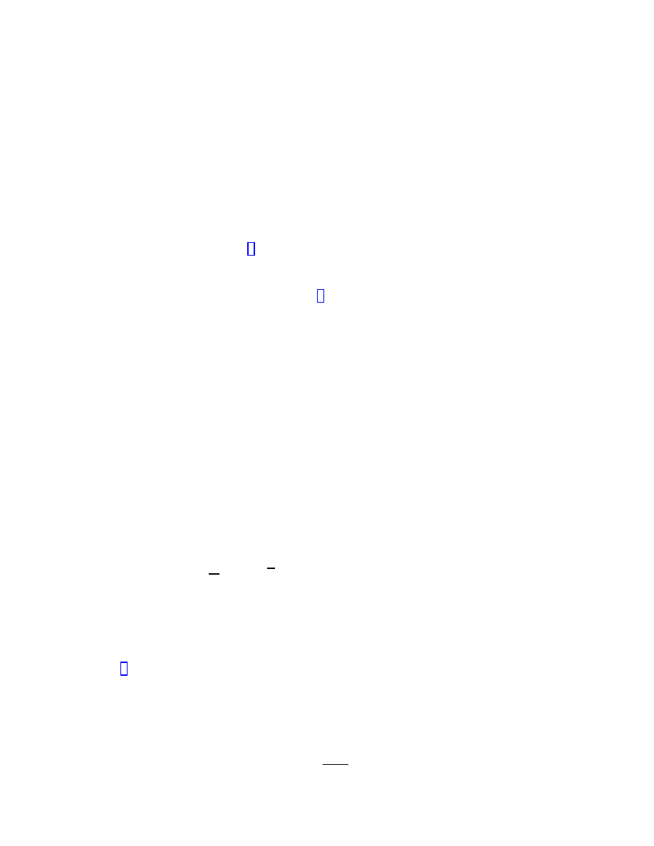
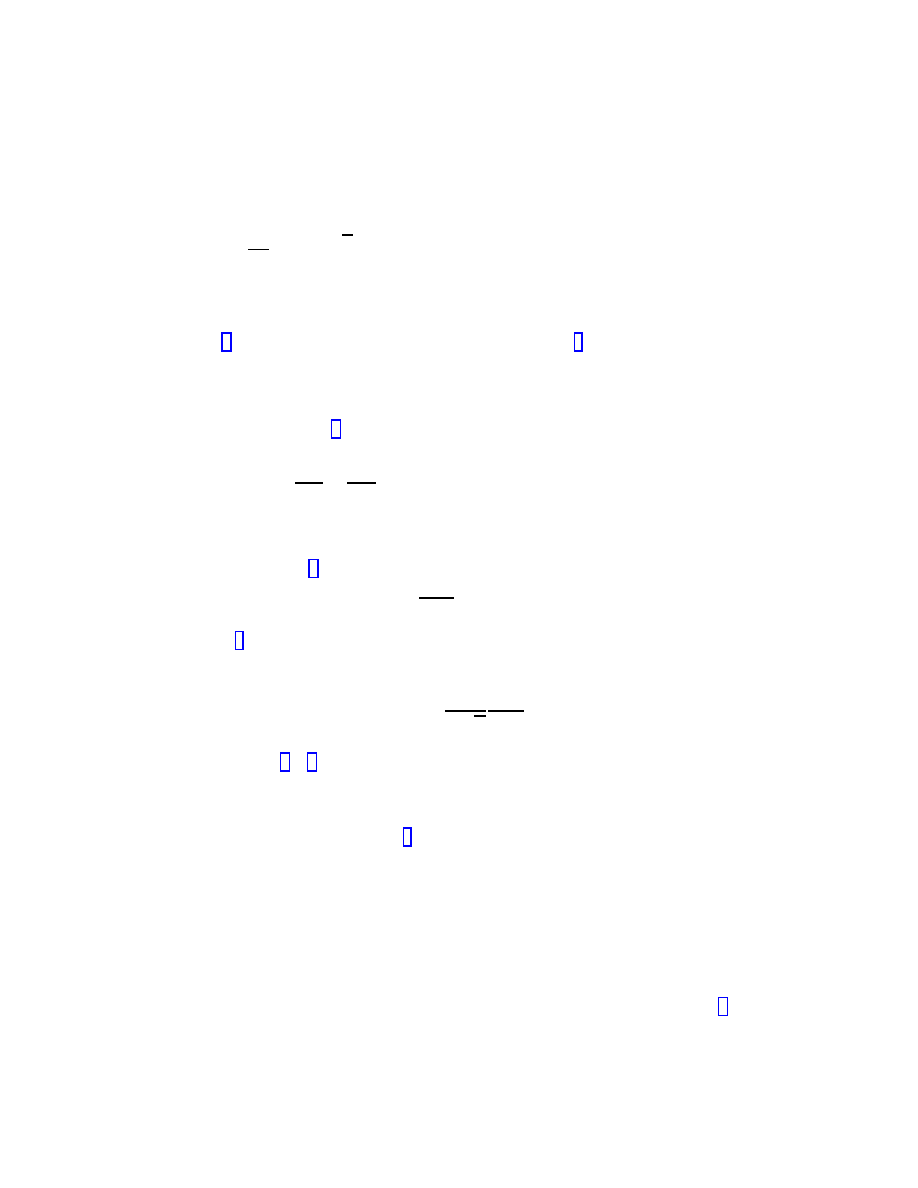
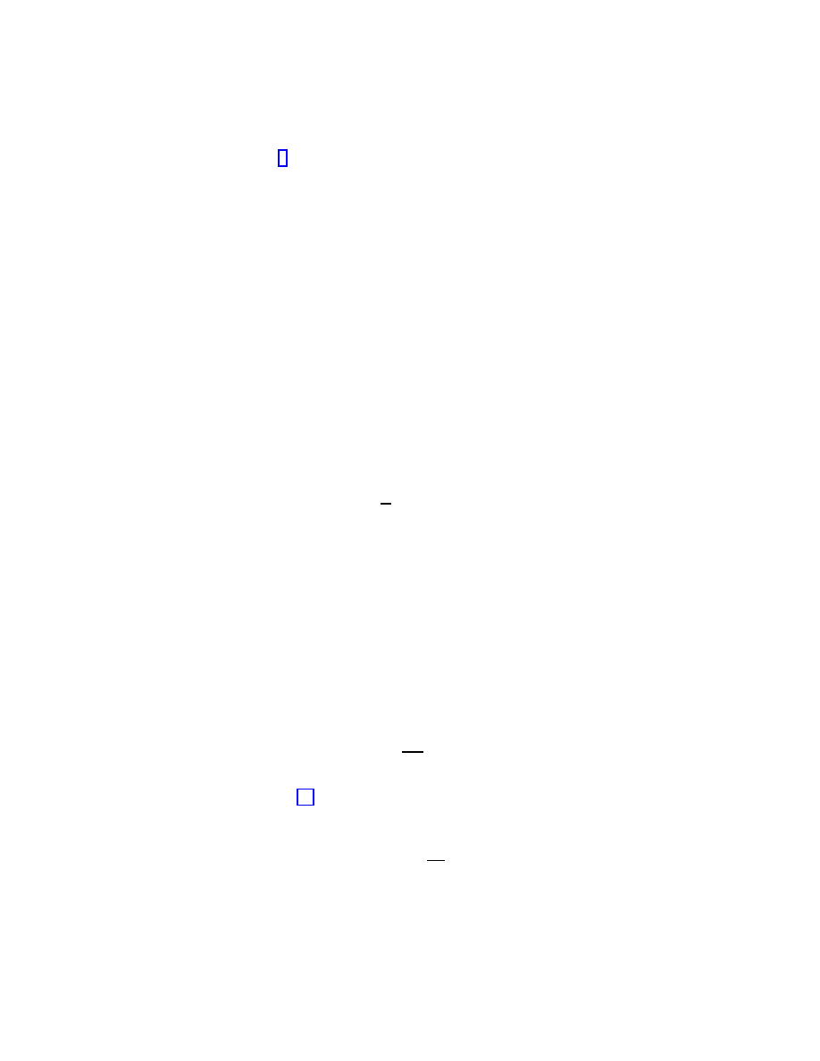
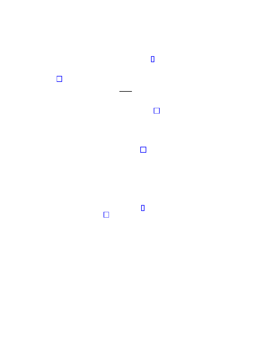
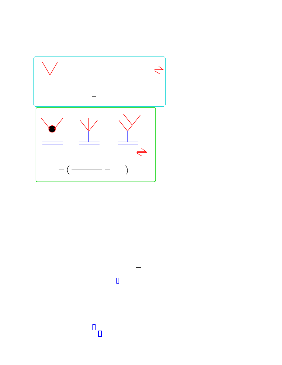
There are in general two types of such objects, as illustrated in a self-explanatory way in
figure 1: open strings and closed strings. In the first quantized formalism, one is interested
2
in the propagation of such extended objects in a background space time. By direct exten-
sion of the concept of a point-particle, the motion of a string as it glides through spacetime
is described by the world sheet, a two dimensional Riemann surface which is swept by the
extended object during its propagation through spacetime. The world-sheet is a direct ex-
tension of the concept of the world line in the case of a point particle. The important formal
difference of the string case, as compared with the particle one, is the fact that quantum
corrections, i.e. string loops, are incorporated in a smooth and straightforward manner
in the case of string theory by means of summing over Riemann surfaces with non-trivial
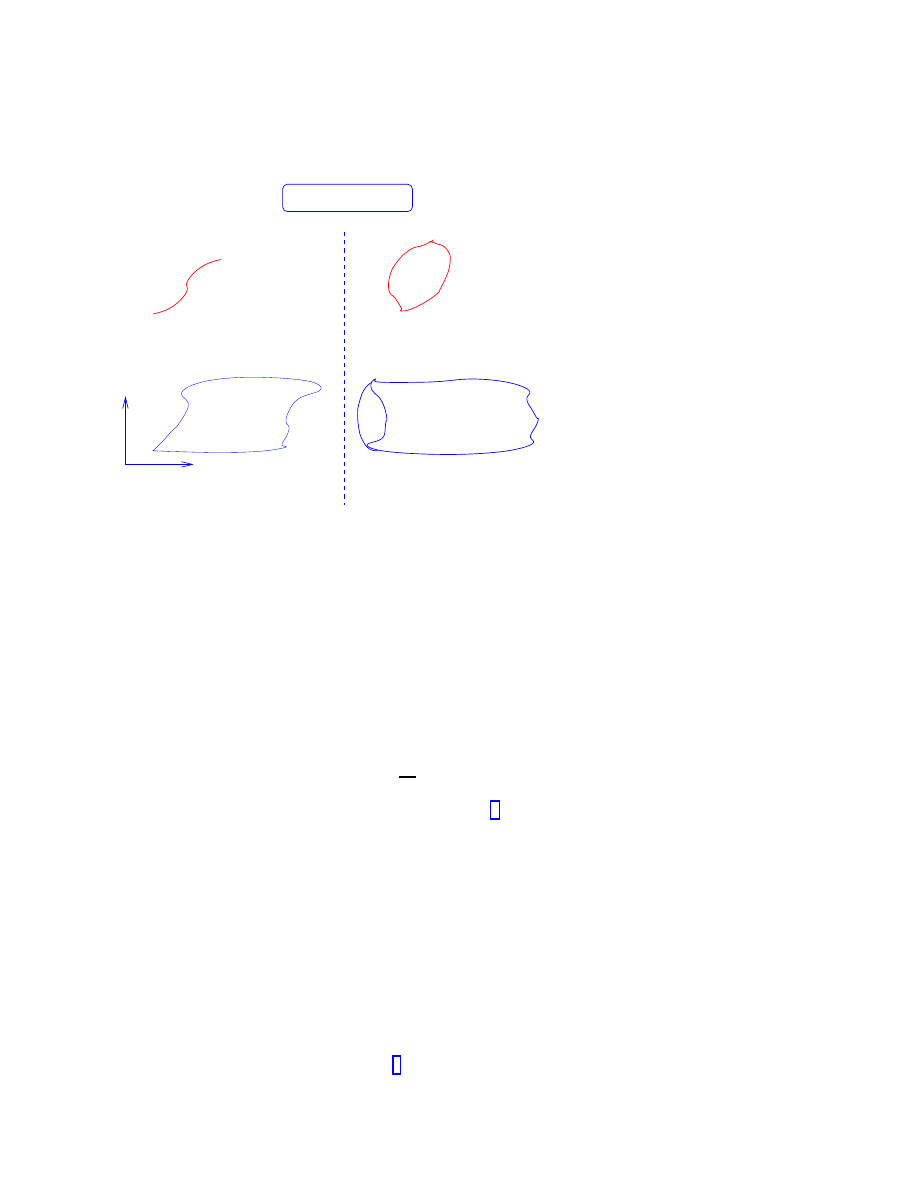
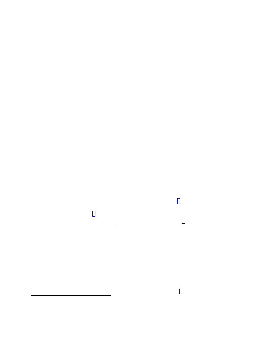
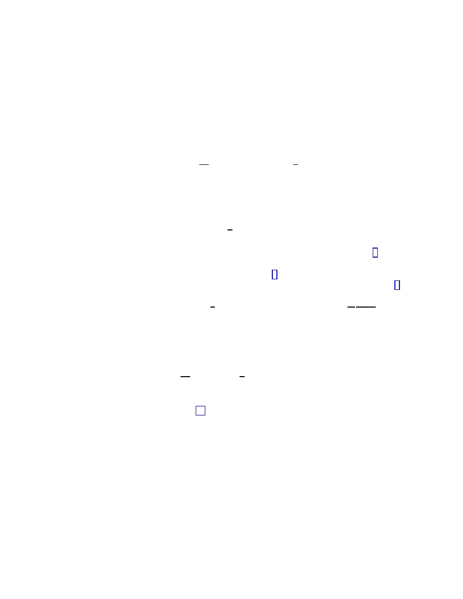
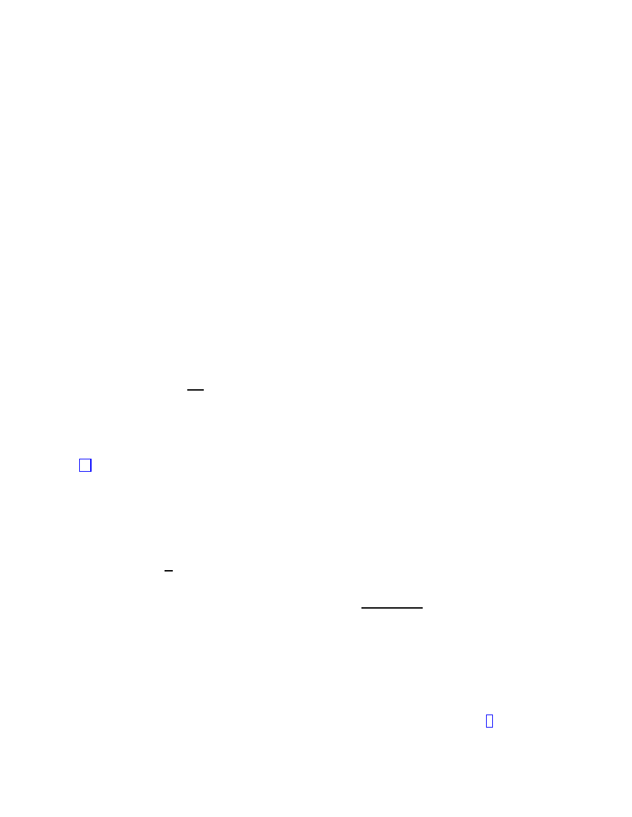
topologies (“genus”) (c.f. figure 2). This is allowed because in two (world-sheet) dimensions
one is allowed to discuss loop corrections in a way compatible with a (two-dimensional)
smooth manifold concept, in contrast to the point-particle one-dimensional case, where a
loop correction on the world-line (c.f. figure 2) cannot be described in a smooth way, given
that a particle loop does not constitute a manifold. The ‘somooth-manifold’ property of
quantum fluctuating world sheets is essential in analysing target-space quantum correc-
tions within a first-quantization framework, which cannot be done in the one-dimensional
particle case. Specifically, as we shall discuss later on, by considering the propagation of a
stringy extended object in a curved target space time manifold of higher-dimensionality (26
for Bosoninc or 10 for Superstrings), one will be able of arriving at consistency conditions
on the background geometry, which are, in turn, interpreted as equations of motion de-
rived from an effective low-energy action constituting the local field theory limit of strings.
Summation over genera will describe quantum fluctuations about classical ground states
of the strings described by world-sheet with the topology of the sphere (for closed strings)
or disc (for open strings).
To begin our discussion we first consider the propagation of a Bosonic string in a flat
target space of space-time dimensionality D, which will be determined dynamically below
by means of certain mathematical self-consistency conditions. From a first quantization
view point, such a propagation is described by considering the following world-sheet two-
dimensional action:
S
σ
=
−
T
2
Z
Σ
d
2
σ
√
γγ
αβ
η
M N
∂
α
X
M
∂
β
X
N
,
α, β = σ, τ
(1)
where γ
αβ
is the world-sheet metric, and X
M
(σ, τ ), D = 0, . . . D
− 1 denote a mapping
from the world-sheet Σ to a target space manifold of dimensionality D, of flat Minkowski
metric η
M N
, M, N = 0, . . . D
− 1. The world-sheet zero modes of the σ-model fields X
M
are therefore the spacetime coordinates, the 0 index indicating the (Minkowski) time. The
action (1) is related to the invariant world-sheet area, in direct extension of the point-
particle case, where a particle sweeps out a world line as it glides through space time,
and hence its action is proportional to a section of an invariant curve. The quantity
T is
the string tension, which from a target-space viewpoint is a dimensionful parameter with
dimensions of [length]
−2
. One then denotes
T =
1
2πα
0
(2)
3
Open String
σ
τ
topology of a disc
Types of Strings
Closed String
topology of a cylinder
Figure 1: Types of strings and the associated world-sheets swept as the string propagates
through a (higher-dimensional) target space time. In the closed-string case, which incorpo-
rates gravity, the point-like low-energy field theory limit is obtained by shrinking the size
of the external strings (at the tips of the cylinder) to zero, thereby obtaining the topology
of a punctured sphere
where α
0
is the Regge slope. This notation is a result of the original idea for which
string theory was invented, namely to explain hadron physics, and in particular the linear
dependence of the various hadron resonances of (toal) spin J vs Energy, the slope of which
was identified with the Regge slope
√
α
0
.
The dynamical world-sheet theory based on (1) is a constrained theory. This follows
from invariances, which are: (i) the reparametrizations of the world-sheet
(σ, τ )
→ (σ
0
, τ
0
) ,
(3)
playing the rˆole of general coordinate tranasformations in the two-dimensional world-sheet
manifold, and (ii) Weyl invariance, i.e. invariance of the theory under local conformal
rescalings of the metric :
γ
αβ
→ e
ϕ(σ,τ )
γ
αβ
,
(4)
where ϕ(σ, τ ) is a function of σ, τ . It should be noted that in two-dimensions the conformal
group is infinite dimensional, in contrast to its finite nature in all higher dimensions. It is
generated by the Virasoro algebra as we shall discuss later, and plays a crucial rˆole for the
quantum consistency of the theory (1), with important restrictions on the nature of the
target-space time manifold in which the string propagates.
4
NB: c.f. point−particle case:
+ ...
+
Looped world lines are not Manifolds though
are smooth
manifolds
World−sheets
Closed String Interactions
Open String Interactions
Figure 2: Quantum String Interactions are represented by higher-topologies on the asso-
ciated world-sheets. The two-dimensional nature of the string world-sheet, which makes
it a smooth manifold, should be contrasted with the point-particle world-line case, where
loops are not manifolds.
The symmetry under (i) and (ii) above allows one to fix the world-sheet metric into the
form:
γ
αβ
= e
ρ(σ,τ )
b
γ
αβ
(5)
where
b
γ
αβ
is a fiducial (fixed) metric on the world-sheet. As far as the two-dimensional
gravity (world-sheet) theory is concerned, the choice (5) is, in a sense, a “gauge choice”; this
is the reason why the ansatz is commonly called a conformal gauge. For most practical
purposes the metric
b
γ
αβ
is taken to be flat η
αβ
(plane). However formally this is not
quite correct in general, as it depends on the kind of string theory considered. For open
strings, whose classical (tree-level) propagation implies world-sheets with the topology of
a disc, the fiducial metric is that of a disc, i.e. a manifold with boundary. On the other
hand, for closed strings, whose classical (tree-level) propagation implies world-sheets with
the topology of a sphere (punctured), for point-like excitations, or cylinder, for stringy
excitations, the fiducial metric is taken to be that of a sphere or cylinder. In particular, in
the case of low-energy limit of strings, which implies that the external strings have been
shrunk to zero size, and hence they are punctures for all practical purposes, the spherical
5
topology of the fiducial geometry implies an Euler characteristic
χ = Euler characteristic = 2
− no. of holes − 2 × no. of handles =
2 =
1
4π
Z
b
Σ=S
(2)
q
b
γ
b
R
(2)
(6)
where
b
R
(2)
is the two-dimensional curvature. On the other hand, if one used naively a planar
fiducial metric, which as mentioned earlier, in many respect is sufficient, such topological
properties as (6), would be obscured. The importance of (6) will become obvious later
on, when we discuss quantum target-space string corrections (string loops), as opposed
to σ-model loops, i.e. world-sheet theory quantum corrections, which will be discussed
immediately below.
Under the gauge choice (5) the string equations (i.e. the equations of motion of the
fields X
M
) read:
∂
2
∂τ
2
−
∂
2
∂σ
2
!
X
M
= 0 ,
(wave equation)
(7)
and are supplemented with the constraint equations arising from vanishing variations
with respect to the world-sheet metric field γ
αβ
(which should be first varied and then be
constrained in the gauge (5) ):
δ
S
σ
δγ
αβ
= 0
(8)
The constraint (8) is nothing other than the vanishing of the stress-energy tensor T
αβ
of
the two-dimensional (world-sheet) field theory, defined as:
T
αβ
≡ −
2
T
√
γ
δ
S
σ
δγ
αβ
(9)
The above equations (7),(8) take their simplest form if one uses light-cone coordinates on
the world-sheet:
σ
±
= τ
± σ
(10)
Indeed, in this system of coordinates (8) becomes:
T
±±
= ∂
±
X
M
∂
±
X
N
η
M N
= 0,
T
+
−
= 0
(trace of stress tensor)
(11)
The vanishing of the trace of the stress tensor of the world-sheet theory implies an im-
portant symmetry, that of CONFORMAL INVARIANCE. The maintainance of this
classical symmetry at a quantum level is essential for the consistency of the theory, given
that above we have used this classical symmetry in order to make the choice (5). In the
next subsection we shall turn to a rather detailed discussion on the implications of the re-
quirement of conformal symmetry (which in two-dimensions implies an underlying infinite
dimensional (Virasoro) symmetry) at a quantum σ-model level.
6
Before doing this we simply mention that, in order to understand the existence of
an infinite number of conserved quantities, leading to an infinite-dimensional symmetry,
in the case of conformal symmetry in two space-time dimensions, it suffices to notice
that the conservation of the stress tensor T
αβ
, which is a consequence of two-dimensional
reparametrization invariance, in light-cone coordinates reads: ∂
−
T
++
+ ∂
+
T
−+
= 0. In
view of T
−+
= T
+
−
= 0, then, this implies ∂
−
T
++
= 0. If f (σ
+
) is an arbitrary function
of σ
+
, so that ∂
−
f = 0, then the current f T
++
is conserved, and hence the spatial integral
Q
f
≡
R
dσf (σ
+
)T
++
is a conserved charge. The arbitrariness of f implies therefore an
infinity of conserved charges. Clearly the argument above holds only in two dimensions.
In higher dimensions the conformal symmetry is finite dimensional.
2.2
Conformal Invariance and Critical Dimension of Strings
In this subsection we shall discuss the way by which conformal invariance is maintained at
a quantum σ-model level. First of all we should distinguish the quantum σ-model level,
which pertains to quantising the fields X
M
of the σ-model (in, say, a path integral) at
a fixed world-sheet topology, but integrating over world-sheet metrics (geometries), from
the quantum target-space level, at which one also summs up world-sheet topologies (string
loops).
The requirement of vanishing of the trace of the world-sheet stress tensor at a quantum
σ-model level implies important restrictions on the structure of the target space-time of
string theory. The first important restriction concerns the dimensionality of target space
time. There are various ways in which one can see this. In this lectures we shall follow the
covariant path integral quantization, which is most relevant for our purposes. For details
on other methods we refer the interested reader in the literature [1].
Consider the free field-theory world-sheet action, describing propagation of a free string
in a flat target space time (1).
S
σ
[γ, X] =
−
1
4πα
0
Z
Σ
d
2
σ∂
α
X
M
∂
β
X
N
η
M N
γ
αβ
√
γ
(12)
To quantize in a covariant path-integral way the above world-sheet action one considers
the partition function at a fixed world-sheet topology (genus):
Z =
Z
DγDXe
−iS
σ
[γ,X]
(13)
Formally one should analyticaly continue to a Euclidean world sheet and go back to the
Minkowskian signature world-sheet theory only at the end of the computations. This will
be understood in what follows.
We now concentrate on the integration over geometries on the world-sheet,
Dγ. This
integral is over three independent world-sheet metric components
: γ
++
(σ, τ ), γ
−−
(σ, τ ),
1
we work in the light-cone coordinate system, whose choice is allowed by postulating invariance under
general coordinate transformations of the two-dimensional quantum gravity theory. Notice that in two-
dimensions gravity is a renormalizable theory so the quantum path integral over world-sheet metrics is
rigorously well defined.
7
γ
+
−
(σ, τ ). An important rˆole is played by anomalies, i.e. the potential breakdown of
certain symmetries at a quantum world-sheet level, which result in the impossibility of
preserving all of the apparent classical symmetries of (13).
As we mentioned earlier there are three ‘gauge invariances’ of the action (1), two
reparametrizations of the world-sheet coordinates and a Weyl rescaling. Locally we can use
these symmetries to fix the gauge (5). For simplicity, in what follows, and given that we
shall work only at a fixed lowest topology on the world sheet, we shall consider the case of
flat fiducial metrics; however, the precise discussion on disc (spherical geometries) in case
of open (closed strings) should be kept in the back of the reader’s mind as the appropriate
procedure when one sums up genera.
In this case the covariant gauge reads:
γ
αβ
= e
ρ(σ,τ )
η
αβ
(14)
In light-cone coordinates then, the condition (14) implies:
0 = γ
++
= γ
−−
(15)
Under reparametrizations σ
±
→ σ
±
+ ξ
±
the world-sheet metric components in (15) trans-
form as:
δγ
++
= 2
∇
+
ξ
+
;
δγ
−−
= 2
∇
−
ξ
−
.
(16)
where
∇
α
denotes covariant world-sheet derivative, with respect to the metric γ. To
maintain (15) one should constraint the variations (16) to vanish.
Such conditions are implemented in the path integral (13) by means of insertion of the
identity:
1 =
Z
Dg(σ, τ )δ(γ
g
++
)δ(γ
g
−−
)det
δγ
g
++
δg
!
det
δγ
g
−−
δg
!
(17)
where
Dg denotes integration over the group G of reparametrizations of the string world-
sheet, and γ
g
denotes the world-sheet metric into which γ is transformed under the action
of G. The determinants det (. . .) appearing in (17) are due to the gauge fixing procedure
(14). We then have:
Z =
Z
Dg(σ, τ )
Z
DγDXe
−S
σ
[γ,X]
δ(γ
g
++
)δ(γ
g
−−
)det
δγ
g
++
δg
!
det
δγ
g
−−
δg
!
(18)
Reparametrization invariance implies that
S
σ
[γ, X] =
S
σ
[γ
g
, X], i.e. that the integrand
of the path integral depends on γ, g only through γ
g
. Making a change of variables from
γ, g to g and γ
0
≡ γ
g
, and discarding the
Dg intergation, which can be performed trivially
yielding an irrelevant constant proportionality (normalization) factor, one arrives at:
Z =
Z
Dγ
g
DXe
−S
σ
[γ
g
,X]
δ(γ
g
++
)δ(γ
g
−−
)det
δγ
g
++
δg
!
det
δγ
g
−−
δg
!
=
Z
Dγ
g
+
−
DXe
−S
σ
[γ
g
,X]
det
δγ
g
++
δg
!
|
γ
++
=0
det
δγ
g
−−
δg
!
|
γ
−−
=0
(19)
8
The integration over γ
g
+
−
is equivalent to an integration over the function ρ(σ, τ ) (c.f.
(14)). The determinants in the last expression can be expressed in terms of a set of
‘reparametrization ghost fields of Fadeev-Popov type’,
{c
±
, b
±±
}, of Grassmann statistics:
det
δγ
g
++
δg
!
|
γ
++
=0
=
Z
Dc
−
(σ, τ )
Db
−−
(σ, τ )e
−
1
π
R
Σ
d
2
σc
−
∇
+
b
−−
,
det
δγ
g
−−
δg
!
|
γ
−−
=0
=
Z
Dc
+
(σ, τ )
Db
++
(σ, τ )e
−
1
π
R
Σ
d
2
σc
+
∇
−
b
++
.
(20)
Hence one should have as a final result:
Z =
Z
Dρ(σ, τ )
Z
DX(σ, τ )Dc(σ, τ )Db(σ, τ )e
−S
total
[c,b,X]
,
(21)
where
S
total
=
S
σ
+
S
ghost
, with
S
ghost
=
1
2π
Z
d
2
σ
√
γγ
αβ
c
γ
∇
α
b
βγ
(22)
the action for the Fadeev-Popov ghost fields, written in a covariant form for completeness.
The c
γ
ghost field is a contravariant vector, while the ghost field b
βγ
is a symmetric traceless
tensor. Both fields b, c are of course anticommuting (Grassmann) variables, as mentioned
previously.
Quantization of the Ghost Sector.
We now proceed to discuss in some detail the quantization of the ghost sector of theory,
which has crucial implications for the dimensionality of the target space. From (22), the
stress tensor of the ghost sector T
ghost
αβ
≡ −
2π
√
γ
δ
S
ghost
δγ
αβ
(imposing the conformal gauge fixing
(14) at the end) reads:
T
ghost
αβ
=
1
2
c
γ
∇
(α
b
β)γ
+
∇
(α
c
γ
b
β)γ
− trace
(23)
In the light-cone coordinate system the only non-trivial components of T
ghost
are: T
ghost
++
, T
ghost
−−
:
T
ghost
++
=
1
2
c
+
∂
+
b
++
+ (∂
+
c
+
)b
++
,
T
ghost
−−
=
1
2
c
−
∂
−
b
−−
+ (∂
−
c
−
)b
−−
.
(24)
Canonical quantization of ghost fields imply the following anticommutation relation [1]:
{b
++
(σ, τ ), c
+
(σ
0
, τ )
} = 2πδ(σ − σ
0
) ,
{b
−−
(σ, τ ), c
−
(σ
0
, τ )
} = 2πδ(σ − σ
0
)
(25)
In what follows, for simplicity, we concentrate on the open string case. Comments on the
closed strings will be made where appropriate. The interested reader can find details on
9
this case in the literature [1]. In terms of ghost-field oscillation modes:
c
+
=
+
∞
X
−∞
c
n
e
−in(τ +σ)
,
c
−
=
+
∞
X
−∞
c
n
e
−in(τ −σ)
,
b
++
=
+
∞
X
−∞
b
n
e
−in(τ +σ)
,
b
−−
=
+
∞
X
−∞
b
n
e
−in(τ −σ)
,
(26)
one has the following anticommutation relations:
{c
n
, b
m
} = δ
m+n
,
{c
n
, c
m
} = {b
n
, b
m
} = 0
(27)
Using the Fourier modes of T
ghost
at τ = 0:
L
ghost
m
=
1
π
Z
π
−π
e
imσ
T
ghost
++
(28)
we have:
L
ghost
m
=
∞
X
n=
−∞
[m(J
− 1) − n]b
m+n
c
−n
(29)
where J is the conformal spin of the field b, with 1
− J that of the field c.
[NB1: For completeness we note that conformal dimensions are defined as follows (open
string case for definiteness): consider a local operator on the world sheet
F(σ, τ ). Set σ = 0
(or σ = π, the position of the boundaries of the open string) and study
F(0, τ ) ≡ F(τ ).
Then,
F(τ ) is defined to have conformal dimension (or ‘spin’) J if and only if, under an
arbitrary change of variables τ
→ τ
0
(τ ),
F(τ ) transforms as:
F
0
(τ
0
) =
dτ
dτ
0
!
J
F(τ )
(30)
The operators
L
ghost
m
in (28) are the generators of the infinite-dimensional Virasoro
algebra. The action of
L
m
on
F is:
[
L
m
,
F(τ )] = e
imτ
−i
d
dτ
+ mJ
!
F(τ )
(31)
or in terms of modes:
[
L
m
,
F] = [m(J − 1) − n]F
m+n
(32)
Note for completeness that for closed strings there is a second set of ghost Virasoro
generators.]
10
The Virasoro algebra of
L
ghost
m
is defined by the respective commutation relations:
h
L
ghost
m
,
L
ghost
n
i
= (m
− n)L
ghost
m+n
+
A(m)
ghost
δ
m+n
(33)
where the second term on the right-hand-side is a “conformal anomaly term”, indicating
the breakdown of conformal symmetry at a quantum σ-model level. It can be calculated
to be:
A(m)
ghost
=
1
12
[1
− 3(2J − 1)
2
]m
3
+
1
6
m
(34)
[NB2: The easiest way to evaluate the anomaly is to look at specific matrix elements, e.g.
:
A(1)
ghost
=
h0|
h
L
ghost
1
,
L
ghost
−1
i
|0i. ]
The ghost field b has J = 2, so that the anomaly in the ghost sector is:
A(m)
ghost
=
1
6
(m
− 13m
3
)
(35)
Similar quantization conditions characterize the matter sector of the σ-model (1), per-
taining to the fields/coordinates X
M
. We shall not do the analysis here. The interested
reader is referred for details and results in the literature [1]. Adding such ghost and matter
contributions, the total conformal anomaly (for a D-dimensional target space time) is [1]
is found as follows: first we note that the Virasoro generators corresponding to
S
total
=
S
σ
+
S
ghost
, are the Fourier modes
L
m
=
1
π
R
π
−π
dσe
imσ
T
total
++
, where T
total
++
=
−
2π
γ
δ
S
total
δγ
++
|
γ
++
=0
,
and
L
m
=
L
matter
m
+
L
ghost
m
− aδ
m
, and we have shifted the definition of
L
0
(related to
the Hamiltonian of the string) so that the zeroth-order Virasoro constraint is
L
0
= 0.
Then, following similar mode expansions for the matter sector, as those of the ghost sector
outlined above, one arrives at the total conformal anomaly:
A(m) =
D
12
(m
3
− m) +
1
6
(m
− m
3
) + 2am
(36)
where D is the target-space dimensionality (corresponding to the contributions from D
σ-model “mater” fields X
M
). From (36) one observes that the anomaly VANISHES, and
thus conformal world-sheet symmetry is a good symmetry at a quantum σ-model level, as
required for mathematical self-consistency of the theory, if and only if:
D
c
= 26
(Bosonic String) ,
a = 1
(37)
For fermionic (supersymmetric strings (cf below)) the critical space-time dimension is
D
c
= 10.
2.3
Some Hints towards Supersymmetric Strings
So far we have examined Bosonic strings. Supersymmetric strings are more relevant for
particle phenomenology, because as we shall discuss now, do not suffer from vacuum in-
stabilities like the bosonic counterparts, which are known to contain in their spectrum
11
tachyons (negative mass squared modes). Moreover such theories are capable of incorpo-
rating fermionic target-space backgrounds.
There are two ways to include fermionic backgrounds in a σ-model string theory, and
thus to achieve target-space supersymmetry:
(1) The first one is to supersymemtrize the world-sheet theory by introducing fermionic
partners ψ
M
(σ, τ ) to the X
M
(σ, τ ) fields. There are two kinds of fermions that can be
introduced, depending on their boundary conditions (b.c.) on a circle, so that the world-
sheet fermion action is invariant under periodic identification on a cylinder σ
→ σ + 2π:
ψ
M
(σ = 0) =
−ψ
M
(σ = 2π) antiperiodic b.c. : Neveu
− Schwarz (NS),
ψ
M
(σ = 0) = ψ
M
(σ = 2π)
periodic b.c. : Ramond (R)
(38)
As a result of the presence of these extra degrees of freedom, world-sheet supersymmetry
leads to a reduction of the critical target-space dimension, for which the conformal anomaly
is absent, from 26 to 10 (i.e. the critical target-space dimensionality of a superstring is
10).
A world-sheet supersymmetric σ-model does not have manifest supersymmetry in target
space; the latter is obtained after appropriate spectrum projection (Goddard, Scherk and
Olive [1]).
(2) The second way of introducing fermionic backgrounds in string theory is to have bosonic
world sheets but with manifest target-space Supersymmetry (Green and Schwarz).
The two methods are equivalent, as far as target-space Supersymmetry is concerned.
Features of Supersymmetric Strings.
• (i) The tachyonic instabilities in the spectrum, which plagued the Bosonic string, are
absent in the supersymmetric string case. This stability of the superstring vacuum
is one of the most important arguments in favour of (target-space) supersymmetry
from the point of view of string theory.
• (ii) From a world-sheet viewpoint, in the Neveu-Schwarz-Ramond formulation of
fermionic strings, the world-sheet action becomes a curved two-dimensional locally
supersymmetric theory (world-sheet supergravity theory).
• (iii) Target Supersymmetry is broken in general when one considers strings at fi-
nite temperatures, obtained upon appropriate compactification of the target-space
coordinate. In general, however, the breaking of target supersymmetry at zero tem-
perature, so as to make contact with realistic phenomenologies, is an open issue at
present, despite considerable effort and the existence of many scenaria.
2.4
Kaluza-Klein Compactification
The fact that the target space-time dimensionality of strings turns out to be higher than
four implies the need for compactification of the extra dimensions.
12

Compactification means that the ground state of string theory has the form:
M
(4)
⊗ K
(39)
where
M
(4)
is a four-dimensional non-compact manifold (assumed Minkowski, but in fact it
can be any other space time encountered in four-dimensional general relativity, priovided
it satisfies certain consistency conditions to be discussed below), and
K is a compact
manifold, six dimensional in the case of superstrings, or 22 dimensional in the case of
(unstable) Bosonic strings.
In “old” (conventional) string theory [1], the “size” of the extra dimensions is assumed
Planckian, something which in the modern brane version is not necessarily true. For our
purposes in these Lectures we shall restrict ourselves to the “old” string theory approach
to compactification.
Consider a 26-(or 10-)dimensional metric on
M
(4)
⊗ K, g
M N
, and let g
µν
∈ M
(4)
, and
g
ij
∈ K.
From a four-dimensional point of view g
ij
appear as massless spin-one particles, i.e.
massless gauge bosons. This is the central point of Kaluza-Klein (KK) approach. Such
particles appear if a suitable subgroup of the underlying ten-dimensional general covariance
is left unbroken under compactification to
M
(4)
⊗ K. Let us see this in some detail.
Consider a general coordinate transformation on the manifold
K:
y
k
→ y
k
+ V
k
(y
j
)
(40)
where is a small parameter, and V
k
a vector field. In the passive frame, the corresponding
change of the metric tensor g
ij
is:
δg
ij
= (
∇
i
V
j
+
∇
j
V
i
)
(41)
where
∇
i
is the gravitational covariant derivative. The metrc on
K is therefore invariant
if V
k
obeys a Killing-vector equation:
∇
i
V
j
+
∇
j
V
i
= 0
(42)
Thus, the coordinate transformation (40), generated by the Killing vector V
k
, is a symme-
try of any generally-covariant equation for the metric of
K. More generally, if one studies
an equation involving a coupled system of the metric with some other matter fields (e.g.
gauge fields etc.), then one obtains a symmetry if V
k
can be combined with a suitable
transformation of the matter fields that leaves their expectation values invariant.
Consider the case in which one has several Killing vector fields V
i
a
, a = 1, . . . N , gener-
ating a Lie algebra
H of some kind:
h
V
i
a
∂
i
, V
j
b
∂
j
i
= f
abc
V
k
c
∂
k
(43)
where f
abc
are the corresponding structure constants of the Lie algebra that generates a
symmetry group
H on K.
13
Consider the transformation
x
µ
, y
k
→
x
µ
, y
k
+
X
a
a
V
k
a
!
(44)
In the general case one may consider non-constant
a
=
a
(x
µ
) on
M
(4)
.
At long wavelengths, which are of interest to any low-energy observer, only massless
modes are important. Therefore, the transformation (44) will be a symmetry of the the-
ory compactified on
M
(4)
⊗ K. From the point of view of the four-dimensional effective
low-energy theory the transformations (44) will look like
M
(4)
-dependent local gauge trans-
formations with gauge group
H. The effective four-dimensional theory will therefore have
massless gauge bosons given by the ansatz:
g
µj
=
X
a
A
a
µ
(x
ν
)V
ja
(y
k
)
(45)
where A
a
µ
(x
ν
) are the massless gauge fields that appear in
M
(4)
. This follows from the
fact that under (44), the fields A
a
µ
in (45) transform as ordinary gauge fieldds: δA
a
µ
=
∂
µ
a
+ f
abc
b
A
µc
.
An interesting question arises at this point as to what symmetry groups can arise via
KK compactification. This is equivalent to asking what symmetry groups an n-dimensional
manifold can have.
We consider for completeness the case where
K has dimension n, which is kept general
at this point. The most general answer to the above question is complicated. An interesting
question, of phenomenological interest, is for which n one can get the standard model group
SU (3)
⊗ SU(2) ⊗ U(1). It can be shown [1] that this happens for n = 7 which it is not
the case of string theory (superstrings), since in that case n = 6. This is what put off
people’s interest in the traditional KK compactification, which was instead replaced by
the heterortic string construction, which we shall not analyse here [1]. On the other hand,
it should be mentioned that in the modern version of string theory, involving branes, KK
modes play an important rˆole again. For more details we refer the reader to the lectures
on brane theory in this School.
2.5
Strings in Background Fields
So far we have dealt with flat Minkowski target space times. In general strings may be
formulated in curved space times, and, in general, in the presence of non-trivial back-
ground fields. In this case conformal invariance conditions of the underlying σ-model
theory become equivalent, as we shall discuss below, to equations of motion of the various
target-space background fields.
The lowest lying energy multiplet in superstring theory consists (in its bosonic part) of
massless states of gravitons g
M N
(spin two traceless and symmetric tensor field), dilaton
Φ (scalar, spin 0) and antisymmetric tensor B
M N
field
. Target space supersymmetry, of
2
In the Bosonic states the lowest lying energy state (vacuum) is tachyonic, and the above multiplet
occurs at the next level.
14
course, implies the existence of the supersymmetric (fermionic) partners of the states in
this multiplet. In this section we shall discuss the formalism, and its physical consequences,
for string propagation in the bosonic part of the massless superstring multiplet, starting
from graviton backgrounds, which are discussed next.
2.5.1
Formulation of Strings in Curved Space times-Graviton Backgrounds
The corresponding σ-model action, describing the propagation of a string in a space time
with metric g
M N
reads:
S
σ
=
1
4πα
0
Z
Σ
d
2
σ
√
γγ
αβ
g
M N
(X
P
(σ, τ ))∂
α
X
M
∂
β
X
N
,
α, β = σ, τ
(46)
One expands around a flat target space time g
M N
= η
M N
+ h
M N
(X). For
|h
M N
(X)
| 1
one may expand in Fourier series:
h
M N
(X)
=
Z
d
D
k
(2π)
D
e
ik
M
X
M
˜h
M N
(k)
(47)
in which case the σ-model action becomes schematically:
S
σ
= S
∗
+
1
4πα
0
Z
Σ
d
2
σ
√
γγ
αβ
∂
α
X
M
∂
β
X
N
Z
d
D
k
(2π)
D
e
ik
M
X
M
˜h
M N
(k)
≡
S
∗
+ g
i
Z
Σ
d
2
σV
i
(48)
where S
∗
is the flat space-time action (1), and one has the correspondence g
i
←→ ˜h
M N
(k),
V
i
←→
√
γγ
αβ
∂
α
X
M
∂
β
X
N
e
ik
P
X
P
, and
P
i
←→
R
d
D
k
(2π)
D
.
It should be stressed that implementing a Fourier expansion necessitates an expansion
in the neighborhood of the Minkowski space time, so as to be able to define plane waves
appropriately. For generic space times one may consider an expansion about an appropriate
conformal (fixed point) σ-model action S
∗
, as in the last line of the right-hand-side of (48),
but in this case the set of background fields/σ-model couplings
{g
i
} is found as follows:
consider g
M N
= g
∗
M N
+ h
M N
(X), where g
∗
M N
a conformal (fixed-point) non-flat metric, and
h
M N
(X) an expansion around it. Then,
S =
1
4πα
0
Z
Σ
d
2
σ∂
α
X
M
∂
β
X
N
g
M N
γ
αβ
√
γ =
S
∗
+
1
4πα
0
Z
Σ
d
2
σh
M N
(X)∂
α
X
M
∂
β
X
N
γ
αβ
√
γ =
S
∗
+
1
4πα
0
Z
Σ
d
2
σ
Z
d
D
y
q
g
∗
(y)δ
(D)
y
M
− X
M
(σ, τ )
·
h
M N
(y)∂
α
X
M
∂
β
X
N
γ
αβ
√
γ
≡
S
∗
+ g
i
Z
σ
d
2
σV
i
(49)
15
where g
i
←→ {h
M N
(y)
}, V
i
←→ δ
(D)
y
M
− X
M
(σ, τ )
∂
α
X
M
∂
β
X
N
γ
αβ
√
γ, and
P
i
←→
R
d
D
y
q
g
∗
(y). As the reader must have noticed, for general backgrounds one pulls out the
world-sheet zero mode of X
M
appropriately, which defines the target-space coordinates, and
integrates over it, thereby determining the (infinite dimensional) set of σ-model couplings.
2.5.2
Other Backgrounds
We continue our discussion on formulating string propagation in non-trivial backgrounds,
in the first-quantized formalism, by studying next antisymmetric tensor and dilatons.
Antisymmetric Tensor Background
The antisymmetric tensor backgrounds B
M N
are spin one, antisymmetric tensor fields
B
M N
=
−B
N M
. There is an Abelian gauge symmery which characterizes the corresponding
scattering amplitudes (with antisymmetric tensors as external particles),
B
M N
→ B
M N
+ ∂
[M
Λ
N ]
(50)
which implies that the corresponding low-energy effective action, which reproduces the
scattering amplitudes, will depend only through the field strength of B
M N
: H
M N P
=
∂
[M
B
N P ]
.
In a σ-model action the pertinent deformation has the form:
1
4πα
0
Z
Σ
d
2
σB
M N
V
(B)M N
=
1
4πα
0
Z
Σ
d
2
σB
M N
αβ
∂
α
X
M
∂
β
X
N
(51)
where
αβ
is the contravariant antisymmetric symbol.
[NB3:due to its presence there is no explicit √γ factor in (51), as this is incorporated in
the contravariant -symbol. ]
Dilaton Backgrounds and the String Coupling
The dilaton Φ(X) is a spin-0 mode of the massless superstring multiplet, which in a
σ-model framework couples to the world-sheet scalar curvature R
(2)
(στ ):
S
σ
=
1
4πα
0
Z
Σ
d
2
σ
√
γγ
αβ
∂
α
X
M
∂
β
X
M
+
1
4π
Z
Σ
d
2
σ
√
γΦ(X)R
(2)
(σ, τ )
(52)
Notice that in the dilaton term there is no α
0
factor, which mplies that in a (perturbative)
series expansion in terms of α
0
the dilaton couplings are of higher order as compared with
the graviton and antisymmetric tensor backgrounds.
An important rˆole of the dilaton is that it determines (via its vacuum expectation value)
the strength of the string interactions, the string coupling:
String Coupling g
s
= e
hΦi
(53)
where < . . . >=
R
DXe
S
σ
is computed with respect to the string path integral for the
σ-model propgating in the background under consideration.
16
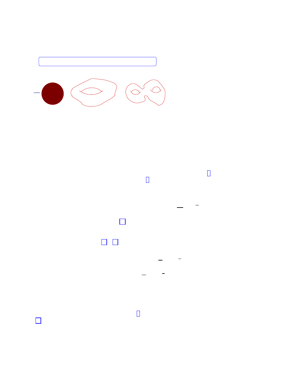
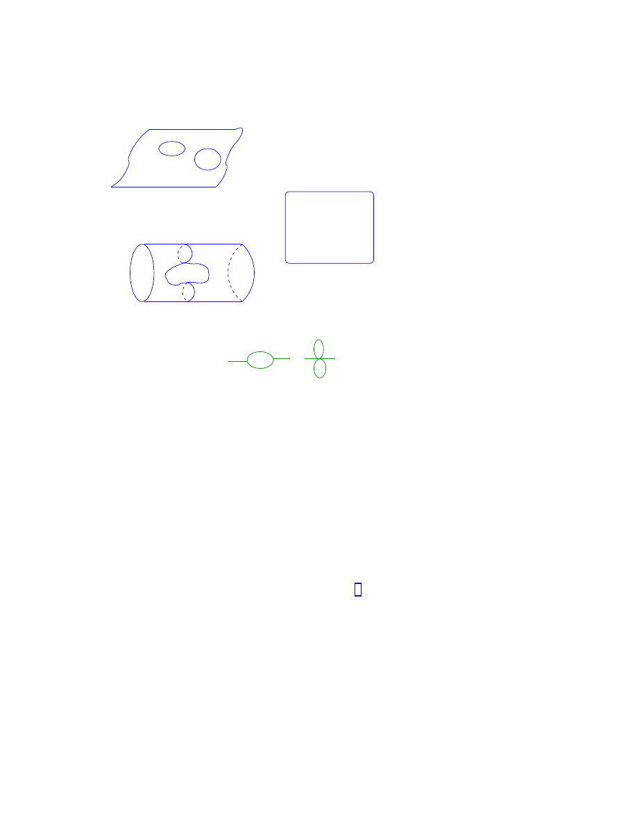
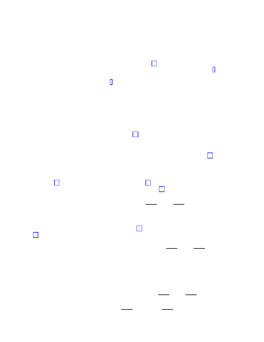
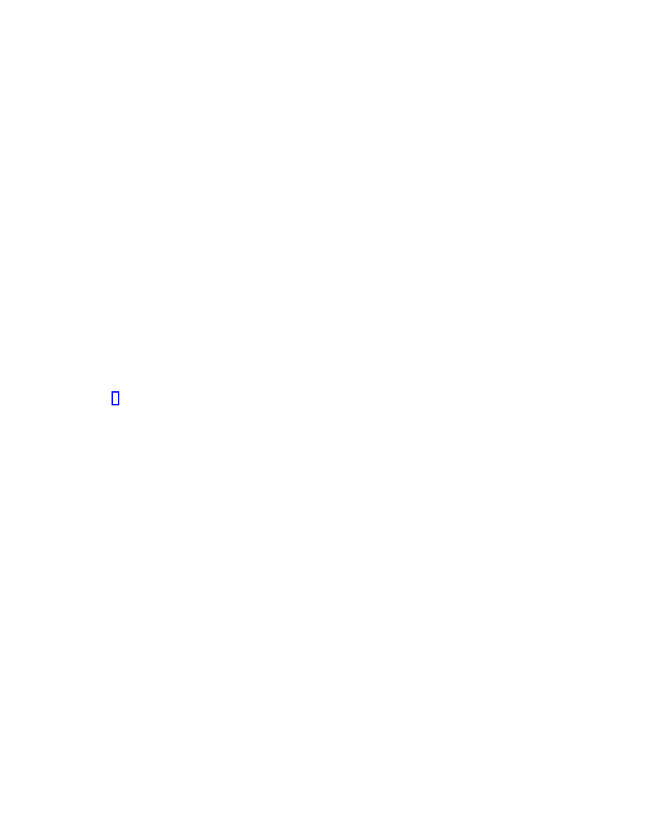
g
2
s
,
,
2d sphere
Torus
Higher genus
Riemann surface
s
g
2
1
String Coupling as String Loop counting parameter
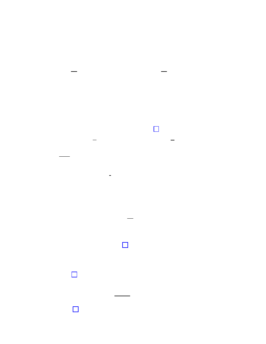
Figure 3: The string coupling g
s
= e
<Φ>
as a string-loop counting parameter. The loop
expansion parameter is g
−χ
s
, where χ is the Euler characteristic of the manifold. For the
sphere one has χ
S
= 2, for a torus (flat) χ
T
= 0 etc.. Such weights are depicted explicitly
in the figure
The string coupling is a string-loop counting parameter (c.f. figure 3). This can be
seen easily by first recalling the index theorem (6) that connects a geometrical world-sheet
quantity like the curvature R
(2)
to a topological quantity, the Euler characteristic χ, which
counts the genus of the surface:
χ = 2
− no. of holes − 2 × no. of handles =
1
4π
Z
Σ
√
γR
(2)
(54)
Consider the σ-model deformation (52) and split the dilaton into a classical (world-sheet
coordinate independent) part < Φ > and a quantum part
ϕ
≡: Φ :, where : . . . : denotes appropriate normal ordering of the corresponding operators:
Φ =< Φ > +ϕ(σ, τ ). Using (54),(53), we can then write for the σ-model partition function
summed over surfaces of genus χ:
Z =
X
χ
Z
DXe
−S
rest
−χ<Φ>−
1
4π
R
Σ
d
2
σ√γϕR
(2)
=
X
χ
g
−χ
s
Z
DXe
−S
rest
−
1
4π
R
Σ
d
2
σ√γϕR
(2)
(55)
where S
rest
denotes a σ-model action involving the rest of the background deformations
except the dilaton. For a sphere, χ = 2 (for a disc (open strings) χ = 1), for torus (one
string loop) χ = 0, etc. By normalizing the higher-loop contributions to the sphere, then,
one gets the string-loop series depicted in 3, with a clear interpretation of the quantity
(53) as a string-loop counting parameter.
17

2.6
Conformal Invariance and Background Fields
The presence of σ-model “deformations” g
i
R
Σ
V
i
imply in general deviations from conformal
invariance on the world sheet. To ensure conformal invariance we must impose certain
conditions on the couplings g
i
. Such conditions, and their implications will be studied
in this section. As we shall see, the conformal invariance conditions are equivalent to
equations of motion for the target-space background g
i
which are derived from a target-
space string effective action. This action constitutes the low-energy (field-theory) limit
of strings and will be the main topic of these lectures. String cosmology, which we shall
discuss in the second and third lectures, will be based on such string effective actions.
To start with, let us consider a deformed σ-model action
S = S
∗
+ g
i
Z
Σ
d
2
σV
i
(56)
which, as we have discussed above, describes propagation (in a first quantized formalism)
of a string in backgrounds
{g
i
} = {g
M N
, Φ, B
M N
, . . .
}.
The partition function of the deformed string may be expanded in an (infinite) series
in powers of g
i
(assumed weak):
Z[g] =
Z
DρDXe
−S
∗
−g
i
R
Σ
d
2
σV
i
=
X
i
i
Z
Σ
. . .
Z
Σ
hV
i
1
. . . V
i
N
i
∗
g
i
1
. . . g
i
N
d
2
σ
1
. . . d
2
σ
N
(57)
where
h. . .i
∗
=
R
DρDXe
−S
∗
. We work in the conformal gauge (5), and thus the mode ρ
is whatever is left from the integration over world-sheet geometries. In conformal (‘criti-
cal’) string theory the quantities
hV
i
1
. . . V
i
N
i
∗
are nothing other than the string scattering
amplitudes (defining the on-shell S-matrix elements) for the modes corresponding to
{g
i
}.
It must be stressed that critical string theory is by definition a theory of the S-matrix,
and hence this imposes a severe restriction on the appropriate backgrounds. Namely, as
we shall discuss in Lecture 3, appropriate string backgrounds are those which can admit
asymptotic states, and hence well-defined on-shell S-matrix elements
.
As a two-dimensional quantum field theory, the model (56) suffers from world-sheet
ultraviolet (short-distance) divergences, which should not be confused with target-space
ultraviolet infinities. Such world-sheet infinities arise from short-distance regions
lim
σ
1
→σ
2
hV
i
1
(σ
1
) . . . V
i
2
(σ
2
)V
i
3
(σ
3
) . . . V
i
N
(σ
N
)
i
∗
, and they are responsible for the breaking
of the conformal invariance at a quantum level, because they require regularization, and
regularisation implies the existence of a length (short-ditance) cutoff. The presence of such
length cutoff regulators break the local (and global) scale invariance in general. Below we
shall seek conditions under which the conformal invariance is restored.
3
Eternally accelerating string Universe backgrounds, for instance, which will be the topic of disucssion
in the last part of our lectures, are incompatible with critical string theory, precisely because of this,
namely in such backgrounds one cannot define appropriate asymptotic pure quantum states. We shall
discuss how such problems may be overcome in the last part of the lectures.
18
To this end, we first observe that, according to the general case of renormalizable
quantum field theories, one of which is the σ-model two-dimensional theory (56), such
infinities may be absorbed in a renormalization of the string couplings. To this end,
one adds appropriate counterterms in the σ-model action, which have the same form as
the original (bare) deformations, but they are renormalization-group scale dependendent.
Therefore their effect is to ‘renormalise’ the couplings g
i
→ g
R
i
(lnµ), where µ is a world-
sheet renormalization group scale.
The scale defines the β-functions of the theory:
β
i
≡
dg
i
R
dlnµ
=
X
i
n
C
i
i
1
...i
n
g
i
1
R
. . . g
i
n
R
(58)
One can show in general that the (2d-gravitational) trace Θ
≡ T
αβ
γ
αβ
of the world-sheet
stress tensor in such a renormalized theory can be expressed as:
hΘi = c R
(2)
+ β
i
hV
i
i
(59)
where c is the conformal anomaly of the world-sheet theory, and R
(2)
is the world-sheet
curvature. In the case of strings living in their critical dimension, the total conformal
anomaly c, when Fadeev-Popov contributions are taken into account vanishes, as we have
seen in the beginning of this lecture. Thus to ensure conformal invariance in the presence
of background fields g
i
, i.e.
hΘi = 0 one must impose
β
i
= 0
(60)
These are the conformal invariance conditions, which in view of (58) imply restrictions on
the background fields g
i
.
A few comments are important at this point before we embark on a discussion on the
physical implications for the target-space theory of the conditions (60). The comments
concern the geometry of the ‘space of coupling constants
{g
i
}’, so called moduli space of
strings, or string theory space. As discussed first by Zamolodchikov [3], such a space is a
metric space, with the metric being provided by the two-point functions of vertex operators
V
i
in the deformed theory,
G
ij
= z
2
¯
z
2
hV
i
(z, ¯
z)V
i
(0, 0)
i
g
(61)
where z, ¯
z are complex coordinate of a Euclidean world sheet, which is necessary for con-
vergence of our path integral formalism. The notation
h. . .i
g
denotes path integral with
respect to the deformed σ-model action (56) in the background
{g
i
}. The metric (61) acts
as a raising and lowering indices operator in g
i
-space.
An important property of the stringy σ-model β-functions is the fact that the ‘covari-
ant’ β-functions, defined as β
i
=
G
ij
β
j
, when expanded in powers of g
i
have coefficients
completely symmetric under permutation of their indices, i.e.
β
i
=
G
ij
β
j
=
X
i
n
c
i
1
i
2
...i
n
g
i
2
. . . g
i
n
(62)
19
with c
i
1
i
2
...i
n
totally symmetric in the indices i
j
. This can be proven by using specific
properties of the world-sheet renormalization group [4]. Such totally symmetric coefficients
are associated with dual string scattering amplitudes, as we shall demonstrate explicitly
later on.
What (62) implies is a gradient flow property of the stringy β-functions, namely that
δC[g]
δg
i
=
G
ij
β
j
(63)
where C[g] is a target-space space-time integrated functional of the fields g
i
(y).
Notice that the conformal invariance conditions (58) are then equivalent to equations
of motion obtained from this functional C[g], which thus plays the rˆole of a target-space
effective action functional for the low-energy dynamics of string theory.
An important note should be made at this point, concerning the rˆole of target-space
diffeomorphism invariance in stringy σ-models. As a result of this invariance, which is
a crucial target-space symmetry, that makes contact with general relativity in the target
manifold, the conformal invariance conditions (58) in the case of strings are slightly mod-
ified by terms which express precisely the change of the background couplings g
i
under
general coordinate diffeomorphisms in target space δg
i
:
b
β
i
= β
i
+ δg
i
= 0
(64)
in other words conformal invariance in σ-models implies the vanishing of the modified β-
functions, i.e. it is valid up to general coordinate diffeomorphism terms. This modification
plays an important rˆole in ensuring the compatibility of the solutions with general coor-
dinate invariance of the target manifold. The modified β-functions
b
β
i
are known in the
string literature as Weyl anomaly coefficients [1]. In fact, for the stringy σ-model case,
they appear in the expression (59), in place of the ordinary β
i
.
2.7
General Methods for Computing β-functions
In general there are two kinds of perturbative expansions in σ-model theory.
• (I) Weak Coupling g
i
-expansion: in which one assumes weak deformations of
conformal σ-model actions, with g
i
small enough so as a perturbative series expansion
in powers of g
i
suffices. Usually in this method one deals with Fourier modes (cf
below) of background deformations, and hence the results are available in target-
momentum space; this is appropriate when one considers scattering amplitudes of
strings.
• (II) α
0
-Regge slope expansion: in which one considers an expansion of the parti-
tion function and correlation functions of σ-models in powers of α
0
. Given that the
Regge slope has dimensions of [length]
2
, such expansions imply (in Fourier space)
appropriate derivative expansions of the string effective actions. It is the second ex-
pansion that will be directly relevant for our Cosmological considerations. The Regge
slope expansion preserves general covariance explicitly.
20
It should be stressed that physically the two methods of expansion are completely
equivalent. Formally though, as we have mentioned, the various methods may have advan-
tages and disadvantages, compared to each other, dependending on the physical problem at
hand. For instance when one deals with weak fields, then the first method seems appropri-
ate. In field theory limit of strings, on the other hand, where by definition we are interested
in low-energies compared with the string (Planckian
∼ 10
19
GeV) scale, then the second
expansion is more relevant. Moreover it is this method that allows configuration-space
general covariant expressions for the effective action in arbitrary space-time backgrounds,
in which momentum space may not always be a well-defined concept.
Before we turn into an explicit discussion on string effective actions we consider it
as instructive to discuss, thorugh a simple but quite generic example, the connection of
conformal invariance conditions to string scattering amplitudes through the first method.
2.7.1
String Amplitudes and World-Sheet Renormalization Group
A generic structure of a renormalization-group β-function in powers of the renormalized
couplings g
i
(t) is:
β
i
=
dg
i
dt
= y
i
g
i
+ α
i
jk
g
j
g
k
+ γ
i
jk`
g
j
g
k
g
`
+ . . . ,
t = lnµ
(65)
where y
i
are the anomalous dimensions, and no summation over the index i is implied in
the first term. Summation over repeated indices in the other terms is implied as usual.
The bare cuplings are the ones for which t = 0, g
i
(0)
≡ g
i
0
. The perturbative solution of
(65), order by order in a power series in g
i
, is:
• First Order:
g
i
(t) = e
y
i
t
g
i
(0).
(66)
• Second Order
g
i
(t) = e
y
i
t
g
i
(0) + δ
i
jk
g
j
(0)g
k
(0) ,
(67)
with ˙δ
i
jk
≡
d
dt
δ
i
jk
= α
i
jk
e
y
j
t
e
y
k
t
+ y
i
δ
i
jk
;
δ
i
jk
(0) = 0, from which :
δ
i
jk
(t) =
e
(y
j
+y
k
)t
− e
y
i
t
α
i
jk
y
j
+ y
k
− y
i
(68)
and so on. Notice from the expression for the second order terms the resemblance of the
anomalous-dimension denominators with “energy denominators” in scattering amplitudes.
As we shall discuss below this is not a coincidence; it is a highly non-trivial property of
string renormalization group to have a close connection with string scattering amplitudes.
We shall explain this through a simplified but quite instructive, and in many respects
generic, excample, that of an open Bosonic string in a tachyonic background [5].
Open Strings in Tachyonic Backgrounds: Weak Field Expansion
21
The σ-model action, for an open string propagating in flat space time in a tachyon
background T (X), is:
S
open
=
1
4π
Z
dxdy η
αβ
∂
α
X
M
∂
β
X
N
η
M N
+
Z
+
∞
−∞
dx
a
Z
d
26
k ˜
T (k)e
ik
M
X
M
(69)
where we work in units of α
0
= 1, and a is a length scale, which will play the rˆole of a
short-distance cut-off scale. Notice that the world-sheet is taken here to be the upper half
plane for simplicity. The open string interactions occur at the world-sheet boundary, and
this is expressed by the fact that the tachyonic background term is over the real x axis.
We apply the background field method for quantization, according to which we split the
fields X
M
= X
M
0
+ξ
M
, where X
M
0
satisfies the classical equations of motion, and varies slow
with respect to the cut-off scale a. The effective action is defined as S
eff
[X
0
] =
−lnW [X
0
],
where W [X
0
] is the partition function of the σ-model (69):
W [X
0
] =
Z
Dξe
−
1
4π
R
y>0
dxdy η
αβ
∂
α
X
M
∂
β
X
N
η
M N
e
−
R
+
∞
−∞
dx
a
R
dk ˜
T (k)e
ik
·X0
e
ik
·ξ
(70)
where dk
≡
d
26
k
(2π)
26
is the target momentum space integration. Using the free-feld contrac-
tion, with the scale a as a short-distance regulator,
hξ(x
1
)ξ( 2)
i
∗
=
−2ln (|x
1
− x
2
| + a)
(71)
where * denotes free-field σ-model action (in flat target space), and expanding the σ-model
partition function in powers of ˜
T (k), we obtain the folowing results, order by order in the
weak-field (tachyon) expansion:
Linear order in ˜
T (k): to this order, the partition function W [X
0
] becomes:
W [X
0
]
(1)
=
−
Z
+
∞
−∞
dx
a
Z
dk ˜
T (k)e
ik
·X
0
he
ik
·ξ
i
∗
=
−
Z
+
∞
−∞
dx
Z
dka
k
2
−1
˜
T (k)e
ik
·X
0
(72)
where we used the free-field contraction (71). The scale a-dependence may be absorbed in
a renormalization of the coupling ˜
T (k) :
˜
T
R
(k)
≡ a
k
2
−1
˜
T (k)
(73)
Comparing with (66), we observe that one may identify a = e
−t
, t the renormalization-
group (RG) scale, from which one obtains the β-function:
β
T
(k) =
−
d ˜
T
R
(k)
dlna
=
−(k
2
− 1) ˜
T
R
(k)
(74)
Comparison with (65), then, indicates that the anomalous dimension is k
2
− 1.
22
The conformal invariance conditions (60) amount to the vanishing of the β-function,
which thus turns out to be equivalent to the on-shell condition for tachyons:
− (k
2
− 1) ˜
T
R
(k) = 0
→ k
2
= 1
(75)
This is the first important indication that the conformal invariance conditions of the stringy
σ-model imply important restrictions for the dynamics of the background over which it
propagates.
Less trivial consequences for the background become apparent if one examines the next
order in the expansion in powers of ˜
T (k).
Quadratic Order in ˜
T (k): to this order the partition function W [X
0
] reads:
W [X
0
]
(2)
=
Z
+
∞
−∞
dx
1
a
Z
+
∞
−∞
dx
2
a
Z
dk
1
˜
T (k
1
)
Z
dk
2
˜
T (k
2
)
·
e
ik
1
·X
0
(x
1
)+ik
2
·X
0
(x
2
)
he
ik
1
·ξ(x
1
)+ik
2
·ξ(x
2
)
i
∗
(76)
Since X
0
varies slowly, one may expands a l´a Taylor: X
0
(x
2
) = X
0
(x
1
) + (x
2
− x
1
)X
0
0
(x
1
) +
. . .
' X
0
(x
1
) to a good approximation.
Implementing the free-field contraction (71), and performing straightforward algebraic
manipulations, we arrive at integrals of the form:
a
k
2
1
+k
2
2
−2
Z
x
1
−∞
dx
2
(x
1
− x
2
− a)
2k
1
·k
2
=
−a
(k
1
+k
2
)
2
−1
1
2k
1
· k
2
(77)
The integral converges for
2k
1
· k
2
− 1 < 0
(78)
Absorbing the scale dependence in renormalized tachyons, as before, one obtains to second
order:
˜
T
R
(k) = a
k
2
−1
˜
T
R
(k) +
Z
dk
1
Z
dk
2
˜
T
R
(k
1
) ˜
T
R
(k
2
)
2k
1
· k
2
+ 1
δ
(26)
(k
1
+ k
2
− k)
!
(79)
Comparing (67), (68) with (79), we observe that we are missing the term a
−y
1
−y
2
=
a
k
2
1
+k
2
2
−2
. To the order we are working, this discrepancy can be justified as folows: re-
moving the cut-off, i.e. going to a non-trivial fixed point t
→ ∞, and taking into account
the convergence region (78), which implies y
1
+ y
2
< y, with y = k
2
− 1 the anomalous
dimension, we observe that in the regime t
→ ∞ the missing term is negligible compared
with the one which is present, and thus the above computation is consistent with the
generic renormalization group analysis, near a non-trivial fixed point. One then defines
the β-functions of the theory, away from a fixed point (in the entire (target) momentum
space) by analytic continuation.
Comparing the above results with (67),(68) we then find that to second order:
2k
1
· k
2
+ 1 = y
1
+ y
2
− y,
(y
i
= 1
− k
2
i
),
α
k
k
1
k
2
=
−δ
(26)
(k
1
+ k
2
− k)
(80)
23
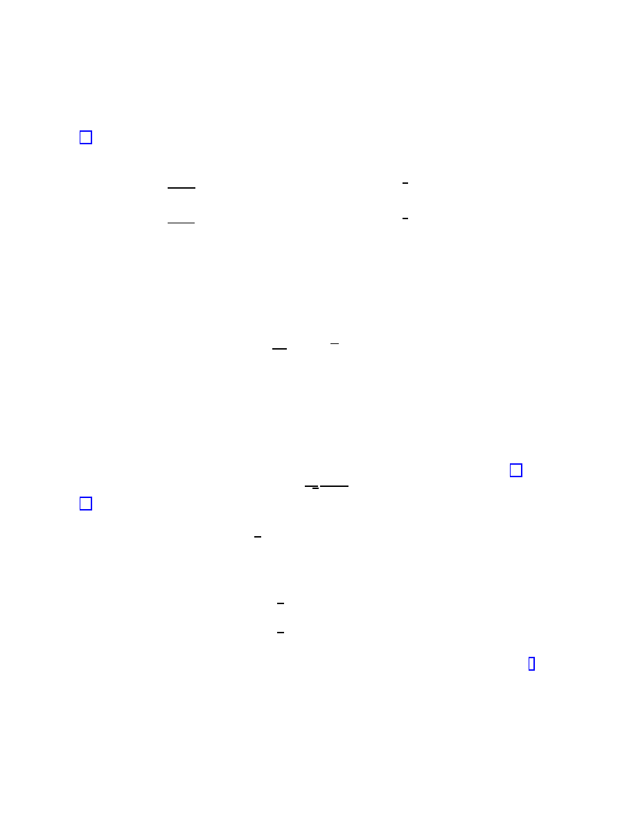
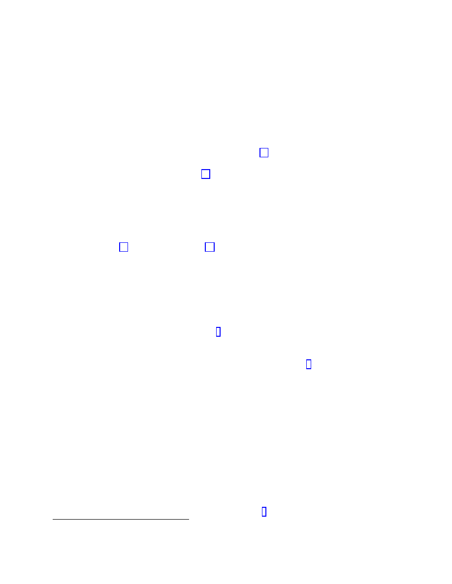
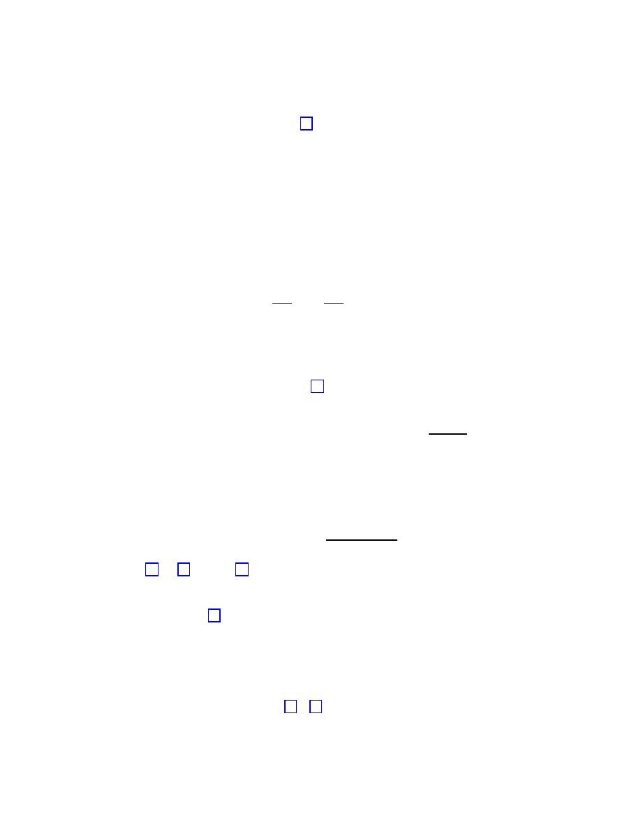
j
k
i
α
α
i
jk
g
j
0
g
k
0
g
i
1
= −
1
y
i
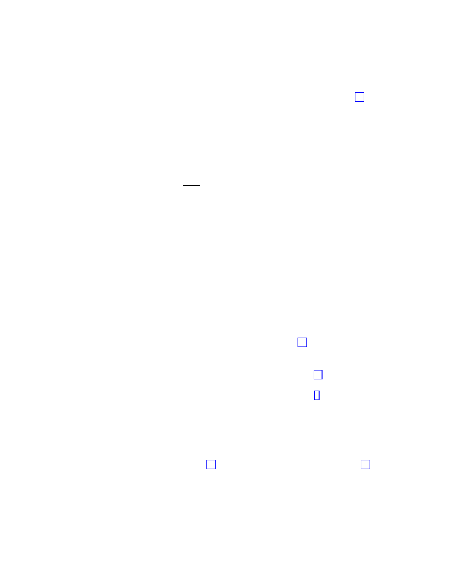
Conformal Invariance Condition:
Three−Tachyon Scattering Amplitude
=
j
k
i
j
k
i
m
m
+
γ
α
α
j
k
m
i
g
2
i
=
α
i
α
jn
n
km
y
n
γ
i
jkm
g
g
g
0
0
0
j
k
m
Four−Tachyon Scattering Amplitude
Conformal Invariance Condition:
Figure 4: Schematic representation of the equivalence of conformal invariance conditions
(vanishing of world-sheet renormalization group β-functions) and on-shell string scattering
amplitudes in the case of an open string in a tachyonic background.
The corresponding conformal invariance condition can be found by iterating the one at
previous order as follows: the first order result yields y
i
g
i
0
= 0; to second order we write
for the coupling g
i
= g
i
0
+ g
i
1
, which then, on account of the vanishing of the β-function
β
i
= y
i
g
i
+ α
i
jk
g
j
g
k
+ . . . = 0, yields:
g
i
1
=
−
1
y
i
α
i
jk
g
j
0
g
k
0
(81)
The situation is depicted in figure 4. It represents a three-tachyon scattering amplitude,
with two external legs set on-shell, and with one propagator pole at y
i
= 0. If one sets this
third leg on shell two, then the residue of the pole is the three-on-shell tachyon scattering
amplitude.
Higher orders in ˜
T
R
(k): at the next level one obtains a highly non-trivial demonstration
of the above-mentioned equivalence between conformal invariance conditions and on-shell
S-matrix elements. We shall not give details here, as these can be found by the interested
reader in the literature [5]. Below we shall only outline the results. Schematically the
situation is depicted in fig. 4.
24

Following a similar treatment as before, but encountering signficantly more complex
mathematical manipulations, one obtains as a solution of the conformal invariance condi-
tions to this order:
g
i
2
=
1
y
i
α
i
jm
α
m
k`
y
m
− γ
i
jk`
!
g
j
0
g
k
0
g
`
0
,
γ
i
jk`
g
j
0
g
k
0
g
`
0
=
−D
i
jk`
+
2α
i
jm
α
m
k`
y
j
+ y
m
− y
i
!
g
j
0
g
k
0
g
`
0
(82)
where, in the tachyonic background open string case, the contact terms of the graph are:
D
k
k
1
k
2
k
3
=
δ
(26)
(k
1
+k
2
+k
3
−k)
1+B+C
3
F
2
(1,
− 1 − B − C, − C, − 1 − A − B − C, − B − C; 1),
with
3
F
2
denoting a hypergeometric function, and A = 2k
1
· k
2
, B = 2k
1
· k
3
, C = 2k
1
· k
3
,
and 2 + A + B + C = y
j
+ y
k
+ y
`
− y
i
, with y
i
the anomalous dimensions defined above.
This completes the demonstration on the equivalence of the conformal invariance con-
ditions of a stringy σ-model with string scattering amplitudes. As we have discussed above
such amplitudes can be reproduced by a target space diffeomorphism invariant effective
action. The form of this action can be most easily obtained if one folows the second method
of perturbative expansion for computing the β-functions, the so-called Regge-slope α
0
ex-
pansion, which from now on we shall restrict ourselves upon. For simplicity, in these
lectures we shall restrict ourselves to
O(α
0
) in this expansion. This will be sufficient for
our cosmological considerations. Some comments on higher orders will be made where
appropriate.
2.7.2
Regge-slope (α
0
) expansion:
O(α
0
)-Weyl anomaly Coefficients
The second method of perturbative σ-model expansion, which we shall make use of in the
context of the present lectures, consists of expanding the partition function, correlation
functions and β-functions in powers of α
0
, or rather in the dimensionless quantity α
0
k
2
,
where k
M
is a target momentum contravariant vector (for open strings the expansion is
actually made in powers of
√
α
0
k). The Regge slope α
0
-expansion is independent of the g
i
-
expansion, studied above, but formally it is equivalent to that, in the sense that the exact
expressions (resummed to all orders) of the pertinent σ-model partition function in both
expansion methods contain the same physical information. In practice, the α
0
expansion
is appropriate if one is interested, as we are in the cosmological context of these lectures,
in long-wavelength (compared to Planck scales) effective actions. In such a case the first
few orders in the α
0
expansion (actually up to and including
O(α
0
) ) will suffice to provide
an adequate description of the observed Universe, as we shall discuss in Lecture 2.
In these lectures we shall not discuss in detail the very intersting techniques underlying
the α
0
-expansion of σ-model renormalization-group analysis. The interested reader may
find details on this in the vast literature [1]. For our purposes here, we shall merely quote
the results for the
O(α
0
) Weyl anomaly coefficients for Bosonic (or better the bosonic part
of) σ-model backgrounds of graviton, antisymmetric tensor and dilaton fields.
For such backgrounds in the Bosonic string case (for definiteness) we have:
25
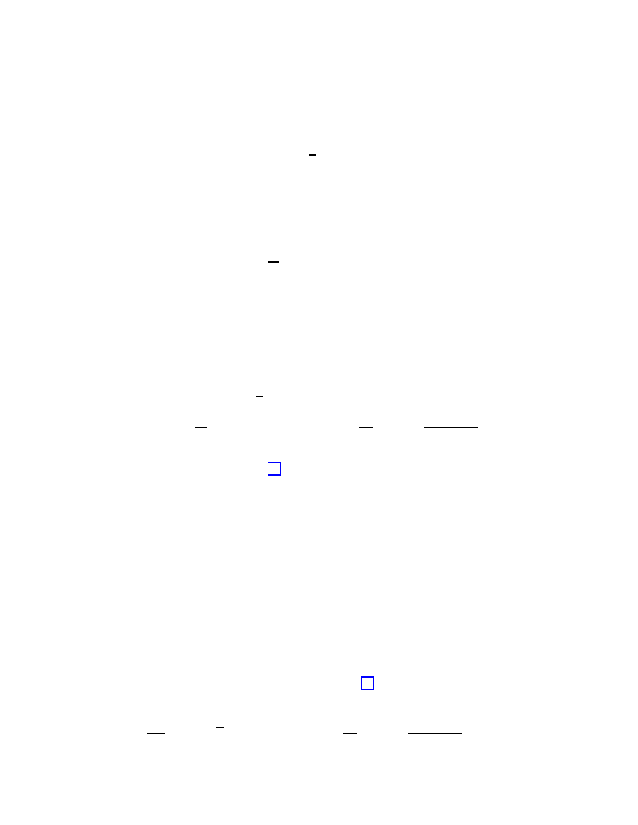
• Graviton: For the Weyl anomaly coeffcient of the graviton background one has:
b
β
g
M N
= α
0
R
M N
−
1
4
H
P Q
M
H
N P Q
+ 2
∇
(M
∂
N )
Φ
(83)
where the last part (depending on Φ) may be attributed to the differomorphism δg
i
part of the Weyl anomaly coefficient.
• Antisymmetric Tensor: For the antisymmetric tensor backgrounds one finds:
b
β
B
M N
=
α
0
2
−∇
P
H
P
M N
+ 2(∂
P
Φ)H
P
M N
(84)
where again the dilaton (Φ) dependent part is attributed to target-space diffeomor-
phism parts.
• Dilaton Fields: For dilaton fields it is convenient, for reasons that will become clear
below, to define a Weyl anomaly coefficient with the (target-space) gravitational trace
of graviton Weyl anomaly coefficient subtracted:
˜
b
β
Φ
=
b
β
Φ
−
1
4
g
M N
β
g
M N
=
α
0
4
−4(∂
M
Φ)
2
+ 4
∇
2
Φ + R
−
1
12
H
2
M N P
−
2(D
− 26)
3α
0
!
(85)
Notice in the last expression (85) that the appearance of the scalar curvature is an
exclusive consequence of the presence of the trace of the graviton Weyl anomaly
coefficient in
˜
b
β
Φ
. The dilaton Weyl anomaly coefficient, to
O(α
0
) does not depend on
the target-space curvature, only on derivatives of the dilaton field. Moreover, we also
notice that to zeroth order in α
0
, the dilaton Weyl anomaly coefficient does depend
on the conformal anomaly D
− 26, which is absent for critical dimension strings.
This term, if present, would act as an exponential dilaton potential (or equivalently
vacuum energy ). In the critical dimension D
c
= 26 (for bosonic strings) is absent.
We shall come back to this important issue in our third lecture, when we discuss the
issue of cosmological constant in the context of string theory. For superstrings the
D
− 26 term is replaced by D − 10, and the vacuum energy term is absent for the
case of critical superstring space-time dimension D
c
= 10.
We now notice that, as can be shown straightforwardly, the vanising of the above
expressions (i.e. the conformal invariance conditions (64) for this set of background fields)
corresponds to equations of motion of a low-energy
O(α
0
) target-space effective action:
I
eff
=
−
1
2κ
2
Z
d
D
X
√
ge
−2Φ
R + 4(∂
M
Φ)
2
−
1
12
H
2
M N P
−
2(D
− 26)
3α
0
+ . . .
!
(86)
26
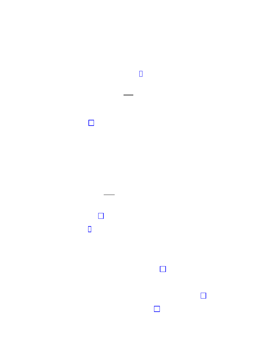
where κ
2
is the Gravitational constant in D target space time dimensions (related appro-
priately to the Planck (or string) mass scale M
s
).
In fact, as mentioned earlier in the context of g
i
weak field expansion, it can also
be shown explicitly within the α
0
expansion [6], that the above-mentioned Weyl anomaly
coefficients
b
β
i
are gradient flows in g
i
space of I
eff
:
δI
eff
δg
i
=
G
ij
b
β
j
(87)
where, up to appropriate field redefinitions, which are irrelevant from the point of view
of scattering amplitudes, as they leave them invariant, the function
G
ij
coincides with the
Zamolodchikov metric (61).
2.7.3
World-Sheet Renormalizability Constraints on the
b
β-functions
The world-sheet renormalizability of the σ-model action, deformed by background fields
g
i
, i.e. the fact that this two-dimensional theory has ultraviolet divergencies which can
be absorbed in appropriate redefinition of its coupling/fields g
i
, without the necessity for
introducing new types of interactions that do not exist in the bare theory, is expressed
simply in terms of the renormnalization-group scale invariance of the components of the
world-sheet stress tensor of the theory:
d
dlnµ
T
αβ
= 0 ,
α, β = σ, τ
(88)
where lnµ is the renormalization-group scale.
Equations of the type (88) implies severe constraints among the
b
β-functions which,
after some elegant σ-model renormalization-group analysis, are expressed by means of the
Curci-Paffuti equation [7]. To order α
0
this equation reads:
∇
N
b
β
Φ
= 2g
M P
e
−2Φ
∇
N
e
−2Φ
b
β
g
M P
+
O(
b
β
B
)
(89)
An immediate consequence of this equation is that not all of the
b
β
i
= 0 equations are
independent. In particular, at a fixed point of the renormalization-group on the world-
sheet, for which
b
β
g
M N
=
b
β
B
M N
= 0, one obtains from (89) that the dilaton Weyl anomaly
coefficient is constant, not necessarily zero. In the particular case of strings in Bosonic
massless backgrounds, for instance, this constant is simply the conformal anomaly D
− 26
(Bosonic Strings) or D
− 10 (Superstrings).
When discussing equations of motion the Curci-Paffuti constraint (89) should always
be taken into account. Although the constraint may seem trivial in case one is interested
in solutions of the confornal invariance conditions (64),
b
β
i
= 0, this is not the case when
one encounters non-trivial
b
β
i
6= 0 away from the fixed points of the renormalization group
on the world sheet. Such a situation (non-critical Strings) may be of interest in non-
equilibrium cosmological situations, and we shall discuss it briefly in Lecture 3.
27
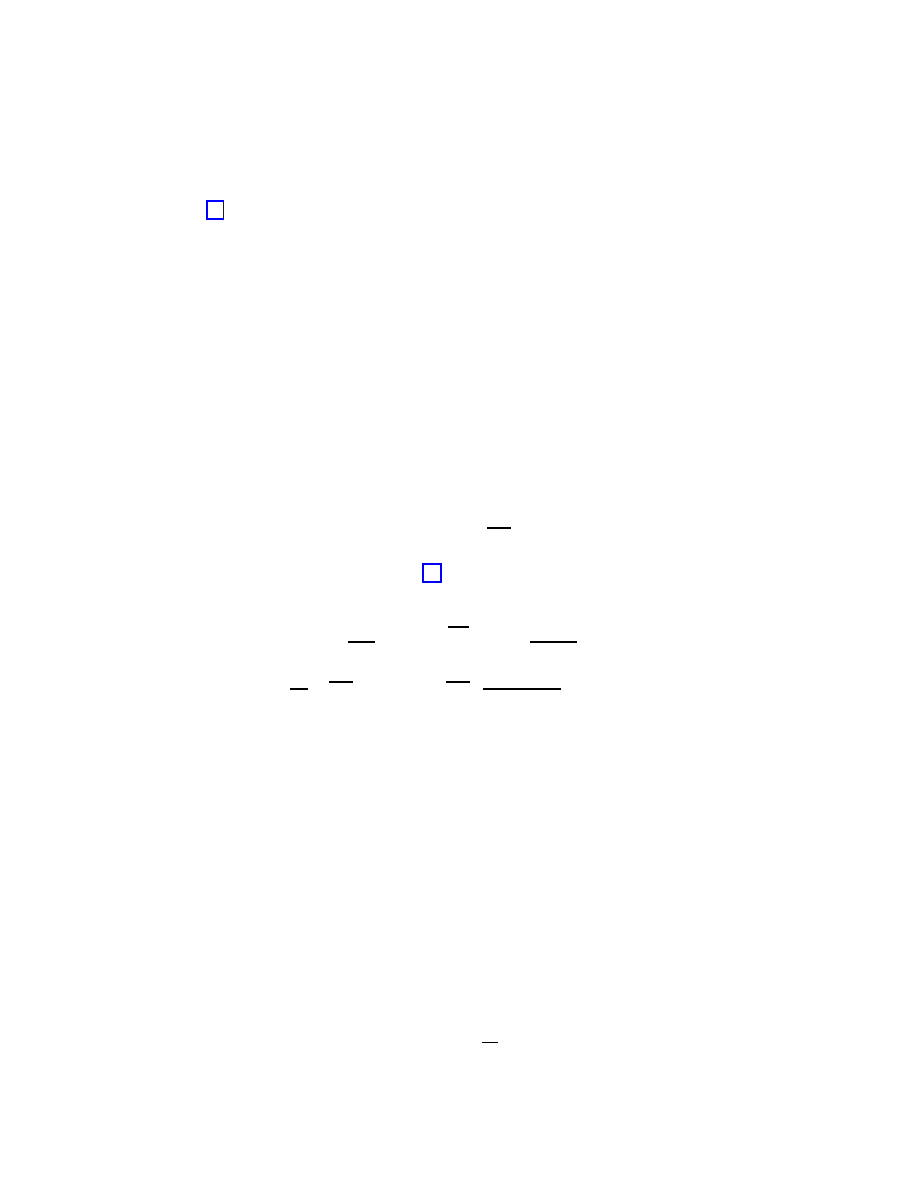
2.7.4
A note about “Frames”
The action (86) is derived in the so-called σ-model frame, because it is derived directly
from expressions obtained in σ-model renormalization-group ananlysis. Such a terminol-
ogy should not be confused with the general coordinate frames in general relativity. The
terminology “frame” here is used to mean a given background metric configuration. In
string theory, the perturbative string S-matrix elements (scattering amplitudes) are in-
variant under local redefnition of the background fields g
i
(“equivalence theorem”), which
simply corresponds to a particular renormalization-group scheme choice.
The σ-model frame metric corresponds to one such configuration. One may redefine
the metric field so as to pass to an effective action, where the curvature scalar term in
the action will have the standard (from the point of view of General relativity) coefficient
1/κ
2
, without the dilaton conformal factor e
−2Φ
in front. In other words, it will have
the canonically normalized Einstein action form. Such a “frame”, termed Einstein (or
“physical”) frame, is obtained upon redefining the σ-model background metric as follows
(the superscript E denotes quantities in the Einstein frame):
g
M N
→ g
E
M N
= e
−
4
D
−2
Φ
g
M N
(90)
In this frame, then, the effective action (86) acquires, as mentioned already, its canonical
Einstein form, as far as the gravitational parts are concerned:
I
E
eff
=
−
1
2κ
2
Z
d
D
X
q
g
E
R
E
−
4
D
− 2
(∂
M
Φ)
2
−
1
12
e
−
8
D
−2
Φ
H
2
M N P
− e
4
D
−2
Φ
2(D
− 26)
3α
0
+ . . .
!
(91)
where the . . . denote higher-order terms, as well as other fields, such as gauge-boson terms
(in the case of heterotic string) etc. Notice the change of relative sign between the curvature
and dilaton kinetic terms in the Einstein frame.
From the point of view of discussing physical low-energy applications of string theory,
such as cosmological models based on strings, the Einstein frame is the “physical” one,
where the astrophysical observations are made. This will always be understood when we
discuss string cosmology in Lectures 2 and 3.
2.7.5
Higher orders in α
0
Corrections to General Relativity occur at the next order in α
0
, at which one can show, for
instance, that the graviton β-function has the form (ignoring the contributions from other
backgrounds for simplicity):
β
g
M N
(X
P
) =
−α
0
R
M N
+
α
0
2
R
M KLP
R
N
KLP
!
(92)
28

The higher-curvature terms will result in corrections to the Einstein term in the target-
space effective action. Such action terms have some ambiguities concerning their coeffi-
cients, since the scattering S-matrix elements one derives from an effective action corre-
spond to more than one set of these coefficients (the equivalence theorem, mentioned earlier
in the Lecture). The amplitudes are invariant under ocal redefinitions of the graviton field
(in this case): g
M N
→ g
M N
+ cα
0
R
M N
, where c a constant coefficient. Such redefinitions
affect the higher order in α
0
terms of the target-space effective action, in such a way that
one can always cast it in the Gauss-Bonnet (gravitational ghost-free) combination:
S =
Z
d
D
x
√
g
R + αα
0
R
2
M N RP
− 4R
2
M N
+ R
2
+ . . .
(93)
where the coefficient α is determined by comparison with string tree amplitudes. It is found
to be: α = 1/4 (Bosonic String), α = 0 (Superstring type II), and α = 1/8 (Heterotic
string).
The fact that stringy higher-order corrections to the low-energy effective actions of
string theories are free from gravitational ghosts, in the sense that the effective action can
always be cast, under local field redefinitions, in the ghost-free Gauss-Bonnet combination,
is consistent with the unitarity of the underlying string theory.
The higher-order corrections to Einstein’s general relativity are in principle an infinite
series of terms, which become stronger at high energies (short distances). From a cosmo-
logical viewpoint, the higher-curvature terms may thus have effects at very early stages of
our Universe, but such effects are negligible at redshifts z
∼ 1 and lower, where we shall
concetrate most of our discussion in these lectures. One should notice that the presence of
higher-curvature correction terms of Einstein’s general relativity leads some times to highly
non-trivial effects. For instance, one may have black hole solutions with (secondary) dila-
ton hair [8] in such models, which do not exist in standard Einstein’s relativity. Such
objects may play a rˆole in the Early Universe.
3
Lecture 2: String Cosmology
3.1
An Expanding Universe in String Theory and the rˆ
ole of the
Dilaton Background
As has already been discussed in the cosmology lectures in this School, the Observed
Universe is, to a good approximation, homogeneous and isotropic. From the point of view
of string theory, therefore, one is interested in describing the propagation of strings in such
homogeneous backgrounds, i.e. space-time geometries whose metric tensors depend only
on time, and thus have no spatial dependence.
As we have discussed in the previous lecture, conformal invariance conditions (64) of the
associated σ-model will imply target-space equations of motion for the background fields,
which will determine the dynamics. This is, in general terms, what String Cosmology is
about. The pertinent dynamics will be described by means of string effective actions for
29
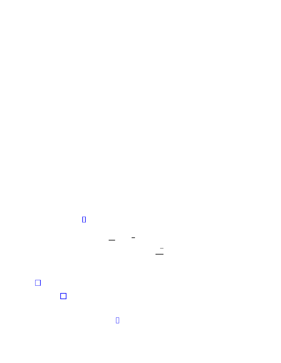
the various (time dependent only) modes. Of course, this is a first order approximation.
Spatial Inhomogeneities can be incorporated by allowing spatial dependence of the various
σ-model couplings/background fields.
It is the purpose of this part of the lectures to discuss how one can incorporate expanding
Universe scenaria in the above string context. We shall start with the simplest scenario,
that of a linearly expanding non-accelerating Universe. Subsequently we shall discuss more
complicated models, including inflationary scenaria in string theory, and mechanisms for
graceful exit from it. Due to lack of time, the discussion will be relatively brief. For more
details, the interested reader will be referred to the literature, which is vast, and still
growing. In the last two lectures I will try to give whatever details, and technical aspects,
I believe are essential for introducing the layman into the subject of string cosmology and
make him/her understand the various subtleties involved. It should be stressed that string
cosmology is not a physically well established subject, and part of the third lecture will be
devoted to discussing open issues, motivated by recent astrophysical observations on the
possibility of a currently accelerating phase of the Unvierse, and the way such issues can
be tackled in the framework of string theory.
In all stringy cosmological scenaria of expanding Universes that we shall examine here
the dilaton plays a crucial rˆole, as being directly responsible for providing consistent time-
dependent backgrounds in string theory. This is an important feature which differentiates
string cosmology from conventional one (this feature is, of course, in addition to the fact
that the target-space dimensionality of string theory is higher than four).
We commence our discussion by considering the σ-model action of a string propagating
in time-dependent backgrounds of graviton g
M N
, antisymmetric tensor B
M N
and dilatons
Φ. Although given in Lecture 1, for completeness we give again the action explicitly (in
this subsection we work in units of α
0
= 2 (closed strings) for convenience, and we follow
the normalization of [9] for the dilaton field, which implies that the dilaton field here equals
twice the dilaton field in the previous section):
S
σ
=
Z
Σ
1
4π
d
2
σ
√
γγ
αβ
g
M N
(X
0
)∂
α
X
M
∂
β
X
N
+
B
M N
(X
0
)
αβ
∂
α
X
M
∂
β
X
N
+
√
γ
2
Φ(X
0
)R
(2)
!
(94)
where M, N = 0, . . . , D
− 1, and X
0
denotes the target time. The reader is required to
remember that the dilaton coupling is of one order in α
0
higher than the rest of the terms in
(94). As already mentioned, the time dependence of the backgrounds is appropriate for a
discussion of isotropic and homogneoeus cosmological solutions of the conformal invariance
conditions (64), which we now turn to.
3.1.1
Linear Dilaton Background Conformal Field Theory
Consider the σ-model background [9]:
g
M N
= η
mn
, B
M N
= 0, Φ =
−2QX
0
,
Q = const
(95)
30
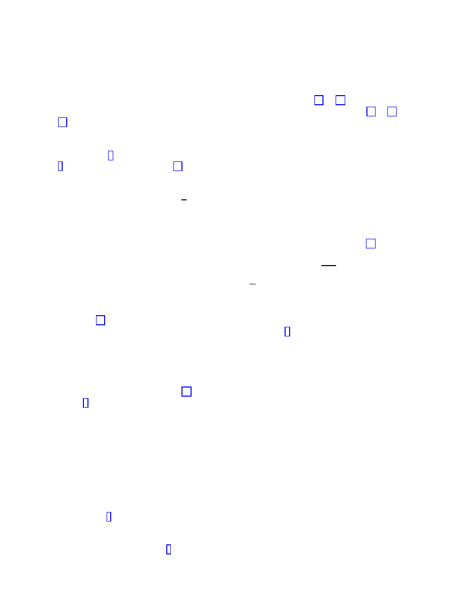
in which the dilaton is growing linearly with the target time. We observe that this is
an exact solution of the σ-model conformal invariance conditions (64), (89), for the Weyl
anomaly coefficients, which, for the problem at hand, and to
O(α
0
) are given by (83), (84),
(85). Hence it is an acceptable background in string theory.
Let us describe the basic features of this conformal theory. We wish to determine first
the central charge (conformal anomaly). To this end we need to compute the world-sheet
stress tensor [1]. As we have discussed in Lecture 1, the latter is defined by the response
(9) of the world-sheet action (94) to a variation of the world-sheet metric. The presence
of the dilaton term results in the following form:
T
zz
=
−
1
2
∂
z
X
M
∂
z
X
N
g
M N
(X
0
) + Q∂
2
z
X
0
(96)
where z is the complexified world-sheet coordinate (we work in a Euclidean world-sheet,
appropriate for the convergence of the σ-model path integral formalism we adopt here).
[ NB4: For completeness we sketch below the derivation of the Q∂
2
z
X
0
term in (96). This
comes from varying the world-sheet curvature/dilaton term with respect to the world-sheet
metric, and setting at the end γ
αβ
= δ
αβ
(for Euclidean world sheets):
δ
δγ
αβ
R
Σ
R
(2)
QX
0
(σ, τ ).
Noticing that only contributions from the second derivatives of the world-sheet metric in
R
(2)
survive this procedure, we obtain:
R
Σ
d
2
σ
0
√
γ∂
2
z
δ
(2)
(σ
− σ
0
)Qt(σ
0
) =
−
R
Σ
δ
(2)
(σ
−
σ
0
)Q∂
z
0
t =
−Q∂
2
z
t, where partial integration has been made in order to arrive at the last
equality ].
From (96) it is straightforward to compute the conformal anomaly c. From basic
conformal field theory we recall that the latter is given by [1]):
lim
z
→0
2z
4
hT
zz
(σ)T
zz
(0)
i = c
(97)
Regulating the short-distance behaviour of the theory by replacing z
→ 0 by z → a,
where a is a short-distance cutoff scale, and using the free-field contractions for two-point
correlators on the world-sheet (71) (with ξ(x
1
)
←→ X
M
(σ) ) it is straightforward to
derive [9]:
c = D
− 12Q
2
(98)
where D is the dimensionality of the target-space time.
This is an important result. In the conformal field theory of a non-trivial linear dilaton
background, and flat σ-model target spacetime, the conformal anomaly is no longer given
by the target-space dimensionality D alone, which was the case of Minkowski space times,
as we have seen in Lecture 1.
The cancellation of the Weyl anomaly implies c = 26 (for bosonic strings, which we
restrict ourselves from now on for definiteness, unless otherwise stated). This, therefore,
means that the critical dimensionality of the string is D > 26. This string theory is termed
supercritical [9].
The non-trivial issue is to demonstrate the mathematical consistency of such string
theories, by demonstrating unitarity of the physical spectrum, and modular invariance,
associated with string loops [1]. We note that both of these properties have been shown to
31
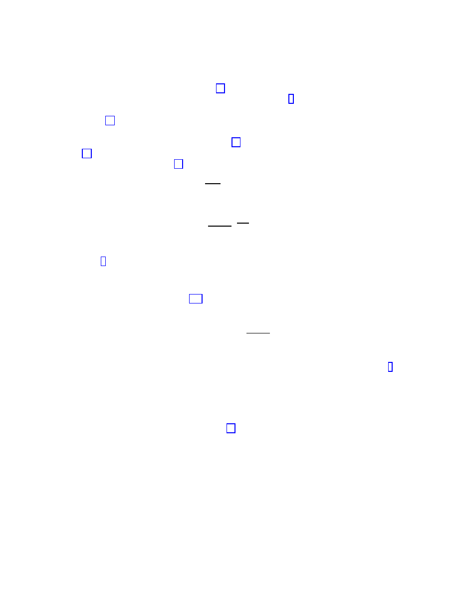
be valid for the linear dilaton background (95). We shall not demonstrate them here due to
lack of time. We refer the interested reader to the literature [9] for a detailed verification.
We next proceed to discuss the target-space time interpretation of the linear dilaton
background (95). As we have mentioned previously, the ‘physical’ metric, appropriate
for cosmological considerations in theories with non-trivial dilaton fields, is provided by
the Einstein frame target-space metric tensor (90), corespondiong to a low-energy effective
action (91) with canonically-normalized Einstein curvature term, without dilaton conformal
factors. For the background (95), therefore, the Einstein-metric invariant line element
reads:
ds
2
E
= e
4QX0
D
−2
η
M N
dX
M
dX
N
(99)
Upon redefining the time X
0
→ t:
t =
D
− 2
2Q
e
2Q
D
−2
X
0
(100)
we observe that the Einstein (“physical”) metric may be cast into a Robertson-Walker
(RW) form [9]:
ds
2
E
=
−(dt)
2
+ t
2
dX
i
dX
j
δ
ij
(101)
with a linearly expanding in time t, non accelerating scale factor a(t) = t,
¨a(t)
≡
d
2
a(t)/dt
2
= 0. The RW Universe (101) has zero spatial curvature, i.e. is flat.
In these coordinates the dilaton field has a logarithmic dependence on time:
Φ(t) = (2
− D)ln
2Qt
D
− 2
(102)
One may accommodate more general RW backgrounds with non-trivial spatial curva-
ture in the above framework, by including non-trivial antisymmetric tensor backgrounds [9].
This is what we shall discuss below.
3.1.2
The antisymmetric tensor field and More General Cosmological Back-
grounds
First of all we concentrate our attention to (98). We assume that in our model there are
d = 4 “large” (non-compact) target-space time dimensions, one of which is the Minkowski
time. The rest of the target dimensions (6 in the case of superstring, or 22 in the case of
Bosonic strings) are replaced by an appropriate “internal” conformal field theory with a
central charge c
I
:
c = d + c
I
− 12Q
2
= 4 + c
I
− 12Q
2
(103)
Notice that the total central charge c is required to equal its critical value (26 for Bosonic
strings, 10 for superstrings) so as to ensure target-space diffeomorphism invariance (i.e. to
cancel the Fadeedv-Popov reparametrization ghost contributions to the conformal anomaly),
32
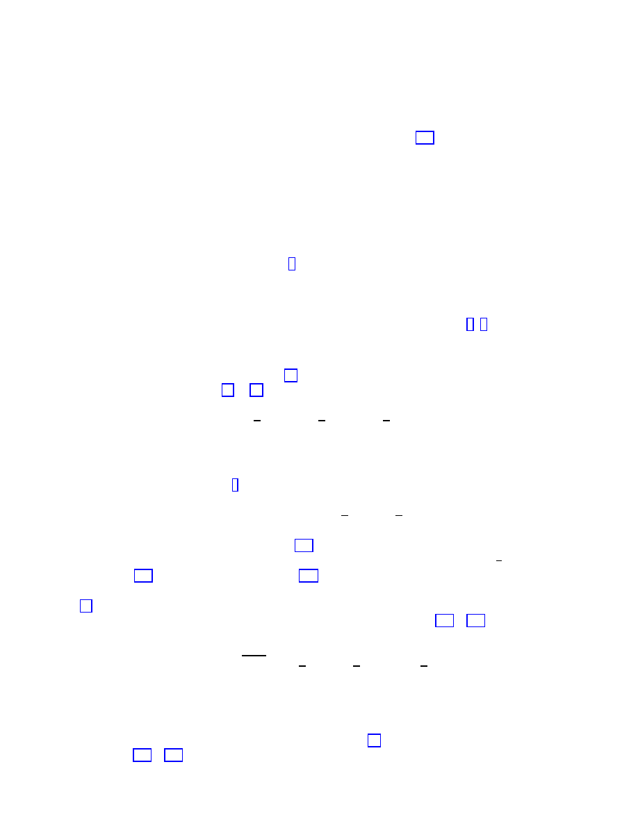
and also conformal invariance of the complete theory. These two requirements are essen-
tial for giving string theory a space-time interpretation. Then (103) leads to (for Bosonic
strings for brevity):
c
I
= 22 + 12Q
2
≡ 22 + δc
(104)
where δc is known as the central charge deficit. For a critical dimension string theory,
δc = 0.
From now on we shall ignore the details of the compact internal theory, and simply
assume it is there to ensure the above properties, and hence consistency, of the string the-
ory at hand. One can show that non-trivial internal conformal field theories can indeed be
constructed with the desired properties [9]. We therefore consider d = 4-dimensional back-
grounds g
µν
(x), B
µν
(x), Φ(x), where µ, ν = 0, . . . 3, and x
µ
are four-dimensional spacetime
coordinates.
In four space time dimensions the antisymmetric tensor field strength may be written
in terms of a pseudoscalar field b(x) to be identified with the axion field [1, 9]:
H
λ
µν
= e
2Φ
λ
µνρ
∂
ρ
b
(105)
The conformal invariance conditions (64), then, corresponding to the four-dimensional
Weyl anomaly coefficients (83), (84) read:
graviton :
R
µν
=
1
2
∂
µ
Φ∂
ν
Φ +
1
2
g
µν
∇
2
Φ +
1
2
e
2Φ
[∂
µ
b∂
ν
b
− g
µν
(∂b)
2
],
antisym. tensor :
∇
2
b + 2∂
λ
b∂
λ
Φ = 0
(106)
The fact that the total central charge is 26 (for Bosonic strings, or 10 for superstrings)
implies the dilaton equation [9]:
δc = 12Q
2
=
−3e
−Φ
−R + ∇
2
Φ +
1
2
(∂Φ)
2
−
1
2
e
2Φ
(∂b)
2
(107)
(in units α
0
= 1), where δc is defined in (104). We stress again that in the case of critical
strings δc would vanish. Here, as a result of the Bianchi identity
∇
µ
R
µν
=
1
2
∇
ν
R, the
equations (106) imply the consistency of (107), i.e. that the right-hand-side is a constant,
consistent with δc=const. This consistency is nothing other than the Curci-Paffuti equation
(89), stemming from renormalizability of the world-sheet σ-model theory.
The four-dimensional effective low-energy action obtained from (106),(107), in the Ein-
stein frame, is:
I
eff
=
Z
d
4
x
q
−g
E
R
−
1
2
(∂Φ)
2
−
1
2
e
2Φ
(∂b)
2
−
1
3
e
Φ
δc
(108)
Note that, as a result of the non-trivial central-charge deficit δc
6= 0, there is a non-
vanishing potential for the “internal” fields, which implies a non-trivial vacuum energy
term for a four-dimensional observer.
We note now that the linear dilaton background (95) is indeed a special case of the
equations (106),(107), leading in the Einstein frame, to spatially flat RW linearly expanding
33
Universes,as we have seen above, . For non trivial axion fields b one has more general RW
backgrounds, with spatial curvature. Indeed, it can be shown that the equations (106),(107)
admit as solution [9]
ds
2
E
=
−dt
2
+ a(t)
2
˜
g
ij
dx
i
dx
j
, i, j = 1, 2, 3
(109)
where ˜
g
ij
is a three-dimensional maximally symmetric metric:
˜
g
ij
dx
i
dx
j
=
dr
2
1
− kr
2
+ r
2
(dθ
2
+ sin
2
θdφ
2
)
(110)
where t is the phhysical time (100), and the RW parameter k, related to spatial curvature,
is to de determined below.
The Hubble parameter is given by: H(t)
≡
˙a(t)
a(t)
, with the dot denoting derivative w.r.t.
t. With the ansatz (109), (110) the antisymmetric tensor/axion equation in (106) is solved
by [9]:
˙b = b
0
e
−2Φ
a(t)
3
,
b
0
= const.
(111)
and the dilaton equation (107) implies for the central-charge deficit:
δc = 6e
−Φ
˙
H + 3H
2
+
2k
a(t)
2
!
(112)
The graviton equations have in principle two independent components:
µ = ν = t :
−6( ˙
H + H
2
) = ¨
Φ + 3H ˙
Φ + ( ˙
Φ)
2
,
µ, ν = i, j :
−2( ˙
H + 3H
2
+
2k
a(t)
2
) = ¨
Φ + 3H ˙
Φ
−
b
2
0
a(t)
6
!
e
−2Φ
(113)
However, since the dilaton equation (107) is an identity (up to an irrelevant constant),
one observes actually that there is only one independent equation for the graviton. In-
deed, solving (112) for the dilaton and substituting into (113), and subtracting these two
equations we obtain:
¨
H + 6 ˙
H H
− (4k/a(t)
2
)H
˙
H + 3H
2
+ 2k/a(t)
2
!
2
=
−4 ˙
H +
4k
a(t)
2
−
(δc)
2
b
2
0
36a(t)
6
·
1
˙
H + 3H
2
+ (2k/a(t)
2
)
2
(114)
This equation can in principle be solved, yielding the Hubble parameter for the string
Universe under consideration.
Asymptotic Solutions of (114): There are two kinds of asymptotic solutions, of (114),
which can be obtained analytically:
34
• (I) H → 0, as t → +∞, Φ = φ
0
=constant, ˙b = b
0
e
−2φ
0
and the space curvature
obeys
k =
1
4
b
2
0
e
−2φ
0
≥ 0
(115)
and thus is non negative. This Universe is therefore closed. The central charge deficit,
in this case is determined via the dilaton equation (107) to be : δc = 12e
−φ
0
k. This
asymptotic Universe is therefore a static Einstein Universe with non-negative spatial
curvature.
• (II) A linearly expanding Universe a(t) = t with metric:
ds
2
E
=
−(dt)
2
+ t
2
"
dr
2
1
− kr
2
+ r
2
(dθ
2
+ sin
2
θdφ
2
)
#
(116)
with Hubble parameter relaxing to zero as t
→ ∞ as: H(t) ∼ 1/t, and hence one
has:
Φ =
−2lnt + φ
0
,
b = 2e
−φ
0
√
kt
(117)
with k again non-negative. The four-dimensional curvature is R = 6(1 + k)/t
2
, and
the central charge deficit is δc = 12e
−φ
0
(1 + k).
Conformal Field Theories corresponding to the asymptotic solutions (I) and
(II)
The asymptotic solutions, found above to leading order in α
0
, can become exact solutions
if one manages to construct explicitly the corresponding conformal fied theories (CFT) on
the world shweet.
This has been done in some detail in [9]. Below we only describe the main results. For
the static Einstein Universe the corresponding CFT is a two-dimensional Wess-Zumino
model on a O(3) group manifold, with a time coordinate which is a free world-sheet field.
The corresponding central charge is:
c = 1 +
3˜
κ
˜
κ + 1
= 4
−
3
˜
κ + 1
(118)
where ˜
κ is the Wess-Zumino level parameter of the O(3) Kac-Moody algebra. The central
charge deficit (104) is in this case:
δc =
3
˜
κ + 1
= 12e
−φ
0
k + . . .
(119)
where . . . denote higher orders. The important point to notice is that the level parameter
˜
κ is an integer for topological reasons (equivalently, this result follows from unitarity of the
spectrum and modular invariance of the underlying string theory [9]). Thus, (119) implies
that the central charge deficit is quantized.
The conformal field theory corresponding to the second asymptotic solution (II) of
(114), that of a linearly expanding Unviverse, can be found most conveniently if we go
35
back to the σ-model frame: g
µν
= e
Φ
g
E
µν
and the σ-model coordinate time X
0
(100), in
wich the dilaton is linear:
Φ =
−2e
−φ
0
/2
X
0
+ φ
0
≡ −2QX
0
+ φ
0
(120)
Thus we observe that Q
≡ e
−φ
0
/2
plays the rˆole of a “charge at infinity” in similar spirit
to the Coulomb-gas conformal models [1], an analogy prompted by the form of the corre-
sponding stress tensor (96).
The corresponding world-sheet conformnal field theory is again a Wess-Zumino model
on a group manifold, in which g
ij
is the metric, and H
ij`
=
∇
[i
B
j`]
is the volume element.
The model has again a time coordinate but with a charge Q at infinity, as we have just
mentioned. The (two-dimensional) Lagrangian of the model is:
L
(2)
=
−(∂X
0
)
2
− QX
0
R
(2)
+
L
W ZW
(O(3))
(121)
where R
(2)
is the world-sheet curvature. The central charge is: c = 1
− 12Q
2
+ c
W ZW
with
the level parameter ˜
κ being related to the spatial curvature k as fllows:
k =
1
2Q
2
˜
κ
(122)
Since ˜
κ
∈ Z
+
U
{0} for topological (or, equivalently unitarity and modular invariance)
reasons, then k > 0 and the four-dimensional Universe is again closed. The 4-d curvature
is found again to be R = 6(1 + k)/t
2
.
3.1.3
The spectrum of the Linear-Dilaton Strings: Mass Shifts
Consider the conformal invariant solution (95). The corresponding Virasoro operators, i.e.
the moments of the world-sheet stress tensor, as we have discussed in the first Lecture,
are [9]:
L
n
=
1
2
X
j
η
µν
x
µ
n
−j
x
ν
j
+ iQ(n + 1)x
0
n
(123)
where x
µ
n
are moments of the world-sheet operators i∂
z
x
µ
, satisfying:
[x
µ
m
, x
ν
n
] = mη
µν
δ
m+n,0
,
x
µ
n
†
= x
µ
n
+ 2iQη
µ0
δ
n,0
(since L
†
n
= L
−n
)
(124)
This implies that the 0-th (time) component of Minkowski space-time momentum has a
fixed imaginary part [9]
p
0
= E + iQ
(125)
where the real part E corresponds to “energy”.
Consider for definiteness a bosonic scalar mode, e.g. a tachyon, which is the lowest
lying energy state of a Bosonic string (ground state):
|pi = e
−p
µ
x
µ
(0)
|0i
(126)
36
annihilated by all x
µ
n
(n > 0). The corresponding mass-shell condition is:
1
2
p
µ
p
µ
+ iQp
0
=
−
1
2
(E
2
+ Q
2
− ~p
2
) = 1
(127)
where ~
A denotes three-dimensional vectors. Thus, from (127) one observes that there is a
shifted mass for the tachyonic mode:
δm
2
T
= m
2
− Q
2
(128)
in such linear dilaton backgrounds.
From a target-spacetime view point, this can be easily understood considering the
Lagrangian for a scalar mode ϕ in the background (95) in the Einstein frame (90):
L
ϕ
= e
2Qx
0
−η
µν
∂
µ
ϕ∂
ν
ϕ
− m
2
ϕ
2
(129)
Indeed, rescaling the field ϕ
→ ˜
ϕ = e
Qx
0
ϕ, so as to have a canonical kinetic term, one
obtains a mode that obeys a free scalar-field wave equation, in flat space time, with shifted
mass (128).
This result can be extended to include all the other bosonic modes [9], including graviton
and dilaton. All such bosonic modes therefore will have a mass shift of tachyonic type in
supercritical strings:
δm
2
B
=
−Q
2
< 0
(130)
For target-space Supersymemtric strings, including the phenomenologically relevant
Heterotic string [1], in linear-dilaton backgrounds, one observes that there are no mass
shifts for the fermionic target space time modes [9].
This can be readily seen, for instance, by noting first that the anomaly condition for
superstrings becomes:
c
I
+ d
− 8Q
2
= 10
(131)
This is due to the additional stress tensor contributions on the world-sheet pertaining to
fermionic backgrounds T
F
=
−ψ
µ
∂
z
x
µ
+ 2Q∂
z
ψ
0
.
The lowest-lying fermionic excitations are massless, since superstrings do not have
tachyonic instabilities. Consider for simplicity the case c
I
= 0 and concentrate on the
lowest-energy Ramond state. Consider the moments of T
F
:
G
n
= i
X
n
ψ
µ
n
−m
x
µ,n
− 2Q(n + 1)ψ
0
n
(132)
When acting on the highest-weight state, one has:
G
0
=
−i (γ
0
E
− ~γ · ~p)
(133)
This is precisely the massless Dirac operator in flat space. Thus one observes that there is
no mass shift for the fermionic modes.
37
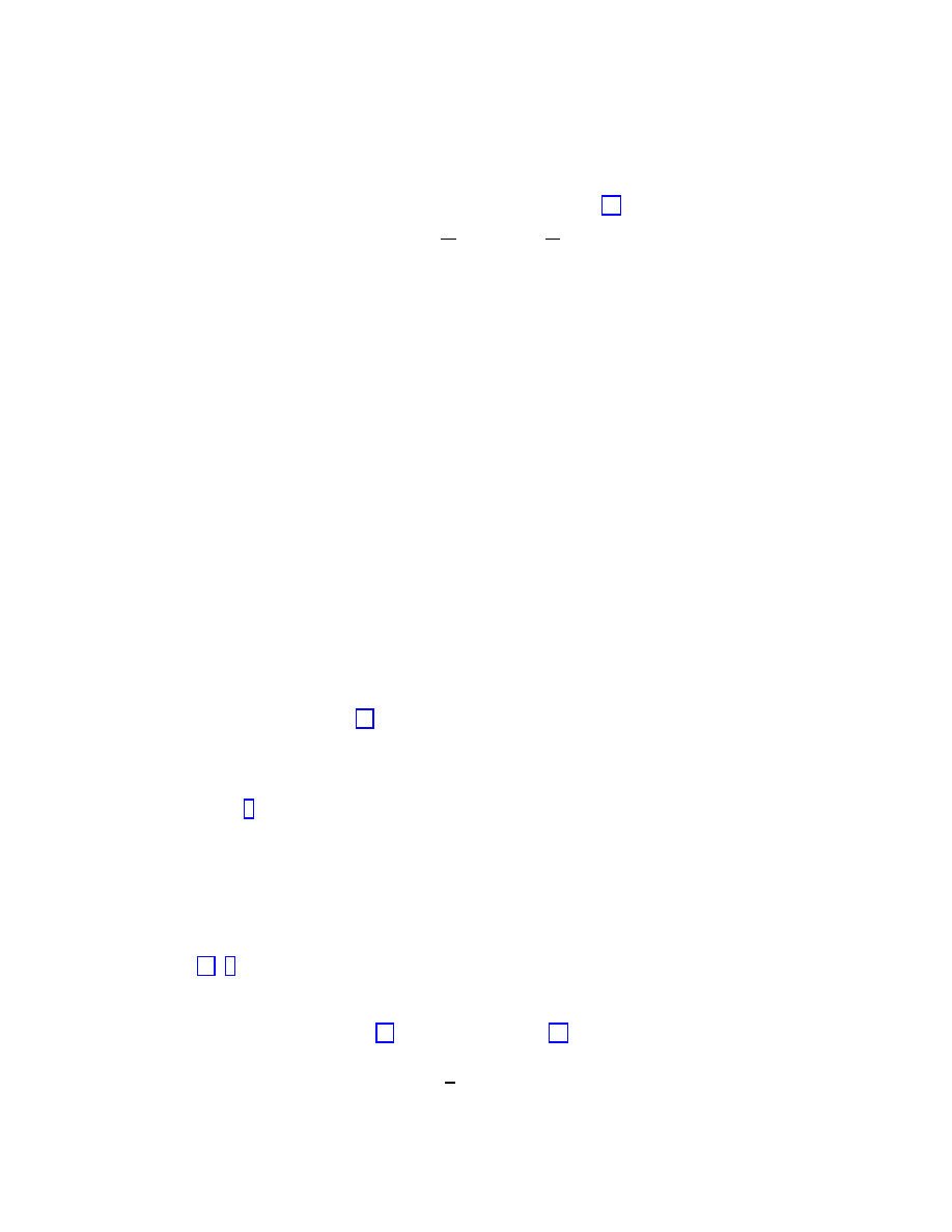
From a field-theoretic view point this can be seen from the quadratic part of the target-
space Lagrangian for fermionic modes Ψ, in the background (95):
L
fermion
= e
2Qx
0
Ψ∂
µ
γ
µ
Ψ + mΨΨ + . . .
(134)
It is easily seen that the rescaled fermion field ˜
Ψ = e
Qx
0
Ψ obeys the free Dirac equation
without a mass shift.
Thus, in a linear dilaton background, which leads to a linearly expanding Universe in
Einstein frame, there is no target-space fermionic-mode mass shift:
δm
2
F
= 0
(135)
So far, our considerations pertain to tree-level world-sheet σ-models, i.e. world-sheets
with the topology of a disc (open strings) or sphere (closed strings). String loop corrections
do affect the β-functions of the theory, and actually they do result in the appearance of
non-trivial dilaton potentials δV (Φ), whose effects we now come to discuss, from the point
of view of Cosmological backgrounds, which are of interest to us in the context of these
lectures.
3.2
String Loop Corrections and De Sitter (Inflationary) Space
Times
The string loop corrections, i.e. effects coming from higher world-sheet topologies, are non
trivial and they do modify the tree-level β-functions of the theory through the so-called
Fischler-Susskind mechanism [10]. To understand qualitatively the rˆole of such effects let
us consider the indicative example of a σ-model partition function on a world-sheet torus.
As one sums up over tori geometries, with handles of variable size, one encounters extra
divergencies, as compared to the case of world-sheet spheres, arising from pinched tori, as
indicated in fig. 5.
Such infinities (modular) are equivalent to considering tori with handles of sizes below
the ultraviolet cutoff on the world sheet. Such degenerate higher-genus surfaces cannot
be distinguished from those of spherical topology. Thus, in a regularization procedure
the effect of the presence of these surfaces is to induce new types of counterterms for the
spherical topology regularized σ-model action, which result in the string-loop modifications
of the σ-model β-functions. For technical details, the interested reader is referred to the
literature [10, 1].
For our purposes here, we note that these string-loop corrections induce a dilaton
potential δV (Φ) in the four-dimensional string effective action, whose contributions to the
conformal invariance conditions (64), for the σ-model (94), can be summarized as follows:
R
µν
= R
old
µν
+
1
2
g
µν
[δV (Φ)
− δV
0
(Φ)] ,
δc = δc
old
− 3e
−Φ
[2δV (Φ)
− δV
0
(Φ)]
(136)
38
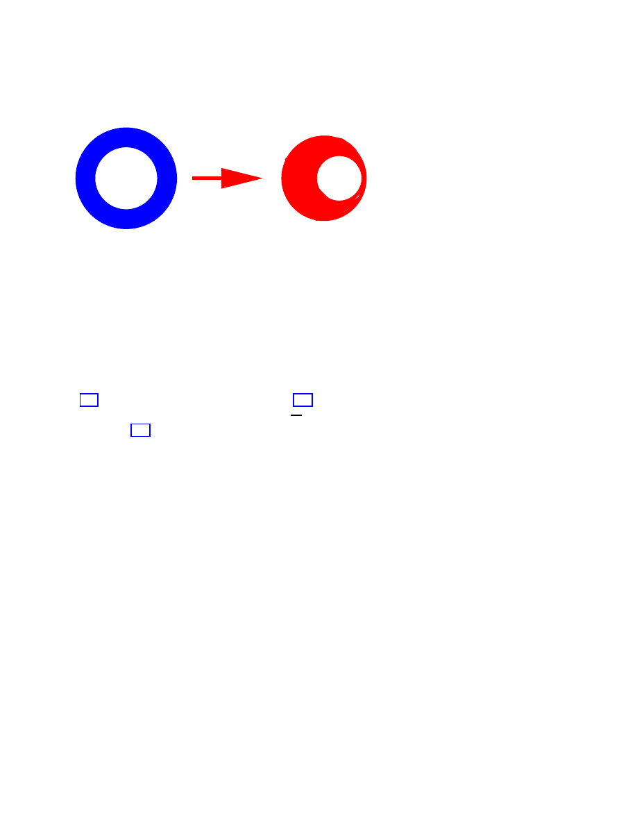
World−sheet Torus
Pinched Torus
Figure 5: Extra world-sheet partition function divergencies arising from pinched tori. Regu-
larizing such pinched surfaces modifies the β-function of the theory at lower genera, since it
introduces new types of σ-model counterterms. This is the essence of the Fischler-Susskind
mechanism.
where the suffix “old” denotes the right-hand-sides of the tree-level “graviton” equation in
(106), and that of the dilaton equation (107), and the prime denotes differentiation with
respect to the dilaton field Φ, δV
0
(Φ)
≡
δ
δΦ
δV (Φ).
From (136) we observe again that δc is a c-number (constant), as required by con-
sistency, for arbitrarty dilaton potential δV (Φ). In string-loop perturbation theory the
dilaton potential can be computed order by order, and has the generic form:
δV (Φ) =
X
n
≥1
a
n
e
(n+1)Φ
(137)
where we remind the reader that g
s
= e
Φ/2
is the string coupling constant, which is a
string-loop counting parameter, as explained in Lecture 1.
An important physical consequence of the presence of a dilaton potential due to string
loop corrections is the possibility of having De Sitter (inflationary) solutions in string
theory, i.e. solutions in which the Hubble parameter is constant in time H(t) = cons. This
implies an exponentially expanding Universe, with scale factor
a(t)
∼ e
Ht
(138)
The constancy of H can be achieved by selecting constant values for the dilaton and axion
fields φ
0
= const, b = b
0
= const, and non-trivial values for the dilaton potential, induced
by string loops:
R = 12H
2
= 2 [δV (Φ)
− δV
0
(Φ)] ,
δc =
−3δV
0
(Φ)e
−Φ
(139)
One should emphasize the crucial rˆole of the constant value of the dilaton field in deter-
mining both the value of the Hubble constant during the inflationary period of the string
Universe, and the string coupling g
s
= e
φ
0
/2
.
39
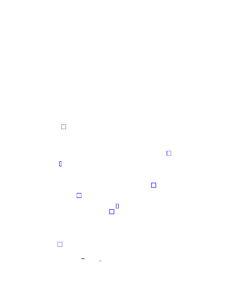
The physically interesting issue is how one can exit from the inflationary phase in
string Universes. In the simplified background considered above this cannot be possible in
a smooth continuous way. The rest of the lectures will be therefore devoted to a rather
brief, but to the point, discussion of more complicated string backgrounds and scenaria
that might achieve such a graceful exit from the inflationary period. We shall also point out
some essential problems that an eternal de Sitter Universe poses for critical string theory
in general, namely for a proper definition of scattering amplitudes which is an essential
feature of any critical string theory.
3.3
De Sitter Universes and pre-Big Bang scenaria: the crucial
rˆ
ole of the Dilaton Field
3.3.1
Life before the Big Bang in string theory?
As we have seen above, a non-trivial dilaton field Φ is an important ingredient for providing
inflationary, and in general expanding, Universes in string theory. As argued by Veneziano
and collaborators [11], the presence of a non-trivial dlaton potential may result in scenaria
for expanding Universes in which there is no initial singularity (Big Bang), since in such
cases the “singularity” is replaced by a (yet not fully known) non-perturbative strongly-
coupled region of string theory, in which g
s
= e
Φ/2
1. This is the so-called Pre Big-
Bang scenario (PBB) of the string Universe, which we now proceed to discuss in general
terms. For details we refer the interested reader in the relevant literature [11].
In PBB scenaria one is typically encountering the situation for a dilaton potential
depicted in figure 6. In generic PBB models the string Universe has a (weak string coupling)
“life”, before one reaches the “big bang”, which is not a singularity, but a potential barrier
separating the weak phase from that at which the string theory becomes strongly coupled.
The weakly coupled string-theory (pre Big Bang) region can be treated analytically by
means of Einstein-type low-energy effective actions, of the form (91). In this region one
considers homogeneous Bianchi type I solutions of the equations of motion obtained from
the string-effective action [11].
Let t = 0 be the “Big-Bang” time moment, i.e. the time moment for which the dilaton
potential has its maximum height (see figure 6). The pre Big Bang (weakly coupled)
solution occurs for t < 0, and has the form [11]:
ds
2
E
=
−(dt)
2
+
X
i
(
−t)
2a
i
dx
i
dx
j
η
ij
,
Φ =
−(1 −
X
i
a
i
)ln(
−t) ,
X
i
a
2
i
= 1 , t < 0
(140)
It is customary [11] to use a redefined dilaton field, shifted by the logarithm of the deter-
minant of the spatial part of the metric,
Φ
≡ Φ −
1
2
lndet(g
ij
) =
−ln(−t)
(141)
40
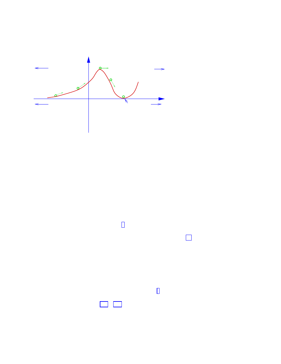
Φ
V(
)
0
0
Weak Coupling
Strong Coupling
Φ
Initial
Φ
Present
Φ
=
Φ
0
Figure 6: A typical dilaton potential encountered in pre-Big-Bang scenaria for string Uni-
verse. In such scenaria the initial (Big-Bang) singularity of standard cosmology is absent,
and is replaced by a non-perturbative region of string theory, in which the string coupling,
being given by the exponential of the dilaton field, is very strong. The arrows indicate
flow of cosmic time. The dilaton today is at (or close to) the minimum of its potential.
At present the rigorous derivation of such potentials from exact string theory models is
lacking
Notice that in PBB scenaria it is the early times regime that is characterized by a weakly
coupled string theory, and dilaton potential which asymptotes to zero. This has to be
contrasted with the situation in ref. [9], where it is the late times region which has these
features, as we have seen in the previous subsection.
Inhomogeneities are introduced in a straightforward manner [11]:
ds
2
E
=
−(dt)
2
+
X
b
e
b
i
(x)e
b
j
(x)(
−t)
2a
b
(x)
dx
i
dx
j
,
Φ =
−(1 −
X
i
a
i
)ln(
−t) ,
X
i
a
2
i
= 1 , t < 0
(142)
3.3.2
Stringy Dilaton Driven Inflation in PBB scenaria
In a PBB scenario, like the one depicted in figure 6, the dilaton continues to grow (as
time evolves) in such a way that the string coupling g
s
= e
Φ
becomes strong and, hence,
perturbative solutions like (140),(142) are no longer possible. In strong string coupling
situations the resummation of string world-sheet genera has to be performed, something
which at present is not feasible. Moreover, many physicists believe that in such strong
string-coupling situations even the concept of a σ-model breaks down, and one encounters
a fully non-perturbative stringy situation which is far from being understood at present. It
41
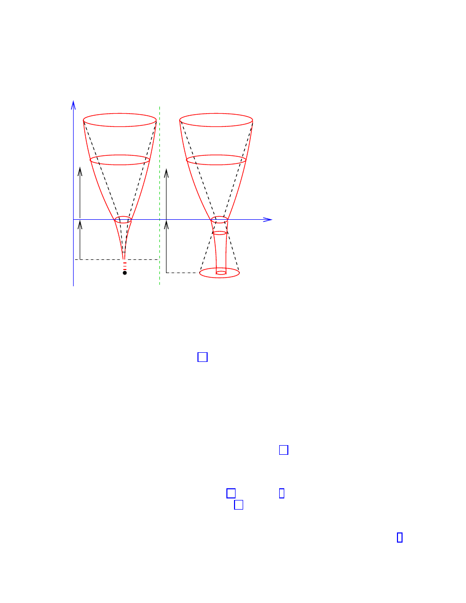
Space
Time
Now
Big Bang
Here
Here
Inflation
Post
Big Bang
expansion
Pre Big
Bang
Inflation
Start of
collapse/
inflation
normal
expansion
Figure 7: A typical space-time “wine glass” diagram for the PBB scenario (right figure),
and the corresponding diagram for conventional Big Bang Cosmology (left figure). The
eras of pre big bang life of the Universe and dilaton driven inflation, in the PBB scenario,
are indicated (original figure in ref. [11])
is in this regime that non-perturbative concepts like branes, M-theory etc., are applicable,
and one would hope to find appropriate dualities which would map the strongly-coupled
string theory to a dual theory which could be treated perturbatively in an analytic way.
At prsent, despite effort, this issue is still open in our opinion, and this prevents one from
providing analytic arguments in support of the crossing of the potential “Big-Bang” barrier.
However, the lack of analytic treatment does not prevent one from making a qualitative
description as to how the situation is expected to be [11]. After crossing the barrier
one expects to have an inflationary phase, driven by the dilaton field, and eventually a
graceful exit from it, so as to reach the present era of our power-law expanding Universe.
Schematically, the PBB scenario and its post big-bang inflationary phase is represented by
means of “wine-glass” space-time diagrams [11]. In figure 7, which is a crude reproduction
of the original figure suggested by Veneziano [11], the PBB scenario for a string Universe,
together with its post BB evolution, is compared, in terms of the corresponding space time
diagrams, with that of a standard Big-Bang Cosmology. A physical picture of what it is
envisaged in a PBB situation, including the dilaton-driven inflation is given in figure 8.
Our Universe starts as a small (Planckian) fluctuation of the string vacuum, and then turns
42
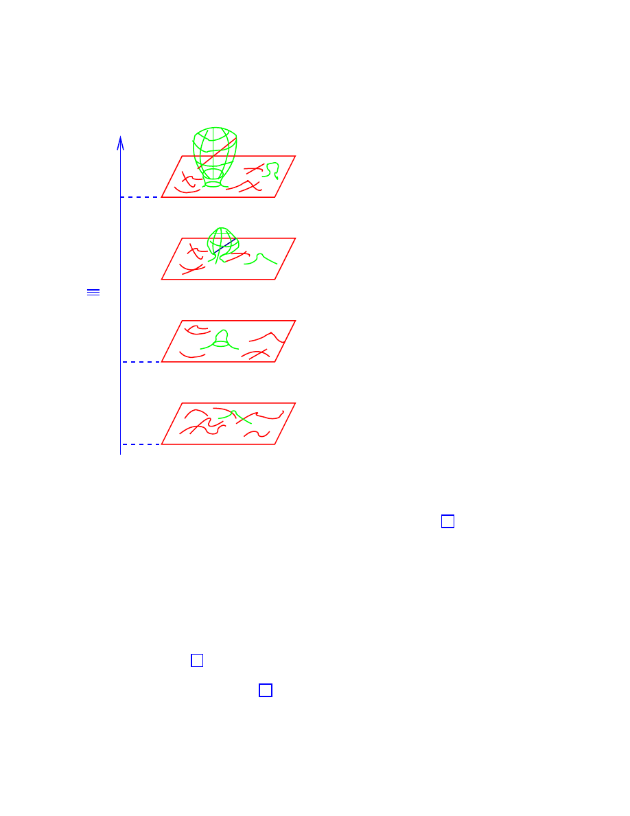
cm
10
−2
cm
10
−8
10
−13
cm
Weak
field
phase
t
i
Inflation
Collapse
Time
0
String &
Friedman
phases
Figure 8: A physical representation of the PBB dilaton-driven inflationary phase of the
string Universe. The figure is self explanatory (original figure in ref. [11]).
into a bubble that grows to enter the post Big-Bang era of normal Friedman expansion we
witness today. The creation of another bubble cannot be excluded in such scenaria. This
would bear similarities to stochastic inflationary scenaria. At present a rigorous derivation
of such a picture from specific string models is still far from being complete, at least in our
opinion.
Before closing this subsection it is worthy of pointing out that in the Einstein-frame
PBB scenaria the issue of dilaton-driven inflation becomes equivalent to that of studying
gravitational collapse [11], in the sense of the Einstein-metric spatial volume element being
shrunk to zero size at a certain moment, as time goes backwards. The reason is simple:
in this frame, one observes from (91) that the dynamics of the problem are those of a
minimally coupled scalar field Φ to Einstein gravity. Such a situation is characterized by
positive pressure, as can be trivially verified, and thus it cannot lead to inflation. However,
at these singularities the dilaton also blows up, and one can verify that in PBB scenaria
43
the stringy metric, related to the Einstein one via (90), also blows up there, leading to
stringy inflation. Such a situation is depicted in figs. 7, 8. For more details on such issues
in the context of PBB scenaria we refer the reader to the literature [11].
3.4
Some Phenomenological Implications of String Cosmology
The string cosmologies we have discussed so far have a far richer spectrum of physical
excitations, as compared with standard cosmologies. The quantum fluctuations of these
stringy excitations are expected to undergo amplification under inflation, which is expected
to lead to a rich unconventional phenomenlogy, not characterizing the case of conventional
cosmologies.
In PBB scenaria one can actually show [11] that some “pump” fields, a terminology
to be defined immediately below, tend to grow during the PBB inflation in contrast to
the situation encountered in standard (conventional, field-theoretic) inflationary scenaria,
where they tend to decay.
Consider a generic perturbation Ψ in the low-energy limit of string theory with action
(86) in the σ-model frame (e.g. metric, dilaton, axion fluctuation etc). We assume the
theory has been appropriately compactified to four space-time dimensions. As mentioned
previously, in the context of our generic discussion in this lectures, we shall not bother
with explicit details of the internal dimensions. The effective action of this perturbation
has the generic form:
I
eff,pert
=
Z
dηd
3
xs(η)
h
Ψ
02
− (∇Ψ)
2
i
(143)
where η is the conformal time, defined by dη = dt/a(t), with a(t) the scale factor of the
Universe (in the σ-model frame), and the prime denotes differentiation with repsect to
η, ∂/∂η. The function s(η) is a function of the scale factor a(η) and other scalar fields
(dilaton, moduli-i.e. fields related to the internal dimensions etc), which characterize the
string background under consideration. The function s(η) is called a “pump” field, since
a s(η)
6= const couples non-trivially to the perturbation Ψ and leads to the production of
pairs of quanta of this perturbation.
The pump fields are crucial in determining the evolution of the perturbation. Let Ψ
~k
be a Fourier component of such a perturbation. Then one may define:
b
Ψ
~k
≡ s
1/2
(η)Ψ
~k
,
which can be shown to satisfy a Sch¨odinger type equation [11]:
b
Ψ
00
~k
+
h
k
2
− (s
1/2
)
00
s
−1/2
i
b
Ψ
~k
= 0
(144)
where the prime denotes differentiation w.r.t. the conformal time η.
In string cosmology, and in particular PBB scenaria, the most interesting perturbations
correspond to the following pump fields [11]:
Gravity waves, dilaton :
s(η) = a
2
e
−Φ
,
Heterotic gauge bosons :
s(η) = e
−Φ
,
B
µν
Kalb
− Ramond field, (axion) :
s(η) = a
−2
e
−Φ
.
(145)
44
where a is the RW scale factor in the σ-model frame, related to the scale factor in the
Einstein frame a
E
by a
E
= ae
−Φ/2
. These are found easily by looking at the corresponding
terms of the low-energy string effective action (in these lectures we only exhibited explicitly
the gravitational part of the effective action (86), (91) (or (108)), and not the gauge and
other parts. The interested reader is referred to the literature for explicit forms of such
background fields [1]). For example, looking at the axion term in the Einstein frame
effective action (108) it is immediate to see that the axion b perturbations will have a
pump field a
2
e
Φ
. On the other hand, when expressed in terms of the field strength of
the Kalb-Ramond field B
M N
, H
µνρ
= e
2Φ
µνρλ
∂
λ
b, such axion terms lead to effective action
H-terms of the form (91), and therefore to the Kalb-Ramond pump field indicated in (145).
After amplification during PBB inflation, such perturbations may lead to observable
effects. Below we shall briefly catalogue the claimed effects. The interested reader may
find more detailed discussion in the literature [11].
• Tensor Perturbations: such perturbations are associated with gravitational field per-
turbations, and may have effects in the observable cosmic gravitational radiation
background (gravity waves). Such effects are though extremely tiny, due to the
weakness of the itneraction. Conventional models of inflation also have such pertur-
bations, and it will be very difficult to disentangle the stringy situations from the
conventional ones, as far as tensor perturbations are concerned, even if the gravita-
tional radiation is observed.
• Dilaton Perturbations: since the dilaton plays the rˆole of the inflaton in string cos-
mology, as it drives string inflation, as discussed above, it is the natural source for
adiabatic scalar perturbations. One would expect it to lead quite naturally to a
quasi scale invariant Harrison-Zeldovich spectrum of adiabatic perturbations. This
would be desirable in explaining the observed cosmic microwave bacground (CMB)
anisotropies. Unfortunately, however, detailed studies in the PBB scenaria [11] have
revealed that both scalar and tensor perturbations remain exceedingly small at large
scales, so CMB data cannot be explained by the dilaton inflation-amplified pertur-
bations.
• Gauge-Field Perturbations: in standard cosmology there is no amplification of vac-
uum fluctuations of gauge fields. This is due to the fact that the inflaton in such cases
makes the metric conformally flat, and in such metrics, the gauge fields decouple from
geometry in D = 3 + 1 dimensions. In contrast, in PBB stringy scenaria, the effective
gauge coupling, being related proportionally to the string coupling g
s
= e
Φ/2
, grows
together with the inflated space. This is an exclusive feature of stringy models. In
this sense, one would expect [11] that PBB, or in general stringy inflationary scenaria,
could provide an explanation for the origin of primordial seeds of the observed galac-
tic magnetic fields. This, however, still remains a theoretically unsolved problem.
Gauge perturbations interact considerably with the hot plasma of the early post big
Bang Universe, and hence covnerting the primordial seeds into those that may have
existed in the era of galaxy formation is a non-trivial and still unresolved task.
45
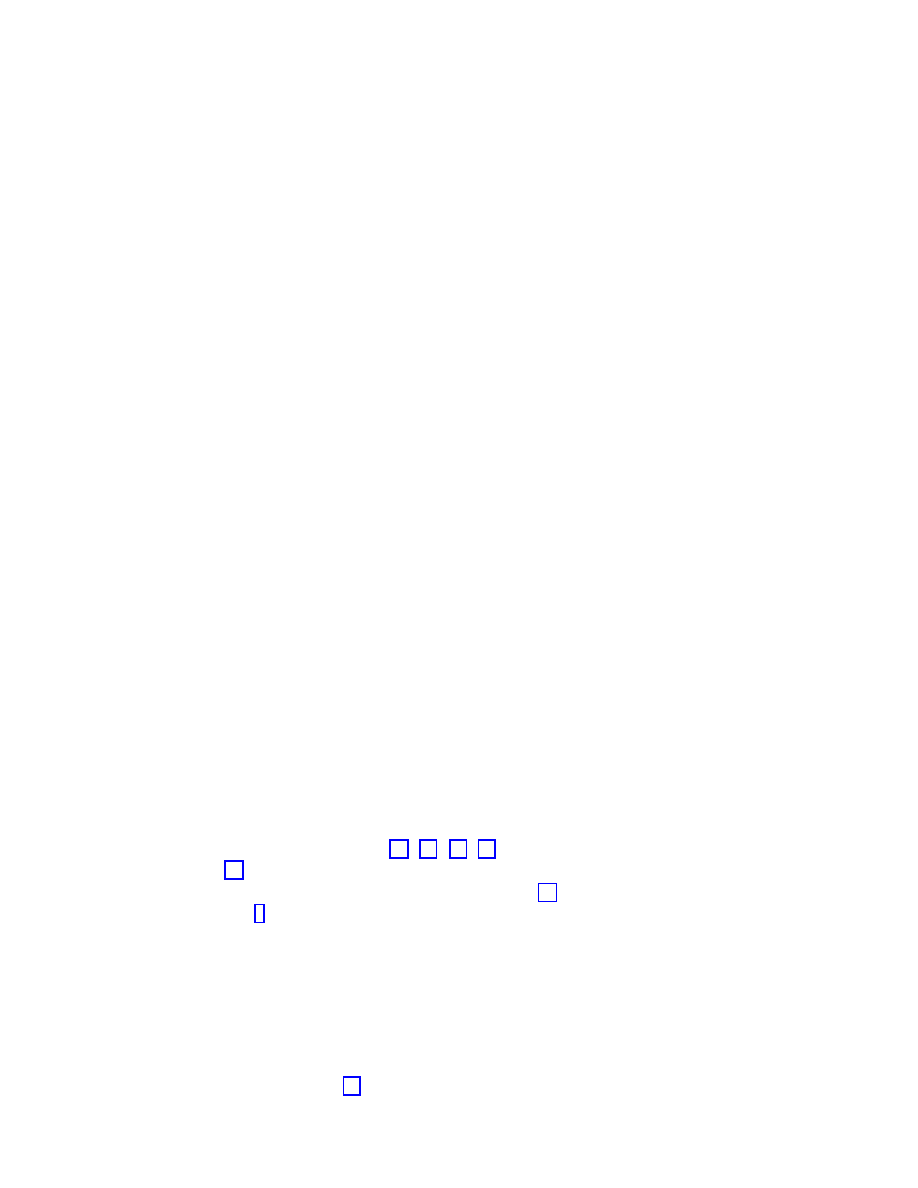
• Axion Perturbations: As we have discussed above, in four space-time dimensions,
the field strength of the antisymmetric tensor field of the σ-model is related to the
axion field b: H
µνρ
= e
2Φ
µνρλ
∂
λ
b. It must be stressed that the spectrum of the axion
field perturbations is very sensitive to the cosmological behaviour of the internal
(compactified) dimensions during the string inflationary era, thereby making axions
a window to extra dimensions. On the other hand, the axion spectrum is flat even
red (tilted towards large scales).
With these brief comments we finish our discussion on the string cosmological scenaria.
We only glazed the surface of a huge subject here, and the interested reader is strongly
advised to seek further details in the literature. As we have seen, there are many issues
that need further exploration, both theoretical and experimental ones. There are important
differences from standard cosmology. However, de Sitter Universes in string theory pose
serious theoretical challenges as well, which we did not discuss so far. This, and ways of
incorporating such backgrounds in a mathematically consistent string-theory framework,
will be the (speculative) topic of the third Lecture, which we now turn to.
4
Lecture 3: Challenges in String Cosmology and
Speculations on their Treatment
4.1
Exit from Inflationary Phase: a theoretical challenge for
String Theory
An important, and still unresolved issue, in stringy inflationary cosmology is the graceful
exit from the De Sitter (inflation) phase. As we have seen previously, an important in-
gredient for inflation is the existence of a dilaton potential, which in critical (conformal)
string theories is absent at tree world-sheet level, and can only be generated by resum-
ming string loops (higher genera). In PBB scenaria, during the inflationary period one is
dealing with a strongly coupled phase of string theory, and hence analytic arguments on
such a resummation cannot be provided. Exit mechanisms have been proposed though at
a qualitative level by many groups [11, 12, 13, 14]; some of them involve non-local dila-
ton potentials [13], which however lack a good motivation within the framework of string
theory; others impliment exit via quantum tunnelling [14] through the dilaton potential
barrier (see figure 6), which exploits the associated Wheeler-de-Witt equation, without
modification of the low-energy string effective actions. Unfortunately, although in such
tunnelling scenaria the quantum probability of a classically forbidden exit turns out to
be suppressed by e
−Φ
factor, and a priori looks to be a promising scenario, however this
suppression exist throughout the three-space, and thus in such scenaria only tiny regions
have a reasonable chance of tunnelling.
Exit from inflationary phase is a generic challenge for critical string theory, not only
of PBB scenaria. This problem becomes even more serious today, where there seems
to be experimental evidence [15] (from high-redshift supernovae Ia data, supported by
46
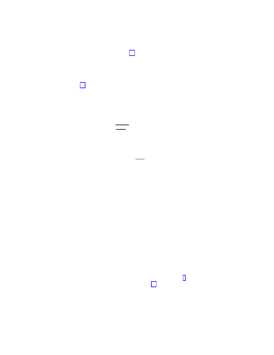
complementary observations of CMB data [16]) that our Universe today is in an accelerating
phase, ¨
a(t) > 0, which, within the Friedman cosmological model, implies also a non-trivial
positive cosmological constant Λ > 0. In fact there is evidence that 70% of the total
available energy density is dark energy component, not matter, which could be an honest
cosmological constant, or, even, a relaxing to zero time-dependent energy component of
a quintessence field [17]. This may be said differently: our Universe is still in a de Sitter
phase, which if true may imply eternal acceleration, given that in such a phase, with a non-
zero positive cosmological constant, eventually the vacuum energy due to Λ will become
dominant over the matter, whose density decays with the scale factor as a(t)
−3
. In such
a vacuum-dominated Universe, the scale factor of a Friedman model varies exponentially
with the Robertson-Walker time t:
a(t)
∼ e
q
8πGN
3
Λt
,
Λ = const > 0
(146)
Such eternally accelerating Universes are plagued by the presence of finite cosmic horizons
δ
H
:
δ
H
∝
Z
∞
t
0
dt
a(t)
<
∞
(147)
If the Universe does not exit from the inflationary (de Sitter) phase, then the inevitable
existence of horizons will imply the impossibility of defining properly asymptotic states , and
hence a scattering matrix S = e
−iHt
, where H the Hamiltonian operator of the Universe.
The situation is somewhat analogous to that of having space-time boundaries, e.g.
due to the existence of microscopic black hole fluctuations in certain scenaria of quantum
gravity. There is “information” loss in such a situation for asymptotic observers, due to
modes crossing these boundaries, which implies that an asymptotic observer cannot define
pure quantum states
|ψi, but only mixed states, defined by a density matrix ρ = Tr
M
|ψihψ|,
obtained by tracing over unobserved degrees of freedom
{M}.
We recall that in a unitary quantum theory, the S-matrix connects asymptotic in states
to asymptotic out states:
|outi = S |ini
(148)
On the other hand, if one encouters mixed states, as is the case of open quantum me-
chanical systems, non-equilibrium systems, or systems with space time boundaries, such
as gravitational theories with local or global (cosmological) horizons, then the concepts
of “in” and “out states” should be replaced by those of “in” and “out density matrices”,
given that pure states evolve to mixed ones, as depicted in figure 9.
In such a case, as suggested first by Hawking [18], one can still link the in and out
density matrices using not the S-matrix, but another object, called /S matrix:
ρ
out
= /Sρ
in
(149)
The operator /S factorizes into a product SS
†
only in pure state quantum mechanics without
unobserved degrees of freedom, in which ρ =
|ψihψ|. In general, however, once there are
47
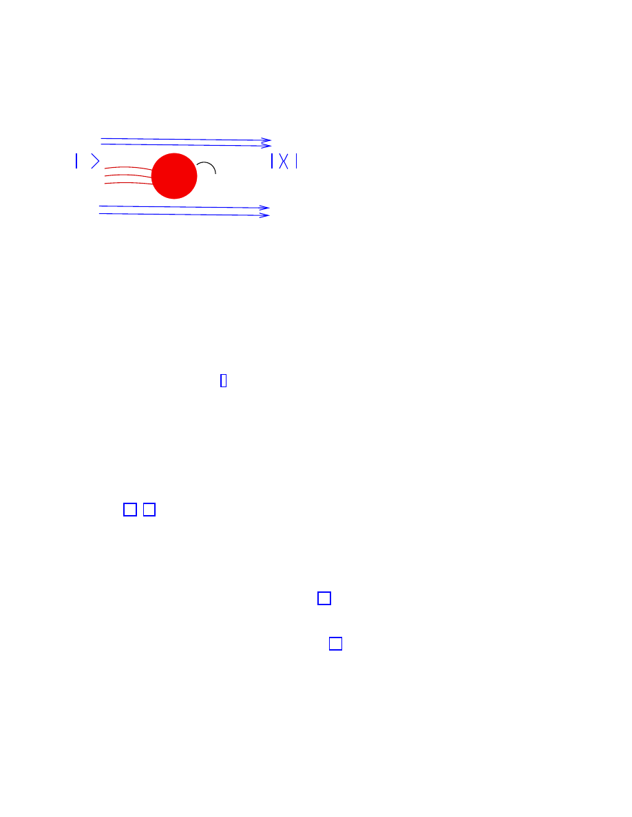
ψ ψ
Tr
ρ =
ψ
IN
OUT
ξ
,ψ
ξ
ψ
modes
modes
ψ
modes
ξ
Horizon
(mixed)
(pure)
Figure 9: Evolution of pure quantum mechanical states to mixed ones in the presence of
a space-time boundary. An asymptotic future observer O
0
has to trace over modes ξ that
cross the horizon, and hence are unobserved by him/her. The situation is common for
both local(black hole) and global (cosmic) horizon boundaries.
unobserved degrees of freedm, thereby opening up the system, as is the case of horizons
(local or global) (see figure 9), the factorization property of /S is lost:
/S
6= S S
†
(150)
In such systems one cannot define on-shell scattering amplitudes.
This is a serious theoretical challenge for string theory. As we have discussed in Lec-
ture 1, string theory is by construction a theory of on-shell S-matrix, based on scatter-
ing amplitudes which are reproduced by the appropriate conformal invariance conditions.
Thus, de-Sitter Universes (with eternal acceleration) pose a challenge which needs to be
resolved [19, 20].
In the remaining of these lectures I shall present some speculations as to how this
problem can be tackled. A straightforward possibility would be to demonstrate the exis-
tence of string backgrounds which allow graceful exit both from the de-Sitter as well as
the accelerating phases. Within critical (conformal) string theory such a scenario has not
yet been achieved. However, I will discuss an alternative possibility to such critical string
theory models, known as Liouville Strings [21], , where graceful exit may be a realistic
possibility. Such string theories are supposed to be mathematically consistent attempts to
formulate σ-models away from their world-sheet renormalization-group fixed (conformal)
points, i.e. σ-models for which the conditions (64) are not valid. The topic, however, is
by no means as well established as critical strings, and therefore the treatment requires
extreme caution. Nevertheless, as I will try to argue in this part of the Lectures, Liou-
ville strings have some nice and quite interesting features which certainly support further
studies and are worthy of discussion.
48
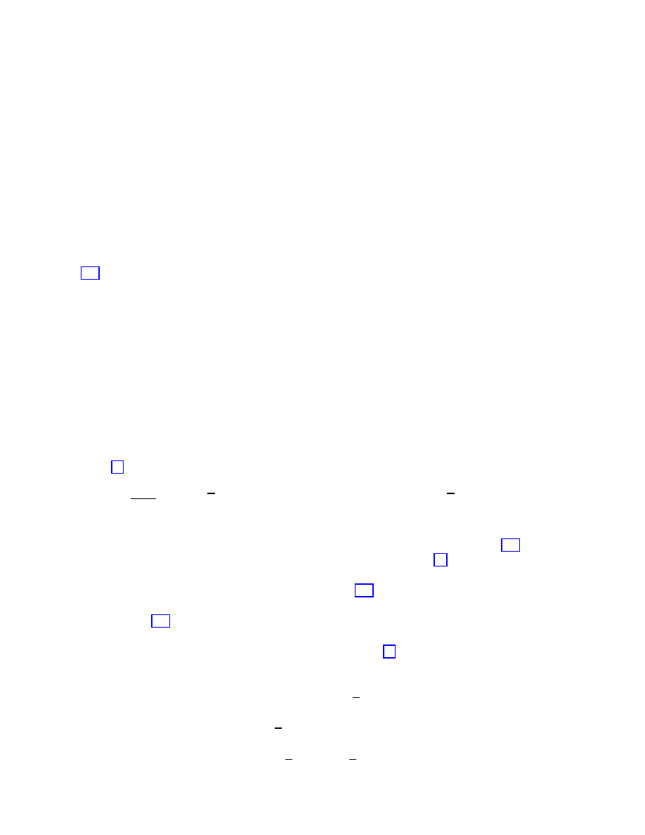
4.2
Cosmological Backgrounds in String Theory and World-Sheet
Renormalization-Group Flow
We shall introduce the reader into the topic of Liouville strings by first elaborating fur-
ther on time-dependent (cosmological) backgrounds of the σ-model theory. Consider for
definiteness a (d + 1)-dimensional target space time σ-model, describing propagation of a
Bosonic closed string on a background consisting of the massless string multiplet of gravi-
ton g
M N
(~x, t), antisymmetric tensor B
M N
(~x, t) and dilaton Φ(~x, t) fields. Here ~x span a
d-dimensional Euclidean space (x
i
, i = 1, . . . d) and t is the time. Assume the (d + 1)-
dimensional σ-model at its conformal point, at which the conformal invariance conditions
(154) are satisfied.
Target-space diffeomorphism invariance and the Abelian gauge symmetry associated
with B
M N
, discussed in Lecture 1, can be used to ensure:
B
0i
= 0 ,
G
00
=
−1 ,
G
0i
= 0 ,
i = 1, . . . d
(151)
A (d + 1)-dimensional string solution can be represented as a trajectory f
A
(t) in the
space of d-dimensional σ-model fields x
i
, with the time t being a parameter along the
trajectory:
f
A
=
{g
ij
(~x(t)), B
ij
(~x(t)), Φ(~x(t))
} , i, j = 1, . . . d
(152)
[NB5: in this section we shall use the notation M, N, . . . for (d+1)-dimensional spacetimes,
and i, j . . . for d-dimensional space ]
The set of fields f
A
can be viewed as couplings of a σ-model in d-dimensional target
space [22]
S
σ
=
1
4πα
0
Z
d
2
σ
h
√
γg
ij
(~x)∂
α
x
i
∂
α
x
j
+ i
αβ
B
ij
(~x)∂
α
x
i
∂
β
x
j
+ α
0
√
γR
(2)
Φ(~x)
i
(153)
As we shall discuss now, the orbits f
A
resemble standard world sheet renormalization group
(RG) trajectories in the space of couplings g
i
of the two-dimensional theory (153). This
is a very important feature which goes beyond a simple analogy [23], as we shall discuss
later on in the lectures.
For the moment we note that the string theory 153) lives necessarily in a non-critical
dimension, since the (d + 1)-dimensional theory has been assumed critical. Thus, the
couplings of (153) lie away from their fixed point, and hence must have non-trivial RG
flows (and therfore non-trivial Weyl anomaly coefficients). Their flows are to be identified
with the flow in the real time t, as we shall discuss now [23].
Consider the
O(α
0
)
b
β-functions of the d-dimensional σ-model theory:
b
β
g(d)
ij
= α
0
R
ij
+ 2
∇
i
∂
j
Φ
−
1
4
H
imn
H
mn
j
,
b
β
B(d)
ij
= α
0
−
1
2
∇
m
H
m
ij
+ H
m
ij
∂
m
Φ
,
˜
b
β
Φ(d)
= β
Φ(d)
−
1
4
g
ij
b
β
g(d)
ij
=
1
6
h
c
(d)
(~x)
− 26
i
,
49
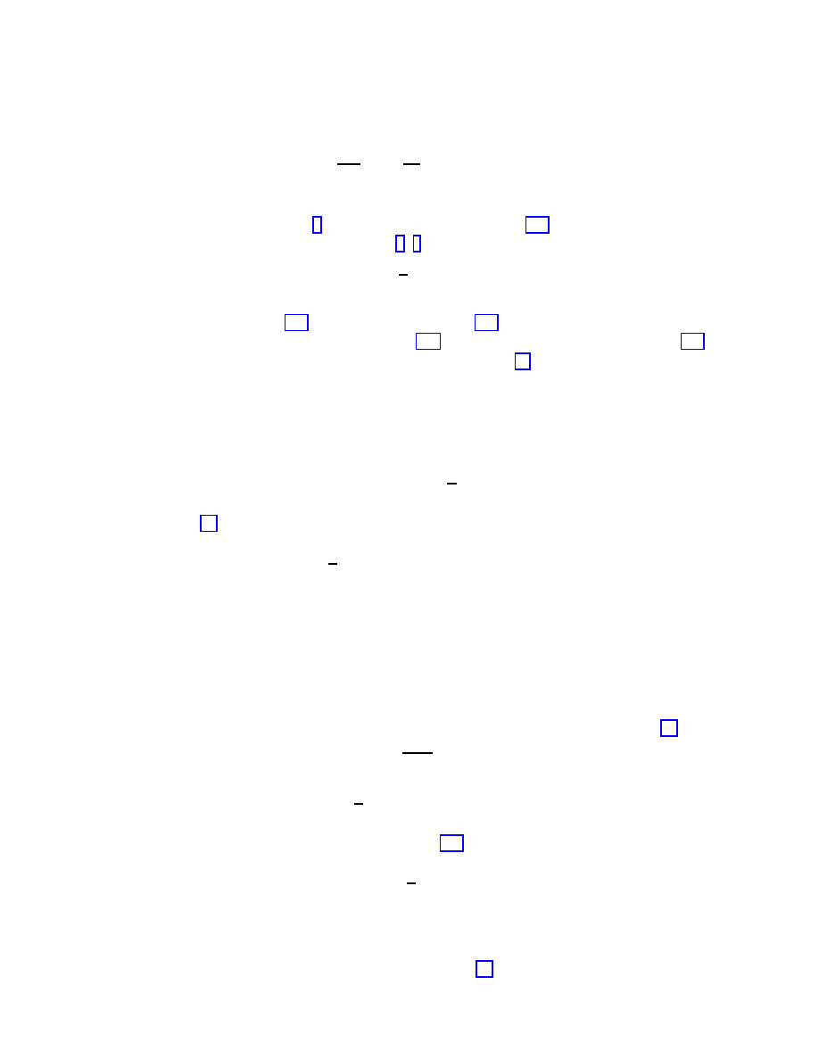
c
(d)
(~x) = d
−
3α
0
2
R
−
1
12
H
2
− 4(∇Φ)
2
+ 4
∇
2
Φ
(154)
Above the superscript (d) denotes d-dimensional quantities, and c
(d)
(~x) is the Zamolod-
chikov running central charge [3] of the non-critical theiory (153). This determines the
d-dimensional target-space effective action [4, 6]:
I
(d)
eff,off
−shell
=
Z
d
d
x
√
ge
−2Φ(~x)
h
c
(d)
(~x)
− 26
i
(155)
The off-shell variations of (155) yield the
b
β-functions (154). It must be stressed that the
non-criticality of the d-dimensional σ-model (153) implies that the
b
β-functions in (154)
are non-vanishing (so the conformal invariance conditions (64) are not satisfied for the
d-dimensional theory).
Let us now consider the corresponding (d + 1)-dimensional
b
β
i
, which should be set to
zero, on account of the criticality assumption of the (d + 1)-dimensional theory. Let us
then split the equations into temporal and spatial (d-dimensional) parts. The result is
facilitated if one uses a shifted dilaton:
ϕ
≡ 2Φ − ln
√
g
(156)
Then we have [22]:
0 =
b
β
g(d+1)
00
= 2 ¨
ϕ
−
1
2
g
ik
G
j`
˙g
ij
˙g
k`
+ ˙
B
ij
˙
B
k`
,
0 =
b
β
g(d+1)
ij
=
b
β
g(d)
ij
− g
00
h
¨
g
ij
− ˙ϕ ˙g
ij
− g
mn
˙g
im
˙g
jn
− ˙
B
im
˙
B
jn
i
,
0 =
b
β
B(d+1)
ij
=
b
β
B(d)
ij
− g
00
¨
B
ij
− ˙ϕ ˙
B
ij
− 2g
k`
˙g
k[i
˙
B
j]`
,
0 = c
(d+1)
− 26 = c
(d)
− 25 − 3g
00
¨
ϕ
− ( ˙ϕ)
2
(157)
where the superscript (d+1) denotes critical dimension d+1 = 26 Bosonic string quantities,
and the indices 0 denote temporal compontents.
It is straightforward to show that these equations are derived from the action [22]:
I
(d+1)
eff
=
Z
dtd
d
x
q
|g
00
|e
−ϕ
c
(d)
(~x)
− 25+
3g
00
˙
ϕ
2
−
1
4
g
ik
g
j`
( ˙g
ij
˙g
k`
+ ˙
B
ij
˙
B
k`
)
(158)
In adition, one also should satisfy the conditions (151), which imply the constraints:
0 = β
g(d+1)
0i
=
∇
k
g
k`
˙g
`i
−
1
2
˙
B
k`
H
k`
i
+ 2∂
i
˙
ϕ
− g
k`
˙g
`i
∂
k
ϕ ,
0 = β
B(d+1)
0i
=
−g
ik
∂
j
g
k`
g
jn
˙
B
n`
+ 2 ˙
B
ij
∂
j
ϕ
(159)
which, to
O(α
0
), can be shown not to have any important consequences other than restrict-
ing the initial values of the fields and their derivatives [22].
50
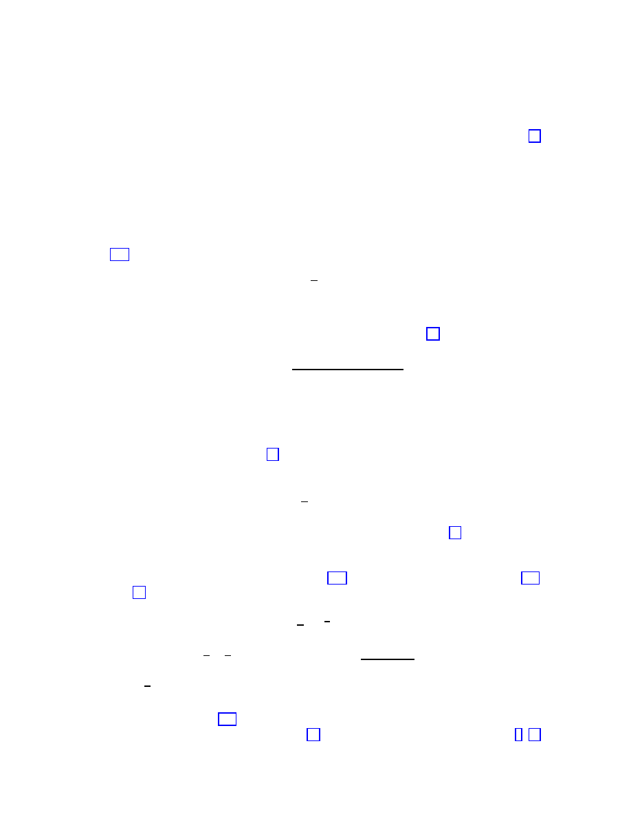
To proceed with our cosmological solutions one should define quantities integrated over
spatial coordinates ~x, which thus have only a time dependence. In this spirit we define [22]:
ϕ
0
(t)
≡ −ln
Z
d
d
xe
−ϕ(~x,t)
(160)
This allows a splitting of the dilaton field ϕ(~x, t) into ~x-dependent and ~x-independent parts:
ϕ(~x, t) = ϕ
0
(t) + ˜
ϕ(~x, t)
(161)
From (156), then, we have:
ϕ
0
(t) =
−ln
Z
d
d
x
√
ge
−2Φ(~x,t)
≡ −lnV
(d)
(162)
where V
(d)
is the proper volume of the d-dimensional space.
One can also define the space-aveage of a function f (~x, . . .) as [22]:
hhf(~x, . . .ii =
R
d
d
xf (~x, . . .)e
−ϕ(~x,...)
R
d
d
xe
−ϕ(~x,...)
(163)
From this we observe that
˙
ϕ
0
(t)
≡ −Q(t) = hh ˙ϕ(~x, t)ii
(164)
The time-dependent function Q(t) is related to the central charge deficit, and hence to the
Q of the linear dilaton background (95), of Lecture 2, as follows: At the “fixed points” of
the t-flow: ˙g
ij
= ˙
B
ij
= ¨
ϕ = ¨
Φ = 0, it follows that Q = Q
0
=constant, and in fact:
ϕ
0
(t) =
−
1
2
Q
0
t + const
(165)
which is a linear dilaton background, analogous to that examined in (95), corresponding
to conformal field theory models with central-charge deficits Q
0
.
In general, however, away from the “fixed-pointas” of the t-flow, Q(t) is a function of
t. Integrating the dilaton equation in (last of) (157), and taking the space average (163),
we obtain [22]:
˙
Q(t) + Q
2
(t) =
−
1
3
g
00
(c
− 25) ,
c = c(g, B, ϕ)
≡ hhc
(d)
(~x)
ii =
I
(d)
eff,off
−shell
V
(d)
+ 26
(166)
The function c plays the rˆole of the ‘running central charge’ of a non-conformal world-sheet
field theory away from the fixed points, in the presence of non-constant dilatons. Notice
that in case ˙
Q = 0 then (166) becomes just the definition of the central charge deficit
appearing in the linear dilaton background (95), or in standard non-critical strings [9, 21].
51
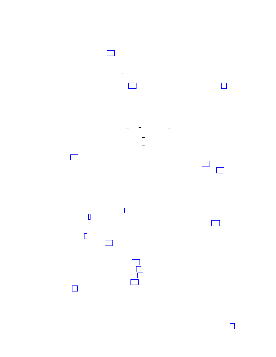
Using the first of equations (157) one may compute ˙
Q:
˙
Q(t) =
hh− ¨
ϕ + ˙
ϕ
2
− Q
2
ii = hh( ˙ϕ − hh ˙ϕii)
2
− ¨
ϕ
ii =
hh( ˙ϕ − hh ˙ϕii)
2
−
1
4
g
ik
g
j`
( ˙g
ij
˙g
k`
+ ˙
B
ij
˙
B
k`
)
ii
(167)
We also notice that the first three of (157) can be written in a compact form [22]:
¨
~g + Q(t) ˙~g = g
00
b
~
β
~
g
+
O( ˙~g
2
) ,
~g =
{g
ij
(~x) , B
ij
(~x)
} ,
(168)
with
Q
2
(t) =
−
1
3
g
00
[c(~g)
− 25] +
1
4
˙~g
2
,
g
00
=
−1
if
c(~g) > 25 ,
g
00
= +1
if
c(~g) < 25 .
(169)
The equations (168) are sufficient to describe the theory in the vicinity of fixed-points
(with respect to the t-flow) in the space of couplings
{~g} of the σ-model (153). Notice the
“friction” form of these equations, due to the presence of a non-trivial dilaton (164).
4.3
Liouville Strings and Time as a world-sheet RG flow param-
eter
The similarity of the t-flow with the two-dimensional renormalization-group flow is more
than a mere analogy, and if made [23], it results in some important consequences for
the underlying physics
. In that case, i.e. after identifying the target time t with a
renormalization-group flow parameter on the world sheet of the σ-model (153), the t-
dependence of Q(t) is identified with the RG scale dependence of the running Zamolod-
chikov central charge [3] of this two-dimensional non-conformal theory.
Notice that the equations (168) refer to couplings of a non-conformal σ-model, in a
d-dimensional target space, which however can become conformal in one target-space di-
mension higher, i.e. by making the trajectory parameter t a fully-fledged quantum field in
the σ-model. In this sense, the equations (168) may be thought of as a generalization of
the conformal invariance conditions
b
β
i
= 0 (64) of a critical (fixed point) theory. This is
precisely the principle of Liouville Strings [21].
From this point of view the equations (168) stem from the following fact: As just said,
Liouville theory [21] restores conformal invariance of σ-models which are away from their
fixed points, by coupling them with an extra fully fledged world-sheet quantum field ρ(σ, τ ),
the Liouville mode. If a vertex deformation V
i
is not a conformal (marginal) operator of
the σ-model, then the“Liouville-dressed” operator :
V
L
i
≡ e
α
i
ρ(σ,τ )
V
i
(170)
4
It should be stressed, though, that this is not the interpretation adopted by the authors of ref. [22].
52
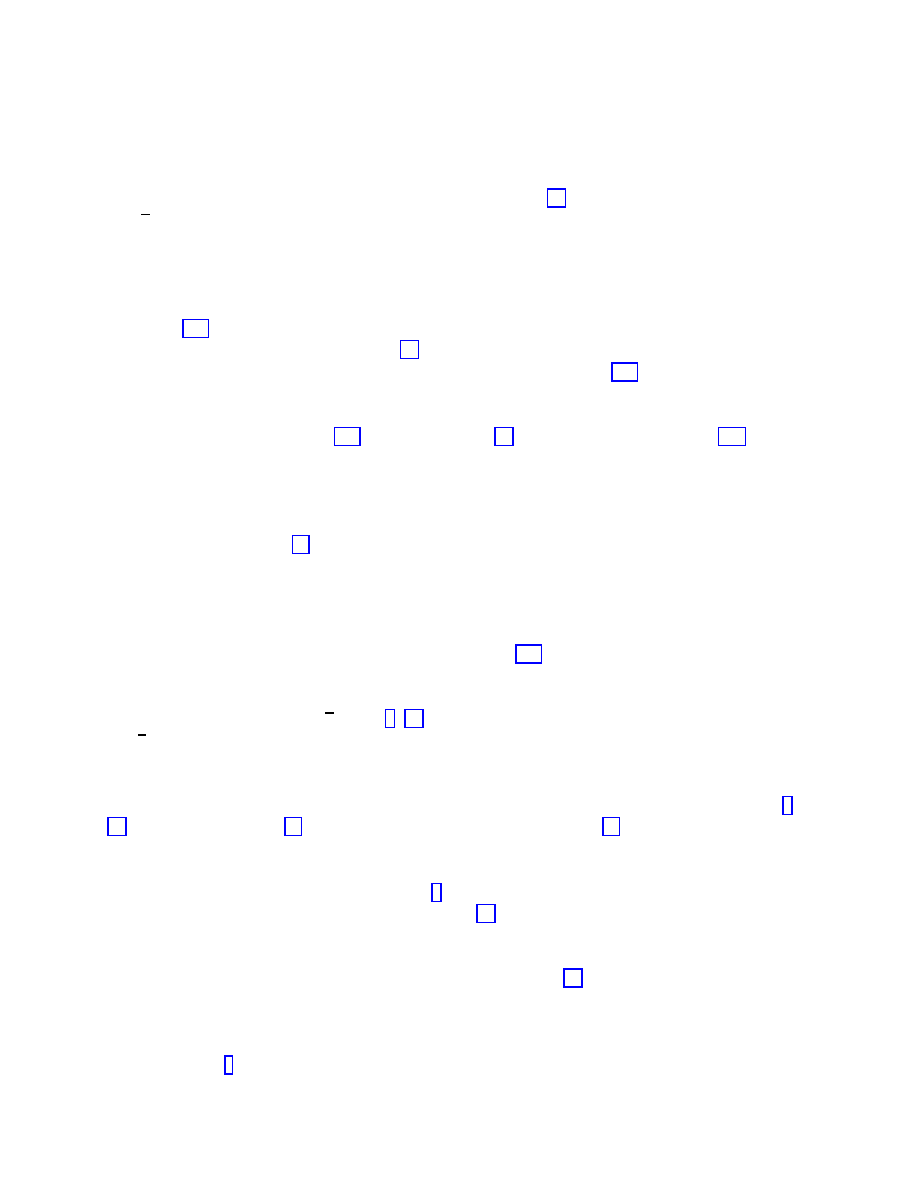
is a marginal operator, in the two-dimensional renormalization group sense. The quantity
α
i
is known as the ‘gravitational anomalous dimension’ [21], and it satisfies the equation
(for c
≥ 25 we are interested in here):
α
i
(α
i
+ Q) = ∆
i
no sum over i
(171)
where Q is a ‘charge at infinity’, with Q
2
denoting the central charge deficit, and ∆
i
= h
i
−2
is the anomalous dimension of the operator V
i
, with h
i
its conformal dimension. We repeat
that eq. (171) is nothing other than the condition that the Liouville dressed operator V
L
i
have vanishing anomalous dimension [21].
Consider, now, a Liouville-dressed deformation of the σ-model (170). The gravitationally-
renormalized couplings can be read off directly from this expression as: g
i
L
≡ g
i
e
α
i
ρ
. Con-
sidering the second derivative of g
i
L
with respect to the world-sheet zero mode of the
Liouville field, ρ
0
, and using (171), one can arrive [23] at equations of the form (168), with
the overdot denoting differentiation with respect to ρ
0
. In such equations the
O( ˙g
2
) terms
stem from possible ρ
0
dependence of Q, as in our case.
The Liouville mode ρ(σ, τ ) is nothing other than a dynamical σ-model field mode,
which appears in the sum over geometries of a non-conformal σ-model through, e.g. the
conformal gauge fixing (14). In a conformal field theory the Liouville mode decouples from
the world-sheet path integral. This is not the case, however, in a non-conformal σ-model,
and this is what we demonstrated above with our simplified example of stringy cosmology.
In such non-conformal cases, the Liouville mode becomes a fully fledged σ-model field in
order to restore the lost conformal invariance of the σ-model. From a physical point of
view the reader’s attention is drawn to the property (169) of the central charge deficit in a
Liouville theory. As we have seen above, the (d + 1)-dimensional target-space time (after
taking into account the Liouville field as a time coordinate) has a Minkowskian signature
for supercritical strings, i.e. c > 25 [9, 23], and Euclidean signature for subcritical strings,
i.e. c < 25.
In other words, the above-described “Liouville dressing” procedure implies a temporal
signature for the Liouville field, which can thus be identified with the time t, only in the case
where the central-charge deficit of the non-conformal σ-model theory is supercritical [9,
23]. By construction (14), the Liouville mode may be viewed [23] as a local world-sheet
renormalization-group scale, since it enters the expression of a covariant cutoff distance in
space, necessary for regulating ultraviolet divergencies in curved space in a way compatible
with two-dimensional general covariance [6]. The target-time then is nothing other than
the world-sheet zero mode of the Liouville field [23].
In this interpretation of target time as a world-sheet renormalization group scale there
is hidden an important property, which makes the Liouville coordinate different from the
rest of σ-model coordinates. That of its irreversibility [23]. This stems from the fact
that a world-sheet RG flow encodes information loss due to the presence of an ultraviolate
cutoff in the theory, and as such is irreversible. This irreversbility can be expressed in
terms of the irreversibility of the flow of the running central charge of the non-conformal
cut-off theory [3] (Zamolodchikov’s c-theorem), ˙c
≤ 0 towards a non-trivial infrared fixed
point. We shall come back to this important point later on.
53
Notice that the central charge has been argued to count physical target-space degrees of
freedom in the case of a stringy σ-model [24], and hence its decrease along a RG trajectory
is in perfect agreement with the loss of degrees of freedom in a cosmological situation with
horizons as the time (RG scale) evolves. It is for this reason that Liouville strings with the
time identified with a world-sheet RG scale are viewed as sort of non-equilibrium string
theories, with the conformal strings corresponding to equilibrium points [23]. What we shall
do in the remainder of the lecture, then, is to discuss some important physical features of
Liouville strings, such as time-dependent vacuum energy for the Liouville Universe, as well
as the impossibility of defining a proper on-shell scattering matrix for a Liouville string.
We shall also revisit the de Sitter string Universes from this point of view, and present
various possibilities for a graceful exit from the de Sitter, or in general, the accelerating
phase in the context of string theory.
4.4
Liouville String Universe and time-dependent Vacuum En-
ergy
The presence of a time dependent central charge deficit Q(t) in Liouville strings on cosmo-
logical backgrounds, with the time identified with the world-sheet RG scale [23], implies
- from the point of view of the corresponding effective target-space action (158)- a time-
dependent dilaton pontential, already at tree level world-sheet topologies [23]:
I
(d+1)
eff
3
Z
dtd
d
x
q
g(~x, t)e
−2Φ(~x,t)
h
−g
00
Q
2
(t)
i
(172)
One should compare this term with the corresponding term (108) of the model of [9] (after
appropriate metric redefinitions to go to the Einstein frame). In that case, δc came from
the internal conformal field theory (Wess-Zumino model), and this is why it turned out to
be constant. In contrast, in (172), which represents a more general situation, the deficit
depends on the RG scale t, since the underlying σ-model theory is considered away from
its fixed point (unlike the situation in [9]).
One may construct consistent examples of string theories, compactified appropriately
to four-dimensional cosmological backgrounds [25], in which the theory flows to a linear
dlaton conformal field theory background of [9] asymptotically, as t
→ ∞ (which here plays
the rˆole of the infrared fixed point). The non-conformality of the original theory is then
attributed to some sort of fluctuations of the geometry, which result in departure from
equilibrium of the corresponding string theory.
Such non-critical string theories allow for relaxing to zero vacuum energies, asymptot-
ically in time. Indeed, in the Einstein frame, the respective vacuum energy densities have
the form [25]:
q
g(~x, t)Λ
E
=
q
g(~x, t)e
2Φ(~
x,t)
Q
2
(t)
→
q
g(~x, t)
Q
2
0
t
2
,
t
→ ∞ ,
(173)
which is a consequence of the fact that, as t
→ ∞, the theory flows to a conformal field
theory of ref. [9], i.e. Q
2
(t)
→ Q
2
0
=constant, and Φ
→ −lnt in the Einstein frame, with
54
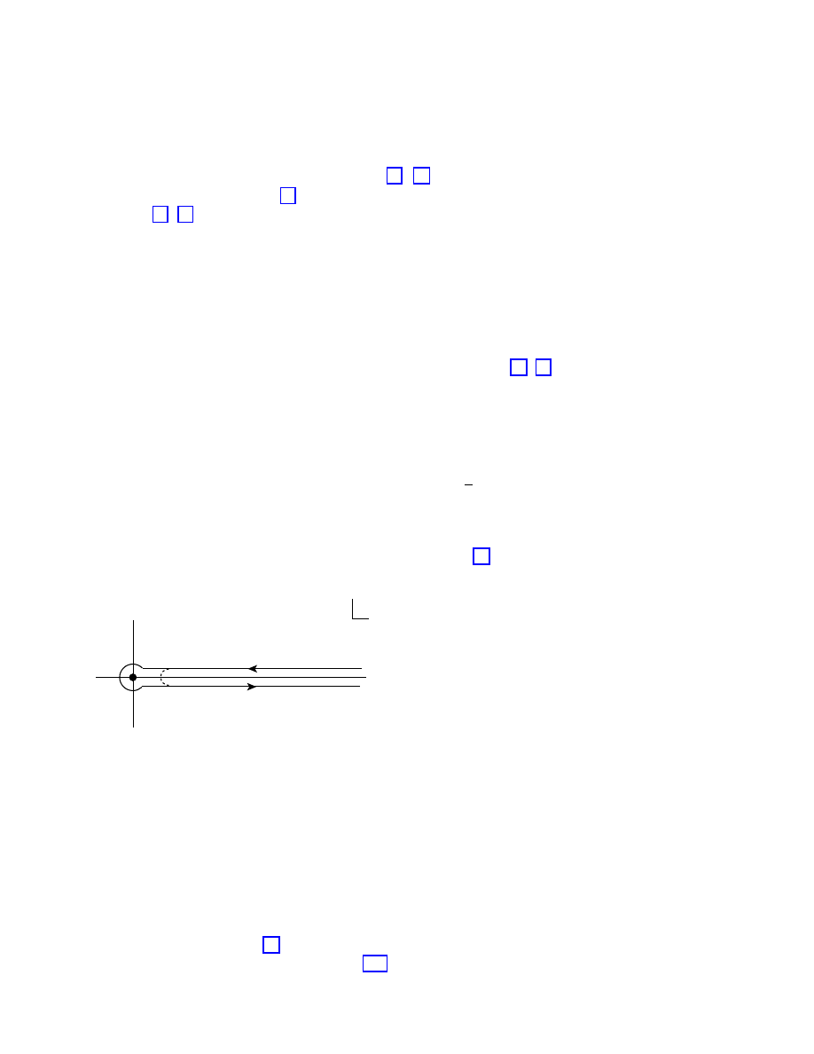
t the Robertson-Walker time, discussed previously in the Lectures. Such vacuum energies
are compatible with recent observations [15, 16], and in fact there is a similarity here
with quintessence models [17], where the rˆole of the quintessence field is played by the
dilaton [23, 25].
4.5
No Scattering Matrix for Liouville Strings
When consider a Liouville string, which as discussed above represents a mathematically
consistent description of a string theory away from its conformal point, the concept of a
string scattering amplitude breaks down. Below, I shall not give a detailed discussion of
this important issue, but I would rather sketch the main reason behind it in a simple way.
For details the interested reader is referred to the literature [23, 20].
Consider a generic correlation function among n vertex operators V
i
of a Liouville
string. In a critical string theory, this can be associated with appropriate on-shell scattering
amplitudes. In Liouville strings, though, with the target-time identified as the Liouville
(RG) mode, this association cannot be made. Let us see briefly why. In such a case the
correlator reads:
hV
i
1
. . . V
i
n
i
g
=
Z
DρDXe
−S
∗
−g
i
R
Σ
d
2
σV
i
+Q
2
∂ρ∂ρ
−Q
2
ρ
R
Σ
d
2
σρR
(2)
V
i
1
. . . V
i
n
(174)
where ρ is the Liouville mode, and Q
2
denotes the central charge deficit, quantifying the
departure of the non-conformal theory from criticality [21].
IR
IR
UV
A
Figure 10: Contour of integration for a proper definition of Liouville field path integra-
tion. The quantity A denotes the (complex) world-sheet area, which is identified with the
logarithm of the Liouville (world-sheet) zero mode. This is known in the literature as the
Saalschutz contour, and has been used in conventional quantum field theory to relate di-
mensional regularization to the Bogoliubov-Parasiuk-Hepp-Zimmermann renormalization
method. Upon the interpetation of the Liouville field as target time, this curve resembles
closed-time-paths in non-equilibrium field theories.
A detailed analysis [23] shows that, upon performing the world-sheet zero-mode ρ
0
integration of the Liouville mode ρ in (174), one obtains that the dominant contributions
55
to the path integral can be represented by a steepest-descent contour of ρ
0
as indicated in
fig. 10. The interpretation of the Liouville zero mode as the target time implies a direct
analogy of this contour with closed time like paths in non-equilibrium field theories [26].
When consider infinitesimal Weyl shifts of the world-sheet metric of the correlators
(174), δ
w
hV
i
1
. . . V
i
n
i, then a straightforward but rather tedious world-sheet analysis shows
that [23]:
δ
w
hV
i
1
. . . V
i
n
i ∝ O
s
A
hV
i
1
. . . V
i
n
i + A − independent terms
(175)
where s =
P
i
α
i
/Q is the sum of the corresponding Liouville anomalous dimensions of the
vertex operators V
i
[21], and Q
2
is the corresponding central charge deficit. The α
i
are
defined such that, if V
i
is not a conformal (marginal) operator, then the “Liouville-dressed”
operator V
L
i
≡ e
α
i
ρ(σ,τ )
V
i
is a marginal operator.
In the scenario of [23], the identification of the world-sheet area (covariant scale) A
with e
−t
, where t is the target time, implies therefore, on account of (175), that these
correlators do exhibit time-dependence, and as such cannot be associated with on-shell
S-matrix elements. Such an association can only be made at the infrared fixed point of
the world-sheet flow, A
→ ∞, where the string reaches its equilibrium position. It should
be mentioned though that the definition of the correlators (174) on the closed-time-like
contour of fig 10 implies that they represent /S elements, associated with density matrices.
To understand better this last point, it suffices to mention that the world sheet partition
function Z of a conformal σ-model, resummed (in general) over world-sheet topologies, is
related to the wavefunctional Ψ[g] of the underlying string theory:
Z[~g]
≡ e
−I
eff
[~
g]
←→ Ψ[~g]
(176)
where I
eff
[~g] =
R
dtd ~
X
L[~g], with t the time, and ~
X spatial coordinates, is the target-space
effective action of the backgrounds ~g, which is the appropriate Legendre transform of the
generating functional of connected correlators in target space.
In the non-critical string approach of [23], discussed here, the time t is nothing other
but the world-sheet zero mode of the Liouville field ρ(σ, τ ). As we have discussed above,
the proper definition of Liouville correlators necessitates an integration of this time variable
over the closed-time-like path of fig. 10. Due to the different sense of the two branches
of this contour, it is then straightforward to see that, upon analytic continuation to the
target-space Minkowski formalism, the middle side of (176) becomes “almost” the product
of ΨΨ
†
(with Ψ(Ψ
†
) associated with, say, the lower (upper) branch of the curve of fig.
10). We say “almost”, because, as discussed in some detail in [23], there are world-sheet
infinities around the turning (ultraviolet) point of the curve (A
∼ 0), whose regularization
(dashed curve in fig. 10) prevents such a complete factorisation. In this sense, the world-
sheet Liouville correlation functions are associated with /S-matrix elements, linking density-
matrices instead of pure quantum states.
In this respect, one might conjecture [20] that an eternally accelerating Universe can
be represented by a (non-equilibrium) Liouville rather than critical string, with the target
time variable being identified with the world-sheet zero mode of the Liouville field. This is
56
consistent with the previous discussion in the beginning of this section, on the impossibility
of constructing a proper S-matrix in such situation, but rather a /S matrix, non factorizable
in SS
†
.
4.6
Graceful Exit from Inflation in Liouville Strings
In the previous section we have argued on the equivalence of a Liouville string theory
with a non-equilibrium dynamical system, for which asymptotic states cannot be defined
properly. From a physical point of view, one of the most interesting applications are the
eternally accelerating Universes, characterized by cosmic (global) horizons beyond which
an observer cannot “see”, and hence the system is open.
Another intereting possibility, however, can arise in the context of non-critical strings,
namely that of a graceful exit from the de Sitter or in general the accelerating phase.
Such a possibility has been discussed in detail in [25], in the context of a specific cos-
mological model based on the so-called type 0-string theory [27]. Such models involve
three-dimensional branes worlds (appropriate stringy domain walls), playing the rˆole of
our observable Universe. We shall not discuss details here, but outline the main results of
that work. Due to the specific choice of a background flux field characterizing the type 0
strings [27], the internal dimensions freeze out after inflation in different sizes in such a way
that one dimension (along the chosen flux background) freezes out to a much larger size
than the others, thereby implying an effectively five-dimensional model. In such a model
the departure from criticality is provided by quantum fluctuations of the three-dimensional
brane worlds.
The model has an inflationary (de Sitter type) phase, characterized by a positive dilaton
potential, and then a smooth exit from it. It is crucial, for consistency of the theory that
the central charge deficit, quantifying the departure from criticality, depends on time.
Immediately after the inflationary period the Universe enters a decelerating phase, which
is succeeded by an accelerating one [25]. The important feature of this model is that,
asymptotically, for large times, it tends to a non-accelerating conformal field theory with a
linear dilaton in the σ-model frame [9] (or, equivalently logarithmic dilaton in the Einstein
frame, depicted in fig. 11). Asymptotically, the dilaton potential, which plays the rˆole of
an (equilibrium) vacuum energy, relaxes to zero as a quintessence like field (173), the rˆole
of the quintessence field being provided by the dilaton. However, we stress again, here
one encounters a non-eternally accelerating quintesssence model. During such phases the
behaviour of the central charge Q
2
(t) is as indicated in figure 11 in the Einstein frame.
Notably, due to the Minkowski signature of the target time (“non-unitary” σ-model field)
there is some oscillation of the central charge before relaxing into its asymptotic infrared
fixed-point value. There is a conformal metastable point at which momentarily the theory
becomes critical (Q
2
= 0), and after this there is some oscillatory behaviour until the
theory settles in its final infrared fixed point. The existence of the conformal metastable
point is a result of the fact that the theory asymptotes to that of a linear dilaton. In such
a case the dilaton equation forces Q to change sign at a certain stage of the evolution [25].
Despite the oscillatory behavior, however, there is an overall decrease of the central charge
57
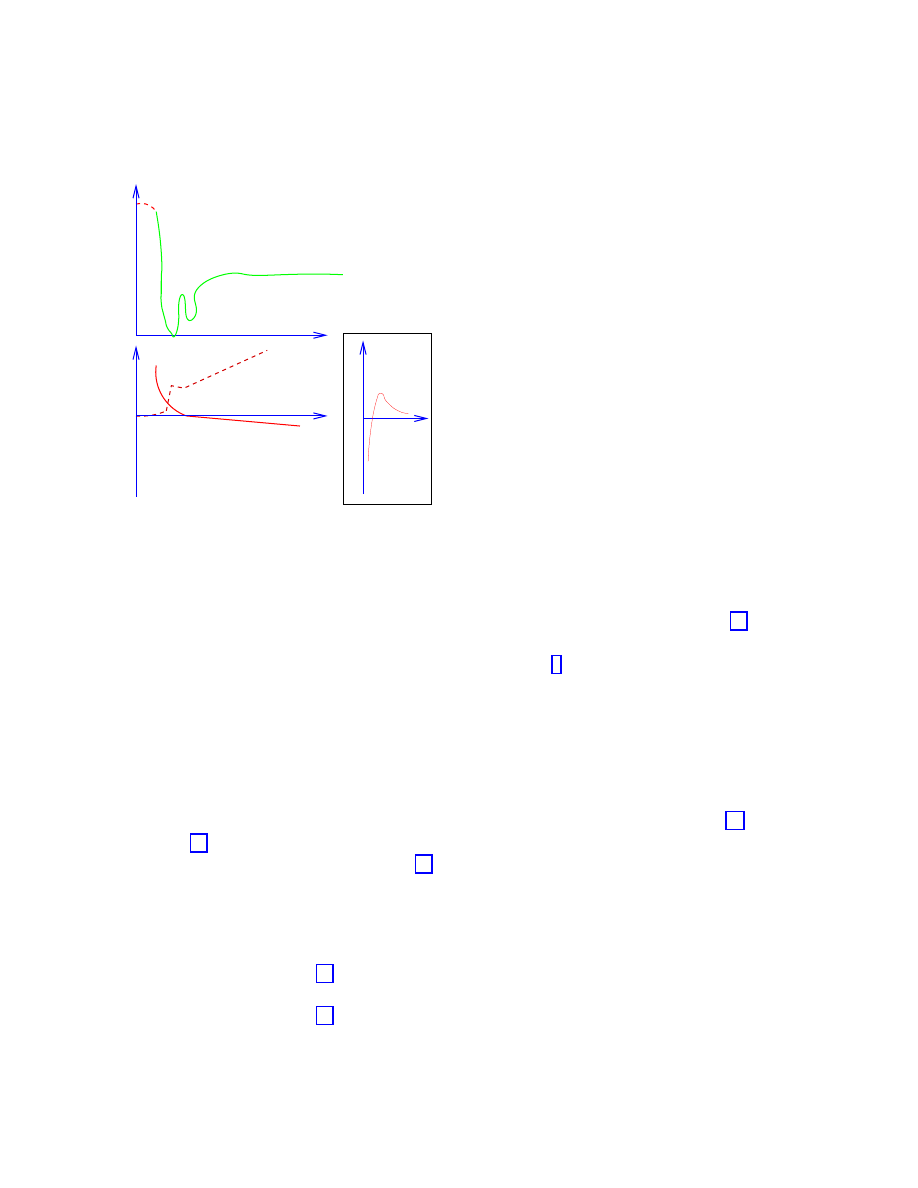
Q
2
0
time
IR fixed point
UV fixed point (?)
Φ
0
time
a,
Φ
Φ
..
a
time
0
a
Figure 11: The behaviour of the central charge deficit (upper) and the dilaton (continuous
line) and scale factor (dashed line) (lower), in the Einstein frame, during the various
evolutionary phases of the cosmological non-critical type-0 string theory of ref. [25]. The
central charge relaxes asymptotically to a constant value, when the model asymptotes, for
large times, to a conformal field theory of the type of ref. [9], describing a non-accelerating
Universe with a negative (logarithmically divergent) dilaton. The diagram inside the box
on the right shows the cosmic acceleration for late Einstein times, indicating the passage
from a decelarating phase after inflation, to an accelerating one, with asymptotic exit from
it.
as it flows from the Gaussian (UV) fixed point value (Big-Bang? Early Universe) to the
infrared one (far future). Unfortunately, the perturbative
O(α
0
) calculations of [25] (solid
line in fig. 11) cannot give sufficient information on the value of the UV fixed point (dashed
line) at present, but we conjectured in [25] that the initial fixed point (constant) value of
Q
2
is also finite, corresponding to a given conformal field theory.
It is interesting to remark that in this model, at late stages of the evolution, the string
coupling g
s
= e
Φ
1, and thus perturbation theory applies. This is due to the fact that
the dilaton asymptotes to
−∞ for large times. This situation has to be contrasted with
the pre-Big-Bang scenario [11] where the weak field regime occurs for early (pre-Big-Bang)
Universes.
The
O(α
0
) analysis of [25] implies initial singularities (Big-Bang type), but, as men-
tioned already, this may be an artifact of the lowest-order truncation. Summing up higher
orders of α
0
corrections, as well as world-sheet topologies, in other words going to a fully
non perturbative string level, may indeed lead to the removal of such singularities. For
58
instance, this is known to be the case in some stringy cosmological models with curvature-
squared corrections of
O(α
02
), in the string effective action [28]. The latter effects are
known to be induced by string loops.
The asymptotic exit from the accelerating phase, and the absence of cosmic horizons
in the model of [25] is a very welcome feature from the point of view of the possibility
of defining asymptotic states [19, 20], and hence a proper S-matrix (for this, however, a
resolution of the initial singularities will be desirable, if not essential). In this respect, our
work is somewhat similar in spirit to the arguments of [29], where eternal quintessence was
argued not to occur in perturbative string theory, which thus was conjectured to exhibit
exit from de Sitter phase, and have a proper S-matrix, calculated though by purely non
perturbative methods.
The basic argument of [29], which however, we stress, should not be considered as a
rigorous proof, can be summarized as follows: in perturbative string cosmology, like the
case examined in [9, 25], but not in PBB scenaria [11] (see fig. 6), the dilaton potential
V
dil
vanishes asymptotically in time, together with the energy E of the dilaton field Φ,
which, in this context, plays the rˆole of a quintessence field. In the framework of (low-
energy) perturbative string-inspired Friedmann-Robertson-Walker Cosmologies, invovling
the (minimal) coupling of the dilaton field to gravity, it can be shown that the existence of
cosmic horizons (147) depends on how fast V
dil
approaches zero as compared with E. In
critical strings, as we have discussed in Lecture 2, a non trivial dilaton potential is generated
through string loops via the Fischler-Susskind mechanism [10] (dilaton tadpoles), and as
such it is given by infinite sums of the form (137), being proportional to various powers of
the string coupling g
s
∼ e
Φ
. In the case of a non-perturbative string potential, then, one
expects such resummations to exponentiate, and in this case V
dil
would be the exponential
function of an exponential of the dilaton field Φ. On the other hand, general arguments [29]
can be given in support of the fact that in perturbative string theory, i.e. in regimes where
the string coupling is weak, so that σ-model perturbation theory is valid, E has at most
a power-law dependence on g
s
. Thus, as Φ
→ −∞, one has that E V
dil
and, therefore,
there will be no cosmic horizon, in the sense that the integral (147) would diverge in the
limit t
→ ∞.
Notice, however, one important difference of the non-critical string approach of [25] from
that of [29]. As just mentioned, in standard critical string theory, a positive cosmological
constant in the effective action, as required by the de Sitter phase, is obtained through
string loops. In contrast, as we have discussed in this Lecture, the non-criticality of the
stringy model of [25] introduces a vacuum energy (dilaton potential) already at a tree
σ-model level.
There are many open issues that are left undiscussed in the non-critical string approach,
regarding the phase after inflation, such as reheating etc. These are open issues for future
work. I must stress though that, although the non-critical string approach to cosmology
appears promising, and already gave physically interesting results, such as the possibility
of graceful exit from de Sitter (and in general accelerating) Universe phase, nevertheless
it is still very far from being considered as well established. So far we have treated the
departure from criticality at a “phenomenological” level, by treating the time dependence of
59
the central charge deficit as being determined by consistency with the rest of the Liouville
conditions (168), which replace the conformal invariance (64) conditions of the critical
strings. To be complete one should discuss explicitly the internal conformal field theory
(pertaining to the extra dimensions), whose ‘flow’ between fixed points results in the Q(t)
under consideration. Moreover, from the physical viewpoint one should also examine the
rˆole of supersymmetric target-spaces in cosmological scenaria. Note that even in the case of
type-0 strings, with explicitly broken supersymmetry, fermionic target-space backgrounds
do exist, given that the original underlying theory is a superstring [27]. These issues present
important theoretical challenges, awaiting further studies, which, in my personal opinion,
is something that should be done.
5
Conclusions
In these lectures I have tried to give a brief account of interesting cosmological scenaria
from the point of view of string theory. As we have seen, there are amusing possibilities,
such as a pre-Big-Bang life of the Universe, graceful exit from accelerating Universe phases
etc., which do not seem to be characterizing conventional cosmological models.
Recent experimental developments in the field of astrophysics, concerning for instance
the possibility for the current era of the Universe to be an accelerating phase, present
important theoretical challenges for string theory, which probably necessitate a fresher
look at string cosmology. One such possibility might be the representation of a cosmo-
logical (time-dependent) background of string theory as a non-critical (non-conformal),
non-equilibrium situation. Although speculative, such a possibility seems, at least to the
me, a mathematically viable one, if the non-conformal nature of the background is seen
from the point of view of a renormalization-group flow between fixed (equilibrium) points
in string theory space.
In this context it should be mentioned that there are many explicit models one can
construct, which exhibit graceful exit from de Sitter, or, in general, accelerating phases.
One of them was presented in [25], and analysed briefly in these lectures. Additional non-
critical string models with such exit properties can be found in toy two-dimensional non-
critical stringy cosmologies [30], where the non-criticality is induced by initial fluctuations
of matter backgrounds. Moreover, in higher-dimensional theories, one encounters such
graceful exit properties in cases of intersecting brane cosmologies. For instance, it can be
shown that if one represents our universe as a three-brane domain wall, punctured with D-
particles (point-like solitonic defects) [31], then recoil of these D-particle during scattering
with macroscopic numbers of closed string states propagating on the brane can also lead
to space-time back reaction, which is sufficient to induce exit from an accelerating phase,
so that the final equilibrium theory will again asymptote to a conformal field theory of the
type of ref. [9].
In general, there are many issues in the context of string cosmology that remain open,
apart from the exit problem. Issues like reheating after the inflationary phase, the rˆole
of supersymmetry in inflationary scenaria etc, are some of them. We have not touched
60

such issues here, but we believe that we have presented enough material in this admitedly
brief and by far not complete exposition, which would motivate the interested reader to do
further research in the exciting directions opened up by string cosmology.
Acknowledgements
I would like to thank the organizers of the First Aegean School on Cosmology for creating
an excellently organized, very successful and thought stimulating school, in a very pleasant
and relaxed atmosphere.
References
[1] M.B. Green, J.H. Schwarz, E. Witten: Superstring Theory, Vols I and II (Cambridge
University Press, Cambridge 1987).
[2] J. Polchinski, Phys. Rev. Lett. 75, 4724 (1995); TASI lectures on D-branes, hep-
th/9611050; M. J. Duff, Sci. Am. 278, 64 (1998).
[3] A.B. Zamolodchikov, JETP Lett. 43, 730 (1986).
[4] N.E. Mavromatos, J.L. Miramontes, J.M. Sanchez de Santos: Phys. Rev. D 40, 535
(1990).
[5] I. Klebanov, L. Sussking: Phys. Lett. B 200, 446 (1988).
[6] H. Osborn: Phys. Lett. B 214, 555 (1988); Nucl. Phys. B 363, 486 (1991).
[7] G. Curci, G. Paffuti: Nucl. Phys. B 286, 399 (1987).
[8] P. Kanti, N. E. Mavromatos, J. Rizos, K. Tamvakis, E. Winstanley: Phys. Rev. D
54, 5049 (1996); S. O. Alexeev, M. V. Pomazanov: Phys. Rev. D 55, 2110 (1997).
[9] I. Antoniadis, C. Bachas, J. R. Ellis, D. V. Nanopoulos: Phys. Lett. B 211, 393
(1988); Nucl. Phys. B 328, 117 (1989); Phys. Lett. B 257, 278 (1991).
[10] W. Fischler, L. Susskind: Phys. Lett. B 171, 383 (1986);ibid. B 173, 262 (1986).
[11] G. Veneziano, in Les Houches 1999, The primordial universe, p. 581-628 (North
Holland 1999) [hep-th/0002094], and references therein.
[12] M. Gasperini, J. Maharana, G. Veneziano: Phys. Lett. B 296, 51 (1992).
[13] K. .A. Meissner, G. Veneziano: Mod. Phys. Lett. A 6, 3397 (1991);
61
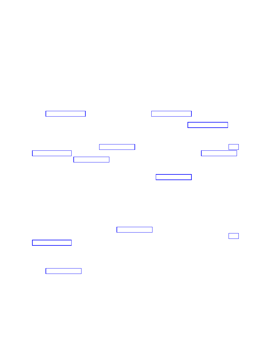
[14] M. Gasperini, J. Maharana, G. Veneziano:
Nucl. Phys. B 472, 349 (1996);
M. Gasperini, G. Veneziano: Ge. Rel. Grav. 28, 1301 (1996); A.A. Kehagias,
A. Lukas: Nucl. Phys. B 477, 549 (1996); A. Buonanno, M. Gasperini, M. Mag-
giore and C. Ungarelli, Class. Quant. Grav. 14, L97 (1997).
[15] S. Perlmutter et al. [Supernova Cosmology Project Collaboration]: Nature 391, 51
(1998); A. G. Riess et al. [Supernova Search Team Collaboration]: Astron. J. 116,
1009 (1998); P. M. Garnavich et al., Astrophys. J. 509, 74 (1998).
[16] J.R. Bond, A.H. Jaffe and L. Knox, Phys. Rev. D 57, 2117 (1998); H. Lineweaver,
astro-ph/9810334; N. A. Bahcall and X. Fan, astro-ph/9804082.
[17] For a review see: S. M. Carroll, Living Rev. Rel. 4, 1 (2001) [astro-ph/0004075].
[18] S. W. Hawking, Commun. Math. Phys. 87, 395 (1982).
[19] T. Banks, W. Fischler: hep-th/0102077; S. Hellerman, N. Kaloper, L. Susskind: hep-
th/0104180; W. Fischler, A. Kashani-Poor, R. McNees, S. Paban: hep-th/0104181;
E. Witten, hep-th/0106109; P. O. Mazur, E. Mottola: Phys. Rev. D 64, 104022
(2001), and references therein.
[20] J. Ellis, N. E. Mavromatos, D. V. Nanopoulos: hep-th/0105206.
[21] F. David, Modern Physics Letters A3, 1651 (1988); J. Distler, H. Kawai: Nucl.
Phys. B321, 509 (1989).
[22] C. Schmidhuber, A. A. Tseytlin: Nucl. Phys. B 426, 187 (1994).
[23] J. Ellis, N. E. Mavromatos, D. V. Nanopoulos: Phys. Lett. B293, 37, (1992);
Mod. Phys. Lett. A10 (1995) 1685; for reviews see: Erice Subnuclear Series (World
Sci., Singapore) 31 1, (1993); [hep-th/9304133]; J. Chaos, Solitons and Fractals 10,
345 (eds. C. Castro amd M.S. El Naschie, Elsevier Science, Pergamon 1999) [hep-
th/9805120], and references therein.
[24] D. Kutasov, N. Seiberg: Nucl. Phys. B 358, 600 (1991).
[25] G. A. Diamandis, B. C. Georgalas, N. E. Mavromatos, E. Papantonopoulos, I. Pappa:
[26] The CTP formalism may be attributed to: J. Schwinger, J. Math. Phys. 2, 407
(1961); for reviews see: E. Calzetta and B.L. Hu, Phys. Rev. D37, 2878 (1988); E.
Calzetta, S. Habib and B.L. Hu, Phys. Rev. D37, 2901 (1988); H. Umezawa, Ad-
vanced Field Theory: micro, macro and thermal concepts (American Inst. of Physics,
N.Y. 1993).
[27] I. Klebanov, A.A. Tseytlin: Nucl. Phys. B546, 155 (1999); Nucl. Phys. B547, 143
(1999).
62

[28] See, for instance: I. Antoniadis, J. Rizos and K. Tamvakis, Nucl. Phys. B 415, 497
(1994).
[29] T. Banks and M. Dine, JHEP 0110, 012 (2001) [hep-th/0106276].
[30] G. A. Diamandis, B. C. Georgalas, N. E. Mavromatos, E. Papantonopoulos: Phys.
Lett. B461, 57 (1999).
[31] E. Gravanis, N. E. Mavromatos: hep-th/0106146.
63
Wyszukiwarka
Podobne podstrony:
Black Holes & Gravitational Waves in String Cosmology(1998)
IIA Statistical Physics and Cosmology 2
Physics Papers Edward Witten (2000), The Cosmological Constant From The Viewpoint Of String Theory
Physics Papers Steven Weinberg (2003), Damping Of Tensor Modes In Cosmology
Physics Papers Lee Smolin (1993), Time, Measurement And Information Loss In Quantum Cosmology
Cosmology for String Theorist
Physical Interpretation of the 26 Dimensions of Bosonic String Theory
Physics Papers Andrei Linde (2003), Testing The Cosmological Constant As A Candidate For Dark Energ
KOLE The arrow of time in cosmology and statistical physics (termodynamics, reductionism)
The Quantum Physics of Black Holes and String Theory
hawking the future of quantum cosmology
ligeti string quartet nr 2 (fragment) 37TIJMK7OLN55XATRZELIHMKA7GXBO6SJAWMOOA
Basic Radiation Physics
Current Clinical Strategies, Physicians' Drug Resource (2005) BM OCR 7 0 2 5
HE Solo Strings Giga3 artfiles
DSaA W13 String Matching
Feynman Lectures on Physics Volume 1 Chapter 04
więcej podobnych podstron