Taxonomy and Effectiveness of Worm Defense Strategies

Taxonomy and Effectiveness of Worm Defense

Strategies

David Brumley, Li-Hao Liu, Pongsin Poosankam, and Dawn Song

June 2005

CMU-CS-05-156

School of Computer Science

Carnegie Mellon University

Pittsburgh, PA 15213

Abstract

While it is important to develop effective worm defense techniques, most previous work has focused on a

single point in the design space. The sheer complexity and size of the design space of worm defense requires

a more systematic study of the design space.

We give the first systematic investigation of the design space of worm defense system strategies. We ac-

complish this by providing a taxonomy of defense strategies by abstracting away implementation-dependent

and approach-specific details and concentrating on the fundamental properties of each defense category. Our

taxonomy and analysis reveals the key parameters for each strategy that determine its effectiveness. We pro-

vide a theoretical foundation for understanding how these parameters interact, as well as simulation-based

analysis of how these strategies compare as worm defense systems. Finally, we offer recommendations based

upon our taxonomy and analysis on which worm defense strategies are most likely to succeed. In particular,

we show that a hybrid approach combining Proactive Protection and Reactive Antibody Defense is the most

promising approach and can be effective even against the fastest worms such as hitlist worms. Thus, we are

the first to demonstrate that it is possible to defend against the fastest worms such as hitlist worms.

Keywords:

worms, worm propagation, defense strategy analysis, proactive protection, probabilistic

protection, address space randomization, worm blacklisting, worm antibody, worm containment, automatic

worm containment

Introduction

Internet worms can cause millions of dollars of damage by infecting hundreds of thousands of hosts in a

short period of time [25, 16]. As a result, considerable research effort has been spent developing worm

defense systems [12, 13, 17, 19, 20, 22, 23]. While most previous work focuses on a single isolated point

in the design space of worm defenses, the sheer complexity and size of the design space of worm defense

requires a more systematic and global-view approach. A global-view approach assists us in understanding

the fundamentals of worm defense, identifying new directions and points in the design space, and developing

more effective defense strategies.

Despite the importance, little research has been done in systematically analyzing the design space of

worm defense systems. Previous work by Moore et al. [14] and Porras et al. [20] has systematically analyzed

more than one point in the design space. Their studies were limited in scope because they analyzed only a

few combinations of proposed worm defense techniques. A general and systematic framework that explores

the entire worm defense landscape has been an open problem.

In this paper, we provide the first systematic study of the complete worm defense design space. We

provide the first taxonomy of worm defense system strategies. Our taxonomy provides an abstract frame-

work and categorizes worm defense strategies based upon fundamental implementation-independent and

approach-generic factors. This abstract framework enables us to pinpoint the key factors of each defense

category that determines its effectiveness.

We conduct theoretical modeling and analysis as well as simulation evaluations of the effectiveness of

each defense category against various worms, including random scanning and hit-list worms. Our analysis

reveals the fundamental strengths and weaknesses of each defense category which provide important insight

in designing new systems.

Our analysis yields fresh observations that provide new view points to previous beliefs. For example,

previous work investigated the limitations of diversity in hosts as a protection measure [21]. Our taxonomy

and analysis gives insight into how diversity – an example of our Proactive Protection category – is an

important and practical worm defense strategy in many circumstances. In particular, Proactive Protection is

extremely important in defending against super-fast worms such as hit-list scanning worms [25] (Section 5

& 6.2).

As another example, rate limiting – an example of our Local Containment category – is an often proposed

worm defense solution [26]. From our analysis, we are able to show that any Local Containment strategy is

fundamentally limited in any realistic scenario where it is only partially deployed. For example, if 1/2 of the

internet deployed such a strategy, current worms are slowed down by only a factor of 2. Other strategies are

likely more practical since they achieve a larger slowdown with a smaller fraction of deployment (Section 5).

Note that in this paper we focus on worm defense mechanisms that reduce the number or the speed at

which hosts are infected. Other mechanisms that assist in recovery or cleanup after-the-fact are orthogonal

to our goal, and could be used in conjunction with any defense mechanism to reduce the total cost of a worm

infection.

Contributions.

In this paper, we make the following contributions:

•

We provide the first taxonomy of worm defense strategies. This taxonomy allows us to systematically

analyze the design space of worm defense, and is useful for abstracting away approach-specific details

and investigating the fundamental strengths and weaknesses of the different strategies. Our taxonomy

shows each strategy has unique key factors that determine its effectiveness besides the standard false

positive and false negative analysis.

•

We propose a list of evaluation criteria to guide our analysis and evaluation of each defense category.

We then conduct theoretical analysis of the effectiveness of each defense strategy in our taxonomy.

To confirm our theoretical analysis, we conduct simulation evaluations for each strategy category with

two real worms (Slammer and CodeRed) as well as theoretical hit-list worms which are among the

fastest worms [25]. Our simulation evaluation confirms our theoretical analysis. Our analysis provides

the first comparison between overall worm defense strategies.

•

We use our results to craft recommendations for which strategies show the most promise. We show that

a combination of Proactive Protection and Reactive Antibody Defense is the most effective defense

and shows promise even against the fastest worms such as hit-list worms.

•

As part of our analysis of the fundamental limits of the defense strategies, we design and investigate

a new class of worms, called brute-force worms, that specifically target the weakness of Proactive

Protection strategies. We design defense systems capable of defending against brute-force worms

(Section 6.1).

Organization

We begin by considering the entire worm defense design space, which we divide into a

taxonomy of related strategies (Section 2). We then provide a theoretical framework for each defense strategy

in the taxonomy for both when employed alone and in combination (Section 3 & 4).

Next, to confirm our theoretical analysis, we perform simulation evaluation for the effectiveness of each

category for real-world worms, CodeRed and Slammer, (Section 5), as well as faster worms such as hit-list

worms (Section 6). We also develop a new smart worm against Proactive Protection defenses. We analyze

the effectiveness of this worm, along with potential defenses (Section 6.1).

Finally, we use the result of our theoretic and simulation modeling to provide recommendations for new

worm defense systems (Section 8). The recommendations show that a hybrid approach combining Proactive

Protection and Reactive Antibody Defense is the best approach to stop tomorrow’s smart worms.

Defense Strategies

In this section, we first propose a taxonomy of worm defense strategies. We then propose the evaluation

criteria for worm defense strategies. The following sections make use of the taxonomy and evaluation criteria

to analyze and compare the different strategy categories.

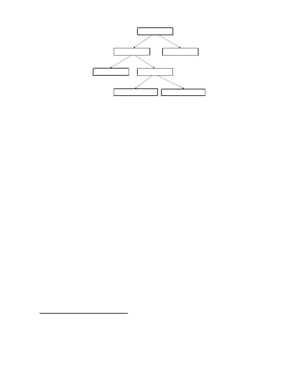
2.1

Defense Strategy Taxonomy

To systematically analyze the design space of worm defense strategies, we first observe that in order to

defend against worm attacks, we can take two fundamentally different approaches: either protect vulnerable

machines from incoming worm attacks, or contain a local infection from sending outgoing attacks to spread

the worm (which we call Local Containment). Note that most proposed systems fall into the former category

which we further divide into proactive defense which is not dependent on any specific worm (which we call

Proactive Protection) and reactive defense which needs specific information about the worm outbreak to be

effective. We then further divide the reactive defense into two subcategories based on whether the defense

uses the information about the content of the traffic (which we call Reactive Antibody Defense) or the sender

of the traffic (which we call Reactive Address Blacklisting) (Figure 1). We describe the four categories

below:

Strategy 1: Reactive Antibody Defense.

In immunology, an antibody is a protein generated in reaction to

and acts against a specific antigen. Similarly, a Reactive Antibody Defense strategy automatically generates

an inoculation in response to a worm that when applied will protect hosts from infection. An example of

Defense Strategies

Protection

Local Containment

Proactive Protection

Reactive Protection

Reactive Address Blacklisting

Reactive Antibody Defense

Figure 1: Worm Defense Strategy Taxonomy

such an antibody-based strategy is to automatically generate and deploy content-based signatures [12, 13,

14, 17, 19, 23] to filter out worm traffic. System patching is also a type of antibody [22]

Besides the standard false positive rate and false negative rate, a key factor determining the effectiveness

of this strategy is the time it takes to create and disseminate the antibody, which we call the reaction time,

denoted as δ

. Intuitively, the longer it takes to create and disseminate the antibody, the more hosts a worm

can infect.

Strategy 2: Reactive Address Blacklisting.

Instead of generating a worm-specific antibody as a defense,

another approach is to identify the infected machines and filter out packets from them to protect vulnerable

hosts from their attacks. We call the list of host addresses that are infected and who therefore should be

blocked [14] the address blacklist, and this defense strategy Reactive Address Blacklisting.

Reactive Address Blacklisting differs from the Reactive Antibody Defense approach in that Reactive

Address Blacklisting blocks worm infection attempts by recognizing that they are from infected (black-

listed) hosts, where Reactive Antibody Defense blocks worm infection attempts by recognizing that they

are malicious packets irrespective of where they come from. While Reactive Antibody Defense is effective

against a worm attack irrespective of where it comes from, Reactive Address Blacklisting can only be used

to block out attacks from the hosts on the address blacklist (and will not be effective against attacks where

address spoofing is possible such as UDP worm attacks). Thus, unlike Reactive Antibody Defense which

only needs to create the antibody effective against the worm, the Reactive Address Blacklisting approach

needs to identify each infected host as soon as it becomes infected and adds it to the address blacklist.

Similarly to the Reactive Antibody Defense approach, the effectiveness of Reactive Address Blacklisting

is determined by the time for creating and installing the appropriate blacklists, which we call the reaction

time, δ

. Note δ

in Reactive Antibody Defense is the reaction time to create and disseminate an antibody

once the worm has started, while δ

here is the reaction time to put a host on the (global) blacklist after it

becomes infected.

Strategy 3: Proactive Protection.

Instead of generating antibodies or blacklists reacting to a specific

worm or infection attempt, another defense approach is to proactively harden the system to make it difficult

for a worm to exploit vulnerabilities and successfully infect the host on any single attempt. We call this

category of defense Proactive Protection. There are many different methods for proactively hardening a

Similarly, port filtering could be a type of antibody defense, though most implementations suffer from poor accuracy due to the

rough filtering granularity afforded by this method.

We abstract away implementation details by assuming the blacklist is a single global list that is universally updatable.

system, including sandboxing, privilege separation, system call monitoring, etc. For a specific worm attack,

a proactive protection mechanism may be completely effective in which case it will protect the vulnerable

hosts from the attack (although some protection mechanisms work not by preventing a successful exploit of

the vulnerability, but rather by preventing the exploit to do damage to or control the host); or the proactive

protection may be only partially effective in which case it can only protect the host sometimes or in some

cases. One specific example of the latter case is diversity-based approach, which delays infection of a

vulnerable host by increasing the entropy of each individual host such that an internet worm on average

needs multiple trials to compromise the host. For example, most exploits in worm attacks require knowledge

of specific run-time internal states of the vulnerable host. Various address-space randomization techniques

have been proposed to randomize run-time memory layout [1, 4, 5, 6, 8, 9, 28], preventing a worm from

knowing the correct address a priori for a successful exploit. Other techniques such as pointer encryption [7],

instruction set randomization [2, 3, 11, 24], password protection schemes, etc., also fall into this category as

they make the system harder to attack by increasing the entropy of information needed for the attack to be

successful. Note that the analysis in this paper only applies to the case of probabilistic Proactive Protection

such as the diversity-based Proactive Protection.

The amount of entropy directly affects the probability p, called the protection probability , of a single

worm exploit attempt succeeding in infecting a vulnerable host. Worms attacking hosts implementing Proac-

tive Protection must make about 1/p exploit attempts to infect a host. The protection probability is thus the

key factor determining the effectiveness of the Proactive Protection approach.

Note that one salient advantage of Proactive Protection is that it is a proactive defense always in place

unlike a reactive measure. The defense is not based on any specifics of the vulnerability and does not need

any triggered reaction to deploy to the vulnerable hosts. However, the defense only increases the work factor

for a worm to successfully infect, and is not full-proof protection. Hence, eventually a long-term fix must be

applied for permanent protection.

Strategy 4: Local Containment.

A Local Containment strategy focuses on containing a locally infected

machine from sending attack traffic to other potentially vulnerable hosts, e.g., filter based upon outgoing

connections instead of the previous three approaches which focused on incoming connections. Local Con-

tainment strategies thus exemplify a “good neighbor” policy, where more good neighbors result in fewer

worm attacks.

Scan rate throttling schemes such [26, 27] are the primary example of Local Containment. The throttle

rate reduces the contact rate of current infections, thus slowing down the overall worm propagation speed.

The throttling rate is an important factor for containing the worm propagation speed, however, a more

important factor is the deployment rate. As we will show in the next section, the effectiveness of Local

Containment is proportional to the fraction of hosts deploying the defense, and consequently requires a very

high deployment ratio in order to contain a worm outbreak. Even when deployed on 90% of the hosts and

networks, i.e., 90% of the hosts and networks are good neighbors, it will not affect attacks coming from the

other 10% of hosts and networks, and thus can only slow down the worm propagation by a factor of 10.

2.2

Evaluation Criteria

A worm defense strategy can be evaluated in two dimensions: how well it contains a worm outbreak vs. how

many hosts participant in the defense. Let N = N

+ N

be the total number of vulnerable hosts, where N

of the vulnerable hosts participate in the defense system (which we call participating hosts) and N

do not

(which we call non-participating hosts). Let I(t) = I

(t) + I

(t)

be the total number of infected hosts at

time t, where I

(t)

is the number of participating hosts infected and I

(t)

the number of non-participating

hosts infected.

Incremental Deployment.

It is unrealistic to assume any scheme will be immediately and fully deployed

overnight. The deployment ratio α =

is the number of vulnerable hosts participating in the protection

strategy over the total number of vulnerable hosts. All other things being equal, strategies with lower α

values are preferable since they require fewer participants to be effective.

Infection Factor.

This factor measures the fraction of vulnerable hosts being infected at time t, which

measures how well a worm defense system protects hosts from infection, with lower values indicates fewer

hosts infected.

Worm defense strategy effectiveness can therefore be measured in two ways:

•

Overall Infection Factor:

The ratio of the number of hosts that are infected at a given time to the

total number of vulnerable hosts, e.g.,

(t)

. When no hosts are infected the infection factor is 0%,

while when all hosts are infected the infection factor is 100%. This is the most common measure of

effectiveness.

•

Participation Infection Factor and Non-participation Infection Factor:

In a partial deployment

scenario where only some hosts deploy the defense, the hosts and networks that deploy the defense

(which we call participating hosts) may have a different likelihood of becoming infected than those

that do not deploy the defense (which we call non-participating hosts). This difference, in fact, can be

an important incentive to convince more hosts and networks to deploy the defense. To measure this

difference, we propose two new effectiveness measures: the participation infection factor (PIF) as the
ratio of the number of participating-hosts infected to the total number of participating hosts, e.g.,

(t)

;

and the non-participation infection factor (NPIF) as the ratio of non-participating hosts infected to the
total number of non-participating hosts, e.g.,

(t)

If a defense approach incurs no difference in the likelihood of being infected between a participating

host or a non-participating host, then the participation factor and the non-participation factor will

be the same, which gives little incentive for hosts and networks to deploy the defense approach. For

example, as our analysis in the next section shows, Local Containment gives no difference between the

participation infection factor and the non-participation infection factor. On the other hand, a defense

system with positive deployment incentive should give a much lower participation infection factor than

the non-participation infection factor, as the case for Reactive Antibody Defense, Reactive Address

Blacklisting, and Proactive Protection.

Theoretical Analysis of Worm Defense Strategies

In this section, we analyze the effectiveness of the different worm defense strategies in our taxonomy. We

first review worm modeling background, and then give our theoretical analysis of the effectiveness of the

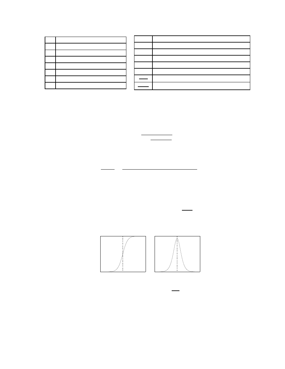
different worm defense strategies. Our notation is summarized in Table 1.

3.1

Worm Modeling Background

Worm propagation can be well described with the classic Susceptible-Infected epidemic model [10]. The

overall rate of new infections is given in this model by:

dI(t)

βI(t)(N − I(t))

(1)

Equation 1 states the rate of new infections is equal to the product of the number of infected hosts, the

average contact rate of each infected host (β), and the fraction of uninfected hosts.

We solve equation 1 for the number of hosts infected at time t (I(t)) with C initially infected hosts as:

Deployment ratio

Vulnerable host contact rate

Throttle rate

Reaction time (Antibody)

Reaction time (Blacklist)

Protection probability

Timestamp

# of initial infected hosts = I(0)

# of all vulnerable hosts

# of participating vulnerable hosts

# of non-participating vulnerable hosts

I(t)

# of hosts infected at time t

(t)

# of participating hosts infected at time t

(t)

# of non-participating hosts infected at time t

(t)

Rate of new infections

(t)

Acceleration of new infections

Table 1: Notation and Parameters Used in Our Analysis

I(t) =

1 +

−βt

(N −C)

(2)

This shows that the worm contact rate β is the important factor for determining its propagation speed.

We can also find the acceleration of a worm, given by:

I(t)

tβ

(C − N )(C + Ce

tβ

−

N )N

(C(e

tβ

−

1) + N )

(3)

When a typical worm is first released, it will first undergo an acceleration phase because vulnerable hosts

are easy to find. At some point the worm will slow down either because there are few uninfected vulnerable

hosts left or the defense scheme makes them harder to infect. We call the point at which a worm begins to

slow down the breaking point t

. As shown in Figure 2, t

is useful because it divides a worm’s lifetime into

two phases: acceleration and deceleration, and can be calculated as

(t)

= 0

. The t

reference point is

useful for many categories because it indicates whether the defense slows down a worm prior to its natural

breaking point.

→

Worm Speeding Up

←

→

Worm Slowing Down

←

Time

Infected Machines (I(t))

(a) Number of infections

over time I(t)

→

Worm Speeding Up

←

→

Worm Slowing Down

←

Time

Rate of New Infected Machines ( dI(t)/dt)

(b) Rate of new infections

over time

(t)

Figure 2: (a) shows infections as a function of time. (b) shows the rate of new infections. As shown, t

divides the lifetime of a worm into two phases: acceleration and deceleration.

3.2

Effectiveness of Proactive Protection

We first analyze the effectiveness of Proactive Protection with full deployment (I(t) = I

(t)

). We can

derive the time evolution of the number of infected hosts I(t) with an average contact rate β and protection

probability p as below:

dI(t)

pβI(t)(N − I(t))

(4)

The solution to Equation 4 with C initially infected hosts is:

I(t) =

1 +

−pβt

(N −C)
C

(5)

The above analysis shows that Proactive Protection slows down the worm propagation by a factor of 1/p.

We now consider partial deployment (I(t) = I

(t) + I

(t)

) where α fraction of the vulnerable hosts

deploy Proactive Protection. We derive the time evolution of the number of infected hosts participating

(t)

) and not participating (I

(t)

) as:

(t)

βαpI(t)(N

−

(t))

(6)

(t)

β(1 − α)I(t)(N

−

(t))

(7)

Equation 6 shows the worm infection rate for the α protected hosts is reduced by less than

1
p

since

non-participating infected hosts also contribute to protected host infections.

Since Proactive Protection is a proactive defense, one may wish to calculate the protection probability

needed to ensure a given breaking point t

. We calculate this as follows:

1 +

−pβt

(N −C)

= 0

(8)

By solving Equation 8 for p, we get:

p =

N −C

βt

(9)

3.3

Effectiveness of Reactive Antibody Defense

We first analyze the effectiveness of Reactive Antibody Defense techniques with full deployment (I(t) =
I

(t)

). Assuming the reaction time for generating and disseminating the (perfect) antibody is δ

, we derive

the time evolution of I(t) as:

dI(t)







βI

(t)(N −I(t))

when t ≤ δ

when t > δ

(10)

Equation 10 mirrors the idea that before an antibody is found all hosts are completely unprotected (t ≤

), but after antibody is created and disseminated (t > δ

) no further infections occur. Therefore, antibody

strategies should minimize δ

The solution to Equations 10 with C initially infected hosts is:

I(t) =











e−βt

(N −C)

when t ≤ δ

e−βδa

(N −C)

when t > δ

(11)

Now we consider partial deployment (I(t) = I

(t) + I

(t)

) when α fraction of the vulnerable hosts are

protected by Reactive Antibody Defense.

(t)











βαI

(t)(N

−I

(t))

when t ≤ δ

when t > δ

(12)

(t)

β(1 − α)I(t)(N

−

(t))

(13)

The solution to the system of differential equations is:

I(t) =

1 +

−βt

(N −C)

when t ≤ δ

(14)

(t) = I

(δ

)

when t > δ

(15)

(t) =

(δ

−

1 + A

−

1 + A

−

(δ

)

when t > δ

(16)

where

A = e

tβIp(δa)

Nnp

+tβ−

tβαIp(δa)

Nnp

−tβα−

A2Ip(δa)

NnpA1

−

A2αIp(δa)

NnpA1

A2α

= −I

(δ

) − N

+ αI

(δ

) + αN

= −δ

βI

(δ

) − δ

βN

+ δ

αI

(δ

) + δ

αN

+ N

ln (−

(δ

) + I

(δ

)

−

(δ

)

The above analysis shows that given the reaction time δ

, the deployment ratio has no influence on the

protection of participating hosts. Non-participating hosts indirectly benefit from a larger deployment ratio

after t > δ

. The reason is at this point uninfected participating hosts are effectively removed from the

vulnerable population, resulting in a slower worm propagation.

3.4

Effectiveness of Reactive Address Blacklisting

We first analyze Reactive Address Blacklisting techniques with full deployment (I(t) = I

(t)

). The reaction

time δ

is the time to add a newly infected host to the global blacklist. We derive the time evolution of the

number of infected hosts I(t) as:

dI(t)

β(I(t) − I(t − δ

))(N − I(t))

(17)

Now we consider the case when the Reactive Address Blacklisting is deployed to cover α fraction of the

vulnerable hosts (I(t) = I

(t) + I

(t)

βα(I(t) − I(t − δ

))(N

−

(t))

(18)

(t)

β(1 − α)I(t)(N

−

(t))

(19)

These equations quantify the intuition that a smaller reaction time slows down a worm’s propagation.

Here, we briefly discuss the minimum reaction time required for an effective defense. Intuitively, if we

can add a newly infected machine to the blacklist before it infects another machine, the Reactive Address

Blacklisting defense may stop the exponential worm growth. Within each time unit the infected nodes can

contact β vulnerable hosts. Thus, if the reaction time δ

is faster than

, then the worm propagation to

the hosts that deploy the defense can be effectively stopped. We call this threshold

the phase transition

threshold

. On the other hand, if the reaction time δ

is slower than

, then the worm propagation cannot be

stopped and will eventually infect all the vulnerable hosts. Thus, the requirement for an effective Reactive

Address Blacklisting is to ensure

≤

(20)

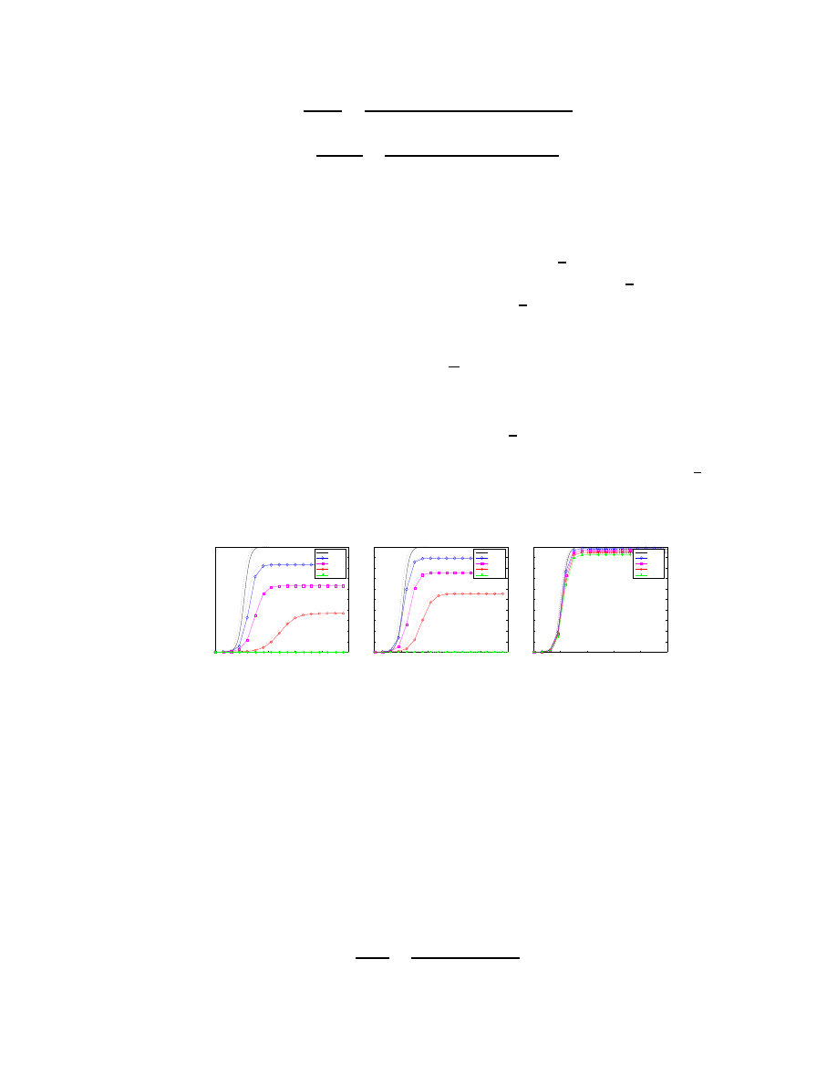
To demonstrate the effect of the phase transition threshold, we depict in Figure 3 the influence of the

reaction time on the effectiveness of Reactive Address Blacklisting, obtained from both theoretical analysis

and simulation results. Note that the phase transition threshold,

, is about 10 seconds for Slammer. The

graphs show that our theoretical analysis (dotted lines) match well our simulation results (solid lines). From

the graphs, we can clearly see that the defense is effective when the reaction time is lower than

. In these

cases, the number of infected machines for 100% deployment is close to zero. On the other hand, if δ

is far

higher, even 100% deployment of Reactive Address Blacklisting cannot stop the spread of worm.

100

200

300

400

500

100

Time ( in seconds)

infected machines (%)

=0.25

=0.5

=0.75

(a) 5 sec.(S.L)

100

200

300

400

500

100

Time ( in seconds)

infected machines (%)

=0.25

=0.5

=0.75

(b) 10 sec.(S.L)

100

200

300

400

500

100

Time ( in seconds)

infected machines (%)

=0.25

=0.5

=0.75

Figure 3: The reaction time for Reactive Address Blacklisting . We compare the effectiveness of the Reactive

Address Blacklisting strategy against Slammer with different reaction times. The experimental data (solid

lines) and the theoretical data (dotted lines) match well. When the reaction is low enough, as in (a) and (b),

the number of infected machines for 100% deployment is very close to zero.

3.5

Effectiveness of Local Containment

We consider the case where α fraction of vulnerable hosts are covered by a Local Containment mechanism.

The full deployment case is easily derived with α = 1. Assume the throttling rate is β

, i.e., an infected

hosts covered by the Local Containment mechanism only has an effective contact rate of β

. Let β

α + β(1 − α)

. Thus the worm propagation model is:

dI(t)

I(t)(N − I(t))

(21)

The solution to Equation 21 with C initially infected hosts is:

I(t) =

1 +

(−β2t)

(N −C)

(22)

Note that the best case is where β

is close to zero, i.e., β

= β(1 − α)

. Thus, even in the optimal local

containment where the infected hosts covered by the Local Containment do not infect any other hosts, this

defense approach can still only slow down the worm propagation by a factor of 1/(1 − α). For example,

even if α = 50%, this defense approach can only slow down the worm propagation by a factor of two; and a

deployment ratio of 90% can only slow down the worm propagation by a factor of 10.

Hybrid Defense Combinations

Defense strategies may be combined to create hybrid defense systems. In this section we analyze the effec-

tiveness of hybrid worm defense systems.

4.1

Effectiveness of Combined Defenses

In this section we provide the theoretic framework for hybrids of two strategies. For brevity, we only give

results for a fully deployed hybrid (I(t) = I

(t)

). Note the incremental deployment cases can be derived

similar to proceeding sections by separating the participating and non-participating populations. The worm

propagation models under different hybrid defense strategies, along with a short explanation of the effect,

are given by:

•

Proactive Protection + Reactive Antibody Defense:

dI(t)







pβI

(t)(N −I(t))

when t ≤ δ

when t > δ

(23)

Proactive Protection slows down the number of hosts infected until the antibody can be created and

disseminated.

•

Proactive Protection + Reactive Address Blacklisting:

dI(t)

pβ(I(t) − I(t − δ

))(N − I(t))

(24)

Proactive Protection makes it less likely an infected host will successfully infect another host before

being added to the blacklist.

•

Proactive Protection + Local Containment:

dI(t)

pβ

I(t)(N − I(t))

(25)

Adding Local Containment to Proactive Protection yields the same effect as increasing p with Proactive

Protection alone (and similarly for Proactive Protection).

•

Reactive Antibody Defense + Reactive Address Blacklisting:

dI(t)







(I(t)−I(t−δ

))(N −I(t))

when t ≤ δ

when t > δ

(26)

Reactive Address Blacklisting can help slow down the worm propagation before the anti-body can be

generated and disseminated.

•

Reactive Antibody Defense + Local Containment

dI(t)







(t)(N −I(t))

when t ≤ δ

when t > δ

(27)

Local Containment slows down worm propagation until an antibody can be developed and dissemi-

nated.

•

Reactive Address Blacklisting + Local Containment:

dI(t)

(I(t) − I(t − δ

))(N − I(t))

(28)

Local Containment slows down worm propagation until an infected machine can be blacklisted.

4.2

Hybrid Considerations

Proactive Protection is a proactive strategy that can be deployed before a worm is ever released, and as a

result is more synergistic when combined with Reactive Address Blacklisting or Reactive Antibody Defense

strategies. The resulting hybrid affords hosts protection to a new worms while eventually providing complete

protection after a new worm is released.

For example, Newsome and Song [19] proposes a hybrid approach using address space randomization

and dynamic taint analysis. The address space randomization slows down a worm propagation on protected

hosts, while the dynamic taint analysis is used to craft a signature antibody to filter out a worm.

The Reactive Address Blacklisting + Reactive Antibody Defense hybrid and Proactive Protection + Lo-

cal Containment are less synergistic and therefore the combination seems less compelling. The analysis,

however, may be useful for measurement purposes since the combinations may appear serendipitously, e.g.,

some sites deploy Reactive Address Blacklisting and some sites deploy Reactive Antibody Defense.

Comparison of Defense Strategies – Current Worms

To make the theoretical analysis in the previous sections more concrete, in this section we compare the

different strategies for two real-world worms: one based upon CodeRed [16] and the other based upon

Slammer [15]. Both CodeRed and Slammer scan hosts picked at random, and are representative of current

worms on the internet. We show that the simulated results confirm our theoretical predictions. In the next

section we extend our analysis to smarter worms.

5.1

Evaluation Setup

Simulation Setup.

Our simulator is an extension of the Warhol Worm simulator [25] where we imple-

mented different defense strategies. Complete connectivity is assumed within a 32-bit address space, with

each link having a bandwidth between 14.4kbps and 4.5Mbps. Initial infected nodes, vulnerable nodes, and

participant nodes are uniformly distributed.

Unlike in theoretical analysis discussed in Section 3 where a machine starts infecting others right after

it is contacted by a worm, our simulation considers the infection time in order to make it more realistic.

Infection time is the time taken to transfer a worm code from a machine to another. It depends on the

bandwidth and the size of worm code. Due to the existence of infection time in our simulation, the worm

propagation will be a little slower than that in theory.

CodeRed and Slammer Worms.

The CodeRed worm, released in 2001, infected almost 360,000 Internet

hosts over fourteen hours by exploiting a bug in the Microsoft IIS web server [16]. The Slammer worm,

released in 2002, infected about 100,000 hosts within ten minutes by exploiting bugs in the Microsoft SQL

server and the MSDE 2002 server [15]. We use CodeRed as an example of a worm with a modest contact

rate (0.0005 hosts/sec) and Slammer as an example of a fast contact rate (0.093 hosts/sec), each of which

employs random scanning to find vulnerable hosts

. Note that these contact rates are calculated from the

data in [16, 15]. The sizes of worm code are also different. CodeRed TCP/IP packet is about 4kB while

Slammer uses only 404 bytes.

Parameter Setup.

In order to give a more concrete feeling to the analysis, we pick some concrete param-

eters to conduct simulation evaluations. In all our experiments unless otherwise noted, we use the following

parameters. Although in the remaining sections we note when results may be drastically different with dif-

ferent parameter choices, the reader should always bear in mind the specific results provided are a result of

the specific parameter values chosen.

In our simulations, for Proactive Protection, we choose the protection probability p = 2

−16

as in [21].

For the Reactive Antibody Defense strategy, we use two reaction time values to mimic the scan rate difference

between CodeRed and Slammer: δ

= 2

hours for CodeRed and δ

= 1

minute for Slammer. Similarly, for

Reactive Address Blacklisting, we set reaction time δ

= 20

minutes for CodeRed and δ

= 30

seconds for

Slammer. For Local Containment, we set the throttling rate β

= 1

host/second.

5.2

Partial Deployment Strategy Comparison

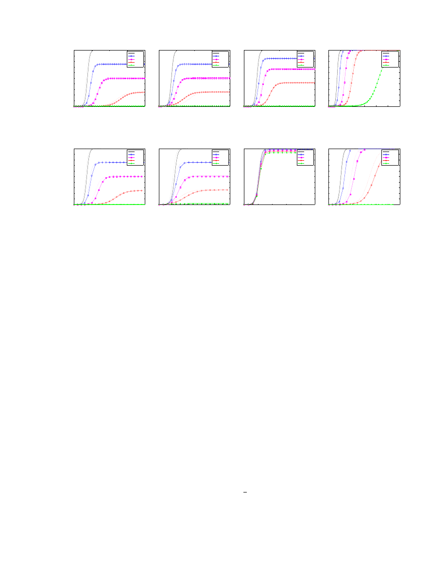
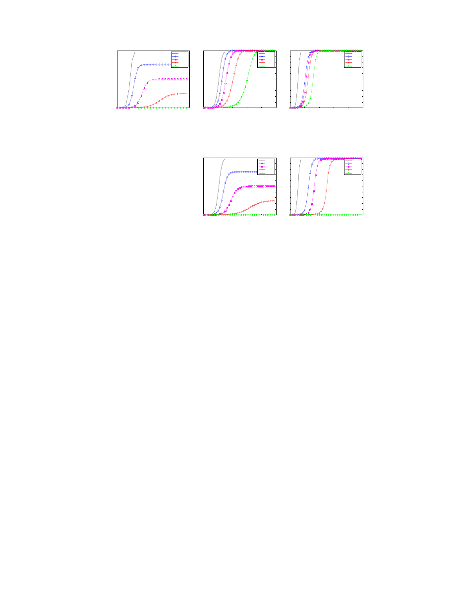
Figure 4 shows the effectiveness of the four strategies – Proactive Protection, Reactive Antibody Defense,

Reactive Address Blacklisting, and Local Containment– for defending against a CodeRed (a-d) and Slammer

(e-h) outbreak. Each graph shows the evolution of the infected host population based upon 5 different

incremental deployment (α) values: 0%, 25%, 50%, 75%, and 100%. The simulation results (solid lines in

the graph) confirm our theoretical formulas (dotted lines).

We see that under the simulation parameter, with Proactive Protection, Reactive Antibody Defense and

Reactive Address Blacklisting, very few participating hosts are infected in the measured time period even

with a small incremental deployment factor α. Note in the Proactive Protection scheme the slope is slightly

increasing, and eventually after a long time all hosts will be infected. We also see that increasing α for

Proactive Protection and Reactive Antibody Defense significantly decreases the total infected population.

Local Containment only slows down the worm propagation.

5.3

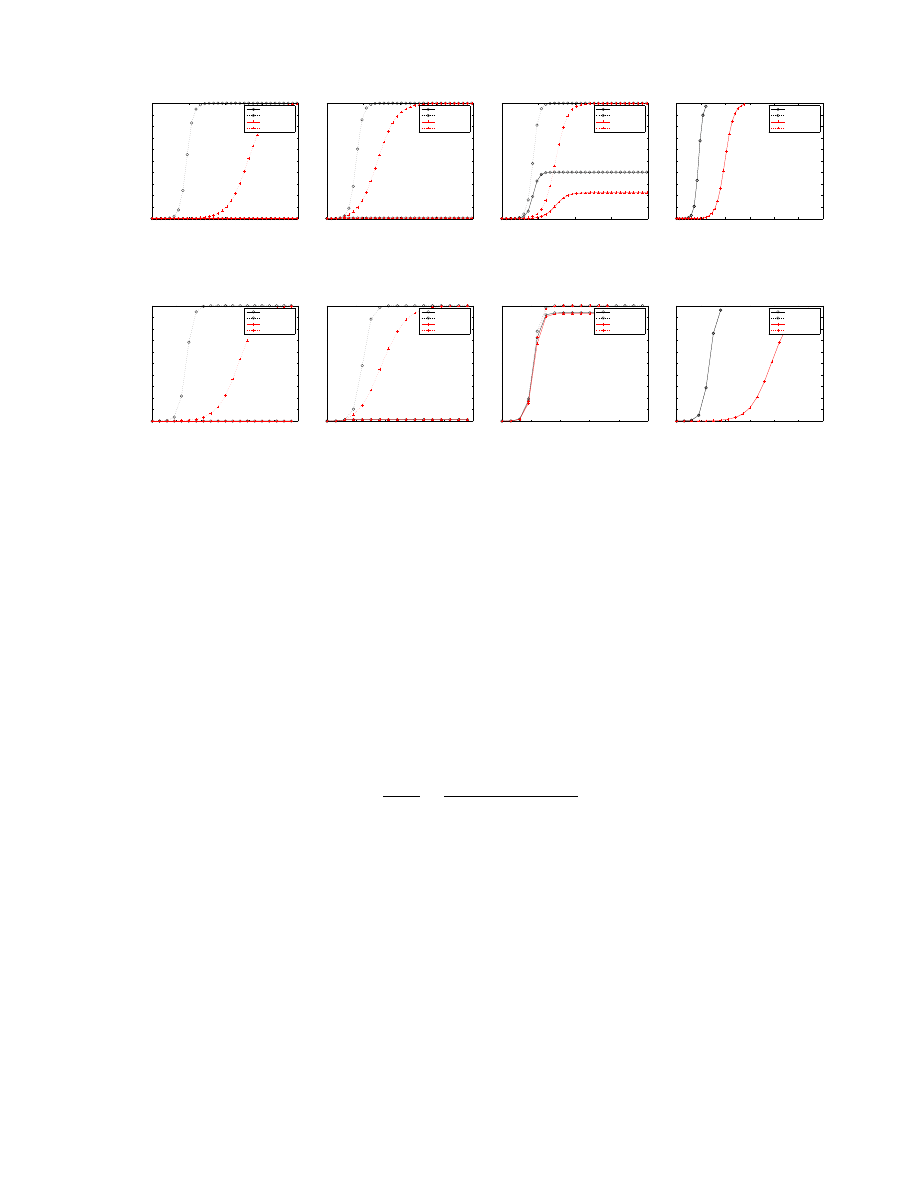
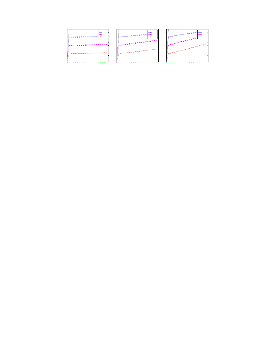
Overall vs. Participation Infection Factor Analysis

In order to understand how participation influences the infection factors, we evaluate both participation infec-

tion factor (PIF) and non-participation factor (NPIF) (as defined in Section 2) for two different deployment

ratios: 25% and 75%. Figure 5 shows the result of our theoretical analysis and simulation results for each

strategy.

With the CodeRed worm (Figure 5 a-d), participants of Reactive Antibody Defense are completely pro-

tected and Proactive Protection participants are protected within the time period measured (there is a very

slight upward slope in the graph that would continue to 100% with Proactive Protection), while all non-

participants all become infected. These results demonstrate a strong motivation for hosts to participate in

such strategies when possible. Reactive Address Blacklisting does an adequate job protecting participants,

with about 40% infected. Everyone in a Local Containment strategy is infected within the time period mea-

sured, with no noticeable benefit for participants.

Note that the contact rate β =

*scan rate.

500

1000

1500

2000

100

Time ( in minutes)

infected machines (%)

=0.25

=0.5

=0.75

(a) Proactive Protection

(C.R)

500

1000

1500

2000

100

Time ( in minutes)

infected machines (%)

=0.25

=0.5

=0.75

(b) Reactive Antibody

Defense (C.R)

500

1000

1500

2000

100

Time ( in minutes)

infected machines (%)

=0.25

=0.5

=0.75

Blacklisting (C.R)

500

1000

1500

2000

2500

3000

100

Time ( in minutes)

infected machines (%)

=0.25

=0.5

=0.75

(d) Local Containment

(C.R)

100

200

300

400

500

600

100

Time ( in seconds)

infected machines (%)

=0.25

=0.5

=0.75

(e) Proactive Protection

(S.L)

100

200

300

400

500

100

Time ( in seconds)

infected machines (%)

=0.25

=0.5

=0.75

(f) Reactive Antibody De-

fense (S.L)

100

200

300

400

500

100

Time ( in seconds)

infected machines (%)

=0.25

=0.5

=0.75

(g) Reactive Address

Blacklisting (S.L)

100

200

300

400

500

600

100

Time ( in seconds)

infected machines (%)

=0.25

=0.5

=0.75

(h) Local Containment

(S.L)

Figure 4: Partial Deployment Our simulation (solid lines) and theoretical (dotted lines) results for CodeRed

(top) and Slammer (bottom) random scanning worms for each defense strategy. Each graph shows the

infected host percentage over time for five different incremental deployment ratios (α). The theoretic pre-

dictions and experimental results match well.

The Slammer worm results (Figure 5 e-h) are similar to CodeRed for the Proactive Protection, Reac-

tive Antibody Defense, and Reactive Address Blacklisting strategies. Local Containment participants do

noticeably worse as the scan rate is much faster than the reaction time for adding hosts to the blacklist.

Comparison of Defense Strategies – Tomorrow’s Smart Worms

In this section we investigate smart worms that may appear in the future. We first design a new kind of

smart worm that targets Proactive Protection schemes, and analyze a proposed defense. We then use the

same parameters as Section 5, except we change the worm to use a hit-list instead of random scanning. A

hit-list worm knows a priori which hosts are vulnerable and does not waste time scanning non-vulnerable

hosts [25].

6.1

Brute-force worms

Our analysis so far has indicated Proactive Protection is an effective defense strategy. However, Proactive

Protection is vulnerable to a brute force attack in which a worm repeatedly attempts infection until a protected

host is infected. If Proactive Protection were deployed tomorrow, we should expect worms to take advantage

of this weakness.

We call worms that repeatedly attempt infection until success brute-force worms. With a uniform protec-

tion factor p, a brute-force worm will need to make about

1
p

infection attempts before succeeding. Figure 6(a)

shows the Proactive Protection defense against a normal Slammer worm outbreak, while Figure 6(b) shows

the effectiveness against a brute-force Slammer worm.

500

1000

1500

2000

100

↓

=0.25 (P.I.F.)

←

=0.25 (N.P.I.F.)

↓

=0.75 (P.I.F.)

←

=0.75 (N.P.I.F.)

Time ( in minutes)

infected machines (%)

=0.25 (P.I.F.)

=0.25(N.P.I.F)

=0.75 (P.I.F)

=0.75(N.P.I.F)

(a) Proactive Protection

(C.R)

500

1000

1500

2000

100

←

=0.25 (N.P.I.F.)

↓

=0.25 (P.I.F.)

←

=0.75 (N.P.I.F.)

↓

=0.75 (P.I.F.)

Time ( in minutes)

infected machines (%)

=0.25 (P.I.F.)

=0.25(N.P.I.F)

=0.75 (P.I.F)

=0.75(N.P.I.F)

(b) Reactive Antibody

Defense (C.R)

500

1000

1500

2000

100

←

=0.25 (N.P.I.F.)

←

=0.25 (P.I.F.)

←

=0.75 (N.P.I.F.)

←

=0.75 (P.I.F.)

Time ( in minutes)

infected machines (%)

=0.25 (P.I.F.)

=0.25(N.P.I.F)

=0.75 (P.I.F)

=0.75(N.P.I.F)

Blacklisting (C.R)

500

1000

1500

2000

2500

3000

100

←

=0.25 (P.I.F.)

←

=0.25 (N.P.I.F.)

←

=0.75 (P.I.F.)

←

=0.75 (N.P.I.F.)

Time ( in minutes)

infected machines (%)

=0.25 (P.I.F.)

=0.25(N.P.I.F)

=0.75 (P.I.F)

=0.75(N.P.I.F)

(d) Local Containment

(C.R)

100

200

300

400

500

600

100

↓

=0.25 (P.I.F.)

←

=0.25 (N.P.I.F.)

↓

=0.75 (P.I.F.)

←

=0.75 (N.P.I.F.)

Time ( in seconds)

infected machines (%)

=0.25 (P.I.F.)

=0.25(N.P.I.F)

=0.75 (P.I.F)

=0.75(N.P.I.F)

(e) Proactive Protection

(S.L)

100

200

300

400

500

100

↓

=0.25 (P.I.F.)

←

=0.25 (N.P.I.F.)

↓

=0.75 (P.I.F.)

←

=0.75 (N.P.I.F.)

Time ( in seconds)

infected machines (%)

=0.25 (P.I.F.)

=0.25(N.P.I.F)

=0.75 (P.I.F)

=0.75(N.P.I.F)

(f) Reactive Antibody De-

fense (S.L)

100

200

300

400

500

100

←

=0.25 (P.I.F.)

←

=0.25 (N.P.I.F.)

←

=0.75 (P.I.F.)

←

=0.75 (N.P.I.F.)

Time ( in seconds)

infected machines (%)

=0.25 (P.I.F.)

=0.25(N.P.I.F)

=0.75 (P.I.F)

=0.75(N.P.I.F)

(g) Reactive Address

Blacklisting (S.L)

100

200

300

400

500

600

100

←

=0.25 (P.I.F.)

←

=0.25 (N.P.I.F.)

←

=0.75 (P.I.F.)

←

=0.75 (N.P.I.F.)

Time ( in seconds)

infected machines (%)

=0.25 (P.I.F.)

=0.25(N.P.I.F)

=0.75 (P.I.F)

=0.75(N.P.I.F)

(h) Local Containment

(S.L)

Figure 5: Infection Factor Figures a-f show both the non-participation infection factor (NPIF) and participa-

tion infection factor (PIF) for CodeRed and Slammer random scanning worms.

We can make a brute force worm smarter by allowing all worms to share a global list of discovered vul-

nerable hosts. We call such a worm a Collaborative Brute-force Worm. Figure 6(c) shows the effectiveness

of Proactive Protection against a collaborative brute-force worm.

Hardened Proactive Protection.

We create a Hardened Proactive Protection to combat brute-force and

collaborative brute-force worms by augmenting each participating host a connection counter which is incre-

mented on each failed infection attempt from a host. When the counter exceeds a sensitivity threshold R, the

participating host no longer accepts new connections from that host.

We can derive the time evolution I(t) for Hardened Proactive Protection with full deployment against

the brute-force worm as:

dI(t)

βRpI(t)(N − I(t))

(29)

Figure 7 shows the effect of different sensitivity threshold values for the Hardened Proactive Protection

against the brute-force Slammer worm. For all R values the number of infections over the first 500 seconds

is about the same. After that, we see that smaller R values, i.e., the defense allows fewer failed infection

attempts from a host, results in a slower growth rate. Note that for a brute-force worm using hit-lists, the

defense result will be the same as shown in Figure 8 (a) & (e).

Figure 6(d-e) shows the result of Hardened Proactive Protection with R = 10 against a brute-force and

collaborative brute-force Slammer worm. Note this worm uses fast scanning, and coordinates via a master

global list of yet uninfected vulnerable hosts. Our results indicate Hardened Proactive Protection is effective

even against such smart worms.

100

200

300

400

500

600

100

Time ( in seconds)

infected machines (%)

=0.25

=0.5

=0.75

(a) Slammer vs. Proactive

Protection

200

400

600

800

1000

100

Time ( in seconds)

infected machines (%)

=0.25

=0.5

=0.75

(b) Brute force worm vs.

Proactive Protection

200

400

600

800

1000

100

Time ( in seconds)

infected machines (%)

=0.25

=0.5

=0.75

force worm vs. Proactive

Protection

200

400

600

800

1000

100

Time ( in seconds)

infected machines (%)

=0.25

=0.5

=0.75

(d) Brute force worm vs.

Hardened Proactive Pro-

tection

200

400

600

800

1000

100

Time ( in seconds)

infected machines (%)

=0.25

=0.5

=0.75

(e) Collaborative Brute

force worm vs. Hardened

Proactive Protection

Figure 6: (a) shows the Slammer worm outbreak is controlled by Proactive Protection as in Section 4. (b)

is a brute-force Slammer worm, which Proactive Protection can no longer control. (c) is a collaborative

brute-force Slammer worm, which is even faster than the normal brute-force worm. (d) and (e) shows the

hardened Proactive Protection strategy can control even the brute-force Slammer worm.

6.2

Hit-list Brute-force Worms

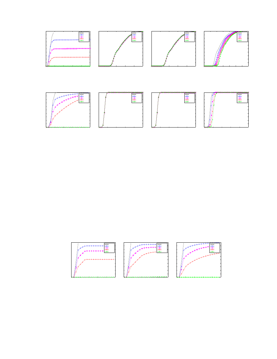
We analyze the effectiveness of each strategy against brute-force worms using a hit-list instead of random

scanning. A hit-list worm knows all vulnerable hosts a priori and only scans those hosts appearing on

the hit-list. Since infection is only attempted on vulnerable hosts, hit-list worms are one of the hardest to

control [25]. Note that we combine the hit-list worm with the collaborative brute-force worm described in

section 6.1 to make an even more aggressive worm against Proactive Protection.

Individual defense.

Figure 8 shows the effectiveness of each individual strategy against a hit-list version

of the brute-force Slammer and brute-force CodeRed worms, i.e., we use the same scanning rate as the

Slammer and CodeRed worms except that all scan attempts in the hit-list version will reach vulnerable hosts.

Reactive Antibody Defense and Reactive Address Blacklisting strategies have little effect for both hit-list

worms because the infection rate is faster than the reaction time values (δ

and δ

) we picked.

Due to the fast propagation speed of hit-list worms, implementations of these two strategies are not

likely to provide fast enough reaction time to be effective against hit-list worms. Local Containment is also

ineffective overall.

In this experiment, Proactive Protection clearly does the best job at controlling both worms. With

CodeRed, Proactive Protection controls the worm with even small deployment factors for the time period

measured (note there is a slight upward slope that would continue until 100% were infected), and further

maintains a near-zero percent infection with 100% deployment for the entire time period measured. With

Slammer, Proactive Protection delays infection for hosts much more substantially than the other defense

2000

4000

6000

8000

10000

100

Time ( in seconds)

infected machines (%)

=0.25

=0.5

=0.75

(a) R = 10

2000

4000

6000

8000

10000

100

Time ( in seconds)

infected machines (%)

=0.25

=0.5

=0.75

(b) R = 50

2000

4000

6000

8000

10000

100

Time ( in seconds)

infected machines (%)

=0.25

=0.5

=0.75

Figure 7: Effect of the sensitivity threshold on hardened Proactive Protection

approaches.

Hybrid defense.

Figure 9 presents brute-force Slammer worm using hit-list scanning for Proactive Protec-

tion hybrid defenses. To see the influence of the synergy, we change the reaction time of Reactive Antibody

Defense (δ

) to be 30 seconds, instead of the previous 60 seconds. The reaction time of Reactive Address

Blacklisting (δ

) remains 30 seconds. We do not show other defenses because the exact graph is too depen-

dent on the specific parameter choices to be meaningful.

The Proactive Protection + Reactive Antibody Defense hybrid provides the best protection of the consid-

ered schemes for both total effectiveness and largest gain as the partial deployment factor α increases. The

kinks in the graph (e.g., at t = 30 where α = 0.25, 0.5, and 0.75) show where Reactive Antibody Defense

takes over from Proactive Protection. Proactive Protection + Reactive Address Blacklisting performance is

not terrible in either respect, though clearly secondary. The smoother graph for Proactive Protection + Local

Containment is indicative of the trade-off between p and the scan rate threshold β

as discussed in Section 4.

Related Work

Moore et al. [14] is the most closely related work comparing defense systems. They analyze how the re-

action time for content filtering and address blacklisting influences the number of infected machines. Their

conclusion that reaction time is key for content filtering and blacklisting concurs with our results. Porras et.

al. analyze a hybrid approach that combines rate limiting and “friends” [20]. Their results show that hybrid

strategies do yield substantial improvements. Our work provides a more complete setting, along with more

general theoretic and simulation results.

Many people have proposed systems for automatically creating content filters [12, 13, 14, 17, 19, 23].

This line of work can benefit from our theoretical analysis.

Address space randomization as been proposed by [1, 4, 6, 8, 9, 28]. Shacham et al. show the overall

security of address randomization is suspect as a complete defense mechanism [21]. Our results, however,

show address randomization can be an effective tool because it can slow down extremely fast spreading

worms such as hit-list worms.

Zou models worm scan strategies using similar susceptible-infected models [29, 30]. Different worm

scanning strategies can be plugged in to our taxonomy.

Conclusion and Recommendations

We provide the first systematic study of worm defense systems. We created a taxonomy consisting of four

strategies: Proactive Protection, Reactive Antibody Defense, Reactive Address Blacklisting, Local Contain-

100

Time ( in minutes)

infected machines (%)

=0.25

=0.5

=0.75

(a) Proactive Protection

(C.R H.L.)

0.2

0.4

0.6

0.8

100

Time ( in minutes)

infected machines (%)

=0.25

=0.5

=0.75

(b) Reactive Antibody

Defense (C.R H.L.)

0.2

0.4

0.6

0.8

100

Time ( in minutes)

infected machines (%)

=0.25

=0.5

=0.75

Blacklisting (C.R H.L.)

0.2

0.4

0.6

0.8

1.2

1.4

100

Time ( in minutes)

infected machines (%)

=0.25

=0.5

=0.75

(d) Local Containment

(C.R H.L.)

100

Time ( in seconds)

infected machines (%)

=0.25

=0.5

=0.75

(e) Proactive Protection

(S.L H.L.)

100

Time ( in seconds)

infected machines (%)

=0.25

=0.5

=0.75

(f) Reactive Antibody De-

fense (S.L H.L.)

100

Time ( in seconds)

infected machines (%)

=0.25

=0.5

=0.75

(g) Reactive Address

Blacklisting (S.L H.L.)

100

Time ( in seconds)

infected machines (%)

=0.25

=0.5

=0.75

(h) Local Containment

(S.L H.L.)

Figure 8: Effectiveness evaluation against the hit-list worms

ment. Our taxonomy reveals for each strategy the key factors that determine its effectiveness, and we provide

theoretical analysis and simulation-based evaluation of the effectiveness of each defense category.

Our analysis also shows that the effectiveness of Local Containment requires very high deployment

ratio. Even if half of the internet deploys the defense, it can only slow down the worm propagation by

a factor of two. Thus, even though Local Containment may be a near-term approach in mitigating worm

attacks to a limited extend, it is not likely to be a long-term promising approach as it does not provide the

right deployment incentive and not strong defense.

Our analysis also shows that the effectiveness of Reactive Address Blacklisting is based on its reaction

time to be short. However, since each newly infected host needs to be put onto the (global) blacklist quickly

after it became infected, this offers a severe challenge to defend again fast-propagating worms. Thus, this

100

Time ( in seconds)

infected machines (%)

=0.25

=0.5

=0.75

(a) Proactive Protection

& Reactive Antibody De-

fense

100

Time ( in seconds)

infected machines (%)

=0.25

=0.5

=0.75

(b) Proactive Protection &

Reactive Address Black-

listing

100

Time ( in seconds)

infected machines (%)

=0.25

=0.5

=0.75

Local Containment

Figure 9: Hybrid defense against a Slammer worm using hit-list scanning with δ

= δ

30 seconds.

defense may be useful for slow-propagating worms, but is unlikely to be useful for fast-propagating worms.

Our analysis indicates a hybrid approach of Proactive Protection + Reactive Antibody Defense holds the

most promise for protecting against new ultra-fast smart worms. For example, TaintCheck [19, 18] proposes

using this hybrid combination. This hybrid is synergistic because Proactive Protection is a proactive, worm-

agnostic defense that can be deployed before an outbreak, while Reactive Antibody Defense provides an

eventual permanent fix once a worm is released.

Acknowledgement

The authors would like to thank Vern Paxson for his valuable discussion. The authors would like to thank

Nicholas Weaver for providing his source code of his simulator to enable us to build our own simulator for

the defense strategies described in this paper.

References

[1] PaX.

http://pax.grs

ec ur it y.n et /

[2] Elena Gabriela Barrantes, David H. Ackley, Stephanie Forrest, Trek S. Palmer, Darko Stefanovic, and

Dino Dai Zovi. Intrusion detection: Randomized instruction set emulation to disrupt binary code

injection attacks. In 10th ACM International Conference on Computer and Communications Security
(CCS)

, October 2003.

[3] Elena Gabriela Barrantes, David H. Ackley, Stephanie Forrest, and Darko Stefanovic. Randomized

instruction set emulation. ACM Transactions on Information and System Security, 8(1):3–40, 2005.

[4] Sandeep Bhatkar, Daniel C. DuVarney, and R. Sekar. Address obfuscation: An efficient approach to

combat a broad range of memory error exploits. In Proceedings of 12th USENIX Security Symposium,

2003.

[5] Sandeep Bhatkar, R. Sekar, and Daniel C. DuVarney. Efficient techniques for comprehensive protection

from memory error exploits. In Proceedings of the 14th USENIX Security Symposium, 2005.

[6] Monica Chew and Dawn Song. Mitigating buffer overflows by operating system randomization. Tech-

nical report, Carnegie Mellon University, 2002.

[7] Crispin Cowan, Steve Beattie, John Johansen, and Perry Wagle. Pointguard: Protecting pointers from

buffer overflow vulnerabilities. In Proceedings of the 12th USENIX Security Symposium, 2003.

[8] Daniel C. DuVarney, R. Sekar, and Yow-Jian Lin. Benign software mutations: A novel approach to

protect against large-scale network attacks. Center for Cybersecurity White Paper, October 2002.

[9] Stephanie Forrest, Anil Somayaji, and David H. Ackley. Building diverse computer systems. In Pro-

ceedings of 6th workshop on Hot Topics in Operating Systems

, 1997.

[10] Herbert W. Hethcote. The Mathematics of Infectious Diseases. SIAM Review, 42(4):599–653, 2000.

[11] Gaurav S. Kc, Angeles D. Keromytis, and Vassilis Prevelakis. Countering code-injection attacks with

instruction-set randomization. In 10th ACM International Conference on Computer and Communica-
tions Security (CCS)

, October 2003.

[12] Hyang-Ah Kim and Brad Karp. Autograph: toward automated, distributed worm signature detection.

In Proceedings of the 13th USENIX Security Symposium, August 2004.

[13] Christian Kreibich and Jon Crowcroft. Honeycomb - creating intrusion detection signatures using

honeypots. In Proceedings of the Second Workshop on Hot Topics in Networks (HotNets-II), November

2003.

[14] David Moore, Vern Paxson, Colleen Shannon, Geoffrey M. Voelker, and Stefan Savage. Internet quar-

antine: Requirements for containing self-propagating code. In Proceedings of IEEE INFOCOM, March

2003.

[15] David Moore, Stefan Savage, Colleen Shannon, Stuart Staniford, and Nicholas Weaver. Inside the

Slammer worm. IEEE Security and Privacy, July 2003.

[16] David Moore, Colleen Shannon, and Jeffery Brown. Code-Red: a case study on the spread and vic-

tims of an internet worm. In Proceedings of ACM/USENIX Internet Measurement Workshop, France,

November 2002.

[17] James Newsome, Brad Karp, and Dawn Song. Polygraph: Automatically generating signatures for

polymorphic worms. In Proceedings of the IEEE Symposium on Security and Privacy, May 2005.

[18] James Newsome and Dawn Song. Dynamic taint analysis for automatic detection, analysis, and sig-

nature generation of exploits on commodity software. Technical Report CMU-CS-04-140, Carnegie

Mellon University, 2004.

[19] James Newsome and Dawn Song. Dynamic taint analysis for automatic detection, analysis, and sig-

nature generation of exploits on commodity software. In Proceedings of the 12th Annual Network and
Distributed Systems Security Symposium

, February 2005.

[20] Phillip Porras, Linda Briesemeister, Keith Skinner, Karl Levitt, Jeff Rowe, and Yu-Cheng Allen Ting.

A hybrid quarantine defense. In Proceedings of the 2004 ACM Workshop on Rapid Malcode (WORM),

Washington, DC, USA, 2004.

[21] Hovav Shacham, Matthew Page, Ben Pfaff, Eu-Jin Goh, Nagendra Modadugu, and Dan Boneh. On

the effectiveness of address-space randomization. In Proceedings of the 11th ACM Conference on
Computer and Communications Security

, October 2004.

[22] Stelios Sidiroglou and Angelos D. Keromytis. Countering network worms through automatic patch

generation. In Proceedings of IEEE Symposium on Security and Privacy, 2005.

[23] Sumeet Singh, Cristian Estan, George Varghese, and Stefan Savage. Automated worm fingerprinting.

In Proceedings of the 6th ACM/USENIX Symposium on Operating System Design and Implementation
(OSDI)

, December 2004.

[24] Nora Sovarel, David Evans, and Nathanael Paul. Where’s the feeb? the effectiveness of instruction set

randomization. In 14th USENIX Security Symposium, August 2005.

[25] Stuart Staniford, Vern Paxson, and Nicholas Weaver. How to 0wn the internet in your spare time. In

Proceedings of 11th USENIX Security Symposium

, August 2002.

[26] Jamie Twycross and Matthew M. Williamson. Implementing and testing a virus throttle. In Proceedings

of 12th USENIX Security Symposium

, August 2003.

[27] Matthew M. Williamson. Throttling viruses: Restricting propagation to defeat malicious mobile code.

In Proceedings of the 18th Annual Computer Security Applications Conference, 2002.

[28] Jun Xu, Zbigniew Kalbarczyk, and Ravishankar K. Iyer. Transparent runtime randomization for secu-

rity. Technical report, Center for Reliable and Higher Performance Computing, University of Illinois

at Urbana-Champaign, May 2003.

[29] Cliff Zou, Weibo Gong, Don Towsley, and Lixin Gao. The monitoring and early detection of internet

worms. IEEE/ACM Transaction on Networking, To appear.

[30] Cliff Zou, Don Towsley, and Weibo Gong. On the performance of internet worm scanning strategies.

Journal of Performance Evaluation

, To appear.

Wyszukiwarka

Podobne podstrony:
Multiscale Modeling and Simulation of Worm Effects on the Internet Routing Infrastructure
Possible Effects of Strategy Instruction on L1 and L2 Reading
53 755 765 Effect of Microstructural Homogenity on Mechanical and Thermal Fatique
31 411 423 Effect of EAF and ESR Technologies on the Yield of Alloying Elements
21 269 287 Effect of Niobium and Vanadium as an Alloying Elements in Tool Steels
Effects of the Great?pression on the U S and the World
Effect of caffeine on fecundity egg laying capacity development time and longevity in Drosophila
Effects Of 20 H Rule And Shield Nieznany
Effect of Drugs and Alcohol on Teenagers
A systematic review and meta analysis of the effect of an ankle foot orthosis on gait biomechanics a
Effect of heat treatment on microstructure and mechanical properties of cold rolled C Mn Si TRIP
71 1021 1029 Effect of Electron Beam Treatment on the Structure and the Properties of Hard
53 755 765 Effect of Microstructural Homogenity on Mechanical and Thermal Fatique
EFFECTS OF EATING AND NOT EATING ON ENERGY STORES AND BODY WEIGHT
Glińska, Sława i inni The effect of EDTA and EDDS on lead uptake and localization in hydroponically
Ecological effects of soil compaction and initial recovery dynamics a preliminary study
Abstract Synergistic Antifungal Effect of Lactoferrin with Azole Antifungals against Candida albican

więcej podobnych podstron