Haurie A , An Introduction to Dynamic Games Lctn

An Introduction to Dynamic Games

A. Haurie

J. Krawczyk

March 28, 2000

Contents

Foreword

1.1

What are Dynamic Games? . . . . . . . . . . . . . . . . . . . . . . .

1.2

Origins of these Lecture Notes . . . . . . . . . . . . . . . . . . . . .

1.3

Motivation . . . . . . . . . . . . . . . . . . . . . . . . . . . . . . .

Elements of Classical Game Theory

Decision Analysis with Many Agents

2.1

The Basic Concepts of Game Theory . . . . . . . . . . . . . . . . . .

2.2

Games in Extensive Form . . . . . . . . . . . . . . . . . . . . . . . .

2.2.1

Description of moves, information and randomness . . . . . .

2.2.2

Comparing Random Perspectives

. . . . . . . . . . . . . . .

2.3

Additional concepts about information . . . . . . . . . . . . . . . . .

2.3.1

Complete and perfect information . . . . . . . . . . . . . . .

2.3.2

Commitment . . . . . . . . . . . . . . . . . . . . . . . . . .

2.3.3

Binding agreement . . . . . . . . . . . . . . . . . . . . . . .

2.4

Games in Normal Form

. . . . . . . . . . . . . . . . . . . . . . . .

CONTENTS

2.4.1

Playing games through strategies . . . . . . . . . . . . . . . .

2.4.2

From the extensive form to the strategic or normal form

. . .

2.4.3

Mixed and Behavior Strategies . . . . . . . . . . . . . . . . .

Solution concepts for noncooperative games

3.1

introduction . . . . . . . . . . . . . . . . . . . . . . . . . . . . . . .

3.2

Matrix Games . . . . . . . . . . . . . . . . . . . . . . . . . . . . . .

3.2.1

Saddle-Points . . . . . . . . . . . . . . . . . . . . . . . . . .

3.2.2

Mixed strategies . . . . . . . . . . . . . . . . . . . . . . . .

3.2.3

Algorithms for the Computation of Saddle-Points . . . . . . .

3.3

Bimatrix Games . . . . . . . . . . . . . . . . . . . . . . . . . . . . .

3.3.1

Nash Equilibria . . . . . . . . . . . . . . . . . . . . . . . . .

3.3.2

Shortcommings of the Nash equilibrium concept . . . . . . .

3.3.3

Algorithms for the Computation of Nash Equilibria in Bima-
trix Games . . . . . . . . . . . . . . . . . . . . . . . . . . .

3.4

Concave

m-Person Games . . . . . . . . . . . . . . . . . . . . . . .

3.4.1

Existence of Coupled Equilibria . . . . . . . . . . . . . . . .

3.4.2

Normalized Equilibria . . . . . . . . . . . . . . . . . . . . .

3.4.3

Uniqueness of Equilibrium . . . . . . . . . . . . . . . . . . .

3.4.4

A numerical technique . . . . . . . . . . . . . . . . . . . . .

3.4.5

A variational inequality formulation . . . . . . . . . . . . . .

3.5

Cournot equilibrium . . . . . . . . . . . . . . . . . . . . . . . . . . .

3.5.1

The static Cournot model . . . . . . . . . . . . . . . . . . . .

CONTENTS

3.5.2

Formulation of a Cournot equilibrium as a nonlinear comple-
mentarity problem . . . . . . . . . . . . . . . . . . . . . . .

3.5.3

Computing the solution of a classical Cournot model . . . . .

3.6

Correlated equilibria . . . . . . . . . . . . . . . . . . . . . . . . . .

3.6.1

Example of a game with correlated equlibria

. . . . . . . . .

3.6.2

A general definition of correlated equilibria . . . . . . . . . .

3.7

Bayesian equilibrium with incomplete information

. . . . . . . . . .

3.7.1

Example of a game with unknown type for a player . . . . . .

3.7.2

Reformulation as a game with imperfect information . . . . .

3.7.3

A general definition of Bayesian equilibria

. . . . . . . . . .

3.8

Appendix on Kakutani Fixed-point theorem . . . . . . . . . . . . . .

3.9

exercises . . . . . . . . . . . . . . . . . . . . . . . . . . . . . . . . .

Repeated and sequential Games

Repeated games and memory strategies

4.1

Repeating a game in normal form

. . . . . . . . . . . . . . . . . . .

4.1.1

Repeated bimatrix games . . . . . . . . . . . . . . . . . . . .

4.1.2

Repeated concave games . . . . . . . . . . . . . . . . . . . .

4.2

Folk theorem . . . . . . . . . . . . . . . . . . . . . . . . . . . . . .

4.2.1

Repeated games played by automata . . . . . . . . . . . . . .

4.2.2

Minimax point . . . . . . . . . . . . . . . . . . . . . . . . .

4.2.3

Set of outcomes dominating the minimax point . . . . . . . .

4.3

Collusive equilibrium in a repeated Cournot game . . . . . . . . . . .

CONTENTS

4.3.1

Finite vs infinite horizon . . . . . . . . . . . . . . . . . . . .

4.3.2

A repeated stochastic Cournot game with discounting and im-
perfect information . . . . . . . . . . . . . . . . . . . . . . .

4.4

Exercises . . . . . . . . . . . . . . . . . . . . . . . . . . . . . . . .

Shapley’s Zero Sum Markov Game

5.1

Process and rewards dynamics . . . . . . . . . . . . . . . . . . . . .

5.2

Information structure and strategies

. . . . . . . . . . . . . . . . . .

5.2.1

The extensive form of the game . . . . . . . . . . . . . . . .

5.2.2

Strategies . . . . . . . . . . . . . . . . . . . . . . . . . . . .

5.3

Shapley’s-Denardo operator formalism . . . . . . . . . . . . . . . . .

5.3.1

Dynamic programming operators

. . . . . . . . . . . . . . .

5.3.2

Existence of sequential saddle points

. . . . . . . . . . . . .

Nonzero-sum Markov and Sequential games

6.1

Sequential Game with Discrete state and action sets . . . . . . . . . .

6.1.1

Markov game dynamics . . . . . . . . . . . . . . . . . . . .

6.1.2

Markov strategies . . . . . . . . . . . . . . . . . . . . . . . .

6.1.3

Feedback-Nash equilibrium . . . . . . . . . . . . . . . . . .

6.1.4

Sobel-Whitt operator formalism . . . . . . . . . . . . . . . .

6.1.5

Existence of Nash-equilibria . . . . . . . . . . . . . . . . . .

6.2

Sequential Games on Borel Spaces . . . . . . . . . . . . . . . . . . .

6.2.1

Description of the game . . . . . . . . . . . . . . . . . . . .

6.2.2

Dynamic programming formalism . . . . . . . . . . . . . . .

CONTENTS

6.3

Application to a Stochastic Duopoloy Model . . . . . . . . . . . . . .

6.3.1

A stochastic repeated duopoly . . . . . . . . . . . . . . . . .

6.3.2

A class of trigger strategies based on a monitoring device . . .

6.3.3

Interpretation as a communication device . . . . . . . . . . .

III

Differential games

Controlled dynamical systems

101

7.1

A capital accumulation process . . . . . . . . . . . . . . . . . . . . . 101

7.2

State equations for controlled dynamical systems . . . . . . . . . . . 102

7.2.1

Regularity conditions . . . . . . . . . . . . . . . . . . . . . . 102

7.2.2

The case of stationary systems . . . . . . . . . . . . . . . . . 102

7.2.3

The case of linear systems . . . . . . . . . . . . . . . . . . . 103

7.3

Feedback control and the stability issue . . . . . . . . . . . . . . . . 103

7.3.1

Feedback control of stationary linear systems . . . . . . . . . 104

7.3.2

stabilizing a linear system with a feedback control

. . . . . . 104

7.4

Optimal control problems . . . . . . . . . . . . . . . . . . . . . . . . 104

7.5

A model of optimal capital accumulation . . . . . . . . . . . . . . . . 104

7.6

The optimal control paradigm

. . . . . . . . . . . . . . . . . . . . . 105

7.7

The Euler equations and the Maximum principle . . . . . . . . . . . . 106

7.8

An economic interpretation of the Maximum Principle . . . . . . . . 108

7.9

Synthesis of the optimal control

. . . . . . . . . . . . . . . . . . . . 109

7.10 Dynamic programming and the optimal feedback control . . . . . . . 109

CONTENTS

7.11 Competitive dynamical systems

. . . . . . . . . . . . . . . . . . . . 110

7.12 Competition through capital accumulation . . . . . . . . . . . . . . . 110

7.13 Open-loop differential games . . . . . . . . . . . . . . . . . . . . . . 110

7.13.1 Open-loop information structure . . . . . . . . . . . . . . . . 110

7.13.2 An equilibrium principle . . . . . . . . . . . . . . . . . . . . 110

7.14 Feedback differential games . . . . . . . . . . . . . . . . . . . . . . 111

7.14.1 Feedback information structure

. . . . . . . . . . . . . . . . 111

7.14.2 A verification theorem . . . . . . . . . . . . . . . . . . . . . 111

7.15 Why are feedback Nash equilibria outcomes different from Open-loop

Nash outcomes? . . . . . . . . . . . . . . . . . . . . . . . . . . . . . 111

7.16 The subgame perfectness issue . . . . . . . . . . . . . . . . . . . . . 111

7.17 Memory differential games . . . . . . . . . . . . . . . . . . . . . . . 111

7.18 Characterizing all the possible equilibria . . . . . . . . . . . . . . . . 111

A Differential Game Model

113

7.19 A Game of R&D Investment . . . . . . . . . . . . . . . . . . . . . . 115

7.19.1 Dynamics of

R&D competition . . . . . . . . . . . . . . . . 115

7.19.2 Product Differentiation . . . . . . . . . . . . . . . . . . . . . 116

7.19.3 Economics of innovation . . . . . . . . . . . . . . . . . . . . 117

7.20 Information structure . . . . . . . . . . . . . . . . . . . . . . . . . . 118

7.20.1 State variables

. . . . . . . . . . . . . . . . . . . . . . . . . 118

7.20.2 Piecewise open-loop game. . . . . . . . . . . . . . . . . . . . 118

7.20.3 A Sequential Game Reformulation . . . . . . . . . . . . . . . 118

Chapter 1

Foreword

1.1

What are Dynamic Games?

Dynamic Games are mathematical models of the interaction between different agents
who are controlling a dynamical system. Such situations occur in many instances like
armed conflicts (e.g. duel between a bomber and a jet fighter), economic competition
(e.g. investments in R&D for computer companies), parlor games (Chess, Bridge).
These examples concern dynamical systems since the actions of the agents (also called
players) influence the evolution over time of the state of a system (position and velocity
of aircraft, capital of know-how for Hi-Tech firms, positions of remaining pieces on a
chess board, etc). The difficulty in deciding what should be the behavior of these
agents stems from the fact that each action an agent takes at a given time will influence
the reaction of the opponent(s) at later time. These notes are intended to present the
basic concepts and models which have been proposed in the burgeoning literature on
game theory for a representation of these dynamic interactions.

1.2

Origins of these Lecture Notes

These notes are based on several courses on Dynamic Games taught by the authors,
in different universities or summer schools, to a variety of students in engineering,
economics and management science. The notes use also some documents prepared in
cooperation with other authors, in particular B. Tolwinski [Tolwinski, 1988].

These notes are written for control engineers, economists or management scien-

tists interested in the analysis of multi-agent optimization problems, with a particular

CHAPTER 1. FOREWORD

emphasis on the modeling of conflict situations. This means that the level of mathe-
matics involved in the presentation will not go beyond what is expected to be known by
a student specializing in control engineering, quantitative economics or management
science. These notes are aimed at last-year undergraduate, first year graduate students.

The Control engineers will certainly observe that we present dynamic games as an

extension of optimal control whereas economists will see also that dynamic games are
only a particular aspect of the classical theory of games which is considered to have
been launched in [Von Neumann & Morgenstern 1944]. Economic models of imper-
fect competition, presented as variations on the ”classic” Cournot model [Cournot, 1838],
will serve recurrently as an illustration of the concepts introduced and of the theories
developed. An interesting domain of application of dynamic games, which is described
in these notes, relates to environmental management. The conflict situations occur-
ring in fisheries exploitation by multiple agents or in policy coordination for achieving
global environmental control (e.g. in the control of a possible global warming effect)
are well captured in the realm of this theory.

The objects studied in this book will be dynamic. The term dynamic comes from

Greek dynasthai (which means to be able) and refers to phenomena which undergo
a time-evolution. In these notes, most of the dynamic models will be discrete time.
This implies that, for the mathematical description of the dynamics, difference (rather
than differential) equations will be used. That, in turn, should make a great part of the
notes accessible, and attractive, to students who have not done advanced mathematics.
However, there will still be some developments involving a continuous time description
of the dynamics and which have been written for readers with a stronger mathematical
background.

1.3

Motivation

There is no doubt that a course on dynamic games suitable for both control engineer-
ing students and economics or management science students requires a specialized
textbook.

Since we emphasize the detailed description of the dynamics of some specific sys-

tems controlled by the players we have to present rather sophisticated mathematical
notions, related to control theory. This presentation of the dynamics must be accom-
panied by an introduction to the specific mathematical concepts of game theory. The
originality of our approach is in the mixing of these two branches of applied mathe-
matics.

There are many good books on classical game theory. A nonexhaustive list in-

1.3. MOTIVATION

cludes [Owen, 1982], [Shubik, 1975a], [Shubik, 1975b], [Aumann, 1989], and more
recently [Friedman 1986] and [Fudenberg & Tirole, 1991]. However, they do not in-
troduce the reader to the most general dynamic games. [Bas¸ar & Olsder, 1982] does
cover extensively the dynamic game paradigms, however, readers without a strong
mathematical background will probably find that book difficult. This text is therefore
a modest attempt to bridge the gap.

CHAPTER 1. FOREWORD

Part I

Elements of Classical Game Theory

Chapter 2

Decision Analysis with Many Agents

As we said in the introduction to these notes dynamic games constitute a subclass
of the mathematical models studied in what is usually called the classical theory of
game. It is therefore proper to start our exposition with those basic concepts of game
theory which provide the fundamental tread of the theory of dynamic games. For
an exhaustive treatment of most of the definitions of classical game theory see e.g.
[Owen, 1982], [Shubik, 1975a], [Friedman 1986] and [Fudenberg & Tirole, 1991].

2.1

The Basic Concepts of Game Theory

In a game we deal with the following concepts

• Players. They will compete in the game. Notice that a player may be an indi-

vidual, a set of individuals (or a team , a corporation, a political party, a nation,
a pilot of an aircraft, a captain of a submarine, etc. .

• A move or a decision will be a player’s action. Also, borrowing a term from

control theory, a move will be realization of a player’s control or, simply, his
control.

• A player’s (pure) strategy will be a rule (or function) that associates a player’s

move with the information available to him

at the time when he decides which

move to choose.

Political correctness promotes the usage of gender inclusive pronouns “they” and “their”. However,

in games, we will frequently have to address an individual player’s action and distinguish it from a
collective action taken by a set of several players. As far as we know, in English, this distinction is
only possible through usage of the traditional grammar gender exclusive pronouns: possessive “his”,
“her” and personal “he”, “she”. We find that the traditional grammar better suits your purpose (to avoid)

CHAPTER 2. DECISION ANALYSIS WITH MANY AGENTS

• A player’s mixed strategy is a probability measure on the player’s space of pure

strategies. In other words, a mixed strategy consists of a random draw of a pure
strategy. The player controls the probabilities in this random experiment.

• A player’s behavioral strategy is a rule which defines a random draw of the ad-

missible move as a function of the information available

. These strategies are

intimately linked with mixed strategies and it has been proved early [Kuhn, 1953]
that, for many games the two concepts coincide.

• Payoffs are real numbers measuring desirability of the possible outcomes of the

game, e.g. , the amounts of money the players may win (or loose). Other names
of payoffs can be: rewards, performance indices or criteria, utility measures,
etc. .

The concepts we have introduced above are described in relatively imprecise terms.
A more rigorous definition can be given if we set the theory in the realm of decision
analysis where decision trees give a representation of the dependence of outcomes on
actions and uncertainties . This will be called the extensive form of a game.

2.2

Games in Extensive Form

A game in extensive form is a graph (i.e. a set of nodes and a set of arcs) which has the
structure of a tree

and which represents the possible sequence of actions and random

perturbations which influence the outcome of a game played by a set of players.

2.2.1

Description of moves, information and randomness

A game in extensive form is described by a set of players, including one particular
player called Nature , and a set of positions described as nodes on a tree structure. At
each node one particular player has the right to move, i.e. he has to select a possible
action in an admissible set represented by the arcs emanating from the node.

The information at the disposal of each player at the nodes where he has to select

an action is described by the information structure of the game . In general the player

confusion and we will refer in this book to a singular genderless agent as “he” and the agent’s possession
as “his”.

A similar concept has been introduced in control theory under the name of relaxed controls.

A tree is a graph where all nodes are connected but there are no cycles. In a tree there is a single

node without ”parent”, called the ”root” and a set of nodes without descendants, the ”leaves”. There is
always a single path from the root to any leaf.

2.2. GAMES IN EXTENSIVE FORM

may not know exactly at which node of the tree structure the game is currently located.
His information has the following form:

he knows that the current position of the game is an element in a given
subset of nodes. He does not know which specific one it is.

When the player selects a move, this correponds to selecting an arc of the graph which
defines a transition to a new node, where another player has to select his move, etc.
Among the players, Nature is playing randomly, i.e. Nature’s moves are selected at
random. The game has a stopping rule described by terminal nodes of the tree. Then
the players are paid their rewards, also called payoffs .

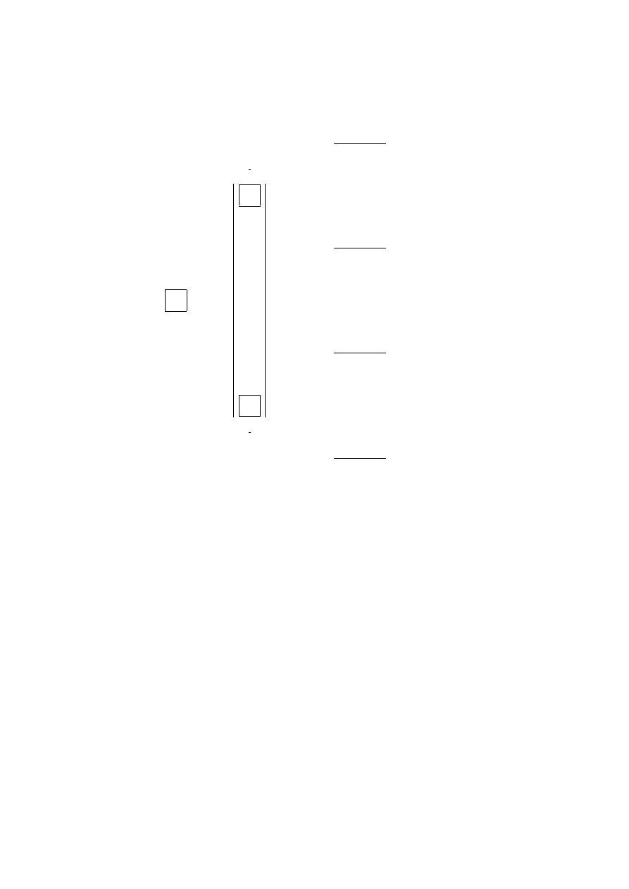
Figure 2.1 shows the extensive form of a two-player, one-stage stochastic game

with simultaneous moves. We also say that this game has the simultaneous move in-
formation structure . It corresponds to a situation where Player 2 does not know which
action has been selected by Player 1 and vice versa. In this figure the node marked

corresponds to the move of player 1, the nodes marked

correspond to the move of

Player 2.

The information of the second player is represented by the oval box. Therefore

Player 2 does not know what has been the action chosen by Player 1. The nodes
marked

E correspond to Nature’s move. In that particular case we assume that three

possible elementary events are equiprobable. The nodes represented by dark circles
are the terminal nodes where the game stops and the payoffs are collected.

This representation of games is obviously inspired from parlor games like Chess ,

Poker , Bridge , etc which can be, at least theoretically, correctly described in this
framework. In such a context, the randomness of Nature ’s play is the representation
of card or dice draws realized in the course of the game.

The extensive form provides indeed a very detailed description of the game. It is

however rather non practical because the size of the tree becomes very quickly, even
for simple games, absolutely huge. An attempt to provide a complete description of a
complex game like Bridge , using an extensive form, would lead to a combinatorial ex-
plosion. Another drawback of the extensive form description is that the states (nodes)
and actions (arcs) are essentially finite or enumerable. In many models we want to deal
with, actions and states will also often be continuous variables. For such models, we
will need a different method of problem description.

Nevertheless extensive form is useful in many ways. In particular it provides the

fundamental illustration of the dynamic structure of a game. The ordering of the se-
quence of moves, highlighted by extensive form, is present in most games. Dynamic
games theory is also about sequencing of actions and reactions. Here, however, dif-

CHAPTER 2. DECISION ANALYSIS WITH MANY AGENTS

1/3

[payoffs]

1/3

[payoffs]

1/3

[payoffs]

1/3

[payoffs]

Figure 2.1: A game in extensive form

ferent mathematical tools are used for the representation of the game dynamics. In
particular, differential and/or difference equations are utilized for this purpose.

2.2.2

Comparing Random Perspectives

Due to Nature’s randomness, the players will have to compare and choose among
different random perspectives in their decision making. The fundamental decision
structure is described in Figure 2.2. If the player chooses action

he faces a random

perspective of expected value 100. If he chooses action

he faces a sure gain of 100.

If the player is risk neutral he will be indifferent between the two actions. If he is risk

2.2. GAMES IN EXTENSIVE FORM

averse he will choose action

, if he is risk lover he will choose action

. In order to

e.v.=100

1/3

100

200

Figure 2.2: Decision in uncertainty

represent the attitude toward risk of a decision maker Von Neumann and Morgenstern
introduced the concept of cardinal utility [Von Neumann & Morgenstern 1944]. If one
accepts the axioms of utility theory then a rational player should take the action which
leads toward the random perspective with the highest expected utility .

This solves the problem of comparing random perspectives. However this also

introduces a new way to play the game. A player can set a random experiment in order
to generate his decision. Since he uses utility functions the principle of maximization
of expected utility permits him to compare deterministic action choices with random
ones.

As a final reminder of the foundations of utility theory let’s recall that the Von Neumann-

Morgenstern utility function is defined up to an affine transformation. This says that
the player choices will not be affected if the utilities are modified through an affine
transformation.

CHAPTER 2. DECISION ANALYSIS WITH MANY AGENTS

2.3

Additional concepts about information

What is known by the players who interact in a game is of paramount importance. We
refer briefly to the concepts of complete and perfect information.

2.3.1

Complete and perfect information

The information structure of a game indicates what is known by each player at the time
the game starts and at each of his moves.

Complete vs Incomplete Information

Let us consider first the information available to the players when they enter a game
play. A player has complete information if he knows

• who the players are

• the set of actions available to all players

• all possible outcomes to all players.

A game with complete information and common knowledge is a game where all play-
ers have complete information and all players know that the other players have com-
plete information.

Perfect vs Imperfect Information

We consider now the information available to a player when he decides about specific
move. In a game defined in its extensive form, if each information set consists of just
one node, then we say that the players have perfect information . If that is not the case
the game is one of imperfect information .

Example 2.3.1 A game with simultaneous moves, as e.g. the one shown in Figure 2.1,
is of imperfect information.

2.4. GAMES IN NORMAL FORM

Perfect recall

If the information structure is such that a player can always remember all past moves
he has selected, and the information he has received, then the game is one of perfect
recall . Otherwise it is one of imperfect recall .

2.3.2

Commitment

A commitment is an action taken by a player that is binding on him and that is known
to the other players. In making a commitment a player can persuade the other players
to take actions that are favorable to him. To be effective commitments have to be
credible . A particular class of commitments are threats .

2.3.3

Binding agreement

Binding agreements are restrictions on the possible actions decided by two or more
players, with a binding contract that forces the implementation of the agreement. Usu-
ally, to be binding an agreement requires an outside authority that can monitor the
agreement at no cost and impose on violators sanctions so severe that cheating is pre-
vented.

2.4

Games in Normal Form

2.4.1

Playing games through strategies

Let

M =

{1, . . . , m} be the set of players. A pure strategy γ

for Player

j is a mapping

which transforms the information available to Player

j at a decision node where he is

making a move into his set of admissible actions. We call strategy vector the

m-tuple

γ = (γ)

j=1,...m

. Once a strategy is selected by each player, the strategy vector

γ is

defined and the game is played as it were controlled by an automaton

An outcome (expressed in terms of expected utility to each player if the game

includes chance nodes) is associated with a strategy vector

γ. We denote by Γ

the set

This idea of playing games through the use of automata will be discussed in more details when we

present the folk theorem for repeated games in Part II

CHAPTER 2. DECISION ANALYSIS WITH MANY AGENTS

of strategies for Player

j. Then the game can be represented by the m mappings

: Γ

× · · · Γ

→ IR, j ∈ M

that associate a unique (expected utility) outcome

(γ) for each player j

∈ M with

a given strategy vector in

∈ Γ

× · · · Γ

. One then says that the game is

defined in its normal form .

2.4.2

From the extensive form to the strategic or normal form

We consider a simple two-player game, called “matching pennies”. The rules of the
game are as follows:

The game is played over two stages. At first stage each player chooses
head (H) or tail (T) without knowing the other player’s choice. Then they
reveal their choices to one another. If the coins do not match, Player 1
wins $5 and Payer 2 wins -$5. If the coins match, Player 2 wins $5 and
Payer 1 wins -$5. At the second stage, the player who lost at stage 1 has
the choice of either stopping the game or playing another penny matching
with the same type of payoffs as in the first stage (Q, H, T).

The extensive form tree

This game is represented in its extensive form in Figure 2.3. The terminal payoffs rep-
resent what Player 1 wins; Player 2 receives the opposite values. We have represented
the information structure in a slightly different way here. A dotted line connects the
different nodes forming an information set for a player. The player who has the move
is indicated on top of the graph.

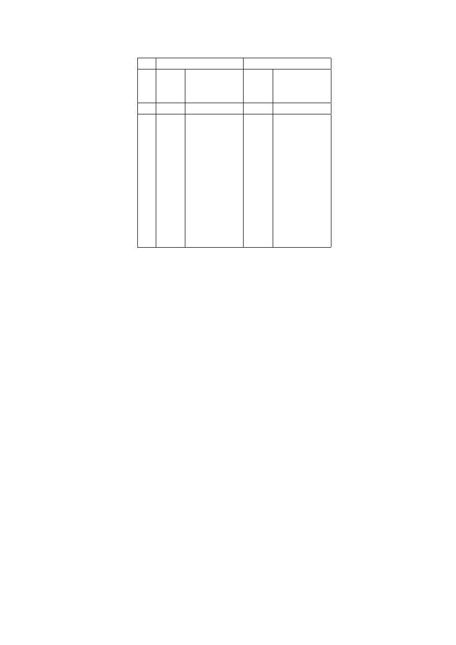
Listing all strategies

In Table 2.1 we have identified the 12 different strategies that can be used by each of
the two players in the game of Matching pennies. Each player moves twice. In the
first move the players have no information; in the second move they know what have
been the choices made at first stage. We can easily identify the whole set of possible
strategies.

2.4. GAMES IN NORMAL FORM

Figure 2.3: The extensive form tree of the matching pennies game

JJ^

tpp

PPP

XXXXXz

p
t

PPP

XXXXXz

spp

PPP

XXXXXz

spp

XXXXX

XXXXXz

XXXXX

XXXXXz

-10

-5

-10

-5

H
T

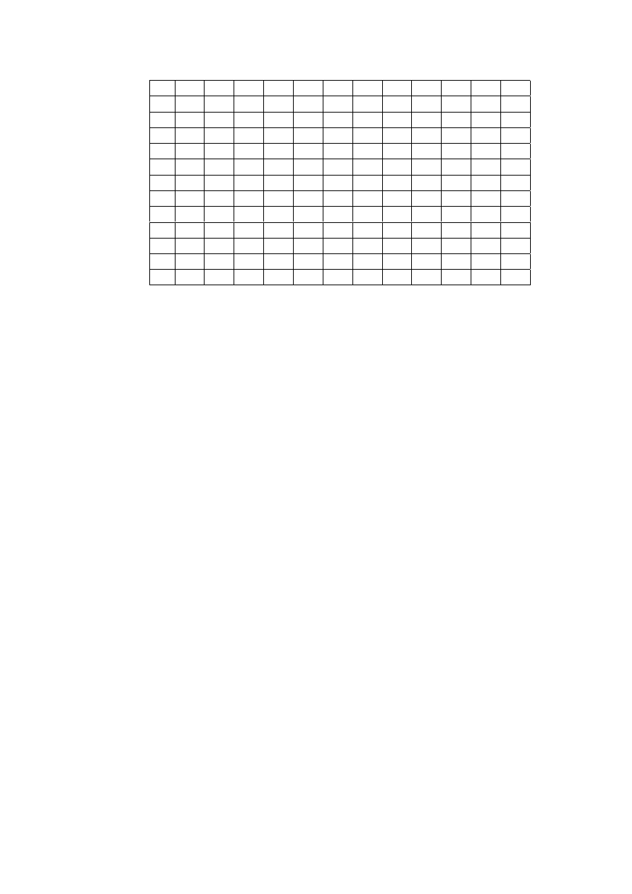
Payoff matrix

In Table 2.2 we have represented the payoffs that are obtained by Player 1 when both
players choose one of the 12 possible strategies.

CHAPTER 2. DECISION ANALYSIS WITH MANY AGENTS

Strategies of Player 1

Strategies of Player 2

1st

scnd move

1st

scnd move

move

if player 2

move

if player 1

has played

move

has played

Table 2.1: List of strategies

2.4.3

Mixed and Behavior Strategies

Mixing strategies

Since a player evaluates outcomes according to his VNM-utility functions he can envi-
sion to “mix” strategies by selecting one of them randomly, according to a lottery that
he will define. This introduces one supplementary chance move in the game descrip-
tion.

For example, if Player

j has p pure strategies γ

, k = 1, . . . , p he can select the

strategy he will play through a lottery which gives a probability

to the pure strategy

k = 1, . . . , p. Now the possible choices of action by Player j are elements of the

set of all the probability distributions

= (x

)

k=1,...,p

≥ 0,

k=1

= 1.

We note that the set

is compact and convex in IR

2.4. GAMES IN NORMAL FORM

-5

-10

-5

-10

Table 2.2: Payoff matrix

Behavior strategies

A behavior strategy is defined as a mapping which associates with the information
available to Player

j at a decision node where he is making a move a probability dis-

tribution over his set of actions.

The difference between mixed and behavior strategies is subtle. In a mixed strat-

egy, the player considers the set of possible strategies and picks one, at random, ac-
cording to a carefully designed lottery. In a behavior strategy the player designs a
strategy that consists in deciding at each decision node, according to a carefully de-
signed lottery, this design being contingent to the information available at this node.
In summary we can say that a behavior strategy is a strategy that includes randomness
at each decision node. A famous theorem [Kuhn, 1953], that we give without proof,
establishes that these two ways of introding randomness in the choice of actions are
equivalent in a large class of games.

Theorem 2.4.1 In an extensive game of perfect recall all mixed strategies can be rep-
resented as behavior strategies.

CHAPTER 2. DECISION ANALYSIS WITH MANY AGENTS

Chapter 3

Solution concepts for noncooperative
games

3.1

introduction

In this chapter we consider games described in their normal form and we propose
different solution concept under the assumption that the players are non cooperating.
In noncooperative games the players do not communicate between each other, they
don’t enter into negotiation for achieving a common course of action. They know that
they are playing a game. They know how the actions, their own and the actions of
the other players, will determine the payoffs of every player. However they will not
cooperate.

To speak of a solution concept for a game one needs, first of all, to describe the

game in its normal form. The solution of an

m-player game will thus be a set of strategy

vectors

γ that have attractive properties expressed in terms of the payoffs received by

the players.

Recall that an

m-person game in normal form is defined by the following data

{M, (Γ

), (V

) for j

∈ M},

where

M is the set of players, M =

{1, 2, ..., m}, and for each player j ∈ M, Γ

is the

set of strategies (also called the strategy space ) and

∈ M, is the payoff function

that assigns a real number

(γ) with a strategy vector γ

∈ Γ

× Γ

× . . . × Γ

In this chapter we shall study different classes of games in normal form. The

first category consists in the so-called matrix games describing a situation where two
players are in a complete antagonistic situation since what a player gains the other

CHAPTER 3. SOLUTION CONCEPTS FOR NONCOOPERATIVE GAMES

player looses, and where each player has a finite choice of strategies. Matrix games
are also called two player zero-sum finite games . The second category will consist
of two player games, again with a finite strategy set for each player, but where the
payoffs are not zero-sum. These are the nonzero-sum matrix games or bimatrix games .
The third category, will be the so-called concave games that encompass the previous
classes of matrix and bimatrix games and for which we will be able to prove nice
existence, uniqueness and stability results for a noncooperative game solution concept
called equilibrium .

3.2

Matrix Games

Definition 3.2.1 A game is zero-sum if the sum of the players’ payoffs is always zero.
Otherwise the game is nonzero-sum. A two-player zero-sum game is also called a duel.

Definition 3.2.2 A two-player zero-sum game in which each player has only a finite
number of actions to choose from is called a matrix game.

Let us explore how matrix games can be “solved”. We number the players 1 and 2
respectively. Conventionally, Player

1 is the maximizer and has m (pure) strategies,

say

i = 1, 2, ..., m, and Player 2 is the minimizer and has n strategies to choose from,

say

j = 1, 2, ..., n. If Player 1 chooses strategy i while Player 2 picks strategy j, then

Player

2 pays Player 1 the amount a

. The set of all possible payoffs that Player

1 can obtain is represented in the form of the m

× n matrix A with entries a

for

i = 1, 2, ..., m and j = 1, 2, ..., n. Now, the element in the i

−th row and j−th column

of the matrix

A corresponds to the amount that Player 2 will pay Player 1 if the latter

chooses strategy

i and the former chooses strategy j. Thus one can say that in the

game under consideration, Player

1 (the maximizer) selects rows of A while Player

2 (the minimizer) selects columns of that matrix, and as the result of the play, Player
2 pays Player 1 the amount of money specified by the element of the matrix in the
selected row and column.

Example 3.2.1 Consider a game defined by the following matrix:

4 10 0

Negative payments are allowed. We could have said also that Player 1 receives the amount

and

Player 2 receives the amount

−a

3.2. MATRIX GAMES

The question now is what can be considered as players’ best strategies.

One possibility is to consider the players’ security levels . It is easy to see that if

Player

1 chooses the first row, then, whatever Player 2 does, Player 1 will get a payoff

equal to at least 1 (util

). By choosing the second row, on the other hand, Player

1 risks

getting 0. Similarly, by choosing the first column Player

2 ensures that he will not have

to pay more than 4, while the choice of the second or third column may cost him 10
or 8, respectively. Thus we say that Player

1’s security level is 1 which is ensured by

the choice of the first row, while Player

2’s security level is 4 and it is ensured by the

choice of the first column. Notice that

1 = max

min

and

4 = min

max

which is the reason why the strategy which ensures that Player

1 will get at least the

payoff equal to his security level is called his maximin strategy . Symmetrically, the
strategy which ensures that Player

2 will not have to pay more than his security level

is called his minimax strategy .

Lemma 3.2.1 The following inequality holds

max

min

≤ min

max

(3.1)

Proof:

The proof of this result is based on the remark that, since both security levels

are achievable, they necessarily satisfy the inequality (3.1). We give below a more
detailed proof.

We note the obvious set of inequalities

min

≤ a

≤ max

(3.2)

which holds for all possible

k and l. More formally, let (i

∗

, j

∗

) and (i

∗

, j

∗

) be defined

∗

= max

min

(3.3)

and

∗

= min

max

(3.4)

A util is the utility unit.

CHAPTER 3. SOLUTION CONCEPTS FOR NONCOOPERATIVE GAMES

respectively. Now consider the payoff

∗

. Then, by (3.2) with

k = i

∗

and

l = j

∗

get

max

(min

)

≤ a

∗

≤ min

(max

QED.

An important observation is that if Player

1 has to move first and Player 2 acts

having seen the move made by Player

1, then the maximin strategy is Player 1’s best

choice which leads to the payoff equal to 1. If the situation is reversed and it is Player
2 who moves first, then his best choice will be the minimax strategy and he will have
to pay 4. Now the question is what happens if the players move simultaneously. The
careful study of the example shows that when the players move simultaneously the
minimax and maximin strategies are not satisfactory “solutions” to this game. Notice
that the players may try to improve their payoffs by anticipating each other’s strategy.
In the result of that we will see a process which in this case will not converge to any
solution.

Consider now another example.

Example 3.2.2 Let the matrix game

A be given as follows






−15

∗

−30 40

−45 60






Can we find satisfactory strategy pairs?

It is easy to see that

max

min

= max

{−15, −30, −45} = −15

and

min

max

= min

{30, −15, 60} = −15

and that the pair of maximin and minimax strategies is given by

(i, j) = (1, 2).

That means that Player

1 should choose the first row while Player 2 should select the

second column, which will lead to the payoff equal to -15.

In the above example, we can see that the players’ maximin and minimax strategies

“solve” the game in the sense that the players will be best off if they use these strategies.

3.2. MATRIX GAMES

3.2.1

Saddle-Points

Let us explore in more depth this class of strategies that solve the zero-sum matrix
game.

Definition 3.2.3 If in a matrix game

A = [a

]

i=1,...,m;j=1,...,n;

there exists a pair

∗

, j

∗

)

such that, for all

i1, . . . , m and j1, . . . , n

∗

≤ a

∗

≤ a

∗

(3.5)

we say that the pair

∗

, j

∗

) is a saddle point in pure strategies for the matrix game.

As an immediate consequence, we see that, at a saddle point of a zero-sum game, the
security levels of the two players are equal, i.e. ,

max

min

= min

max

= a

∗

What is less obvious is the fact that, if the security levels are equal then there exists a
saddle point.

Lemma 3.2.2 If, in a matrix game, the following holds

max

min

= min

max

= v

then the game admits a saddle point in pure strategies.

Proof:

Let

∗

and

∗

be a strategy pair that yields the security level payoffs

v (resp.

−v) for Player 1 (resp. Player 2). We thus have for all i = 1, . . . , m and j = 1, . . . , n

∗

≥ min

∗

= max

min

(3.6)

∗

≤ max

∗

= min

max

(3.7)

Since

max

min

= min

max

= a

∗

= v

by (3.6)-(3.7) we obtain

∗

≤ a

∗

≤ a

∗

which is the saddle point condition.

QED.

Saddle point strategies provide a solution to the game problem even if the players

move simultaneously. Indeed, in Example 3.2.2, if Player

1 expects Player 2 to choose

CHAPTER 3. SOLUTION CONCEPTS FOR NONCOOPERATIVE GAMES

the second column, then the first row will be his optimal choice. On the other hand,
if Player

2 expects Player 1 to choose the first row, then it will be optimal for him

to choose the second column. In other words, neither player can gain anything by
unilaterally deviating from his saddle point strategy. Each strategy constitutes the best
reply the player can have to the strategy choice of his opponent. This observation leads
to the following definition.

Remark 3.2.1 Using strategies

∗

and

∗

, Players

1 and 2 cannot improve their payoff

by unilaterally deviating from

(i)

∗

or (

(j)

∗

) respectively. We call such strategies an

equilibrium.

Saddle point strategies, as shown in Example 3.2.2, lead to both an equilibrium and
a pair of guaranteed payoffs. Therefore such a strategy pair, if it exists, provides a
solution to a matrix game, which is “good” in that rational players are likely to adopt
this strategy pair.

3.2.2

Mixed strategies

We have already indicated in chapter 2 that a player could “mix” his strategies by
resorting to a lottery to decide what to play. A reason to introduce mixed strategies in
a matrix game is to enlarge the set of possible choices. We have noticed that, like in
Example 3.2.1, many matrix games do not possess saddle points in the class of pure
strategies. However Von Neumann proved that saddle point strategy pairs exist in the
class of mixed strategies . Consider the matrix game defined by an

× n matrix A.

(As before, Player

1 has m strategies, Player 2 has n strategies). A mixed strategy for

Player

1 is an m-tuple

x = (x

, x

, ..., x

)

where

are nonnegative for

i = 1, 2, ..., m, and x

+ x

+ ... + x

= 1. Similarly, a

mixed strategy for Player

2 is an n-tuple

y = (y

, y

, ..., y

)

where

are nonnegative for

j = 1, 2, ..., n, and y

+ y

+ ... + y

= 1.

Note that a pure strategy can be considered as a particular mixed strategy with

one coordinate equal to one and all others equal to zero. The set of possible mixed
strategies of Player 1 constitutes a simplex in the space IR

. This is illustrated in

Figure 3.1 for

m = 3. Similarly the set of mixed strategies of Player 2 is a simplex in

. A simplex is, by construction, the smallest closed convex set that contains

n + 1

points in IR

3.2. MATRIX GAMES

Figure 3.1: The simplex of mixed strategies

The interpretation of a mixed strategy, say

x, is that Player 1, chooses his pure

strategy

i with probability x

, i = 1, 2, ..., m. Since the two lotteries defining the

random draws are independent events, the joint probability that the strategy pair

(i, j)

be selected is given by

. Therefore, with each pair of mixed strategies

(x, y) we

can associate an expected payoff given by the quadratic expression (in

x. y)

i=1

j=1

= x

Ay.

The first important result of game theory proved in [Von Neumann 1928] showed

the following

Theorem 3.2.1 Any matrix game has a saddle point in the class of mixed strategies,
i.e. , there exist probability vectors

x and y such that

max

min

Ay = min

max

Ay = (x

∗

)

∗

= v

∗

where

∗

is called the value of the game.

The superscript

denotes the transposition operator on a matrix.

CHAPTER 3. SOLUTION CONCEPTS FOR NONCOOPERATIVE GAMES

We shall not repeat the complex proof given by von Neumann. Instead we shall relate
the search for saddle points with the solution of linear programs. A well known duality
property will give us the saddle point existence result.

3.2.3

Algorithms for the Computation of Saddle-Points

Matrix games can be solved as linear programs. It is easy to show that the following
two relations hold:

∗

= max

min

Ay = max

min

i=1

(3.8)

and

∗

= min

max

Ay = min

max

j=1

(3.9)

These two relations imply that the value of the matrix game can be obtained by solving
any of the following two linear programs:

1. Primal problem

max

subject to

≤

i=1

, j = 1, 2, ..., n

1 =

i=1

≥ 0, i = 1, 2, ...m

2. Dual problem

min

subject to

≥

j=1

, i = 1, 2, ..., m

1 =

j=1

≥ 0, j = 1, 2, ...n

The following theorem relates the two programs together.

Theorem 3.2.2 (Von Neumann [Von Neumann 1928]): Any finite two-person zero-
sum matrix game

A has a value

3.2. MATRIX GAMES

proof:

The value

∗

of the zero-sum matrix game

A is obtained as the common op-

timal value of the following pair of dual linear programming problems. The respective
optimal programs define the saddle-point mixed strategies.

Primal

Dual

max

min

subject to

≥ v1

subject to

A y

≤ z1

1 = 1

y = 1

≥ 0

where

1 =















denotes a vector of appropriate dimension with all components equal to 1. One needs
to solve only one of the programs. The primal and dual solutions give a pair of saddle
point strategies.

•

Remark 3.2.2 Simple

× n games can be solved more easily (see [Owen, 1982]).

Suppose

A is an n

× n matrix game which does not have a saddle point in pure strate-

gies. The players’ unique saddle point mixed strategies and the game value are given
by:

x =

(3.10)

y =

(3.11)

v =

detA

(3.12)

where

is the adjoint matrix of

A, det A the determinant of A, and 1 the vector of

ones as before.

Let us illustrate the usefulness of the above formulae on the following example.

Example 3.2.3 We want to solve the matrix game

−1 2

CHAPTER 3. SOLUTION CONCEPTS FOR NONCOOPERATIVE GAMES

The game, obviously, has no saddle point (in pure strategies). The adjoint

2 0
1 1

and

= [3 1], A

= [2 2], 1A

= 4, det A = 2. Hence the best mixed

strategies for the players are:

x = [

3
4

1
4

y = [

1
2

]

and the value of the play is:

v =

1
2

In other words in the long run Player

1 is supposed to win .5 if he uses the first row

75% of times and the second 25% of times. The Player 2’s best strategy will be to use
the first and the second column

50% of times which ensures him a loss of .5 (only;

using other strategies he is supposed to lose more).

3.3

Bimatrix Games

We shall now extend the theory to the case of a nonzero sum game. A bimatrix game
conveniently represents a two-person nonzero sum game where each player has a finite
set of possible pure strategies.

In a bimatrix game there are two players, say Player

1 and Player 2 who have m and

n pure strategies to choose from respectively. Now, if the players select a pair of pure
strategies, say

(i, j), then Player 1 obtains the payoff a

and Player

2 obtains b

, where

and

are some given numbers. The payoffs for the two players corresponding to

all possible combinations of pure strategies can be represented by two

× n payoff

matrices

A and B with entries a

and

respectively (from here the name).

Notice that a (zero-sum) matrix game is a bimatrix game where

−a

. When

+ b

= 0, the game is a zero-sum matrix game. Otherwise, the game is nonzero-

sum. (As

and

are the players’ payoff this conclusion agrees with Definition

3.2.1.)

Example 3.3.1 Consider the bimatrix game defined by the following matrices

52 44 44
42 46 39

and

50 44 41
42 49 43

3.3. BIMATRIX GAMES

It is often convenient to combine the data contained in two matrices and write it in the
form of one matrix whose entries are ordered pairs

, b

). In this case one obtains

(52, 50)

∗

(44, 44)

(44, 41)

(42, 42)

(46, 49)

∗

(39, 43)

In the above bimatrix some cells have been indicated with asterisks

∗. They correspond

to outcomes resulting from equilibra , a concept that we shall introduce now.

If Player 1 chooses strategy “row 1”, the best reply by Player 2 is to choose strategy

“column 1”, and vice versa. Therefore we say that the outcome (52, 50) is associated
with the equilibrium pair “row 1,column 1”.

The situation is the same for the outcome (46, 49) that is associated with another

equilibrium pair “row 2,column 2”.

We already see on this simple example that a bimatrix game can have many equi-

libria. However there are other examples where no equilibrium can be found in pure
strategies. So, as we have already done with (zero-sum) matrix games, let us expand
the strategy sets to include mixed strategies.

3.3.1

Nash Equilibria

Assume that the players may use mixed strategies . For zero-sum matrix games we have
shown the existence of a saddle point in mixed strategies which exhibits equilibrium
properties. We formulate now the Nash equilibrium concept for the bimatrix games.
The same concept will be defined later on for a more general

m-player case.

Definition 3.3.1 A pair of mixed strategies

∗

, y

∗

) is said to be a Nash equilibrium of

the bimatrix game if

∗

)

A(y

∗

)

≥ x

A(y

∗

) for every mixed strategy x, and

∗

)

B(y

∗

)

≥ (x

∗

)

By for every mixed strategy y.

In an equilibrium, no player can improve his payoff by deviating unilaterally from his
equilibrium strategy.

CHAPTER 3. SOLUTION CONCEPTS FOR NONCOOPERATIVE GAMES

Remark 3.3.1 A Nash equilibrium extends to nonzero sum games the equilibrium
property that was observed for the saddle point solution to a zero sum matrix game.
The big difference with the saddle point concept is that, in a nonzero sum context, the
equilibrium strategy for a player does not guarantee him that he will receive at least the
equilibrium payoff. Indeed if his opponent does not play “well”, i.e. does not use the
equilibrium strategy, the outcome of a player can be anything; there is no guarantee.

Another important step in the development of the theory of games has been the follow-
ing theorem [Nash, 1951]

Theorem 3.3.1 Every finite bimatrix game has at least one Nash equilibrium in mixed
strategies .

Proof:

A more general existence proof including the case of bimatrix games will be

given in the next section.

•

3.3.2

Shortcommings of the Nash equilibrium concept

Multiple equilibria

As noticed in Example 3.3.1 a bimatrix game may have several equilibria in pure strate-
gies. There may be additional equilibria in mixed strategies as well. The nonunique-
ness of Nash equilibria for bimatrix games is a serious theoretical and practical prob-
lem. In Example 3.3.1 one equilibrium strictly dominates the other, ie., gives both
players higher payoffs. Thus, it can be argued that even without any consultations the
players will naturally pick the strategy pair

(i, j) = (1, 1).

It is easy to define examples where the situation is not so clear.

Example 3.3.2 Consider the following bimatrix game

(2, 1)

∗

(0, 0)

(1, 2)

∗

It is easy to see that this game has two equilibria (in pure strategies), none of which
dominates the other. Moreover, Player

1 will obviously prefer the solution (1, 1), while

Player

2 will rather have (2, 2). It is difficult to decide how this game should be played

if the players are to arrive at their decisions independently of one another.

3.3. BIMATRIX GAMES

The prisoner’s dilemma

There is a famous example of a bimatrix game, that is used in many contexts to argue
that the Nash equilibrium solution is not always a “good” solution to a noncooperative
game.

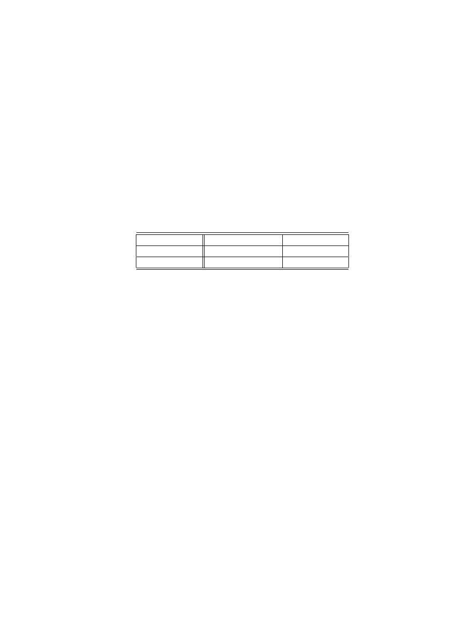
Example 3.3.3 Suppose that two suspects are held on the suspicion of committing
a serious crime. Each of them can be convicted only if the other provides evidence
against him, otherwise he will be convicted as guilty of a lesser charge. By agreeing
to give evidence against the other guy, a suspect can shorten his sentence by half.
Of course, the prisoners are held in separate cells and cannot communicate with each
other. The situation is as described in Table 3.1 with the entries giving the length of the
prison sentence for each suspect, in every possible situation. In this case, the players
are assumed to minimize rather than maximize the outcome of the play. The unique

Suspect I:

Suspect II: refuses

agrees to testify

refuses

(2, 2)

(10, 1)

agrees to testify

(1, 10)

(5, 5)

∗

Table 3.1: The Prisoner’s Dilemma.

Nash equilibrium of this game is given by the pair of pure strategies

(agree

− to −

testif y, agree

− to − testify) with the outcome that both suspects will spend five

years in prison. This outcome is strictly dominated by the strategy pair

(ref use

−to−

testif y, ref use

− to − testify), which however is not an equilibrium and thus is not

a realistic solution of the problem when the players cannot make binding agreements.

This example shows that Nash equilibria could result in outcomes being very far from
efficiency.

3.3.3

Algorithms for the Computation of Nash Equilibria in Bima-
trix Games

Linear programming is closely associated with the characterization and computation
of saddle points in matrix games. For bimatrix games one has to rely to algorithms
solving either quadratic programming or complementarity problems. There are also a
few algorithms (see [Aumann, 1989], [Owen, 1982]) which permit us to find an equi-
librium of simple bimatrix games. We will show one for a

× 2 bimatrix game and

then introduce the quadratic programming [Mangasarian and Stone, 1964] and com-
plementarity problem [Lemke & Howson 1964] formulations.

CHAPTER 3. SOLUTION CONCEPTS FOR NONCOOPERATIVE GAMES

Equilibrium computation in a

× 2 bimatrix game

For a simple

× 2 bimatrix game one can easily find a mixed strategy equilibrium as

shown in the following example.

Example 3.3.4 Consider the game with payoff matrix given below.

(1, 0) (0, 1)

(

1
2

1
3

) (1, 0)

Notice that this game has no pure strategy equilibrium. Let us find a mixed strategy

equilibrium.

Assume Player

2 chooses his equilibrium strategy y (i.e.

100y% of times use

first column,

100(1

− y)% times use second column) in such a way that Player 1 (in

equilibrium) will get as much payoff using first row as using second row i.e.

y + 0(1

− y) =

1
2

y + 1(1

− y).

This is true for

∗

2
3

Symmetrically, assume Player

1 is using a strategy x (i.e. 100x% of times use first

row,

100(1

− y)% times use second row) such that Player 2 will get as much payoff

using first column as using second column i.e.

0x +

1
3

− x) = 1x + 0(1 − x).

This is true for

∗

1
4

. The players’ payoffs will be, respectively,

(

2
3

) and (

1
4

Then the pair of mixed strategies

∗

, 1

− x

∗

), (y

∗

, 1

− y

∗

)

is an equilibrium in mixed strategies.

Links between quadratic programming and Nash equilibria in bimatrix games

Mangasarian and Stone (1964) have proved the following result that links quadratic
programming with the search of equilibria in bimatrix games. Consider a bimatrix

3.3. BIMATRIX GAMES

game

(A, B). We associate with it the quadratic program

max

Ay + x

− v

]

(3.13)

s.t.

≤ v

(3.14)

≤ v

(3.15)

x, y

≥ 0

(3.16)

= 1

(3.17)

= 1

(3.18)

, v

∈ IR.

(3.19)

Lemma 3.3.1 The following two assertions are equivalent

(i)

(x, y, v

, v

) is a solution to the quadratic programming problem (3.13)- (3.19)

(ii)

(x, y) is an equilibrium for the bimatrix game.

Proof:

From the constraints it follows that

≤ v

and

≤ v

for any

feasible

(x, y, v

, v

). Hence the maximum of the program is at most 0. Assume that

(x, y) is an equilibrium for the bimatrix game. Then the quadruple

(x, y, v

= x

Ay, v

= x

By)

is feasible, i.e. satisfies (7.2)-(3.19), and gives to the objective function (7.1) a value
0. Hence the equilibrium defines a solution to the quadratic programming problem
(7.1)-(3.19).

Conversely, let

∗

, y

∗

, v

∗

, v

∗

) be a solution to the quadratic programming problem

(7.1)- (3.19). We know that an equilibrium exists for a bimatrix game (Nash theorem).
We know that this equilibrium is a solution to the quadratic programming problem
(7.1)-(3.19) with optimal value 0. Hence the optimal program

∗

, y

∗

, v

∗

, v

∗

) must also

give a value 0 to the objective function and thus be such that

∗

+ x

∗

= v

∗

+ v

∗

(3.20)

For any

≥ 0 and y ≥ 0 such that x

= 1 and y

= 1 we have, by (3.17) and

(3.18)

∗

≤ v

∗

≤ v

∗

CHAPTER 3. SOLUTION CONCEPTS FOR NONCOOPERATIVE GAMES

In particular we must have

∗

≤ v

∗

≤ v

∗

These two conditions with (3.20) imply

∗

= v

∗

= v

∗

Therefore we can conclude that For any

≥ 0 and y ≥ 0 such that x

= 1 and

= 1 we have, by (3.17) and (3.18)

∗

≤ x

∗

≤ x

∗

and hence,

∗

, y

∗

) is a Nash equilibrium for the bimatrix game.

QED

A Complementarity Problem Formulation

We have seen that the search for equilibria could be done through solving a quadratic
programming problem. Here we show that the solution of a bimatrix game can also be
obtained as the solution of a complementarity problem .

There is no loss in generality if we assume that the payoff matrices are

× n and

have only positive entries (

A > 0 and B > 0). This is not restrictive, since VNM

utilities are defined up to an increasing affine transformation. A strategy for Player 1
is defined as a vector

∈ IR

that satisfies

≥ 0

(3.21)

= 1

(3.22)

and similarly for Player 2

≥ 0

(3.23)

= 1.

(3.24)

It is easily shown that the pair

∗

, y

∗

) satisfying (3.21)-(3.24) is an equilibrium iff

∗

A y

∗

≥ A y

∗

(A > 0)

∗

B y

∗

≥ B

∗

(B > 0)

(3.25)

i.e. if the equilibrium condition is satisfied for pure strategy alternatives only.

3.3. BIMATRIX GAMES

Consider the following set of constraints with

∈ IR and v

∈ IR

≥ A y

∗

≥ B

∗

and

∗

(A y

∗

− v

)

= 0

∗

− v

) = 0

(3.26)

The relations on the right are called complementarity constraints . For mixed strategies
(x

∗

, y

∗

) satisfying (3.21)-(3.24), they simplify to x

∗

A y

∗

= v

∗

B y

∗

= v

. This

shows that the above system (3.26) of constraints is equivalent to the system (3.25).

Define

= x/v

= y/v

and introduce the slack variables

and

, the

system of constraints (3.21)-(3.24) and (3.26) can be rewritten

−

! Ã

(3.27)

0 =

(3.28)

≤

(3.29)

≤

(3.30)

Introducing four obvious new variables permits us to rewrite (3.27)- (3.30) in the
generic formulation

u = q + M s

(3.31)

0 = u

(3.32)

≥ 0

(3.33)

≥ 0,

(3.34)

of a so-called a complementarity problem .

A pivoting algorithm ([Lemke & Howson 1964], [Lemke 1965]) has been proposedto

solve such problems. This algorithm applies also to quadratic programming , so this
confirms that the solution of a bimatrix game is of the same level of difficulty as solving
a quadratic programming problem.

Remark 3.3.2 Once we obtain

x and y, solution to (3.27)-(3.30) we shall have to

reconstruct the strategies through the formulae

x = s

/(s

T
1

)

(3.35)

y = s

/(s

T
2

(3.36)

CHAPTER 3. SOLUTION CONCEPTS FOR NONCOOPERATIVE GAMES

3.4

Concave

m-Person Games

The nonuniqueness of equilibria in bimatrix games and a fortiori in

m-player matrix

games poses a delicate problem. If there are many equilibria, in a situation where
one assumes that the players cannot communicate or enter into preplay negotiations,
how will a given player choose among the different strategies corresponding to the
different equilibrium candidates? In single agent optimization theory we know that
strict concavity of the (maximized) objective function and compactness and convexity
of the constraint set lead to existence and uniqueness of the solution. The following
question thus arises

Can we generalize the mathematical programming approach to a situation
where the optimization criterion is a Nash-Cournot equilibrium? can we
then give sufficient conditions for existence and uniqueness of an equilib-
rium solution?

The answer has been given by Rosen in a seminal paper [Rosen, 1965] dealing with
concave

m-person game .

A concave

m-person game is described in terms of individual strategies repre-

sented by vectors in compact subsets of Euclidian spaces (IR

for Player

j) and by

payoffs represented, for each player, by a continuous functions which is concave w.r.t.
his own strategic variable. This is a generalization of the concept of mixed strategies,
introduced in previous sections. Indeed, in a matrix or a bimatrix game the mixed
strategies of a player are represented as elements of a simplex , i.e. a compact con-
vex set, and the payoffs are bilinear or multilinear forms of the strategies, hence, for
each player the payoff is concave w.r.t. his own strategic variable. This structure is
thus generalized in two ways: (i) the strategies can be vectors constrained to be in a
more general compact convex set and (ii) the payoffs are represented by more general
continuous-concave functions.

Let us thus introduce the following game in strategic form

• Each player j ∈ M = {1, . . . , m} controls the action u

∈ U

a compact convex

subset of IR

, where

is a given integer, and gets a payoff

, . . . , u

where

: U

× . . . × U

, . . .

× U

7→ IR is continuous in each u

and concave

• A coupled constraint is defined as a proper subset U of U

×. . .×U

The constraint is that the joint action

u = (u

, . . . , u

) must be in

3.4. CONCAVE

-PERSON GAMES

Definition 3.4.1 An equilibrium , under the coupled constraint

U is defined as a deci-

sion

m-tuple (u

∗

, . . . , u

∗

, . . . , u

∗

)

∈ U such that for each player j ∈ M

∗

, . . . , u

∗

, . . . , u

∗

)

≥ ψ

∗

, . . . , u

∗

)

(3.37)

for all

∈ U

s.t.

∗

, . . . , u

∗

)

∈ U.

(3.38)

Remark 3.4.1 The consideration of a coupled constraint is a new feature. Now each
player’s strategy space may depend on the strategy of the other players. This may look
awkward in the context of nonocooperative games where thw player cannot enter into
communication or cannot coordinate their actions. However the concept is mathemat-
ically well defined. We shall see later on that it fits very well some interesting aspects
of environmental management. One can think for example of a global emission con-
straint that is imposed on a finite set of firms that are competing on the same market.
This environmental example will be further developed in forthcoming chapters.

3.4.1

Existence of Coupled Equilibria

Definition 3.4.2 A coupled equilibrium is a vector

∗

such that

∗

) = max

{ψ

∗

, . . . , u

∗

)

|(u

∗

, . . . , u

∗

)

∈ U}.

(3.39)

At such a point no player can improve his payoff by a unilateral change in his strategy
which keeps the combined vector in

Let us first show that an equilibrium is actually defined through a fixed point condi-

tion. For that purpose we introduce a so-called global reaction function

θ :

U ×U 7→ IR

defined by

θ(u, v, r) =

j=1

, . . . , v

, . . . , u

(3.40)

where

> 0, j = 1, . . . , m are given weights. The precise role of this weighting

scheme will be explained later. For the moment we could take as well

≡ 1. Notice

that, even if

u and v are in

U, the combined vectors (u

, . . . , v

, . . . , u

) are element

of a larger set in

× . . . × U

. This function is continuous in

u and concave in v

for every fixed

u. We call it a reaction function since the vector v can be interpreted as

composed of the reactions of the different players to the given vector

u. This function

is helpful as shown in the following result.

Lemma 3.4.1 Let

∗

∈ U be such that

θ(u

∗

, u

∗

, r) = max

∈U

θ(u

∗

, u, r).

(3.41)

Then

∗

is a coupled equilibrium.

CHAPTER 3. SOLUTION CONCEPTS FOR NONCOOPERATIVE GAMES

Proof:

Assume

∗

satisfies (3.41) but is not a coupled equilibrium, i.e. does not

satisfy (3.39). Then, for one player, say

`, there would exist a vector

u = (u

∗

, . . . , u

∗

)

∈ U

such that

∗

, . . . , u

∗

) > ψ

∗

Then we shall also have

θ(u

∗

, ¯

u) > θ(u

∗

, u

∗

) which is a contradiction to (3.41). QED

This result has two important consequences.

1. It shows that proving the existence of an equilibrium reduces to proving that a

fixed point exists for an appropriately defined reaction mapping (

∗

is the best

reply to

∗

in (3.41));

2. it associates with an equilibrium an implicit maximization problem , defined in

(3.41). We say that this problem is implicit since it is defined in terms of its
solution

∗

To make more precise the fixed point argument we introduce a coupled reaction map-
ping .

Definition 3.4.3 The point to set mapping

Γ(u, r) =

{v|θ(u, v, r) = max

∈U

θ(u, w, r)

(3.42)

is called the coupled reaction mapping associated with the positive weighting

r. A

fixed point of

Γ(

·, r) is a vector u

∗

such that

∗

∈ Γ(u

∗

, r).

By Lemma 3.4.1 a fixed point of

Γ(

·, r) is a coupled equilibrium.

Theorem 3.4.1 For any positive weighting

r there exists a fixed point of Γ(

·, r), i.e. a

point

∗

s.t.

∗

∈ Γ(u

∗

, r). Hence a coupled equilibrium exists.

Proof:

The proof is based on the Kakutani fixed-point theorem that is given in the

Appendix of section 3.8. One is required to show that the point to set mapping is upper
semicontinuous.

QED

Remark 3.4.2 This existence theorem is very close, in spirit, to the theorem of Nash.
It uses a fixed-point result which is “topological” and not “constructive”, i.e. it does
not provide a computational method. However, the definition of a normalised equilib-
rium introduced by Rosen establishes a link between mathematical programming and
concave games with coupled constraints.

3.4. CONCAVE

-PERSON GAMES

3.4.2

Normalized Equilibria

Kuhn-Tucker multipliers

Suppose that the coupled constraint (3.39) can be defined by a set of inequalities

(u)

≥ 0, k = 1, . . . , p

(3.43)

where

: U

× . . . × U

→ IR, k = 1, . . . , p, are given concave functions. Let

us further assume that the payoff functions

(

·) as well as the constraint functions

(

·) are continuously differentiable and satisfy the constraint qualification conditions

so that Kuhn-Tucker multipliers exist for each of the implicit single agent optimization
problems defined below.

Assume all players other than Player

j use their strategy u

∗

∈ M, i 6= j. Then the

equilibrium conditions (3.37)-(3.39) define a single agent optimization problem with
concave objective function and convex compact admissible set. Under the assumed
constraint qualification assumption there exists a vector of Kuhn-Tucker multipliers
λ

= (λ

)

k=1,...,p

such that the Lagrangean

([u

∗−j

, u

], λ

) = ψ

([u

∗−j

, u

]) +

k=1...p

([u

∗−j

, u

])

(3.44)

verifies, at the optimum

0 =

∂

∂u

([u

∗−j

, u

∗

], λ

)

(3.45)

≤ λ

(3.46)

0 = λ

([u

∗−j

, u

∗

])

k = 1, . . . , p.

(3.47)

Definition 3.4.4 We say that the equilibrium is normalized if the different multipliers
λ

for

∈ M are colinear with a common vector λ

, namely

(3.48)

where

> 0 is a given weighting of the players.

Actually, this common multiplier

is associated with the implicit mathematical pro-

gramming problem

max

∈U

θ(u

∗

, u, r)

(3.49)

to which we associate the Lagrangean

(u, λ

) =

∈M

([u

∗−j

, u

]) +

k=1...p

(u).

(3.50)

CHAPTER 3. SOLUTION CONCEPTS FOR NONCOOPERATIVE GAMES

and the first order necessary conditions

0 =

∂

∂u

∗

) +

k=1,...,p

∗

)

}, j ∈ M

(3.51)

≤ λ

(3.52)

0 = λ

∗

)

k = 1, . . . , p.

(3.53)

An economic interpretation

The multiplier, in a mathematical programming framework, can be interpreted as a
marginal cost associated with the right-hand side of the constraint. More precisely it
indicates the sensitivity of the optimum solution to marginal changes in this right-hand-
side. The multiplier permits also a price decentralization in the sense that, through an
ad-hoc pricing mechanism the optimizing agent is induced to satisfy the constraints. In
a normalized equilibrium, the shadow cost interpretation is not so apparent; however,
the price decomposition principle is still valid. Once the common multiplier has been
defined, with the associated weighting

> 0, j = 1, . . . , m the coupled constraint will

be satisfied by equilibrium seeking players, when they use as payoffs the Lagrangeans

([u

∗−j

, u

], λ

) = ψ

([u

∗−j

, u

]) +

k=1...p

([u

∗−j

, u

]),

j = 1, . . . , m.

(3.54)

The common multiplier permits then an “implicit pricing” of the common constraint
so that it remains compatible with the equilibrium structure. Indeed, this result to be
useful necessitates uniqueness of the normalized equilibrium associated with a given
weighting

> 0, j = 1, . . . , m. In a mathematical programming framework, unique-

ness of an optimum results from strict concavity of the objective function to be max-
imized. In a game structure, uniqueness of the equilibrium will result from a more
stringent strict concavity requirement, called by Rosen strict diagonal concavity .

3.4.3

Uniqueness of Equilibrium

Let us consider the so-called pseudo-gradient defined as the vector

g(u, r) =








∂

∂u

(u)

∂

∂u

(u)

∂

∂u

(u)








(3.55)

3.4. CONCAVE

-PERSON GAMES

We notice that this expression is composed of the partial gradients of the different
payoffs with respect to the decision variables of the corresponding player. We also
consider the function

σ(u, r) =

j=1

(u)

(3.56)

Definition 3.4.5 The function

σ(u, r) is diagonally strictly concave on

U if, for every

U, the following holds

− u

)

g(u

, r) + (u

− u

)

g(u

, r) > 0.

(3.57)

A sufficient condition that

σ(u, r) be diagonally strictly concave is that the symmetric

matrix

[G(u, r) + G(u, r)

] be negative definite for any u

U, where G(u, r) is the

Jacobian of

g(u

, r) with respect to u.

Theorem 3.4.2 If

σ(u, r) is diagonally strictly concave on the convex set

U, with the

assumptions insuring existence of K.T. multipliers, then for every

r > 0 there exists a

unique normalized equilibrium

Proof

We sketch below the proof given by Rosen [Rosen, 1965]. Assume that for

some

r > 0 we have two equilibria u

and

. Then we must have

h(u

)

≥ 0

(3.58)

h(u

)

≥ 0

(3.59)

and there exist multipliers

≥ 0, λ

≥ 0, such that

h(u

) = 0

(3.60)

h(u

) = 0

(3.61)

and for which the following holds true for each player

∈ M

∇

) + λ

∇

h(u

) = 0

(3.62)

∇

) + λ

∇

h(u

) = 0.

(3.63)

We multiply (3.62) by

− u

)

and (3.63) by

− u

)

and we sum together

to obtain an expression

β + γ = 0, where, due to the concavity of the h

and the

conditions (3.58)-(3.61)

γ =

∈M

k=1

{λ

1
k

− u

)

∇

) + λ

2
k

− u

)

∇

)

}

≥

∈M

{λ

[h(u

)

− h(u

)] + λ

[h(u

)

− h(u

)]

}

∈M

{λ

h(u

) + λ

h(u

)

} ≥ 0,

(3.64)

CHAPTER 3. SOLUTION CONCEPTS FOR NONCOOPERATIVE GAMES

and

β =

∈M

[(u

− u

)

∇

) + (u

− u

)

∇

)].

(3.65)

Since

σ(u, r) is diagonally strictly concave we have β > 0 which contradicts β+γ = 0.

QED

3.4.4

A numerical technique

The diagonal strict concavity property that yielded the uniqueness result of theorem 3.4.2
also provides an interesting extension of the gradient method for the computation of
the equilibrium. The basic idea is to ”project”, at each step, the pseudo gradient

g(u, r)

on the constraint set

U = {u : h(u) ≥ 0} (let’s call ¯g(u

, r) this projection) and to

proceed through the usual steepest ascent step

`+1

= u

+ τ

g(u

, r).

Rosen shows that, at each step

` the step size τ

> 0 can be chosen small enough for

having a reduction of the norm of the projected gradient. This yields convergence of
the procedure toward the unique equilibrium.

3.4.5

A variational inequality formulation

Theorem 3.4.3 Under assumptions 3.5.1 the vector

∗

= (q

∗

, . . . , q

∗

) is a Nash-

Cournot equilibrium if and only if it satisfies the following variational inequality

− q

∗

)

g(q

∗

)

≤ 0,

(3.66)

where

g(q

∗

) is the pseudo-gradient at q

∗

with weighting

Proof:

Apply first order necessary and sufficient optimality conditions for each player

and aggregate to obtain (3.66).

QED

Remark 3.4.3 The diagonal strict concavity assumption is then equivalent to the prop-
erty of strong monotonicity of the operator

g(q

∗

) in the parlance of variational in-

equality theory.

3.5. COURNOT EQUILIBRIUM

3.5

Cournot equilibrium

The model proposed in 1838 by [Cournot, 1838] is still one of the most frequently used
game model in economic theory. It represents the competition between different firms
supplying a market for a divisible good.

3.5.1

The static Cournot model

Let us first of all recall the basic Cournot oligopoly model. We consider a single
market on which

m firms are competing. The market is characterized by its (inverse)

demand law

p = D(Q) where p is the market clearing price and Q =

j=1,...,m

the total supply of goods on the market. The firm

j faces a cost of production C

hence, letting

q = (q

, . . . , q

) represent the production decision vector of the m firms

together, the profit of firm

j is π

(q) = q

D(Q)

− C

). The following assumptions

are placed on the model

Assumption 3.5.1 The market demand and the firms cost functions satisfy the follow-
ing (i) The inverse demand function is finite valued, nonnegative and defined for all
Q

∈ [0, ∞). It is also twice differentiable, with D

(Q) < 0 wherever D(Q) > 0.

In addition

D(0) > 0. (ii) C

) is defined for all q

∈ [0, ∞), nonnegative, convex,

twice continuously differentiable, and

) > 0. (iii) Q D(Q) is bounded and strictly

concave for all

Q such that D(Q) > 0.

If one assumes that each firm

j chooses a supply level q

∈ [0, ¯q

], this model satis-

fies the definition of a concave game `a la Rosen (see exercise 3.7). There exists an
equilibrium. Let us consider the uniqueness issue in the duopoly case.

Consider the pseudo gradient (there is no need of weighting

, r

) since the con-

straints are not coupled)

g(q

, q

) =

D(Q) + q

(Q)

− C

)

D(Q) + q

(Q)

− C

)

and the jacobian matrix

G(q

, q

) =

(Q) + q

(Q)

− C

)

(Q) + q

(Q)

(Q) + q

(Q)

(Q) + q

(Q)

− C

)

The negative definiteness of the symmetric matrix

1
2

[G(q

, q

) + G(q

, q

)

] =

(Q) + q

(Q)

− C

)

(Q) +

1
2

Q D

(Q)

(Q) +

1
2

Q D

(Q)

(Q) + q

(Q)

− C

)

CHAPTER 3. SOLUTION CONCEPTS FOR NONCOOPERATIVE GAMES

implies uniqueness of the equilibrium.

3.5.2

Formulation of a Cournot equilibrium as a nonlinear com-
plementarity problem

We have seen, when we dealt with Nash equilibria in

m-matrix games, that a solution

could be found through the solution of a linear complementarity problem. A similar
formulation holds for a Cournot equilibrium and it will in general lead to a nonlinear
complementarity problem or NLCP, a class of problems that has recently been the
object of considerable developments in the field of Mathematical Programming (see
e.g. the book [Ferris & Pang, 1997a] and the survey paper [Ferris & Pang, 1997b]) We
can rewrite the equilibrium condition as an NLCP in canonical form

≥ 0

(3.67)

(q)

≥ 0

(3.68)

(q) = 0,

(3.69)

where

(q) =

−D(Q) − q

(Q) + C

(3.70)

The relations (3.67-3.69) express that, at a Cournot equilibrium, either

= 0 and the

gradient

(q) is

≤ 0, or q

> 0 and g

(q) = 0. There are now optimization softwares

that solve these types of problems. In [Rutherford, 1995] an extension of the GAMS
(see [Brooke et al., 1992]) modeling software to provide an ability to solve this type of
complementarity problem is described. More recently the modeling language AMPL
(see [Fourer et al., 1993]) has also been adapted to handel a problem of this type and
to submit it to an efficient NLCP solver like PATH (see [Ferris & Munson, 1994]).

Example 3.5.1 This example comes from the AMPL website

http://www.ampl.com/ampl/TRYAMPL/

Consider an oligopoly with

n = 10 firms. The production cost function of firm j is

given by

) = c

1 + β

)

(1+β

)/β

(3.71)

The market demand function is defined by

D(Q) = (A/Q)

1/γ

(3.72)

Therefore

(Q) =

(A/Q)

1/γ

−1

(

−

) =

−

D(Q)/Q.

(3.73)

3.5. COURNOT EQUILIBRIUM

The Nash Cournot equilibrium will be the solution of the NLCP (3.67-3.69) where

(q) =

−D(Q) − q

(Q) + C

)

−(A/Q)

1/γ

D(Q)/Q + c

+ (L

)

1/β

AMPL input

%%%%%%%FILE nash.mod%%%%%%%%%%

#==>nash.gms

# A non-cooperative game example: a Nash equilibrium is sought.

# References:

# F.H. Murphy, H.D. Sherali, and A.L. Soyster, "A Mathematical

Programming Approach for Determining Oligopolistic Market

Equilibrium", Mathematical Programming 24 (1986), pp. 92-

106.

# P.T. Harker, "Accelerating the convergence . . .", Mathematical

Programming 41 (1988), pp. 29-59.

set Rn := 1 .. 10;

param gamma := 1.2;

param c {i in Rn};

param beta {i in Rn};

param L {i in Rn} := 10;

var q {i in Rn} >= 0;

# production vector

var Q = sum {i in Rn} q[i];

var divQ = (5000/Q)**(1/gamma);

s.t. feas {i in Rn}:

q[i] >= 0 complements

0 <= c[i] + (L[i] * q[i])**(1/beta[i]) - divQ

- q[i] * (-1/gamma) * divQ / Q;

%%%%%%%FILE nash.dat%%%%%%%%%%

data;

param c :=

CHAPTER 3. SOLUTION CONCEPTS FOR NONCOOPERATIVE GAMES

1 5

2 3

3 8

4 5

5 1

6 3

7 7

8 4

9 6

10 3

;

param beta :=

1 1.2

2 1

3 .9

4 .6

5 1.5

6 1

7 .7

8 1.1

9 .95

10 .75

;

%%%%%%%FILE nash.run%%%%%%%%%%

model nash.mod;

data nash.dat;

set initpoint := 1 .. 4;

param initval {Rn,initpoint} >= 0;

data;param initval

: 1 2 3 4 :=

1 1

10 1.0 7

2 1

10 1.2 4

3 1

10 1.4 3

4 1

10 1.6 1

5 1

10 1.8 18

6 1

10 2.1 4

7 1

10 2.3 1

8 1

10 2.5 6

9 1

10 2.7 3

10 1

10 2.9 2

;

for {point in initpoint}

3.6. CORRELATED EQUILIBRIA

{

let{i in Rn} q[i] := initval[i,point];

solve;

include compchk

}

3.5.3

Computing the solution of a classical Cournot model

There are many approaches to find a solution to a static Cournot game. We have
described above the one based on a solution of an NLCP. We list below a few other
alternatives

(a) one discretizes the decision space and uses the complementarity algorithm pro-

posed in [Lemke & Howson 1964] to compute a solution to the associated bima-
trix game;

(b) one exploits the fact that the players are uniquely coupled through the condi-

tion that

Q =

j=1,...,m

and a sort of primal-dual search technique is used

[Murphy,Sherali & Soyster, 1982];

(c) one formulates the Nash-Cournot equilibrium problem as a variational inequal-

ity. Assumption 3.5.1 implies Strict Diagonal Concavity (SDC) , in the sense of
Rosen, i.e. strict monotonicity of the pseudo-gradient operator, hence unique-
ness and convergence of various gradient like algorithms.

3.6

Correlated equilibria

Aumann, [Aumann, 1974], has proposed a mechanism that permits the players to enter
into preplay arrangements so that their strategy choices could be correlated, instead
of being independently chosen, while keeping an equilibrium property. He called this
type of solution correlated equilibrium.

CHAPTER 3. SOLUTION CONCEPTS FOR NONCOOPERATIVE GAMES

3.6.1

Example of a game with correlated equlibria

Example 3.6.1 This example has been initially proposed by Aumann [Aumann, 1974].
Consider a simple bimatrix game defined as follows

5, 1 0, 0

4, 4 1, 5

This game has two pure strategy equilibria

, c

) and (r

, c

) and a mixed strategy

equilibrium where each player puts the same probality 0.5 on each possible pure strat-
egy. The respective outcomes are shown in Table 3.2 Now, if the players agree to play

, c

)

5,1

, c

)

1,5

(0.5

− 0.5, 0.5 − 0.5) : 2.5,2.5

Table 3.2: Outcomes of the three equilibria

by jointly observing a “coin flip” and playing

, c

) if the result is “head”, (r

, c

) if

it is “tail” then they expect the outcome

3, 3 which is a convex combination of the two

pure equilibrium outcomes.

By deciding to have a coin flip deciding on the equilibrium to play, a new type of

equilibrium has been introduced that yields an outcome located in the convex hull of
the set of Nash equilibrium outcomes of the bimatrix game. In Figure 3.2 we have
represented these different outcomes. The three full circles represent the three Nash
equilibrium outcomes. The triangle defined by these three points is the convex hull of
the Nash equilibrium outcomes. The empty circle represents the outcome obtained by
agreeing to play according to the coin flip mechanism.

(3,3)

(2.5,2.5)

(1,5)

(5,1)

Figure 3.2: The convex hull of Nash equilibria

3.6. CORRELATED EQUILIBRIA

It is easy to see that this way to play the game defines an equilibrium for the exten-

sive game shown in Figure 3.3. This is an expanded version of the initial game where,
in a preliminary stage, “Nature” decides randomly the signal that will be observed by
the players

. The result of the ”coin flip” is a “public information”, in the sense that

AUt

Head

Tail

PPP

(5,1)

(0,0)

(4,4)

(1,5)

(5,1)

(0,0)

(4,4)

(1,5)

0.5

Figure 3.3: Extensive game formulation with “Nature” playing first

it is shared by all the players. One can easily check that the correlated equilibrium is
a Nash equilibrium for the expanded game.

We now push the example one step further by assuming that the players agree to

play according to the following mechanism: A random device selects one cell in the
game matrix with the probabilities shown in Figure 3.74.

1
3

(3.74)

When a cell is selected, then each player is told to play the corresponding pure strategy.
The trick is that a player is told what to play but is not told what the recommendation to
the other player is. The information received by each player is not “public” anymore.
More precisely, the three possible signals are

, c

), (r

, c

), (r

, c

). When Player 1

Dotted lines represent information sets of Player 2.

CHAPTER 3. SOLUTION CONCEPTS FOR NONCOOPERATIVE GAMES

receives the signal “play

” he knows that with a probability

1
2

the other player has

been told “play

” and with a probability

1
2

the other player has been told “play

”. When player 1 receives the signal “play

” he knows that with a probability

the other player has been told “play

”. Consider now what Player 1 can do, if he

assumes that the other player plays according to the recommendation. If Player 1 has
been told “play

” and if he plays so he expects

1
2

× 4 +

1
2

× 1 = 2.5;

if he plays

instead he expects

1
2

× 5 +

1
2

× 0 = 2.5

so he cannot improve his expected reward. If Player 1 has been told “play

” and

if he plays so he expects

5, whereas if he plays r

he expects

4. So, for Player 1,

obeying to the recommendation is the best reply to Player 2 behavior when he himself
plays according to the suggestion of the signalling scheme. Now we can repeat the the
verification for Player 2. If he has been told “play

” he expects

1
2

× 1 +

1
2

× 4 = 2.5;

if he plays

instead he expects

1
2

× 0 +

1
2

× 5 = 2.5

so he cannot improve. If he has been told “play

” he expects

5 whereas if he plays

instead he expects

4 so he is better off with the suggested play. So we have checked

that an equilibrium property holds for this way of playing the game. All in all, each
player expects

1
3

× 5 +

1
3

× 1 +

1
3

× 4 = 3 +

1
3

from a game played in this way. This is illustrated in Figure 3.4 where the black spade
shows the expected outcome of this mode of play. Auman called it a ”correlated equi-
librium”. Indeed we can now mix these equilibria and still keep the correlated equi-
librium property, as indicated by the doted line on Figure 3.4; also we can construct
an expanded game in extensive form for which the correlated equilibrium constructed
as above defines a Nash equilibrium (see Exercise 3.6).

In the above example we have seen that, by expanding the game via the adjunction of
a first stage where “Nature” plays and gives information to the players, a new class
of equilibria can be reached that dominate, in the outcome space, some of the original
Nash-equilibria. If the random device gives an information which is common to all
players, then it permits a mixing of the different pure strategy Nash equilibria and the
outcome is in the convex hull of the Nash equilibrium outcomes. If the random device
gives an information which may be different from one player to the other, then the
correlated equilibrium can have an outcome which lies out of the convex hull of Nash
equilibrium outcomes.

3.6. CORRELATED EQUILIBRIA

(3,3)

(2.5,2.5)

(1,5)

(5,1)

(3.33,3.33)

♠

··

···

Figure 3.4: The dominating correlated equilibrium

3.6.2

A general definition of correlated equilibria

Let us give a general definition of a correlated equilibrium in an

m-player normal form

game. We shall actually give two definitions. The first one describes the construct
of an expanded game with a random device distributing some pre-play information to
the players. The second definition which is valid for

m-matrix games is much simpler

although equivalent.

Nash equilibrium in an expanded game

Assume that a game is described in normal form, with

m players j = 1, . . . , m, their

respective strategy sets

and payoffs

(γ

, . . . , γ

). This will be called the

original normal form game.

Assume the players may enter into a phase of pre-play communication during

which they design a correlation device that will provide randomly a signal called pro-
posed mode of play. Let

E =

{1, 2, . . . , L} be the finite set of the possible modes of

play. The correlation device will propose with probability

λ(`) the mode of play `.

The device will then give the different players some information about the proposed
mode of play. More precisely, let

be a class of subsets of

E, called the information

structure of player

j. Player j, when the mode of play ` has been selected, receives an

information denoted

(`)

∈ H

. Now, we associate with each player

j a meta strategy

denoted

: H

→ Γ

that determines a strategy for the original normal form game,

on the basis of the information received. All this construct, is summarized by the data
(E,

{λ(`)}

∈E

(`)

∈ H

}

∈M,`∈E

{˜γ

∗

: H

→ Γ

}

∈M

) that defines an expanded

game.

Definition 3.6.1 The data

(E,

{λ(`)}

∈E

(`)

∈ H

}

∈M,`∈E

{˜γ

∗

: H

→ Γ

}

∈M

)

CHAPTER 3. SOLUTION CONCEPTS FOR NONCOOPERATIVE GAMES

defines a correlated equilibrium of the original normal form game if it is a Nash equi-
librium for the expanded game i.e. if no player can improve his expected payoff by
changing unilaterally his meta strategy, i.e. by playing

(`)) instead of ˜

∗

(`))

when he receives the signal

(`)

∈ H

∈E

λ(`)V

([˜

∗

(`)), ˜

∗

−j

(`))]

≥

∈E

λ(`)V

([˜

(`)), ˜

∗

−j

(`))].

(3.75)

An equivalent definition for

m-matrix games

In the case of an

m-matrix game, the definition given above can be replaced with the

following one, which is much simpler

Definition 3.6.2 A correlated equilibrium is a probability distribution

π(s) over the

set of pure strategies

S = S

× S

. . .

× S

such that, for every player

j and any

mapping

: S

→ S

the following holds

∈S

π(s)V

([s

, s

−j

])

≥

∈S

π(s)V

([δ(s

), s

−j

]).

(3.76)

3.7

Bayesian equilibrium with incomplete information

Up to now we have considered only games where each player knows everything con-
cerning the rules, the players types (i.e. their payoff functions, their strategy sets) etc...
We were dealing with games of complete information. In this section we look at a
particular class of games with incomplete information and we explore the class of so-
called Bayesian equilibria.

3.7.1

Example of a game with unknown type for a player

In a game of incomplete information, some players do not know exactly what are the
characteristics of other players. For example, in a two-player game, Player 2 may not
know exactly what the payoff function of Player 1 is.

Example 3.7.1 Consider the case where Player 1 could be of two types, called

and

respectively. We define below two matrix games, corresponding to the two possible

3.7. BAYESIAN EQUILIBRIUM WITH INCOMPLETE INFORMATION

types respectively:

−1 2, 0

2, 1

3, 0

1.5,

−1 3.5, 0

2, 1

3, 0

Game 1

Game 2

If Player 1 is of type

, then the bimatrix game 1 is played; if Player 1 is of type

then the bimatrix game 2 is played; the problem is that Player 2 does not know the type
of Player 1.

3.7.2

Reformulation as a game with imperfect information

Harsanyi, in [Harsanyi, 1967-68], has proposed a transformation of a game of incom-
plete information into a game with imperfect information. For the example 3.7.1 this
transformation introduces a preliminary chance move, played by Nature which decides
randomly the type

of Player 1. The probability distribution of each type, denoted

and

respectively, represents the beliefs of Player 2, given here in terms of prior

probabilities, about facing a player of type

. One assumes that Player 1 knows

also these beliefs, the prior probabilities are thus common knowledge. The information
structure

in the associated extensive game shown in Figure 3.5, indicates that Player 1

knows his type when deciding, whereas Player 2 does not observe the type neither,
indeed in that game of simultaneous moves, the action chosen by Player 1. Call

(resp.

−x

) the probability of choosing

(resp.

) by Player 1 when he implements

a mixed strategy, knowing that he is of type

. Call

y (resp. 1

− y) the probability of

choosing

(resp.

) by Player 2 when he implements a mixed strategy.

We can define the optimal response of Player 1 to the mixed strategy

(y, 1

− y) of

Player 2 by solving

max

i=1,2

y + a

− y)

if the type is

max

i=1,2

y + a

− y)

if the type is

We can define the optimal response of Player 2 to the pair of mixed strategy

, 1

−

), i = 1, 2 of Player 1 by solving

max

j=1,2

+ (1

− x

) + p

+ (1

− x

The dotted line in Figure 3.5 represents the information set of Player 2.

We call

and

the payoffs of Player 1 and Player 2 respectively when the type is

CHAPTER 3. SOLUTION CONCEPTS FOR NONCOOPERATIVE GAMES

AUt

PPP

(0,-1)

(2,0)

(2,1)

(3,0)

(1.5,-1)

(3.5,0)

(2,1)

(3,0)

Figure 3.5: Extensive game formulation of the game of incomplete information

Let us rewrite these conditions with the data of the game illustrated in Figure 3.5. First
consider the reaction function of Player 1

⇒ max{0y + 2(1 − y), 2y + 3(1 − y)}

⇒ max{1.5y + 3.5(1 − y), 2y + 3(1 − y)}.

We draw in Figure 3.6 the lines corresponding to these comparisons between two linear
functions. We observe that, if Player 1’s type is

, he will always choose

, whatever

y, whereas, if his type is θ

he will choose

y is mall enough and switch to r

when

y > 0.5. For y = 0.5, the best reply of Player 1 could be any mixed strategy (x, 1

− x).

Consider now the optimal reply of Player 2. We know that Player 1, if he is of type

xhooses always action

i.e.

= 0. So the best reply conditions for Player 2 can

be written as follows

max

{(p

(

−1)+(1−p

)(x

(

−1)+(1−x

)1)), (p

(0) + (1

−p

)(x

(0) + (1

−x

)0))

}

which boils down to

max

{(1 − 2(1 − p

)x), 0)

We conclude that Player 2 chooses action

2(1

−p

)

, action

2(1

−p

)

and any mixed action with

∈ [0, 1] if x

2(1

−p

)

. We conclude easily from these

observations that the equilibria of this game are characterized as follows:

3.7. BAYESIAN EQUILIBRIUM WITH INCOMPLETE INFORMATION

XXXXX

p p p p p p p p p p p p p p p p p p p p

XXXXX

p p p p p p p p p p p p p p p p p p p p

0.5

3.5

1.5

Figure 3.6: Optimal reaction of Player 1 to Player 2 mixed strategy

(y, 1

− y)

≡ 0

≤ 0.5 x

= 0, y = 1 or x

= 1, y = 0 or x

2(1

−p

)

, y = 0.5

> 0.5

= 0, y = 1.

3.7.3

A general definition of Bayesian equilibria

We can generalize the analysis performed on the previous example and introduce the
following definitions. Let

M be a set of m players. Each player j

∈ M may be of

different possible types. Let

be the finite set of types for Player

j. Whatever his

type, Payer

j has the same set of pure strategies

. If

θ = (θ

, . . . .θ

)

∈ Θ =

× . . . × Θ

is a type specification for every player, then the normal form of the

game is specified by the payoff functions

(θ;

·, . . . , ·) : S

× . . . × S

→ IR, j ∈ M.

(3.77)

A prior probability distribution

p(θ

, . . . .θ

) on Θ is given as common knowledge. We

assume that all the marginal probabilities are nonzero

(θ

) > 0,

∀j ∈ M.

When Player

j observes that he is of type θ

∈ Θ

he can construct his revised condi-

tional probality distribution on the types

−j

of the other players through the Bayes

formula

p(θ

−j

|θ

) =

p([θ

, θ

−j

])

(θ

)

(3.78)

We can now introduce an expanded game where Nature draws randomly, according to
the prior probability distribution

·), a type vector θ ∈ Θ for all players. Player-j can

observe only his own type

∈ Θ

. Then each player

∈ M picks a strategy in his

own strategy set

. The outcome is then defined by the payoff functions (3.77).

CHAPTER 3. SOLUTION CONCEPTS FOR NONCOOPERATIVE GAMES

Definition 3.7.1 In a game of incomplete information with

m players having respec-

tive type sets

and pure strategy sets

i = 1, . . . , m, a Bayesian equilibrium is a

Nash equilibrium in the “ expanded game ” in which each player pure strategy

is a

map from

The expanded game can be described in its normal form as follows. Each player

∈ M

has a strategy set

where a strategy is defined as a mapping

: Θ

→ S

. Associated

with a strategy profile

γ = (γ

, . . . , γ

) the payoff to player j is given by

(γ) =

∈Θ

(θ

)

−j

∈Θ

−j

p(θ

−j

|θ

)

([θ

, θ

−j

]; γ

(θ

), . . . , γ

(θ

), . . . , γ

(θ

)).

(3.79)

As usual, a Nash equilibrium is a strategy profile

∗

= (γ

∗

, . . . , γ

∗

)

∈ Γ = Γ

× . . . ×

such that

(γ

∗

)

≥ V

(γ

, γ

∗

−j

)

∀γ

∈ Γ

(3.80)

It is easy to see that, since each

(θ

) is positive, the equilibrium conditions (3.80)

lead to the following conditions

∗

(θ

) = argmax

∈S

−j

∈Θ

−j

p(θ

−j

|θ

) u

([θ

, θ

−j

]; [s

, γ

∗

−j

(θ

−j

)])

∈ M.(3.81)

Remark 3.7.1 Since the sets

and

are finite, the set

of mappings from

is also finite. Therefore the expanded game is an

m-matrix game and, by Nash theorem

there exists at least one mixed strategy equilibrium.

3.8

Appendix on Kakutani Fixed-point theorem

Definition 3.8.1 Let

Φ : IR

7→ 2IR

be a point to set mapping. We say that this

mapping is upper semicontinuous if, whenever the sequence

}

k=1,2,...

converges in

toward

then any accumulation point

of the sequence

}

k=1,2,...

in IR

, where

∈ Φ(x

), k = 1, 2, . . ., is such that y

∈ Φ(x

Theorem 3.8.1 Let

Φ : A

7→ 2

be a point to set upper semicontinuous mapping,

where

A is a compact subset

of IR

. Then there exists a fixed-point for

Φ. That is,

there is

∗

∈ Φ(x

∗

) for some x

∗

∈ A.

i.e. a closed and bounded subset.

3.9. EXERCISES

3.9

exercises

Exercise 3.1:

Consider the matrix game.

4 10 0

Assume that the players are in the simultaneous move information structure. Assume
that the players try to guess and counterguess the optimal behavior of the opponent in
order to determine their optimal strategy choice. Show that this leads to an unstable
process.

Exercise 3.2:

Find the value and the saddle point mixed-strategies for the above ma-

trix game.

Exercise 3.3:

Define the quadratic programming problem that will find a Nash equi-

librium for the bimatrix game

(52, 50)

∗

(44, 44)

(44, 41)

(42, 42)

(46, 49)

∗

(39, 43)

Verify that the entries marked with a

∗ correspond to a solution of the associated

quadratic programming problem.

Exercise 3.4:

Do the same as above but using now the complementarity problem

formulation.

Exercise 3.5:

Consider the two player game where the strategy sets are the intervals

= [0, 100] and U

= [0, 100] respectively, and the payoffs ψ

(u) = 25u

+15u

−

and

(u) = 100u

− 50u

− u

− 2u

respectively. Define the best reply

mapping. Find an equilibrium point. Is it unique?

CHAPTER 3. SOLUTION CONCEPTS FOR NONCOOPERATIVE GAMES

Exercise 3.6:

Consider the two player game where the strategy sets are the intervals

= [10, 20] and U

= [0, 15] respectively, and the payoffs ψ

(u) = 40u

+ 5u

−

and

(u) = 50u

− 3u

− 2u

respectively. Define the best reply mapping.

Find an equilibrium point. Is it unique?

Exercise 3.7:

Consider an oligopoly model. Show that the assumptions 3.5.1 define

a concave game in the sense of Rosen.

Exercise 3.6:

In example 3.7.1 a correlated equilibrium has been constructed for the

game

5, 1 0, 0

4, 4 1, 5

Find the associated extensive form game for which the proposed correlated equilibrium
corresponds to a Nash equilibrium.

Part II

Repeated and sequential Games

Chapter 4

Repeated games and memory
strategies

In this chapter we begin our analysis of “dynamic games”. To say it in an imprecise
but intuitive way, the dynamic structure of a game expresses a change over time of the
conditions under which the game is played. In a repeated game this structural change
over time is due to the accumulation of information about the “history” of the game. As
time unfolds the information at the disposal of the players changes and, since strategies
transform this information into actions, the players’ strategic choices are affected. If
a game is repeated twice, i.e. the same game is played in two successive stages and a
reward is obtained at each stage, one can easily see that, at the second stage, the players
can decide on the basis of the outcome of the first stage. The situation becomes more
and more complex as the number of stages increases, since the players can base their
decisions on histories represented by sequences of actions and outcomes observed
over increasing numbers of stages. We may also consider games that are played over an
infinite number of stages. These infinitely repeated games are particularly interesting,
since, at each stage, there is always an infinite number of remaining stages over which
the game will be played and, therefore, there will not be the so-called “end of horizon
effect” where the fact that the game is ending up affects the players behavior. Indeed,
the evaluation of strategies will have to be based on the comparison of infinite streams
of rewards and we shall explore different ways to do that. In summary, the important
concept to understand here is that, even if it is the “same game” which is repeated over
a number of periods, the global “repeated game” becomes a fully dynamic system with
a much more complex strategic structure than the one-stage game.

In this chapter we shall consider repeated bimatrix games and repeated concave

player games. We shall explore, in particular, the class of equilibria when the number
of periods over which the game is repeated (the horizon ) becomes infinite. We will
show how the class of equilibria in repeated games can be expended very much if one

CHAPTER 4. REPEATED GAMES AND MEMORY STRATEGIES

allows memory in the information structure. The class of memory strategies allows the
players to incorporate threats in their strategic choices. A threat is meant to deter the
opponents to enter into a detrimental behavior. In order to be effective a threat must be
credible. We shall explore the credibility issue and show how the subgame perfectness
property of equilibria introduces a refinement criterion that make these threats credible.

Notice that, at a given stage, the players actions have no direct influence on the

normal form description of the games that will be played in the forthcoming periods. A
more complex dynamic structure would obtain if one assumes that the players actions
at one stage influence the type of game to be played in the next stage. This is the case
for the class of Markov or sequential games and a fortiori for the class of differential
games, where the time flows continuously. These dynamic games will be discussed in
subsequent chapters of this volume.

4.1

Repeating a game in normal form

Repeated games have been also called games in semi-extensive form in [Friedman 1977].
Indeed this corresponds to an explicit dynamic structure, as in the extensive form, but
with a game in normal form defined at each period of time. In the repeated game,
the global strategy becomes a way to define the choice of a stage strategy at each pe-
riod, on the basis of the knowledge accumulated by the players on the ”history” of the
game. Indeed the repetition of the same game in normal form permits the players to
adapt their strategies to the observed history of the game. In particular, they have the
opportunity to implement a class of strategies that incorporate threats.

The payoff associated with a repeated game is usually defined as the sum of the

payoffs obtained at each period. However, when the number of periods to tend to

∞,

a total payoff that implies an infinite sum may not converge to a finite value. There are
several ways of dealing with the comparison of infinite streams of payoffs. We shall
discover some of them in the subsequent examples.

4.1.1

Repeated bimatrix games

Figure 4.1 describes a repeated bimatrix game structure. The same matrix game is
played repeatedly, over a number

T of periods or stages that represent the passing of

time. In the one-stage game, where Player 1 has

p pure strategies and Player 2 q pure

strategies and the one-stage payoff pair associated with the startegy pair

(k, `) is given

(α

j
k`

)

j=1,2

. The payoffs are accumulated over time. As the players may recall the

past history of the game, the extensive form of those repeated games is quite complex.

4.1. REPEATING A GAME IN NORMAL FORM

· · ·

(α

j
11

)

j=1,2

· · · (α

j
1q

)

j=1,2

(α

j
p1

)

j=1,2

· · · (α

)

j=1,2

· · ·

(α

j
11

)

j=1,2

· · · (α

j
1q

)

j=1,2

(α

j
p1

)

j=1,2

· · · (α

)

j=1,2

· · ·

Figure 4.1: A repeated game

The game is defined in a semi-extensive form since at each period a normal form (i.e.
an already aggregated description) defines the consequences of the strategic choices
in a one-stage game. Even if the same game seems to be played at each period (it is
similar to the others in its normal form description), in fact, the possibility to use the
history of the game as a source of information to adapt the strategic choice at each
stage makes a repeated game a fully dynamic “object”.

We shall use this structure to prove an interesting result, called the “folk theorem”,

which shows that we can build an infinitely repeated bimatrix game, played with the
help of finite automata, where the class of equilibria permits the approximation of any
individually rational outcome of the one-stage bimatrix game.

4.1.2

Repeated concave games

Consider now the class of dynamic games where one repeats a concave game `a la
Rosen. Let

∈ {0, 1, . . . , T − 1} be the time index. At each time period t the players

enter into a noncooperative game defined by

(M ; U

, ψ

(

·), j ∈ M)

where as indicated in section 3.4,

M =

{1, 2, . . . , m} is the set of players, U

is a

compact convex set describing the actions available to Player

j at each period and

(u(t)) is the payoff to player j when the action vector u(t) = (u

(t), . . . , u

(t))

∈

U = U

× U

× · · · × U

is chosen at period

t by the m players. This function is

assumed to be concave in

We shall denote

u = (u(t) : t = 0, 1 . . . , T

− 1) the actions sequence over the

sequence of

T periods. The total payoff of player j over the T -horizon is then defined

(˜

u) =

−1

t=0

(u(t)).

(4.1)

CHAPTER 4. REPEATED GAMES AND MEMORY STRATEGIES

Open-loop information structure

At period

t, each player j knows only the current time t and what he has played in

periods

τ = 0, 1, . . . , t

− 1. He does not observe what the other players do. We implic-

itly assume that the players cannot use the rewards they receive at each period to infer
through e.g. an appropriate filtering the actions of the other players. The open-loop
information structure actually eliminates almost every aspect of the dynamic structure
of the repeated game context.

Closed-loop information structure

At period

t, each player j knows not only the current time t and what he has played

in periods

τ = 0, 1, . . . , t

− 1, but also what the other players have done at previous

period. We call history of the game at period

τ the sequence

h(τ ) = (u(t) : t = 0, 1 . . . , τ

− 1).

A closed-loop strategy for Player

j is defined as a sequence of mappings

: h(τ )

7→ U

Due to the repetition over time of the same game, each player

j can adjust his choice

of one-stage action

to the history of the game. This permits the consideration of

memory strategies where some threats are included in the announced strategies. For
example, a player can declare that some particular histories would “trigger” a retalia-
tion from his part. The description of a trigger strategy will therefore include

• a nominal “mood” of play that contributes to the expected or desired outcomes

• a retaliation “mood” of play that is used as a threat

• the set of histories that trigger a switch from the nominal mood of play to the

retaliation mood of play .

Many authors have studied equilibria obtained in repeated games through the use of
trigger strategies (see for example [Radner, 1980], [Radner, 1981], [Friedman 1986]).

Infinite horizon games

If the game is repeated over an infinite number of periods then payoffs are represented
by infinite streams of rewards

(u(t)),

t = 1, 2, . . . ,

∞.

4.1. REPEATING A GAME IN NORMAL FORM

Discounted sums:

We have assumed that the actions sets

are compact, therefore,

since the functions

(

·) are continuous, the one-stage rewards ψ

(u(t)) are uniformly

bounded. Hence, the discounted payoffs

(˜

u) =

∞

t=0

(u(t)),

(4.2)

where

∈ [0, 1) is the discount factor of Player j, are well defined. Therefore, if the

players discount time, we can compare strategies on the basis of the discounted sums
of the rewards they generate for each player.

Average rewards per period:

If the players do not discount time the comparison of

strategies imply the consideration of infinite streams of rewards that sum up to infinity.
A way to circumvent the difficulty is to consider a limit average reward per period in
the following way

(˜

u) = lim inf

→∞

−1

t=0

(u(t)).

(4.3)

To link this evaluation of infinite streams of rewards with the previous one based on
discounted sums one may define the equivalent discounted constant reward

(˜

u) = (1

− β

)

∞

t=0

(u(t)).

(4.4)

One expects that, for well behaved games, the following limiting property holds true

lim

→1

(˜

u) = g

(˜

u).

(4.5)

In infinite horizon repeated games each player has always enough time to retaliate . He
will always have the possibility to implement an announced threat, if the opponents are
not playing according to some nominal sequence corresponding to an agreement. We
shall see that the equilibria, based on the use of threats constitute a very large class.
Therefore the set of strategies with the memory information structure is much more
encompassing than the open-loop one.

Existence of a “trivial” dynamic equilibrium

We know, by Rosen’s existence theorem, that a concave ”static game”

(M ; U

, ψ

(

·), j ∈ M)

admits an equilibrium

∗

. It should be clear (see exercise 4.1) that the sequence

∗

(u(t)

≡ u

∗

: t = 0, 1 . . . , T

− 1) is also an equilibrium for the repeated game in both

the open-loop and closed-loop (memory) information structure.

CHAPTER 4. REPEATED GAMES AND MEMORY STRATEGIES

Assume the one period game is such that a unique equilibrium exists. The open-

loop repeated game will also have a unique equilibrium, whereas the closed-loop re-
peated game will still have a plethora of equilibria, as we shall see it shortly.

4.2

Folk theorem

In this section we present the celebrated Folk theorem. This name is due to the fact that
there is no well defined author of the first version of it. The idea is that an infinitely
repeated game should permit the players to design equilibria, supported by threats,
with outcomes being Pareto efficient. The strategies will be based on memory, each
player remembering the past moves of game. Indeed the infinite horizon could give
raise to an infinite storage of information, so there is a question of designing strategies
with the help of mechanisms that would exploit the history of the game but with a finite
information storage capacity. Finite automata provide such systems.

4.2.1

Repeated games played by automata

A finite automaton is a logical system that, when stimulated by an input, generates an
output. For example an automaton could be used by a player to determine the stage-
game action he takes given the information he has received. The automaton is finite
if the length of the logical input (a stream of

− 1 bits) it can store is finite. So in

our repeated game context, a finite automaton will not permit a player to determine his
stage-game action upon an infinite memory of what has happened before. To describe
a finite automaton one needs the following

• A list of all possible stored input configurations; this list is finite and each ele-

ment is called a state. One element of this list is the initial state.

• An output function determines the action taken by the automaton, given its cur-

rent state.

• A transition function tells the automaton how to move from one state to another

after it has received a new input element.

In our paradigm of a repeated game played by automata, the input element for the
automaton

a of Player 1 is the stage-game action of Player 2 in the preceding stage,

and symmetrically for Player 2. In this way, each player can choose a way to process
the information he receives in the course of the repeated plays, in order to decide the
next action.

4.2. FOLK THEOREM

An important aspect of finite automata is that, when they are used to play a repeated

game, they necessarily generate cycles in the successive states and hence in the actions
taken in the successive stage-games.

Let

G be a finite two player game, i.e. a bimatrix game, which defines the one-

stage game.

U and V are the sets of pure strategies in the game G for Player 1 and 2

respectively. Denote by

(u, v) the payoff to Player j in the one-stage game when the

pure strategy pair

(u, v)

∈ U × V has been selected by the two players.

The game is repeated indefinitely. Although the set of strategies for an infinitely

repeated game is enormously rich, we shall restrict the strategy choices of the players
to the class of finite automata. A pure strategy for Player 1 is an automaton

∈ A

which has for input the actions

∈ U of Player 2. Symmetrically a pure strategy for

Player 2 is an automaton

∈ B which has for input the actions v ∈ V of Player 1.

We associate with the pair of finite automata

(a, b)

∈ A × B a pair of average

payoffs per stage defined as follows

(a, b) =

n=1

, v

)

j = 1, 2,

(4.6)

where

N is the length of the cycle associated with the pair of automata (a, b) and

, v

) is the action pair at the n-th stage in this cycle. One notices that the expression

(4.6) is also the limite average reward per period due to the cycling behavior of the two
automata.

We call

G the game defined by the strategy sets A and B and the payoff functions

(4.6).

4.2.2

Minimax point

Assume Player 1 wants to threaten Player 2. An effective threat would be to define his
action in a one-stage game through the solution of

= min

max

(u, v).

Similarly if Player 2 wants to threaten Player 2, an effective threat would be to define
his action in a one-stage game through the solution of

= min

max

(u, v).

We call minimax point the pair

m = ( ¯

, ¯

) in IR

CHAPTER 4. REPEATED GAMES AND MEMORY STRATEGIES

4.2.3

Set of outcomes dominating the minimax point

Theorem 4.2.1 Let

be the set of outcomes in a matrix game that dominate the min-

imax point

m. Then the outcomes corresponding to Nash equilibria in pure strategies

of the game

G are dense in P

Proof:

Let

, g

, . . . , g

be the pairs of payoffs that appear in the bimatrix game

when it is written in the vector form, that is

= (g

, v

), g

, v

))

where

, v

) is a possible pure strategy pair. Let q

, q

, . . . , q

be nonnegative ratio-

nal numbers that sum to 1. Then the convex combination

∗

= q

+ q

, . . . , q

is an element of

P if g

∗

≥ ¯

and

∗

≥ ¯

. The set of these

g is dense in

P. Each q

being a rational number can be written as a ratio of two integers, that is a fraction. It is
possible to write the

K fractions with a common denominator, hence

with

+ n

+ . . . + n

= N

since the

’s must sum to 1.

We construct two automata

∗

and

∗

, such that, together, they play

, v

) dur-

ing

stages,

, v

) during n

stages, etc. They complete the sequence by playing

, v

) during n

stages and the

N -stage cycle begins again. The limit average per

period reward of Player

j in the

G game played by these automata is given by

∗

, b

∗

) =

k=1

, v

) =

k=1

, v

) = g

∗

Therefore these two automata will achieve the payoff pair

g. Now we refine the struc-

ture of these automata as follows:

• Let ˜u(n) and ˜v(n) be the pure strategy that Player 1 and Player 2 respectively

are supposed to play at stage

n, according to the cycle defined above.

A pure strategy in the game

G is a deterministic choice of an automaton; this automaton will process

information coming from the repeated use of mixed strategies in the repeated game.

4.3. COLLUSIVE EQUILIBRIUM IN A REPEATED COURNOT GAME

• The automaton a

∗

plays

u(n + 1) at stage n + 1 if automaton b has played ˜

v(n)

at stage

n; otherwise it plays ¯

u, the strategy that is minimaxing Player 2’s one

shot payoff and this strategy will be played forever.

• Symmetrically, the automaton b

∗

plays

v(n + 1) at stage n + 1 if automaton a

has played

u(n) at stage n; otherwise it plays ¯

v, the strategy that is minimaxing

Player 1’s one shot payoff and this strategy will be played forever.

It should be clear that the two automata

∗

and

∗

defined as above constitute a Nash

equilibrium for the repeated game

G whenever g is dominating ¯

m, i.e. g

∈ P

. Indeed,

if Player 1 changes unilaterally his automaton to

a then the automaton b

∗

will select

for all periods, except a finite number, the minimax action

v and, as a consequence, the

limit average per period reward obtained by Player 1 is

(a, b

∗

)

≤ ¯

≤ ˜g

∗

, b

∗

Similarly for Player 2, a unilateal change to

∈ B leads to a payoff

∗

, b)

≤ ¯

≤ ˜g

∗

, b

∗

Q.E.D.

Remark 4.2.1 This result is known as the Folk theorem, because it has always been in
the ”folklore” of game theory without knowing to whom it should be attributed.

The class of equilibria is more restricted if one imposes a condition that the threats
used by the players in their announced strategies have to be credible. This is the issue
discussed in one of the following sections.

4.3

Collusive equilibrium in a repeated Cournot game

Consider a Cournot oligopoly game repeated over an infinite sequence of periods. Let
t = 1, . . . ,

∞ be the sequence of time periods. Let q(t) ∈ IR

be the production vector

chosen by the

m firms at period t and ψ

(q(t)) the payoff to player j at period t.

We denote

q = q(1), . . . , q(t), . . .

the infinite sequence of production decisions of the

m firms. Over the infinite time

horizon the rewards of the players are defined as

(˜

q) =

∞

t=0

(q(t))

CHAPTER 4. REPEATED GAMES AND MEMORY STRATEGIES

where

∈ [0, 1) is a discount factor used by Player j.

We assume that at each period

t all players have the same information h(t) which

is the history of passed productions

h(t) = (q(0), q(1), . . . , q(t

− 1)).

We consider, for the one-stage game, two possible outcomes,

(i) the Cournot equilibrium, supposed to be uniquely defined by

= (q

)

j=1,...,m

and

(ii) a Pareto outcome resulting from the production levels

∗

= (q

∗

)

j=1,...,m

and such

that

(q)

∗

≥ ψ

), j = 1, . . . , m. We say that this Pareto outcome is a

collusive outcome dominating the Cournot equilibrium.

A Cournot equilibrium for the repeated game is defined by the strategy consisting

for each Player

j to choose repeatedly the production levels q

(t)

≡ q

j = 1, 2. How-

ever there are many other equilibria that can be obtained through the use of memory
strategies.

Let us define

∗

∞

t=0

∗

)

(4.7)

∗

) = max

([q

∗(−j)

, q

]).

(4.8)

The following has been shown in [Friedman 1977]

Lemma 4.3.1 There exists an equilibrium for the repeated Cournot game that yields
the payoffs ˜

∗

if the following inequality holds

≥

∗

)

− ψ

∗

)

∗

)

− ψ

)

(4.9)

This equilibrium is reached through the use of a so-called trigger strategy defined as
follows

(q(0), q(1), . . . , q(t

− 1)) = (q

∗

, q

∗

, . . . , q

∗

) then q

(t) = q

∗

otherwise

(t) = q

)

(4.10)

Proof:

If the players play according to (4.10) the payoff they obtain is given by

∗

∞

t=0

∗

) =

− β

∗

4.3. COLLUSIVE EQUILIBRIUM IN A REPEATED COURNOT GAME

Assume Player

j decides to deviate unilaterally at period 0. He knows that his

deviation will be detected at period 1 and that, thereafter the Cournot equilibrium pro-
duction level

will be played. So, the best he can expect from this deviation is the

following payoff which combines the maximal reward he can get in period 0 when the
other firms play

∗

with the discounted value of an infinite stream of Cournot outcomes.

(˜

q) = Φ

∗

) +

− β

This unilateral deviation is not profitable if the following inequality holds

∗

)

− Φ

∗

) +

− β

(ψ

∗

)

− ψ

))

≥ 0,

which can be rewritten as

− β

)(ψ

∗

)

− Φ

∗

)) + β

(ψ

∗

)

− ψ

))

≥ 0,

from which we get

∗

)

− Φ

∗

)

− β

(ψ

)

− Φ

∗

))

≥ 0.

and, finally the condition (4.9)

≥

∗

)

− Φ

∗

)

∗

)

− ψ

)

The same reasonning holds if the deviation occurs at any other period

Q.E.D.

Remark 4.3.1 According to this strategy the

∗

production levels correspond to a

cooperative mood of play while the

correspond to a punitive mood of play. The

punitive mood is a threat. As the punitive mood of play consists to play the Cournot
solution which is indeed an equilibrium, it is a credible threat. Therefore the players
will always choose to play in accordance with the Pareto solution

∗

and thus the

equilibrium defines a nondominated outcome.

It is important to notice the difference between the threats used in the folk theorem

and the ones used in this repeated Cournot game. Here the threats are constituting
themselves an equilibrium for the dynamic game. We say that the memory (trigger
strategy) equilibrium is subgame perfect in the sense of Selten [Selten, 1975].

4.3.1

Finite vs infinite horizon

There is an important difference between finitely and infinitely repeated games. If the
same game is repeated only a finite number of times then, in a subgame perfect equi-
librium, a single game equilibrium will be repeated at each period. This is due to the

CHAPTER 4. REPEATED GAMES AND MEMORY STRATEGIES

impossibility to retaliate at the last period. Then this situation is translated backward
in time until the initial period. When the game is repeated over an infinite time horizon
there is always enough time to retaliate and possibly resume cooperation. For exam-
ple, let us consider a repeated Cournot game, without discounting where the players’
payoffs are determined by the long term average of the one sage rewards. If the players
have perfect information with delay they can observe without errors the moves selected
by their opponents in previous stages. There might be a delay of several stages before
this observation is made. In that case it is easy to show that, to any cooperative solution
dominating a static Nash equilibrium corresponds a subgame perfect sequential equi-
librium for the repeated game, based on the use of trigger strategies. These strategies
use as a threat a switch to the noncooperative solution for all remainig periods, as soon
as a player has been observed not to play according to the cooperative solution. Since
the long term average only depends on the infinitely repeated one stage rewards, it is
clear that the threat gives raise to the Cournot equilibrium payoff in the long run. This
is the subgame perfect version of the Folk theorem [Friedman 1986].

4.3.2

A repeated stochastic Cournot game with discounting and
imperfect information

We give now an example of stochastic repeated game for wich the construction of
equilibria based on the use of threats is not trivial. This is the stochastic repeated game,
based on the Cournot model with imperfect information, (see [Green & Porter, 1985],
[Porter, 1983]).

Let

X(t) =

m
j=1

(t) be the total supply of m firms at time t and θ(t) be a

sequence of i.i.d

random variables affecting these prices. Each firm

j chooses its

supplies

(t)

≥ 0, in a desire to maximize its total expected discounted profit

(

·), . . . , x

(

·), . . . , x

(

·)) = E

∞

t=0

[D(X(t), θ(t))x

(t)

− c

(t))],

j = 1, . . . , m,

where

β < 1 is the discount factor. The assumed information structure does not allow

each player to observe the opponent actions used in the past. Only the sequence of
past prices, corrupted by the random noise, is available. Therefore the players can-
not monitor without error the past actions of their opponent(s). This impossibility to
detect without error a breach of cooperation increases considerably the difficulty of
building equilibria based on the use of credible threats. In [Green & Porter, 1985],
[Porter, 1983] it is shown that there exist subgame perfect equilibria, based on the use
of trigger strategies, which are dominating the repeated Cournot-Nash equilibrium.
This construct uses the concept of Markov game and will be further discussed in Part 3

Independent and identically distributed.

4.4. EXERCISES

of these Notes. It will be shown that these equilibria are in fact closely related to the
so-called correlated and/or communication equilibria discussed at the end of Part 2.

4.4

Exercises

Exercise 5.1.

Prove that the repeated one-stage equilibrium is an equilibrium for the

repeated game with additive payoffs and a finite number of periods. Extend the result
to infinitely repeated games.

Exercise 5.2.

Show that condition (4.9) holds if

= 1. Adapt Lemma 4.3.1 to the

case where the game is evaluated through the long term average reward criterion.

CHAPTER 4. REPEATED GAMES AND MEMORY STRATEGIES

Chapter 5

Shapley’s Zero Sum Markov Game

5.1

Process and rewards dynamics

The concept of Markov game has been introduced, in a zero-sum game framework,
in [Shapley. 1953]. The structure of this game can also be described as a controlled
Markov chain with two competing agents.

Let

S =

{1, 2, . . . , n} be the set of possible states of a discrete time stochastic

process

{x(t) : t = 0, 1, . . .}. Let U

{1, 2, . . . , λ

}, j = 1, 2, be the finite action

sets of two players. The process dynamics is described by the transition probabilities

s,s

(u) = P[x(t + 1) = s

|x(t) = s, u], s, s

∈ S, u ∈ U

× U

which satisfy, for all

∈ U

× U

s,s

(u)

≥ 0

∈S

s,s

(u) = 1,

∈ S.

As the transition probabilities depend on the players actions we speak of a controlled
Markov chain. A transition reward function

r(s, u),

∈ S, u ∈ U

× U

defines the gain of player 1 when the process is in state

s and the two players take the

action pair

u. Player 2’s reward is given by

−r(s, u), since the game is assumed to be

zero-sum.

CHAPTER 5. SHAPLEY’S ZERO SUM MARKOV GAME

5.2

Information structure and strategies

5.2.1

The extensive form of the game

The game defined above corresponds to a game in extensive form with an infinite
number of moves. We assume an information structure where the players choose se-
quentially and simultaneously, with perfect recall, their actions. This is illustrated in
figure 5.1

(u)

HHH

(u)

HHH

(u)

HHH

(u)

HHH

(u)

Figure 5.1: A Markov game in extensive form

5.2. INFORMATION STRUCTURE AND STRATEGIES

5.2.2

Strategies

A strategy is a device which transforms the information into action. Since the players
may recall the past observations, the general form of a strategy can be quite complex.

Markov strategies:

These strategies are also called feedback strategies. The as-

sumed information structure allows the use of strategies defined as mappings

: S

7→ P (U

j = 1, 2,

where

P (U

) is the class of probability distributions over the action set U

. Since

the strategies are based only on the information conveyed by the current state of the
x-process, they are called Markov strategies.

When the two players have chosen their respective strategies the state process be-

comes a Markov chain with transition probabilities

,γ

s,s

k=1

`=1

(s)

s,s

k
1

, u

`
2

where we have denoted

(s)

k = 1, . . . , λ

, and

(s)

` = 1, . . . , λ

the prob-

ability distributions induced on

and

(s) and γ

(s) respectively. In order

to formulate the normal form of the game, it remains to define the payoffs associated
with the admissible strategies of the twp players. Let

∈ [0, 1) be a given discount

factor. Player 1’s payoff, when the game starts in state

, is defined as the discounted

sum over the infinite time horizon of the expected transitions rewards, i.e.

V (s

; γ

, γ

) = E

,γ

[

∞

t=0

k=1

`=1

(x(t))

r(x(t), u

k
1

, u

`
2

)

|x(0) = s

Player 2’s payoff is equal to

−V (s

; γ

, γ

Definition 5.2.1 A pair of strategies

(γ

∗

, γ

∗

) is a saddle point if, for all strategies γ

and

of Players 1 and 2 respecively, for all

∈ S

V (s; γ

, γ

∗

)

≤ V (s; γ

∗

, γ

∗

)

≤ V (s; γ

∗

, γ

(5.1)

The number

∗

(s) = V (s; γ

∗

, γ

∗

)

is called the value of the game at state

CHAPTER 5. SHAPLEY’S ZERO SUM MARKOV GAME

Memory strategies:

Since the game is of perfect recall, the information on which a

player can base his/her decision at period

t is the whole state-history

h(t) =

{x(0), x(1), . . . , x(t)}.

Notice that we don’t assume that the players have a direct access to the actions used
in the past by their opponent; they can only observe the state history. However, as in
the case of a single-player Markov decision processes, it can be shown that optimality
does not require more than the use of Markov strategies.

5.3

Shapley’s-Denardo operator formalism

We introduce, in this section the powerful formalism of dynamic progaming opera-
tors that has been formally introduced in [Denardo, 1967] but was already implicit in
Shapley’s work. The solution of the dynamic programming equations for the stochastic
game is obtained as a fixed point of an operator acting on the space of value functions.

5.3.1

Dynamic programming operators

In a seminal paper [Shapley. 1953] the existence of optimal stationary Markov strate-
gies has been established via a fixed point argument, involving a contracting op-
erator. We give here a brief account of the method, taking our inspiration from
[Denardo, 1967] and [Filar & Vrieze, 1997]. Let

·) = (V (s) : s ∈ S) be an ar-

bitrary function with real values, defined over

S. Since we assume that S is finite this

is also a vector. Introduce, for any

∈ S the so-called local reward functions

h(v(

·), s, u

, u

) = r(s, , u

, u

) + β

∈S

s,s

, u

) v(s

, u

)

∈ U

× U

Define now, for each

∈ S, the zero-sum matrix game with pure strategies U

and

and with payoffs

H(v(

·), s) = [h(v(·), s, u

k
1

, u

`
2

)]

k = 1, . . . , λ

` = 1, . . . , λ

Denote the value of each of these games by

T (v(

·), s) := val[H(v(·), s)]

and let

T(v(

·)) = (T (v(·), s) : s ∈ S). This defines a mapping T : IR

7→ IR

. This

mapping is also called the Dynamic Programming operator of the Markov game.

5.3. SHAPLEY’S-DENARDO OPERATOR FORMALISM

5.3.2

Existence of sequential saddle points

Lemma 5.3.1 If

A and B are two matrices of same dimensions, then

|val[A] − val[B]| ≤ max

k,`

− b

k,`

(5.2)

The proof of this lemma is left as exercise 6.1.

Lemma 5.3.2 If

·), γ

and

are such that, for all

∈ S

v(s)

≤ (resp. ≥ resp. =) h(v(·), s, γ

(s), γ

s(s))

= r(s, γ

(s), γ

(s)) + β

∈S

s,s

(γ

(s), γ

s(s)) v(s

)

(5.3)

then

v(s)

≤ (resp. ≥ resp. =) V (s; γ

, γ

(5.4)

Proof:

The proof is relatively straightforward and consists in iterating the inequal-

ity (5.3).

QED

We can now establish the following result

Theorem 5.3.1 the mapping

T is contracting in the “max”-norm

kv(·)k = max

∈S

|v(s)|

and admits the value function introduced in Definition 5.2.1 as its unique fixed-point

∗

(

·) = T(v

∗

(

·)).

Furthermore the optimal (saddle-point) strategies are defined as the mixed strategies
yielding this value, i.e.

h(v

∗

(

·), s, γ

∗

(s), γ

∗

(s)) = val[H(v

∗

(

·), s)], s ∈ S.

(5.5)

Proof:

We first establish the contraction property. We use lemma 5.3.1 and the tran-

sition probability properties to establish the following inequalities

kT(v(·)) − T(w(·))k ≤ max

∈S






max

∈U

; u

∈U

¯¯

r(s, u

, u

) + β

∈S

s,s

, u

) v(s

)

CHAPTER 5. SHAPLEY’S ZERO SUM MARKOV GAME

−r(s, u

, u

)

− β

∈S

s,s

, u

) w(s

)

¯¯






max

∈S;u

∈U

; u

∈U

¯¯

∈S

s,s

, u

) (v(s

)

− w(s

))

¯¯

≤

max

∈S;u

∈U

; u

∈U

∈S

s,s

, u

)

|v(s

)

− w(s

)

≤

max

∈S;u

∈U

; u

∈U

∈S

s,s

, u

)

kv(·) − w(·)k

= β

kv(·) − w(·)k .

Hence

T is a contraction, since 0

≤ β < 1. By the Banach contraction theorem this

implies that there exists a unique fixed point

∗

(

·) to the operator T.

We now show that there exist stationary Markov strategies

∗

, γ

∗

for wich the sad-

dle point condition holds

V (s; γ

, γ

∗

)

≤ V (s; γ

∗

, γ

∗

)

≤ V (s; γ

∗

, γ

(5.6)

Let

∗

(s), γ

∗

(s) be the saddle point strategies for the local matrix game with payoffs

h(v

∗

(

·), s, u

, u

)

∈U

= H(v(

·), s).

(5.7)

Consider any strategy

for Player 2. Then, by definition

h(v

∗

(

·), s, γ

∗

(s), γ

(s))

∈U

≥ v

∗

(s)

∀s ∈ S.

(5.8)

By Lemma 5.3.2 the inequality (5.8) implies that for all

∈ S

V (s; γ

∗

, γ

)

≥ v

∗

(s).

(5.9)

Similarly we would obtain that for any strategy

and for all

∈ S

V (s; γ

, γ

∗

)

≤ v

∗

(s),

(5.10)

and

V (s; γ

∗

, γ

∗

) = v

∗

(s),

(5.11)

This establishes the saddle point property.

QED

In the single player case (MDP or Markov Decision Process) the contraction and

monotonicity of the dynamic programming operator yield readily a converging numer-
ical algorithm for the computation of the optimal strategies [Howard, 1960]. In the
two-player zero-sum case, even if the existence theorem can also be translated into a
converging algorithm, some difficulties arise (see e.g. [Filar & Tolwinski, 1991] for a
recently proposed converging algorithm).

Chapter 6

Nonzero-sum Markov and Sequential
games

In this chapter we consider the possible extension of the Shapley Markov game formal-
ism to nonzero-sum games. We shall consider two steps in these extensions: (i) use
the same finite state and finite action formalism as in Shapley’s and introduce differ-
ent reward functions for the different players; (ii) introduce a more general framework
where the state and actions can be continuous variables.

6.1

Sequential Game with Discrete state and action sets

We consider a stochastic game played non-cooperatively by players that are not in
purely antagonistic sutuation. Shapley’s formalism extends without difficulty to a
nonzero-sum setting.

6.1.1

Markov game dynamics

Introduce

S =

{1, 2, . . . , n}, the set of possible states, U

(s) =

{1, 2, . . . , λ

(s)

}, j =

1, . . . , m, the finite action sets at state s of m players and the transition probabilities

s,s

(u) = P[x(t + 1) = s

|x(t) = s, u], s, s

∈ S, u ∈ U

(s)

× . . . × U

(s).

Define the transition reward of player

j when the process is in state s and the players

take the action pair

u by

(s, u),

∈ S, u ∈ U

(s)

× . . . × U

(s).

CHAPTER 6. NONZERO-SUM MARKOV AND SEQUENTIAL GAMES

Remark 6.1.1 Notice that we permit the action sets of the different players to depend
on the current state

s of the game. Shapley’s theory remains valid in that case too.

6.1.2

Markov strategies

Markov strategies are defined as in the zero-sum case. We denote

(x(t))

the proba-

bility given to action

by player

j when he uses strategy γ

and the current state is

6.1.3

Feedback-Nash equilibrium

Define Markov strategies as above, i.e. as mappings from

S into the players mixed

actions. Player

j’s payoff is thus defined as

; γ

, . . . , γ

) = E

,...,γ

[

∞

t=0

k=1

. . .

`=1

(x(t))

· · · µ

(x(t))

(x(t), u

k
1

, . . . , u

`
m

)

|x(0) = s

Definition 6.1.1 An m-tuple of Markov strategies

(γ

∗

, . . . , γ

∗

) is a feedback-Nash equilibrium

if for all

∈ S

(s; γ

∗

, . . . , γ

∗

)

≤ V

(s; γ

∗

, . . . , γ

∗

, . . . , γ

∗

)

for all strategies

of player

j, j

∈ M. The number

∗

(s) = V

(s; γ

∗

, . . . , γ

∗

, . . . , γ

∗

)

will be called the equilibrium value of the game at state

s for Player j.

6.1.4

Sobel-Whitt operator formalism

The first author to extend Shapley’s work to a nonzero-sum framework has been So-
bel [?]. A more recent treatment of nonzero-sum sequential games can be found in
[Whitt, 1980].

We introduce the so-called local reward functions

(s, v

(

·), u) = r

(s, u) + β

∈S

(u)v

∈ M

(6.1)

6.1. SEQUENTIAL GAME WITH DISCRETE STATE AND ACTION SETS

where the functions

(

·) : S 7→ IR are given reward-to-go functionals (in this case

they are vectors of dimension

n = card(S)) defined for each player j. The local

reward (6.1) is the sum of the transition reward for player

j and the discounted expected

reward-to-go from the new state reached after the transition. For a given

s and a given

set of reward-to-go functionals

(

·), j ∈ M, the local rewards (6.1) define a matrix

game over the pure strategy sets

(s), j

∈ M.

We now define, for any given Markov policy vector

γ =

{γ

}

∈M

, an operator

, acting on the space of reward-to-go functionals, (i.e.

n-dimensional vectors) and

defined as

·))(s) = {E

γ(s)

(s, v

(

·), ˜u]}

∈M

(6.2)

We also introduce the operator

defined as

·))(s) = {sup

(j)

(s)

(s, v

(

·), ˜u]}

∈M

(6.3)

where

u is the random action vector and γ

(j)

is the Markov policy obtained when only

Player

j adjusts his/her policy, while the other players keep their γ-policies fixed. In

other words Eq. 6.3 defines the optimal reply of each player

j to the Markov strategies

chosen by the other players.

6.1.5

Existence of Nash-equilibria

The dynamic programming formalism introduced above, leads to the following pow-
erful results (see [Whitt, 1980] for a recent proof)

Theorem 6.1.1 Consider the sequential game defined above, then

1. The expected payoff vector associated with a stationary Markov policy

γ is given

by the unique fixed point

(

·) of the contracting operator H

2. The operator

is also contracting and thus admits a unique fixed-point

(

·).

3. The stationary Markov policy

∗

is an equilibrium strategy iff

∗

(s) = v

∗

(s),

∀s ∈ S.

(6.4)

4. There exists an equilibrium defined by a stationary Markov policy.

Remark 6.1.2 In the nonzero-sum case the existence theorem is not based on a con-
traction property of the “equilibrium” dynamic programming operator. As a conse-
quence, the existence result does not translate easily into a converging algorithm for
the numerical solution of these games (see [?]).

CHAPTER 6. NONZERO-SUM MARKOV AND SEQUENTIAL GAMES

6.2

Sequential Games on Borel Spaces

The theory of non-cooperative markov games has been extended by several authors to
the case where the state and the actions are in continuous sets. Since we are dealing
with stochastic processes, the apparatus of measure theory is now essential.

6.2.1

Description of the game

m-player sequential game is defined by the following objects:

(S, Σ), U

, Γ

(

·), r

(

·, ·), Q(·, ·).β,

where:

(S, Σ) is a measurable state space with a countably generated σ-algebra of Σ
subsets of

is a compact metric space of actions for player

(

·) is a lower measurable map from S into nonempty compact subsets of U

For each

s, Γ

(s) represents the set of admissible actions for player j.

(

·, ·) : S × U 7→ IR is a bounded measurable transition reward function for

player

j. This functions are assumed to be continuous on U, for every s

∈ S.

·, ·) is a product measurable transition probability from S × U to S. It is

assumed that

·, ·) satisfies some regularity conditions which are too techni-

cal to be given here. We refer the reader to [Nowak, 199?] for a more precise
statement.

∈ (0, 1) is the discount factor.

A stationary Markov strategy for player

j is a measurable map γ

(

·) from S into the

set

P (U

) of probability measure on U

such that

(s)

∈ P (Γ

(s)) for every s

∈ S.

6.2.2

Dynamic programming formalism

The definition of local reward functions given in 6.1 in the discrete state case has to
be adapted to the continuous state format, it becomes

(s, v

(

·), u) = r

(s, u) + β

(t)Q(dt

|s, u), j ∈ M

(6.5)

6.3. APPLICATION TO A STOCHASTIC DUOPOLOY MODEL

The operators

and

are defined as above. The existence of equilibria is difficult to

establish for this general class of sequential games. In [Whitt, 1980], the existence of
ε-equilibria is proved, using an approximation theory in dynamic programming. The
existence of equilibria was obtained only for special cases

6.3

Application to a Stochastic Duopoloy Model

6.3.1

A stochastic repeated duopoly

Consider the stochastic duopoly model defined by the following linear demand equa-
tion

x(t + 1) = α

− ρ[u

(t) + u

(t)] + ε(t)

which determines the price

x(t + 1) of a good at period t + 1 given the total supply

(t) + u

(t) decided at the end of period t by Players 1 and 2. Assume a unit produc-

tion cost equal to

γ. The profits, at the end of period t by both players (firms) are then

determined as

(t) = (x(t + 1)

− δ)u

(t).

Assume that the two firms have the same discount rate

β, then over an infinite time

horizon, the payoff to Player

j will be given by

∞

t=0

(t).

This game is repeated, therefore an obvious equilibrium solution consists to play re-
peatedly the (static) Cournot solution

c
j

(t) =

− δ

3ρ

j = 1, 2

(6.6)

which generates the payoffs

(α

− δ)

9ρ(1

− β)

j = 1, 2.

(6.7)

A symmetric Pareto (nondominated) solution is given by the repeated actions

P
j

(t) =

− δ

4ρ

j = 1, 2

see [Nowak, 1985], [Nowak, 1987], [Nowak, 1993], [Parthasarathy Shina, 1989].

CHAPTER 6. NONZERO-SUM MARKOV AND SEQUENTIAL GAMES

and the associated payoffs

(α

− δ)

8ρ(1

− β)

j = 1, 2.

where

δ = α

− γ.

The Pareto outcome dominates the Cournot equilibrium but it does not represent

an equilibrium. The question is the following:

is it possible to construct a pair of memory strategies which would define
an equilibrium with an outcome dominating the repeated Cournot strategy
outcome and which would be as close as possible to the Pareto nondomi-
nated solution?

6.3.2

A class of trigger strategies based on a monitoring device

The random perturbations affecting the price mechanism do not permit a direct exten-
sion of the approach described in the deterministic context. Since it is assumed that
the actions of players are not directly observable, there is a need to proceed to some
filtering of the sequence of observed states in order to monitor the possible breaches of
agreement.

In [Green & Porter, 1985] a dominating memory strategy equilibrium is constructed,

based on a one-step memory scheme. We propose below another scheme, using a mul-
tistep memory, that yields an outcome which lies closer to the Pareto solution.

The basic idea consists to extend the state space by introducing a new state variable,

denoted

v which is used to monitor a cooperative policy that all players have agreed

to play and which is defined as

φ : v

7→ u

= φ(v). The state equation governing the

evolution of this state variable is designed as follows

v(t + 1) = max

{−K, v(t) + x

(t + 1)

− x(t + 1)},

(6.8)

where

is the expected outcome if both players use the cooperative policy, i.e.

(t + 1) = α

− 2ρφ(v(t)).

It should be clear that the new state variable

v provides a cumulative measure of the

positive discrepancies between the expected prices

and the realized ones

x(t). The

parameter

−K defines a lower bound for v. This is introduced to prevent a compen-

sation of positive discrepancies by negative ones. A positive discrepancy could be an
indication of oversupply, i.e. an indication that at least one player is not respecting the
agreement and is maybe trying to take advantage over the other player.

6.3. APPLICATION TO A STOCHASTIC DUOPOLOY MODEL

If these discrepancies accumulate too fast, the evidence of cheating is mounting

and thus some retaliation should be expected. To model the retaliation process we
introduce another state variable, denoted

y, which is a binary variable, i.e. y

∈ {0, 1}.

This new state variable will be an indicator of the prevailing mood of play. If

y = 1

then the game is played cooperatively; if

y = 0, then the the game is played in a

noncooperative manner, interpreted as a punitive or retaliatory mood of play.

This state variable is assumed to evolve according to the following state equation

y(t + 1) =

(

y(t) = 1

and

v(t + 1) < θ(v(t))

otherwise,

(6.9)

where the positive valued function

θ : v

7→ θ(v) is a design parameter of this

monitoring scheme.

According to this state equation, the cooperative mood of play will be maintained

provided the cumulative positive discrepancies do not increase too fast from one period
to the next. Also, this state equation tells us that, once

y(t) = 0, then y(t

)

≡ 0 for all

periods

> t, i.e a punitive mood of play lasts forever. In the models discussed later

on we shall relax this assumption of everlasting punishment.

When the mood of play is noncooperative, i.e. when

y = 0, both players use as

a punishment (or retaliation) the static Cournot solution forever. This generates the
expected payoffs

j = 1, 2 defined in Eq. (6.7). Since the two players are identical

we shall not use the subscript

j anymore.

When the mood of play is cooperative, i.e. when

y = 1, both players use an

agreed upon policy which determines their respective controls as a function of the
state variable

v. This agreement policy is defined by the function φ(v). The expected

payoff is then a function

W (v) of this state variable v.

For this agreement to be stable, i.e. not to provide a temptation to cheat to any

player, one imposes that it be an equilibrium. Note that the game is now a sequential
Markov game with a continuous state space. The dynamic programming equation
characterizing an equilibrium is given below

W (v) = max

{[α − δ − ρ(φ(v) + u)]u

+βP[v

≥ θ(v)]V

+βP[v

< θ(v)]E[W (v

)

< θ(v)]

(6.10)

where we have denoted

= max

{−K, v + ρ(u − φ(v)) − ε}

CHAPTER 6. NONZERO-SUM MARKOV AND SEQUENTIAL GAMES

the random value of the state variable

v after the transition generated by the controls

(u, φ(v)).

In Eq. (6.10) we recognize the immediate reward

[α

−δ −ρ(φ(v)+u)]u of Player 1

when he plays

u while the opponent sticks to φ(v). This is added to the conditional ex-

pected payoffs after the transition to either the punishment mood of play, correspond-
ing to the values

y = 0 or the cooperative mood of play corresponding to y = 1.

A solution of these

DP equations can be found by solving an associated fixed point

problem, as indicated in [Haurie & Tolwinski, 1990]. To summarize the approach we
introduce the operator

W )(v, u) = [α

− δ − ρ(u + φ(v))] u + β(α − δ)

F (s

− θ(v))

9ρ(1

− β)

+βW (

−K)[1 − F (s − K)]

+β

θ(v)

−K

W (τ )f (s

− τ) dτ

(6.11)

where

F (

·) and f(·) are the cumulative distribution function and the density probability

function respectively of the random disturbance

ε. We have also used the following

notation

s = v + ρ(u

− φ(v)).

An equilibrium solution is a pair of functions

(w(

·), φ(·)) such that

W (v) = max

(W )(v, u)

(6.12)

W (v) = (T

W )(v, φ(v)).

(6.13)

In [Haurie & Tolwinski, 1990] it is shown how an adapatation of the Howard policy
improvement algorithm [Howard, 1960] permits the computation of the solution of
this sort of fixed-point problem. The case treated in [Haurie & Tolwinski, 1990] cor-
responds to the use of a quadratic function

θ(

·) and a Gaussian distribution law for

ε. The numerical experiments reported in [Haurie & Tolwinski, 1990] show that one
can define, using this approach, a subgame perfect equilibrium which dominates the
repeated Cournot solution.

In [Porter, 1983], this problem has studied in the case where the (inverse) demand

law is subject to a multiplicative noise. Then one obtains an existence proof for a
dominating equilibrium based on a simple one-step memory scheme where the variable
v satisfies the following equation

v(t + 1) =

− x(t + 1)

x(t)

This is the case where one does not monitor the cooperative policy through the use of a
cumulated discrepancy function but rather on the basis of repeated identical tests. Also
in Porter’s approach the punishment period is finite.

6.3. APPLICATION TO A STOCHASTIC DUOPOLOY MODEL

In [Haurie & Tolwinski, 1990] it is shown that the approach could be extended to

a full fledged Markov game, i.e. a sequential game rather than a repeated game. A
simple model of Fisheries management was used in that work to illustrate this type of
sequential game cooperative equilibrium.

6.3.3

Interpretation as a communication device

In our approach, by extending the state space description (i.e. introducing the new vari-
ables

v and y), we retained a Markov game formalism for an extended game and this

has permitted us to use dynamic programming for the characterization of subgame per-
fect equilibria. This is of course reminiscent of the concept of communication device
considered in [Forges 1986]for repeated games and discussed in Part 1. An easy ex-
tension of the approach described above would lead to random transitions between the
two moods of play, with transition probabilities depending on the monitoring statistic
v. Also a punishment of random duration is possible in this model. In the next section
we illustrate these features when we propose a differential game model with random
moods of play.

The monitoring scheme is a communication device which receives as input the

observation of the state of the system and sends as an output a public signal which is
suggesting to play according to two different moods of play.

CHAPTER 6. NONZERO-SUM MARKOV AND SEQUENTIAL GAMES

Part III

Differential games

Chapter 7

Controlled dynamical systems

7.1

A capital accumulation process

A firm is producing a good with some equipment that we call its physical capital, or
more simply its capital. At time

t we denote by x(t)

∈ IR

the amount of capital

acccumulated by the firm. In the parlance of dynamical systems

x(t) is the state vari-

able. A capital accumulation path over a time interval

, t

] is therefore defined as

the graph of the function

·) : [t

, t

]

7→ x(t) ∈ IR

. In the parlance of dynamical

systems this will be also called a state trajectory.

The firm accumulates capital through the investment process. Denote by

u(t)

∈ IR

the investment realised at time

t. This corresponds to the control variable for the

dynamical systems. We also assume that the capital depreciates (wears out) at a fixed
rate of

µ.

Let us denote

˙x(t) the derivative over time

dx(t)

. The evolution over time of the

accumulated capital is then described by a differential equation, with initial data

called the state equation of the dynamical system

˙x(t) = u(t)

− µ x(t)

(7.1)

x(t

) = x

(7.2)

Now, once the firm has chosen an investment schedule

·) : [t

, t

]

7→ u(t) ∈ IR

, and

the initial capital stock

∈ IR

being given, there exists a unique capital accumulation

path that is determined as the unique solution of the differential equation (7.1) with
initial data (7.2). It is easy to check that since the investment rates are never negative,
the capital stock will remain non-negative (

∈ IR

101

102

CHAPTER 7. CONTROLLED DYNAMICAL SYSTEMS

7.2

State equations for controlled dynamical systems

In a more general setting a controlled dynamical system is described by the the state
equation

˙x(t) = f (x(t), u(t), t)

(7.3)

x(t

) = x

(7.4)

u(t)

∈ U ⊂ IR

(7.5)

where

∈ IR

is the state variable,

∈ IR

is the control variable constrained to

remain in the set

⊂ IR

f (

·, ·, ·) : IR

× IR

× IR → IR

is the velocity function and

∈ IR

is the initial state. Under some regularity conditions that we shall describe

shortly, if the controller chooses a control function

·) : [t

, t

]

7→ u(t) ∈ U, it results

a unique solution

·) : [t

, t

]

7→ u(t) ∈ IR

to the differential equation (7.3), with

initial condition (7.4). This solution

·) is called the state trajectory generated by the

control

·) from the initial state x

Indeed one must impose some regularity conditions for assuring that the funda-

mental theorem of existence and uniqueness of the solution to a system of differential
equations can be invoked. We give below the simplest set of conditions. There are
more general ones that will be needed later on, but for the moment we shall content
ourselves with the following

7.2.1

Regularity conditions

1. The velovity function

f (x, u, t) is C

x and continuous in u and t.

2. The control function

·) is piecewise continuous.

7.2.2

The case of stationary systems

If the velocity function does not depend explicitly on

t we say that the system is sta-

tionary. The capital accumulation process of section 7.1 is an example of a stationary
system.

7.3. FEEDBACK CONTROL AND THE STABILITY ISSUE

103

7.2.3

The case of linear systems

A linear stationary system is described by a linear state equation

˙x(t) = Ax(t) + Bu(t)

(7.6)

x(t

) = x

(7.7)

where

A : n

× n and B : n × m are given matrices.

For linear systems we can give the explicit form of the solution to Eqs. (7.6,7.7).

x(t) = Φ(t, t

+ Φ(t, t

)

−1

Φ(s, t

)Bu(s)ds,

(7.8)

where

Φ(t, t

) is the n

× n transfer matrix that verifies

Φ(t, t

) = AΦ(t, t

)

(7.9)

Φ(t

, t

) = I

(7.10)

Indeed, we can easily check in Eq. (7.8) that

x(t

) = x

. Furthermore, if one differen-

tiates Eq. (7.8) over time one obtains

˙x(t) = AΦ(t, t

+ AΦ(t, t

)

−1

Φ(s, t

)Bu(s)ds

+Φ(t, t

)

−1

Φ(t, t

)Bu(t)

(7.11)

= Ax(t) + Bu(t).

(7.12)

Therefore the function defined by (7.8) satisfies the differential equation (7.6) with
initial condition (7.7).

7.3

Feedback control and the stability issue

An interesting way to implement a control on a dynamical system described by the gen-
eral state equation (7.3,7.4) is to define the control variable

u(t) as a function σ(t, x(t))

of the current time

t and state x(t). We then say that the control is defined by the feed-

back law

σ(

·, ·) : IR × IR

→ IR

, or more directly that one uses the feedback control

σ. The associated trajectory will then be the solution to the differential equation

˙x(t) = F

(t, x(t))

(7.13)

x(t

) = x

(7.14)

where we use the notation

(t, x(t)) = f (x(t), σ(t, x(t)), t).

We see that, if

(

·, ·) is regular enough, the feedback control σ will determine uniquely

an associated trajectory emanating from

104

CHAPTER 7. CONTROLLED DYNAMICAL SYSTEMS

7.3.1

Feedback control of stationary linear systems

Consider the linear system defined by the state equation (7.6,7.7) and suppose that one
uses a linear feedback law

u(t) = K(t) x(t),

(7.15)

where the matrix

K(t) : m

× n is called the feedback gain at time t. The controlled

system is now described by the dufferential equation

˙x(t) = (A + BK(t)) x(t)

(7.16)

x(t

) = x

(7.17)

7.3.2

stabilizing a linear system with a feedback control

When a stationary system is observed on an infinite time horizon it may be natural
to use a constant feedback gain

K. Stability is an important qualitative property of

dynamical systems, observed over an infinite time horizon, that is when

→ ∞.

Definition 7.3.1 The dynamical system (7.16,7.17) is

asymptotically stable if

lim

→∞

kx(t)k = 0;

(7.18)

globally asymptotically stable if (7.18) holds true for any initial condition

7.4

Optimal control problems

7.5

A model of optimal capital accumulation

Consider the system described in section 7.1, concerning a firm which accumulates a
productive capital. The state equation describing this controlled accumulation process
is (7.1,7.2

˙x(t) = u(t)

− µ x(t)

x(t

) = x

where

x(t) and u(t) are the capital stock and the investment rate at time t, respectively.

Assume that the output

y(t), produced by the firm at time t is given by a production

7.6. THE OPTIMAL CONTROL PARADIGM

105

function

y(t) = φ(x(t)). Assume now that this output, considered as an homogenous

good, can be either consumed, that is distributed as a profit to the owner of the firm, at
a rate

c(t), or invested, at a rate u(t). Thus one must have at any instant t

c(t) + u(t) = y(t) = φ(x(t)).

(7.19)

Notice that we permit negative values for

c(t). This would correspond to an operation

of borrowing to invest more. The owner wants to maximise the total profit accumulated
over the time horizon

, t

] which is given by the integral payoff

J(x

; x(

·), u(·)) =

c(t) dt

[φ(x(t))

− u(t)] dt.

(7.20)

We have used the notation

J(x

; x(

·), u(·)) to emphasize the fact that the payoff de-

pends on the initial capital stock and the investment schedule, which will determine
the capital accumulation path, that is the trajectory

·). The search for the optimal

investment schedule can now be formulated as follows

max

·),u(·)

[φ(x(t))

− u(t)] dt

(7.21)

s.t.

˙x(t) = u(t)

− µ x(t)

(7.22)

x(t

) = x

(7.23)

u(t)

≥ 0

(7.24)

∈ [t

, t

Notice that, in this formulation we consider that the optimization is performed over
the set of admissible control functions and state trajectories that must satisfy the con-
straints given by the state equation, the initial state and the non-negativity of the in-
vestment rates, at any time

∈ [t

, t

]. The optimisation problem (7.21-7.24) is an

instance of the generic optimal control problem that we describe now.

7.6

The optimal control paradigm

We consider the dynamical system introduced in section 7.2 with a criterion function

J(t

, x

; x(

·), u(·)) =

L(x(t), u(t), t) dt

(7.25)

that is to be maximised through the appropriate choice of an admissible control func-
tion. This problem can be formulated as follows

max

·),u(·)

L(x(t), u(t), t) dt

(7.26)

106

CHAPTER 7. CONTROLLED DYNAMICAL SYSTEMS

s.t.

˙x(t) = f (x(t), u(t), t)

(7.27)

x(t

) = x

(7.28)

u(t)

∈ U ⊂ IR

(7.29)

∈ [t

, t

7.7

The Euler equations and the Maximum principle

We assume here that

U = IR

and that the functions

f (x, u, t) and L(x, u, t) are both

x and u. Under these more stringrnt conditions we can derive necessary con-

ditions for an optimal control by using some simple arguments from the calculus of
variations. These consitions are also called Euler equations as they are equivalent to
the celebrated conditions of Euler for the classical variational problems.

Definition 7.7.1 The functions

δx(

·) and δu(·) are called variations locally compati-

ble with the constraints if they satisfy

˙δx(t) = f

(x(t), u(t), t) δx(t) + f

(x(t), u(t), t) δu(t))

(7.30)

δx(t

) = 0.

(7.31)

Lemma 7.7.1 If

∗

(

·) and x

∗

(

·) are the optimal control and the associated optimal

trajectories, then the differential at

∗

(

·), u

∗

(

·)) of the performance criterion must be

equal to 0 for all variations that are locally compatible with the constraints.

The differential at

∗

(

·), u

∗

(

·)) of the integral performance criterion is given by

δJ(x

; x

∗

(

·), u

∗

(

·)) =

∗

(t), u

∗

(t), t) δx(t) + L

∗

(t), u

∗

(t), t) δu(t)] dt.

(7.32)

In order to express that we only consider variations

δx(

·) and δu(·) that are compatible

with the constraints, we say that

δu(

·) is chosen arbitrarily and δx(·) is computed

according to the ”variational equations” (7.30,7.31).

Now we use a ”trick”. We introduce an auxiliary function

λ(

·) : [t

, t

]

→ IR

where

λ(t) is of the same dimension as the state variable x(t) and will be called the

co-state variable. If Eq. 7.30 is verified we may thus rewrite the expression (7.32) of
δJ as follows

δJ =

∗

(t), u

∗

(t), t) δx(t) + L

∗

(t), u

∗

(t), t) δu(t) +

7.7. THE EULER EQUATIONS AND THE MAXIMUM PRINCIPLE

107

λ(t)

{− ˙δx(t) + f

∗

(t), u

∗

(t), t) δx(t) +

∗

(t), u

∗

(t), t) δu(t))

} dt.

(7.33)

We integrate by parts the expression in

λ(t)

˙δx(t) and obtain

λ(t)

˙δx(t) dt = λ(t

)

δx(t

)

− λ(t

)

δx(t

)

−

˙λ(t)

δx(t) dt.

We can thus rewrite Eq. (7.33) as follows (we don’t write anymore the arguments
(x

∗

(t), u

∗

(t), t))

δJ =

−λ(t

)

δx(t

) + λ(t

)

δx(t

)

[

+ λ(t)

δx(t) + ˙λ(t)

}

δx(t)

+ λ(t)

δx(t)

} δu(t)] dt.

(7.34)

Let us introduce the Hamiltonian function

H(λ, x, u, t) = L(x, u, t) + λ

f (x, u, t).

(7.35)

Then we can rewrite Eq. (7.34) as follows

δJ =

−λ(t

)

δx(t

) + λ(t

)

δx(t

)

[

(λ(t), x

∗

(t), u

∗

(t), t) + ˙λ(t)

}

δx(t)

(λ(t), x

∗

(t), u

∗

(t), t) δu(t)] dt.

(7.36)

As we can choose the function

λ(

·) as we like, we may impose that it satisfy the

following adjoint variational equations

˙λ(t)

−H

(λ(t), x

∗

(t), u

∗

(t), t)

(7.37)

λ(t

) = 0.

(7.38)

With this particular choice of

λ(

·) the differential δJ writes simply as

δJ = λ(t

)

δx(t

) + H

(λ(t), x

∗

(t), u

∗

(t), t) δu(t)] dt.

(7.39)

Since

δx(t

) = 0 and δu(t) is arbitrary, δJ = 0 for all variations locally compatible

with the constraints only if

(λ(t), x

∗

(t), u

∗

(t), t)

≡ 0.

(7.40)

We can summarise Eqs. (7.39-7.43 in the following theorem

108

CHAPTER 7. CONTROLLED DYNAMICAL SYSTEMS

Theorem 7.7.1 If

∗

(

·) and x

∗

(

·) are the optimal control and the associated optimal

trajectory, then there exists a function

λ(

·) : [t

, t

]

→ IR

which satisfies the adjoint

variational equations

˙λ(t)

−H

(λ(t), x

∗

(t), u

∗

(t), t)

∈ [t

, t

]

(7.41)

λ(t

) = 0,

(7.42)

and such that

(λ(t), x

∗

(t), u

∗

(t), t)

≡ 0, t ∈ [t

, t

(7.43)

where the hamiltonian function

H is defined by

H(λ, x, u, t) = L(x, u, t) + λ

f (x, u, t),

∈ [t

, t

(7.44)

These necessary optimality conditions, called the Euler equations, have been general-
ized by Pontryagin [?] for dynamical systems where the velocity

f (x, u, t)

and the payoff rate

L(x, u, t)

are

x, continuous in u and t, and where the control constraint set U is compact.

The following theorem is the famous ”Maximum principle” of the theory of optimal
control.

Theorem 7.7.2 If

∗

(

·) and x

∗

(

·) are the optimal control and the associated optimal

trajectory, then there exists a function

λ(

·) : [t

, t

]

→ IR

which satisfies the adjoint-

variational equations

˙λ(t)

−H

(λ(t), x

∗

(t), u

∗

(t), t)

∈ [t

, t

]

(7.45)

λ(t

) = 0,

(7.46)

and such that

H(λ(t), x

∗

(t), u

∗

(t), t) = max

∈U

H(λ(t), x

∗

(t), u, t),

∈ [t

, t

(7.47)

where the hamiltonian function

H is defined as in Eq. (7.44).

7.8

An economic interpretation of the Maximum Prin-
ciple

It could be shown that the co-state variable

λ(t) indicates the sensitivity of the perfor-

mance criterion to a marginal variation of the state

x(t). It can therefore be interpreted

7.9. SYNTHESIS OF THE OPTIMAL CONTROL

109

as a marginal value of the state variable. Along the optimal trajectory, the Hamiltonian
is therefore composed of two ”values”; the current payoff rate

L(x

∗

(t), u

∗

(t), t) and

the value of the current state modification

λ(t)

f (x

∗

(t), u

∗

(t), t). This is this global

value that is maximised w.r.t.

u at any point of the optimal trajectory.

The adjoint variational equations express the evolution of the marginal value of the

state variables along the trajectory.

7.9

Synthesis of the optimal control

7.10

Dynamic programming and the optimal feedback
control

Theorem 7.10.1 Assume that there exist a function

∗

(

·, ·) : IR × IR

→ IR and a

feedback law

∗

(t, x) that satisfy the following functional equations

−

∂

∂t

∗

(t, x) = max

∈U

∂

∂x

∗

(t, x), x

∗

(t), u, t),

∀t, ∀x

(7.48)

= H(

∂

∂x

∗

(t, x), x

∗

(t), σ

∗

(t, x), t),

∀t, ∀x

(7.49)

∗

, x) = 0.

(7.50)

Then

∗

, x

) is the optimal value of the performance criterion, for the optimal con-

trol problem defined with initial data

x(t

) = x

∈ [t

, t

]. Furthermore the solution

of the maximisation in the R.H.S. of Eq. (7.48) defines the optimal feedback control.

Proof:

Remark 7.10.1 Notice here that the partial derivatives

∂

∂x

∗

(t, x) appearing in the

Hamiltonian in the R.H.S. of Eq. (7.48) is consistent with the interpretation of the co-
state variable

λ(t) as the sensitivity of the optimal payoff to marginal state variations.

110

CHAPTER 7. CONTROLLED DYNAMICAL SYSTEMS

7.11

Competitive dynamical systems

7.12

Competition through capital accumulation

7.13

Open-loop differential games

, x

; x(

·), u

(

·), . . . , u

(

·)) =

(x(t), u

(t), . . . , u

(t), t) dt

(7.51)

s.t.

˙x(t) = f (x(t), u

(t), . . . , u

(t), t)

(7.52)

x(t

) = x

(7.53)

(t)

∈ U

⊂ IR

(7.54)

∈ [t

, t

7.13.1

Open-loop information structure

Each player knows the initial data

, x

and all the other elements of the dynamical

system; Player

j selects a control function u

(

·) : [t

, t

]

→ U

; the game is played as

a single simultaneous move.

7.13.2

An equilibrium principle

Theorem 7.13.1 If

∗

(

·) and x

∗

(

·) are the Nash equilibrium controls and the asso-

ciated optimal trajectory, then there exists

m functions λ

(

·) : [t

, t

]

→ IR

which

satisfy the adjointvariational equations

˙λ

(t)

−H

j x

(λ

(t), x

∗

(t), u

∗

, t)

∈ [t

, t

]

(7.55)

) = 0,

(7.56)

and such that

(λ

(t), x

∗

(t), u

∗

, t) = max

∈U

H(λ(t), x

∗

(t), [u

∗−j

, u

], t),

∈ [t

, t

(7.57)

where the hamiltonian function

is defined as follows

(λ

, x, u, t) = L(x, u, t) + λ

f (x, u, t).

(7.58)

7.14. FEEDBACK DIFFERENTIAL GAMES

111

7.14

Feedback differential games

7.14.1

Feedback information structure

Player

j can observe time and state (t, x(t)); he defines his control as the result of a

feedback law

(t, x); the game is played as a single simultaneous move where each

player announces the strategy he will use.

7.14.2

A verification theorem

Theorem 7.14.1 Assume that there exist

m functions V

∗

(

·, ·) : IR × IR

→ IR and m

feedback strategies

∗−j

(t, x) that satisfy the following functional equations

−

∂

∂t

∗

(t, x) = max

∈U

(

∂

∂x

∗

(t, x), x

∗

(t), [σ

∗−j

, u

], t),

∈ [t

, t

], x

∈ IR

(7.59)

∗

, x) = 0.

(7.60)

Then

∗

, x

) is the equilibrium value of the performance criterion of Player j, for

the feedback Nash differential game defined with initial data

x(t

) = x

∈ [t

, t

Furthermore the solution of the maximisation in the R.H.S. of Eq. (7.59) defines the
equilibrium feedback control of Player

7.15

Why are feedback Nash equilibria outcomes dif-
ferent from Open-loop Nash outcomes?

7.16

The subgame perfectness issue

7.17

Memory differential games

7.18

Characterizing all the possible equilibria

112

CHAPTER 7. CONTROLLED DYNAMICAL SYSTEMS

Part IV

A Differential Game Model

113

7.19. A GAME OF R&D INVESTMENT

115

in this last part of our presentation we propose a stochastic differential games model

of economic competition through technological innovation (

R&D competition) and we

show how it is connected to the theory of Markov and/or sequential games discussed
in Part 2. This example deals with a stochastic game where the random disturbances
are modelled as a controlled jump process.

In control theory, an interesting class of stochastic systems has been studied, where

the random perturbations appear as controlled jump processes. In [?], [?] the relation-
ship between these control models and discrete event dynamic programming models is
developed. In [?] a first adaptation of this approach to the case of dynamic stochastic
games has been proposed. Below we illustrate this class of games through a model of
competition through investment in

R&D.

7.19

A Game of R&D Investment

7.19.1

Dynamics of

R&D competition

We propose here a model of competition through

R&D which extends earlier formu-

lations which can be found in [?]. Consider

m firms competing on a market with

differentiated products. Each firm can invest in

R&D for the purpose of making a

technological advance which could provide it with a competitive advantage. The com-
petitive advantage and product differentiation concepts will be discussed later. We fo-
cuss here on the description of the

R&D dynamics. Let x

be the level of accumulation

R&D capital by the firm j. The state equation describing the capital accumulation

process is

˙x

(t)

= u

(t)

− µ

(t)

(0) = x










(7.61)

where the control variable

∈ U

gives the investment rate in

R&D and µ

is the

depreciation rate of

R&D capital.

We represent firm’s

j policy of R&D investment as a function

(

·) : [0, ∞) 7→ U

Denote

the class of admissible functions

(

·). With an initial condition x

(0) = x

and a piecewise continuous control function

(

·) ∈ U

is associated a unique evolution

(

·) of the de capital stock, solution of equation (7.61).

The

R&D capital brings innovation through a discrete event stochastic process. Let

T be a random stopping time which defines the date at which the advance takes place.

116

Consider first the case with a single firm

j. The elementary conditional probability is

given by

(

·)

∈ (t; t + dt)|T > t] = ω

(t))dt + o(dt).

(7.62)

where

lim

→0

o(dt)

= 0 uniformly in x

. The function

) represents the controlled

intensity of the jump process which describes the innovation. The probability of having
a technological advance occuring between times

t and t + dt is given by

(

·)

[t < T < t + dt] = ω

(t))e

−

(s))ds

dt + o(dt)

(7.63)

Therefore the probability of having the occurence before time

τ is given by

(

·)

≤ τ] =

(t))e

−

(s))ds

dt.

(7.64)

Equations (7.62-7.64) define the dynamics of innovation occurences for firm

Since there are

m firms the combined jump rate will be

ω(x(t)) =

j=1

(t)).

Given that a jump occurs at time

τ , the conditionnal probability that the innovation

come from firm

j is given by

(τ ))

ω(x(τ ))

The impact of innovation on the competitive hedge of the firm is now discussed.

7.19.2

Product Differentiation

We model the market with differentiated products as in [?]. We assume that each
firm

j markets a product characterized by a quality index q

∈ IR and a price p

∈ IR.

Consider first a static situation where

N consumers are buying this type of goods. It is

assumed that the (indirect) utility of a consumer buying variant

j is

= y

− p

+ θq

+ ε

(7.65)

where

θ is the valuation of quality and the ε

are i.i.d., with standard deviation

µ,

according to the double exponential distribution (see [?] for details). Then the demand
for variant

j is given by

= N P

(7.66)

where

exp[(θq

− p

)/µ]

m
i=1

exp[(θq

− p

)/µ]

j = 1, . . . , m.

(7.67)

7.19. A GAME OF R&D INVESTMENT

117

This corresponds to a multinomial logit demand model.

In a dynamic framework we assume a fixed number

N of consumers with a demand

rate per unit of time given by (7.65-7.67). But now both the quality index

(

·) and the

price

(

·) are function of t. Actually they will be the instruments used by the firms to

compete on this market.

7.19.3

Economics of innovation

The economics of innovation is based on the costs and the advantages associated with
the

R&D activity.

R&D operations and investment costs.

Let

, u

) be a function which defines

the cost rate of

R&D operations and investment for firm j.

Quality improvement.

When a firm

j makes a technological advance, the quality

index of the variant increases by some amount. We use a random variable

∆q

(τ ))

to represent this quality improvement. The probability distribution of this random
variable, specified by the cumulative probability function

(

·, x

), is supposed to also

depend on the current amount of know-how, indicated by the capital

(τ ). The higher

this stock of capital is, the higher will be the probability given to important quality
gains.

Adjustment cost.

Let

) be a monotonous et decreasing function of x

which

represents the adjustment cost for taking advantage of the advance. The higher the
capital

at the time of the innovation the lower will be the adjustment cost.

Production costs

Assume that the marginal production cost

for firm

j is constant

and does not vary at the time of an innovation.

Remark 7.19.1 We implicitly assume that the firm which benefits from a technological
innovation will use that advantage. We could extend the formalism to the case where a
firm stores its technological advance and delays its implementation.

118

7.20

Information structure

We assume that the firms observe the state of the game at each occurence of the discrete
event which represents a technology advance. This system is an instance where two
dynamics, a fast one and a slow one are combined, as shown in the definition of the
state variables.

7.20.1

State variables

Fast dynamics.

The levels of capital accumulation

(t), j = 1, . . . , m define the

fast moving state of this system. These levels change according to the differential state
equations (7.61).

Slow dynamics.

The quality levels

(t), j = 1, . . . , m define a slow moving state.

These levels change according to the random jump process defined by the jump rates
(7.61) and the distribution functions

(

·, x

). If firm j makes a technological advance

at time

τ then the quality index changes abruptly

(τ ) = q

(τ

−

) + ∆q

(τ ).

7.20.2

Piecewise open-loop game.

Assume that at each random time

τ of technological innovation all firms observe the

state of the game. i.e the vectors

s(τ ) = (x(τ ), q(τ )) = (x

(τ ), q

(τ ))

j=1,...,m

Then each firm

j selects a price schedule p

(

·) : [τ, ∞) 7→ IR and an R&D investment

schedule

(

·) : [τ, ∞) 7→ IR which are defined as open-loop controls. These controls

will be used until the next discrete event (technological advance) occurs. We are thus
in the context of piecewise deterministic games as introduced in [?].

7.20.3

A Sequential Game Reformulation

In [?] it is shown how piecewise deterministic games can be studied as particular in-
stances of sequential games with Borel state and action spaces. The fundamental ele-
ment of a sequential game is the so-called local reward functionals which permit the
definition of the dynamic programming operators.

7.20. INFORMATION STRUCTURE

119

Let

(s) be the expected reward-to-go for player j when the system is in initial

state

s. The local reward functional describes the total expected payoff for firm j when

all firms play according to the open-loop controls

(

·) : [τ, ∞) 7→ IR and u

(

·) :

[τ,

∞) 7→ IR until the next technological event occurs and the subsequent rewards are

defined by the

(s) function. We can write

(s, v

(

·), u(·), p(·)) = E

s,u(

·)

·Z

−ρt

{ ˜

(t)(p

(t)

− c

)

−L

(t), u

(t))

} dt + e

−ρτ

(s(τ ))

(7.68)

j = 1, . . . , m,

where

ρ is the discount rate, τ is the random time of the next technological event and

s(τ ) is the new random state reached right after the occurence of the next technological
event, i.e. at time

τ . From the expression (7.68) we see immediately that:

1. We are in a sequential game formalism, with continuous state space and func-

tional sets as action spaces (

∞-horizon controls).

2. The price schedule

(t), t

≥ τ can be taken as a constant (until the next techno-

logical event) and is actually given by the solution of the static oligopoly game
with differentiated products of qualities

(t), j = 1, . . . , m. The solution of this

oligopoly game is discussed in [?], where it is shown to be uniquely defined.

3. The

R&D investment schedule is obtained as a trade-off between the random

(due to the random stopping time

τ ) transition cost given by

−ρt

(t), u

(t)) dt

and the expected reward-to-go after the next technological event.

We shall limit our discussion to this definition of the model and its reformulation

as a sequential game in Borel spaces. The sequential game format does not lend itself
easily to qualitative analysis via analytical solutions. A numerical analysis seems more
appropriate to explore the consequences of these economic assumptions. The reader
will find in [?] more information about the numerical approximation of solutions for
this type of games.

120

Bibliography

[Alj & Haurie, 1983] A. A

LJ AND

A. H

AURIE

, Dynamic Equilibria in Multigener-

ation Stochastic Games, IEEE Trans. Autom. Control, Vol. AC-28, 1983, pp
193-203.

[Aumann, 1974] R. J. A

UMANN

Subjectivity and correlation in randomized strate-

gies, J. Economic Theory, Vol. 1, pp. 67-96, 1974.

[Aumann, 1989] R. J.A

UMANN

Lectures on Game Theory, Westview Press, Boul-

der etc. , 1989.

[Bas¸ar & Olsder, 1982] T. B

AR AND

G. K. O

LSDER

, Dynamic Noncooperative

Game Theory, Academic Press, New York, 1982.

[Bas¸ar, 1989] T. B

, Time consistency and robustness of equilibria in noncoop-

erative dynamic games in F.

VAN DER

LOEG AND

A. J.

EEUW EDS

Dynamic Policy Games in Economics , North Holland, Amsterdam, 1989.

[Bas¸ar, 1989] T. B

, A Dynamic Games Approach to Controller Design: Dis-

turbance Rejection in Discrete Time in Proceedings of the

Conference on

Decision and Control, IEEE, Tampa, Florida, 1989.

[Bertsekas, 1987] D. P. B

ERTSEKAS

Dynamic Programming: Deterministic and

Stochastic Models, Prentice Hall, Englewood Cliffs, New Jersey, 1987.

[Brooke et al., 1992] A. B

ROOKE

, D. K

ENDRICK AND

A. M

EERAUS

, GAMS. A

User’s Guide, Release 2.25, Scientific Press/Duxbury Press, 1992.

[Cournot, 1838] A. C

OURNOT

, Recherches sur les principes math´ematiques de la

th´eorie des richesses, Librairie des sciences politiques et sociales, Paris, 1838.

[Denardo, 1967] E.V. D

ENARDO

, Contractions Mappings in the Theory Underlying

Dynamic Programming, SIAM Rev. Vol. 9, 1967, pp. 165-177.

[Ferris & Munson, 1994] M.C. F

ERRIS AND

T.S. M

UNSON

, Interfaces to PATH 3.0,

to appear in Computational Optimization and Applications.

121

122

BIBLIOGRAPHY

[Ferris & Pang, 1997a] M.C. F

ERRIS AND

J.-S. P

ANG

, Complementarity and Vari-

ational Problems: State of the Art, SIAM, 1997.

[Ferris & Pang, 1997b] M.C. F

ERRIS AND

J.-S. P

ANG

, Engineering and economic

applications of complementarity problems, SIAM Review, Vol. 39, 1997,
pp. 669-713.

[Filar & Vrieze, 1997] J.A. F

ILAR AND

RIEZE

K., Competitive Markov Decision

Processes, Springer-Verlag New York, 1997.

[Filar & Tolwinski, 1991] J.A. F

ILAR AND

B. T

OLWINSKI

, On the Algorithm of Pol-

latschek and Avi-Itzhak in T.E.S. Raghavan et al. (eds) Stochastic Games and
Related Topics, 1991, Kluwer Academic Publishers.

[Forges 1986] F. F

ORGES

, 1986, An Approach to Communication Equilibria, Econo-

metrica, Vol. 54, pp. 1375-1385.

[Fourer et al., 1993] R. F

OURER

, D.M. G

AY AND

B.W. K

ERNIGHAN

, AMPL:

Modeling

Languagefor

Mathematical

Programming,

Scientific

Press/Duxbury Press, 1993.

[Fudenberg & Tirole, 1991] D. F

UDENBERG AND

J. T

IROLE

Game Theory, The

MIT Press 1991, Cambridge, Massachusetts, London, England.

[Haurie & Tolwinski, 1990] A. H

AURIE AND

B. T

OLWINSKI

Cooperative Equilibria

in Discounted Stochastic Sequential Games, Journal of Optimization Theory
and Applications, Vol. 64, No. 3, March 1990.

[Friedman 1977] J.W. F

RIEDMAN

, Oligopoly and the Theory of Games, Amster-

dam: North-Holland, 1977.

[Friedman 1986] J.W. F

RIEDMAN

, Game Theory with Economic Applications,

Oxford: Oxford University Press, 1986.

[Green & Porter, 1985] G

REEN

E.J.

AND

R.H. P

ORTER

Noncooperative collusion

under imperfect price information , Econometrica, Vol. 52, 1985, 1984, pp. 87-
100.

[Harsanyi, 1967-68] J. H

ARSANY

, Games with incomplete information played by

Bayesian players, Management Science, Vol. 14, 1967-68, pp. 159-182, 320-
334, 486-502.

[Haurie & Tolwinski 1985a] A. H

AURIE AND

B. T

OLWINSKI

, 1984, Acceptable

Equilibria in Dynamic bargaining Games, Large Scale Systems, Vol. 6, pp. 73-
89.

BIBLIOGRAPHY

123

[Haurie & Tolwinski, 1985b] A. H

AURIE AND

B. T

OLWINSKI

, Definition and Prop-

erties of Cooperative Equilibria in a Two-Player Game of Infinite Duration,
Journal of Optimization Theory and Applications, Vol. 46i, 1985, No.4, pp.
525-534.

[Haurie & Tolwinski, 1990] A. H

AURIE AND

B. T

OLWINSKI

, Cooperative Equilib-

ria in Discounted Stochastic Sequential Games, Journal of Optimization The-
ory and Applications, Vol. 64, 1990, No.3, pp. 511-535.

[Howard, 1960] R. H

OWARD

, Dynamic programming and Markov Processes, MIT

Press, Cambridge Mass, 1960.

[Moulin & Vial 1978] H. M

OULIN AND

J.-P. V

IAL

, strategically Zero-sum Games:

The Class of Games whose Completely Mixed Equilibria Cannot be Improved
Upon, International Journal of Game Theory, Vol. 7, 1978, pp. 201-221.

[Kuhn, 1953] H.W. K

UHN

Extensive games and the problem of information

, in H.W.

Kuhn and A.W. Tucker eds. Contributions to the theory of games, Vol. 2, An-
nals of Mathematical Studies No 28, Princeton University pres, Princeton new
Jersey, 1953, pp. 193-216.

[Lemke & Howson 1964] C.E. L

EMKE AND

J.T. H

OWSON

, Equilibrium points of

bimatrix games, J. Soc. Indust. Appl. Math., 12, 1964, pp. 413-423.

[Lemke 1965] C.E. L

EMKE

, Bimatrix equilibrium points and mathematical program-

ming, Management Sci., 11, 1965, pp. 681-689.

[Luenberger, 1969] D. G. L

UENBERGER

, Optimization by Vector Space Methods,

J. Wiley & Sons, New York, 1969.

[Luenberger, 1979] D. G. L

UENBERGER

, Introduction to Dynamic Systems: The-

ory, Models & Applications, J. Wiley & Sons, New York, 1979.

[Mangasarian and Stone, 1964] O.L. M

ANGASARIAN AND

TONE

H., Two-Person

Nonzerosum Games and Quadartic progamming, J. Math. Anal. Applic.,/bf 9,
1964, pp. 348-355.

[Merz, 1976] A. W. M

ERZ

The Game of Identical Cars

in: Multicriteria Decision

Making and Differential Games, G. Leitmann ed., Plenum Press, New York
and London, 1976.

[Murphy,Sherali & Soyster, 1982] F.H. M

URPHY

,H.D.S

HERALI AND

A.L. S

OYS

TER

, A mathematical programming approach for determining oligopolistic mar-

ket equilibrium, Mathematical Programming, Vol. 24, 1982, pp. 92-106.

[Nash, 1951] J.F. N

ASH

, Non-cooperative games, Annals of Mathematics, 54, 1951,

pp. 286-295.

124

BIBLIOGRAPHY

[Nowak, 1985] A.S. N

OWAK

, Existence of equilibrium Stationary Strategies in Dis-

counted Noncooperative Stochastic Games with Uncountable State Space, J. Op-
tim. Theory Appl., Vol. 45, pp. 591-602, 1985.

[Nowak, 1987] A.S. N

OWAK

, Nonrandomized Strategy Equilibria in Noncooperative

Stochastic Games with Additive Transition and Reward Structures, J. Optim.
Theory Appl., Vol. 52, 1987, pp. 429-441.

[Nowak, 1993] A.S. N

OWAK

, Stationary Equilibria for Nonzero-Sum Average Payoff

Ergodic Stochastic Games with General State Space, Annals of the Interna-
tional Society of Dynamic Games, Birkhauser, 1993.

[Nowak, 199?] A.S. N

OWAK AND

T.E.S. R

AGHAVAN

, Existence of Stationary Cor-

related Equilibria with Symmetric Information for Discounted Stochastic Games
Mathematics of Operations Research, to appear.

[Owen, 1982]

Owen G.

Game Theory, Academic Press, New York, London etc. ,

1982.

[Parthasarathy Shina, 1989] P

ARTHASARATHY

AND

S. S

HINA

, Existence of Sta-

tionary Equilibrium Strategies in Nonzero-Sum Discounted Stochastic Games
with Uncountable State Space and State Independent Transitions, International
Journal of Game Theory, Vol. 18, 1989, pp.189-194.

[Petit, 1990] M. L. P

ETIT

, Control Theory and Dynamic Games in Economic Pol-

icy Analysis, Cambridge University Press, Cambridge etc. , 1990.

[Porter, 1983] R.H. P

ORTER

, Optimal Cartel trigger Strategies , Journal of Eco-

nomic Theory, Vol. 29, 1983, pp.313-338.

[Radner, 1980] R. R

ADNER

, Collusive Behavior in Noncooperative

ε-Equilibria of

Oligopolies with Long but Finite Lives, Journal of Economic Theory, Vol.22,
1980, pp.136-154.

[Radner, 1981] R. R

ADNER

, Monitoring Cooperative Agreement in a Repeated

Principal-Agent Relationship, Econometrica, Vol. 49, 1981, pp. 1127-1148.

[Radner, 1985] R. R

ADNER

, Repeated Principal-Agent Games with Discounting,

Econometrica, Vol. 53, 1985, pp. 1173-1198.

[Rosen, 1965] J.B. R

OSEN

, Existence and Uniqueness for concave

n-person games,

Econometrica, 33, 1965, pp. 520-534.

[Rutherford, 1995] T.F R

UTHERFORD

, Extensions of GAMS for complementarity

problems arising in applied economic analysis, Journal of Economic Dynamics
and Control, Vol. 19, 1995, pp. 1299-1324.

BIBLIOGRAPHY

125

[Selten, 1975] R. S

ELTEN

, Rexaminition of the Perfectness Concept for Equilibrium

Points in Extensive Games, International Journal of Game Theory, Vol. 4,
1975, pp. 25-55.

[Shapley. 1953] L. S

HAPLEY

, Stochastic Games, 1953, Proceedings of the National

Academy of Science Vol. 39, 1953, pp. 1095-1100.

[Shubik, 1975a] M. S

HUBIK

, Games for Society, Business and War, Elsevier, New

York etc. 1975.

[Shubik, 1975b] M. S

HUBIK

, The Uses and Methods of Gaming, Elsevier, New

York etc. , 1975.

[Simaan & Cruz, 1976a] M. S

IMAAN AND

J. B. C

RUZ

, On the Stackelberg Strategy

in Nonzero-Sum Games in: G. L

EITMANN

ed., Multicriteria Decision Making

and Differential Games, Plenum Press, New York and London, 1976.

[Simaan & Cruz, 1976b] M. S

IMAAN AND

J. B. C

RUZ

, Additional Aspects of the

Stackelberg Strategy in Nonzero-Sum Games in: G. L

EITMANN

ed., Multicri-

teria Decision Making and Differential Games, Plenum Press, New York and
London, 1976.

[Sobel 1971] M.J. S

OBEL

, Noncooperative Stochastic games, Annals of Mathemat-

ical Statistics, Vol. 42, pp. 1930-1935, 1971.

[Tolwinski, 1988] B. T

OLWINSKI

, Introduction to Sequential Games with Appli-

cations, Discussion Paper No. 46, Victoria University of Wellington, Wellington,
1988.

[Tolwinski, Haurie & Leitmann, 1986] B. T

OLWINSKI

, A. H

AURIE AND

G. L

EIT

MANN

, Cooperative Equilibria in Differential Games, Journal of Mathematical

Analysis and Applications, Vol. 119,1986, pp.182-202.

[Von Neumann 1928] J. V

EUMANN

, Zur Theorie der Gesellshaftsspiele, Math.

Annalen, 100, 1928, pp. 295-320.

[Von Neumann & Morgenstern 1944] J. V

EUMANN AND

O. M

ORGENSTERN

Theory of Games and Economic Behavior, Princeton: Princeton University
Press, 1944.

[Whitt, 1980] W. W

HITT

, Representation and Approximation of Noncooperative Se-

quential Games, SIAM J. Control, Vol. 18, pp. 33-48, 1980.

[Whittle, 1982] P. W

HITTLE

, Optimization Over Time: Dynamic Programming

and Stochastic Control, Vol. 1, J. Wiley, Chichester, 1982.

Wyszukiwarka

Podobne podstrony:
Zizek, Slavoj Looking Awry An Introduction to Jacques Lacan through Popular Culture
An Introduction to the Kabalah
An Introduction to USA 6 ?ucation
An Introduction to Database Systems, 8th Edition, C J Date
An Introduction to Extreme Programming
Adler M An Introduction to Complex Analysis for Engineers
An Introduction to American Lit Nieznany (2)
(ebook pdf) Mathematics An Introduction To Cryptography ZHS4DOP7XBQZEANJ6WTOWXZIZT5FZDV5FY6XN5Q
An Introduction to USA 1 The Land and People
An Introduction to USA 4 The?onomy and Welfare
An Introduction to USA 7 American Culture and Arts
An Introduction To Olap In Sql Server 2005
An Introduction to Yang Mills Theory
An Introduction to Linux Systems?ministration
An introduction to the Analytical Writing Section of the GRE
An Introduction to USA 5 Science and Technology
Geiss An Introduction to Probability Theory
Poisonous and Edible Mushrooms An Introduction to Mushrooms in Norway (2012)
An Introduction to USA 3 Public

więcej podobnych podstron