
Alexei G. Kushner
THREE LECTURES
ON CONTACT GEOMETRY
OF MONGE-AMP`
ERE EQUATIONS
Bogot´
a, Colombia – 2012

Contents
1 Geometry of jet spaces
5
1.1
Jets . . . . . . . . . . . . . . . . . . . . . . . . . . . . . . . . .
5
1.2
Cartan distribution . . . . . . . . . . . . . . . . . . . . . . . .
9
1.3
Contact structure on J
1
M
. . . . . . . . . . . . . . . . . . . .
13
1.4
Contact transformations
. . . . . . . . . . . . . . . . . . . . .
14
1.5
Contact vector fields . . . . . . . . . . . . . . . . . . . . . . . .
16
1.6
Lie transformations . . . . . . . . . . . . . . . . . . . . . . . .
17
2 Differential equations
18
2.1
Multivalued solutions . . . . . . . . . . . . . . . . . . . . . . .
18
2.2
Lychagin’s approach to Monge-Amp`
ere equations . . . . . . . .
20
2.3
Contact transformations of Monge-Amp`
ere equations . . . . . .
23
3 Classification of Monge-Amp`
ere equations
26
3.1
The Sophus Lie problem
. . . . . . . . . . . . . . . . . . . . .
26
3.2
Geometry of Monge-Amp`
ere equations on two-dimensional man-
ifolds . . . . . . . . . . . . . . . . . . . . . . . . . . . . . . . .
27
3.3
The Laplace forms . . . . . . . . . . . . . . . . . . . . . . . . .
33
3.4
Contact linearization of the Monge-Ampere equations
. . . . .
35
3.4.1
λ
+
= λ
−
= 0 . . . . . . . . . . . . . . . . . . . . . . . .
35
3.4.2
λ
+
̸= 0 and λ
−
̸= 0 . . . . . . . . . . . . . . . . . . . .
36
3.4.3
One of the Laplace forms is zero and the another one is not 36
3.5
The Hunter-Saxton equation . . . . . . . . . . . . . . . . . . .
37

Introduction
The main goal of these lectures is to give a brief introduction to contact geometry
of Monge-Amp`
ere equations. Such equations form a subclass of the class of
second order partial differential equations.
This subclass is rather wide and contains all linear and quasi-linear equa-
tions. On the other hand, it is a minimal class that contains quasilinear equa-
tions and that is closed with respect to contact transformations.
This fact was known to Sophus Lie, who applied contact geometry meth-
ods to this kind of equations. S. Lie put the classification problem for Monge-
Amp`
ere equations with respect to contact pseudogroup. In particular, he put
the problem of equivalence of Monge-Amp`
ere equations to the quasilinear and
linear forms.
A notion «Monge-Amp`
ere equations» was introduced by Gaston Darboux
in his lectures on general theory of surfaces [2, 3, 4]. Equations of the form
Av
xx
+ 2Bv
xy
+ Cv
yy
+ D(v
xx
v
yy
− v
2
xy
) + E = 0
he calls Monge-Amp`
ere equations.
Here A, B, C, D and E are functions on independent variables x, y, un-
known function v = v(x, y), and its first derivatives v
x
, v
y
.
In 1978 Valentin Lychagin noted that the classical Monge-Amp`
ere equa-
tions and there multi-dimensional analogues admit effective description in terms
of differential forms on the space of 1-jets of smooth functions [23]. His idea
was fruitful, and it generated a new approach to Monge-Amp`
ere equations.
The lectures has the following structure.
In the first lecture we give an introducion to geometry of jets space. We
define jets of scalar functions on a smooth manifold, introduce the Cartan dis-
tribution, contact transformations and contact vector fields.

4
Contents
In the second lecture we consider differential equations as submanifolds
of jets manifold. We describe main ideas of Valentin Lychagin and give a short
introduction to geometry of the Monge-Amp`
ere equations. Here we follow the
papers [23, 24] and the books [18, 25].
The last lecture is devoted to classification of Monge-Amp`
ere equations
with two independent variables. Particularly we consider a problem of lineariza-
tion of Monge-Amp`
ere equations with respect to contact transformations.
Details can be found in [18] and in the original papers (see the bibliogra-
phy).

Lecture 1
Geometry of jet spaces
1.1
Jets
Let M be an n-dimensional smooth manifold and let C
∞
(M ) be the algebra of
smooth functions on M . Let a
∈ M be a point.
A set of all smooth functions on M that vanish at the point a we denote
by µ
a
, i.e.
µ
a
def
=
{f ∈ C
∞
(M )
| f(a) = 0}.
This set is an ideal of the algebra C
∞
(M ). Let µ
k
a
be the k-th degree of
this ideal:
µ
k
a
=
{
∑
k
∏
i=1
f
i
f
i
∈ µ
a
}
In the other words, µ
k
a
consists of functions that have zero partial derivatives of
order < k at the point a:
µ
k
a
=
{
f
∈ C
∞
(M )
∂
|σ|
f
∂x
σ
(a) = 0, 0
≤ |σ| < k − 1
}
,
where x = (x
1
, . . . , x
n
) are local coordinates on M , σ = (σ
1
, . . . , σ
n
) is a multi-
index,
|σ| = σ
1
+
· · · + σ
n
, and
∂
|σ|
f
∂x
σ
=
∂
|σ|
f
∂x
σ
1
1
. . . ∂x
σ
n
n
.
Consider the quotient algebra
J
k
a
M
def
= C
∞
(M )/µ
k+1
a
.
Definition 1.1. Elements of J
k
a
M are called k-jets of functions at the point a.
6
Lecture 1. Geometry of jet spaces
Figure 1.1: 1-jets of functions
The k-jet of a function f
∈ C
∞
(M ) at a point a we denote by [f ]
k
a
, i.e.,
[f ]
k
a
= f mod µ
k+1
a
.
Two functions f and g define the same k-jet at a point a if and only if
there corresponding partial derivatives of order
≤ k at the point a coincide:
f (a) = g(a),
∂
|σ|
f
∂x
σ
(a) =
∂
|σ|
g
∂x
σ
(a)
for
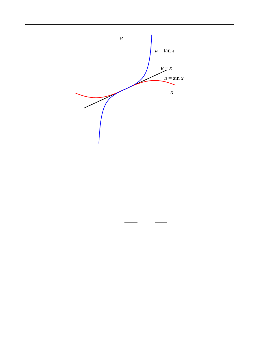
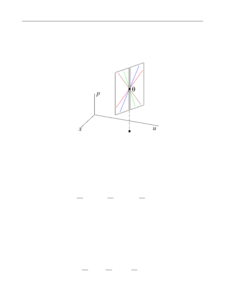
|σ| ≤ k. For example (see Fig. 1.1),
[x]
i
0
= [sin x]
i
0
for i = 0, 1, 2, but
[x]
3
0
̸= [sin x]
3
0
.
The k-jet of the function (x
− a)
m
at the point a is zero if k < m:
[(x
− a)
m
]
k
a
= [0]
k
a
.
(1.1)
The polynomial
f (a) +
∑
|σ|≤k
1
σ!
∂f
|σ|
∂x
σ
(a)(x
− a)
k
1.1. Jets
7
we shall consider as a representative of k-jet [f ]
k
a
in the given coordinates.
Let us introduce a structure of a vector space on J
k
a
M . Define a summa
of two jets and a product a jet by a real number by the following formulas:
[f ]
k
a
+ [g]
k
a
def
= [f + g]
k
a
,
λ[f ]
k
a
def
= [λf ]
k
a
.
Theorem 1.1. The k-jets
[1]
k
a
,
[x
− a]
k
a
, . . . ,
1
σ!
[(x
− a)
σ
]
k
a
(
|σ| ≤ k).
form a basis of the vector space J
k
a
M .
Proof. Due to the Taylor formula, we have:
f (x) = f (a) +
∑
|σ|≤k
1
σ!
∂f
|σ|
∂x
σ
(a)(x
− a)
k
+ o((x
− a)
k
).
and
[f ]
k
a
= f (a)[1]
k
a
+
∑
|σ|≤k
∂f
|σ|
∂x
σ
(a)
[(x
− a)
σ
]
k
a
σ!
.
Exercise 1. Prove that
dim J
k
a
M =
(
k + n
k
)
.
Definition 1.2. The union of all k-jets, i.e.,
J
1
M
def
=
∪
a
∈M
J
1
a
M
is called a space of k-jets of functions on M .
On this space we define a structure of smooth manifold with local coor-
dinates
x
1
, . . . , x
n
, u, p
σ
,
(
|σ| ≤ k)
where
x
i
([f ]
k
a
) = x
i
(a),
u([f ]
k
a
) = f (a),
p
σ
([f ]
k
a
) =
∂
|σ|
f
∂x
σ
(a)
(
|σ| ≤ k).
8
Lecture 1. Geometry of jet spaces
Figure 1.2: The map [f ]
k
Corollary 1.
dim J
k
M = n +
(
k + n
k
)
.
With functions f
∈ C
∞
(M ) we associate maps
[f ]
k
: M
→ J
k
M
where
[f ]
k
(a) = [f ]
k
a
.
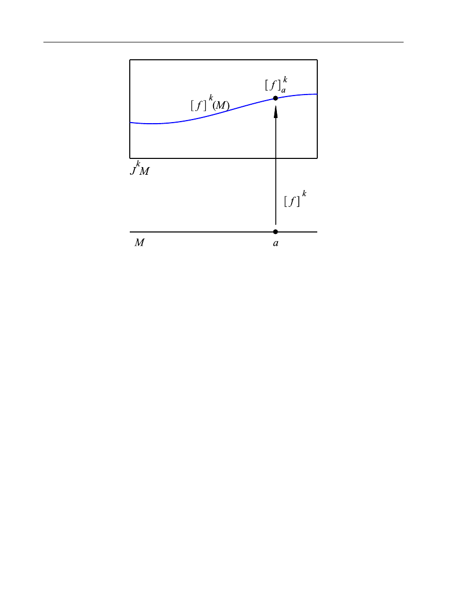
Definition 1.3. The map [f ]
k
is called the k-prolongation of the function f .
The image of M is a smooth submanifold
L
k
f
= [f ]
k
(M )
⊂ J
k
M
which we call k-graph of the function f (see Fig. 1.2).
Exercise 2. Prove that the bundles
π
k
: J
k
M
→ M,
π
k
: [f ]
k
a
7→ a
are a vector bundles.

1.2. Cartan distribution
9
1.2
Cartan distribution
Consider the following problem: describe a class of all n-dimensional submani-
folds of J
k
M that are k-graphs of functions.
Note that if L
⊂ J
k
M is a k-graph of a function, then the projection
π : L
→ M is a diffeomophism. This means that local coordinates on M can
be viewed as local coordinates on L.
On the other hand, a submanifold
L =
{u = f(x), p
σ
= g
σ
(x)
} ⊂ J
k
M,
is a k-graph of a function if and only if
g
σ
=
∂
|σ|
f
∂x
σ
,
|σ| ≤ k.
We shall describe such submanifolds in a coordinate-free form. For this
goal let’s introduce the so-called Cartan distribution.
At first,recall some facts of distributions theory.
A k-dimensional distribution P on a smooth manifold N is a «smooth»
field
P : a
∈ N 7→ P (a) ⊂ T
a
N
of k-dimensional subspaces of the tangent spaces.
There are two main ways to say that P is a smooth field, and to define a
distribution: by vector fields or by differential 1-forms.
By vector fields.
Let X
1
, . . . , X
k
be such vector fields on N that P (a) is
span by the tangent vectors X
1,a
, . . . , X
k,a
:
P (a) = Span(X
1,a
, . . . , X
k,a
).
In this case we write
P =
⟨X
1
, . . . , X
k
⟩.
We say that a vector field X belongs to P if X
a
∈ P (a) for any point
a
∈ N. Then smoothness of P means that there are local bases for P consisting
of vector fields that belong to P .
10
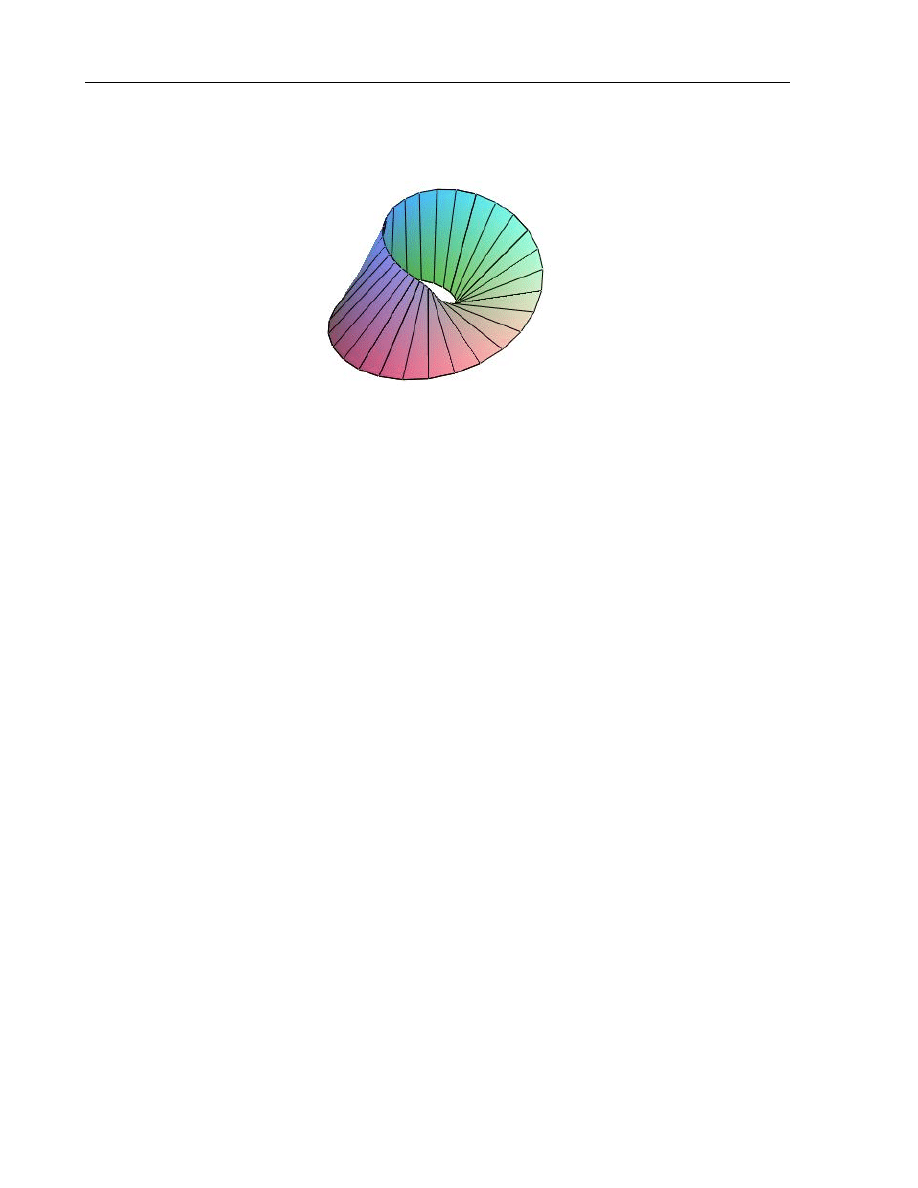
Lecture 1. Geometry of jet spaces
Figure 1.3: One-dimensional distribution on Mobius strip
We denote by D(P ) the set of all vector fields that belong to P .
By differential 1-forms. Suppose that there are n
− k differential 1-forms
ω
1
, . . . , ω
n
−k
(n = dim N ) such that a subspace P (a) is the intersection of
kernels of these forms:
P (a) =
n
−k
∩
i=1
ker ω
i,a
.
In this case we write
P =
⟨ω
1
, . . . , ω
n
−k
⟩.
The smoothness of P means that locally the distribution can be defined
by a set of differential 1-forms.
Remark 1. For general smooth manifolds distributions can be defined by vector
fields or by differential forms only locally. For example, the one-dimensional
distribution P on the Mobius strip (see Fig. 1.3) cannot be defined by a vector
field globally: each vector field which belongs to this distributions has a singular
point.

1.2. Cartan distribution
11
A submanifold L
⊂ N is said to be integral for the distribution P if
T
a
L
⊂ P (a)
for any point a
∈ L.
Return to the Cartan distribution.
Let θ
∈ J
k
M and a = π
k
(θ). Then the subspace
C
k
(θ) = Span
∪
f
∈C
∞
(M ),[f ]
k
a
=θ
T
θ
L
k
f
is called the Cartan subspace.
The distribution
C
k
: J
k
M
∋ θ 7→ C
k
(θ)
⊂ T
θ
J
k
M
is called the Cartan distribution.
By the construction, k-graphs of functions are integral manifolds of the
Cartan distribution.
Note that not any integral manifold L
⊂ J
k
M of the Cartan distribution
is a k-graph of a function. This is true if and only the projection π : L
→ M is
a diffeomophism.
Theorem 1.2. An n-dimensional smooth manifold L is a k-graph of a smooth
function on M if and only if
• L is an integral manifold of the Cartan distribution,
• the projection π : L → M is a diffeomophism.
Example 1. Consider a case when M =
R
. Then J
1
R
=
R
3
and coordinates
on J
1
R
are such functins x, u, p, that
x([f ]
1
a
) = a,
u([f ]
1
a
) = f (a),
p([f ]
1
a
) = f
′
(a).
Then the curve
L
1
f
=
{u = f(x), p = f
′
(x)
}
is a 1-graph of the function f .
12
Lecture 1. Geometry of jet spaces
Figure 1.4: Cartan subspace for n = 1
A tangent line T
θ
L
1
f
at a point θ = [f ]
1
a
is generated by the vector
∂
∂x
θ
+ f
′
(a)
∂
∂u
θ
+ f
′′
(a)
∂
∂p
θ
All possible tangent lines T
θ
L
1
f
are lines fin the plane
{du − p
θ
dx = 0
} ⊂ T
θ
(J
1
R
)
(1.2)
without the vertical line (see picture 1.4). Here a, u
θ
, p
θ
are coordinates of the
point θ. Therefore they span is plane (1.2).
So, in this case the Cartan space
C(θ) is a plane which is generated by
the vectors
∂
∂x
θ
+ p
θ
∂
∂u
θ
,
∂
∂p
θ
.
Therefore, the Cartan distribution is generated by the corresponding vec-
1.3. Contact structure on J
1
M
13
tor fields:
∂
∂x
+ p
∂
∂u
,
∂
∂p
or, equivalently, by the differential 1-form
ω
0
= du
− pdx.
This form is called Cartan form.
Figure 1.5: Cartan distribution for n = 1
1.3
Contact structure on J
1
M
Consider the case when M =
R
n
. Then J
1
R
n
=
R
2n+1
and coordinates on J
1
R
are
x
1
, . . . , u, p
1
, . . . , p
n
where
x
i
([f ]
1
a
) = a
i
,
u([f ]
1
a
) = f (a),
p
i
([f ]
1
a
) =
∂f
∂x
i
(a).
The Cartan distribution is generated by the vector fields
∂
∂x
i
+ p
i
∂
∂u
,
∂
∂p
i
(i = 1, . . . , n),

14
Lecture 1. Geometry of jet spaces
or by the differential 1-form
ω
0
= du
− p
1
dx
1
− · · · − p
n
dx
n
.
(1.3)
Recall that a contact structure on odd-dimensional smooth manifold is a
maximal non-integrable distribution of codimensional 1. This means the follow-
ing.
Let P =
⟨ω⟩ be a 2n-dimensional distribution on 2n + 1-dimensional
smooth manifold N . This distribution is called a contact structure if ω
∧(dω)
n
̸=
0.
The following theorem gives a canonical representation for contact struc-
tures.
Theorem 1.3 (G. Darboux). Let P =
⟨ω⟩ be a contact structure. There exist
local coordinates x
1
, . . . , x
n
, y
1
, . . . , y
n
, z on N such that
ω = dz
− y
1
dx
1
− · · · − y
n
dx
1
.
Since (1.3), we have
dω
0
= dq
1
∧ dp
1
+
· · · + dq
n
∧ dp
n
.
(1.4)
Therefore,
ω
0
∧ (dω
0
)
n
̸= 0
and we see that the Cartan distribution
C defines the contact structure on J
1
M .
Let θ be a point of J
1
M . A restriction of dω
0
on the Cartan space
C(θ)
defines a symplectic structure. We denote it by Ω
θ
, i.e.,
Ω
θ
= dω
0
|
C(θ)
.
1.4
Contact transformations
Definition 1.4. A diffeomophism φ : J
1
M
→ J
1
M is called contact if it
preserves the Cartan distribution.
In other words, contact diffeomorphisms are symmetries of the Cartan
distribution.

1.4. Contact transformations
15
This means that
φ
∗
(ω
0
) = λ
φ
ω
0
for a smooth function λ
φ
on J
1
M .
The following transformations are contact:
1. Translations:
(x, u, p)
7−→ (x + α, u + β, p),
where α, β are constant.
2. Scale transformations
(x, u, p)
7−→ (e
α
x, e
β
u, e
(β
−α)
p).
3. The Legendre transformation:
(x, u, p)
7−→ (p, u − xp, −x)
4. The Euler (or partial Legendre’s) transformation:
(x
1
, x
2
, u, p
1
, p
2
)
7−→ (p
1
, x
2
, u
− p
1
x
1
,
−x
1
, p
2
)
5. Shifts:
(x, u, p)
7→
(
x, u + h, p +
∂h
∂x
)
,
where h = h(x).
Important class of contact transformations can be obtained as prolonga-
tions of transformations of the space J
0
M .
Diffeomophism of the 0-jets space are called point transformations.
Let
φ : (x, u)
7→ (X(x, u), U(x, u))
be a point transformation.
Definition 1.5. The transformation
φ
(1)
: (x, u, p)
7→ (X(x, u), U(x, u), P (x, u, p))
is called the first prolongation or the prolongation of the transformation φ to
the space J
1
M if it preserves the Cartan distribution.
16
Lecture 1. Geometry of jet spaces
Exercise 3. Prove that for the first prolongation
P =
dY
dx
dX
dx
,
where
d
dx
=
∂
∂x
+ p
∂
∂u
.
1.5
Contact vector fields
Infinitesimal analogies of contact transformations are contact vector fields.
Let X be a vector field on J
1
M and let
{φ
t
} be a local translation group
of X.
Definition 1.6. The vector field X is called contact if its translation group
consists of contact transformations, i.e.
φ
∗
t
(ω
0
) = λ
t
ω
0
(1.5)
for some function λ
t
on J
1
M .
After differentiating both parts of (1.5) by t at t = 0, we get:
d
dt
t=0
φ
∗
t
(ω
0
) =
dλ
dt
t=0
ω
0
.
(1.6)
The left part of the equation is the Lie derivative L
X
(ω
0
) of the Cartan form
by the vector field X. Multiplying both parts of the last equation by the form
ω
0
we get:
L
X
(ω
0
)
∧ ω
0
= 0.
(1.7)
Find a coordinate representation of contact vector fields. For simplify our
calculations we suppose that n = 1. Let x, u, p be coordinates on J
1
M .
Let
X = a
∂
∂x
+ b
∂
∂u
+ c
∂
∂p
be a contact vector field. Here a, b, c are smooth functions on J
1
M . Using the
formula
L
X
= d
◦ ι
X
+ ι
X
◦ d,
1.6. Lie transformations
17
we get
L
X
(ω
0
) = db
− cdx − pda.
Formula (1.7) gives two differential equations on the components of X :
p
∂a
∂p
−
∂b
∂p
= 0,
∂b
∂x
− p
∂a
∂x
− c + p
(
∂b
∂u
− p
∂a
∂u
)
= 0.
Let us put
f = b
− pa.
Then
a =
−
∂f
∂p
,
b = f
− p
∂f
∂p
,
c =
∂f
∂x
+ p
∂f
∂u
and any contact vector field determines by a smooth function f and has the
following form:
X
f
=
−
∂f
∂p
∂
∂x
+
(
f
− p
∂f
∂p
)
∂
∂u
+
(
∂f
∂x
+ p
∂f
∂u
)
∂
∂p
.
Note that
ω
0
(X
f
) = f.
For arbitrary n a contact vector field has the form
X
f
=
−
n
∑
i=1
∂f
∂p
i
∂
∂x
i
+
(
f
−
n
∑
i=1
p
i
∂f
∂p
i
)
∂
∂u
+
n
∑
i=1
(
∂f
∂x
i
+ p
i
∂f
∂u
)
∂
∂p
i
for some function f .
1.6
Lie transformations
Lie transformations are generalization of contact transformations.
Definition 1.7. A diffeomophism φ : J
k
M
→ J
k
M is called a Lie transfor-
mation if it preserves the Cartan distribution
C
k
.
For k = 1 Lie transformations are contact ones.
Each Lie transformation on J
k
M can be prolonged to the space J
k+1
M .
Theorem 1.4. Any Lie transformation on J
k
M is is a (k
− 1)-th prolongation
of a contact transformation.
Lecture 2
Differential equations
2.1
Multivalued solutions
Consider a scalar k-th order differential equation on a smooth manifold M
F
(
x, v,
∂
|σ|
v
∂x
σ
)
= 0,
|σ| ≤ k.
(2.1)
This equation can be viewed as a hypersurface
E = {F (x, u, p
σ
) = 0
} ⊂ J
k
M
in the space of k-jets. This hypersurface we call an equation too.
Theorem 2.1. A function v = h(x) is a solution of equation (2.1) if and only
if its k-graph lies on the hypersurface
E.
Proof. A function v = h(x) is a solution of (2.1) if and only if
F
(
x, h(x),
∂
|σ|
h(x)
∂x
σ
)
≡ 0.
This means that L
k
h
⊂ E.
Definition 2.1. An n-dimensional integral manifold L of the Cartan distribu-
tion is called a multivalued solution of equation
E if L ⊂ E.
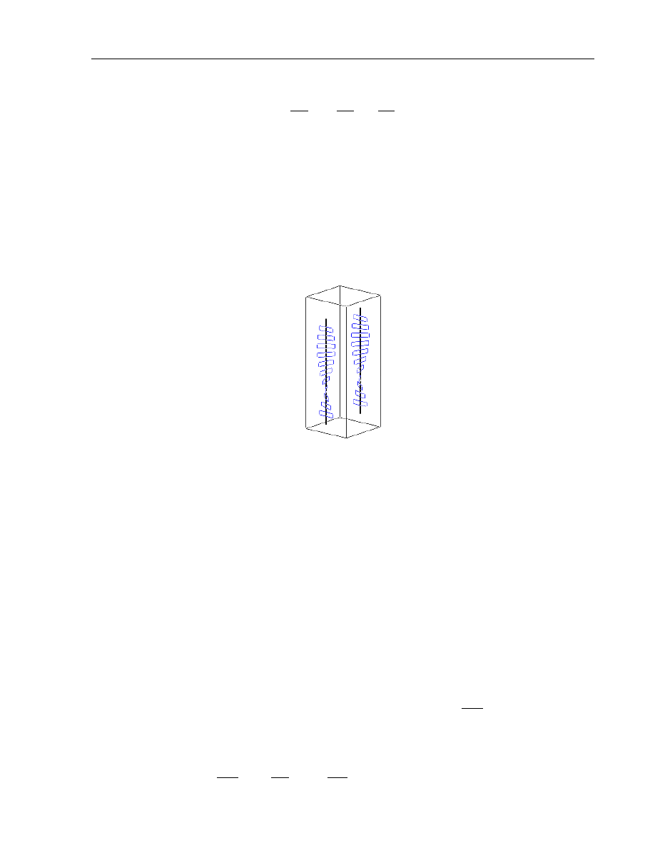
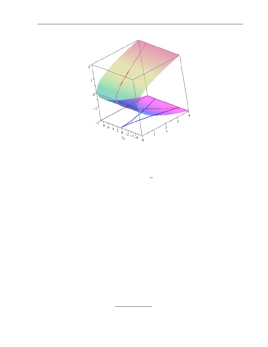
Example 2. The ordinary differential equation
(y
′
)
2
= x
(2.2)
generates the following hypersurface in J
1
R
:
E = {p
2
− x = 0}.
18
2.1. Multivalued solutions
19
Figure 2.1: Equation p
2
= x and its multivalued solution
The curve
L =
{
x = t
2
,
u =
2
3
t
3
,
p = t
}
(see Fig. 2.2) is a multivalued solution of the equation.
Exercise 4. Construct multivalued solutions of the following equation:
(y
′
)
3
− 3y
′
− y + 1 = 0.
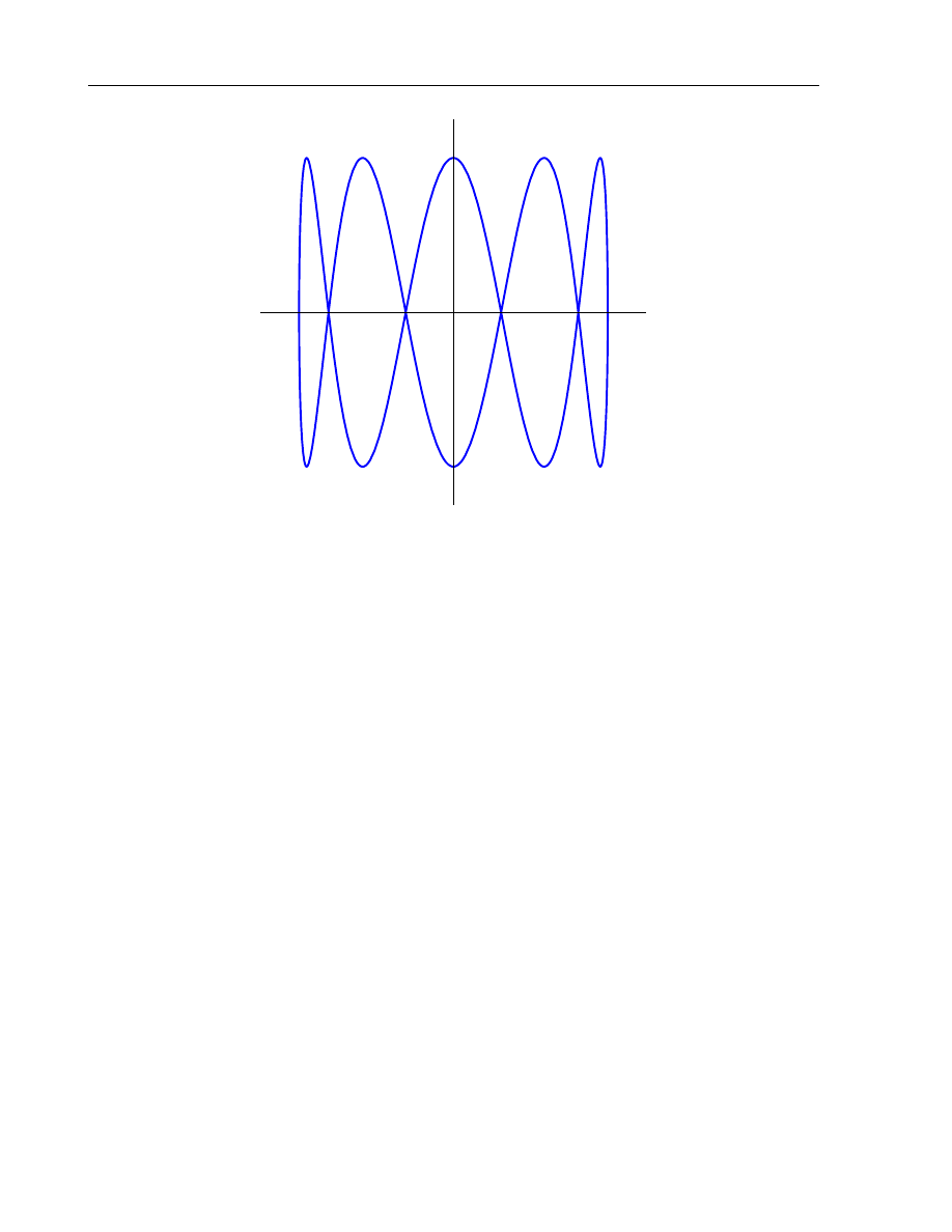
Example 3. The Lissajou figure
u = cos(at), x = sin(bt)
corresponds to a multivalued solution of the differential equation
(1
− x
2
)y
′′
+ xy
′
+ λy = 0
with λ = a
2
/b
2
.
Example 4. Spheres with radius 1 in the space
R
3
(x, y, u) are projections of
multivalued solutions of the equation
v
xx
v
yy
− v
2
xy
(1 + v
2
x
+ v
2
y
)
2
= 1.
(2.3)
into J
0
R
2
.
20
Lecture 2. Differential equations
Figure 2.2: The Lissajou figure
2.2
Lychagin’s approach to Monge-Amp`
ere equations
Let M be an n-dimensional smooth manifold and let J
1
M be the manifold of
1-jets of smooth functions on M .
The manifold J
1
M is equipped with Cartan’s distribution
C : a ∈ J
1
M
7→ C(a) ⊂ T
a
(J
1
M )
given by the differential 1-form ω
0
.
In the canonical local coordinates on J
1
M the Cartan form
ω
0
= du
− p
1
dx
1
− · · · − p
n
dx
n
.
A main idea of V. Lychagin is the following [23].
With any differential n-form ω on J
1
M we can associate a differential
operator
∆
ω
: C
∞
(M )
→ Ω
n
(M ),
which acts by the following way:
∆
ω
(v) = ω
|
L
1
v
.

2.2. Lychagin’s approach to Monge-Amp`
ere equations
21
Here L
1
v
is the 1-graph of the function v.
This construction does not cover all nonlinear second order differential
operators, but only a certain subclass of them.
Example 5. Let
ω = 3p
2
dp
− dx
(2.4)
be the differential 1-form on J
1
(
R
). The corresponding operator ∆
ω
acts as
∆
ω
(v) =
(
3(v
′
)
2
v
′′
− 1
)
dx.
(2.5)
Indeed,
∆
ω
(v) = (3p
2
dp
− dx)|
j
1
(v)(M )
= 3(v
′
)
2
d (v
′
)
− dx =
(
3(v
′
)
2
v
′′
− 1
)
dx.
Example 6. The differential 2-form
ω = dp
1
∧ dp
2
on J
1
R
2
corresponds to operator
∆
ω
(v) = d (v
x
1
)
∧ d (v
x
2
)
= (v
x
1
x
1
dx
1
+ v
x
1
x
2
dx
2
)
∧ (v
x
2
x
1
dx
1
+ v
x
2
x
2
dx
2
)
=
(
v
x
1
x
1
v
x
2
x
2
− v
2
x
1
x
2
)
dx
1
∧ dx
2
= (det Hess v) dx
1
∧ dx
2
.
where
Hess v = det
v
x
1
x
1
v
x
1
x
2
v
x
1
x
2
v
x
2
x
2
is the Hessian of the function v.
Thus,
∆
ω
(v) = (Hess v) dx
1
∧ dx
2
.
(2.6)
Example 7. The differential 3-form
ω = dx
1
∧ dp
1
∧ dp
3
(2.7)
on J
1
R
3
produces the following differential operator :
∆
ω
(v) = dx
1
∧ d (v
x
1
)
∧ d (v
x
3
) = (v
x
1
x
2
v
x
3
x
3
− v
x
1
x
3
v
x
2
x
3
) dx
1
∧ dx
2
∧ dx
3
.

22
Lecture 2. Differential equations
Example 8. The differential 2-form
ω = dp
1
∧ dx
2
− dp
2
∧ dx
1
on J
1
R
2
represents the 2-dimensional Laplace operator
∆
ω
(v) = (v
x
1
x
1
+ v
x
2
x
2
) dx
1
∧ dx
2
.
The constructed operator ∆
ω
and the equation
E
ω
=
{∆
ω
(v) = 0
} ⊂ J
2
M
are called the Monge-Amp`
ere operator and the Monge-Amp`
ere equation, re-
spectively.
The following observation justifies this definition: being written in local
canonical contact coordinates on J
1
M , the operators ∆
ω
have the same type of
nonlinearity as the Monge-Amp`
ere operators. Namely, the nonlinearity involves
the determinant of the Hesse matrix and its minors. For instance, in the case
n = 2 we get classical Monge-Amp`
ere equations
Av
xx
+ 2Bv
xy
+ Cv
yy
+ D(v
xx
v
yy
− v
2
xy
) + E = 0.
(2.8)
An advantage of this approach is the reduction of the order of the jet space:
we use the simpler space J
1
M instead of the space J
2
M where Monge-Amp`
ere
equations should be ad hoc as second-order partial differential equations [29].
The two next examples show that the constructed map «differential n-
forms»
→ «differential operators» is not a 1-to-1 map: it has a huge kernel.
Example 9. Two differential 2-forms
ω = dx
1
∧ du
and
ϖ = p
2
dx
1
∧ dx
2
on J
1
R
2
generate the same operator:
∆
ω
(v) = dx
1
∧ (v
x
1
dx
1
+ v
x
2
dx
2
) = v
x
2
dx
1
∧ dx
2
,
∆
ϖ
(v) = v
x
2
dx
1
∧ dx
2
.
Example 10. Any differential n-form
ω = ω
0
∧ α + dω
0
∧ β
(2.9)
on J
1
M , where α
∈ Ω
n
−1
(
J
1
M
)
, β
∈ Ω
n
−2
(
J
1
M
)
and ω
0
is the Cartan form,
gives the zero operator.

2.3. Contact transformations of Monge-Amp`
ere equations
23
This kernel consists of differential forms that vanish on any integral man-
ifold of the Cartan distribution. Due to Lepage’s theorem [24], all such forms
have form (2.9). They generate a graded ideal
I
∗
=
⊕
s
≥0
I
s
,
I
s
⊂ Ω
s
(J
1
M ) of the exterior algebra Ω
∗
(J
1
M ).
Definition 2.2. Elements of the quotient module Ω
s
ε
(J
1
M ) = Ω
s
(J
1
M )/I
s
are
called effective s-forms.
By ω
ε
denote the corresponding to ω class in Ω
s
ε
(J
1
M ): ω
ε
= ω + I
s
.
Suppose that n = 2 and find a coordinate representation of effective 2-
forms.
For any element of the factor module Ω
2
ε
, one can choose a unique rep-
resentative ω
∈ Ω
2
(J
1
M ) such that X
1
⌋ω = 0 and ω ∧ dω
0
= 0. Here X
1
is a contact vector fields with generating function 1. In the local Darboux
coordinates such representatives have the form
ω =Edq
1
∧ dq
2
+ B (dq
1
∧ dp
1
− dq
2
∧ dp
2
) +
(2.10)
Cdq
1
∧ dp
2
− Adq
2
∧ dp
1
+ Ddp
1
∧ dp
2
,
where A, B, C, D and E are smooth functions on J
1
M .
We identify effective forms as elements of the factor module Ω
2
ε
(J
1
M ) with
differential forms of type (2.10) and also call such differential forms effective.
Form (2.10) corresponds to equation (2.8).
2.3
Contact transformations of Monge-Amp`
ere equations
Let φ : J
1
M
→ J
1
M be a contact transformation. This transformation pre-
serves the ideal I
∗
: φ
∗
(I
s
) = I
s
, and therefore determines a map of effective
forms:
φ
∗
: ω + I
s
7→ φ
∗
(ω) + I
∗
.
But φ, in general, does not preserves the Cartan form ω
0
, and therefore,
does not acts directly on representatives of the effective forms. Thus we shall
define the action φ on ω by taking the effective part φ
∗
(ω)
ε
.

24
Lecture 2. Differential equations
Note that, for any contact transformation and any integral manifold of
the Cartan distribution L
⊂ J
1
M we have:
φ
∗
(ω)
ε
|
L
= ω
|
φ(L)
,
Hence, if L is a multivalued solution of the equation
E
φ
∗
(ω)
ε
, then φ(L) is a
multivalued solution of the equation
E
ω
.
Definition 2.3. Two Monge-Amp`
ere equations
E
ω
and
E
ϖ
are contact equiva-
lent if and only if there exists a contact transformation φ and a nonvanishing
function λ
φ
∈ C
∞
(J
1
M ) such that
ω = λ
φ
φ
∗
(ϖ)
ε
.
As a corollary of our interpretation of Monge-Amp`
ere equations we get
the following theorem.
Theorem 2.2 (Sophus Lie). The class of Monge-Amp`
ere equations is closed
with respect to contact transformations.
Example 11. The Legendre transformation
φ : (x, u, p)
7→ (p, u − px, −x)
transforms the form (2.4) to the form
φ
∗
(ω) = 3x
2
dx
− dp.
Then the non-linear equation
3(v
′
)
2
v
′′
− 1 = 0
turns to the following linear equation:
v
′′
= 3x
2
.
Example 12. The Von Karman equation
v
x
1
v
x
1
x
1
− v
x
2
x
2
= 0
(2.11)
becomes linear equation
x
1
v
x
2
x
2
+ v
x
1
x
1
= 0
(2.12)
after Legendre transformation (2.14). The last equation is known as the Tric-
comi equation.

2.3. Contact transformations of Monge-Amp`
ere equations
25
Example 13 (The Monge-Ampere Equation). This equation has the form
Hess v = 1
and generated by the effective differential 2-form
ω = dp
1
∧ dp
2
− dx
1
∧ dx
2
.
After the Euler transformation
φ : (x
1
, x
2
, u, p
1
, p
2
)
7→ (p
1
, x
2
, u
− p
1
x
1
,
−x
1
, p
2
, ).
it becomes
ω = dx
2
∧ dp
1
− dx
1
∧ dp
2
,
and corresponds to the Laplace equation
v
x
1
x
1
+ v
x
2
x
2
= 0.
(2.13)
Example 14 (Quasilinear equations). Let’s consider a quasi-linear equation of
the form:
A (v
x
, v
y
) v
xx
+ 2B (v
x
, v
y
) v
xy
+ C (v
x
, v
y
) v
yy
= 0.
This equation is represented by the following effective form
ω = B (p
1
, p
2
) (dx
1
∧ dp
1
− dx
2
∧ dp
2
)+ C (p
1
, p
2
) dx
1
∧dp
2
−A (p
1
, p
2
) dx
2
∧dp
1
.
After the Legendre transformation
φ : (x
1
, x
2
, u, p
1
, p
2
)
7→ (p
1
, p
2
, u
− p
1
x
1
− p
2
x
2
,
−x
1
,
−x
2
, )
(2.14)
we get the following effective form
φ
∗
(ω) = B (
−x
1
,
−x
2
) (dx
1
∧ dp
1
− dx
2
∧ dp
2
) +
− A (−x
1
,
−x
2
) dx
1
∧ dp
2
+ C (
−x
1
,
−x
2
) dx
2
∧ dp
1
,
which corresponds to linear equation:
−A (−x
1
,
−x
2
) v
x
2
x
2
+ 2B (
−x
1
,
−x
2
) v
x
1
x
2
− C (−x
1
,
−x
2
) v
x
1
x
1
= 0.

Lecture 3
Classification of Monge-Amp`
ere
equations
3.1
The Sophus Lie problem
The problem of equivalence and classification of the Monge-Amp`
ere equations
with two independent variables x and y goes back to Sophus Lie’s papers from
the 1870s and 1880s [20, 21, 22].
Lie have raised the following problem.
Find equivalence classes of nonlinear second-order differential equations
with respect to the group of contact transformations.
The important steps in a solution of this problem were made by Darboux
[2, 3, 4] and Goursat [?, ?, ?], who had basically treated the hyperbolic Monge-
Amp`
ere equations.
Lie himself had found conditions to transform a Monge-Amp`
ere equation
to a quasilinear one and to some linear equation with constant coefficients. But
a complete proof of Lie’s theorems had never been published. A problem of
reducibility of hyperbolic and elliptic Monge-Amp`
ere equations, whose coeffi-
cients do not depend on the variable v (they call such equations symplectic), to
the equations with constant coefficients was solved by Lychagin and Rubtsov in
1983 [26].
26

3.2. Geometry of Monge-Amp`
ere equations on two-dimensional manifolds
27
3.2
Geometry of Monge-Amp`
ere equations on two-dimensional
manifolds
The Monge-Amp`
ere equations on two-dimensional manifolds possess remark-
able geometric structures. We consider them for the general and symplectic
equations separately.
In what follows, we suppose that n = 2 and consider classical Monge-
Amp`
ere equations (2.8) only.
With any effective differential 2-form ω one can associate a smooth func-
tion Pf(ω) on J
1
M as follows [26]:
Pf(ω)Ω
∧ Ω = ω ∧ ω.
(3.1)
This function is called Pfaffian of ω.
If ω has the form (2.10) then
Pf(ω) = DE
− AC + B
2
.
We say that the Monge-Amp`
ere equation E
ω
is hyperbolic, elliptic or
parabolic at a domain
D ⊂ J
1
M if the function Pf(ω) is negative, positive or
zero at each point of
D, respectively.
If the Pfaffian changes a sign in some points of
D, then the equation E
ω
is called a mixed type equation.
The hyperbolic and elliptic equations are called nondegenerate.
Define a non-holonomic field endomorphisms A
ω
which is associated with
effective form ω.
Since the 2-form Ω
a
is non-degenerated on the Cartan distribution
C(a),
the operator A
ω
a
is uniquely defined by the following formula [26]:
A
ω
a
X
a
⌋ Ω
a
= X
a
⌋ ω
a
.
(3.2)
Here X
a
∈ C(a).
To find a coordinate representation of the operator A
ω
consider the fol-
lowing basis of the module D(
C):
d
dq
1
def
=
∂
∂q
1
+ p
1
∂
∂u
,
d
dq
2
def
=
∂
∂q
2
+ p
2
∂
∂u
,
∂
∂p
1
,
∂
∂p
2
(3.3)

28
Lecture 3. Classification of Monge-Amp`
ere equations
Then, in this basis, one has the form
A
ω
=
B
−A
0
−D
C
−B
D
0
0
E
B
C
−E
0
−A −B
(3.4)
in basis (3.3).
The square of operator A
ω
is scalar and
A
2
ω
+ Pf(ω) = 0.
(3.5)
Remark that the operator A
ω
is symmetric with respect to Ω, i.e.,
Ω(A
ω
X, Y ) = Ω(X, A
ω
Y )
(3.6)
for any X, Y
∈ D(C) [26].
It is clear that effective forms ω and hω, where h is any nonvanishing
function, define the same equation.
Therefore, for a non-degenerate equation E
ω
the form ω can be normed
in such a way that
| Pf(ω)| = 1.
Then, due to (3.5), the hyperbolic and elliptic equations generate a prod-
uct structure
A
ω,a
= 1
and a complex structure
A
ω,a
=
−1
on
C(a) respectively on the Cartan space C(a) [25].
Thus, a non-degenerate Monge-Amp`
ere equation generates two 2-
dimensional distributions on J
1
M , which are formed by eigenspaces of the
operator A
ω
a
.
These eigenspaces
C
+
(a) and
C
−
(a) correspond to the eigenvalues 1 and
−1 or ι and −ι in hyperbolic or elliptic cases respectively. Here ι =
√
−1.
The distributions
C
+
and
C
−
are called characteristic.
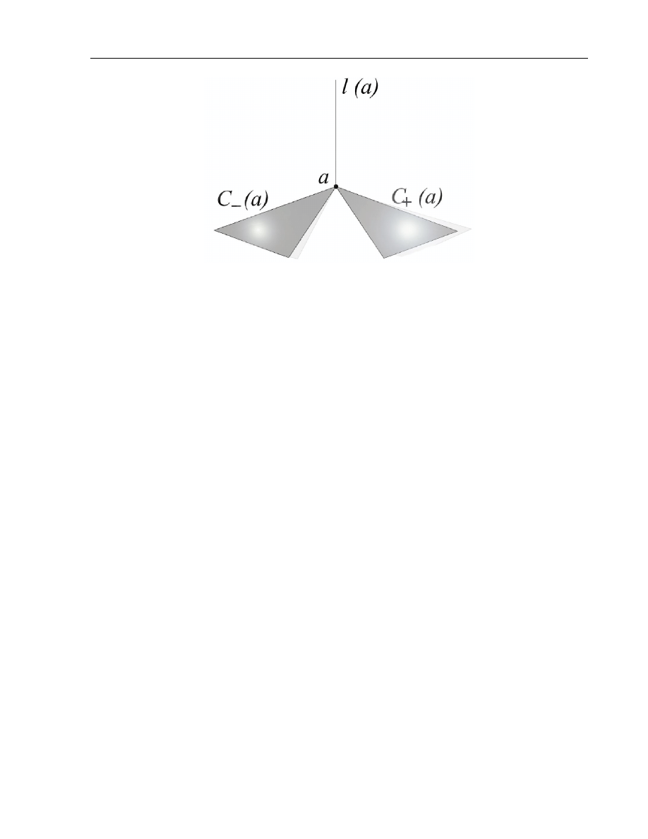
3.2. Geometry of Monge-Amp`
ere equations on two-dimensional manifolds
29
Figure 3.1: 3-tuple almost product structure for hyperbolic equations
The characteristic distributions are real for the hyperbolic equations and
complex for the elliptic ones. For the elliptic equations they are also complex
conjugate.
Moreover, planes
C
+
(a) and
C
−
(a) are skew-orthogonal with respect to
the symplectic structure Ω
a
.
On each of them the 2-form Ω
a
is nondegenerate. It is easy to see that the
first derivatives of the characteristic distributions
C
(1)
±
=
C
±
+ [
C
±
,
C
±
] are three-
dimensional. Therefore their intersection l =
C
(1)
+
∩ C
(1)
−
is a one-dimensional
distribution, which is transversal to
C [25].
Hence, for the hyperbolic equations the tangent space T
a
(J
1
M ) splits into
the direct sum
T
a
J
1
M =
C
+
(a)
⊕ l(a) ⊕ C
−
(a).
(3.7)
at each point a
∈ J
1
M (see Fig. 3.1) [25].
For elliptic equations we have the similar decomposition of the complexi-
fication of T
a
J
1
M . But the distributions l is real also in this case.
We say that a non-degenerate equation is called regular if the derivatives
C
(k)
±
(k = 1, 2, 3) of the characteristic distributions are distributions too.
The above decomposition of the tangent bundle allows us to construct
a decomposition of the de Rham complex, which is generated by an equation
[10, 25].
Denote the distributions
C
+
, l, and
C
−
by P
1
, P
2
, and P
3
, respectively.

30
Lecture 3. Classification of Monge-Amp`
ere equations
Let D(J
1
M ) be the module of vector fields on J
1
M , and let D
j
be the
module of vector fields from the distribution P
j
. Define the following submod-
ules of Ω
s
(J
1
M ):
Ω
s
i
=
{α ∈ Ω
s
(J
1
M )
| X⌋α = 0 ∀ X ∈ D
j
, j
̸= i} (i = 1, 2, 3).
We get the following decomposition of the module of differential s-forms on
J
1
M :
Ω
s
(J
1
M ) =
⊕
|k|=s
Ω
k
,
(3.8)
where k =(k
1
, k
2
, k
3
) is a multi-index, k
i
∈ {0, 1, . . . , dim P
i
}, |k| = k
1
+k
2
+k
3
,
Ω
k
=
∑
j
1
+j
2
+j
3
=
|k|
α
j
1
∧ α
j
2
∧ α
j
3
, where α
j
i
∈ Ω
k
i
i
⊂
3
⊗
i=1
Ω
k
i
i
.
Three first terms of this decomposition are shown on the diagram (see
Fig. 3.2).
The exterior differential also splits into the direct sum of operators
d =
⊕
|t|=1
d
t
,
where
d
t
: Ω
k
→ Ω
k+t
.
Theorem 3.1. 1. The operators d
t
are differentiations, i.e. the Leibnitz rule
holds:
d
t
(α
∧ β) = d
t
α
∧ β + (−1)
deg α
α
∧ d
t
β,
(3.9)
where α
∈ Ω
k
and β
∈ Ω
i
.
2. If the sum of negative components of the multi-index t less than
−1
then d
t
= 0.
3. If the multi-index t contains one negative component and this compo-
nent is
−1 then operator d
t
is a C
∞
(N )-homomorphism, i.e.,
d
t
(f α) = f d
t
α
(3.10)
for any dunction f and any differential form α
∈ Ω
k
.
3.2. Geometry of Monge-Amp`
ere equations on two-dimensional manifolds
31
Figure 3.2: Decomposition of the de Rham complex on J
1
M
Due to this theorem, we have the following eight homomorphisms:
d
−1,1,1
,
d
1,
−1,1
,
d
1,1,
−1
,
d
0,
−1,2
,
d
2,
−1,0
,
d
−1,0,2
,
d
2,0,
−1
d
2,0,
−1
.
and four of them are zero. The nontrivial homomorphisms are the following:
d
−1,1,1
, d
1,1,
−1
, d
2,0
−1
, and d
−1,0,2
.
Consider a case
t = 1
j
+ 1
k
− 1
s
.
Then the differential d
t
is a C
∞
(N )-homomorphisn. Due to Leibnitz’s
rule, this differential is completely defined by its values on Ω
1
(N ).

32
Lecture 3. Classification of Monge-Amp`
ere equations
Note that
d
1
j
+1
k
−1
s
: Ω
1
q
→ 0,
if q
̸= s. Therefore a non-trivial d
1
j
+1
k
−1
s
is a restriction to the module Ω
1
s
:
d
1
j
+1
k
−1
s
: Ω
1
s
→ Ω
1
j
∧ Ω
1
k
.
In other words, these homomorphisms define tensor fields of a type (2,1)
on N . We denote them by τ
1
j
+1
k
−1
s
:
τ
1
j
+1
k
−1
s
∈ Ω
1
j
∧ Ω
1
k
⊗ D
s
.
Note that
τ
1
j
+1
k
−1
s
: Ω
1
s
→ Ω
1
j
∧ Ω
1
k
coinsides with operator d
1
j
+1
k
−1
s
.
Tensor fields τ
1
j
+1
k
−1
s
are differential invariants of Monge-Amp`
ere equa-
tions.
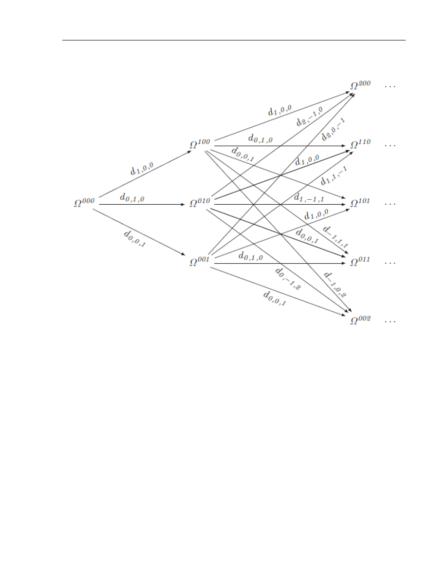
So, we have four tensors of (2,1)–type:
τ
2,
−1,0
,
τ
0,
−1,2
,
τ
−1,1,1
and
τ
1,1,
−1
.
(3.11)
Example 15. Coordinate representation of the tensor invariants for the hyper-
bolic Monge-Amp`
ere equations
v
xy
= f (x, y, v, v
x
, v
y
) ,
(3.12)
3.3. The Laplace forms
33
has the following form:
τ
−1,1,1
= (f f
p
2
p
2
dq
1
∧ du − f
p
2
p
2
dp
2
∧ du − p
1
f
p
2
p
2
dq
1
∧ dp
2
− p
2
f
p
2
p
2
dq
2
∧ dp
2
+
(f
u
− p
2
f
p
2
u
+ f
p
1
f
p
2
− ff
p
1
p
2
− f
q
2
p
2
) dq
2
∧ du+
(p
1
f
u
− p
1
p
2
f
p
2
u
− p
2
f f
p
2
p
2
+ p
1
f
p
1
f
p
2
− p
1
f f
p
1
p
2
− p
1
f
q
2
p
2
) dq
1
∧ dq
2
)
⊗
∂
∂p
1
,
τ
1,1,
−1
= (f f
p
1
p
1
dq
2
∧ du − f
p
1
p
1
dp
1
∧ du − p
1
f
p
1
p
1
dq
1
∧ dp
1
− p
2
f
p
1
p
1
dq
2
∧ dp
1
+
(f
u
+ f
p
1
f
p
2
− p
1
f
p
1
u
− ff
p
1
p
2
− f
q
1
p
1
) dq
1
∧ du+
(
−p
2
f
u
− p
2
f
p
1
f
p
2
+ p
1
p
2
f
p
1
u
+ p
2
f f
p
1
p
2
+ p
1
f f
p
1
p
1
+ p
2
f
q
1
p
1
) dq
1
∧ dq
2
)
⊗
∂
∂p
2
,
τ
2,
−1,0
= (dq
1
∧ dp
1
− f
p
2
dq
1
∧ du + (p
2
f
p
2
− f) dq
1
∧ dq
2
)
⊗
(
∂
∂u
+ f
p
2
∂
∂p
1
+ f
p
1
∂
∂p
2
)
,
τ
0,
−1,2
= (dq
2
∧ dp
2
− f
p
1
dq
2
∧ du − (p
1
f
p
1
− f) dq
1
∧ dq
2
)
⊗
(
∂
∂u
+ f
p
2
∂
∂p
1
+ f
p
1
∂
∂p
2
)
.
3.3
The Laplace forms
Let’s define a bracket
⟨·, ·⟩ by the formula
⟨α ⊗ X, β ⊗ Y ⟩ = (Y ⌋α) ∧ (X⌋β)
for tensors α
⊗ X and β ⊗ Y .
Then differential 2-forms
λ
+
=
⟨τ
0,
−1,2
, τ
1,1,
−1
⟩ ,
λ
−
=
⟨τ
2,
−1,0
, τ
−1,1,1
⟩ .
(3.13)
we call Laplace forms or Laplace invariants of the Monge-Amp`
ere equations
E
ω
.
Remark 2. For the elliptic equations the Laplace forms are complex conjugate.

34
Lecture 3. Classification of Monge-Amp`
ere equations
Example 16. For equation (3.12), the Laplace forms have the following coor-
dinate representation:
λ
−
=f
p
2
p
2
(f
p
1
dq
1
∧ du − dq
1
∧ dp
2
) +
(f
u
− p
2
f
p
2
u
+ f
p
1
f
p
2
− p
2
f
p
1
f
p
2
p
2
− ff
p
1
p
2
− f
q
2
p
2
) dq
1
∧ dq
2
,
(3.14)
λ
+
=f
p
1
p
1
(f
p
2
dq
2
∧ du − dq
2
∧ dp
1
) +
(
−f
u
+ p
1
f
p
1
u
− f
p
1
f
p
2
+ p
1
f
p
2
f
p
1
p
1
+ f f
p
1
p
2
+ f
q
1
p
1
) dq
1
∧ dq
2
.
(3.15)
In particular, for linear equation
v
xy
= a(x, y)v
x
+ b(x, y)v
y
+ c(x, y)v + g(x, y),
(3.16)
the Laplace forms are
λ
−
= kdx
∧ dy and
λ
+
=
−hdx ∧ dy,
(3.17)
where
k = ab + c
− b
y
h = ab + c
− a
x
(3.18)
are the classical Laplace invariants. This observation justifies our definition.
Remark that the classical Laplace invariants (3.18) of equation (3.16) are
not absolute invariants in contrast to the forms λ
±
.
Example 17. For the linear elliptic equation
v
xx
+ v
yy
= a(x, y)v
x
+ b(x, y)v
y
+ c(x, y)v + g(x, y)
(3.19)
the Laplace forms are
λ
±
=
1
4
(
b
x
− a
y
±
(
1
2
(a
2
+ b
2
) + 2c
− a
x
− b
y
)
ι
)
dx
∧ dy.
(3.20)
The coefficients
K = b
x
− a
y
,
and
H =
1
2
(a
2
+ b
2
) + 2c
− a
x
− b
y
(3.21)
of these forms are the Cotton invariants [1].

3.4. Contact linearization of the Monge-Ampere equations
35
3.4
Contact linearization of the Monge-Ampere equations
Consider the following problem:
Find a class of the Monge-Amp`
ere equations that are locally contact equiv-
alent to the linear equations
v
xx
± v
yy
= a(x, y)v
x
+ b(x, y)v
y
+ c(x, y)v + g(x, y).
(3.22)
A solution of the problem can be conveniently formulated in terms of the
Laplace forms.
We consider three possible cases.
3.4.1
λ
+
= λ
−
= 0
It is well known that if the classical Lagrange invariants h and k of a linear
hyperbolic equation are zero, then the equation can be reduced to the wave
equation (see [?], for example).
Similar statement is true for the Monge-Amp`
ere equations.
Theorem 3.2 ([13]). A hyperbolic Monge-Amp`
ere equation is locally contact
equivalent to the wave equation v
xy
= 0 if and only if its Laplace invariants are
zero: λ
+
= λ
−
= 0.
Corollary 2. The equation
v
xy
= f (x, y, v, v
x
, v
y
)
is locally contact equivalent to the wave equation v
xy
= 0 if and only if the
function f has the following form:
f = φ
y
v
x
+ φ
x
v
y
+ (φ
v
+ Φ
v
)v
x
v
y
+ R,
where the function R = R(x, y, v) satisfies to the following ordinary linear
differential equation:
R
v
= (φ
v
+ Φ
v
)R + φ
xy
− φ
x
φ
y
.
This equation can be solved:
R = e
φ+Φ
(∫
(φ
xy
− φ
x
φ
y
)e
−φ−Φ
dv + g
)
.
Here φ = φ(x, y, v), Φ = Φ(v), and g = g(x, y) are arbitrary functions.

36
Lecture 3. Classification of Monge-Amp`
ere equations
Theorem 3.3 ([13]). An elliptic Monge-Amp`
ere equation is locally contact
equivalent to the Poisson equation v
xx
+ v
yy
= f (x, y) if and only if its Laplace
invariants are zero: λ
+
= λ
−
= 0.
If, in addition, coefficients of the Monge-Amp`
ere equation are analytic
functions, then the equation is locally contact equivalent to the Laplace equation
v
xx
+ v
yy
= 0.
3.4.2
λ
+
̸= 0 and λ
−
̸= 0
Note that for the Laplace invariants of the linear equations (see (3.17) and
(3.20)) the following conditions:
λ
+
∧ λ
+
= 0,
λ
−
∧ λ
−
= 0,
λ
+
∧ λ
−
= 0,
and
dλ
+
= dλ
−
= 0 (3.23)
hold.
Hence, for the Monge-Amp`
ere equations that are locally contact equiva-
lent to equation (3.22) this is also true.
It follows from the following Theorem that conditions (3.23) are sufficient.
Theorem 3.4 ([10, 13]). Suppose λ
+
̸= 0 and λ
−
̸= 0. A nondegenerate
Monge-Amp`
ere equation is locally contact equivalent to equation (3.22) if and
only if conditions (3.23) hold.
3.4.3
One of the Laplace forms is zero and the another one is not
Due to Remark 2, this case realizes only for the hyperbolic equations.
For definiteness, suppose that λ
−
= 0 and λ
+
̸= 0. We shall suppose
λ
+
∧ λ
+
= 0 because this condition holds for the linear equations. This means
that λ
+
= η
−
∧ ϑ
+
, where η
−
∈ Ω
001
and ϑ
+
∈ Ω
100
are differential 1-forms.
Theorem 3.5 (see [13]). Suppose that one of the Laplace forms is zero and the
another one, say λ
+
, is not. A hyperbolic Monge-Amp`
ere equation is locally
contact equivalent to a linear equation if and only if dλ
+
= 0, λ
+
= η
−
∧ ϑ
+
,
and the distribution
F⟨ϑ
+
⟩ is completely integrable.
3.5. The Hunter-Saxton equation
37
3.5
The Hunter-Saxton equation
Consider the Hunter-Saxton equation
v
tx
= vv
xx
+ κv
2
x
,
(3.24)
where κ is a constant. This equation is hyperbolic, and it has applications in
the theory of a director field of a liquid crystal [5].
The corresponding effective differential 2-form and the operator A
ω
are
the following:
ω = 2udq
2
∧ dp
1
+ dq
1
∧ dp
1
− dq
2
∧ dp
2
− 2κp
2
1
dq
1
∧ dq
2
and
A
ω
=
1
2u
0
0
0
−1
0
0
0
−2κp
2
1
1
0
2κp
2
1
0
2u
−1
.
Let us choice the following bases in the module of vector fields on J
1
M :
X
1
=
∂
∂q
1
+ p
1
∂
∂u
+ κp
2
1
∂
∂p
2
,
X
2
=
∂
∂p
1
+ u
∂
∂p
2
,
Z =
∂
∂u
+ (2 κ
− 1) p
1
∂
∂p
2
,
Y
1
=
∂
∂q
2
+ κp
2
1
∂
∂p
1
− u
∂
∂q
1
+ (p
2
− up
1
)
∂
∂u
,
Y
2
=
∂
∂p
2
.
The dual basis of the module of differential 1-forms is
α
1
= dq
1
+ udq
2
,
α
2
= dp
1
− κp
2
1
dq
2
,
θ = du
− p
1
dq
1
− p
2
dq
2
,
β
1
= dq
2
,
β
2
= dp
2
+ (1
− 2κ) p
1
du+ (κ
−1) p
2
1
dq
1
+ (2κ
− 1) p
1
p
2
dq
2
− udp
1
.

38
Lecture 3. Classification of Monge-Amp`
ere equations
The vector fields X
1
, X
2
and Y
1
, Y
2
form bases of the modles D(
C
+
) and
D(
C
−
) respectively.
Tensor invariants of equation (3.24) have the form:
τ
−1,1,1
=
− (p
1
dq
1
∧ dq
2
+ dq
2
∧ du) ⊗
(
∂
∂q
1
+ p
1
∂
∂u
+ κp
2
1
∂
∂p
2
)
,
τ
1,1,
−1
= 2( κ
− 1)
(
κp
3
1
dq
1
∧ dq
2
+ κp
2
1
dq
2
∧ du −
dp
1
∧ du − p
1
dq
1
∧ dp
1
− p
2
dq
2
∧ dp
1
)
⊗
∂
∂p
2
,
τ
2,
−1,0
=
(
dq
1
∧ dp
1
− κp
2
1
dq
1
∧ dq
2
+ udq
2
∧ dp
1
)
⊗
(
∂
∂u
+ (2 κ
− 1) p
1
∂
∂p
2
)
,
τ
0,
−1,2
=
(
dq
2
∧ dp
2
+ (1
− 2κ) p
1
dq
2
∧ du + (1 − κ) p
2
1
dq
1
∧ dq
2
− udq
2
∧ dp
1
)
⊗
(
∂
∂u
+ (2 κ
− 1) p
1
∂
∂p
2
)
.
Then the Laplace forms for the Hunter-Saxton equation are
λ
−
=
−dq
2
∧ dp
1
,
λ
+
= 2 (1
− κ) dq
2
∧ dp
1
.
Due to Theorem 3.4, the equation is linearized. The required transformation
has the form
Q
1
= κq
2
+
1
p
1
,
Q
2
= q
2
,
U = u
− p
1
q
1
,
P
1
= q
1
p
2
1
,
P
2
= p
2
− κq
1
p
2
1
.
This transformation takes the effective form ω to the form
Ω = dQ
1
∧ dP
1
− dQ
2
∧ dP
2
+
(
2(2κ
− 1)P
1
κQ
2
− Q
1
+
2U
(κQ
2
− Q
1
)
2
)
dQ
1
∧ dQ
2
.
The corresponding linear equation is the Euler-Poisson equation
U
Q
1
Q
2
=
2κ
− 1
Q
1
− κQ
2
U
Q
1
−
1
(Q
1
− κQ
2
)
2
U.

Bibliography
[1] Cotton, E.: Sur les invariants diff´
erentiels de quelques ´
equations linearies aux
d´
eriv´
ees partielles du second ordre. Ann. Sci. Ecole Norm. Sup. 17, 211—244
(1900)
[2] Darboux, G.: Le¸cons sur la th´
eorie g´
en´
erale des surfaces. Vol. I. Paris,
Gauthier-Villars, Imprimeur–Libraire, 1887, vi+514 pp.
[3] Darboux, G.: Le¸cons sur la th´
eorie g´
en´
erale des surfaces. Vol. II. Paris,
Gauthier-Villars, 1915, 579 pp.
[4] Darboux, G.: Le¸cons sur la th´
eorie g´
en´
erale des surfaces. Vol. III. Paris,
Gauthier-Villars at fils, Imprimeur– Libraire, 1894, viii+512 pp.
[5] Hunter J.K., Saxton R.: Dynamics of director fields. SIAM J. Appl. Math.
51(6), 1498–1521 (1991)
[6] Kushner, A.G.: Chaplygin and Keldysh normal forms of Monge-Amp`
ere
equations of variable type. Mathem. Zametki 52(5) 63–67, (1992)(Russian).
English translation in Mathematical Notes 52(5), 1121–1124 (1992)
[7] Kushner, A.G.: Classification of mixed type Monge-Amp`
ere equations. In:
Pr`
astaro, A., Rassias, Th.M. (ed) Geometry in Partial Differential Equa-
tions. Singapore New-Jersey London Hong-Kong, World Scientific, 173–188
(1993)
[8] Kushner, A.G.: Symplectic geometry of mixed type equations. In: Lychagin,
V.V. (ed) The Interplay beetween Differential Geometry and Differential
Equations. Amer. Math. Soc. Transl. Ser. 2, 167, 131–142 (1995)
39

40
Bibliography
[9] Kushner, A.G.: Monge–Amp`
ere equations and e-structures. Dokl. Akad.
Nauk 361(5), 595–596 (1998) (Russian). English translation in Doklady
Mathematics, 58(1), 103–104 (1998)
[10] Kushner, A.G.: Almost product structures and Monge-Amp`
ere equations.
Lobachevskii Journal of Mathematics, http://ljm.ksu.ru 23, 151–181
(2006)
[11] Kushner, A.G.: Symplectic classification of elliptic Monge-Amp`
ere oper-
ators. Proceedings of The 4-th International Colloquium "Mathematics in
Engineering and Numerical Physics" October 6–8, 2006, Bucharest, Roma-
nia, pp. 87–94. Balkan Society of Geometers, Geometry Balkan Press (2007)
[12] Kushner, A.G.: Symplectic classification of hyperbolic Monge-Amp`
ere op-
erators. Proceedings of Astrakhan State Technical University, 1(36), 15–18
(2007)
[13] Kushner, A.G.: A contact linearization problem for Monge-Amp`
ere equa-
tions and Laplace invariants. Acta Appl. Math. 101(1–3), 177–189 (2008)
[14] Kushner, A.G.: Contact linearization of nondegenerate Monge-Amp`
ere
equations. Izv. Vyssh. Uchebn. Zaved. Mat., no 4, 43–58 (2008) English
translation in Russian Math. (Iz. VUZ) 52(4), 38–52 (2008)
[15] Kushner, A.G.: Contact linearization of Monge-Amp`
ere equations and
Laplace’s Invariants. Dokl. Akad. Nauk, 422(5), 597–600 (2008) (Russian).
English translation in Doklady Mathematics, 78(2), 751—754 (2008)
[16] Kushner, A.G.: Transformation of hyperbolic Monge–Amp`
ere equations
into linear equations with constant coefficients. Dokl. Akad. Nauk 423(5),
609–611 (2008) (Russian). English translation in Doklady Mathematics, 78
3, 907—909 (2008)
[17] Kushner, A.G.: Contact equivalence of Monge-Amp`
ere equations to linear
equations with constant coefficients. Acta Appl. Math. (to be published)

Bibliography
41
[18] Kushner, A.G., Lychagin, V.V., Rubtsov, V.N.: Contact geometry and
nonlinear differential equations. Encyclopedia of Mathematics and Its Ap-
plications 101, Cambridge University Press, Cambridge, 2007, xxii+496 pp.
[19] Laplace, P.S.: Recherches sur le calcul int´
egrals aux diff´
erences partielles.
M´
emoires de l’Acad´
emie royale des Sciences de Paris 23 24 (1773). Reprinted
in: Laplace, P.S.: Oevre compl`
etes, t. IX, Gauthier-Villars, Paris, 1893;
English Translation, New York, 1966.
[20] Lie, S.: Ueber einige partielle Differential-Gleichungen zweiter Orduung,
Math. Ann. 5, 209–256 (1872)
[21] Lie,
S.:
Begrundung
einer
Invarianten-Theorie
der
Beruhrungs-
Transformationen. Math. Ann. 8, 215–303 (1874)
[22] Lie, S.: Classification und integration von gew¨
ohnlichen differentialgle-
ichungen zwischen x, y, die eine Gruppe von Transformationen gestatten.
Math. Ann. 32, 213–281 (1888)
[23] Lychagin, V.V.: Contact geometry and nonlinear second-order partial dif-
ferential equations. Dokl. Akad. Nauk SSSR 238(5), 273–276 (1978). English
translation in Soviet Math. Dokl. 19(5), 34–38 (1978)
[24] Lychagin, V.V.: Contact geometry and nonlinear second-order differential
equations. Uspekhi Mat. Nauk 34(1 (205)), 137–165 (1979). English trans-
lation in Russian Math. Surveys 34(1), 149–180 (1979)
[25] Lychagin, V.V.: Lectures on geometry of differential equations. Vol. 1,2.
“La Sapienza”, Rome, 1993.
[26] Lychagin, V.V., Rubtsov, V.N.: The theorems of Sophus Lie for the Monge–
Amp`
ere equations (Russian). Dokl. Akad. Nauk BSSR 27(5), 396–398 (1983)
[27] Lychagin, V.V., Rubtsov, V.N.: Local classification of Monge-Ampre dif-
ferential equations. Dokl. Akad. Nauk SSSR 272(1), 34–38 (1983)
[28] Lychagin, V.V., Rubtsov, V.N., Chekalov, I.V.: A classification of Monge-
Ampere equations. Ann. Sci. Ecole Norm. Sup. (4) 26(3), 281–308 (1993)

42
Bibliography
[29] Vinogradov, A.M., Krasil’shchik, I.S., Lychagin, V.V.: Geometry of jet
spaces and nonlinear partial differential equations. Advanced Studies in Con-
temporary Mathematics, 1, Gordon and Breach Science Publishers, New
York, 1986, xx+441 pp.
Wyszukiwarka
Podobne podstrony:
Crowley A Lecture on the Philosophy of Magick
Palais R S The geometrization of physics (Tsin Hua lectures, 1981)(107s)
Athanassopoulos K Notes on symplectic geometry (Univ of Crete, web draft, 2007)(66s) MDdg
Petkov ON THE POSSIBILITY OF A PROPULSION DRIVE CREATION THROUGH A LOCAL MANIPULATION OF SPACETIME
Koons; Lecture Aquinas On The Freedom Of The Will
Barwiński, Marek Political Conditions of Transborder Contacts of Lemkos Living on Both Sides of the
G B Folland Lectures on Partial Differential Equations
Interruption of the blood supply of femoral head an experimental study on the pathogenesis of Legg C
Ogden T A new reading on the origins of object relations (2002)
Newell, Shanks On the Role of Recognition in Decision Making
Feynman Lectures on Physics Volume 1 Chapter 04
On The Manipulation of Money and Credit
Dispute settlement understanding on the use of BOTO
Fly On The Wings Of Love
31 411 423 Effect of EAF and ESR Technologies on the Yield of Alloying Elements
20 255 268 Influence of Nitrogen Alloying on Galling Properties of PM Tool Steels
Hamilton W R On quaternions, or on a new system of imaginaries in algebra (1850, reprint, 2000)(92s)
więcej podobnych podstron