
Chapter 5—Electrical Network
5–1
WIND TURBINE CONNECTED TO THE ELECTRICAL
NETWORK
He brings forth the wind from His storehouses. Psalms 135:7
Only a few hardy people in the United States live where 60 Hz utility power is not readily
available. The rest of us have grown accustomed to this type of power. The utility supplies
us reliable power when we need it, and also maintains the transmission and distribution lines
and the other equipment necessary to supply us power. The economies of scale, diversity of
loads, and other advantages make it most desirable for us to remain connected to the utility
lines. The utility is expected to provide high quality electrical power, with the frequency at
60 Hz and the harmonics held to a low level. If the utility uses wind turbines for a part of its
generation, the output power of these turbines must have the same high quality when it enters
the utility lines. There are a number of methods of producing this synchronous power from a
wind turbine and coupling it into the power network. Several of these will be considered in
this chapter.
Many applications do not require such high quality electricity. Space heating, water heat-
ing, and many motor loads can be operated quite satisfactorily from dc or variable frequency
ac. Such lower quality power may be produced with a less expensive wind turbine so that the
unit cost of electrical energy may be lower. The features of such machines will be examined
in the next chapter.
1 METHODS OF GENERATING
SYNCHRONOUS POWER
There are a number of ways to get a constant frequency, constant voltage output from a wind
electric system. Each has its advantages and disadvantages and each should be considered in
the design stage of a new wind turbine system. Some methods can be eliminated quickly for
economic reasons, but there may be several that would be competitive for a given application.
The fact that one or two methods are most commonly used does not mean that the others
are uncompetitive in all situations. We shall, therefore, look at several of the methods of
producing a constant voltage, constant frequency electrical output from a wind turbine.
Eight methods of generating synchronous power are shown in Table 5.1. The table applies
specifically to a two or three bladed horizontal axis propeller type turbine, and not all the
methods would apply to other types of turbines[4]. In each case the output of the wind
energy collection system is in parallel or in synchronism with the utility system. The ac or
synchronous generator, commonly used on larger wind turbines, may be replaced with an
induction generator in most cases. The features of both the ac and induction generators will
Wind Energy Systems by Dr. Gary L. Johnson
November 21, 2001

Chapter 5—Electrical Network
5–2
be considered later in this chapter.
Systems 1,2, and 3 are all constant speed systems, which differ only in pitch control and
gearbox details. A variable pitch turbine is able to operate at a good coefficient of performance
over a range of wind speeds when turbine angular velocity is fixed. This means that the average
power density output will be higher for a variable pitch turbine than for a fixed pitch machine.
The main problem is that a variable pitch turbine is more expensive than a fixed pitch turbine,
so a careful study needs to be made to determine if the cost per unit of energy is lower with
the more expensive system. The variable pitch turbine with a two speed gearbox is able to
operate at a high coefficient of performance over an even wider range of wind speeds than
system 1. Again, the average power density will be higher at the expense of a more expensive
system.
TABLE 5.1 Eight methods of generating synchronous electrical power.
Rotor
Transmission
Generator
1. Variable pitch,
Fixed-ratio gear
ac generator
constant speed
2. Variable pitch,
Two-speed-ratio gear
ac generator
constant speed
3. Fixed pitch,
Fixed-ratio-gear
ac generator
constant speed
4. Fixed pitch,
Fixed-ratio gear
dc generator/
variable speed
dc motor/ac generator
5. Fixed pitch,
Fixed-ratio gear
ac generator/rectifier/
variable speed
dc motor/ac generator
6. Fixed pitch,
Fixed-ratio gear
ac generator/rectifier/inverter
variable speed
7. Fixed pitch,
Fixed-ratio gear
field-modulated generator
variable speed
8. Fixed pitch,
Variable-ratio
ac generator
Systems 4 through 8 of Table 5.1 are all variable speed systems and accomplish fixed
frequency output by one of five methods. In system 4, the turbine drives a dc generator which
drives a dc motor at synchronous speed by adjusting the field current of the motor. The dc
motor is mechanically coupled to an ac generator which supplies 60 Hz power to the line.
The fixed pitch turbine can be operated at its maximum coefficient of performance over the
entire wind speed range between cut-in and rated because of the variable turbine speed. The
average power output of the turbine is high for relatively inexpensive fixed pitch blades.
The disadvantage of system 4 over system 3 is the requirement of two additional electrical
machines, which increases the cost.
A dc machine of a given power rating is larger and
more complicated than an ac machine of the same rating, hence costs approximately twice as
much. A dc machine also requires more maintenance because of the brushes and commutator.
Wind turbines tend to be located in relatively hostile environments with blowing sand or salt
Wind Energy Systems by Dr. Gary L. Johnson
November 21, 2001

Chapter 5—Electrical Network
5–3
spray so any machine with such a potential weakness needs to be evaluated carefully before
installation.
Efficiency and cost considerations make system 4 rather uncompetitive for turbine ratings
below about 100 kW. Above the 100-kW rating, however, the two dc machines have reasonably
good efficiency (about 0.92 each) and may add only ten or fifteen percent to the overall cost
of the wind electric system. A careful analysis may show it to be quite competitive with the
constant speed systems in the larger sizes.
System 5 is very similar to system 4 except that an ac generator and a three-phase rectifier
is used to produce direct current. The ac generator-rectifier combination may be less expensive
than the dc generator it replaces and may also be more reliable. This is very important on all
equipment located on top of the tower because maintenance can be very difficult there. The
dc motor and ac generator can be located at ground level in a more sheltered environment,
so the single dc machine is not quite so critical.
System 6 converts the wind turbine output into direct current by an ac generator and a
solid state rectifier. A dc generator could also be used. The direct current is then converted to
60 Hz alternating current by an inverter. Modern solid state inverters which became available
in the mid 1970’s allowed this system to be one of the first to supply synchronous power
from the wind to the utility grid. The wind turbine generator typically used was an old dc
system such as the Jacobs or Wincharger. Sophisticated inverters can supply 120 volt, 60
Hz electricity for a wide range of input dc voltages. The frequency of inverter operation is
normally determined by the power line frequency, so when the power line is disconnected from
the utility, the inverter does not operate. More expensive inverters capable of independent
operation are also used in some applications.
System 7 uses a special electrical generator which delivers a fixed frequency output for
variable shaft speed by modulating the field of the generator. One such machine of this type
is the field modulated generator developed at Oklahoma State University[7]. The electronics
necessary to accomplish this task are rather expensive, so this system is not necessarily less
expensive than system 4, 5, or 6. The field modulated generator will be discussed in the next
chapter.
System 8 produces 60 Hz electricity from a standard ac generator by using a variable speed
transmission. Variable speed can be accomplished by a hydraulic pump driving a hydraulic
motor, by a variable pulley vee-belt drive, or by other techniques. Both cost and efficiency
tend to be problems on variable ratio transmissions.
Over the years, system 1 has been the preferred technique for large systems. The Smith-
Putnam machine, rated at 1250 kW, was of this type.
The NASA-DOE horizontal axis
propeller machines are of this type, except for the MOD-5A, which is a type 2 machine. This
system is reasonably simple and enjoys largely proven technology. Another modern exception
to this trend of using system 1 machines is the 2000 kW machine built at Tvind, Denmark,
and completed in 1978. It is basically a system 6 machine except that variable pitch is used
above the rated wind speed to keep the maximum rotational speed at a safe value.
Wind Energy Systems by Dr. Gary L. Johnson
November 21, 2001

Chapter 5—Electrical Network
5–4
The list in Table 5.1 illustrates one difficulty in designing a wind electric system in that
many options are available. Some components represent a very mature technology and well
defined prices. Others are still in an early stage of development with poorly defined prices. It
is conceivable that any of the eight systems could prove to be superior to the others with the
right development effort. An open mind and a willingness to examine new alternatives is an
important attribute here.
2 AC CIRCUITS
It is presumed that readers of this text have had at least one course in electrical theory,
including the topics of electrical circuits and electrical machines.
Experience has shown,
however, that even students with excellent backgrounds need a review in the subject of ac
circuits. Those with a good background can read quickly through this section, while those
with a poorer background will hopefully find enough basic concepts to be able to cope with
the remaining material in this chapter and the next.
Except for dc machines, the person involved with wind electric generators will almost
always be dealing with sinusoidal voltages and currents. The frequency will usually be 60
Hz and operation will usually be in steady state rather than in a transient condition. The
analysis of electrical circuits for voltages, currents, and powers in the steady state mode is
very commonly required. In this analysis, time varying voltages and currents are typically
represented by equivalent complex numbers, called phasors, which do not vary with time.
This reduces the problem solving difficulty from that of solving differential equations to that
of solving algebraic equations. Such solutions are easier to obtain, but we need to remember
that they apply only in the steady state condition. Transients still need to be analyzed in
terms of the circuit differential equation.
A complex number z is represented in rectangular form as
z = x + jy
(1)
where x is the real part of z, y is the imaginary part of z, and j =
√
−1. We do not normally
give a complex number any special notation to distinguish it from a real number so the reader
will have to decide from the context which it is. The complex number can be represented by a
point on the complex plane, with x measured parallel to the real axis and y to the imaginary
axis, as shown in Fig. 1.
The complex number can also be represented in polar form as
z = |z|
θ
(2)
where the magnitude of z is
Wind Energy Systems by Dr. Gary L. Johnson
November 21, 2001
Chapter 5—Electrical Network
5–5
-
6
3
θ
Real Axis
x
y
Imaginary Axis
z = x + jy
..
Figure 1: Complex number on the complex plane.
|z| =
x
2
+ y
2
(3)
and the angle is
θ = tan
−1
y
x
(4)
The angle is measured counterclockwise from the positive real axis, being 90
o
on the
positive imaginary axis, 180
o
on the negative real axis, 270
o
on the negative imaginary axis,
and so on. The arctan function covers only 180
o
so a sketch needs to be made of x and y in
each case and 180
o
added to or subtracted from the value of θ determined in Eq. 4 as necessary
to get the correct angle.
We might also note that a complex number located on a complex plane is different from
a vector which shows direction in real space. Balloon flight in Chapter 3 was described by
a vector, with no complex numbers involved. Impedance will be described by a complex
number, with no direction in space involved. The distinction becomes important when a
given quantity has both properties. It is shown in books on electromagnetic theory that a
time varying electric field is a phasor-vector. That is, it has three vector components showing
direction in space, with each component being written as a complex number. Fortunately, we
will not need to examine any phasor-vectors in this text.
A number of hand calculators have the capability to go directly between Eqs. 1 and 2 by
pushing only one or two buttons. These calculators will normally display the full 360
o
variation
in θ directly, saving the need to make a sketch. Such a calculator will be an important asset
in these two chapters. Calculations are much easier, and far fewer errors are made.
Addition and subtraction of complex numbers are performed in the rectangular form.
Wind Energy Systems by Dr. Gary L. Johnson
November 21, 2001
Chapter 5—Electrical Network
5–6
z
1
+ z
2
= x
1
+ jy
1
+ x
2
+ jy
2
= (x
1
+ x
2
) + j(y
1
+ y
2
)
(5)
Multiplication and division of complex numbers are performed in the polar form:
z
1
z
2
=
|z
1
||z
2
|/θ
1
+ θ
2
(6)
z
1
z
2
=
|z
1
|
|z
2
|
/θ
1
− θ
2
(7)
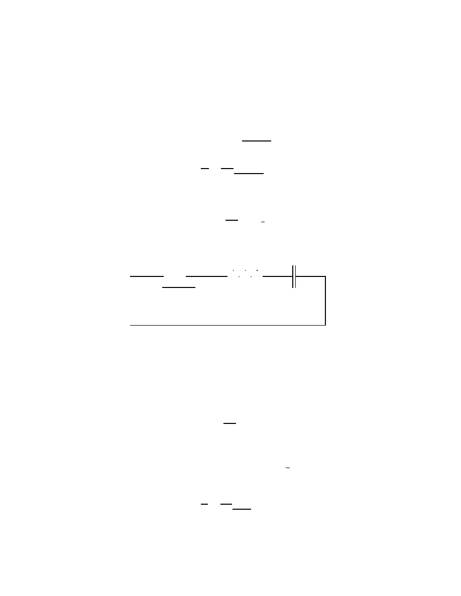
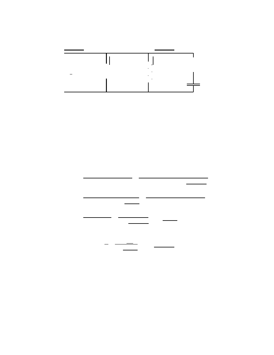
The impedance of the series RLC circuit shown in Fig. 2 is the complex number
Z = R + jωL −
j
ωC
=
|Z|
θ
Ω
(8)
where ω = 2πf is the angular frequency in rad/s, R is the resistance in ohms, L is the
inductance in henrys, and C is the capacitance in farads.
∨ ∨ ∨
∧ ∧ ∧
R
L
C
V
-
I
Figure 2: Series RLC circuit.
We define the reactances of the inductance and capacitance as
X
L
= ωL
Ω
(9)
X
C
=
1
ωC
Ω
(10)
Reactances are always real numbers. The impedance of an inductor, Z = jX
L
, is imaginary,
but X
L
itself (and X
C
) is real and positive.
When a phasor root-mean-square voltage (rms) V = |V |
θ is applied to an impedance,
the resulting phasor rms current is
I =
V
Z
=
|V |
|Z|
/ − θ
A
(11)
Wind Energy Systems by Dr. Gary L. Johnson
November 21, 2001
Chapter 5—Electrical Network
5–7
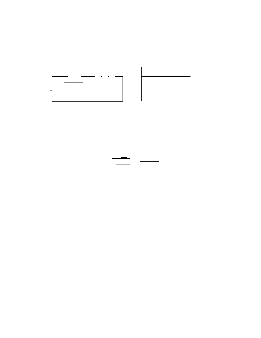
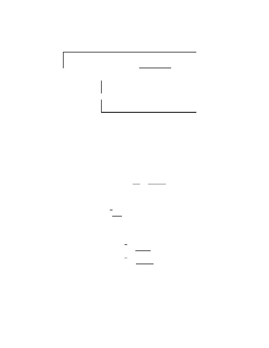
Example
The RL circuit shown in Fig. 3 has R = 6 Ω, X
L
= 8 Ω, and V = 200/0
o
. What is the current?
∨ ∨ ∨
∧ ∧ ∧
6 Ω
j8 Ω
200
0
o
V
-
I
-
6
S
S
S
S
S
S
w
V
I
53.13
o
Figure 3: Series RL Circuit.
First we find the impedance Z.
Z = R + jX
L
= 6 + j8 = 10/53.13
o
The current is then
I =
200/0
o
10/53.13
o
= 20/ − 53.13
o
A sketch of V and I on the complex plane for this example is also shown in Fig. 3. This
sketch is called a phasor diagram. The current in this inductive circuit is said to lag V. In
a capacitive circuit the current will lead V. The words “lead” and “lag” always apply to the
relationship of the current to the voltage. The phrase “ELI the ICE man” is sometimes used
to help beginning students remember these fundamental relationships. The word ELI has
the middle letter L (inductance) with E (voltage) before, and I (current) after or lagging the
voltage. The word ICE has the middle letter C (capacitance) with E after, and I before or
leading the voltage in a capacitive circuit.
In addition to the voltage, current, and impedance of a circuit, we are also interested in
the power. There are three types of power which are considered in ac circuits, the complex
power S, the real power P , and the reactive power Q. The relationship among these quantities
is
S = P + jQ = |S|
θ
VA
(12)
The magnitude of the complex power, called the volt-amperes or the apparent power of the
circuit is defined as
|S| = |V ||I|
VA
(13)
The real power is defined as
Wind Energy Systems by Dr. Gary L. Johnson
November 21, 2001
Chapter 5—Electrical Network
5–8
P = |V ||I| cos θ
W
(14)
The reactive power is defined as
Q = |V ||I| sin θ
var
(15)
The angle θ is the difference between the angle of voltage and the angle of current.
θ = /V − /I
rad
(16)
The power factor is defined as
pf = cos θ = cos
tan
−1
Q
P
(17)
The real power supplied to a resistor is
P = V I = I
2
R =
V
2
R
W
(18)
where V and I are the voltage across and the current through the resistor.
The magnitude of the reactive power supplied to a reactance is
|Q| = V I = I
2
X =
V
2
X
var
(19)
where V and I are the voltage across and the current through the reactance. Q will be
positive to an inductor and negative to a capacitor. The units of reactive power are volt-
amperes reactive or vars.
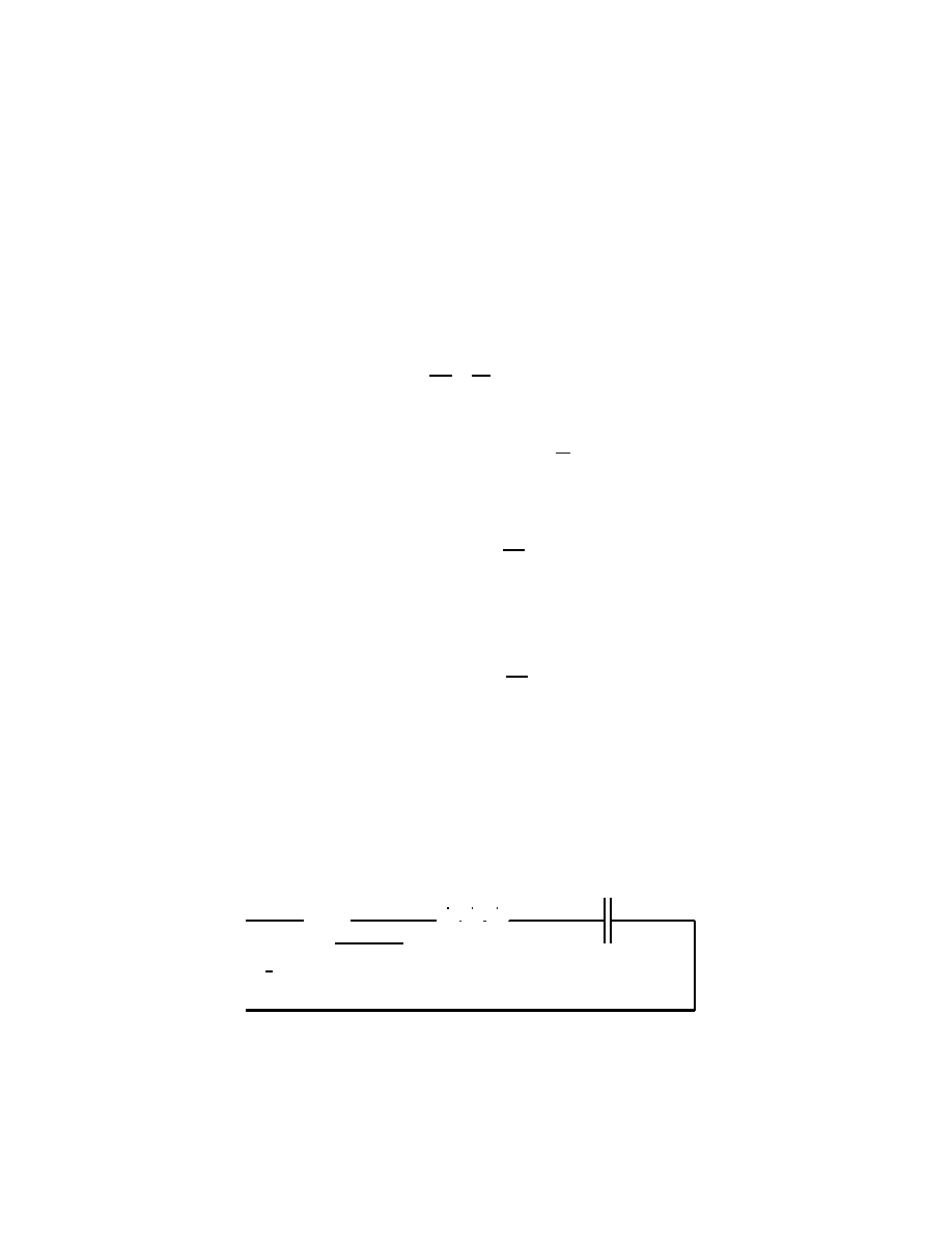
Example
A series RLC circuit, shown in Fig. 4, has R = 4 Ω, X
L
= 8 Ω, and X
C
= 11 Ω. Find the current,
complex power, real power, and reactive power delivered to the circuit for an applied voltage of 100 V.
What is the power factor?
∨ ∨ ∨
∧ ∧ ∧
4 Ω
j8 Ω
−j11 Ω
V = 100
0
o
-
I
Figure 4: Series RLC circuit.
Wind Energy Systems by Dr. Gary L. Johnson
November 21, 2001

Chapter 5—Electrical Network
5–9
The impedance is
Z = R + jX
L
− jX
C
= 4 + j8 − j11 = 4 − j3 = 5/ − 36.87
o
Ω
Assuming V = |V |/0
o
is the reference voltage, the current is
I =
V
Z
=
100/0
o
5/ − 36.87
o
= 20/36.87
o
A
The complex power is
S = |V ||I|
θ = (100)(20)/ − 36.87
o
= 2000/ − 36.87
o
VA
The real power supplied to the circuit is just the real power absorbed by the resistor, since reactances
do not absorb real power.
P = I
2
R = (20)
2
(4) = 1600 W
It is also given by
P = |V ||I| cos θ = 100(20) cos /36.87
o
= 1600 W
The reactive power supplied to the inductor is
Q
L
= I
2
X
L
= (20)
2
(8) = 3200 var
The reactive power supplied to the capacitor is
Q
C
=
−I
2
X
C
=
−(20)
2
(11) =
−4400 var
The net reactive power supplied to the circuit is
Q = Q
L
+ Q
C
= 3200
− 4400 = −1200 var
It is also given by
Q = |V ||I| sin θ = 100(20) sin(−36.87
o
) =
−1200 var
The power factor is
pf = cos θ = cos(−36.87
o
) = 0.8 lead
The word “lead” indicates that θ is negative, or that the current is leading the voltage.
We see that the real and reactive powers can be found either from the input voltage and
current or from the summation of the component real and reactive powers within the circuit.
Wind Energy Systems by Dr. Gary L. Johnson
November 21, 2001
Chapter 5—Electrical Network
5–10
-
-
<
<
<
>
>
>
<
<
<
>
>
>
?
?
V = 100
0
o
I
I
3
I
1
I
2
4 Ω
j8 Ω
6 Ω
−j11 Ω
Figure 5: Parallel RLC circuit.
The effort required may be smaller or greater for one approach as compared to the other,
depending on the structure of the circuit. The student should consider the relative difficulty
of both techniques before solving the problem, to minimize the total effort.
Example
Find the apparent power and power factor of the circuit in Fig. 5.
One solution technique is to first find the input impedance.
Z
=
1
1/4 + 1/j8 + 1/(6 − j11)
=
1
0.25 − j0.125 + 1/(12.53/ − 61.39
o
)
=
1
0.25 − j0.125 + 0.080/61.39
o
=
1
0.25 − j0.125 + 0.038 + j0.070
=
1
0.288 − j0.055
=
1
0.293/ − 10.79
o
= 3.41/10.79
o
Ω
The input current is then
I =
V
Z
=
100/0
o
3.41/10.79
o
= 29.33/ − 10.79
o
A
The apparent power is
|S| = |V ||I| = 100(29.33) = 2933 VA
The power factor is
pf = cos θ = cos 10.79
o
= 0.982 lag
Another solution technique is to find the individual component powers. We have to find the current
I
3
to find the real and reactive powers supplied to that branch.
Wind Energy Systems by Dr. Gary L. Johnson
November 21, 2001

Chapter 5—Electrical Network
5–11
I
3
=
V
6
− j11
=
100/0
o
12.53/ − 61.39
o
= 7.98/61.39
o
The capacitive reactive power is then
Q
C
=
−|I
3
|
2
X
C
=
−(7.98)
2
(11) =
−700 var
The inductive reactive power is
Q
L
=
V
2
X
L
=
(100)
2
8
= 1250 var
The real power supplied to the circuit is
P =
V
2
4
+
|I
3
|
2
(6) =
(100)
2
4
+ (7.98)
2
(6) = 2500 + 382 = 2882 W
The complex power is then
S = P + jQ = 2882 + j1250 − j700 = 2882 + j550 = 2934/10.80
o
var
so the apparent power is 2934 var and the power factor is
pf = cos /10.80
o
= 0.982 lag
The total effort by a person proficient in complex arithmetic may be about the same for either
approach. A beginner is more likely to get the correct result from the second approach, however,
because it reduces the required complex arithmetic by not requiring the determination of the input
impedance.
We now turn our attention to three-phase circuits. We are normally interested in a bal-
anced set of voltages connected in wye as shown in Fig. 6. If we select E
a
, the voltage of point
a with respect to the neutral point n, as the reference, then
E
a
=
|E
a
|/0
o
V
E
b
=
|E
a
|/ − 120
o
V
(20)
E
c
=
|E
a
|/ − 240
o
V
This set of voltages is said to form an abc sequence, since E
b
lags E
a
by 120
o
, and E
c
lags
E
b
by 120
o
. We use the symbol E rather than V to indicate that we have a source voltage.
Wind Energy Systems by Dr. Gary L. Johnson
November 21, 2001
Chapter 5—Electrical Network
5–12
m
m
m
P
P
P
P
PPPP
q
q
q
E
a
E
b
E
c
n
+
+
+
E
bc
E
ab
E
ca
+
−
+
−
+
−
a
b
c
Figure 6: Balanced three-phase source.
The symbol V will be used for other types of voltages in the circuit. This will become more
evident after a few examples.
The line to line voltage E
ab
is given by
E
ab
=
E
a
− E
b
=
|E
a
|(1/0
o
− 1/ − 120
o
)
=
|E
a
|[1 − (−0.5 − j0.866)] = |Ea|(1.5 + j0.866)
=
|Ea|
√
3/30
o
V
(21)
In a similar fashion,
E
bc
=
√
3
|E
a
|/ − 90
o
V
E
ca
=
√
3
|Ea|/ − 210
o
V
(22)
These voltages are shown in the phasor diagram of Fig. 7.
When this three-phase source is connected to a balanced three-phase wye-connected load,
we have the circuit shown in Fig. 8.
The current I
a
is given by
Wind Energy Systems by Dr. Gary L. Johnson
November 21, 2001
Chapter 5—Electrical Network
5–13
*
H
H
H
H
H
H
H
H
H
Y
?
-
A
A
A
A
AAK
E
a
E
ab
E
ca
E
bc
E
b
E
c
Figure 7: Balanced three-phase voltages for circuit in Fig. 5.6.
H
H
H
H
HH
HH
m
m
m
Z
H
H
H
HH
H
H
H
H
H
H
H
A
A
A
A
A
A
Z
Z
-
I
a
-
I
b
-
I
c
I
n
r
r
r
r
a
b
n
c
E
c
E
a
E
b
Figure 8: Balanced three-phase wye-connected source and load.
I
a
=
E
a
Z
=
|E
a
|
|Z|
/ − θ =
|I
a
|/ − θ
A
(23)
The other two currents are given by
I
b
=
|I
a
|/ − θ − 120
o
A
I
c
=
|I
a
|/ − θ − 240
o
A
(24)
The sum of the three currents is the current I
n
flowing in the neutral connection, which can
Wind Energy Systems by Dr. Gary L. Johnson
November 21, 2001

Chapter 5—Electrical Network
5–14
easily be shown to be zero in the balanced case.
I
n
= I
a
+ I
b
+ I
c
= 0 A
(25)
The total power supplied to the load is three times the power supplied to each phase.
|S
tot
| = 3|E
a
||I
a
|
VA
P
tot
=
3
|E
a
||I
a
| cos θ
W
(26)
Q
tot
=
3
|E
a
||I
a
| sin θ
var
The total power can also be expressed in terms of the line-to-line voltage E
ab
.
|S
tot
| =
√
3
|E
ab
||I
a
|
VA
P
tot
=
√
3
|E
ab
||I
a
| cos θ
W
(27)
Q
tot
=
√
3
|E
ab
||I
a
| sin θ
var
We shall illustrate the use of these equations in the discussion on synchronous generators
in the next section.
3 THE SYNCHRONOUS GENERATOR
Almost all electrical power is generated by three-phase ac generators which are synchronized
with the utility grid. Engine driven single-phase generators are used sometimes, primarily for
emergency purposes in sizes up to about 50 kW. Single-phase generators would be used for
wind turbines only when power requirements are small (less than perhaps 20 kW) and when
utility service is only single-phase. A three-phase machine would normally be used whenever
the wind turbine is adjacent to a three-phase transmission or distribution line. Three-phase
machines tend to be smaller, less expensive, and more efficient than single-phase machines of
the same power rating, which explains their use whenever possible.
It is beyond the scope of this text to present a complete treatment of three-phase syn-
chronous generators. This is done by many texts on electrical machines. A brief overview is
necessary, however, before some of the important features of ac generators connected to wind
turbines can be properly discussed.
Wind Energy Systems by Dr. Gary L. Johnson
November 21, 2001
Chapter 5—Electrical Network
5–15
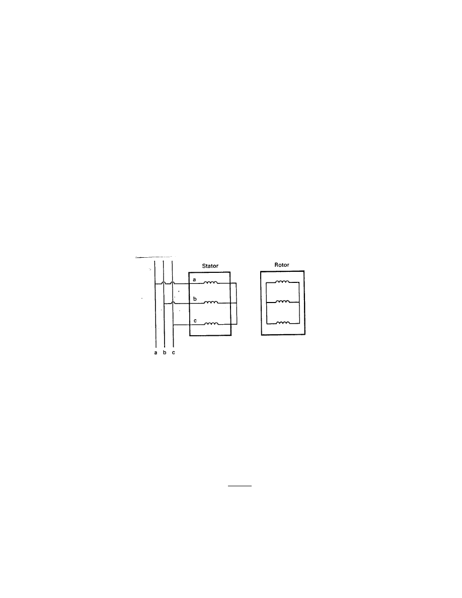
A construction diagram of a three-phase ac generator is shown in Fig. 9. There is a rotor
which is supplied a direct current I
f
through slip rings. The current I
f
produces a flux Φ.
This flux couples into three identical coils, marked aa
, bb
, and cc
, spaced 120
o
apart, and
produces three voltage waveforms of the same magnitude but 120 electrical degrees apart.
...............
................
................
.................
.................
..................
....................
.......................
............................
.........................................
.........................................................................................................
....................
................
..............
.............
............
...........
..........
..........
.........
..........
.........
.........
.........
.........
.........
.........
.........
........
........
.........
........
.........
.........
.........
.........
........
........
.......
.......
......
......
.....
......
.....
.....
.....
.....
.....
.....
.....
.....
....
....
....
....
....
....
....
....
....
....
....
....
....
....
....
....
....
....
....
....
....
....
....
....
....
....
....
....
....
....
....
....
....
....
....
....
....
....
....
.....
....
.....
.....
.....
.....
.....
.....
......
......
.......
.......
........
..........
...........
..................
.................
.................
................
................
...............
.......
...............
................
.................
..................
...................
......................
............................
................................................................................................................................
...............
.............
............
...........
..........
..........
..........
.........
.........
.........
.........
.........
........
........
.........
.........
.........
.........
.........
........
.......
......
......
......
.....
.....
.....
.....
.....
....
.....
....
....
....
....
....
....
....
....
....
....
....
....
....
....
....
....
....
....
....
....
....
....
....
....
....
....
....
....
....
....
....
.....
.....
.....
.....
.....
.....
.....
.......
.......
........
..........
.................
..................
.................
................
...............
....
....
....
....
....
....
....
....
....
....
....
....
....
....
....
....
....
....
....
....
....
....
....
....
....
....
.....
.....
...
.................................................................................................................
........
.........
.........
.........
.........
........
.....
∨
ω
k
k
k
k
k
k
6
Φ
-
I
f
s
Figure 9: Three-phase generator
The equivalent circuit for one phase of this ac generator is shown in Fig. 10. It is shown in
electrical machinery texts that the magnitude of the generated rms electromotive force (emf)
E is given by
|E| = k
1
ωΦ
(28)
where ω = 2πf is the electrical radian frequency, Φ is the flux per pole, and k
1
is a constant
which includes the number of poles and the number of turns in each winding. The reactance X
s
is the synchronous reactance of the generator in ohms/phase. The generator reactance changes
from steady-state to transient operation, and X
s
is the steady-state value. The resistance R
s
represents the resistance of the conductors in the generator windings. It is normally much
smaller than X
s
, so is normally neglected except in efficiency calculations. The synchronous
impedance of the winding is given the symbol Z
s
= R
s
+ jX
s
.
The voltage E is the open circuit voltage and is sometimes called the voltage behind
synchronous reactance. It is the same as the voltage E
a
of Fig. 8.
The three coils of the generator can be connected together in either wye or delta, although
the wye connection shown in Fig. 8 is much more common. When connected in wye, E is the
line to neutral voltage and one has to multiply it by
√
3 to get the magnitude of the line-to-line
voltage.
The frequency f of the generated emf is given by
Wind Energy Systems by Dr. Gary L. Johnson
November 21, 2001

Chapter 5—Electrical Network
5–16
m
∨ ∨ ∨
∧ ∧ ∧
-
I
jX
s
R
s
E
V
∆V
+
−
+
+
−
Figure 10: Equivalent circuit for one phase of a synchronous three-phase generator.
f =
p
2
n
60
Hz
(29)
where p is the number of poles and n is the rotational speed in r/min. The speed required
to produce 60 Hz is 3600 r/min for a two pole machine, 1800 r/min for a four pole machine,
1200 r/min for a six pole machine, and so on. It is possible to build generators with large
numbers of poles where slow speed operation is desired. A hydroelectric plant might use a
72 pole generator, for example, which would rotate at 100 r/min to produce 60 Hz power.
A slow speed generator could be connected directly to a wind turbine, eliminating the need
for an intermediate gearbox. The propellers of the larger wind turbines turn at 40 r/min or
less, so a rather large number of poles would be required in the generator for a gearbox to be
completely eliminated. Both cost and size of the generator increase with the number of poles,
so the system cost with a very low speed generator and no gearbox may be greater than the
cost for a higher speed generator and a gearbox.
When the generator is connected to a utility grid, both the grid or terminal voltage V
and the frequency f are fixed. The machine emf E may differ from V in both magnitude and
phase, so there exists a difference voltage
∆V = E − V
V/phase
(30)
This difference voltage will yield a line current I (defined positive away from the machine)
of value
I =
∆V
Z
s
A
(31)
The relationship among E, V , and I is shown in the phasor diagram of Fig. 11. E is
proportional to the rotor flux Φ which in turn is proportional to the field current flowing in
the rotor. When the field current is relatively small, E will be less than V . This is called the
underexcitation case. The case where E is greater than V is called overexcitation. E will lead
V by an angle δ while I will lag or lead V by an angle θ.
The conventions for the angles θ and δ are
Wind Energy Systems by Dr. Gary L. Johnson
November 21, 2001
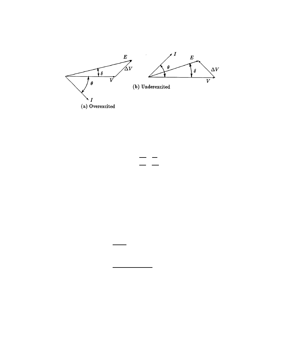
Chapter 5—Electrical Network
5–17
Figure 11: Phasor diagram of one phase of a synchronous three-phase generator: (a) overex-
cited; (b) underexcited.
θ = /V
− /I
δ = /E − /V
(32)
Phasors in the first quadrant have positive angles while phasors in the fourth quadrant have
negative angles. Therefore, both θ and δ are positive in the overexcited case, while δ is positive
and θ is negative in the underexcited case.
Expressions for the real and reactive powers supplied by each phase were given in Eqs. 14
and 15 in terms of the terminal voltage V and the angle θ. We can apply some trigonometric
identities to the phasor diagrams of Fig. 11 and arrive at alternative expressions for P and Q
in terms of E, V , and the angle δ.
P
=
|E||V |
X
s
sin δ
W/phase
Q =
|E||V | cos δ − |V |
2
X
s
var/phase
(33)
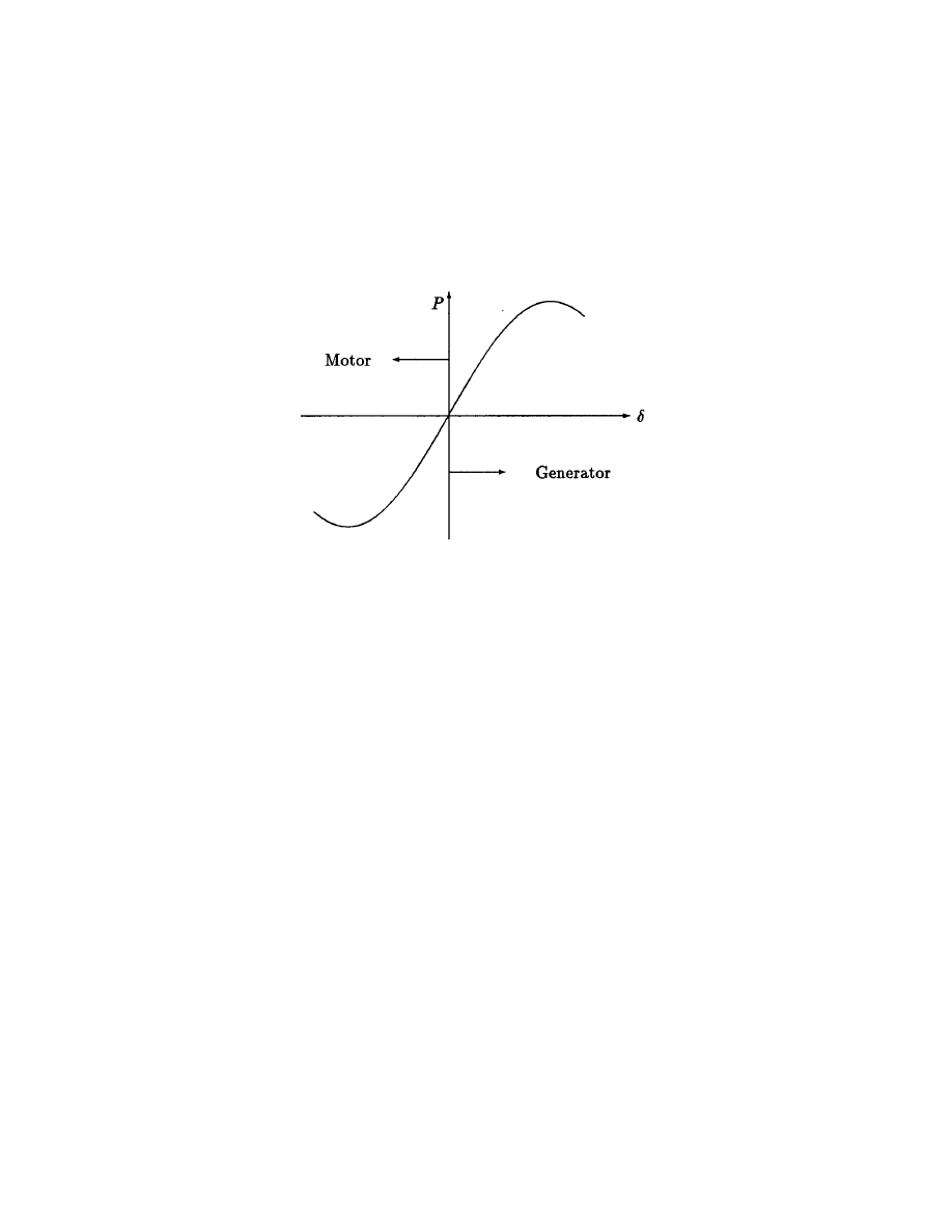
A plot of P versus δ is shown in Fig. 12. This illustrates two important points about
the use of an ac generator. One is that as the input mechanical power increases, the output
electrical power will increase, reaching a maximum at δ = 90
o
. This maximum electrical
power, occurring at sin δ = 1, is called the pullout power. If the input mechanical power
is increased still more, the output power will begin to decrease, causing a rapid increase in
δ and a loss of synchronism. If a turbine is operating near rated power, and a sharp gust
Wind Energy Systems by Dr. Gary L. Johnson
November 21, 2001
Chapter 5—Electrical Network
5–18
of wind causes the input power to exceed the pullout power from the generator, the rotor
will accelerate above rated speed. Large generator currents will flow and the generator will
have to be switched off the power line. Then the rotor will have to be slowed down and the
generator resynchronized with the grid. Rapid pitch control of the rotor can prevent this, but
the control system will have to be well designed.
Figure 12: Power flow from an ac generator as a function of power angle.
The other feature illustrated by this power plot is that the power becomes negative for
negative δ. This means the generator is now acting as a motor. Power is being taken from the
electric utility to operate a giant fan and speed up the air passing through the turbine. This
is not the purpose of the system, so when the wind speed drops below some critical value, the
generator must be disconnected from the utility line to prevent motoring.
Before working an example, we need to discuss generator rating. Generators are often
rated in terms of apparent power rather than real power. The reason for this is the fact that
generator losses and the need for generator cooling are not directly proportional to the real
power. The generator will have hysteresis and eddy current losses which are determined by
the voltage, and ohmic losses which are determined by the current. The generator can be
operated at rated voltage and rated current, and therefore with rated losses, even when the
real power is zero because θ = 90 degrees. A generator may be operated at power factors
between 1.0 and 0.7 or even lower depending on the requirements of the grid, so the product
of rated voltage and rated current (the rated apparent power) is a better measure of generator
capability than real power. The same argument is true for transformers, which always have
their ratings specified in kVA or MVA rather than kW or MW.
A generator may also have a real power rating which is determined by the allowable torque
in the generator shaft. A rating of 2500 kVA and 2000 kW, or 2500 kVA at 0.8 power factor,
would imply that the machine is designed for continuous operation at 2500 kVA output, with
2000 kW plus losses being delivered to the generator through its shaft. There are always safety
Wind Energy Systems by Dr. Gary L. Johnson
November 21, 2001

Chapter 5—Electrical Network
5–19
factors built into the design for short term overloads, but one should not plan to operate a
generator above its rated apparent power or above its rated real power for long periods of
time.
We should also note that generators are rarely operated at exactly rated values. A gen-
erator rated at 220 V and 30 A may be operated at 240 V and 20 A, for example. The
power in the wind is continuously varying, so a generator rated at 2500 kVA and 2000 kW
may be delivering 300 kW to the grid one minute and 600 kW the next minute. Even when
the source is controllable, as in a coal-fired generating plant, a 700-MW generator may be
operated at 400 MW because of low demand. It is therefore important to distinguish between
rated conditions and operating conditions in any calculations.
Rated conditions may not be completely specified on the equipment nameplate, in which
case some computation is required. If a generator has a per phase rated apparent power S
R
and a rated line to neutral voltage V
R
, the rated current is
I
R
=
S
R
V
R
(34)
Example
The MOD-0 wind turbine has an 1800 r/min synchronous generator rated at 125 kVA at 0.8 pf and
480 volts line to line[8]. The generator parameters are R
s
= 0.033 Ω/phase and X
s
= 4.073 Ω/phase.
The generator is delivering 75 kW to the grid at rated voltage and 0.85 power factor lagging. Find
the rated current, the phasor operating current, the total reactive power, the line to neutral phasor
generated voltage E, the power angle delta, the three-phase ohmic losses in the stator, and the pullout
power.
The first step in the solution is to determine the per phase value of terminal voltage, which is
|V | =
480
√
3
= 277 V/phase
The rated apparent power per phase is
S
R
=
125
3
= 41.67 kVA/phase = 41, 670 VA/phase
The rated current is then
I
R
=
S
R
V
R
=
41, 670
277
= 150.4 A
The real power being supplied to the grid per phase is
P =
75
3
= 25 kW/phase = 25 × 10
3
W/phase
From Eq. 14 we can find the magnitude of the phasor operating current to be
Wind Energy Systems by Dr. Gary L. Johnson
November 21, 2001

Chapter 5—Electrical Network
5–20
|I| =
P
|V | cos θ
=
25
× 10
3
277(0.85)
= 106.2 A
The angle θ is
θ = cos
−1
(0.85) = +31.79
o
The phasor operating current is then
I = |I|/ − θ = 106.2/ − 31.79
o
= 90.3 − j55.9 A
The reactive power supplied per phase is
Q = (277)(106.2) sin 31.79
o
= 15, 500 var/phase
The generator is then supplying a total reactive power of 46.5 kvar to the grid in addition to the total
real power of 75 kW.
The voltage E is given by Kirchhoff’s voltage law.
E = V + IZ
s
=
277/0
o
+ 106.2/ − 31.79
o
(0.033 + j4.073)
=
508 + j366 = 626/35.77
o
V/phase
Since the terminal voltage V has been taken as the reference (V = |V |/0
o
), the power angle is just the
angle of E, or 35.77
o
. The total stator ohmic loss is
P
loss
= 3I
2
R
s
= 3(106.2)
2
(0.033) = 1.117 kW
This is a small fraction of the total power being delivered to the utility, but still represents a significant
amount of heat which must be transferred to the atmosphere by the generator cooling system.
The pullout power, given by Eq. 33 with sin δ = 1 is
P =
|E||V |
X
s
=
626(277)
4.073
= 42.6 kW/phase
or a total of 128 kW for the total machine. As mentioned earlier, if the input shaft power would rise
above the pullout power from a wind gust, the generator would lose synchronism with the power grid.
In most systems, the pullout power will be at least twice the rated power of the generator to prevent
this possibility. This larger pullout power represents a somewhat better safety margin than is available
in the MOD-0 system.
One advantage of the synchronous generator is its ability to supply either inductive or
capacitive reactive power to a load. The generated voltage
|E| is produced by a current
Wind Energy Systems by Dr. Gary L. Johnson
November 21, 2001
Chapter 5—Electrical Network
5–21
flowing in the field winding, which is controlled by a control system. If the field current is
increased, then
|E| must increase. If the real power is fixed by the prime mover, then from
Eq. 33 we see that sin δ must decrease by a proportional amount as |E| increases. This causes
the reactive power flow to increase. A decrease in
|E| will cause Q to decrease, eventually
becoming negative. A synchronous generator rated at 125 kVA and 0.8 power factor can
supply its rated real power of 100 kW and at the same time can supply any value of reactive
power between +75 kvar and
−75 kvar to the grid. Most loads require some reactive power
for operation, so the synchronous generator can meet all the requirements of a load while
requiring nothing from the load. It can operate in an independent mode as well as intertied
with a utility grid.
The major disadvantage of a synchronous generator is its complexity and cost, as well as the
cost of the required control systems. Some of the complexity is shown by the synchronization
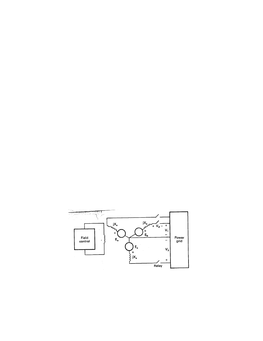
process, as illustrated in Fig. 13. From a complete stop, the first step is to start the rotor.
The sensors will measure wind direction and actuate the direction controls so the turbine is
properly directed into the wind. If the wind speed is above the cut-in value, the pitch controls
will change the propeller pitch so rotation can occur. The generator field control is activated
so a predetermined current is sent through the field of the generator. A fixed field current
fixes the flux Φ, so that E is proportional to the rotational speed n. The turbine accelerates
until it almost reaches rated angular velocity. At this point the frequency of E will be about
the same as that of the power grid. The amplitude of E will be about the same as V if the
generator field current is correct. Slightly different frequencies will cause the phase difference
between E and V to change slowly over the range of 0 to 360
o
. The voltage difference V
d
is
sensed so the relay can be closed when V
d
is a minimum. This limits the transient current
through the relay contacts, thus prolonging their lives, and also minimizes the shock to both
the generator and the power grid. If the relay is closed when V
d
is not close to its minimum,
very high currents will flow until the generator is accelerated or decelerated to the rotational
position where E and V are in phase.
Figure 13: AC generator being synchronized with the power grid.
Once the relay is closed, there will still be no power flow as long as E and V have the same
Wind Energy Systems by Dr. Gary L. Johnson
November 21, 2001

Chapter 5—Electrical Network
5–22
magnitude and phase. Generator action is obtained by increasing the magnitude of E with
the field control. The pitch controller sets the blade pitch at the optimum point if the blades
are not already at this point. The blade torque will attempt to accelerate the generator, but
this is impossible because the generator and the power grid are in synchronism. The torque
will advance the relative position of the generator rotor with respect to the power grid voltage,
however, so E will lead V by the power angle δ. The input mechanical power to the generator
is fixed for a given wind speed and blade pitch, which also fixes the output power. If
|E|
is changed by the generator field control, then the power angle will change automatically to
maintain this fixed output power.
This synchronization process may sound very difficult, but is accomplished routinely by
automatic equipment.
If the wind speed and blade pitch are such that the turbine and
generator are slowly accelerating through synchronous speed, the relay can usually be closed
just as synchronous speed is reached. The microprocessor control would then adjust the field
current and the blade pitch for proper operating conditions. An observer would see a smooth
operation lasting only a minute or so.
The control systems necessary for synchronization and the generator field supply are not
cheap. On the other hand, their costs are not strongly dependent on system size over the
normal range of wind turbine sizes. This means that the control systems would form a small
fraction of the total turbine cost for a 1000-kW turbine, but a substantial fraction for a 5-kW
turbine. For this reason, the synchronous generator will be more common in sizes of 100 kW
and up, and not so common in the smaller sizes.
4 PER UNIT CALCULATIONS
Problems such as those in the previous section can always be worked using the actual circuit
values. There is an alternative, however, to the use of actual circuit values which has several
advantages and which is widely used in the electric power industry. This is the per unit system,
in which voltages, currents, powers, and impedances are all expressed as a percent or per unit
of a base or reference value. For example, if a base voltage of 120 V is chosen, voltages of 108,
120, and 126 V become 0.90, 1.00, and 1.05 per unit, or 90, 100, and 105 percent, respectively.
The per unit value of any quantity is defined as the ratio of the quantity to its base value,
expressed as a decimal.
One advantage of the per unit system is that the product of two quantities expressed in per
unit is also in per unit. Another advantage is that the per unit impedance of an ac generator
is essentially a constant for a wide range of actual sizes. This means that a problem like the
preceding example needs to be worked only once in per unit, with the results converted to
actual values for each particular size of machine for which results are needed.
We shall choose the base or reference as the per phase quantities of a three-phase system.
The base radian frequency ω
base
= ω
o
is the rated radian frequency of the system, normally
Wind Energy Systems by Dr. Gary L. Johnson
November 21, 2001
Chapter 5—Electrical Network
5–23
2π(60) = 377 rad/s.
Given the base apparent power per phase S
base
and base line to neutral voltage V
base
, the
following relationships are valid:
I
base
=
S
base
V base
A
(35)
Z
base
= R
base
= X
base
=
V
base
I
base
Ω
(36)
P
base
= Q
base
= S
base
VA
(37)
We may even define a base inductance and a base capacitance.
L
base
=
X
base
ω
o
(38)
C
base
=
1
X
base
ω
o
(39)
The per unit values are then the actual values divided by the base values.
V
pu
=
V
V
base
(40)
I
pu
=
I
Ibase
(41)
Z
pu
=
Z
Zbase
(42)
ω
pu
=
ω
ω
base
=
ω
ω
o
(43)
L
pu
=
L
L
base
(44)
C
pu
=
C
C
base
(45)
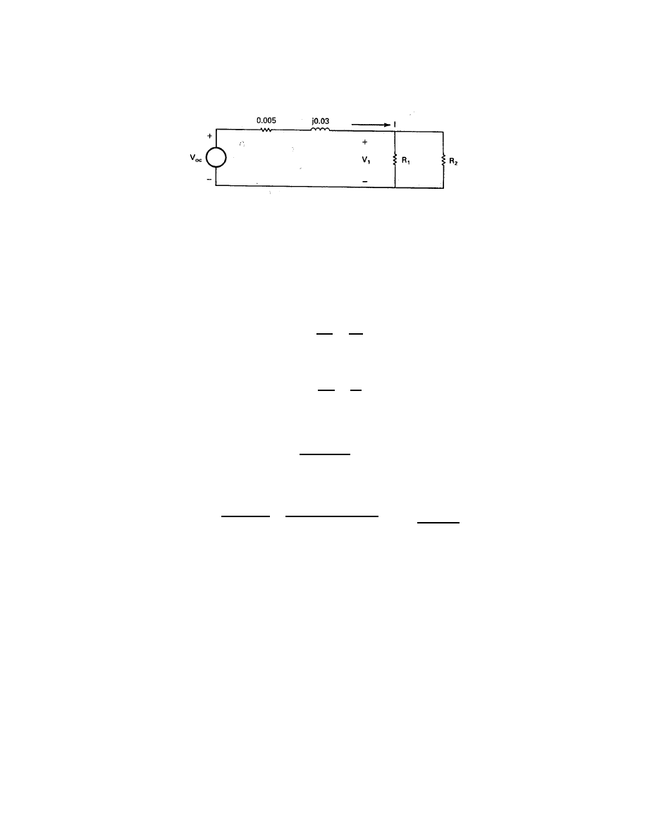
Example
Wind Energy Systems by Dr. Gary L. Johnson
November 21, 2001
Chapter 5—Electrical Network
5–24
The MOD-2 generator is rated at 3125 kVA, 0.8 pf, and 4160 V line to line. The typical per phase
synchronous reactance for the four-pole, conventionally cooled generator is 1.38 pu. The generator is
supplying power at rated voltage and frequency to an isolated load with a per phase impedance of
1.2 - j0.8 pu as shown in Fig. 14. Find the base, actual, and per unit values of terminal voltage V ,
generated voltage E, apparent power, real power, reactive power, current, generator inductance, and
load capacitance.
m
<
<
<
>
>
>
E
j1.38 pu
1.2 pu
−j0.8 pu
V
+
−
+
−
Figure 14: Per phase diagram for example problem.
First we determine the base values, which do not depend on actual operating conditions but on
nameplate ratings.
V
base
=
4160
√
3
= 2400 V
E
base
= V
base
= 2400 V
S
base
=
3125
3
= 1042 kVA
P
base
= Q
base
= S
base
= 1042 kVA
I
base
=
S
base
V
base
=
1, 042, 000 VA
2400 V
= 434 A
Z
base
=
V
base
I
base
=
2400
434
= 5.53 Ω
L
base
=
X
base
ω
o
=
Z
base
ω
o
=
5.53
377
= 14.7 mH
C
base
=
1
X
base
ω
o
=
1
5.53(377)
= 480 µF
Wind Energy Systems by Dr. Gary L. Johnson
November 21, 2001
Chapter 5—Electrical Network
5–25
The actual voltage is given in the problem as the rated or base voltage, so
V = 2400 V
The per unit terminal voltage is then
V
pu
=
V
V
base
=
2400
2400
= 1
We now have to solve for the per unit current.
I
pu
=
V
pu
Z
pu
=
1/0
o
1.2 − j0.8
=
1/0
o
1.44/ − 33.69
o
= 0.693/33.69
o
=
0.577 + j0.384
The actual current is
I = I
pu
I
base
= (0.693/33.69
o
)(434) = 300/33.69
o
A
The per unit apparent power is
S
pu
=
|V
pu
||I
pu
| = (1)(0.693) = 0.693
The per unit real power is
P
pu
=
|V
pu
||I
pu
| cos θ = (1)(0.693) cos(−33.69
o
) = 0.577
The per unit reactive power is
Q
pu
=
|V
pu
||I
pu
| sin θ = (1)(0.693) sin(−33.69
o
) =
−0.384
The actual powers per phase are
S
=
(0.693)(1042) = 722 kVA/phase
P
=
(0.577)(1042) = 600 kW/phase
Q = (−0.384)(1042) = −400 kvar/phase
The total power delivered to the three-phase load would then be 2166 kVA, 1800 kW, and -1200 kvar.
The generated voltage E in per unit is
Wind Energy Systems by Dr. Gary L. Johnson
November 21, 2001
Chapter 5—Electrical Network
5–26
E
pu
=
V
pu
+ I
pu
(jX
s,
pu
) = 1 + 0.693/33.69
o
(1.38)/90
o
=
1 + 0.956/123.69
o
= 1
− 0.530 + j0.796
=
0.470 + j0.796 = 0.924/59.46
o
The per unit generator inductance per phase is
L
pu
=
X
s,
pu
ω
pu
=
1.38
1
= 1.38
The actual generator inductance per phase is
L = L
pu
L
base
= 1.38(14.7) = 20.3 mH
The per unit load capacitance per phase is
C
pu
=
1
X
C,
pu
ω
pu
=
1
0.8(1)
= 1.25
The actual load capacitance per phase is
C = C
pu
C
base
= 1.25(480) = 600 µF
The base of any device such as an electrical generator, motor, or transformer is always
understood to be the nameplate rating of the device. The per unit impedance is usually
available from the manufacturer.
Sometimes the base values need to be changed to a common base when several devices are
connected together. Solving an electrical circuit requires either the actual impedances or the
per unit impedances referred to a common base. The per unit impedance on the old base can
be converted to the per unit impedance for the new base by
Z
pu,new
= Z
pu,old
V
base,old
V
base,new
2
S
base,new
S
base,old
(46)
Example
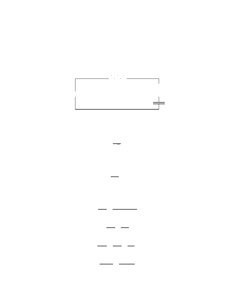
A single-phase distribution transformer secondary is rated at 60 Hz, 10 kVA, and 240 V. The open
circuit voltage V
oc
is 240 V. The per unit series impedance of the transformer is Z = 0.005 + j0.03.
Two electric heaters, one rated 1500 W and 230 V, and the other rated at 1000 W and 220 V, are
connected to the transformer. Find the per unit transformer current I
pu
and the magnitude of the
actual load voltage V
1
, as shown in Fig. 15.
Wind Energy Systems by Dr. Gary L. Johnson
November 21, 2001
Chapter 5—Electrical Network
5–27
Figure 15: Single-phase transformer connected to two resistive loads.
The first step is to get all impedance values computed on the same base. Any choice of base will
work, but minimum effort will be exerted if we choose the transformer base as the reference base. This
yields V
base
= 240 V and S
base
= 10 kVA. The per unit values of the electric heater resistances would
be unity on their nameplate ratings. The per unit values referred to the transformer rating would be
R
1,pu
= (1)
230
240
2
10
1.5
= 6.12
R
2,pu
= (1)
220
240
2
10
1
= 8.40
The equivalent impedance of these heaters in parallel would be
R
pu
=
6.12(8.40)
6.12 + 8.40
= 3.54
The per unit current is then
I
pu
=
V
oc,pu
Z
pu
+ R
pu
=
1
0.005 + j0.03 + 3.54
= 0.282/ − 0.48
o
The load voltage magnitude is
|V
1
| = I
pu
R
pu
V
base
= 0.282(3.54)(240) = 239.6 V
The voltage V
1
has decreased only 0.4 V from the open circuit value for a current of 28.2 percent
of rated. This indicates the voltage varies very little with load changes, which is quite desirable for
transformer outputs.
5 THE INDUCTION MACHINE
A large fraction of all electrical power is consumed by induction motors. For power inputs of
less than 5 kW, these may be either single-phase or three-phase, while the larger machines are
Wind Energy Systems by Dr. Gary L. Johnson
November 21, 2001
Chapter 5—Electrical Network
5–28
almost invariably designed for three-phase operation. Three- phase machines produce a con-
stant torque, as opposed to the pulsating torque of a single-phase machine. They also produce
more power per unit mass of materials than the single-phase machine. The three-phase motor
is a very rugged piece of equipment, often lasting for 50 years with only an occasional change
of bearings. It is simple to construct, and with mass production is relatively inexpensive.
The same machine will operate as either a motor or a generator with no modifications, which
allows us to have a rugged, inexpensive generator on a wind turbine with rather simple control
systems.
The basic wiring diagram for a three-phase induction motor is shown in Fig. 16. The motor
consists of two main parts, the stator or stationary part and the rotor. The most common
type of rotor is the squirrel cage, where aluminum or copper bars are formed in longitudinal
slots in the iron rotor and are short circuited by a conducting ring at each end of the rotor.
The construction is very similar to a three-phase transformer with the secondary shorted, and
the same circuit models apply. In operation, the currents flowing in the three stator windings
produce a rotating flux. This flux induces voltages and currents in the rotor windings. The
flux then interacts with the rotor currents to produce a torque in the direction of flux rotation.
Figure 16: Wiring diagram for a three-phase induction motor.
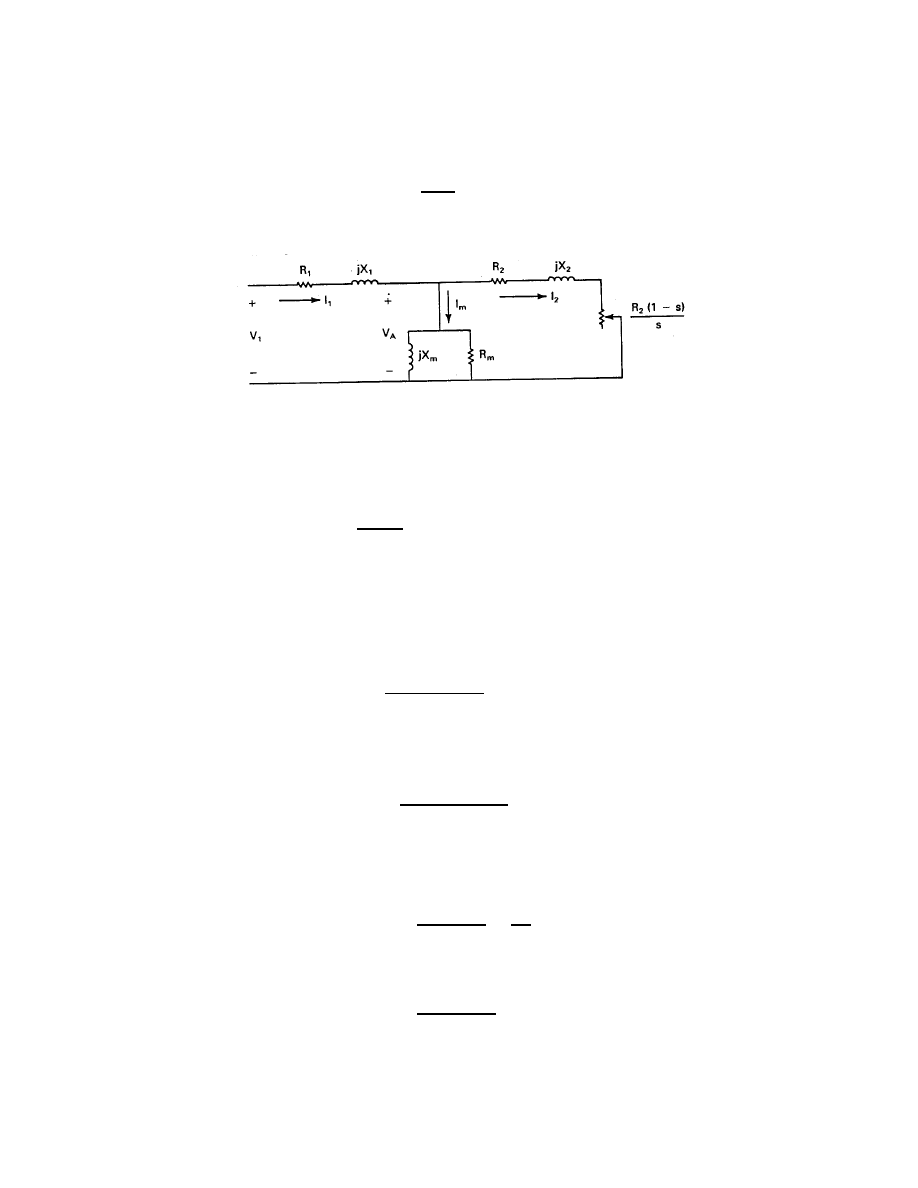
The equivalent circuit of one phase of an induction motor is given in Fig. 17. In this circuit,
R
m
is an equivalent resistance which represents the losses due to eddy currents, hysteresis,
windage, and friction, X
m
is the magnetizing reactance, R
1
is the stator resistance, R
2
is the
rotor resistance, X
1
is the leakage reactance of the stator, X
2
is the leakage reactance of the
rotor, and s is the slip. All resistance and reactance values are referred to the stator. The
reactances X
1
and X
2
are difficult to separate experimentally and are normally assumed equal
to each other. The slip may be defined as
s =
n
s
− n
n
s
(47)
where n
s
is the synchronous rotational speed and n is the actual rotational speed. If the
synchronous frequency is 60 Hz, then from Eq. 29 the synchronous rotational speed will be
Wind Energy Systems by Dr. Gary L. Johnson
November 21, 2001
Chapter 5—Electrical Network
5–29
n
s
=
7200
p
r/min
(48)
where p is the number of poles.
Figure 17: Equivalent circuit for one phase of a three-phase induction motor
The total losses in the motor are given by
P
loss
=
3
|V
A
|
2
R
m
+ 3
|I
1
|
2
R
1
+ 3
|I
2
|
2
R
2
W
(49)
The first term is the loss due to eddy currents, hysteresis, windage, and friction. The second
term is the winding loss (copper loss) in the stator conductors and the third term is the
winding loss in the rotor. The factor of 3 is necessary because of the three phases.
The power delivered to the resistance at the right end of Fig. 17 is
P
m,1
=
|I
2
|
2
R
2
(1
− s)
s
W/phase
(50)
The power P
m,1
is not actually dissipated as heat inside the motor but is delivered to a load
as mechanical power. The total three-phase power delivered to this load is
P
m
=
3
|I
2
|
2
R
2
(1
− s)
s
W
(51)
To analyze the circuit in Fig. 17, we first need to find the impedance Z
in
which is seen by
the voltage V
1
. We can define the impedance of the right hand branch as
Z
2
= R
2
+ jX
2
+
R
2
(1
− s)
s
=
R
2
s
+ jX
2
Ω
(52)
The impedance of the shunt branch is
Z
m
=
jX
m
R
m
R
m
+ jX
m
Ω
(53)
Wind Energy Systems by Dr. Gary L. Johnson
November 21, 2001

Chapter 5—Electrical Network
5–30
The input impedance is then
Z
in
= R
1
+ jX
1
+
Z
m
Z
2
Z
m
+ Z
2
Ω
(54)
The input current is
I
1
=
V
1
Z
in
A
(55)
The voltage across the shunt branch is
V
A
= V
1
− I
1
(R
1
+ jX
1
)
V
(56)
The shunt current I
m
is given by
I
m
=
V
A
Z
m
A
(57)
The current I
2
is given by
I
2
=
V
A
Z
2
A
(58)
The motor efficiency η
m
is defined as the ratio of output power to input power.
η
m
=
P
m
P
m
+ P
loss
(59)
The relationship between motor power P
m
and motor torque T
m
is
P
m
= ω
m
T
m
W
(60)
where
ω
m
=
2πn
60
=
π
30
(1
− s)n
s
rad/s
(61)
By combining the last three equations we obtain the total motor torque
T
m
=
90
|I
2
|
2
R
2
πn
s
s
N
· m/rad
(62)
A typical plot of motor torque versus angular velocity appears in Fig. 18. Also shown
is a possible variation of load torque T
mL
. At start, while n = 0, T
m
will be greater than
T
mL
, allowing the motor to accelerate. As n increases, T
m
increases to a maximum and then
Wind Energy Systems by Dr. Gary L. Johnson
November 21, 2001
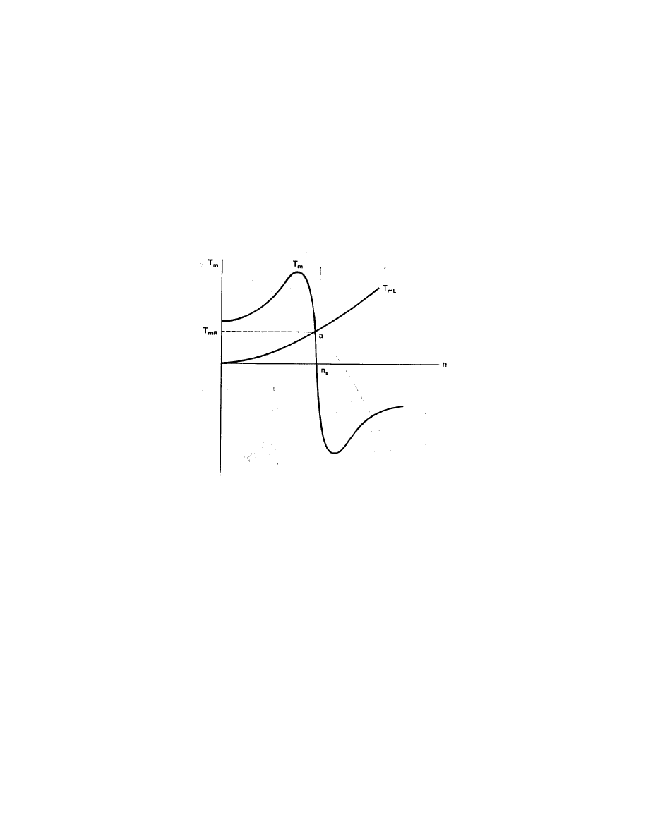
Chapter 5—Electrical Network
5–31
declines rather rapidly toward zero at n = n
s
. Meanwhile the torque required by the load
is increasing with speed. The two torques are equal and steady state operation is reached
at point a in Fig. 18. Rated torque is usually reached at a speed about 3 percent less than
synchronous speed. A four pole induction motor will therefore deliver rated torque at about
1740 r/min, as compared with the synchronous speed of 1800 r/min. The no load speed will
be less than synchronous speed by a few revolutions per minute. The reason for this is that
at synchronous speed the rotor conductors turn in unison with the stator field, which means
there is no time changing magnetic field passing through these conductors to induce a voltage.
Without a voltage there will be no rotor current I
2
, and there is no torque without a current.
Figure 18: Variation of shaft torque with speed for a three-phase induction machine.
If synchronous speed is exceeded, s, T
m
, and P
m
all become negative, indicating that the
mechanical load has become a prime mover and the motor is now acting as a generator. This
means that an induction machine can be connected across a three-phase line, used as a motor
to start a wind turbine such as a Darrieus, and become a generator when the wind starts
to turn the Darrieus. The Darrieus has no pitch control, the induction machine has no field
control, and synchronization is unnecessary, so equipment costs are significantly reduced from
those of the system using a synchronous generator.
The circuit of the induction generator is identical to that of the induction motor, except
that we sometimes draw it reversed, with reversed conventions for I
1
and I
2
as shown in
Fig. 19. The resistance R
2
(1
− s)/s is negative for negative slip, and this negative resistance
can be thought of as a source of power.
The induction generator requires reactive power for excitation. It cannot operate without
this reactive power, so when the connection to the utility is broken in Fig. 19, the induction
Wind Energy Systems by Dr. Gary L. Johnson
November 21, 2001
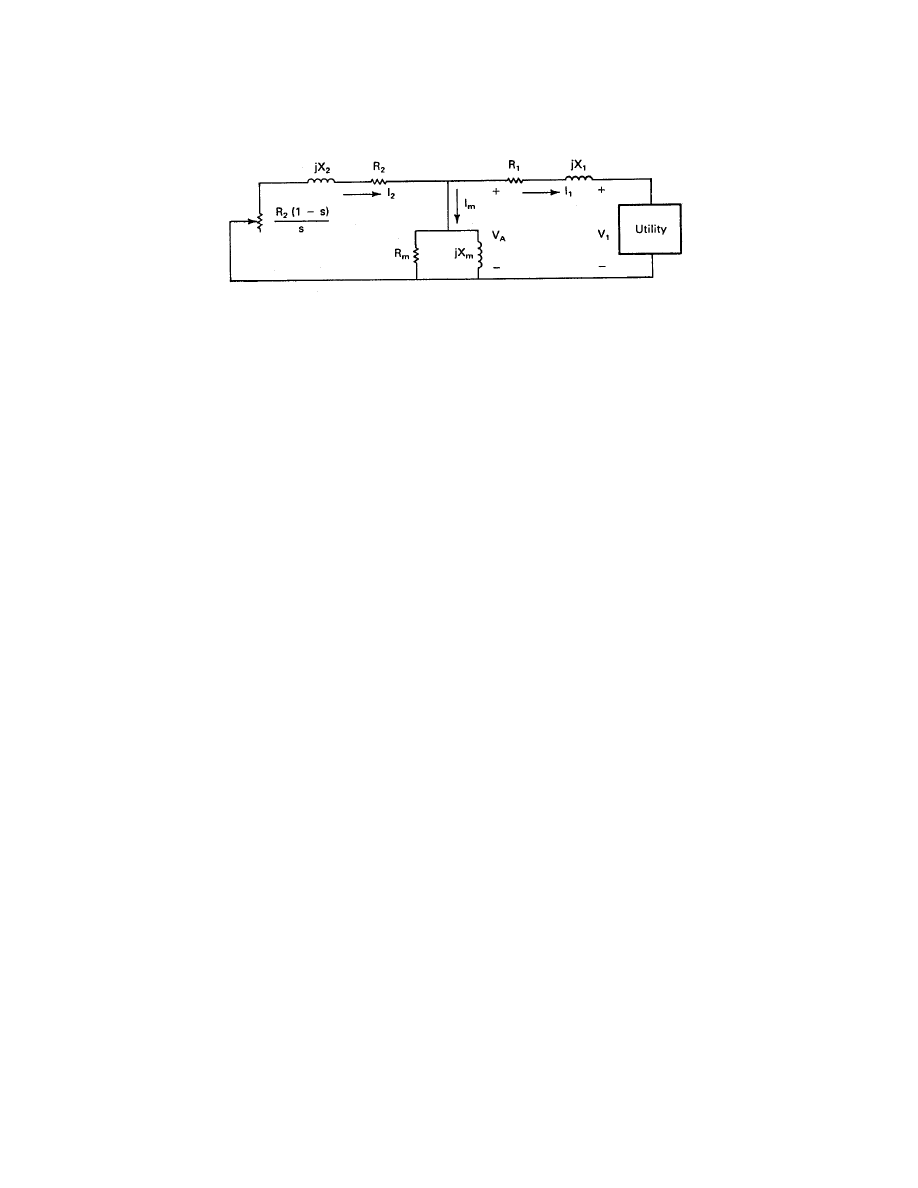
Chapter 5—Electrical Network
5–32
Figure 19: Equivalent circuit of one phase of an induction generator.
generator receives no reactive power and is not able to generate real power. This makes it
somewhat less versatile than the synchronous generator which is able to supply both real
and reactive power to the grid. The induction generator requirement for reactive power can
also be met by capacitors connected across the generator terminals. If the proper values of
capacitance are selected, the generator will operate in a self-excited mode and can operate
independently of the utility grid. This possibility is examined in Chapter 6.
The rated electrical output power of the induction generator will be very close to the rated
electrical input power of the same machine operated as a motor. If we maintain the same
rated current I
1
at rated voltage V
1
for both generator and motor operation, the machine will
have the same stator copper losses. The rotor current is proportional to I
2
and will be larger
for generator operation than for motor operation, as can be seen by comparing Fig. 17 and
Fig. 19. This will increase the rotor losses somewhat. The machine is running at 3-5 percent
above synchronous speed as a generator, so windage and friction losses are somewhat higher
than for motor operation. The saturation of the iron in the machine will be somewhat higher
as a generator so hysteresis and eddy current losses will also be somewhat higher. These
greater losses are counterbalanced by two effects. One is that the same wind which is driving
the turbine is also cooling the generator. A wind turbine application presents a much better
cooling environment to an induction machine than most applications, and this needs to be
included in the system design. The second effect is that the wind is not constant. Short
periods of overload would normally be followed by operation at less than rated power, which
would allow the machine to cool. These cooling effects should allow the generator rating to
be equal to the motor rating for a given induction machine.
It may well be that generator temperature will be used as a control signal for overload
protection rather than generator current or power. The generator is not harmed by delivering
twice its rated power for some period of time as long as its rated temperature is not exceeded.
Using temperature as a control variable will therefore fully utilize the capability of the machine
and allow a somewhat greater energy production than would be possible when using power
or current as the control variable.
The analysis of the induction generator proceeds much the same as the analysis of the
induction motor. The expressions for impedance in Eqs. 52 –54 keep the same form. The
negative slip causes the real parts of Z
2
and Z
in
to be negative, but this is easily carried along
Wind Energy Systems by Dr. Gary L. Johnson
November 21, 2001
Chapter 5—Electrical Network
5–33
in the computations. The change in assumed direction for I
1
and I
2
forces us to write their
equations as
I
1
=
−
V
1
Z
in
(63)
I
2
=
−
V
A
Z
2
(64)
The voltage V
A
is given by
V
A
= V
1
+ I
1
(R
1
+ jX
1
)
(65)
The real power P
m
supplied by the turbine is the same as Eq. 51. The negative sign
resulting from negative slip just means that power is flowing in the opposite direction. P
m
is
now the input power so the generator efficiency η
g
would be given by
η
g
=
|P
m
| − P
loss
|P
m
|
(66)
The total real power delivered to the utility by the generator is
P
e
= 3
|V
1
||I
1
| cos θ
W
(67)
where V
1
is the line to neutral voltage and θ is the angle between voltage and current as
defined by Eq. 16.
The total reactive power Q required by the generator is given by
Q = 3|I
2
|
2
X
2
+
3
|V
A
|
2
X
m
+ 3
|I
1
|
2
X
1
var
(68)
It is also given by the expression
Q = 3|I
1
||V
1
| sin θ
var
(69)
Example
A three-phase, Y-connected, 220-V (line to line), 10-hp, 60-Hz, six-pole induction machine has the
following constants in ohms per phase:
R
1
= 0.30 Ω/phase
R
2
= 0.14 Ω/phase
R
m
= 120 Ω/phase
X
1
= X
2
= 0.35 Ω/phase
X
m
= 13.2 Ω/phase
Wind Energy Systems by Dr. Gary L. Johnson
November 21, 2001
Chapter 5—Electrical Network
5–34
For a slip s = 0.025 (operation as a motor), compute I
1
, V
A
, I
m
, I
2
, speed in r/min, total output
torque and power, power factor, total three-phase losses, and efficiency.
The applied voltage to neutral is
V
1
=
220
√
3
= 127/0
o
V/phase
Z
2
=
R
2
s
+ jX
2
=
0.14
0.025
+ j0.35 = 5.60 + j0.35 = 5.61/3.58
o
Ω
Z
m
=
jR
m
X
m
R
m
+ jX
m
=
j(120)(13.2)
120 + j13.2
=
1584/90
o
120.72/6.28
o
= 13.12/83.72
o
Ω
Z
in
= R
1
+ jX
1
+
Z
m
Z
2
Z
m
+ Z
2
= 0.30 + j0.35 +
(13.12/83.72
o
)(5.61/3.58
o
)
13.12/83.72
o
+ 5.61/3.58
o
= 5.29/27.08
o
Ω
I
1
=
V
1
Z
in
=
127/0
o
5.29/27.08
o
= 24.01/ − 27.08
o
A
V
A
=
V
1
− I
1
(R
1
+ jX
1
) = 127
− 24.01/ − 27.08
o
(0.30 + j0.35)
=
116.76 − j4.20 = 116.84/ − 2.06
o
V
I
m
=
V
A
Z
m
=
116.84/ − 2.06
o
13.12/83.72
o
= 8.91/ − 85.78
o
A
I
2
=
V
A
Z
2
=
116.84/ − 2.06
o
5.61/3.58
o
= 20.83/ − 5.64
o
A
From Eq. 48 we have
n
s
=
7200
6
= 1200 r/min
From Eq. 47 the speed is
n = (1 − s)n
s
= (1
− 0.025)1200 = 1170 r/min
Wind Energy Systems by Dr. Gary L. Johnson
November 21, 2001
Chapter 5—Electrical Network
5–35
The total torque is given by Eq. 62.
T
m
=
90
|I
2
|
2
R
2
πn
s
s
=
90(20.83)
2
(0.14)
π(1200)(0.025)
= 58.01 N · m/rad
The total mechanical power is then
P
m
= ω
m
T
m
=
2πnT
m
60
=
2π(1170)(58.01)
60
= 7107 W
At 746 W/hp, the motor is delivering 9.53 hp to the load. From Eq. 17, the power factor is the cosine
of the angle between the input voltage and current, or in this case,
pf = cos 27.08
o
= 0.890 lag
From Eq. 49 the total three-phase losses are
P
loss
=
3(116.84)
2
120
+ 3(24.01)
2
(0.30) + 3(20.83)
2
(0.14) = 1042 W
The efficiency is given by Eq. 59.
η
m
=
P
m
P
m
+ P
loss
=
7107
7107 + 1042
= 0.872
The efficiency is 87.2 percent, a typical value for induction motors of this size.
Example
For the machine of the previous example, compute the input current, total starting torque, and
total three-phase losses while the machine is being started (while the slip is still essentially unity).
Assume the source is able to maintain rated voltage during the start.
With the slip s = 1, the impedance Z
2
becomes
Z
2
=
0.14
1
+ j0.35 = 0.377/68.20
o
Ω
The shunt impedance Z
m
remains the same as before. The input impedance is then
Z
in
= 0.30 + j0.35 +
13.12/83.72
o
(0.377/68.20
o
)
13.12/83.72
o
+ 0.377/68.20
o
= 0.816/57.92
o
Ω
I
1
=
127/0
o
0.816/57.92
o
= 155.58/ − 57.92
o
A
V
A
= 127
− 155.58/ − 57.92
o
(0.30 + j0.35) = 57.07/ − 10.73
o
V
Wind Energy Systems by Dr. Gary L. Johnson
November 21, 2001

Chapter 5—Electrical Network
5–36
I
2
=
57.07/ − 10.73
o
0.377/68.2
o
= 151.38/ − 78.93
o
A
The total torque is
T
m
=
90
|I
2
|
2
R
2
πn
s
s
=
90(151.38)
2
(0.14)
π(1200)(1)
= 76.59 N · m/rad
This torque is 1.25 times the rated running torque for this particular machine. A majority of induction
motors will have a starting torque which is about double the rated running torque.
The total three-phase losses will be
P
loss
=
3(57.07)
2
120
+ 3(155.58)
2
(0.30) + 3(151.38)
2
(0.14) = 31, 500 W
This number is about 30 times the loss term for the machine operating at full load. Also, when the
machine is not rotating, it is not able to circulate any air for cooling, which makes the temperature rise
even more severe. The stator windings will have the most rapid temperature rise for starting conditions
because of higher resistance, lower specific heat capacity, and poorer heat conductivity than the rotor
windings. This temperature rise may be on the order of 10
o
C/s as long as the rotor is not moving.
Obviously, the motor will be damaged if this locked rotor situation continues more than a few seconds.
An unloaded motor will typically start in 0.05 s and one with a typical load will usually start in
less than 1 s, so this heating is not normally a problem. If a very high inertia load is to be started,
such as a large Darrieus, a clutch may be necessary between the motor and the turbine. Very large
motors may need special starting techniques even with a clutch. These will be discussed in the next
section.
Example
The induction machine of the previous example is operated as a generator at a slip of -0.025.
Terminal voltage is 220 V line to line. Find I
1
, I
2
, input power P
m
, output power P
e
, reactive power
Q, and efficiency η
g
. If the rated I
1
is 25 A when operated as a motor, comment on the amount of
overload, if any.
From the previous example we have V
1
= 127/0
o
. The impedance Z
2
is given by
Z
2
=
0.14
−0.025
+ j0.35 = 5.61/176.42
o
Ω
Z
in
= 0.30 + j0.35 +
13.12/83.72
o
(5.61/176.42
o
)
13.12/83.72
o
+ 5.61/176.42
o
= 5.16/147.90
o
Ω
I
1
=
−
127/0
o
5.16/147.90
o
=
−24.60/ − 147.90
o
= 24.60/32.10
o
A
Wind Energy Systems by Dr. Gary L. Johnson
November 21, 2001

Chapter 5—Electrical Network
5–37
V
A
= 127 + 24.60/32.10
o
(0.30 + j0.35) = 129.16/4.98
o
V
I
2
=
−129.16/4.98
o
5.61/176.42
o
=
129.16/184.98
o
5.61/176.42
o
= 23.02/8.56
o
A
The total input mechanical power P
m
is
P
m
=
3
|I
2
|
2
R
2
(1
− s)
s
=
3(23.02)
2
(0.14)(1 + 0.025)
−0.025
=
−9125 W
The machine was delivering 9.53 hp to the mechanical load as a motor, but is now requiring 12.23 hp
as mechanical shaft power input as a generator. The total output power is
P
e
= 3
|V
1
||I
1
| cos θ = 3(127)(24.60) cos(−32.10
o
) = 7940 W
The total reactive power Q is
Q = 3|V
1
||I
1
| sin θ = 3(127)(24.60) sin(−32.10
o
) =
−4980 var
The negative sign means that the induction generator is supplying negative reactive power to the
utility, which is the same as saying it is receiving positive reactive power from the utility.
We can compute the efficiency by computing the losses from Eq. 49 and using Eq. 61, or we can
merely take the ratio of output to input power.
η
g
=
|P
e
|
|P
m
|
=
7940
9125
= 0.870
The output current of 24.60 A is slightly under the rated current of 25 A. If the machine is well
ventilated, it should operate at this current level for an indefinite period of time.
6 MOTOR STARTING
Small induction motors with low to medium inertia loads are normally started by direct con-
nection to a source of rated voltage. Above a rated power of a few kW, the high starting
currents usually cause a reduction in line voltage. This reduction may prevent the motor from
developing adequate torque to start its load. Electronic equipment and lighting circuits con-
nected to the same source may also be affected by these voltage fluctuations. It is customary,
therefore, to start the large induction motors on lowered voltages to limit the starting currents
and line voltage fluctuations.
This practice is not essential if the supply has sufficient capacity to supply the starting
current without objectionable voltage reduction. Motors with ratings up to several thousand
Wind Energy Systems by Dr. Gary L. Johnson
November 21, 2001

Chapter 5—Electrical Network
5–38
kW are routinely started across line voltage in generating stations, where a starting current of
5 to 10 times the rated current can easily be supplied. The motor itself will not be damaged
by these high currents unless they are sustained long enough to overheat the motor.
There are three basic ways to accomplish reduced-voltage starting. These are illustrated
in Fig. 20.
1. Line resistance or reactance starting uses series resistances or reactances in each line to
provide a voltage drop and reduce the voltage at the motor terminals. After a suitable
time delay these components are removed in one or more steps. The notation L
1
, L
2
,
and L
3
refers to the three phases of the incoming power line.
2. Autotransformer starting uses tapped autotransformers to reduce the motor voltage.
These taps normally provide between 50 and 80 percent of rated voltage.
3. Wye-delta starting is used when the motor is designed for delta operation but has both
ends of each phase winding available external to the motor. The phase windings are
reconnected by contactors into a wye circuit for starting. Once the motor is running, it
is changed back to its normal delta configuration. This technique reduces the voltage
seen by each phase by the factor
√
3.
Complete circuits would include push button start and stop, fuses, and undervoltage pro-
tection as well as other features to meet electrical codes. In each case a triple-pole switch is
moved to the start position until the motor has accelerated the load to almost full speed, and
then rapidly thrown to the run position, so that the motor is connected directly across the
line.
The autotransformer has the same characteristic as a two winding transformer in that the
input and output apparent power in kVA have to be the same, except for any transformer
losses. Fig. 21 shows an autotransformer supplying power to an induction motor. V
L
and I
L
are the voltage and current supplied by the line and V
1
and I
1
are the voltage and current
delivered to the motor. For an ideal transformer
V
L
I
L
= V
1
I
1
(70)
Transformer operation requires that V
1
be less than V
L
, which means I
L
will be less
than I
1
. Because of the nature of the load, when V
1
is reduced below its rated value, I
1
will also be reduced. The starting current supplied by the line is therefore reduced by both
the autotransformer action and by the reduced motor voltage, which makes autotransformer
starting rather popular on limited capacity lines.
Example
An autotransformer starting system is used to reduce the voltage to the motor of the examples in
the previous section to 0.6 of its rated value. Find the motor starting current I
1
, the line current input
I
L
to the autotransformer, the total motor losses at start, and the total starting torque.
Wind Energy Systems by Dr. Gary L. Johnson
November 21, 2001
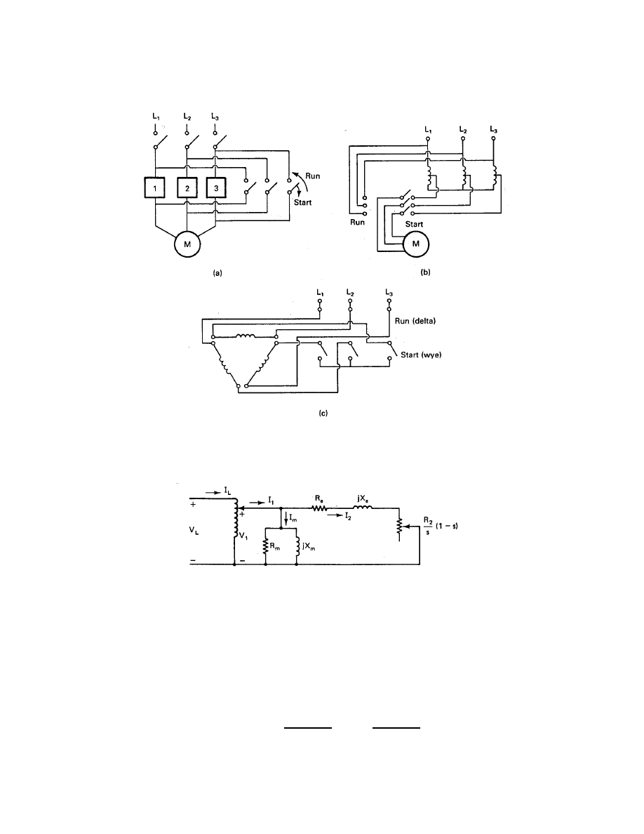
Chapter 5—Electrical Network
5–39
Figure 20: Starting methods for induction motors: (a) line resistance or reactance starting;
(b) autotransformer starting; (c) wye-delta starting.
Figure 21: Circuit for autotransformer start of induction motor.
The applied voltage to the motor is
V
1
= 0.6(127) = 76.2 V/phase
The input starting current is also 0.6 of its value from the previous example on motor starting current.
I
1
= 0.6(155.58/ − 57.92
o
) = 93.35/ − 57.92
o
A
Wind Energy Systems by Dr. Gary L. Johnson
November 21, 2001

Chapter 5—Electrical Network
5–40
Similarly,
I
2
= 0.6(151.38/ − 78.93
o
) = 90.83/ − 78.93
o
A
From Eq. 70 the input current to the autotransformer is
I
L
=
V
1
I
1
V
L
=
(76.2)(93.35/ − 57.92
o
)
127
= 56.01/ − 57.92
o
A
This is only a little more than twice the rated running current of the motor, hence should not cause
substantial voltage fluctuations.
The total motor losses will be
P
loss
=
3[(0.6)(57.07)]
2
120
+ 3(93.35)
2
(0.30) + 3(90.83)
2
(0.14) = 11, 340 W
which is (0.6)
2
= 0.36 of the losses during the full voltage start. This is still an order of magnitude
greater than the operating losses at full load and would result in damage to the motor if it does not
start within 10 to 20 seconds.
The total starting torque is
T
m
=
90(90.83)
2
(0.14)
π(1200)(1)
= 27.57 N · m/rad
which is about 46 percent of rated torque. If this torque is not adequate to start the motor load, then
the autotransformer taps can be changed to provide a larger starting voltage of perhaps 0.7 or 0.8
times rated voltage, at the expense of larger line currents.
7 CAPACITY CREDIT
Wind generators connected to the utility grid obviously function in the role of fuel savers.
Their value as a fuel saver may be quite adequate to justify their deployment, especially in
utilities that depend heavily on oil fired generating plants. The value to a utility may be
increased, however, if the utility could defer building some conventional generating plants
because of the wind turbines presence on the grid. Wind generators would have to have some
effective load carrying capability in order to receive such a capacity credit.
Some may feel that since the wind may not blow at the time of the yearly peak load
that the utility is forced to build generation equipment to meet the load without considering
the wind, in which case the wind cannot receive a capacity credit. This is not a consistent
argument because any generating plant may be unavailable at the time of the peak load, due
to equipment failure. The lack of wind is no different in its effect than an equipment failure,
and can be treated in a standard mathematical fashion to determine the effective capacity of
the wind generator.
Wind Energy Systems by Dr. Gary L. Johnson
November 21, 2001

Chapter 5—Electrical Network
5–41
One way of approaching the question of capacity credit is to consider the wind turbine
as an alternative to other types of generation which might be installed by the utility. There
is general agreement that the correct criterion for the economic selection of a generating
unit is that its cost, when combined with the costs of other generating units making up a
total electric utility generating system, should result in a minimum cost of electricity. The
established method of checking this criterion is to simulate the total utility system cost over a
period of time which represents a major fraction of the life of the unit being considered. The
first step in this process is to define alternate expansions of the system capacity which will
have equal reliability in serving the forecasted load. Annual production costs (fuel, operation
and maintenance) are determined by detailed simulation methods. To these costs are added
annual fixed charges on investment, giving total annual revenue requirements. The expansion
having lowest present worth of revenue requirements is the economic choice. These economic
terms will be discussed further in Chapter 8. The procedures of total utility system cost
analysis have been understood and applied for many years, but tend to be complex, costly
to use, and time consuming. There is thus a natural tendency to use shortcuts, at least in
preliminary analyses.
One shortcut to the detailed simulation method which normally extends over 20 to 30
years is a detailed simulation for a single year. The effect of a changing mix of generation
on future production costs can be approximately evaluated by selecting two years for detailed
simulation, one at the beginning of the study period and the other at the end. This shortcut
will normally give adequate results for preliminary analyses.
This simulation requires that we have a complete year of hourly wind data. This needs
to be as typical as possible, which is difficult to determine because of the inherent variability
of the wind. If the simulation results of one year suggest that the wind generator may be
economically feasible, then perhaps nine other years of wind data need to be passed through
the computer.
The range of system yearly costs will help establish the actual economic
feasibility of the wind generator. Such long time spans of good wind data collected at hub
height, or at least 50 m, are not readily available, but are badly needed for these analyses.
Production costs for the simulation year are determined by standard utility techniques.
Each generating plant is assigned a scheduled maintenance period. This is a period of typically
4 to 6 weeks each year for coal and nuclear plants, during which the plant is shut down, the
turbine is taken apart and cleaned, and other routine and preventive maintenance is performed.
These periods are normally scheduled during staggered periods in the spring and fall when
the demand for electricity is relatively low.
Operation of the remaining units is scheduled on a chronological, hourly basis. The most
economical plants are placed in service first and the least economical last. Nuclear plants have
low fuel costs so are operated at maximum power as much as possible. Such plants which are
operated a maximum amount are called base load plants. Base load coal units are scheduled
next, followed by intermediate load and load following coal and oil fired units, which are
followed by oil and gas fired peaking turbines. Generation with zero fuel cost, such as hydro
and wind, is used as much as possible to reduce operating costs.
Wind Energy Systems by Dr. Gary L. Johnson
November 21, 2001

Chapter 5—Electrical Network
5–42
The utility bases its plans for expansion on the need to maintain a reliable system. Utilities
try to maintain a total installed capacity at least 15 percent greater than the expected yearly
peak load. This allows them to continue to meet the required load even if a large generating
plant has a forced outage. When the load is not at its peak, several generating plants may
have forced outages without affecting the ability of the utility to meet its load with its own
generation.
There is a certain probability of a forced outage occurring during a daily operation cycle.
This probability varies with the type, age, and general condition of the generating plant. A
typical forced outage rate for a hydro plant may be 1.5 percent, while that of a coal fired plant
may be 5 percent. A 5 percent forced outage rate means that, on the average, a given plant
will be out of service at least a part of the day for one day out of twenty. Forced outages
typically take the plant out of service for at least 24 hours before repairs are made and the
plant is put back on the line, so the daily peak load would normally occur while the forced
outage is present. This means that the daily peak is used in determining reliability of a system
rather than hourly loads.
The probability of two generating plants being on forced outage at the same time is just
the product of the probabilities that either one will be out. If each has a forced outage rate of
0.05, the probability of both being forced out at the same time is (0.05)
2
= 0.0025 or about
0.91 days per year. The probability of additional generation being out at this same time is
still smaller, of course.
Suppose for the sake of illustration that we have a utility system with ten 700 MW gen-
erators, each with a forced outage rate of 0.05. Suppose that the load for several days is as
shown in Fig. 22. The peak load for the first day is between 4900 and 5600 MW, so three
generating plants have to be out of service before the utility is unable to meet its load. Two
plants being out will cause a loss of load on the third day while four plants would have to
be out on the fifth day to cause a loss of load. If the load ever exceeds 7000 MW then the
probability of generation being inadequate that day is 1.0
Each day has a certain probability R
d
(daily risk) that generation will be inadequate to
meet the load. If we add these daily risks for an entire year, we get an annual risk R
a
,
expressed in days per year that generation will be inadequate[3].
R
a
=
365
i=1
R
d
(i)
(71)
Example
The daily peak load on the model utility system of Fig. 22 is between 3500 and 4200 MW for 150
days of the year, between 4200 and 4900 MW for 120 days, between 4900 and 5600 MW for 60 days,
and between 5600 and 6300 for 35 days. What is the annual risk R
a
?
Wind Energy Systems by Dr. Gary L. Johnson
November 21, 2001
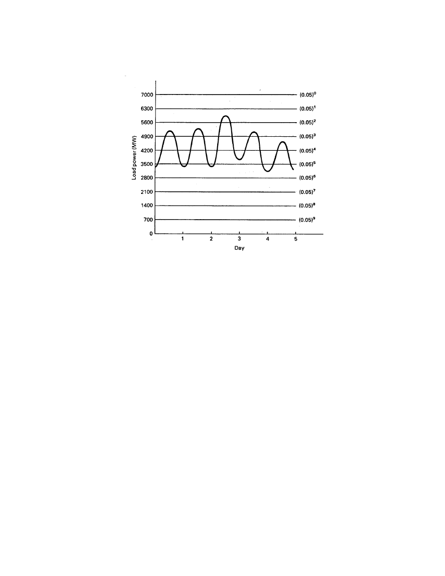
Chapter 5—Electrical Network
5–43
Figure 22: Load variation in model utility system.
R
a
=
365
i
=1
R
d
(i) = 150(0.05)
5
+ 120(0.05)
4
+ 60(0.05)
3
+ 35(0.05)
2
=
4.6875 × 10
−5
+ 7.5 × 10
−4
+ 7.5 × 10
−3
+ 87.5 × 10
−3
=
95.8 × 10
−3
= 0.0958 day per year
This result shows that generation is inadequate to meet load about 0.1 days per year or about one
day in ten years. This level of reliability is a typical goal in the utility industry.
We see that a relatively small number of days with the highest peak load contributes the largest part
of the annual risk. If these peaks could somehow be reduced through conservation or load management,
system reliability would be improved.
It should be emphasized that even when load exceeds the rating of generators on a system,
the utility may still meet its obligations by purchasing power from neighboring utilities or by
dropping some less critical loads. Only when the generation of many utilities is inadequate
will load actually be lost.
The effective capability or effective capacity of a proposed generating plant is determined
in the following manner. The annual risk is determined for the original system for the year
under investigation. This requires a loss-of-load probability calculation based on (1) the rating
Wind Energy Systems by Dr. Gary L. Johnson
November 21, 2001
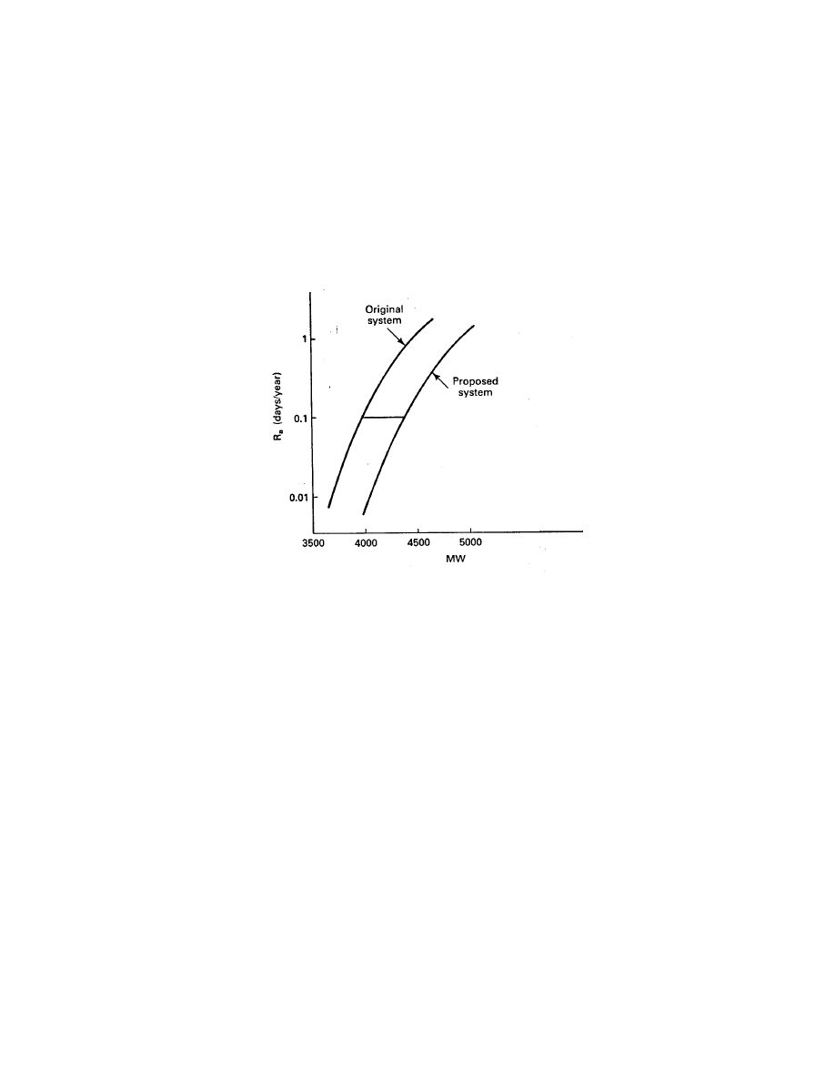
Chapter 5—Electrical Network
5–44
of each generating plant and its forced outage rate, (2) the daily hourly-integrated peak loads
(the greatest energy sales in any one hour of the day), (3) maintenance requirements for
each unit, and (4) other special features such as seasonal deratings or energy interchange
contracts.
The single point resulting from this calculation is spread out into a curve by
varying the assumed annual peak load for that year by
±20 percent and each daily peak by
the same fraction. As the assumed peak load increases for the same generation, the annual
risk increases. A curve such as the original system curve of Fig. 23 is the result.
Figure 23: Annual risk before and after adding a new unit.
The proposed new generating plant is then added to the system while keeping all other
data fixed. We again vary the annual peak load with the daily peaks considered as a fixed
percentage of the annual peak. Adding this unit reduces the risk at a given load, so we
consider a somewhat larger range of loads, perhaps a zero to 40 percent increase over the
previous midpoint load. The result can be plotted into the second curve of Fig. 23. The
distance in megawatts between these curves at the desired risk level is the amount of load
growth the system can accept and still retain the same reliability. This distance is the effective
capability or effective capacity of the new unit. The effective capacity will typically be between
60 and 85 percent of rated capacity for new fossil or nuclear power plants. If it is at 75 percent,
this means that a 1000-MW generating plant will be able to support 750 MW of increased
load. The remaining 250 MW will be considered reserve capacity.
The effective capacity is not identical to the capacity factor or plant factor, which was
defined in Chapter 4 as the ratio of average power production to the rated power. Capacity
factor is calculated independently of the timing of the load cycle, while effective capacity
includes the effect of the utility hourly demand profile. Effective capacity may be either
larger or smaller than the capacity factor.
An oil fired gas turbine may have an actual
Wind Energy Systems by Dr. Gary L. Johnson
November 21, 2001
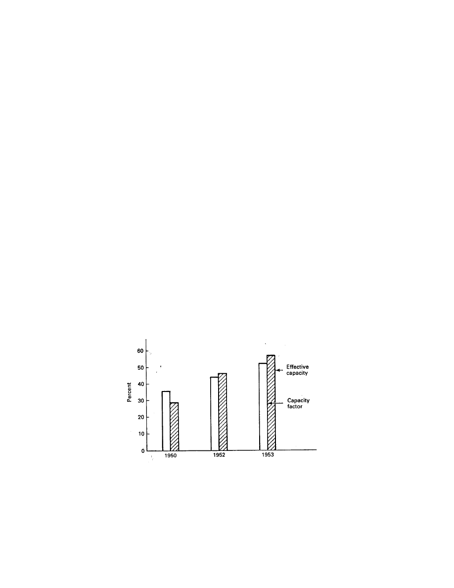
Chapter 5—Electrical Network
5–45
capacity factor of less than 10 percent because of the limited hours of operation, but have
an effective capacity of nearly 90 percent because of its high availability when the peak loads
occur. Wind electric plants will almost always be operated when the wind is available because
of the zero fuel cost. If the wind blows at the rated wind speed half the time and is calm the
other half of the time, then the capacity factor would be 0.5 except for the reduction due to
forced and planned outages. If the winds occurred at the times of the utility peaks, then the
effective capacity would be close to unity. However, if the wind is calm when the utility peaks
are occurring, the effective capacity will be near zero. The timing of the wind plant output
relative to the utility hourly demand profile is critical.
General Electric has performed a large study to determine the effective capacity of wind
turbines on actual utility systems[5]. They selected a site in Kansas, another in New York,
and two in Oregon. Detailed data for Kansas Gas and Electric, Niagara Mohawk, and the
Northwest Power Pool were analyzed using state-of-the-art computer programs. Actual load
data and actual wind data were used. Results are therefore rather specific and somewhat
difficult to extrapolate to other sets of circumstances.
However, they represent the best
possible estimate of capacity factor and effective capacity that could be obtained at the time
of the study, and are therefore quite interesting.
Figure 24 shows the effective capacity and capacity factor for wind turbines on the assumed
1990 Kansas Gas and Electric System. Dodge City wind data for the years 1950, 1952, and
1953 were used in the study. These wind data were recorded at 17.7 m and extrapolated
to hub height of a model 1500 kW horizontal axis, constant speed wind turbine by the one-
seventh power law equation. A total wind generation capacity of 163 MW or 5 percent of
total capacity was assumed. This is often referred to as a penetration of 5 percent. A forced
outage rate of 5 percent was also assumed. There is no energy storage on the system.
Figure 24: Impact of weather year on capacity factor and effective capacity.
It may be seen that effective capacity varies from less than 30 percent in 1950 to almost
Wind Energy Systems by Dr. Gary L. Johnson
November 21, 2001

Chapter 5—Electrical Network
5–46
60 percent in 1953. It can also be seen that the effective capacity is slightly larger than the
capacity factor for two years and smaller for the third year. The particular year of wind data
thus makes a substantial impact on the results. The representiveness of the year or years
selected must therefore be considered before any firm conclusions are drawn.
The theoretical output of a MOD-0 located at Dodge City was determined for the years
1948 through 1973 in a attempt to determine the year-to-year variability[6]. The monthly
energy production of each m
2
of turbine swept area is shown in Table 5.2 for each of the years
in question, as well as the mean and standard deviation for all 26 years. The yearly standard
deviation of 39.97 kWh/m
2
was computed from the yearly means rather than the sum of the
monthly standard deviations. It may be seen that 1950 was two standard deviations below the
mean. The only year worse than 1950 in this 26 year period was 1961 with 349.6 kWh/m
2
. The
year 1952 is close to the 26 year mean, but the summer months are somewhat above the mean,
which tends to improve the effective capacity in this summer peaking utility. The year 1953
is about one standard deviation above the mean. The only year better than 1953 is 1964 with
518.8 kWh/m
2
. We see that the three years selected cover the range of possible performance
rather well. As more and better wind data become available, statistical limits can be defined
with greater precision and confidence. In the meantime, for Dodge City winds, Kansas Gas
and Electric loads, and a model 1500 kW wind turbine with 5 percent penetration, a reasonable
estimate for capacity factor is a value between 35 and 50 percent. The corresponding estimate
for effective capacity is between 30 and 55 percent of rated capacity. Other wind regimes and
other load patterns may lead to substantially different results, of course.
The effective capacity of the wind plant tends to saturate as more and more of the utility
generation system consists of this intermittent random power source. The study assumes
that the wind is the same over the entire utility area (no wind diversity) so all the wind
generators tend to act as a single generator. The utility needs to have enough generation
to cover the loss of any one generator, so penetration levels above 15 or 20 percent of total
system capacity would not have much effective capacity. Large amounts of storage would be
required to maintain system reliability at higher penetration levels.
Figure 25 shows the variation in effective capacity with penetration for the four cases
mentioned earlier. There is a wide variation, as might be expected, with Kansas Gas and
Electric being the best and the Columbia River Gorge site of the Northwest Power Pool being
the worst. The capacity factors for these two cases were almost identical, or about 45 percent
for the wind years chosen. The reason for the low effective capacity at the Gorge site is that
the bulk of the annual risk R
a
is obtained from just a few days in the Northwest Power Pool,
and the wind did not blow on those days in the particular wind year selected.
In a system like the Northwest Power Pool, wind diversity would be expected to improve
the effective capacity, perhaps a significant amount. One test case showed that the combined
output of wind turbines at both the Gorge and coast sites had a higher effective capacity than
either site by itself. More computer studies are needed to determine the actual advantages of
diversity.
Wind Energy Systems by Dr. Gary L. Johnson
November 21, 2001
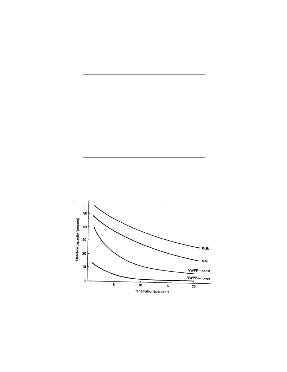
Chapter 5—Electrical Network
5–47
Table 5.2 Theoretical Energy Production of MOD-0
Located at Dodge City (kWh/m
2
)
Standard
1950
1952
1953
Mean
Deviation
Jan.
31.6
34.1
40.2
36.3
3.85
Feb.
29.5
35.0
41.8
37.5
3.60
Mar.
38.5
41.0
42.8
41.9
3.79
Apr.
36.0
39.4
43.1
42.3
4.41
May
37.4
33.9
44.3
40.3
4.50
Jun.
38.9
43.5
50.5
39.7
6.72
Jul.
26.8
41.5
38.2
35.3
6.40
Aug.
22.9
36.4
37.3
34.3
6.55
Sep.
24.3
37.1
37.2
37.2
4.58
Oct.
31.3
31.1
41.0
36.7
4.57
Nov.
28.2
36.4
37.9
35.1
5.39
Dec.
22.2
30.5
39.7
37.8
6.27
367.7
440.1
493.8
454.4
39.97
It would appear from the limited data that effective capacities of wind turbines may vary
from 10 to 60 percent for initial penetrations and from 5 to 45 percent at 5 percent penetration.
Hopefully, wind diversity will raise the lower limit to at least 15 or 20 percent. We conclude,
therefore, that wind turbines do have an effective capacity and that any complete cost analysis
should include a capacity credit for the wind machines as well as a fuel savings credit.
Figure 25: Wind power plant effective capacity versus penetration.
The actual capacity displaced, D
c
, depends on the effective capacities of both the wind
Wind Energy Systems by Dr. Gary L. Johnson
November 21, 2001

Chapter 5—Electrical Network
5–48
plant and the displaced conventional plant.
D
c
= P
e
R
E
w
E
c
(72)
In this equation D
c
is the displaced conventional capacity in kW or MW, P
e
R
is the rated
power of the wind plant, E
w
is the effective capacity of the wind plant, and E
c
is the effective
capacity of the conventional plant.
Example
A utility planning study shows that it needs to add 700 MW of coal fired generation to its system
to maintain acceptable reliability. The effective capacity of this generation is 0.75. What nameplate
rating of wind turbines with an effective capacity of 0.35 is required to displace the 700 MW of coal
generation?
From Eq. 72,
P
e
R
= D
c
E
c
E
w
= 700
0.75
0.35
= 1500 MW
For this particular situation, 1500 MW of wind generation is required to displace 700 MW of coal
generation from a reliability standpoint. If, for example, the capacity factor of the coal generation
was 0.7 and 0.4 for the wind generation, the wind turbines would produce more energy per year than
the displaced coal plant. This means that less fuel would be burned at some existing plant, so the
wind turbine may have both capacity credit and fuel saving credit. The utility system must meet both
reliability and energy production requirements, so adding wind turbines to maintain reliability may
force the capacity factors of other plants on the utility system to change. An example of the economic
treatment of this situation is given in Chapter 8.
8 FEATURES OF THE ELECTRICAL NETWORK
The electrical network in which the wind electric generators must operate is a rather sophis-
ticated system. We need to examine its organization so that we can better understand the
interaction of the wind generator with the electric utility.
Figure 26 shows a one line diagram of a portion of an electric utility system. Power is
actually transferred over three-phase conductors, but one line is used to represent the three
conductors to make the drawing easier to follow. We start the explanation of this figure with
the generating plant. This could be a large coal or nuclear plant, or perhaps a smaller gas
or oil fired generator. The generation voltage is limited to about 25,000 volts because of
generator insulation limitations. This is too low for long distance transmission lines, so it is
increased through a step-up transformer to one of the transmission voltages for the particular
utility. Some utilities use 115 kV, 230 kV, and 500 kV while others use 169 kV, 345 kV, and
765 kV. The higher voltage lines are used for transmitting greater power levels over longer
distances.
Wind Energy Systems by Dr. Gary L. Johnson
November 21, 2001
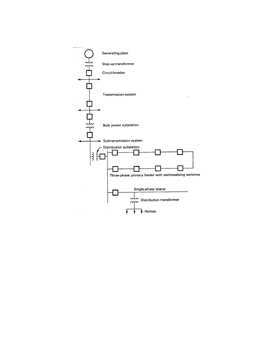
Chapter 5—Electrical Network
5–49
Figure 26: Typical electric utility system.
The next component shown in the one line diagram is a circuit breaker. This device is able
to interrupt large current flows and protect the various system components from short circuits.
If the short circuit were allowed to continue for a long period of time, even the transmission
line would overheat and be destroyed. The circuit breaker is activated by protective relays
which sense such parameters as voltage levels, current levels, frequency, and phase sequence
on the power line.
The power flows through the transmission line until it reaches a bulk power substation.
This is a collection of circuit breakers, switches, and transformers which connects the trans-
mission line to several lines in the subtransmission system if the utility has such a system.
The power then flows to a distribution substation where it is stepped down to distribution
Wind Energy Systems by Dr. Gary L. Johnson
November 21, 2001

Chapter 5—Electrical Network
5–50
voltages. The substation may feed a loop where every point in the loop can be reached from
two directions. This organization allows most of the loads along such a primary feeder to be
served even if a section of distribution line is not operable, due to storm damage, for example.
There will also be single-phase lateral or radial lines extending out from the distribution
substation.
These are connected to distribution transformers to supply 120/240 volts to
homes along the line. These lines generally operate at voltages between 2.4 and 34.5 kV.
These circuits may be overhead or underground, depending on the load density and the
physical conditions of the particular area to be served. Substation transformer ratings may
vary from as small as 1000 to 2500 kVA for small rural applications up to 50,000 or 60,000
kVA. Distribution transformer ratings are typically between 5 and 50 kVA.
The first responsibility of the design engineer is to protect all the utility equipment from
faults on the system. These faults may be caused by lightning, storm damage, or equipment
malfunction. When a fault occurs, line currents will be much larger than normal and a circuit
breaker will open the line. A simple distribution substation protection scheme is shown in
Fig. 27. The circuit breakers are adjusted so only the one nearest the fault will open. That
is, if a fault occurs on the load side of circuit breaker CB4, only CB4 will open. The others
will remain closed. Many of the circuit breakers in use are of the automatic reclosing variety,
where the circuit breaker will automatically reclose after a fraction of a second. If the fault
was caused by lightning, as it normally is, the electric arc between conductors will have time
to dissipate while the breaker is open, so service is restored with minimum inconvenience to
the customer. If the fault is still present when the breaker closes, it will open again, wait a
fraction of a second, and close a second time. If the fault is still present, the breaker will open
and remain open until the maintenance crew repairs the problem.
The larger transformers will be protected by differential current relays. This is a relay
which compares the input and output current of a transformer and opens a breaker when the
current ratio changes, indicating a fault within the transformer. There may be an underfre-
quency relay which will open a breaker if the utility frequency drops below some specified
value. A number of other protective devices are used if required by the particular situation.
Once the system is properly protected, the quality of electricity must be assured. Quality
refers to such factors as voltage magnitude, voltage regulation with load, frequency, harmonic
content, and balance among the three phases. The electric utility goes to great lengths to
deliver high quality electricity and uses a wide variety of methods to do so. We shall mention
only the methods of controlling voltage magnitude.
The voltage in the distribution system will vary with the voltage coming in from the
transmission lines and also with the customer load. It is adjusted by one or more of three
possible methods. These are transformer load tap changing, voltage regulators, and capacitor
banks. In the tap changing case, one of the transformer windings will have several taps
with voltage differences of perhaps two percent of rated voltage per tap. The feeders can be
connected to different taps to raise or lower the feeder voltage. This is done manually, perhaps
on a seasonal basis, but can also be done automatically. Automatic systems allow the taps to
Wind Energy Systems by Dr. Gary L. Johnson
November 21, 2001
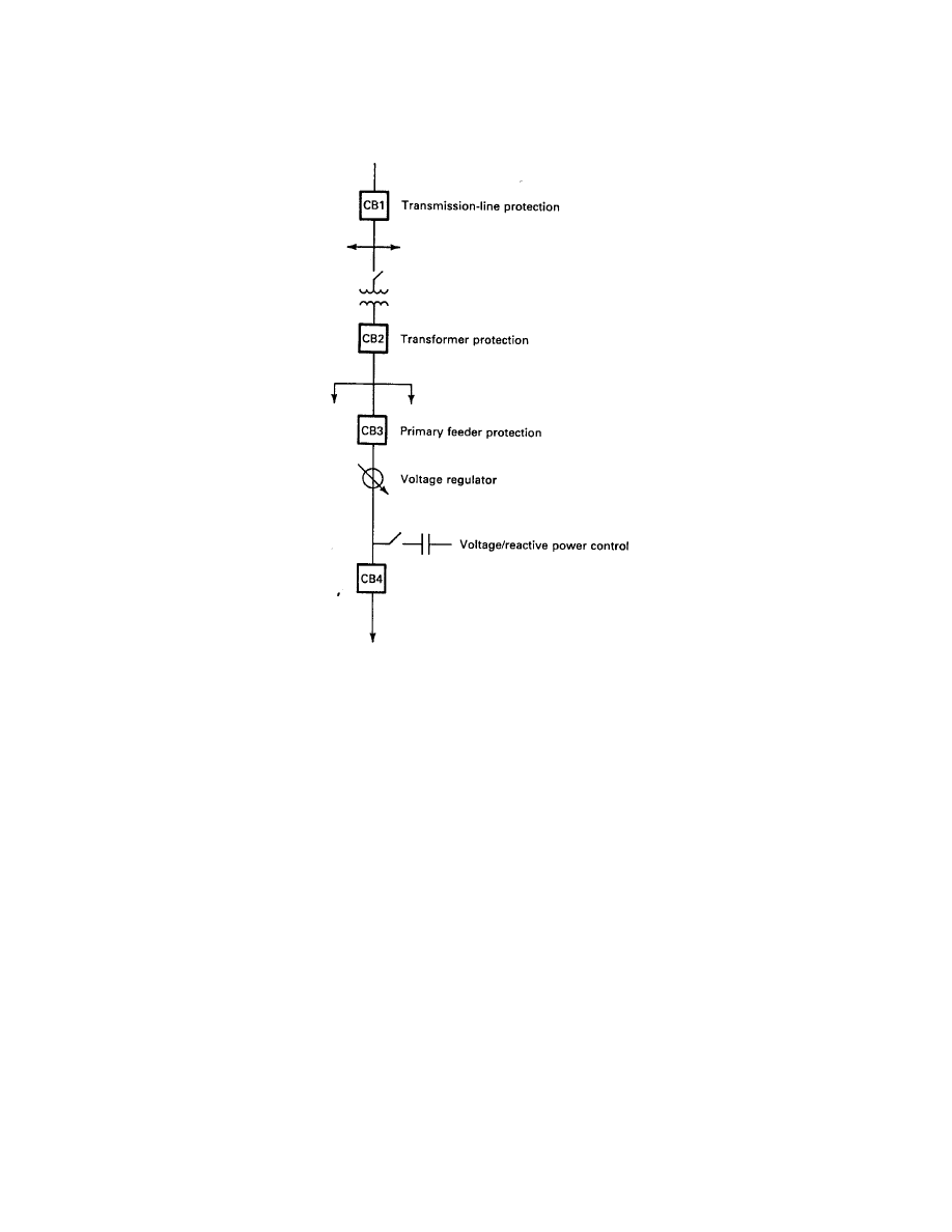
Chapter 5—Electrical Network
5–51
Figure 27: Distribution substation protection.
be changed several times a day to reflect changing load conditions.
The voltage regulator acts as an autotransformer with a motor driven wiper arm. This
can adjust voltage over a finer range than the tap changing transformer and responds more
rapidly to changes in voltage. It would be continually varying throughout the day as the loads
change.
Capacitor banks are used to correct the power factor seen by the substation toward unity.
This reduces the current flow in the lines and raises the voltage. They are commonly used
on long distribution lines or highly inductive loads. They may be located at the substation
but are often scattered along the feeder lines and at the customer locations. They may be
manually operated on a seasonal basis or may be automatically switched in or out by a voltage
sensitive relay.
All of these voltage control devices operate on the assumption that power flows from the
substation to the load and that voltage decreases with increasing distance from the substation.
A given primary feeder may have 102 percent of rated voltage at the substation and 98 percent
Wind Energy Systems by Dr. Gary L. Johnson
November 21, 2001

Chapter 5—Electrical Network
5–52
at the far end, for example. This assumption is not necessarily valid when wind generators are
added to the system. Power flow into the feeder is reduced and may even be reversed, in which
case the line voltage will probably increase as one gets closer to the wind generator. We may
have a voltage regulator that is holding the primary feeder voltage at 102 percent of rated, as
before, but now the voltage at the far end may be 106 percent of rated, an unacceptably high
value. It should be evident that wind generators can not be added to a distribution system
without careful attention being given to the maintenance of the proper voltage magnitude at
all points on the system.
We see in this simple example a need for greater or more sophisticated monitoring and
control as wind generators are added to a power system. Existing power systems already
have very extensive monitoring and control systems and these are becoming increasingly more
complex to meet the needs of activities like load management and remote metering. We shall
now briefly examine utility requirements for monitoring and control of their systems.
The structure of the power monitoring and control system in the United States is shown
in Fig. 28. It can be seen that there are many levels in this system. At the top is the National
Electric Reliability Council and the nine Regional Councils. These Regional Councils vary in
size from less than one state (Electric Reliability Council of Texas (ERCOT)) to the eleven
western states plus British Columbia (Western Systems Coordinating Council (WSCC)). Some
of the Regional Councils function as a single power pool while others are split into smaller
collections of utilities, covering one or two states. A power pool is a collection of neighboring
utilities that cooperate very closely, both in daily operation of an interconnected system and
in long range planning of new generation.
The reliability councils are primarily concerned with the long range planning and the
policy decisions necessary to assure an adequate and reliable supply of electricity. They are
usually not involved with the day to day operation of specific power plants.
Each power pool will have an operating center which receives information from its member
utilities. This operating center will also coordinate system operation with other power pools.
Each large power plant will have its own control center. There may also be distribu-
tion dispatch centers which control the operation of substations, distribution lines, and other
functions such as solar thermal plants, wind electric generators, storage systems, and load
management, and gather the necessary weather data. Some utilities will not have separate
distribution dispatch centers but will control these various activities from the utility dispatch
center.
It should be mentioned that each utility is a separate company and that their association
with one another in power pools is voluntary. The utilities will coordinate both the long
term planning of new power plants and the day to day operation of existing plants with
their neighbors in order to improve reliability and to reduce costs. Each utility tries to build
enough generation to meet the needs of its customers, but there are periods of time when it
is economically wise for one utility to buy electricity from another. If load is increasing by
100 MW per year and a 700-MW coal plant is the most economical size to build, a utility
Wind Energy Systems by Dr. Gary L. Johnson
November 21, 2001
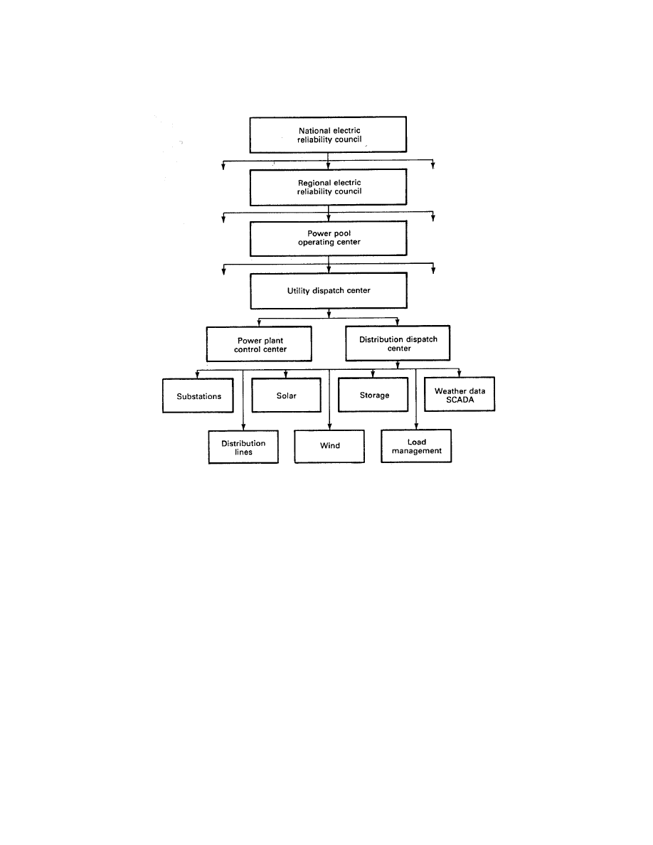
Chapter 5—Electrical Network
5–53
Figure 28: Monitoring and control hierarchy.
may want to buy electricity from another utility for two or three years before this coal plant
is finished and then sell the surplus electricity for three or four years until the utility is able
to use all of its capacity.
There are also times when short term sales are economically wise. One utility may have
an economical coal plant that is not being used to capacity while an adjacent utility may be
forced to use more expensive gas turbines to meet its load. The first utility can sell electricity
to the second and the two utilities can split the cost differential so that both utilities (and
their customers) benefit from the transaction. Such transactions are routinely handled by the
large computers at the power pool operating center. Each utility provides information about
their desire to buy or sell, and the price, to this central computer, perhaps once an hour.
The computer then matches up the buyers and sellers, computes transmission line costs, and
sends the information back to the utility dispatch centers so the utility can operate its system
properly.
Wind Energy Systems by Dr. Gary L. Johnson
November 21, 2001

Chapter 5—Electrical Network
5–54
The power pool operating center will also receive status information on the large power
plants and major transmission lines from the dispatch centers for emergency use. If a large
power plant trips off line due to equipment malfunction, this information is communicated to
all the utilities in the pool so that lightly loaded generators can be brought up to larger power
levels, and one or more standby plants can be started to provide the desired spinning reserve
in case another plant is lost. Spinning reserve refers to very lightly loaded generators that are
kept operating only to provide emergency power if another generator is lost.
Power flows may also be coordinated between power pools when the necessary transmission
lines exist. The southern states have a peak power demand in the summer while the northern
states tend to have a winter peak, so power flows south in the summer and north in the winter
to take economic advantage of this diversity.
Since the wind resource is not uniformly distributed, there may be significant power flows
within and between power pools from large wind turbines. These power flows can be handled
in basically the same way as power flows from other types of generation. The challenge of
properly monitoring and controlling wind turbines is primarily within a given utility, so we
shall proceed to look at this in more detail.
Most utilities have some form of Supervisory Control And Data Acquisition (SCADA)
system. The SCADA system will provide the appropriate dispatch center with information
about power flows, voltages, faults, switch positions, weather conditions, etc. It also allows
the dispatch center to make certain types of adjustments or changes in the system, such as
opening or closing switches and adjusting voltages.
The exact manner of operation of the SCADA system depends on the operating state of
the power system. In general, a power system will be found in one of five states: normal,
alert, emergency, in extremis, and restorative. The particular operating state will affect the
operation of the wind generators on the system, so we shall briefly examine each state[1].
In the normal operating state, generation is adequate to meet existing total load demand.
No equipment is overloaded and reserve margins for generation and transmission are sufficient
to provide an adequate level of security.
The alert state is entered if the probability of disturbance increases or if the system security
level decreases below a particular level of adequacy. In this state, all constraints are satisfied,
such as adequate generation for total load demand, and no equipment is overloaded. How-
ever, existing reserve margins are such that a disturbance could cause overloads. Additional
generation may be brought on line during the alert state.
A severe disturbance puts the system in the emergency state. The system is still intact but
overloads exist. Emergency control measures are required to restore the system to the alert
or to the normal state. If the proper action is not taken in time, the system may disintegrate.
When system disintegration is occurring, the power system is in the in extremis state. A
transmission line may open and remove most of the load from a large generator. The generator
speeds up and its over-frequency relay shuts it down. This may make other generation inad-
Wind Energy Systems by Dr. Gary L. Johnson
November 21, 2001
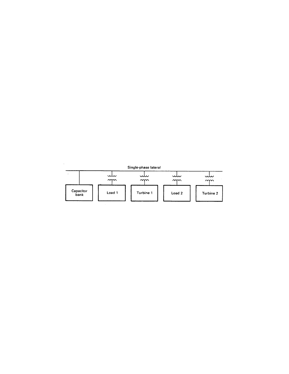
Chapter 5—Electrical Network
5–55
equate to meet load, with generators and transmission lines turning off in a domino fashion.
Emergency control action is necessary in this state to keep as much of the system as possible
from collapse.
In the restorative state, control action is taken to pick up lost load and reconnect the
system. This can easily take several hours to accomplish.
System disintegration may result in wind generators operating in an island. A simple
island, consisting of two wind turbines, two loads, and a capacitor bank used for voltage
control in the normal state, is shown in Fig. 29. If the wind turbines are using induction
generators, there is a good possibility that these generators will draw reactive power from the
capacitor bank and will continue to supply real power to the loads. This can be a planned
method of operating a turbine independently of the utility system, as we shall see in the next
chapter. Without the proper control system, however, the voltage and frequency of the island
may be far away from acceptable values. Overvoltage operation may damage much of the load
equipment as well as the induction generators themselves. Frequencies well above rated can
destroy motors by overspeed operation. Under frequency operation may also damage motors
and loads with speed sensitive oiling systems, including many air conditioning systems.
Figure 29: Electrical island.
In addition to the potential equipment problems, there is also a safety hazard to the utility
linemen. They may think this particular section of line is dead when in fact it is quite alive. In
fact, because of the self-excitation capability of the induction generator, the line may change
from dead to live while the linemen are working on it, if the wind turbines are not placed in
a stop mode.
All of these problems can be handled by proper system design and proper operating pro-
cedures, but certain changes in past operating procedures will be necessary. In the past, the
control, monitoring, and protection functions at a distribution substation have generally been
performed by separate and independent devices. Information transfer back to the dispatch
center was very minimal. Trouble would be discovered by customer complaints or by util-
ity service personnel on a regular maintenance and inspection visit to the substation. An
increasing trend is to install SCADA systems at the substations and even to extend these
systems to the individual customer. A SCADA system will provide status information to the
dispatcher and allow him to make necessary adjustments to the distribution system. At the
customer level, the SCADA system can read the meter and control interruptible loads such
Wind Energy Systems by Dr. Gary L. Johnson
November 21, 2001

Chapter 5—Electrical Network
5–56
as hot water heaters. Once the SCADA system is in place, it is a relatively small incremental
step to measure the voltage at several points along a feeder and adjust the voltage regulator
accordingly. This should minimize the effect of wind generators on the distribution lines.
At the next level of control, the larger wind electric generators will have their own computer
control system. This computer could be intertied with the SCADA system so the utility
dispatcher would know the wind generator’s power production on a periodic basis. It would
be desirable for the dispatcher to be able to shut the wind turbine down if a severe storm was
approaching the turbine, for example. It would also be desirable for the dispatcher to be able
to shut the turbine down in emergency situations such as islanding. There may also be times
when the utility cannot effectively use the wind power produced that the dispatcher would
also want to turn the turbine off. This would normally occur late at night when the electrical
demand is at its minimum and the large steam turbine generators on the utility system have
reached their minimum power operating point. The large generators will be needed again in a
few hours but have to operate above some minimum power in the meantime. Otherwise they
have to be shut down and restarted, a potentially long and expensive operation. It would be
more economical for the utility to shut down a few wind turbines for a couple of hours than
to shut down one of their large steam units.
The division of computer functions between the dispatch center and a wind turbine presents
a challenge to the design engineer. As much local control as possible should be planned at the
wind turbine, to improve reliability and reduce communication requirements. One possible
division of local and dispatcher control is shown in Table 5.3. At the wind turbine is the
capability to sense wind conditions, start the turbine, shut it down in high winds, synchronize
with the utility grid, and perhaps to deliver acceptable quality power to an electrical island or
an asynchronous load. There are also sensors and a communication link to supply information
to the dispatch center on such things as operating mode (is the turbine on or off?), power
flow, voltage magnitude, and the total energy production for revenue metering purposes. The
dispatch center will examine these parameters on a regular basis, perhaps once an hour, and
also immediately upon receipt of an alarm indication. The dispatch center may also be able to
turn the turbine on or off, or even to change the power level of a sophisticated variable-pitch
turbine.
The benefits of such two-way communication and control can be significant. It can improve
system reliability. It can also improve operating economics. It may even be able to control
operation of electrical islands. Certainly, it will help to reduce equipment losses from system
faults, and to improve the safety of maintenance operations.
The costs can also be quite significant. A utility considering a new distribution dispatch
center can expect the building, interfaces, displays, information processors, and memory to
an installed cost of at least $700,000 in 1978 dollars[2]. A FM communications tower which
can service an area of 30 to 40 km in radius would cost another $50,000. At each wind
generator, the cost of communications equipment, sensors, and control circuitry could easily
exceed $10,000. This does not include the circuit breakers and other power wiring.
Wind Energy Systems by Dr. Gary L. Johnson
November 21, 2001

Chapter 5—Electrical Network
5–57
TABLE 5.3 Communication and Control
between a Large Wind Turbine Generator
and a Dispatch Center
Under Local Control
(a) Start Capability
(b) Synchronization
(c) Stand-Alone Capability
(d) Protection
Information to Dispatch Center
(a) Operating Mode (on/off)
(b) Power Flow
(c) Voltage Magnitude
(d) Revenue Metering
Control from Dispatch Center
(a) Change Operating Mode
(b) Change Power Level
If there were 75 wind turbines being monitored and controlled by the dispatch center,
and all the dispatch center costs were to be allocated to them, each wind turbine would be
responsible for $10,000 of equipment at the dispatch center and another $10,000 of equipment
at the turbine. This $20,000 would present a major obstacle to the purchase of a 5 kW wind
generator priced at $8000, but not nearly as much of an obstacle to a 2.5 MW wind generator
priced at $2,000,000. In one case the monitoring and control equipment cost 2.5 times as
much as the wind generator itself, and only 1 percent of the wind generator cost in the second
case. This is another economy of scale for wind generators. In addition to turbine cost per
unit area decreasing with size, and power output per unit area increasing with size because of
greater height and therefore better wind speeds, the cost of monitoring and control per unit
area also decreases with turbine size.
The probable result of these economic factors is that small wind generators, less than
perhaps 20 kW maximum power rating, will not be monitored and controlled by a dispatch
center. Each small wind generator will have its own start, stop, and protective systems. The
utility will somehow assure itself that voltage magnitudes are within acceptable limits and
that electrical islands cannot operate on wind power alone and continue to operate the system
in a manner much like the past. This should be satisfactory as long as the total installed wind
generator capacity is significantly less than the minimum load on a feeder line.
On the other hand, large wind turbines will almost certainly be monitored and controlled
by the appropriate dispatch center. This control can result in significant benefits to both the
utility and the wind turbine, with acceptable costs.
Wind Energy Systems by Dr. Gary L. Johnson
November 21, 2001
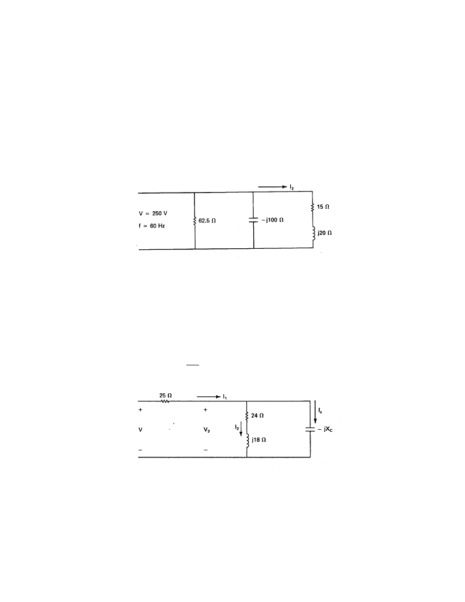
Chapter 5—Electrical Network
5–58
9 PROBLEMS
1. In the circuit of Fig. 30, the applied single-phase voltage is 250 V and the frequency is
60 Hz. The magnitude of the current in the series RL branch is |I
2
| = 10 A.
(a) What is the real power supplied to the circuit?
(b) What is the net reactive power supplied to the circuit? Is it positive or negative?
(c) What is the power factor of the circuit and is it leading or lagging?
Figure 30: Circuit diagram for Problem 1.
2. In the circuit of Fig. 31, a total real power of 4000 W is being supplied to the single-phase
circuit. The input current magnitude is
|I
1
| = 8 A.
(a) Find
|I
2
|.
(b) Find
|V
2
|.
(c) Assume that V
2
=
|V
2
|/0
o
and draw V
2
, I
2
, I
c
, and I
1
on a phasor diagram.
(d) Determine X
C
.
Figure 31: Circuit diagram for Problem 2.
3. A load connected across a single-phase 240-V, 60-Hz source draws 10 kW at a lagging
power factor of 0.5. Determine the current and the reactive power.
Wind Energy Systems by Dr. Gary L. Johnson
November 21, 2001
Chapter 5—Electrical Network
5–59
4. A small industry has a number of induction motors which require a total apparent power
of 100 kVA at a lagging power factor of 0.6. It also has 20 kW of resistance heating.
What is the total apparent power required by the industry and what is the overall power
factor?
5. A single-phase generator supplies a voltage E to the input of a transmission line repre-
sented by a series impedance Z
t
= 1 + j3 Ω. The load voltage V is 250 /0
o
V. The
circuit is shown in Fig. 32.
(a) With switch S
1
open, calculate the current I
1
, and the real power, reactive power,
and power factor of the load.
(b) Calculate the generator voltage E.
(c) Calculate the power lost in the transmission line.
(d) With switch S
1
closed and the voltage V remaining at 250/0
o
, find the capacitor
current I
c
, the new input current I
1
, and the new overall power factor.
(e) Calculate the new generator voltage and the new transmission line power loss.
(f) List two advantages of adding a capacitor to an inductive load.
Figure 32: Circuit diagram for Problem 5.
6. A three-phase load draws 250 kW at a power factor of 0.707 lagging from a 440-V line.
In parallel with this load is a three-phase capacitor bank which draws 60 kVA. Find the
magnitude of the line current and the overall power factor.
7. A wind turbine of the same rating as the MOD-1 has a synchronous generator rated at
2000 kW (2500 kVA at 0.8 power factor) at 4160 V line to line. The machine impedance
is 0.11 + j10Ω/phase. The generator is delivering 1500 kW to a load at 0.9 power factor
lagging. Find the phasor current, the phasor generated voltage E, the power angle δ,
the total pullout power, and the ohmic losses in the generator stator.
8. The field supply for the machine in the previous problem loses a diode. This causes
|E|
to decrease by 10 percent. Real power being delivered to the utility grid is determined
by the wind power input and does not change. What is the new power angle δ and the
new total reactive power being supplied to the utility grid?
Wind Energy Systems by Dr. Gary L. Johnson
November 21, 2001

Chapter 5—Electrical Network
5–60
9. A 500-kW Darrieus wind turbine is equipped with a synchronous generator rated at 480
V line to line and 625 kVA at 0.8 power factor. Rated current is flowing and the current
leads the voltage by 40
o
. What are the real and reactive powers being supplied to the
load?
10. A MOD-OA generator is rated at 250 kVA, 60 Hz, and 480 V line to line. It is connected
in wye and each phase is modeled by a generated voltage E in series with a synchronous
reactance X
s
. The per unit reactance is 1.38. What is the actual reactance per phase?
What is the actual inductance per phase?
11. The generator in the previous problem is connected to a circuit with a chosen base of
1000 kVA and 460 V. Find the per unit reactance on the new base.
12. A three-phase induction generator is rated at 230 V line to line and 14.4 A at 60 Hz.
Find the base impedance, the base inductance, and the base capacitance.
13. A 11.2-kW (15 hp), 220-V, three-phase, 60-Hz, six-pole, wye-connected induction motor
has the following parameters per phase: R
1
= 0.126 Ω, R
2
= 0.094 Ω, X
1
= X
2
= 0.248
Ω, R
m
= 92 Ω, and X
m
= 8 Ω. The rotational losses are accounted for in R
m
. The
machine is connected to a source of rated voltage. For a slip of 2.5 percent find:
(a) The line current and power factor.
(b) The power output in both kW and hp.
(c) The starting torque (s = 1.0).
14. A three-phase, 440-V, 60-Hz, eight-pole, wye-connected, 75-kW (100-hp) induction mo-
tor has the following parameters per phase: R
1
= 0.070 Ω, R
2
= 0.068 Ω, X
1
= X
2
= 0.36 Ω, R
m
= 57 Ω, and X
m
= 8.47 Ω. For a slip of 0.03 determine the input line
current, the power factor, and the efficiency.
15. A three-phase, 300-kW (400-hp), 2000-V, six-pole, 60-Hz, wye connected squirrel-cage
induction motor has the following parameters per phase that are applicable at normal
slips: R
1
= 0.200 Ω, X
1
= X
2
= 0.707 Ω, R
2
= 0.203 Ω, X
m
= 77 Ω, and R
m
= 308 Ω.
For a slip of 0.015 determine the input line current, the power factor, the torque, and
the efficiency.
16. The induction machine of the previous problem is operated as a generator at a slip of
−0.017. Find I
1
, I
2
, input mechanical power, real and reactive power, and the efficiency.
Comment on any overload.
17. An autotransformer is connected to the motor of problem 7 for starting. The motor
voltage is reduced to 0.7 of its rated value. Find the motor starting current, the line
current at start, and the starting torque. Note that s = 1 at start.
18. The model utility system of Fig. 22 implements a massive conservation and load man-
agement program which reduces the daily peak load an average of 700 MW. Compute
the new annual risk R
a
, assuming the same 7000 MW of generation as in Fig. 22.
Wind Energy Systems by Dr. Gary L. Johnson
November 21, 2001

Chapter 5—Electrical Network
5–61
References
[1] Chestnut, Harold and Robert L. Linden: Monitoring and Control Requirement Definition
Study for Dispersed Storage and Generation (DSG), General Electric Company Corporate
Research and Development Report DOE/JPL 955456-1, Volume 1, October, 1980.
[2] Chestnut, Harold and Robert L. Linden: Monitoring and Control Requirement Definition
Study for Dispersed Storage and Generation (DSG), General Electric Company Corporate
Research and Development Report DOE/JPL 955456-1, Volume 5, October, 1980.
[3] Garver, L. L.: “Effective Load Carrying Capability of Generating Units”, IEEE Trans-
actions on Power Apparatus and Systems, Vol. PAS-85, No. 8, August, 1966.
[4] Jorgensen, G. E., M. Lotker, R. C. Meier, and D. Brierley: “Design, Economic and
System Considerations of Large Wind-Driven Generators”, IEEE Transactions on Power
Apparatus and Systems, Vol. PAS-95, No. 3, May/June 1976, pp. 870-878.
[5] Marsh, W.D.: Requirements Assessment of Wind Power Plants in Electric Utility Sys-
tems, Vol. 2, EPRI Report ER-978, January, 1979.
[6] Odette, D. R.: A Survey of the Wind Energy Potential of Kansas, M.S. thesis, Electrical
Engineering Department, Kansas State University, Manhattan, Kans., 1976.
[7] Ramakumar, R., H. J. Allison, and W. L. Hughes: “Solar Energy Conversion and Storage
Systems for the Future”, IEEE Transactions on Power Apparatus and Systems, Vol. PAS-
94, No. 6, Nov./Dec. 1975, pp. 1926-1934.
[8] Seidel, R. C., H. Gold, and L. M. Wenzel: Power Train Analysis for the DOE/NASA
100-kW Wind Turbine Generator, DOE/NASA/1028-78/19, NASA TM-78997, October
1978.
Wind Energy Systems by Dr. Gary L. Johnson
November 21, 2001
Wyszukiwarka
Podobne podstrony:
[2006] Application of Magnetic Energy Recovery Switch (MERS) to Improve Output Power of Wind Turbine
Innovative Solutions In Power Electronics For Variable Speed Wind Turbines
How I built an electricity producing wind turbine
Wind Turbine and Grid Connection Modelling with PSCAD
piggott how to build a wind turbine
[Engineering] Electrical Power and Energy Systems 1999 21 Dynamics Of Diesel And Wind Turbine Gene
[2006] Application of Magnetic Energy Recovery Switch (MERS) to Improve Output Power of Wind Turbine
Tesla Wind Turbine Grid Connection And Interaction
[2001] State of the Art of Variable Speed Wind turbines
3 Wind Turbine PL
CEI 61400 22 Wind turbine generator systems Required Design Documentation
Inverter controller for HVDC systems connected to weak AC sy
1801 Design Analysis of Fixed Pitch Straight Bladed Vertical Axis Wind Turbines
DIY 1000 watt wind turbine id 1 Nieznany
Darrieus Wind Turbine Design, Construction And Testing
20060028025 Wind Turbine Generator System
więcej podobnych podstron