
1
Journal of Theoretics
Redshift Calculations in the
Dynamic Theory of Gravity
Ioannis Iraklis Haranas
Department of Physics and Astronomy
York University
128 Petrie Science Building
York University
Toronto – Ontario
CANADA
E
mail:
ioannis@yorku.ca
Abstract:
In a new theory called Dynamic Theory of Gravity, the cosmological
distance to an object and also its gravitational potential can be calculated.
We first measure its redshift on the surface of the Earth. The theory can be
applied as well to an object in orbit above the Earth, e.g., a satellite such as
the Hubble telescope. In this paper, we give various expressions for the
redshifts calculated on the surface of the Earth as well as on an object in orbit,
being the Hubble telescope. Our calculations will assume that the emitting
body is a star of mass M = M
X-ray(source)
= 1.6×10
8
M
solar masses
and a core radius R
= 80 pc, at a cosmological distance away from the Earth. We take the orbital
height h of the Hubble telescope to be 450 Km.
Introduction:
There is a new theory of gravity called Dynamic Theory of Gravity
[DTG]. Based on classical thermodynamics Ref:[1] [2] [3] [9] it has been shown
that the fundamental laws of Classical Thermodynamics also require Einstein’s

2
postulate of a constant speed of light. DTG describes physical phenomena in
terms of five dimensions: space, time, and mass. Ref[4] The theory makes its
predictions for redshifts by working in the five dimensional geometry of space,
time, and mass, and determines the unit of action in the atomic states in a
way that can be calculated with the help of quantum Poisson brackets when
covariant differentiation is used:
[
]
[ ]
{
}
Φ
Γ
+
=
Φ
,
,
q
s
q
s
q
x
g
i
p
x
µ
µ
ν
ν
µ
δ
=
.
(1)
In (1) the vector curvature is contained in the Chrisoffel symbols of the
second kind and the gauge function Φ is a multiplicative factor in the metric
tensor g
ν
q
, where the indices take the values ν, q = 0,1,2,3,4. In the
commutator, x
µ
and p
ν
are the space and momentum variables respectively,
and finally δ
µ
q is the Cronecker delta. In DTG the momentum ascribed as a
variable canonically conjugated to the mass is the rate at which mass may be
converted into energy. The canonical momentum is defined as follows below:
,
(1a)
4
4
mv
p
=
where the velocity in the fifth dimension is given by:
D
α
γ
•
=
4
v
,
(1b)
and is a time derivative where gamma itself has units of mass density or
kg/m
•
γ
3
, and α
o
is a density gradient with units of kg/m
4
. In the absence of
curvature, (1) becomes:
[
]
Φ
=
Φ
,
q
ν
ν
µ
δ
=
i
p
x
.
(2)

3
From (2) we see that the unit of action is the product of a multiple of
Cronecker’s δ
µ
q function and the gauge function Φ. It can be also shown that
if we use gauge field equations Ref:[6] then the gauge function Φ is of the
form:
(
)
−
+
=
Φ
R
R
Bt
A
k
λ
exp
exp
.
(3)
Assuming conservation of photon energy and expanding the
exponentials and then comparing this expression with (11), we need then to
evaluate the constants A, B, and k. Recalling that the emission time t
e
= 0 and
the received time t
r
= L /c, the expression for the redshift reduces to the
following: Ref[5]
1
exp
2
e
−
+
−
−
=
∆
=
−
⊕
⊕
−
−
r
r
em
em
ob
ob
R
ob
ob
em
R
e
ob
R
r
e
R
M
R
M
c
HL
R
e
M
R
e
M
c
G
z
λ
λ
λ
λ
λ
,
(4)
where
⊕
⊕
R
M
is the gravitational potential of the earth,
ob
ob
R
M
is the
reduced gravitational potential at the detection point, and
em
em
R
M
is at the
emission point of the radiation. Since λ << R, expression (4) can be simplified
for the earth’s surface (Es): Ref [5].

4
[
]
+
−
−
=
+
c
HL
R
M
R
M
c
G
z
em
em
ob
ob
Es
2
1
ln
,
(5)
and for orbiting Hubble telescope (ht) of a height h the following expression:
[
]
(
)
+
+
−
+
−
=
+
⊕
⊕
⊕
⊕
h
R
R
c
HL
R
M
h
R
M
c
G
z
em
em
ht
2
1
ln
.
(6)
As a result of the analysis in Ref[5], we solve two equations with two
unknowns, the gravitational potential GM/R and the cosmological distance L
of the emitting object. These can be found from:
[
]
[
+
+
−
+
+
=
⊕
⊕
⊕
Es
ht
z
h
R
R
z
h
R
c
R
GM
1
ln
1
ln
1
2
]
(7)
and
[
]
(
)
+
+
+
−
+
=
⊕
⊕
⊕
R
c
GM
h
R
z
z
H
c
L
ht
Es
2
1
]
1
ln[
1
ln
.(8)
In this theory, the predicted redshifts are significantly different when
measured on the surface of the Earth, or at a height of 450 km for example
above the surface. In Einstein’s theory of relativity, the redshift of an object
may be written as follows:
−
−
=
em
em
ob
ob
R
M
R
M
c
G
z
2
,
(9

5
where the subscripts specify the emitter and observer gravitational
potentials respectively. Since the redshift of an object at cosmological distance
L is given by:
L
c
H
z
=
,
(10)
then the total redshift will be given from: Ref[4]
L
c
H
R
M
R
M
c
G
z
em
em
ob
ob
+
−
−
=
2
,
(11)
where H is Hubble’s constant, c is the speed of light, and L the cosmological
distance to the object. Any difference in the redshift will come from the
difference between the gravitational potential at the surface of the earth and
at some height above the surface. However, this difference will be small due
to the small size of the earth compared with cosmological objects. Compared
with the Sun, this effect would be of the order of 10
-5
. In the case z
Es
≈ z
ht
(7)
and (8) simplify as follows:
[
1
ln
2
Es
em
em
z
c
R
GM
+
=
]
,
(11a)
=
⊕
⊕
2
R
GM
c
H
c
L
.
(11b)

6
Let us now proceed by writing the two fudamental relations predicted by
the DTG in terms of emitted λ
em
and observed λ
ob
. Since
1
−
=
em
ob
z
λ
λ
we
obtain:
+
−
+
=
⊕
⊕
⊕
m
e
ob
Es
em
ob
ht
em
em
h
R
R
h
R
c
R
GM
λ
λ
λ
λ
)
(
)
(
2
ln
ln
1
, (12)
and
+
+
=
⊕
⊕
⊕
2
)
(
)
(
1
ln
c
R
GM
h
R
H
c
L
ob
ht
ob
Es
λ
λ
.
(13)
Solving (13) for the wavelength of the radiation as observed by the
Hubble telescope we have:
−
+
−
=
⊕
⊕
⊕
2
)
(
)
(
exp
c
R
GM
c
LH
h
R
h
ob
Es
ob
ht
λ
λ
.
(14)
At the earth’s surface the wavelength of the observed radiation has the
value of:
−
+
=
⊕
⊕
⊕
2
)
(
)
(
xp
e
c
R
GM
c
LH
h
R
h
ob
ht
ob
Es
λ
λ
.
(15)

7
Similarly, we can find identical expressions as described above for the
quantities in terms of an orbital height h, cosmological redshift z, and Earth’s
gravitational potential at height h. Thus from (12) we have:
[
]
[ ]
−
=
⊕
−
+
⊕
⊕
R
h
c
R
GM
e
e
R
h
em
R
h
ob
ht
ob
Es
2
1
)
(
)
(
exp
λ
λ
λ
(16)
and
+
+
+
=
⊕
⊕
⊕
em
ob
Es
em
em
em
ob
ht
h
R
R
c
R
GM
R
h
h
λ
λ
λ
λ
)
(
2
)
(
ln
exp
.
(17)
Calculating the Redshift Expressions:
For all the expressions above, we now use: mass of the earth
M =5.97×10
⊕
24
kg, h=450 km, R
= 6.378×10
ob
6
m, and z
tot
=4.4. This
perticular redshift is associated with the X-ray source 4U0241+61 which has a
mass M
source
= 1.6×10
8
M
solar
. An object of such redshift will be at a distance:
Ref[7]
(
)
[
]
years
light
10
203
.
9
z
1
-
1
10
9
5
.
1
10
×
=
+
=
−
object
d
(17a)
From (13) and (12) we obtain the following relationships for the
wavelengths at the earth’s surface and at the Hubble telescope:
Es(ob)
)
(
0.750
λ
λ
≅
ob
ht
(18)

8
)
(
)
(
336
.
1
ob
ht
ob
Es
λ
λ
≅
.
(19)
Next, we calculate the same wavelengths with a main contribution due
to the quasar’s gravitational potential as well as the emitted and observed
wavelengths, radius of the earth, and height above of the earth’s surface.
[
]
[ ]
0705
.
0
0705
.
1
ht(obs)
)
(
999
.
0
−
≅
em
ob
Es
λ
λ
λ
(20)
em
)
(
832
.
4
λ
λ
≅
ob
ht
.
(21)
We see that (20) and (21) also contain the emitted wavelength since it
appears in the analytical solution for λ
ht
and λ
Es
. Let us now choose the
commonly occuring Lyman ( L
α
) line in quasar spectra, having an emitted
wavelength λ
em
= 1216
D
A
. If the quasar’s redshift z
tot
= 4.4, then standard
theory predicts that this line would be redshifted by a factor (1+z
tot
) λ giving
6566
D
A
: Ref[8] Next we find the following results:
(23)
%
0.19
of
e
%differenc
A
6579
A
4924
A
6566
Es
)
(
)
(
)
(Re
=
=
=
=
λ
λ
λ
λ
D
D
D
obs
Dyna
Es
obs
ht
l
Es
obs
Next, using (22) we obtain:

9
(24)
%
01
.
0
difference
%
A
6565
A
5875
A
6566
Es
)
(
)
(
)
(Re
−
=
=
=
=
λ
λ
λ
λ
D
D
D
obs
obs
Dyna
Es
obs
ht
l
Es
Calculation of the Dynamical Redshifts
Given the total redshift of the quasar z
tot
= 4.4 we can obtain and solve
the system of equations which DTG claims for the dynamical redshifts on the
earth and at the height of the Hubble telescope. Using the distance to the
quasar as given in (17a) and taking its mass to be M
X—Ray Quasar
= 1.6×10
8
M
Solar-
Masses
= 3.04×10
38
kg, we need to solve the system of the following equations:
(
)
(
)
[
]
(
)
(
)
[
]
[
]
0
10
937
.
6
1
ln
1
ln
173
.
15
491
.
0
0
1
ln
934
.
0
1
ln
173
.
15
10
841
.
5
10
4
=
×
+
+
−
+
−
=
+
−
+
−
×
−
−
ht
Es
Es
ht
z
z
z
z
(25)
from which we obtain the percent change of redshift:
(26)
%,
089
.
1
%
052
.
0
%
635
.
0
%
583
.
0
ht
Es
Es
ht
z
z
z
z
z
=
=
∆
=
=
If we take the value of z
ES
= 4.4 we find that:

10
(27)
%
359
.
0
%
040
.
4
%
400
.
4
=
∆
=
=
z
z
z
ht
Es
Dynamical Redshift Equations
If we now allow the potential due to the emitting body to change in
general by a factor A, in the system of equations in (25) then we can write
two solutions for z
in the following form:
Es
ht
z
and
[
]
[
1
e
583
.
1
1
e
635
.
1
5
-
-5
10
1.769
10
1.769
−
=
−
=
×
×
A
ht
A
Es
z
z
]
(28)
or in-terms of the emitted wavelength we have:
(29)
.
583
.
1
635
.
1
5
5
10
769
.
1
10
769
.
1
em
Es
A
em
ht
A
e
e
−
−
×
×
=
=
λ
λ
λ
λ
Simirarly, we can obtain the dynamical redshifts at the surface of the
earth and at the height of the Hubble telescope if we allow for the
cosmological redshift to change ( smaller or larger ) by a factor B. Thus we
obtain:
(30)
1
e
000
.
1
1
000
.
1
0.491824B
459407
.
0
−
=
−
=
Es
B
ht
z
e
z

11
which in-terms of the emitted wavelength becomes:
(31)
.
000
.
1
000
.
1
491824
.
0
em
Es
459407
.
0
em
B
B
ht
e
e
λ
λ
λ
λ
=
=
To obtain a dynamical redshifts or dynamical wavelengths at the surface
of the earth or at the Hubble telescope our constants A and B should in
general have the following values:
( )
(
)
[
]
( )
(
)
[
]
(
)
(
)
=
=
+
=
+
=
em
Es
ht
em
Es
Es
631
.
0
ln
56529
611
.
0
ln
56529
1
631
.
0
ln
56529
1
4
.
0
611
.
0
ln
56529
λ
λ
λ
λ
λ
λ
A
A
z
z
A
z
z
A
ht
ht
Es
Es
(31a)
also
( )
(
)
[
]
( )
(
)
[
]
(
)
(
)
=
=
+
=
+
=
em
ht
ht
em
Es
Es
999
.
0
ln
176
.
2
999
.
0
ln
033
.
2
1
999
.
0
ln
033
.
2
1
999
.
0
ln
033
.
2
λ
λ
λ
λ
λ
λ
B
B
z
z
B
z
z
B
ht
ht
Es
Es
(31b)
12
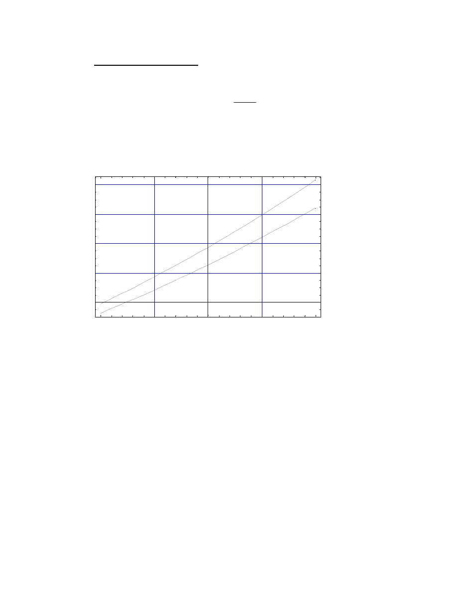
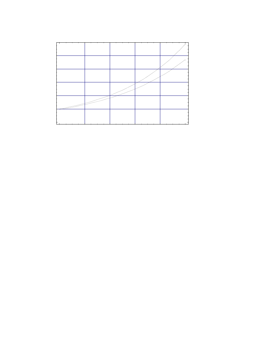
Plotting the Equations
To plot equations (28) and (29) we let A take some values below and
above relative to
2
)
(
c
R
GM
quasar
z
e
e
nal
gravitatio
=
and we obtain the following
graphs in Figure 1 and 2
z
Es
,z
ht
0
5000
10000
15000
20000
2000
2200
2400
2600
2800
9
Dynamical Redshifts
H
Z
ES
Z
HT
L
vs A
H
GM
e
€€€€€€€€€€€€
R
e
c
2
L
=
A (G M
e
/ R
e
c
2
)
Figure:1 Plots of Dynamical Redshifts at the Earth’s Surface
and at Hubble Telescope versus Quasars’s Gravitational Redshift
Factor.
λ
Es
,λ
ht
13
0
20000
40000
60000
80000
100000
0
2000
4000
6000
8000
10000
9
Dynamical Wavelengths
H
l
ES
l
HT
L
vs A
H
GM
e
€€€€€€€€€€€€
R
e
c
2
L
=
A (G M
e
/ R
e
c
2
)
Figure:2 Plots of Dynamical Wavelengths at the Earth’s Surface
and at Hubble Telescope versus Quasars’s Gravitational Redshift
Factor.
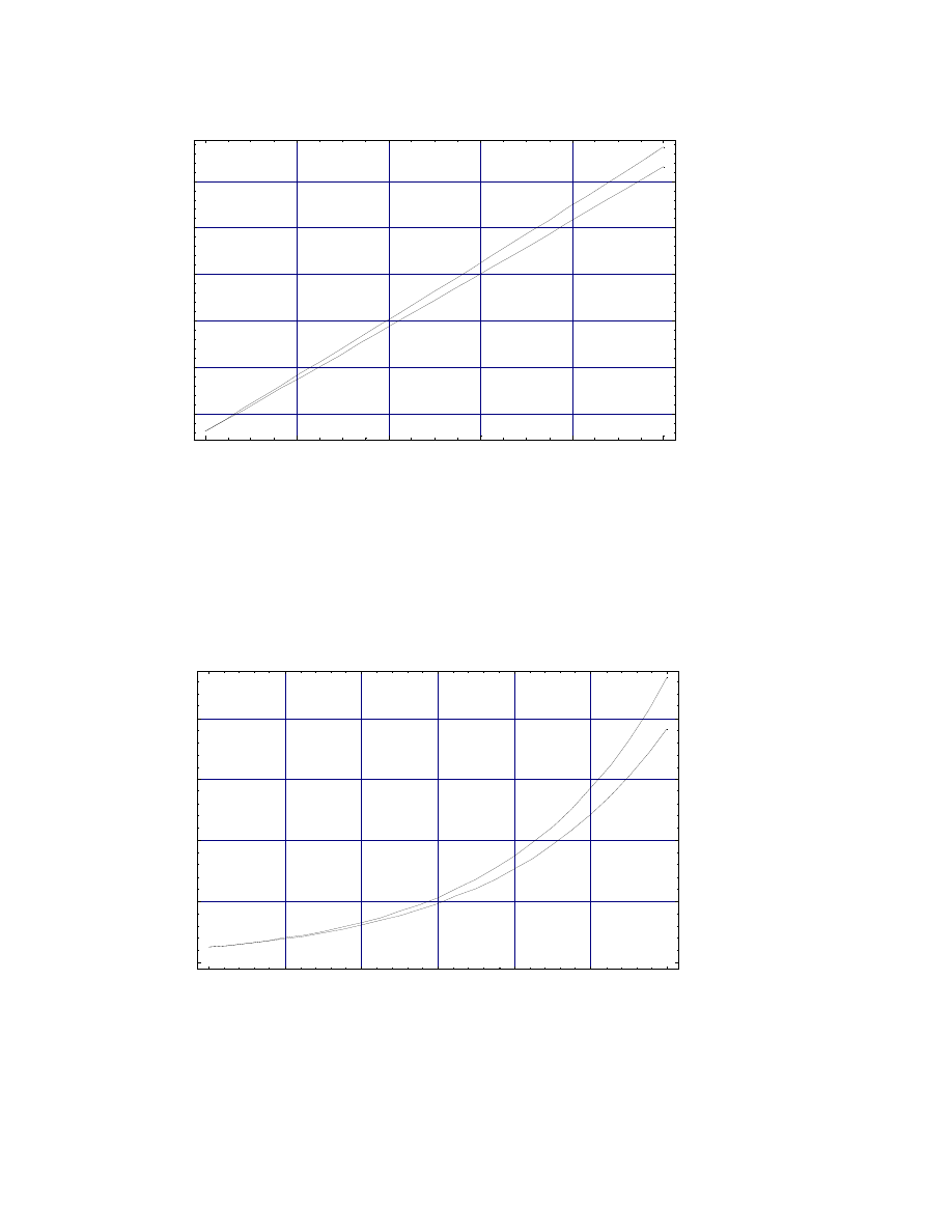
Similarly for the equations (30) and (31) containing B we obtain two graphs in
figures 3 and 4:
z
Es
,z
ht
14
0
0.02
0.04
0.06
0.08
0.1
1220
1230
1240
1250
1260
1270
9
Dynamical Redshifts
H
Z
ES
Z
HT
L
vs B
H
HL
€€€€€€€
c
L
B(LH/c)
Fig:3 Plot of Dynamical Redshifts at Earths Surface and
Hubble versus Cosmological Redshift Factor.
λ
Es
,λ
ht
0
1
2
3
4
5
6
0
5000
10000
15000
20000
9
Dynamical Wavelengths
H
l
ES
l
HT
L
vs B
H
HL
€€€€€€€
c
L
B(LH/c)

15
Fig: 4 Plots of Dynamical Wavelengths at the Earth’s Surface
and at Hubble Telescope versus Quasars’s Gravitational Redshift
Factor.
Conclusions:
In this paper, we have highlighted a few aspects of the dynamic theory
of gravity. Analytical expressions were obtained for the observed wavelengths
on the earth’s surface and for an orbital height h given the gravitational
potential, the cosmological distance, and the redshift factor. Finally, all these
expressions for the wavelengths on the earth’s surface, as well as at the height
of the Hubble telescope, were calculated for a particular quasistellar object of
mass M
X-ray(source)
= 1.6×10
8
M
solar masses
and radius R = 80 pc.
We see that, in the dynamic theory of gravity those equations which
describe the values of the wavelength-change at the earth’s surface, and at
the height of the Hubble telescope, produce changes relative to the original
wavelength. For the observer, the light emitted from the quasar on the earth
will be slightly redder in this theory than in the relativistic one. The same
wavelengths will also be redder w.r.t the Hubble telescope observed
wavelength. There is a 0.19 % percentage difference between the DTG and
the total relativistic prediction at height h above the surface of the earth, when
the total redshift is the sum of relativistic and cosmological. It seems that at
the Hubble height the wavelength observed will be 1.336 times less than that
from DTG on the earth’s surface.
When the observed wavelength at the surface of the earth and at
Hubble are given interms of the gravitational potential of the quasar, and at a
height h above the earth, as well as the relativistically observed wavelength on
the earth’s surface and the emitted wavelengths, then there is a –0.01%
percentage difference between the total relativistic redshift and that which
DTG predicts. The observed wavelength at Hubble wavelength is also 1.117
times less than that observed at the surface of the earth.

16
Next, solving the system of two equations in two unknowns for the
same quasar, the percent changes of the redshifts at the earth’s surface and at
Hubble were calculated, and from there the actual z values. A percentage
difference of
–8.18% was found, and also a ∆z = 0.359 between the two values of z
ES
and
z
HT
.
Finally, general solutions of z’s and λ’s were obtained in-terms of A and
B being some multiple or submultiple values of gravitational and cosmological
redshift, and then plotted. For very large values of A and B, the DTG redshifts
and wavelengths seem to diverge, whereas at small values of A and B, they
both follow a linear behaviour that seems to converge to each-other at A = 0
and
B =0. This could mean that there is no distinction between DTG and
relativistic gravitational effects when A and B are very small. The effects
become distinct at larger values of A and B as shown by the graphs. Here it
may be resonable to assume that objects of large redshift and potential might
be canditates in detecting DTG effects.
References
[1] P. E. Williams, “ On a Possible Formulation of Particle Dynamics in Terms
of Thermodynamic Conceptualizations and the Role of Entropy in it.”
Thesis U.S. Naval Postgraduate School, 1976.
[2] P.E. Williams, “The Principles of the Dynamic Theory” Research Report
EW-77-4, U.S. Naval Academy, 1977.
[3] P. E. Williams, “The Dynamic Theory: A New View of Space, Time, and
Matter”, Los Alamos Scientific Laboratory report LA-8370-MS, Feb 1980.
[4] P. E. Williams, “ Quantum Measurement, Gravitation, and Locality in the
Dynamic Theory”, Symposium on Causality and Locality in Modern Physics

17
and Astronomy: Open Questions and Possible Solutions, York University,
North York, Canada, August 25-29, 1997.
[5] P. E. Williams, Using the Hubble Telescope to Determine the Split of a
Cosmological Object’s Redshift into its Gravitational and Distance Parts,
Apeiron, Vol. 8, No. 2, April 2001.
[6] P. E. Williams, The Dynamic Theory: A New View of Space-Time –Matter,
1993,
http:// www.nmt.edu/~pharis/
[7]
Science Journal, Summer 2000, Vol:17, No.1, p: 3
/ journal / sum2000 / DistObj.html
[8]
P. J. E. Peebles, Principles of Physical Cosmology, Princeton University
Press, 1993, p: 548
[9]
P. E.Williams, Mechanical Entropy and Its Implications, Entropy, 2001,
3, 76-115/
Document Outline
- Redshift Calculations in the
- Dynamic Theory of Gravity
- Ioannis Iraklis Haranas
- Abstract:
- In a new theory called Dynamic Theory of Gravity, the cosmological distance to an object and also its gravitational potential can be calculated. We first measure its redshift on the surface of the Earth. The theory can be applied as well to an object i
-
-
-
- Figure:1 Plots of Dynamical Redshifts at the Eart
- and at Hubble Telescope versus Quasars’s Gravitat
- Factor.
- Figure:2 Plots of Dynamical Wavelengths at the Ea
- and at Hubble Telescope versus Quasars’s Gravitat
- Factor.
- Fig: 4 Plots of Dynamical Wavelengths at the Eart
- and at Hubble Telescope versus Quasars’s Gravitat
- Factor.
-
- References
-
-
- Ioannis Iraklis Haranas
Wyszukiwarka
Podobne podstrony:
Haranas The Classical Problem of a Body Falling in a Tube Through the Center of the Earth in the Dy
A comparative study of inverter and line side filtering schemes in the dynamic voltage restorer
In Defense of the Representational Theory of Qualia (Replies to Neander, Rey, and Tye)
[Mises org]Raico,Ralph The Place of Religion In The Liberal Philosophy of Constant, Toqueville,
Homosexuals in the Military Analysis of the Issue
Hay The biological theory of religion
Blood in the Trenches A Memoir of the Battle of the Somme A Radclyffe Dugmore
Increased diversity of food in the first year of life may help protect against allergies (EUFIC)
Knudsen, 3rd Hand in the Angers Fragment of Saxo Grammaticus
The Contemporary Theory of Metaphor(1)
In the Key Chords of Dawn
Robert P Smith, Peter Zheutlin Riches Among the Ruins, Adventures in the Dark Corners of the Global
Holt Edward Out of many One The voice(s) in the crusade ideology of Las Navas de Tolosa Thesis final
więcej podobnych podstron