
An Introduction to Statistical
Inference and Data Analysis
Michael W. Trosset
1
April 3, 2001
1
Department of Mathematics, College of William & Mary, P.O. Box 8795,
Williamsburg, VA 23187-8795.

Contents
1 Mathematical Preliminaries
5
1.1
Sets . . . . . . . . . . . . . . . . . . . . . . . . . . . . . . . .
5
1.2
Counting . . . . . . . . . . . . . . . . . . . . . . . . . . . . .
9
1.3
Functions . . . . . . . . . . . . . . . . . . . . . . . . . . . . .
14
1.4
Limits . . . . . . . . . . . . . . . . . . . . . . . . . . . . . . .
15
1.5
Exercises
. . . . . . . . . . . . . . . . . . . . . . . . . . . . .
16
2 Probability
17
2.1
Interpretations of Probability . . . . . . . . . . . . . . . . . .
17
2.2
Axioms of Probability . . . . . . . . . . . . . . . . . . . . . .
18
2.3
Finite Sample Spaces . . . . . . . . . . . . . . . . . . . . . . .
26
2.4
Conditional Probability . . . . . . . . . . . . . . . . . . . . .
32
2.5
Random Variables . . . . . . . . . . . . . . . . . . . . . . . .
43
2.6
Exercises
. . . . . . . . . . . . . . . . . . . . . . . . . . . . .
51
3 Discrete Random Variables
55
3.1
Basic Concepts . . . . . . . . . . . . . . . . . . . . . . . . . .
55
3.2
Examples . . . . . . . . . . . . . . . . . . . . . . . . . . . . .
56
3.3
Expectation . . . . . . . . . . . . . . . . . . . . . . . . . . . .
61
3.4
Binomial Distributions . . . . . . . . . . . . . . . . . . . . . .
72
3.5
Exercises
. . . . . . . . . . . . . . . . . . . . . . . . . . . . .
77
4 Continuous Random Variables
81
4.1
A Motivating Example . . . . . . . . . . . . . . . . . . . . . .
81
4.2
Basic Concepts . . . . . . . . . . . . . . . . . . . . . . . . . .
85
4.3
Elementary Examples . . . . . . . . . . . . . . . . . . . . . .
88
4.4
Normal Distributions . . . . . . . . . . . . . . . . . . . . . . .
93
4.5
Normal Sampling Distributions . . . . . . . . . . . . . . . . .
97
1

2
CONTENTS
4.6
Exercises
. . . . . . . . . . . . . . . . . . . . . . . . . . . . . 102
5 Quantifying Population Attributes
105
5.1
Symmetry . . . . . . . . . . . . . . . . . . . . . . . . . . . . . 105
5.2
Quantiles . . . . . . . . . . . . . . . . . . . . . . . . . . . . . 107
5.2.1
The Median of a Population . . . . . . . . . . . . . . . 111
5.2.2
The Interquartile Range of a Population . . . . . . . . 112
5.3
The Method of Least Squares . . . . . . . . . . . . . . . . . . 112
5.3.1
The Mean of a Population . . . . . . . . . . . . . . . . 113
5.3.2
The Standard Deviation of a Population . . . . . . . . 114
5.4
Exercises
. . . . . . . . . . . . . . . . . . . . . . . . . . . . . 115
6 Sums and Averages of Random Variables
117
6.1
The Weak Law of Large Numbers . . . . . . . . . . . . . . . . 118
6.2
The Central Limit Theorem . . . . . . . . . . . . . . . . . . . 120
6.3
Exercises
. . . . . . . . . . . . . . . . . . . . . . . . . . . . . 127
7 Data
129
7.1
The Plug-In Principle . . . . . . . . . . . . . . . . . . . . . . 130
7.2
Plug-In Estimates of Mean and Variance . . . . . . . . . . . . 132
7.3
Plug-In Estimates of Quantiles . . . . . . . . . . . . . . . . . 134
7.3.1
Box Plots . . . . . . . . . . . . . . . . . . . . . . . . . 135
7.3.2
Normal Probability Plots . . . . . . . . . . . . . . . . 137
7.4
Density Estimates . . . . . . . . . . . . . . . . . . . . . . . . 140
7.5
Exercises
. . . . . . . . . . . . . . . . . . . . . . . . . . . . . 143
8 Inference
147
8.1
A Motivating Example . . . . . . . . . . . . . . . . . . . . . . 148
8.2
Point Estimation . . . . . . . . . . . . . . . . . . . . . . . . . 150
8.2.1
Estimating a Population Mean . . . . . . . . . . . . . 150
8.2.2
Estimating a Population Variance . . . . . . . . . . . 152
8.3
Heuristics of Hypothesis Testing . . . . . . . . . . . . . . . . 152
8.4
Testing Hypotheses About a Population Mean . . . . . . . . . 162
8.5
Set Estimation . . . . . . . . . . . . . . . . . . . . . . . . . . 170
8.6
Exercises
. . . . . . . . . . . . . . . . . . . . . . . . . . . . . 175
9 1-Sample Location Problems
179
9.1
The Normal 1-Sample Location Problem . . . . . . . . . . . . 181
9.1.1
Point Estimation . . . . . . . . . . . . . . . . . . . . . 181

CONTENTS
3
9.1.2
Hypothesis Testing . . . . . . . . . . . . . . . . . . . . 181
9.1.3
Interval Estimation . . . . . . . . . . . . . . . . . . . . 186
9.2
The General 1-Sample Location Problem . . . . . . . . . . . . 189
9.2.1
Point Estimation . . . . . . . . . . . . . . . . . . . . . 189
9.2.2
Hypothesis Testing . . . . . . . . . . . . . . . . . . . . 189
9.2.3
Interval Estimation . . . . . . . . . . . . . . . . . . . . 192
9.3
The Symmetric 1-Sample Location Problem . . . . . . . . . . 194
9.3.1
Hypothesis Testing . . . . . . . . . . . . . . . . . . . . 194
9.3.2
Point Estimation . . . . . . . . . . . . . . . . . . . . . 197
9.3.3
Interval Estimation . . . . . . . . . . . . . . . . . . . . 198
9.4
A Case Study from Neuropsychology . . . . . . . . . . . . . . 200
9.5
Exercises
. . . . . . . . . . . . . . . . . . . . . . . . . . . . . 201
10 2-Sample Location Problems
203
10.1 The Normal 2-Sample Location Problem . . . . . . . . . . . . 206
10.1.1 Known Variances . . . . . . . . . . . . . . . . . . . . . 207
10.1.2 Equal Variances . . . . . . . . . . . . . . . . . . . . . 208
10.1.3 The Normal Behrens-Fisher Problem . . . . . . . . . . 210
10.2 The 2-Sample Location Problem for a General Shift Family . 212
10.3 The Symmetric Behrens-Fisher Problem . . . . . . . . . . . . 212
10.4 Exercises
. . . . . . . . . . . . . . . . . . . . . . . . . . . . . 212
11 k-Sample Location Problems
213
11.1 The Normal k-Sample Location Problem . . . . . . . . . . . . 213
11.1.1 The Analysis of Variance . . . . . . . . . . . . . . . . 213
11.1.2 Planned Comparisons . . . . . . . . . . . . . . . . . . 218
11.1.3 Post Hoc Comparisons . . . . . . . . . . . . . . . . . . 223
11.2 The k-Sample Location Problem for a General Shift Family . 225
11.2.1 The Kruskal-Wallis Test . . . . . . . . . . . . . . . . . 225
11.3 Exercises
. . . . . . . . . . . . . . . . . . . . . . . . . . . . . 225

4
CONTENTS

Chapter 1
Mathematical Preliminaries
This chapter collects some fundamental mathematical concepts that we will
use in our study of probability and statistics. Most of these concepts should
seem familiar, although our presentation of them may be a bit more formal
than you have previously encountered. This formalism will be quite useful
as we study probability, but it will tend to recede into the background as we
progress to the study of statistics.
1.1
Sets
It is an interesting bit of trivia that “set” has the most different meanings of
any word in the English language. To describe what we mean by a set, we
suppose the existence of a designated universe of possible objects. In this
book, we will often denote the universe by S. By a set, we mean a collection
of objects with the property that each object in the universe either does or
does not belong to the collection. We will tend to denote sets by uppercase
Roman letters toward the beginning of the alphabet, e.g. A, B, C, etc.
The set of objects that do not belong to a designated set A is called the
complement of A. We will denote complements by A
c
, B
c
, C
c
, etc. The
complement of the universe is the empty set, denoted S
c
=
∅.
An object that belongs to a designated set is called an element or member
of that set. We will tend to denote elements by lower case Roman letters
and write expressions such as x
∈ A, pronounced “x is an element of the
set A.” Sets with a small number of elements are often identified by simple
enumeration, i.e. by writing down a list of elements. When we do so, we will
enclose the list in braces and separate the elements by commas or semicolons.
5

6
CHAPTER 1. MATHEMATICAL PRELIMINARIES
For example, the set of all feature films directed by Sergio Leone is
{ A Fistful of Dollars;
For a Few Dollars More;
The Good, the Bad, and the Ugly;
Once Upon a Time in the West;
Duck, You Sucker!;
Once Upon a Time in America
}
In this book, of course, we usually will be concerned with sets defined by
certain mathematical properties. Some familiar sets to which we will refer
repeatedly include:
• The set of natural numbers, N = {1, 2, 3, . . .}.
• The set of integers, Z = {. . . , −3, −2, −1, 0, 1, 2, 3, . . .}.
• The set of real numbers, < = (−∞, ∞).
If A and B are sets and each element of A is also an element of B, then
we say that A is a subset of B and write A
⊂ B. For example,
N
⊂ Z ⊂ <.
Quite often, a set A is defined to be those elements of another set B that
satisfy a specified mathematical property. In such cases, we often specify A
by writing a generic element of B to the left of a colon, the property to the
right of the colon, and enclosing this syntax in braces. For example,
A =
{x ∈ Z : x
2
< 5
} = {−2, −1, 0, 1, 2},
is pronounced “A is the set of integers x such that x
2
is less than 5.”
Given sets A and B, there are several important sets that can be con-
structed from them. The union of A and B is the set
A
∪ B = {x ∈ S : x ∈ A or x ∈ B}
and the intersection of A and B is the set
A
∩ B = {x ∈ S : x ∈ A and x ∈ B}.
Notice that unions and intersections are symmetric constructions, i.e. A
∪
B = B
∪ A and A ∩ B = B ∩ A. If A ∩ B = ∅, i.e. if A and B have no

1.1. SETS
7
elements in common, then A and B are disjoint or mutually exclusive. By
convention, the empty set is a subset of every set, so
∅ ⊂ A ∩ B ⊂ A ⊂ A ∪ B ⊂ S
and
∅ ⊂ A ∩ B ⊂ B ⊂ A ∪ B ⊂ S.
These facts are illustrated by the Venn diagram in Figure 1.1, in which sets
are qualitatively indicated by connected subsets of the plane. We will make
frequent use of Venn diagrams as we develop basic facts about probabilities.
Figure 1.1: A Venn Diagram of Two Nondisjoint Sets
It is often useful to extend the concepts of union and intersection to more
than two sets. Let
{A
α
} denote an arbitrary collection of sets. Then x ∈ S
is an element of the union of
{A
α
}, denoted
[
α
A
α
,
if and only if there exists some α
0
such that x
∈ A
α
0
. Also, x
∈ S is an
element of the intersection of
{A
α
}, denoted
\
α
A
α
,

8
CHAPTER 1. MATHEMATICAL PRELIMINARIES
if and only if x
∈ A
α
for every α. Furthermore, it will be important to
distinguish collections of sets with the following property:
Definition 1.1 A collection of sets is pairwise disjoint if and only if each
pair of sets in the collection has an empty intersection.
Unions and intersections are related to each other by two distributive
laws:
B
∩
[
α
A
α
=
[
α
(B
∩ A
α
)
and
B
∪
\
α
A
α
=
\
α
(B
∪ A
α
) .
Furthermore, unions and intersections are related to complements by De-
Morgan’s laws:
Ã
[
α
A
α
!
c
=
\
α
A
c
α
and
Ã
\
α
A
α
!
c
=
[
α
A
c
α
.
The first property states that an object is not in any of the sets in the
collection if and only if it is in the complement of each set; the second
property states that an object is not in every set in the collection if it is in
the complement of at least one set.
Finally, we consider another important set that can be constructed from
A and B.
Definition 1.2 The Cartesian product of two sets A and B, denoted A
×B,
is the set of ordered pairs whose first component is an element of A and whose
second component is an element of B, i.e.
A
× B = {(a, b) : a ∈ A, b ∈ B}.
A familiar example of this construction is the Cartesian coordinatization of
the plane,
<
2
=
< × < = {(x, y) : x, y ∈ <}.
Of course, this construction can also be extended to more than two sets, e.g.
<
3
=
{(x, y, z) : x, y, z ∈ <}.

1.2. COUNTING
9
1.2
Counting
This section is concerned with determining the number of elements in a
specified set. One of the fundamental concepts that we will exploit in our
brief study of counting is the notion of a one-to-one correspondence between
two sets. We begin by illustrating this notion with an elementary example.
Example 1
Define two sets,
A
1
=
{diamond, emerald, ruby, sapphire}
and
B =
{blue, green, red, white} .
The elements of these sets can be paired in such a way that to each element
of A
1
there is assigned a unique element of B and to each element of B there
is assigned a unique element of A
1
. Such a pairing can be accomplished in
various ways; a natural assignment is the following:
diamond
↔ white
emerald
↔ green
ruby
↔ red
sapphire
↔ blue
This assignment exemplifies a one-to-one correspondence.
Now suppose that we augment A
1
by forming
A
2
= A
1
∪ {peridot} .
Although we can still assign a color to each gemstone, we cannot do so in
such a way that each gemstone corresponds to a different color. There does
not exist a one-to-one correspondence between A
2
and B.
From Example 1, we abstract
Definition 1.3 Two sets can be placed in one-to-one correspondence if their
elements can be paired in such a way that each element of either set is asso-
ciated with a unique element of the other set.
The concept of one-to-one correspondence can then be exploited to obtain a
formal definition of a familiar concept:

10
CHAPTER 1. MATHEMATICAL PRELIMINARIES
Definition 1.4 A set A is finite if there exists a natural number N such
that the elements of A can be placed in one-to-one correspondence with the
elements of
{1, 2, . . . , N}.
If A is finite, then the natural number N that appears in Definition 1.4
is unique. It is, in fact, the number of elements in A. We will denote this
quantity, sometimes called the cardinality of A, by #(A). In Example 1
above, #(A
1
) = #(B) = 4 and #(A
2
) = 5.
The Multiplication Principle
Most of our counting arguments will rely
on a fundamental principle, which we illustrate with an example.
Example 2
Suppose that each gemstone in Example 1 has been mount-
ed on a ring. You desire to wear one of these rings on your left hand and
another on your right hand. How many ways can this be done?
First, suppose that you wear the diamond ring on your left hand. Then
there are three rings available for your right hand: emerald, ruby, sapphire.
Next, suppose that you wear the emerald ring on your left hand. Again
there are three rings available for your right hand: diamond, ruby, sapphire.
Suppose that you wear the ruby ring on your left hand. Once again there
are three rings available for your right hand: diamond, emerald, sapphire.
Finally, suppose that you wear the sapphire ring on your left hand. Once
more there are three rings available for your right hand: diamond, emerald,
ruby.
We have counted a total of 3 + 3 + 3 + 3 = 12 ways to choose a ring for
each hand. Enumerating each possibility is rather tedious, but it reveals a
useful shortcut. There are 4 ways to choose a ring for the left hand and, for
each such choice, there are three ways to choose a ring for the right hand.
Hence, there are 4
· 3 = 12 ways to choose a ring for each hand. This is an
instance of a general principle:
Suppose that two decisions are to be made and that there are n
1
possible outcomes of the first decision. If, for each outcome of
the first decision, there are n
2
possible outcomes of the second
decision, then there are n
1
n
2
possible outcomes of the pair of
decisions.

1.2. COUNTING
11
Permutations and Combinations
We now consider two more concepts
that are often employed when counting the elements of finite sets. We mo-
tivate these concepts with an example.
Example 3
A fast-food restaurant offers a single entree that comes
with a choice of 3 side dishes from a total of 15. To address the perception
that it serves only one dinner, the restaurant conceives an advertisement that
identifies each choice of side dishes as a distinct dinner. Assuming that each
entree must be accompanied by 3 distinct side dishes, e.g.
{stuffing, mashed
potatoes, green beans
} is permitted but {stuffing, stuffing, mashed potatoes}
is not, how many distinct dinners are available?
1
Answer 1
The restaurant reasons that a customer, asked to choose
3 side dishes, must first choose 1 side dish from a total of 15. There are
15 ways of making this choice. Having made it, the customer must then
choose a second side dish that is different from the first. For each choice of
the first side dish, there are 14 ways of choosing the second; hence 15
× 14
ways of choosing the pair. Finally, the customer must choose a third side
dish that is different from the first two. For each choice of the first two,
there are 13 ways of choosing the third; hence 15
× 14 × 13 ways of choosing
the triple. Accordingly, the restaurant advertises that it offers a total of
15
× 14 × 13 = 2730 possible dinners.
Answer 2
A high school math class considers the restaurant’s claim
and notes that the restaurant has counted side dishes of
{
stuffing,
mashed potatoes,
green beans
},
{
stuffing,
green beans,
mashed potatoes
},
{ mashed potatoes,
stuffing,
green beans
},
{ mashed potatoes,
green beans,
stuffing
},
{
green beans,
stuffing,
mashed potatoes
}, and
{
green beans,
mashed potatoes,
stuffing
}
as distinct dinners. Thus, the restaurant has counted dinners that differ only
with respect to the order in which the side dishes were chosen as distinct.
Reasoning that what matters is what is on one’s plate, not the order in
which the choices were made, the math class concludes that the restaurant
1
This example is based on an actual incident involving the Boston Chicken (now Boston
Market) restaurant chain and a high school math class in Denver, CO.

12
CHAPTER 1. MATHEMATICAL PRELIMINARIES
has overcounted. As illustrated above, each triple of side dishes can be
ordered in 6 ways: the first side dish can be any of 3, the second side dish
can be any of the remaining 2, and the third side dish must be the remaining
1 (3
× 2 × 1 = 6). The math class writes a letter to the restaurant, arguing
that the restaurant has overcounted by a factor of 6 and that the correct
count is 2730
÷ 6 = 455. The restaurant cheerfully agrees and donates $1000
to the high school’s math club.
From Example 3 we abstract the following definitions:
Definition 1.5 The number of permutations (ordered choices) of r objects
from n objects is
P (n, r) = n
× (n − 1) × · · · × (n − r + 1).
Definition 1.6 The number of combinations (unordered choices) of r ob-
jects from n objects is
C(n, r) = P (n, r)
÷ P (r, r).
In Example 3, the restaurant claimed that it offered P (15, 3) dinners, while
the math class argued that a more plausible count was C(15, 3). There, as
always, the distinction was made on the basis of whether the order of the
choices is or is not relevant.
Permutations and combinations are often expressed using factorial nota-
tion. Let
0! = 1
and let k be a natural number. Then the expression k!, pronounced “k
factorial” is defined recursively by the formula
k! = k
× (k − 1)!.
For example,
3! = 3
× 2! = 3 × 2 × 1! = 3 × 2 × 1 × 0! = 3 × 2 × 1 × 1 = 3 × 2 × 1 = 6.
Because
n! = n
× (n − 1) × · · · × (n − r + 1) × (n − r) × · · · × 1
= P (n, r)
× (n − r)!,

1.2. COUNTING
13
we can write
P (n, r) =
n!
(n
− r)!
and
C(n, r) = P (n, r)
÷ P (r, r) =
n!
(n
− r)!
÷
r!
(r
− r)!
=
n!
r!(n
− r)!
.
Finally, we note (and will sometimes use) the popular notation
C(n, r) =
Ã
n
r
!
,
pronounced “n choose r”.
Countability
Thus far, our study of counting has been concerned exclu-
sively with finite sets. However, our subsequent study of probability will
require us to consider sets that are not finite. Toward that end, we intro-
duce the following definitions:
Definition 1.7 A set is infinite if it is not finite.
Definition 1.8 A set is denumerable if its elements can be placed in one-
to-one correspondence with the natural numbers.
Definition 1.9 A set is countable if it is either finite or denumerable.
Definition 1.10 A set is uncountable if it is not countable.
Like Definition 1.4, Definition 1.8 depends on the notion of a one-to-one
correspondence between sets. However, whereas this notion is completely
straightforward when at least one of the sets is finite, it can be rather elu-
sive when both sets are infinite. Accordingly, we provide some examples of
denumerable sets. In each case, we superscript each element of the set in
question with the corresponding natural number.
Example 4
Consider the set of even natural numbers, which excludes
one of every two consecutive natural numbers It might seem that this set
cannot be placed in one-to-one correspondence with the natural numbers in
their entirety; however, infinite sets often possess counterintuitive properties.
Here is a correspondence that demonstrates that this set is denumerable:
2
1
, 4
2
, 6
3
, 8
4
, 10
5
, 12
6
, 14
7
, 16
8
, 18
9
, . . .

14
CHAPTER 1. MATHEMATICAL PRELIMINARIES
Example 5
Consider the set of integers. It might seem that this set,
which includes both a positive and a negative copy of each natural number,
cannot be placed in one-to-one correspondence with the natural numbers;
however, here is a correspondence that demonstrates that this set is denu-
merable:
. . . ,
−4
9
,
−3
7
,
−2
5
,
−1
3
, 0
1
, 1
2
, 2
4
, 3
6
, 4
8
, . . .
Example 6
Consider the Cartesian product of the set of natural num-
bers with itself. This set contains one copy of the entire set of natural
numbers for each natural number—surely it cannot be placed in one-to-one
correspondence with a single copy of the set of natural numbers! In fact, the
following correspondence demonstrates that this set is also denumerable:
(1, 1)
1
(1, 2)
2
(1, 3)
6
(1, 4)
7
(1, 5)
15
. . .
(2, 1)
3
(2, 2)
5
(2, 3)
8
(2, 4)
14
(2, 5)
17
. . .
(3, 1)
4
(3, 2)
9
(3, 3)
13
(3, 4)
18
(3, 5)
26
. . .
(4, 1)
10
(4, 2)
12
(4, 3)
19
(4, 4)
25
(4, 5)
32
. . .
(5, 1)
11
(5, 2)
20
(5, 3)
24
(5, 4)
33
(5, 5)
41
. . .
..
.
..
.
..
.
..
.
..
.
. ..
In light of Examples 4–6, the reader may wonder what is required to
construct a set that is not countable. We conclude this section by remarking
that the following intervals are uncountable sets, where a, b
∈ < and a < b.
(a, b) =
{x ∈ < : a < x < b}
[a, b) =
{x ∈ < : a ≤ x < b}
(a, b] =
{x ∈ < : a < x ≤ b}
[a, b] =
{x ∈ < : a ≤ x ≤ b}
We will make frequent use of such sets, often referring to (a, b) as an open
interval and [a, b] as a closed interval.
1.3
Functions
A function is a rule that assigns a unique element of a set B to each element
of another set A. A familiar example is the rule that assigns to each real
number x the real number y = x
2
, e.g. that assigns y = 4 to x = 2. Notice
that each real number has a unique square (y = 4 is the only number that

1.4. LIMITS
15
this rule assigns to x = 2), but that more than one number may have the
same square (y = 4 is also assigned to x =
−2).
The set A is the function’s domain and the set B is the function’s range.
Notice that each element of A must be assigned some element of B, but that
an element of B need not be assigned to any element of A. In the preceding
example, every x
∈ A = < has a squared value y ∈ B = <, but not every
y
∈ B is the square of some number x ∈ A. (For example, y = −4 is not the
square of any real number.)
We will use a variety of letters to denote various types of functions.
Examples include P, X, Y, f, g, F, G, φ. If φ is a function with domain A and
range B, then we write φ : A
→ B, often pronounced “φ maps A into B”.
If φ assigns b
∈ B to a ∈ A, then we say that b is the value of φ at a and we
write b = φ(a).
If φ : A
→ B, then for each b ∈ B there is a subset (possibly empty) of
A comprising those elements of A at which φ has value b. We denote this
set by
φ
−1
(b) =
{a ∈ A : φ(a) = b}.
For example, if φ :
< → < is the function defined by φ(x) = x
2
, then
φ
−1
(4) =
{−2, 2}.
More generally, if B
0
⊂ B, then
φ
−1
(B
0
) =
{a ∈ A : φ(a) ∈ B
0
} .
Using the same example,
φ
−1
([4, 9]) =
n
x
∈ < : x
2
∈ [4, 9]
o
= [
−3, −2] ∪ [2, 3].
The object φ
−1
is called the inverse of φ and φ
−1
(B
0
) is called the inverse
image of B
0
.
1.4
Limits
In Section 1.2 we examined several examples of denumerable sets of real
numbers. In each of these examples, we imposed an order on the set when
we placed it in one-to-one correspondence with the natural numbers. Once
an order has been specified, we can inquire how the set behaves as we progress

16
CHAPTER 1. MATHEMATICAL PRELIMINARIES
through its values in the prescribed sequence. For example, the real numbers
in the ordered denumerable set
½
1,
1
2
,
1
3
,
1
4
,
1
5
, . . .
¾
(1.1)
steadily decrease as one progresses through them. Furthermore, as in Zeno’s
famous paradoxes, the numbers seem to approach the value zero without
ever actually attaining it. To describe such sets, it is helpful to introduce
some specialized terminology and notation.
We begin with
Definition 1.11 A sequence of real numbers is an ordered denumerable sub-
set of
<.
Sequences are often denoted using a dummy variable that is specified or
understood to index the natural numbers. For example, we might identify
the sequence (1.1) by writing
{1/n} for n = 1, 2, 3, . . ..
Next we consider the phenomenon that 1/n approaches 0 as n increases,
although each 1/n > 0. Let ² denote any strictly positive real number. What
we have noticed is the fact that, no matter how small ² may be, eventually
n becomes so large that 1/n < ². We formalize this observation in
Definition 1.12 Let
{y
n
} denote a sequence of real numbers. We say that
{y
n
} converges to a constant value c ∈ < if, for every ² > 0, there exists a
natural number N such that y
n
∈ (c − ², c + ²) for each n ≥ N.
If the sequence of real numbers
{y
n
} converges to c, then we say that c is
the limit of
{y
n
} and we write either y
n
→ c as n → ∞ or lim
n→∞
y
n
= c.
In particular,
lim
n→∞
1
n
= 0.
1.5
Exercises

Chapter 2
Probability
The goal of statistical inference is to draw conclusions about a population
from “representative information” about it. In future chapters, we will dis-
cover that a powerful way to obtain representative information about a pop-
ulation is through the planned introduction of chance. Thus, probability
is the foundation of statistical inference—to study the latter, we must first
study the former. Fortunately, the theory of probability is an especially
beautiful branch of mathematics. Although our purpose in studying proba-
bility is to provide the reader with some tools that will be needed when we
study statistics, we also hope to impart some of the beauty of those tools.
2.1
Interpretations of Probability
Probabilistic statements can be interpreted in different ways. For example,
how would you interpret the following statement?
There is a 40 percent chance of rain today.
Your interpretation is apt to vary depending on the context in which the
statement is made. If the statement was made as part of a forecast by the
National Weather Service, then something like the following interpretation
might be appropriate:
In the recent history of this locality, of all days on which present
atmospheric conditions have been experienced, rain has occurred
on approximately 40 percent of them.
17

18
CHAPTER 2. PROBABILITY
This is an example of the frequentist interpretation of probability. With this
interpretation, a probability is a long-run average proportion of occurence.
Suppose, however, that you had just peered out a window, wondering
if you should carry an umbrella to school, and asked your roommate if she
thought that it was going to rain. Unless your roommate is studying metere-
ology, it is not plausible that she possesses the knowledge required to make
a frequentist statement! If her response was a casual “I’d say that there’s a
40 percent chance,” then something like the following interpretation might
be appropriate:
I believe that it might very well rain, but that it’s a little less
likely to rain than not.
This is an example of the subjectivist interpretation of probability. With
this interpretation, a probability expresses the strength of one’s belief.
However we decide to interpret probabilities, we will need a formal math-
ematical description of probability to which we can appeal for insight and
guidance. The remainder of this chapter provides an introduction to the most
commonly adopted approach to mathematical probability. In this book we
usually will prefer a frequentist interpretation of probability, but the mathe-
matical formalism that we will describe can also be used with a subjectivist
interpretation.
2.2
Axioms of Probability
The mathematical model that has dominated the study of probability was
formalized by the Russian mathematician A. N. Kolmogorov in a monograph
published in 1933. The central concept in this model is a probability space,
which is assumed to have three components:
S A sample space, a universe of “possible” outcomes for the experiment
in question.
C A designated collection of “observable” subsets (called events) of the
sample space.
P A probability measure, a function that assigns real numbers (called
probabilities) to events.
We describe each of these components in turn.

2.2. AXIOMS OF PROBABILITY
19
The Sample Space
The sample space is a set. Depending on the nature
of the experiment in question, it may or may not be easy to decide upon an
appropriate sample space.
Example 1:
A coin is tossed once.
A plausible sample space for this experiment will comprise two outcomes,
Heads
and Tails. Denoting these outcomes by H and T, we have
S =
{H, T}.
Remark:
We have discounted the possibility that the coin will come to
rest on edge. This is the first example of a theme that will recur throughout
this text, that mathematical models are rarely—if ever—completely faithful
representations of nature. As described by Mark Kac,
“Models are, for the most part, caricatures of reality, but if they
are good, then, like good caricatures, they portray, though per-
haps in distorted manner, some of the features of the real world.
The main role of models is not so much to explain and predict—
though ultimately these are the main functions of science—as to
polarize thinking and to pose sharp questions.”
1
In Example 1, and in most of the other elementary examples that we will use
to illustrate the fundamental concepts of mathematical probability, the fi-
delity of our mathematical descriptions to the physical phenomena described
should be apparent. Practical applications of inferential statistics, however,
often require imposing mathematical assumptions that may be suspect. Data
analysts must constantly make judgments about the plausibility of their as-
sumptions, not so much with a view to whether or not the assumptions are
completely correct (they almost never are), but with a view to whether or
not the assumptions are sufficient for the analysis to be meaningful.
Example 2:
A coin is tossed twice.
A plausible sample space for this experiment will comprise four outcomes,
two outcomes per toss. Here,
S =
(
HH TH
HT TT
)
.
1
Mark Kac, “Some mathematical models in science,” Science, 1969, 166:695–699.

20
CHAPTER 2. PROBABILITY
Example 3:
An individual’s height is measured.
In this example, it is less clear what outcomes are possible. All human
heights fall within certain bounds, but precisely what bounds should be
specified? And what of the fact that heights are not measured exactly?
Only rarely would one address these issues when choosing a sample space.
For this experiment, most statisticians would choose as the sample space the
set of all real numbers, then worry about which real numbers were actually
observed. Thus, the phrase “possible outcomes” refers to conceptual rather
than practical possibility. The sample space is usually chosen to be mathe-
matically convenient and all-encompassing.
The Collection of Events
Events are subsets of the sample space, but
how do we decide which subsets of S should be designated as events? If the
outcome s
∈ S was observed and E ⊂ S is an event, then we say that E
occurred if and only if s
∈ E. A subset of S is observable if it is always
possible for the experimenter to determine whether or not it occurred. Our
intent is that the collection of events should be the collection of observable
subsets. This intent is often tempered by our desire for mathematical con-
venience and by our need for the collection to possess certain mathematical
properties. In practice, the issue of observability is rarely considered and
certain conventional choices are automatically adopted. For example, when
S is a finite set, one usually designates all subsets of S to be events.
Whether or not we decide to grapple with the issue of observability, the
collection of events must satisfy the following properties:
1. The sample space is an event.
2. If E is an event, then E
c
is an event.
3. The union of any countable collection of events is an event.
A collection of subsets with these properties is sometimes called a sigma-field.
Taken together, the first two properties imply that both S and
∅ must
be events. If S and
∅ are the only events, then the third property holds;
hence, the collection
{S, ∅} is a sigma-field. It is not, however, a very useful
collection of events, as it describes a situation in which the experimental
outcomes cannot be distinguished!
Example 1 (continued)
To distinguish Heads from Tails, we must
assume that each of these individual outcomes is an event. Thus, the only

2.2. AXIOMS OF PROBABILITY
21
plausible collection of events for this experiment is the collection of all subsets
of S, i.e.
C = {S, {H}, {T}, ∅} .
Example 2 (continued)
If we designate all subsets of S as events,
then we obtain the following collection:
C =
S,
{HH, HT, TH}, {HH, HT, TT},
{HH, TH, TT}, {HT, TH, TT},
{HH, HT}, {HH, TH}, {HH, TT},
{HT, TH}, {HT, TT}, {TH, TT},
{HH}, {HT}, {TH}, {TT},
∅
.
This is perhaps the most plausible collection of events for this experiment,
but others are also possible. For example, suppose that we were unable
to distinguish the order of the tosses, so that we could not distinguish be-
tween the outcomes HT and TH. Then the collection of events should not
include any subsets that contain one of these outcomes but not the other,
e.g.
{HH, TH, TT}. Thus, the following collection of events might be deemed
appropriate:
C =
S,
{HH, HT, TH}, {HT, TH, TT},
{HH, TT}, {HT, TH},
{HH}, {TT},
∅
.
The interested reader should verify that this collection is indeed a sigma-
field.
The Probability Measure
Once the collection of events has been des-
ignated, each event E
∈ C can be assigned a probability P (E). This must
be done according to specific rules; in particular, the probability measure P
must satisfy the following properties:
1. If E is an event, then 0
≤ P (E) ≤ 1.
2. P (S) = 1.

22
CHAPTER 2. PROBABILITY
3. If
{E
1
, E
2
, E
3
, . . .
} is a countable collection of pairwise disjoint events,
then
P
Ã
∞
[
i=1
E
i
!
=
∞
X
i=1
P (E
i
).
We discuss each of these properties in turn.
The first property states that probabilities are nonnegative and finite.
Thus, neither the statement that “the probability that it will rain today
is
−.5” nor the statement that “the probability that it will rain today is
infinity” are meaningful. These restrictions have certain mathematical con-
sequences. The further restriction that probabilities are no greater than
unity is actually a consequence of the second and third properties.
The second property states that the probability that an outcome occurs,
that something happens, is unity. Thus, the statement that “the probability
that it will rain today is 2” is not meaningful. This is a convention that
simplifies formulae and facilitates interpretation.
The third property, called countable additivity, is the most interesting.
Consider Example 2, supposing that
{HT} and {TH} are events and that we
want to compute the probability that exactly one Head is observed, i.e. the
probability of
{HT} ∪ {TH} = {HT, TH}.
Because
{HT} and {TH} are events, their union is an event and therefore
has a probability. Because they are mutually exclusive, we would like that
probability to be
P (
{HT, TH}) = P ({HT}) + P ({TH}) .
We ensure this by requiring that the probability of the union of any two
disjoint events is the sum of their respective probabilities.
Having assumed that
A
∩ B = ∅ ⇒ P (A ∪ B) = P (A) + P (B),
(2.1)
it is easy to compute the probability of any finite union of pairwise disjoint
events. For example, if A, B, C, and D are pairwise disjoint events, then
P (A
∪ B ∪ C ∪ D) = P (A ∪ (B ∪ C ∪ D))
= P (A) + P (B
∪ C ∪ D)
= P (A) + P (B
∪ (C ∪ D))
= P (A) + P (B) + P (C
∪ D)
= P (A) + P (B) + P (C) + P (D)

2.2. AXIOMS OF PROBABILITY
23
Thus, from (2.1) can be deduced the following implication:
If E
1
, . . . , E
n
are pairwise disjoint events, then
P
Ã
n
[
i=1
E
i
!
=
n
X
i=1
P (E
i
) .
This implication is known as finite additivity. Notice that the union of
E
1
, . . . , E
n
must be an event (and hence have a probability) because each
E
i
is an event.
An extension of finite additivity, countable additivity is the following
implication:
If E
1
, E
2
, E
3
, . . . are pairwise disjoint events, then
P
Ã
∞
[
i=1
E
i
!
=
∞
X
i=1
P (E
i
) .
The reason for insisting upon this extension has less to do with applications
than with theory. Although some theories of mathematical probability as-
sume only finite additivity, it is generally felt that the stronger assumption of
countable additivity results in a richer theory. Again, notice that the union
of E
1
, E
2
, . . . must be an event (and hence have a probability) because each
E
i
is an event.
Finally, we emphasize that probabilities are assigned to events. It may
or may not be that the individual experimental outcomes are events. If
they are, then they will have probabilities. In some such cases (see Chapter
3), the probability of any event can be deduced from the probabilities of the
individual outcomes; in other such cases (see Chapter 4), this is not possible.
All of the facts about probability that we will use in studying statistical
inference are consequences of the assumptions of the Kolmogorov probability
model. It is not the purpose of this book to present derivations of these facts;
however, three elementary (and useful) propositions suggest how one might
proceed along such lines. In each case, a Venn diagram helps to illustrate
the proof.
Theorem 2.1 If E is an event, then
P (E
c
) = 1
− P (E).

24
CHAPTER 2. PROBABILITY
Figure 2.1: Venn Diagram for Probability of E
c
Proof:
Refer to Figure 2.1. E
c
is an event because E is an event. By
definition, E and E
c
are disjoint events whose union is S. Hence,
1 = P (S) = P (E
∪ E
c
) = P (E) + P (E
c
)
and the theorem follows upon subtracting P (E) from both sides.
2
Theorem 2.2 If A and B are events and A
⊂ B, then
P (A)
≤ P (B).
Proof:
Refer to Figure 2.2. A
c
is an event because A is an event.
Hence, B
∩ A
c
is an event and
B = A
∪ (B ∩ A
c
) .
Because A and B
∩ A
c
are disjoint events,
P (B) = P (A) + P (B
∩ A
c
)
≥ P (A),
as claimed.
2
Theorem 2.3 If A and B are events, then
P (A
∪ B) = P (A) + P (B) − P (A ∩ B).

2.2. AXIOMS OF PROBABILITY
25
Figure 2.2: Venn Diagram for Probability of A
⊂ B
Proof:
Refer to Figure 2.3. Both A
∪ B and A ∩ B = (A
c
∪ B
c
)
c
are
events because A and B are events. Similarly, A
∩ B
c
and B
∩ A
c
are also
events.
Notice that A
∩B
c
, B
∩A
c
, and A
∩B are pairwise disjoint events. Hence,
P (A) + P (B)
− P (A ∩ B)
= P ((A
∩ B
c
)
∪ (A ∩ B)) + P ((B ∩ A
c
)
∪ (A ∩ B)) − P (A ∩ B)
= P (A
∩ B
c
) + P (A
∩ B) + P (B ∩ A
c
) + P (A
∩ B) − P (A ∩ B)
= P (A
∩ B
c
) + P (A
∩ B) + P (B ∩ A
c
)
= P ((A
∩ B
c
)
∪ (A ∩ B) ∪ (B ∩ A
c
))
= P (A
∪ B),
as claimed.
2
Theorem 2.3 provides a general formula for computing the probability
of the union of two sets. Notice that, if A and B are in fact disjoint, then
P (A
∩ B) = P (∅) = P (S
c
) = 1
− P (S) = 1 − 1 = 0
and we recover our original formula for that case.

26
CHAPTER 2. PROBABILITY
Figure 2.3: Venn Diagram for Probability of A
∪ B
2.3
Finite Sample Spaces
Let
S =
{s
1
, . . . , s
N
}
denote a sample space that contains N outcomes and suppose that every
subset of S is an event. For notational convenience, let
p
i
= P (
{s
i
})
denote the probability of outcome i, for i = 1, . . . , N . Then, for any event
A, we can write
P (A) = P
[
s
i
∈A
{s
i
}
=
X
s
i
∈A
P (
{s
i
}) =
X
s
i
∈A
p
i
.
(2.2)
Thus, if the sample space is finite, then the probabilities of the individual
outcomes determine the probability of any event. The same reasoning applies
if the sample space is denumerable.
In this section, we focus on an important special case of finite probability
spaces, the case of “equally likely” outcomes. By a fair coin, we mean a
coin that when tossed is equally likely to produce Heads or Tails, i.e. the

2.3. FINITE SAMPLE SPACES
27
probability of each of the two possible outcomes is 1/2. By a fair die, we
mean a die that when tossed is equally likely to produce any of six possible
outcomes, i.e. the probability of each outcome is 1/6. In general, we say that
the outcomes of a finite sample space are equally likely if
p
i
=
1
N
(2.3)
for i = 1, . . . , N .
In the case of equally likely outcomes, we substitute (2.3) into (2.2) and
obtain
P (A) =
X
s
i
∈A
1
N
=
P
s
i
∈A
1
N
=
#(A)
#(S)
.
(2.4)
This equation reveals that, when the outcomes in a finite sample space are
equally likely, calculating probabilities is just a matter of counting. The
counting may be quite difficult, but the probabilty is trivial. We illustrate
this point with some examples.
Example 1
A fair coin is tossed twice. What is the probability of
observing exactly one Head?
The sample space for this experiment was described in Example 2 of
Section 2.2. Because the coin is fair, each of the four outcomes in S is
equally likely. Let A denote the event that exactly one Head is observed.
Then A =
{HT, TH} and
P (A) =
#(A)
#(S)
=
2
4
= 1/2.
Example 2
A fair die is tossed once. What is the probability that the
number of dots on the top face of the die is a prime number?
The sample space for this experiment is S =
{1, 2, 3, 4, 5, 6}. Because the
die is fair, each of the six outcomes in S is equally likely. Let A denote the
event that a prime number is observed. If we agree to count 1 as a prime
number, then A =
{1, 2, 3, 5} and
P (A) =
#(A)
#(S)
=
4
6
= 2/3.

28
CHAPTER 2. PROBABILITY
Example 3
A deck of 40 cards, labelled 1,2,3,. . . ,40, is shuffled and
cards are dealt as specified in each of the following scenarios.
(a) One hand of four cards is dealt to Arlen. What is the probability that
Arlen’s hand contains four even numbers?
Let S denote the possible hands that might be dealt. Because the
order in which the cards are dealt is not important,
#(S) =
Ã
40
4
!
.
Let A denote the event that the hand contains four even numbers
There are 20 even cards, so the number of ways of dealing 4 even cards
is
#(A) =
Ã
20
4
!
.
Substituting these expressions into (2.4), we obtain
P (A) =
#(A)
#(S)
=
¡
20
4
¢
¡
40
4
¢
=
51
962
.
= .0530.
(b) One hand of four cards is dealt to Arlen. What is the probability that
this hand is a straight, i.e. that it contains four consecutive numbers?
Let S denote the possible hands that might be dealt. Again,
#(S) =
Ã
40
4
!
.
Let A denote the event that the hand is a straight. The possible
straights are:
1-2-3-4
2-3-4-5
3-4-5-6
..
.
37-38-39-40

2.3. FINITE SAMPLE SPACES
29
By simple enumeration (just count the number of ways of choosing the
smallest number in the straight), there are 37 such hands. Hence,
P (A) =
#(A)
#(S)
=
37
¡
40
4
¢
=
1
2470
.
= .0004.
(c) One hand of four cards is dealt to Arlen and a second hand of four
cards is dealt to Mike. What is the probability that Arlen’s hand is a
straight and Mike’s hand contains four even numbers?
Let S denote the possible pairs of hands that might be dealt. Dealing
the first hand requires choosing 4 cards from 40. After this hand has
been dealt, the second hand requires choosing an additional 4 cards
from the remaining 36. Hence,
#(S) =
Ã
40
4
!
·
Ã
36
4
!
.
Let A denote the event that Arlen’s hand is a straight and Mike’s hand
contains four even numbers. There are 37 ways for Arlen’s hand to be
a straight. Each straight contains 2 even numbers, leaving 18 even
numbers available for Mike’s hand. Thus, for each way of dealing a
straight to Arlen, there are
¡
18
4
¢
ways of dealing 4 even numbers to
Mike. Hence,
P (A) =
#(A)
#(S)
=
37
·
¡
18
4
¢
¡
40
4
¢
·
¡
36
4
¢
.
= 2.1032
× 10
−5
.
Example 4
Five fair dice are tossed simultaneously.
Let S denote the possible outcomes of this experiment. Each die has 6
possible outcomes, so
#(S) = 6
· 6 · 6 · 6 · 6 = 6
5
.
(a) What is the probability that the top faces of the dice all show the same
number of dots?
Let A denote the specified event; then A comprises the following out-
comes:

30
CHAPTER 2. PROBABILITY
1-1-1-1-1
2-2-2-2-2
3-3-3-3-3
4-4-4-4-4
5-5-5-5-5
6-6-6-6-6
By simple enumeration, #(A) = 6. (Another way to obtain #(A) is
to observe that the first die might result in any of six numbers, after
which only one number is possible for each of the four remaining dice.
Hence, #(A) = 6
· 1 · 1 · 1 · 1 = 6.) It follows that
P (A) =
#(A)
#(S)
=
6
6
5
=
1
1296
.
= .0008.
(b) What is the probability that the top faces of the dice show exactly four
different numbers?
Let A denote the specified event. If there are exactly 4 different num-
bers, then exactly 1 number must appear twice. There are 6 ways to
choose the number that appears twice and
¡
5
2
¢
ways to choose the two
dice on which this number appears. There are 5
· 4 · 3 ways to choose
the 3 different numbers on the remaining dice. Hence,
P (A) =
#(A)
#(S)
=
6
·
¡
5
2
¢
· 5 · 4 · 3
6
5
=
25
54
.
= .4630.
(c) What is the probability that the top faces of the dice show exactly three
6’s or exactly two 5’s?
Let A denote the event that exactly three 6’s are observed and let B
denote the event that exactly two 5’s are observed. We must calculate
P (A
∪ B) = P (A) + P (B) − P (A ∩ B) =
#(A) + #(B)
− #(A ∩ B)
#(S)
.
There are
¡
5
3
¢
ways of choosing the three dice on which a 6 appears and
5
· 5 ways of choosing a different number for each of the two remaining
dice. Hence,
#(A) =
Ã
5
3
!
· 5
2
.

2.3. FINITE SAMPLE SPACES
31
There are
¡
5
2
¢
ways of choosing the two dice on which a 5 appears
and 5
· 5 · 5 ways of choosing a different number for each of the three
remaining dice. Hence,
#(B) =
Ã
5
2
!
· 5
3
.
There are
¡
5
3
¢
ways of choosing the three dice on which a 6 appears and
only 1 way in which a 5 can then appear on the two remaining dice.
Hence,
#(A
∩ B) =
Ã
5
3
!
· 1.
Thus,
P (A
∪ B) =
¡
5
3
¢
· 5
2
+
¡
5
2
¢
· 5
3
−
¡
5
3
¢
6
5
=
1490
6
5
.
= .1916.
Example 5 (The Birthday Problem)
In a class of k students, what
is the probability that at least two students share a common birthday?
As is inevitably the case with constructing mathematical models of actual
phenomena, some simplifying assumptions are required to make this problem
tractable. We begin by assuming that there are 365 possible birthdays, i.e.
we ignore February 29. Then the sample space, S, of possible birthdays for
k students comprises 365
k
outcomes.
Next we assume that each of the 365
k
outcomes is equally likely. This is
not literally correct, as slightly more babies are born in some seasons than
in others. Furthermore, if the class contains twins, then only certain pairs of
birthdays are possible outcomes for those two students! In most situations,
however, the assumption of equally likely outcomes is reasonably plausible.
Let A denote the event that at least two students in the class share a
birthday. We might attempt to calculate
P (A) =
#(A)
#(S)
,
but a moment’s reflection should convince the reader that counting the num-
ber of outcomes in A is an extremely difficult undertaking. Instead, we invoke
Theorem 2.1 and calculate
P (A) = 1
− P (A
c
) = 1
−
#(A
c
)
#(S)
.

32
CHAPTER 2. PROBABILITY
This is considerably easier, because we count the number of outcomes in
which each student has a different birthday by observing that 365 possible
birthdays are available for the oldest student, after which 364 possible birth-
days remain for the next oldest student, after which 363 possible birthdays
remain for the next, etc. The formula is
# (A
c
) = 365
· 364 · · · (366 − k)
and so
P (A) = 1
−
365
· 364 · · · (366 − k)
365
· 365 · · · 365
.
The reader who computes P (A) for several choices of k may be astonished to
discover that a class of just k = 23 students is required to obtain P (A) > .5!
2.4
Conditional Probability
Consider a sample space with 10 equally likely outcomes, together with the
events indicated in the Venn diagram that appears in Figure 2.4. Applying
the methods of Section 2.3, we find that the (unconditional) probability of
A is
P (A) =
#(A)
#(S)
=
3
10
= .3.
Suppose, however, that we know that we can restrict attention to the ex-
perimental outcomes that lie in B. Then the conditional probability of the
event A given the occurrence of the event B is
P (A
|B) =
#(A
∩ B)
#(S
∩ B)
=
1
5
= .2.
Notice that (for this example) the conditional probability, P (A
|B), differs
from the unconditional probability, P (A).
To develop a definition of conditional probability that is not specific to
finite sample spaces with equally likely outcomes, we now write
P (A
|B) =
#(A
∩ B)
#(S
∩ B)
=
#(A
∩ B)/#(S)
#(B)/#(S)
=
P (A
∩ B)
P (B)
.
We take this as a definition:
Definition 2.1 If A and B are events, and P (B) > 0, then
P (A
|B) =
P (A
∩ B)
P (B)
.
(2.5)

2.4. CONDITIONAL PROBABILITY
33
Figure 2.4: Venn Diagram for Conditional Probability
The following consequence of Definition 2.1 is extremely useful. Upon
multiplication of equation (2.5) by P (B), we obtain
P (A
∩ B) = P (B)P (A|B)
when P (B) > 0. Furthermore, upon interchanging the roles of A and B, we
obtain
P (A
∩ B) = P (B ∩ A) = P (A)P (B|A)
when P (A) > 0. We will refer to these equations as the multiplication rule
for conditional probability.
Used in conjunction with tree diagrams, the multiplication rule provides a
powerful tool for analyzing situations that involve conditional probabilities.
Example 1
Consider three fair coins, identical except that one coin
(HH) is Heads on both sides, one coin (HT) is heads on one side and Tails
on the other, and one coin (TT) is Tails on both sides. A coin is selected
at random and tossed. The face-up side of the coin is Heads. What is the
probability that the face-down side of the coin is Heads?
This problem was once considered by Marilyn vos Savant in her syndi-
cated column, Ask Marilyn. As have many of the probability problems that

34
CHAPTER 2. PROBABILITY
she has considered, it generated a good deal of controversy. Many readers
reasoned as follows:
1. The observation that the face-up side of the tossed coin is Heads means
that the selected coin was not TT. Hence the selected coin was either
HH
or HT.
2. If HH was selected, then the face-down side is Heads; if HT was selected,
then the face-down side is Tails.
3. Hence, there is a 1 in 2, or 50 percent, chance that the face-down side
is Heads.
At first glance, this reasoning seems perfectly plausible and readers who
advanced it were dismayed that Marilyn insisted that .5 is not the correct
probability. How did these readers err?
Figure 2.5: Tree Diagram for Example 1
A tree diagram of this experiment is depicted in Figure 2.5. The branches
represent possible outcomes and the numbers associated with the branches
are the respective probabilities of those outcomes.
The initial triple of
branches represents the initial selection of a coin—we have interpreted “at
random” to mean that each coin is equally likely to be selected. The second
level of branches represents the toss of the coin by identifying its resulting

2.4. CONDITIONAL PROBABILITY
35
up-side. For HH and TT, only one outcome is possible; for HT, there are two
equally likely outcomes. Finally, the third level of branches represents the
down-side of the tossed coin. In each case, this outcome is determined by
the up-side.
The multiplication rule for conditional probability makes it easy to calcu-
late the probabilities of the various paths through the tree. The probability
that HT is selected and the up-side is Heads and the down-side is Tails is
P (HT
∩ up=H ∩ down=T) = P (HT ∩ up=H) · P (down=T|HT ∩ up=H)
= P (HT)
· P (up=H|HT) · 1
= (1/3)
· (1/2) · 1
= 1/6
and the probability that HH is selected and the up-side is Heads and the
down-side is Heads is
P (HH
∩ up=H ∩ down=H) = P (HH ∩ up=H) · P (down=H|HH ∩ up=H)
= P (HH)
· P (up=H|HH) · 1
= (1/3)
· 1 · 1
= 1/3.
Once these probabilities have been computed, it is easy to answer the original
question:
P (down=H
|up=H) =
P (down=H
∩ up=H)
P (up=H)
=
1/3
(1/3) + (1/6)
=
2
3
,
which was Marilyn’s answer.
From the tree diagram, we can discern the fallacy in our first line of
reasoning. Having narrowed the possible coins to HH and HT, we claimed
that HH and HT were equally likely candidates to have produced the observed
Head
. In fact, HH was twice as likely as HT. Once this fact is noted it seems
completely intuitive (HH has twice as many Heads as HT), but it is easily
overlooked. This is an excellent example of how the use of tree diagrams
may prevent subtle errors in reasoning.
Example 2 (Bayes Theorem)
An important application of condi-
tional probability can be illustrated by considering a population of patients
at risk for contracting the HIV virus. The population can be partitioned

36
CHAPTER 2. PROBABILITY
into two sets: those who have contracted the virus and developed antibodies
to it, and those who have not contracted the virus and lack antibodies to it.
We denote the first set by D and the second set by D
c
.
An ELISA test was designed to detect the presence of HIV antibodies in
human blood. This test also partitions the population into two sets: those
who test positive for HIV antibodies and those who test negative for HIV
antibodies. We denote the first set by + and the second set by
−.
Together, the partitions induced by the true disease state and by the
observed test outcome partition the population into four sets, as in the
following Venn diagram:
D
∩ +
D
∩ −
D
c
∩ + D
c
∩ −
(2.6)
In two of these cases, D
∩ + and D
c
∩ −, the test provides the correct
diagnosis; in the other two cases, D
c
∩ + and D ∩ −, the test results in a
diagnostic error. We call D
c
∩ + a false positive and D ∩ − a false negative.
In such situations, several quantities are likely to be known, at least
approximately. The medical establishment is likely to have some notion of
P (D), the probability that a patient selected at random from the popula-
tion is infected with HIV. This is the proportion of the population that is
infected—it is called the prevalence of the disease. For the calculations that
follow, we will assume that P (D) = .001.
Because diagnostic procedures undergo extensive evaluation before they
are approved for general use, the medical establishment is likely to have a
fairly precise notion of the probabilities of false positive and false negative
test results. These probabilities are conditional: a false positive is a positive
test result within the set of patients who are not infected and a false negative
is a negative test results within the set of patients who are infected. Thus,
the probability of a false positive is P (+
|D
c
) and the probability of a false
negative is P (
−|D). For the calculations that follow, we will assume that
P (+
|D
c
) = .015 and P (
−|D) = .003.
2
Now suppose that a randomly selected patient has a positive ELISA test
result. Obviously, the patient has an extreme interest in properly assessing
the chances that a diagnosis of HIV is correct. This can be expressed as
P (D
|+), the conditional probability that a patient has HIV given a positive
ELISA test. This quantity is called the predictive value of the test.
2
See E.M. Sloan et al. (1991), “HIV Testing: State of the Art,” Journal of the American
Medical Association
, 266:2861–2866.

2.4. CONDITIONAL PROBABILITY
37
Figure 2.6: Tree Diagram for Example 2
To motivate our calculation of P (D
|+), it is again helpful to construct
a tree diagram, as in Figure 2.6. This diagram was constructed so that the
branches depicted in the tree have known probabilities, i.e. we first branch
on the basis of disease state because P (D) and P (D
c
) are known, then on
the basis of test result because P (+
|D), P (−|D), P (+|D
c
), and P (
−|D
c
) are
known. Notice that each of the four paths in the tree corresponds to exactly
one of the four sets in (2.6). Furthermore, we can calculate the probability of
each set by multiplying the probabilities that occur along its corresponding
path:
P (D
∩ +) = P (D) · P (+|D) = .001 · .997,
P (D
∩ −) = P (D) · P (−|D) = .001 · .003,
P (D
c
∩ +) = P (D
c
)
· P (+|D
c
) = .999
· .015,
P (D
c
∩ −) = P (D
c
)
· P (−|D
c
) = .999
· .985.
The predictive value of the test is now obtained by computing
P (D
|+) =
P (D
∩ +)
P (+)
=
P (D
∩ +)
P (D
∩ +) + P (D
c
∩ +)

38
CHAPTER 2. PROBABILITY
=
.001
· .997
.001
· .997 + .999 · .015
.
= .0624.
This probability may seem quite small, but consider that a positive test
result can be obtained in two ways. If the person has the HIV virus, then a
positive result is obtained with high probability, but very few people actually
have the virus. If the person does not have the HIV virus, then a positive
result is obtained with low probability, but so many people do not have the
virus that the combined number of false positives is quite large relative to
the number of true positives. This is a common phenomenon when screening
for diseases.
The preceding calculations can be generalized and formalized in a formula
known as Bayes Theorem; however, because such calculations will not play an
important role in this book, we prefer to emphasize the use of tree diagrams
to derive the appropriate calculations on a case-by-case basis.
Independence
We now introduce a concept that is of fundamental im-
portance in probability and statistics. The intuitive notion that we wish to
formalize is the following:
Two events are independent if the occurrence of either is unaf-
fected by the occurrence of the other.
This notion can be expressed mathematically using the concept of condi-
tional probability. Let A and B denote events and assume for the moment
that the probability of each is strictly positive. If A and B are to be regarded
as independent, then the occurrence of A is not affected by the occurrence
of B. This can be expressed by writing
P (A
|B) = P (A).
(2.7)
Similarly, the occurrence of B is not affected by the occurrence of A. This
can be expressed by writing
P (B
|A) = P (B).
(2.8)
Substituting the definition of conditional probability into (2.7) and mul-
tiplying by P (B) leads to the equation
P (A
∩ B) = P (A) · P (B).

2.4. CONDITIONAL PROBABILITY
39
Substituting the definition of conditional probability into (2.8) and multi-
plying by P (A) leads to the same equation. We take this equation, called
the multiplication rule for independence, as a definition:
Definition 2.2 Two events A and B are independent if and only if
P (A
∩ B) = P (A) · P (B).
We proceed to explore some consequences of this definition.
Example 3
Notice that we did not require P (A) > 0 or P (B) > 0 in
Definition 2.2. Suppose that P (A) = 0 or P (B) = 0, so that P (A)
·P (B) = 0.
Because A
∩ B ⊂ A, P (A ∩ B) ≤ P (A); similarly, P (A ∩ B) ≤ P (B). It
follows that
0
≤ P (A ∩ B) ≤ min(P (A), P (B)) = 0
and therefore that
P (A
∩ B) = 0 = P (A) · P (B).
Thus, if either of two events has probability zero, then the events are neces-
sarily independent.
Figure 2.7: Venn Diagram for Example 4

40
CHAPTER 2. PROBABILITY
Example 4
Consider the disjoint events depicted in Figure 2.7 and
suppose that P (A) > 0 and P (B) > 0. Are A and B independent? Many
students instinctively answer that they are, but independence is very dif-
ferent from mutual exclusivity. In fact, if A occurs then B does not (and
vice versa), so Figure 2.7 is actually a fairly extreme example of dependent
events. This can also be deduced from Definition 2.2: P (A)
· P (B) > 0, but
P (A
∩ B) = P (∅) = 0
so A and B are not independent.
Example 5
For each of the following, explain why the events A and B
are or are not independent.
(a) P (A) = .4, P (B) = .5, P ([A
∪ B]
c
) = .3.
It follows that
P (A
∪ B) = 1 − P ([A ∪ B]
c
) = 1
− .3 = .7
and, because P (A
∪ B) = P (A) + P (B) − P (A ∩ B), that
P (A
∩ B) = P (A) + P (B) − P (A ∪ B) = .4 + .5 − .7 = .2.
Then, since
P (A)
· P (B) = .5 · .4 = .2 = P (A ∩ B),
it follows that A and B are independent events.
(b) P (A
∩ B
c
) = .3, P (A
c
∩ B) = .2, P (A
c
∩ B
c
) = .1.
Refer to the Venn diagram in Figure 2.8 to see that
P (A)
· P (B) = .7 · .6 = .42 6= .40 = P (A ∩ B)
and hence that A and B are dependent events.
Thus far we have verified that two events are independent by verifying
that the multiplication rule for independence holds. In applications, how-
ever, we usually reason somewhat differently. Using our intuitive notion of
independence, we appeal to common sense, our knowledge of science, etc.,
to decide if independence is a property that we wish to incorporate into our
mathematical model of the experiment in question. If it is, then we assume
that two events are independent and the multiplication rule for independence
becomes available to us for use as a computational formula.

2.4. CONDITIONAL PROBABILITY
41
Figure 2.8: Venn Diagram for Example 5
Example 6
Consider an experiment in which a typical penny is first
tossed, then spun. Let A denote the event that the toss results in Heads and
let B denote the event that the spin results in Heads. What is the probability
of observing two Heads?
For a typical penny, P (A) = .5 and P (B) = .3. Common sense tells
us that the occurrence of either event is unaffected by the occurrence of
the other. (Time is not reversible, so obviously the occurrence of A is not
affected by the occurrence of B. One might argue that tossing the penny
so that A occurs results in wear that is slightly different than the wear that
results if A
c
occurs, thereby slightly affecting the subsequent probability
that B occurs. However, this argument strikes most students as completely
preposterous. Even if it has a modicum of validity, the effect is undoubtedly
so slight that we can safely neglect it in constructing our mathematical model
of the experiment.) Therefore, we assume that A and B are independent
and calculate that
P (A
∩ B) = P (A) · P (B) = .5 · .3 = .15.
Example 7
For each of the following, explain why the events A and B
are or are not independent.

42
CHAPTER 2. PROBABILITY
(a) Consider the population of William & Mary undergraduate students,
from which one student is selected at random. Let A denote the event
that the student is female and let B denote the event that the student
is concentrating in education.
I’m told that P (A) is roughly 60 percent, while it appears to me that
P (A
|B) exceeds 90 percent. Whatever the exact probabilities, it is
evident that the probability that a random education concentrator
is female is considerably greater than the probability that a random
student is female. Hence, A and B are dependent events.
(b) Consider the population of registered voters, from which one voter is
selected at random. Let A denote the event that the voter belongs to a
country club and let B denote the event that the voter is a Republican.
It is generally conceded that one finds a greater proportion of Repub-
licans among the wealthy than in the general population. Since one
tends to find a greater proportion of wealthy persons at country clubs
than in the general population, it follows that the probability that a
random country club member is a Republican is greater than the prob-
ability that a randomly selected voter is a Republican. Hence, A and
B are dependent events.
3
Before progressing further, we ask what it should mean for A, B,
and C to be three mutually independent events. Certainly each pair should
comprise two independent events, but we would also like to write
P (A
∩ B ∩ C) = P (A) · P (B) · P (C).
It turns out that this equation cannot be deduced from the pairwise inde-
pendence of A, B, and C, so we have to include it in our definition of mutual
independence. Similar equations must be included when defining the mutual
independence of more than three events. Here is a general definition:
Definition 2.3 Let
{A
α
} be an arbitrary collection of events. These events
are mutually independent if and only if, for every finite choice of events
3
This phenomenon may seem obvious, but it was overlooked by the respected Literary
Digest
poll. Their embarrassingly awful prediction of the 1936 presidential election resulted
in the previously popular magazine going out of business. George Gallup’s relatively
accurate prediction of the outcome (and his uncannily accurate prediction of what the
Literary Digest
poll would predict) revolutionized polling practices.

2.5. RANDOM VARIABLES
43
A
α
1
, . . . , A
α
k
,
P (A
α
1
∩ · · · ∩ A
α
k
) = P (A
α
1
)
· · · P (A
α
k
) .
Example 8
In the preliminary hearing for the criminal trial of O.J.
Simpson, the prosecution presented conventional blood-typing evidence that
blood found at the murder scene possessed three characteristics also pos-
sessed by Simpson’s blood. The prosecution also presented estimates of the
prevalence of each characteristic in the general population, i.e. of the proba-
bilities that a person selected at random from the general population would
possess these characteristics. Then, to obtain the estimated probability that
a randomly selected person would possess all three characteristics, the pros-
ecution multiplied the three individual probabilities, resulting in an estimate
of .005.
In response to this evidence, defense counsel Gerald Uehlman objected
that the prosecution had not established that the three events in question
were independent and therefore had not justified their use of the multipli-
cation rule. The prosecution responded that it was standard practice to
multiply such probabilities and Judge Kennedy-Powell admitted the .005 es-
timate on that basis. No attempt was made to assess whether or not the
standard practice was proper; it was inferred from the fact that the practice
was standard that it must be proper. In this example, science and law di-
verge. From a scientific perspective, Gerald Uehlman was absolutely correct
in maintaining that an assumption of independence must be justified.
2.5
Random Variables
Informally, a random variable is a rule for assigning real numbers to exper-
imental outcomes. By convention, random variables are usually denoted by
upper case Roman letters near the end of the alphabet, e.g. X, Y , Z.
Example 1
A coin is tossed once and Heads (H) or Tails (T) is ob-
served.
The sample space for this experiment is S =
{H, T}. For reasons that
will become apparent, it is often convenient to assign the real number 1 to
Heads
and the real number 0 to Tails. This assignment, which we denote

44
CHAPTER 2. PROBABILITY
by the random variable X, can be depicted as follows:
H
T
X
−→
1
0
In functional notation, X : S
→ < and the rule of assignment is defined by
X(H) = 1,
X(T) = 0.
Example 2
A coin is tossed twice and the number of Heads is counted.
The sample space for this experiment is S =
{HH, HT, TH, TT}. We want
to assign the real number 2 to the outcome HH, the real number 1 to the
outcomes HT and TH, and the real number 0 to the outcome TT. Several
representations of this assignment are possible:
(a) Direct assignment, which we denote by the random variable Y , can be
depicted as follows:
HH HT
TH TT
Y
−→
2 1
1 0
In functional notation, Y : S
→ < and the rule of assignment is defined
by
Y (HH) = 2,
Y (HT) = Y (TH) = 1,
Y (TT) = 0.
(b) Instead of directly assigning the counts, we might take the intermediate
step of assigning an ordered pair of numbers to each outcome. As in
Example 1, we assign 1 to each occurence of Heads and 0 to each
occurence of Tails. We denote this assignment by X : S
→ <
2
. In
this context, X = (X
1
, X
2
) is called a random vector. Each component
of the random vector X is a random variable.
Next, we define a function g :
<
2
→ < by
g(x
1
, x
2
) = x
1
+ x
2
.
The composition g(X) is equivalent to the random variable Y , as re-
vealed by the following depiction:
HH HT
TH TT
X
−→
(1, 1) (1, 0)
(0, 1) (0, 0)
g
−→
2 1
1 0

2.5. RANDOM VARIABLES
45
(c) The preceding representation suggests defining two random variables,
X
1
and X
2
, as in the following depiction:
1 1
0 0
X
1
←−
HH HT
TH TT
X
2
−→
1 0
1 0
As in the preceding representation, the random variable X
1
counts the
number of Heads observed on the first toss and the random variable X
2
counts the number of Heads observed on the second toss. The sum of
these random variables, X
1
+X
2
, is evidently equivalent to the random
variable Y .
The primary reason that we construct a random variable, X, is to replace
the probability space that is naturally suggested by the experiment in ques-
tion with a familiar probability space in which the possible outcomes are real
numbers. Thus, we replace the original sample space, S, with the familiar
number line,
<. To complete the transference, we must decide which subsets
of
< will be designated as events and we must specify how the probabilities
of these events are to be calculated.
It is an interesting fact that it is impossible to construct a probability
space in which the set of outcomes is
< and every subset of < is an event. For
this reason, we define the collection of events to be the smallest collection of
subsets that satisfies the assumptions of the Kolmogorov probability model
and that contains every interval of the form (
−∞, y]. This collection is
called the Borel sets and it is a very large collection of subsets of
<. In
particular, it contains every interval of real numbers and every set that can
be constructed by applying a countable number of set operations (union,
intersection, complementation) to intervals. Most students will never see a
set that is not a Borel set!
Finally, we must define a probability measure that assigns probabilities
to Borel sets. Of course, we want to do so in a way that preserves the
probability structure of the experiment in question. The only way to do so
is to define the probability of each Borel set B to be the probability of the
set of outcomes to which X assigns a value in B. This set of outcomes is
denoted by
X
−1
(B) =
{s ∈ S : X(s) ∈ B}
and is depicted in Figure 2.9.
How do we know that the set of outcomes to which X assigns a value in
B is an event and therefore has a probability? We don’t, so we guarantee

46
CHAPTER 2. PROBABILITY
Figure 2.9: The Inverse Image of a Borel Set
that it is by including this requirement in our formal definition of random
variable.
Definition 2.4 A function X : S
→ < is a random variable if and only if
P (
{s ∈ S : X(s) ≤ y})
exists for all choices of y
∈ <.
We will denote the probability measure induced by the random variable
X by P
X
. The following equation defines various representations of P
X
:
P
X
((
−∞, y]) = P
³
X
−1
((
−∞, y])
´
= P (
{s ∈ S : X(s) ∈ (−∞, y]})
= P (
−∞ < X ≤ y)
= P (X
≤ y)
A probability measure on the Borel sets is called a probability distribution
and P
X
is called the distribution of the random variable X. A hallmark
feature of probability theory is that we study the distributions of random
variables rather than arbitrary probability measures. One important reason

2.5. RANDOM VARIABLES
47
for this emphasis is that many different experiments may result in identical
distributions. For example, the random variable in Example 1 might have
the same distribution as a random variable that assigns 1 to male newborns
and 0 to female newborns.
Cumulative Distribution Functions
Our construction of the proba-
bility measure induced by a random variable suggests that the following
function will be useful in describing the properties of random variables.
Definition 2.5 The cumulative distribution function (cdf ) of a random var-
iable X is the function F :
< → < defined by
F (y) = P (X
≤ y).
Example 1 (continued)
We consider two probability structures that
might obtain in the case of a typical penny.
(a) A typical penny is tossed.
In this experiment, P (H) = P (T) = .5, and the following values of the
cdf are easily determined:
– If y < 0, e.g. y =
−.3018, then
F (y) = P (X
≤ y) = P (∅) = 0.
– F (0) = P (X
≤ 0) = P ({T}) = .5.
– If y
∈ (0, 1), e.g. y = .9365, then
F (y) = P (X
≤ y) = P ({T}) = .5.
– F (1) = P (X
≤ 1) = P ({T, H}) = 1.
– If y > 1, e.g. y = 1.5248, then
F (y) = P (X
≤ y) = P ({T, H}) = 1.
The entire cdf is plotted in Figure 2.10.
(b) A typical penny is spun.
In this experiment, P (H) = .3, P (T) = .7, and the following values of
the cdf are easily determined:

48
CHAPTER 2. PROBABILITY
y
F(y)
-2
-1
0
1
2
3
0.0
0.5
1.0
Figure 2.10: Cumulative Distribution Function for Tossing a Typical Penny
– If y < 0, e.g. y =
−.5485, then
F (y) = P (X
≤ y) = P (∅) = 0.
– F (0) = P (X
≤ 0) = P ({T}) = .7.
– If y
∈ (0, 1), e.g. y = .0685, then
F (y) = P (X
≤ y) = P ({T}) = .7.
– F (1) = P (X
≤ 1) = P ({T, H}) = 1.
– If y > 1, e.g. y = 1.4789, then
F (y) = P (X
≤ y) = P ({T, H}) = 1.
The entire cdf is plotted in Figure 2.11.
Example 2 (continued)
Suppose that the coin is fair, so that each
of the four possible outcomes in S is equally likely, i.e. has probability .25.
Then the following values of the cdf are easily determined:
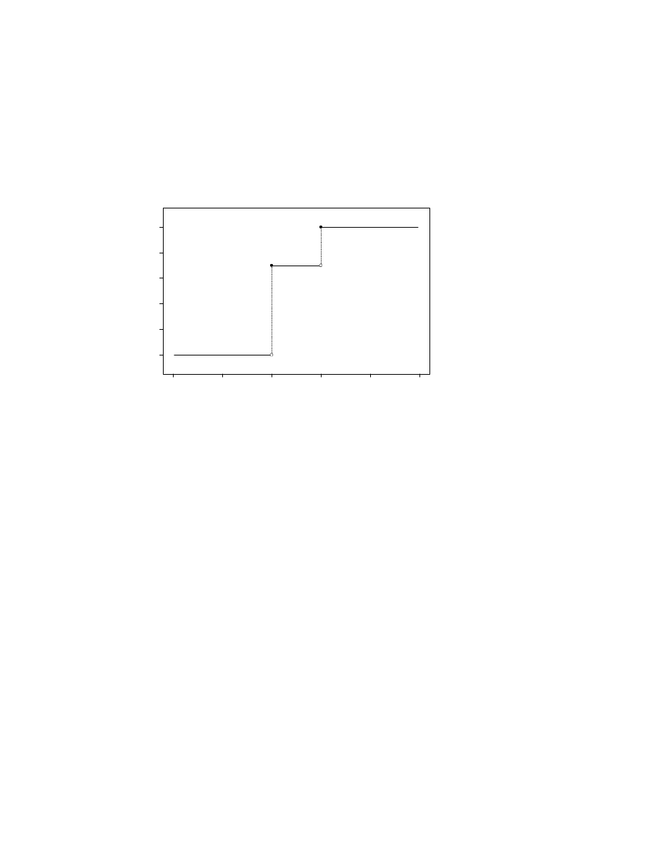
2.5. RANDOM VARIABLES
49
y
F(y)
-2
-1
0
1
2
3
0.0
0.2
0.4
0.6
0.8
1.0
Figure 2.11: Cumulative Distribution Function for Spinning a Typical Penny
• If y < 0, e.g. y = −.5615, then
F (y) = P (X
≤ y) = P (∅) = 0.
• F (0) = P (X ≤ 0) = P ({TT}) = .25.
• If y ∈ (0, 1), e.g. y = .3074, then
F (y) = P (X
≤ y) = P ({TT}) = .25.
• F (1) = P (X ≤ 1) = P ({TT, HT, TH}) = .75.
• If y ∈ (1, 2), e.g. y = 1.4629, then
F (y) = P (X
≤ y) = P ({TT, HT, TH}) = .75.
• F (2) = P (X ≤ 2) = P ({TT, HT, TH, HH}) = 1.
• If y > 2, e.g. y = 2.1252, then
F (y) = P (X
≤ y) = P ({TT, HT, TH, HH}) = 1.
The entire cdf is plotted in Figure 2.12.
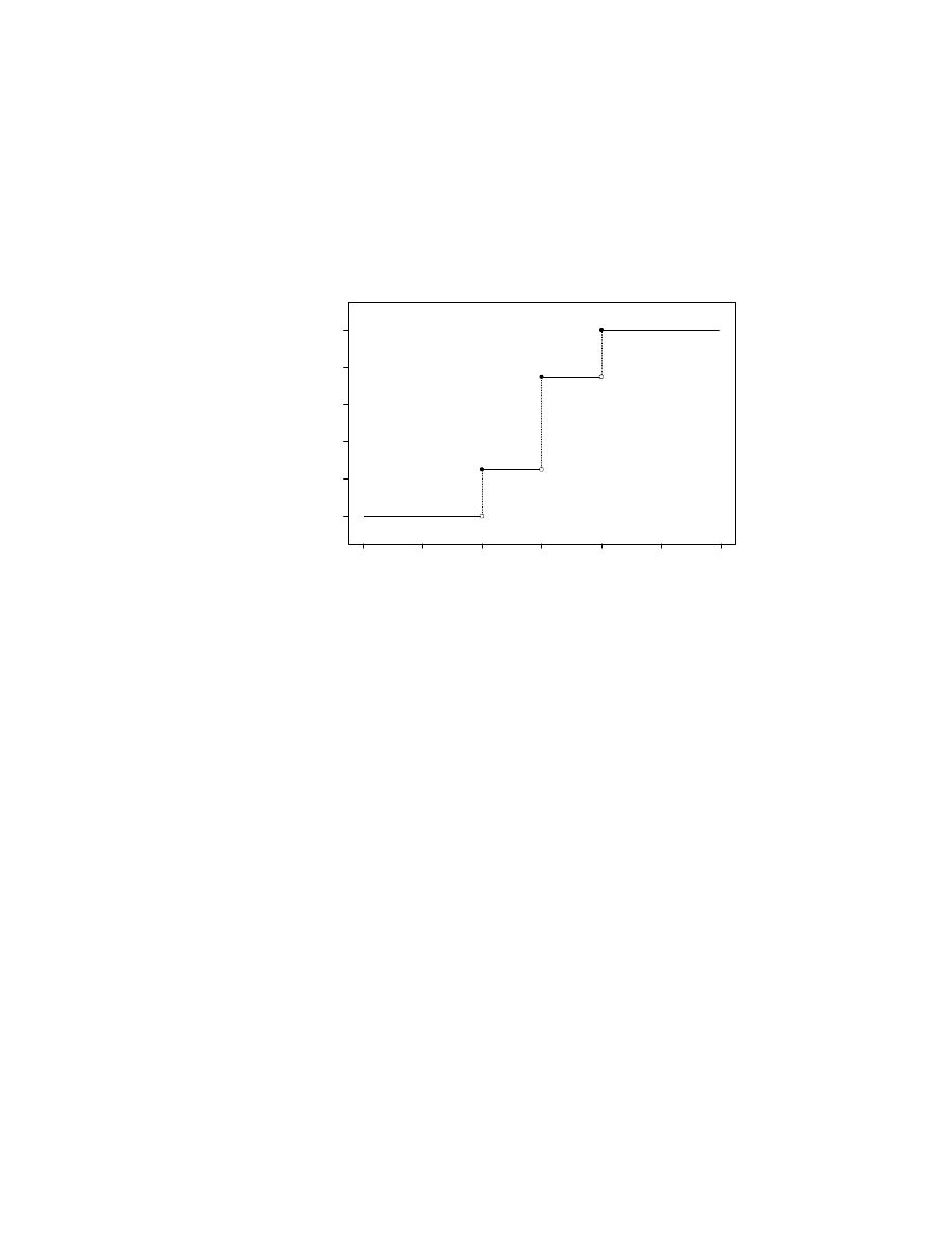
50
CHAPTER 2. PROBABILITY
y
F(y)
-2
-1
0
1
2
3
4
0.0
0.2
0.4
0.6
0.8
1.0
Figure 2.12: Cumulative Distribution Function for Tossing Two Typical
Pennies
Let us make some observations about the cdfs that we have plotted.
First, each cdf assumes its values in the unit interval, [0, 1]. This is a general
property of cdfs: each F (y) = P (X
≤ y), and probabilities necessarily
assume values in [0, 1].
Second, each cdf is nondecreasing; i.e., if y
2
> y
1
, then F (y
2
)
≥ F (y
1
).
This is also a general property of cdfs, for suppose that we observe an out-
come s such that X(s)
≤ y
1
. Because y
1
< y
2
, it follows that X(s)
≤ y
2
.
Thus,
{X ≤ y
1
} ⊂ {X ≤ y
2
} and therefore
F (y
1
) = P (X
≤ y
1
)
≤ P (X ≤ y
2
) = F (y
2
) .
Finally, each cdf equals 1 for sufficiently large y and 0 for sufficiently
small y. This is not a general property of cdfs—it occurs in our examples
because X(S) is a bounded set, i.e. there exist finite real numbers a and b
such that every x
∈ X(S) satisfies a ≤ x ≤ b. However, all cdfs do satisfy
the following properties:
lim
y→∞
F (y) = 1 and
lim
y→−∞
F (y) = 0.

2.6. EXERCISES
51
Independence
We say that two random variables, X
1
and X
2
, are inde-
pendent if each event defined by X
1
is independent of each event defined by
X
2
. More precisely,
Definition 2.6 Let X
1
: S
→ < and X
2
: S
→ < be random variables. X
1
and X
2
are independent if and only if, for each y
1
∈ < and each y
2
∈ <,
P (X
1
≤ y
1
, X
2
≤ y
2
) = P (X
1
≤ y
1
)
· P (X
2
≤ y
2
).
This definition can be extended to mutually independent collections of ran-
dom variables in precisely the same way that we extended Definition 2.2 to
Definition 2.3.
Intuitively, two random variables are independent if the distribution of
either does not depend on the value of the other. As we discussed in Section
2.4, in most applications we will appeal to common sense, our knowledge of
science, etc., to decide if independence is a property that we wish to incorpo-
rate into our mathematical model of the experiment in question. If it is, then
we will assume that the appropriate random variables are independent. This
assumption will allow us to apply many powerful theorems from probability
and statistics that are only true of independent random variables.
2.6
Exercises
1. Consider three events that might occur when a new mine is dug in the
Cleveland National Forest in San Diego County, California:
A
=
{ quartz specimens are found }
B
=
{ tourmaline specimens are found }
C
=
{ aquamarine specimens are found }
Assume the following probabilities: P (A) = .80, P (B) = .36, P (C) =
.28, P (A
∩ B) = .29, P (A ∩ C) = .24, P (B ∩ C) = .16, and P (A ∩ B ∩
C) = .13.
(a) Draw a suitable Venn diagram for this situation.
(b) Calculate the probability that both quartz and tourmaline will be
found, but not aquamarine.
(c) Calculate the probability that quartz will be found, but not tour-
maline or aquamarine.

52
CHAPTER 2. PROBABILITY
(d) Calculate the probability that none of these types of specimens
will be found.
(e) Calculate the probability of A
c
∩ (B ∪ C).
2. Suppose that four fair dice are tossed simultaneously.
(a) How many outcomes are possible?
(b) What is the probability that each top face shows a different num-
ber?
(c) What is the probability that the top faces show four numbers that
sum to five?
(d) What is the probability that at least one of the top faces shows
an odd number?
(e) What is the probability that three of the top faces show the same
odd number and the other top face shows an even number?
3. Consider a standard deck of playing cards and assume that two players
are each dealt five cards. Your answers to the following questions
should be given in the form of suitable arithmetic expressions—it is
not necessary to simplify an answer to a single number.
(a) How many ways are there of dealing the two hands?
(b) What is the probability that the first player will be dealt five
black cards and the second player will be dealt five red cards?
(c) What is the probability that neither player will be dealt an ace?
(d) What is the probability that at least one player will be dealt
exactly two aces?
(e) What is the probability that the second card dealt to the second
player is the ace of spades?
4. Suppose that P (A) = .7, P (B) = .6, and P (A
c
∩ B) = .2.
(a) Draw a Venn diagram that describes this experiment.
(b) Is it possible for A and B to be disjoint events? Why or why not?
(c) What is the probability of A
∪ B
c
?
(d) Is it possible for A and B to be independent events? Why or why
not?

2.6. EXERCISES
53
(e) What is the conditional probability of A given B?
5. Mike owns a box that contains 6 pairs of 14-carat gold, cubic zirconia
earrings. The earrings are of three sizes: 3mm, 4mm, and 5mm. There
are 2 pairs of each size.
Each time that Mike needs an inexpensive gift for a female friend, he
randomly selects a pair of earrings from the box. If the selected pair is
4mm, then he buys an identical pair to replace it. If the selected pair
is 3mm, then he does not replace it. If the selected pair is 5mm, then
he tosses a fair coin. If he observes Heads, then he buys two identical
pairs of earrings to replace the selected pair; if he observes Tails, then
he does not replace the selected pair.
(a) What is the probability that the second pair selected will be 4mm?
(b) If the second pair was not 4mm, then what is the probability that
the first pair was 5mm?
6. The following puzzle was presented on National Public Radio’s Car
Talk:
RAY: Three different numbers are chosen at random, and
one is written on each of three slips of paper. The slips are
then placed face down on the table. The objective is to
choose the slip upon which is written the largest number.
Here are the rules: You can turn over any slip of paper
and look at the amount written on it. If for any reason you
think this is the largest, you’re done; you keep it. Otherwise
you discard it and turn over a second slip. Again, if you
think this is the one with the biggest number, you keep that
one and the game is over. If you don’t, you discard that one
too.
TOM: And you’re stuck with the third. I get it.
RAY: The chance of getting the highest number is one in
three. Or is it? Is there a strategy by which you can improve
the odds?
7. For each of the following pairs of events, explain why A and B are
dependent or independent.

54
CHAPTER 2. PROBABILITY
(a) Consider the population of U.S. citizens, from which a person is
randomly selected. Let A denote the event that the person is a
member of a chess club and let B denote the event that the person
is a woman.
(b) Consider the population of male U.S. citizens who are 30 years of
age. A man is selected at random from this population. Let A
denote the event that he will be bald before reaching 40 years of
age and let B denote the event that his father went bald before
reaching 40 years of age.
(c) Consider the population of students who attend high school in
the U.S. A student is selected at random from this population.
Let A denote the event that the student speaks Spanish and let
B denote the event that the student lives in Texas.
(d) Consider the population of months in the 20th century. A month
is selected at random from this population. Let A denote the
event that a hurricane crossed the North Carolina coastline during
this month and let B denote the event that it snowed in Denver,
Colorado, during this month.
(e) Consider the population of Hollywood feature films produced dur-
ing the 20th century. A movie is selected at random from this
population. Let A denote the event that the movie was filmed in
color and let B denote the event that the movie is a western.
8. Suppose that X is a random variable with cdf
F (y) =
0
y
≤ 0
y/3
y
∈ [0, 1)
2/3
y
∈ [1, 2]
y/3
y
∈ [2, 3]
1
y
≥ 3
.
Graph F and compute the following probabilities:
(a) P (X > .5)
(b) P (2 < X
≤ 3)
(c) P (.5 < X
≤ 2.5)
(d) P (X = 1)

Chapter 3
Discrete Random Variables
3.1
Basic Concepts
Our introduction of random variables in Section 2.5 was completely general,
i.e. the principles that we discussed apply to all random variables. In this
chapter, we will study an important special class of random variables, the
discrete random variables. One of the advantages of restricting attention to
discrete random variables is that the mathematics required to define various
fundamental concepts for this class is fairly minimal.
We begin with a formal definition.
Definition 3.1 A random variable X is discrete if X(S), the set of possible
values of X, is countable.
Our primary interest will be in random variables for which X(S) is finite;
however, there are many important random variables for which X(S) is denu-
merable. The methods described in this chapter apply to both possibilities.
In contrast to the cumulative distribution function (cdf) defined in Sec-
tion 2.5, we now introduce the probability mass function (pmf).
Definition 3.2 Let X be a discrete random variable. The probability mass
function (pmf ) of X is the function f :
< → < defined by
f (x) = P (X = x).
If f is the pmf of X, then f necessarily possesses several properties worth
noting:
1. f (x)
≥ 0 for every x ∈ <.
55

56
CHAPTER 3. DISCRETE RANDOM VARIABLES
2. If x
6∈ X(S), then f(x) = 0.
3. By the definition of X(S),
X
x∈X(S)
f (x) =
X
x∈X(S)
P (X = x) = P
[
x∈X(S)
{x}
= P (X
∈ X(S))
= 1.
There is an important relation between the pmf and the cdf. For each
y
∈ <, let
L(y) =
{x ∈ X(S) : x ≤ y}
denote the values of X that are less than or equal to y. Then
F (y) = P (X
≤ y) = P (X ∈ L(y))
=
X
x∈L(y)
P (X = x)
=
X
x∈L(y)
f (x).
(3.1)
Thus, the value of the cdf at y can be obtained by summing the values of
the pmf at all values x
≤ y.
More generally, we can compute the probability that X assumes its value
in any set B
⊂ < by summing the values of the pmf over all values of X
that lie in B. Here is the formula:
P (X
∈ B) =
X
x∈X(S)∩B
P (X = x) =
X
x∈X(S)∩B
f (x).
(3.2)
We now turn to some elementary examples of discrete random variables
and their pmfs.
3.2
Examples
Example 1
A fair coin is tossed and the outcome is Heads or Tails.
Define a random variable X by X(Heads) = 1 and X(Tails) = 0.
The pmf of X is the function f defined by
f (0) = P (X = 0) = .5,
f (1) = P (X = 1) = .5,
and f (x) = 0 for all x
6∈ X(S) = {0, 1}.

3.2. EXAMPLES
57
Example 2
A typical penny is spun and the outcome is Heads or
Tails
. Define a random variable X by X(Heads) = 1 and X(Tails) = 0.
The pmf of X is (approximately) the function f defined by
f (0) = P (X = 0) = .7,
f (1) = P (X = 1) = .3,
and f (x) = 0 for all x
6∈ X(S) = {0, 1}.
Example 3
A fair die is tossed and the number of dots on the upper
face is observed. The sample space is S =
{1, 2, 3, 4, 5, 6}. Define a random
variable X by X(s) = 1 if s is a prime number and X(s) = 0 if s is not a
prime number.
The pmf of X is the function f defined by
f (0) = P (X = 0) = P (
{4, 6}) = 1/3,
f (1) = P (X = 1) = P (
{1, 2, 3, 5}) = 2/3,
and f (x) = 0 for all x
6∈ X(S) = {0, 1}.
Examples 1–3 have a common structure that we proceed to generalize.
Definition 3.3 A random variable X is a Bernoulli trial if X(S) =
{0, 1}.
Traditionally, we call X = 1 a “success” and X = 0 a “failure”.
The family of probability distributions of Bernoulli trials is parametrized
(indexed) by a real number p
∈ [0, 1], usually by setting p = P (X = 1).
We communicate that X is a Bernoulli trial with success probability p by
writing X
∼ Bernoulli(p). The pmf of such a random variable is the function
f defined by
f (0) = P (X = 0) = 1
− p,
f (1) = P (X = 1) = p,
and f (x) = 0 for all x
6∈ X(S) = {0, 1}.
Several important families of random variables can be derived from Ber-
noulli trials. Consider, for example, the familiar experiment of tossing a
fair coin twice and counting the number of Heads. In Section 3.4, we will
generalize this experiment and count the number of successes in n Bernoulli
trials. This will lead to the family of binomial probability distributions.

58
CHAPTER 3. DISCRETE RANDOM VARIABLES
Bernoulli trials are also a fundamental ingredient of the St. Petersburg
Paradox, described in Example 7 of Section 3.3. In this experiment, a
fair coin is tossed until Heads was observed and the number of Tails was
counted. More generally, consider an experiment in which a sequence of
independent Bernoulli trials, each with success probability p, is performed
until the first success is observed. Let X
1
, X
2
, X
3
, . . . denote the individual
Bernoulli trials and let Y denote the number of failures that precede the first
success. Then the possible values of Y are Y (S) =
{0, 1, 2, . . .} and the pmf
of Y is
f (j) = P (Y = j) = P (X
1
= 0, . . . , X
j
= 0, X
j+1
= 1)
= P (X
1
= 0)
· · · P (X
j
= 0)
· P (X
j+1
= 1)
= (1
− p)
j
p
if j
∈ Y (S) and f(j) = 0 if j 6∈ Y (S). This family of probability distributions
is also parametrized by a real number p
∈ [0, 1]. It is called the geometric
family and a random variable with a geometric distribution is said to be a
geometric random variable, written Y
∼ Geometric(p).
If Y
∼ Geometric(p) and k ∈ Y (S), then
F (k) = P (Y
≤ k) = 1 − P (Y > k) = 1 − P (Y ≥ k + 1).
Because the event
{Y ≥ k + 1} occurs if and only if X
1
=
· · · X
k+1
= 0, we
conclude that
F (k) = 1
− (1 − p)
k+1
.
Example 4
Gary is a college student who is determined to have a date
for an approaching formal. He believes that each woman he asks is twice
as likely to decline his invitation as to accept it, but he resolves to extend
invitations until one is accepted. However, each of his first ten invitations is
declined. Assuming that Gary’s assumptions about his own desirability are
correct, what is the probability that he would encounter such a run of bad
luck?
Gary evidently believes that he can model his invitations as a sequence
of independent Bernoulli trials, each with success probability p = 1/3. If
so, then the number of unsuccessful invitations that he extends is a random
variable Y
∼ Geometric(1/3) and
P (Y
≥ 10) = 1 − P (Y ≤ 9) = 1 − F (9) = 1 −
"
1
−
µ
2
3
10
#
.
= .0173.

3.2. EXAMPLES
59
Either Gary is very unlucky or his assumptions are flawed. Perhaps
his probability model is correct, but p < 1/3. Perhaps, as seems likely,
the probability of success depends on who he asks. Or perhaps the trials
were not really independent.
1
If Gary’s invitations cannot be modelled as
independent and identically distributed Bernoulli trials, then the geometric
distribution cannot be used.
Another important family of random variables is often derived by con-
sidering an urn model. Imagine an urn that contains m red balls and n black
balls. The experiment of present interest involves selecting k balls from the
urn in such a way that each of the
¡
m+n
k
¢
possible outcomes that might be
obtained are equally likely. Let X denote the number of red balls selected
in this manner. If we observe X = x, then x red balls were selected from
a total of m red balls and k
− x black balls were selected from a total of n
black balls. Evidently, x
∈ X(S) if and only if x is an integer that satisfies
x
≤ min(m, k) and k − x ≤ min(n, k). Furthermore, if x ∈ X(S), then the
pmf of X is
f (x) = P (X = x) =
#
{X = x}
#S
=
¡
m
x
¢¡
n
k−x
¢
¡
m+n
k
¢
.
This family of probability distributions is parametrized by a triple of integers,
(m, n, k), for which m, n
≥ 0, m + n ≥ 1, and 0 ≤ k ≤ m + n. It is called
the hypergeometric family and a random variable with a hypergeometric
distribution is said to be a hypergeometric random variable, written Y
∼
Hypergeometric(m, n, k).
The trick to using the hypergeometric distribution in applications is to
recognize a correspondence between the actual experiment and an idealized
urn model, as in. . .
Example 5
(Adapted from an example analyzed by R.R. Sokal and
F.J. Rohlf (1969), Biometry: The Principles and Practice of Statistics in
Biological Research, W.H. Freeman and Company, San Francisco.)
All but 28 acacia trees (of the same species) were cleared from a study
area in Central America. The 28 remaining trees were freed from ants by one
of two types of insecticide. The standard insecticide (A) was administered
1
In the actual incident on which this example is based, the women all lived in the same
residential college
. It seems doubtful that each woman was completely unaware of the
invitation that preceded hers.

60
CHAPTER 3. DISCRETE RANDOM VARIABLES
to 15 trees; an experimental insecticide (B) was administered to the other 13
trees. The assignment of insectides to trees was completely random. At issue
was whether or not the experimental insecticide was more effective than the
standard insecticide in inhibiting future ant infestations.
Next, 16 separate ant colonies were situated roughly equidistant from the
acacia trees and permitted to invade them. Unless food is scarce, different
colonies will not compete for the same resources; hence, it could be presumed
that each colony would invade a different tree. In fact, the ants invaded 13
of the 15 trees treated with the standard insecticide and only 3 of the 13
trees treated with the experimental insecticide. If the two insecticides were
equally effective in inhibiting future infestations, then what is the probability
that no more than 3 ant colonies would have invaded trees treated with the
experimental insecticide?
This is a potentially confusing problem that is simplified by construct-
ing an urn model for the experiment. There are m = 13 trees with the
experimental insecticide (red balls) and n = 15 trees with the standard
insecticide (black balls). The ants choose k = 16 trees (balls). Let X de-
note the number of experimental trees (red balls) invaded by the ants; then
X
∼ Hypergeometric(13, 15, 16) and its pmf is
f (x) = P (X = x) =
¡
13
x
¢¡
15
16−x
¢
¡
28
16
¢
.
Notice that there are not enough standard trees for each ant colony to invade
one; hence, at least one ant colony must invade an experimental tree and
X = 0 is impossible. Thus,
P (X
≤ 3) = f(1) + f(2) + f(3) =
¡
13
1
¢¡
15
15
¢
¡
28
16
¢
+
¡
13
2
¢¡
15
14
¢
¡
28
16
¢
+
¡
13
3
¢¡
15
13
¢
¡
28
16
¢
.
= .0010.
This reasoning illustrates the use of a statistical procedure called Fisher’s
exact test. The probability that we have calculated is an example of what
we will later call a significance probability. In the present example, the fact
that the significance probability is so small would lead us to challenge an
assertion that the experimental insecticide is no better than the standard
insecticide.
It is evident that calculations with the hypergeometric distribution can
become rather tedious. Accordingly, this is a convenient moment to intro-
duce computer software for the purpose of evaluating certain pmfs and cdfs.

3.3. EXPECTATION
61
The statistical programming language S-Plus includes functions that evalu-
ate pmfs and cdfs for a variety of distributions, including the geometric and
hypergeometric. For the geometric, these functions are dgeom and pgeom;
for the hypergeometric, these functions are dhyper and phyper. We can
calculate the probability in Example 4 as follows:
> 1-pgeom(q=9,prob=1/3)
[1] 0.01734153
Similarly, we can calculate the probability in Example 5 as follows:
> phyper(q=3,m=13,n=15,k=16)
[1] 0.001026009
3.3
Expectation
Sometime in the early 1650s, the eminent theologian and amateur mathe-
matician Blaise Pascal found himself in the company of the Chevalier de
M´er´e.
2
De M´er´e posed to Pascal a famous problem: how to divide the pot
of an interrupted dice game. Pascal communicated the problem to Pierre
de Fermat in 1654, beginning a celebrated correspondence that established
a foundation for the mathematics of probability.
Pascal and Fermat began by agreeing that the pot should be divided
according to each player’s chances of winning it. For example, suppose that
each of two players has selected a number from the set S =
{1, 2, 3, 4, 5, 6}.
For each roll of a fair die that produces one of their respective numbers, the
corresponding player receives a token. The first player to accumulate five
tokens wins a pot of $100. Suppose that the game is interrupted with Player
A having accumulated four tokens and Player B having accumulated only
one. The probability that Player B would have won the pot had the game
been completed is the probability that B’s number would have appeared
four more times before A’s number appeared one more time. Because we can
ignore rolls that produce neither number, this is equivalent to the probability
that a fair coin will have a run of four consecutive Heads, i.e. .5
· .5 · .5 ·
.5 = .0625. Hence, according to Pascal and Fermat, Player B is entitled to
.0625
· $100 = $6.25 from the pot and Player A is entitled to the remaining
$93.75.
2
This account of the origins of modern probability can be found in Chapter 6 of David
Bergamini’s Mathematics, Life Science Library, Time Inc., New York, 1963.

62
CHAPTER 3. DISCRETE RANDOM VARIABLES
The crucial concept in Pascal’s and Fermat’s analysis is the notion that
each prospect should be weighted by the chance of realizing that prospect.
This notion motivates
Definition 3.4 The expected value of a discrete random variable X, which
we will denote E(X) or simply EX, is the probability-weighted average of the
possible values of X, i.e.
EX =
X
x∈X(S)
xP (X = x) =
X
x∈X(S)
xf (x).
Remark
The expected value of X, EX, is often called the population
mean and denoted µ.
Example 1
If X
∼ Bernoulli(p), then
µ = EX =
X
x∈{0,1}
xP (X = x) = 0
·P (X = 0)+1·P (X = 1) = P (X = 1) = p.
Fair Value
The expected payoff of a game of chance is sometimes called
the fair value of the game. For example, suppose that you own a slot ma-
chine that pays a jackpot of $1000 with probability p = .0005 and $0 with
probability 1
− p = .9995. How much should you charge a customer to play
this machine? Letting X denote the payoff (in dollars), the expected payoff
per play is
EX = 1000
· .0005 + 0 · .9995 = .5;
hence, if you want to make a profit, then you should charge more than $0.50
per play. Suppose, however, that a rival owner of an identical slot machine
attempted to compete for the same customers. According to the theory of
microeconomics, competition would cause each of you to try to undercut the
other, eventually resulting in an equilibrium price of exactly $0.50 per play,
the fair value of the game.
We proceed to illustrate both the mathematics and the psychology of fair
value by considering several lotteries. A lottery is a choice between receiving
a certain payoff and playing a game of chance. In each of the following
examples, we emphasize that the value accorded the game of chance by a
rational person may be very different from the game’s expected value. In
this sense, the phrase “fair value” is often a misnomer.

3.3. EXPECTATION
63
Example 2a
You are offered the choice between receiving a certain $5
and playing the following game: a fair coin is tossed and you receive $10 or
$0 according to whether Heads or Tails is observed.
The expected payoff from the game (in dollars) is
EX = 10
· .5 + 0 · .5 = 5,
so your options are equivalent with respect to expected earnings. One might
therefore suppose that a rational person would be indifferent to which option
he or she selects. Indeed, in my experience, some students prefer to take the
certain $5 and some students prefer to gamble on perhaps winning $10. For
this example, the phrase “fair value” seems apt.
Example 2b
You are offered the choice between receiving a certain
$5000 and playing the following game: a fair coin is tossed and you receive
$10,000 or $0 according to whether Heads or Tails is observed.
The mathematical structure of this lottery is identical to that of the
preceding lottery, except that the stakes are higher. Again, the options are
equivalent with respect to expected earnings; again, one might suppose that
a rational person would be indifferent to which option he or she selects.
However, many students who opt to gamble on perhaps winning $10 in
Example 2a opt to take the certain $5000 in Example 2b.
Example 2c
You are offered the choice between receiving a certain $1
million and playing the following game: a fair coin is tossed and you receive
$2 million or $0 according to whether Heads or Tails is observed.
The mathematical structure of this lottery is identical to that of the
preceding two lotteries, except that the stakes are now much higher. Again,
the options are equivalent with respect to expected earnings; however, almost
every student to whom I have presented this lottery has expressed a strong
preference for taking the certain $1 million.
Example 3
You are offered the choice between receiving a certain $1
million and playing the following game: a fair coin is tossed and you receive
$5 million or $0 according to whether Heads or Tails is observed.
The expected payoff from this game (in millions of dollars) is
EX = 5
· .5 + 0 · .5 = 2.5,

64
CHAPTER 3. DISCRETE RANDOM VARIABLES
so playing the game is the more attractive option with respect to expected
earnings. Nevertheless, most students opt to take the certain $1 million. This
should not be construed as an irrational decision. For example, the addition
of $1 million to my own modest estate would secure my eventual retirement.
The addition of an extra $4 million would be very pleasant indeed, allowing
me to increase my current standard of living. However, I do not value the
additional $4 million nearly as much as I value the initial $1 million. As
Aesop observed, “A little thing in hand is worth more than a great thing in
prospect.” For this example, the phrase “fair value” introduces normative
connotations that are not appropriate.
Example 4
Consider the following passage from a recent article about
investing:
“. . . it’s human nature to overweight low probabilities that offer
high returns. In one study, subjects were given a choice between
a 1-in-1000 chance to win $5000 or a sure thing to win $5; or a 1-
in-1000 chance of losing $5000 versus a sure loss of $5. In the first
case, the expected value (mathematically speaking) is making $5.
In the second case, it’s losing $5. Yet in the first situation, which
mimics a lottery, more than 70% of people asked chose to go for
the $5000. In the second situation, more than 80% would take
the $5 hit.”
3
The author evidently considered the reported preferences paradoxical, but
are they really surprising? Plus or minus $5 will not appreciably alter the
financial situations of most subjects, but plus or minus $5000 will. It is
perfectly rational to risk a negligible amount on the chance of winning $5000
while declining to risk a negligible amount on the chance of losing $5000.
The following examples further explicate this point.
Example 5
The same article advises, “To limit completely irrational
risks, such as lottery tickets, try speculating only with money you would
otherwise use for simple pleasures, such as your morning coffee.”
Consider a hypothetical state lottery, in which 5 numbers are drawn
(without replacement) from the set
{1, 2, . . . , 39, 40}. For $2, you can pur-
chase a ticket that specifies 6 such numbers. If the numbers on your ticket
3
Robert Frick, “The 7 Deadly Sins of Investing,” Kiplinger’s Personal Finance Maga-
zine
, March 1998, p. 138.

3.3. EXPECTATION
65
match the numbers selected by the state, then you win $1 million; otherwise,
you win nothing. (For the sake of simplicity, we ignore the possibility that
you might have to split the jackpot with other winners and the possibility
that you might win a lesser prize.) Is buying a lottery ticket “completely
irrational”?
The probability of winning the lottery in question is
p =
1
¡
40
6
¢
=
1
3, 838, 380
.
= 2.6053
× 10
−7
,
so your expected prize (in dollars) is approximately
10
6
· 2.6053 × 10
−7
.
= 0.26,
which is considerably less than the cost of a ticket. Evidently, it is completely
irrational to buy tickets for this lottery as an investment strategy. Suppose,
however, that I buy one ticket per week and reason as follows: I will almost
certainly lose $2 per week, but that loss will have virtually no impact on my
standard of living; however, if by some miracle I win, then gaining $1 million
will revolutionize my standard of living. This can hardly be construed as
irrational behavior, although Robert Frick’s advice to speculate only with
funds earmarked for entertainment is well-taken.
In most state lotteries, the fair value of the game is less than the cost of
a lottery ticket. This is only natural—lotteries exist because they generate
revenue for the state that runs them! (By the same reasoning, gambling must
favor the house because casinos make money for their owners.) However, on
very rare occasions a jackpot is so large that the typical situation is reversed.
Several years ago, an Australian syndicate noticed that the fair value of a
Florida state lottery exceeded the price of a ticket and purchased a large
number of tickets as an (ultimately successful) investment strategy. And
Voltaire once purchased every ticket in a raffle upon noting that the prize
was worth more than the total cost of the tickets being sold!
Example 6
If the first case described in Example 4 mimics a lottery,
then the second case mimics insurance. Mindful that insurance companies
(like casinos) make money, Ambrose Bierce offered the following definition:
“INSURANCE, n. An ingenious modern game of chance in which
the player is permitted to enjoy the comfortable conviction that

66
CHAPTER 3. DISCRETE RANDOM VARIABLES
he is beating the man who keeps the table.”
4
However, while it is certainly true that the fair value of an insurance policy
is less than the premiums required to purchase it, it does not follow that
buying insurance is irrational. I can easily afford to pay $200 per year for
homeowners insurance, but I would be ruined if all of my possessions were
destroyed by fire and I received no compensation for them. My decision that
a certain but affordable loss is preferable to an unlikely but catastrophic loss
is an example of risk-averse behavior.
Before presenting our concluding example of fair value, we derive a useful
formula. Suppose that X : S
→ < is a discrete random variable and φ : < →
< is a function. Let Y = φ(X). Then Y is a random variable and
Eφ(X) = EY =
X
y∈Y (S)
yP (Y = y)
=
X
y∈Y (S)
yP (φ(X) = y)
=
X
y∈Y (S)
yP
³
X
∈ φ
−1
(y)
´
=
X
y∈Y (S)
y
X
x∈φ
−
1
(y)
P (X = x)
=
X
y∈Y (S)
X
x∈φ
−
1
(y)
yP (X = x)
=
X
y∈Y (S)
X
x∈φ
−
1
(y)
φ(x)P (X = x)
=
X
x∈X(S)
φ(x)P (X = x)
=
X
x∈X(S)
φ(x)f (x).
(3.3)
Example 7
Consider a game in which the jackpot starts at $1 and
doubles each time that Tails is observed when a fair coin is tossed. The
game terminates when Heads is observed for the first time. How much would
4
Ambrose Bierce, The Devil’s Dictionary, 1881–1906. In The Collected Writings of
Ambrose Bierce
, Citadel Press, Secaucus, NJ, 1946.

3.3. EXPECTATION
67
you pay for the privilege of playing this game? How much would you charge
if you were responsible for making the payoff ?
This is a curious game. With high probability, the payoff will be rather
small; however, there is a small chance of a very large payoff. In response to
the first question, most students discount the latter possibility and respond
that they would only pay a small amount, rarely more than $4. In response to
the second question, most students recognize the possibility of a large payoff
and demand payment of a considerably greater amount. Let us consider if
the notion of fair value provides guidance in reconciling these perspectives.
Let X denote the number of Tails that are observed before the game
terminates. Then X(S) =
{0, 1, 2, . . .} and the geometric random variable
X has pmf
f (x) = P (x consecutive Tails) = .5
x
.
The payoff from this game (in dollars) is Y = 2
X
; hence, the expected
payoff is
E2
X
=
∞
X
x=0
2
x
· .5
x
=
∞
X
x=0
1 =
∞.
This is quite startling! The “fair value” of this game provides very little
insight into the value that a rational person would place on playing it. This
remarkable example is quite famous—it is known as the St. Petersburg Para-
dox.
Properties of Expectation
We now state (and sometimes prove) some
useful consequences of Definition 3.4 and Equation 3.3.
Theorem 3.1 Let X denote a discrete random variable and suppose that
P (X = c) = 1. Then EX = c.
Theorem 3.1 states that, if a random variable always assumes the same
value c, then the probability-weighted average of the values that it assumes
is c. This should be obvious.
Theorem 3.2 Let X denote a discrete random variable and suppose that
c
∈ < is constant. Then
E [cφ(X)] =
X
x∈X(S)
cφ(x)f (x) = c
X
x∈X(S)
φ(x)f (x) = cE [φ(X)] .

68
CHAPTER 3. DISCRETE RANDOM VARIABLES
Theorem 3.2 states that we can interchange the order of multiplying by
a constant and computing the expected value. Notice that this property of
expectation follows directly from the analogous property for summation.
Theorem 3.3 Let X denote a discrete random variable. Then
E [φ
1
(X) + φ
2
(X)] =
X
x∈X(S)
[φ
1
(x) + φ
2
(x)]f (x)
=
X
x∈X(S)
[φ
1
(x)f (x) + φ
2
(x)f (x)]
=
X
x∈X(S)
φ
1
(x)f (x) +
X
x∈X(S)
φ
2
(x)f (x)
= E [φ
1
(X)] + E [φ
2
(X)] .
Theorem 3.3 states that we can interchange the order of adding functions
of a random variable and computing the expected value. Again, this property
of expectation follows directly from the analogous property for summation.
Theorem 3.4 Let X
1
and X
2
denote discrete random variables. Then
E [X
1
+ X
2
] = EX
1
+ EX
2
.
Theorem 3.4 states that the expected value of a sum equals the sum of
the expected values.
Variance
Now suppose that X is a discrete random variable, let µ = EX
denote its expected value, or population mean., and define a function φ :
< → < by
φ(x) = (x
− µ)
2
.
For any x
∈ <, φ(x) is the squared deviation of x from the expected value
of X. If X always assumes the value µ, then φ(X) always assumes the value
0; if X tends to assume values near µ, then φ(X) will tend to assume small
values; if X often assumes values far from µ, then φ(X) will often assume
large values. Thus, Eφ(X), the expected squared deviation of X from its
expected value, is a measure of the variability of the population X(S). We
summarize this observation in

3.3. EXPECTATION
69
Definition 3.5 The variance of a discrete random variable X, which we
will denote Var(X) or simply Var X, is the probability-weighted average of
the squared deviations of X from EX = µ, i.e.
Var X = E(X
− µ)
2
=
X
x∈X(S)
(x
− µ)
2
f (x).
Remark
The variance of X, Var X, is often called the population vari-
ance and denoted σ
2
.
Denoting the population variance by σ
2
may strike the reader as awk-
ward notation, but there is an excellent reason for it. Because the variance
measures squared deviations from the population mean, it is measured in
different units than either the random variable itself or its expected value.
For example, if X measures length in meters, then so does EX, but Var X is
measured in meters squared. To recover a measure of population variability
in the original units of measurement, we take the square root of the variance
and obtain σ.
Definition 3.6 The standard deviation of a random variable is the square
root of its variance.
Remark
The standard deviation of X, often denoted σ, is often called
the population standard deviation.
Example 1 (continued)
If X
∼ Bernoulli(p), then
σ
2
= Var X = E(X
− µ)
2
= (0
− µ)
2
· P (X = 0) + (1 − µ)
2
· P (X = 1)
= (0
− p)
2
(1
− p) + (1 − p)
2
p
= p(1
− p)(p + 1 − p)
= p(1
− p).
Before turning to a more complicated example, we establish a useful fact.

70
CHAPTER 3. DISCRETE RANDOM VARIABLES
Theorem 3.5 If X is a discrete random variable, then
Var X = E(X
− µ)
2
= E(X
2
− 2µX + µ
2
)
= EX
2
+ E(
−2µX) + Eµ
2
= EX
2
− 2µEX + µ
2
= EX
2
− 2µ
2
+ µ
2
= EX
2
− (EX)
2
.
A straightforward way to calculate the variance of a discrete random variable
that assumes a fairly small number of values is to exploit Theorem 3.5 and
organize one’s calculations in the form of a table.
Example 8
Suppose that X is a random variable whose possible values
are X(S) =
{2, 3, 5, 10}. Suppose that the probability of each of these values
is given by the formula f (x) = P (X = x) = x/20.
(a) Calculate the expected value of X.
(b) Calculate the variance of X.
(c) Calculate the standard deviation of X.
Solution
x f (x) xf (x)
x
2
x
2
f (x)
2
.10
.20
4
.40
3
.15
.45
9
1.35
5
.25
1.25
25
6.25
10
.50
5.00 100
50.0
6.90
58.00
(a) µ = EX = .2 + .45 + 1.25 + 5 = 6.9.
(b) σ
2
= Var X = EX
2
− (EX)
2
= (.4 + 1.35 + 6.25 + 50)
− 6.9
2
=
58
− 47.61 = 10.39.
(c) σ =
√
10.39
.
= 3.2234.

3.3. EXPECTATION
71
Now suppose that X : S
→ < is a discrete random variable and φ : < → <
is a function. Let Y = φ(X). Then Y is a discrete random variable and
Var φ(X) = Var Y = E [Y
− EY ]
2
= E [φ(X)
− Eφ(X)]
2
.
(3.4)
We conclude this section by stating (and sometimes proving) some useful
consequences of Definition 3.5 and Equation 3.4.
Theorem 3.6 Let X denote a discrete random variable and suppose that
c
∈ < is constant. Then
Var(X + c) = Var X.
Although possibly startling at first glance, this result is actually quite
intuitive. The variance depends on the squared deviations of the values of
X from the expected value of X. If we add a constant to each value of X,
then we shift both the individual values of X and the expected value of X
by the same amount, preserving the squared deviations. The variability of
a population is not affected by shifting each of the values in the population
by the same amount.
Theorem 3.7 Let X denote a discrete random variable and suppose that
c
∈ < is constant. Then
Var(cX) = E [cX
− E(cX)]
2
= E [cX
− cEX]
2
= E [c(X
− EX)]
2
= E
h
c
2
(X
− EX)
2
i
= c
2
E(X
− EX)
2
= c
2
Var X.
To understand this result, recall that the variance is measured in the
original units of measurement squared. If we take the square root of each
expression in Theorem 3.7, then we see that one can interchange multiplying
a random variable by a nonnegative constant with computing its standard
deviation.
Theorem 3.8 If the discrete random variables X
1
and X
2
are independent,
then
Var(X
1
+ X
2
) = Var X
1
+ Var X
2
.

72
CHAPTER 3. DISCRETE RANDOM VARIABLES
Theorem 3.8 is analogous to Theorem 3.4. However, in order to ensure
that the variance of a sum equals the sum of the variances, the random
variables must be independent.
3.4
Binomial Distributions
Suppose that a fair coin is tossed twice and the number of Heads is counted.
Let Y denote the total number of Heads. Because the sample space has four
equally likely outcomes, viz.
S =
{HH, HT, TH, TT},
the pmf of Y is easily determined:
f (0) = P (Y = 0) = P (
{HH}) = .25,
f (1) = P (Y = 1) = P (
{HT, TH}) = .5,
f (2) = P (Y = 2) = P (
{TT}) = .25,
and f (y) = 0 if y
6∈ Y (S) = {0, 1, 2}.
Referring to representation (c) of Example 2 in Section 2.5, the above
experiment has the following characteristics:
• Let X
1
denote the number of Heads observed on the first toss and let
X
2
denote the number of Heads observed on the second toss. Then
the random variable of interest is Y = X
1
+ X
2
.
• The random variables X
1
and X
2
are independent.
• The random variables X
1
and X
2
have the same distribution, viz.
X
1
, X
2
∼ Bernoulli(.5).
We proceed to generalize this example in two ways:
1. We allow any finite number of trials.
2. We allow any success probability p
∈ [0, 1].
Definition 3.7 Let X
1
, . . . , X
n
be mutually independent Bernoulli trials,
each with success probability p. Then
Y =
n
X
i=1
X
i

3.4. BINOMIAL DISTRIBUTIONS
73
is a binomial random variable, denoted
Y
∼ Binomial(n; p).
Applying Theorem 3.4, we see that the expected value of a binomial
random variable is the product of the number of trials and the probability
of success:
EY = E
Ã
n
X
i=1
X
i
!
=
n
X
i=1
EX
i
=
n
X
i=1
p = np.
Furthermore, because the trials are independent, we can apply Theorem 3.8
to calculate the variance:
Var Y = Var
Ã
n
X
i=1
X
i
!
=
Ã
n
X
i=1
Var X
i
!
=
Ã
n
X
i=1
p(1
− p)
!
= np(1
− p).
Because Y counts the total number of successes in n Bernoulli trials, it
should be apparent that Y (S) =
{0, 1, . . . , n}. Let f denote the pmf of Y .
For fixed n, p, and j
∈ Y (S), we wish to determine
f (j) = P (Y = j).
To illustrate the reasoning required to make this determination, suppose
that there are n = 6 trials, each with success probability p = .3, and that we
wish to determine the probability of observing exactly j = 2 successes. Some
examples of experimental outcomes for which Y = 2 include the following:
110000 000011 010010
Because the trials are mutually independent, we see that
P (110000) = .3
· .3 · .7 · .7 · .7 · .7 = .3
2
· .7
4
,
P (000011) = .7
· .7 · .7 · .7 · .3 · .3 = .3
2
· .7
4
,
P (010010) = .7
· .3 · .7 · .7 · .3 · .7 = .3
2
· .7
4
.
It should be apparent that the probability of each outcome for which Y = 2
is the product of j = 2 factors of p = .3 and n
− j = 4 factors of 1 − p = .7.
Furthermore, the number of such outcomes is the number of ways of choosing
j = 2 successes from a total of n = 6 trials. Thus,
f (2) = P (Y = 2) =
Ã
6
2
!
.3
2
.7
4

74
CHAPTER 3. DISCRETE RANDOM VARIABLES
for the specific example in question and the general formula for the binomial
pmf is
f (j) = P (Y = j) =
Ã
n
j
!
p
j
(1
− p)
n−j
.
It follows, of course, that the general formula for the binomial cdf is
F (k) = P (Y
≤ k) =
k
X
j=0
P (Y = j) =
k
X
j=0
f (j)
=
k
X
j=0
Ã
n
j
!
p
j
(1
− p)
n−j
.
(3.5)
Except for very small numbers of trials, direct calculation of (3.5) is
rather tedious. Fortunately, tables of the binomial cdf for selected values of
n and p are widely available, as is computer software for evaluating (3.5).
In the examples that follow, we will evaluate (3.5) using the S-Plus function
pbinom
.
As the following examples should make clear, the trick to evaluating bi-
nomial probabilities is to write them in expressions that only involve prob-
abilities of the form P (Y
≤ k).
Example 1
In 10 trials with success probability .5, what is the proba-
bility that no more than 4 successes will be observed?
Here, n = 10, p = .5, and we want to calculate
P (Y
≤ 4) = F (4).
We do so in S-Plus as follows:
> pbinom(4,size=10,prob=.5)
[1] 0.3769531
Example 2
In 12 trials with success probability .3, what is the proba-
bility that more than 6 successes will be observed?
Here, n = 12, p = .3, and we want to calculate
P (Y > 6) = 1
− P (Y ≤ 6) = 1 − F (6).
We do so in S-Plus as follows:
> 1-pbinom(6,12,.3)
[1] 0.03860084

3.4. BINOMIAL DISTRIBUTIONS
75
Example 3
In 15 trials with success probability .6, what is the proba-
bility that at least 5 but no more than 10 successes will be observed?
Here, n = 15, p = .6, and we want to calculate
P (5
≤ Y ≤ 10) = P (Y ≤ 10) − P (Y ≤ 4) = F (10) − F (4).
We do so in S-Plus as follows:
> pbinom(10,15,.6)-pbinom(4,15,.6)
[1] 0.7733746
Example 4
In 20 trials with success probability .9, what is the proba-
bility that exactly 16 successes will be observed?
Here, n = 20, p = .9, and we want to calculate
P (Y = 16) = P (Y
≤ 16) − P (Y ≤ 15) = F (16) − F (15).
We do so in S-Plus as follows:
> pbinom(16,20,.9)-pbinom(15,20,.9)
[1] 0.08977883
Example 5
In 81 trials with success probability .64, what is the prob-
ability that the proportion of observed successes will be between 60 and 70
percent?
Here, n = 81, p = .64, and we want to calculate
P (.6 < Y /81 < .7) = P (.6
· 81 < Y < .7 · 81)
= P (48.6 < Y < 56.7)
= P (49
≤ Y ≤ 56)
= P (Y
≤ 56) − P (Y ≤ 48)
= F (56)
− F (48).
We do so in S-Plus as follows:
> pbinom(56,81,.64)-pbinom(48,81,.64)
[1] 0.6416193
Many practical situations can be modelled using a binomial distribution.
Doing so typically requires one to perform the following steps.

76
CHAPTER 3. DISCRETE RANDOM VARIABLES
1. Identify what constitutes a Bernoulli trial and what constitutes a suc-
cess. Verify or assume that the trials are mutually independent with a
common probability of success.
2. Identify the number of trials (n) and the common probability of success
(p).
3. Identify the event whose probability is to be calculated.
4. Calculate the probability of the event in question, e.g. by using the
pbinom
function in S-Plus.
Example 6
RD Airlines flies planes that seat 58 passengers. Years of
experience have revealed that 20 percent of the persons who purchase tickets
fail to claim their seat. (Such persons are called “no-shows”.) Because of
this phenomenon, RD routinely overbooks its flights, i.e. RD typically sells
more than 58 tickets per flight. If more than 58 passengers show, then the
“extra” passengers are “bumped” to another flight. Suppose that RD sells
64 tickets for a certain flight from Washington to New York. What is the
probability that at least one passenger will have to be bumped?
1. Each person who purchased a ticket must decide whether or not to
claim his or her seat. This decision represents a Bernoulli trial, for
which we will declare a decision to claim the seat a success. Strictly
speaking, the Bernoulli trials in question are neither mutually indepen-
dent nor identically distributed. Some individuals, e.g. families, travel
together and make a common decision as to whther or not to claim
their seats. Furthermore, some travellers are more likely to change
their plans than others. Nevertheless, absent more detailed informa-
tion, we should be able to compute an approximate answer by assuming
that the total number of persons who claim their seats has a binomial
distribution.
2. The problem specifies that n = 64 persons have purchased tickets.
Appealing to past experience, we assume that the probability that
each person will show is p = 1
− .2 = .8.
3. At least one passenger will have to be bumped if more than 58 passen-
gers show, so the desired probability is
P (Y > 58) = 1
− P (Y ≤ 58) = 1 − F (58).

3.5. EXERCISES
77
4. The necessary calculation can be performed in S-Plus as follows:
> 1-pbinom(58,64,.8)
[1] 0.006730152
3.5
Exercises
1. Suppose that a weighted die is tossed. Let X denote the number
of dots that appear on the upper face of the die, and suppose that
P (X = x) = (7
− x)/20 for x = 1, 2, 3, 4, 5 and P (X = 6) = 0.
Determine each of the following:
(a) The probability mass function of X.
(b) The cumulative distribution function of X.
(c) The expected value of X.
(d) The variance of X.
(e) The standard deviation of X.
2. Suppose that a jury of 12 persons is to be selected from a pool of 25
persons who were called for jury duty. The pool comprises 12 retired
persons, 6 employed persons, 5 unemployed persons, and 2 students.
Assuming that each person is equally likely to be selected, answer the
following:
(a) What is the probability that both students will be selected?
(b) What is the probability that the jury will contain exactly twice
as many retired persons as employed persons?
3. Suppose that 20 percent of the adult population is hypertensive. Sup-
pose that an automated blood-pressure machine diagnoses 84 percent
of hypertensive adults as hypertensive and 23 percent of nonhyperten-
sive adults as hypertensive. A person is selected at random from the
adult population.
(a) Construct a tree diagram that describes this experiment.
(b) What is the probability that the automated blood-pressure ma-
chine will diagnose the selected person as hypertensive?

78
CHAPTER 3. DISCRETE RANDOM VARIABLES
(c) Suppose that the automated blood-pressure machine does diag-
nose the selected person as hypertensive. What then is the prob-
ability that this person actually is hypertensive?
(d) The following passage appeared in a recent article (Bruce Bower,
Roots of reason, Science News, 145:72–75, January 29, 1994)
about how human beings think. Please comment on it in whatever
way seems appropriate to you.
And in a study slated to appear in COGNITION,
Cosmides and Tooby confront a cognitive bias known as
the “base-rate fallacy.” As an illustration, they cite a
1978 study in which 60 staff and students at Harvard
Medical School attempted to solve this problem: “If a
test to detect a disease whose prevalence is 1/1,000 has
a false positive rate of 5%, what is the chance that a
person found to have a positive result actually has the
disease, assuming you know nothing about the person’s
symptoms or signs?”
Nearly half the sample estimated this probability as
95 percent; only 11 gave the correct response of 2 percent.
Most participants neglected the base rate of the disease
(it strikes 1 in 1,000 people) and formed a judgment solely
from the characteristics of the test.
4. Koko (a cat) is trying to catch a mouse who lives under Susan’s house.
The mouse has two exits, one outside and one inside, and randomly
selects the outside exit 60% of the time. Each midnight, the mouse
emerges for a constitutional. If Koko waits outside and the mouse
chooses the outside exit, then Koko has a 20% chance of catching the
mouse. If Koko waits inside, then there is a 30% chance that he will fall
asleep. However, if he stays awake and the mouse chooses the inside
exit, then Koko has a 40% chance of catching the mouse.
(a) Is Koko more likely to catch the mouse if he waits inside or out-
side? Why?
(b) If Koko decides to wait outside each midnight, then what is the
probability that he will catch the mouse within a week (no more
than 7 nights)?
5. Three urns are filled with colored balls:

3.5. EXERCISES
79
• Urn 1 contains 6 red and 4 green balls.
• Urn 2r contains 8 red and 2 green balls.
• Urn 2g contains 4 red and 6 green balls.
A first ball is drawn at random from urn 1. If the first ball is red, then
a second ball is drawn at random from urn 2r; if the first ball is green,
then a second ball is drawn at random from urn 2g.
(a) Construct a tree diagram that describes this experiment.
(b) What is the probability that a red ball is obtained on the second
draw?
(c) Suppose that the second ball is red. What then is the probability
that the first ball was red?
(d) Suppose that the experiment is independently replicated three
times. What is the probability that a red ball is obtained on the
second draw exactly once?
(e) Suppose that the experiment is independently replicated three
times and that a red ball is obtained on the second draw each
time. What then is the probability that the first ball was red
each time?
6. Arlen is planning a dinner party at which he will be able to accommo-
date seven guests. From past experience, he knows that each person
invited to the party will accept his invitation with probability .5. He
also knows that each person who accepts will actually attend with
probability .8. Suppose that Arlen invites twelve people. Assuming
that they behave independently of one another, what is the probabil-
ity that he will end up with more guests than he can accommodate?
7. A small liberal arts college receives applications for admission from
1000 high school seniors. The college has dormitory space for a fresh-
man class of 95 students and will have to arrange for off-campus hous-
ing for any additional freshmen. The college decides to accept 225
students. In previous years, an average of 64 percent of the students
that the college has accepted have elected to attend another school.
Using this information, compute the probability that the college will
have to arrange for some freshmen to live off-campus.

80
CHAPTER 3. DISCRETE RANDOM VARIABLES

Chapter 4
Continuous Random
Variables
4.1
A Motivating Example
Some of the concepts that were introduced in Chapter 3 pose technical diffi-
culties when the random variable is not discrete. In this section, we illustrate
some of these difficulties by considering a random variable X whose set of
possible values is the unit interval, i.e. X(S) = [0, 1]. Specifically, we ask
the following question:
What probability distribution formalizes the notion of “equally
likely” outcomes in the unit interval [0, 1]?
When studying finite sample spaces in Section 2.3, we formalized the
notion of “equally likely” by assigning the same probability to each individual
outcome in the sample space. Thus, if S =
{s
1
, . . . , s
N
}, then P ({s
i
}) =
1/N . This construction sufficed to define probabilities of events: if E
⊂ S,
then
E =
{s
i
1
, . . . , s
i
k
};
and consequently
P (E) = P
k
[
j=1
n
s
i
j
o
=
k
X
j=1
P
³n
s
i
j
o´
=
k
X
j=1
1
N
=
k
N
.
Unfortunately, the present example does not work out quite so neatly.
81

82
CHAPTER 4. CONTINUOUS RANDOM VARIABLES
How should we assign P (X = .5)? Of course, we must have 0
≤ P (X =
.5)
≤ 1. If we try P (X = .5) = ² for any real number ² > 0, then a difficulty
arises. Because we are assuming that every value in the unit interval is
equally likely, it must be that P (X = x) = ² for every x
∈ [0, 1]. Consider
the event
E =
½
1
2
,
1
3
,
1
4
, . . .
¾
.
(4.1)
Then we must have
P (E) = P
∞
[
j=2
½
1
j
¾
=
∞
X
j=2
P
µ½
1
j
¾
=
∞
X
j=2
² =
∞,
(4.2)
which we cannot allow. Hence, we must assign a probability of zero to the
outcome x = .5 and, because all outcomes are equally likely, P (X = x) = 0
for every x
∈ [0, 1].
Because every x
∈ [0, 1] is a possible outcome, our conclusion that P (X =
x) = 0 is initially somewhat startling. However, it is a mistake to identify
impossibility with zero probability. In Section 2.2, we established that the
impossible event (empty set) has probability zero, but we did not say that
it is the only such event. To avoid confusion, we now emphasize:
If an event is impossible, then it necessarily has probability zero;
however, having probability zero does not necessarily mean that
an event is impossible.
If P (X = x) = ² = 0, then the calculation in (4.2) reveals that the event
defined by (4.1) has probability zero. Furthermore, there is nothing special
about this particular event—the probability of any countable event must be
zero! Hence, to obtain positive probabilities, e.g. P (X
∈ [0, 1]) = 1, we must
consider events whose cardinality is more than countable.
Consider the events [0, .5] and [.5, 1]. Because all outcomes are equally
likely, these events must have the same probability, i.e.
P (X
∈ [0, .5]) = P (X ∈ [.5, 1]) .
Because [0, .5]
∪ [.5, 1] = [0, 1] and P (X = .5) = 0, we have
1 = P (X
∈ [0, 1]) = P (X ∈ [0, .5]) + P (X ∈ [.5, 1]) − P (X = 0)
= P (X
∈ [0, .5]) + P (X ∈ [.5, 1]) .
Combining these equations, we deduce that each event has probability 1/2.
This is an intuitively pleasing conclusion: it says that, if outcomes are equally

4.1. A MOTIVATING EXAMPLE
83
likely, then the probability of each subinterval equals the proportion of the
entire interval occupied by the subinterval. In mathematical notation, our
conclusion can be expressed as follows:
Suppose that X(S) = [0, 1] and each x
∈ [0, 1] is equally likely.
If 0
≤ a ≤ b ≤ 1, then P (X ∈ [a, b]) = b − a.
Notice that statements like P (X
∈ [0, .5]) = .5 cannot be deduced from
knowledge that each P (X = x) = 0. To construct a probability distribution
for this situation, it is necessary to assign probabilities to intervals, not just
to individual points. This fact reveals the reason that, in Section 2.2, we
introduced the concept of an event and insisted that probabilities be assigned
to events rather than to outcomes.
The probability distribution that we have constructed is called the con-
tinuous uniform distribution on the interval [0, 1], denoted Uniform[0, 1]. If
X
∼ Uniform[0, 1], then the cdf of X is easily computed:
• If y < 0, then
F (y) = P (X
≤ y)
= P (X
∈ (−∞, y])
= 0.
• If y ∈ [0, 1], then
F (y) = P (X
≤ y)
= P (X
∈ (−∞, 0)) + P (X ∈ [0, y])
= 0 + (y
− 0)
= y.
• If y > 1, then
F (y) = P (X
≤ y)
= P (X
∈ (−∞, 0)) + P (X ∈ [0, 1]) + P (X ∈ (1, y))
= 0 + (1
− 0) + 0
= 1.
This function is plotted in Figure 4.1.

84
CHAPTER 4. CONTINUOUS RANDOM VARIABLES
y
F(y)
-1
0
1
2
0.0
0.5
1.0
Figure 4.1: Cumulative Distribution Function of X
∼ Uniform(0, 1)
What about the pmf of X? In Section 3.1, we defined the pmf of a discrete
random variable by f (x) = P (X = x); we then used the pmf to calculate the
probabilities of arbitrary events. In the present situation, P (X = x) = 0 for
every x, so the pmf is not very useful. Instead of representing the probabilites
of individual points, we need to represent the probabilities of intervals.
Consider the function
f (x) =
0
x
∈ (−∞, 0)
1
x
∈ [0, 1]
0
x
∈ (1, ∞)
,
(4.3)
which is plotted in Figure 4.2. Notice that f is constant on X(S) = [0, 1], the
set of equally likely possible values, and vanishes elsewhere. If 0
≤ a ≤ b ≤ 1,
then the area under the graph of f between a and b is the area of a rectangle
with sides b
− a (horizontal direction) and 1 (vertical direction). Hence, the
area in question is
(b
− a) · 1 = b − a = P (X ∈ [a, b]),

4.2. BASIC CONCEPTS
85
so that the probabilities of intervals can be determined from f . In the next
section, we will base our definition of continuous random variables on this
observation.
x
f(x)
-1
0
1
2
0.0
0.5
1.0
Figure 4.2: Probability Density Function of X
∼ Uniform(0, 1)
4.2
Basic Concepts
Consider the graph of a function f :
< → <, as depicted in Figure 4.3. Our
interest is in the area of the shaded region. This region is bounded by the
graph of f , the horizontal axis, and vertical lines at the specified endpoints
a and b. We denote this area by Area
[a,b]
(f ). Our intent is to identify such
areas with the probabilities that random variables assume certain values.
For a very few functions, such as the one defined in (4.3), it is possible
to determine Area
[a,b]
(f ) by elementary geometric calculations. For most
functions, some knowledge of calculus is required to determine Area
[a,b]
(f ).
Because we assume no previous knowledge of calculus, we will not be con-
cerned with such calculations. Nevertheless, for the benefit of those readers
who know some calculus, we find it helpful to borrow some notation and

86
CHAPTER 4. CONTINUOUS RANDOM VARIABLES
x
f(x)
Figure 4.3: A Continuous Probability Density Function
write
Area
[a,b]
(f ) =
Z
b
a
f (x)dx.
(4.4)
Readers who have no knowledge of calculus should interpret (4.4) as a def-
inition of its right-hand side, which is pronounced “the integral of f from
a to b”. Readers who are familiar with the Riemann (or Lebesgue) integral
should interpret this notation in its conventional sense.
We now introduce an alternative to the probability mass function.
Definition 4.1 A probability density function (pdf ) is a function f :
< → <
such that
1. f (x)
≥ 0 for every x ∈ <.
2. Area
(−∞,∞]
(f ) =
R
∞
−∞
f (x)dx = 1.
Notice that the definition of a pdf is analogous to the definition of a pmf.
Each is nonnegative and assigns unit probability to the set of possible values.
The only difference is that summation in the definition of a pmf is replaced
with integration in the case of a pdf.

4.2. BASIC CONCEPTS
87
Definition 4.1 was made without reference to a random variable—we now
use it to define a new class of random variables.
Definition 4.2 A random variable X is continuous if there exists a proba-
bility density function f such that
P (X
∈ [a, b]) =
Z
b
a
f (x)dx.
It is immediately apparent from this definition that the cdf of a continuous
random variable X is
F (y) = P (X
≤ y) = P (X ∈ (−∞, y]) =
Z
y
−∞
f (x)dx.
(4.5)
Equation (4.5) should be compared to equation (3.1). In both cases,
the value of the cdf at y is represented as the accumulation of values of the
pmf/pdf at x
≤ y. The difference lies in the nature of the accumulating pro-
cess: summation for the discrete case (pmf), integration for the continuous
case (pdf).
Remark for Calculus Students: By applying the Fundamen-
tal Theorem of Caluclus to (4.5), we deduce that the pdf of a
continuous random variable is the derivative of its cdf:
d
dy
F (y) =
d
dy
Z
y
−∞
f (x)dx = f (y).
Remark on Notation: It may strike the reader as curious that
we have used f to denote both the pmf of a discrete random
variable and the pdf of a continuous random variable. However,
as our discussion of their relation to the cdf is intended to sug-
gest, they play analogous roles. In advanced, measure-theoretic
courses on probability, one learns that our pmf and pdf are ac-
tually two special cases of one general construction.
Likewise, the concept of expectation for continuous random variables
is analogous to the concept of expectation for discrete random variables.
Because P (X = x) = 0 if X is a continuous random variable, the notion of
a probability-weighted average is not very useful in the continuous setting.
However, if X is a discrete random variable, then P (X = x) = f (x) and
a probability-weighted average is identical to a pmf-weighted average. In

88
CHAPTER 4. CONTINUOUS RANDOM VARIABLES
analogy, if X is a continuous random variable, then we introduce a pdf-
weighted average of the possible values of X. Averaging is accomplished by
replacing summation with integration.
Definition 4.3 Suppose that X is a continuous random variable with prob-
ability density function f . Then the expected value of X is
µ = EX =
Z
∞
−∞
xf (x)dx,
assuming that this quantity exists.
If the function g :
< → < is such that Y = g(X) is a random variable, then
it can be shown that
EY = Eg(X) =
Z
∞
−∞
g(x)f (x)dx,
assuming that this quantity exists. In particular,
Definition 4.4 If µ = EX exists and is finite, then the variance of X is
σ
2
= VarX = E(X
− µ)
2
=
Z
∞
−∞
(x
− µ)
2
f (x)dx.
Thus, for discrete and continuous random variables, the expected value is
the pmf/pdf-weighted average of the possible values and the variance is the
pmf/pdf-weighted average of the squared deviations of the possible values
from the expected value.
Because calculus is required to compute the expected value and variance
of most continuous random variables, our interest in these concepts lies in
understanding what information they convey. We will return to this subject
in Chapter 5.
4.3
Elementary Examples
In this section we consider some examples of continuous random variables
for which probabilities can be calculated without recourse to calculus.

4.3. ELEMENTARY EXAMPLES
89
Example 1
What is the probability that a battery-powered wristwatch
will stop with its minute hand positioned between 10 and 20 minutes past the
hour?
To answer this question, let X denote the number of minutes past the
hour to which the minute hand points when the watch stops. Then the
possible values of X are X(S) = [0, 60) and it is reasonable to assume that
each value is equally likely. We must compute P (X
∈ (10, 20)). Because
these values occupy one sixth of the possible values, it should be obvious
that the answer is going to be 1/6.
To obtain the answer using the formal methods of probability, we require
a generalization of the Uniform[0, 1] distribution that we studied in Section
4.1. The pdf that describes the notion of equally likely values in the interval
[0, 60) is
f (x) =
0
x
∈ (−∞, 0)
1/60
x
∈ [0, 60)
0
x
∈ [60, ∞)
.
(4.6)
To check that f is really a pdf, observe that f (x)
≥ 0 for every x ∈ < and
that
Area
[0,60)
(f ) = (60
− 0)
1
60
= 1.
Notice the analogy between the pdfs (4.6) and (4.3). The present pdf defines
the continuous uniform distribution on the interval [0, 60); thus, we describe
the present situation by writing X
∼ Uniform[0, 60). To calculate the spec-
ified probability, we must determine the area of the shaded region in Figure
4.4, i.e.
P (X
∈ (10, 20)) = Area
(10,20)
(f ) = (20
− 10)
1
60
=
1
6
.
Example 2
Consider two battery-powered watches. Let X
1
denote the
number of minutes past the hour at which the first watch stops and let X
2
denote the number of minutes past the hour at which the second watch stops.
What is the probability that the larger of X
1
and X
2
will be between 30 and
50?
Here we have two independent random variables, each distributed as
Uniform[0, 60), and a third random variable,
Y = max(X
1
, X
2
).

90
CHAPTER 4. CONTINUOUS RANDOM VARIABLES
x
f(x)
-10
0
10
20
30
40
50
60
70
0.0
0.01
0.02
0.03
0.04
0.05
Figure 4.4: Probability Density Function of X
∼ Uniform[0, 60)
Let F denote the cdf of Y . We want to calculate
P (30 < Y < 50) = F (50)
− F (30).
We proceed to derive the cdf of Y . It is evident that Y (S) = [0, 60),
so F (y) = 0 if y < 0 and F (y) = 1 if y
≥ 1. If y ∈ [0, 60), then (by the
independence of X
1
and X
2
)
F (y) = P (Y
≤ y) = P (max(X
1
, X
2
)
≤ y) = P (X
1
≤ y, X
2
≤ y)
= P (X
1
≤ y) · P (X
2
≤ y) =
y
− 0
60
− 0
·
y
− 0
60
− 0
=
y
2
3600
.
Thus, the desired probability is
P (30 < Y < 50) = F (50)
− F (30) =
50
2
3600
−
30
2
3600
=
4
9
.
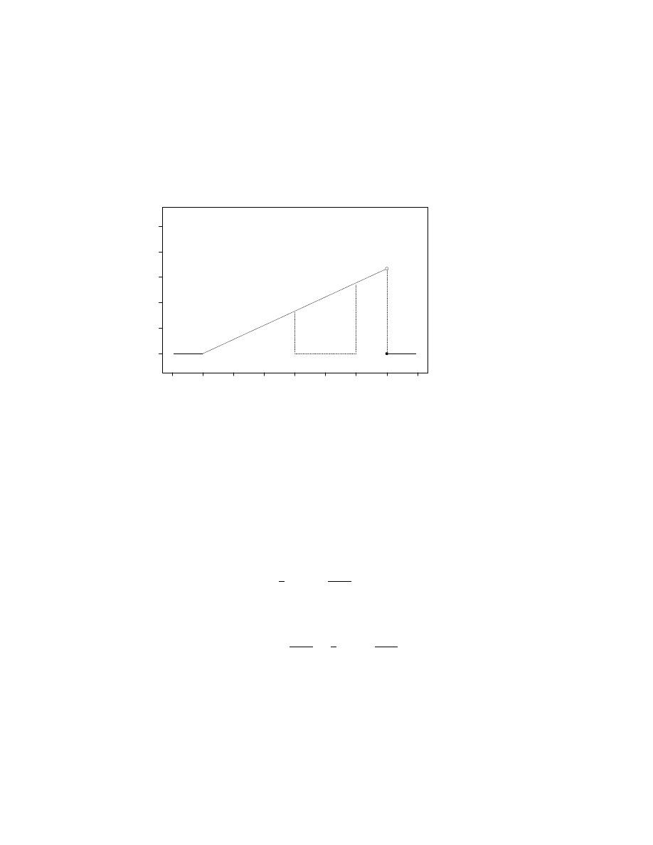
4.3. ELEMENTARY EXAMPLES
91
y
f(y)
-10
0
10
20
30
40
50
60
70
0.0
0.01
0.02
0.03
0.04
0.05
Figure 4.5: Probability Density Function for Example 2
In preparation for Example 3, we claim that the pdf of Y is
f (y) =
0
y
∈ (−∞, 0)
y/1800
y
∈ [0, 60)
0
y
∈ [60, ∞)
,
which is graphed in Figure 4.5. To check that f is really a pdf, observe that
f (y)
≥ 0 for every y ∈ < and that
Area
[0,60)
(f ) =
1
2
(60
− 0)
60
1800
= 1.
To check that f is really the pdf of Y , observe that f (y) = 0 if y
6∈ [0, 60)
and that, if y
∈ [0, 60), then
P (Y
∈ [0, y)) = P (Y ≤ y) = F (y) =
y
2
3600
=
1
2
(y
− 0)
y
1800
= Area
[0,y)
(f ).
If the pdf had been specified, then instead of deriving the cdf we would
have simply calculated
P (30 < Y < 50) = Area
(30,50)
(f )
by any of several convenient geometric arguments.

92
CHAPTER 4. CONTINUOUS RANDOM VARIABLES
Example 3
Consider two battery-powered watches. Let X
1
denote the
number of minutes past the hour at which the first watch stops and let X
2
denote the number of minutes past the hour at which the second watch stops.
What is the probability that the sum of X
1
and X
2
will be between 45 and
75?
Again we have two independent random variables, each distributed as
Uniform[0, 60), and a third random variable,
Z = X
1
+ X
2
.
We want to calculate
P (45 < Z < 75) = P (Z
∈ (45, 75)) .
z
f(z)
0
20
40
60
80
100
120
0.0
0.01
0.02
0.03
0.04
0.05
Figure 4.6: Probability Density Function for Example 3
It is apparent that Z(S) = [0, 120). Although we omit the derivation, it
can be determined mathematically that the pdf of Z is
f (z) =
0
z
∈ (−∞, 0)
z/3600
z
∈ [0, 60)
(120
− z)/3600
z
∈ [60, 120)
0
z
∈ [120, ∞)
.

4.4. NORMAL DISTRIBUTIONS
93
This pdf is graphed in Figure 4.6, in which it is apparent that the area of
the shaded region is
P (45 < Z < 75) = P (Z
∈ (45, 75)) = Area
(45,75)
(f )
= 1
−
1
2
(45
− 0)
45
3600
−
1
2
(120
− 75)
120
− 75
3600
= 1
−
45
2
60
2
=
7
16
.
4.4
Normal Distributions
We now introduce the most important family of distributions in probability
or statistics, the familiar bell-shaped curve.
Definition 4.5 A continuous random variable X is normally distributed
with mean µ and variance σ
2
> 0, denoted X
∼ Normal(µ, σ
2
), if the pdf of
X is
f (x) =
1
√
2πσ
exp
"
−
1
2
µ
x
− µ
σ
2
#
.
(4.7)
Although we will not make extensive use of (4.7), a great many useful
properties of normal distributions can be deduced directly from it. Most of
the following properties can be discerned in Figure 4.7.
1. f (x) > 0. It follows that, for any nonempty interval (a, b),
P (X
∈ (a, b)) = Area
(a,b)
(f ) > 0,
and hence that X(S) = (
−∞, +∞).
2. f is symmetric about µ, i.e. f (µ + x) = f (µ
− x).
3. f (x) decreases as
|x − µ| increases. In fact, the decrease is very rapid.
We express this by saying that f has very light tails.
4. P (µ
− σ < X < µ + σ)
.
= .68.
5. P (µ
− 2σ < X < µ + 2σ)
.
= .95.
6. P (µ
− 3σ < X < µ + 3σ)
.
= .99.
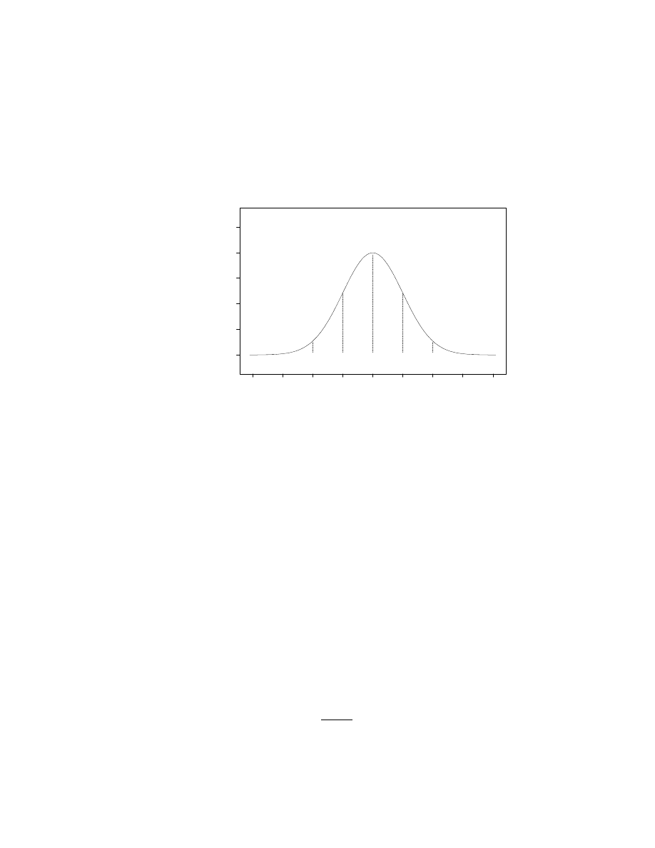
94
CHAPTER 4. CONTINUOUS RANDOM VARIABLES
x
f(x)
-4
-3
-2
-1
0
1
2
3
4
0.0
0.1
0.2
0.3
0.4
0.5
Figure 4.7: Probability Density Function of X
∼ Normal(µ, σ
2
)
Notice that there is no one normal distribution, but a 2-parameter fam-
ily of uncountably many normal distributions. In fact, if we plot µ on a
horizontal axis and σ > 0 on a vertical axis, then there is a distinct normal
distribution for each point in the upper half-plane. However, Properties 4–6
above, which hold for all choices of µ and σ, suggest that there is a funda-
mental equivalence between different normal distributions. It turns out that,
if one can compute probabilities for any one normal distribution, then one
can compute probabilities for any other normal distribution. In anticipation
of this fact, we distinguish one normal distribution to serve as a reference
distribution:
Definition 4.6 The standard normal distribution is Normal(0, 1).
The following result is of enormous practical value:
Theorem 4.1 If X
∼ Normal(µ, σ
2
), then
Z =
X
− µ
σ
∼ Normal(0, 1).

4.4. NORMAL DISTRIBUTIONS
95
The transformation Z = (X
− µ)/σ is called conversion to standard units.
Detailed tables of the standard normal cdf are widely available, as is
computer software for calculating specified values. Combined with Theorem
4.1, this availability allows us to easily compute probabilities for arbitrary
normal distributions. In the following examples, we let F denote the cdf of
Z
∼ Normal(0, 1) and we make use of the S-Plus function pnorm.
Example 1
If X
∼ Normal(1, 4), then what is the probability that X
assumes a value no more than 3?
Here, µ = 1, σ = 2, and we want to calculate
P (X
≤ 3) = P
µ
X
− µ
σ
≤
3
− µ
σ
= P
µ
Z
≤
3
− 1
2
= 1
= F (1).
We do so in S-Plus as follows:
> pnorm(1)
[1] 0.8413447
Remark
The S-Plus function pnorm accepts optional arguments that
specify a mean and standard deviation. Thus, in Example 1, we could di-
rectly evaluate P (X
≤ 3) as follows:
> pnorm(3,mean=1,sd=2)
[1] 0.8413447
This option, of course, is not available if one is using a table of the standard
normal cdf. Because the transformation to standard units plays such a
fundamental role in probability and statistics, we will emphasize computing
normal probabilities via the standard normal distribution.
Example 2
If X
∼ Normal(−1, 9), then what is the probability that X
assumes a value of at least
−7?
Here, µ =
−1, σ = 3, and we want to calculate
P (X
≥ −7) = P
µ
X
− µ
σ
≥
−7 − µ
σ
= P
µ
Z
≥
−7 + 1
3
=
−2
= 1
− P (Z < −2)
= 1
− F (−2).
We do so in S-Plus as follows:

96
CHAPTER 4. CONTINUOUS RANDOM VARIABLES
> 1-pnorm(-2)
[1] 0.9772499
Example 3
If X
∼ Normal(2, 16), then what is the probability that X
assumes a value between 0 and 10?
Here, µ = 2, σ = 4, and we want to calculate
P (0 < X < 10) = P
µ
0
− µ
σ
<
X
− µ
σ
<
10
− µ
σ
= P
µ
−.5 =
0
− 2
4
< Z <
10
− 2
4
= 2
= P (Z < 2)
− P (Z < −.5)
= F (2)
− F (−.5).
We do so in S-Plus as follows:
> pnorm(2)-pnorm(-.5)
[1] 0.6687123
Example 4
If X
∼ Normal(−3, 25), then what is the probability that
|X| assumes a value greater than 10?
Here, µ =
−3, σ = 5, and we want to calculate
P (
|X| > 10) = P (X > 10 or X < −10)
= P (X > 10) + P (X <
−10)
= P
µ
X
− µ
σ
>
10
− µ
σ
+ P
µ
X
− µ
σ
<
−10 − µ
σ
= P
µ
Z >
10 + 3
5
= 2.6
+ P
µ
Z <
−10 + 3
5
=
−1.2
= 1
− F (2.6) + F (−1.2).
We do so in S-Plus as follows:
> 1-pnorm(2.6)+pnorm(-1.2)
[1] 0.1197309
Example 5
If X
∼ Normal(4, 16), then what is the probability that X
2
assumes a value less than 36?

4.5. NORMAL SAMPLING DISTRIBUTIONS
97
Here, µ = 4, σ = 4, and we want to calculate
P (X
2
< 36) = P (
−6 < X < 6)
= P
µ
−6 − µ
σ
<
X
− µ
σ
<
6
− µ
σ
= P
µ
−2.5 =
−6 − 4
4
< Z <
6
− 4
4
= .5
= P (Z < .5)
− P (Z < −2.5)
= F (.5)
− F (−2.5).
We do so in S-Plus as follows:
> pnorm(.5)-pnorm(-2.5)
[1] 0.6852528
We defer an explanation of why the family of normal distributions is so
important until Section 6.2, concluding the present section with the following
useful result:
Theorem 4.2 If X
1
∼ Normal(µ
1
, σ
2
1
) and X
2
∼ Normal(µ
2
, σ
2
2
) are inde-
pendent, then
X
1
+ X
2
∼ Normal(µ
1
+ µ
2
, σ
2
1
+ σ
2
2
).
4.5
Normal Sampling Distributions
A number of important probability distributions can be derived by consider-
ing various functions of normal random variables. These distributions play
important roles in statistical inference. They are rarely used to describe
data; rather, they arise when analyzing data that is sampled from a normal
distribution. For this reason, they are sometimes called sampling distribu-
tions.
This section collects some definitions of and facts about several important
sampling distributions. It is not important to read this section until you
encounter these distributions in later chapters; however, it is convenient to
collect this material in one easy-to-find place.
Chi-Squared Distributions
Suppose that Z
1
, . . . , Z
n
∼ Normal(0, 1)
and consider the continuous random variable
Y = Z
2
1
+
· · · + Z
2
n
.

98
CHAPTER 4. CONTINUOUS RANDOM VARIABLES
Because each Z
2
i
≥ 0, the set of possible values of Y is Y (S) = [0, ∞). We
are interested in the distribution of Y .
The distribution of Y belongs to a family of probability distributions
called the chi-squared family. This family is indexed by a single real-valued
parameter, ν
∈ [1, ∞), called the degrees of freedom parameter. We will
denote a chi-squared distribution with ν degrees of freedom by χ
2
(ν). Figure
4.8 displays the pdfs of several chi-squared distributions.
y
f(y)
0
2
4
6
8
10
0.0
0.5
1.0
1.5
Figure 4.8: Probability Density Functions of Y
∼ χ
2
(ν) for ν = 1, 3, 5
The following fact is quite useful:
Theorem 4.3 If Z
1
, . . . , Z
n
∼ Normal(0, 1) and Y = Z
2
1
+
· · · + Z
2
n
, then
Y
∼ χ
2
(n).
In theory, this fact allows one to compute the probabilities of events defined
by values of Y , e.g. P (Y > 4.5). In practice, this requires evaluating the
cdf of χ
2
(ν), a function for which there is no simple formula. Fortunately,
there exist efficient algorithms for numerically evaluating these cdfs. The
S-Plus function pchisq returns values of the cdf of any specified chi-squared
distribution. For example, if Y
∼ χ
2
(2), then P (Y > 4.5) is

4.5. NORMAL SAMPLING DISTRIBUTIONS
99
> 1-pchisq(4.5,df=2)
[1] 0.1053992
t Distributions
Now let Z
∼ Normal(0, 1) and Y ∼ χ
2
(ν) be independent
random variables and consider the continuous random variable
T =
Z
p
Y /ν
.
The set of possible values of T is T (S) = (
−∞, ∞). We are interested in the
distribution of T .
Definition 4.7 The distribution of T is called a t distribution with ν degrees
of freedom. We will denote this distribution by t(ν).
The standard normal distribution is symmetric about the origin; i.e., if
Z
∼ Normal(0, 1), then −Z ∼ Normal(0, 1). It follows that T = Z/
p
Y /ν
and
−T = −Z/
p
Y /ν have the same distribution. Hence, if p is the pdf of
T , then it must be that p(t) = p(
−t). Thus, t pdfs are symmetric about the
origin, just like the standard normal pdf.
Figure 4.9 displays the pdfs of two t distributions. They can be dis-
tinguished by virtue of the fact that the variance of t(ν) decreases as ν
increases. It may strike you that t pdfs closely resemble normal pdfs. In
fact, the standard normal pdf is a limiting case of the t pdfs:
Theorem 4.4 Let F
ν
denote the cdf of t(ν) and let Φ denote the cdf of
Normal(0, 1). Then
lim
ν→∞
F
ν
(t) = Φ(t)
for every t
∈ (−∞, ∞).
Thus, when ν is sufficiently large (ν > 40 is a reasonable rule of thumb), t(ν)
is approximately Normal(0, 1) and probabilities involving the former can be
approximated by probabilities involving the latter.
In S-Plus, it is just as easy to calculate t(ν) probabilities as it is to
calculate Normal(0, 1) probabilities. The S-Plus function pt returns values
of the cdf of any specified t distribution. For example, if T
∼ t(14), then
P (T
≤ −1.5) is
> pt(-1.5,df=14)
[1] 0.07791266
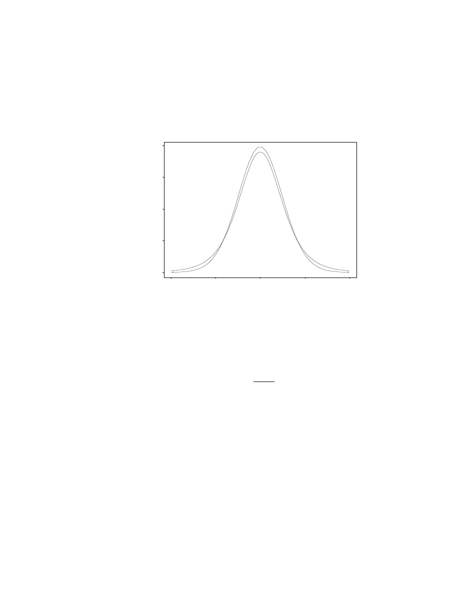
100
CHAPTER 4. CONTINUOUS RANDOM VARIABLES
y
f(y)
-4
-2
0
2
4
0.0
0.1
0.2
0.3
0.4
Figure 4.9: Probability Density Functions of T
∼ t(ν) for ν = 5, 30
F Distributions
Finally, let Y
1
∼ χ
2
(ν
1
) and Y
2
∼ χ
2
(ν
2
) be independent
random variables and consider the continuous random variable
F =
Y
1
/ν1
Y
2
/ν
2
.
Because Y
i
≥ 0, the set of possible values of F is F (S) = [0, ∞). We are
interested in the distribution of F .
Definition 4.8 The distribution of F is called an F distribution with ν
1
and ν
2
degrees of freedom. We will denote this distribution by F (ν
1
, ν
2
).
It is customary to call ν
1
the “numerator” degrees of freedom and ν
2
the
“denominator” degrees of freedom.
Figure 4.10 displays the pdfs of several F distributions.
There is an important relation between t and F distributions. To antic-
ipate it, suppose that Z
∼ Normal(0, 1) and Y
2
∼ χ
2
(ν
2
) are independent
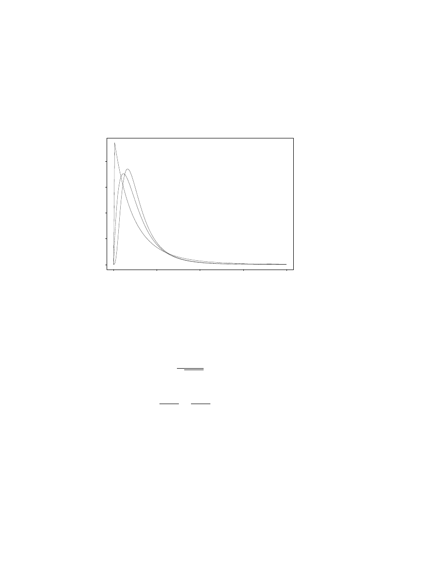
4.5. NORMAL SAMPLING DISTRIBUTIONS
101
y
f(y)
0
2
4
6
8
0.0
0.2
0.4
0.6
0.8
Figure 4.10: Probability Density Functions of F
∼ F (ν
1
, ν
2
) for ν =
(2, 12), (4, 20), (9, 10)
random variables. Then Y
1
= Z
2
∼ χ
2
(1), so
T =
Z
p
Y
2
/ν
2
∼ t (ν
2
)
and
T
2
=
Z
2
Y
2
/ν
2
=
Y
1
/1
Y
2
/ν
2
∼ F (1, ν
2
) .
More generally,
Theorem 4.5 If T
∼ t(ν), then T
2
∼ F (1, ν).
The S-Plus function pf returns values of the cdf of any specified F dis-
tribution. For example, if F
∼ F (2, 27), then P (F > 2.5) is
> 1-pf(2.5,df1=2,df2=27)
[1] 0.1008988

102
CHAPTER 4. CONTINUOUS RANDOM VARIABLES
4.6
Exercises
1. In this problem you will be asked to examine two equations. Several
symbols from each equation will be identified. Your task will be to
decide which symbols represent real numbers and which symbols rep-
resent functions. If a symbol represents a function, then you should
state the domain and the range of that function.
Recall: A function is a rule of assignment. The set of labels that the
function might possibly assign is called the range of the function; the
set of objects to which labels are assigned is called the domain. For
example, when I grade your test, I assign a numeric value to your
name. Grading is a function that assigns real numbers (the range) to
students (the domain).
(a) In the equation p = P (Z > 1.96), please identify each of the
following symbols as a real number or a function:
i. p
ii. P
iii. Z
(b) In the equation σ
2
= E (X
− µ)
2
, please identify each of the fol-
lowing symbols as a real number or a function:
i. σ
ii. E
iii. X
iv. µ
2. Suppose that X is a continuous random variable with probability den-
sity function (pdf) f defined as follows:
f (x) =
0
if x < 1
2(x
− 1) if 1 ≤ x ≤ 2
0
if x > 2
.
(a) Graph f .
(b) Verify that f is a pdf.
(c) Compute P (1.50 < X < 1.75).

4.6. EXERCISES
103
3. Consider the function f :
< → < defined by
f (x) =
0
x < 0
cx
0 < x < 1.5
c(3
− x)
1.5 < x < 3
0
x > 3
,
where c is an undetermined constant.
(a) For what value of c is f a probability density function?
(b) Suppose that a continuous random variable X has probability
density function f . Compute EX. (Hint: Draw a picture of the
pdf.)
(c) Compute P (X > 2).
(d) Suppose that Y
∼ Uniform(0, 3). Which random variable has the
larger variance, X or Y ? (Hint: Draw a picture of the two pdfs.)
(e) Graph the cumulative distribution function of X.
4. Let X be a normal random variable with mean µ =
−5 and standard
deviation σ = 10. Compute the following:
(a) P (X < 0)
(b) P (X > 5)
(c) P (
−3 < X < 7)
(d) P (
|X + 5| < 10)
(e) P (
|X − 3| > 2)

104
CHAPTER 4. CONTINUOUS RANDOM VARIABLES

Chapter 5
Quantifying Population
Attributes
The distribution of a random variable is a mathematical abstraction of the
possible outcomes of an experiment. Indeed, having identified a random
variable of interest, we will often refer to its distribution as the population. If
one’s goal is to represent an entire population, then one can hardly do better
than to display its entire probability mass or density function. Usually,
however, one is interested in specific attributes of a population. This is true
if only because it is through specific attributes that one comprehends the
entire population, but it is also easier to draw inferences about a specific
population attribute than about the entire population. Accordingly, this
chapter examines several population attributes that are useful in statistics.
We will be especially concerned with measures of centrality and mea-
sures of dispersion. The former provide quantitative characterizations of
where the “middle” of a population is located; the latter provide quanti-
tative characterizations of how widely the population is spread. We have
already introduced one important measure of centrality, the expected value
of a random variable (the population mean, µ), and one important measure
of dispersion, the standard deviation of a random variable (the population
standard deviation, σ). This chapter discusses these measures in greater
depth and introduces other, complementary measures.
5.1
Symmetry
We begin by considering the following question:
105

106
CHAPTER 5. QUANTIFYING POPULATION ATTRIBUTES
Where is the “middle” of a normal distribution?
It is quite evident from Figure 4.7 that there is only one plausible answer to
this question: if X
∼ Normal(µ, σ
2
), then the “middle” of the distribution
of X is µ.
Let f denote the pdf of X. To understand why µ is the only plausible
middle of f , recall a property of f that we noted in Section 4.4: for any x,
f (µ + x) = f (µ
− x). This property states that f is symmetric about µ. It is
the property of symmetry that restricts the plausible locations of “middle”
to the central value µ.
To generalize the above example of a measure of centrality, we introduce
an important qualitative property that a population may or may not possess:
Definition 5.1 Let X be a continuous random variable with probability den-
sity function f . If there exists a value θ
∈ < such that
f (θ + x) = f (θ
− x)
for every x
∈ <, then X is a symmetric random variable and θ is its center
of symmetry.
We have already noted that X
∼ Normal(µ, σ
2
) has center of symmetry µ.
Another example of symmetry is illustrated in Figure 5.1: X
∼ Uniform[a, b]
has center of symmetry (a + b)/2.
For symmetric random variables, the center of symmetry is the only
plausible measure of centrality—of where the “middle” of the distribution
is located. Symmetry will play an important role in our study of statistical
inference. Our primary concern will be with continuous random variables,
but the concept of symmetry can be used with other random variables as
well. Here is a general definition:
Definition 5.2 Let X be a random variable. If there exists a value θ
∈ <
such that the random variables X
− θ and θ − X have the same distribution,
then X is a symmetric random variable and θ is its center of symmetry.
Suppose that we attempt to compute the expected value of a symmetric
random variable X with center of symmetry θ. Thinking of the expected
value as a weighted average, we see that each θ + x will be weighted precisely
as much as the corresponding θ
− x. Thus, if the expect value exists (there
are a few pathological random variables for which the expected value is
undefined), then it must equal the center of symmetry, i.e. EX = θ. Of
course, we have already seen that this is the case for X
∼ Normal(µ, σ
2
) and
for X
∼ Uniform[a, b].

5.2. QUANTILES
107
x
f(x)
Figure 5.1: X
∼ Uniform[a, b] has center of symmetry (a + b)/2.
5.2
Quantiles
In this section we introduce population quantities that can be used for a
variety of purposes. As in Section 5.1, these quantities are most easily un-
derstood in the case of continuous random variables:
Definition 5.3 Let X be a continuous random variable and let α
∈ (0, 1).
If q = q(X; α) is such that P (X < q) = α and P (X > q) = 1
− α, then q is
called an α quantile of X.
If we express the probabilities in Definition 5.3 as percentages, then we see
that q is the 100α percentile of the distribution of X.
Example 1
Suppose that X
∼ Uniform[a, b] has pdf f, depicted in
Figure 5.2. Then q is the value in (a, b) for which
α = P (X < q) = Area
[a,q]
(f ) = (q
− a) ·
1
b
− a
,
i.e. q = a + α(b
− a). This expression is easily interpreted: to the lower
endpoint a, add 100α% of the distance b
− a to obtain the 100α percentile.

108
CHAPTER 5. QUANTIFYING POPULATION ATTRIBUTES
x
f(x)
Figure 5.2: A quantile of a Uniform distribution.
Example 2
Suppose that X has pdf
f (x) =
(
x/2 x
∈ [0, 2]
0
otherwise
)
,
depicted in Figure 5.3. Then q is the value in (0, 2) for which
α = P (X < q) = Area
[a,q]
(f ) =
1
2
· (q − 0) ·
µ
q
2
− 0
=
q
2
4
,
i.e. q = 2α.
Example 3
Suppose that X
∼ Normal(0, 1) has cdf F . Then q is the
value in (
−∞, ∞) for which α = P (X < q) = F (q), i.e. q = F
−1
(α). Unlike
the previous examples, we cannot compute q by elementary calculations.
Fortunately, the S-Plus function qnorm computes quantiles of normal distri-
butions. For example, we compute the α = 0.95 quantile of X as follows:
> qnorm(.95)
[1] 1.644854
5.2. QUANTILES
109
x
f(x)
-0.5
0.0
0.5
1.0
1.5
2.0
2.5
0.0
0.2
0.4
0.6
0.8
1.0
Figure 5.3: A quantile of another distribution.
Example 4
Suppose that X has pdf
f (x) =
(
1/2 x
∈ [0, 1] ∪ [2, 3]
0
otherwise
)
,
depicted in Figure 5.4. Notice that P (X
∈ [0, 1]) = 0.5 and P (X ∈ [2, 3]) =
0.5. If α
∈ (0, 0.5), then we can use the same reasoning that we employed
in Example 1 to deduce that q = 2α. Similarly, if α
∈ (0.5, 1), then q =
2+2(α
−0.5) = 2α+1. However, if α = 0.5, then we encounter an ambiguity:
the equalities P (X < q) = 0.5 and P (X > q) = 0.5 hold for any q
∈ [1, 2].
Accordingly, any q
∈ [1, 2] is an α = 0.5 quantile of X. Thus, quantiles are
not always unique.
To avoid confusion when a quantile are not unique, it is nice to have a
convention for selecting one of the possible quantile values. In the case that
α = 0.5, there is a universal convention:
Definition 5.4 The midpoint of the interval of all values of the α = 0.5
quantile is called the population median.
110
CHAPTER 5. QUANTIFYING POPULATION ATTRIBUTES
x
f(x)
-1
0
1
2
3
4
0.0
0.2
0.4
0.6
0.8
1.0
Figure 5.4: A distribution for which the α = 0.5 quantile is not unique.
In Example 4, the population median is q = 1.5.
Working with the quantiles of a continuous random variable X is straight-
forward because P (X = q) = 0 for any choice of q. This means that
P (X < q) + P (X > q) = 1; hence, if P (X < q) = α, then P (X > q) = 1
− α.
Furthermore, it is always possible to find a q for which P (X < q) = α. This
is not the case if X is discrete.
Example 5
Let X be a discrete random variable that assumes values
in the set
{1, 2, 3} with probabilities p(1) = 0.4, p(2) = 0.4, and p(3) = 0.2.
What is the median of X?
Imagine accumulating probability as we move from
−∞ to ∞. At what
point do we find that we have acquired half of the total probability? The
answer is that we pass from having 40% of the probability to having 80% of
the probability as we occupy the point q = 2. It makes sense to declare this
value to be the median of X.
Here is another argument that appeals to Definition 5.3. If q < 2, then
P (X > q) = 0.6 > 0.5. Hence, it would seem that the population median
should not be less than 2. Similarly, if q > 2, then P (X < q) = 0.8 > 0.5.

5.2. QUANTILES
111
Hence, it would seem that the population median should not be greater than
2. We conclude that the population median should equal 2. But notice that
P (X < 2) = 0.4 < 0.5 and P (X > 2) = 0.2 < 0.5! We conclude that
Definition 5.3 will not suffice for discrete random variables. However, we
can generalize the reasoning that we have just employed as follows:
Definition 5.5 Let X be a random variable and let α
∈ (0, 1). If q =
q(X; α) is such that P (X < q)
≤ α and P (X > q) ≤ 1 − α, then q is called
an α quantile of X.
The remainder of this section describes how quantiles are often used to
measure centrality and dispersion. The following three quantiles will be of
particular interest:
Definition 5.6 Let X be a random variable. The first, second, and third
quartiles of X, denoted q
1
(X), q
2
(X), and q
3
(X), are the α = 0.25, α = 0.50,
and α = 0.75 quantiles of X. The second quartile is also called the median
of X.
5.2.1
The Median of a Population
If X is a symmetric random variable with center of symmetry θ, then
P (X < θ) = P (X > θ) =
1
− P (X = θ)
2
≤
1
2
and q
2
(X) = θ. Even if X is not symmetric, the median of X is an excellent
way to define the “middle” of the population. Many statistical procedures
use the median as a measure of centrality.
Example 6
One useful property of the median is that it is rather in-
sensitive to the influence of extreme values that occur with small probability.
For example, let X
k
denote a discrete random variable that assumes values
in
{−1, 0, 1, 10
k
} for n = 1, 2, 3, . . .. Suppose that X
k
has the following pmf:
x p
k
(x)
−1
0.19
0
0.60
1
0.19
10
k
0.02

112
CHAPTER 5. QUANTIFYING POPULATION ATTRIBUTES
Most of the probability (98%) is concentrated on the values
{−1, 0, 1}. This
probability is centered at x = 0. A small amount of probability is con-
centrated at a large value, x = 10, 100, 1000, . . .. If we want to treat these
large values as aberrations (perhaps our experiment produces a physically
meaningful value x
∈ {−1, 0, 1} with probability 0.98, but our equipment
malfunctions and produces a physically meaningless value x = 10
k
with
probability 0.02), then we might prefer to declare that x = 0 is the central
value of X. In fact, no matter how large we choose k, the median refuses to
be distracted by the aberrant value: P (X < 0) = 0.19 and P (X > 0) = 0.21,
so the median of X is q
2
(X) = 0.
5.2.2
The Interquartile Range of a Population
Now we turn our attention from the problem of measuring centrality to the
problem of measuring dispersion. Can we use quantiles to quantify how
widely spread are the values of a random variable? A natural approach is
to choose two values of α and compute the corresponding quantiles. The
distance between these quantiles is a measure of dispersion.
To avoid comparing apples and oranges, let us agree on which two values
of α we will choose. Statisticians have developed a preference for α = 0.25
and α = 0.75, in which case the corresponding quantiles are the first and
third quartiles.
Definition 5.7 Let X be a random variable with first and third quartiles q
1
and q
3
. The interquartile range of X is the quantity
iqr(X) = q
3
− q
1
.
If X is a continuous random variable, then P (q
1
< X < q
3
) = 0.5, so the
interquartile range is the interval of values on which is concentrated the
central 50% of the probability.
Like the median, the interquartile range is rather insensitive to the in-
fluence of extreme values that occur with small probability. In Example 6,
the central 50% of the probability is concentrated on the single value x = 0.
Hence, the interquartile range is 0
− 0 = 0, regardless of where the aberrant
2% of the probability is located.
5.3
The Method of Least Squares
Let us return to the case of a symmetric random variable X, in which case
the “middle” of the distribution is unambiguously the center of symmetry

5.3. THE METHOD OF LEAST SQUARES
113
θ. Given this measure of centrality, how might we construct a measure of
dispersion? One possibility is to measure how far a “typical” value of X
lies from its central value, i.e. to compute E
|X − θ|. This possibility leads
to several remarkably fertile approaches to describing both dispersion and
centrality.
Given a designated central value c and another value x, we say that the
absolute deviation of x from c is
|x − c| and that the squared deviation of x
from c is (x
− c)
2
. The magnitude of a typical absolute deviation is E
|X − c|
and the magnitude of a typical squared deviation is E(X
− c)
2
. A natural
approach to measuring centrality is to choose a value of c that typically
results in small deviations, i.e. to choose c either to minimize E
|X − c| or
to minimize E(X
− c)
2
. The second possibility is a simple example of the
method of least squares.
Measuring centrality by minimizing the magnitude of a typical absolute
or squared deviation results in two familiar quantities:
Theorem 5.1 Let X be a random variable with population median q
2
and
population mean µ = EX. Then
1. The value of c that minimizes E
|X − c| is c = q
2
.
2. The value of c that minimizes E(X
− c)
2
is c = µ.
It follows that medians are naturally associated with absolute deviations
and that means are naturally associated with squared deviations. Having
discussed the former in Section 5.2.1, we now turn to the latter.
5.3.1
The Mean of a Population
Imagine creating a physical model of a probability distribution by distribut-
ing weights along the length of a board. The location of the weights are the
values of the random variable and the weights represent the probabilities of
those values. After gluing the weights in place, we position the board atop
a fulcrum. How must the fulcrum be positioned in order that the board be
perfectly balanced? It turns out that one should position the fulcrum at the
mean of the probability distribution. For this reason, the expected value of
a random variable is sometimes called its center of mass.
Thus, like the population median, the population mean has an appealing
interpretation that commends its use as a measure of centrality. If X is a
symmetric random variable with center of symmetry θ, then µ = EX = θ
and q
2
= q
2
(X) = θ, so the population mean and the population median

114
CHAPTER 5. QUANTIFYING POPULATION ATTRIBUTES
agree. In general, this is not the case. If X is not symmetric, then one should
think carefully about whether one is interested in the population mean and
the population median. Of course, computing both measures and examining
the discrepancy between them may be highly instructive. In particular, if
EX
6= q
2
(X), then X is not a symmetric random variable.
In Section 5.2.1 we noted that the median is rather insensitive to the
influence of extreme values that occur with small probability. The mean
lacks this property. In Example 6,
EX
k
=
−0.19 + 0.00 + 0.19 + 10
k
· 0.02 = 2 · 10
k−2
,
which equals 0.2 if k = 1, 2 if k = 2, 20 if k = 3, 200 if k = 4, and so on.
No matter how reluctantly, the population mean follows the aberrant value
toward infinity as k increases.
5.3.2
The Standard Deviation of a Population
Suppose that X is a random variable with EX = µ and Var X = σ
2
. If we
adopt the method of least squares, then we obtain c = µ as our measure
of centrality, in which case the magnitude of a typical squared deviation is
E(X
− µ)
2
= σ
2
, the population variance. The variance measures dispersion
in squared units. For example, if X measures length in meters, then Var X
is measured in meters squared. If, as in Section 5.2.2, we prefer to measure
dispersion in the original units of measurement, then we must take the square
root of the variance. Accordingly, we will emphasize the population standard
deviation, σ, as a measure of dispersion.
Just as it is natural to use the median and the interquartile range to-
gether, so is it natural to use the mean and the standard deviation together.
In the case of a symmetric random variable, the median and the mean agree.
However, the interquartile range and the standard deviation measure disper-
sion in two fundamentally different ways. To gain insight into their relation
to each other, suppose that X
∼ Normal(0, 1), in which case the population
standard deviation is σ = 1. We use S-Plus to compute iqr(X):
> qnorm(.75)-qnorm(.25)
[1] 1.34898
We have derived a useful fact: the interquartile range of a normal random
variable is approximately 1.35 standard deviations. If we encounter a random
variable for which this is not the case, then that random variable is not
normally distributed.

5.4. EXERCISES
115
Like the mean, the standard deviation is sensitive to the influence of
extreme values that occur with small probability. Consider Example 6. The
variance of X
k
is
σ
2
k
= EX
2
k
− (EX
k
)
2
=
³
0.19 + 0.00 + 0.19 + 100
k
· 0.02
´
−
³
2
· 10
k−2
´
2
= 0.38 + 2
· 100
k−1
− 4 · 100
k−2
= 0.38 + 196
· 100
k−2
,
so σ
1
=
√
2.34, σ
2
=
√
196.38, σ
3
=
√
19600.38, and so on. The population
standard deviation tends toward infinity as the aberrant value tends toward
infinity.
5.4
Exercises
1. Refer to the random variable X defined in Exercise 1 of Chapter 4.
Compute q
2
(X), the population median, and iqr(X), the population
interquartile range.
2. Consider the function g :
< → < defined by
g(x) =
0
x < 0
x
x
∈ [0, 1]
1
x
∈ [1, 2]
3
− x
x
∈ [2, 3]
0
x > 3
.
Let f (x) = cg(x), where c is an undetermined constant.
(a) For what value of c is f a probability density function?
(b) Suppose that a continuous random variable X has probability
density function f . Compute P (1.5 < X < 2.5).
(c) Compute EX.
(d) Let F denote the cumulative distribution function of X. Compute
F (1).
(e) Determine the .90 quantile of f .
3. Identify each of the following statements as True or False. Briefly
explain each of your answers.
(a) For every symmetric random variable X, the median of X equals
the average of the first and third quartiles of X.

116
CHAPTER 5. QUANTIFYING POPULATION ATTRIBUTES
(b) For every random variable X, the interquartile range of X is
greater than the standard deviation of X.
(c) For every random variable X, the expected value of X lies between
the first and third quartile of X.
(d) If the standard deviation of a random variable equals zero, then
so does its interquartile range.
(e) If the median of a random variable equals its expected value, then
the random variable is symmetric.
4. For each of the following random variables, discuss whether the median
or the mean would be a more useful measure of centrality:
(a) The annual income of U.S. households.
(b) The lifetime of 75-watt light bulbs.
5. The S-Plus function qbinom returns quantiles of the binomial distri-
bution. For example, quartiles of X
∼ Binomial(n = 3; p = 0.5) can
be computed as follows:
> alpha <- c(.25,.5,.75)
> qbinom(alpha,size=3,prob=.5)
[1] 1 1 2
Notice that X is a symmetric random variable with center of symmetry
θ = 1.5, but pbinom computes q
2
(X) = 1. This reveals that S-Plus
may produce unexpected results when it computes the quantiles of
discrete random variables. By experimenting with various choices of
n and p, try to discover a rule according to which pbinom computes
quartiles of the binomial distribution.

Chapter 6
Sums and Averages of
Random Variables
In this chapter we will describe one important way in which the theory
of probability provides a foundation for statistical inference. Imagine an
experiment that can be performed, independently and identically, as many
times as we please. We describe this situation by supposing the existence
of a sequence of independent and identically distributed random variables,
X
1
, X
2
, . . ., and we assume that these random variables have a finite mean
µ = EX
i
and a finite variance σ
2
= Var X
i
.
This chapter is concerned with the behavior of certain random variables
that can be constructed from X
1
, X
2
, . . .. Specifically, let
¯
X
n
=
1
n
n
X
i=1
X
i
.
The random variable ¯
X
n
is the average, or sample mean, of the random
variables X
1
, . . . , X
n
. We are interested in what the behavior of ¯
X
n
, the
sample mean, tells us about µ, the population mean.
By definition, EX
i
= µ. Thus, the population mean is the average value
assumed by the random variable X
i
. This statement is also true of the
sample mean:
E ¯
X
n
=
1
n
n
X
i=1
EX
i
=
1
n
n
X
i=1
µ = µ;
however, there is a crucial distinction between X
i
and ¯
X
n
.
117

118 CHAPTER 6. SUMS AND AVERAGES OF RANDOM VARIABLES
The tendency of a random variable to assumee a value that is close to
its expected value is quantified by computing its variance. By definition,
Var X
i
= σ
2
, but
Var ¯
X
n
= Var
Ã
1
n
n
X
i=1
X
i
!
=
1
n
2
n
X
i=1
Var X
i
=
1
n
2
n
X
i=1
σ
2
=
σ
2
n
.
Thus, the sample mean has less variability than any of the individual random
variables that are being averaged. Averaging decreases variation. Further-
more, as n
→ ∞, Var ¯
X
n
→ 0. Thus, by repeating our experiment enough
times, we can make the variation in the sample mean as small as we please.
The preceding remarks suggest that, if the population mean is unknown,
then we can draw inferences about it by observing the behavior of the sample
mean. This fundamental insight is the basis for a considerable portion of
this book. The remainder of this chapter refines the relation between the
population mean and the behavior of the sample mean.
6.1
The Weak Law of Large Numbers
Recall Definition 1.12 from Section 1.4: a sequence of real numbers
{y
n
}
converges to a limit c
∈ < if, for every ² > 0, there exits a natural number
N such that y
n
∈ (c − ², c + ²) for each n ≥ N. Our first task is to generalize
from convergence of a sequence of real numbers to convergence of a sequence
of random variables.
If we replace
{y
n
}, a sequence of real numbers, with {Y
n
}, a sequence of
random variables, then the event that Y
n
∈ (c − ², c + ²) is uncertain. Rather
than demand that this event must occur for n sufficiently large, we ask only
that the probability of this event tend to unity as n tends to infinity. This
results in
Definition 6.1 A sequence of random variables
{Y
n
} converges in probabil-
ity to a constant c, written Y
n
P
→ c, if, for every ² > 0,
lim
n→∞
P (Y
n
∈ (c − ², c + ²)) = 1.
Convergence in probability is depicted in Figure 6.1 using the pdfs of con-
tinuous random variables. (One could also use the pmfs of discrete random
variables.) We see that
p
n
= P (Y
n
∈ (c − ², c + ²)) =
Z
c+²
c−²
f
n
(x) dx

6.1. THE WEAK LAW OF LARGE NUMBERS
119
Figure 6.1: Convergence in Probability
is tending to unity as n increases. Notice, however, that each p
n
< 1.
The concept of convergence in probability allows us to state an important
result.
Theorem 6.1 (Weak Law of Large Numbers) Let X
1
, X
2
, . . . be any se-
quence of independent and identically distributed random variables having
finite mean µ and finite variance σ
2
. Then
¯
X
n
P
→ µ.
This result is of considerable consequence. It states that, as we average more
and more X
i
, the average values that we observe tend to be distributed closer
and closer to the theoretical average of the X
i
. This property of the sample
mean strengthens our contention that the behavior of ¯
X
n
provides more and
more information about the value of µ as n increases.
The Weak Law of Large Numbers (WLLN) has an important special
case.
Corollary 6.1 (Law of Averages) Let A be any event and consider a se-
quence of independent and identical experiments in which we observe whether

120 CHAPTER 6. SUMS AND AVERAGES OF RANDOM VARIABLES
or not A occurs. Let p = P (A) and define independent and identically dis-
tributed random variables by
X
i
=
(
1 A occurs
0 A
c
occurs
)
.
Then X
i
∼ Bernoulli(p), ¯
X
n
is the observed frequency with which A occurs
in n trials, and µ = EX
i
= p = P (A) is the theoretical probability of A.
The WLLN states that the former tends to the latter as the number of trials
increases.
The Law of Averages formalizes our common experience that “things
tend to average out in the long run.” For example, we might be surprised
if we tossed a fair coin n = 10 times and observed ¯
X
10
= .9; however, if we
knew that the coin was indeed fair (p = .5), then we would remain confident
that, as n increased, ¯
X
n
would eventually tend to .5.
Notice that the conclusion of the Law of Averages is the frequentist
interpretation of probability. Instead of defining probability via the notion
of long-run frequency, we defined probability via the Kolmogorov axioms.
Although our approach does not require us to interpret probabilities in any
one way, the Law of Averages states that probability necessarily behaves in
the manner specified by frequentists.
6.2
The Central Limit Theorem
The Weak Law of Large Numbers states a precise sense in which the dis-
tribution of values of the sample mean collapses to the population mean as
the size of the sample increases. As interesting and useful as this fact is, it
leaves several obvious questions unanswered:
1. How rapidly does the sample mean tend toward the population mean?
2. How does the shape of the sample mean’s distribution change as the
sample mean tends toward the population mean?
To answer these questions, we convert the random variables in which we are
interested to standard units.
We have supposed the existence of a sequence of independent and iden-
tically distributed random variables, X
1
, X
2
, . . ., with finite mean µ = EX
i
and finite variance σ
2
= Var X
i
. We are interested in the sum and/or the

6.2. THE CENTRAL LIMIT THEOREM
121
average of X
1
, . . . , X
n
. It will be helpful to identify several crucial pieces of
information for each random variable of interest:
random
expected
standard
standard
variable
value
deviation
units
X
i
µ
σ
(X
i
− µ) /σ
P
n
i=1
X
i
nµ
√
n σ
(
P
n
i=1
X
i
− nµ) ÷ (
√
n σ)
¯
X
n
µ
σ/
√
n
¡
¯
X
n
− µ
¢
÷ (σ/
√
n)
First we consider X
i
. Notice that converting to standard units does
not change the shape of the distribution of X
i
.
For example, if X
i
∼
Bernoulli(0.5), then the distribution of X
i
assigns equal probability to each
of two values, x = 0 and x = 1. If we convert to standard units, then the
distribution of
Z
1
=
X
i
− µ
σ
=
X
i
− 0.5
0.5
also assigns equal probability to each of two values, z
1
=
−1 and z
1
= 1. In
particular, notice that converting X
i
to standard units does not automati-
cally result in a normally distributed random variable.
Next we consider the sum and the average of X
1
, . . . , X
n
. Notice that,
after converting to standard units, these quantities are identical:
Z
n
=
P
n
i=1
X
i
− nµ
√
nσ
=
(1/n)
(1/n)
P
n
i=1
X
i
− nµ
√
n σ
=
¯
X
n
− µ
σ/
√
n
.
It is this new random variable on which we shall focus our attention.
We begin by observing that
Var
£
√
n
¡
¯
X
n
− µ
¢¤
= Var (σZ
n
) = σ
2
Var (Z
n
) = σ
2
is constant. The WLLN states that
¡
¯
X
n
− µ
¢
P
→ 0,
so
√
n is a “magnification factor” that maintains random variables with a
constant positive variance. We conclude that 1/
√
n measures how rapidly
the sample mean tends toward the population mean.

122 CHAPTER 6. SUMS AND AVERAGES OF RANDOM VARIABLES
Now we turn to the more refined question of how the distribution of
the sample mean changes as the sample mean tends toward the population
mean. By converting to standard units, we are able to distinguish changes in
the shape of the distribution from changes in its mean and variance. Despite
our inability to make general statements about the behavior of Z
1
, it turns
out that we can say quite a bit about the behavior of Z
n
as n becomes large.
The following theorem is one of the most remarkable and useful results in
all of mathematics. It is fundamental to the study of both probability and
statistics.
Theorem 6.2 (Central Limit Theorem) Let X
1
, X
2
, . . . be any sequence of
independent and identically distributed random variables having finite mean
µ and finite variance σ
2
. Let
Z
n
=
¯
X
n
− µ
σ/
√
n
,
let F
n
denote the cdf of Z
n
, and let Φ denote the cdf of the standard normal
distribution. Then, for any fixed value z
∈ <,
P (Z
n
≤ z) = F
n
(z)
→ Φ(z)
as n
→ ∞.
The Central Limit Theorem (CLT) states that the behavior of the average
(or, equivalently, the sum) of a large number of independent and identically
distributed random variables will resemble the behavior of a standard normal
random variable. This is true regardless of the distribution of the random
variables that are being averaged. Thus, the CLT allows us to approximate
a variety of probabilities that otherwise would be intractable. Of course, we
require some sense of how many random variables must be averaged in order
for the normal approximation to be reasonably accurate. This does depend
on the distribution of the random variables, but a popular rule of thumb is
that the normal approximation can be used if n
≥ 30. Often, the normal
approximation works quite well with even smaller n.
Example 1
A chemistry professor is attempting to determine the con-
formation of a certain molecule. To measure the distance between a pair of
nearby hydrogen atoms, she uses NMR spectroscopy. She knows that this
measurement procedure has an expected value equal to the actual distance
and a standard deviation of 0.5 angstroms. If she replicates the experiment

6.2. THE CENTRAL LIMIT THEOREM
123
36 times, then what is the probability that the average measured value will
fall within 0.1 angstroms of the true value?
Let X
i
denote the measurement obtained from replication i, for i =
1, . . . , 36. We are told that µ = EX
i
is the actual distance between the
atoms and that σ
2
= Var X
i
= 0.5
2
. Let Z
∼ Normal(0, 1). Then, applying
the CLT,
P
¡
µ
− 0.1 < ¯
X
36
< µ + 0.1
¢
= P
¡
µ
− 0.1 − µ < ¯
X
36
− µ < µ + 0.1 − µ
¢
= P
Ã
−0.1
0.5/6
<
¯
X
36
− µ
0.5/6
<
0.1
0.5/6
!
= P (
−1.2 < Z
n
< 1.2)
.
= P (
−1.2 < Z < 1.2)
= Φ(1.2)
− Φ(−1.2).
Now we use S-Plus:
> pnorm(1.2)-pnorm(-1.2)
[1] 0.7698607
We conclude that there is a chance of approximately 77% that the average
of the measured values will fall with 0.1 angstroms of the true value.
Notice that it is not possible to compute the exact probability. To do so
would require knowledge of the distribution of the X
i
.
It is sometimes useful to rewrite the normal approximations derived from
the CLT as statements of the approximate distributions of the sum and the
average. For the sum we obtain
n
X
i=1
X
i
·
∼ Normal
³
nµ, nσ
2
´
(6.1)
and for the average we obtain
¯
X
n
·
∼ Normal
Ã
µ,
σ
2
n
!
.
(6.2)
These approximations are especially useful when combined with Theorem
4.2.

124 CHAPTER 6. SUMS AND AVERAGES OF RANDOM VARIABLES
Example 2
The chemistry professor in Example 1 asks her graduate
student to replicate the experiment that she performed an additional 64 times.
What is the probability that the averages of their respective measured values
will fall within 0.1 angstroms of each other?
The professor’s measurements are
X
1
, . . . , X
36
∼
³
µ, 0.5
2
´
.
Applying (6.2), we obtain
¯
X
36
·
∼ Normal
µ
µ,
0.25
36
.
Similarly, the student’s measurements are
Y
1
, . . . , Y
64
∼
³
µ, 0.5
2
´
.
Applying (6.2), we obtain
¯
Y
64
·
∼ Normal
µ
µ,
0.25
64
or
− ¯
Y
64
·
∼ Normal
µ
−µ,
0.25
64
.
Now we apply Theorem 4.2 to conclude that
¯
X
36
− ¯
Y
64
= ¯
X
36
+
¡
− ¯
Y
64
¢
·
∼ Normal
Ã
0,
0.25
36
+
0.25
64
=
5
2
48
2
!
.
Converting to standard units, it follows that
P
¡
−0.1 < ¯
X
36
− ¯
Y
64
< 0.1
¢
= P
Ã
−0.1
5/48
<
¯
X
36
− ¯
Y
64
5/48
<
0.1
5/48
!
.
= P (
−0.96 < Z < 0.96)
= Φ(0.96)
− Φ(−0.96).
Now we use S-Plus:
> pnorm(.96)-pnorm(-96)
[1] 0.6629448
We conclude that there is a chance of approximately 66% that the two av-
erages will fall with 0.1 angstroms of each other.

6.2. THE CENTRAL LIMIT THEOREM
125
The CLT has a long history. For the special case of X
i
∼ Bernoulli(p),
a version of the CLT was obtained by De Moivre in the 1730s. The first
attempt at a more general CLT was made by Laplace in 1810, but definitive
results were not obtained until the second quarter of the 20th century. The-
orem 6.2 is actually a very special case of far more general results established
during that period. However, with one exception to which we now turn, it
is sufficiently general for our purposes.
The astute reader may have noted that, in Examples 1 and 2, we assumed
that the population mean µ was unknown but that the population variance
σ
2
was known. Is this plausible? In Examples 1 and 2, it might be that
the nature of the instrumentation is sufficiently well understood that the
population variance may be considered known. In general, however, it seems
somewhat implausible that we would know the population variance and not
know the population mean.
The normal approximations employed in Examples 1 and 2 require knowl-
edge of the population variance. If the variance is not known, then it must
be estimated from the measured values. Chapters 7 and 8 will introduce
procedures for doing so. In anticipation of those procedures, we state the
following generalization of Theorem 6.2:
Theorem 6.3 Let X
1
, X
2
, . . . be any sequence of independent and identi-
cally distributed random variables having finite mean µ and finite variance
σ
2
. Suppose that D
1
, D
2
, . . . is a sequence of random variables with the prop-
erty that D
2
n
P
→ σ
2
and let
T
n
=
¯
X
n
− µ
D
n
/
√
n
.
Let F
n
denote the cdf of T
n
, and let Φ denote the cdf of the standard normal
distribution. Then, for any fixed value t
∈ <,
P (T
n
≤ t) = F
n
(t)
→ Φ(t)
as n
→ ∞.
We conclude this section with a warning. Statisticians usually invoke
the CLT in order to approximate the distribution of a sum or an average
of random variables X
1
, . . . , X
n
that are observed in the course of an ex-
periment. The X
i
need not be normally distributed themselves—indeed,
the grandeur of the CLT is that it does not assume normality of the X
i
.
Nevertheless, we will discover that many important statistical procedures

126 CHAPTER 6. SUMS AND AVERAGES OF RANDOM VARIABLES
do assume that the X
i
are normally distributed. Researchers who hope to
use these procedures naturally want to believe that their X
i
are normally
distributed. Often, they look to the CLT for reassurance. Many think
that, if only they replicate their experiment enough times, then somehow
their observations will be drawn from a normal distribution. This is ab-
surd! Suppose that a fair coin is tossed once. Let X
1
denote the number
of Heads, so that X
1
∼ Bernoulli(0.5). The Bernoulli distribution is not at
all like a normal distribution. If we toss the coin one million times, then
each X
i
∼ Bernoulli(0.5). The Bernoulli distribution does not miraculously
become a normal distribution. Remember,
The Central Limit Theorem does not say that a large sample was
necessarily drawn from a normal distribution!
On some occasions, it is possible to invoke the CLT to anticipate that the
random variable to be observed will behave like a normal random variable.
This involves recognizing that the observed random variable is the sum or the
average of lots of independent and identically distributed random variables
that are not observed.
Example 3
To study the effect of an insect growth regulator (IGR) on
termite appetite, an entomologist plans an experiment. Each replication of
the experiment will involve placing 100 ravenous termites in a container with
a dried block of wood. The block of wood will be weighed before the experiment
begins and after a fixed number of days. The random variable of interest is
the decrease in weight, the amount of wood consumed by the termites. Can
we anticipate the distribution of this random variable?
The total amount of wood consumed is the sum of the amounts con-
sumed by each termite. Assuming that the termites behave independently
and identically, the CLT suggests that this sum should be approximately
normally distributed.
When reasoning as in Example 3, one should construe the CLT as no
more than suggestive. Most natural processes are far too complicated to
be modelled so simplistically with any guarantee of accuracy. One should
always examine the observed values to see if they are consistent with one’s
theorizing. The next chapter will introduce several techniques for doing
precisely that.

6.3. EXERCISES
127
6.3
Exercises
1. Suppose that I toss a fair coin 100 times and observe 60 Heads. Now
I decide to toss the same coin another 100 times. Does the Law of
Averages imply that I should expect to observe another 40 Heads?
2. Chris owns a laser pointer that is powered by two AAAA batteries. A
pair of batteries will power the pointer for an average of five hours
use, with a standard deviation of 30 minutes. Chris decides to take
advantage of a sale and buys 20 2-packs of AAAA batteries. What is
the probability that he will get to use his laser pointer for at least 105
hours before he needs to buy more batteries?
3. A certain financial theory posits that daily fluctuations in stock prices
are independent random variables. Suppose that the daily price fluc-
tuations (in dollars) of a certain blue-chip stock are independent and
identically distributed random variables X
1
, X
2
, X
3
, . . ., with EX
i
=
0.01 and Var X
i
= 0.01. (Thus, if today’s price of this stock is $50,
then tomorrow’s price is $50 + X
1
, etc.) Suppose that the daily price
fluctuations (in dollars) of a certain internet stock are independent and
identically distributed random variables Y
1
, Y
2
, Y
3
, . . ., with EY
j
= 0
and Var Y
j
= 0.25.
Now suppose that both stocks are currently selling for $50 per share
and you wish to invest $50 in one of these two stocks for a period of 50
market days. Assume that the costs of purchasing and selling a share
of either stock are zero.
(a) Approximate the probability that you will make a profit on your
investment if you purchase a share of the blue-chip stock.
(b) Approximate the probability that you will make a profit on your
investment if you purchase a share of the internet stock.
(c) Approximate the probability that you will make a profit of at
least $20 if you purchase a share of the blue-chip stock.
(d) Approximate the probability that you will make a profit of at
least $20 if you purchase a share of the internet stock.
(e) Approximate the probability that, after 400 days, the price of the
internet stock will exceed the price of the blue-chip stock.

128 CHAPTER 6. SUMS AND AVERAGES OF RANDOM VARIABLES

Chapter 7
Data
Experiments are performed for the purpose of obtaining information about a
population that is imperfectly understood. Experiments produce data, the
raw material from which statistical procedures draw inferences about the
population under investigation.
The probability distribution of a random variable X is a mathematical
abstraction of an experimental procedure for sampling from a population.
When we perform the experiment, we observe one of the possible values of
X. To distinguish an observed value of a random variable from the ran-
dom variable itself, we designate random variables by uppercase letters and
observed values by corresponding lowercase letters.
Example 1
A coin is tossed and Heads is observed. The mathematical
abstraction of this experiment is X
∼ Bernoulli(p) and the observed value
of X is x = 1.
We will be concerned with experiments that are replicated a fixed number
of times. By replication, we mean that each repetition of the experiment is
performed under identical conditions and that the repetitions are mutually
independent. Mathematically, we write X
1
, . . . , X
n
∼ P . Let x
i
denote the
observed value of X
i
. The set of observed values, ~x =
{x
1
, . . . , x
n
}, is called
a sample.
This chapter introduces several useful techniques for extracting informa-
tion from samples. This information will be used to draw inferences about
populations (for example, to guess the value of the population mean) and
to assess assumptions about populations (for example, to decide whether
or not the population can plausibly be modelled by a normal distribution).
129

130
CHAPTER 7. DATA
Drawing inferences about population attributes (especially means) is the pri-
mary subject of subsequent chapters, which will describe specific procedures
for drawing specific types of inferences. However, deciding which procedure
is appropriate often involves assessing the validity of certain statistical as-
sumptions. The methods described in this chapter will be our primary tools
for making such assessments.
To assess whether or not an assumption is plausible, one must be able
to investigate what happens when the assumption holds. For example, if
a scientist needs to decide whether or not it is plausible that her sample
was drawn from a normal distribution, then she needs to be able to rec-
ognize normally distributed data. For this reason, the samples studied in
this chapter were generated under carefully controlled conditions, by com-
puter simulation. This allows us to investigate how samples drawn from
specified distributions should behave, thereby providing a standard against
which to compare experimental data for which the true distribution can nev-
er be known. Fortunately, S-Plus provides several convenient functions for
simulating random sampling.
Example 2
Consider the experiment of tossing a fair die n = 20 times.
We can simulate this experiment as follows:
> SampleSpace <- c(1,2,3,4,5,6)
> sample(x=SampleSpace,size=20,replace=T)
[1] 1 6 3 2 2 3 5 3 6 4 3 2 5 3 2 2 3 2 4 2
Example 3
Consider the experiment of drawing a sample of size n = 5
from Normal(2, 3). We can simulate this experiment as follows:
> rnorm(5,mean=2,sd=sqrt(3))
[1] 1.3274812 0.5901923 2.5881013 1.2222812 3.4748139
7.1
The Plug-In Principle
We will employ a general methodology for relating samples to populations.
In Chapters 2–6 we developed a formidable apparatus for studying popu-
lations (probability distributions). We would like to exploit this apparatus
fully. Given a sample, we will pretend that the sample is a finite population
(discrete probability distribution) and then we will use methods for studying
finite populations to learn about the sample. This approach is sometimes
called the Plug-In Principle.

7.1. THE PLUG-IN PRINCIPLE
131
The Plug-In Principle employs a fundamental construction:
Definition 7.1 Let ~x = (x
1
, . . . , x
n
) be a sample. The empirical proba-
bility distribution associated with ~x, denoted ˆ
P
n
, is the discrete probability
distribution defined by assigning probability 1/n to each
{x
i
}.
Notice that, if a sample contains several copies of the same numerical value,
then each copy is assigned probability 1/n. This is illustrated in the following
example.
Example 2 (continued)
A fair die is rolled n = 20 times, resulting
in the sample
~x =
{1, 6, 3, 2, 2, 3, 5, 3, 6, 4, 3, 2, 5, 3, 2, 2, 3, 2, 4, 2}.
(7.1)
The empirical distribution ˆ
P
20
is the discrete distribution that assigns the
following probabilities:
x
i
#
{x
i
} ˆ
P
20
(
{x
i
})
1
1
0.05
2
7
0.35
3
6
0.30
4
2
0.10
5
2
0.10
6
2
0.10
Notice that, although the true probabilities are P (
{x
i
}) = 1/6, the empirical
probabilities range from .05 to .35. The fact that ˆ
P
20
differs from P is
an example of sampling variation. Statistical inference is concerned with
determining what the empirical distribution (the sample) tells us about the
true distribution (the population).
The empirical distribution, ˆ
P
n
, is an appealing way to approximate the
actual probability distribution, P , from which the sample was drawn. Notice
that the empirical probability of any event A is just
ˆ
P
n
(A) = #
{x
i
∈ A} ·
1
n
,
the observed frequency with which A occurs in the sample. By the Law of
Averages, this quantity tends to the true probability of A as the size of the

132
CHAPTER 7. DATA
sample increases. Thus, the theory of probability provides a mathematical
justification for approximating P with ˆ
P
n
when P is unknown.
Because the empirical distribution is an authentic probability distribu-
tion, all of the methods that we developed for studying (discrete) distribu-
tions are available for studying samples. For example,
Definition 7.2 The empirical cdf, usually denoted ˆ
F
n
, is the cdf associated
with ˆ
P
n
, i.e.
ˆ
F
n
(y) = ˆ
P
n
(X
≤ y) =
#
{x
i
≤ y}
n
.
The empirical cdf of sample (7.1) is graphed in Figure 7.1.
y
F(y)
-2
-1
0
1
2
3
4
5
6
7
8
9
0.0
0.2
0.4
0.6
0.8
1.0
Figure 7.1: An Empirical CDF
7.2
Plug-In Estimates of Mean and Variance
Population quantities defined by expected values are easily estimated by the
plug-in principle. For example, suppose that X
1
, . . . , X
n
∼ P and that we

7.2. PLUG-IN ESTIMATES OF MEAN AND VARIANCE
133
observe a sample ~x =
{x
1
, . . . , x
n
}. Let µ = EX
i
denote the population
mean. Then
Definition 7.3 The plug-in estimate of µ, denoted ˆ
µ
n
, is the mean of the
empirical distibution:
ˆ
µ
n
=
n
X
i=1
x
i
·
1
n
=
1
n
n
X
i=1
x
i
= ¯
x
n
.
This quantity is called the sample mean.
Example 2 (continued)
The population mean is
µ = EX
i
= 1
·
1
6
+2
·
1
6
+3
·
1
6
+4
·
1
6
+5
·
1
6
+6
·
1
6
=
1 + 2 + 3 + 4 + 5 + 6
6
= 3.5.
The sample mean of sample (7.1) is
ˆ
µ
20
= ¯
x
20
= 1
·
1
20
+ 6
·
1
20
+
· · · + 4 ·
1
20
+ 2
·
1
20
= 1
× 0.05 + 2 × 0.35 + 3 × 0.30 + 4 × 0.10 +
5
× 0.10 + 6 × 0.10
= 3.15.
Notice that ˆ
µ
20
6= µ. This is another example of sampling variation.
The variance can be estimated in the same way. Let σ
2
= Var X
i
denote
the population variance; then
Definition 7.4 The plug-in estimate of σ
2
, denoted
c
σ
2
n
, is the variance of
the empirical distribution:
c
σ
2
n
=
n
X
i=1
(x
i
− ˆµ
n
)
2
·
1
n
=
1
n
n
X
i=1
(x
i
− ¯x
n
)
2
=
1
n
n
X
i=1
x
2
i
−
Ã
1
n
n
X
i=1
x
i
!
2
.
Notice that we do not refer to
c
σ
2
n
as the sample variance. As will be discussed
in Section 8.2.2, most authors designate another, equally plausible estimate
of the population variance as the sample variance.

134
CHAPTER 7. DATA
Example 2 (continued)
The population variance is
σ
2
= EX
2
i
− (EX
i
)
2
=
1
2
+ 2
2
+ 3
2
+ 4
2
+ 5
2
+ 6
2
6
− 3.5
2
=
35
12
.
= 2.9167.
The plug-in estimate of the variance is
d
σ
2
20
=
³
1
2
× 0.05 + 2
2
× 0.35 + 3
2
× 0.30+
4
2
× 0.10 + 5
2
× 0.10 + 6
2
× 0.10
´
− 3.15
2
= 1.9275.
Again, notice that
d
σ
2
20
6= σ
2
, yet another example of sampling variation.
7.3
Plug-In Estimates of Quantiles
Population quantities defined by quantiles can also be estimated by the plug-
in principle. Again, suppose that X
1
, . . . , X
n
∼ P and that we observe a
sample ~x =
{x
1
, . . . , x
n
}. Then
Definition 7.5 The plug-in estimate of a population quantile is the corre-
sponding quantile of the empirical distribution. In particular, the sample
median is the median of the empirical distribution. The sample interquartile
range is the interquartile range of the empirical distribution.
Example 4
Consider the experiment of drawing a sample of size n = 20
from Uniform(1, 5). This probability distribution has a population median
of 3 and a population interquartile range of 4
− 2 = 2. We simulated this
experiment (and listed the sample in increasing order) with the following
S-Plus command:
> x <- sort(runif(20,min=1,max=5))
This resulted in the following sample:
1.124600 1.161286 1.445538 1.828181 1.853359
1.934939 1.943951 2.107977 2.372500 2.448152
2.708874 3.297806 3.418913 3.437485 3.474940
3.698471 3.740666 4.039637 4.073617 4.195613
The sample median is
2.448152 + 2.708874
2
= 2.578513.

7.3. PLUG-IN ESTIMATES OF QUANTILES
135
Notice that the sample median does not exactly equal the population median.
To compute the sample interquartile range, we require the first and
third sample quartiles, i.e. the α = 0.25 and α = 0.75 sample quantiles.
We must now confront the fact that Definition 5.5 may not specify unique
quantile values. For the empirical distribution of the sample above, any
number in [1.853359, 1.934939] is a sample first quartile and any number in
[3.474940, 3.698471] is a sample third quartile.
The statistical community has not agreed on a convention for resolving
the ambiguity in the definition of quartiles. One natural and popular possi-
bility is to use the central value in each interval of possible quartiles. If we
adopt that convention here, then the sample interquartile range is
3.474940 + 3.698471
2
−
1.853359 + 1.934939
2
= 1.692556.
S-Plus adopts a slightly different convention. The following command
computes several useful sample quantities:
> summary(x)
Min.
1st Qu.
Median
Mean
3rd Qu.
Max.
1.124600 1.914544 2.578513 2.715325 3.530823 4.195613
If we use these values of the first and third sample quartiles, then the sample
interquartile range is 3.530823
− 1.914544 = 1.616279.
Notice that the sample quantities do not exactly equal the population
quantities that they estimate, regardless of which convention we adopt for
defining quartiles.
Used judiciously, sample quantiles can be extremely useful when trying
to discern various features of the population from which the sample was
drawn. The remainder of this section describes two graphical techniques for
assimilating and displaying sample quantile information.
7.3.1
Box Plots
Information about sample quartiles is often displayed visually, in the form
of a box plot. A box plot of a sample consists of a rectangle that extends
from the first to the third sample quartile, thereby drawing attention to the
central 50% of the data. Thus, the length of the rectangle equals the sample
interquartile range. The location of the sample median is also identified, and
its location within the rectangle often provides insight into whether or not

136
CHAPTER 7. DATA
the population from which the sample was drawn is symmetric. Whiskers
extend from the ends of the rectangle, either to the extreme values of the
data or to 1.5 times the sample interquartile range, whichever is less. Values
that lie beyond the whiskers are called outliers and are individually identified
by additional lines.
0
2
4
6
8
10
Figure 7.2: Box Plot of a Sample from χ
2
(3)
Example 5
The pdf of the asymmetric distribution χ
2
(3) was graphed
in Figure 4.8. The following S-Plus commands draw a random sample of
n = 100 observed values from this population, then construct a box plot of
the sample:
> x <- rchisq(100,df=3)
> boxplot(x)
An example of a box plot produced by these commands is displayed in Figure
7.2. In this box plot, the numerical values in the sample are represented by
the vertical axis.
The third quartile of the box plot in Figure 7.2 is farther above the
median than the first quartile is below it. The short lower whisker extends

7.3. PLUG-IN ESTIMATES OF QUANTILES
137
from the first quartile to the minimal value in the sample, whereas the long
upper whisker extends 1.5 interquartile ranges beyond the third quartile.
Furthermore, there are 4 outliers beyond the upper whisker. Once we learn
to discern these key features of the box plot, we can easily recognize that
the population from which the sample was drawn is not symmetric.
The frequency of outliers in a sample often provides useful diagnostic
information. Recall that, in Section 5.3, we computed that the interquartile
range of a normal distribution is 1.34898. A value is an outlier if it lies more
than
z =
1.34898
2
+ 1.5
· 1.34898 = 2.69796
standard deviations from the mean. Hence, the probability that an observa-
tion drawn from a normal distribution is an outlier is
> 2*pnorm(-2.69796)
[1] 0.006976582
and we would expect a sample drawn from a normal distribution to contain
approximately 7 outliers per 1000 observations. A sample that contains a
dramatically different proportion of outliers, as in Example 5, is not likely
to have been drawn from a normal distribution.
Box plots are especially useful for comparing several populations.
Example 6
We drew samples of 100 observations from three normal
populations: Normal(0, 1), Normal(2, 1), and Normal(1, 4). To attempt to
discern in the samples the various differences in population mean and stan-
dard deviation, we examined side-by-side box plots. This was accomplished
by the following S-Plus commands:
> z1 <- rnorm(100)
> z2 <- rnorm(100,mean=2,sd=1)
> z3 <- rnorm(100,mean=1,sd=2)
> boxplot(z1,z2,z3)
An example of the output of these commands is displayed in Figure 7.3.
7.3.2
Normal Probability Plots
Another powerful graphical technique that relies on quantiles are quantile-
quantile (QQ) plots, which plot the quantiles of one distribution against the
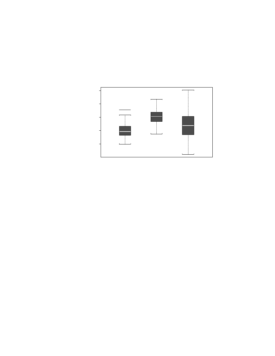
138
CHAPTER 7. DATA
-2
0
2
4
6
Figure 7.3: Box Plots of Samples from Three Normal Distributions
quantiles of another. QQ plots are used to compare the shapes of two distri-
butions, most commonly by plotting the observed quantiles of an empirical
distribution against the corresponding quantiles of a theoretical normal dis-
tribution. In this case, a QQ plot is often called a normal probability plot. If
the shape of the empirical distribution resembles a normal distribution, then
the points in a normal probability plot should tend to fall on a straight line.
If they do not, then we should be skeptical that the sample was drawn from
a normal distribution. Extracting useful information from normal probabil-
ity plots requires some practice, but the patient data analyst will be richly
rewarded.
Example 4 (continued)
A normal probability plot of the sample gen-
erated in Example 5 against a theoretical normal distribution is displayed in
Figure 7.4. This plot was created using the following S-Plus command:
> qqnorm(x)
Notice the systematic and asymmetric bending away from linearity in this
plot. In particular, the smaller quantiles are much closer to the central values

7.3. PLUG-IN ESTIMATES OF QUANTILES
139
•
•
•
•
•
•
•
•
•
•
•
•
•
•
•
•
•
•
•
•
•
•
•
•
•
•
•
•
•
•
•
•
•
•
•
•
•
•
•
•
•
•
•
•
•
•
•
•
•
•
•
•
•
•
•
•
•
•
•
•
•
•
•
•
•
•
•
•
•
•
•
•
•
•
•
•
•
•
•
•
•
•
•
•
•
•
•
•
•
•
•
•
•
•
•
•
•
•
•
•
Quantiles of Standard Normal
book.data.chisq3
-2
-1
0
1
2
0
2
4
6
8
10
Figure 7.4: Normal Probability Plot of a Sample from χ
2
(3)
than should be the case for a normal distribution. This suggests that this
sample was drawn from a nonnormal distribution that is skewed to the right.
Of course, we know that this sample was drawn from χ
2
(3), which is in fact
skewed to the right.
When using normal probability plots, one must guard against overinter-
preting slight departures from linearity. Remember: some departures from
linearity will result from sampling variation. Consequently, before drawing
definitive conclusions, the wise data analyst will generate several random
samples from the theoretical distribution of interest in order to learn how
much sampling variation is to be expected. Before dismissing the possibil-
ity that the sample in Example 5 was drawn from a normal distribution,
one should generate several normal samples of the same size for comparison.
The normal probability plots of four such samples are displayed in Figure
7.5. In none of these plots did the points fall exactly on a straight line.
However, upon comparing the normal probability plot in Figure 7.4 to the
normal probability plots in Figure 7.5, it is abundantly clear that the sample
in Example 5 was not drawn from a normal distribution.

140
CHAPTER 7. DATA
•
•
•
•
•
•
•
•
• •
•
•
•
•
•
•
•
•
•
•
•
•
•
•
• ••
•
•
•
•
•
•
•
•
•
•
•
•
•
•
••
•
•
•
•
•
••
•
•
•
•
•
•
•
• •
•
• •
• •
••
•
•
•
•
•
•
•
•
•
•
• •
•
• •
•
•
•
•
•
•
•
•
•
•
• •
•
•
•
•
•
• •
Quantiles of Standard Normal
z1
-2
-1
0
1
2
-2
0
1
2
3
••
•
•
•
••
•
•
•
•
•
•
•
•
•
•
•
•
•
•
•
•
•
•
•
•
•
•
•
•
•
•
•
•
•
•
•
•
•
•
•
•
••
•
•
•
•
•
•
•
•
•
•
•
•
•
•
•
•
•
•
•
•
•
•
•
•
•
•
•
•
•
•
•
•
•
•
•
••
•
•
•
•
•
•
•
•
•
•
•
•
•
•
•
•
•
•
Quantiles of Standard Normal
z2
-2
-1
0
1
2
-2
0
1
2
•
•
•
•
•
•
•
•
•
•
•
•
•
•
•
•
••
•
•
•
•
•
•
•
••
•
• •
•
•
•
•
•
•
•
•
•
•
•
•
• •
•
•
•
•
•
•
•
•
•••
•
•
•
•
•
•
•
•
•
•
•
•
•
•
•
•
•
• •
•
•
•
•
•
•
•
•
•
•
•
•
••
•
•
•
•
•
•
•
• •
•
•
•
Quantiles of Standard Normal
z3
-2
-1
0
1
2
-3
-1
1
2
•
•
•
•
•
•
•
•
•
•
•
•
•
• •
••
•
•
•
•
•
•
•
•
•
•
•
•
•
•
•
•
•
•
•
•
•
•
•
•
•
•
•
•
•
•
•
•
•
•
•
••
•
•
•
•
•
•
•
•
•
•
•
•
•
•
•
•
••
•
•
•
•
•
•
•
••
•
•
•
•
•
•
•
•
•
•
•
•
•
•
•
•
•
•
•
Quantiles of Standard Normal
z4
-2
-1
0
1
2
-4
-2
0
1
2
Figure 7.5: Normal Probability Plots of Four Samples from Normal(0, 1)
7.4
Density Estimates
Suppose that ~x =
{x
1
, . . . , x
n
} is a sample drawn from an unknown pdf f.
Box plots and normal probability plots are extremely useful graphical tech-
niques for discerning in ~x certain important attributes of f , e.g. centrality,
dispersion, asymmetry, nonnormality. To discern more subtle features of f ,
we now ask if it is possible to reconstruct from ~x a pdf ˆ
f
n
that approximates
f . This is a difficult problem, one that remains a vibrant topic of research
and about which little is said in introductory courses. However, using the
concept of the empirical distribution, one can easily motivate one of the most
popular techniques for nonparametric probability density estimation.
The logic of the empirical distribution is this: by assigning probability
1/n to each x
i
, one accumulates more probability in regions that produced
more observed values. However, because the entire amount 1/n is placed
exactly on the value x
i
, the resulting empirical distribution is necessarily
discrete. If the population from which the sample was drawn is discrete,
then the empirical distribution estimates the probability mass function. But
if the population from which the sample was drawn is continuous, then all

7.4. DENSITY ESTIMATES
141
possible values occur with zero probability. In this case, there is nothing
special about the precise values that were observed—what is important are
the regions in which they occurred.
Instead of placing all of the probability 1/n assigned to x
i
exactly on the
value x
i
, we now imagine distributing it in a neighborhood of x
i
according
to some probability density function. This construction will also result in
more probability accumulating in regions that produced more values, but it
will produce a pdf instead of a pmf. Here is a general description of this
approach, usually called kernel density estimation:
1. Choose a probability density function K, the kernel. Typically, K is a
symmetric pdf centered at the origin. Common choices of K include
the Normal(0, 1) and Uniform[
−0.5, 0.5] pdfs.
2. At each x
i
, center a rescaled copy of the kernel. This pdf,
1
h
K
µ
x
− x
i
h
,
(7.2)
will control the distribution of the 1/n probability assigned to x
i
. The
parameter h is variously called the smoothing parameter, the window
width, or the bandwidth.
3. The difficult decision in constructing a kernel density estimate is the
choice of h. The technical details of this issue are beyond the scope of
this book, but the underlying principles are quite simple:
• Small values of h mean that the standard deviation of (7.2) will be
small, so that the 1/n probability assigned to x
i
will be distributed
close to x
i
. This is appropriate when n is large and the x
i
are
tightly packed.
• Large values of h mean that the standard deviation of (7.2) will
be large, so that the 1/n probability assigned to x
i
will be widely
distributed in the general vicinity of x
i
. This is appropriate when
n is small and the x
i
are sparse.
4. After choosing K and h, the kernel density estimate of f is
ˆ
f
n
(x) =
n
X
i=1
1
n
1
h
K
µ
x
− x
i
h
=
1
nh
n
X
i=1
K
µ
x
− x
i
h
.
Such estimates are easily computed and graphed using the S-Plus func-
tions density and plot.
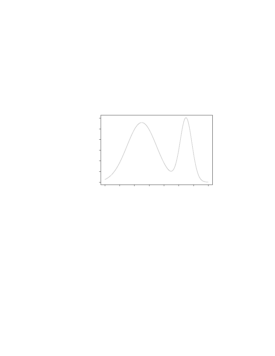
142
CHAPTER 7. DATA
Example 7
Consider the probability density function f displayed in
Figure 7.6. The most striking feature of f is that it is bimodal. Can we
detect this feature using a sample drawn from f ?
x
f(x)
-3
-2
-1
0
1
2
3
4
0.0
0.05
0.10
0.15
0.20
0.25
0.30
Figure 7.6: A Bimodal Probability Density Function
We drew a sample of size n = 100 from f . A box plot and a normal
probability plot of this sample are displayed in Figure 7.7. It is difficult to
discern anything unusual from the box plot. The normal probability plot
contains all of the information in the sample, but it is encoded in such a way
that the feature of interest is not easily extracted. In contrast, the kernel
density estimate displayed in Figure 7.8 clearly reveals that the sample was
drawn from a bimodal population. After storing the sample in the vector x,
this estimate was computed and plotted using the following S-Plus command:
> plot(density(x),type="b")

7.5. EXERCISES
143
-3
-2
-1
0
1
2
3
•
•
•
•
••
••
••••
••••
•••
•••••
•••
••
•••
••••
••••
•••
•••
•••
•
•••
••••
••
•••••
•••
•
•
•••
••
•••••
•••
••••
••
••
•••
••••
• •
•
Quantiles of Standard Normal
x
-2
-1
0
1
2
-3
-2
-1
0
1
2
3
Figure 7.7: Box Plot and Normal Probability Plot for Example 7
7.5
Exercises
1. The following independent samples were drawn from four populations:
Sample 1 Sample 2 Sample 3 Sample 4
5.098
4.627
3.021
7.390
2.739
5.061
6.173
5.666
2.146
2.787
7.602
6.616
5.006
4.181
6.250
7.868
4.016
3.617
1.875
2.428
9.026
3.605
6.996
6.740
4.965
6.036
4.850
7.605
5.016
4.745
6.661
10.868
6.195
2.340
6.360
1.739
4.523
6.934
7.052
1.996
(a) Use the boxplot function to create side-by-side box plots of these
samples. Does it appear that these samples were all drawn from
the same population? Why or why not?

144
CHAPTER 7. DATA
• • • •
•
•
•
•
•
•
•
•
•
•
•
•
•
•
•
• • •
•
•
•
•
•
•
•
•
•
•
•
•
•
•
•
• •
•
•
•
•
•
•
•
•
• • •
density(x)$x
density(x)$y
-4
-2
0
2
4
0.0
0.05
0.10
0.15
0.20
0.25
Figure 7.8: A Kernel Density Estimate for Example 7
(b) Use the rnorm function to draw four independent samples, each
of size n = 10, from one normal distribution. Examine box plots
of these samples. Is it possible that Samples 1–4 were all drawn
from the same normal distribution?
2. The following sample, ~x, was collected and sorted:
0.246 0.327 0.423 0.425 0.434
0.530 0.583 0.613 0.641 1.054
1.098 1.158 1.163 1.439 1.464
2.063 2.105 2.106 4.363 7.517
(a) Graph the empirical cdf of ~x.
(b) Calculate the plug-in estimates of the mean, the variance, the
median, and the interquartile range.
(c) Take the square root of the plug-in estimate of the variance and
compare it to the plug-in estimate of the interquartile range. Do
you think that ~x was drawn from a normal distribution? Why or
why not?

7.5. EXERCISES
145
(d) Use the qqnorm function to create a normal probability plot. Do
you think that ~x was drawn from a normal distribution? Why or
why not?
(e) Now consider the transformed sample ~y produced by replacing
each x
i
with its natural logarithm. If ~x is stored in the vector x,
then ~y can be computed by the following S-Plus command:
> y <- log(x)
Do you think that ~y was drawn from a normal distribution? Why
or why not?
3. Forty-one students taking Math 308 (Applied Statistics) at the College
of William & Mary were administered a test. The following test scores
were observed and sorted:
90 90 89 88 85 85 84 82 82 82
81 81 81 80 79 79 78 76 75 74
72 71 70 66 65 63 62 62 61 59
58 58 57 56 56 53 48 44 40 35 33
(a) Do these numbers appear to be a random sample from a normal
distribution?
(b) Does this list of numbers have any interesting anomalies?
4. Experiment with using S-Plus to generate simulated random samples
of various sizes. Use the summary function to compute the quartiles of
these samples. Try to discern the convention that this function uses to
define sample quartiles.

146
CHAPTER 7. DATA

Chapter 8
Inference
In Chapters 2–6 we developed methods for studying the behavior of ran-
dom variables.
Given a specific probability distribution, we can calcu-
late the probabilities of various events. For example, knowing that Y
∼
Binomial(n = 100; p = .5), we can calculate P (40
≤ Y ≤ 60). Roughly
speaking, statistics is concerned with the opposite sort of problem. For ex-
ample, knowing that Y
∼ Binomial(n = 100; p), where the value of p is
unknown, and having observed Y = y (say y = 32), what can we say about
p? The phrase statistical inference describes any procedure for extracting
information about a probability distribution from an observed sample.
The present chapter introduces the fundamental principles of statistical
inference. We will discuss three types of statistical inference—point esti-
mation, hypothesis testing, and set estimation—in the context of drawing
inferences about a single population mean. More precisely, we will consider
the following situation:
1. X
1
, . . . , X
n
are independent and identically distributed random vari-
ables. We observe a sample, ~x =
{x
1
, . . . , x
n
}.
2. EX
i
= µ and Var X
i
= σ
2
<
∞. We are interested in drawing in-
ferences about the population mean µ, a quantity that is fixed but
unknown.
3. The sample size, n, is sufficiently large that we can use the normal
approximation provided by the Central Limit Theorem.
We begin, in Section 8.1, by examining a narrative that is sufficiently
nuanced to motivate each type of inferential technique. We then proceed to
147

148
CHAPTER 8. INFERENCE
discuss point estimation (Section 8.2), hypothesis testing (Sections 8.3 and
8.4), and set estimation (Section 8.5). Although we are concerned exclusively
with large-sample inferences about a single population mean, it should be
appreciated that this concern often arises in practice. More importantly,
the fundamental concepts that we introduce in this context are common to
virtually all problems that involve statistical inference.
8.1
A Motivating Example
We consider an artificial example that permits us to scrutinize the precise
nature of statistical reasoning. Two siblings, a magician (Arlen) and an at-
torney (Robin) agree to resolve their disputed ownership of an Ert´e painting
by tossing a penny. Just as Robin is about to toss the penny in the air, Arlen
suggests that spinning the penny on a table will ensure better randomiza-
tion. Robin assents and spins the penny. As it spins, Arlen calls “Tails!”
The penny comes to rest with Tails facing up and Arlen takes possession
of the Ert´e.
That evening, Robin wonders if she has been had. She decides to perform
an experiment. She spins the same penny on the same table 100 times and
observes 68 Tails. It occurs to Robin that perhaps spinning the penny was
not entirely fair, but she is reluctant to accuse her brother of impropriety
until she is convinced that the results of her experiment cannot be dismissed
as coincidence. How should she proceed?
It is easy to devise a mathematical model of Robin’s experiment: each
spin of the penny is a Bernoulli trial and the experiment is a sequence of
n = 100 trials. Let X
i
denote the outcome of spin i, where X
i
= 1 if Heads is
observed and X
i
= 0 if Tails is observed. Then X
1
, . . . , X
100
∼ Bernoulli(p),
where p is the fixed but unknown (to Robin!) probability that a single
spin will result in Heads. The probability distribution Bernoulli(p) is our
mathematical abstraction of a population and the population parameter of
interest is µ = EX
i
= p, the population mean.
Let
Y =
100
X
i=1
X
i
,
the total number of Heads obtained in n = 100 spins. Under the mathe-
matical model that we have proposed, Y
∼ Binomial(p). In performing her

8.1. A MOTIVATING EXAMPLE
149
experiment, Robin observes a sample ~x =
{x
1
, . . . , x
100
} and computes
y =
100
X
i=1
x
i
,
the total number of Heads in her sample. In our narrative, y = 32.
We emphasize that p
∈ [0, 1] is fixed but unknown. Robin’s goal is to
draw inferences about this fixed but unknown quantity. We consider three
questions that she might ask:
1. What is the true value of p? More precisely, what is a reasonable guess
as to the true value of p?
2. Is p = .5? Specifically, is the evidence that p
6= .5 so compelling that
Robin can comfortably accuse Arlen of impropriety?
3. What are plausible values of p? In particular, is there a subset of [0, 1]
that Robin can confidently claim contains the true value of p?
The first set of questions introduces a type of inference that statisticians
call point estimation. We have already encountered (in Chapter 7) a natural
approach to point estimation, the plug-in principle. In the present case, the
plug-in principle suggests estimating the theoretical probability of success,
p, by computing the observed proportion of successes,
ˆ
p =
y
n
=
32
100
= .32.
The second set of questions introduces a type of inference that statis-
ticians call hypothesis testing. Having calculated ˆ
p = .32
6= .5, Robin is
inclined to guess that p
6= .5. But how compelling is the evidence that
p
6= .5? Let us play devil’s advocate: perhaps p = .5, but chance produced
“only” y = 32 instead of a value nearer EY = np = 100
× .5 = 50. This
is a possibility that we can quantify. If Y
∼ Binomial(n = 100; p = .5),
then the probability that Y will deviate from its expected value by at least
|50 − 32| = 18 is
P
= P (
|Y − 50| ≥ 18)
= P (Y
≤ 32 or Y ≥ 68)
= P (Y
≤ 32) + P (Y ≥ 68)
= P (Y
≤ 32) + 1 − P (Y ≤ 67)
= pbinom(32,100,.5)+1-pbinom(67,100,.5)
= 0.0004087772.

150
CHAPTER 8. INFERENCE
This significance probability seems fairly small—perhaps small enough to
convince Robin that in fact p
6= .5.
The third set of questions introduces a type of inference that statisticians
call set estimation. We have just tested the possibility that p = p
0
in the
special case p
0
= .5. Now, imagine testing the possibility that p = p
0
for
each p
0
∈ [0, 1]. Those p
0
that are not rejected as inconsistent with the
observed data, y = 32, will constitute a set of plausible values of p.
To implement this procedure, Robin will have to adopt a standard of
implausibility. Perhaps she decides to reject p
0
as implausible when the
corresponding significance probability,
P
= P (
|Y − 100p
0
| ≥ |32 − 100p
0
|)
= P (Y
− 100p
0
≥ |32 − 100p
0
|) + P (Y − 100p
0
≤ −|32 − 100p
0
|)
= P (Y
≥ 100p
0
+
|32 − 100p
0
|) + P (Y ≤ 100p
0
− |32 − 100p
0
|) ,
satisfies P
≤ .1. Using the S-Plus function pbinom, some trial and error
reveals that P > .10 if p
0
lies in the interval [.245, .404]. (The endpoints of
this interval are included.) Notice that this interval does not contain p
0
= .5,
which we had already rejected as implausible.
8.2
Point Estimation
The goal of point estimation is to make a reasonable guess of the unknown
value of a designated population quantity, e.g. the population mean. The
quantity that we hope to guess is called the estimand.
8.2.1
Estimating a Population Mean
Suppose that the estimand is µ, the population mean. The plug-in principle
suggests estimating µ by computing the mean of the empirical distribution.
This leads to the plug-in estimate of µ, ˆ
µ = ¯
x
n
. Thus, we estimate the mean
of the population by computing the mean of the sample, which is certainly
a natural thing to do.
We will distinguish between
¯
x
n
=
1
n
n
X
i=1
x
i
,

8.2. POINT ESTIMATION
151
a real number that is calculated from the sample ~x =
{x
1
, . . . , x
n
}, and
¯
X
n
=
1
n
n
X
i=1
X
i
,
a random variable that is a function of the random variables X
1
, . . . , X
n
.
(Such a random variable is called a statistic.) The latter is our rule for
guessing, an estimation procedure or estimator. The former is the guess
itself, the result of applying our rule for guessing to the sample that we
observed, an estimate.
The quality of an individual estimate depends on the individual sample
from which it was computed and is therefore affected by chance variation.
Furthermore, it is rarely possible to assess how close to correct an individual
estimate may be. For these reasons, we study estimation procedures and
identify the statistical properties that these random variables possess. In
the present case, two properties are worth noting:
1. We know that E ¯
X
n
= µ. Thus, on the average, our procedure for
guessing the population mean produces the correct value. We express
this property by saying that ¯
X
n
is an unbiased estimator of µ.
The property of unbiasedness is intuitively appealing and sometimes
is quite useful. However, many excellent estimation procedures are
biased and some unbiased estimators are unattractive. For example,
EX
1
= µ by definition, so X
1
is also an unbiased estimator of µ; but
most researchers would find the prospect of estimating a population
mean with a single observation to be rather unappetizing. Indeed,
Var ¯
X
n
=
σ
2
n
< σ
2
= Var X
1
,
so the unbiased estimator ¯
X
n
has smaller variance than the unbiased
estimator X
1
.
2. The Weak Law of Large Numbers states that ¯
X
n
P
→ µ. Thus, as the
sample size increases, the estimator ¯
X
n
converges in probability to the
estimand µ. We express this property by saying that ¯
X
n
is a consistent
estimator of µ.
The property of consistency is essential—it is difficult to conceive a
circumstance in which one would be willing to use an estimation proce-
dure that might fail regardless of how much data one collected. Notice
that the unbiased estimator X
1
is not consistent.

152
CHAPTER 8. INFERENCE
8.2.2
Estimating a Population Variance
Now suppose that the estimand is σ
2
, the population variance. Although we
are concerned with drawing inferences about the population mean, we will
discover that hypothesis testing and set estimation may require knowing the
population variance. If the population variance is not known, then it must
be estimated from the sample.
The plug-in principle suggests estimating σ
2
by computing the variance
of the empirical distribution. This leads to the plug-in estimate of σ
2
,
c
σ
2
=
1
n
n
X
i=1
(x
i
− ¯x
n
)
2
.
The plug-in estimator of σ
2
is biased; in fact,
E
"
1
n
n
X
i=1
¡
X
i
− ¯
X
n
¢
2
#
=
n
− 1
n
σ
2
< σ
2
.
This does not present any particular difficulties; however, if we desire an
unbiased estimator, then we simply multiply the plug-in estimator by the
factor (n
− 1)/n, obtaining
S
2
n
=
n
n
− 1
"
1
n
n
X
i=1
¡
X
i
− ¯
X
n
¢
2
#
=
1
n
− 1
n
X
i=1
¡
X
i
− ¯
X
n
¢
2
.
(8.1)
The statistic S
2
n
is the most popular estimator of σ
2
and many books
refer to the estimate
s
2
n
=
1
n
− 1
n
X
i=1
(x
i
− ¯x
n
)
2
as the sample variance. (For example, the S-Plus command var computes
s
2
n
.) In fact, both estimators are perfectly reasonable, consistent estimators
of σ
2
. We will prefer S
2
n
for the rather mundane reason that using it will
simplify some of the formulas that we will encounter.
8.3
Heuristics of Hypothesis Testing
Hypothesis testing is appropriate for situations in which one wants to guess
which of two possible statements about a population is correct. For example,
in Section 8.1 we considered the possibility that spinning a penny is fair
(p = .5) versus the possibility that spinning a penny is not fair (p
6= .5). The
logic of hypothesis testing is of a familar sort:

8.3. HEURISTICS OF HYPOTHESIS TESTING
153
If a coincidence seems too implausible, then we tend to believe
that it wasn’t really a coincidence.
Such reasoning is expressed in the familiar saying, “Where there’s smoke,
there’s fire.”
In this section we formalize this type of reasoning, appealing to three
prototypical examples:
1. Assessing circumstantial evidence in a criminal trial.
For simplicity, suppose that the defendant has been charged with a
single count of pre-meditated murder and that the jury has been in-
structed to either convict of murder in the first degree or acquit. The
defendant had motive, means, and opportunity. Furthermore, two
types of blood were found at the crime scene. One type was evidently
the victim’s. Laboratory tests demonstrated that the other type was
not the victim’s, but failed to demonstrate that it was not the defen-
dant’s. What should the jury do?
The evidence used by the prosecution to try to establish a connection
between the blood of the defendant and blood found at the crime scene
is probabilistic, i.e. circumstantial. It will likely be presented to the
jury in the language of mathematics, e.g. “Both blood samples have
characteristics x, y and z; yet only 0.5% of the population has such
blood.” The defense will argue that this is merely an unfortunate co-
incidence. The jury must evaluate the evidence and decide whether
or not such a coincidence is too extraordinary to be believed, i.e. they
must decide if their assent to the proposition that the defendant com-
mitted the murder rises to a level of certainty sufficient to convict. If
the combined weight of the evidence against the defendant is a chance
of one in ten, then the jury is likely to acquit; if it is a chance of one
in a million, then the jury is likely to convict.
2. Assessing data from a scientific experiment.
A recent study
1
of termite foraging behavior reached the controversial
conclusion that two species of termites compete for scarce food re-
sources. In this study, a site in the Sonoran desert was cleared of dead
wood and toilet paper rolls were set out as food sources. The rolls were
examined regularly over a period of many weeks and it was observed
1
S.C. Jones and M.W. Trosset (1991). Interference competition in desert subterranean
termites. Entomologia Experimentalis et Applicata, 61:83–90.

154
CHAPTER 8. INFERENCE
that only very rarely was a roll infested with both species of termites.
Was this just a coincidence or were the two species competing for food?
The scientists constructed a mathematical model of termite foraging
behavior under the assumption that the two species forage indepen-
dently of each other. This model was then used to quantify the prob-
ability that infestation patterns such as the one observed arise due to
chance. This probability turned out to be just one in many billions—
a coincidence far too extraordinary to be dismissed as such—and the
researchers concluded that the two species were competing.
3. Assessing the results of Robin’s penny-spinning experiment.
In Section 8.1, we noted that Robin observed only y = 32 Heads when
she would expect EY = 50 Heads if indeed p = .5. This is a dis-
crepancy of
|32 − 50| = 18, and we considered that possibility that
such a large discrepancy might have been produced by chance. More
precisely, we calculated P = P (
|Y − EY | ≥ 18) under the assumption
that p = .5, obtaining P
.
= .0004. On this basis, we speculated that
Robin might be persuaded to accuse her brother of cheating.
In each of the preceding examples, a binary decision was based on a level
of assent to probabilistic evidence. At least conceptually, this level can be
quantified as a significance probability, which we loosely interpret to mean
the probability that chance would produce a coincidence at least as extraor-
dinary as the phenomenon observed. This begs an obvious question, which
we pose now for subsequent consideration: how small should a significance
probability be for one to conclude that a phenomenon is not a coincidence?
We now proceed to explicate a formal model for statistical hypothesis
testing that was proposed by J. Neyman and E. S. Pearson in the late 1920s
and 1930s. Our presentation relies heavily on drawing simple analogies to
criminal law, which we suppose is a more familiar topic than statistics to
most students.
The States of Nature
The states of nature are the possible mechanisms that might have produced
the observed phenomenon. Mathematically, they are the possible probability
distributions under consideration. Thus, in the penny-spinning example, the
states of nature are the Bernoulli trials indexed by p
∈ [0, 1]. In hypothesis
testing, the states of nature are partitioned into two sets or hypotheses. In

8.3. HEURISTICS OF HYPOTHESIS TESTING
155
the penny-spinning example, the hypotheses that we formulated were p = .5
(penny-spinning is fair) and p
6= .5 (penny-spinning is not fair); in the legal
example, the hypotheses are that the defendant did commit the murder (the
defendant is factually guilty) and that the defendant did not commit the
murder (the defendant is factually innocent).
The goal of hypothesis testing is to decide which hypothesis is correct, i.e.
which hypothesis contains the true state of nature. In the penny-spinning
example, Robin wants to determine whether or not penny-spinning is fair.
In the termite example, Jones and Trosset wanted to determine whether or
not termites were foraging independently. More generally, scientists usually
partition the states of nature into a hypothesis that corresponds to a theory
that the experiment is designed to investigate and a hypothesis that corre-
sponds to a chance explanation; the goal of hypothesis testing is to decide
which explanation is correct. In a criminal trial, the jury would like to deter-
mine whether the defendant is factually innocent of factually guilty—in the
words of the United States Supreme Court in Bullington v. Missouri (1981):
Underlying the question of guilt or innocence is an objective
truth: the defendant did or did not commit the crime. From
the time an accused is first suspected to the time the decision on
guilt or innocence is made, our system is designed to enable the
trier of fact to discover that truth.
Formulating appropriate hypotheses can be a delicate business. In the
penny-spinning example, we formulated hypotheses p = .5 and p
6= .5. These
hypotheses are appropriate if Robin wants to determine whether or not
penny-spinning is fair. However, one can easily imagine that Robin is not
interested in whether or not penny-spinning is fair, but rather in whether
or not her brother gained an advantage by using the procedure. If so, then
appropriate hypotheses would be p < .5 (penny-spinning favored Arlen) and
p
≥ .5 (penny-spinning did not favor Arlen).
The Actor
The states of nature having been partitioned into two hypotheses, it is neces-
sary for a decisionmaker (the actor) to choose between them. In the penny-
spinning example, the actor is Robin; in the termite example, the actor is
the team of researchers; in the legal example, the actor is the jury.
Statisticians often describe hypothesis testing as a game that they play
against Nature. To study this game in greater detail, it becomes necessary

156
CHAPTER 8. INFERENCE
to distinguish between the two hypotheses under consideration. In each
example, we declare one hypothesis to be the null hypothesis (H
0
) and the
other to be the alternative hypothesis (H
1
). Roughly speaking, the logic for
determining which hypothesis is H
0
and which is H
1
is the following: H
0
should be the hypothesis to which one defaults if the evidence is equivocal
and H
1
should be the hypothesis that one requires compelling evidence to
embrace.
We shall have a great deal more to say about distinguishing null and
alternative hypotheses, but for now suppose that we have declared the fol-
lowing: (1) H
0
: the defendant did not commit the murder, (2) H
0
: the
termites are foraging independently, and (3) H
0
: spinning the penny is fair.
Having done so, the game takes the following form:
State of Nature
H
0
H
1
Actor’s
H
0
Type II error
Choice
H
1
Type I error
There are four possible outcomes to this game, two of which are favorable
and two of which are unfavorable. If the actor chooses H
1
when in fact H
0
is true, then we say that a Type I error has been committed. If the actor
chooses H
0
when in fact H
1
is true, then we say that a Type II error has been
committed. In a criminal trial, a Type I error occurs when a jury convicts a
factually innocent defendant and a Type II error occurs when a jury acquits
a factually guilty defendant.
Innocent Until Proven Guilty
Because we are concerned with probabilistic evidence, any decision proce-
dure that we devise will occasionally result in error. Obviously, we would
like to devise procedures that minimize the probabilities of committing er-
rors. Unfortunately, there is an inevitable tradeoff between Type I and Type
II error that precludes simultaneously minimizing the probabilities of both
types. To appreciate this, consider two juries. The first jury always acquits
and the second jury always convicts. Then the first jury never commits a
Type I error and the second jury never commits a Type II error. The only
way to simultaneously better both juries is to never commit an error of either
type, which is impossible with probabilistic evidence.

8.3. HEURISTICS OF HYPOTHESIS TESTING
157
The distinguishing feature of hypothesis testing (and Anglo-American
criminal law) is the manner in which it addresses the tradeoff between Type
I and Type II error. The Neyman-Pearson formulation of hypothesis testing
accords the null hypothesis a privileged status: H
0
will be maintained unless
there is compelling evidence against it. It is instructive to contrast the
asymmetry of this formulation with situations in which neither hypothesis is
privileged. In statistics, this is the problem of determining which hypothesis
better explains the data. This is discrimination, not hypothesis testing. In
law, this is the problem of determining whether the defendant or the plaintiff
has the stronger case. This is the criterion in civil suits, not in criminal trials.
In the penny-spinning example, Robin required compelling evidence
against the privileged null hypothesis that penny-spinning is fair to over-
come her scruples about accusing her brother of impropriety. In the termite
example, Jones and Trosset required compelling evidence against the privi-
leged null hypothesis that two termite species forage independently in order
to write a credible article claiming that two species were competing with each
other. In a criminal trial, the principle of according the null hypothesis a
privileged status has a familiar characterization: the defendant is “innocent
until proven guilty.”
According the null hypothesis a privileged status is equivalent to declar-
ing Type I errors to be more egregious than Type II errors. This connection
was eloquently articulated by Justice John Harlan in a 1970 Supreme Court
decision: “If, for example, the standard of proof for a criminal trial were a
preponderance of the evidence rather than proof beyond a reasonable doubt,
there would be a smaller risk of factual errors that result in freeing guilty
persons, but a far greater risk of factual errors that result in convicting the
innocent.”
A preference for Type II errors instead of Type I errors can often be
glimpsed in scientific applications. For example, because science is conserva-
tive, it is generally considered better to wrongly accept than to wrongly reject
the prevailing wisdom that termite species forage independently. Moreover,
just as this preference is the foundation of statistical hypothesis testing, so
is it a fundamental principle of criminal law. In his famous Commentaries,
William Blackstone opined that “it is better that ten guilty persons escape,
than that one innocent man suffer;” and in his influential Practical Treatise
on the Law of Evidence (1824), Thomas Starkie suggested that “The maxim
of the law. . . is that it is better that ninety-nine. . . offenders shall escape than
that one innocent man be condemned.” In Reasonable Doubts (1996), Alan
Dershowitz quotes both maxims and notes anecdotal evidence that jurors

158
CHAPTER 8. INFERENCE
actually do prefer committing Type II to Type I errors: on Prime Time
Live (October 4, 1995), O.J. Simpson juror Anise Aschenbach stated, “If
we made a mistake, I would rather it be a mistake on the side of a person’s
innocence than the other way.”
Beyond a Reasonable Doubt
To actualize its antipathy to Type I errors, the Neyman-Pearson formulation
imposes an upper bound on the maximal probability of Type I error that will
be tolerated. This bound is the significance level, conventionally denoted α.
The significance level is specified (prior to examining the data) and only
decision rules for which the probability of Type I error is no greater than α
are considered. Such tests are called level α tests.
To fix ideas, we consider the penny-spinning example and specify a signif-
icance level of α. Let P denote the significance probability that results from
performing the analysis in Section 8.1 and consider a rule that rejects the
null hypothesis H
0
: p = .5 if and only if P
≤ α. Then a Type I error occurs if
and only if p = .5 and we observe y such that P = P (
|Y −50| ≥ |y−50|) ≤ α.
We claim that the probability of observing such a y is just α, in which case
we have constructed a level α test.
To see why this is the case, let W =
|Y −50| denote the test statistic. The
decision to accept or reject the null hypothesis H
0
depends on the observed
value, w, of this random variable. Let
P (w) = P
H
0
(W
≥ w)
denote the significance probability associated with w. Notice that w is the
1
− P (w) quantile of the random variable W under H
0
. Let q denote the
1
− α quantile of W under H
0
, i.e.
α = P
H
0
(W
≥ q) .
We reject H
0
if and only if we observe
P
H
0
(W
≥ w) = P (w) ≤ α = P
H
0
(W
≥ q) ,
i.e. if and only w
≥ q. If H
0
is true, then the probability of committing a
Type I error is precisely
P
H
0
(W
≥ q) = α,
as claimed above. We conclude that α quantifies the level of assent that we
require to risk rejecting H
0
, i.e. the significance level specifies how small a

8.3. HEURISTICS OF HYPOTHESIS TESTING
159
significance probability is required in order to conclude that a phenomenon
is not a coincidence.
In statistics, the significance level α is a number in the interval [0, 1]. It
is not possible to quantitatively specify the level of assent required for a jury
to risk convicting an innocent defendant, but the legal principle is identical:
in a criminal trial, the operative significance level is beyond a reasonable
doubt. Starkie (1824) described the possible interpretations of this phrase in
language derived from British empirical philosopher John Locke:
Evidence which satisfied the minds of the jury of the truth of the
fact in dispute, to the entire exclusion of every reasonable doubt,
constitute full proof of the fact. . . . Even the most direct evidence
can produce nothing more than such a high degree of probability
as amounts to moral certainty. From the highest it may decline,
by an infinite number of gradations, until it produces in the mind
nothing more than a preponderance of assent in favour of the
particular fact.
The gradations that Starkie described are not intrinsically numeric, but it is
evident that the problem of defining reasonable doubt in criminal law is the
problem of specifying a significance level in statistical hypothesis testing.
In both criminal law and statistical hypothesis testing, actions typically
are described in language that acknowledges the privileged status of the null
hypothesis and emphasizes that the decision criterion is based on the prob-
ability of committing a Type I error. In describing the action of choosing
H
0
, many statisticians prefer the phrase “fail to reject the null hypothesis”
to the less awkward “accept the null hypothesis” because choosing H
0
does
not imply an affirmation that H
0
is correct, only that the level of evidence
against H
0
is not sufficiently compelling to warrant its rejection at signifi-
cance level α. In precise analogy, juries render verdicts of “not guilty” rather
than “innocent” because acquital does not imply an affirmation that the de-
fendant did not commit the crime, only that the level of evidence against
the defendant’s innocence was not beyond a reasonable doubt.
2
And To a Moral Certainty
The Neyman-Pearson formulation of statistical hypothesis testing is a math-
ematical abstraction. Part of its generality derives from its ability to accom-
2
In contrast, Scottish law permits a jury to return a verdict of “not proven,” thereby
reserving a verdict of “not guilty” to affirm a defendant’s innocence.

160
CHAPTER 8. INFERENCE
modate any specified significance level. As a practical matter, however, α
must be specified and we now ask how to do so.
In the penny-spinning example, Robin is making a personal decision and
is free to choose α as she pleases. In the termite example, the researchers
were influenced by decades of scientific convention. In 1925, in his extremely
influential Statistical Methods for Research Workers, Ronald Fisher
3
sug-
gested that α = .05 and α = .01 are often appropriate significance levels.
These suggestions were intended as practical guidelines, but they have be-
come enshrined (especially α = .05) in the minds of many scientists as a sort
of Delphic determination of whether or not a hypothesized theory is true.
While some degree of conformity is desirable (it inhibits a researcher from
choosing—after the fact—a significance level that will permit rejecting the
null hypothesis in favor of the alternative in which s/he may be invested),
many statisticians are disturbed by the scientific community’s slavish de-
votion to a single standard and by its often uncritical interpretation of the
resulting conclusions.
4
The imposition of an arbitrary standard like α = .05 is possible because
of the precision with which mathematics allows hypothesis testing to be
formulated. Applying this precision to legal paradigms reveals the issues
with great clarity, but is of little practical value when specifying a signifi-
cance level, i.e. when trying to define the meaning of “beyond a reasonable
doubt.” Nevertheless, legal scholars have endeavored for centuries to po-
sition “beyond a reasonable doubt” along the infinite gradations of assent
that correspond to the continuum [0, 1] from which α is selected. The phrase
“beyond a reasonable doubt” is still often connected to the archaic phrase
“to a moral certainty.” This connection survived because moral certainty
was actually a significance level, intended to invoke an enormous body of
scholarly writings and specify a level of assent:
Throughout this development two ideas to be conveyed to the
jury have been central. The first idea is that there are two realms
of human knowledge. In one it is possible to obtain the absolute
3
Sir Ronald Fisher is properly regarded as the single most important figure in the
history of statistics. It should be noted that he did not subscribe to all of the particulars
of the Neyman-Pearson formulation of hypothesis testing. His fundamental objection to
it, that it may not be possible to fully specify the alternative hypothesis, does not impact
our development, since we are concerned with situations in which both hypotheses are
fully specified.
4
See, for example, J. Cohen (1994). The world is round (p < .05). American Psychol-
ogist
, 49:997–1003.

8.3. HEURISTICS OF HYPOTHESIS TESTING
161
certainty of mathematical demonstration, as when we say that
the square of the hypotenuse is equal to the sum of the squares
of the other two sides of a right triangle. In the other, which is
the empirical realm of events, absolute certainty of this kind is
not possible. The second idea is that, in this realm of events, just
because absolute certainty is not possible, we ought not to treat
everything as merely a guess or a matter of opinion. Instead,
in this realm there are levels of certainty, and we reach higher
levels of certainty as the quantity and quality of the evidence
available to us increase. The highest level of certainty in this
empirical realm in which no absolute certainty is possible is what
traditionally was called “moral certainty,” a certainty which there
was no reason to doubt.
5
Although it is rarely (if ever) possible to quantify a juror’s level of as-
sent, those comfortable with statistical hypothesis testing may be inclined
to wonder what values of α correspond to conventional interpretations of
reasonable doubt. If a juror believes that there is a 5 percent probability
that chance alone could have produced the circumstantial evidence presented
against a defendant accused of pre-meditated murder, is the juror’s level of
assent beyond a reasonable doubt and to a moral certainty? We hope not.
We may be willing to tolerate a 5 percent probability of a Type I error
when studying termite foraging behavior, but the analogous prospect of a 5
percent probability of wrongly convicting a factually innocent defendant is
abhorrent.
6
In fact, little is known about how anyone in the legal system quantifies
reasonable doubt. Mary Gray cites a 1962 Swedish case in which a judge try-
ing an overtime parking case explicitly ruled that a significance probability
of 1/20, 736 was beyond reasonable doubt but that a significance probabil-
ity of 1/144 was not.
7
In contrast, Alan Dershowitz relates a provocative
classroom exercise in which his students preferred to acquit in one scenario
5
Barbara J. Shapiro (1991). “Beyond Reasonable Doubt” and “Probable Cause”: His-
torical Perspectives on the Anglo-American Law of Evidence
, University of California Press,
Berkeley, p. 41.
6
This discrepancy illustrates that the consequences of committing a Type I error in-
fluence the choice of a significance level. The consequences of Jones and Trosset wrongly
concluding that termite species compete are not commensurate with the consequences of
wrongly imprisoning a factually innocent citizen.
7
M.W. Gray (1983). Statistics and the law. Mathematics Magazine, 56:67–81. As a
graduate of Rice University, I cannot resist quoting another of Gray’s examples of statistics-
as-evidence: “In another case, that of millionaire W. M. Rice, the signature on his will

162
CHAPTER 8. INFERENCE
with a significance probability of 10 percent and to convict in an analogous
scenario with a significance probability of 15 percent.
8
8.4
Testing Hypotheses About a Population Mean
We now apply the heuristic reasoning described in Section 8.3 to the problem
of testing hypotheses about a population mean. Initially, we consider testing
H
0
: µ = µ
0
versus H
1
: µ
6= µ
0
.
The intuition that we are seeking to formalize is fairly straightfoward. By
virtue of the Weak Law of Large Numbers, the observed sample mean ought
to be fairly close to the true population mean. Hence, if the null hypothesis
is true, then ¯
x
n
ought to be fairly close to the hypothesized mean, µ
0
. If we
observe ¯
X
n
= ¯
x
n
far from µ
0
, then we guess that µ
6= µ
0
, i.e. we reject H
0
.
Given a significance level α, we want to calculate a significance proba-
bility P . The significance level is a real number that is fixed by and known
to the researcher, e.g. α = .05. The significance probability is a real number
that is determined by the sample, e.g. P
.
= .0004 in Section 8.1. We will
reject H
0
if and only if P
≤ α.
In Section 8.3, we interpreted the significance probability as the prob-
ability that chance would produce a coincidence at least as extraordinary
as the phenomenon observed. Our first challenge is to make this notion
mathematically precise; how we do so depends on the hypotheses that we
want to test. In the present situation, we submit that a natural significance
probability is
P = P
µ
0
¡¯¯
¯
X
n
− µ
0
¯
¯
≥ |¯x
n
− µ
0
|
¢
.
(8.2)
To understand why this is the case, it is essential to appreciate the following
details:
1. The hypothesized mean, µ
0
, is a real number that is fixed by and
known to the researcher.
2. The estimated mean, ¯
x
n
, is a real number that is calculated from the
observed sample and known to the researcher; hence, the quantity
|¯x
n
− µ
0
| it is a fixed real number.
was disputed, and the will was declared a forgery on the basis of probability evidence. As
a result, the fortune of Rice went to found Rice Institute.”
8
A.M. Dershowitz (1996). Reasonable Doubts, Simon & Schuster, New York, p. 40.

8.4. TESTING HYPOTHESES ABOUT A POPULATION MEAN
163
3. The estimator, ¯
X
n
, is a random variable. Hence, the inequality
¯
¯
¯
X
n
− µ
0
¯
¯
≥ |¯x
n
− µ
0
|
(8.3)
defines an event that may or may not occur each time the experiment
is performed. Specifically, (8.3) is the event that the sample mean
assumes a value at least as far from the hypothesized mean as the
researcher observed.
4. The significance probability, P , is the probability that (8.3) occurs.
The notation P
µ
0
reminds us that we are interested in the probability
that this event occurs under the assumption that the null hypothesis is
true, i.e. under the assumption that µ = µ
0
.
Having formulated an appropriate significance probability for testing H
0
:
µ = µ
0
versus H
1
: µ
6= µ
0
, our second challenge is to find a way to compute
P . We remind the reader that we have assumed that n is large.
Case 1: The population variance is known or specified by the null
hypothesis.
We define two new quantities, the random variable
Z
n
=
¯
X
n
− µ
0
σ/
√
n
and the real number
z =
¯
x
n
− µ
0
σ/
√
n
.
Under the null hypothesis H
0
: µ = µ
0
, Z
n
˙
∼Normal(0, 1) by the Central
Limit Theorem; hence,
P
= P
µ
0
¡¯¯
¯
X
n
− µ
0
¯
¯
≥ |¯x
n
− µ
0
|
¢
= 1
− P
µ
0
¡
− |¯x
n
− µ
0
| < ¯
X
n
− µ
0
<
|¯x
n
− µ
0
|
¢
= 1
− P
µ
0
Ã
−
|¯x
n
− µ
0
|
σ/
√
n
<
¯
X
n
− µ
0
σ/
√
n
<
|¯x
n
− µ
0
|
σ/
√
n
!
= 1
− P
µ
0
(
−|z| < Z
n
<
|z|)
.
= 1
− [Φ(|z|) − Φ(−|z|)]
= 2Φ(
−|z|),
which can be computed by the S-Plus command
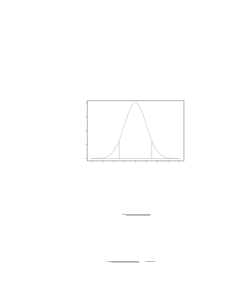
164
CHAPTER 8. INFERENCE
> 2*pnorm(-abs(z))
or by consulting a table. An illustration of the normal probability of interest
is sketched in Figure 8.1.
z
f(z)
-4
-3
-2
-1
0
1
2
3
4
0.0
0.1
0.2
0.3
0.4
Figure 8.1: P (
|Z| ≥ |z| = 1.5)
An important example of Case 1 occurs when X
i
∼ Bernoulli(µ). In this
case, σ
2
= Var X
i
= µ(1
− µ); hence, under the null hypothesis that µ = µ
0
,
σ
2
= µ
0
(1
− µ
0
) and
z =
¯
x
n
− µ
0
p
µ
0
(1
− µ
0
)/n
.
Example 1
To test H
0
: µ = .5 versus H
1
: µ
6= .5 at significance level
α = .05, we perform n = 2500 trials and observe 1200 successes. Should H
0
be rejected?
The observed proportion of successes is ¯
x
n
= 1200/2500 = .48, so the
value of the test statistic is
z =
.48
− .50
p
.5(1
− .5)/2500
=
−.02
.5/50
=
−2

8.4. TESTING HYPOTHESES ABOUT A POPULATION MEAN
165
and the significance probability is
P
.
= 2Φ(
−2)
.
= .0456 < .05 = α.
Because P
≤ α, we reject H
0
.
Case 2: The population variance is unknown.
Because σ
2
is unknown, we must estimate it from the sample. We will use
the estimator introduced in Section 8.2,
S
2
n
=
1
n
− 1
n
X
i=1
¡
X
i
− ¯
X
n
¢
2
,
and define
T
n
=
¯
X
n
− µ
0
S
n
/
√
n
.
Because S
2
n
is a consistent estimator of σ
2
, i.e. S
2
n
P
→ σ
2
, it follows from
Theorem 6.3 that
lim
n→∞
P (T
n
≤ z) = Φ(z).
Just as we could use a normal approximation to compute probabilities
involving Z
n
, so can we use a normal approximation to compute probabili-
ties involving T
n
. The fact that we must estimate σ
2
slightly degrades the
quality of the approximation; however, because n is large, we should observe
an accurate estimate of σ
2
and the approximation should not suffer much.
Accordingly, we proceed as in Case 1, using
t =
¯
x
n
− µ
0
s
n
/
√
n
instead of z.
Example 2
To test H
0
: µ = 1 versus H
1
: µ
6= 1 at significance level
α = .05, we collect n = 2500 observations, observing ¯
x
n
= 1.1 and s
n
= 2.
Should H
0
be rejected?
The value of the test statistic is
t =
1.1
− 1.0
2/50
= 2.5
and the significance probability is
P
.
= 2Φ(
−2.5)
.
= .0124 < .05 = α.
Because P
≤ α, we reject H
0
.

166
CHAPTER 8. INFERENCE
One-Sided Hypotheses
In Section 8.3 we suggested that, if Robin is not interested in whether or
not penny-spinning is fair but rather in whether or not it favors her brother,
then appropriate hypotheses would be p < .5 (penny-spinning favors Arlen)
and p
≥ .5 (penny-spinning does not favor Arlen). These are examples of
one-sided (as opposed to two-sided) hypotheses.
More generally, we will consider two canonical cases:
H
0
: µ
≤ µ
0
versus H
1
: µ > µ
0
H
0
: µ
≥ µ
0
versus H
1
: µ < µ
0
Notice that the possibility of equality, µ = µ
0
, belongs to the null hypothesis
in both cases. This is a technical necessity that arises because we compute
significance probabilities using the µ in H
0
that is nearest H
1
. For such a
µ to exist, the boundary between H
0
and H
1
must belong to H
0
. We will
return to this necessity later in this section.
Instead of memorizing different formulas for different situations, we will
endeavor to understand which values of our test statistic tend to undermine
the null hypothesis in question. Such reasoning can be used on a case-by-
case basis to determine the relevant significance probability. In so doing,
sketching crude pictures can be quite helpful!
Consider testing each of the following:
(a) H
0
: µ = µ
0
versus H
1
: µ
6= µ
0
(b) H
0
: µ
≤ µ
0
versus H
1
: µ > µ
0
(c) H
0
: µ
≥ µ
0
versus H
1
: µ < µ
0
Qualitatively, we will be inclined to reject the null hypothesis if
(a) We observe ¯
x
n
¿ µ
0
or ¯
x
n
À µ
0
, i.e. if we observe
|¯x
n
− µ
0
| À 0.
This is equivalent to observing
|t| À 0, so the significance probability
is
P
a
= P
µ
0
(
|T
n
| ≥ |t|) .
(b) We observe ¯
x
n
À µ
0
, i.e. if we observe ¯
x
n
− µ
0
À 0.
This is equivalent to observing t
À 0, so the significance probability is
P
b
= P
µ
0
(T
n
≥ t) .
(c) We observe ¯
x
n
¿ µ
0
, i.e. if we observe ¯
x
n
− µ
0
¿ 0.
This is equivalent to observing t
¿ 0, so the significance probability is
P
c
= P
µ
0
(T
n
≤ t) .

8.4. TESTING HYPOTHESES ABOUT A POPULATION MEAN
167
Example 2 (continued)
Applying the above reasoning to t = 2.5, we
obtain the significance probabilities sketched in Figure 8.2. Notice that P
b
=
P
a
/2 and that P
b
+ P
c
= 1. The probability P
b
is quite small, so we reject
H
0
: µ
≤ 1. This makes sense, because we observed ¯x
n
= 1.1 > 1.0 = µ
0
.
It is therefore obvious that the sample contains some evidence that µ > 1
and the statistical test reveals that the strength of this evidence is fairly
compelling.
(a)
-4
-3
-2
-1
0
1
2
3
4
0.0
0.1
0.2
0.3
0.4
(b)
-4
-3
-2
-1
0
1
2
3
4
0.0
0.1
0.2
0.3
0.4
(c)
-4
-3
-2
-1
0
1
2
3
4
0.0
0.1
0.2
0.3
0.4
Figure 8.2: Significance Probabilities for Example 2
In contrast, the probability of P
c
is quite large and so we decline to reject
H
0
: µ
≥ 1. This also makes sense, because the sample contains no evidence
that µ < 1. In such instances, performing a statistical test only confirms that
which is transparent from comparing the sample and hypothesized means.
Example 3
A group of concerned parents wants speed humps installed
in front of a local elementary school, but the city traffic office is reluctant
to allocate funds for this purpose. Both parties agree that humps should be
installed if the average speed of all motorists who pass the school while it is
in session exceeds the posted speed limit of 15 miles per hour (mph). Let µ
denote the average speed of the motorists in question. A random sample of

168
CHAPTER 8. INFERENCE
n = 150 of these motorists was observed to have a sample mean of ¯
x = 15.3
mph with a sample standard deviation of s = 2.5 mph.
(a) State null and alternative hypotheses that are appropriate from the
parents’ perspective.
(b) State null and alternative hypotheses that are appropriate from the city
traffic office’s perspective.
(c) Compute the value of an appropriate test statistic.
(d) Adopting the parents’ perspective and assuming that they are willing to
risk a 1% chance of committing a Type I error, what action should be
taken? Why?
(e) Adopting the city traffic office’s perspective and assuming that they are
willing to risk a 10% chance of committing a Type I error, what action
should be taken? Why?
Solution
(a) Absent compelling evidence, the parents want to install the speed
humps that they believe will protect their children. Thus, the null
hypothesis to which the parents will default is H
0
: µ
≥ 15. The par-
ents require compelling evidence that speed humps are unnecessary, so
their alternative hypothesis is H
1
: µ < 15.
(b) Absent compelling evidence, the city traffic office wants to avoid spend-
ing taxpayer dollars that might fund other public works. Thus, the null
hypothesis to which the traffic office will default is H
0
: µ
≤ 15. The
traffic office requires compelling evidence that speed humps are neces-
sary, so its alternative hypothesis is H
1
: µ > 15.
(c) Because the population variance is unknown, the appropriate test
statistic is
t =
¯
x
− µ
0
s/
√
n
=
15.3
− 15
2.5/
√
150
.
= 1.47.
(d) We would reject the null hypothesis in (a) if ¯
x is sufficiently smaller
than µ
0
= 15. Since ¯
x = 15.3 > 15, there is no evidence against
H
0
: µ
≥ 15. The null hypothesis is retained and speed humps are
installed.

8.4. TESTING HYPOTHESES ABOUT A POPULATION MEAN
169
(e) We would reject the null hypothesis in (b) if ¯
x is sufficiently larger
than µ
0
= 15, i.e. for sufficiently large positive values of t. Hence, the
significance probability is
P = P (T
n
≥ t)
.
= P (Z
≥ 1.47) = 1 − Φ(1.47)
.
= .071 < .10 = α.
Because P
≤ α, the traffic office should reject H
0
: µ
≤ 15 and install
speed humps.
Statistical Significance and Material Significance
The significance probability is the probability that a coincidence at least as
extraordinary as the phenomenon observed can be produced by chance. The
smaller the significance probability, the more confidently we reject the null
hypothesis. However, it is one thing to be convinced that the null hypothesis
is incorrect—it is something else to assert that the true state of nature is
very different from the state(s) specified by the null hypothesis.
Example 4
A government agency requires prospective advertisers to
provide statistical evidence that documents their claims. In order to claim
that a gasoline additive increases mileage, an advertiser must fund an inde-
pendent study in which n vehicles are tested to see how far they can drive,
first without and then with the additive. Let X
i
denote the increase in miles
per gallon (mpg with the additive minus mpg without the additive) observed
for vehicle i and let µ = EX
i
. The null hypothesis H
0
: µ
≤ 1 is tested
against the alternative hypothesis H
1
: µ > 1 and advertising is authorized
if H
0
is rejected at a significance level of α = .05.
Consider the experiences of two prospective advertisers:
1. A large corporation manufactures an additive that increases mileage
by an average of µ = 1.01 miles per gallon. The corporation funds
a large study of n = 900 vehicles in which ¯
x = 1.01 and s = 0.1 are
observed. This results in a test statistic of
t =
¯
x
− µ
0
s/
√
n
=
1.01
− 1.00
0.1/
√
900
= 3
and a significance probability of
P = P (T
n
≥ t)
.
= P (Z
≥ 3) = 1 − Φ(3)
.
= 0.00135 < 0.05 = α.
The null hypothesis is decisively rejected and advertising is authorized.

170
CHAPTER 8. INFERENCE
2. An amateur automotive mechanic invents an additive that increases
mileage by an average of µ = 1.21 miles per gallon. The mechanic
funds a small study of n = 9 vehicles in which ¯
x = 1.21 and s = .4 are
observed. This results in a test statistic of
t =
¯
x
− µ
0
s/
√
n
=
1.21
− 1.00
0.4/
√
9
= 1.575
and (assuming that the normal approximation is remains valid) a sig-
nificance probability of
P = P (T
n
≥ t)
.
= P (Z
≥ 1.575) = 1 − Φ(1.575)
.
= 0.05763 > 0.05 = α.
The null hypothesis is not rejected and advertising is not authorized.
These experiences are highly illuminating. Although the corporation’s
mean increase of µ = 1.01 mpg is much closer to the null hypothesis than the
mechanic’s mean increase of µ = 1.21 mpg, the corporation’s study resulted
in a much smaller significance probability. This occurred because of the
smaller standard deviation and larger sample size in the corporation’s study.
As a result, the government could be more confident that the corporation’s
product had a mean increase of more than 1.0 mpg than they could be that
the mechanic’s product had a mean increase of more than 1.0 mpg.
The preceding example illustrates that a small significance probability
does not imply a large physical effect and that a large physical effect does
not imply a small significance probability. To avoid confusing these two con-
cepts, statisticians distinguish between statistical significance and material
significance (importance). To properly interpret the results of hypothesis
testing, it is essential that one remember:
Statistical significance is not the same as material significance.
8.5
Set Estimation
Hypothesis testing is concerned with situations that demand a binary deci-
sion, e.g. whether or not to install speed humps in front of an elementary
school. The relevance of hypothesis testing in situations that do not demand
a binary decision is somewhat less clear. For example, many statisticians
feel that the scientific community overuses hypothesis testing and that other

8.5. SET ESTIMATION
171
types of statistical inference are often more appropriate. As we have dis-
cussed, a typical application of hypothesis testing in science partitions the
states of nature into two sets, one that corresponds to a theory and one
that corresponds to chance. Usually the theory encompasses a great many
possible states of nature and the mere conclusion that the theory is true
only begs the question of which states of nature are actually plausible. Fur-
thermore, it is a rather fanciful conceit to imagine that a single scientific
article should attempt to decide whether a theory is or is not true. A more
sensible enterprise for the authors to undertake is simply to set forth the
evidence that they have discovered and allow evidence to accumulate until
the scientific community reaches a consensus. One way to accomplish this is
for each article to identify what its authors consider a set of plausible values
for the population quantity in question.
To construct a set of plausible values of µ, we imagine testing H
0
: µ = µ
0
versus H
1
: µ
6= µ
0
for every µ
0
∈ (−∞, ∞) and eliminating those µ
0
for
which H
0
: µ = µ
0
is rejected. To see where this leads, let us examine our
decision criterion in the case that σ is known: we reject H
0
: µ = µ
0
if and
only if
P = P
µ
0
¡¯¯
¯
X
n
− µ
0
¯
¯
≥ |¯x
n
− µ
0
|
¢
.
= 2Φ (
− |z
n
|) ≤ α,
(8.4)
where z
n
= (¯
x
n
− µ
0
)/(σ/
√
n). Using the symmetry of the normal distribu-
tion, we can rewrite condition (8.4) as
α/2
≥ Φ (− |z
n
|) = P (Z < − |z
n
|) = P (Z > |z
n
|) ,
which in turn is equivalent to the condition
Φ (
|z
n
|) = P (Z < |z
n
|) = 1 − P (Z > |z
n
|) ≥ 1 − α/2,
(8.5)
where Z
∼ Normal(0, 1).
Now let q denote the 1
− α/2 quantile of Normal(0, 1), so that
Φ(q) = 1
− α/2.
Then condition (8.5) obtains if and only if
|z
n
| ≥ q. We express this by
saying that q is the critical value of the test statistic
|z
n
|. For example,
suppose that α = .05, so that 1
− α/2 = .975. Then the critical value is
computed in S-Plus as follows:
> qnorm(.975)
[1] 1.959964

172
CHAPTER 8. INFERENCE
Given a significance level α and the corresponding q, we have determined
that q is the critical value of
|z
n
| for testing H
0
: µ = µ
0
versus H
1
: µ
6= µ
0
at significance level α. Thus, we reject H
0
: µ = µ
0
if and only if (iff)
¯
¯
¯
¯
¯
x
n
− µ
0
σ/
√
n
¯
¯
¯
¯
=
|z
n
| ≥ q
iff
|¯x
n
− µ
0
| ≥ qσ/
√
n
iff
µ
0
6∈
¡
¯
x
n
− qσ/
√
n, ¯
x
n
+ qσ/
√
n
¢
.
Thus, the desired set of plausible values is the interval
µ
¯
x
n
− q
σ
√
n
, ¯
x
n
+ q
σ
√
n
.
(8.6)
If σ is unknown, then the argument is identical except that we estimate σ
2
as
s
2
n
=
1
n
− 1
n
X
i=1
(x
i
− ¯x
n
)
2
,
obtaining as the set of plausible values the interval
µ
¯
x
n
− q
s
n
√
n
, ¯
x
n
+ q
s
n
√
n
.
(8.7)
Example 2 (continued)
A random sample of n = 2500 observations
is drawn from a population with unknown mean µ and unknown variance
σ
2
, resulting in ¯
x
n
= 1 and s
n
= 2. Using a significance level of α = .05,
determine a set of plausible values of µ.
First, because α = .05 is the significance level, q
.
= 1.96 is the critical
value. From (8.7), an interval of plausible values is
1.1
± 1.96 · 2/
√
2500 = (1.0216, 1.1784).
Notice that 1
6∈ (1.0216, 1.1784), meaning that (as we discovered in Section
8.4) we would reject H
0
: µ = 1 at significance level α = .05.
Now consider the random interval I, defined in Case 1 (population vari-
ance known) by
I =
µ
¯
X
n
− q
σ
√
n
, ¯
X
n
− q
σ
√
n

8.5. SET ESTIMATION
173
and in Case 2 (population variance unknown) by
I =
µ
¯
X
n
− q
S
n
√
n
, ¯
X
n
− q
S
n
√
n
.
The probability that this random interval covers the real number µ
0
is
P
µ
(I
⊃ µ
0
) = 1
− P
µ
(µ
0
6∈ I) = 1 − P
µ
(reject H
0
: µ = µ
0
) .
If µ = µ
0
, then the probability of coverage is
1
− P
µ
0
(reject H
0
: µ = µ
0
) = 1
− P
µ
0
(Type I error)
≥ 1 − α.
Thus, the probability that I covers the true value of the population mean is
at least 1
− α, which we express by saying that I is a (1 − α)-level confidence
interval for µ. The level of confidence, 1
− α, is also called the confidence
coefficient.
We emphasize that the confidence interval I is random and the popu-
lation mean µ is fixed, albeit unknown. Each time that the experiment in
question is performed, a random sample is observed and an interval is con-
structed from it. As the sample varies, so does the interval. Any one such
interval, constructed from a single sample, either does or does not contain
the population mean. However, if this procedure is repeated a great many
times, then the proportion of such intervals that contain µ will be at least
1
− α. Actually observing one sample and constructing one interval from
it amounts to randomly selecting one of the many intervals that might or
might not contain µ. Because most (at least 1
−α) of the intervals do, we can
be “confident” that the interval that was actually constructed does contain
the unknown population mean.
Sample Size
Confidence intervals are often used to determine sample sizes for future ex-
periments. Typically, the researcher specifies a desired confidence level, 1
−α,
and a desired interval length, L. After determining the appropriate critical
value, q, one equates L with 2qσ/
√
n and solves for n, obtaining
n = (2qσ/L)
2
.
(8.8)
Of course, this formula presupposes knowledge of the population variance.
In practice, it is usually necessary to replace σ with an estimate—which may

174
CHAPTER 8. INFERENCE
be easier said than done if the experiment has not yet been performed. This
is one reason to perform a pilot study: to obtain a preliminary estimate of
the population variance and use it to design a better study.
Several useful relations can be deduced from equation (8.8):
1. Higher levels of confidence (1
− α) correspond to larger critical values
(q), which result in larger sample sizes (n).
2. Smaller interval lengths (L) result in larger sample sizes (n).
3. Larger variances (σ
2
) result in larger sample sizes (n).
In summary, if a researcher desires high confidence that the true mean of a
highly variable population is covered by a small interval, then s/he should
plan on collecting a great deal of data!
Example 4 (continued)
A rival corporation purchases the rights to
the amateur mechanic’s additive. How large a study is required to determine
this additive’s mean increase in mileage to within 0.05 mpg with a confidence
coefficient of 1
− α = 0.99?
The desired interval length is L = 2
· 0.05 = 0.1 and the critical value
that corresponds to α = 0.01 is computed in S-Plus as follows:
> qnorm(1-.01/2)
[1] 2.575829
From the mechanic’s small pilot study, we estimate σ to be s = 0.4. Then
n = (2
· 2.575829 · 0.4/0.1)
2
.
= 424.6,
so the desired study will require n = 425 vehicles.
1-Sided Confidence Intervals
The set of µ
0
for which we would accept the null hypothesis H
0
: µ = µ
0
when tested against the two-sided alternative hypothesis H
1
: µ
6= µ
0
is a tra-
ditional, 2-sided confidence interval. In situations where 1-sided alternatives
are appropriate, we can construct corresponding 1-sided confidence intervals
by determining the set of µ
0
for which the appropriate null hypothesis would
be accepted.

8.6. EXERCISES
175
Example 4 (continued)
The government test has a significance level
of α = 0.05. It rejects the null hypothesis H
0
: µ
≤ µ
0
if and only if (iff)
P = P (Z
≥ t) ≤ 0.05
iff
P (Z < t)
≥ 0.95
iff
t
≥ qnorm(0.95)
.
= 1.645.
Equivalently, the null hypothesis H
0
: µ
≤ µ
0
is accepted if and only if
t =
¯
x
− µ
0
s/
√
n
< 1.645
iff
¯
x < µ
0
+ 1.645
·
s
√
n
iff
µ
0
> ¯
x
− 1.645 ·
s
√
n
.
1. In the case of the large corporation, the null hypothesis H
0
: µ
≤ µ
0
is
accepted if and only if
µ
0
> 1.01
− 1.645 ·
0.1
√
900
.
= 1.0045,
so the 1-sided confidence interval with confidence coefficient 1
− α =
0.95 is (1.0045,
∞).
2. In the case of the amateur mechanic, the null hypothesis H
0
: µ
≤ µ
0
is accepted if and only if
µ
0
> 1.21
− 1.645 ·
0.4
√
9
.
= 0.9967,
so the 1-sided confidence interval with confidence coefficient 1
− α =
0.95 is (0.9967,
∞).
8.6
Exercises
1. It is thought that human influenza viruses originate in birds. It is
quite possible that, several years ago, a human influenza pandemic was
averted by slaughtering 1.5 million chickens brought to market in Hong
Kong. Because it is impossible to test each chicken individually, such
decisions are based on samples. Suppose that a boy has already died of

176
CHAPTER 8. INFERENCE
a bird flu virus apparently contracted from a chicken. Several diseased
chickens have already been identified. The health officials would prefer
to err on the side of caution and destroy all chickens that might be
infected; the farmers do not want this to happen unless it is absolutely
necessary. Suppose that both the farmers and the health officals agree
that all chickens should be destroyed if more than 2 percent of them are
diseased. A random sample of n = 1000 chickens reveals 40 diseased
chickens.
(a) Let X
i
= 1 if chicken i is diseased and X
i
= 0 if it is not. Assume
that X
1
, . . . , X
n
∼ P . To what family of probability distributions
does P belong? What population parameter indexes this family?
Use this parameter to state formulas for µ = EX
i
and σ
2
=
Var X
i
.
(b) State appropriate null and alternative hypotheses from the per-
spective of the health officials.
(c) State appropriate null and alternative hypotheses from the per-
spective of the farmers.
(d) Use the value of µ
0
in the above hypotheses to compute the value
of σ
2
under H
0
. Then compute the value of the test statistic z.
(e) Adopting the health officials’ perspective, and assuming that they
are willing to risk a 0.1% chance of committing a Type I error,
what action should be taken? Why?
(f) Adopting the farmers’ perspective, and assuming that they are
willing to risk a 10% chance of committing a Type I error, what
action should be taken? Why?
2. A company that manufactures light bulbs has advertised that its 75-
watt bulbs burn an average of 800 hours before failing. In reaction
to the company’s advertising campaign, several dissatisfied customers
have complained to a consumer watchdog organization that they be-
lieve the company’s claim to be exaggerated. The consumer organi-
zation must decide whether or not to allocate some of its financial
resources to countering the company’s advertising campaign. So that
it can make an informed decision, it begins by purchasing and testing
100 of the disputed light bulbs. In this experiment, the 100 light bulbs
burned an average of ¯
x = 745.1 hours before failing, with a sample
standard deviation of s = 238.0 hours. Formulate null and alterna-
tive hypotheses that are appropriate for this situation. Calculate a

8.6. EXERCISES
177
significance probability. Do these results warrant rejecting the null
hypothesis at a significance level of α = 0.05?
3. To study the effects of Alzheimer’s disease (AD) on cognition, a scien-
tist administers two batteries of neuropsychological tasks to 60 mildly
demented AD patients. One battery is administered in the morning,
the other in the afternoon. Each battery includes a task in which
discourse is elicited by showing the patient a picture and asking the
patient to describe it. The quality of the discourse is measured by
counting the number of “information units” conveyed by the patient.
The scientist wonders if asking a patient to describe Picture A in the
morning is equivalent to asking the same patient to describe Picture B
in the afternoon, after having described Picture A several hours ear-
lier. To investigate, she computes the number of information units for
Picture A minus the number of information units for Picture B for
each patient. She finds an average difference of ¯
x =
−0.1833, with a
sample standard deviation of s = 5.18633. Formulate null and alter-
native hypotheses that are appropriate for this situation. Calculate
a significance probability. Do these results warrant rejecting the null
hypothesis at a significance level of α = 0.05?
4. The USGS decides to use a laser altimeter to measure the height µ
of Mt. Wrightson, the highest point in Pima County, Arizona. It is
known that measurements made by the laser altimeter have an ex-
pected value equal to µ and a standard deviation of 1 meter. How
many measurements should be made if the USGS wants to construct a
0.90-level confidence interval for µ that has a length of 20 centimeters?
5. Professor Johnson is interested in the probability that a certain type
of randomly generated matrix has a positive determinant. His student
attempts to calculate the probability exactly, but runs into difficulty
because the problem requires her to evaluate an integral in 9 dimen-
sions. Professor Johnson therefore decides to obtain an approximate
probability by simulation, i.e. by randomly generating some matrices
and observing the proportion that have positive determinants. His pre-
liminary investigation reveals that the probability is roughly .05. At
this point, Professor Park decides to undertake a more comprehensive
simulation experiment that will, with .95-level confidence, correctly
determine the probability of interest to five decimal places. How many
random matrices should he generate to achieve the desired accuracy?

178
CHAPTER 8. INFERENCE

Chapter 9
1-Sample Location Problems
Measures of centrality are sometimes called location parameters. The title
of this chapter indicates an interest in a location parameter of a single popu-
lation. More specifically, we assume that X
1
, . . . , X
n
∼ P are independently
and identically distributed, we observe a random sample ~x = (x
1
, . . . , x
n
),
and we attempt to draw an inference about a location parameter of P . Be-
cause it is not always easy to identify the relevant population in a particular
experiment, we begin with some examples. For the sake of specificity, assume
that the location parameter of interest is the population median.
Example 1:
A machine is supposed to produce ball bearings that are 1
millimeter in diameter. To determine if the machine was correctly calibrated,
a sample of ball bearings is drawn and the diameter of each ball bearing is
measured. For this experiment:
• An experimental unit is a ball bearing.
• One measurement (diameter) is taken on each experimental unit.
• Let X
i
denote the diameter of ball bearing i.
Notice that we are distinguishing between experimental units, the objects
being measured (ball bearings), and units of measurement (e.g. millimeters).
Example 2:
A drug is supposed to lower blood pressure. To determine
if it does, a sample of hypertensive patients are administered the drug for
two months. Each person’s blood pressure is measured before and after the
two month period. For this experiment:
179

180
CHAPTER 9. 1-SAMPLE LOCATION PROBLEMS
• An experimental unit is a hypertensive patient.
• Two measurements (blood pressure before and after treatment) are
taken on each experimental unit.
• Let B
i
and A
i
denote the blood pressures of patient i before and after
treatment.
• Let X
i
= B
i
− A
i
, the decrease in blood pressure for patient i.
Example 3:
A graduate student investigated the effect of Parkinson’s
disease (PD) on speech breathing. She recruited 15 PD patients to partici-
pate in her study. She also recruited 15 normal control (NC) subjects. Each
NC subject was carefully matched to one PD patient with respect to sex,
age, height, and weight. The lung volume of each study participant was
measured. For this experiment:
• An experimental unit was a matched PD-NC pair.
• Two measurements (PD and NC lung volume) were taken on each
experimental unit.
• Let D
i
and C
i
denote the PD and NC lung volumes of pair i.
• Let X
i
= log(D
i
/C
i
) = log D
i
− log C
i
, the logarithm of the PD pro-
portion of NC lung volume.
This chapter is subdivided into sections according to distributional as-
sumptions about the X
i
:
9.1 If the data are assumed to be normally distributed, then we will be
interested in inferences about the population’s center of symmetry,
which we will identify as the population mean.
9.3 If the data are only assumed to be symmetrically distributed, then we
will also be interested in inferences about the population’s center of
symmetry, but we will identify it as the population median.
9.2 If the data are only assumed to be continuously distributed, then we
will be interested in inferences about the population median.
Each section is subdivided into subsections, according to the type of inference
(point estimation, hypothesis, set estimation) at issue.

9.1. THE NORMAL 1-SAMPLE LOCATION PROBLEM
181
9.1
The Normal
1-Sample Location Problem
In this section we assume that X
1
, . . . , X
n
∼ Normal(µ, σ
2
). As necessary,
we will distinguish between cases in which σ is known and cases in which σ
is unknown.
9.1.1
Point Estimation
Because normal distributions are symmetric, the location parameter µ is the
center of symmetry and therefore both the population mean and the popu-
lation median. Hence, there are (at least) two natural estimators of µ, the
sample mean ¯
X
n
and the sample median q
2
( ˆ
P
n
). Both are consistent, unbi-
ased estimators of µ. We will compare them by considering their asymptotic
relative efficiency (ARE). A rigorous definition of ARE is beyond the scope
of this book, but the concept is easily interpreted.
If the true distribution is P = N (µ, σ
2
), then the ARE of the sample
median to the sample mean for estimating µ is
e(P ) =
2
π
.
= 0.64.
This statement has the following interpretation: for large samples, using the
sample median to estimate a normal population mean is equivalent to ran-
domly discarding approximately 36% of the observations and calculating the
sample mean of the remaining 64%. Thus, the sample mean is substantially
more efficient than is the sample median at extracting location information
from a normal sample.
In fact, if P = N (µ, σ
2
), then the ARE of any estimator of µ to the
sample mean is
≤ 1. This is sometimes expressed by saying that the sample
mean is asymptotically efficient for estimating a normal mean. The sample
mean also enjoys a number of other optimal properties in this case. The
sample mean is unquestionably the preferred estimator for the normal 1-
sample location problem.
9.1.2
Hypothesis Testing
If σ is known, then the possible distributions of X
i
are
n
Normal(µ, σ
2
) :
−∞ < µ < ∞
o
.

182
CHAPTER 9. 1-SAMPLE LOCATION PROBLEMS
If σ is unknown, then the possible distributions of X
i
are
n
Normal(µ, σ
2
) :
−∞ < µ < ∞, σ > 0
o
.
We partition the possible distributions into two subsets, the null and
alternative hypotheses. For example, if σ is known then we might specify
H
0
=
n
Normal(0, σ
2
)
o
and H
1
=
n
Normal(µ, σ
2
) : µ
6= 0
o
,
which we would typically abbreviate as H
0
: µ = 0 and H
1
: µ
6= 0. Analo-
gously, if σ is unknown then we might specify
H
0
=
n
Normal(0, σ
2
) : σ > 0
o
and
H
1
=
n
Normal(µ, σ
2
) : µ
6= 0, σ > 0
o
,
which we would also abbreviate as H
0
: µ = 0 and H
1
: µ
6= 0.
More generally, for any real number µ
0
we might specify
H
0
=
n
Normal(µ
0
, σ
2
)
o
and H
1
=
n
Normal(µ, σ
2
) : µ
6= µ
0
o
if σ is known, or
H
0
=
n
Normal(µ
0
, σ
2
) : σ > 0
o
and
H
1
=
n
Normal(µ, σ
2
) : µ
6= µ
0
, σ > 0
o
if σ in unknown. In both cases, we would typically abbreviate these hy-
potheses as H
0
: µ = µ
0
and H
1
: µ
6= µ
0
.
The preceding examples involve two-sided alternative hypotheses. Of
course, as in Section 8.4, we might also specify one-sided hypotheses. How-
ever, the material in the present section is so similar to the material in
Section 8.4 that we will only discuss two-sided hypotheses.
The intuition that underlies testing H
0
: µ = µ
0
versus H
1
: µ
6= µ
0
was
discussed in Section 8.4:
• If H
0
is true, then we would expect the sample mean to be close to the
population mean µ
0
.
• Hence, if ¯
X
n
= ¯
x
n
is observed far from µ
n
, then we are inclined to
reject H
0
.

9.1. THE NORMAL 1-SAMPLE LOCATION PROBLEM
183
To make this reasoning precise, we reject H
0
if and only if the significance
probability
P = P
µ
0
¡¯¯
¯
X
n
− µ
0
¯
¯
≥ |¯x
n
− µ
0
|
¢
≤ α.
(9.1)
The first equation in (9.1) is a formula for a significance probability.
Notice that this formula is identical to equation (8.2). The one difference
between the material in Section 8.4 and the present material lies in how one
computes P . For emphasis, we recall the following:
1. The hypothesized mean µ
0
is a fixed number specified by the null
hypothesis.
2. The estimated mean, ¯
x
n
, is a fixed number computed from the sample.
Therefore, so is
|¯x
n
− µ
0
|, the difference between the estimated mean
and the hypothesized mean.
3. The estimator, ¯
X
n
, is a random variable.
4. The subscript in P
µ
0
reminds us to compute the probability under
H
0
: µ = µ
0
.
5. The significance level α is a fixed number specified by the researcher,
preferably before the experiment was performed.
To apply (9.1), we must compute P . In Section 8.4, we overcame that
technical difficulty by appealing to the Central Limit Theorem. This allowed
us to approximate P even when we did not know the distribution of the
X
i
, but only for reasonably large sample sizes. However, if we know that
X
1
, . . . , X
n
are normally distributed, then it turns out that we can calculate
P exactly, even when n is small.
Case 1: The Population Variance is Known
Under the null hypothesis that µ = µ
0
, X
1
, . . . , X
n
∼ Normal(µ
0
, σ
2
) and
¯
X
n
∼ Normal
³
µ
0
, σ
2
´
.
This is the exact distribution of ¯
X
n
, not an asymptotic approximation. We
convert ¯
X
n
to standard units, obtaining
Z =
¯
X
n
− µ
0
σ/
√
n
∼ Normal
³
µ
0
, σ
2
´
.
(9.2)

184
CHAPTER 9. 1-SAMPLE LOCATION PROBLEMS
The observed value of Z is
z =
¯
x
n
− µ
0
σ/
√
n
.
The significance probability is
P
= P
µ
0
¡¯¯
¯
X
n
− µ
0
¯
¯
≥ |¯x
n
− µ
0
|
¢
= P
µ
0
ï¯
¯
¯
¯
¯
X
n
− µ
0
σ/
√
n
¯
¯
¯
¯
¯
≥
¯
¯
¯
¯
¯
x
n
− µ
0
σ/
√
n
¯
¯
¯
¯
!
= P (
|Z| ≥ |z|)
= 2P (Z
≥ |z|) .
In this case, the test that rejects H
0
if and only if P
≤ α is sometimes called
the 1-sample z-test. The random variable Z is the test statistic.
Before considering the case of an unknown population variance, we re-
mark that it is possible to derive point estimators from hypothesis tests. For
testing H
0
: µ = µ
0
vs. H
1
: µ
6= µ
0
, the test statistics are
Z(µ
0
) =
¯
X
n
− µ
0
σ/
√
n
.
If we observe ¯
X
n
= ¯
x
n
, then what value of µ
0
minimizes
|z(µ
0
)
|? Clearly,
the answer is µ
0
= ¯
x
n
. Thus, our preferred point estimate of µ is the µ
0
for
which it is most difficult to reject H
0
: µ = µ
0
. This type of reasoning will
be extremely useful for analyzing situations in which we know how to test
but don’t know how to estimate.
Case 2: The Population Variance is Unknown
Statement (9.2) remains true if σ is unknown, but it is no longer possible
to compute z. Therefore, we require a different test statistic for this case.
A natural approach is to modify Z by replacing the unknown σ with an
estimator of it. Toward that end, we introduce the test statistic
T
n
=
¯
X
n
− µ
0
S
n
/
√
n
,
where S
2
n
is the unbiased estimator of the population variance defined by
equation (8.1). Because T
n
and Z are different random variables, they have
different probability distributions and our first order of business is to deter-
mine the distribution of T
n
.
We begin by stating a useful fact:

9.1. THE NORMAL 1-SAMPLE LOCATION PROBLEM
185
Theorem 9.1 If X
1
, . . . , X
n
∼ Normal(µ, σ
2
), then
(n
− 1)S
2
n
σ
2
=
n
X
i=1
¡
X
i
− ¯
X
n
¢
2
/σ
2
∼ χ
2
(n
− 1).
The χ
2
(chi-squared) distribution was described in Section 4.5 and Theorem
9.1 is closely related to Theorem 4.3.
Next we write
T
n
=
¯
X
n
− µ
0
S
n
/
√
n
=
¯
X
n
− µ
0
σ/
√
n
·
σ/
√
n
S
n
/
√
n
= Z
·
σ
S
n
= Z/
q
S
2
n
/σ
2
= Z/
q
[(n
− 1)S
2
n
/σ
2
] /(n
− 1).
Using Theorem 9.1, we see that T
n
can be written in the form
T
n
=
Z
p
Y /ν
,
where Z
∼ Normal(0, 1) and Y ∼ χ
2
(ν). If Z and Y are independent random
variables, then it follows from Definition 4.7 that T
n
∼ t(n − 1).
Both Z and Y = (n
− 1)S
2
n
/σ
2
depend on X
1
, . . . , X
n
, so one would be
inclined to think that Z and Y are dependent. This is usually the case,
but it turns out that they are independent if X
1
, . . . , X
n
∼ Normal(µ, σ
2
).
This is another remarkable property of normal distributions, usually stated
as follows:
Theorem 9.2 If X
1
, . . . , X
n
∼ Normal(µ, σ
2
), then ¯
X
n
and S
2
n
are inde-
pendent random variables.
The result that interests us can then be summarized as follows:
Corollary 9.1 If X
1
, . . . , X
n
∼ Normal(µ
0
, σ
2
), then
T
n
=
¯
X
n
− µ
0
S
n
/
√
n
∼ t(n − 1).
Now let
t
n
=
¯
x
n
− µ
0
s
n
/
√
n
,

186
CHAPTER 9. 1-SAMPLE LOCATION PROBLEMS
the observed value of the test statistic T
n
. The significance probability is
P = P (
|T
n
| ≥ |t
n
|) = 2P (T
n
≥ |t
n
|) .
In this case, the test that rejects H
0
if and only if P
≤ α is called Student’s
1-sample t-test. Because it is rarely the case that the population variance is
known when the population mean is not, Student’s 1-sample t-test is used
much more frequently than the 1-sample z-test. We will use the S-Plus
function pt to compute significance probabilities for Student’s 1-sample t-
test, as illustrated in the following examples.
Example 1
Test H
0
: µ = 0 vs. H
1
: µ
6= 0, a 2-sided alternative.
• Suppose that n = 25 and that we observe ¯x = 1 and s = 3.
• Then t = (1 − 0)/(3/
√
25)
.
= 1.67 and the 2-tailed significance proba-
bility is computed using both tails of the t(24) distribution, i.e. P =
2
∗ pt(−1.67, df = 24)
.
= 0.054.
Example 2
Test H
0
: µ
≤ 0 vs. H
1
: µ > 0, a 1-sided alternative.
• Suppose that n = 25 and that we observe ¯x = 2 and s = 5.
• Then t = (2 − 0)/(5/
√
25) = 2.00 and the 1-tailed significance prob-
ability is computed using one tail of the t(24) distribution, i.e. P =
1
− pt(2.00, df = 24)
.
= 0.028.
9.1.3
Interval Estimation
As in Section 8.5, we will derive confidence intervals from tests. We imagine
testing H
0
: µ = µ
0
versus H
1
: µ
6= µ
0
for every µ
0
∈ (−∞, ∞). The µ
0
for
which H
0
: µ = µ
0
is rejected are implausible values of µ; the µ
0
for which
H
0
: µ = µ
0
is accepted constitute the confidence interval. To accomplish
this, we will have to derive the critical values of our tests. A significance
level of α will result in a confidence coefficient of 1
− α.
Case 1: The Population Variance is Known
If σ is known, then we reject H
0
: µ = µ
0
if and only if
P = P
µ
0
¡¯¯
¯
X
n
− µ
0
¯
¯
≥ |¯x
n
− µ
0
|
¢
= 2Φ (
− |z
n
|) ≤ α,

9.1. THE NORMAL 1-SAMPLE LOCATION PROBLEM
187
where z
n
= (¯
x
n
− µ
0
)/(σ/
√
n). By the symmetry of the normal distribution,
this condition is equivalent to the condition
1
− Φ (− |z
n
|) = P (Z > − |z
n
|) = P (Z < |z
n
|) = Φ (|z
n
|) ≥ 1 − α/2,
where Z
∼ Normal(0, 1), and therefore to the condition |z
n
| ≥ q
z
, where q
z
denotes the 1
− α/2 quantile of Normal(0, 1). The quantile q
z
is the critical
value of the two-sided 1-sample z-test. Thus, given a significance level α and
a corresponding critical value q
z
, we reject H
0
: µ = µ
0
if and only if (iff)
¯
¯
¯
¯
¯
x
n
− µ
0
σ/
√
n
¯
¯
¯
¯
=
|z
n
| ≥ q
z
iff
|¯x
n
− µ
0
| ≥ q
z
σ/
√
n
iff
µ
0
6∈
¡
¯
x
n
− q
z
σ/
√
n, ¯
x
n
+ q
z
σ/
√
n
¢
and we conclude that the desired set of plausible values is the interval
µ
¯
x
n
− q
z
σ
√
n
, ¯
x
n
+ q
z
σ
√
n
.
Notice that both the preceding derivation and the resulting confidence
interval are identical to the derivation and confidence interval in Section 8.5.
The only difference is that, because we are now assuming that X
1
, . . . , X
n
∼
Normal(µ, σ
2
) instead of relying on the Central Limit Theorem, no approx-
imation is required.
Example 3
Suppose that we desire 90% confidence about µ and σ = 3
is known. Then α = .10 and q
z
.
= 1.645. Suppose that we draw n = 25
observations and observe ¯
x
n
= 1. Then
1
± 1.645
3
√
25
= 1
± .987 = (.013, 1.987)
is a .90-level confidence interval for µ.
Case 2: The Population Variance is Unknown
If σ is unknown, then it must be estimated from the sample. The reasoning
in this case is the same, except that we rely on Student’s 1-sample t-test.
As before, we use S
2
n
to estimate σ
2
. The critical value of the 2-sided
1-sample t-test is q
t
, the 1
−α/2 quantile of a t distribution with n−1 degrees
of freedom, and the confidence interval is
µ
¯
x
n
− q
t
s
n
√
n
, ¯
x
n
+ q
t
s
n
√
n
.

188
CHAPTER 9. 1-SAMPLE LOCATION PROBLEMS
Example 4
Suppose that we desire 90% confidence about µ and σ is
unknown. Suppose that we draw n = 25 observations and observe ¯
x
n
= 1
and s = 3. Then t
q
= qt(.95, df = 24)
.
= 1.711 and
1
± 1.711 × 3/
√
25 = 1
± 1.027 = (−.027, 2.027)
is a 90% confidence interval for µ. Notice that the confidence interval is
larger when we use s = 3 instead of σ = 3.

9.2. THE GENERAL 1-SAMPLE LOCATION PROBLEM
189
9.2
The General
1-Sample Location Problem
• Assume that X
1
, . . . , X
n
∼ P .
• Since P is not assumed to be symmetric, we must decide which location
parameter is of interest. Because the population mean may not exist,
we usually are interested in inferences about the population median
M .
• We assume only that the X
i
are continuous random variables.
9.2.1
Point Estimation
• The (only) natural estimator of the population median M is the sample
median ˜
X
n
.
9.2.2
Hypothesis Testing
• As before, we initially consider testing a 2-sided alternative, H
0
: M =
M
0
vs. H
1
: M
6= M
0
.
• Under H
0
, we would expect to observe ˜
X
n
= ˜
x
n
near M
0
, i.e. approx-
imately half the data above M
0
and half the data below M
0
.
• Let p
+
= P
H
0
(X
i
> M
0
) and p
−
= P
H
0
(X
i
< M
0
). Because the X
i
are continuous, p
+
= p
−
= .5. Thus, observing if X
i
is greater or less
than M
0
is equivalent to tossing a fair coin, i.e. performing a Bernoulli
trial.
• The Sign Test is the following procedure:

190
CHAPTER 9. 1-SAMPLE LOCATION PROBLEMS
– Let x
1
, . . . , x
n
denote the observed sample. Because the X
i
are
continuous, P (X
i
= M
0
) = 0 and we ought not to observe any
x
i
= M
0
. In practice, of course, this may happen. For the mo-
ment, we assume that it has not.
– Let
S
+
= #
{X
i
> M
0
} = #{X
i
− M
0
> 0
}
be the test statistic. Under H
0
, S
+
∼ Binomial(n, .5).
– Let
p = P
H
0
µ
|S
+
−
n
2
| ≥ |s
+
−
n
2
|
be the significance probability.
– The sign test rejects H
0
: M = M
0
if and only if p
≤ α.
– For small n, we compute p using a table of binomial probabilities;
for larger n, we use the normal approximation. Both techniques
will be explained in the examples that follow.
• We now consider three strategies for dealing with the possibility that
several x
i
= M
0
. We assume that these observations represent only
a small fraction of the sample; otherwise, the assumption that the X
i
are continuous was not warranted.
– The most common practice is to simply discard the x
i
= M
0
be-
fore performing the analysis. Notice, however, that this is discard-
ing evidence that supports H
0
, thereby increasing the probability
of a Type I error, so this is a somewhat risky course of action.
– Therefore, it may be better to count half of the x
i
= M
0
as larger
than M
0
and half as smaller. If the number of these observations
is odd, then this will result in a non-integer value of the test
statistic S
+
. To compute the significance probability in this case,
we can either rely on the normal approximation, or compute two
p-values, one corresponding to S
+
+ .5 and one corresponding to
S
+
− .5.
– Perhaps the most satisfying solution is to compute all of the signif-
icance probabilities that correspond to different ways of counting
the x
i
= M
0
as larger and smaller than M
0
. Actually, it will
suffice to compute the p-value that corresponds to counting all of
the x
i
= M
0
as larger than M
0
and the p-value corresponds to

9.2. THE GENERAL 1-SAMPLE LOCATION PROBLEM
191
counting all of the x
i
= M
0
as smaller than M
0
. If both of these
p-values are less than (or equal to) the significance level α, then
clearly we will reject H
0
. If neither is, then clearly we will not.
If one is and one is not, then we will declare the evidence to be
equivocal.
• Example 2.3 from Gibbons
– Suppose that we want to test H
0
: M = 10 vs. H
1
: M
6= 10 at
significance level α = .05.
– Suppose that we observe the following sample:
9.8
10.1
9.7
9.9
10.0
10.0
9.8
9.7
9.8
9.9
– Note the presence of ties in the data, suggesting that the mea-
surements should have been made (or recorded) more precisely.
In particular, there are two instances in which x
i
= M
0
.
– If we discard the two x
i
= 10, then n = 8, s
+
= 1, and
p = P (
|S
+
− 4| ≥ |1 − 4| = 3)
= P (S
+
≤ 1 or S
+
≥ 7)
= 2P (S
+
≤ 1)
= 2
× .0352 = .0704,
from Table F in Gibbons (see handout).
– Since p = .0704 > .05 = α, we decline to reject H
0
.
• Example 2.4 from Gibbons
– Suppose that we want to test H
0
: M
≤ 625 vs. H
1
: M > 625 at
significance level α = .05.
– Suppose that we observe the following sample:
612
619
628
631
640
643
649
655
663
670
– Here, n = 10, s
+
= 8, and
p = P (S
+
≥ 8) = P (S
+
≤ 2) = .0547,
from Table F in Gibbons (see handout).
– Since p = .0547 > .05 = α, we decline to reject H
0
.

192
CHAPTER 9. 1-SAMPLE LOCATION PROBLEMS
• If n > 20, then we use the normal approximation to the binomial
distribution. Since S
+
∼ Binomial(n, .5), S
+
has expected value .5n
and standard deviation .5
√
n. The normal approximation is
P (S
+
≥ k)
.
= P
µ
Z
≥
k
− .5 − .5n
.5
√
n
,
where Z
∼ N(0, 1).
• Example 2.4 (continued):
P (S
+
≥ 8)
.
= P
µ
Z
≥
8
− .5 − 5
.5
√
10
.
= 1.58
.
= .0571.
• Notice that the sign test will produce a maximal significance proba-
bility of p = 1 when S
+
= S
−
= .5n. This means that the sign test
is least likely to reject H
0
: M = M
0
when M
0
is a median of the
sample. Thus, using the sign test for testing hypotheses about popu-
lation medians corresponds to using the sample median for estimating
population medians, just as using Student’s t-test for testing hypothe-
ses about population means corresponds to using the sample mean for
estimating population means.
• One consequence of the previous remark is that, when the population
mean and median are identical, the “Pitman efficiency” of the sign
test to Student’s t-test equals the asymptotic relative efficiency of the
sample median to the sample median. For example, using the sign test
on normal data is asymptotically equivalent to randomly discarding
36% of the observations, then using Student’s t-test on the remaining
64%.
9.2.3
Interval Estimation
• We want to construct a (1 − α)-level confidence interval for the pop-
ulation median M . We will do so by determining for which M
0
the
level-α sign test of H
0
: M = M
0
vs. H
1
: M
6= M
0
will accept H
0
.
• Suppose that we have ordered the data:
x
(1)
< x
(2)
<
· · · < x
(n−1)
< x
(n)

9.2. THE GENERAL 1-SAMPLE LOCATION PROBLEM
193
• The sign test rejects H
0
: M = M
0
if
|S
+
− .5n| is large, i.e. H
0
will
be accepted if M
0
is such that the numbers of observations above and
below M
0
are roughly equal.
• Suppose that
P (S
+
≤ k) = P (S
+
≥ n − k) = α/2.
For n
≤ 20, we can use Table F to determine pairs of (α, k) that satisfy
this equation. Notice that only certain α are possible, so that we may
not be able to exactly achieve the desired level of confidence.
• Having determined an acceptable (α, k), the sign test would accept
H
0
: M = M
0
at level α if and only if
x
(k+1)
< M
0
< x
(n−k)
;
hence, a (1
− α)-level confidence interval for M is
(x
(k+1)
, x
(n−k)
).
• Remark: Since there is no fixed M
0
when constructing a confidence
interval, we always use all of the data.
• Example 2.4 in Gibbons (continued): From Table F,
P (S
+
≤ 2) = P (S
+
≥ 8) = .0547;
hence, a (1
− 2 × .0547) = .8906-level confidence interval for M is
(628, 655).
• For n > 20, we can use the normal approximation to the binomial to
determine k.
– If we specify α in
P (S
+
≥ n − k) = P
µ
Z
≥
n
− k − .5 − .5n
.5
√
n
= z
=
α
2
,

194
CHAPTER 9. 1-SAMPLE LOCATION PROBLEMS
then
k = .5(n
− 1 − z
√
n).
– For example, α = .05 entails z = 1.96. If n = 100, then
k = .5(100
− 1 − 1.96
√
100) = 39.7
and the desired confidence interval is approximately
(x
(41)
, x
(60)
),
which is slightly liberal, or
(x
(40)
, x
(61)
),
which is slightly conservative.
9.3
The Symmetric
1-Sample Location Problem
• Assume that X
1
, . . . , X
n
∼ P .
• We assume that the X
i
are continuous random variables with symmet-
ric pdf f . Let θ denote the center of symmetry. Note, in particular,
that θ = M , the population median.
9.3.1
Hypothesis Testing
• As before, we initially consider testing a 2-sided alternative, H
0
: θ = θ
0
vs. H
1
: θ = θ
0
.
• Let D
i
= X
i
− θ
0
. Because the X
i
are continuous, P (D
i
= 0) = 0 and
P (
|D
i
| = |D
j
|) = 0 for i 6= j. Therefore, we can rank the absolute
differences as follows:
|D
i
1
| < |D
i
2
| < · · · < |D
i
n
|.
Let R
i
denote the rank of
|D
i
|.

9.3. THE SYMMETRIC 1-SAMPLE LOCATION PROBLEM
195
• The Wilcoxon Signed Rank Test is the following procedure:
– Let x
1
, . . . , x
n
denote the observed sample and let d
i
= x
i
− θ
0
.
Initially, we assume that no d
i
= 0 or
|d
i
| = |d
j
| were observed.
– We define two test statistics,
T
+
=
X
D
ik
>0
k,
the sum of the “positive ranks,” and
T
−
=
X
D
ik
<0
k,
the sum of the “negative ranks.”
– Notice that
T
+
+ T
−
=
n
X
k=1
k = n(n + 1)/2,
so that it suffices to consider only T
+
(or T
−
, whichever is more
convenient).
– By symmetry, under H
0
: θ = θ
0
we have
ET
+
= ET
−
= n(n + 1)/4.
– The Wilcoxon signed rank test rejects H
0
if and only if we observe
T
+
sufficently different from ET
+
, i.e. if and only if
p = P
H
0
(
|T
+
− n(n + 1)/4) ≥ |t
+
− n(n + 1)/4|) ≤ α.
• For n ≤ 15, we can compute the significance probability p from Table
G in Gibbons.
• Example 3.1 from Gibbons
– Suppose that we want to test H
0
: M = 10 vs. H
1
: M
6= 10 at
significance level α = .05.
– Suppose that we observe the following sample:

196
CHAPTER 9. 1-SAMPLE LOCATION PROBLEMS
x
i
d
i
r
i
9.83
-.17
7
10.09
.09
3
9.72
-.28
10
9.87
-.13
5
10.04
.04
1
9.95
-.05
2
9.82
-.18
6
9.73
-.27
9
9.79
-.21
8
9.90
-.10
4
– Then n = 10, ET
+
= 10(11)/4 = 27.5, t
+
= 3 + 1 = 4, and
p = P (
|T
+
− 27.5| ≥ |4 − 27.5| = 23.5)
= P (T
+
≤ 4 or T
+
≥ 51)
= 2P (T
+
≤ 4)
= 2
× .007 = .014,
from Table G in Gibbons (see handout).
– Since p = .014 < .05 = α, we reject H
0
.
• For n ≥ 16, we convert T
+
to standard units and use the normal
approximation:
– Under H
0
: θ = θ
0
, ET
+
= n(n + 1)/4, and
VarT
+
= n(n + 1)(2n + 1)/24.
– For n sufficiently large,
Z =
T
+
− ET
+
√
VarT
+
˙
∼N(0, 1).
– In the above example,
VarT
+
= 10(11)(21)/24 = 96.25
and
z =
t
+
− ET
+
√
VarT
+
=
4
− 27.5
√
96.5
.
=
−2.40,

9.3. THE SYMMETRIC 1-SAMPLE LOCATION PROBLEM
197
which gives an approximate significance probability of
p = 2P (Z
≤ z = −2.40)
= 2 [.5
− P (0 ≤ Z < 2.40)]
= 2(.5
− .4918)
= .0164.
• Ties. Now suppose that the |d
i
| > 0, but not necessarily distinct. If
the number of ties is small, then one can perform the test using each
possible ordering of the
|d
i
|. Otherwise:
– If several
|D
i
| are tied, then each is assigned the average of the
ranks to be assigned to that set of
|D
i
|. These ranks are called
midranks. For example, if we observe
|d
i
| = 8, 9, 10, 10, 12, then
the midranks are r
i
= 1, 2, 3.5, 3.5, 5.
– We then proceed as above using the midranks. Since Table G was
calculated on the assumption of no ties, we must use the normal
approximation. The formula for ET
+
is identical, but the formula
for VarT
+
becomes more complicated.
– Suppose that there are J distinct values of
|D
i
|. Let u
j
denote
the number of
|D
i
| equalling the jth distinct value. Then
VarT
+
=
n(n + 1)(2n + 1)
24
−
1
48
J
X
j=1
(u
3
j
− u
j
).
– Notice that, if u
j
= 1 (as typically will be the case for most of
the values), then u
3
j
− u
j
= 0.
• If any d
i
= 0, i.e. if any x
i
= θ
0
, then we can adopt any of the strategies
that we used with the sign test when we observed x
i
= M
0
.
9.3.2
Point Estimation
• We derive an estimator ˆθ of θ by determining the value of θ
0
for which
the Wilcoxon signed rank test is least inclined to reject H
0
: θ = θ
0
in
favor of H
1
: θ
6= θ
0
. Our derivation relies on a clever trick.
• Suppose that
x
(1)
<
· · · < x
(k)
< θ
0
< x
(k+1)
<
· · · < x
(n)
.

198
CHAPTER 9. 1-SAMPLE LOCATION PROBLEMS
• Notice that, if i ≤ j ≤ k, then
³
x
(i)
− θ
0
´
+
³
x
(j)
− θ
0
´
< 0.
• For j = k + 1, . . . , n,
r
j
=
rank of d
j
=
|x
(j)
− θ
0
|
=
#
{i : i ≤ j, |x
(i)
− θ
0
| ≤ |x
(j)
− θ
0
|}
=
#
{i : i ≤ j, −(x
(i)
− θ
0
)
≤ x
(j)
− θ
0
}
=
#
{i : i ≤ j, (x
(i)
− θ
0
) + (x
(j)
− θ
0
)
≥ 0}.
• Therefore,
t
+
=
r
k+1
+
· · · r
n
=
#
{i ≤ j, (x
(i)
− θ
0
) + (x
(j)
− θ
0
)
≥ 0}
=
#
{i ≤ j, (x
i
− θ
0
) + (x
j
− θ
0
)
≥ 0}
• We know that H
0
: θ = θ
0
is most difficult to reject if t
+
= ET
+
=
n(n + 1)/2. From our new representation of t
+
, this occurs when half
of the (x
i
− θ
0
) + (x
j
− θ
0
) are positive and half are negative; i.e. when
2θ
0
is the median of the pairwise sums (x
i
+ x
j
); i.e. when θ
0
is the
median of the pairwise averages (x
i
+ x
j
)/2.
• The pairwise averages (x
i
+ x
j
)/2, for 1
≤ i ≤ j ≤ n, are sometimes
called the Walsh averages. The estimator ˆ
θ of θ that corresponds to
the Wilcoxon signed rank test is the median of the Walsh averages.
• The following table reports the asymptotic relative efficiency of ˆθ to
¯
X for estimating the center of symmetry of several symmetric distri-
butions.
Family
ARE
Normal
3/π
.
= .955
Logistic
π
2
/9
.
= 1.097
Double Exponential
1.5
Uniform
1.0
σ
2
<
∞
≥ .864
9.3.3
Interval Estimation
• We construct a (1 − α)-level confidence interval for θ by including θ
0
in the interval if and only if the Wilcoxon signed rank test accepts
H
0
: θ = θ
0
vs. H
1
: θ
6= θ
0
at significance level α. As we found

9.3. THE SYMMETRIC 1-SAMPLE LOCATION PROBLEM
199
when deriving confidence intervals from the sign test, not all levels are
possible.
• From the preceding section, we know that we can represent the test
statistic T
+
as the number of Walsh averages that exceed θ
0
. Because
we reject if this number is either too large or too small, we accept
if there are sufficient numbers of Walsh averages below and above θ
0
.
Hence, the desired confidence interval must consist of those θ
0
for which
at least k
−1 Walsh averages are ≤ θ
0
and at least k
−1 Walsh averages
are
≥ θ
0
. The number k is determined by the level of confidence that
is desired.
• For example, suppose that we desire the level of confidence to be 1−α =
.90, so that α/2 = .05.
– Suppose that we observe n = 8 values:
-1
2
3
4
5
6
9
13
– The n(n + 1)/2 = 36 Walsh averages are:
-1
2
3
4
5
6
9
13
.5
2.5
3.5
4.5
5.5
7.5
11
1
3
4
5
7
9.5
1.5
3.5
4.5
6.5
9
2
4
6
8.5
(2.5)
5.5
(8)
4
7.5
4
– For n = 8 in Table G, p = P (T
+
≤ 6) = P (T
+
≥ 30) = .055.
Hence, we would reject H
0
: θ = θ
0
at α = .11 if and only if
≤ 6
Walsh averages are
≤ θ
0
or
≥ 30 Walsh averages are ≤ θ
0
.
– Hence, the .89-level confidence interval for θ should have a lower
endpoint equal to the (k = 7)th Walsh average and an upper
endpoint equal to the (n(n + 1)/2 + 1
− k = 30)th Walsh average.
By inspection, the confidence interval is [2.5, 8.0]. Notice that the
endpoints are included.
• For n ≥ 16, we can use the normal approximation to determine k. The
formula is
k = 0.5 + ET
+
− z
1−α/2
p
VarT
+
.

200
CHAPTER 9. 1-SAMPLE LOCATION PROBLEMS
9.4
A Case Study from Neuropsychology
McGlynn and Kaszniak (1991) investigated awareness of cognitive deficit in
patients suffering from Alzheimer’s disease (AD). They recruited 8 pairs of
AD patients and their spousal caregivers (CG). An examiner described a
neuropsychological task to each subject, asked the subject to predict how
both he/she and his/her spouse would perform on it, and then administered
the task. For this experiment:
• A unit of observation was a matched AD-CG pair.
• Six measurements were taken on each unit of observation:
ppp
patient prediction of patient
pscor
patient score
ppc
patient prediction of caregiver
cscor
caregiver score
cpc
caregiver prediction of caregiver
cpp
caregiver prediction of patient
• Trosset & Kaszniak (1996) proposed Comparative Predictive Accuracy
(CPA) as a measure of deficit unawareness:
CP A =
(ppp/pscor)
÷ (ppc/cscor)
(cpc/cscor)
÷ (cpp/pscor)
• Let X
i
= log(CP A
i
), the logarithm of the AD deficit unawareness
observed for pair i.

9.5. EXERCISES
201
9.5
Exercises
Problem Set A
The following data are from Darwin (1876), The Effect
of Cross- and Self-Fertilization in the Vegetable Kingdom, Second Edition,
London: John Murray. Pairs of seedlings of the same age (one produced
by cross-fertilization, the other by self-fertilization) were grown together so
that the members of each pair were reared under nearly identical conditions.
The aim was to demonstrate the greater vigour of the cross-fertilized plants.
The data are the final heights (in inches) of each plant after a fixed period
of time. Darwin consulted Francis Galton about the analysis of these data,
and they were discussed further in Ronald Fisher’s Design of Experiments.
Pair
Fertilized
Cross
Self
1
23.5
17.4
2
12.0
20.4
3
21.0
20.0
4
22.0
20.0
5
19.1
18.4
6
21.5
18.6
7
22.1
18.6
8
20.4
15.3
9
18.3
16.5
10
21.6
18.0
11
23.3
16.3
12
21.0
18.0
13
22.1
12.8
14
23.0
15.5
15
12.0
18.0
1. Show that this problem can be formulated as a 1-sample location prob-
lem. To do so, you should:
(a) Identify the experimental units and the measurement(s) taken on
each unit.
(b) Define appropriate random variables X
1
, . . . , X
n
∼ P . Remem-
ber that the statistical procedures that we will employ assume
that these random variables are independent and identically dis-
tributed.

202
CHAPTER 9. 1-SAMPLE LOCATION PROBLEMS
(c) Let θ denote the location parameter (measure of centrality) of
interest. Depending on which statistical procedure we decide to
use, either θ = EX
i
= µ or θ = q
2
(X
i
). State appropriate null
and alternative hypotheses about θ.
2. Does it seem reasonable to assume that the sample ~x = (x
1
, . . . , x
n
),
the observed values of X
1
, . . . , X
n
, were drawn from:
(a) a normal distribution? Why or why not?
(b) a symmetric distribution? Why or why not?
3. Assume that X
1
, . . . , X
n
are normally distributed and let θ = EX
i
= µ.
(a) Test the null hypothesis derived above using Student’s 1-sample
t-test. What is the significance probability? If we adopt a signif-
icance level of α = 0.05, should we reject the null hypothesis?
(b) Construct a (2-sided) confidence interval for θ with a confidence
coefficient of approximately 0.90.
4. Now we drop the assumption of normality. Assume that X
1
, . . . , X
n
are
symmetric (but not necessarily normal), continuous random variables
and let θ = q
2
(X
i
).
(a) Test the null hypothesis derived above using the Wilcoxon signed
rank test. What is the significance probability? If we adopt a
significance level of α = 0.05, should we reject the null hypothesis?
(b) Estimate θ by computing the median of the Walsh averages.
(c) Construct a (2-sided) confidence interval for θ with a confidence
coefficient of approximately 0.90.
5. Finally we drop the assumption of symmetry, assuming only that
X
1
, . . . , X
n
are continuous random variables, and let θ = q
2
(X
i
).
(a) Test the null hypothesis derived above using the sign test. What
is the significance probability? If we adopt a significance level of
α = 0.05, should we reject the null hypothesis?
(b) Estimate θ by computing the sample median.
(c) Construct a (2-sided) confidence interval for θ with a confidence
coefficient of approximately 0.90.

Chapter 10
2-Sample Location Problems
• The title of this chapter indicates an interest in comparing the location
parameters of two populations. That is, we assume that:
– X
1
, . . . , X
n
1
∼ P
1
and Y
1
, . . . , Y
n
2
∼ P
2
. Notice that we do not
assume that n
1
= n
2
.
– The X
i
and the Y
j
are continuous random variables.
– The X
i
and the Y
j
are mutually independent. In particular, there
is no natural pairing of X
1
with Y
1
, etc.
• We observe random samples x
1
, . . . , x
n
1
and y
1
, . . . , y
n
2
. From the sam-
ples, we attempt to draw an inference about the difference in location
of P
1
and P
2
. This difference, which we will denote by ∆, is called
the shift parameter. For example, we might define ∆ = µ
1
− µ
2
, where
µ
1
= EX
i
and µ
2
= EY
j
.
• Each of the structures that we encountered in 1-sample problems may
also be encountered in 2-sample problems. What distinguishes the two
are that the units of observations are drawn from one population in the
former and from two populations in the latter. The prototypical case
of the latter is that of a treatment population and a control population.
We now consider some examples.
• Example 1: A researcher investigated the effect of Alzheimer’s disease
(AD) on the ability to perform a confrontation naming task. She re-
cruited 60 mildly demented AD patients and 60 normal elderly control
subjects. The control subjects resembled the AD patients in that the
203

204
CHAPTER 10. 2-SAMPLE LOCATION PROBLEMS
two groups had comparable mean ages, years of education, and (esti-
mated) IQ scores; however, the control subjects were not individually
matched to the AD patients. Each person was administered the Boston
Naming Test. For this experiment,
– An experimental unit is a person.
– The experimental units belong to one of two populations: AD
patients or normal elderly persons.
– One measurement (BNT) is taken on each unit of observation.
– Let X
i
denote the BNT score for AD patient i. Let Y
j
denote the
BNT score for control subject j.
– Let µ
1
= EX
i
, µ
2
= EY
j
, and ∆ = µ
1
− µ
2
.
• Example 2: A drug is supposed to lower blood pressure. To determine
if it does, n
1
+n
2
hypertensive patients are recruited to participate in a
double-blind study. The patients are randomly assigned to a treatment
group of n
1
patients and a control group of n
2
patients. Each patient in
the treatment group receives the drug for two months; each patient in
the control group receives a placebo for the same period. Each patient’s
blood pressure is measured before and after the two month period, and
neither the patient nor the technician know to which group the patient
was assigned. For this experiment,
– An experimental unit is a patient.
– The experimental units belong to one of two populations: patients
receiving the drug or patients receiving the placebo.

205
– Two measurements (blood pressure before & after) are taken on
each unit of observation.
– Let B
1i
and A
1i
denote the before & after blood pressures of
patient i in the treatment group. Similarly, let B
2j
and A
2j
denote
the before & after blood pressures of patient j in the control
group.
– Let X
i
= B
1i
− A
1i
, the decrease in blood pressure for patient i in
the treatment group. Let Y
j
= B
2j
− A
2j
, the decrease in blood
pressure for patient j in the control group.
– Let µ
1
= EX
i
, µ
2
= EY
j
, and ∆ = µ
1
− µ
2
.
• Example 3: A graduate student decides to compare the effects of
Parkinson’s disease (PD) and multiple sclerosis (MS) on speech breath-
ing. She recruits n
1
PD patients and n
2
MS patients to participate in
her study. She also recruits n
1
+ n
2
normal control (NC) subjects.
Each NC subject is carefully matched to one PD or MS patient with
respect to sex, age, height, and weight. The lung volume of each study
participant is measured. For this experiment,
– An experimental unit is a matched pair of subjects.
– The experimental units belong to one of two populations: PD-NC
pairs or MS-NC pairs.
– Two measurements (lung volume of each subject) are taken on
each unit of observation.
– Let D
1i
and C
1i
denote the PD & NC lung volumes of pair i in
the PD-NC group. Similarly, let D
2j
and C
2j
denote the MS &
NC lung volumes of pair j in the MS-NC group.

206
CHAPTER 10. 2-SAMPLE LOCATION PROBLEMS
– Let X
i
= log(D
1i
/C
1i
) = log D
1i
−log C
1i
, the logarithm of the PD
proportion of NC lung volume for pair i. Let Y
j
= log(D
2j
/C
2j
) =
log D
2j
− log C
2j
, the logarithm of the MS proportion of NC lung
volume for pair j.
– Let µ
1
= EX
i
, µ
2
= EY
j
, and ∆ = µ
1
− µ
2
.
• This chapter is subdivided into three sections:
– If the data are assumed to be normally distributed, then we will
be interested in inferences about the difference in the population
means. We will distinguish three cases, corresponding to what is
known about the population variances.
– If the data are only assumed to be continuously distributed, then
we will be interested in inferences about the difference in the
population medians. We will assume a shift model, i.e. we will
assume that P
1
& P
2
differ only with respect to location.
– If the data are also assumed to be symmetrically distributed, then
we will be interested in inferences about the difference in the
population centers of symmetry. If we assume symmetry, then we
need not assume a shift model.
10.1
The Normal
2-Sample Location Problem
• Assume that X
1
, . . . , X
n
1
∼ N(µ
1
, σ
2
1
) and Y
1
, . . . , Y
n
2
∼ N(µ
2
, σ
2
2
) are
mutually independent.
• Point Estimation

10.1. THE NORMAL 2-SAMPLE LOCATION PROBLEM
207
– The natural estimator of ∆ = µ
1
− µ
2
is ˆ
∆ = ¯
X
− ¯
Y .
– ˆ
∆ is an unbiased, consistent, asymptotically efficient estimator of
∆.
• For Interval Estimation and Hypothesis Testing, we note that ¯
X
∼
Normal(µ
1
, σ
2
1
/n
1
) and ¯
Y
∼ Normal(µ
2
, σ
2
2
/n
2
). It follows that
ˆ
∆
∼ Normal
Ã
∆,
σ
2
1
n
1
+
σ
2
2
n
2
!
.
We now distinguish three cases:
1. Both σ
i
are known (and possibly unequal);
2. The σ
i
are unknown, but they are necessarily equal (σ
1
= σ
2
= σ);
and
3. The σ
i
are unknown and possibly unequal—the Behrens-Fisher
problem.
10.1.1
Known Variances
• Let
Z =
ˆ
∆
− ∆
r
σ
2
1
n
1
+
σ
2
2
n
2
∼ N(0, 1).
• Interval Estimation. We construct a (1 − α)-level confidence interval
for ∆ by writing
1
− α = P (|Z| < z
1−α/2
)
= P
| ˆ
∆
− ∆| < z
1−α/2
s
σ
2
1
n
1
+
σ
2
2
n
2
= P
ˆ
∆
− z
1−α/2
s
σ
2
1
n
1
+
σ
2
2
n
2
< ∆ < ˆ
∆
− z
1−α/2
s
σ
2
1
n
1
+
σ
2
2
n
2
• Example. Suppose that n
1
= 57, ¯
x = .0167, and σ
1
= .0042; suppose
that n
2
= 12, ¯
y = .0144, and σ
2
= .0024. Then a .95-level confidence
interval for ∆ is

208
CHAPTER 10. 2-SAMPLE LOCATION PROBLEMS
(.0167
− .0144) ± 1.96
q
.0042
2
/57 + .0024
2
/12
.
= .0023
± .0017
= (.0006, .0040).
• Hypothesis Testing. To test H
0
: ∆ = ∆
0
vs. H
1
: ∆
6= ∆
0
, we
consider the test statistic Z under the null hypothesis that ∆ = ∆
0
.
Let z denote the observed value of Z. Then a level-α test is to reject
H
0
if and only if
P = P (
|Z| ≥ |z|) ≤ α,
which is equivalent to rejecting H
0
if and only if
|z| ≥ z
1−α/2
.
This test is sometimes called the 2-sample z-test.
• Example (continued). To test H
0
: ∆ = 0 vs. H
1
: ∆
6= 0, we compute
z =
(.0167
− .0144) − 0
p
.0042
2
/57 + .0024
2
/12
.
= 2.59.
Since
|2.59| > 1.96, we reject H
0
at significance level α = .05. (The
significance probability is P
.
= .010.)
10.1.2
Equal Variances
• Let σ = σ
1
= σ
2
. Since the common variance σ
2
is unknown, we must
estimate it.
• Let
S
2
1
=
1
n
1
− 1
n
1
X
i=1
(X
i
− ¯
X)
2
denote the sample variance for the X
i
; let
S
2
2
=
1
n
2
− 1
n
2
X
j=1
(Y
j
− ¯
Y )
2
denote the sample variance for the Y
j
; let

10.1. THE NORMAL 2-SAMPLE LOCATION PROBLEM
209
S
2
=
(n
1
− 1)S
2
1
+ (n
2
− 1)S
2
2
(n
1
− 1) + (n
2
− 1)
=
1
n
1
+ n
2
− 2
n
1
X
i=1
(X
i
− ¯
X)
2
+
n
2
X
j=1
(Y
j
− ¯
Y )
2
denote the pooled sample variance; and let
T =
ˆ
∆
− ∆
r³
1
n
1
+
1
n
2
´
S
2
.
• Theorem 10.1 ES
2
= σ
2
and T
∼ t(n
1
+ n
2
− 2).
• Interval Estimation. A (1 − α)-level confidence interval for ∆ is
ˆ
∆
± t
1−α/2
(n
1
+ n
2
− 2)
s
1
n
1
+
1
n
2
S.
• Example. Suppose that n
1
= 57, ¯
x = .0167; that n
2
= 12, ¯
y = .0144;
and that s = .0040. Then a .95-level confidence interval for ∆ is
approximately
(.0167
− .0144) ± 2.00
q
1/57 + 1/12(.0040)
.
= .0023
± .0025
= (.0002, .0048).
• Hypothesis Testing. To test H
0
: ∆ = ∆
0
vs. H
1
: ∆
6= ∆
0
, we
consider the test statistic T under the null hypothesis that ∆ = ∆
0
.
Let t denote the observed value of T . Then a level-α test is to reject
H
0
if and only if
P = P (
|T | ≥ |t|) ≤ α,
which is equivalent to rejecting H
0
if and only if
|t| ≥ t
1−α/2
(n
1
+ n
2
− 2).
This test is called Student’s 2-sample t-test.

210
CHAPTER 10. 2-SAMPLE LOCATION PROBLEMS
• Example (continued). To test H
0
: ∆ = 0 vs. H
1
: ∆
6= 0, we compute
t =
(.0167
− .0144) − 0
p
1/57 + 1/12(.0040)
.
= 1.81.
Since
|1.81| < 2.00, we accept H
0
at significance level α = .05. (The
significance probability is P
.
= .067.)
10.1.3
The Normal Behrens-Fisher Problem
• Now we must estimate both variances, σ
2
1
and σ
2
2
; hence, we let
T
W
=
ˆ
∆
− ∆
r³
S
2
1
n
1
+
S
2
2
n
2
´
.
• Unfortunately, the distribution of T
W
is unknown. However, Welch
(1937, 1947) argued that T
W
˙
∼ t(ν), with
ν =
³
σ
2
1
n
1
+
σ
2
2
n
2
´
2
(σ
2
1
/n
1
)
2
n
1
−1
+
(σ
2
2
/n
2
)
2
n
2
−1
.
• Since σ
2
1
and σ
2
2
are unknown, we estimate ν by
ˆ
ν =
³
S
2
1
n
1
+
S
2
2
n
2
´
2
(S
2
1
/n
1
)
2
n
1
−1
+
(S
2
2
/n
2
)
2
n
2
−1
.
The approximation T
W
˙
∼ t(ˆν) works well in practice.
• Interval Estimation. A (1 − α)-level confidence interval for ∆ is
ˆ
∆
± t
1−α/2
(ˆ
ν)
s
S
2
1
n
1
+
S
2
2
n
2
.
• Example. Suppose that n
1
= 57, ¯
x = .0167, and s
1
= .0042; suppose
that n
2
= 12, ¯
y = .0144, and s
2
= .0024. Then
ˆ
ν =
³
.0042
2
57
+
.0024
2
12
´
2
(.0042
2
/57)
2
57−1
+
(.0024
2
/12)
2
12−1
.
= 27.5

10.1. THE NORMAL 2-SAMPLE LOCATION PROBLEM
211
and t
.975
(27.5)
.
= 2.05; hence, an approximate .95-level confidence in-
terval for ∆ is
(.0167
− .0144) ± 2.05
q
.0042
2
/57 + .0024
2
/12
.
= .0023
± .0018
= (.0005, .0041).
• Hypothesis Testing. To test H
0
: ∆ = ∆
0
vs. H
1
: ∆
6= ∆
0
, we consider
the test statistic T
W
under the null hypothesis that ∆ = ∆
0
. Let t
W
denote the observed value of T
W
. Then a level-α test is to reject H
0
if
and only if
P = P (
|T
W
| ≥ |t
W
|) ≤ α,
which is equivalent to rejecting H
0
if and only if
|t
W
| ≥ t
1−α/2
(ˆ
ν).
This test is called Welch’s approximate t-test.
• Example (continued). To test H
0
: ∆ = 0 vs. H
1
: ∆
6= 0, we compute
t
W
=
(.0167
− .0144) − 0
p
.0042
2
/57 + .0024
2
/12
.
= 2.59.
Since
|2.59| > 2.05, we reject H
0
at significance level α = .05. (The
significance probability is P
.
= .015.)
• In the preceding example, the sample pooled variance is s
2
= .0040
2
.
Hence, from the corresponding example in the preceding subsection,
we know that using Student’s 2-sample t-test would have produced
a (misleading) significance probability of p
.
= .067. Here, Student’s
test produces a significance probability that is too large; however, the
reverse is also possible.
• Example. Suppose that n
1
= 5, ¯
x = 12.00566, and s
2
1
= 590.80
× 10
−8
;
suppose that n
2
= 4, ¯
y = 11.99620, and s
2
2
= 7460.00
× 10
−8
. Then
t
W
.
= 2.124, ˆ
ν
.
= 3.38, and to test H
0
: ∆ = 0 vs. H
1
: ∆
6= 0 we obtain
a significance probability of P
.
= .1135. In contrast, if we perform
Student’s 2-sample t-test instead of Welch’s approximate t-test, then
we obtain a (misleading) significance probability of P
.
= .0495. Here
Student’s test produces a significance probability that is too small,
which is precisely what we want to avoid.

212
CHAPTER 10. 2-SAMPLE LOCATION PROBLEMS
• In general:
– If n
1
= n
2
, then t = t
W
.
– If the population variances are (approximately) equal, then t and
t
W
will tend to be (approximately) equal.
– If the larger sample is drawn from the population with the larger
variance, then t will tend to be less than t
W
. All other things
equal, this means that Student’s test will tend to produce signif-
icance probabilities that are too large.
– If the larger sample is drawn from the population with the smaller
variance, then t will tend to be greater than t
W
. All other things
equal, this means that Student’s test will tend to produce signif-
icance probabilities that are too small.
– If the population variances are (approximately) equal, then ˆ
ν will
be (approximately) n
1
+ n
2
− 2.
– It will always be the case that ˆ
ν
≤ n
1
+ n
2
− 2. All other things
equal, this means that Student’s test will tend to produce signif-
icance probabilities that are too large.
• Conclusions:
– If the population variances are equal, then Welch’s approximate
t- test is approximately equivalent to Student’s 2-sample t-test.
– If the population variances are unequal, then Student’s 2-sample
t-test may produce misleading significance probabilities.
– “If you get just one thing out of this course, I’d like it to be
that you should never use Student’s 2-sample t-test.” (Erich L.
Lehmann)
10.2
The
2-Sample Location Problem for a Gen-
eral Shift Family
10.3
The Symmetric Behrens-Fisher Problem
10.4
Exercises

Chapter 11
k-Sample Location Problems
• We now generalize our study of location problems from 2 to k popu-
lations. Because the problem of comparing k location parameters is
considerably more complicated than the problem of comparing only
two, we will be less thorough in this chapter than in previous chapters.
11.1
The Normal k-Sample Location Problem
• Assume that X
ij
∼ Normal(µ
i
, σ
2
), where i = 1, . . . , k and j = 1, . . . , n
i
.
This is sometimes called the fixed effects model for the oneway analysis
of variance (anova). The assumption of equal variances is sometimes
called the assumption of homoscedasticity.
11.1.1
The Analysis of Variance
• The fundamental problem of the analysis of variance is to test the null
hypothesis that all of the population means are the same, i.e.
H
0
: µ
1
=
· · · = µ
k
,
against the alternative hypothesis that they are not all the same. No-
tice that the statement that the population means are not identical
does not imply that each population mean is distinct. We stress that
the analysis of variance is concerned with inferences about means, not
variances.
213

214
CHAPTER 11. K-SAMPLE LOCATION PROBLEMS
• Let
N =
k
X
i=1
n
i
denote the sum of the sample sizes and let
¯
µ
·
=
k
X
i=1
n
i
N
µ
i
denote the population grand mean.
• Then
¯
X
i·
=
1
n
i
n
i
X
j=1
X
ij
is an unbiased estimator of µ
i
, the sample grand mean
¯
X
··
=
k
X
i=1
n
i
N
¯
X
i·
=
1
N
k
X
i=1
n
i
X
j=1
X
ij
is an unbiased estimator of ¯
µ
·
, and the pooled sample variance
S
2
=
1
N
− k
k
X
i=1
n
i
X
j=1
¡
X
ij
− ¯
X
i·
¢
2
is an unbiased estimator of σ
2
.
• If H
0
is true, then
µ
1
=
· · · = µ
k
= µ
and
¯
µ
·
=
k
X
i=1
n
i
N
µ = µ;
it follows that the quantity
γ =
k
X
i=1
n
i
(µ
i
− ¯µ
·
)
2
measures departures from H
0
. An estimator of this quantity is the
between-groups or treatment sum of squares
SS
B
=
k
X
i=1
n
i
¡
¯
X
i·
− ¯
X
··
¢
2
,

11.1. THE NORMAL K-SAMPLE LOCATION PROBLEM
215
which is the variation of the sample means about the sample grand
mean.
• Fact: Under H
0
,
SS
B
/σ
2
∼ χ
2
(k
− 1),
where χ
2
(ν) denotes the chi-squared distribution with ν degrees of
freedom.
• If we knew σ
2
, then we could test H
0
by referring SS
B
/σ
2
to a chi-
squared distribution. We don’t know σ
2
, but we can estimate it. Our
test statistic will turn out to be SS
B
/S
2
times a constant.
• Let
SS
W
=
k
X
i=1
n
i
X
j=1
¡
X
ij
− ¯
X
i·
¢
2
= (N
− k)S
2
denote the within-groups or error sum of squares. This is the sum of
the variations of the individual observations about the corresponding
sample means.
• Fact: Under H
0
, SS
B
and SS
W
are independent random variables and
SS
W
/σ
2
∼ χ
2
(N
− k).
• Fact: Under H
0
,
F =
SS
B
σ
2
/(k
− 1)
SS
W
σ
2
/(N
− k)
=
SS
B
/(k
− 1)
SS
W
/(N
− k)
∼ F (k − 1, N − k),
where F (ν
1
, ν
2
) denotes the F distribution with ν
1
and ν
2
degrees of
freedom.

216
CHAPTER 11. K-SAMPLE LOCATION PROBLEMS
• The anova F -test of H
0
is to reject if and only if
P = P
H
0
(F
≥ f) ≤ α,
i.e. if and only if
f
≥ q = qf(1-α,df1=k-1,df2=N-k),
where f denotes the observed value of F and q is the α quantile of the
appropriate F distribution.
• Let
SS
T
=
k
X
i=1
n
i
X
j=1
¡
X
ij
− ¯
X
··
¢
2
,
the total sum of squares. This is the variation of the observations
about the sample grand mean.
• Fact: SS
T
/σ
2
∼ χ
2
(N
− 1).
• Fact: SS
B
+ SS
W
= SS
T
. This is just the Pythagorean Theorem; it
is one reason that squared error is so pleasant.
• The above information is usually collected in the form of an anova
table:
Source of
Sum of
Degrees of
Mean
Variation
Squares
Freedom
Squares
F
P
Between
SS
B
k
− 1
M S
B
f
P
Within
SS
W
N
− k
M S
W
= S
2
Total
SS
T
N
− 1

11.1. THE NORMAL K-SAMPLE LOCATION PROBLEM
217
The significance probability is
P = 1
− pf(f,df1=k-1,df2=N-k).
It is also helpful to examine R
2
= SS
B
/SS
T
, the proportion of total
variation “explained” by differences in the group means.
• The following formulae may facilitate calculation:
SS
B
=
k
X
i=1
n
i
¯
X
2
i·
−
1
N
Ã
k
X
i=1
n
i
¯
X
i·
!
2
and
SS
W
=
k
X
i=1
(n
i
− 1)S
2
i
• For example,
i = 1
i = 2
i = 3
n
i
10
12
13
¯
x
i
49.4600 68.7333 63.6000
s
2
i
1.7322
2.006
2.2222
produces
Source
SS
df
MS
F
P
Between
2133.66
2
1066.83
262.12
<.001
Within
130.30
32
4.07
Total
2263.96
34
with R
2
= .9424.

218
CHAPTER 11. K-SAMPLE LOCATION PROBLEMS
11.1.2
Planned Comparisons
• Rejecting H
0
: µ
1
=
· · · = µ
k
leaves numerous alternatives. Typically,
the investigator would like to say more than simply “H
0
is false.”
Often, one can determine specific comparisons of interest in advance
of the experiment.
• Example: Heyl (1930) attempted to determine the gravitational con-
stant using k = 3 different materials—gold, platinum, and glass. It
seems natural to ask not just if the three materials lead to identical
determinations of the gravitational constant, by testing H
0
: µ
1
= µ
2
=
µ
3
, but also to ask:
1. If glass differs from the two heavy metals, by testing
H
0
:
µ
1
+ µ
2
2
= µ
3
vs.
H
1
:
µ
1
+ µ
2
2
6= µ
3
,
or, equivalently,
H
0
: µ
1
+ µ
2
= 2µ
3
vs.
H
1
: µ
1
+ µ
2
6= 2µ
3
,
or, equivalently,
H
0
: µ
1
+ µ
2
− 2µ
3
= 0
vs.
H
1
: µ
1
+ µ
2
− 2µ
3
6= 0,
or, equivalently,
H
0
: θ
1
= 0
vs.
H
1
: θ
1
6= 0,
where θ
1
= µ
1
+ µ
2
− 2µ
3
.
2. If the two heavy metals differ from each other, by testing
H
0
: µ
1
= µ
2
vs.
H
1
: µ
1
6= µ
2
,
or, equivalently,
H
0
: µ
1
− µ
2
= 0
vs.
H
1
: µ
1
− µ
2
6= 0,
or, equivalently,
H
0
: θ
2
= 0
vs.
H
1
: θ
2
6= 0,
where θ
2
= µ
1
− µ
2
.

11.1. THE NORMAL K-SAMPLE LOCATION PROBLEM
219
• Definition 11.1 A contrast is a linear combination of the k popula-
tion means,
θ =
k
X
i=1
c
i
µ
i
,
for which
P
k
i=1
c
i
= 0.
• For example, in the contrasts suggested above,
1. θ
1
= 1
· µ
1
+ 1
· µ
2
+ (
−2) · µ
3
and 1 + 1
− 2 = 0; and
2. θ
2
= 1
· µ
1
+ (
−1) · µ
2
+ 0
· µ
3
and 1
− 1 + 0 = 0.
We usually identify different contrasts by their coefficients, e.g. c =
(1, 1,
−2).
Orthogonal Contrasts
• We want to test H
0
: θ = 0 vs. H
1
: θ
6= 0. An unbiased estimator of θ
is
ˆ
θ =
k
X
i=1
c
i
¯
X
i·
;
we will reject H
0
if ˆ
θ is observed sufficiently far from zero.
• The quantity (ˆθ)
2
is not a satisfactory measure of departure from H
0
:
θ = 0 because it depends on the magnitude of the coefficients in the
contrast. Accordingly, we define the sum of squares associated with
the contrast θ to be
SS
θ
=
³P
k
i=1
c
i
¯
X
i·
´
2
P
k
i=1
c
2
i
/n
i
.
• Fact: Under H
0
: µ
1
=
· · · = µ
k
, SS
θ
is independent of SS
W
and
SS
θ
/σ
2
∼ χ
2
(1).
• Fact: Under H
0
: µ
1
=
· · · = µ
k
,
F (θ) =
SS
θ
σ
2
/1
SS
W
σ
2
/(N
− k)
=
SS
θ
SS
W
/(N
− k)
∼ F (1, N − k).

220
CHAPTER 11. K-SAMPLE LOCATION PROBLEMS
• The F -test of H
0
: θ = 0 is to reject if and only if
P = P
H
0
(F (θ)
≥ f(θ)) ≤ α,
i.e. if and only if
f (θ)
≥ q = qf(1-α,df1=1,df2=N-k),
where f (θ) denotes the observed value of F (θ).
• Definition 11.2 Two contrasts with coefficient vectors (c
1
, . . . , c
k
) and
(d
1
, . . . , d
k
) are orthogonal if
k
X
i=1
c
i
d
i
n
i
= 0.
• Notice that, if n
1
=
· · · = n
k
, then the orthogonality condition simpli-
fies to
k
X
i=1
c
i
d
i
= 0.
• In the Heyl (1930) example:
– If n
1
= n
2
= n
3
, then θ
1
and θ
2
are orthogonal because
1
· 1 + 1 · (−1) + (−2) · 0 = 0.
– If n
1
= 6 and n
2
= n
3
= 5, then θ
1
and θ
2
are not orthogonal
because
1
· 1
6
+
1
· (−1)
5
+
(
−2) · 0
5
=
1
6
−
1
5
6= 0.
However, θ
1
is orthogonal to θ
3
= 18µ
1
− 17µ
2
− µ
3
because
1
· 18
6
+
1
· (−17)
5
+
(
−2) · (−1)
5
= 3
− 3.2 + 0.2 = 0.
• One can construct families of up to k−1 mutually orthogonal contrasts.
Such families have several very pleasant properties.
• First, any family of k−1 mutually orthogonal contrasts partitions SS
B
into k
− 1 separate components,
SS
B
= SS
θ
1
+
· · · + SS
θ
k−1
,
each with one degree of freedom.

11.1. THE NORMAL K-SAMPLE LOCATION PROBLEM
221
• For example, Heyl (1930) collected the following data:
Gold
83
81
76
78
79
72
Platinum
61
61
67
67
64
Glass
78
71
75
72
74
This results in the following anova table:
Source
SS
df
MS
F
P
Between
565.1
2
282.6
26.1
.000028
θ
1
29.2
1
29.2
2.7
.124793
θ
3
535.9
1
535.9
49.5
.000009
Within
140.8
13
10.8
Total
705.9
15
• Definition 11.3 Given a family of contrasts, the family rate α
0
of
Type I error is the probability under H
0
: µ
1
=
· · · = µ
k
of falsely
rejecting at least one null hypothesis.
• A second pleasant property of mutually orthogonal contrasts is that
the tests of the contrasts are mutually independent. This allows us to
deduce the relation between the significance level(s) of the individual
tests and the family rate of Type I error.
– Let E
r
denote the event that H
0
: θ
r
= 0 is falsely rejected. Then
P (E
r
) = α is the rate of Type I error for an individual test.
– Let E denote the event that at least one Type I error is commit-
ted, i.e.
E =
k−1
[
r=1
E
r
.
The family rate of Type I error is α
0
= P (E).
– The event that no Type I errors are committed and
E
c
=
k−1
\
r=1
E
c
r
and the probability of this event is P (E
c
) = 1
− α
0
.

222
CHAPTER 11. K-SAMPLE LOCATION PROBLEMS
– By independence,
1
− α
0
= P (E
c
) = P (E
c
1
)
× · · · × P (E
c
k−1
) = (1
− α)
k−1
;
hence,
α
0
= 1
− (1 − α)
k−1
.
• Notice that α
0
> α, i.e. the family rate of Type I error is greater than
the rate for an individual test. For example, if k = 3 and α = .05, then
α
0
= 1
− (1 − .05)
2
= .0975.
This phenomenon is sometimes called “alpha slippage.” To protect
against alpha slippage, we usually prefer to specify the family rate of
Type I error that will be tolerated and compute a significance level
that will ensure the specified family rate. For example, if k = 3 and
α
0
= .05, then we solve
.05 = 1
− (1 − α)
2
to obtain a significance level of
α = 1
−
√
.95
.
= .0253.
Bonferroni t-Tests
• Now suppose that we plan m pairwise comparisons. These comparisons
are defined by contrasts θ
1
, . . . , θ
m
of the form µ
i
− µ
j
, not necessarily
mutually orthogonal. Notice that each H
0
: θ
r
= 0 vs. H
1
: θ
r
6= 0 is a
normal 2-sample location problem with equal variances.
• Fact: Under H
0
: µ
1
=
· · · = µ
k
,
Z =
¯
X
i·
− ¯
X
j·
r³
1
n
i
+
1
n
j
´
σ
2
∼ N(0, 1)
and
T (θ
r
) =
¯
X
i·
− ¯
X
j·
r³
1
n
i
+
1
n
j
´
M S
E
∼ t(N − k).

11.1. THE NORMAL K-SAMPLE LOCATION PROBLEM
223
• The t-test of H
0
: θ
r
= 0 is to reject if and only if
P = P
H
0
(
|T (θ
r
)
| ≥ |t(θ
r
)
|) ≤ α,
i.e. if and only if
|t(θ
r
)
| ≥ q = qt(1-α/2,df=N-k),
where t(θ
r
) denotes the observed value of T (θ
r
).
• Unless the contrasts are mutually orthogonal, we cannot use the mul-
tiplication rule for independent events to compute the family rate of
Type I error. However, it follows from the Bonferroni inequality that
α
0
= P (E) = P
Ã
m
[
r=1
E
r
!
≤
m
X
r=1
P (E
r
) = mα;
hence, we can ensure that the family rate of Type I error is no greater
than a specified α
0
by testing each contrast at significance level α =
α
0
/m.
11.1.3
Post Hoc Comparisons
• We now consider situations in which we determine that a comparison
is of interest after inspecting the data. For example, after inspecting
Heyl’s (1930) data, we might decide to define θ
4
= µ
1
− µ
3
and test
H
0
: θ
4
= 0 vs. H
1
: θ
4
6= 0.
Bonferroni t-Tests
• Suppose that only pairwise comparisons are of interest. Because we
are testing after we have had the opportunity to inspect the data (and
therefore to construct the contrasts that appear to be nonzero), we
suppose that all pairwise contrasts were of interest a priori.
• Hence, whatever the number of pairwise contrasts actually tested a
posteriori, we set
m =
Ã
k
2
!
= k(k
− 1)/2
and proceed as before.

224
CHAPTER 11. K-SAMPLE LOCATION PROBLEMS
Scheff´
e F -Tests
• The most conservative of all multiple comparison procedures, Scheff´e’s
procedure is predicated on the assumption that all possible contrasts
were of interest a priori.
• Scheff´e’s F -test of H
0
: θ
r
= 0 vs. H
1
: θ
r
6= 0 is to reject H
0
if and
only if
f (θ
r
)/(k
− 1) ≥ q = qf(1-α,k-1,N-k),
where f (θ
r
) denotes the observed value of the F (θ
r
) defined for the
method of planned orthogonal contrasts.
• Fact: No matter how many H
0
: θ
r
= 0 are tested by Scheff´e’s F -test,
the family rate of Type I error is no greater than α.
• Example: For Heyl’s (1930) data, Scheff´e’s F -test produces
Source
F
P
θ
1
1.3
.294217
θ
2
25.3
.000033
θ
3
24.7
.000037
θ
4
2.2
.151995
For the first three comparisons, our conclusions are not appreciably
affected by whether the contrasts were constructed before or after ex-
amining the data. However, if θ
4
had been planned, we would have
obtained f (θ
4
) = 4.4 and P = .056772.
11.2
The k-Sample Location Problem for a Gen-
eral Shift Family
11.2.1
The Kruskal-Wallis Test
11.3
Exercises
Wyszukiwarka
Podobne podstrony:
An Introduction to USA 5 Science and Technology
An Introduction to USA 2 Geographical and Cultural Regions of the USA
Baker A Introduction To p adic Numbers and p adic Analysis
SCHAFER, Christian The Philosophy of Dionysius the Areopagite an introduction to the structure and
An Introduction to Conformal Field Theory [jnl article] M Gaberdiel (1999) WW
Gee; An Introduction to Discourse Analysis Theory and Method
Adler M An Introduction to Complex Analysis for Engineers
An Introduction to USA 1 The Land and People
An Introduction to USA 4 The?onomy and Welfare
An Introduction to USA 7 American Culture and Arts
Poisonous and Edible Mushrooms An Introduction to Mushrooms in Norway (2012)
An Introduction to USA 3 Public Life and Institutions
TEXTUALITY Antonio Fruttaldo An Introduction to Cohesion and Coherence
An Introduction to Error Analysis, Taylor, 2ed
Chris Travers The Serpent and the Eagle An Introduction to the Runic Tradition
Jonathan Jacobs Dimensions of Moral Theory An Introduction to Metaethics and Moral Psychology 2002
How to Design Programs An Introduction to Computing and Programming Matthias Felleisen
1405187654 An Introduction to Science and Technology Studies
więcej podobnych podstron