
Query Execution Techniques in PostgreSQL
Neil Conway
<nconway@truviso.com>
Truviso, Inc.
October 20, 2007
Neil Conway (Truviso)
October 20, 2007
1 / 42

Introduction
Goals
Describe how Postgres works internally
Shed some light on the black art of EXPLAIN reading
Provide context to help you when tuning queries for performance
Outline
1
The big picture: the roles of the planner and executor
2
Plan trees and the Iterator model
3
Scan evaluation: table, index, and bitmap scans
4
Join evaluation: nested loops, sort-merge join, and hash join
5
Aggregate evaluation: grouping via sorting, grouping via hashing
6
Reading EXPLAIN
Neil Conway (Truviso)
October 20, 2007
2 / 42

Division of Responsibilities
Typical Query Lifecycle
Parser:
analyze syntax of query
query string ⇒ Query (AST)
Rewriter:
apply rewrite rules (incl. view definitions)
Query ⇒ zero or more Query
Planner:
determine the best way to evaluate the query
Query ⇒ Plan
Executor:
evaluate the query
Plan ⇒ PlanState
PlanState ⇒ query results
Neil Conway (Truviso)
October 20, 2007
3 / 42

Query Planner
Why Do We Need A Query Planner?
Queries are
expressed
in a
logical
algebra (e.g. SQL)
“Return the records that satisfy . . . ”
Queries are
executed
from a
physical
algebra (query plan)
“Index scan table x with key y , sort on key z, . . . ”
For a given SQL query, there are many equivalent query plans
Join order, join methods, scan methods, grouping methods, order of
predicate evaluation, semantic rewrites, . . .
Difference in runtime cost among equivalent plans can be enormous
Two Basic Tasks of the Planner
1
Enumerate the set of plans for a given query
2
Estimate the cost of executing a given query plan
Neil Conway (Truviso)
October 20, 2007
4 / 42

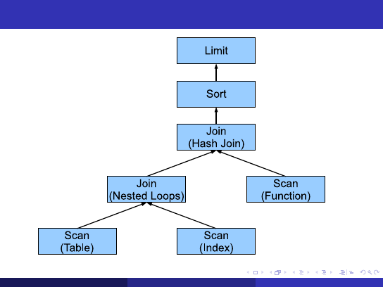
Expressing the Physical Algebra
Query Plans
The operators of the physical algebra are the techniques available for
query evaluation
Scan methods, join methods, sorts, aggregation operations, . . .
No simple relationship between logical operators and physical operators
Each operator has 0, 1 or 2 input relations, and 1 output relation
0 inputs: scans
2 inputs: joins, set operations
1 input: everything else
The operators are arranged in a tree
Data flows from the leaves toward the root
The “query plan” is simply this tree of operators
The output of the root node is the result of the query
Neil Conway (Truviso)
October 20, 2007
5 / 42

Typical Order Of Operations
Conceptual Plan Tree Structure
From leaf → root, a typical query plan conceptually does:
1
Scans: heap & index scans, function scans, subquery scans, . . .
2
Joins
3
Grouping, aggregation and HAVING
4
Sorting (ORDER BY)
5
Set operations
6
Projection (apply target list expressions)
In practice, various reordering and rewriting games, such as:
Pushdown: move operators closer to leaves to reduce data volume
Pullup: transform subqueries into joins
Choose lower-level operators to benefit upper-level operators
Neil Conway (Truviso)
October 20, 2007
7 / 42

The Iterator Model
Common Operator Interface
Most Postgres operators obey the same interface for exchanging data:
Init():
acquire locks, initialize state
GetNext():
return the next output tuple
Typically calls GetNext() on child operators as needed
Blocking operation
Optionally supports a direction (forward or backward)
ReScan():
reset the operator to reproduce its output from scratch
MarkPos():
record current operator position (state)
RestorePos():
restore previously-marked position
End():
release locks and other resources
Neil Conway (Truviso)
October 20, 2007
8 / 42

Properties of the Iterator Model
A Clean Design
Encodes both data flow and control flow
Operators simply pull on their inputs and produce results
Encapsulation: each operator needs no global knowledge
Disadvantages
1 tuple per GetNext() is inefficient for DSS-style queries
Operators can only make decisions with local knowledge
Synchronous: perhaps not ideal for distributed or parallel DBMS
Neil Conway (Truviso)
October 20, 2007
9 / 42

Pipelining
What Is Pipelining?
How much work must an operator do before beginning to produce results?
Some operators must essentially compute their entire result set before
emitting any tuples (e.g. external sort): “
materialization
”
Whereas other,
pipelinable
operators produce tuples one-at-a-time
Why Is It Important?
Lower latency
The operator may not need to be completely evaluated
e.g. cursors, IN and EXISTS subqueries, LIMIT, etc.
Pipelined operators require less state
Since materialized state often exceeds main memory, we may need to
buffer it to disk for non-pipelined operators
Plans with low startup cost sometimes > those with low total cost
Neil Conway (Truviso)
October 20, 2007
10 / 42

Basic Principles (Assumptions)
Disk I/O dominates query evaluation cost
Random I/O is more expensive than sequential I/O
. . . unless the I/O is cached
Reduce inter-operator data volume as far as possible
Apply predicates as early as possible
Assumes that predicates are relatively cheap
Also do projection early
TODO: pushdown grouping when possible
Fundamental distinction between plan-time and run-time
Planner does global optimizations, executor does local optimizations
No feedback from executor → optimizer
Neil Conway (Truviso)
October 20, 2007
11 / 42

Scan Evaluation
Sequential Scans
Simply read the heap file in-order: sequential I/O
Doesn’t necessarily match on-disk order, but it’s the best we can do
Must check heap at some point anyway, to verify that tuple is visible
to our transaction (“tqual”)
Evaluate any predicates that only refer to this table
The Problem
Must scan entire table, even if only a few rows satisfy the query
Neil Conway (Truviso)
October 20, 2007
12 / 42

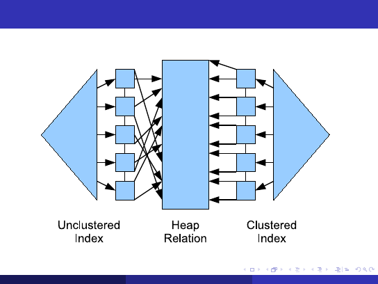
Index Scans
Basic Idea
Use a secondary data structure to quickly find the tuples that satisfy a
certain predicate
Popular index types include trees, hash tables, and bitmaps
Downsides
More I/Os needed: 1 or more to search the index, plus 1 to load the
corresponding heap page
Postgres cannot use “index-only scans” at present
Random I/O needed for both index lookup and heap page
Unless the index is clustered: index order matches heap order
Therefore, if many rows match predicate, index scans are inefficient
Index must be updated for every insertion; consumes buffer space
Neil Conway (Truviso)
October 20, 2007
13 / 42

B+-Tree Indexes
The Canonical Disk-Based Index For Scalar Data
On-disk tree index, designed to reduce # of disk seeks
1 seek per tree level; therefore, use a high branching factor: typically
100s of children per interior node
B != “binary”!
All values are stored in leaf nodes: interior nodes only for navigation
Tree height O(log
100
n): typically 5 or 6 even for large tables
Therefore, interior nodes are often cached in memory
Allows both equality and range queries: ≤, <, >, ≥, =
Leaf nodes are linked to one another
Highly optimized concurrent locking scheme
“Ubiquitous” even in 1979
Neil Conway (Truviso)
October 20, 2007
15 / 42

Bitmap Scans
Bitmap Scans
Basic idea: decouple scanning indexes from scanning the heap
1
For each relevant index on the target table:
Scan index to find qualifying tuples
Record qualifying tuples by setting bits in an in-memory bitmap
1 bit per heap tuple if there is space; otherwise, 1 bit per heap page
2
Combine bitmaps with bitwise AND or OR, as appropriate
3
Use the bitmap to scan the heap in order
Benefits
Reads heap sequentially, rather than in index order
Allows the combination of multiple indexes on a single table
More flexible than multi-column indexes
Neil Conway (Truviso)
October 20, 2007
16 / 42

Join Evaluation
Importance
Join performance is key to overall query processing performance
Much work has been done in this area
Toy Algorithm
To join R and S :
1
Materialize the Cartesian product of R and S
All pairs (r , s) such that r ∈ R, s ∈ S
2
Take the subset that matches the join key
. . . laughably inefficient: O(n
2
) space
Neil Conway (Truviso)
October 20, 2007
17 / 42

Nested Loops
Basic Algorithm
For a NL join between R and S on R.k = S .k:
for each tuple r in R:
for each tuple s in S with s.k = r.k:
emit output tuple (r,s)
Terminology: R is the
outer
join operand, S is the
inner
join operand.
Equivalently: R is
left
, S is
right
.
Simplest Feasible Algorithm
Only useful when finding the qualifying R and S tuples is cheap, and there
are few such tuples
R and S are small, and/or
Index on R.k, join key (or other predicates) is selective
Neil Conway (Truviso)
October 20, 2007
18 / 42

Sort-Merge Join
Basic Algorithm
For a SM join between R and S on R.k = S .k:
sort R on R.k
sort S on S.k
forboth r in R, s in S:
if r.k = s.k:
emit output tuple (r,s)
(Duplicate values make the actual implementation more complex.)
The Problem
This works fine when both R and S fit in memory
. . . unfortunately, this is typically not the case
Neil Conway (Truviso)
October 20, 2007
19 / 42

Option 1: Index-based Sorting
Avoid An Explicit Sort
Traversing leaf level of a B+-tree yields the index keys in order
Produce sorted output by fetching heap tuples in index order
NB: We can’t use a bitmap index scan for this purpose!
Downsides
Requires 2 I/Os: one for index page, one for heap page (to check
visibility)
Leaf-level is often non-contiguous on disk → random I/O
Unless index order matches heap order (clustered index), needs
random I/O to read heap tuples as well
Neil Conway (Truviso)
October 20, 2007
20 / 42


Option 2: External Sorting
Goal
Sort an arbitrary-sized relation using a fixed amount of main memory
Arbitrary disk space
Optimize to reduce I/O requirements
Not necessarily the number of comparisons!
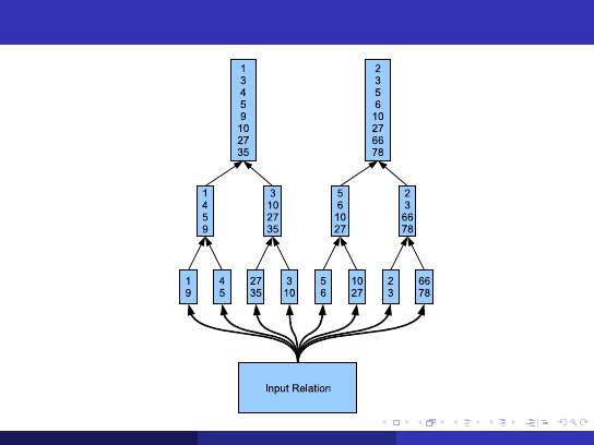
External Merge Sort
Divide the input into
runs
, sort each run in-memory, write to disk
Recursively merge runs together to produce longer sorted runs
Eventually, a single run contains the entire sorted output
Neil Conway (Truviso)
October 20, 2007
22 / 42

Option 2: External Sorting
Goal
Sort an arbitrary-sized relation using a fixed amount of main memory
Arbitrary disk space
Optimize to reduce I/O requirements
Not necessarily the number of comparisons!
External Merge Sort
Divide the input into
runs
, sort each run in-memory, write to disk
Recursively merge runs together to produce longer sorted runs
Eventually, a single run contains the entire sorted output
Neil Conway (Truviso)
October 20, 2007
22 / 42

Simple Algorithm
External Sort, v1
-- run generation phase
while (t = getNext()) != NULL:
add t to buffer
if buffer exceeds work_mem:
sort buffer
write to run file, reset buffer
-- merge phases
while > 1 run:
for each pair of runs:
merge them to into a single sorted run
Neil Conway (Truviso)
October 20, 2007
24 / 42

Optimizing Run Generation
Optimization Goals
Forms tree: height is # of merge phases, leaf level is # of initial runs
We read and write the entire input for each tree level → try to reduce
tree height
Replacement Selection
Simple approach: read input until work mem is reached, then sort and
write to temp file
Better: read input into an in-memory heap. Write tuples to temp file
as needed to stay under work mem
Next tuple to be written to a run is the smallest tuple in the heap that
is greater than the last tuple written to that run
Result: more comparisons, but runs are typically twice as large
Neil Conway (Truviso)
October 20, 2007
25 / 42

Optimizing The Merge Phases
Simple Approach
Merge sorted runs in pairs, yielding a binary tree (fan-in = 2)
To reduce tree height, maximize
fan-in
: merge > 2 runs at a time
Better Approach
1
Read the first tuple from each input run into an in-memory heap
2
Repeatedly push the smallest tuple in the heap to the output run;
replace with the next tuple from that input run
Optimizing I/O
Very sub-optimal I/O pattern: random reads from input runs
Therefore, use additional work mem to buffer each input run: alternate
between prereading to fill inputs and merging to write output
Tradeoff
: larger buffers optimizes I/O, but reduces fan-in
Neil Conway (Truviso)
October 20, 2007
26 / 42

Further Refinements
Don’t Materialize Final Merge Phase
Skip final merge phase: produce output from the penultimate set of runs
Small Inputs
Many sorts are small → just buffer in work mem and quicksort
Avoid Redundant Sorts
If the input is already sorted, we can avoid the sort altogether
A sizable portion of the planner is devoted to this optimization
(“interesting orders”)
Neil Conway (Truviso)
October 20, 2007
27 / 42

Bounded Sort
A Special Case: LIMIT
Can we do better, if we know at most k tuples of the sort’s output will be
needed?
8.3 Feature
If k is small relative to work mem, no need to go to disk at all
Instead, keep k highest values seen-so-far in an in-memory heap
Benefits:
No need to hit disk, even for large inputs
O(n · log k) comparisons rather than O(n · log n)
Neil Conway (Truviso)
October 20, 2007
28 / 42

Hash Join
Classic Hash Join Algorithm
For a HJ between R and S on R.k = S .k:
-- build phase
for each tuple r in R:
insert r into hash table T with key r.k
-- probe phase
for each tuple s in S:
for each tuple r in bucket T[s.k]:
if s.k = r.k:
emit output tuple (T[s.k], s)
Pick R to be the smaller input.
The Problem
What if we can’t fit all of R into memory?
Neil Conway (Truviso)
October 20, 2007
29 / 42

Simple Overflow Avoidance
Simple Algorithm
for each tuple r in R:
add r to T with key r.k
if T exceeds work_mem:
probe S for matches with T on S.k
reset T
-- final merge phase
probe S for matches with T on S.k
The Problem
Works fairly well, but reads S more times than necessary
If we’re going to read S multiple times, we can do better
Neil Conway (Truviso)
October 20, 2007
30 / 42

Grace Hash Join
Algorithm
Choose two orthogonal hash functions, h
1
and h
2
Read in R and S . Form k partitions by hashing the join key using h
1
and write out the partitions
Then hash join each of the k partitions independently using h
2
Two matching tuples must be in the same partition
If a partition does not fit into memory, recursively partition it via h
3
Problems
Sensitive to the distribution of input data: partitions may not be
equal-sized
Therefore, we want to maximize k, to increase the chance that all
partitions fit in memory
Inefficient if R fits into memory: no need to partition at all
Neil Conway (Truviso)
October 20, 2007
31 / 42

Hybrid Hash Join
A Small But Important Refinement
Treat partition 0 specially: keep it in memory
Therefore, divide available memory among partition 0, and the output
buffers for the remaining k partitions
Partition Sizing
If we have B buffers in work mem, we can make at most B partitions
If any of the partitions is larger than B, we need to recurse
Tradeoff: devote more memory to partition 0, or to maximizing the
number of partitions?
Neat Trick
When joining on-disk partitions, if |S
k
| < |R
k
|, switch them
Neil Conway (Truviso)
October 20, 2007
32 / 42

Aggregate Evaluation
Basic Task
1
Form groups (“map”)
Collect rows with the same grouping key together
2
Evaluate aggregate functions for each group (“reduce”)
Similar techniques needed for duplicate elimination (DISTINCT, UNION).
Aggregate API
For each aggregate, in each group:
1
s = initcond
2
For each value v
i
in the group:
s = sfunc(s, v
i
)
3
final = ffunc(s)
Neil Conway (Truviso)
October 20, 2007
33 / 42

Grouping by Sorting
Simple Idea
1
Take the inputs in order of the grouping key
Sort if necessary
2
For each group, compute aggregates over it and emit the result
Naturally pipelined, if we don’t need an external sort.
Neil Conway (Truviso)
October 20, 2007
34 / 42

Grouping by Hashing
Simple Idea
1
Create a hash table with one bucket per group
2
For each input row:
Apply hash to find group
Update group’s state value accordingly
Inherently non-pipelinable. Typically performs well for small numbers of
distinct groups.
The Problem
What happens if the size of the hash table grows large?
That is, if there are many distinct groups
At present, nothing intelligent — the planner does its best to avoid
hashed aggregation with many distinct groups
FIXME
Neil Conway (Truviso)
October 20, 2007
35 / 42

Set Operations
Two Requirements
1
Duplicate elimination (unless ALL is specified)
2
Perform set operation itself: UNION, INTERSECT, EXCEPT
Implementation
Both requirements can be achieved by concatenating the inputs together,
then sorting to eliminate duplicates
For UNION ALL, we can skip the sort
TODO: consider hashing?
TODO: consider rewriting set operations → joins
Neil Conway (Truviso)
October 20, 2007
36 / 42

Duality of Sorting and Hashing
A Nice Idea, due to Graefe, Linville and Shapiro (1994)
Both algorithms are simple for small inputs
Quicksort, classic hash join
Use divide-and-conquer for large inputs: partition, then merge
Hashing:
partition on a logical key (hash function), then merge
on a physical key (one partition at a time)
Sorting:
partition on a physical key (position in input), then
merge on a logical key (sort key)
I/O pattern: hashing does random writes and sequential reads,
whereas sorting does random reads and sequential writes
Hashing can be viewed as radix sort on a virtual key (hash value)
Neil Conway (Truviso)
October 20, 2007
37 / 42

Reading EXPLAIN
EXPLAIN pretty-prints the plan chosen for a query
For each plan node: startup cost, total cost, and result set size
Estimated cost is measured in units of disk I/Os, with fudge factors for
CPU expense and random vs. sequential I/O
A node’s cost is
inclusive
of the cost of its child nodes
EXPLAIN ANALYZE also runs the query and gathers runtime stats
Runtime cost is measured in elapsed time
How many rows did an operator
actually
produce?
Where is the bulk of the query’s runtime
really
spent?
Did the planner’s estimates actually match reality?
Most common planner problem: misestimating result set sizes
When debugging for planner mistakes,
work from the leaves up
(And of course, be sure to run ANALYZE)
Neil Conway (Truviso)
October 20, 2007
38 / 42

Example Query
SELECT t2.id, t1.name
FROM t1, t2
WHERE t1.tag_id = t2.tag_id
AND t2.field1 IN (5, 10, 15, ...)
AND t2.is_deleted IS NULL;
Neil Conway (Truviso)
October 20, 2007
39 / 42

EXPLAIN ANALYZE Output
Merge Join
(cost=18291.23..21426.96 rows=3231 width=14)
(actual time=14.024..212.427 rows=225 loops=1)
Merge Cond: (t1.tag_id = t2.tag_id)
->
Index Scan using t1_pkey_idx on t1
(cost=0.00..2855.74 rows=92728 width=14)
(actual time=0.041..115.231 rows=54170 loops=1)
->
Sort
(cost=18291.23..18299.31 rows=3231 width=8)
(actual time=13.967..14.289 rows=225 loops=1)
Sort Key: t2.tag_id
Sort Method:
quicksort
Memory: 26kB
->
Bitmap Heap Scan on t2
(cost=5659.07..18102.90 rows=3231 width=8)
(actual time=12.731..13.493 rows=225 loops=1)
Recheck Cond: ((field1 = ANY (’{5, 10, 15, ...}’::integer[]))
AND (is_deleted IS NULL))
->
Bitmap Index Scan on t2_field1_idx
(cost=0.00..5658.26 rows=3231 width=0)
(actual time=12.686..12.686 rows=225 loops=1)
Index Cond: (field1 = ANY (’{5, 10, 15, ...}’::integer[]))
Total runtime: 212.939 ms
Neil Conway (Truviso)
October 20, 2007
40 / 42

Conclusion
Thank you.
Any questions?
Neil Conway (Truviso)
October 20, 2007
41 / 42

References
Classic survey paper on query evaluation techniques:
G. Graefe. Query Evaluation Techniques for Large Databases. In ACM Computing
Surveys, Vol. 25, No. 2, June 1993.
The duality of sorting and hashing, and related ideas:
G. Graefe, A. Linville, L. D. Shapiro. Sort versus hash revisited. IEEE Transactions
on Knowledge and Data Engineering, 6(6):934–944, December 1994.
Hybrid hash join:
L. D. Shapiro. Join Processing in Database Systems with Large Main Memories.
ACM Transactions on Database Systems, Vol. 11, No. 3, 1986.
Postgres’ external sorting implementation is based on Knuth:
D. Knuth. The Art of Computing Programming: Sorting and Searching, vol. 3.
Addison-Wesley, 1973.
An exhaustive survey on DBMS sorting techniques:
G. Graefe. Implementing Sorting in Database Systems. In ACM Computing
Surveys, Vol. 38, No. 3, 2006.
Neil Conway (Truviso)
October 20, 2007
42 / 42
Document Outline
Wyszukiwarka
Podobne podstrony:
5 Techniki in situ
Techniki in vitro
07 AI Techniques in Games
Dane Rudhyar THE PRACTICE OF ASTROLOGY AS A TECHNIQUE IN HUMAN UNDERSTANDING
FIDE Trainers Surveys 2011 12 Alexander Beliavsky Winning and Defending Technique in the Queen Endin
Jünger, Ernst Technik In Der Zukunftsschlacht (Militaer Wochenblatt, 1921)
SzczygielskiStopa Usage of new soil improvement techniques in road embankment constructions
Advanced Metamorphic Techniques in Computer Viruses
Key Concepts & Techniques in GIS
Executive Decision Those Fat Cats in Congress
Learning to Detect Malicious Executables in the Wild
Learning to Detect and Classify Malicious Executables in the Wild
Alyx J Shaw A Strange Place in Time 3 The Merry Executioner Returns np#,hdr
Static Detection of Malicious Code in Executable Programs
IMAD In Execution Malware Analysis and Detection
Alyx J Shaw A Strange Place in Time 3 The Merry Executioner Returns c
Alyx J Shaw A Strange Place in Time 3 The Merry Executioner Returns
więcej podobnych podstron