Integration of edge-diffraction calculations and geometrical-acoustics modeling

Paul T. Calamia

Dept. of Computer Science, Princeton University, Princeton, NJ, USA, e-mail: [e-mail]

U. Peter Svensson

Acoustics Group, Dept. of Electronics and Telecommunications, Norwegian University of Science and Technology,

Trondheim, Norway, e-mail: [e-mail]

Thomas A. Funkhouser

Dept. of Computer Science, Princeton University, Princeton, NJ, USA, e-mail: [e-mail]

In time-domain simulations of sound propagation and/or scattering, it is possible to model the geometrical-
acoustics (GA) components and the edge-diffraction components separately and combine the results into a
“total” impulse response. However, such separate calculations can limit the efficiency and accuracy of the
simulations because the two components are not independent. This paper presents an integrated approach
for time-domain acoustic modeling in which intermediate values normally utilized only in diffraction cal-
culations are exploited in finding the GA components as well. Specifically, it is shown how to detect the
existence of first-order specular reflections and an unobstructed direct-sound path using source and receiver
locations specified in edge-aligned cylindrical coordinates. The benefits of the method are described for
general modeling cases, as well as for specific source/receiver configurations in which the receiver is lo-
cated on or near a specular-zone or shadow-zone boundary. Particular attention is paid to the zone-boundary
cases, where this method is well suited to ensure continuity of the sound field across the boundary.

1

Introduction

Time-domain simulations often are used in room-
acoustics modeling because they allow for intuitive eval-
uation of the contributions of individual components
to the sound field, and they provide results which can
be analyzed easily with standardized parameters and
through auralization. Geometrical-acoustics (GA) tech-
niques have long been the basis for such simulations,
but are known to be incomplete and inaccurate, partic-
ularly at low frequencies, in part because they fail to in-
clude diffraction. A straightforward approach to remedy
this failure involves augmenting GA results with edge-
diffraction calculations, e.g. as is done in [1] and [2].
However, separate calculations of these two components
can limit the efficiency and accuracy of the simulations
because the components are not independent.

The relationship between the GA and diffraction compo-
nents can be seen most easily for a simulation in which
the receiver is located on or near a specular-zone or
shadow-zone boundary. At these boundaries the associ-
ated GA components undergo discontinuities when they
become obstructed (or unobstructed) by a surface, and
the diffraction components compensate for these discon-
tinuities such that the combined response is continuous
across the boundary. The proper combination of the two
components requires that both be simulated with a high
degree of numerical accuracy, and incorrect detection or
modeling of either can introduce large errors.

In this paper, we present an integrated approach for time-
domain acoustic modeling in which intermediate values

normally utilized only in diffraction calculations are ex-
ploited in finding the GA components as well. Specif-
ically, we show how to detect the existence of first-
order specular reflections and an unobstructed direct-
sound path using source and receiver locations specified
in edge-aligned cylindrical coordinates. This method can
be used for arbitrary source and receiver configurations,
but is particularly well suited for use with receivers at
or near zone boundaries because it ensures a consistent,
physically correct combination of components.

The remainder of this paper is organized as follows. Sec-
tion 2 contains a brief review of GA components and
edge diffraction, the latter based on calculations derived
from the Biot-Tolstoy-Medwin formulation. Section 3
describes our integrated modeling approach. Section 4
describes the benefits of our approach, and Section 5 con-
tains conclusions and plans for further work.

2

Sound-Field Components

Given a sound source, receiver, and an object or environ-
ment comprising planar, faceted surfaces, it is possible to
decompose the associated sound field into geometrical-
acoustics components and edge-diffraction components
[3]. The former group consists of the direct sound and
specular reflections, and the latter consists of contribu-
tions that result from sound scattered by free edges, cor-
ners, or wedges. The two groups are often addressed sep-
arately in numerical simulations.

Forum Acusticum 2005 Budapest

Calamia, Svensson, Funkhouser

2.1

Geometrical Acoustics

Simulations based on geometrical acoustics rely on ray
theory, i.e. the approximation that sound propagates be-
tween two points along straight, ray-like paths. Thus,
an unoccluded linear path between a source and receiver
is sufficient to model the direct sound, and specular re-
flections can be simulated by piecewise linear paths that
obey Snell’s Law when they encounter flat, reflecting sur-
faces. Such ray-like behavior is only correct when the
dimensions of the reflecting surface are infinitely larger
than the wavelength of the incident sound, and thus GA
methods are particularly inaccurate when used with small
reflecting surfaces or low-frequency (long-wavelength)
sound. GA components can be calculated with a number
of different methods, including the image-source method
(ISM) [4], ray tracing [5], and beam tracing [6].

2.2

Edge Diffraction

For finite surfaces and low frequencies, edge diffraction
must be included to simulate the reflection/scattering be-
havior accurately. A popular technique to model diffrac-
tion involves the Biot-Tolstoy-Medwin (BTM) formula-
tion, an exact, continuous-time expression for the diffrac-
tion by a rigid wedge [7, 8].

1

Our modeling approach em-

ploys a discrete-time expression derived from the BTM
formulation which gives the edge-diffraction impulse re-
sponse (IR) as a line integral along the edge.

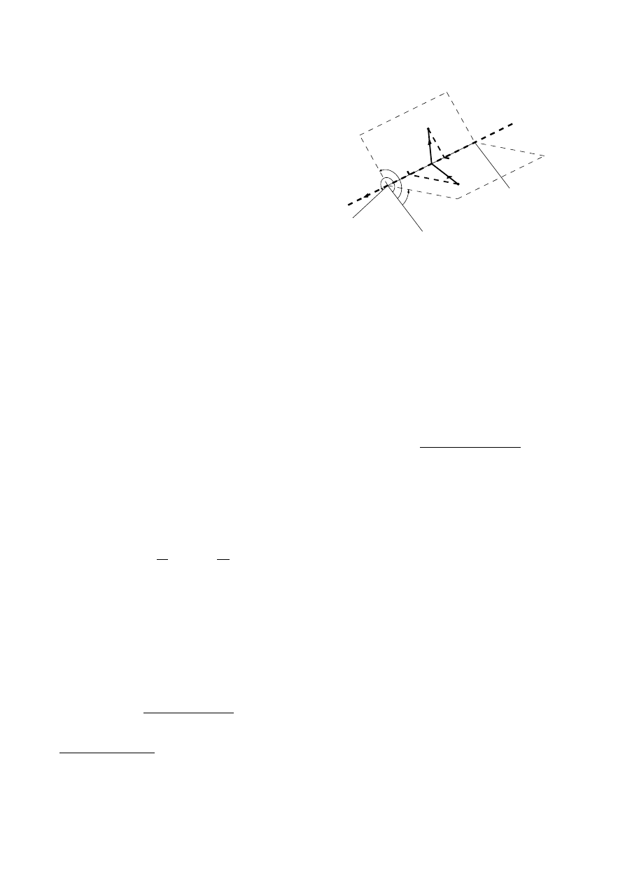
Consider a rigid wedge as shown in Figure 1, with a
point source S and a receiver R whose positions are given
with edge-aligned cylindrical coordinates (r

S

, θ

S

, z

S

)

and (r

R

, θ

R

, z

R

), respectively. The discrete-time edge-

diffraction IR for such a wedge, as presented in [3], is

h(n) =

−

ν

4π

4

i=1

z

n,2

z

n,1

β

i

ml

dz,

(1)

where ν = π/θ

W

is the wedge index, θ

W

is the open

wedge angle, and m and l are the distances from the
source to the edge point and the receiver to the edge point,
respectively. The integration limits z

n,1

are z

n,2

are the

result of area-sampling the continuous-time formulation,
and represent points on the edge which correspond to
travel times (n

± 0.5)/f

S

for sample n and sampling fre-

quency of f

S

. The functions β

i

are

β

i

=

sin(νϕ

i

)

cosh(νη)

− cos(νϕ

i

)

,

(2)

where the angles ϕ

i

are

1

The complete solution for the wedge problem originally presented

in [7] includes both image reflections and diffraction from the wedge,
but the former are rarely included in BTM calculations.

S

R

m

l

r

S

r

R

z

S

z

R

θ

S

θ

R

θ

W

z

P

R

P

S

Figure 1: Wedge geometry and coordinate system. Lo-
cations are specified in cylindrical coordinates where r is
the radial distance from the edge, θ is measured from one
of the two wedge faces, and the z-axis is aligned with the
edge. P

S

and P

R

are virtual half-planes that contain S

and R, respectively, and the edge.

ϕ

1

= π + θ

S

+ θ

R

,

ϕ

2

= π + θ

S

− θ

R

,

ϕ

3

= π

− θ

S

+ θ

R

,

ϕ

4

= π

− θ

S

− θ

R

,

(3)

and the auxiliary function η is

η = cosh

−1

ml + (z

− z

S

)(z

− z

R

)

r

S

r

R

.

(4)

The shortest path from the source to the receiver through
the line that contains the edge goes through the so-called
apex point on that line, and this apex point may or may
not be contained within the physical edge. If it is within
the edge, the onset sample of the diffraction IR is deter-
mined by the path through the apex point. If it is not,
the onset is determined by the shorter of the two paths
through the endpoints of the physical edge.

In general, the numerical integration of Eq.

(1) for

each sample is straightforward, but the edge-diffraction
IR is subject to a singularity in its first sample when
cosh(νη) = cos(νϕ

i

) = 1, as can be seen in Eq. (2). The

singularity is present when two conditions hold. First, the
apex point must be contained within the physical edge,
and thus the onset time (sample) is dictated by the path
through this point (for which cosh(νη) = 1). Second, the
receiver must be located on a specular-zone or shadow-
zone boundary (for which cos(νϕ

i

) = 1 for one or two

ϕ

i

angles). For such cases, analytical approximations are

described in [9] that are valid for the first sample of the
discrete-time IR. At each zone boundary, the singular-
ity in the diffraction component is necessary to compen-
sate for the discontinuity in the associated geometrical-
acoustics component (direct sound or specular reflection)
and thus to maintain a continuous sound field across the
zone boundary.

Forum Acusticum 2005 Budapest

Calamia, Svensson, Funkhouser

3

Integrated Modeling Approach

Rather than calculate the GA and diffraction components
separately, it is possible to exploit intermediate values
normally used only in diffraction calculations to find the
GA components as well. In particular, the ϕ

i

angles de-

fined in Eq. (3) contain sufficient information to detect
the existence of first-order specular reflections and an un-
obstructed direct-sound path. Additionally, the radial and
angular coordinates of the source and receiver, r

S

, r

R

,

θ

S

, and θ

R

, can be used to locate the reflection point on a

surface which is found to cause a specular reflection.

Our method assumes that the environment/model is
stored as a triangle mesh, with explicit lists of the faces,
edges, and vertices. A single pass over the list of edges is
used to generate and store the diffraction parameters, and
to calculate the diffraction components of the sound field.
For edges that occur at the intersection of two faces (i.e.
at corners and wedges), the diffraction parameters must
be measured relative to both faces, since either or both
could occlude the direct sound or create a specular reflec-
tion. The actual diffraction calculations for the edge can
be made with either set of parameters. For edges that are
known not to diffract, e.g. those for which θ

W

= π/m

for integer values of m, the parameters must still be gen-
erated for use in detecting the GA components, but the
diffraction calculations can be skipped.

In a subsequent pass over the list of faces, the diffrac-
tion parameters are evaluated to determine whether or nor
each face obstructs the direct sound or creates a specular
reflection. Specifically, two counters are maintained for
each face, one with the number of its edges for which
ϕ

2

< 0 or ϕ

3

< 0 and one with the number of its edges

for which ϕ

4

> 0, and are updated during the pass over

the edges. As described below, a face obstructs the direct
sound if the value in its first counter is 3, and the face cre-
ates a specular reflection if the value in its second counter
is 3. For a face that creates a specular reflection, further
evaluation of the parameters is necessary to find the re-
flection point. Once a face has been found to obstruct the
direct sound, no other faces need to be tested for such an
obstruction. Once a specular reflection has been found
to be created by a face, no other faces in the same plane
need to be considered for reflections.

3.1

Direct Sound

To determine whether there is a clear direct-sound path
from the source to the receiver, each face in the model
must be considered as a possible occluder. This can be
done using ϕ

2

or ϕ

3

as defined in Eq. (3). Relative to a

single edge, the face will occlude the direct-sound path if
θ

S

and θ

R

differ by more than π, i.e. if π

−|θ

S

−θ

R

| < 0.

If θ

S

≤ θ

R

,

|θ

S

−θ

R

| = (θ

R

−θ

S

), thus occlusion occurs

S

R

1

R

2

ϕ

2

=

π

+

θ

S

−

θ

R

1

>

0

ϕ

2

=

π

+

θ

S

−

θ

R

2

<

0

(a)

ϕ

2

< 0

ϕ

2

> 0

ϕ

2

> 0

ϕ

2

> 0

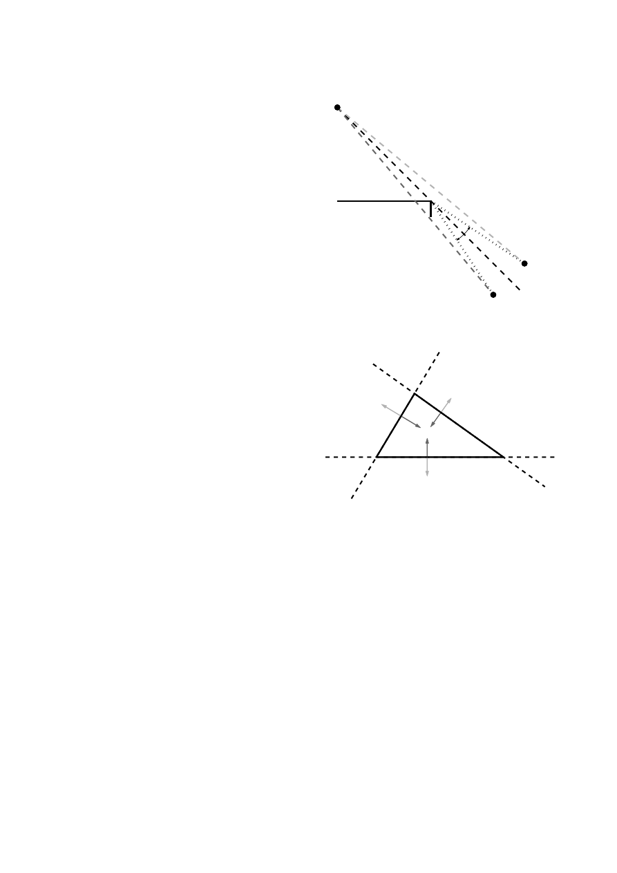
(b)

Figure 2: Checking for occlusion of the direct sound. (a)
The face under test is shown as a horizontal line, and the
edge under test comes out of the page. The diffraction
parameter ϕ

2

from Eq. (3) measures the angular distance

of the receiver from the shadow boundary. If ϕ

2

< 0

(e.g. for R

2

), the receiver is beyond the shadow boundary

relative to the edge under test. (b) If ϕ

2

< 0 for all three

edges of the face, the face occludes the direct sound.

when π

− (θ

R

− θ

S

) = π

− θ

R

+ θ

S

= ϕ

2

< 0. If

θ

S

> θ

R

,

|θ

S

− θ

R

| = (θ

S

− θ

R

), and occlusion occurs

when π

− (θ

S

− θ

R

) = π

− θ

S

+ θ

R

= ϕ

3

< 0. If the

appropriate value, ϕ

2

or ϕ

3

, is negative for all three edges

of a face, the face occludes the direct sound. An example
using ϕ

2

is shown in Figure 2.

This can be confirmed geometrically by the following,
using a case for which ϕ

2

is evaluated. Each edge of a

face is contained by an infinite line, and each such line
divides the plane of the face into two half-planes: one
which contains the face and one which does not. For a

Forum Acusticum 2005 Budapest

Calamia, Svensson, Funkhouser

given edge, ϕ

2

< 0 implies that that the line segment be-

tween the source and the receiver intersects the half-plane
that contains the face, as can be seen by the intersection
of the horizontal line representing the face and the line
segment between S and R

2

in Figure 2 (a). Once ϕ

2

has been evaluated for all three edges, the point at which
the path from the source to the receiver passes through
the plane of the face can be localized to the intersection
of three half-planes, each dictated by the sign of one ϕ

2

value. As seen in Figure 2 (b), the intersection of the
three half-planes defined by ϕ

2

< 0 for each edge is ex-

actly the face, and thus three negative values imply that
the path from the source to the receiver goes through the
face, i.e. is occluded by it. No other combination of three
half-planes contains any portion of the face, so a single
case of ϕ

2

> 0 for a given face eliminates that face from

the list of possible occluders of the direct sound.

3.2

First-Order Specular Reflections

3.2.1

Finding Reflecting Surfaces

The test for a specular reflection from a face involves
evaluating ϕ

4

for each of the face’s three edges. As de-

fined in Eq. (3), ϕ

4

= π

− θ

S

− θ

R

, and thus it measures

the angular distance of the receiver (θ

R

) from the spec-

ular boundary (π

− θ

S

). As shown in Figure 3, when

ϕ

4

> 0, the receiver is within the specular zone rela-

tive to the edge from which θ

S

and θ

R

are measured. If

ϕ

4

> 0 for all edges of a face, the face creates a specular

reflection. Note that the evaluation of ϕ

4

need only be

done if both θ

S

< π and θ

R

< π. If either is greater than

π, there can be no specular reflection from the reference
face.

A similar geometric argument holds in this case as well.
For a given face and one of its edges, ϕ

4

> 0 implies that

that the point of specular reflection lies in the half-plane
that contains the face, as can be seen by the reflection
path between S and R

1

in Figure 3 (a). The three ϕ

4

values localize the reflection point to the intersection of
three half-planes, and this intersection for three positive
ϕ

4

values is exactly the face as shown in Figure 3 (b).

3.2.2

Finding Reflection Points

Once a surface has been found to create a specular re-
flection, it is also possible to locate the point of reflection
using the diffraction parameters. This method involves
deriving the barycentric coordinates of the point within
the reflecting (triangular) surface, and is similar to one
which is commonly used in computer graphics, specifi-
cally in ray-tracing applications, to find line-triangle in-
tersections.

To find the coordinates of the specular reflection point, it

S

R

1

R

2

ϕ

4

=

π

−

θ

S

−

θ

R

1

>

0

ϕ

4

=

π −

θ

S

−

θ

R

2

<

0

(a)

ϕ

4

> 0

ϕ

4

< 0

ϕ

4

< 0

ϕ

4

< 0

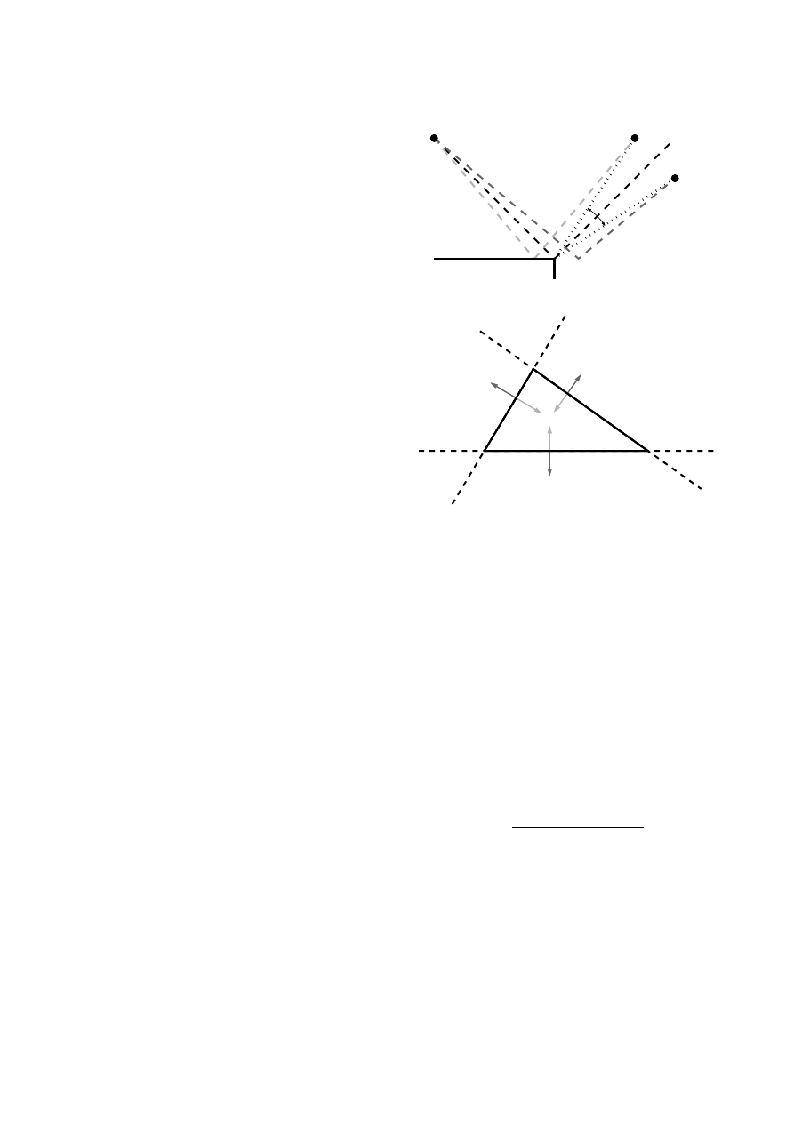
(b)

Figure 3: Confirming a specular reflection. (a) The face
under test is shown as a horizontal line, and the edge un-
der test comes out of the page. The diffraction parameter
ϕ

4

= π

− θ

S

− θ

R

measures the angular distance of the

receiver from the specular boundary. If ϕ

4

> 0 (e.g. for

R

1

), the receiver is within the specular zone relative to

the edge under test. (b) If ϕ

4

> 0 for all three edges of a

triangular face, the face creates a specular reflection.

is helpful to consider first a 2D example as in Figure 4
(a). Given a source, receiver, and a line segment, the goal
is to find the distance x of the reflection point from the
end of the segment in terms of the diffraction parameters
r

S

, r

R

, θ

S

, and θ

R

. With the constraint that α

1

= α

2

(true for a specular reflection), x is given by the equation

x =

r

S

r

R

sin(θ

S

+ θ

R

)

r

S

sin(θ

S

) + r

R

sin(θ

R

)

.

(5)

For a 3D case, consider the source S, receiver R, and tri-
angular face

ABC in Figure 4 (b) for which ϕ

4

> 0

for all three edges. The first-order specular reflection
path from S to R must go through a point P in the in-
terior of the face, and the value x in Eq. (5) corresponds
to the perpendicular distance from P to the edge from
which r

S

, r

R

, θ

S

, and θ

R

are measured. Therefore, us-

ing side BC as a reference yields x

BC

, using side CA

yields x

CA

, and using side AB yields x

AB

. The triple

(x

BC

, x

CA

, x

AB

) represents the location of P in exact

Forum Acusticum 2005 Budapest

Calamia, Svensson, Funkhouser

trilinear coordinates. This triple can be converted into
barycentric coordinates (t

1

, t

2

, t

3

) [10], where

t

1

=

x

BC

· a

n

,

t

2

=

x

CA

· b

n

,

t

3

=

x

AB

· c

n

,

(6)

a, b, and c are the lengths of the sides of the face as shown
in Figure 4 (b), and

n = a

· x

BC

+ b

· x

CA

+ c

· x

AB

.

(7)

Using the known Cartesian coordinates of the triangle
vertices A, B, and C, the Cartesian coordinates of the
specular reflection point can be found with the equation

P = A

· t

1

+ B

· t

2

+ C

· t

3

.

(8)

The value r

S

sin(θ

S

) in Eq. (5) is the distance from the

source to the plane containing the face, and r

R

sin(θ

R

)

is the distance from the receiver to that plane. These
distances are constant for all edges of a face, and thus
must be calculated only once per face.

The value

r

S

r

R

sin(θ

S

+ θ

R

) must be computed for each edge.

4

Discussion

4.1

Accuracy

The benefit of our method in terms of simulation accu-
racy is most pronounced for a receiver which is on a
zone boundary. For such a case involving a specular-zone
boundary, the reflection point lies on an edge of a surface,
and the reflection arrival time and diffraction onset time
are equal. To maintain a continuous sound field across
the boundary, the combined amplitude of the specular re-
flection and the first sample of the diffraction IR should
be one half the expected reflection value [9]. Because
ϕ

4

= 0 for such a case, it is easy to note such a condi-

tion when processing the related edge (using a small to
avoid numerical inaccuracies), and adjust the diffraction
and specular reflection strengths accordingly to achieve
the proper amplitude. However, using separate GA and
diffraction methods, such a condition would have to be
found by the two methods consistently and accurately.
In particular, the technique for finding the specular re-
flections would be required to find path/edge intersec-
tions within the same as the diffraction model to ensure
proper amplitudes for both components. Failure to detect
and integrate the two components properly could lead to
a response with double the correct amplitude, zero ampli-
tude due to destructive interference, or incorrect diffrac-
tion polarity.

S

R

r

S

r

R

θ

S

θ

R

α

1

α

2

x

(a)

A

B

C

P

x

AB

x

BC

x

CA

c

a

b

S

R

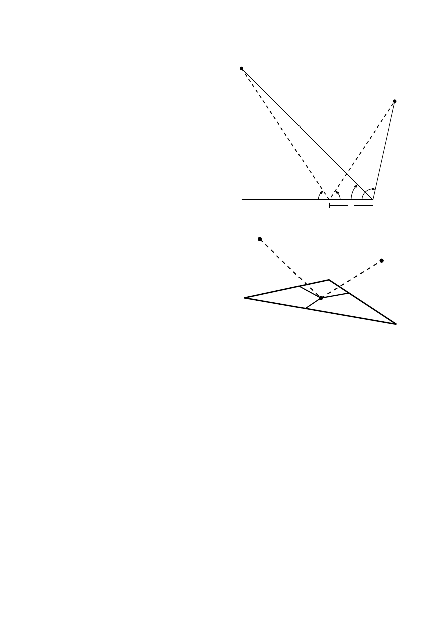
(b)

Figure 4: Finding the reflection point P . (a) 2D geometry
used to find the distance x of P from an edge. (b) Values
x

AB

, x

BC

, and x

CA

, each calculated with Eq. (5) rela-

tive to one of the three edges, give the location of P in
exact trilinear coordinates. These can be converted into
barycentric coordinates using Eqs. (6) and (7), which in
turn give the Cartesian coordinates of P through Eq. (8).

4.2

Efficiency

Our method also provides improved efficiency over the
image-source method (although methods such as beam
tracing that employ spatial subdivision schemes can de-
tect specular reflections more efficiently). With the ISM,
faces are evaluated for specular reflections by: mirroring
the source about the plane containing the face to create an
image source; finding the intersection of that plane with
the line between the image source and the receiver; de-
termining whether the intersection point is inside (valid
reflection) or outside (invalid reflection) the boundaries
of the face. With our method, the existence of a reflec-
tion is determined by simply examining the ϕ

4

counter

for each face. If the counter value is less than 3, nothing

Forum Acusticum 2005 Budapest

Calamia, Svensson, Funkhouser

more needs to be done. If the counter value is 3, we can
either use the method described in Section 3.2.2 to find
the exact reflection point, or follow the steps used in the
ISM. For the latter, we need only carry out the first two
steps. Since the surface is known to create a valid spec-
ular reflection, the intersection of the path between the
image source and receiver and the reflecting plane must
be inside the boundaries of the face, so the final step is
not necessary.

5

Conclusions

This paper describes a time-domain method for acoustic
modeling which integrates geometrical-acoustics compo-
nents and edge diffraction. Parameters generated for the
diffraction calculations are also used to confirm an un-
obstructed direct-sound path and to find first-order spec-
ular reflections, thus eliminating the need for a sepa-
rate GA technique such as the image-source method.
This approach is particularly well suited for use with re-
ceivers at or near specular-zone and shadow-zone bound-
aries, where the proper combination of GA and diffrac-
tion components is essential to ensure a physically accu-
rate, continuous sound field across the boundary.

One aspect of this work that demands further study is
the need for visibility checks for the specular reflec-
tions. In traditional GA systems, rays are cast along each
reflection-path segment, and tested for intersection with
the surfaces in the model. If one of these rays intersects
a surface before arriving at the expected reflecting sur-
face, the reflection is considered invalid. Such a method
could be included in our system. Another possibility is to
check for occlusions for each segment of a reflection path
with the approach described in Section 3.1 for the direct
sound. A reflection path S

→ P → R could be evaluated

by first searching for obstructions with S as the source
and P as the receiver, and then for obstructions with P
as the source and R as the receiver. It may be possible
to incorporate such visibility checks into the calculations
for higher-order sound-field components.

A second direction for further work involves extending
this method beyond first-order specular reflections and
diffraction. As in the first-order case, diffraction com-
pensates for discontinuities at higher-order specular-zone
boundaries, so our integrated method should be applica-
ble. However, additional tests will be necessary to val-
idate each segment of higher-order specular reflection
path.

Finally, it should be possible to use a similar approach
with convex faces other than triangles, with a modified
process for finding specular reflection points. This could
increase the method’s efficiency by reducing the number
of edges and faces to process.

Acknowledgement

This work has been funded in part by a Norwegian Mar-
shall Fund Award from the Norway-America Associa-
tion, the Acoustics Research Centre project from the
Research Council of Norway, and the National Science
Foundation (CCR-0093343).

References

[1] R. R. Torres, U. P. Svensson, and M. Kleiner, “Com-

putation of edge diffraction for more accurate room
acoustics auralization,” J. Acoust. Soc. Am., vol.
109, pp. 600–610, 2001.

[2] V. Pulkki, T. Lokki, and L. Savioja, “Implemen-

tation and visualization of edge diffraction with
image-source method,” in Proc. 112th Audio Engi-
neering Society Convention, 2002.

[3] U. P. Svensson, R. I. Fred, and J. Vanderkooy, “An-

alytic secondary source model of edge diffraction
impulse responses,” J. Acoust. Soc. Am., vol. 106,
pp. 2331–2344, 1999.

[4] J. Borish, “Extension of the image model to arbi-

trary polyhedra,” J. Acoust. Soc. Am., vol. 75, pp.
1827–1836, 1984.

[5] A. Krokstad, S. Strøm, and S. Sørsdal, “Calculating

the acoustical room response by the use of a ray-
tracing technique,” J. Sound Vib., vol. 8, pp. 118–
125, 1968.

[6] T. Funkhouser, I. Carlbom, G. Elko, G. Pingali,

M. Sondhi, and J. West, “A beam tracing ap-
proach to acoustic modeling for interactive virtual
environments,” in ACM Computer Graphics, SIG-
GRAPH’98 Proceedings, 1998, pp. 21–32.

[7] M. A. Biot and I. Tolstoy, “Formulation of wave

propagation in infinite media by normal coordinates
with an application to diffraction,” J. Acoust. Soc.
Am., vol. 29, pp. 381–391, 1957.

[8] H. Medwin, “Shadowing by finite noise barriers,” J.

Acoust. Soc. Am., vol. 69, pp. 1060–1064, 1981.

[9] U. P. Svensson and P. Calamia, “Edge-diffraction

impulse responses near specular-zone and shadow-
zone boundaries,” Submitted to Acustica/Acta Acus-
tica, Dec. 2004.

[10] E. W. Weisstein, “Trilinear Coordinates,” From

MathWorld–A Wolfram Web Resource. Avail-
able:

http://mathworld.wolfram.com/TrilinearCo-

ordinates.html