Energia kinetyczna w ruchu płaski Wykład 15

Ruch płaski uzyskany, traktując ten ruch jako złożony z ruchu postępowego unoszenia z prędkością środka masy

V_u= V_C i ruchu obrotowego względnego dookoła prostej

przechodzącej przez środek masy C, prostopadłej do płaszczyzny kierującej.

y z

V_w ω

0 y

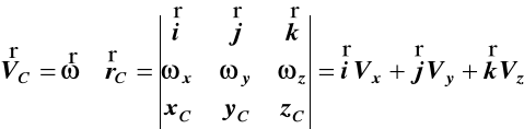
C r V r_C

A V_C C

r_C V_C r

0 x x A

V

Rys. 48 V_w = w, V_C = V_u = u, V = w +V_C

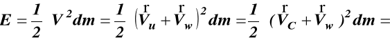
(a)

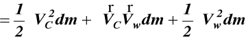
(b)

(c)

ponieważ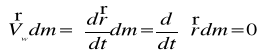

położenie środka masy względem środka masy

równa się zero.

Podstawiając (b) i (c) do (a) otrzymujemy

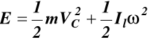
gdzie
(61)

(61) jest nazywane Twierdzeniem Koeniga

Dynamika ruchu obrotowego ciała sztywnego

Zasada pędu i krętu w ruchu obrotowym

α, β, γ kąty między osią obrotu a osiami x,y,z (rys.49)

z γ l z

ε

α β

0 y 0 ω

z

x Rys.49 x l

Składowe prędkości i przyśpieszenia kątowego są

,
,
(a)

,
,
(b)

Pęd ogólny H i jego pochodna względem czasu

(c)

(d)

z

C m

r_C dm

r

0 y

z_C x_C z

y_C x_C

y

x

Rys.50

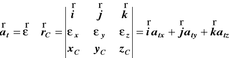
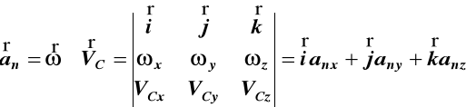
W ogólnym przypadku składowe V_C i a_C

wyznaczamy ze wzorów

(e)

(f)

(g)

W przypadku gdy oś 0z pokrywa się z osią obrotu l wtedy

ω_x = 0, ω_y = 0, ω_z =ω

ε_x = 0, ε_y = 0, ε_z = ε (h)

oraz

V_x = - ωx_C, V_y = ωx_C, V_z = 0

a_tx = - εy_C, a_ty = εx_C, a_tz = 0 (i)

a_nx = - ω²x_C, a_ny = - ω²y_C, a_nz = 0

Przy tym założeniu składowe pędu ogólnego H wynoszą

H_x = mV_Cx = - mωy_C

H_y = mV_Cy = mωx_C (j)

H_z = mV_Cz = 0

Natomiast składowe pochodnej względem czasu

pędu ogólnego H są równe

(62)

gdzie: P_x, P_y, P_z składowe sumy geometrycznej

wszystkich sił zewnętrznych działających na ciało

Równania (62) opisują zasadę pędu w ruchu obrotowym

Ogólny moment pędu (kręt) względem punktu 0 (rys.49) i (rys.50) leżącego na osi obrotu l wynosi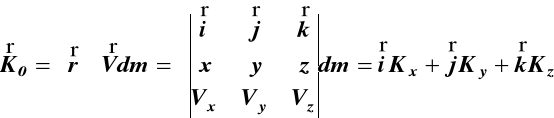

gdzie

(63)

Z wzoru (e) wynika

(k)

Podstawiając (k) do (63) i wykonując całkowanie mamy

(64)

Gdy osią obrotu jest oś 0z, wówczas wzory (64)

mają postać

K_x = - I_xzω, K_y = -I_yzω, K_z = I_zω (64)

Aby otrzymać równania dynamiczne dla ciała sztywnego

o nieruchomym jednym punkcie, oprzemy się na twierdzeniu dotyczącym krętu względem nieruchomego bieguna. Obierając jako biegun środek ruchu kulistego mamy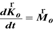
gdzie
suma momentów sił zewnętrznych (J. Misiak Mechanika Techniczna tom 2

strona 218).

Reakcje dynamiczne łożysk osi obrotu

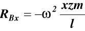
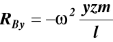
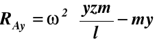
Przykład 22

Punkt materialny o masie m obraca się wokół osi AB (rys.51) z prędkością kątową ω = const.

Rozwiązanie xω²m

x l R_Bx ω

m B z

z h R_By

R_Ax z yω²m

A y

R_Ay

y Rys.51

Suma rzutów sił na osie

Suma momentów względem osi x i y

po rozwiązaniu tych równań otrzymujemy

Uwagi dotyczące wyważenia kół

ω²hm

R_A b h

0

c

h R_B

a

ω²hm

Suma rzutów sił na oś pionową

R_A - R_B - ω²hm + ω²hm = 0 stąd R_A = R_B

suma momentów względem punktu 0

dla a = b R_A = R_B = 0

50dyn

51dyn

52dyn

53dyn

54dyn

49dyn

---