Gdańsk, 04.04.2011r.
POLITECHNIKA GDAŃSKA
KATEDRA MECHANIKI BUDOWLI
I MOSTÓW
METODY DOŚWIADCZALNE
W ANALIZIE KONSTRUKCJI
Sprawozdanie: „Wyznaczanie odkształceń w belkach
zginanych (ćw. 10)”
Wykonali:
Bartosz Grzebiński
Wojciech Klimas
Grupa A1
DOŚWIADCZENIE 1 : Pomiar odkształceń w belce poddanej zginaniu prostemu .
Celem doświadczenia było pomierzenie odkształceń w przekroju α - α w belce poddanej zginaniu prostemu ( belka o przekroju dwuteowym ) .
Schemat statyczny .
15 30 15 [ cm ]
Przebieg doświadczenia :
Za pomocą tensometrów elektrooporowych , jeszcze przed obciążeniem belki , dokonano odczytów początkowych odkształceń ( OP ) . Następnie belkę obciążono zgodnie z zadanym schematem i dokonano końcowych odczytów odkształceń ( OK ).
Procedurę powtórzono trzy razy i obliczono wartości średnie przemieszczeń .
Wyniki pomiarów.
![]()
Pkt |
OP
|
OK
|
ε
|
OP
|
OK
|
ε
|
OP
|
OK
|
ε
|
ε
|
ε
|
błąd [%] |
1
|
050 |
807 |
757 |
078 |
813 |
735 |
074
|
820 |
746 |
746 |
805 |
7 |
2
|
071 |
496 |
425 |
090 |
497 |
407 |
090 |
506 |
416 |
416 |
523 |
20 |
3
|
083 |
088 |
005 |
091 |
096 |
005 |
094 |
097 |
003 |
4 |
0 |
- |
4
|
079 |
-276 |
-355 |
081 |
-276 |
-357 |
088 |
-272 |
-357 |
-357 |
-523 |
32 |
5
|
093 |
-636 |
-729 |
088 |
-632 |
-720 |
097 |
-632 |
-726 |
-726 |
-805 |
9 |
Obliczenia teoretyczne :
Moment w przekroju α - α .
Mx = - 49,05 15 = - 735,75 Ncm
E = 290000 N/cm![]()
Wymiary w [ cm ]
σ T1 = - 735,75 / 6.298 x (-2.0) = 233.660 N/cm![]()
εT1 = 2.382 / 290000 = 805x10-6
σT2 = -0.75 / 6.298 x (-1.3) = 1.548 N/cm![]()
εT2 = 1.548 / 290000 = 523x10-6
σT3 = -0.75 / 6.298 x 0.0 = 0.0 N/cm![]()
εT3 = 0.0 / 2900 = 0.0
σT4 = -0.75 / 6.298 x 1.3 = -1.548 N/cm![]()
εT4 = -1.548 / 290000 = -523x10-6
σT5 = -0.75 / 6.298 x 2.0 = -2.382 N/cm![]()
εT5 = -2.382 / 290000 = -805x10-6
DOŚWIADCZENIE 2 : Pomiar odkształceń w belce poddanej zginaniu ukośnemu .
Celem doświadczenia 2 , podobnie jak doświadczenia 1 , jest wyznaczenie przemieszczeń w belce w przekroju α - α . Należy je wykonać analogicznie jak poprzednie doświadczenie , dokonując najpierw odczytów początkowych ( OP ) - belka nieobciążona , a następnie obciążyć belkę i dokonać odczytów końcowych ( OK ).
Pomiar należy wykonać 3 razy i wyliczyć wartości średnie przemieszczeń .
15 30 15 [ cm ]
Wyniki pomiarów .
Pkt |
OP
|
OK
|
ε
|
OP
|
OK
|
ε
|
OP
|
OK
|
ε
|
ε
|
ε
|
błąd [%] |
6
|
070 |
452
|
382 |
085 |
473 |
388 |
093
|
472 |
379 |
383 |
411
|
7 |
7
|
090 |
593 |
503 |
104 |
586 |
482 |
112 |
578 |
466
|
484
|
711 |
32 |
8
|
091 |
-066 |
-156 |
095 |
-052 |
-147 |
096 |
-044 |
-140 |
-148 |
192 |
22 |
9
|
080 |
-108 |
-188 |
081 |
-115 |
-196 |
083 |
-110 |
-193 |
-192 |
-325
|
41 |
10
|
094 |
-201 |
-295 |
096 |
-218 |
-314 |
100 |
-211 |
-311 |
-307 |
-411 |
25 |
Obliczenia teoretyczne .
Wymiary [ cm ]
MX = - 19,6 15 = - 294 Ncm
MY = 0.0 Ncm
![]()
![]()
![]()
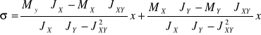
σ ( x,y ) = - 279,405x - 115,556y
σT6 = - 279,405 x 0.4 - 115,556 x (-2.0) = 119,351 N/cm![]()
εT6 = 119,351 / 290000 = 411x10-6
σ T7 = -279,405 x (-0.2) - 115,556 x (-1.3) = 206,105 N/cm![]()
εT7 = 206,105 / 290000 = 711x10-6
σ T8 = - 279,405 x (-0.2) - 115,556 x 0.0 = 55,881 N/cm![]()
εT8 = 55,881/ 290000 = 192x10-6
σ T9 = - 279,405 x (-0.2) - 115,556 x 1.3 = - 94,342 N/cm![]()
εT9 = -94,342/ 290000 = -325x10-6
σ T10 = - 279,405 x (-0.4) - 115,556 x 2.0 = - 119,351 N/cm![]()
εT10 = - 119,351 / 290000 = - 411x10-6
49,05 N
49,05 N
α
α
![]()
![]()
![]()
![]()
![]()
![]()
![]()
![]()
![]()
![]()
0,8
0,4
0,8
2,0
0,4
0,4
3,2
X
Y
T1
T2
T3
T4
T5
α
α
19,6 N
19,6 N
![]()
![]()
![]()
![]()
![]()
![]()
![]()
![]()
![]()
![]()
0,8
0,4
0,8
Y′
Y
X
X′
0,4
0,4
3,2
Wyszukiwarka