POLITECHNIKA ŚWIĘTOKRZYSKA

WYDZIAŁ BUDOWNICTWA LĄDOWEGO

KATEDRA DRÓG I MOSTÓW

KONSTRUKCJE NAWIERZCHNI DROGOWYCH

ĆWICZENIE NR 3

Projektowanie grubości płyty metodami: Westergarda, OSŻD.

GRZEGORZ SARNECKI

Grupa 32

ROK AKADEMICKI 1999/2000

I Metoda Westergaarda.

Schemat obciążenia płyty betonowej

a₁ 2a

a₁ =

Płyta z betonu cementowego 15 cm

E₁ Grunt stabilizowany asfaltem 10 cm

E₀ Piaski gruboziarniste

Dane:

Ps= 59 kN	Beton B50	Grunt stab. asfaltem	Piaski gruboziarniste
a = 17,0 cm	Rb^G = 50 MPa	E1=200 MPa	E0 = Egr = 45,0 MPa
	Eb = 39,0 GPa		μ0 = μgr = 0,20
	μb = 0,1666		μ0^2 = μgr^2 = 0,04
	μb^2 = 0,0278
	= 4,54 MPa

1. Obliczanie naprężeń.

1.1. Sprawdzenie warunku
przy h = 15cm

25,86 cm > 17,0 cm

warunek został spełniony

b =
−

b =
−
= 16,09cm

1.2. Obliczanie wartości liczbowej współczynnika reakcji podłoża k.

D = 2a = 34

 ,

wartość odczytana z nomogramu

Pa

k =


d = 2a = 34cm

k =
 , MPa

1.3. Obliczanie wartości promienia l.

l =

l =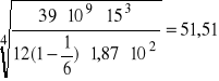
cm

1.4. Obliczenie wartości naprężenia σ_n w narożu płyty.

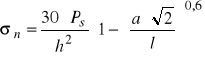
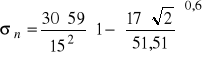
= 2,87 MPa

zaś procent wykorzystania naprężeń wynosi

P_n =
= 63,21%

1.5. Obliczenie wartości naprężenia σ_k na krawędzi płyty.

σ_k =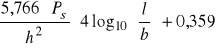

σ_k =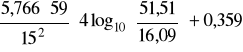
= 3,60 MPa

zaś procent wykorzystania naprężeń wynosi

P_k =
= 80,90%

1.6. Obliczenie wartości naprężenia σ_śr w środku płyty.

_śr =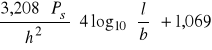

_śr =
= 2,60 MPa

zaś procent wykorzystania naprężeń wynosi

P_śr =
= 58,43%

2. Zestawienie wyników.

σ_n 2,87 Mpa

σ_{k ≤} σ^b_dop ⇒ 3,60 MPa < 4,54 MPa

σ_śr 2,60 MPa

Płyta została zaprojektowana poprawnie.

II Metoda OSŻD

Schemat obciążenia płyty betonowej

a₁ 2a

a₁ =

płyta z betonu cementowego 20 cm

E₂ grunt stabilizowany asfaltem 8 cm

E₁ bruk 10 cm

E₀ piasek gruboziarnisty

Dane:

Pn = 59 kN	Beton B50	Grunt stab. asfaltem	Bruk	Piaski gruboziarniste
Pk = 59 kN	Rb^G = 50 MPa	E2=200 MPa	E1=170 MPa	E0 = Egr = 45,0 MPa
Pśr = 59 kN	Eb = 39,0 GPa			μ0 = μgr = 0,20
an=17,0 cm	μb = 0,1666			μ0^2 = μgr^2 = 0,04
ak=17,0 cm	μb^2 = 0,0278
aśr=17,0 cm	= 4,54 MPa

1. Obliczanie naprężeń.

1.2. Sprawdzenie warunku
przy h = 20cm

34,48 cm > 17,0 cm

warunek został spełniony

b =
−

b =
−
= 15,87cm

1.3. Obliczanie wartości liczbowej współczynnika reakcji podłoża k.

D = 2a = 34

 ,

wartość odczytana z nomogramu

Pa

 ,

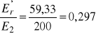
wartość odczytana z nomogramu

Pa

k =


d = 2a = 34cm

k =
 , MPa

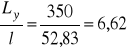
1.4. Obliczanie wartości promienia l.

l =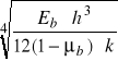

l =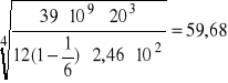
cm

1.5. Obliczenie wartości naprężenia σ_nr w narożu płyty.

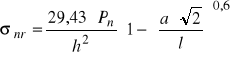
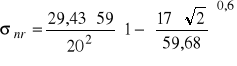
= 1,82 MPa

1.6. Obliczenie wartości naprężenia σ_kr na krawędzi płyty.

σ_kr =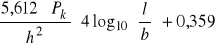

σ_kr =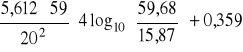
= 2,20 MPa

1.7. Obliczenie wartości naprężenia σ_śrr w środku płyty.

_śrr =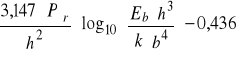

_śr =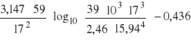
= 1,70 MPa

1.8. Obliczanie wartości naprężeń od różnicy temperatur powierzchni płyty

1.8.1. Dla naroża płyty.

E_bt = 28000 MPa

= 0,90 MPa

1.8.2 Dla krawędzi płyty.

Dla L_x = 2,5m oraz L_y = 3,5m

C_x = 0,66

C_y = 0,99

= 1,65 MPa

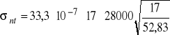
1.8.3. Dla środka płyty.

= 2,83 MPa

1.9. Obliczenie wartości maksymalnych naprężeń pochodzących od obciążenia ruchem oraz różnicy temperatur.

Przyjęto α = 1,0 −szczeliny dylatacyjne bez połączeń na rygle

β = 0,8 −nawierzchnie ze szczelinami dylatacyjnymi o odległości między nimi <80m

Wartości maksymalne (ostateczne naprężenia)

Naroże płyty
= 2,98 MPa

Krawędź płyty
= 4,12 Mpa < 4,54 MPa

Środek płyty
= 3,96 MPa

Płyta została zaprojektowana prawidłowo.

2a

2a

a

2a

2a

a

---