
Journal of Artificial Intelligence Research 18 (2003) 183-215 Submitted 9/01; published 2/03
©2003 AI Access Foundation and Morgan Kaufmann Publishers. All rights reserved.
An Evolutionary Algorithm with Advanced Goal and Priority
Specification for Multi-objective Optimization
Kay Chen Tan
ELETANKC@NUS.EDU.SG
Eik Fun Khor
EIKFUN.KHOR@SEAGATE.COM
Tong Heng Lee
ELELEETH@NUS.EDU.SG
Ramasubramanian Sathikannan
K.SATHI@GSK.COM
National University of Singapore
4 Engineering Drive 3, Singapore 117576
Republic of Singapore
Abstract
This paper presents an evolutionary algorithm with a new goal-sequence domination scheme for
better decision support in multi-objective optimization. The approach allows the inclusion of
advanced hard/soft priority and constraint information on each objective component, and is capable
of incorporating multiple specifications with overlapping or non-overlapping objective functions via
logical “OR” and “AND” connectives to drive the search towards multiple regions of trade-off. In
addition, we propose a dynamic sharing scheme that is simple and adaptively estimated according to
the on-line population distribution without needing any a priori parameter setting. Each feature in the
proposed algorithm is examined to show its respective contribution, and the performance of the
algorithm is compared with other evolutionary optimization methods. It is shown that the proposed
algorithm has performed well in the diversity of evolutionary search and uniform distribution of
non-dominated individuals along the final trade-offs, without significant computational effort. The
algorithm is also applied to the design optimization of a practical servo control system for hard disk
drives with a single voice-coil-motor actuator. Results of the evolutionary designed servo control
system show a superior closed-loop performance compared to classical PID or RPT approaches.
1. Introduction
Many real-world design tasks involve optimizing a vector of objective functions on a feasible
decision variable space. These objective functions are often non-commensurable and in
competition with each other, and cannot be simply aggregated into a scalar function for
optimization. This type of problem is known as multi-objective (MO) optimization problem, for
which the solution is a family of points known as a Pareto-optimal set (Goldberg, 1989), where
each objective component of any member in the set can only be improved by degrading at least one
of its other objective components. To obtain a good solution via conventional MO optimization
techniques such as the methods of inequalities, goal attainment or weighted sum approach, a
continuous cost function and/or a set of precise settings of weights or goals are required, which are
usually not well manageable or understood (Grace, 1992; Osyczka, 1984).
Emulating the Darwinian-Wallace principle of “survival-of-the-fittest” in natural selection and
genetics, evolutionary algorithms (EAs) (Holland, 1975) have been found to be effective and
efficient in solving complex problems where conventional optimization tools fail to work well.

T
AN
,
K
HOR
,
L
EE
,
&
S
ATHIKANNAN
184
The EAs evaluate performances of candidate solutions at multiple points simultaneously, and are
capable of approaching the global optimum in a noisy, poorly understood and/or non-differentiable
search space (Goldberg, 1989).
Since Schaffer’s work (1985), evolutionary algorithm-based search techniques for MO
optimization have been gaining significant attention from researchers in various disciplines. This
is reflected by the high volume of publications in this topic in the last few years as well as the first
international conference on Evolutionary Multi-criteria Optimization (EMO’01) held in March
2001 at Zurich, Switzerland. Readers may refer to (Coello Coello, 1996; 1999; Deb, 2001;
Fonseca, 1995; Van Veldhuizen & Lamont, 1998; Zitzler & Thiele, 1999) on detailed
implementation of various evolutionary techniques for MO optimization.
Unlike most conventional methods that linearly combine multiple attributes to form a composite
scalar objective function, the concept of Pareto's optimality or modified selection scheme is
incorporated in an evolutionary MO optimization to evolve a family of solutions at multiple points
along the trade-off surface simultaneously (Fonseca & Fleming, 1993). Among various selection
techniques for evolutionary MO optimization, the Pareto-dominance scheme (Goldberg, 1989)
that assigns equal rank to all non-dominated individuals is an effective approach for comparing the
strengths among different candidate solutions in a population (Fonseca & Fleming, 1993). Starting
from this principle, Fonseca and Fleming (1993) proposed a Pareto-based ranking scheme to
include goal and priority information for MO optimization. The underlying reason is that certain
user knowledge may be available for an optimization problem, such as preferences and/or goals to
be achieved for certain objective components. This information could be useful and incorporated
by means of goal and priority vectors, which simplify the optimization process and allow the
evolution to be directed towards certain concentrated regions of the trade-offs. Although the
ranking scheme is a good approach, it only works for a single goal and priority vector setting,
which may be difficult to define accurately prior to an optimization process for real-world
optimization problems. Moreover, the scheme does not allow advanced specifications, such as
logical “AND” and “OR” operations among multiple goals and priorities.
Based on the Pareto-based domination approach, this paper reformulates the domination scheme
to incorporate advanced specifications for better decision support in MO optimization. Besides the
flexibility of incorporating goal and priority information on each objective component, the
proposed domination scheme allows the inclusion of hard/soft priority and constraint
specifications. In addition, the approach is capable of incorporating multiple specifications with
overlapping or non-overlapping objective functions via logical “OR” and “AND” connectives to
drive the search towards multiple regions of the trade-off. The paper also proposes a dynamic
sharing scheme, which computes the sharing distance adaptively based upon the on-line
population distribution in the objective domain without the need of any a priori parameter setting.
The dynamic sharing approach is essential since it eliminates the difficulty of manually finding an
appropriate sharing distance prior to an optimization process. The choice of such a distance would
be sensitive to the size and geometry of the discovered trade-offs (Coello Coello, 1999; Fonseca &
Fleming, 1993).
This paper is organized as follows: The formulation of the proposed domination scheme for
better decision support is presented in Section 2. A dynamic sharing scheme that estimates the

A
N
E
VOLUTIONARY
A
LGORITHM FOR
M
ULTI
-
OBJECTIVE
O
PTIMIZATION
185
sharing distance adaptively based upon the on-line population distribution is described in Section 3.
Section 4 examines the usefulness and contribution of each proposed feature in the algorithm. The
performance comparison of the proposed algorithm with other evolutionary MO optimization
methods is also shown in the section. Practical application of the proposed algorithm to servo
control system design optimization is given in Section 5. Conclusions are drawn in Section 6.
2. Advanced Goal and Priority Specifications for MO Optimization
A multi-objective optimization problem seeks to optimize a vector of non-commensurable and
often competing objectives, i.e., it tends to find a parameter set P for
)
(
Min
P
F
P
Φ
∈
,
n
R
∈
P
, where
P
= {p
1
, p
2
,…, p
n
} is a n-dimensional vector having n decision variables or parameters, and
Φ
defines
a feasible set of
P. F = {f
1
, f
2
,…, f
m
} is an objective vector with m objectives to be minimized. For
a MO optimization problem with simple goal or priority specification on each objective function,
the Pareto-based ranking scheme is sufficient (Fonseca & Fleming, 1993). In practice, however, it
may be difficult to define an accurate goal and priority setting in a priori to an optimization process
for real-world optimization problems. Besides goal and priority information, there could also be
additional supporting specifications that are useful or need to be satisfied in the evolutionary search,
such as optimization constraints or feasibility of a solution. Moreover, the Pareto-based ranking
scheme does not allow advanced specifications, such as logical “AND” and “OR” operations
among multiple goals and priorities for better decision support in complex MO optimization. In
this section, a new goal-sequence Pareto-based domination scheme is proposed to address these
issues and to provide hard/soft goal and priority specifications for better controls in the
evolutionary optimization process.
2.1 Pareto-based Domination with Goal Information
This section is about an effective two-stage Pareto-based domination scheme for MO optimization,
which is then extended to incorporate advanced soft/hard goal and priority specifications. Consider
a minimization problem. An objective vector
F
a
is said to dominate another objective vector
F
b
based on the idea of Pareto dominance, denoted by
F
a
π
F
b
, iff
}
,...,
2
,
1
{
,
,
m
i
f
f
i
b
i
a
∈
∀
≤
and
j
b
j
a
f
f
,
,
<
for some
}
,...,
2
,
1
{
m
j
∈
. Adopting this basic principle of Pareto dominance, the first
stage in the proposed domination approach ranks all individuals that satisfy the goal setting to
minimize the objective functions as much as possible. It assigns the same smallest cost for all
non-dominated individuals, while the dominated individuals are ranked according to how many
individuals in the population dominate them. The second stage ranks the remaining individuals that
do not meet the goal setting based upon the following extended domination scheme. Let
a
a
)
F and
a
b
)
F denote the component of vector
a
F and
b
F respectively, in which
a
F does not meet the

T
AN
,
K
HOR
,
L
EE
,
&
S
ATHIKANNAN
186
goal
G . Then for both
a
F and
b
F that do not totally satisfy the goal
G , the vector
a
F is said
to dominate vector
b
F (denoted by
a
F
G
π
b
F ) iff
(
a
a
)
F
π
a
b
)
F ) or (abs(
a
F -G)
π
abs
(
b
F -G)) (1)
For this, the rank begins from one increment of the maximum rank value obtained in the first
stage of the cost assignment. Therefore individuals that do not meet the goal will be directed toward
the goal and the infinum in the objective domain, while those that have satisfied the goal will only
be directed further towards the infinum. Note that the domination comparison operator is
non-commutative (
a
F
G
π
b
F
≠
b
F
G
π
a
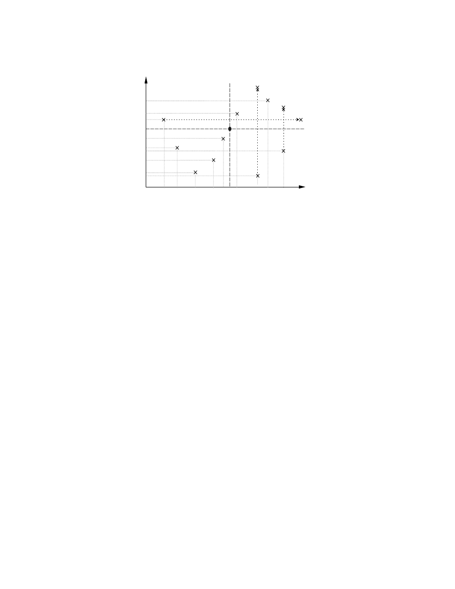
F ). Figure 1 shows an optimization problem with two
objectives f
1
and f
2
to be minimized. The arrows in Figure 1 indicate the transformation according
to
G
F
F'
−
=
of the objective function
F to F' for individuals that do not satisfy the goal, with
the goal as the new reference point in the transformed objective domain. It is obvious that the
domination scheme is simple and efficient for comparing the strengths among partially or totally
unsatisfactory individuals in a population. For comparisons among totally satisfactory individuals,
the basic Pareto-dominance is sufficient.
To study the computational efficiency in the approach, the population is divided into two
separate groups classified by the goal satisfaction, and the domination comparison is performed
separately in each group of individuals. The total number of domination comparisons for the
two-stage domination scheme is N
c
= [
G
n
(
(
G
n
(
-1)+
G
n
)
(
G
n
)
-1)] where
G
n
(
is the number of
individuals that completely satisfy the goal
G and
G
n
)
is the number of individuals partially satisfy
or completely not satisfy the goal
G. Note that
G
n
(
+
G
n
)
= N for a population size of N. Hence, in
any generation, N
c
is always less than or equal to the total number of domination comparisons
among all individuals in a population (each individual in the population is compared with (N-1)
individuals), i.e., N
c
≤
N
nc
=
)
1
(
−
N
N
. In the next section, the two-stage Pareto-based
domination scheme will be extended to incorporate soft/hard priority specifications for advanced
MO optimization.
A
N
E
VOLUTIONARY
A
LGORITHM FOR
M
ULTI
-
OBJECTIVE
O
PTIMIZATION
187
1
1
5
6
2
4
5
6
f
1
f
2
G
6
5’
6’
6’
Figure 1: Advanced Pareto Domination Scheme with Goal Information
2.2 Goal-Sequence Domination Scheme with Soft/Hard Priority Specifications
One of the advanced capabilities in evolutionary MO optimization is to incorporate cognitive
specification, such as priority information that indicates the relative importance of the multiple
tasks to provide useful guidance in the optimization. Consider a problem with multiple
non-commensurable tasks, where each task is assigned a qualitative form of priority indicating its
relative importance. In general, there exist two alternatives to accomplish these tasks, i.e., to
consider one task at a time in a sequence according to the task priority or to accomplish all tasks at
once before considering any individual task according to the task priority. Intuitively, the former
approach provides good optimization performance for tasks with higher priority and may result in
relatively poor performance for others. This is due to the fact that optimizing the higher priority
tasks may be at the performance expense of the lower priority tasks. This definition of priority is
denoted as “hard” priority in this paper. On the other hand, the latter approach provides a
distributed approach in which all tasks aim at a compromise solution before the importance or
priority of individual task is considered. This is defined as "soft" priority. Similarly, priorities for
different objective components in MO optimization can be classified as "hard" or "soft" priority.
With hard priorities, goal settings (if applicable) for higher priority objective components must be
satisfied first before attaining goals with lower priority. In contrast, soft priorities will first optimize
the overall performance of all objective components, as much as possible, before attaining any goal
setting of an individual objective component in a sequence according to the priority vector.
To achieve greater flexibility in MO optimization, the two-stage Pareto-based domination
scheme is further extended to incorporate both soft and hard priority specifications with or without
goal information by means of a new goal-sequence domination. Here, instead of having one priority
vector to indicate priorities among the multiple objective components (Fonseca & Fleming, 1998),
two kinds of priority vectors are used to accommodate the soft/hard priority information. Consider
an objective priority vector,
P
f
∈
ℵ
1xm
and a goal priority vector,
P
g
∈
ℵ
1xm
, where
P
f
(i) represents
the priority for the i
th
objective component
F(i) that is to be minimized; P
g
(i) denotes the priority for

T
AN
,
K
HOR
,
L
EE
,
&
S
ATHIKANNAN
188
the i
th
goal component
G(i) that is to be attained; m is the number of objectives to be minimized and
ℵ
denotes the natural numbers. The elements of the vector
P
f
and P
g
can take any value in the
natural numbers, with a lower number representing a higher priority and zero representing a “don’t
care” priority assignment. Note that repeated values among the elements in
P
f
and P
g
can be used to
indicate equal priority provided that
P
f
(i)
≠ P
g
(i)
∀ i ∈ {1, 2, …, m}, avoiding contradiction of the
priority assignment. With the combination of an objective priority vector
P
f
and a goal priority
vector
P
g
, soft and hard priorities can be defined provided that there is more than one preference
among the objective components as given by
∃ {(P
f
:
P
f
(j) > 1)
∨
(
P
g
:
P
g
(j) > 1)} for some j
∈ {1, 2, …, m} (2)
Based on this, a priority setting is regarded as “soft” iff
∀ i ∈ {1, 2, …, m} ∃ {(P
f
:
P
f
(i) = 1)
∨
(
P
g
:
P
g
(i) = 1)}
(3)
else, the priority is denoted as “hard”.
For example, the settings of
P
f
= [1, 1, 2, 2] and
P
g
= [0, 0, 0, 0] for a 4-objective optimization
problem indicate that the first and second objective components are given top priority to be
minimized, as much as possible, before considering minimization of the third and fourth objective
components. Since all elements in
P
g
are zeros (don’t care), no goal components will be considered
in the minimization in this case. On the other hand, the setting of
P
f
= [0, 0, 0, 0] and
P
g
= [1, 1, 2, 2]
imply that the first and second objective components are given the first priority to meet their
respective goal components before considering the goal attainment for the third and fourth
objective components. The above two different priority settings are all categorized as hard
priorities since in both cases, objective components with higher priority are minimized before
considering objective components with lower priority. For soft priority as defined in Eq. 3, the
objective priority vector and goal priority vector can be set as
P
g
= [1, 1, 1, 1] and
P
f
= [2, 2, 3, 3],
respectively. This implies that the evolution is directed towards minimizing all of the objective
components to the goal region before any attempt to minimize the higher priority objective
components in a sequence defined by the priority vector.
To systematically rank all individuals in a population to incorporate the soft/hard priority
specifications, a sequence of goals corresponding to the priority information can be generated and
represented by a goal-sequence matrix
G’ where the k
th
row in the matrix represents the goal vector
for the corresponding k
th
priority. The number of goal vectors to be generated depends on the last
level of priority z, where z is the maximum value of any one element of
P
g
and
P
f
as given by
z
= max[
P
g
(i),
P
f
(j)]
}
,...,
2
,
1
{
,
m
j
i
∈
∀
(4)
For this, the goal vectors with k
th
priority in the goal-sequence matrix
G’
k
(i) for the priority index k
= 1, 2,…, z is defined as
,
,...,
1
m
i
=
∀
G’
=
=
=
=
=
otherwise
k
i
if
k
i
if
i
i
i
i
f
g
N
j
N
j
k
)
(
)
(
)]
(
max[
)]
(
min[
)
(
)
(
,...,
1
,...,
1
P
P
F
F
G
(5)
where N denotes the population size;
)]
(
min[
,...,
1
i
N
j
=
F
and
)]
(
max[
,...,
1
i
N
j
=
F
represents the
minimum and maximum value of the i
th
objective function from the on-line population distribution,

A
N
E
VOLUTIONARY
A
LGORITHM FOR
M
ULTI
-
OBJECTIVE
O
PTIMIZATION
189
respectively. In Eq. 5, for any i
th
objective component of any k priority level, the reason for
assigning
G’
k
(i) with
G(i) is to guide the individuals towards the goal regions;
)]
(
min[
,...,
1
i
N
j
=
F
is
to minimize the corresponding objective component as much as possible; and
)]
(
max[
,...,
1
i
N
j
=
F
is
to relax the requirements on the individuals to give other objective components more room for
improvement. According to Eq. 5, the goal-sequence matrix
G’
k
(i) is dynamic at each generation, as
the values of
)]
(
min[
,...,
1
i
N
j
=
F
and
)]
(
max[
,...,
1
i
N
j
=
F
are dynamically computed depending on the
on-line population distribution. After computing the sequence of goals
G’
k
∀ k ∈ {1, 2,…, z}, the
individuals are first ranked according to the computed goal
G’
1
for the first priority. Then each
group of individuals that has the same ranks will be further compared and ranked according to next
goal
G’
2
for the second priority to further evaluate the individuals' domination in a population. In
general, this ranking process continues until there is no individual with the same rank value or after
ranking the goal
G’
z
that has the lowest priority in the goal-sequence matrix. Note that individuals
with the same rank value will not be further evaluated for those components with “don’t care”
assignments.
With the proposed goal-sequence domination scheme as given in Eq. 5, both hard and soft
priority specifications can be incorporated in MO optimization. Without loss of generality, consider
a two-objective optimization problem, with f
1
having a higher priority than f
2
, as well as a goal
setting of
G = [g
1
, g
2
]. For soft priority optimization as defined in Eq. 3, the goal priority vector and
objective priority vector can be set as
P
g
= [1, 1] and P
f
= [2, 0], respectively. Let min[F(i)] and
max[
F(i)] denote the minimum and maximum value of the i-objective component of F in a
population, respectively. The relevant goals in the goal-sequence matrix for each priority level as
defined in Eq. 5 are then given as
G’
1
=
G for the first priority and G’
2
= {min[
F(1)], max[F(2)]}
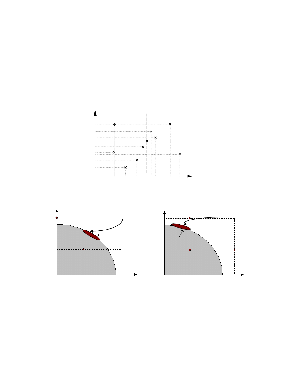
for the second priority. The goal-sequence domination scheme for the two-objective minimization
problem is illustrated in Figure 2. Here, the rank value of each individual is denoted by r
1
→ r
2
,
where r
1
and r
2
is the rank value after the goal-sequence ranking of the first and second priority,
respectively. The preference setting indicates that both g
1
and g
2
are given the same priority to be
attained in the optimization before individuals are further ranked according to the higher priority of
f
1
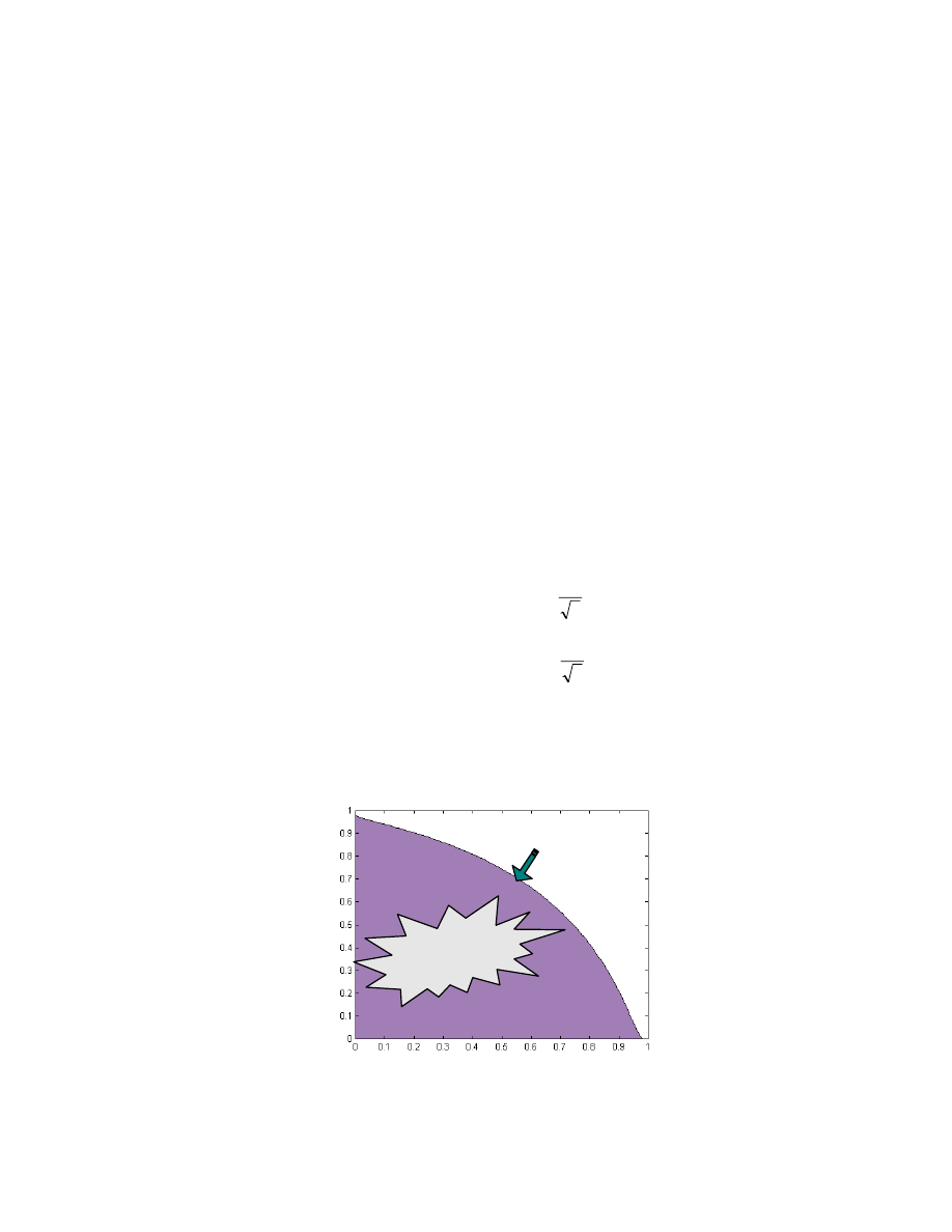
. This is illustrated in Figure 3a, which shows the location of the desired Pareto-front (represented
by the dark region) and the expected evolution direction (represented by the curved arrow) in the
objective domain for an example with an unfeasible goal setting
G.
For hard priority optimization as defined in Eqs. 2 and 3, the goal priority vector and objective
priority vector can be set as
P
g
= [1, 2] and
P
f
= [0, 0], respectively. According to Eq. 5, this gives a
goal sequence of
G’
1
= [g
1
, max[
F(2)] and G’
2
= [max[
F(1)], g
2
] for the first and second priority,
respectively. It implies that g
1
is given higher priority than g
2
to be attained in the optimization.
Figure 3b shows the location of the desired Pareto-front (represented by dark region) and the
expected evolution direction (represented by curved arrow) in the objective domain. As compared
to the solutions obtained in soft priority optimization, hard priority optimization attempts to attain
the first goal component and leads to the solution with better f
1
(higher priority) but worse f
2
(lower
priority). It should be mentioned that the setting of soft/hard priority may be subjective or problem
T
AN
,
K
HOR
,
L
EE
,
&
S
ATHIKANNAN
190
dependent in practice. In general, the hard priority optimization may be appropriate for problems
with well-defined goals in order to avoid stagnation with unfeasible goal settings. Soft priority
optimization is more suitable for applications where moderate performance among various
objective components is desired. Besides soft/hard priority information, there may be additional
specifications such as optimization constraints that are required to be satisfied in the optimization.
These specifications could be easily incorporated in MO optimization by formulating the
constraints as additional objective components to be optimized (Fonseca & Fleming, 1998). This
will be discussed in the next section.
1
→
2
1
→
1
5
→
6
2
→
3
4
→
4
5
→
5
7
→
8
f
1
f
2
7
→
7
G'
2
g
1
g
2
G'
1
Figure 2: Goal-sequence Domination with Goal
G = {g
1
, g
2
}, Priority
P
g
= [1, 1] and P
f
= [2, 0]
f
1
G
f
2
Unfeasible
Region
desired solution
Evolutio
n
Evolutio
n
g
1
g
2
G
G
1
2
'
'
(a) Soft priority f
1
higher than f
2
f
1
f
2
G
Unfeasible
Region
Evolutio
n
desired solution
g
1
g
2
G'
2
G'
1
max[F(1)]
max[F(2)]
(b) Hard priority f
1
higher than f
2
Figure 3: Illustration of Soft and Hard Priority with Unfeasible Goal Setting
2.3 Optimization with Soft and Hard Constraints
Constraints often exist in practical optimization problems (Luus et al. 1995; Michalewicz &
Schoenauer, 1996). These constraints are often incorporated in the MO optimization function as

A
N
E
VOLUTIONARY
A
LGORITHM FOR
M
ULTI
-
OBJECTIVE
O
PTIMIZATION
191
one of the objective components to be optimized. It could be in the form of "hard" constraint where
the optimization is directed towards attaining a threshold or goal, and further optimization is
meaningless or not desirable whenever the goal has been satisfied. In contrast, a "soft" constraint
requires that the value of objective component corresponding to the constraint is optimized as much
as possible. An easy approach to deal with both hard and soft constraints concurrently in
evolutionary MO optimization is given here. At each generation, an updated objective function
F
x
#
concerning both hard and soft constraints for an individual x with its objective function
F
x
can be
computed in a priori to the goal-sequence domination scheme as given by
[
] [
]
<
=
otherwise
i
i
i
if
i
i
i
)
(
)
(
&
hard
is
)
(
)
(
)
(
)
(
#
G
F
G
F
G
F
x
x
x
}
,...,
1
{
m
i
=
∀
(6)
In Eq. 6, any objective component i that corresponds to a hard constraint is assigned to the value
of
G(i) whenever the hard constraint has been satisfied. The underlying reason is that there is no
ranking preference for any particular objective component that has the same value in an
evolutionary optimization process, and thus the evolution will only be directed towards optimizing
soft constraints and any unattained hard constraints, as desired.
2.4 Logical Connectives among Goal and Priority Specifications
For MO optimization problems with a single goal or priority specification, the decision maker often
needs to “guess” an appropriate initial goal or priority vector and then manually observe the
optimization progress. If any of the goal components is too stringent or too generous, the goal
setting will have to be adjusted accordingly until a satisfactory solution can be obtained. This
approach obviously requires extensive human observation and intervention, which can be tedious
or inefficient in practice. Marcu (1997) proposed a method of adapting the goal values based upon
the on-line population distribution at every generation. However, the adaptation of goal values is
formulated in such a way that the search is always uniformly directed towards the middle region of
the trade-offs. This restriction may be undesirable for many applications, where the trade-off
surface is unknown or the search needs to be directed in any direction other than the middle region
of the trade-off surface. To reduce human interaction and to allow multiple sets of goal and priority
specifications that direct the evolutionary search towards a different portion of the trade-off surface
in a single run, the goal-sequence domination scheme is extended in this section to enable logical
statements such as “OR” (
∪ ) and “AND” ( ∩ ) operations among multiple goal and priority
specifications.
These logical operations can be built on top of the goal-sequence domination procedure for each
specification. By doing this, the unified rank value for each individual can be determined and taken
into effect immediately in the evolution towards the regions concerned. Consider ranking an
objective vector
F
x
by comparing it to the rest of the individuals in a population with reference to
two different specification settings of
S
i
and
S
j
, where
S
i
and
S
j
are the specifications concerning
any set of objective functions with or without goals and priorities. Let these ranks be denoted by
rank(
F
x
,
S
i
) and rank(
F
x
,
S
j
), respectively. The “OR” and “AND” operations for the two goal
settings are then defined as,

T
AN
,
K
HOR
,
L
EE
,
&
S
ATHIKANNAN
192
{
}
)
,
(
),
,
(
min
)
,
(
j
x
i
x
j
i
x
rank
rank
rank
S
S
S
S
F
F
F
=
∪
(7a)
{
}
)
,
(
),
,
(
max
)
,
(
j
x
i
x
j
i
x
rank
rank
rank
S
S
S
S
F
F
F
=
∩
(7b)
According to Eq. 7, the rank value of vector
F
x
for an “OR” operation between any two
specifications
S
i
and
S
j
takes the minimum rank value with respect to the two specification settings.
This is in order to evolve the population towards one of the specifications in which the objective
vector is less strongly violated. In contrast, an “AND” operation takes the maximum rank value in
order to direct the evolutionary search towards minimizing the amount of violation from both of the
specifications concurrently. Clearly, the “AND” and “OR” operations in Eq. 7 can be easily
extended to include general logical specifications with more complex connectives, such as “(
S
i
OR
S
j
) AND (
S
k
OR
S
l
)”, if desired.
3. Dynamic Sharing Scheme and MOEA Program Flowchart
3.1 Dynamic Sharing Scheme
Fitness sharing was proposed by Goldberg and Richardson (1987) to evolve an equally distributed
population along the Pareto-optimal front or to distribute the population at multiple optima in the
search space. The method creates sub-divisions in the objective domain by degrading an individual
fitness upon the existence of other individuals in its neighborhood defined by a sharing distance.
The niche count,
( )
∑
=
N
j
j
i
i
d
sh
m
,
, is calculated by summing a sharing function over all members of
the population, where the distance d
i,j
represents the distance between individual i and j. The
sharing function is defined as
( )
<
−
=
otherwise
d
if
d
d
sh
share
j
i
share
i,j
j
i
0
1
,
,
σ
σ
α
(8)
with the parameter
α
being commonly set to 1.
The sharing function in Eq. 8 requires a good setting of sharing distance
σ
share
to be estimated
upon the trade-off surface, which is usually unknown in many optimization problems (Coello
Coello, 1999). Moreover, the size of objective space usually cannot be predefined, as the exact
bounds of the objective space are often undetermined. Fonseca and Fleming (1993) proposed the
method of Kernel density estimation to determine an appropriate sharing distance for MO
optimization. However, the sharing process is performed in the ‘sphere’ space which may not
reflect the actual objective space for which the population is expected to be uniformly distributed.
Miller and Shaw (1996) proposed a dynamic sharing method for which the peaks in the parameter
domain are ‘dynamically’ detected and recalculated at every generation with the sharing distance
remains predefined. However, the approach is made on the assumption that the number of niche
peaks can be estimated and the peaks are all at the minimum distance of 2
σ
share
from each other.

A
N
E
VOLUTIONARY
A
LGORITHM FOR
M
ULTI
-
OBJECTIVE
O
PTIMIZATION
193
Moreover, their formulation is defined in the parameter space to handle multi-modal function
optimization, which may not be appropriate for distributing the population uniformly along the
Pareto-optimal front in the objective domain.
In contrast to existing approaches, we propose a dynamic sharing method that adaptively
computes the sharing distance
σ
share
to uniformly distribute all individuals along the Pareto-optimal
front at each generation. This requires no prior knowledge of the trade-off surface. Intuitively, the
trade-offs for an m-objective optimization problem are in the form of an (m-1) dimensional
hyper-volume (Tan et al. 1999), which can be approximated by the hyper-volume V
pop
(n)
of a
hyper-sphere as given by,
1
)
(
2
/
)
1
(
)
(
2
!
2
1
−
−
×
−
=
m
n
m
n
pop
d
m
V
π
(9)
where
)
(n
d
is the diameter of the hyper-sphere at generation n. Note that computation of the
diameter
)
(n
d
depends on the curvature of the trade-off curve formed by the non-dominated
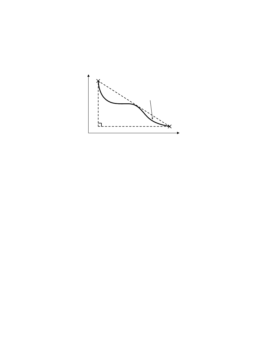
individuals in the objective space. For a two-objective optimization problem, the diameter
)
(n
d
is
equal to the interpolated distance of the trade-off curve covered by the non-dominated individuals
as shown in Figure 4. Although computation of
)
(n
d
that accurately represents the interpolated
curvature of the non-dominated individuals distribution is complex, it can be estimated by the
average distance between the shortest and the longest possible diameter given by d
min
(n)
and d
max
(n)
respectively (Tan et al. 1999). Let
F
x
and
F
y
denote the objective function of the two furthest
individuals in a population. Then d
min
(n)
is equal to the minimum length between
F
x
and
F
y
, and
d
max
(n)
can be estimated by d
1
(n)
+ d
2
(n)
as shown in Figure 4.
The same procedure can also be extended to any multi-dimensional objective space. To achieve
a uniformly distributed population along the trade-off set, the sharing distance
σ
share
(n)
could be
computed as half of the distance between each individual in the (m-1)-dimensional hyper-volume
V
pop
(n)
covered by the population size N at generation n,
(
)
)
(
1
)
(
2
/
)
1
(
!
2
1
n
pop
m
n
share
m
V
m
N
=
×
−
×
−
−
σ
π
(10)
Substituting Eq. 9 into Eq. 10 gives the sharing distance
σ
share
(n)
at generation n in term of the
diameter
)
(n
d
and the population size N as given by
2
)
(
)
1
/(
1
)
(
n
m
n
share
d
N
×
=
−
σ
(11)
Clearly, Eq. 11 provides a simple computation of
σ
share
that is capable of distributing the
population evenly along the Pareto front, without the need for any prior knowledge of the usually
T
AN
,
K
HOR
,
L
EE
,
&
S
ATHIKANNAN
194
unknown fitness landscape. Moreover, adopting the computation of sharing distance that is
dynamically based upon the population distribution at each generation is also more appropriate and
effective than the method of off-line estimation with pre-assumed trade-off surface as employed in
most existing sharing methods, since the trade-off surface may be changed any time along the
evolution whenever the goal setting is altered.
d
min
(n)
d
(n)
d
1
(n)
d
2
(n)
Discovered
trade-off curve
f
2
f
1
F
y
F
x
Figure 4: The Diameter
)
(n
d
of a Trade-off Curve
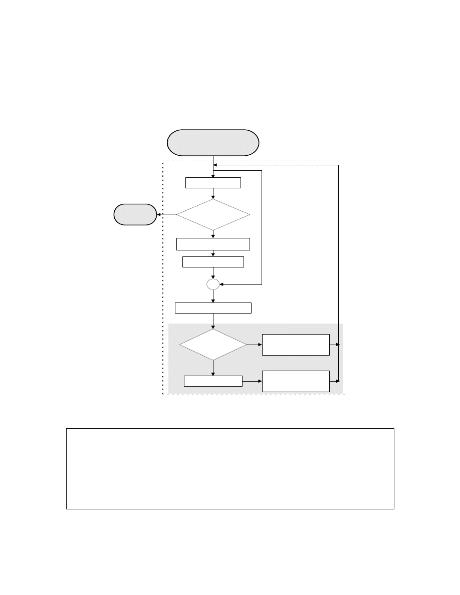
3.2 MOEA Program Flowchart
The overall program flowchart of this paper’s multi-objective evolutionary algorithm (MOEA) is
illustrated in Figure 5. At the beginning of the evolution, a population of candidate solutions is
initialized and evaluated according to a vector of objective functions. Based upon the user-defined
specifications, such as goals, constraints, priorities and logical operations, the evaluated individuals
are ranked according to the goal-sequence domination scheme (described in Section 2) in order to
evolve the search towards the global trade-off surface. The resulted rank values are then further
refined by the dynamic sharing scheme (described in Section 3.1) in order to distribute the
non-dominated individuals uniformly along the discovered Pareto-optimal front. If the stopping
criterion is not met, the individuals will undergo a series of genetic operations which are detailed
within the “genetic operations” in Figure 6. Here, simple genetic operations consisting of
tournament selection (Tan et al. 1999), simple crossover with mating restriction that selects
individuals within the sharing distance for mating (Fonseca & Fleming, 1998) as well as simple
mutation are performed to reproduce offspring for the next generation.
After the genetic operations, the newly evolved population is evaluated and combined with the
non-dominated individuals preserved from the previous generation. The combined population is
then subjected to the domination comparison scheme and pruned to the desired population size
according to the Switching Preserved Strategy (SPS) (Tan et al. 1999). This maintains a set of
stable and well-distributed non-dominated individuals along the Pareto-optimal front. In SPS, if the
number of non-dominated individuals in the combined population is less than or equal to the
desired population size, extra individuals are removed according to their rank values in order to
promote stability in the evolutionary search towards the final trade-offs. Otherwise, the
A
N
E
VOLUTIONARY
A
LGORITHM FOR
M
ULTI
-
OBJECTIVE
O
PTIMIZATION
195
non-dominated individuals with high niched count value will be discarded in order to distribute the
individuals uniformly along the discovered Pareto-optimal front. After the process, the remaining
individuals are allowed to survive in the next generation and this evolutionary cycle is repeated
until the stopping criterion is met.
Population initialization
Function evaluation
D om ination com parison
D ynamic sharing
Is
stopping criterion
m et?
G enetic operations
Function evaluation
D om ination com parison
Size(nondom )
> popsize?
D ynamic sharing
Filtering - based on
Pareto ranked cost
Filtering - based on
shared costs
Final
population
Y es
N o
Y es
N o
non-domina
te
d i
ndivi
dua
ls
ne
w popu
la
ti
on
evolved
population
Σ
com bined
population
Figure 5: Program Architecture of the MOEA
Genetic Operations for MOEA:
Let,
pop
(n)
= population in current generation n
Step 1) Perform tournament selection to select individuals from pop
(n)
. The selected population is
called selpop
(n)
.
Step 2) Perform simple crossover and mating restriction for selpop
(n)
using the dynamic sharing
distance in Step 1. The resulted population is called crosspop
(n)
.
Step 3) Perform simple mutation for crosspop
(n)
. The resulted population is called evolpop
(n)
.
Figure 6: Detailed procedure within the box of “genetic operations” in Figure 5
T
AN
,
K
HOR
,
L
EE
,
&
S
ATHIKANNAN
196
4. Validation Results on Benchmark Problems
This section validates the proposed algorithm in two ways. The first kind of validation (presented in
Section 4.1) illustrates how each of the proposed features, including goal-sequence domination
scheme, hard/soft goal and priority specifications, logical operations among multiple goals and
dynamic sharing, enhances the performance of MOEA in MO optimization. As shown in Section
4.2, the second type of validation compares performance of the proposed MOEA with various
evolutionary algorithms based upon a benchmark problem. Various performance measures are used
in the comparison and the results are then discussed.
4.1 Validation of the Proposed Features in MOEA
In this section, various proposed features in MOEA are examined for their usefulness in MO
optimization. This study adopts the simple two-objective minimization problem (Fonseca &
Fleming, 1993) that allows easy visual observation of the optimization performance. The function
has a large and non-linear trade-off curve, which challenges the algorithm’s ability to find and
maintain the entire Pareto-optimal front uniformly. The two-objective functions, f
1
and f
2
, to be
minimized are given as
∑
+
−
−
=
∑
−
−
−
=
=
=
2
8
1
8
1
2
2
8
1
8
1
1
8
1
1
)
,...,
(
8
1
1
)
,...,
(
i
i
i
i
x
exp
x
x
f
x
exp
x
x
f
(12)
where,
8
,...,
2
,
1
,
2
2
=
∀
<
≤
−
i
x
i
. The trade-off line is shown by the curve in Figure 7, where the
shaded region represents the unfeasible area in the objective domain.
f
1
f
2
Trade-off
Curve
Unfeasible
Region
Figure 7: Pareto-optimal Front in the Objective Domain
A
N
E
VOLUTIONARY
A
LGORITHM FOR
M
ULTI
-
OBJECTIVE
O
PTIMIZATION
197
The simulations are run for 70 generations with a population size of 100. Standard mutation with
a probability of 0.01 and standard two-point crossover with a probability of 0.7 are used. To study
the merit of the dynamic sharing scheme in MOEA as proposed in Section 3.1, 4 different types of
simulations have been performed. The first type is without fitness sharing. The second and third
employ a fixed sharing distance of 0.01 and 0.1, respectively. The fourth uses the dynamic sharing
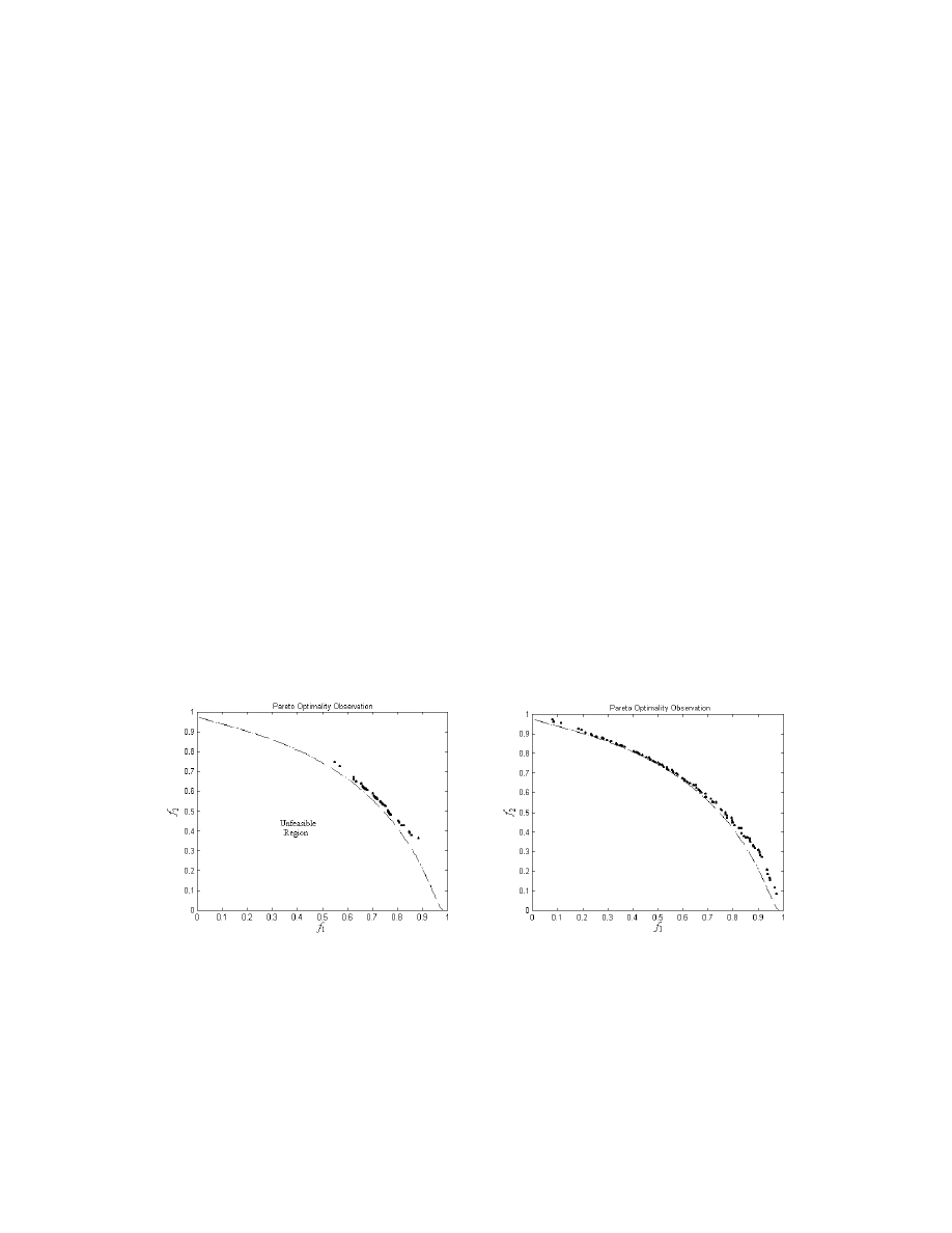
scheme which does not require any predefined sharing distance setting. Figure 8 illustrates the
respective population distribution in the objective domain at the end of the evolution. It can be
observed that all of the four simulations are able to discover the final trade-off, but with some
performance difference in terms of the closeness and uniformity of the population distribution
along the trade-off curve.
For the MOEA without fitness sharing as shown in Figure 8a, the population tends to converge
to an arbitrary part of the trade-off curve. This agrees with the findings of Fonseca and Fleming,
(1993). For the MOEA with fitness sharing, as shown in Figures 8b and 8c, the population can be
distributed along the trade-off curve rather well, although the sharing distance of 0.01 provides a
more uniform distribution than that of 0.1. This indicates that although fitness sharing contributes
to population diversity and distribution along the trade-off curve, the sharing distance has to be
chosen carefully in order to ensure the uniformity of the population distribution. This often
involves tedious trial-and-error procedures in order to ‘guess’ an appropriate sharing distance,
since it is problem dependent and based upon the size of the discovered trade-offs as well as the
number of non-dominated individuals. These difficulties can be solved with the proposed dynamic
sharing scheme, which has the ability to automatically adapt the sharing distance along the
evolution without the need of any predefined parameter, as shown in Figure 8d.
(a) No sharing
(b) Sharing distance = 0.01
T
AN
,
K
HOR
,
L
EE
,
&
S
ATHIKANNAN
198
(c) Sharing distance = 0.1
(d) Dynamic sharing
Figure 8: Performance Validation of Dynamic Sharing Scheme in MOEA
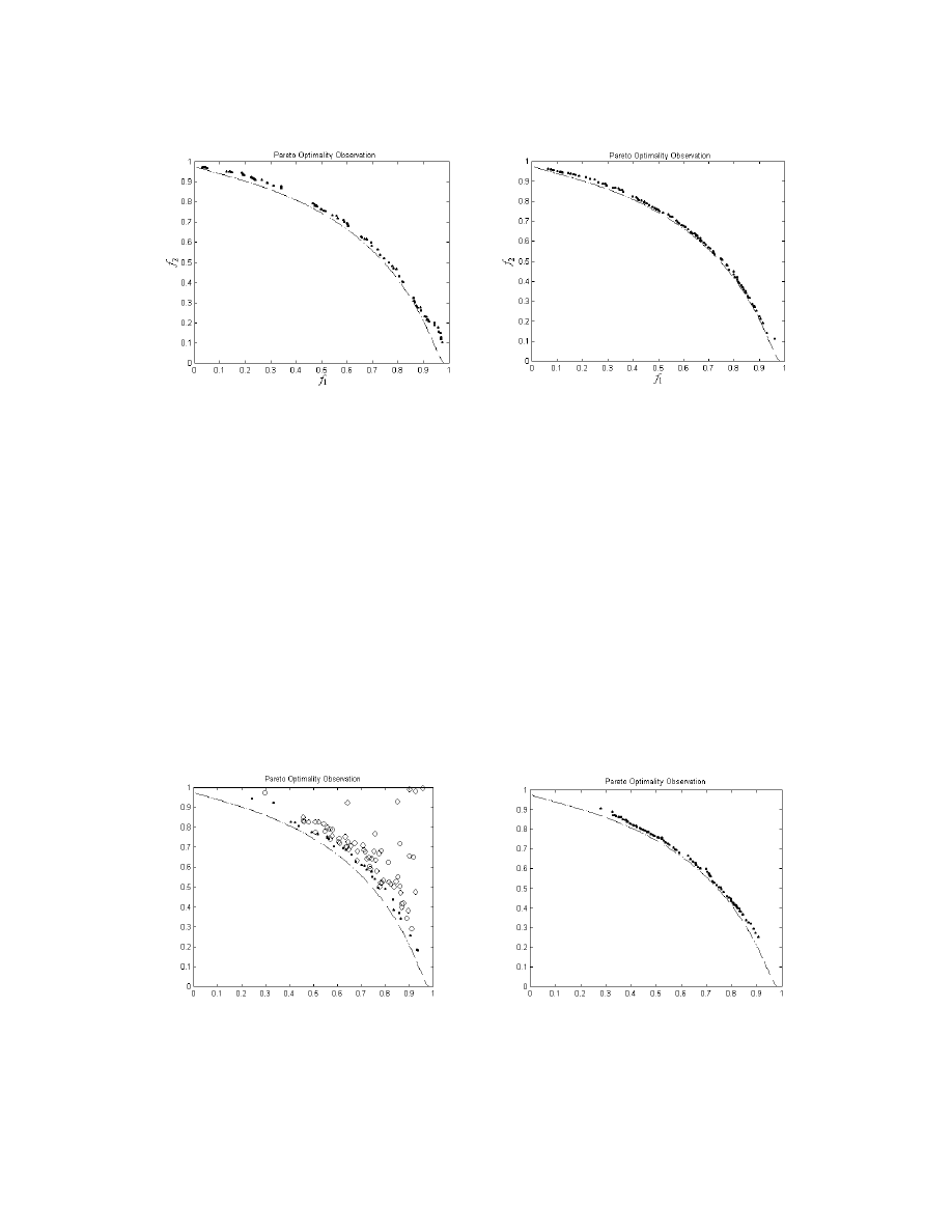
To validate the contribution of the switching preserved strategy (SPS) in MOEA, the above
simulation was repeated with different scenarios and settings. Figure 9a depicts the simulation
result without the implementation of SPS, in which the evolution faces difficulty converging to the
trade-off curve. The solid dots represent the non-dominated individuals while the empty circles
represent the dominated individuals. As can be seen, the final population is crowded and the
non-dominated individuals are distributed with some distance away from the trade-off curve.
Figure 9b shows the simulation result for the MOEA with SPS and filtering solely based upon the
Pareto domination. The final population has now managed to converge to the Pareto-optimal front.
However, the non-dominated individuals are not equally distributed and the diversity of the
population is poor: they only concentrate on a portion of the entire trade-off curve (c.f. Figures 8d,
9b). These results clearly show that SPS in MOEA is necessary in order to achieve good stability
and diversity of the population in converging towards the complete set of trade-offs.
Unfeasible
region
f
1
f
2
(a) Without SPS
f
1
f
2
Unfeasible
region
(b) With SPS solely based on Pareto ranked cost
Figure 9: Performance Validation of SPS in MOEA
A
N
E
VOLUTIONARY
A
LGORITHM FOR
M
ULTI
-
OBJECTIVE
O
PTIMIZATION
199
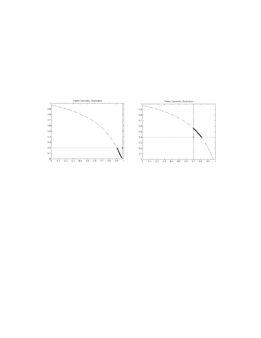
The proposed goal-sequence domination scheme was also validated for problems with different
goal settings, including a feasible but extreme goal setting of (0.98, 0.2) and an unfeasible goal
setting of (0.7, 0.4) as shown in Figures 10 and 11, respectively. As desired, the population is seen
to concentrate on the preferred region of the trade-off curve at the end of the evolution, regardless
of the unattainable or extreme goal settings. As shown in Figures 10 and 11, MOEA is capable of
uniformly distributing the non-dominated individuals along any trade-offs size resulting from
different goal settings, with the help of the dynamic sharing scheme that automatically computes a
suitable sharing distance for optimal population distribution at each generation.
f
1
f
2
f
1
f
2
Figure 10: Feasible but Extreme Goal Setting
Figure 11: Unfeasible Goal Setting
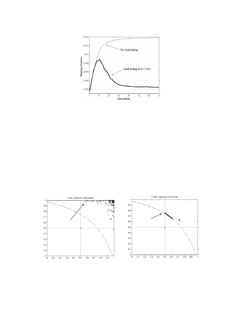
Figure 12 shows the trace of sharing distance during the evolution. The thin and thick lines
represent the average sharing distance without any goal setting (see Figure 8d for the corresponding
Pareto-front) and with the goal setting of (0.7, 0.4) (see Figure 11 for the corresponding
Pareto-front), respectively. Generally, MO optimization without a goal setting has an initially small
size of discovered Pareto-front, which subsequently grows along with the evolution to approach
and cover the entire trade-off region at the end of evolution. This behavior is explained in Figure 12
where the sharing distance increases asymptotically along the evolution until a steady value of
0.0138 is reached. It should be noted that this value is close to the fixed sharing distance of 0.01 in
Figure 8b, which was carefully chosen after trial-and-error procedures. For the case of MOEA with
a goal setting of (0.7, 0.4), the sharing distance increases initially and subsequently decreases to
0.0025 along the evolution, which is lower than the value of 0.0138 (without goal setting). The
reason is that the concentrated trade-off region within the goal setting is smaller than the entire
trade-off region (without goal setting), and hence results in a smaller distance for uniform sharing
of non-dominated individuals. These experiments show that the proposed dynamic sharing scheme
can effectively auto-adapt the sharing distance to arrive at an appropriate value for uniform
population distribution along the discovered trade-off region at different sizes, without the need for
any a priori parameter setting.
T
AN
,
K
HOR
,
L
EE
,
&
S
ATHIKANNAN
200
Figure 12: Trace of the Dynamic Sharing Distance Along the Evolution
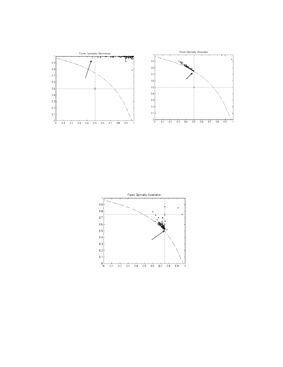
Figures 13 and 14 show the MOEA simulation results for the case of an infeasible goal setting
with soft and hard priorities, respectively. In the figures, diamonds represent goals, small circles
represent non-dominated individuals and solid dots represent dominated individuals. For the soft
priority setting in Figure 13, goals are treated as first priority followed by the objective component
of f
1
as second priority, i.e.,
P
g
= [1, 1] and
P
f
= [2, 0]. As can be seen, it provides a distributive
optimization approach for all goals by pushing the population towards the objective component of
f
1
that has a higher priority, after taking the goal vector into consideration (c.f. Figures 3a, 13b). In
contrast, Figure 14 shows the minimization results with hard priority setting where priority of f
1
is
higher than f
2
, i.e.,
P
g
= [1, 2] and
P
f
= [0, 0]. Unlike the soft priority optimization, hard priority
minimizes the objective of f
1
until the relevant goal component of g
1
= 0.5 is satisfied before
attaining the objective component of f
2
with the second goal component of g
2
= 0.5, as shown in
Figure 14 (c.f. Figures 3b, 14b). As can be seen, objective values with hard priority settings are
better with higher priority but are worse with lower priority, as compared to the solutions obtained
in soft priority optimization (c.f. Figures 13b, 14b).
Non-dominated
individual
f
1
f
2
f
1
Non-dominated
individual
f
1
f
2
(a) At generation 5
(b) At generation 70
Figure 13: MOEA Optimization with Unfeasible Goal Setting: f
1
has Soft Priority Higher than f
2
A
N
E
VOLUTIONARY
A
LGORITHM FOR
M
ULTI
-
OBJECTIVE
O
PTIMIZATION
201
Non-dominated
individual
f
1
f
2
f
1
Non-dominated
individual
f
2
f
1
(a) At generation 5
(b) At generation 70
Figure 14: MOEA Optimization with Unfeasible Goal Setting: f
1
has Hard Priority Higher than f
2
Figure 15 shows the MOEA minimization result with f
1
being a hard constraint. The population
continuously evolves towards minimizing f
2
only after the hard constraint of f
1
has been satisfied. In
general, objective components with hard constraints may be assigned as hard priorities in order to
meet the hard constraints before minimizing any other objective components.
Non-dominated
individuals
f
1
f
2
f
1
f
2
Figure 15: MOEA Minimization with Hard Constraint on f
1
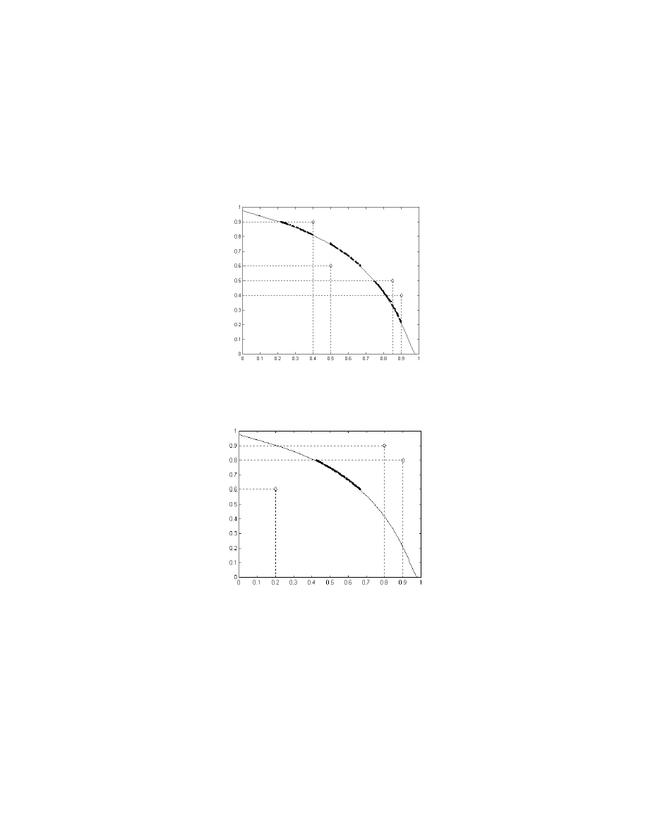
Figures 16 and 17 show the MO optimization results that include multiple goal settings specified
by logical “OR” (
∪
) and “AND” (
∩
) connectives, respectively. For the “OR” operation as shown
in Figure 16, the population is automatically distributed and equally spread over the different
concentrated trade-off regions to satisfy the goal settings separately, regardless of the overlapping
or feasibility of the goals. With the proposed dynamic sharing scheme, the sub-population size for
each goal is in general based upon the relative size of the concentrated trade-off surface of that goal,
T
AN
,
K
HOR
,
L
EE
,
&
S
ATHIKANNAN
202
and thus individuals are capable of equally distributing themselves along the different concentrated
trade-off regions. For the “AND” operation as illustrated in Figure 17, the whole population
evolves towards minimizing all the goals
G
1
,
G
2
and
G
3
simultaneously. As a result, the individuals
are equally distributed over the common concentrated trade-off surface formed by the three goals,
as desired.
G
1
G
2
G
3
G
4
Pareto optimality observation
f
1
f
2
G
1
G
2
G
3
G
4
Figure 16: MOEA Minimization for (
G
1
∪
G
2
∪
G
3
∪
G
4
)
G
1
G
2
G
3
Pareto optimality observation
f
1
f
2
G
3
G
2
G
1
Figure 17: MOEA Minimization for (
G
1
∩
G
2
∩
G
3
)
4.2 Performance Comparisons of MOEA
This section studies and compares the performance of the proposed MOEA with other
multi-objective evolutionary optimization methods based upon a benchmark MO optimization
problem. For a comprehensive comparison, various performance measures are used and the
comparison results are discussed in the section.
4.2.1 The Test Problem
A
N
E
VOLUTIONARY
A
LGORITHM FOR
M
ULTI
-
OBJECTIVE
O
PTIMIZATION
203
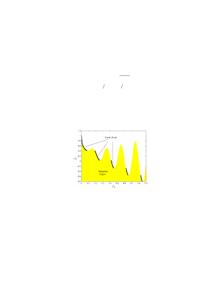
The test problem used for the performance comparisons is a two-objective minimization problem
(Deb, 1999). The problem is chosen because it has a discontinuous Pareto-front which challenges
the evolutionary algorithm’s ability to find and maintain the Pareto-optimal solutions that are
discontinuously spread in the search space. The problem involves minimizing the objective
functions f
1
and f
2
as given below,
( )
1
1
1
x
x
f
= (13a)
(
)
,
1
10
10
1
,...,
10
2
10
2
−
∑
+
=
=
i
i
x
x
x
g
(13b)
(
)
(
)
(
) (
)
1
1
25
.
0
1
1
10
sin
1
,
f
g
f
g
f
g
f
h
π
−
−
=
(13c)
( ) (
) (
)
g
f
h
x
x
g
x
f
,
,...,
1
10
2
1
2
=
(13d)
All variables are varied in [0, 1] and the true Pareto-optimal solutions are constituted with x
i
= 0
∀ i = 2, …, 10 and the discontinuous values of x
1
in the range of [0, 1] (Deb, 1999). Figure 18
depicts the discontinuous Pareto-optimal front (in bold). The shaded region represents the
unfeasible region in the search space.
Figure 18: Pareto-optimal Front in the Objective Domain
4.2.2 Current Evolutionary MO Optimization Methods
Besides MOEA, five well-known multi-objective evolutionary optimization methods are used in
the comparison. These approaches differ from each other in their working principles and
mechanisms and have been widely cited or applied to real-world applications. The algorithms are
summarized below and readers may refer to their respective references for detailed information.
(i) Fonseca and Fleming’s Genetic Algorithm (FFGA): For MO optimization, Fonseca and
Fleming (1993) proposed a multi-objective genetic algorithm (MOGA) with Pareto-based ranking
scheme, in which the rank of an individual is based on the number of other individuals in the current

T
AN
,
K
HOR
,
L
EE
,
&
S
ATHIKANNAN
204
population that dominate it. Their algorithm was further incorporated with fitness sharing and
mating restriction to distribute the population uniformly along the Pareto-optimal front.
(ii) Niched Pareto Genetic Algorithm (NPGA): The method of NPGA (Horn & Nafpliotis, 1993)
works on a Pareto-dominance-based tournament selection scheme to handle multiple objectives
simultaneously. To reduce the computational effort, a pre-specified number of individuals are
picked as a comparison set to help determine the dominance. When both competitors end in a tie,
the winner is decided through fitness sharing (Goldberg and Richardson, 1987).
(iii) Strength Pareto Evolutionary Algorithm (SPEA): The main features of SPEA (Zitzler &
Thiele, 1999) are the usage of two populations (P and P’) and clustering. In general, any
non-dominated individual is archived in P’ and any dominated individual that is dominated by
other members in P’ is removed. When the number of individuals in P’ exceeds a maximum value,
clustering is adopted to remove the extra individuals in P’. Tournament selection is then applied to
reproduce individuals from P + P’ before the evolution proceeds to the next generation.
(iv) Non-Generational Genetic Algorithm (NGGA): In NGGA (Borges & Barbosa, 2000), a cost
function of an individual is a non-linear function of domination measure and density measure on
that individual. Instead of evolving the whole population at each iteration, a pair of parents is
selected to reproduce two offsprings. An offspring will replace the worst individual in a population
if the offspring has lower cost function than the worst individual.
(v) Murata and Ishibuchi’s Genetic Algorithm (MIGA): Unlike the above evolutionary
optimization methods, MIGA (Murata & Ishibuchi, 1996) applies the method of weighted-sum to
construct the fitness of each individual in a population. To keep the diversity of the population
along the Pareto-optimal front, the weights are randomly specified when a pair of parent solutions
is selected from a current population for generating the offspring.
4.2.3 Performance Measures
This section considers three different performance measures which are complementary to each
other: Size of space covered (SSC), uniform distribution (UD) index of non-dominated individuals
and number of function evaluation (Neval).
(i) Size of Space Covered (SSC): This measure was proposed by Zitzler and Thiele (1999) as a
measure to quantify the overall size of phenotype space covered (SSC) by a population. In general,
the higher the value of SSC, the larger the space covered by the population and hence the better the
optimization result.
(ii) Uniform Distribution (UD) of Non-dominated Population: Besides the size of space covered
by a population, it is also essential to examine the ability of an evolutionary optimization to
distribute their non-dominated individuals as uniformly as possible along the discovered

A
N
E
VOLUTIONARY
A
LGORITHM FOR
M
ULTI
-
OBJECTIVE
O
PTIMIZATION
205
Pareto-optimal front, unless prohibited by the geometry of the Pareto front. This is to achieve a
smooth transition from one Pareto-optimal solution to its neighbors, thus facilitating the
decision-maker in choosing his/her final solution. Mathematically, UD(X') for a given set of
non-dominated individuals X' in a population X, where X'
⊆ X, is defined as (Tan et al. 2001a),
nc
S
UD
+
=
1
1
)
'
(X
(14)
where S
nc
is the standard deviation of niche count of the overall set of non-dominated individuals
X'.
It can be seen that larger value of UD(
X’) indicates a more uniform distribution and vice versa.
(iii) Number of Function Evaluation (Neval): The computational effort required to solve an
optimization problem is often an important issue, especially when only limited computing
resources are available. In the case that a fixed period of CPU time is allocated and the CPU time
for each function evaluation is assumed to be equal, then more function evaluations being
performed by an optimization indirectly indicates less additional computational effort is required
by the algorithm.
4.2.4 Simulation Settings and Comparison Results
The decimal coding scheme (Tan et al. 1999) is applied to all the evolutionary methods studied in
this comparison, where each parameter is coded in 3-digit decimals and all parameters are
concatenated together to form a chromosome. In all cases, two-point crossover with a probability of
0.07 and standard mutation with a probability of 0.01 are used. A reproduction scheme is applied
according to the method used in the original literature of each algorithm under comparison. The
population size of 100 is used in FFGA, NPGA, NGGA and MOEA, which only require a single
population in the evolution. SPEA and MIGA are assigned a population size of 30 and 70 for their
external/archive and evolving population size, respectively, which form an overall population size
of 100. All approaches under comparison were implemented with the same common sub-functions
using the same programming language in Matlab (The Math Works, 1998) on an Intel Pentium II
450 MHz computer. Each simulation is terminated automatically when a fixed simulation period of
180 seconds is reached. The simulation period is determined, after a few preliminary runs, in such a
way that different performance among the algorithms could be observed. To avoid random effects,
30 independent simulation runs, with randomly initialized population, have been performed on
each algorithm and the performance distributions are visualized in the box plot format (Chambers
et al. 1983; Zitzler & Thiele, 1999).
Figure 19 displays the performance of SSC (size of space covered) for each algorithm. In general,
SPEA and MOEA produce a relatively high value of SSC indicating their ability to have a more
distributed discovered Pareto-optimal front and/or to produce more non-dominated solutions that
are nearer to the global trade-offs. It can also be observed that, compared to the others, FFGA,
SPEA and MOEA are more consistent in the performance of SSC. The performance of UD
(uniform distribution) for all algorithms is summarized in Figure 20. In general, the UD
distributions are mostly overlapping with each other and thus there is too little evidence to draw any
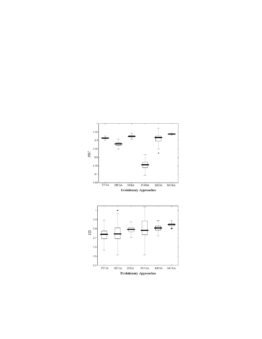
T
AN
,
K
HOR
,
L
EE
,
&
S
ATHIKANNAN
206
strong conclusion. However, as the average performance is concerned (see bold horizontal line in
the box plots), SPEA, MIGA and MOEA outperform others slightly and are more consistent in
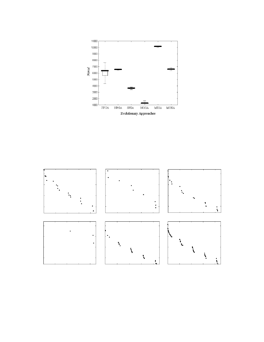
terms of the measure of UD. Figure 21 shows the distribution of Neval (number of function
evaluation) performed by each algorithm in a specified time. More function evaluations in a fixed
CPU time indirectly indicates that less CPU time is required by the algorithm. Intuitively, this
means less computational efforts are required by the algorithm to find the trade-offs. As shown in
Figure 21, MIGA requires the least algorithm effort while the performances of FFGA, NPGA and
MOEA are moderate in terms of Neval. It can also be observed that SPEA and NGGA are suitable
for problems with time-consuming function evaluations: the effects in algorithm effort become less
significant in these problems. In summary, the results show that MOEA requires moderate
computational effort and exhibits a relatively good performance in terms of SSC and UD on the test
problem, as compared to other MO evolutionary optimization methods in this study.
Figure 19: Box Plot of SSC
Figure 20: Box Plot of UD
A
N
E
VOLUTIONARY
A
LGORITHM FOR
M
ULTI
-
OBJECTIVE
O
PTIMIZATION
207
Figure 21: Box Plot of Neval
Figure 22 shows the distribution of non-dominated individuals in the objective domain, where
the range of each axis is identical to the range shown in Figure 18. For each algorithm, the
distribution is the best selected, among the 30 independent runs, with respect to the measure of SSC.
It can be seen from Figure 22 that MOEA benefits from evolving more non-dominated individuals
than the other methods. MOEA’s individuals are also better distributed within the trade-off region.
FFGA
NPGA
SPEA
NGGA
MIGA
MOEA
Figure 22: Best Selected Distribution of Non-dominated Individuals from Each Algorithm with
Respect to the Measure of SSC
T
AN
,
K
HOR
,
L
EE
,
&
S
ATHIKANNAN
208
5. Application to Practical Servo Control System Design
5.1 The Hard Disk Drive Servo System
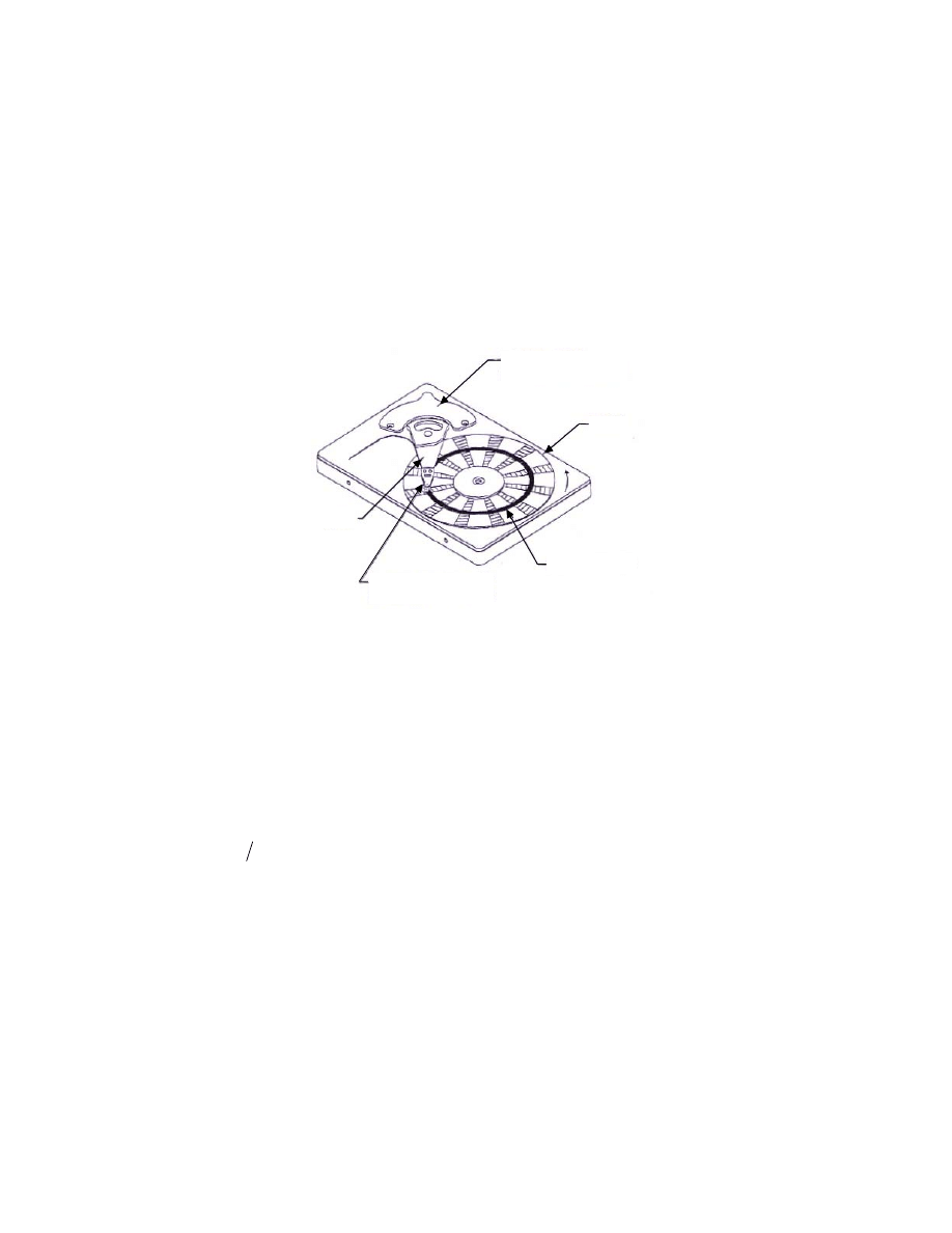
A typical plant model of hard disk drive (HDD) servo system includes a driver (power amplifier), a
VCM (Voice Coil Motor) and a rotary actuator that is driven by the VCM. Figure 23 (Goh et al.
2001) shows a basic schematic diagram of a head disk assembly (HDA), where several rotating
disks are stacked on the spindle motor shaft.
DATA TRACK
SUSPENSION AND
RECORDING HEAD
ARM
VOICE COIL MOTOR
ACTUATOR
DISK
Figure 23: A HDD with a Single VCM Actuator Servo System
The dynamics of an ideal VCM actuator is often formulated as a second-order state-space model
(Weerasooriya, 1996),
u
K
v
y
K
v
y
v
y
+
=
0
0
0
0
&
&
(15)
where u is the actuator input (in volts), y and v are the position (in tracks) and the velocity of the
R/W head, K
v
is the acceleration constant and K
y
the position measurement gain,
where
m
K
K
t
y
=
with K
t
being the current-force conversion coefficient and m being the mass of
the VCM actuator. The discrete-time HDD plant model used for the evolutionary servo controller
design in this study is given as (Tan et al. 2000),
u
k
x
k
x
+
=
+
664
.
1
384
.
1
)
(
1
0
664
.
1
1
)
1
(
(16)
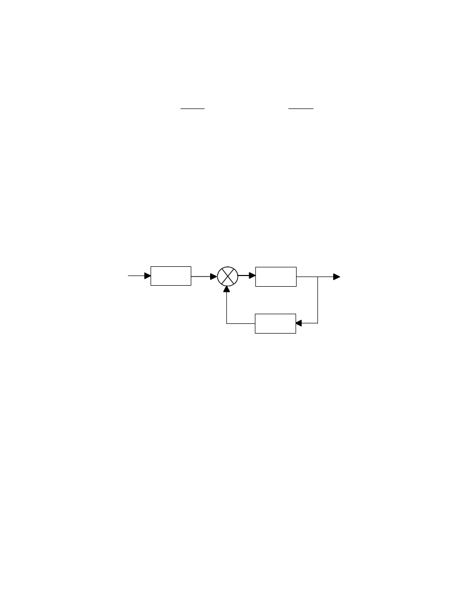
5.2 Evolutionary HDD Controller Design and Implementation
A two-degree-of-freedom (2DOF) control structure is adopted for the read/write head servo system
as shown in Figure 24. For simplicity and easy implementation, a simple first-order discrete-time
A
N
E
VOLUTIONARY
A
LGORITHM FOR
M
ULTI
-
OBJECTIVE
O
PTIMIZATION
209
controller with a sampling frequency of 4 kHz is used for the feedforward and feedback controllers,
which is in the form of
+
+
=
2
1
ff
z
ff
z
K
K
f
p
+
+
=
2
1
fb
z
fb
z
K
K
b
s
(17)
respectively. The control objective during the tracking in HDD is to follow the destination track
with a minimum tracking error. Note that only time domain performance specifications are
considered in this paper, and the design task is to search for a set of optimal controller parameters
{K
f
, K
b
, ff
1
, ff
2
, fb
1
, fb
2
} such that the HDD servo system meets all design requirements. These
requirements are that overshoots and undershoots of the step response should be kept less than 5%
since the head can only read or write within
±5% of the target; the 5% settling time in the step
response should be less than 2 milliseconds and settle to the steady-state as quickly as possible
(Goh et al. 2001). Besides these performance specifications, the system is also subject to the hard
constraint of actuator saturation, i.e., the control input should not exceed
±2 volts due to the
physical constraint on the VCM actuator.
Feedback controller
+
Feedforward
controller
y
u
r
Plant
VCM
K
s
K
p
-
Figure 24: The Two Degree-of-freedom Servo Control System
The multi-objective evolutionary algorithm (MOEA) proposed in this paper has been embedded
into a powerful GUI-based MOEA toolbox (Tan et al. 2001b) for ease-of-use and for
straightforward application to practical problems. The toolbox is developed under the Matlab (The
Math Works, 1998) programming environment, which allows users to make use of the versatile
Matlab functions and other useful toolboxes such as Simulink (The Math Works, 1999). It allows
any trade-off scenario for MO design optimization to be examined effectively, aiding
decision-making for a global solution that best meets all design specifications. In addition, the
toolbox is equipped with a powerful graphical user interface (GUI) and is ready for immediate use
without much knowledge of evolutionary computing or programming in Matlab. A file handling
capability for saving all simulation results and model files in a Mat-file format for Matlab or
text-file format for software packages like Microsoft Excel is also available in the toolbox. Through
the GUI window of MOEA toolbox, the time domain design specifications can be conveniently set
as depicted in Figure 25, where Tr, OS, Ts, SSE, u and ue represents the rise time, overshoot,
settling time, steady-state error, control input and change in control input, respectively.
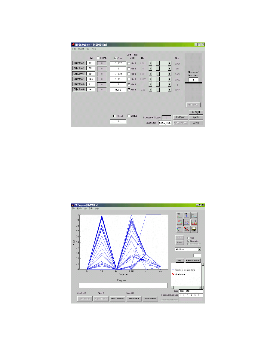
T
AN
,
K
HOR
,
L
EE
,
&
S
ATHIKANNAN
210
Figure 25: MOEA GUI Window for Settings of Design Specifications
The simulation adopts a generation and population size of 200, and all the design specifications
listed in Figure 25 have been successfully satisfied at the end of the evolution. The design trade-off
graph is shown in Figure 26, where each line representing a solution found. The x-axis shows the
design specifications and the y-axis shows the normalized cost for each objective. Clearly,
trade-offs between adjacent specifications result in the crossing of the lines between them (e.g.,
steady-state error (SSE) and control effort (u)), whereas concurrent lines that do not cross each
other indicating the specifications do not compete with one another (e.g., overshoots (OS) and
settling time (Ts)).
Figure 26: Trade-off Graph of the HDD Servo Control System Design
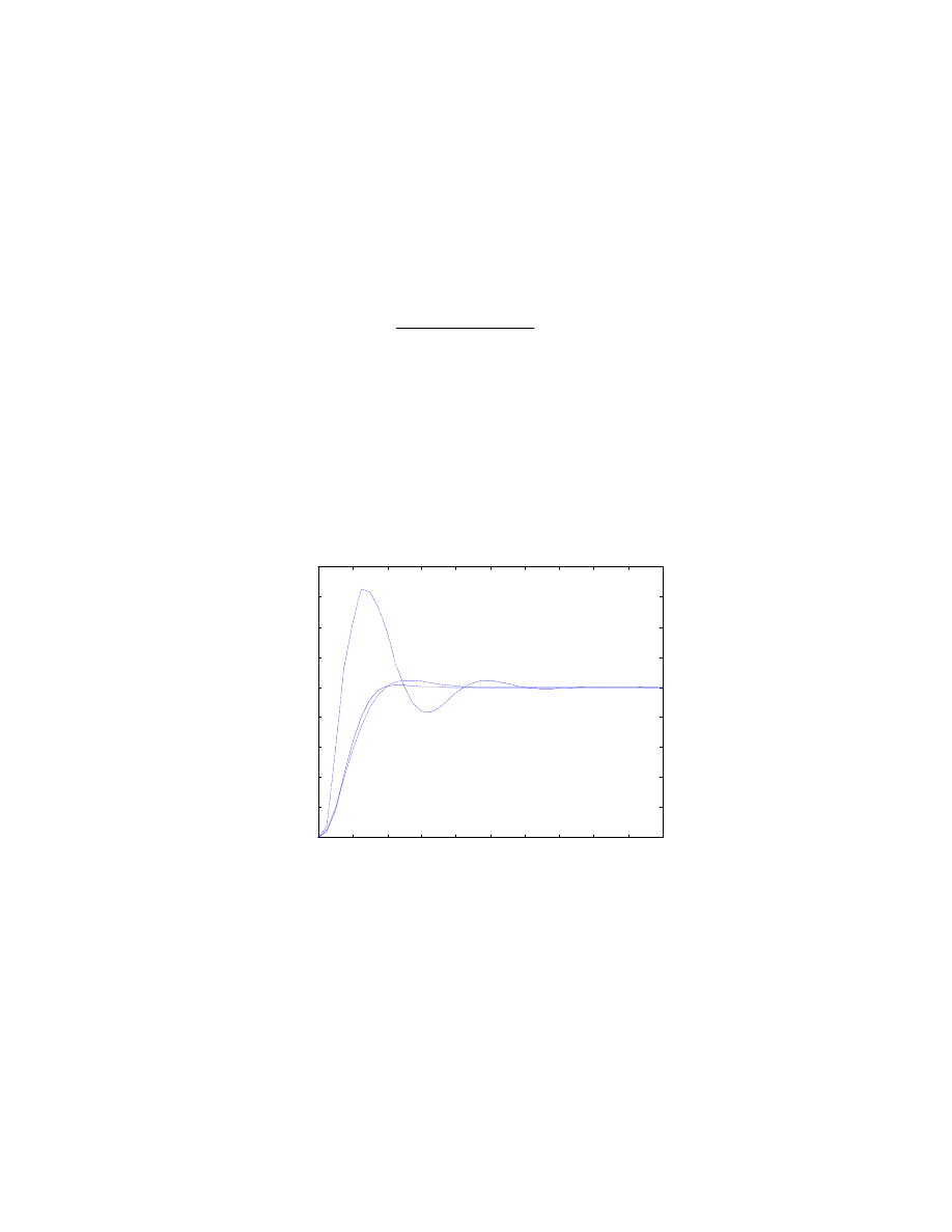
A
N
E
VOLUTIONARY
A
LGORITHM FOR
M
ULTI
-
OBJECTIVE
O
PTIMIZATION
211
The closed-loop step response of the overall system for an arbitrary selected set of MOEA
designed 2DOF controller parameters given as {K
f
, K
b
, ff
1
, ff
2
, fb
1
, fb
2
} = {0.029695, -0.58127,
0.90279, -0.3946, -0.70592, 0.83152} is shown in Figure 27. With a sampling frequency of 4 kHz,
the time domain closed-loop performance of the evolutionary designed controller has been
compared with the manually designed discrete-time PID controller as given in Eq. 18 (Goh et al.
2001) as well as the Robust and Perfect Tracking (RPT) controller (Goh et al. 2001) as given in Eq.
19,
)
(
25
.
0
25
.
1
1
.
0
23
.
0
13
.
0
2
2
y
r
z
z
z
z
u
−
+
−
+
−
=
(18)
)
(
18
.
0
)
(
04
.
0
)
(
10
43
.
3
)
(
)
(
453681
)
(
15179
)
(
04
.
0
)
1
(
7
k
y
k
r
k
x
k
u
k
y
k
r
k
x
k
x
−
+
×
−
=
−
+
−
=
+
−
(19)
It can be seen in Figure 27 that the evolutionary designed 2DOF controller has outperformed
both the PID and RPT controllers, with the fastest rise time, smallest overshoots and shortest
settling time in the closed-loop response. Its control performance is excellent and the destination
track crossover occurs at approximately 1.8 milliseconds.
0
0.001 0.002 0.003 0.004 0.005 0.006 0.007 0.008 0.009
0.01
0
0.2
0.4
0.6
0.8
1
1.2
1.4
1.6
1.8
: MOEA Based 2DOF Controller
: PID Controller
Time in Seconds
H
ead Po
si
tion
(Tra
cks)
: RPT Controller
1
2
3
1
3
2
Figure 27: Closed-loop Servo System Responses with Evolutionary 2DOF, RPT and PID
Controllers
The performance of the evolutionary 2DOF servo control system was further verified and tested
on the physical 3.5-inch HDD with a TMS320 digital signal processor (DSP) and a sampling rate of
4 kHz. The R/W head position was measured using a laser doppler vibrometer (LDV) and the
resolution used was 1
µm/volt. Real-time implementation result of the evolutionary HDD servo
control system is given in Figure 28, which is consistent with the simulated step response in Figure
27, and shows an excellent closed-loop performance.
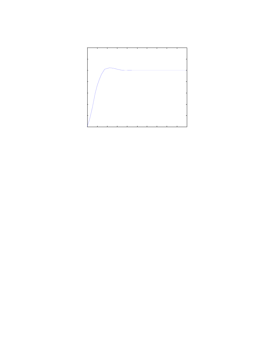
T
AN
,
K
HOR
,
L
EE
,
&
S
ATHIKANNAN
212
0
0.001 0.002 0.003 0.004 0.005 0.006 0.007 0.008 0.009
0.01
0
0.2
0.4
0.6
0.8
1
1.2
1.4
Time in Seconds
T
rack
s (
Ac
tu
a
to
r O
u
tput
)
Output Response
Figure 28: Real-time Implementation Response of the Evolutionary 2DOF Servo System
6. Conclusions
This paper has presented a multi-objective evolutionary algorithm (MOEA) with a new
goal-sequence domination scheme to allow advanced specifications such as hard/soft priorities and
constraints to be incorporated for better decision support in multi-objective optimization. In
addition, a dynamic fitness sharing scheme that is simple in computation and adaptively based upon
the on-line population distribution at each generation has been proposed. Such a dynamic sharing
approach avoids the need for a priori parameter settings or user knowledge of the usually unknown
trade-off surface often required in existing methods. The effectiveness of the proposed features in
MOEA has been demonstrated by showing that each of the features contains its specific merits and
usage that benefit the performance of MOEA. In comparison with other existing evolutionary
approaches, simulation results show that MOEA has performed well in the diversity of
evolutionary search and uniform distribution of non-dominated individuals along the final
trade-offs, without significant computational effort. The MOEA has been applied to the practical
engineering design problem of a HDD servo control system. Simulation and real-time
implementation results show that the evolutionary designed servo system provides excellent
closed-loop transient and tracking performance.
Acknowledgements
The authors wish to thank Andrew Moore and the anonymous reviewers for their valuable
comments and helpful suggestions which greatly improved the paper quality.

A
N
E
VOLUTIONARY
A
LGORITHM FOR
M
ULTI
-
OBJECTIVE
O
PTIMIZATION
213
References
Borges, C. C. H., & Barbosa, H. J.C. (2000). A non-generational genetic algorithm for
multiobjective optimization. IEEE Congress on Evolutionary Computation, 1, 172-179.
Chambers, J. M., Cleveland, W. S., Kleiner, B., & Turkey, P. A. (1983). Graphical Methods for
Data Analysis, Wadsworth & Brooks/Cole, Pacific CA.
Coello Coello, C. A. (1996). An Empirical Study of Evolutionary Techniques for Multiobjective
Optimization in Engineering Design, Ph.D. Thesis, Dept. of Computer Science, Tulane University,
New Orleans, LA.
Coello Coello, C. A. (1999). A Comprehensive Survey of Evolutionary-Based Multiobjective
Optimization Techniques. Knowledge and Information Systems, 1(3), 269-308.
Deb, K. (1999). Evolutionary algorithms for multi-criterion optimization in engineering design. In
Miettinen. Evolutionary Algorithms in Engineering and Computer science: Recent Advances in
Genetic Algorithms, Evolution Strategies, Evolutionary Programming, Genetic Programming, and
Industrial Applications, Wiley, New York, 135-161.
Deb, K. (2001). Multi-objective Optimization using Evolutionary Algorithms. John Wiley & Sons,
London.
Fonseca, C. M. (1995). Multiobjective Genetic Algorithms with Application to Control Engineering
Problems. Ph.D. Thesis, Dept. of Automatic Control and Systems Engineering, University of
Sheffield, UK.
Fonseca, C. M., & Fleming, P. J. (1993). Genetic algorithm for multiobjective optimization,
formulation, discussion and generalization. In (Forrest, 1993), 416-423.
Fonseca, C. M. & Fleming, P. J., (1998). Multiobjective optimization and multiple constraint
handling with evolutionary algorithms – Part I: A unified formulation. IEEE Trans. on System, Man,
and Cybernetics-Part A: System and Humans, 28(1), 26-37.
Goh, T. B., Li, Z. M., Chen, B. M., Lee, T. H., & Huang, T., (2001). Design and implementation of
a hard disk drive servo system using robust and perfect tracking approach. IEEE Trans. on Control
Systems Technology, 9(2), 221-233.
Goldberg, D. E., & Richardson, J. (1987). Genetic algorithms with sharing for multimodal function
optimization. Proc. 2
nd
Int. Conf. on Genetic Algorithms, 41-49.
Goldberg, D. E. (1989). Genetic Algorithms in Search, Optimization and Machine Learning.
Addison-Wesley, Reading, Massachusetts.
Grace, A. (1992). Optimisation Toolbox User’s Guide, The MathWorks, Inc.
Holland, J. H. (1975). Adaptation in Natural and Artificial Systems. University of Michigan, Ann
Harbor.

T
AN
,
K
HOR
,
L
EE
,
&
S
ATHIKANNAN
214
Horn, J., & Nafpliotis, N. (1993). Multiobjective Optimization Using the Niche Pareto Genetic
Algorithm. IlliGAL Report 93005, University of Illinois, Urbana, Illinois, USA.
Luus, R., Hartig, F. & Keil, F. J., (1995). Optimal drug scheduling of cancer chemotherapy by
direct search optimization. Hungarian Journal of Industrial Chemistry, 23, 55-58.
Marcu, T. (1997). A Multiobjective evolutionary approach to pattern recognition for robust
diagnosis of process faults. Proc. of IFAC Fault Detection, Supervision and Safety for Technical
Process, UK, 1183-1188.
Michalewicz, Z., & Schoenauer, M., (1996). Evolutionary algorithms for constrained parameter
optimization problems. Evolutionary Computation, 4(1), 1-32.
Miller, B. L., & Shaw, M. J. (1996). Genetic algorithms with dynamic niche sharing for multimodal
function optimization. IEEE Conf. on Evolutionary Computation, Japan, 786-791.
Murata, T., & Ishibuchi, H., (1996). Multi-objective genetic algorithm and its applications to
flowshop scheduling. Int. Journal of Computers and Engineering, 957-968.
Osyczka, A. (1984). Multicriterion Optimisation in Engineering. Ellis Horwood, Chichester.
Schaffer, J. D. (1985). Multiple-objective optimization using genetic algorithm. Proc. of first Int.
Conf. on Genetic Algorithms, 93-100.
Tan, K. C., Lee, T. H., & Khor, E. F. (1999). Evolutionary algorithms with goal and priority
information for multi-objective optimization. IEEE Congress on Evolutionary Computation, 1,
106-113.
Tan, K. C., Sathikannan, R., Tan, W. W., Loh, A. P., Lee, T. H., & Mamun, A. Al. (2000)
Evolutionary Design and Real-Time Implementation of a Hard Disk Drive Servo Control System.
Int. Conf. on Control 2000, University of Cambridge, UK, Section 6C.
Tan, K. C., Lee, T. H., & Khor, E. F., (2001a). Evolutionary algorithms for multi-objective
optimization: Performance assessments and comparisons. IEEE Congress on Evolutionary
Computation, 2, 979-986.
Tan, K. C., Lee, T. H., Khoo, D., & Khor, E. F., (2001b). A multi-objective evolutionary algorithm
toolbox for computer-aided multi-objective optimization. IEEE Trans. on Systems, Man and
Cybernetics - Part B: Cybernetics, 31(4), 537-556.
The Math Works, Inc. (1998). Using MATLAB, Version 5.
The Math Works, Inc. (1999). Simulink: User's Guild, Version 3.
Van Veldhuizen, D. A., & Lamont, G. B. (1998). Multiobjective evolutionary algorithm research:
A history and analysis. Technical Report TR-98-03, Dept. of Electrical and Computer Eng.,
Graduate School of Eng., Air Force Institute of Technology, Wright-Patterson AFB, Ohio.

A
N
E
VOLUTIONARY
A
LGORITHM FOR
M
ULTI
-
OBJECTIVE
O
PTIMIZATION
215
Weerasooriya, S. (1996). The Basic Servo Problem: Technical Report. Data Storage Institute,
National University of Singapore, Singapore.
Zitzler, E., & Thiele, L., (1999). Multiobjective evolutionary algorithms: A comparative case
study and the strength Pareto approach. IEEE Trans. on Evolutionary Computation, 3(4), 257-271.
Wyszukiwarka
Podobne podstrony:
więcej podobnych podstron