Monitoring the Risk of High Frequency Returns on Foreign Exchange

Real-Time Multivariate Density Forecast Evaluation and Calibration:

Monitoring the Risk of High-Frequency Returns on Foreign Exchange

Francis X. Diebold

Jinyong Hahn

Anthony S. Tay

University of Pennsylvania University of Pennsylvania National University

Stern School, NYU

and M.I.T.

of Singapore

and NBER

This Draft/Print: August 26, 1998

Wide Web at http://www.ssc.upenn.edu/~diebold/ and may be freely reproduced for

educational and research purposes, so long as it is not altered, this copyright notice is

reproduced with it, and it is not sold for profit.

Abstract: We provide a framework for evaluating and improving multivariate density

forecasts. Among other things, the multivariate framework lets us evaluate the adequacy of

density forecasts involving cross-variable interactions, such as time-varying conditional

correlations. We also provide conditions under which a technique of density forecast

“calibration” can be used to improve deficient density forecasts. Finally, motivated by recent

advances in financial risk management, we provide a detailed application to multivariate high-

frequency exchange rate density forecasts.

Acknowledgments: Helpful comments were provided by Jose Campa, Neil Shephard, Charlie

Thomas, and Mike West, as well as seminar and conference participants at Stern, Wharton,

and Olsen & Associates. All remaining inadequacies are ours alone. For support we thank

the National Science Foundation, the Sloan Foundation, the University of Pennsylvania

Research Foundation, and the National University of Singapore.

Diebold, F.X., Hahn, J. and Tay, A. (1999),

"Multivariate Density Forecast Evaluation and Calibration in Financial Risk Management: High-Frequency Returns on Foreign Exchange,"

Review of Economics and Statistics, 81, 661-673.

1. Introduction

The forecasting literature has traditionally focused primarily on point forecasts.

Recently, however, attention has been given to interval forecasts (Chatfield, 1993) and

density forecasts (Diebold, Gunther and Tay, 1998). The reasons for the recent interest in

interval and density forecasts are both methodological and substantive. On the

methodological side, recent years have seen the development of powerful models of time-

varying conditional variances and densities (Bollerslev, Engle and Nelson, 1994; Ghysels,

Harvey and Renault, 1996; Hansen, 1994; Morvai, Yakowitz and Algoet, 1997). On the

substantive side, density forecasts and summary statistics derived from density forecasts have

emerged as a key part of the explosively-growing field of financial risk management (Duffie

and Pan, 1997; Jorion, 1997), as well in as more traditional areas such as macroeconomic

inflation forecasting (Wallis, 1998). Moreover, explicit use of predictive densities has long

been a prominent feature of the Bayesian forecasting literature (Harrison and Stevens, 1976;

West and Harrison, 1997), and recent advances in Markov Chain Monte Carlo (Gelman,

Carlin, Stern and Rubin, 1995) have increased the pace of progress. The closely related

“prequential” Bayesian literature (Dawid, 1984) also features density forecasts prominently.

Interest in forecasts of various sorts creates a derived demand for methods of

evaluating

forecasts. In parallel with the historical emphasis on point forecasts, most

literature has focused on the evaluation of point forecasts (Diebold and Lopez, 1996), but

recent interest in interval and density forecasts has spurred development of methods for their

evaluation (Christoffersen, 1998; Diebold, Gunther and Tay, 1998). Diebold, Gunther and

Tay, in particular, motivate and approach the problem of density forecast evaluation from a

Some progress, however, is also being made at evaluating density forecasts produced

from estimated models; see Bai (1997) and Inoue (1997).

risk management perspective, drawing upon an integral transform dating at least to Rosenblatt

(1952), extended by Seillier-Moiseiwitsch (1993) and used creatively by Shephard (1994).

Here we extend the density forecast evaluation literature in three ways. First, we treat

the multivariate case, which lets us evaluate the adequacy of density forecasts involving

cross-variable interactions, such as time-varying conditional correlations, which are crucial in

financial settings. Second, we provide conditions under which a technique of density forecast

“calibration” can be used to improve deficient density forecasts. Finally, we provide a

detailed application to the evaluation of density forecasts of multivariate high-frequency

exchange rates, which is of direct substantive interest in addition to illustrating the ease with

which the methods can be implemented.

2. Density Forecast Evaluation and Calibration

We begin with a brief summary of certain key univariate evaluation results from

Diebold, Gunther and Tay (1998), in order to establish ideas and fix notation. We then

describe our methods of univariate calibration, after which we extend both the evaluation and

calibration methods to the multivariate case. Throughout, we intentionally ignore parameter

estimation uncertainty. We take density forecasts as primitives, and in particular, we do not

require that they be based on an estimated model. We take this approach because many

density forecasts of interest do not come from models with estimated parameters, as for

example when density forecasts are extracted from surveys (Diebold, Tay and Wallis, 1997)

or from prices of options written at different strike prices (Aït-Sahalia and Lo, 1998;

t 1

(u)du

t 1

) =

t 1

)

f(P

t 1

)

t 1

) =

f(P

t 1

)

t 1

)

t 1

))

)

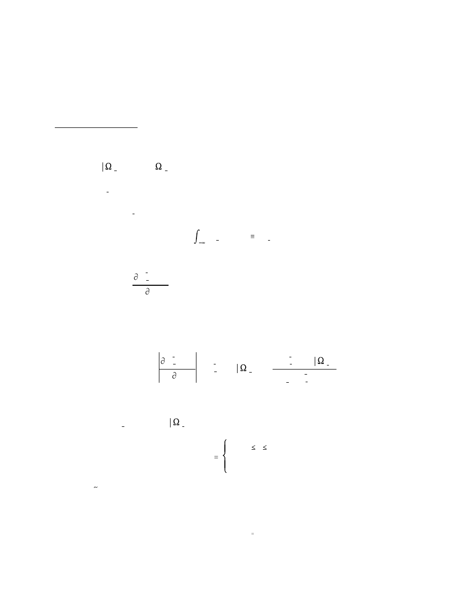
1 if 0 z

0 otherwise,

f(y

t 1

)

t 1

)

t 1

)

t 1

)

t 1

) = f(y

t 1

)

U(0,1)

}

t 1

Soderlind and Svensson, 1997; Campa, Chang and Reider, 1998). This is the case for some

of the exchange rate density forecasts that we evaluate in section 4.

Univariate Evaluation

Consider one arbitrary period, t, and let be the variable of interest with conditional

density

, where

represents the collection of past information available at time

t-1, and let

be a density forecast of . Let be the probability integral transform of

with respect to

; that is,

Then assuming that

is continuous and non-zero over the support of , has

support on the unit interval with density function

In particular, if

, then

so that

Now consider a series of m density forecasts and realizations, rather than just one.

Diebold, Gunther and Tay (1998) show that if

is a series of realizations generated

f(y

m 1

) = p

m 1

) q

m 1

f(y

m 1

) = p

m 1

) q(z

m 1

{f(y

t 1

)}

t 1

)}

t 1

{f(y

t 1

)}

t 1

}

t 1

)}

t 1

}

t 1

iid

U(0,1).

ˆy

m 1

We thank Charlie Thomas for pointing out that the basic idea of univariate density

forecast calibration traces at least to Fackler and King (1990). Shortly, however, we will

extend the calibration idea to the multivariate case. Moreover, we will emphasize that density

forecast calibration is not universally applicable and develop a sufficient condition for its

application in both the univariate and multivariate cases.

from the series of conditional densities

, and if a series of 1-step-ahead density

forecasts

coincides with

, then assuming a non-zero Jacobian

with continuous partial derivatives, the series of probability integral transforms of

with respect to

is iid U(0,1). That is,

Thus, to assess

whether a series of density forecasts coincides with the corresponding series of true

conditional densities, we need only assess whether an observed series is iid U(0,1).

Univariate Calibration

An important practical question is how to improve suboptimal forecasts. In the point

forecast case, for example, we can regress the y's on the 's (the predicted values) and

potentially use the estimated relationship to construct an improved point forecast. Such a

regression is sometimes called a Mincer-Zarnowitz regression, after Mincer and Zarnowitz

(1969). In this paper we will use an analogous procedure, which we call density forecast

“calibration,” for improving density forecasts that produce an iid but non-uniform z series.

Suppose that we are in period m and possess a density forecast of

. From our

earlier discussion,

But if z is iid, then we can drop the subscript on q and write

t 1

, y

, ..., y

) = p

t 1

| y

N 1,t

, ..., y

)

t 1

| y

) p

t 1

q(z

m 1

)

f(y

m 1

)

q(z

m 1

)

ˆq(z

m 1

)

}

t 1

ˆf(y

m 1

)

( y

, y

,..., y

)

Note that z is uniquely determined by y, so that for any given value of y, we can

always compute f(y) as p(y)q(z).

Thus if we knew

, we would know the actual conditional distribution

Because

is unknown, we use an estimate

formed using

to construct

an estimate

. In finite samples, of course, there is no guarantee that the

“improved” forecast will actually be superior to the original, because it is based on an

estimate of q rather than the true q, and the estimate could be very poor. The practical

efficacy of our improvement methods is an empirical matter, which will be assessed shortly,

but with the large sample sizes typically available in financial applications we expect that

precise estimation of q will often be straightforward.

Multivariate Evaluation

The principles that govern the univariate techniques discussed thus far extend readily

to the multivariate case. Suppose that y is now an Nx1 vector, and that we have a series of m

multivariate forecasts and their corresponding multivariate realizations. Further suppose that

we are able to factor each period’s joint forecast into the product of the conditionals,

Then for each period we can transform each element of the multivariate observation

by its corresponding conditional distribution. This procedure produces a set

of N z series that will be iid U(0,1) individually, and also when taken as a whole, if the

multivariate density forecasts are correct. The proof of this assertion is obtained by simply

arranging the multivariate series as a series of univariate observations comprising

{... , y

, y

,..., y

, ...}

t 1

, y

)

t 1

) p

t 1

| y

)

t 1

, y

)

t 1

) p

t 1

| y

, z

2|1

, z

and z

1|2

t 1

)

i| j

t 1

| y

)

, z

2|1

, z

and z

1|2

{..., z

1, t

, z

2|1, t

, ...}

{..., z

2, t

, z

1|2, t

, ...}

That is, we begin with had m observations on an N-variate variable, and we convert

them to a univariate series with Nm observations.

. The result for the univariate case can then be applied to show that

the resulting Nm vector z is iid U(0,1), and hence the z series corresponding to any particular

series of conditional forecasts is also iid U(0,1).

Note that N! z series can be produced, depending on how the joint density forecasts

are factored, giving us a wealth of information with which to evaluate the forecasts. To take

the bivariate case as an example, we can decompose the forecasts in two ways:

(i)

and

(ii)

t = 1, ..., m, and label the respective z series

, where we obtain by

taking the probability integral transform of with respect to

, and we obtain

transforming with respect to

. Good multivariate forecasts will produce

that are each iid U(0, 1), as well as combined series

and

that are also iid U(0,1).

In many cases of economic and financial interest, such as the application to density

forecasting of DM/$ and Yen/$ returns in section 4 of this paper, the dimension N of the set

of variables being forecast is low. A classic example is density forecasting of returns across

different aggregate asset classes, such as equity, foreign exchange and fixed income. In such

cases, it is straightforward to examine and learn from each of the N! sets of z series.

Sometimes, however, N may be large, as for example when a density forecast is generated for

each of the stocks in a broad-based market index, such as the S&P 500, in which case

f(y

1,m 1

, y

2,m 1

,..., y

N,m 1

)

1,m 1

, y

2,m 1

,..., y

N,m 1

) q(z

1,m 1

, z

2,m 1

,..., z

N,m 1

f(y

1,m 1

, y

2,m 1

,..., y

N,m 1

)

i 1

i,m 1

| y

i 1,m 1

,..., y

1,m 1

) q(z

i,m 1

| z

i 1,m 1

,..., z

1,m 1

) .

ˆf(y

1,m 1

, y

2,m 1

,..., y

N,m 1

)

1,m 1

, y

2,m 1

,..., y

N,m 1

) ˆq(z

1,m 1

, z

2,m 1

,..., z

N,m 1

ˆf(y

1,m 1

, y

2,m 1

,..., y

N,m 1

)

i 1

i,m 1

| y

i 1,m 1

,..., y

1,m 1

) ˆq(z

i,m 1

| z

i 1,m 1

,..., z

1,m 1

) .

methods such as those of Clements and Smith (1998) may be used to aggregate the

information in the individual z series.

Multivariate Calibration

In parallel with the key formula underlying our discussion of univariate calibration, in

the multivariate case we have that

Moreover, factoring both of the right-hand-side densities, we can write the formula in a way

that precisely parallels our multivariate evaluation framework,

As before, an estimate of q may be used to implement the calibration empirically, yielding

Note that the multivariate calibrating density is the same (in population), regardless of which

of the possible N! factorizations is used.

3. More on Density Forecast Calibration

Here we elaborate on various aspects of density forecast calibration. First we give a

sufficient condition for an iid integral transform series, which is required for application of the

calibration method. Next we discuss subtleties associated with estimation of the density of an

integral transform, which by construction has compact support on the unit interval. Finally,

f(y

t 1

)

(

t 1

)

µ(

t 1

)

(

t 1

)

f(y

t 1

)

t 1

)

f(y

t 1

)

µ(

t 1

)

(

t 1

)

t 1

)

µ(

t 1

)

(

t 1

)

we show how the calibration method can be used to generate good density forecasts even

when the conditional density is unknown. In this section we use the generic notation “z” to

denote an integral transform; it is a scalar integral transform in the univariate case and a

vector of integral transforms in the multivariate case.

Conditions Producing an iid z Series

In empirical work, the legitimacy of the assumption that z is iid can be assessed in a

number of ways, ranging from examination of correlograms of various powers of z to formal

tests such as those discussed in Brock, Hsieh and LeBaron (1991). It is nevertheless desirable

to characterize theoretically the conditions under which z will be iid, in order to deepen our

understanding of whether and when we can reasonably hope for an iid z series. Here we

establish a sufficient condition: if the 1-step-ahead density

belongs to a location-

scale family, and if the forecast

adequately captures dynamics (in a sense to be made

precise shortly) but is mistakenly assumed to be in another location-scale family, then z will

be iid.

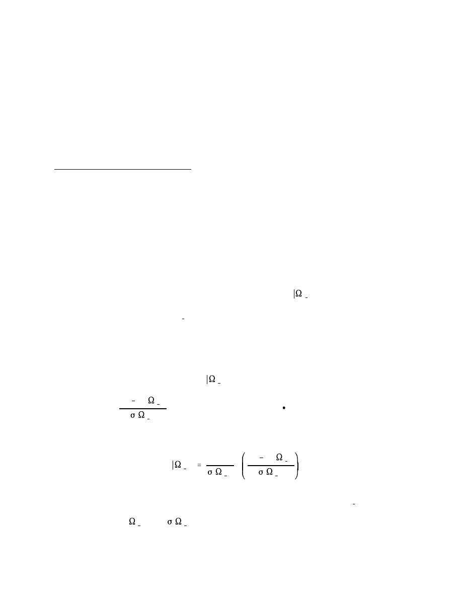
More precisely, suppose that

belongs to a location-scale family; that is, the

random variable

is iid with unknown density f( ). It then follows that

Now suppose that we misspecify the model by another location-scale family,

, in

which we specify

and

correctly, in spite of the fact that we use an incorrect

t 1

)

(

t 1

)

µ(

t 1

)

(

t 1

)

t 1

)dy

(

t 1

)

µ(

t 1

)

(

t 1

)

µ(

t 1

)

(

t 1

)

(

t 1

)

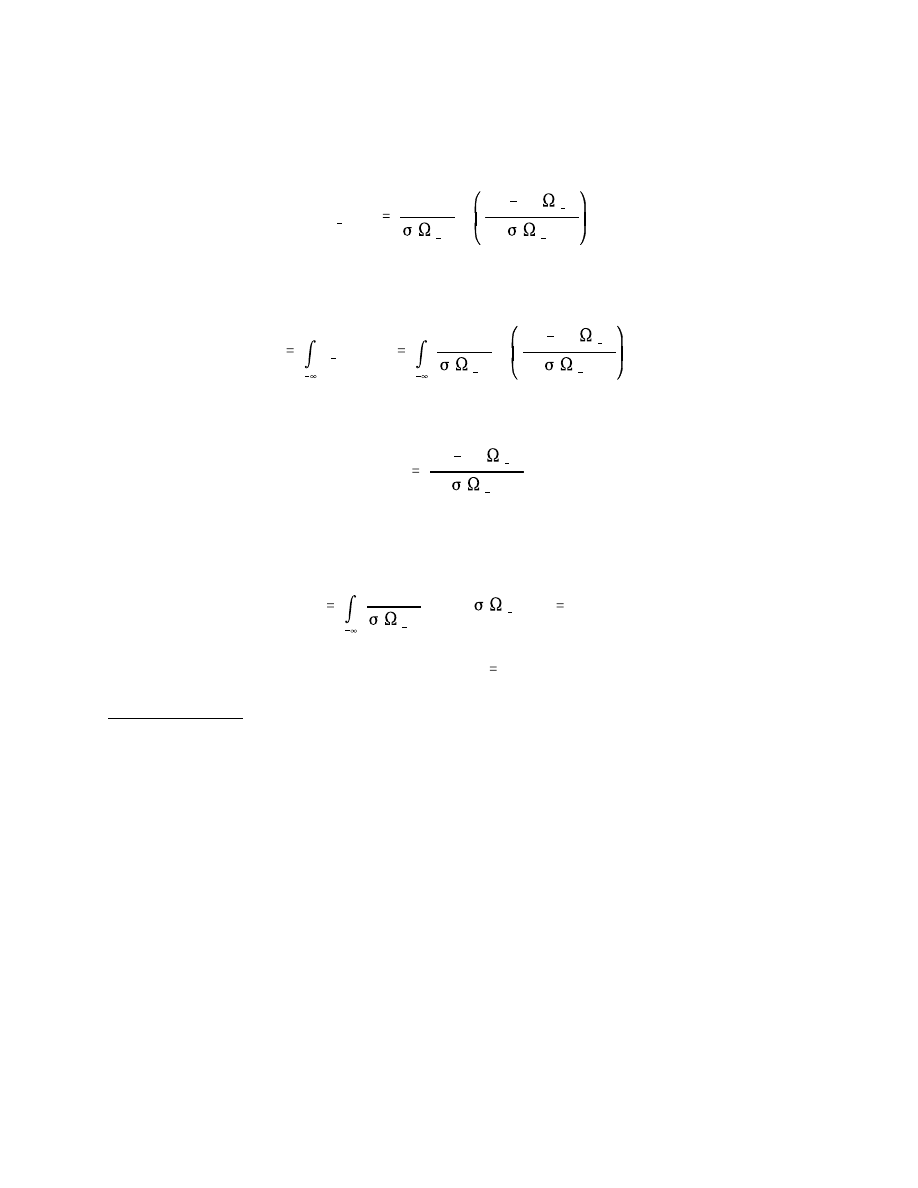
p(u

) (

t 1

)du

P(u

)

conditional density. Thus we issue the density forecast

The probability integral transform of the realization with respect to the forecast is therefore

Now make the change of variable

which yields

But this means that z is iid, as claimed, because

and is iid.

Estimation of q(z)

Estimation of q(z) requires care, because z has support only on the unit interval. One

could use a global smoother on the unit interval, such as a simple two-parameter beta

distribution, but the great workhorse beta family is unfortunately not flexible enough to

accommodate the multimodal shapes of q(z) that arise routinely, as documented in Diebold,

Gunther and Tay (1998). One could perhaps stay in the global smoothing framework by

using some richer parametric family or a series estimator, as discussed for example by Härdle

(1991).

In keeping with much of the recent literature, however, we prefer to take a local

ˆq(z)

t 1

z z

E[ˆq(z)]

1
b

K u z

q(u) du

q(z)

1 z

z
b

K(v)dv bq (z)

1 z

z
b

K(v)vdv 1

q (z)

1 z

z
b

K(v)v

o(b

, ..., z

q(z)

ˆq(z)

q(z)

K( )

b>0

smoothing approach, as for example with a kernel density estimator. But it has long been

recognized that standard kernel estimation of densities with bounded support suffers from a

“boundary problem” in that the density estimates at the boundaries are biased. One cause of

this problem is that near the boundary approximately half of the kernel mass falls outside the

range of the data (assuming a symmetric kernel). Therefore, kernel density estimates near

boundaries have expectations approximately equal to half the true underlying density.

Let us elaborate. For i.i.d. data

with sufficiently smooth density

on [0,

1], the kernel estimator

where

is a symmetric and sufficiently smooth kernel of choice and

is bandwidth.

Begin by noting that

1 x

x
b

K(v) f(x bv) dv

E[ˆq(z)]

q(z) O(b

E[ˆq(0)]

q(0)

O(b)

E[ˆq(1)]

q(1)

O(b).

b 0

T .

See Härdle (1990, 130-131), for example, for related discussion in the context of

kernel regression, as opposed to density estimation.

Now suppose as usual that the bandwidth is chosen such that

and

For z

well in the interior of [0,1], we then have

On the other hand, the kernel density estimates have expectations approximately equal to only

half of the true underlying density at boundaries:

It can be shown that similar bias occurs at points near the boundaries.

There are a number of ways to address the boundary problem. One is to use a

modified kernel density estimator such as the one suggested by Müller (1993), which is

designed to have less bias near boundaries. Another local smoothing approach is to estimate

q(z) with a simple histogram. A histogram is a special type of kernel density estimator where

the kernel never exceeds the boundaries of the distribution. Therefore we expect that it would

not suffer from the problem associated with kernels that exceed the boundaries, and

F(y

1,m 1

,...,y

N,m 1

)

Q(P

1,m 1

,...,y

N,m 1

)),

ˆF(y

1,m 1

,...,y

N,m 1

)

ˆQ(P

1,m 1

,...,y

N,m 1

)).

experimentation revealed it to be superior in the present context; we make extensive use of

histograms as visual estimates of q(z) in the empirical application in section 5. Finally, we

can bypass the density estimation problem altogether by casting our evaluation and calibration

methods in terms of c.d.f.’s rather than densities, and using empirical c.d.f.’s instead of

estimated densities.

Alternatively, we may write the calibration formula in terms of joint c.d.f.’s rather than

joint densities, as

which we make operational by replacing population c.d.f.’s with estimated (empirical)

c.d.f.’s,

Although empirical c.d.f.’s are not as visually digestible as estimated densities, they have a

number of attractive features: they are guaranteed to be 0 for z=0 and 1 for z=1, and there is

no need for bandwidth selection bandwidth selection in the estimation of Q. We make

extensive use of empirical c.d.f.’s for doing the calibration transformations in the empirical

application in section 5.

Generating Density Forecasts When the Conditional Density is Unknown

It is interesting to note that our calibration methods can be used to generate density

forecasts even when the conditional density is unknown. Consider, for example, the problem

of 1-step-ahead density forecasting in models with unknown 1-step-ahead conditional density

and time-varying volatility. The problem is of intrinsic interest, and moreover, it is quite

general. In particular, it also covers h-step-ahead density forecasting, which in financial

See, for example, Duan (1995) and Duan, Gauthier and Simonato (1997).

contexts is equivalent to 1-step-ahead forecasting of h-period returns.

As is well known, even under heroic assumptions such as conditionally Gaussian 1-

step-ahead returns, the h-step-ahead conditional density, or equivalently the h-period return,

will not be Gaussian and has no known closed form. Several earlier papers bear on the

problem, but all are lacking in certain respects. Baillie and Bollerslev (1992), for example,

study h-step-ahead prediction but must assume a Gaussian 1-step-ahead conditional density

and even in that case provide only Cornish-Fisher approximations to the multi-step densities.

Engle and González-Rivera (1991) use a different but closely related strategy; let us

contrast the two. Engle and González-Rivera exploit the Bollerslev-Wooldridge (1992) result

that GARCH volatility parameters are consistently estimated by maximum likelihood even

when the conditional density is misspecified. Hence (assuming for convenience a zero

conditional mean) one can assume a Gaussian conditional distribution (incorrectly, in

general), maximize the Gaussian likelihood, and standardize the data by the estimated series

of conditional standard deviations. In large samples the resulting series will be iid but not, in

general, Gaussian; but its density can be estimated using nonparametric techniques.

In tackling this problem, our calibration procedure also exploits the Bollerslev-

Wooldridge (1992) quasi-MLE result. We proceed by maximizing the likelihood, which we

assume to be Gaussian (incorrectly, in general). We then take the estimated volatility

parameters and use them to make conditionally Gaussian density forecasts (again incorrectly),

and we compute the probability integral transforms of the realizations with respect to those

forecasts. In large samples, under the conditions given earlier, the series of integral

See, for example, Silverman (1986).

transforms will be iid but not U(0,1); we therefore calibrate the forecasts using either a

histogram or a c.d.f. fit to the series of integral transforms.

The key difference between the Engle-González-Rivera approach and our calibration

approach is that the first involves nonparametric estimation of a density with infinite support,

whereas the second maps the problem into one of nonparametric estimation of a density with

bounded support. Given that in risk management contexts our interest centers on tail events,

the Engle and González-Rivera approach may be problematic, due to the well-known

“bumpy-tail” problem. The bumpy-tail problem may be overcome by applying larger

bandwidths at the tails, but instead of applying some ad hoc method of choosing variable

bandwidth, the integral transformation implicitly provides an empirically reasonable variable

bandwidth, so long as the density forecasts are close to the true density. In addition, we note

that our procedure is not limited to the GARCH paradigm, and is applicable to any situation

where the forecasts generate z series that are iid. As discussed previously, extensions to

multivariate density forecasting contexts are also straightforward.

The empirical application to which we now turn illustrates all of the ideas developed

thus far: we begin by evaluating a series of multivariate density forecasts that are revealed to

be poor by virtue of associated iid but non-uniform integral transform series, we estimate the

appropriate calibrating density, and we use it to transform the poor density forecasts into good

ones.

4. Evaluating and Calibrating Multivariate Density Forecasts of High-Frequency

Returns on Foreign Exchange

See, for example, Anderson and Bollerslev (1997).

Here we present a detailed application of our methods of multivariate density forecast

evaluation and calibration to a bivariate system of asset returns. In particular, we study high-

frequency DM/$ and YEN/$ exchange rate returns, and we generate density forecasts from a

forecasting model in the tradition of JP Morgan’s RiskMetrics (JP Morgan, 1996), which is a

popular benchmark in the risk management industry.

We use our multivariate density forecast evaluation tools to assess the adequacy of the

RiskMetrics approximation the dynamics in high frequency exchange rate returns, as well as

the adequacy of the conditional normality assumption, after which we attempt to improve the

forecasts using calibration methods. We begin with a description of the data and a discussion

of the statistical properties of the returns series. We then describe the forecasting model, after

which we evaluate and calibrate the density forecasts that it produces.

Data

The data, kindly provided by Olsen and Associates, are indicative bid and ask quotes

posted by banks, spanning the period from January 1, 1996, to December 31, 1996. The data

are organized around a grid of half-hour intervals; Olsen provides the quotes nearest the half-

hour time stamps. Foreign exchange trading occurs around the clock during weekdays, but

trading is very thin during weekends, so we remove them, as is customary. We consider the

weekend to be the period from Friday 21:30 GMT to Sunday 21:00 GMT, as this period

appears to correspond most closely to the weekly blocks of zero returns. Thus a trading week

spans Sunday 21:30 GMT to Friday 21:00 GMT, and each of the five trading days therein

spans 21:30 GMT on one day to 21:00 GMT the next day. We label the days “Monday”

1
2

( x

t, ask

t, bid

)

t, ask/bid

ln x

t, ask/bid, previous

time

t, previous

time

t, previous

time

t, next

(ln x

t, ask/bid, next

ln x

t, ask/bid, previous

) .

t, ask/bid

t, ask/bid, previous/next

time

t, previous/next

t 1

through “Friday.” This layout implies that we have one partial week of data, followed by 51

full weeks, followed by another partial week of data. Each full week of data has 5x48=240

data points. The first partial week has 233 observations (just less than five days of data), and

the sample ends with a partial week of 102 observations (about 2 days), for a total of 12,575

observations.

Computing Returns

We compute returns by computing bid and ask rates at each grid point as the linear

interpolation of the nearest previous and subsequent quotes, as in Andersen and Bollerslev

(1997). The rate of return on the exchange rate is then the difference between the mid-point

of the log bid and ask rate at consecutive grid points. That is, letting

denote the log

ask / bid quote at the grid point t,

represent the nearest previous/next-

occurring bid or ask quote at time t, and

be the time between the grid point

and the previous/next quote, we obtain the exchange rate at time t, , as

where

The exchange rate return at time t, , is then

. It will sometimes be necessary

to refer to the return at a particular time of a particular day. In such cases, we will use

represent the return at time of day i.

The returns exhibit the MA(1) conditional mean dynamics commonly found in asset

returns. Because our focus in this paper is on volatility dynamics and their relation to density

, r

and |r

, i

2log|r

2logs

2logZ

forecasting, we follow standard practice and remove the MA(1) dynamics from each return.

We do so by fitting MA(1) models and treating the residuals as our returns series. Hereafter,

will refer to returns series with the MA(1) component removed.

Properties of r , r and | r |

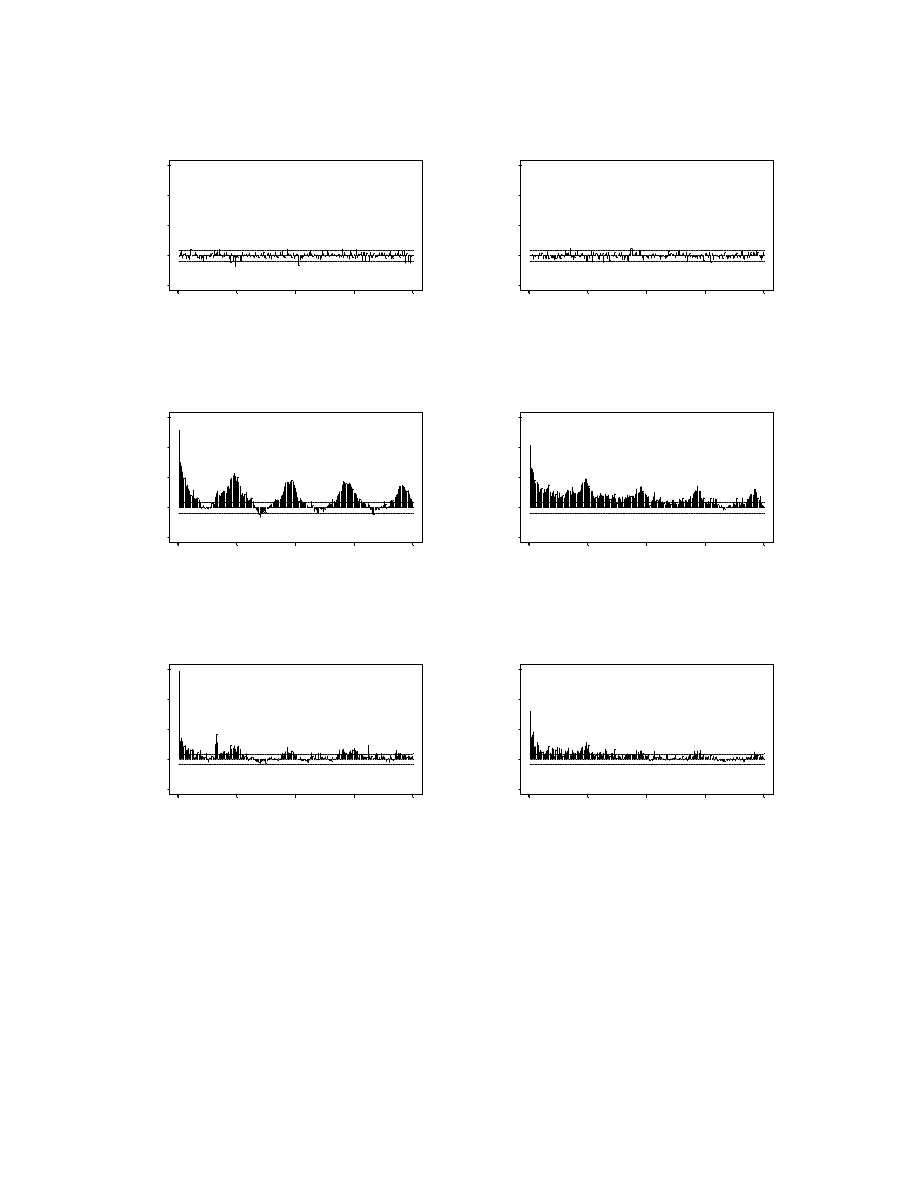
There are strong intra-day calendar effects in both Yen/$ and DM/$ returns; Figure 1

displays the first 200 autocorrelations of

. The calendar effects are particularly

pronounced in the absolute returns of both series; they occur because trading is more active at

certain times of day than at others. For instance, trading is much less active during the

Japanese lunch hour, and much more active when the U.S. markets open for trading. Figure

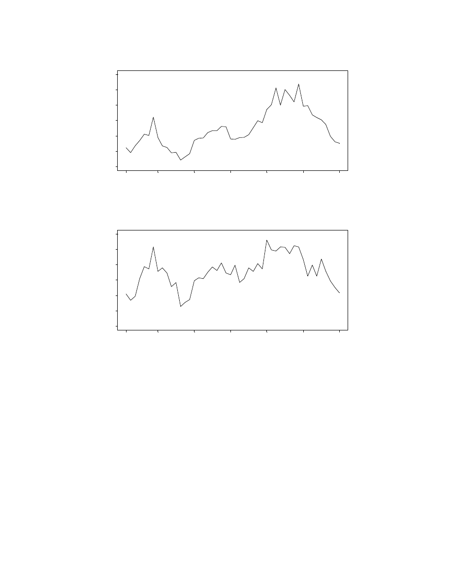
2, which plots volatility at the 48 half-hour intervals across an average day as measured by

mean absolute returns, clearly reveals these phenomena. The intra-day volatility pattern

corresponds closely to the pattern obtained by Andersen and Bollerslev (1997) for 5-minute

DM/$ returns.

As with the conditional mean of the returns process, intra-day calendar effects in

return volatility are not of primary concern to us; hence we remove them. Taking

where represents the “nonseasonal” portion of the process, we remove volatility calendar

effects by fitting time-of-day dummies to

. The F tests of no

time-of-day effects confirm that calendar effects are present in both series; the F(47, 12527)

statistics are 17.34 and 8.927 for the DM/$ and Yen/$ respectively and have zero p-values.

Suitably normalized so that

summed over the entire sample would be equal to one, we use

these time-of-day dummies to standardize the returns.

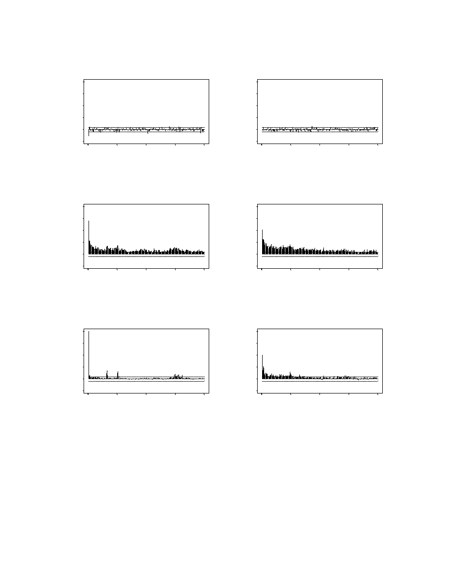
Figure 3 displays the autocorrelations of the levels, absolute and squared standardized

0
0

11, t| t 1

12, t| t 1

21, t| t 1

22, t| t 1

11, t| t 1

11, t 1| t 2

1, t 1

22, t| t 1

22, t 1| t 2

2, t 1

12, t| t 1

12, t 1| t 2

1, t 1

2, t 1

p(y

, y

)

p(y

) p(y

| y

)

p(y

, y

)

p(y

) p(y

| y

, z

2|1

, z

and z

1|2

returns of both currencies. The standardization removes the intraday calendar effects in

volatility, and as in Andersen and Bollerslev (1997), their removal highlights a feature of the

data that, at least in the case of the DM/$, was not obvious: the autocorrelations of absolute

returns decay very slowly.

Construction of Multivariate Density Forecasts

We construct density forecasts of the two exchange rates using the exponential

smoothing approach of RiskMetrics, which assumes that the returns are generated from a

multivariate normal distribution, yielding the bivariate density forecasts

where

and is the decay factor. RiskMetrics applies the same decay factor to each of the variances

and covariances, which ensures that the variance-covariance matrix is positive definite.

Density Forecast Evaluation

As discussed earlier, we evaluate the bivariate density forecasts generated by the

RiskMetrics approach decomposing the forecasts in two ways:

(i)

and

(ii)

t = 1, ..., T. We label the respective z series

, where we obtain by

p(y

)

i| j

p(y

| y

)

, z

2|1

, z

and z

1|2

0.95

, z

2|1

, z

and z

1|2

0.95

0.83

, z

2|1

, z

and z

1|2

taking the probability integral transform of with respect to

, and we obtain

transforming with respect to

. Good multivariate forecasts will produce

that are each iid U(0, 1).

To illustrate the multivariate density forecast evaluation procedures we split the

sample in two, the first running from January 1, 00:30 GMT to June 30, 21:00 GMT (6234

observations) and the second running from June 30, 21:30 GMT to December 31, 23:30 GMT

(6431 observations); we call them the “estimation sample” and the “forecast sample,”

respectively. We first evaluate forecasts generated using a decay factor of

, which is

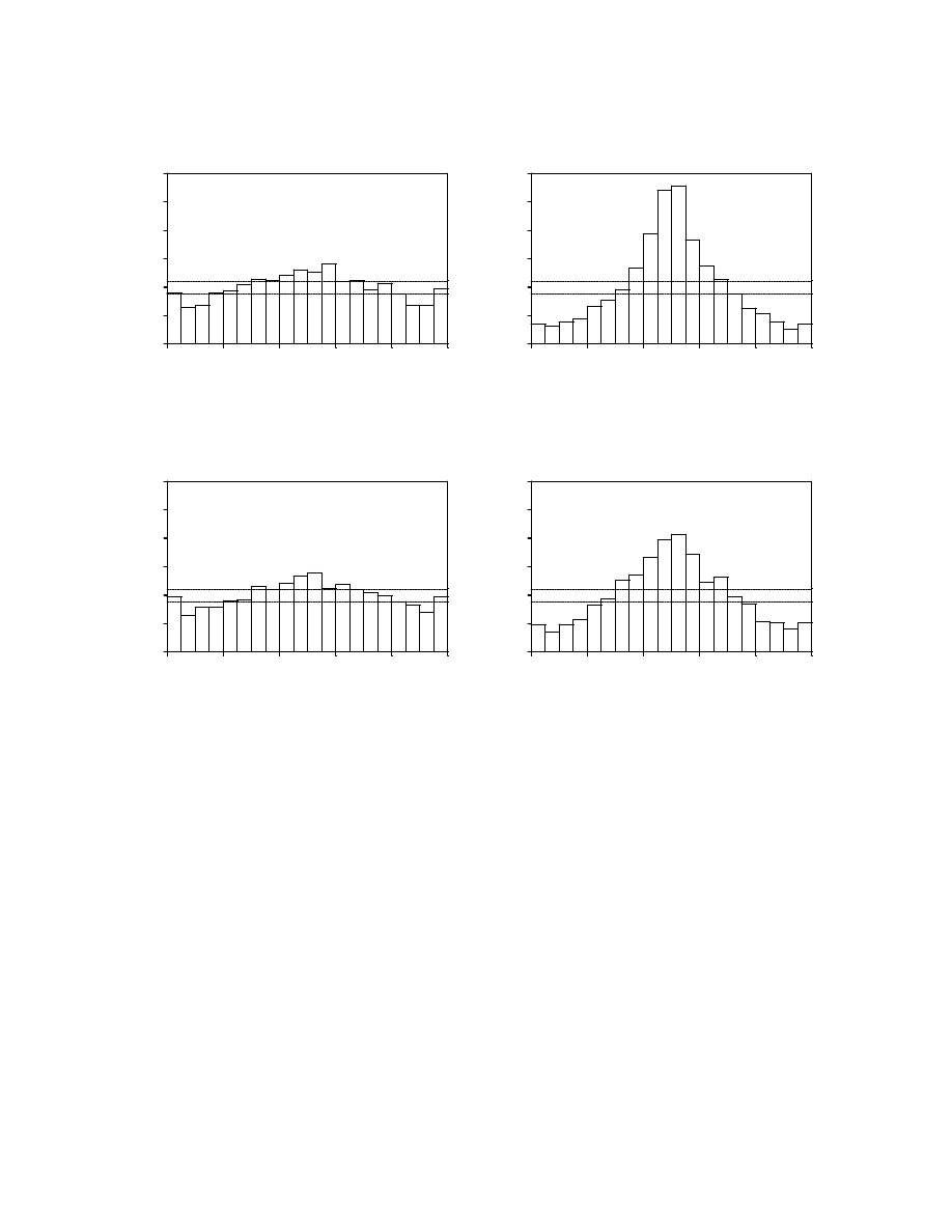
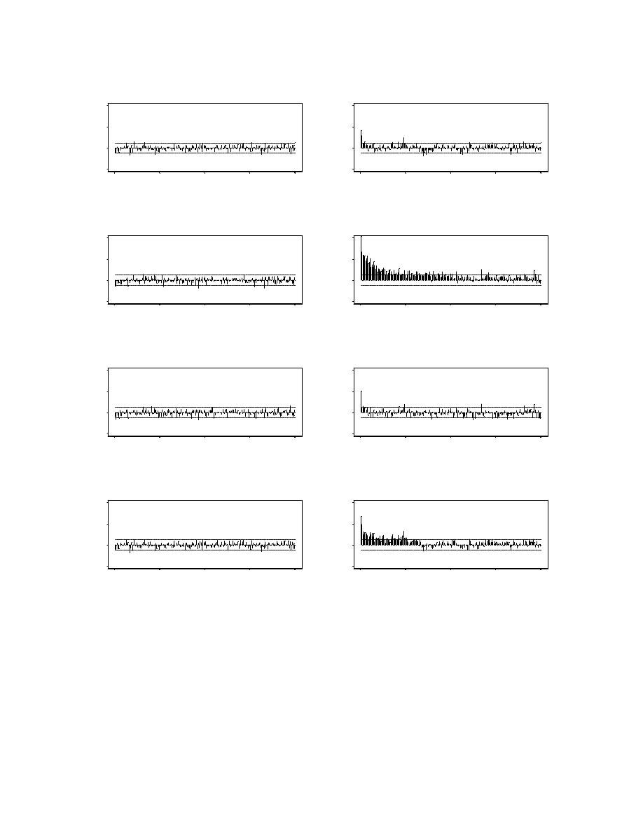
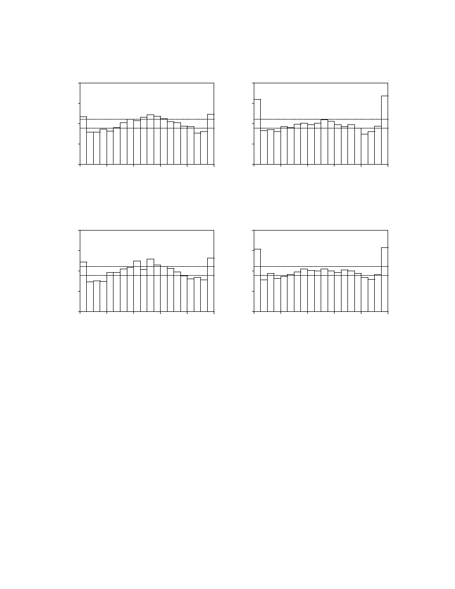
typical of RiskMetrics implementations. Figures 4a and 4b display the histograms and

correlograms of

; the histograms show clearly that the normality

assumption is inappropriate, and the correlograms show clearly that the decay factor

does not produce forecasts that capture the dynamics in return volatilities and correlations.

Although the correlograms of levels of z’s look fine, the correlograms of squares of z’s

indicate strong serial dependence. The positive serial correlation suggests that the decay

factor of 0.95 produces volatilities that adapt too slowly. Thus it appears that a smaller decay

factor would be appropriate.

We next turn to forecasts generated with an “optimal” decay factor, which we obtain

from the estimation sample as the decay factor that produced integral transforms that visually

appeared closest to iid, as assessed in our usual way, via correlograms of z and its powers. As

expected, a smaller decay factor (

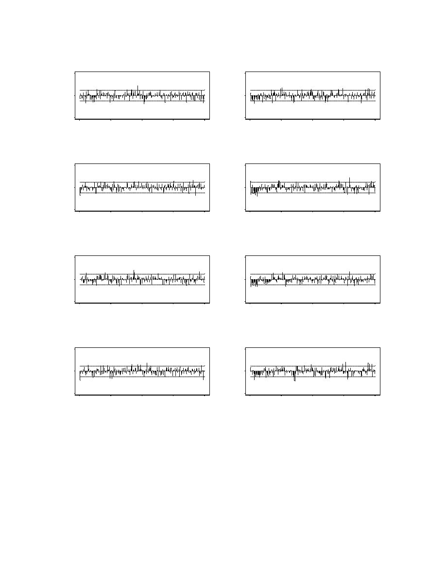
) turns out to be optimal. Figures 5a and 5b display

the histograms and correlograms of

and their squares, based on the

estimation sample, each with its mean removed before the correlograms are computed. The

ˆf(y

1,m 1

, y

2,m 1

,..., y

N,m 1

)

1,m 1

, y

2,m 1

,..., y

N,m 1

) ˆq(z

1,m 1

, z

2,m 1

,..., z

N,m 1

ˆF(y

1,m 1

,...,y

N,m 1

)

ˆQ(P

1,m 1

,...,y

N,m 1

)).

, z

2|1

, z

and z

1|2

, z

2|1

, z

and z

1|2

0.83

.83

ˆQ( )

correlograms indicate that the forecasts capture adequately the dynamics in return volatilities

and correlations (that is,

and their squares appear serially uncorrelated).

The histograms, in contrast, show clearly that the normality assumption is a poor one.

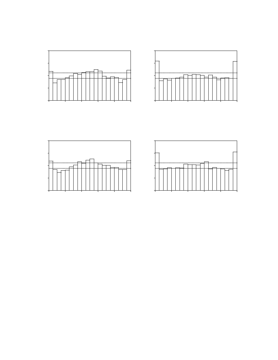
The smaller decay factor of 0.83 also produces much better out-of-sample joint

forecasts of the two exchange rate returns. Figures 6a and 6b display the histograms and

correlograms of

and their squares, based on the forecast sample,

corresponding to density forecasts produced using

. The histograms again show

clearly that the normality assumption is inadequate. The correlograms of squares, on the

other hand, all show clear improvement and indicate little, if any, serial correlation.

Density Forecast Calibration

We now attempt to improve the

RiskMetrics forecasts, which seemed to capture

dynamics adequately but which were plagued by an inappropriate normality assumption, by

calibrating. Recall that we use the transformation

or equivalently,

We obtain

from the z series based on the estimation sample. Although we favor the

presentation of histograms for density forecast evaluation, calibration is facilitated by using

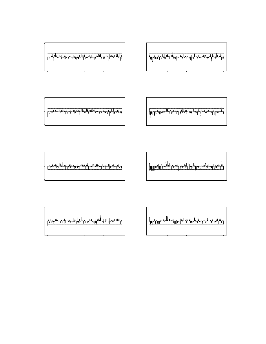
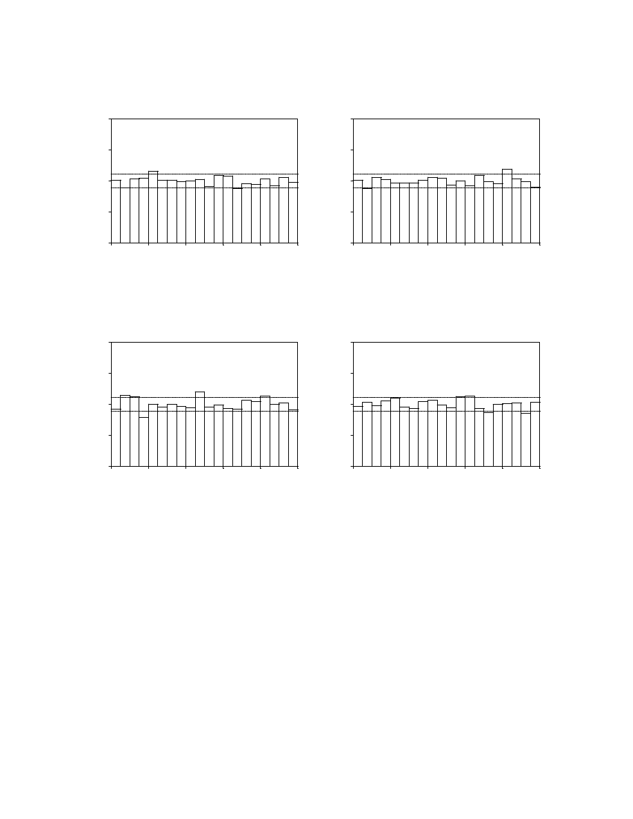
the empirical c.d.f. form. We present the histograms and correlograms of the four z series

corresponding to the calibrated forecasts in Figures 7a and 7b; clearly the histograms of the

calibrated forecasts are substantially improved relative to their non-calibrated counterparts,

and the correlograms remain good (that is, they are not affected by the calibration.)

5. Concluding Remarks and Directions for Future Research

We have proposed a framework for multivariate density forecast evaluation and

calibration. The multivariate forecast evaluation procedure is a generalization of the

univariate procedure proposed in Diebold, Gunther and Tay (1998) and shares its constructive

nature and ease of implementation. We illustrated the power of the procedure to detect and

remove defects in bivariate exchange rate density forecasts generated by a popular method.

An interesting direction for future research involves using recursive techniques for

real-time monitoring for breakdown of density forecast adequacy. Real-time monitoring

using CUSUM techniques is a simple matter in the univariate case, because under the

adequacy hypothesis the z series is iid U(0,1), which is free of nuisance parameters.

Appropriate boundary crossing probabilities for the CUSUM of the z series can be computed,

as in Chu, Stinchcombe and White (1996), using results on boundary crossing probabilities of

sample sums such as those of Robbins and Siegmund (1970). Multivariate CUSUM schemes

are also possible, as with the multivariate profile charts of Fuchs and Benjamini (1994).

References

Aït-Sahalia, Y. and A. Lo (1998), “Nonparametric Estimation of State-Price Densities Implicit

in Financial Asset Prices,” Journal of Finance, 53, 499-547.

Andersen, T.G. and Bollerslev, T. (1997), “Intraday Periodicity and Volatility Persistence in

Financial Markets,” Journal of Empirical Finance, 4, 115-158.

Bai, J. (1997), “Testing Parametric Conditional Distributions of Dynamic Models,”

Manuscript, Department of Economics, MIT.

Baillie, R.T. and Bollerslev, T. (1992), “Prediction in Dynamic Models with Time Dependent

Conditional Variances,” Journal of Econometrics, 52, 91-114.

Bollerslev, T., Engle, R.F. and Nelson, D. (1994), “ARCH Models,” in R.F. Engle and D.L.

McFadden (eds.), Handbook of Econometrics, Volume 4. Amsterdam: North-

Holland.

Bollerslev, T. and Wooldridge, J.M. (1992), “Quasi-Maximum Likelihood Estimation and

Inference in Dynamic Models with Time-Varying Covariances,” Econometric
Reviews

, 11, 143-179.

Brock, W.A., Hsieh, D.A. and LeBaron, B. (1991), Nonlinear Dynamics, Chaos, and

Instability

. Cambridge, Mass.: MIT Press.

Campa, J.M., Chang, P.H.K. and Reider, R.L. (1998), “Implied Exchange Rate Distributions:

Evidence From OTC Markets,” Journal of International Money and Finance, 17, 117-

160.

Chatfield, C. (1993), “Calculating Interval Forecasts,” Journal of Business and Economics

Statistics

, 11, 121-135.

Christoffersen, P.F. (1998), “Evaluating Interval Forecasts,” International Economic Review,

39, forthcoming.

Chu, C.-S. J., Stinchcombe, M. and White, H. (1996), “Monitoring Structural Change,”

Econometrica

, 64, 1045-1065.

Clements, M.P. and Smith, J. (1998), “Evaluating the Forecast Densities of Linear and Non-

Linear Models: Applications to Output Growth and Unemployment,” Manuscript,

University of Warwick.

Dawid, A.P. (1984), “Statistical Theory: The Prequential Approach,” Journal of the Royal

Statistical Society

, Series A, 147, 278-292.

Diebold, F.X. and Lopez, J. (1996), “Forecast Evaluation and Combination,” in G.S. Maddala

and C.R. Rao (eds.), Statistical Methods in Finance (Handbook of Statistics, Volume

14). Amsterdam: North-Holland, 241-268.

Diebold, F.X., Gunther, T. and Tay, A.S. (1998), “Evaluating Density Forecasts, with

Applications to Financial Risk Management,” International Economic Review, 39,

forthcoming.

Diebold, F.X., Tay, A.S. and Wallis, K.F. (1997), “Evaluating Density Forecasts of Inflation:

The Survey of Professional Forecasters,” NBER Working Paper 6228. Forthcoming

in R. Engle and H. White (eds.), Festschrift in Honor of C.W.J. Granger.

Duan, J.-C. (1995), “The GARCH Options Pricing Model,” Mathematical Finance, 5, 13-32.

Duan, J.-C., Gauthier, G. and Simonato, J.-G. (1997), “An Analytical Approximation for the

GARCH Option Pricing Model,” Manuscript, Hong Kong University of Science and

Technology.

Duffie, D. and Pan, J. (1997), “An Overview of Value at Risk,” Journal of Derivatives, 4, 7-

49.

Engle, R.F. and González-Rivera, G. (1991), “Semiparametric ARCH Models,” Journal of

Business and Economic Statistics

, 9, 345-359.

Fackler, P.L. and King, R.P. (1990), “Calibration of Options-Based Probability Assessments

in Agricultural Commodity Markets,” American Journal of Agricultural Economics,

72, 73-83.

Fuchs, C. and Benjamini, Y. (1994), “Multivariate Profile Charts for Statistical Process

Control,” Technometrics, 36, 182-195.

Gelman, A, Carlin, J.B., Stern, H.S. and Rubin, D.B. (1995), Bayesian Data Analysis.

London: Chapman and Hall.

Ghysels, E., Harvey, A. and Renault, E. (1996), “Stochastic Volatility,” in G.S. Maddala and

C.R. Rao (eds.), Statistical Methods in Finance (Handbook of Statistics, Volume 14).

Amsterdam: North-Holland.

Hansen, B.E. (1994), “Autoregressive Conditional Density Estimation,” International

Economic Review

, 35, 705-730.

Härdle, W. (1990), Applied Nonparametric Regression. Cambridge: Cambridge University

Press.

Härdle, W. (1991), Smoothing Techniques. New York: Springer-Verlag.

Harrison, P.J. and Stevens, C. (1976), “Bayesian Forecasting” (with discussion), Journal of

the Royal Statistical Society B

, 38, 205-247.

Inoue, A. (1997), “A Conditional Goodness-of-Fit Test for Time Series,” Manuscript,

Department of Economics, University of Pennsylvania.

Jorion, P. (1997), Value at Risk. San Diego: Academic Press.

JP Morgan (1996), “RiskMetrics --Technical Document,” Fourth Edition, New York.

Mincer, J. and V. Zarnowitz (1969), “The Evaluation of Economic Forecasts,” in J. Mincer

(ed.), Economic Forecasts and Expectations. New York: National Bureau of

Economic Research.

Morvai, G., Yakowitz, S.J. and Algoet, P. (1997), “Weakly Convergent Nonparametric

Forecasting of Stationary Time Series,” IEEE Transactions on Information Theory, 43,

483-498.

Müller, H.-G. (1993), “On the Boundary Kernel Method for Nonparametric Curve Estimation

Near End Points,” Scandinavian Journal of Statistics, 20, 313-328.

Robbins, H. and Siegmund, D. (1970), “Boundary Crossing Probabilities for the Wiener

Process and Sample Sums,” Annals of Mathematical Statistics, 41, 1410-1429.

Rosenblatt, M. (1952), “Remarks on a Multivariate Transformation,” Annals of Mathematical

Statistics

, 23, 470-472.

Seillier-Moiseiwitsch, F. (1993), “Sequential Probability Forecasts and the Probability

Integral Transform,” International Statistical Review, 61, 395-408.

Shephard, N. (1994), “Partial Non-Gaussian State Space,” Biometrika, 81, 115-131.

Silverman, B.W. (1986), Density Estimation for Statistics and Data Analysis. New York:

Chapman and Hall.

Soderlind, P. and Svensson, L.E.O. (1997), “New Techniques to Extract Market Expectations

from Financial Instruments,” National Bureau of Economic Research Working Paper

5877, Cambridge, Mass.

West, M. and Harrison, P.J. (1997), Bayesian Forecasting and Dynamic Models (Second

Edition). New York: Springer-Verlag.

100

150

200

-0.1

0.0

0.1

0.2

0.3

100

150

200

100

150

200

(a) DM / $

100

150

200

100

150

200

100

150

200

-0.1

0.0

0.1

0.2

0.3

(b) YEN / $

100

150

200

100

150

200

100

150

200

-0.1

0.0

0.1

0.2

0.3

100

150

200

100

150

200

100

150

200

-0.1

0.0

0.1

0.2

0.3

(d) YEN / $ (abs)

100

150

200

100

150

200

100

150

200

-0.1

0.0

0.1

0.2

0.3

(e) DM / $ (sq)

100

150

200

100

150

200

100

150

200

-0.1

0.0

0.1

0.2

0.3

(f) YEN / $ (sq)

Figure 1

A.c.f.s of Returns, Absolute Returns and Squared Returns

MA(1) Component Removed

0.02

0.03

0.04

0.05

0.06

0.07

0.08

2130 0100

0500

0900

1300

1700

2100

GMT

DM / $

0.02

0.03

0.04

0.05

0.06

0.07

0.08

2130 0100

0500

0900

1300

1700

2100

GMT

YEN / $

Figure 2

Mean Intraday Absolute Returns

100

150

200

-0.1

0.0

0.1

0.2

0.3

0.4

100

150

200

100

150

200

(a) DM / $

100

150

200

100

150

200

100

150

200

-0.1

0.0

0.1

0.2

0.3

0.4

(b) YEN / $

100

150

200

100

150

200

100

150

200

-0.1

0.0

0.1

0.2

0.3

0.4

100

150

200

100

150

200

100

150

200

-0.1

0.0

0.1

0.2

0.3

0.4

(d) YEN / $ (abs)

100

150

200

100

150

200

100

150

200

-0.1

0.0

0.1

0.2

0.3

0.4

(e) DM / $ (sq)

100

150

200

100

150

200

100

150

200

-0.1

0.0

0.1

0.2

0.3

0.4

(f) YEN / $ (sq)

Figure 3

A.c.f.s of Returns, Absolute Returns and Squared Returns

Conditional Mean MA(1) Component Removed

Volatility Intra-Day Calendar Effects Removed

0.0

0.2

0.4

0.6

0.8

1.0

0.0

1.0

2.0

3.0

0.0

0.2

0.4

0.6

0.8

1.0

0.0

1.0

2.0

3.0

0.0

0.2

0.4

0.6

0.8

1.0

0.0

1.0

2.0

3.0

(i) z1

0.0

0.2

0.4

0.6

0.8

1.0

0.0

1.0

2.0

3.0

0.0

0.2

0.4

0.6

0.8

1.0

0.0

1.0

2.0

3.0

0.0

0.2

0.4

0.6

0.8

1.0

0.0

1.0

2.0

3.0

(ii) z2|1

0.0

0.2

0.4

0.6

0.8

1.0

0.0

1.0

2.0

3.0

0.0

0.2

0.4

0.6

0.8

1.0

0.0

1.0

2.0

3.0

0.0

0.2

0.4

0.6

0.8

1.0

0.0

1.0

2.0

3.0

(iii) z2

0.0

0.2

0.4

0.6

0.8

1.0

0.0

1.0

2.0

3.0

0.0

0.2

0.4

0.6

0.8

1.0

0.0

1.0

2.0

3.0

0.0

0.2

0.4

0.6

0.8

1.0

0.0

1.0

2.0

3.0

(iv) z1|2

Figure 4a

Histograms of z (decay factor=0.95, forecast sample)

100

150

200

-0.1

0.0

0.1

0.2

100

150

200

100

150

200

-0.1

0.0

0.1

0.2

(i) z1

100

150

200

-0.1

0.0

0.1

0.2

100

150

200

100

150

200

-0.1

0.0

0.1

0.2

(ii) z1 (square)

100

150

200

-0.1

0.0

0.1

0.2

100

150

200

100

150

200

-0.1

0.0

0.1

0.2

(iii) z2|1

100

150

200

-0.1

0.0

0.1

0.2

100

150

200

100

150

200

-0.1

0.0

0.1

0.2

(iv) z2|1 (square)

100

150

200

-0.1

0.0

0.1

0.2

100

150

200

100

150

200

-0.1

0.0

0.1

0.2

(v) z2

100

150

200

-0.1

0.0

0.1

0.2

100

150

200

100

150

200

-0.1

0.0

0.1

0.2

(vi) z2 (square)

100

150

200

-0.1

0.0

0.1

0.2

100

150

200

100

150

200

-0.1

0.0

0.1

0.2

(vii) z1|2

100

150

200

-0.1

0.0

0.1

0.2

100

150

200

100

150

200

-0.1

0.0

0.1

0.2

(viii) z1|2 (square)

Figure 4b

Correlograms of powers of z (decay factor=0.95, forecast sample)

0.0

0.2

0.4

0.6

0.8

1.0

0.0

1.0

2.0

0.0

0.2

0.4

0.6

0.8

1.0

0.0

1.0

2.0

0.0

0.2

0.4

0.6

0.8

1.0

0.0

1.0

2.0

(i) z1

0.0

0.2

0.4

0.6

0.8

1.0

0.0

1.0

2.0

0.0

0.2

0.4

0.6

0.8

1.0

0.0

1.0

2.0

0.0

0.2

0.4

0.6

0.8

1.0

0.0

1.0

2.0

(ii) z2|1

0.0

0.2

0.4

0.6

0.8

1.0

0.0

1.0

2.0

0.0

0.2

0.4

0.6

0.8

1.0

0.0

1.0

2.0

0.0

0.2

0.4

0.6

0.8

1.0

0.0

1.0

2.0

(iii) z2

0.0

0.2

0.4

0.6

0.8

1.0

0.0

1.0

2.0

0.0

0.2

0.4

0.6

0.8

1.0

0.0

1.0

2.0

0.0

0.2

0.4

0.6

0.8

1.0

0.0

1.0

2.0

(iv) z1|2

Figure 5a

Histograms of z (decay factor=0.83, estimation sample)

100

150

200

-0.1

0.0

0.1

100

150

200

100

150

200

-0.1

0.0

0.1

(i) z1

100

150

200

100

150

200

100

150

200

-0.1

0.0

0.1

(ii) z1 (square)

100

150

200

100

150

200

100

150

200

-0.1

0.0

0.1

(iii) z2|1

100

150

200

100

150

200

100

150

200

-0.1

0.0

0.1

(iv) z2|1 (square)

100

150

200

-0.1

0.0

0.1

100

150

200

100

150

200

-0.1

0.0

0.1

(v) z2

100

150

200

100

150

200

100

150

200

-0.1

0.0

0.1

(vi) z2 (square)

100

150

200

100

150

200

100

150

200

-0.1

0.0

0.1

(vii) z1|2

100

150

200

100

150

200

100

150

200

-0.1

0.0

0.1

(viii) z1|2 (square)

Figure 5b

Correlograms of powers of z (decay factor=0.83, estimation sample)

0.0

0.2

0.4

0.6

0.8

1.0

0.0

1.0

2.0

0.0

0.2

0.4

0.6

0.8

1.0

0.0

1.0

2.0

0.0

0.2

0.4

0.6

0.8

1.0

0.0

1.0

2.0

(i) z1

0.0

0.2

0.4

0.6

0.8

1.0

0.0

1.0

2.0

0.0

0.2

0.4

0.6

0.8

1.0

0.0

1.0

2.0

0.0

0.2

0.4

0.6

0.8

1.0

0.0

1.0

2.0

(ii) z2|1

0.0

0.2

0.4

0.6

0.8

1.0

0.0

1.0

2.0

0.0

0.2

0.4

0.6

0.8

1.0

0.0

1.0

2.0

0.0

0.2

0.4

0.6

0.8

1.0

0.0

1.0

2.0

(iii) z2

0.0

0.2

0.4

0.6

0.8

1.0

0.0

1.0

2.0

0.0

0.2

0.4

0.6

0.8

1.0

0.0

1.0

2.0

0.0

0.2

0.4

0.6

0.8

1.0

0.0

1.0

2.0

(iv) z1|2

Figure 6a

Histograms of z (decay factor=0.83, forecast sample)

100

150

200

-0.1

0.0

0.1

100

150

200

100

150

200

-0.1

0.0

0.1

(i) z1

100

150

200

-0.1

0.0

0.1

100

150

200

100

150

200

-0.1

0.0

0.1

(ii) z1 (square)

100

150

200

-0.1

0.0

0.1

100

150

200

100

150

200

-0.1

0.0

0.1

(iii) z2|1

100

150

200

-0.1

0.0

0.1

100

150

200

100

150

200

-0.1

0.0

0.1

(iv) z2|1 (square)

100

150

200

-0.1

0.0

0.1

100

150

200

100

150

200

-0.1

0.0

0.1

(v) z2

100

150

200

-0.1

0.0

0.1

100

150

200

100

150

200

-0.1

0.0

0.1

(vi) z2 (square)

100

150

200

-0.1

0.0

0.1

100

150

200

100

150

200

-0.1

0.0

0.1

(vii) z1|2

100

150

200

-0.1

0.0

0.1

100

150

200

100

150

200

-0.1

0.0

0.1

(viii) z1|2 (square)

Figure 6b

Correlograms of powers of z (decay factor=0.83, forecast sample)

0.0

0.2

0.4

0.6

0.8

1.0

0.0

1.0

2.0

0.0

0.2

0.4

0.6

0.8

1.0

0.0

1.0

2.0

0.0

0.2

0.4

0.6

0.8

1.0

0.0

1.0

2.0

(i) z1

0.0

0.2

0.4

0.6

0.8

1.0

0.0

1.0

2.0

0.0

0.2

0.4

0.6

0.8

1.0

0.0

1.0

2.0

0.0

0.2

0.4

0.6

0.8

1.0

0.0

1.0

2.0

(ii) z2|1

0.0

0.2

0.4

0.6

0.8

1.0

0.0

1.0

2.0

0.0

0.2

0.4

0.6

0.8

1.0

0.0

1.0

2.0

0.0

0.2

0.4

0.6

0.8

1.0

0.0

1.0

2.0

(iii) z2

0.0

0.2

0.4

0.6

0.8

1.0

0.0

1.0

2.0

0.0

0.2

0.4

0.6

0.8

1.0

0.0

1.0

2.0

0.0

0.2

0.4

0.6

0.8

1.0

0.0

1.0

2.0

(iv) z1|2

Figure 7a

Histograms of z (decay factor=0.83, forecast sample, calibrated)

100

150

200

-0.1

0.0

0.1

100

150

200

100

150

200

-0.1

0.0

0.1

(i) z1

100

150

200

-0.1

0.0

0.1

100

150

200

100

150

200

-0.1

0.0

0.1

(ii) z1 (square)

100

150

200

-0.1

0.0

0.1

100

150

200

100

150

200

-0.1

0.0

0.1

(iii) z2|1

100

150

200

-0.1

0.0

0.1

100

150

200

100

150

200

-0.1

0.0

0.1

(iv) z2|1 (square)

100

150

200

-0.1

0.0

0.1

100

150

200

100

150

200

-0.1

0.0

0.1

(v) z2

100

150

200

-0.1

0.0

0.1

100

150

200

100

150

200

-0.1

0.0

0.1

(vi) z2 (square)

100

150

200

-0.1

0.0

0.1

100

150

200

100

150

200

-0.1

0.0

0.1

(vii) z1|2

100

150

200

-0.1

0.0

0.1

100

150

200

100

150

200

-0.1

0.0

0.1

(viii) z1|2 (square)

Figure 7b

Correlograms of powers of z (decay factor=0.83, forecast sample, calibrated)

Wyszukiwarka

Podobne podstrony:
1The effects of hybridization on the abundance of parental taxa depends on their relative frequency
Gallup Balkan Monitor The Impact Of Migration
THE IMPACT OF SOCIAL NETWORK SITES ON INTERCULTURAL COMMUNICATION
Orzeczenia, dyrektywa 200438, DIRECTIVE 2004/58/EC OF THE EUROPEAN PARLIAMENT AND OF THE COUNCIL of
5 The importance of memory and personality on students' success
Gallup Balkan Monitor The Impact Of Migration
Glińska, Sława i inni The effect of EDTA and EDDS on lead uptake and localization in hydroponically
Understanding the effect of violent video games on violent crime S Cunningham , B Engelstätter, M R
The Effect of Childhood Sexual Abuse on Psychosexual Functioning During Adullthood
Describe the role of the dental nurse in minimising the risk of cross infection during and after the
Jóźwiak, Małgorzata; Warczakowska, Agnieszka Effect of base–acid properties of the mixtures of wate
Conrad Hjalmar Nordby The Influence Of Old Norse Literature On English Literature
Marina Post The impact of Jose Ortega y Gassets on European integration
Microwave drying characteristics of potato and the effect of different microwave powers on the dried
The Impact of Mary Stewart s Execution on Anglo Scottish Relations
FALLS, INJURIES DUE TO FALLS, AND THE RISK OF ADMISSION
Brzechczyn, Krzysztof In the Trap of Post Socialist Stagnation On Political Development of the Bela
US Patent 577,670 Apparatus For Producing Electric Currents Of High Frequency

więcej podobnych podstron