CFX Intro 14 0 L11 Transient

January 16, 2012

Release 14.0

14. 0 Release

Introduction to ANSYS
CFX

Lecture 11
Transient Flows

January 16, 2012

Release 14.0

Introduction

•

Lecture Theme:

–

Performing a transient calculation is in some ways similar to performing a steady
state calculation, but there are additional considerations. More data is generated
and extra inputs are required. This lecture will explain these inputs and describe
transient data post‐processing

•

Learning Aims – you will learn:

–

How to set up and run transient calculations

–

How to choose the appropriate time step size for your calculation

–

How to post‐process transient data and make animations

•

Learning Objectives:

–

Transient flow calculations are becoming increasingly common due to advances in
high performance computing (HPC) and reductions in hardware costs. You will
understand what transient calculations involve and be able to perform them with
confidence

Introduction

Initialization

Solver

Output File

Summary

January 16, 2012

Release 14.0

Outline

•

Motivation

•

Setup

•

Time step estimation

•

Output

Introduction

Motivation

Setup

Time Steps

Output

January 16, 2012

Release 14.0

Motivation

•

Nearly all flows in nature are transient!

–

Steady‐state assumption is possible if we:
• Ignore unsteady fluctuations
• Employ ensemble/time‐averaging to remove unsteadiness (this is what is done

in modeling turbulence)

•

In CFD, steady‐state methods are preferred

–

Lower computational cost

–

Easier to postprocess and analyze

•

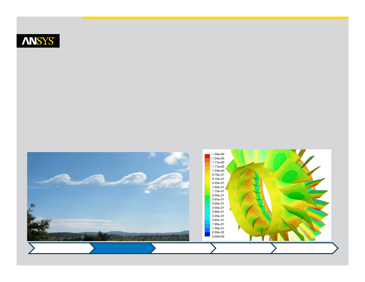
Many applications require resolution of transient flow:

–

Aerodynamics (aircraft, land vehicles,etc.) – vortex shedding

–

Rotating Machinery – rotor/stator interaction, stall, surge

–

Multiphase Flows – free surfaces, bubble dynamics

–

Deforming Domains – in‐cylinder combustion, store separation

–

Unsteady Heat Transfer – transient heating and cooling

–

Many more

Introduction

Motivation

Setup

Time Steps

Output

January 16, 2012

Release 14.0

Origins of Transient Flow

•

Natural unsteadiness

–

Unsteady flow due to growth of instabilities within the fluid or a non‐equilibrium
initial fluid state

–

Examples: natural convection flows, turbulent eddies of all scales, fluid waves
(gravity waves, shock waves)

•

Forced unsteadiness

–

Time‐dependent boundary conditions, source terms drive the unsteady flow field

–

Examples: pulsing flow in a nozzle, rotor‐stator interaction in a turbine stage

Introduction

Motivation

Setup

Time Steps

Output

January 16, 2012

Release 14.0

Transient CFD Analysis

•

Simulate a transient flow field over a specified time period

–

Solution may approach:
• Steady‐state solution – Flow variables stop changing with time
• Time‐periodic solution – Flow variables fluctuate with repeating pattern

–

Your goal may also be simply to analyze the flow over a prescribed time interval.
• Free surface flows
• Moving shock waves
• Etc.

•

Extract quantities of interest

–

Natural frequencies (e.g. Strouhal Number)

–

Time‐averaged and/or RMS values

–

Time‐related parameters (e.g. time required to cool a hot solid, residence time of
a pollutant)

–

Spectral data – fast Fourier transform (FFT)

Introduction

Motivation

Setup

Time Steps

Output

January 16, 2012

Release 14.0

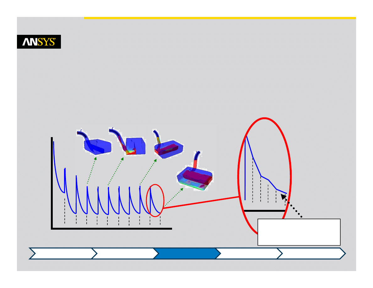
How to Solve a Transient Case

•

Transient simulations are solved by
computing a solution for many
discrete points in time

•

At each time point we must iterate
to the solution

Timestep = 2 s

Initial Time = 0 s

Total Time = 20 s

Coefficient Loops = 5

4 6 8 10 12 14 16 18

Time (seconds)

5 coefficient
Loops

Introduction

Motivation

Setup

Time Steps

Output

January 16, 2012

Release 14.0

How to Solve a Transient Case

•

Similar setup to steady state

•

The general workflow is:

–

Set the Analysis Type to Transient

–

Specify the transient time duration to solve and the time step size

–

Set up physical models and boundary conditions as usual
• Boundary conditions may change with time

–

Prescribe initial conditions
• Best to use a physically realistic initial condition, such as a steady solution

–

Assign solver settings

–

Configure transient results files, transient statistics, monitor points

–

Run the solver

Introduction

Motivation

Setup

Time Steps

Output

January 16, 2012

Release 14.0

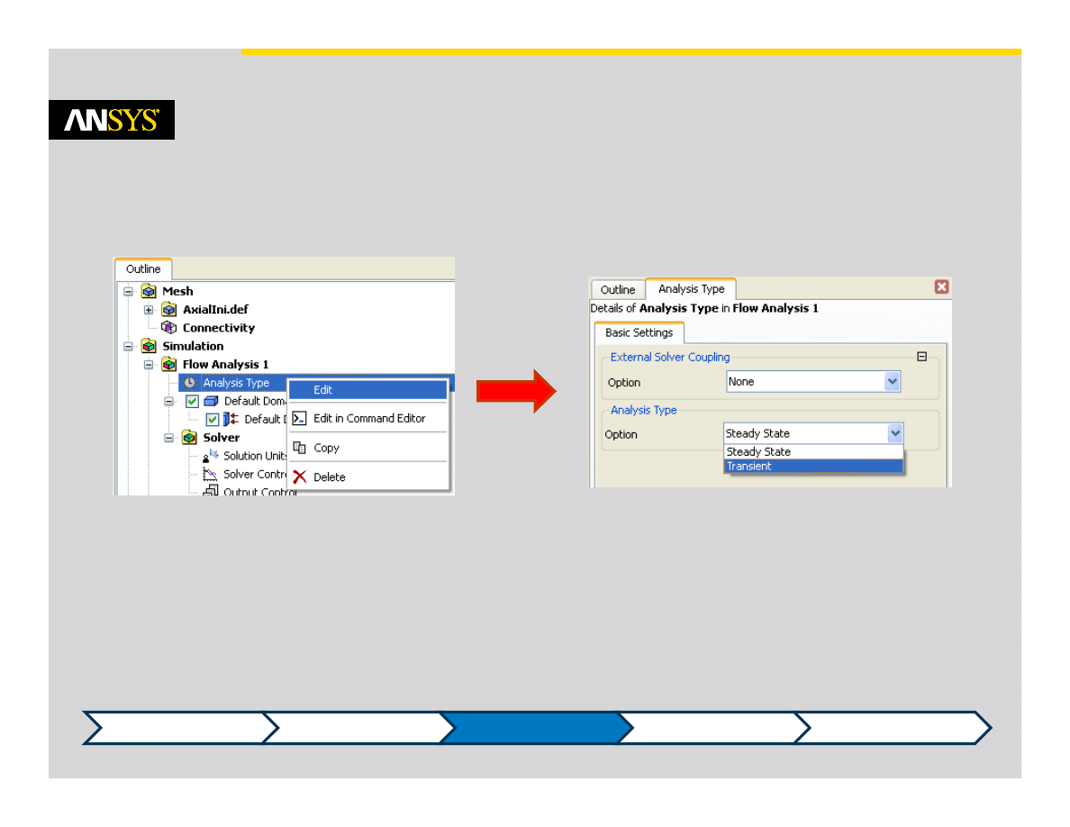
Analysis Type

•

Edit ‘Analysis Type’ in the Outline tree and set the Option to ‘Transient’

Introduction

Motivation

Setup

Time Steps

Output

January 16, 2012

Release 14.0

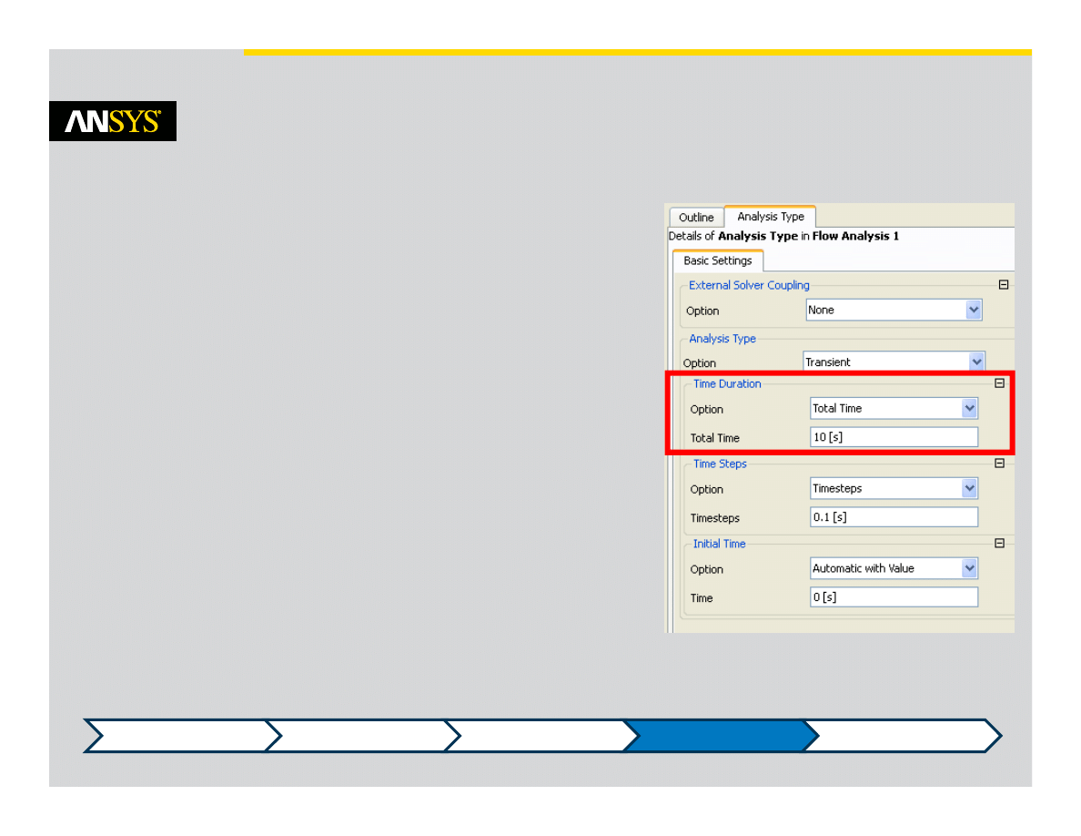
Time Duration and Time Step

•

Set the Time Duration

–

This controls when the simulation will end

•

Options are:

–

Total Time
• When restarting, this time carries over

–

Time per Run
• Ignores any time completed in previous runs

–

Maximum number of Timesteps
• The number of timesteps to perform, including

any completed in previous runs

–

Number of Timesteps per Run
• For this run only. Ignores previously completed

timesteps

Introduction

Motivation

Setup

Time Steps

Output

January 16, 2012

Release 14.0

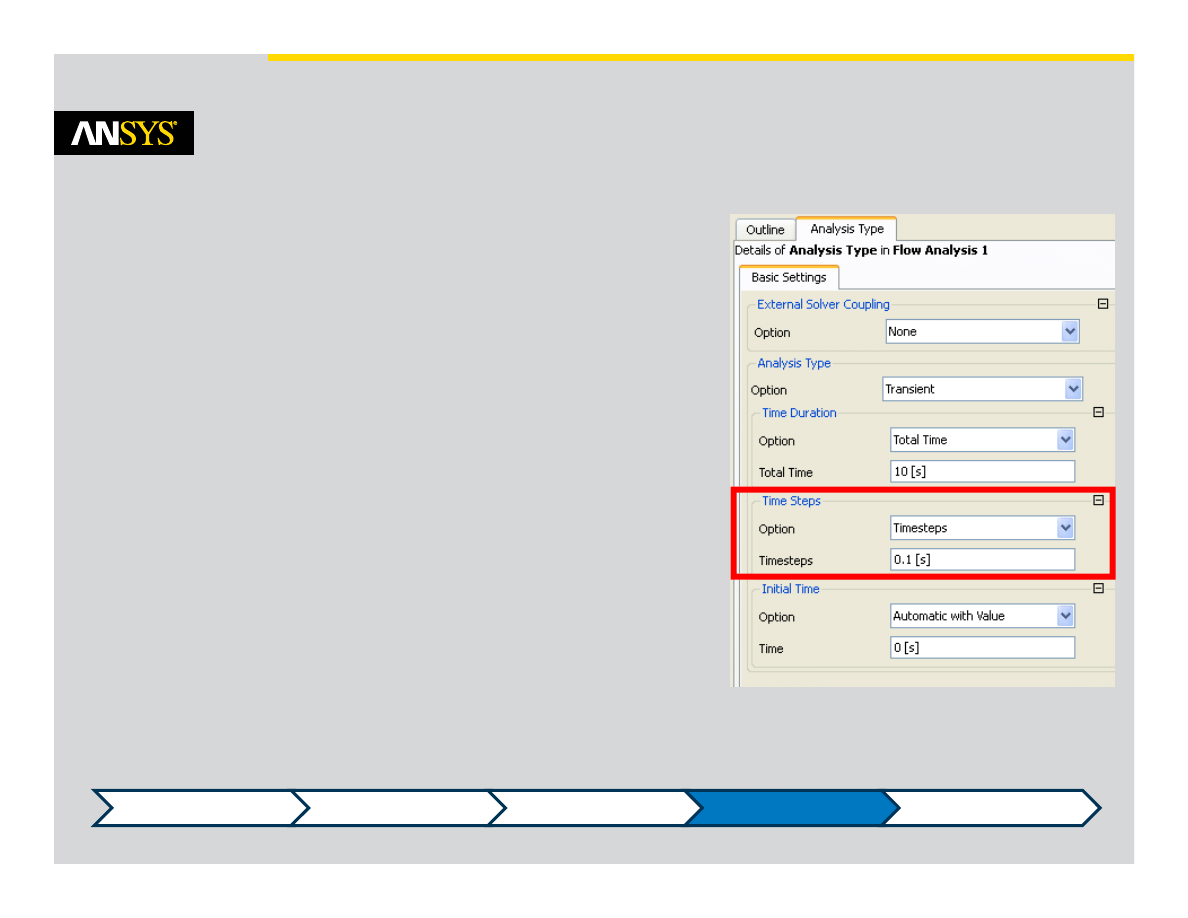
Time Duration and Time Step

•

Set the Time Step size

–

This controls the spacing in time between the
solutions points

•

Options are:

–

Timesteps / Timesteps for the Run
• Various formats accepted, e.g.
• 0.001
• 0.001, 0.002, 0.002, 0.003
• 5*0.001, 10*0.05, 20*0.06

–

Adaptive
• Timestep size will change dynamically within

specified limits depending on specified
convergence criteria or Courant number

Introduction

Motivation

Setup

Time Steps

Output

January 16, 2012

Release 14.0

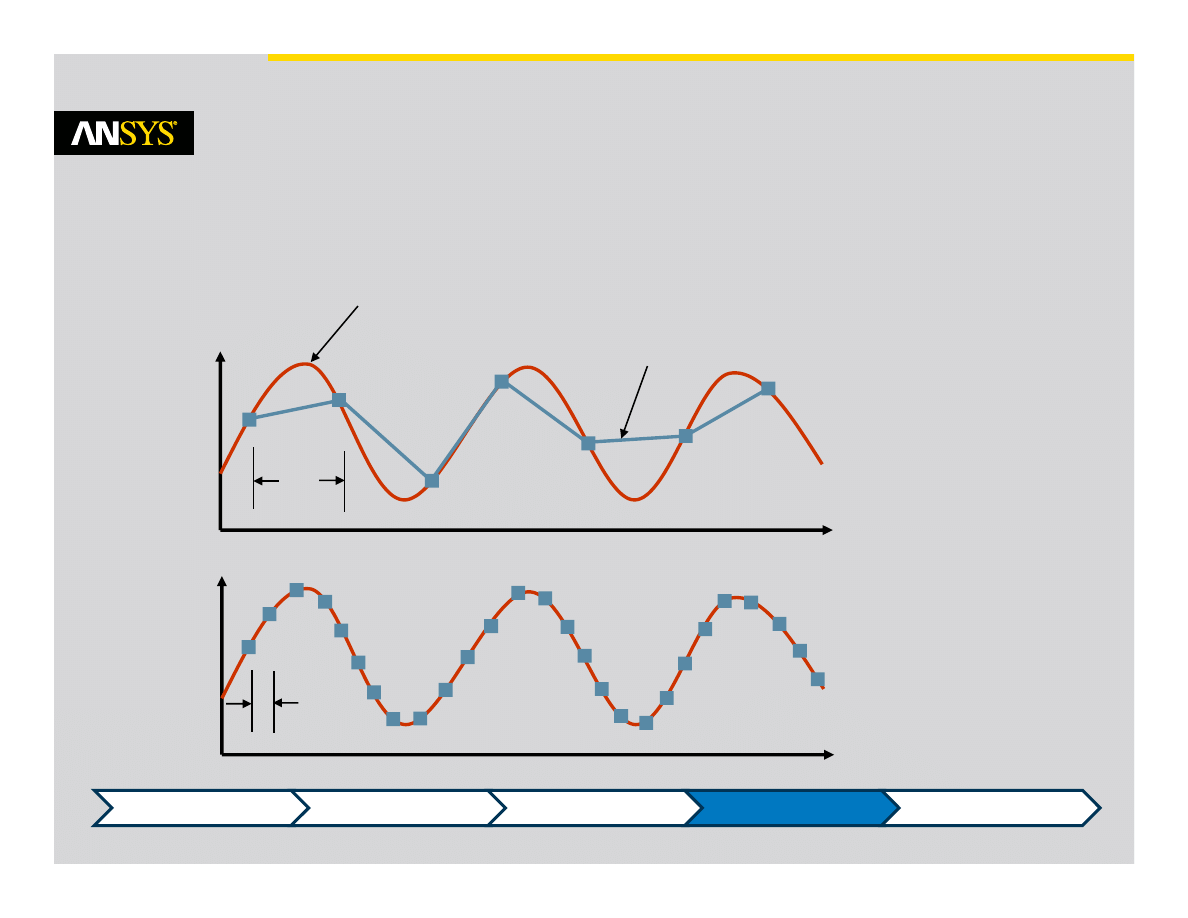
Time Duration and Time Step

•

The Time Step size is an important parameter in transient simulations

–

It must be small enough to resolve time‐dependent features

True solution

Time

Variable of
interest

t

Time

Variable of
interest

t

Time step too large to resolve transient
changes. Note the solution points generally
will not lie on the true solution because the
true behaviour has not been resolved.

A smaller time step can
resolve the true solution

Introduction

Motivation

Setup

Time Steps

Output

January 16, 2012

Release 14.0

Time Duration and Time Step

•

…and it must be small enough to maintain solver stability

–

The quantity of interest may be changing very slowly (e.g. temperature in a solid),
but you may not be able to use a large timestep if other quantities (e.g. velocity)
have smaller timescales

•

The Courant Number is often used to estimate a time step:

–

This gives the number of mesh elements the fluid passes through in one timestep

–

Typical values are 2 – 10, but in some cases higher values are acceptable

–

The average and maximum Courant number is reported in the Solver out file each
timestep

•

A smaller timestep will typically improve convergence

Size

Element

Velocity

Number

Courant







Introduction

Motivation

Setup

Time Steps

Output

January 16, 2012

Release 14.0

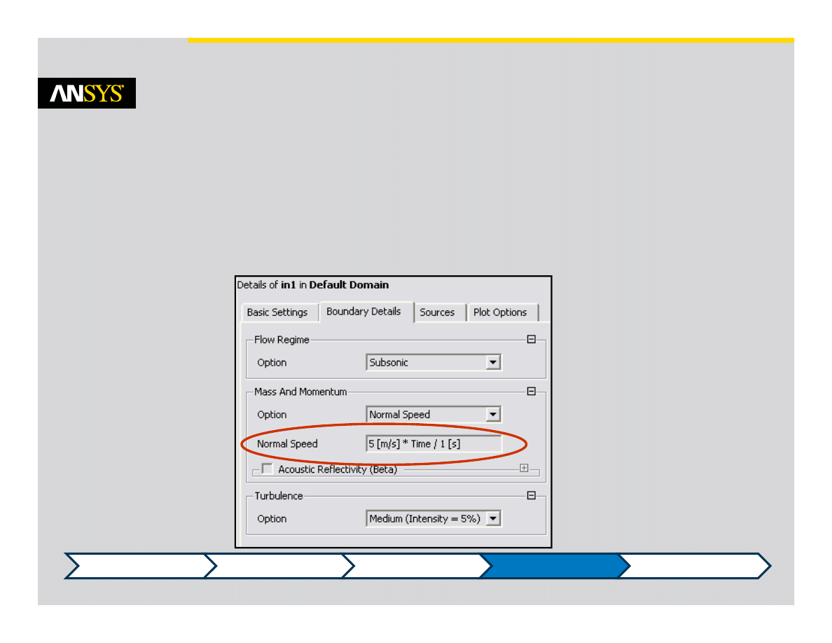
Boundary Conditions

•

If required, boundary conditions can be functions of time instead of constant
values

–

Velocities, Mass flows, pressure conditions, temperatures, etc. can all be expressed
as functions

–

In CEL expressions use “t” or “Time”

–

Can read in time varying experimental data through User FORTRAN

Introduction

Motivation

Setup

Time Steps

Output

January 16, 2012

Release 14.0

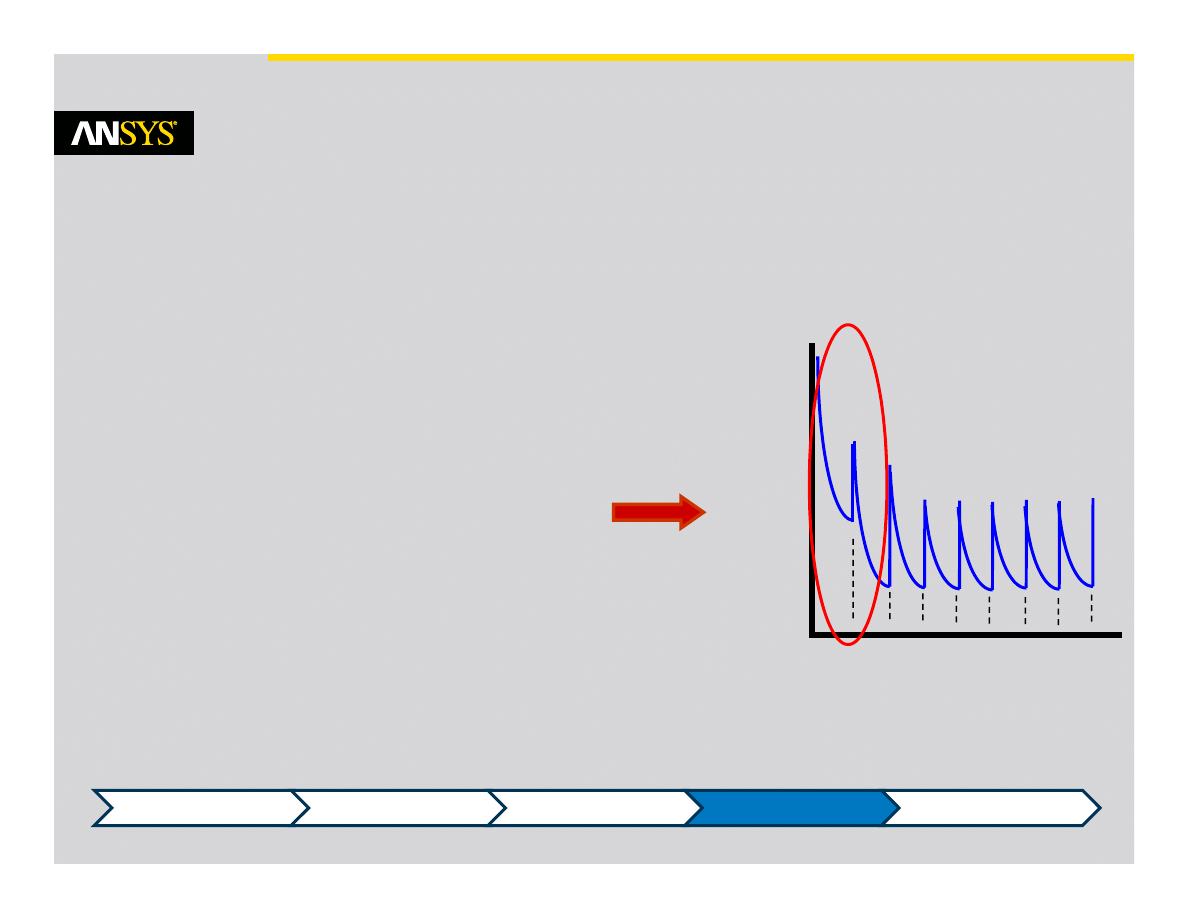
Initialization

•

Physically realistic initial conditions
should be used

–

A converged steady state solution is often
used as the starting point

•

If a transient simulation is started from
an approximate initial guess, the early
timesteps will not be accurate

–

The first few timesteps may not
converge

–

A smaller time step may be needed
initially to maintain solver stability

–

For cyclic behavior the first few cycles
can be ignored until a repeatable
pattern is obtained

4 6 8 10 12 14 16

Time (seconds)

Residuals

Introduction

Motivation

Setup

Time Steps

Output

January 16, 2012

Release 14.0

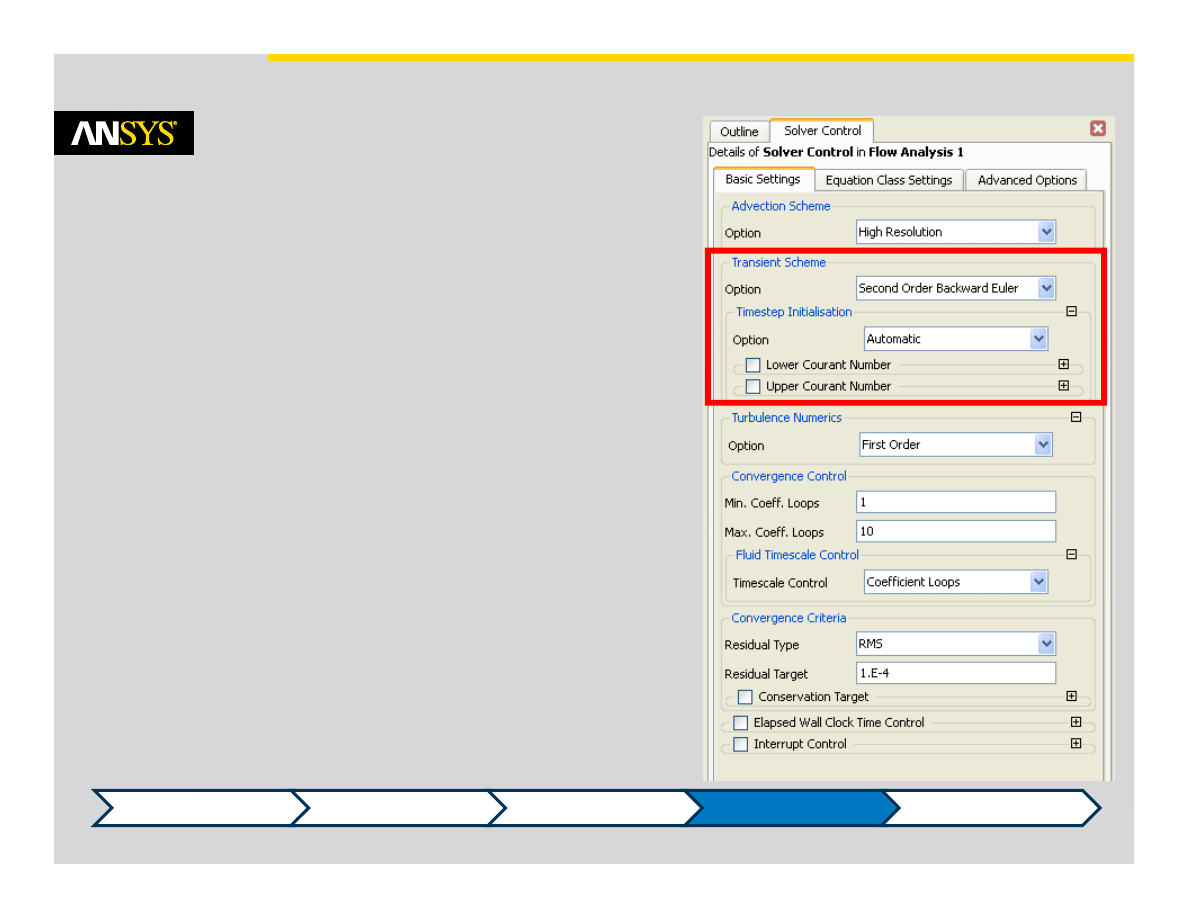
Solver Control

•

The transient scheme defines the numerical

algorithm for the transient term

•

Two implicit time‐stepping schemes are

available:

–

First Order Backward Euler (more stable)

–

Second Order Backward Euler (more accurate)

•

The default Second Order Backward Euler

scheme is generally recommended for most

transient runs

•

Timestep Initialisation controls the way the

previous timestep is used as the starting

point for the next timestep

–

Can use the last solution “as is”

–

Or the solver can extrapolate the previous

solution to try to provide a better starting point
• Not recommended at high Courant numbers

–

Automatic (default) switches between the two

depending on the Courant number

Introduction

Motivation

Setup

Time Steps

Output

January 16, 2012

Release 14.0

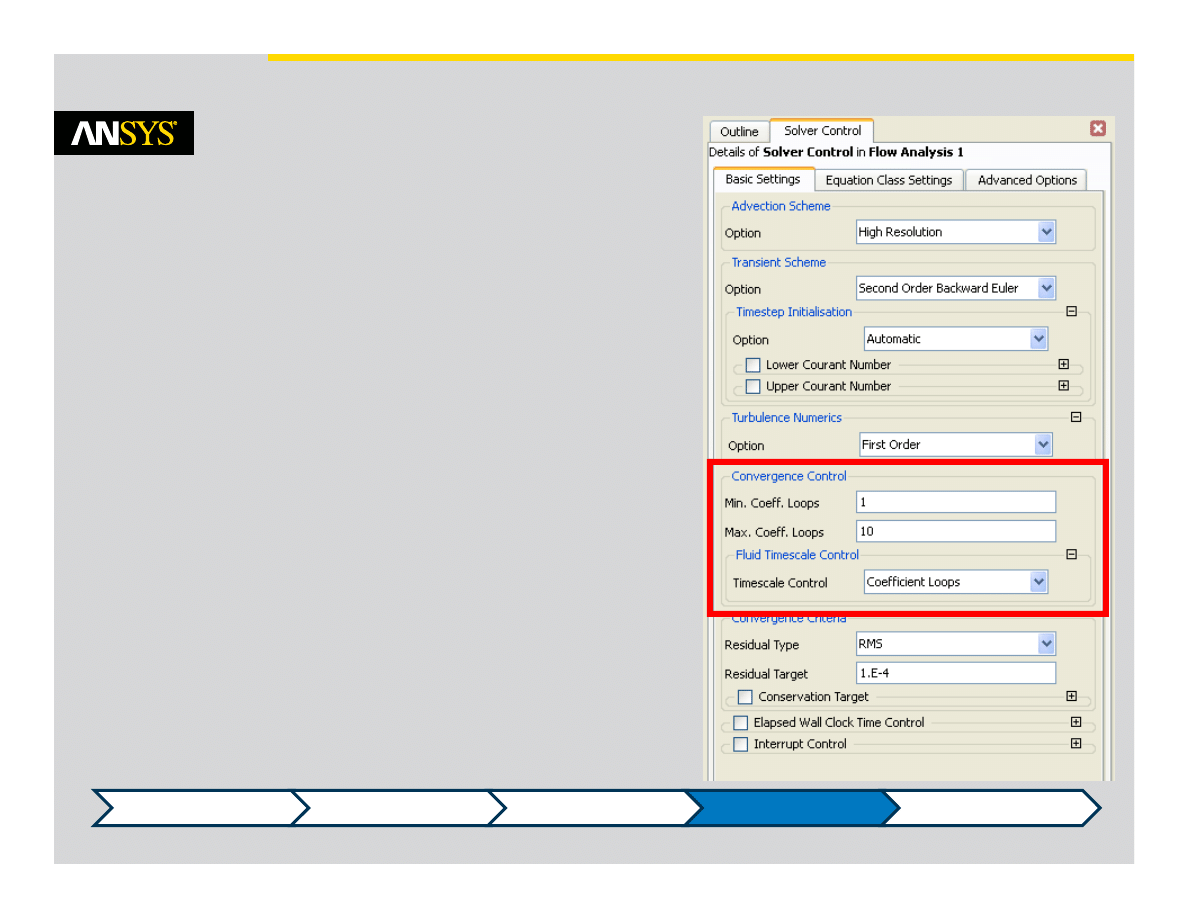
Solver Control

•

The Min. and Max. Coeff. Loops set limits on

the number of iteratins to use within each

timestep

•

Should aim to converge each timestep within

about 3‐5 loops

–

Complex physics may need more loops

•

If convergence is not achieved in the

maximum number of loops, it is generally

better to reduce the timestep size rather than

increase the number of loops

–

The solution will proceed to the next timestep
regardless of whether the convergence criteria
was met

–

Important to monitor the solution

Introduction

Motivation

Setup

Time Steps

Output

January 16, 2012

Release 14.0

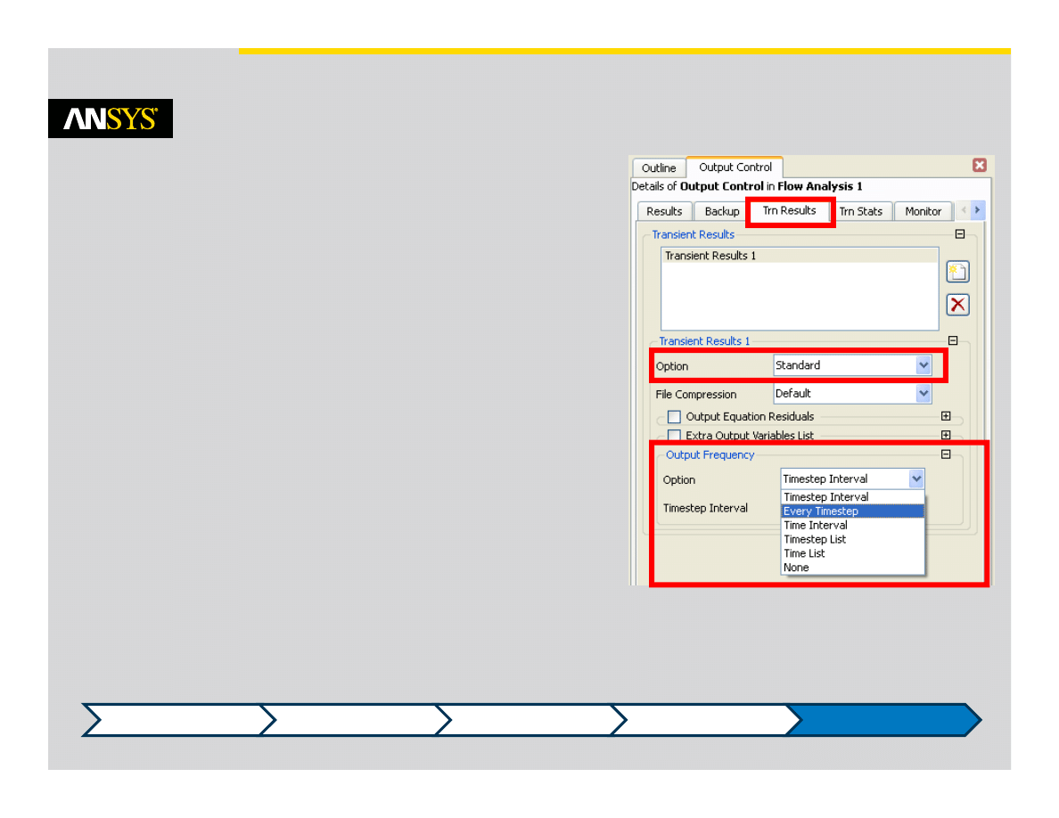
Output Control

•

Transient Results

–

By default only a final res file is written
• No information about the transient solution

–

Need to define the Transient Results under

Output Control

•

Transient Results Option

–

Standard
• Like a full results file
• Can take up a lot of disk space

–

Smallest
• Writes the smallest file which can still be used

for a restart (still quite large)

–

Selected Variables
• Pick only the variables of interest to give

smaller files

•

Output Frequency

–

Controls how often results are written

Introduction

Motivation

Setup

Time Steps

Output

January 16, 2012

Release 14.0

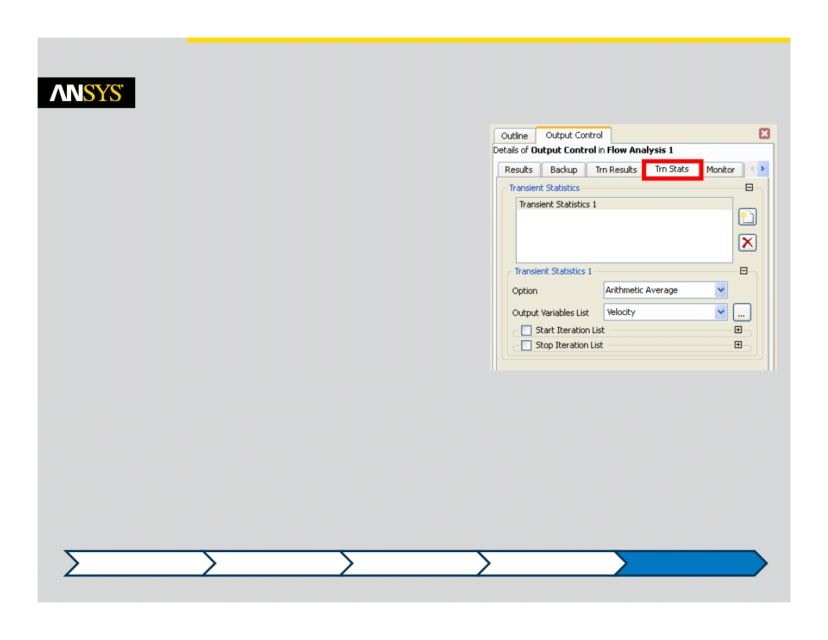
Output Control

•

Transient Statistics

–

Used to generate running statistics for solution

variables

•

Arithmetic Average, RMS, Minimum,

Maximum, Standard Deviation and Full

(everything) are available options

•

Pick the variables of interest

•

Start and Stop Iteration List defines when to

begin and end collecting the statistics

Introduction

Motivation

Setup

Time Steps

Output

January 16, 2012

Release 14.0

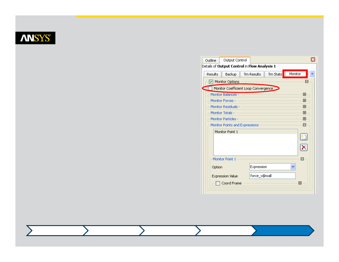
Output Control

•

Monitor Points are generally used as in

steady‐state simulations

•

Monitor Coefficient Loop Convergence

creates monitor history for each iteration

within a timestep

–

Useful to see if quantities of interest are

converging within a timestep

–

By default only the monitor values from the end

of the timestep are displayed

•

Tip: Monitoring an expression will create a

transient history chart in the Solver Manager.

This can be easier than creating the chart

from transient results files after‐the‐fact, and

it doesn’t require transient results files to be

written

Introduction

Motivation

Setup

Time Steps

Output

January 16, 2012

Release 14.0

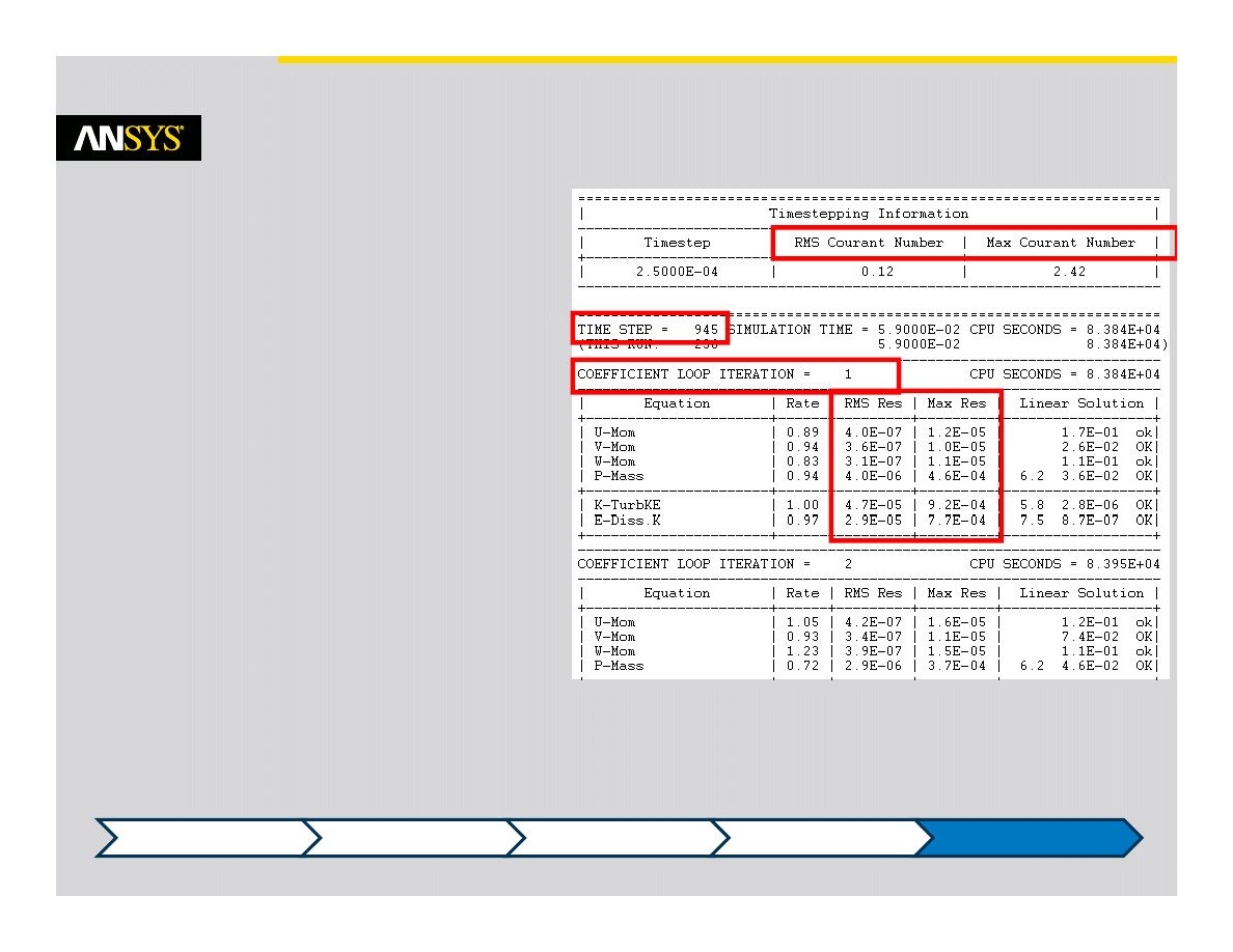
Solver Output

•

Output differs from steady

state in that each time step

now contains coefficient loop

output onitor Points are

generally used as in steady‐

state simulations

•

Courant number information

shown at the start of each

timestep

•

Make sure convergence has

been achieved by the end of

the timestep by monitoring the

RMS and MAX residual plots

Introduction

Motivation

Setup

Time Steps

Output

Wyszukiwarka

Podobne podstrony:

więcej podobnych podstron