A-58

Fourier Series

5. If in addition to the restrictions in (3) above, f (x) = f (L − x), then b

n

will be 0 for all even values of n. Thus in this case,

the expansion reduces to

∞

�

m=1

b

2m−1

sin

(2m − 1)πx

L

(The series in (4) and (5) are known as odd-harmonic series, since only the odd harmonics appear. Similar rules may be stated
for even-harmonic series, but when a series appears in the even-harmonic form, it means that 2L has not been taken as the
smallest period of f (x). Since any integral multiple of a period is also a period, series obtained in this way will also work,
but in general computation is simplified if 2L is taken to be the smallest period.)

6. If we write the Euler definitions for cos θ and sin θ, we obtain the complex form of the Fourier series known either as the

“Complex Fourier Series” or the “Exponential Fourier Series” of f (x). It is represented as

f (x) =

1
2

n=+∞

�

n=−∞

c

n

e

iω

n

x

where

c

n

=

1
L

�

L

−L

f (x) e

−iω

n

x

dx,

n = 0, ±1, ±2, ±3, . . .

with ω

n

=

nπ

L

for n = 0, ±1, ±2, . . . The set of coefficients c

n

is often referred to as the Fourier spectrum.

7. If both sine and cosine terms are present and if f (x) is of period 2L and expandable by a Fourier series, it can be represented

as

f (x) =

a

0

2 +

∞

�

n=1

c

n

sin

� nπx

L +

φ

n

�

,

where

a

n

= c

n

sin φ

n

,

b

n

= c

n

cos φ

n

,

c

n

=

�

a

2

n

+ b

2

n

,

φ

n

= arctan

� a

n

b

n

�

It can also be represented as

f (x) =

a

0

2 +

∞

�

n=1

c

n

cos

� nπx

L +

φ

n

�

,

where

a

n

= c

n

cos φ

n

,

b

n

= −c

n

sin φ

n

,

c

n

=

�

a

2

n

+ b

2

n

,

φ

n

= arctan

�

−

b

n

a

n

�

where φ

n

is chosen so as to make a

n

, b

n

, and c

n

hold.

8. The following table of trigonometric identities should be helpful for developing Fourier series.

n

n even

nodd

n/2 odd

n/2 even

sin nπ

0

0

0

0

0

cos nπ

(−1)

n

+1

−1

+1

+1

∗ sin

nπ

2

0

(−1)

(n−1)/2

0

0

∗ cos

nπ

2

(−1)

n/2

0

−1

+1

sin

nπ

4

√

2

2

(−1)

(n

2

+4n+11)/8

(−1)

(n−2)/4

0

*A useful formula for sin

nπ

2

and cos

nπ

2

is given by

sin

nπ

2 =

(i)

n+1

2

[(−1)

n

− 1] and cos

nπ

2 =

(i)

n

2

[(−1)

n

+ 1],

where i

2

= −1.

Auxiliary Formulas for Fourier Series

1 =

4

π

�

sin

π

x

k +

1
3

sin

3π x

k +

1
5

sin

5π x

k + · · ·

�

[0 < x < k]

x =

2k

π

�

sin

π

x

k −

1
2

sin

2π x

k +

1
3

sin

3π x

k − · · ·

�

[−k < x < k]

x =

k
2 −

4k

π

2

�

cos

π

x

k +

1

3

2

cos

3π x

k +

1

5

2

cos

5π x

k + · · ·

�

[0 < x < k]

x

2

=

2k

2

π

3

��

π

2

1 −

4
1

�

sin

π

x

k −

π

2

2

sin

2π x

k +

�

π

2

3 −

4

3

3

�

sin

3π x

k

−

π

2

4

sin

4π x

k +

�

π

2

5 −

4

5

3

�

sin

5π x

k + · · ·

�

[0 < x < k]

x

2

=

k

2

3 −

4k

2

π

2

�

cos

π

x

k −

1

2

2

cos

2π x

k +

1

3

2

cos

3π x

k −

1

4

2

cos

4π x

k + · · ·

�

[−k < x < k]

1 −

1
3 +

1
5 −

1
7 + · · · =

π

4

1 −

1

2

2

+

1

3

2

+

1

4

2

+ · · · =

π

2

6

1 −

1

2

2

+

1

3

2

−

1

4

2

+ · · · =

π

2

12

1 +

1

3

2

+

1

5

2

−

1

7

2

+ · · · =

π

2

8

1

2

2

+

1

4

2

+

1

6

2

+

1

8

2

+ · · · =

π

2

24

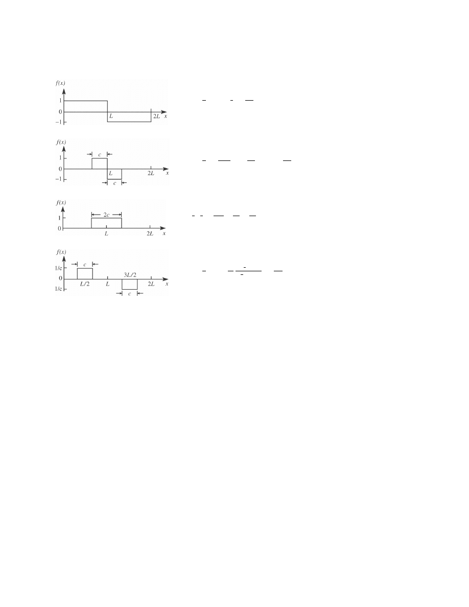
FOURIER EXPANSIONS FOR BASIC PERIODIC FUNCTIONS

f (x) =

4

π

�

n=1,3,5...

1

n

sin

nπ x

L

f (x) =

2

π

∞

�

n=1

(−1)

n

n

�

cos

nπc

L

− 1

�

sin

nπ x

L

f (x)=

c

L

+

2

π

∞

�

n=1

(−1)n

n

sin

nπc

L

cos

nπ x

L

f (x) =

2

L

∞

�

n=1

sin

nπ

2

sin(

1

2

nπc/L)

1

2

nπc/L

sin

nπ x

L

A-59

Auxiliary Formulas for Fourier Series

1 =

4

π

�

sin

π

x

k +

1
3

sin

3π x

k +

1
5

sin

5π x

k + · · ·

�

[0 < x < k]

x =

2k

π

�

sin

π

x

k −

1
2

sin

2π x

k +

1
3

sin

3π x

k − · · ·

�

[−k < x < k]

x =

k
2 −

4k

π

2

�

cos

π

x

k +

1

3

2

cos

3π x

k +

1

5

2

cos

5π x

k + · · ·

�

[0 < x < k]

x

2

=

2k

2

π

3

��

π

2

1 −

4
1

�

sin

π

x

k −

π

2

2

sin

2π x

k +

�

π

2

3 −

4

3

3

�

sin

3π x

k

−

π

2

4

sin

4π x

k +

�

π

2

5 −

4

5

3

�

sin

5π x

k + · · ·

�

[0 < x < k]

x

2

=

k

2

3 −

4k

2

π

2

�

cos

π

x

k −

1

2

2

cos

2π x

k +

1

3

2

cos

3π x

k −

1

4

2

cos

4π x

k + · · ·

�

[−k < x < k]

1 −

1
3 +

1
5 −

1
7 + · · · =

π

4

1 −

1

2

2

+

1

3

2

+

1

4

2

+ · · · =

π

2

6

1 −

1

2

2

+

1

3

2

−

1

4

2

+ · · · =

π

2

12

1 +

1

3

2

+

1

5

2

−

1

7

2

+ · · · =

π

2

8

1

2

2

+

1

4

2

+

1

6

2

+

1

8

2

+ · · · =

π

2

24

FOURIER EXPANSIONS FOR BASIC PERIODIC FUNCTIONS

f (x) =

4

π

�

n=1,3,5...

1

n

sin

nπ x

L

f (x) =

2

π

∞

�

n=1

(−1)

n

n

�

cos

nπc

L

− 1

�

sin

nπ x

L

f (x)=

c

L

+

2

π

∞

�

n=1

(−1)n

n

sin

nπc

L

cos

nπ x

L

f (x) =

2

L

∞

�

n=1

sin

nπ

2

sin(

1

2

nπc/L)

1

2

nπc/L

sin

nπ x

L

A-59

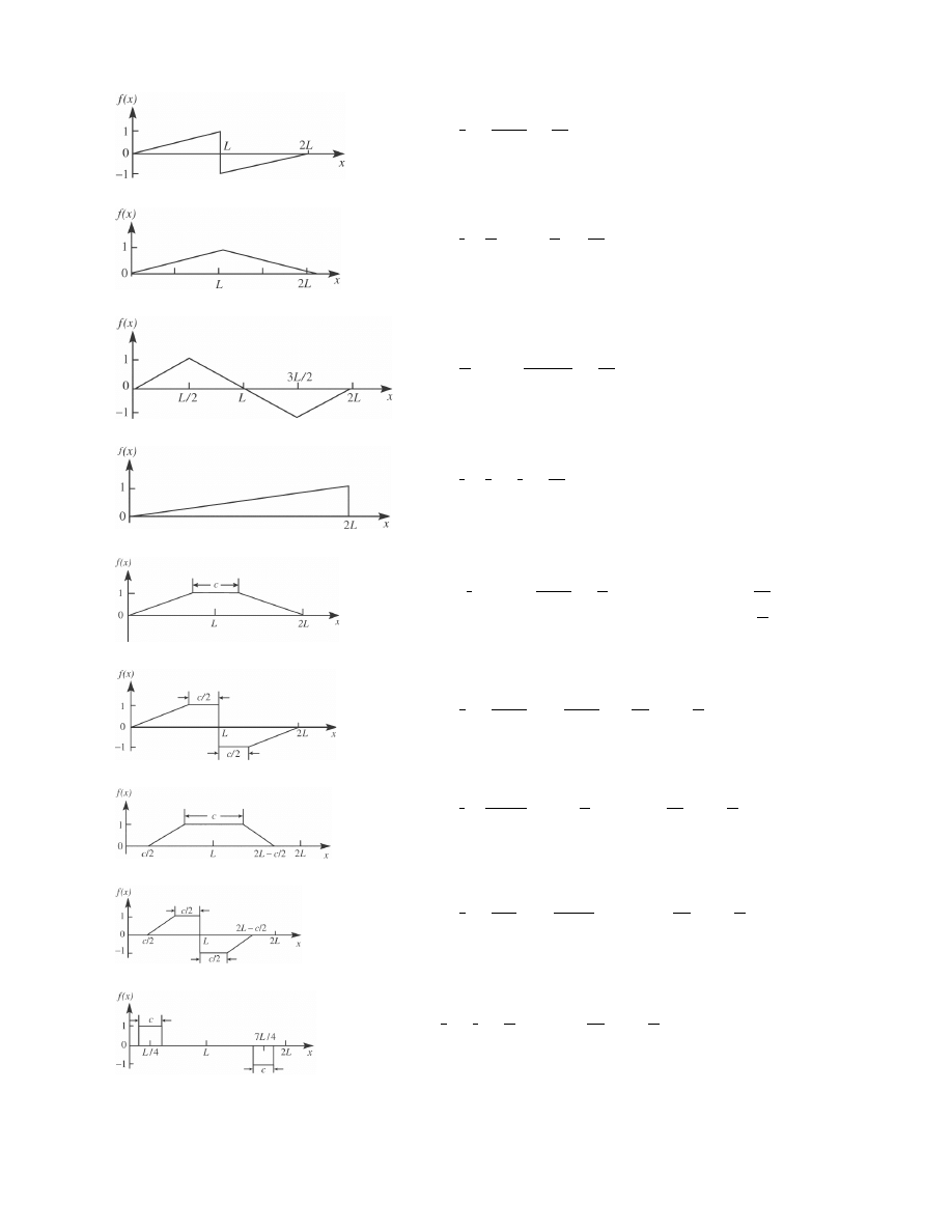
A-60

Fourier Expansions for Basic Periodic Functions

f (x) =

2

π

∞

�

n=1

(−1)

n+1

n

sin

nπ x

L

f (x) =

1

2

−

4

π

2

�

n=1,3,5,...

1

n

2

cos

nπ x

L

f (x) =

8

π

2

�

n=1,3,5,...

(−1)

(n−1)/2

n

2

sin

nπ x

L

f (x) =

1

2

−

1

π

∞

�

n=1

1

n

sin

nπ x

L

f (x) =

1

2

(1 + a) +

2

π

2

(1−a)

∞

�

n=1

1

n

2

[(−1)

n

cos nπa − 1] cos

nπ x

L

;

�

a =

c

2L

�

f (x) =

2

π

∞

�

n=1

(−1)

n−1

n

�

1 +

sin nπa

nπ(1−a)

�

sin

nπ x

L

;

�

a =

c

2L

�

f (x) =

1

2

−

4

π

2

(1−2a)

�

n=1,3,5,...

1

n

2

cos nπa cos

nπ x

L

;

�

a =

c

2L

�

f (x) =

2

π

∞

�

n=1

(−1)

n

n

�

1 +

1+(−1)

n

nπ(1−2a)

sin nπa

�

sin

nπ x

L

;

�

a =

c

2L

�

f (x)

4

π

∞

�

n=1

1

n

sin

nπ

4

sin nπa sin

nπ x

L

;

�

a =

c

2L

�

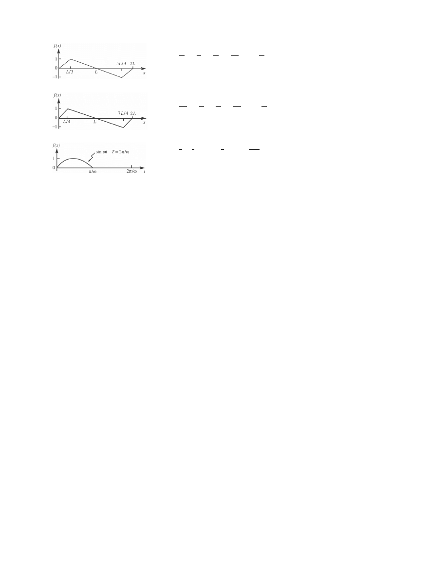
f (x) =

9

π

2

∞

�

n=1

1

n

2

sin

nπ

3

sin

nπ x

L

;

�

a =

c

2L

�

f (x) =

32

3π

2

∞

�

n=1

1

n

2

sin

nπ

4

sin

nπ x

L

;

�

a =

c

2L

�

f (x) =

1

π

+

1

2

sin ωt −

2

π

�

n=2,4,6,...

1

n

2

−1

cos nωt

Extracted from graphs and formulas, pages 372, 373, Differential Equations in Engineering Problems, Salvadori and Schwarz,
published by Prentice-Hall, Inc., 1954.

THE FOURIER TRANSFORMS

For a piecewise continuous function F (x) over a finite interval 0 ≤ x ≤ π; the finite Fourier cosine transform of F (x) is

f

c

(n) =

�

π

0

F (x) cos nx dx (n = 0, 1, 2, . . .)

If x ranges over the interval 0 ≤ x ≤ L, the substitution x

�

= π x/L allows the use of this definition, also. The inverse transform is

written.

F (x) =

1

π

f

c

(0) −

2

π

x

�

n=1

f

c

(n) cos nx (0 < x < π)

where F (x) =

F (x+�)+F (x−�)

2

. We observe that F (x+) = F (x−) = F (x) at points of continuity. The formula

f

(2)

c

(n) =

�

π

0

F

��

(x) cos nx dx

= −n

2

f

c

(n) − F

�

(0) + (−1)

n

F

�

(π)

(1)

makes the finite Fourier cosine transform useful in certain boundary value problems. Analogously, the finite Fourier sine transform
of F (x) is

f

s

(n) =

�

π

0

F (x) sin nx dx (n = 1, 2, 3, . . .)

and

F (x) =

2

π

∞

�

n=1

f

s

(n) sin nx (0 < x < π)

Corresponding to (1) we have

f

(2)

s

(n) =

�

π

0

F

��

(x) sin nx dx

(2)

= −n

2

f

s

(n) − n F (0) − n(−1)

n

F (π)

If F (x) is defined for x ≤ 0 and is piecewise continuous over any finite interval, and if

�

x

0

F (x) dx is absolutely convergent, then

f

c

(α) =

�

2

π

�

x

0

F (x) cos(αx) dx

A-61

A-60

Fourier Expansions for Basic Periodic Functions

f (x) =

2

π

∞

�

n=1

(−1)

n+1

n

sin

nπ x

L

f (x) =

1

2

−

4

π

2

�

n=1,3,5,...

1

n

2

cos

nπ x

L

f (x) =

8

π

2

�

n=1,3,5,...

(−1)

(n−1)/2

n

2

sin

nπ x

L

f (x) =

1

2

−

1

π

∞

�

n=1

1

n

sin

nπ x

L

f (x) =

1

2

(1 + a) +

2

π

2

(1−a)

∞

�

n=1

1

n

2

[(−1)

n

cos nπa − 1] cos

nπ x

L

;

�

a =

c

2L

�

f (x) =

2

π

∞

�

n=1

(−1)

n−1

n

�

1 +

sin nπa

nπ(1−a)

�

sin

nπ x

L

;

�

a =

c

2L

�

f (x) =

1

2

−

4

π

2

(1−2a)

�

n=1,3,5,...

1

n

2

cos nπa cos

nπ x

L

;

�

a =

c

2L

�

f (x) =

2

π

∞

�

n=1

(−1)

n

n

�

1 +

1+(−1)

n

nπ(1−2a)

sin nπa

�

sin

nπ x

L

;

�

a =

c

2L

�

f (x)

4

π

∞

�

n=1

1

n

sin

nπ

4

sin nπa sin

nπ x

L

;

�

a =

c

2L

�

f (x) =

9

π

2

∞

�

n=1

1

n

2

sin

nπ

3

sin

nπ x

L

;

�

a =

c

2L

�

f (x) =

32

3π

2

∞

�

n=1

1

n

2

sin

nπ

4

sin

nπ x

L

;

�

a =

c

2L

�

f (x) =

1

π

+

1

2

sin ωt −

2

π

�

n=2,4,6,...

1

n

2

−1

cos nωt

Extracted from graphs and formulas, pages 372, 373, Differential Equations in Engineering Problems, Salvadori and Schwarz,
published by Prentice-Hall, Inc., 1954.

THE FOURIER TRANSFORMS

For a piecewise continuous function F (x) over a finite interval 0 ≤ x ≤ π; the finite Fourier cosine transform of F (x) is

f

c

(n) =

�

π

0

F (x) cos nx dx (n = 0, 1, 2, . . .)

If x ranges over the interval 0 ≤ x ≤ L, the substitution x

�

= π x/L allows the use of this definition, also. The inverse transform is

written.

F (x) =

1

π

f

c

(0) −

2

π

x

�

n=1

f

c

(n) cos nx (0 < x < π)

where F (x) =

F (x+�)+F (x−�)

2

. We observe that F (x+) = F (x−) = F (x) at points of continuity. The formula

f

(2)

c

(n) =

�

π

0

F

��

(x) cos nx dx

= −n

2

f

c

(n) − F

�

(0) + (−1)

n

F

�

(π)

(1)

makes the finite Fourier cosine transform useful in certain boundary value problems. Analogously, the finite Fourier sine transform
of F (x) is

f

s

(n) =

�

π

0

F (x) sin nx dx (n = 1, 2, 3, . . .)

and

F (x) =

2

π

∞

�

n=1

f

s

(n) sin nx (0 < x < π)

Corresponding to (1) we have

f

(2)

s

(n) =

�

π

0

F

��

(x) sin nx dx

(2)

= −n

2

f

s

(n) − n F (0) − n(−1)

n

F (π)

If F (x) is defined for x ≤ 0 and is piecewise continuous over any finite interval, and if

�

x

0

F (x) dx is absolutely convergent, then

f

c

(α) =

�

2

π

�

x

0

F (x) cos(αx) dx

A-61