COSMOSM Advanced Modules
i
Contents
Introduction
. . . . . . . . . . . . . . . . . . . . . . . . . . . . . . . . . . 1-1
Design Optimization and Sensitivity . . . . . . . . . . . . . . . . . . . . . . . . . . . . . . .1-1
Terminology . . . . . . . . . . . . . . . . . . . . . . . . . . . . . . . . . . . . . . . . . . . . . . . . .1-2
Design Optimization Process . . . . . . . . . . . . . . . . . . . . . . . . . . . . . . . . . . . .1-3
Sensitivity Studies . . . . . . . . . . . . . . . . . . . . . . . . . . . . . . . . . . . . . . . . . . . . .1-3
Features of the Design Optimization and Sensitivity Module (OPTSTAR) .1-4
Elements of Optimization and Sensitivity
. . . . . . . . . . . . 2-1
Design Optimization . . . . . . . . . . . . . . . . . . . . . . . . . . . . . . . . . . . . . . . . . . .2-1
Design Variables . . . . . . . . . . . . . . . . . . . . . . . . . . . . . . . . . . . . . . . . . . . . . .2-2
Objective Function . . . . . . . . . . . . . . . . . . . . . . . . . . . . . . . . . . . . . . . . . . . .2-5
Behavior Constraints . . . . . . . . . . . . . . . . . . . . . . . . . . . . . . . . . . . . . . . . . . .2-5
Sensitivity Study . . . . . . . . . . . . . . . . . . . . . . . . . . . . . . . . . . . . . . . . . . . . . .2-6
Sensitivity Types . . . . . . . . . . . . . . . . . . . . . . . . . . . . . . . . . . . . . . . . . . . . . .2-8
Procedures and Examples
. . . . . . . . . . . . . . . . . . . . . . . 3-1
Introduction . . . . . . . . . . . . . . . . . . . . . . . . . . . . . . . . . . . . . . . . . . . . . . . . . .3-1
Overview of Process for Design Optimization and Sensitivity . . . . . . . . . . .3-2
Overview of Commands for Design Optimization and Sensitivity . . . . . . . .3-3
Procedures for Performing Design Optimization . . . . . . . . . . . . . . . . . . . . .3-5
Procedures for Performing Sensitivity Studies . . . . . . . . . . . . . . . . . . . . . .3-12
Special Features for Optimization and Sensitivity . . . . . . . . . . . . . . . . . . .3-14
In
de
x
In
de
x
Contents
ii
COSMOS/M Advanced Modules
Numerical Aspects
. . . . . . . . . . . . . . . . . . . . . . . . . . . . . 4-1
Introduction . . . . . . . . . . . . . . . . . . . . . . . . . . . . . . . . . . . . . . . . . . . . . . . . . .4-1
Basic Statements of Optimization Problems . . . . . . . . . . . . . . . . . . . . . . . . .4-2
Function Approximation . . . . . . . . . . . . . . . . . . . . . . . . . . . . . . . . . . . . . . . .4-2
Singular Value Decomposition . . . . . . . . . . . . . . . . . . . . . . . . . . . . . . . . . . .4-4
The Modified Feasible Direction Method . . . . . . . . . . . . . . . . . . . . . . . . . . .4-4
Overall Process . . . . . . . . . . . . . . . . . . . . . . . . . . . . . . . . . . . . . . . . . . . . .4-4
Search Direction . . . . . . . . . . . . . . . . . . . . . . . . . . . . . . . . . . . . . . . . . . . .4-5
Convergence to the Optimum . . . . . . . . . . . . . . . . . . . . . . . . . . . . . . . . . .4-6
Satisfaction of Kuhn-Tucker Conditions . . . . . . . . . . . . . . . . . . . . . . . . . .4-7
The Sequential Linear Programming Method . . . . . . . . . . . . . . . . . . . . . . . .4-9
Move Limits of Design Variables . . . . . . . . . . . . . . . . . . . . . . . . . . . . . . . .4-10
Constraint Trimming . . . . . . . . . . . . . . . . . . . . . . . . . . . . . . . . . . . . . . . . . .4-11
Convergence Criteria . . . . . . . . . . . . . . . . . . . . . . . . . . . . . . . . . . . . . . . . . .4-12
References . . . . . . . . . . . . . . . . . . . . . . . . . . . . . . . . . . . . . . . . . . . . . . . . . .4-14
Additional Problems
. . . . . . . . . . . . . . . . . . . . . . . . . . . . 5-1
Index . . . . . . . . . . . . . . . . . . . . . . . . . . . . . . . . . . . . . . . . . . . 1-1
In
de
x
In
de
x

COSMOSM Advanced Modules
1-1
1
Introduction
Design Optimization and Sensitivity
Before starting the topic of design optimization and sensitivity, it is important to
distinguish between analysis and design. Analysis is the process of determining the
response of a specified system to its environment. Design, on the other hand, is the
actual process of defining the system. Analysis is therefore a subset of design.
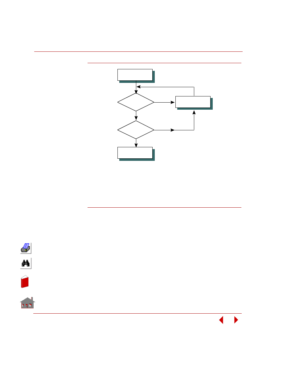
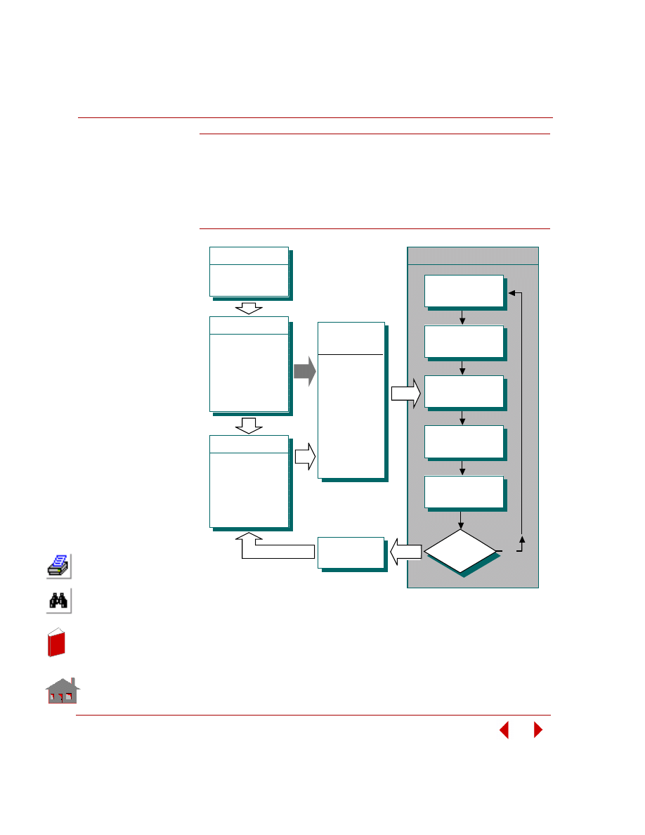
Engineering design in general, is an iterative process as shown in Figure 1-1. The
design is continuously modified until it meets evaluation and acceptance criteria set
by the engineer. Mathematical and empirical formulas aided by years of
engineering judgment and experience have been useful in the traditional design
processes to verify the adequacy of designs. However, a fully automated design
optimization and sensitivity is used when engineers are trying to modify a design
which level of complexity exceeds their ability to make appropriate changes. It is
not surprising that even what might appear as extremely simple design task may
easily be a real challenge to the designer during the decision-making process.
The design optimization and sensitivity capability provides many design options.
Whether you wish to design a simple truss or a complicated three dimensional solid
model, COSMOSM or COSMOSFFE will modify both the size and geometrical
shape in search for an improved design.
In
de
x
In
de
x
Chapter 1 Introduction
1-2
COSMOSM Advanced Modules
Figure 1-1. Iterative Process of Engineering Design
The following sections provide more information on the design optimization and
sensitivity module (OPTSTAR). They include brief explanations of terminology,
the optimization process, and sensitivity studies. There is also a summary of the
important features of the OPTSTAR module.
Terminology
The terminology frequently used in design optimization and sensitivity study are:
design variables, objective function, behavior constraints, response quantities,
feasible design, optimum design, and sensitivity type. Chapter 2, Elements of
Design Optimization and Sensitivity, explains these terminology in more detail.
Initial Design
Requirements
Satisfied
?
Any
Room for
Improvments
?
Final Design
Yes
Yes
No
Change Design
No
In
de
x
In
de
x
COSMOSM Advanced Modules
1-3
Part 2 OPSTAR / Optimization
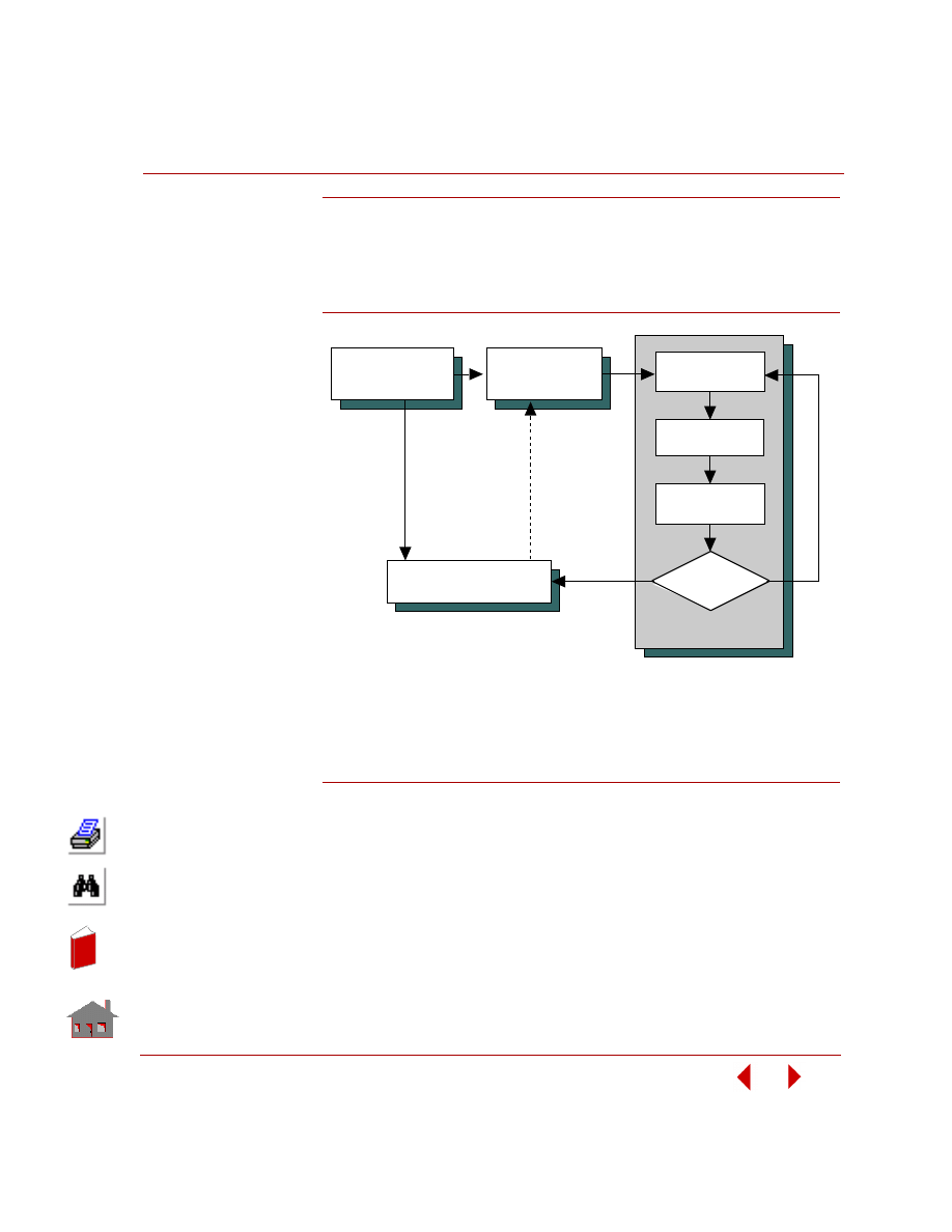
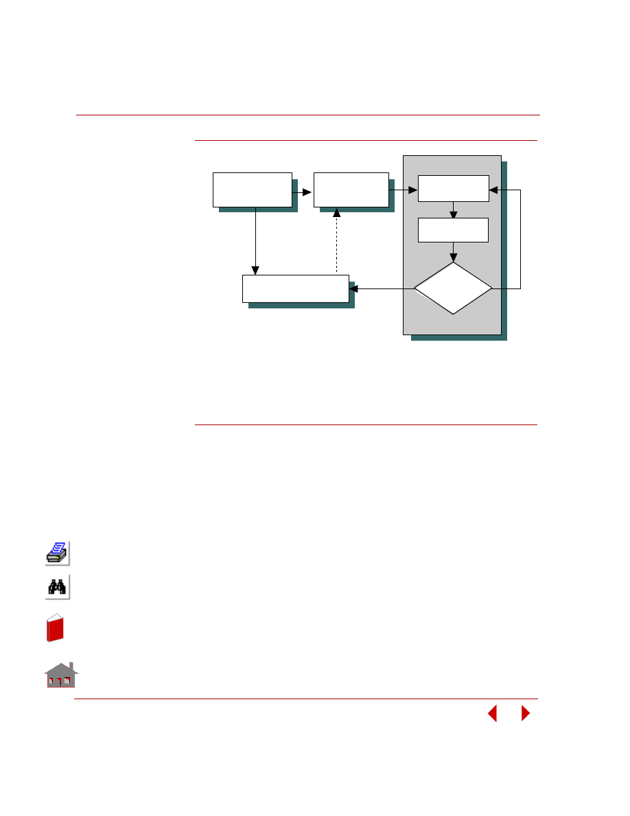
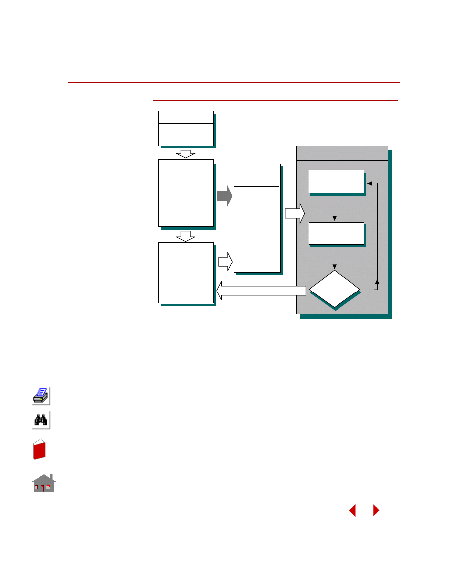
Design Optimization Process
The process of design optimization can be pictorially represented as shown in the
following figure.
Figure 1-2. Design Optimization Process
Refer to Chapter 3, Procedures and Examples, for general guidelines to performing
design optimization.
Sensitivity Studies
The process of sensitivity study is similar in principle to the design optimization
process illustrated previously. The procedure is summarized in Figure 1-3.
POSTPROCESSING
GEOMETRY
MESHING
APPROXIMATION
AND OPTIMIZATION
O P TIMIZATIO N LO O P
GEOMETRY, MESHING,
AND ANALYSIS
DEFINE
OPTIMIZATION
PARAMETERS
ANALYSIS
Yes
Is
Convergence
Achieved
?
No
In
de
x
In
de
x
Chapter 1 Introduction
1-4
COSMOSM Advanced Modules
Figure 1-3. Sensitivity Process
Chapter 3, Procedures and Examples, describes more details about performing
sensitivity studies.
Features of the Design Optimization and
Sensitivity Module (OPTSTAR)
The process of finite element analysis, evaluation of analysis results and design
changes, and modifications for yet another solution phase are performed
automatically in COSMOSM. OPTSTAR performs two-dimensional and three-
dimensional sizing and shape optimization and sensitivity for structural and thermal
applications. The following are some of the module's capabilities:
•
Full interaction with GEOSTAR for model creation, results manipulation and
display (pre- and postprocessing)
•
Access to COSMOSM and COSMOSFFE solvers, element and material
libraries
POSTPROCESSING
GEOMETRY
MESHING
No
S E NS ITIV ITY LO O P
Yes
Is
Required
Number of Runs
Executed
?
GEOMETRY, MESHING,
AND ANALYSIS
DEFINE
SENSITIVITY
PARAMETERS
ANALYSIS
In
de
x
In
de
x

COSMOSM Advanced Modules
1-5
Part 2 OPSTAR / Optimization
•
Type of analyses:
– Linear Static (including multiple load cases)
– Linear Dynamic (natural frequencies and mode shapes)
– Linearized Buckling
– Heat Transfer
– Nonlinear
– Fatigue
– Advanced Dynamic
– Dynamic Stress
•
Design variables:
– Side constraints (upper and lower limits of design variables)
– Move limits control
– Shape Applications
- Dimensions and parameters used in building the model's geometry
–Sizing Applications
- Parameters used to define the model other than the shape parameters
- For linear static analysis, predefined sizing options include:
•
Cross-sectional area of truss elements
•
Thickness of 2D continuum elements
•
Thickness of shell elements
•
Width and height of beam elements with rectangular cross-sections
•
Thickness and radius of pipe elements
•
Optimization behavior constraints:
– Trimming control
– Different sets (with lower and upper limits) of:
- Displacements
- Relative displacements
- Stresses
- Strains
- Reaction forces
- Fatigue usage factors
In
de
x
In
de
x

Chapter 1 Introduction
1-6
COSMOSM Advanced Modules
- Natural frequencies
- Linearized buckling load factors
- Velocities
- Accelerations
- Temperatures
- Temperature gradients
- Heat Fluxes
- Weight
- Volume
- User-defined quantities
•
Optimization objective function:
– Minimization and maximization of one type composed of different sets with
user-specified weight factors.
- Volume
- Weight
- Displacement
- Relative displacement
- Stress
- Strain
- Reaction force
- Fatigue usage factors
- Velocity
- Acceleration
- Natural frequency
- Linearized buckling load factor
- Temperature
- Temperature gradient
- Heat flux
- User-defined quantity
In
de
x
In
de
x

COSMOSM Advanced Modules
1-7
Part 2 OPSTAR / Optimization
•
Sensitivity options:
– Global, local and offset pre-optimization sensitivity studies, in addition to
optimization sensitivity results.
– Sensitivity response quantities include:
- Displacements
- Relative displacements
- Stresses
- Strains
- Reaction forces
- Fatigue usage factors
- Velocities
- Accelerations
- Natural frequencies
- Linearized buckling load factors
- Temperatures
- Temperature gradients
- Heat fluxes
- Volume
- Weight
- User-defined quantities
•
Numerical techniques:
– Modified Feasible Directions
– Singular Value Decomposition technique
– Linear, quadratic and cubic approximations
– Restart and restore options
•
Results:
– Output file
– X-Y convergence and sensitivity plots
– Color filled, colored line contour plots, and vector plots of displacement,
stress, strain, temperature, temperature gradient, and heat flux for the current
model.
In
de
x
In
de
x

Chapter 1 Introduction
1-8
COSMOSM Advanced Modules
– Animation and plots of deformed shapes for linear static analysis and mode
shapes for frequency and buckling analyses.
–Tabular data reports
Limits
•
25 design variables
•
60 constraint sets
•
100 objective function sets
•
60 sensitivity response quantities
•
75 design sets for optimization
•
20 increments for global sensitivity
•
20 sets for offset sensitivity
•
32,000 and 64,000 nodes and elements on PCs
•
3000 nodes and 3000 elements for EXPLORER
•
64,000 nodes and 64,000 elements on EWS (Unix workstations)
In
de
x
In
de
x
COSMOSM Advanced Modules
2-1
2
Elements of Optimization
and Sensitivity
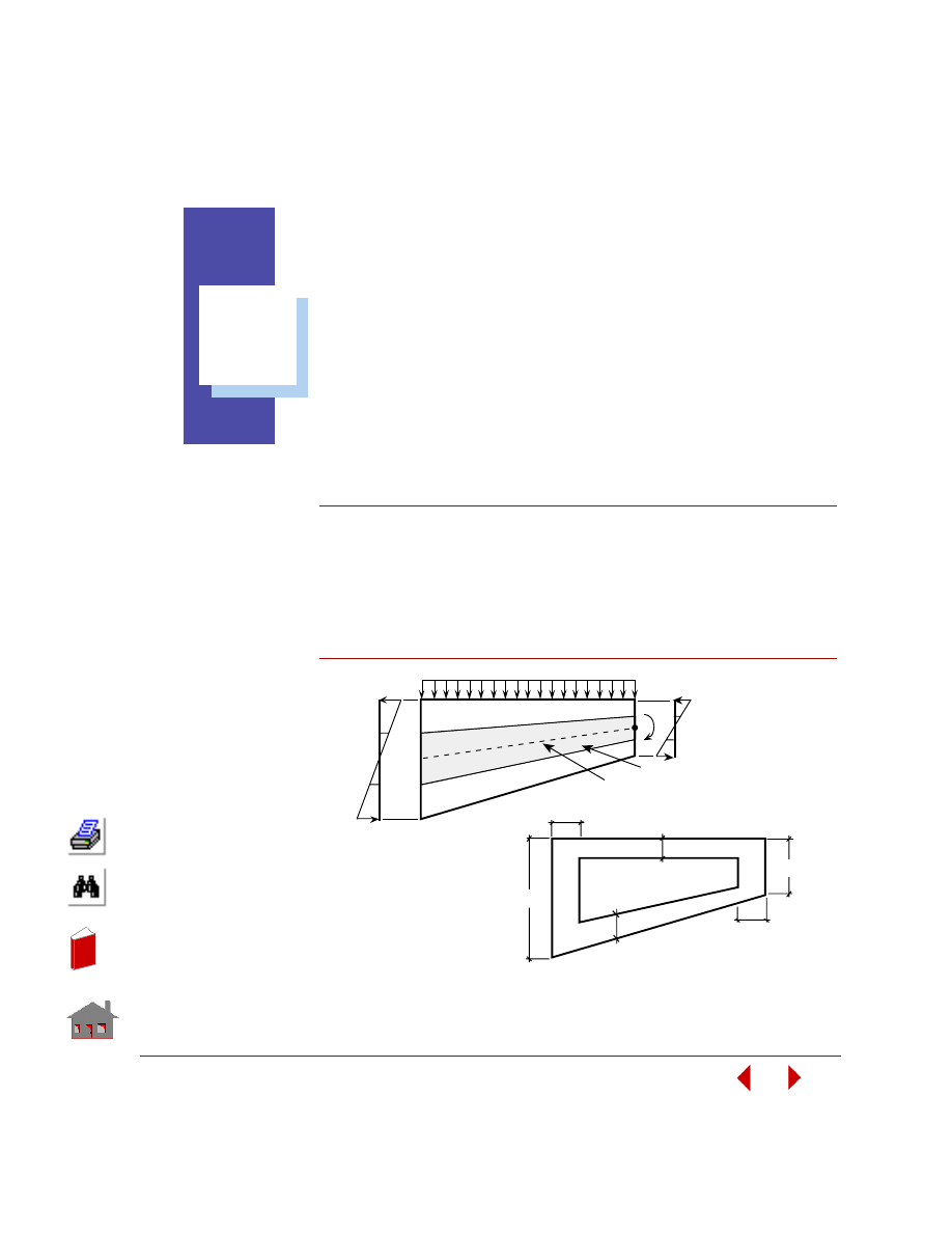
Design Optimization
Design optimization refers to the automated redesign process that attempts to
minimize or maximize a specific quantity (objective function) subject to limits or
constraints on the response by using a rational mathematical approach to yield
improved designs. Figure 2-1 shows minimum weight design of a structure.
Figure 2-1. Minimum Weight Design of a Structure
t
Fina l D e sign
Remov able Material
Neutral Axis
Initia l D e sign
3
d
2
1
t
1
t
2
t
4
d
In
de
x
In
de
x
Chapter 2 Elements of Optimization and Sensitivity
2-2
COSMOSM Advanced Modules
A feasible design is a design that satisfies all of the constraints. A feasible design
may not be optimal. An optimum design is defined as a point in the design space for
which the objective function is minimized or maximized and the design is feasible.
If relative minima exist in the design space, other optimal designs can exist.
Basic terminology in design optimization are: Design variables, objective function,
and behavior constraints. They are explained in the following sections.
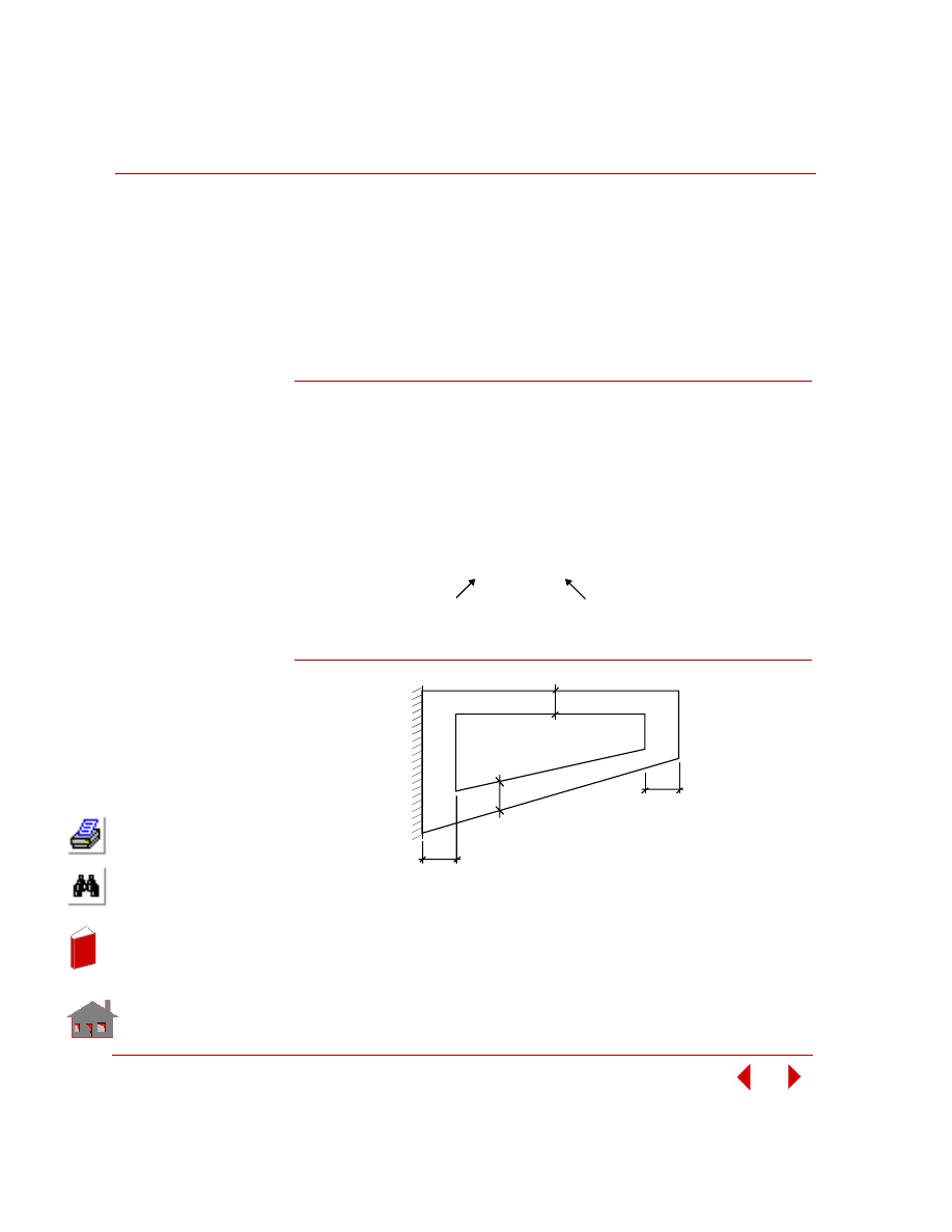
Design Variables
Design variables are the parameters (independent quantities) that users seek to find
their values for an optimum design. Figure 2-2 shows a structure having four
geometry dimensions defined as design variables.
Upper and lower bounds are specified for each design variable. Lower and upper
bounds are also referred to as side constraints.
For example:
Figure 2-2. A Structure with Four Design Variables
10
≤ T1 ≤ 25
Lower Bound
Upper Bound
t
t
1
t
2
t
4
3
In
de
x
In
de
x
COSMOSM Advanced Modules
2-3
Part 2 OPSTAR / Optimization
Depending on design variables, there are two types of optimization applications:
sizing optimization and shape optimization.
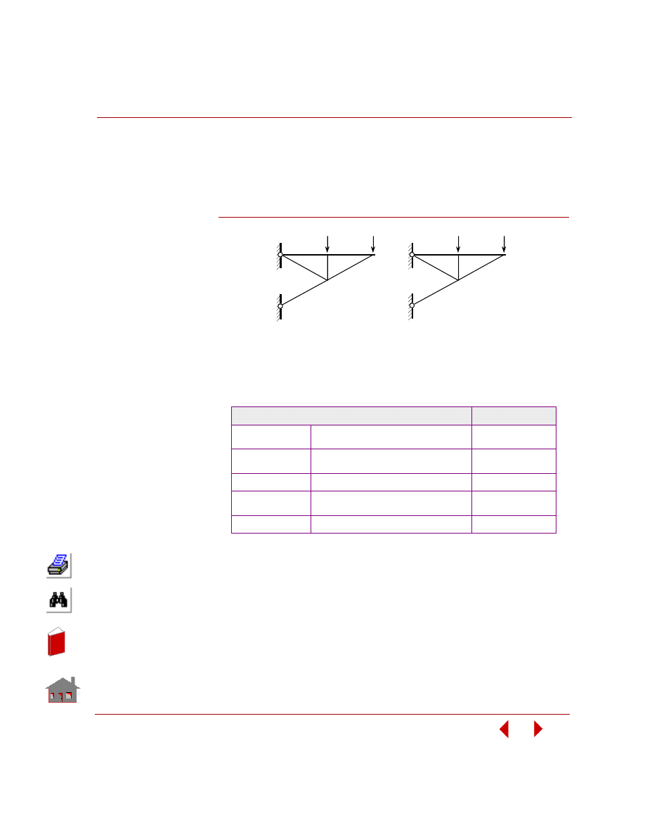
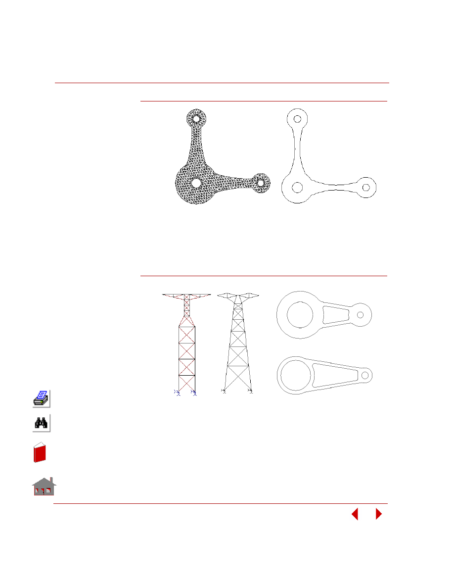
Sizing optimization refers to the class of problems where a change in design
variables does not change the problem's geometry or mesh as shown in Figure 2-3.
Figure 2-3. Initial and Final Geometry and Mesh for a Sizing Optimization Problem
For linear static analysis, predefined sizing options are summarized in Table 2-1.
Table 2-1. Predefined Sizing Options
Shape optimization refers to the class of problems where any change in design
variables causes change in the problem's geometry or mesh as shown in Figure 2-4.
COSMOSM Element Type and Name
Design Variable
Truss TRUSS2D,
TRUSS3D
Cross-Sectional
Area
Beam
(rectangular
cross-sections)
BEAM2D, BEAM3D
Width, Height
2D Continuum
TRIANG, PLANE2D
Thickness
Shell
SHELLAX, SHELL3, SHELL3T, SHELL4,
SHELL4T, SHELL6, SHELL9
Thickness
Pipe PIPE
Thickness,
Radius
Final Ge ome try and Me sh
Initial Ge ome try and Me sh
=
In
de
x
In
de
x
Chapter 2 Elements of Optimization and Sensitivity
2-4
COSMOSM Advanced Modules
Figure 2-4. Initial and Final Geometry and Mesh for a Shape Optimization Problem
Besides purely sizing optimization and shape optimization mentioned above, there
is a class of problems where both sizing and shape parameters are defined as design
variables as shown in Figure 2-5.
Figure 2-5. Initial and Final Geometry for Sizing/Shape Optimization Problems
Final Geometry
Initial Geometry and Mesh
Initial Geometry
Sizing Parameter: Thickness
Sizing Parameter: Cross-Section Area
Final Geometry
Initial Geometry
Final Geometry
Truss Elements
Shell Elements
or Continuum Elements
In
de
x
In
de
x
COSMOSM Advanced Modules
2-5
Part 2 OPSTAR / Optimization
Objective Function
Objective function is a single quantity that the optimizer seeks to minimize or
maximize. The objective function must be a continuous function of the design
variables. The weight (or volume) of a structure is an example of the commonly
used objective functions. Other quantities are:
•
Stress,
•
Strain,
•
Displacement,
•
Reaction Force,
•
Velocity,
•
Acceleration,
•
Natural Frequency,
•
Linearized Buckling
Load Factor,
•
Temperature,
•
Temperature Gradient,
•
Heat Flux,
•
Fatigue Usage Factor,
and
•
User-Defined Functions.
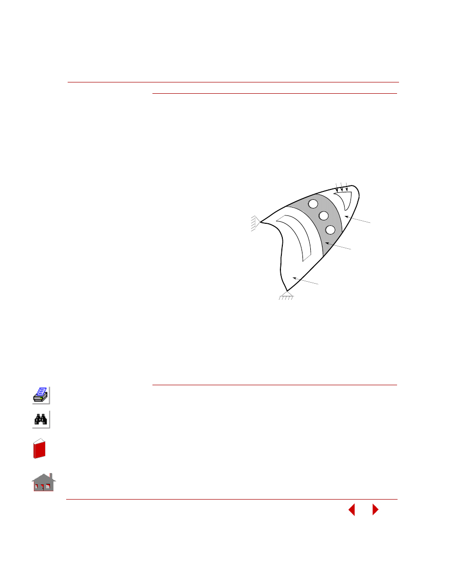
The objective function can be composed of different sets of the same type, and can
reflect different weight (importance) factors for different portions of the model as
shown in Figure 2-6.
Behavior Constraints
A behavior constraint is defined as an inequality that must be satisfied in order to
have a feasible design. The behavior constraints are typically response quantities
that are functions of the design variables. Von Mises stress is a typical example in
structural problems:
von Mises stress
≤ allowed stress
Rg
3
Rg
2
Rg
1
Figure 2-6. A Structure Composed of Three Regions
In
de
x
In
de
x
Chapter 2 Elements of Optimization and Sensitivity
2-6
COSMOSM Advanced Modules
Other quantities are:
•
Volume,
•
Weight,
•
Stress,
•
Strain,
•
Displacement,
•
Reaction Force,
•
Velocity,
•
Acceleration,
•
Natural Frequency,
•
Linearized Buckling Load Factor,
•
Temperature,
•
Temperature Gradient,
•
Heat Flux,
•
Fatigue Usage Factor, and
•
User-Defined Functions.
Multiple constraint sets of different types can also be specified.
In COSMOSM, users have to specify lower and upper limits for behavior
constraints.
For example:
0
≤ von Mises stress ≤ allowed stress
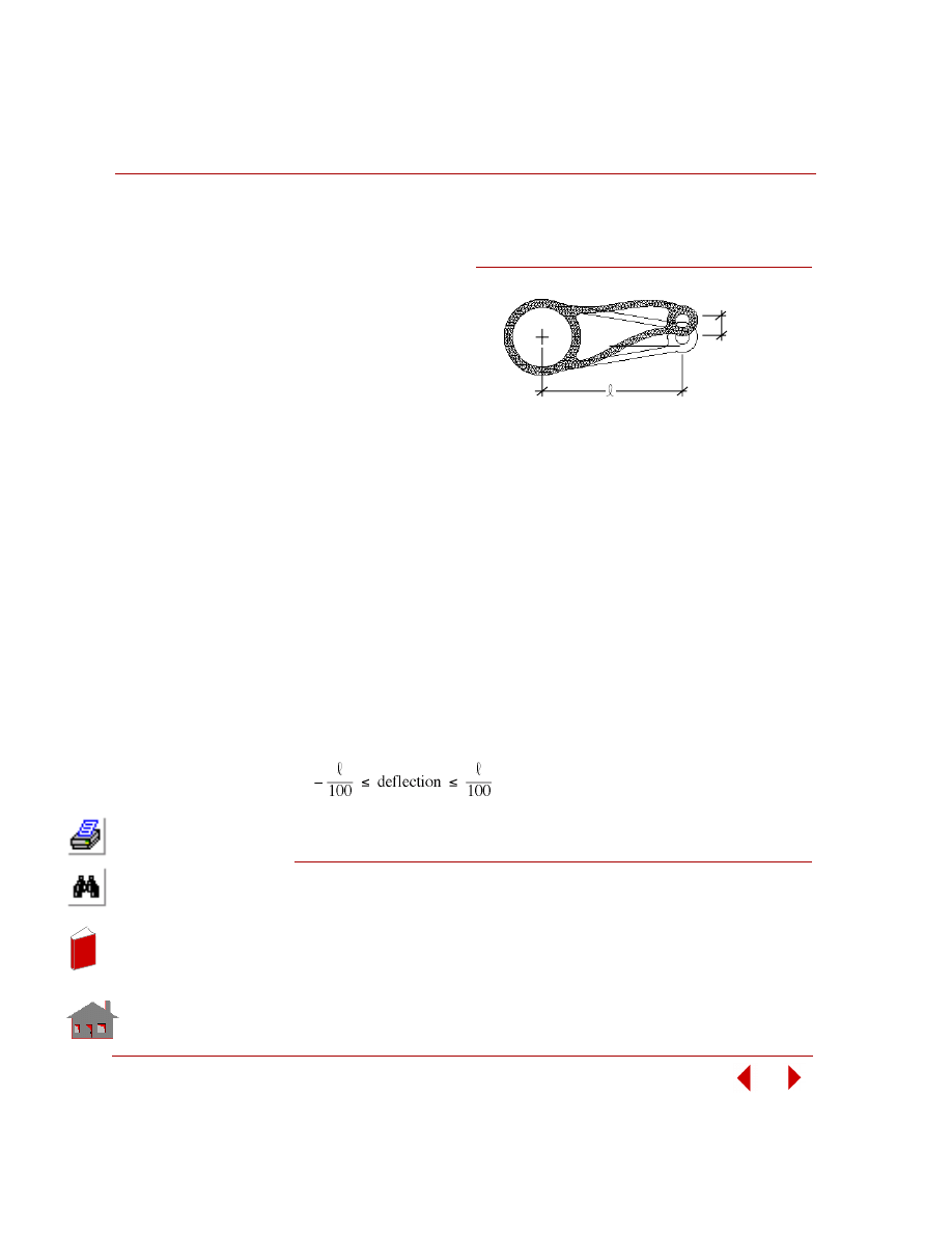
Sensitivity Study
A sensitivity study is the procedure that determines the changes in a response
quantity for a change in a design variable. Figure 2-8 shows a sensitivity study of a
control arm bracket and Figure 2-9 shows its result.
Figure 2-7. An Optimization Problem with Stress
and Displacement Constraint
Deflection
In
de
x
In
de
x
COSMOSM Advanced Modules
2-7
Part 2 OPSTAR / Optimization
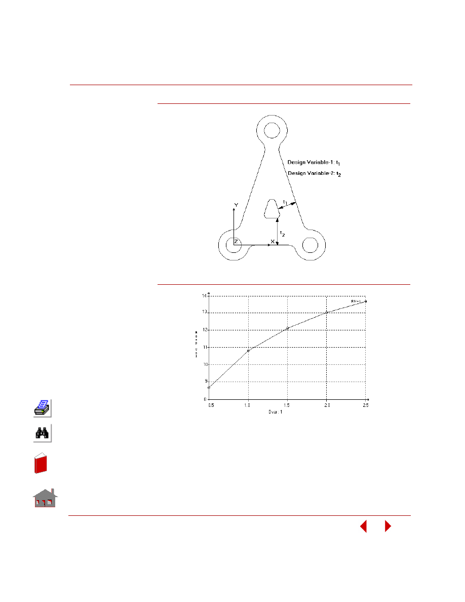
Figure 2-8. Sensitivity Study of a Control Arm Bracket in Frequency Analysis
Figure 2-9. Fundamental Frequency versus Design Variable-1, t
1
Basic terminology in sensitivity study are: Design variables and response
quantities. The definition of design variables is the same as that in design
optimization. Response quantities are functions of the design variables. All the
postprocessing quantities which are suitable for the objective function and behavior
constraints are also suitable for the sensitivity response quantities.
In
de
x
In
de
x
Chapter 2 Elements of Optimization and Sensitivity
2-8
COSMOSM Advanced Modules
Sensitivity Types
There are four types of sensitivity study, namely, global sensitivity, offset
sensitivity, local sensitivity, and optimization sensitivity results. They are explained
in the following paragraphs.
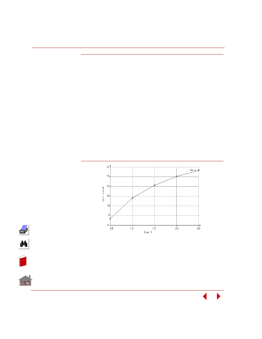
Global sensitivity - where design variables are changed between their lower and
upper bounds in a user-specified number of steps. The number of steps is the same
for all the design variables. Under this type of sensitivity, the user can change all the
design variables simultaneously or one at a time.
Have the frequency analysis of a control arm bracket as an example where:
0.5
≤ design variable-1 ≤ 2.5 and
1.5
≤ design variable-2 ≤ 3.5
The plots of response quantity versus design variable are shown in Figure 2-10
through Figure 2-12.
Figure 2-10. Global Sensitivity - One at a Time: Fundamental Frequency
versus Design Variable-1, t
1
In
de
x
In
de
x
COSMOSM Advanced Modules
2-9
Part 2 OPSTAR / Optimization
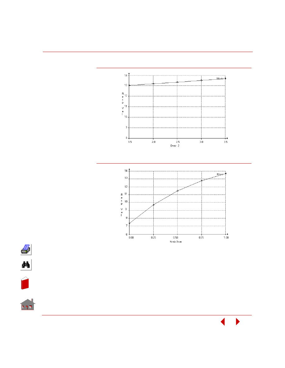
Figure 2-11. Global Sensitivity - One at a Time: Fundamental Frequency
versus Design Variable-2, t
2
Figure 2-12. Global Sensitivity - Simultaneously: Fundamental Frequency
versus Normalized Design Variable-1and -2
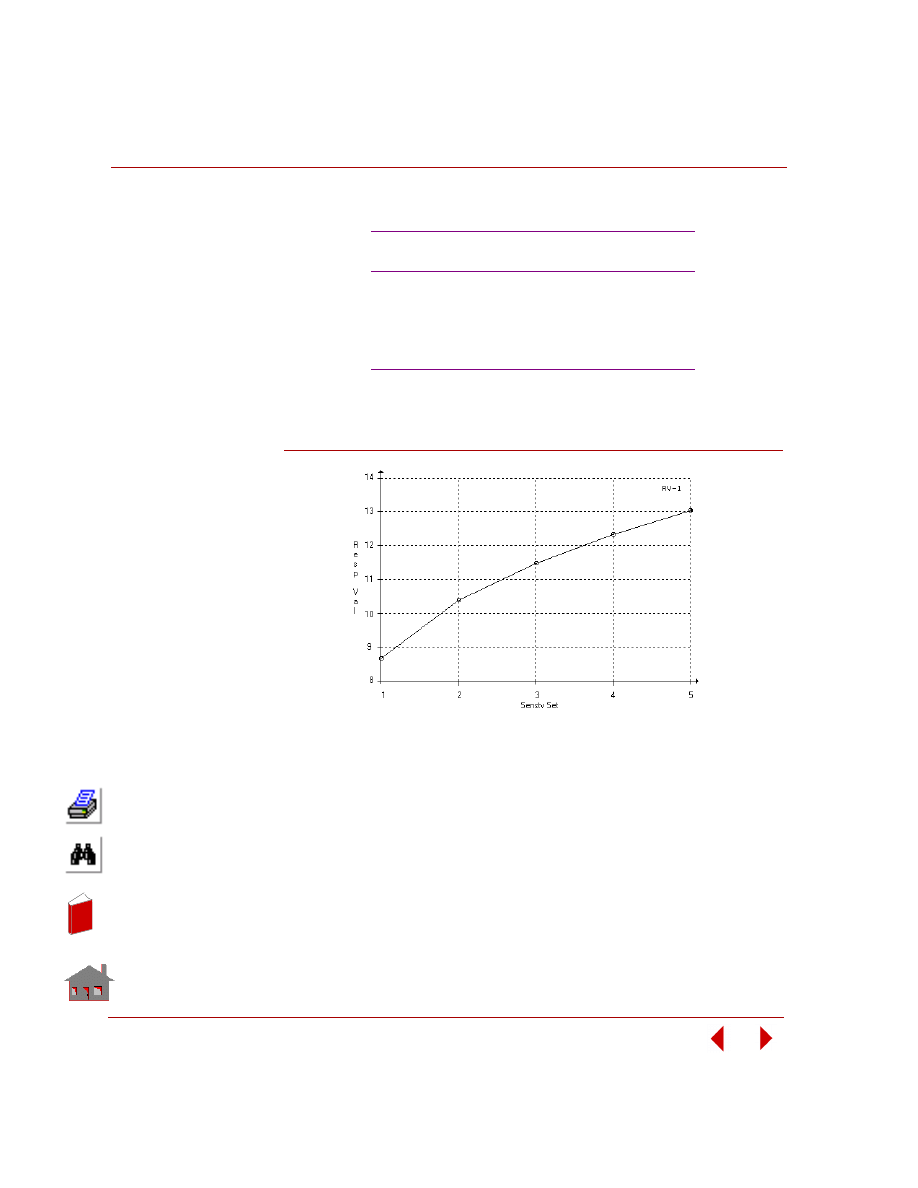
Offset sensitivity - where users specify the values of a series of design variables in
a user-defined sets. The design variables are defined either by the actual values or
by a perturbation ratio with respect to the initial value.
In
de
x
In
de
x
Chapter 2 Elements of Optimization and Sensitivity
2-10
COSMOSM Advanced Modules
Have the frequency analysis of a control arm bracket as an example where the
series of design variables are:
The plot of response quantity versus sensitivity set is shown in Figure 2-13.
Figure 2-13. Offset Sensitivity: Fundamental Frequency versus
Sensitivity Set Number
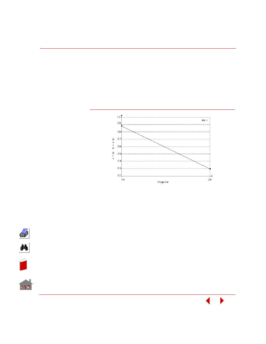
Local sensitivity - where a design variable is perturbed at a time by a user-
specified value while the rest of the design variables are kept unchanged. The
perturbed design variables are defined either by the actual values or by a
perturbation ratio with respect to the initial value. The gradients of the response
quantities with respect to the design variables are computed based on the finite
difference method.
Have the frequency analysis of a control arm bracket as an example where:
Sensitivity Set
Number
Design
Variable-1
Design
Variable-2
1
0.5
3.5
2
1.0
3.0
3
1.5
2.5
4
2.0
2.0
5
2.5
1.5
In
de
x
In
de
x
COSMOSM Advanced Modules
2-11
Part 2 OPSTAR / Optimization
The plot of gradient of the response quantity versus design variable set is shown in
Figure 2-14.
Figure 2-14. Local Sensitivity: Gradient of Fundamental Frequency
versus Design Variable Number
Optimization sensitivity results - where gradients of behavior constraints and
objective function are computed during the optimization process. The gradients are
obtained by taking the derivatives of the approximation functions with respect to
the design variables. This type of sensitivity study is available only when the design
optimization is to be performed.
Initial Value:
design variable-1=2.5,
design variable-2=3.5
Perturbation Ratio:
design variable-1=+0.1,
design variable-2=+0.1
In
de
x
In
de
x

2-12
COSMOSM Advanced Modules
In
de
x
In
de
x
COSMOSM Advanced Modules
3-1
3
Procedures and Examples
Introduction
This chapter presents detailed examples that fully describes the procedures for
performing design optimization and sensitivity in COSMOSM. The descriptions
include: selection and definition of appropriate parameters required for geometry
creation, generation of the finite element mesh parametrically or otherwise,
applying loads and boundary conditions, optimization constraint definitions,
defining the objective function, defining sensitivity response quantities, specifying
the optimization and sensitivity options, performing the optimization and
sensitivity loops, and postprocessing of optimization, sensitivity and analysis
results.
Table 3-1. Examples
Shape Optimization of a Slotted Control Arm in Static Analysis
Sensitivity Study of a Control Arm Bracket in Frequency
In
de
x
In
de
x
Chapter 3 Procedures and Examples
3-2
COSMOSM Advanced Modules
Overview of Process for Design Optimization
and Sensitivity
The general process for design optimization and sensitivity displayed in Chapter 1
is shown in the following figures in more detail.
Figure
3-1. Overview of Process for Design Optimization
Requirements
Achieved?
Yes
Perform Analysis
Approximate
Objective Function
and Constraints
Extract Critical
Constraints
Update Geometry
and Mesh (If Needed)
De fine
O ptimiz ation
P arame te rs
O ptimiz ation Loop
Improved Design
Design
Parameters
(Variables)
Design
Objective
(Objective
Function)
Design
Constraints
(Behavior
Constraints)
•
•
•
P re proce ssing
Build Geometry and
Mesh in Terms of
Design Parameters
P e rform Analysis
P ostproce ssing
Deformed Shapes
Contour and
Vector Plots
X-Y Plots
Mode Shapes
Animation
•
•
•
•
•
Final Design
Static
Frequency
Buckling
Thermal
Nonlinear
Post Dynamic
Dynamic Stress
Fatigue
•
•
•
•
•
•
•
•
No
In
de
x
In
de
x
COSMOSM Advanced Modules
3-3
Part 2 OPSTAR / Optimization
Figure
3-2. Overview of Process for Sensitivity Study
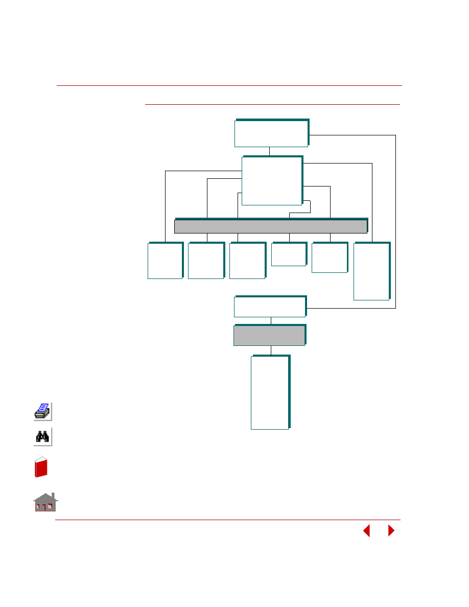
Overview of Commands for Design Optimization
and Sensitivity
The following figure provides an overview of commands required for defining
design variables, objective function, constraints, response quantities, and
optimization/sensitivity options in COSMOSM.
For more information on the commands, please refer to the COSMOSM Command
Reference manual (Volume 2).
Is required
number of runs
executed?
Yes
Perform Analysis
Update Geometry and
Mesh (If Needed)
De fine
S e nsitivity
P arame te rs
S e nsitivity Loop
Design
Parameters
(Variables)
Response
Quantities
Sensitivity
Types
•
•
•
P re proce ssing
Build Geometry and
Mesh in Terms of
Design Parameters
P e rform Analysis
P ostproce ssing
Deformed Shapes
Contour and
Vector Plots
X-Y Plots
Mode Shapes
Animation
•
•
•
•
•
Static
Frequency
Buckling
Thermal
Nonlinear
Post Dynamic
Dynamic Stress
Fatigue
•
•
•
•
•
•
•
•
No
In
de
x
In
de
x
Chapter 3 Procedures and Examples
3-4
COSMOSM Advanced Modules
Figure
3-3. Overview of Commands for Design Optimization and Sensitivity
DE S IGN O P TIMIZATIO N
AND S E NS ITIV ITY
• Design Variables
• Optimization Objective
• Optimization Constraints
• Sensitivity Response
• Optimization Loops
• Sensitivity Runs
ANALY S I S > O P TI MI ZE / S E NS I TI V I TY ME NU TRE E
CONVERGENCE AND
SENSITIVITY PLOTS
DI S P LAY > X Y _
P LO TS
ME NU TRE E
INITXYPLOT
ACTXYPOST
SETXYPLOT
XYRANGE
XYREFLINE
XYIDENTIFY
XYLIST
XYPTLIST
XYPLOT
DVARDEF
DVARLIST
DVARVDEL
OP_DVMOVE
SN_SETDEF
SN_SETLIST
SN_SETDEL
OP_CONDEF
OP_CONLIST
OP_CONDEL
OP_CONTRIM
OP_OBJDEF
OP_OBJSET
OP_OBJLIST
OP_OBJDEL
SN_RESPDEF
SN_RESPLIST
SN_RESPDEL
A_SENSITIV
R_SENSITIV
OP_CONTROL
OP_RESTORE
A_OPTIMIZE
R_OPTIMIZE
In
de
x
In
de
x
COSMOSM Advanced Modules
3-5
Part 2 OPSTAR / Optimization
Procedures for Performing Design Optimization
The following steps are recommended to be followed for performing design
optimization studies using OPTSTAR. These guidelines are not in any sense
complete, and are intended to be complementary to your own optimization
knowledge and expertise.
Step 1. Build the model parametrically
•
For shape optimization problems, build the model geometry parametrically in
places where it is necessary. For sizing optimization, the section constants (e.g.,
cross-sectional area of a truss) and design aspects to be optimized will be
defined as parameters. These parameters should then be defined as design
variables using the
DVARDEF
(Analysis > OPTIMIZE/SENSITIVITY >
DESIGN VARIABLES >
Define
) command. You may choose to use all or some
of the defined parameters in the optimization process. Note that the
DVARDEF
(Analysis > OPTIMIZE/SENSITIVITY > DESIGN VARIABLES >
Define
)
command needs to be applied to each design variable separately.
•
For design optimization and sensitivity, you need to use the COSMOSM
command language to parametrically model the design geometry and/or
physical properties. The command language essentially facilitates you to
describe the design variables in GEOSTAR for a fully automated design
optimization and sensitivity processes. Some of the capabilities of this
parametric language are:
- the use of single parameters, arrays and functions,
- construction of arithmetic expressions,
- generating macros,
- control structure commands, and
- logical expressions.
In most cases only the
PARASSIGN
(Control > PARAMETER >
Assign
Parameter
) command needs to be used. Refer to COSMOSM User Guide, Vol-
ume 1, Appendix E for more details.
•
You must exercise caution when using parameters to describe the model
geometry. The chosen parameters have to define the model completely so that
when their values are modified during the optimization loops, the geometry
creation and meshing will not fail.
In
de
x
In
de
x

Chapter 3 Procedures and Examples
3-6
COSMOSM Advanced Modules
Step 2. Execute required initial analyses
•
Execute the initial analysis as usual in COSMOSM. The types of analyses
currently supported for design optimization are:
- linear static stress analysis (including multiple load cases),
- linearized buckling analysis,
- analysis of natural frequencies and mode shapes,
- heat transfer analysis,
- nonlinear structural analysis,
- post dynamic analysis,
- dynamic stress analysis, and
- fatigue analysis.
•
For multidisciplinary design optimization, you can execute the analyses in any
order before proceeding with optimization loops except the following cases.
•
It should be noted that natural frequency analysis and buckling analysis cannot
be combined in a multidisciplinary optimization application since they share the
same database locations in the program unless user-defined postprocessing
functions are used for constraints and/or objective functions.
•
If you are performing design optimization on a heat transfer - linear static
problem in which the temperatures are computed using either HSTAR or FFE
Thermal, then you need to follow the procedure listed below in order to input
the heat transfer results as thermal loads in static analysis:
- Use
R_THERMAL
(Analysis > HEAT TRANSFER >
Run Thermal Analysis
)
command to execute heat transfer analysis.
- Use
TEMPREAD
(LoadsBC > LOAD OPTIONS >
Read Temp as Load
)
command to read temperatures from heat transfer analysis.
- Use
A_STATIC
(Analysis > STATIC >
Static Analysis Options
) command with
flag T to include thermal loading in static analysis.
- Use
R_STATIC
(Analysis > STATIC >
Run Static Analysis
) command to
execute linear static analysis.
•
Post dynamic and fatigue analyses cannot be executed alone instead they must
follow other types of analysis. You need to follow the procedures listed below to
get correct results.
- Post dynamic analysis:
1. Use
R_FREQUENCY
(Analysis > FREQUENCY/BUCKLING >
Run
Frequency
) command to execute analysis of natural frequencies and mode
shapes,
In
de
x
In
de
x

COSMOSM Advanced Modules
3-7
Part 2 OPSTAR / Optimization
2. Use
R_DYNAMIC
(Analysis > POST-DYNAMIC >
Run Post Dynamic
)
command to execute post dynamic analysis,
3. Use
R_STRESS
(Analysis > STATIC >
Run Stress Analysis
) command to
execute dynamic stress analysis if desired.
- Fatigue analysis:
1. Use
R_STATIC
(Analysis > STATIC >
Run Static Analysis
) or
R_NONLINEAR
(Analysis > NONLINEAR >
Run NonL Analysis
)
command to execute linear or nonlinear structural analysis respectively or
R_FREQUENCY
(Analysis > FREQUENCY/BUCKLING >
Run
Frequency
),
R_DYNAMIC
(Analysis > POST-DYNAMIC >
Run Post
Dynamic
),
and
R_STRESS
(Analysis > STATIC >
Run Stress Analysis
)
commands to execute frequency, post dynamic and dynamic stress analysis,
2. Use
R_FATIGUE
(Analysis > FATIGUE >
Run Fatigue Analysis
)
command to execute fatigue analysis.
Step 3. Perform postprocessing of initial analysis results
Perform postprocessing of the initial executed analyses as usual. For multi-
disciplinary analysis, you need to first activate the required type of analysis. Users
will have access to all existing GEOSTAR'S postprocessing features. Please refer to
User Guide (Vol. 1) and Basic FEA System Manual (Vol. 3) for more information.
Step 4. Begin design optimization procedures by defining design
variables
•
First, define the design variables using the command
DVARDEF
(Analysis >
OPTIMIZE/SENSITIVITY > DESIGN VARIABLES >
Define
). Note that each
design variable, whether in shape or sizing optimization, must have already been
defined as a parameter [using the
PARASSIGN
(Control > PARAMETER >
Assign Parameter
) command]. The command controls the following
information:
- Type of variable (shape or sizing) and its parametric name,
- Lower and upper bounds,
- Convergence tolerance (see Chapter 4),
Default values = 1/100 | upper bound- to lower bound |
- Method of choosing the pre-optimization design variable values (perturbation
or random evaluation),
In
de
x
In
de
x

Chapter 3 Procedures and Examples
3-8
COSMOSM Advanced Modules
- Sizing options and element type (only for linear static analysis) where a
distinction has to be made between 2D and 3D beam elements and either
membrane or bending dominant behavior has to be indicated for shell
elements.
•
Use the commands
DVARDEL
(Analysis > OPTIMIZE/SENSITIVITY >
DESIGN VARIABLES >
Delete
) and
DVARLIST
(Analysis > OPTIMIZE/
SENSITIVITY > DESIGN VARIABLES >
List
) ‘to delete and list the design
variables respectively.
•
Use the commands
OP_DVMOVE
(Analysis > OPTIMIZE/SENSITIVITY >
DESIGN VARIABLES >
Move Limits
) to control the move limits of design
variables during the optimization loops. This command is seldom necessary
since its default options will suffice in most cases. Chapter 4, Numerical
Aspects explains in more detail how the move limits of design variables
function in each optimization loop.
Step 5. Define objective function
•
Define the objective function using the
OP_OBJDEF
(Analysis > OPTIMIZE/
SENSITIVITY > OBJECTIVE FUNCTION >
Define Function
) command.
The command controls the following information:
- Types of objective functions,
- Layer and face numbers (for composite shells only),
- Analysis type (for multidisciplinary optimization),
- Type of application (minimization or maximization),
- Criterion and approximation type (see Chapter 4),
- Convergence tolerance (see Chapter 4),
- Reference keypoint (relative displacement),
- Load case (multiple load cases only) or time step number (nonlinear or post
dynamic only).
•
You can use the
OP_OBJSET
(Analysis > OPTIMIZE/SENSITIVITY >
OBJECTIVE FUNCTION >
Define Function Set
) command to declare
portions (sets) of the model for objective function computations. It is also
possible to assign weight factors to different parts of the model using the same
command. This command is most useful for volume and weight objective
functions (cost). However, it cannot be used with frequency and buckling
functions.
In
de
x
In
de
x

COSMOSM Advanced Modules
3-9
Part 2 OPSTAR / Optimization
•
Use the
OP_OBJDEL
(Analysis > OPTIMIZE/SENSITIVITY > OBJECTIVE
FUNCTION >
Del Function Set
) command to delete sets defined by the
OP_OBJSET
(Analysis > OPTIMIZE/SENSITIVITY > OBJECTIVE
FUNCTION >
Define Function Set
) command.
•
To delete the objective function defined using the
OP_OBJDEF
(Analysis >
OPTIMIZE/SENSITIVITY > OBJECTIVE FUNCTION >
Define Function
)
command, you need to use the same command again to overwrite the old
information.
•
Use the
OP_OBJLIST
(Analysis > OPTIMIZE/SENSITIVITY > OBJECTIVE
FUNCTION >
List Function
) command to list information defined by
OP_OBJDEF
(Analysis > OPTIMIZE/SENSITIVITY > OBJECTIVE
FUNCTION >
Define Function
) and
OP_OBJSET
(Analysis > OPTIMIZE/
SENSITIVITY > OBJECTIVE FUNCTION >
Define Function Set
)
commands.
Step 6. Define constraints
•
Define behavior constraints using the
OP_CONDEF
(Analysis > OPTIMIZE/
SENSITIVITY > BEHAVIOR CONSTRAINT >
Define
) command. The
command controls the following information:
- Types of behavior constraints,
- Layer and face numbers (for composite shells only),
- Analysis type (for multidisciplinary optimization),
- Geometry association,
- Lower and upper limits (bounds),
- Feasibility tolerance:
Default values = 1/100 | upper bound- to lower bound |
- Reference keypoint (relative displacement),
- Criterion and approximation type (see Chapter 4),
- Load case (multiple load cases only) or time step number (nonlinear or post
dynamic only).
•
Use
OP_CONLIST
(Analysis > OPTIMIZE/SENSITIVITY > BEHAVIOR
CONSTRAINT >
List Behavior Const
) and
OP_CONDEL
(Analysis >
OPTIMIZE/SENSITIVITY > BEHAVIOR CONSTRAINT >
Del Behavior
Const
) commands to list and delete constraints, respectively.
In
de
x
In
de
x

Chapter 3 Procedures and Examples
3-10
COSMOSM Advanced Modules
•
By default, OPTSTAR considers only the violated and potentially critical
constraints during calculations. In order to control this step, use the command
OP_CONTRIM
(Analysis > OPTIMIZE/SENSITIVITY > BEHAVIOR
CONSTRAINT >
Truncate Constraint
) which allows you to input trimming
(truncation) factors for the unviolated constraints. If the normalized value of a
particular constraint is above the negative value of the truncation factor, then
that constraint is appended to the critical list. For more detailed explanation,
refer to Chapter 4, Numerical Aspects.
Step 7. Specify parameters for optimization
•
Specify the parameters for the optimization loops using the
A_OPTIMIZE
(Analysis > OPTIMIZE/SENSITIVITY > OPTIMIZE LOOP >
Optimize
Analysis Options
) command. The important input for this command are:
– Maximum number of optimization loops (nloops flag)
– Number of stages to check convergence (loop_conv flag)
– Type of analyses. It should be mentioned that an optimization loop will
execute the analyses in the same sequence specified here. For heat transfer -
linear static problems requiring data transfer from heat transfer to static
analysis, you must specify THERMAL followed by STATIC.
– Number of consecutive infeasible design sets. You are recommended to
always start with a feasible initial design. Otherwise, the program will prompt
you with a choice to continue or stop. If you choose to continue, the
optimization loops will be terminated if a feasible solution is not reached after
five consecutive attempts. To change this number (five), use the
A_OPTIMIZE
(Analysis > OPTIMIZE/SENSITIVITY > OPTIMIZE LOOP >
Optimize
Analysis Options
) command and specify the appropriate input for the infeas
flag.
•
Start the optimization process using the
R_OPTIMIZE
(Analysis > OPTIMIZE/
SENSITIVITY > OPTIMIZE LOOP >
Run Optimize Analysis
) command.
Step 8. Restart options prior to convergence
In cases where the maximum number of optimization loops are exceeded, you can
restart the process by activating the restart flag under the
A_OPTIMIZE
(Analysis >
OPTIMIZE/SENSITIVITY > OPTIMIZE LOOP >
Optimize Analysis Options
)
command, followed by the
R_OPTIMIZE
(Analysis > OPTIMIZE/SENSITIVITY >
OPTIMIZE LOOP >
Run Optimize Analysis
) command. If you choose to use this
option, only the following commands can be reissued (if needed):
DVARLIST
,
OP_DVMOVE
,
OP_CONLIST
,
OP_CONTRIM
,
OP_OBJLIST
,
OP_CONTROL
.
In
de
x
In
de
x

COSMOSM Advanced Modules
3-11
Part 2 OPSTAR / Optimization
Step 9. Postprocess optimization results
•
You can display convergence plots of objective function (component name
OP_OBJ), behavior constraints (component name OP_CON), and design
variables (component name OP_DVAR) against number of loops using the
ACTXYPOST
(Display > XY PLOTS >
Activate Post-Proc
) and
XYPLOT
(Display > XY PLOTS >
Plot Curves
) commands from the Display-XY Plots
menu tree. It is also possible to list the activated result component on-line using
the
XYPTLIST
(Display > XY PLOTS >
List Points
) command. It should be
mentioned that the
ACTPOST
(Results > SET UP >
Set PostProcess Type
)
command has to be used prior to using the
ACTXYPOST
(Display > XY PLOTS
>
Activate Post-Proc
) command.
•
The optimization results for each loop are summarized in the output file
jobname.OPT.
Step 10. Postprocess converged analyses results
•
Perform postprocessing of the converged analyses as usual. Please refer to User
Guide (Vol. 1) and Basic FEA System Manual (Vol. 3) for more information.
•
One of the good features of the optimization module is that you will have the
optimum product in terms of its geometric dimensions (not giving only the final
coordinates of the mesh) which is an aspect favored in the manufacturing
process. Using the standard methods of transferring geometry (such as IGES
and DXF formats), the users can transfer the final geometry to NC machines.
Step 11. Restore an interim design set
•
It is possible to examine the design configuration at an interim step even after
the convergence of the optimization loops. The command
OP_RESTORE
(Analysis > OPTIMIZE/SENSITIVITY > OPTIMIZE LOOP >
Restore
Design Set
) can be used to restore a design set (corresponding to a specified
loop number) so that the entire database can be reconstructed for the specified
design set and the required analyses run automatically.
•
If you use the
OP_RESTORE
(Analysis > OPTIMIZE/SENSITIVITY >
OPTIMIZE LOOP >
Restore Design Set
) command, note that the converged
solution obtained will be lost. You need to therefore save the database of the
converged solution before applying this command.
In
de
x
In
de
x
Chapter 3 Procedures and Examples
3-12
COSMOSM Advanced Modules
Procedures for Performing Sensitivity Studies
The following steps are recommended to be followed for performing sensitivity
studies using OPTSTAR. These guidelines are not in any sense complete, and are
intended to be complementary to your own knowledge and experience.
Step 1. Initial model and analysis
The first step is similar to steps 1 through 3 of the procedures recommended for
performing design optimization:
–
Build the model parametrically
–
Execute required initial analyses
–
Perform postprocessing of initial analysis results
Step 2. Begin sensitivity study by defining design variables
•
Define the design variables using the
DVARDEF
(Analysis > OPTIMIZE/
SENSITIVITY > DESIGN VARIABLES >
Define
) command. Note that each
design variable, whether of shape of sizing type, must have been already defined
as a parameter (using the
PARASSIGN
(Control > PARAMETER >
Assign
Parameter
) command). It should be noted that the
DVARDEF
(Analysis >
OPTIMIZE/SENSITIVITY > DESIGN VARIABLES >
Define
) command is
used for both optimization and sensitivity applications where some options of
the command are needed only for optimization.
•
Use the commands
DVARDEF
(Analysis > OPTIMIZE/SENSITIVITY >
DESIGN VARIABLES >
Define
) and
DVARLIST
(Analysis > OPTIMIZE/
SENSITIVITY > DESIGN VARIABLES >
>
List
) to delete and list the design
variables respectively.
Step 3. Define the sensitivity response quantities
•
Define the response quantity using the
SN_RESPDEF
(Analysis > OPTIMIZE/
SENSITIVITY > RESPONSE QUANTITY >
Define
) command. The
commands controls the following information:
- Type of response quantities,
- Layer and face numbers (for composite shells only),
- Analysis type (for multidisciplinary optimization),
- Geometry association,
In
de
x
In
de
x

COSMOSM Advanced Modules
3-13
Part 2 OPSTAR / Optimization
- Reference keypoint (relative displacement),
- Criterion type (see Chapter 4),
- Load case (multiple load cases only) or time step number (nonlinear or post
dynamic only).
•
Use
SN_RESPDEL
(Analysis > OPTIMIZE/SENSITIVITY > RESPONSE
QUANTITY >
Delete
) and
SN_RESPLIST
(Analysis > OPTIMIZE/
SENSITIVITY > RESPONSE QUANTITY >
List
) to delete and list response
quantities respectively.
Step 4. Specify type of sensitivity
•
Specify the type and parameters of the sensitivity study using the
A_SENSITIV
(Analysis > OPTIMIZE/SENSITIVITY > SENSITIVITY RUN >
Options
)
command. The important input for this command are:
– Type of sensitivity:
•
Global sensitivity, offset sensitivity, or local sensitivity. For offset and local
sensitivity studies, the command
SN_SETDEF
(Analysis > OPTIMIZE/
SENSITIVITY > RESPONSE QUANTITY >
Define
) should be used to
define the user-specified design sets.
– Type of analyses:
•
It should be mentioned that a sensitivity run will execute the analyses in the
same sequence specified here. For instance if you want to find the fundamental
frequency of the model based on the deformed configuration calculated by the
nonlinear program, you must specify NONLINEAR followed by
FREQUENCY.
•
Start the sensitivity study by using the
R_SENSITIV
(Analysis > OPTIMIZE/
SENSITIVITY > SENSITIVITY RUN >
Run Analysis
) command.
Step 5. Restart option
In cases where the sensitivity study is terminated by the user or due to an error, you
can restart the process by activating the restart flag under the
A_SENSITIV
(Analysis > OPTIMIZE/SENSITIVITY > SENSITIVITY RUN >
Options
)
command, followed by the
R_SENSITIV
(Analysis > OPTIMIZE/SENSITIVITY >
SENSITIVITY RUN >
Run Analysis
) command.
In
de
x
In
de
x
Chapter 3 Procedures and Examples
3-14
COSMOSM Advanced Modules
Step 6. Postprocess sensitivity results
•
You can display plots of response quantities against value or label of design
variables using the
ACTXYPOST
(Display > XY PLOTS >
Activate Post-Proc
)
and
XYPLOT
(Display > XY PLOTS >
Plot Curves
) commands from the
Display-XY Plots menu tree. It is also possible to list the activated result
component on-line using the
XYPTLIST
(Display > XY PLOTS >
List Points
)
command. It should be mentioned that the
ACTPOST
(Results > SET UP >
Set
PostProcess Type
) command has to be used prior to using the
ACTXYPOST
(Display > XY PLOTS >
Activate Post-Proc
) command.
•
The sensitivity results are summarized in the output file jobname.OPT.
Special Features for Optimization and Sensitivity
Dynamic change of parameters
The user can specify the flags controlling the optimization and sensitivity features in
terms of parametric expressions. For example, the upper and lower bounds of a
design variable may not always be a constant value but depends on some boundary
conditions and geometric features that change from one optimization or sensitivity
run to another.
Restart option
•
For optimization, users can restart the process from the last successful design
sets in the following cases:
– Iterations exceed the maximum allowed number.
– Number of trials to find a feasible solution exceeds the allowed number.
– Optimization process terminated by the user either during the optimization
screen or during regenerating the model's geometry or mesh using the <Esc>
key
– Optimization terminated because of failure to regenerate the model or crash of
optimization procedure.
•
For sensitivity studies, you can restart the process from the last successful run in
the following cases:
- Terminating the process during the sensitivity screen or generating the model's
geometry or mesh using the <Esc> key.
- Failure to regenerate the model.
In
de
x
In
de
x

COSMOSM Advanced Modules
3-15
Part 2 OPSTAR / Optimization
•
It should be mentioned that you can restart the optimization process (as a fresh
start) from the current design variable values as new initial values by choosing
the OFF option in the restart flag. In this case, optimization will begin its first
iteration all over again. For example, if your model converged to an optimum
selection in eight iterations, and you chose to restore the fifth design set to
inspect it. If you choose fresh start at this point, the optimizer will consider the
design variables, constraints and objective function values of the fifth design set
as initial values in a new optimization run.
User-defined constraints, objective function and sensitivity response
quantities
•
Situations may arise where you need to customize your own objective function,
behavior constraints, or sensitivity response quantities. A user-defined feature is
included in the
OP_OBJDEF
(Analysis > OPTIMIZE/SENSITIVITY >
OBJECTIVE FUNCTION >
Define Function
),
OP_CONDEF
(Analysis >
OPTIMIZE/SENSITIVITY > BEHAVIOR CONSTRAINT >
Define Behavior
Constraint
) and
SN_RESPDEF
(Analysis > OPTIMIZE/SENSITIVITY >
RESPONSE QUANTITY >
Define
) commands. The user-defined quantity has
to be declared by a
PARASSIGN
(Control > PARAMETER >
Assign
Parameter
) command prior to issuing the
OP_OBJDEF
(Analysis >
OPTIMIZE/SENSITIVITY > OBJECTIVE FUNCTION >
Define Function
),
OP_CONDEF
(Analysis > OPTIMIZE/SENSITIVITY > BEHAVIOR
CONSTRAINTS >
Define Behavior Constraint
) or
SN_RESPDEF
(Analysis >
OPTIMIZE/SENSITIVITY > RESPONSE QUANTITY >
Define
) commands.
These quantities can be calculated using the extensive options provided by the
COSMOSM command language (User Guide, Vol. 1, Appendix E).
•
Regenerating the model through GEOSTAR requires reading all the steps you
followed as stored in the session file in every optimization or sensitivity loop.
There are however some commands (action commands) in the session file that
are ignored by GEOSTAR (e.g. “
R_
” or “
R...
” commands). The reason is that it
would be very time consuming to follow the user's steps of running analysis
modules since you might have executed these commands many times to check
and modify the initial model. Instead, the control of this step is left to the
A_OPTIMIZE
(Analysis > OPTIMIZE/SENSITIVITY > OPTIMIZE LOOP >
Optimize Analysis Options
) and
A_SENSITIV
(Analysis > OPTIMIZE/
SENSITIVITY > SENSITIVITY RUN >
Options
) commands.
In
de
x
In
de
x

Chapter 3 Procedures and Examples
3-16
COSMOSM Advanced Modules
•
User-defined objective function, behavior constraint or a response quantity may
be a preprocessing or a postprocessing quantity. An example of a preprocessing
quantity is the volume or weight of some elements. Once the mesh is generated
you will be able to use its information to calculate these quantities (using
VOLUME and WEIGHT functions explained in Appendix E of the User
Guide.) If the user-defined feature is a postprocessing-function dependent
quantity, it must be defined after running the analysis. For example, in order to
use the frequency function (FREQ) you have to execute
R_FREQUENCY
(Analysis > FREQUENCY/BUCKLING >
Run Frequency
) first. Another
example is the use of secondary load cases using the
LCCOMB
(Results >
Combine Load Case
) command. You need to run
R_STATIC
(Analysis >
STATIC >
Run Static Analysis
first followed by the
LCCOMB
(Results >
Combine Load Case
) command.
•
In order to respect the sequence (or order) of issuing some of GEOSTAR
commands which is essential in some user-defined cases, a separate option is
included in the type of analysis flag defined by the
A_OPTIMIZE
(Analysis >
OPTIMIZE/SENSITIVITY > OPTIMIZE LOOP >
Optimize Analysis
Options
) and
A_SENSITIV
(Analysis > OPTIMIZE/SENSITIVITY >
SENSITIVITY RUN >
Options
) command. This option is called “FILE”, and it
means that the type of analysis (“
R_
” commands.) and other GEOSTAR
commands are included in a separate file prepared by the user. The file name
should be GEOFILE.FIL and it has to be located in the local directory. This file
include the “
R_
”
commands and other action commands given in the sequence
necessary for calculating the user-defined quantities.
In
de
x
In
de
x
COSMOSM Advanced Modules
3-17
Part 2 OPSTAR / Optimization
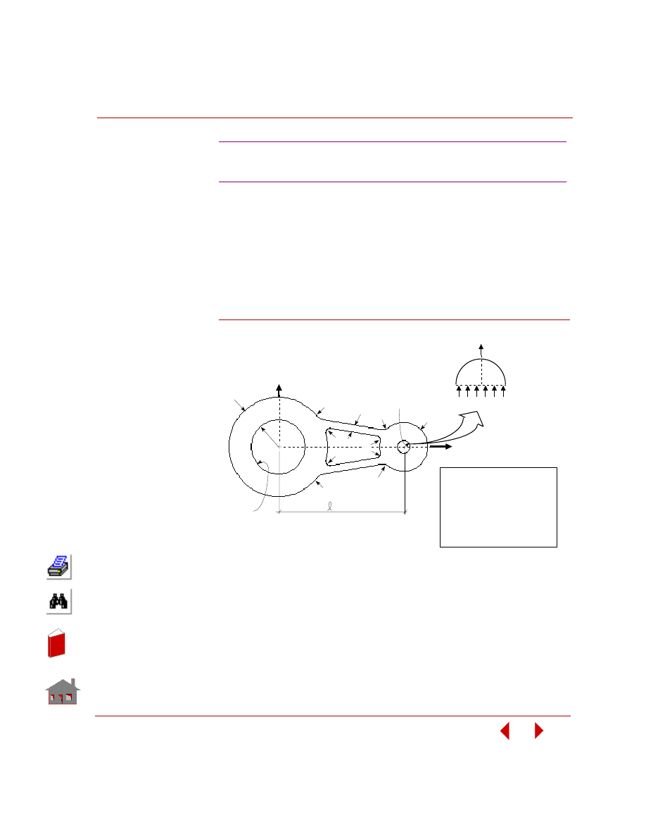
In this example, you are required to find the thickness of the two shafts (TR1 and
TR2), and the size and location of the cutout (TW). The outer arm thickness is 20
mm, modulus of elasticity is 2 x 10
5
MPa, and Poisson’s ratio is 0.3. The control
arm is subjected to a pressure loading of 4 MPa as shown in the following figure.
The only constraint on the control arm is that the von Mises stress due to the
applied loading should neither exceed 225 MPa nor fall below 10 MPa. The
objective function for minimization is the volume of the control arm with a
tolerance of 1%.
Figure
3-4. Initial Geometry, Boundary Conditions and Loads
The design variables for this problem as seen from the above figure are
designated as TR1, TR2 and TW. Since their value will change with each
optimization cycle, they will be defined as parameters using the
PARASSIGN
(Control > PARAMETER >
Assign Parameter
) command. The bounds, initial
values and tolerances for the design variables are as shown below:
Shape Optimization of a Slotted
Control Arm in Static Analysis
5
5
5
tr
Fixed
= 140
1
tr
2
20
20
10
10
tw
P
Y
6 - Node TRI ANG
= 20 mm
= 2 x 10 N/mm
2
5
= 0.3
= 4 N/ mm
(Y direction)
Thickness
E
Note: All dimensions in millimeters.
ν
2
P
r = 30
1
r = 7
2
Y
X
y
y
In
de
x
In
de
x
Chapter 3 Procedures and Examples
3-18
COSMOSM Advanced Modules
Using the design variables as well as other geometric dimensions, you will first
build the initial geometry of the model parametrically. In the next step, the finite
element mesh of the initial geometry will be subjected to loads and boundary
conditions. The linear static stress analysis is performed as usual. After successful
completion, you need to specify the input for design optimization, and solve for the
optimal shape of the control arm. During the optimization cycle, the program will
automatically change the design variable values as required and perform linear
static stress analysis to satisfy the constraints. The following paragraphs describe
all relevant steps in detail with illustrations.
1.
To start with, set a working plane by executing the following command:
Geo Panel:
Geometry > GRID >
Plane (PLANE)
Rotation/sweep axis >
2
Offset on axis >
0.0
Grid line style >
Solid
2.
Initialize all parameters used to build the model using the
PARASSIGN
(Control
> PARAMETER >
Assign Parameter
) command. Let us start with the design
variables (TR1, TR2 and TW):
Geo Panel:
Control > PARAMETER >
Assign Parameter (PARASSIGN)
Parameter name >
TR1
Data type >
REAL
Parametric real value >
25
Geo Panel:
Control > PARAMETER >
Assign Parameter
(PARASSIGN)
Parameter name >
TR2
Data type >
Real
Parameter real value >
20
In addition to the required design variables, you can define some other
dimensions of the model as parameters. These dimensions include the length
between the centers of the shafts and their radii (L, R1 and R2).
Bounds
Initial Value
Tolerance
8
≤
TR1
≤
25
25
1
8
≤
TR2
≤
20
20
1
3
≤
TW
≤
8
8
0.5
In
de
x
In
de
x
COSMOSM Advanced Modules
3-19
Part 2 OPSTAR / Optimization
Geo Panel:
Control > PARAMETER >
Assign Parameter
(PARASSIGN)
Parameter name >
R1
Data type >
Real
Parameter real value >
30
Geo Panel:
Control > PARAMETER >
Assign Parameter (PARASSIGN)
Parameter name >
R2
Data type >
Real
Parameter real value >
7
Geo Panel:
Control > PARAMETER >
Assign Parameter (PARASSIGN)
Parameter name >
L
Data type >
Real
Parameter real value >
140
The parameters defined above can be listed on-screen using the
PARLIST
(Control > PARAMETER >
List Parameter
) command which provides a
summary as shown below:
3.
For this problem, you need to increase the closure tolerances at keypoints.
Establish keypoints for the centers of shafts as follows (note the parametric
input for the center of the smaller shaft):
Geo Panel:
Geometry > POINTS >
Merge Tolerance (PTTOL)
Tolerance >
0.001
Geo Panel:
Geometry > POINTS >
Define (PT)
Keypoint >
1
XYZ-coordinate value >
0.0, 0.0, 0.0
Geo Panel:
Geometry > POINTS >
Define (PT)
Keypoint >
2
XYZ-coordinate value >
L, 0, 0
Num
Name
Type
Value
1
TR1
REAL
25.000000
2
TR2
REAL
20.000000
3
TW
REAL
8.000000
4 R1
REAL
30.000000
5 R2
REAL
7.000000
6 L
REAL
140.000000
In
de
x
In
de
x

Chapter 3 Procedures and Examples
3-20
COSMOSM Advanced Modules
4.
Use the Auto scale icon to adjust the view on the screen. Next, draw circles at
the points created above using the
CRSCIRCLE
(Geometry > CURVES >
CIRCLES >
By Center/Edge
) command to model the two shafts. The shafts
have a radius of R1 and R2 with thickness of TR1 and TR2 (defined as
parameters). The prompts and input for creating the shafts are as below
[
ACTNUM
(Control > ACTIVATE >
Entity Label
) command is used to activate
labels of curves]:
Geo Panel:
Geometry > CURVES > CIRCLES >
By Center/Edge
(CRSCIRCLE)
Curve >
1
XYZ-coordinate value of center of circle >
0.0, 0.0, 0.0
XYZ-coordinate value of center of circle >
R1, 0.0, 0.0
Number of segments >
4
Geo Panel:
Geometry > CURVES > CIRCLES >
By Center/Edge
(CRSCIRCLE)
Curve >
5
XYZ-coordinate value of center of circle >
L, 0.0, 0.0
XYZ-coordinate value of center of circle >
L+R2, 0.0, 0.0
Number of segments >
4
Geo Panel:
Geometry > CURVES > CIRCLES >
By Center/Edge
(CRSCIRCLE)
Curve >
9
XYZ-coordinate value of center of circle >
0.0, 0.0, 0.0
XYZ-coordinate value of center of circle >
R1+TR1, 0.0, 0.0
Number of segments >
4
Geo Panel:
Geometry > CURVES > CIRCLES >
By Center/Edge
(CRSCIRCLE)
Curve >
13
XYZ-coordinate value of center of circle >
L
XYZ-coordinate value of center of circle >
L+R2+TR2
Number of segments >
4
5.
Use the Auto scale icon to re-scale the screen view. The circles created above
will be connected together by straight lines tangential to the inner circles of the
shafts using the
CRTANLIN
(Geometry > CURVES > MANIPULATION
MENU >
Tangent btwn 2 Cr
) command as illustrated below.
In
de
x
In
de
x
COSMOSM Advanced Modules
3-21
Part 2 OPSTAR / Optimization
Geo Panel:
Geometry > CURVES > MANIPULATION MENU >
Tangent
btwn 2 Cr (CRTANLIN)
Curve >
17
Curve 1 >
1
Curve 2 >
5
Break flag >
Do not break
Geo Panel:
Geometry > CURVES > MANIPULATION MENU >
Tangent
btwn 2 Cr (CRTANLIN)
Curve >
18
Curve 1 >
4
Curve 2 >
8
Break flag >
Do not break
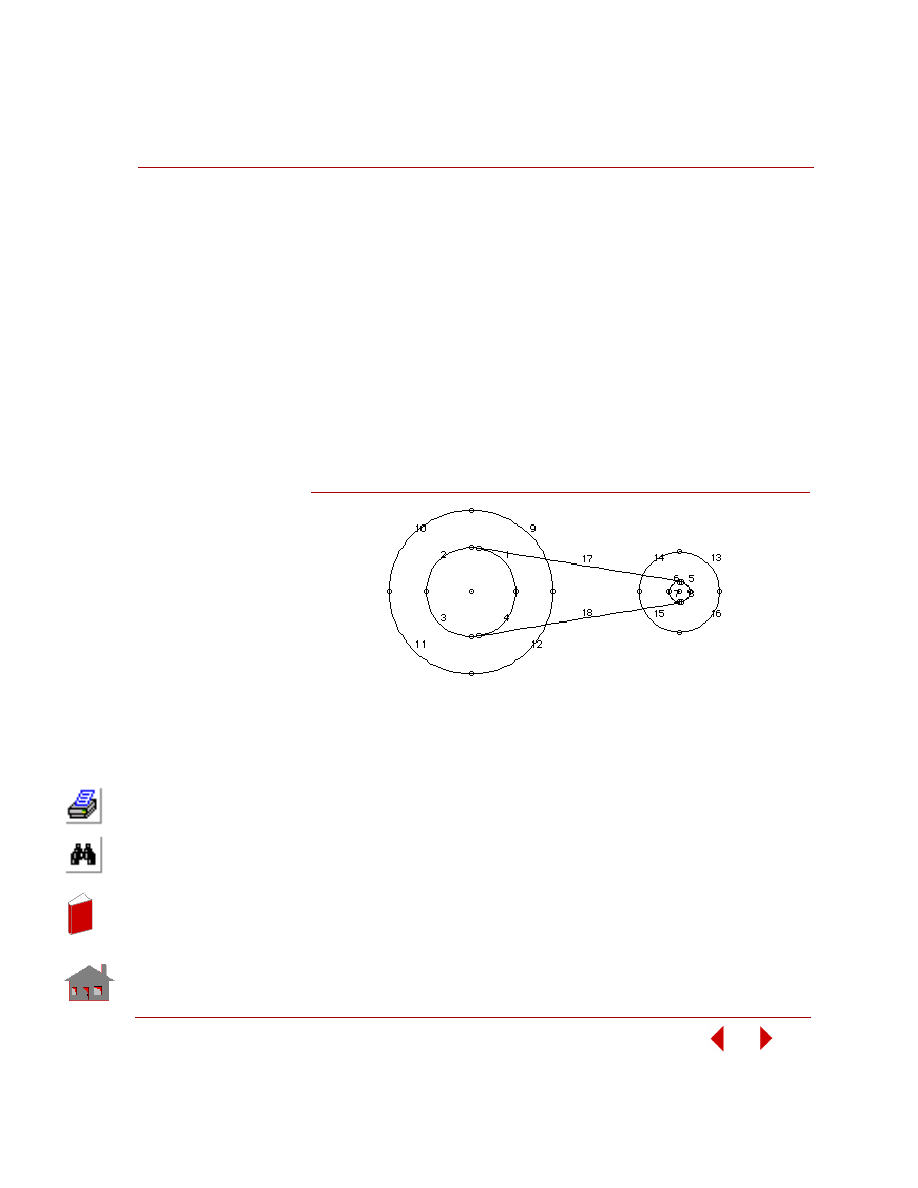
The figure below shows a view of the two shafts connected together by tangential
lines. Note that the lines protruding into the shaft thicknesses will be trimmed later.
Figure
3-5 Construction of Tangential Lines Connecting the Shafts
6.
Activate the display of point tables using the Status 1 icon. In the next step, you
will construct two more lines parallel to the tangents created earlier representing
the slotted portion of the model. In order to draw these lines, you can define a
coordinate system along the tangential lines so that the new curves generated
will be parallel to the tangential lines. Use the
CSYS
(Geometry > COORD
SYS >
By 3 Points
) command as shown below:
Geo Panel:
Geometry > COORD SYS >
By 3 Points (CSYS)
Coordinate system >
3
Coordinate system type >
Cartesian
Keypoint at origin >
19
Keypoint on the X-axis >
20
Keypoint on the X-Y plane >
1
In
de
x
In
de
x

Chapter 3 Procedures and Examples
3-22
COSMOSM Advanced Modules
Geo Panel:
Geometry > COORD SYS >
By 3 Points (CSYS)
Generation number >
1
Beginning curve >
18
Ending curve >
18
Increment <
1
Generation flag >
Translation
X-displacement >
0.0
Y-displacement >
-TW
Z displacement >
0.0
Next, apply the
CRGEN
(Geometry > CURVES > GENERATION MENU >
Generate
) command at the top tangent line and input an offset of -TW (with
respect to the new coordinate system) which represents the thickness of the
slotted portion.
Geo Panel:
Geometry > CURVES > GENERATION MENU >
Generate
(CRGEN)
Generation number >
1
Beginning curve >
17
Ending curve >
17
Increment >
1
Generation flag >
Translation
X-displacement >
0.0
Y-displacement >
-TW
Z-displacement >
0.0
Similarly apply the
CSYS
(Geometry > COORD SYS >
By 3 Points
) and
CRGEN
(Geometry > CURVES > GENERATION MENU >
Generate
)
commands at the bottom tangent line as shown below:
Geo Panel:
Geometry > COORD SYS >
By 3 Points (CSYS)
Coordinate system >
4
Coordinate system type >
Cartesian
Keypoint at origin >
21
Keypoint on the X-axis >
22
Keypoint on the X-Y plane >
1
7.
You now need to remove the lines protruding into the shaft thicknesses. This can
be achieved by finding the intersection of the straight lines with the outer circles
of the shafts and then subdividing the lines at the points of intersection. The
lines inside the shafts can be then easily removed. The commands below
illustrate these tasks:
In
de
x
In
de
x

COSMOSM Advanced Modules
3-23
Part 2 OPSTAR / Optimization
Geo Panel:
Geometry > POINTS > GENERATION MENU >
Cr/Cr
Intersect (PTINTCC)
Primary curve >
17
Beginning curve >
9
Ending curve >
14
Increment >
5
Tolerance >
0.000050
Geo Panel:
Geometry > CURVES > MANIPULATION MENU >
Break
Near Pt (CRPTBRK)
Curve to be broken >
17
Reference keypoint >
27
Original curve keeping flag >
Do not keep
Geo Panel:
Geometry > CURVES > MANIPULATION MENU >
Break
Near Pt (CRPTBRK)
Curve to be broken >
21
Reference keypoint >
28
Original curve keeping flag >
Do not keep
Geo Panel:
Edit > DELETE >
Curves (CRDEL)
Beginning curve >
17
Ending curve >
22
Increment >
5
You need to repeat the above procedure for the remaining three lines of the
slotted portion as outlined below: (Cryptic commands need to be typed in the
command window; however, the command paths are also shown.)
Geo Panel:
Geometry > POINTS > GENERATION MENU >
Cr/Cr Intersect (PTINTCC)
PTINTCC,18,12,15,3;
Geo Panel:
Geometry > CURVES > MANIPULATION MENU >
Break
Near Pt (CRPTBRK)
CRPTBRK,18,29,0;
CRPTBRK,22,30,0;
Geo Panel:
Edit > DELETE >
Curves (CRDEL)
CRDEL,18,18,1;
CRDEL,23,23,1;
Geo Panel:
Geometry > POINTS > GENERATION MENU >
Cr/Cr Intersect (PTINTCC)
PTINTCC,19,9,14,5;
In
de
x
In
de
x

Chapter 3 Procedures and Examples
3-24
COSMOSM Advanced Modules
Geo Panel:
Geometry > CURVES > MANIPULATION MENU >
Break
Near Pt (CRPTBRK)
CRPTBRK,19,31,0;
CRPTBRK,23,32,0;
Geo Panel:
Edit > DELETE >
Curves (CRDEL)
CRDEL,19,19,1;
CRDEL,24,24,1;
Geo Panel:
Geometry > POINTS > GENERATION MENU >
Cr/Cr Intersect (PTINTCC)
PTINTCC,20,12,15,3;
Geo Panel:
Geometry > CURVES > MANIPULATION MENU >
Break
Near Pt (CRPTBRK)
CRPTBRK,20,33,0;
CRPTBRK,24,34,0;
Geo Panel:
Edit > DELETE >
Curves (CRDEL)
CRDEL,20,20,1;
CRDEL,25,25,1;
8.
Next, it is necessary to remove arcs of the outer circles at the connection with
the slotted portion so that model domain is continuous. There are four such arcs
and the
CRPTBRK
(Geometry > CURVES > MANIPULATION MENU >
Break Near Pt
) and
CRDEL
(Edit
>
DELETE
>
Curves
) commands are applied
to remove them as illustrated below:
Geo Panel:
Geometry > CURVES > MANIPULATION MENU >
Break
Near Pt (CRPTBRK)
CRPTBRK,9,27,0;
CRPTBRK,25,31,0;
Geo Panel:
Edit > DELETE >
Curves (CRDEL)
CRDEL,25,25,1;
Geo Panel:
Geometry > CURVES > MANIPULATION MENU >
Break
Near Pt (CRPTBRK)
CRPTBRK,12,29,0;
CRPTBRK,12,33,0;
Geo Panel:
Edit > DELETE >
Curves (CRDEL)
CRDEL,28,28,1;
In
de
x
In
de
x
COSMOSM Advanced Modules
3-25
Part 2 OPSTAR / Optimization
Geo Panel:
Geometry > CURVES > MANIPULATION MENU >
Break
Near Pt (CRPTBRK)
CRPTBRK,14,28,0;
CRPTBRK,14,32,0;
Geo Panel:
Edit > DELETE >
Curves (CRDEL)
CRDEL,29,29,1;
Geo Panel:
Geometry > CURVES > MANIPULATION MENU >
Break
Near Pt (CRPTBRK)
CRPTBRK,15,30,0;
CRPTBRK,29,34,0;
Geo Panel:
Edit > DELETE >
Curves (CRDEL)
CRDEL,29,29,1;
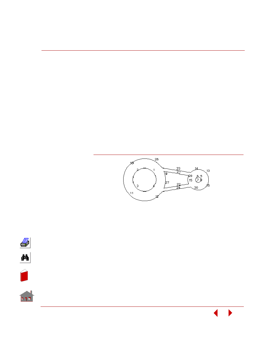
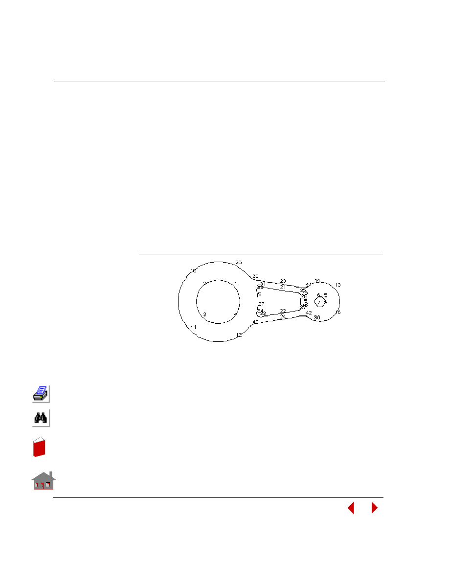
The figure below shows the geometry created so far, with curve labels activated.
These labels will be helpful in defining fillets at sharp corners, described next.
Figure
3-6. Interim Model Geometry with Curve Labels
9.
It is necessary to smooth the sharp corners at the intersection points of straight
lines with the shafts. Fillets at these points can be defined using the
CRFILLET
(Geometry > CURVES > MANIPULATION MENU >
Fillet
) command. The
labels of adjacent curves can be seen from the above figure for this command.
Geo Panel:
Geometry > CURVES > MANIPULATION MENU >
Fillet
(CRFILLET)
Curve >
31
Curve 1 >
21
Curve 2 >
9
Radius of fillet >
5
Trim flag >
Original curve keeping flag >
Tolerance >
0.000001
In
de
x
In
de
x
Chapter 3 Procedures and Examples
3-26
COSMOSM Advanced Modules
Repeat the above command at other locations as shown below (as before, the
cryptic commands need to be typed in the command window; command paths
on the menu are also shown):
Geo Panel:
Geometry > CURVES > MANIPULATION MENU >
Fillet
(CRFILLET)
CRFILLET,33,22,27,5,1,0;
CRFILLET,35,21,28,5,1,0;
CRFILLET,37,22,15,5,1,0;
CRFILLET,39,23,26,20,1,0;
CRFILLET,40,24,12,20,1,0;
CRFILLET,41,23,14,10,1,0;
CRFILLET,42,24,30,10,1,0;
The figure below shows the initial geometry of the control arm for finite element
model development. In order to generate the finite element mesh, you need to
convert the geometry to a region entity and use the automatic meshing feature for
regions.
Figure
3-7. Initial Geometry of the Control Arm for Finite Element Modeling
10.
There are four contours constituting one region entity for this model. The outer
contour will be designated as the first contour and the inner ones will be
numbered 2 through 4. The design variables TR1, TR2, and TW will alter the
profiles of the outer contour and the middle inner contour in the slotted portion.
The average element size is specified as half of the value of TW, the thickness of
the slotted part. You also need to switch to the global coordinate system at this
point. The contour and region definitions are illustrated below:
Geo Panel:
Control > ACTIVATE >
Set Entity (ACTSET)
Set Label >
CS
Coordinate system >
0
In
de
x
In
de
x

COSMOSM Advanced Modules
3-27
Part 2 OPSTAR / Optimization
Geo Panel:
Geometry > CONTOURS >
Define (CT)
Contour >
1
Mesh flag >
Esize
Average element size >
TW/2
Number of reference boundary curves >
1
Curve 1 >
23
Use selection set >
No
Geo Panel:
Geometry > CONTOURS >
Define (CT)
CT,2,0,TW/2,1,21,0;
CT,3,0,TW/2,1,1,0;
CT,4,0,TW/2,1,5,0;
Geo Panel:
Geometry > REGIONS >
Define (RG)
Region >
1
Number of contours >
1
Outer contour >
1
Inner contour 1 >
2
Inner contour 2 >
3
Inner contour 3 >
4
Underlying surface >
0
11.
Generate the finite element mesh and define the element group, material
properties, section constants, and higher order elements as illustrated below:
Geo Panel:
Propsets >
Element Group (EGROUP)
Element group >
1
Element Category >
Area
Element Type (for area) >
TRIANG
Accept defaults ....
Geo Panel:
Propsets >
Real Constant (RCONST)
Associated element group >
1
Real constant set >
1
Start location of the real constants >
1
No. of real constants to be entered >
2
RC1: thickness >
20
RC2: material angle (Beta) >
0.0
In
de
x
In
de
x

Chapter 3 Procedures and Examples
3-28
COSMOSM Advanced Modules
Geo Panel:
Propsets >
Material Property (MPROP)
Material property set >
1
Material property name >
EX
Property value >
200000
Material property name
NUXY
Property value >
0.3
Geo Panel:
Meshing > AUTO MESH >
Regions (MA_RG)
Beginning region >
1
Ending region >
1
Increment >
1
Number of smoothing iterations >
0
Method of Sweeping
Geo Panel:
Meshing > AUTO MESH >
Region
Mesh Type (MARGCH)
Beginning region >
1
Ending region >
1
Increment >
1
Element type >
T
Total element nodes >
6
Push flag >
Yes
Associate element group >
1
Define the boundary conditions and loads.
Geo Panel:
LoadsBC > STRUCTURAL > DISPLACEMENT >
Define
Curves (DCR)
Beginning curve >
1
Displacement label >
All
Value >
0.0
Ending curve >
4
Increment >
1
Geo Panel:
LoadsBC > STRUCTURAL > PRESSURE >
Define Curves
(PCR)
Beginning curve >
5
Pressure magnitude >
4
Ending curve >
6
Increment >
1
Pressure at the end of direction 1 >
4
Pressure direction >
Normal direction
In
de
x
In
de
x

COSMOSM Advanced Modules
3-29
Part 2 OPSTAR / Optimization
12.
Proceed with linear static stress analysis by executing the
R_STATIC
(Analysis
> STATIC >
Run Static Analysis
) command.
13.
It is a good practice to postprocess the results from the preliminary design
before starting the optimization loops due to several reasons. First, you can
eliminate any modeling errors by inspecting the results. More importantly, you
can make sure that the behavior constraints imposed on the model for
optimization are realistic. For this example, the von Mises stress constraint has
bounds of 10 and 225, whereas the computed von Mises stress for the
preliminary design ranges from 0 to 90 (you can either use the
STRMAX
(Results > EXTREMES >
Min/Max Stress
) or
STRPLOT
(Results > PLOT >
Stress
) commands to process the von Mises stress). Therefore, the constraints
specified for this example are indeed realistic.
After the linear static analysis is successfully completed, you can proceed to define
the input for shape optimization. The following commands for specifying
optimization analysis options are found in the Analysis > OPTIMIZE/
SENSITIVITY menu tree.
14.
Define the design variables. There are three design variables (TR1, TR2, and
TW) for this problem that will be applied in obtaining an optimal shape of the
model under linear static analysis. Each of the design variable needs to be
defined separately using the
DVARDEF
(Analysis > OPTIMIZE/SENSITIVITY
> DESIGN VARIABLES >
Define
) command. You also need to specify the
upper and lower bounds of the design variable under this command.
Geo Panel:
Analysis > OPTIMIZE/SENSITIVITY > DESIGN VARIABLES
>
Define (DVARDEF)
Design variable set number >
1
Design variable type >
Shape
Design variable parametric name >
TR1
Design variable lower bound >
8
Design variable upper bound >
25
Design variable conv. tol. for optimization >
1
Preopt process: zero=random nonzero=perturb_ratio >
0.0
Geo Panel:
Analysis > OPTIMIZE/SENSITIVITY > DESIGN VARIABLES
>
Define (DVARDEF)
Design variable set number >
2
Design variable type >
Shape
Design variable parametric name >
TR2
Design variable lower bound >
8
In
de
x
In
de
x
Chapter 3 Procedures and Examples
3-30
COSMOSM Advanced Modules
Design variable upper bound >
20
Design variable conv. tol. for optimization >
1
Preopt process: zero=random nonzero=perturb_ratio >
0.0
Geo Panel:
Analysis > OPTIMIZE/SENSITIVITY > DESIGN VARIABLES
>
Define (DVARDEF)
Design variable set number >
3
Design variable type >
Shape
Design variable parametric name >
TW
Design variable lower bound >
3
Design variable upper bound >
8
Design variable conv. tol. for optimization >
0.5
Preopt process: zero=random nonzero=perturb_ratio >
0.0
The
DVARLIST
(Analysis > OPTIMIZE/SENSITIVITY > DESIGN VARIABLES
>
List
) command can be used to obtain an on-screen listing of design variables
defined above. The listing for this problem is as shown below:
15.
The objective function to be minimized (or maximized) and the associated
parameters for nodal or elemental type functions is defined using the
OP_OBJDEF
(Analysis > OPTIMIZE/SENSITIVITY > OBJECTIVE
FUNCTION >
Define Function
) command. For this example, you will be
minimizing volume as an elemental quantity using linear approximation to start
with. Quadratic approximations with cross terms as well as cubic terms will be
used for subsequent approximations of the objective function (approximation
type 3).
Geo Panel:
Analysis > OPTIMIZE/SENSITIVITY> OBJECTIVE
FUNCTION >
Define Function (OP_OBJDEF)
Type >
Elemental
Objective >
Minimize
Elemental objective function name >
Volume
Set
Type
DvName
Value
Lower/
Upper Bound
Tolerance/
Perturb Ratio
1
Shape
TR1
2.5000e+001
8.0000e+000
1.0000e+000
2.5000e+001
0.0000e+000
2
Shape
TR2
2.0000e+001
8.0000e+000
1.0000e+000
2.0000e+001
0.0000e+000
3
Shape
TW
8.0000e+000
3.0000e+000
5.0000e-001
8.0000e+000
0.0000e+000
In
de
x
In
de
x

COSMOSM Advanced Modules
3-31
Part 2 OPSTAR / Optimization
Analysis type >
Linear
Unused option >
Unused option >
Objective function convergence tolerance (ratio) >
0.01
Objective function approximation type >
Linear + quadratic
The objective function input can be listed on-screen using the
OP_OBJLIST
(Analysis > OPTIMIZE/SENSITIVITY > OBJECTIVE FUNCTION >
List
Function
) command which provides the following information:
16.
The remaining input for performing shape optimization of the control arm
is the constraint definition. The
OP_CONDEF
(Analysis > OPTIMIZE/
SENSITIVITY > BEHAVIOR CONSTRAINT >
Define
) command is used
to define the constraints as illustrated below:
Geo Panel:
Analysis > OPTIMIZE/SENSITIVITY > BEHAVIOR
CONSTRAINT >
Define (OP_CONDEF)
Constraint set number >
1
Type >
Nodal
Nodal constraint name >
VON
Analysis type >
Linear
Criterion flag >
Max Abs
Layer number >
1
Face flag (shell) >
Top
Load case/time step >
1
Entity type assoc. with constraint >
Nodes
Beginning node >
1
Ending node >
NDMAX
See paragraph below
Increment of nodes >
1
Constraint lower bound >
10
Constraint upper bound >
225
Constraint feasibility tolerance >
3
Constraint approximation type >
Linear + Quad
Objtyp
= Elemental
Tolerance
= 1.000000e-002
Objname
= VOLUME
ApprxType
= 1
Objective
: Minimize
Value
= 2.003479e+005
Layer
= 1
Face
=1
Analysis
= Static
In
de
x
In
de
x

Chapter 3 Procedures and Examples
3-32
COSMOSM Advanced Modules
In the above, the second prompt seeks your input for the type of constraint, in
this case, nodal. The criterion flag specifies whether the absolute maximum, or
algebraic maximum, etc., is applied for evaluating the constraints. The entity
type associated with the constraint are nodes for this example. Since the label of
the ending node is not known in advance, and will keep changing for different
optimization loops, you can input a parametric equivalent (NDMAX) for that
prompt. The constraint upper and lower bounds as well as the tolerance are
input for the next three prompts. The last prompt seeks your input for constraint
approximation type. The default option of 1 for this prompt will use linear and
quadratic terms for approximations of the constraint function.
The constraint input can be listed on-screen using the
OP_CONLIST
(Analysis
> OPTIMIZE/SENSITIVITY > BEHAVIOR CONSTRAINT >
List Behavior
Const
) command.
17.
The last set of input you need to specify before beginning the optimization loops
is furnished using the
A_OPTIMIZE
(Analysis > OPTIMIZE/SENSITIVITY >
OPTIMIZE LOOP >
Optimize Analysis Options
) command. The command
and its input are shown below:
Geo Panel:
Analysis > OPTIMIZE/SENSITIVITY > OPTIMIZE LOOP >
Optimize Analysis Options (A_OPTIMIZE)
Maximum number of optimization loops >
10
Convergence check stages >
To the previous loop
No. of consec. infeasible designs >
5
Output print flag >
On
Echo option flag >
On
Restart flag >
Off
Type of analysis >
Static
In the above, the default option of 1 for the second prompt means that the
convergence is achieved if the change in the objective function and design
variables compared to the previous loop and the best design so far is less than
the tolerance. If the initial design is infeasible and your model goes through five
consecutive infeasible designs, the optimization process will be halted by
default. The type of analysis to be run in the optimization loop is static stress
analysis by default, and the program will prompt you further if you plan to run
multidisciplinary analyses. The options you specified under the
A_OPTIMIZE
(Analysis > OPTIMIZE/SENSITIVITY > OPTIMIZE LOOP >
Optimize
Analysis Options
) command can be listed on-screen using the
A_LIST
(Analysis >
List Analysis Option
) command (from the ANALYSIS submenu)
as shown below:
In
de
x
In
de
x
COSMOSM Advanced Modules
3-33
Part 2 OPSTAR / Optimization
Geo Panel:
Analysis >
List Analysis Option (A_LIST)
Component >
Optimization
18.
You can now proceed to perform the shape optimization analysis of the slotted
control arm. Use the
R_OPTIMIZE
(Analysis > OPTIMIZE/SENSITIVITY >
OPTIMIZE LOOP >
Run Optimize Analysis
) command to start the
optimization loops.
19.
The results of the static stress analysis performed will be written as usual to the
jobname.OUT file. Note that this file will only contain results corresponding to
the final design. If you want to store analysis results of all loops. you need to use
the
PRINT_OPS
(Analysis > OUTPUT OPTIONS >
Set Print Options
)
command to append all subsequent results to this file. For optimization iteration
summary of all loops, you can view the jobname.OPT file. Let’s create four
windows using
the New Win icon. Move to the first window by clicking inside
he window.
20.
In main window, we will plot the von Mises stresses using the
ACTSTR
and
STRPLOT
commands (Results > PLOT >
Stress
).
21.
In window 1, we will study the variation of objective functions versus the
optimization loops. Move to window 2 and execute the
ACTXYPOST
(Display
> XY PLOTS >
Activate Post-Proc
)
and
XYPLOT
(Display > XY PLOTS >
Plot Curves
) commands (Display > WINDOWS menu tree) as illustrated
below:
Geo Panel:
Results > SET UP >
Set to Post-Proc (ACTPOST)
Select optimization
Geo Panel:
Display > XY PLOTS >
Activate Post-Proc (ACTXYPOST)
Graph number >
1
Y_variable >
OP_OBJ
Type of results >
FEA
Graph color >
12
Graph line style >
Solid
Graph symbol style >
1
Graph id >
OP_OBJ
Adjust the X- and Y-axis intervals of the X-Y plot (for a clear display) by
making use of the
SETXYPLOT
(Display > XY PLOTS >
Set Plot Parameter
)
command as illustrated below:
In
de
x
In
de
x

Chapter 3 Procedures and Examples
3-34
COSMOSM Advanced Modules
Geo Panel:
Display > XY PLOTS >
Set Plot Parameter (SETXYPLOT)
X logarithmic >
No
Y logarithmic >
No
Number of X intervals >
7
Number of Y intervals >
4
Accept Defaults
Geo Panel:
Display > XY PLOTS >
Plot Curves (XYPLOT)
Plot graph 1 >
Yes
22.
In window 2, we will study the variation of the design variables versus the
optimization loops. Since there are three design variables in this example, you
will use set numbers 1, 2, and 3 for TR1 TR2 and TW respectively. Move to
window 3 and execute the
ACTXYPOST
(Display > XY PLOTS >
Activate
Post-Proc
)
and
XYPLOT
(Display > XY PLOTS >
Plot Curves
) commands as
illustrated below (remember to use the
SETXYPLOT
(Display > XY PLOTS >
Set Plot Parameter
) command to adjust the X-axis and Y-axis intervals):
Geo Panel:
Display > XY PLOTS >
Activate Post-Proc (ACTXYPOST)
Graph number >
1
Y_variable >
OP_DVAR
Set number >
1
Graph color >
12
Graph line style >
Solid
Graph symbol style >
1
Graph id >
OP_DVAR-1
Geo Panel:
Display > XY PLOTS >
Activate Post-Proc (ACTXYPOST)
Graph number >
2
Y_variable >
OP_DVAR
Set number >
2
Graph color >
14
Graph line style >
Solid
Graph symbol style >
1
Graph id >
OP_DVAR-2
Geo Panel:
Display > XY PLOTS >
Activate Post-Proc (ACTXYPOST)
Graph number >
3
Y_variable >
OP_DVAR
Set number >
3
Graph color >
8
Graph line style >
Solid
In
de
x
In
de
x

COSMOSM Advanced Modules
3-35
Part 2 OPSTAR / Optimization
Graph symbol style >
1
Graph id >
OP_DVAR-3
Geo Panel:
Display > XY PLOTS >
Set Plot Parameter (SETXYPLOT)
...
Geo Panel:
Display > XY PLOTS >
Plot Curves (XYPLOT)
Plot graph 1 >
Yes
Plot graph 2 >
Yes
Plot graph 3 >
Yes
23.
In window 3, we will study the variation of the behavior constraint versus the
optimization loops. Move to window 3 and execute the
ACTXYPOST
(Display >
XY PLOTS >
Activate Post-Proc
) and
XYPLOT
(Display > XY PLOTS >
Plot
Curves
) commands as illustrated below:
Geo Panel:
Display > XY PLOTS >
Activate Post-Proc (ACTXYPOST)
Graph number >
1
Y_variable >
OP_CON
Set number >
1
Type of results >
FEA
Graph color >
12
Graph line style >
Solid
Graph symbol style >
1
Graph id >
OP_CON-1
Geo Panel:
Display > XY PLOTS >
Set Plot Parameter (SETXYPLOT)
...
Geo Panel:
Display > XY PLOTS >
Plot Curves (XYPLOT)
XYPLOT
Plot graph 1 >
Yes
You will obtain a plot as shown in the following figure. Note that you can use the
XYPTLIST
(Display > SET UP >
List Points
) command to list the values of the
optimization results for each loop on-screen.
In
de
x
In
de
x
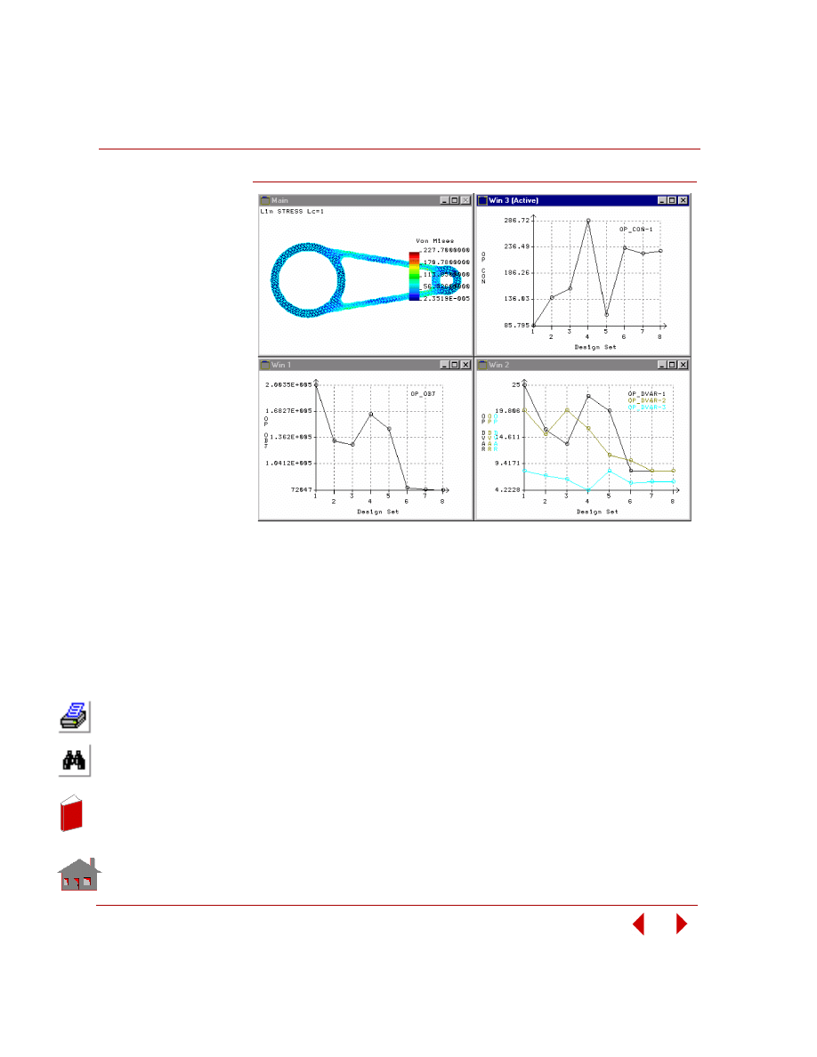
Chapter 3 Procedures and Examples
3-36
COSMOSM Advanced Modules
Figure
3-8. Final Stress Distribution and Convergence Plots
In
de
x
In
de
x
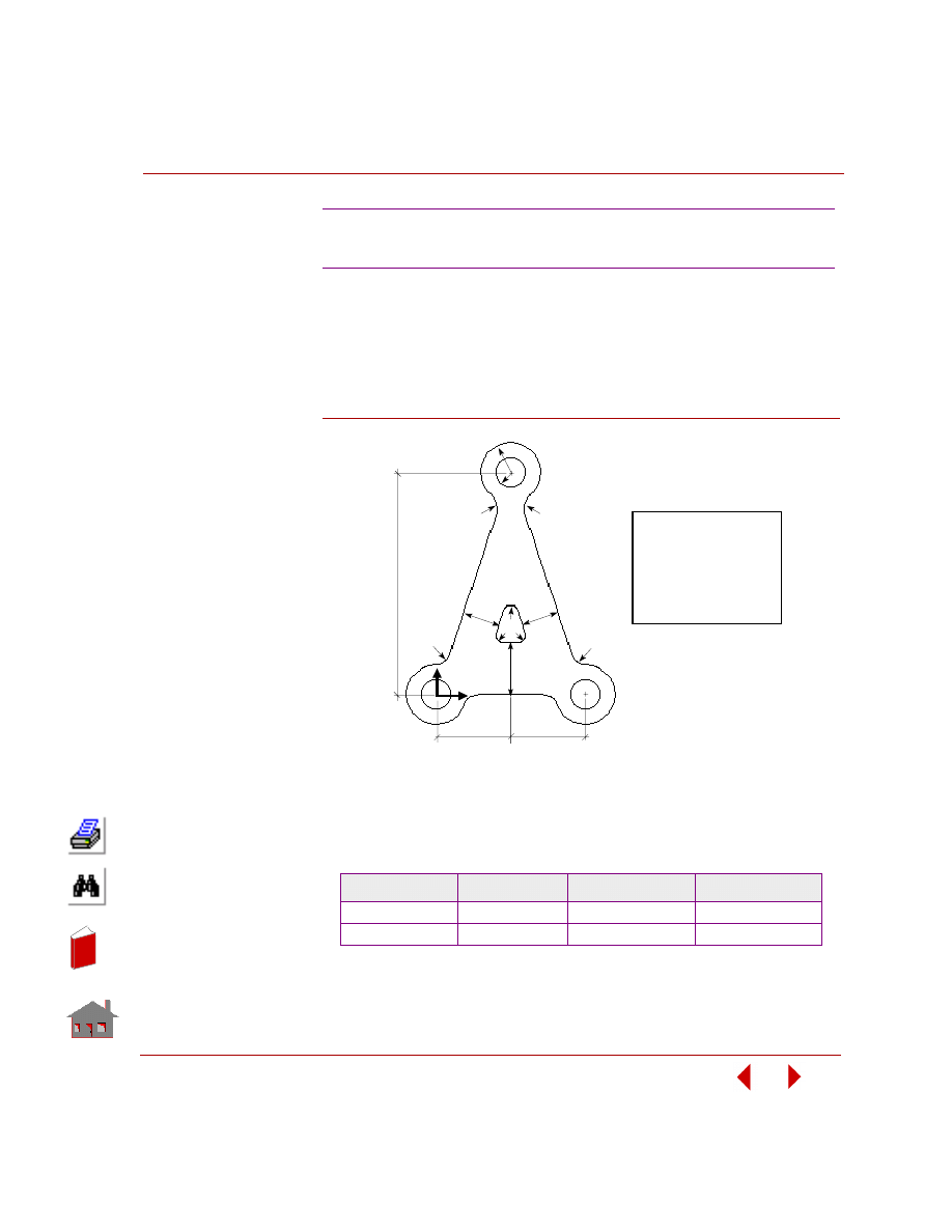
COSMOSM Advanced Modules
3-37
Part 2 OPSTAR / Optimization
In this example, you are required to find the size and location of the cutout under
the first (out-of-plane) mode of free vibration. The bracket thickness is 0.3 cm,
modulus of elasticity is 2 x 10
7
N/cm
2
, and Poisson’s ratio is 0.3. The material mass
density is 0.0075 Kg/cm
3
.
The following figure shows the initial geometry of the
bracket.
Figure
3-9. Initial Geometry of the Control Arm Bracket
The design variables for this problem as seen from the above figure are designated
as T1 and T2. Since their value will change with each sensitivity run, they will be
defined as parameters using the
PARASSIGN
(Control > PARAMETER >
Assign
Parameter
) command. The initial values and bounds for the design variables are as
shown below:
Sensitivity Study of a Control Arm
Bracket in Frequency
Design Variable
Initial Value
Lower Bound
Upper Bound
T1
2.5
0.5
2.5
T2
3.5
1.5
3.5
15.
0
1.5
1.0
Y
X
r = 1.0
r =
1.5
1.0
t
1
t
1
t
2
5.0
5.0
0.5
= 0.3 cm
= 2 x 10 N/cm
= 0.30
= 0.0075 Kg/cm
7
2
Thickness
E
Note: All dimensions in centimeters.
2
ρ
ν
S
S
S
S
S h
h
h
h
h e
e
e
e
el
l
l
l
ll
l
l
l
l3
3
3
3
3
In
de
x
In
de
x

Chapter 3 Procedures and Examples
3-38
COSMOSM Advanced Modules
Using the design variables as well as other geometric dimensions, you will first
build the initial geometry of the model parametrically. In the next step, the finite
element mesh of the initial geometry will be subjected to boundary conditions. The
frequency analysis is then performed as usual. After successful completion, you
need to specify the input for sensitivity study. During he sensitivity runs, the
program will automatically change the design variable values as required and
perform frequency analysis. The following steps describe all relevant procedures in
detail with illustration.
1.
To start with, set the working plane and the view, and initialize the design
variables T1 and T2 by executing the following commands:
Geo Panel:
Geometry > GRID >
Plane (PLANE)
PLANE;
Use the VIEW icon
VIEW;
Geo Panel:
Control > PARAMETER >
Assign Parameter (PARASSIGN)
PARASSIGN,T1,REAL,2.5,
PARASSIGN,T2,REAL,3.5,
2.
Establish the following keypoints for use in geometry creation:
Geo Panel:
Geometry > POINTS >
Define (PT)
PT,1,0,0,0,
PT,2,10,0,0,
PT,3,5,15,0,
Use Auto scaling icon
SCALE,0,
3.
Scale the view using the Auto scaling icon. Construct a triangle connecting the
three keypoints created above using the
CRLINE
(Geometry > CURVES >
Line
with 2 Pts
) command as shown below
ACTNUM
(Control > ACTIVATE >
Entity Label
) command is used to activate labels of curves):
Geo Panel:
Control > ACTIVATE >
Entity Label (ACTNUM)
ACTNUM,CR,1;
Geo Panel:
Geometry > CURVES >
Line with 2 Pts (CRLINE)
CRLINE,1,1,3,
CRLINE,2,1,2,
CRLINE,3,2,3,
In
de
x
In
de
x

COSMOSM Advanced Modules
3-39
Part 2 OPSTAR / Optimization
4.
Next, we will generate a line parallel to the base of the triangle which aligns
along the X-axis of the default Cartesian coordinate system (label 0). The
CRGEN
(Geometry > CURVES > GENERATION MENU >
Generate
)
command will be used with a Y-axis offset of T2 as illustrated below. If you
activate the SNP and PIC icons, you can select entities from the screen using the
left button of the mouse. Note that you can still use the keyboard.
Geo Panel:
Geometry > CURVES > GENERATION MENU >
Generate
(CRGEN)
Generation number [1] >
Pick/Input Beginning Curve >
2
Pick/Input Ending Curve >
2
Increment >
1
Generation flag >
Translation
X-Displacement >
0.0
Y-Displacement >
T2
Z-Displacement >
0.0
5.
In order to create lines parallel to the inclined sides of the triangle, you need to
make use of the local coordinate systems. First, define a local Cartesian
coordinate system (label 3) with its X-axis aligned with the left inclined side and
repeat the
CRGEN
(Geometry > CURVES > GENERATION MENU >
Generate
) command as shown below:
Geo Panel:
Geometry > COORD SYS >
By 3 Points (CSYS)
CSYS,3,0,3,1,2,
Geo Panel:
Geometry > CURVES > GENERATION MENU >
Generate
(CRGEN)
CRGEN,1,1,1,1,0,0,T1,0,
Next, define another local Cartesian coordinate system (label 4) with its X-axis
aligned with the right inclined side and repeat the
CRGEN
(Geometry >
CURVES > GENERATION MENU >
Generate
) command as shown below:
Geo Panel:
Geometry > COORD SYS >
By 3 Points (CSYS)
CSYS,4,0,2,3,1,
Geo Panel:
Geometry > CURVES > GENERATION MENU >
Generate
(CRGEN)
CRGEN,1,3,3,1,0,0,T1,0,
In
de
x
In
de
x
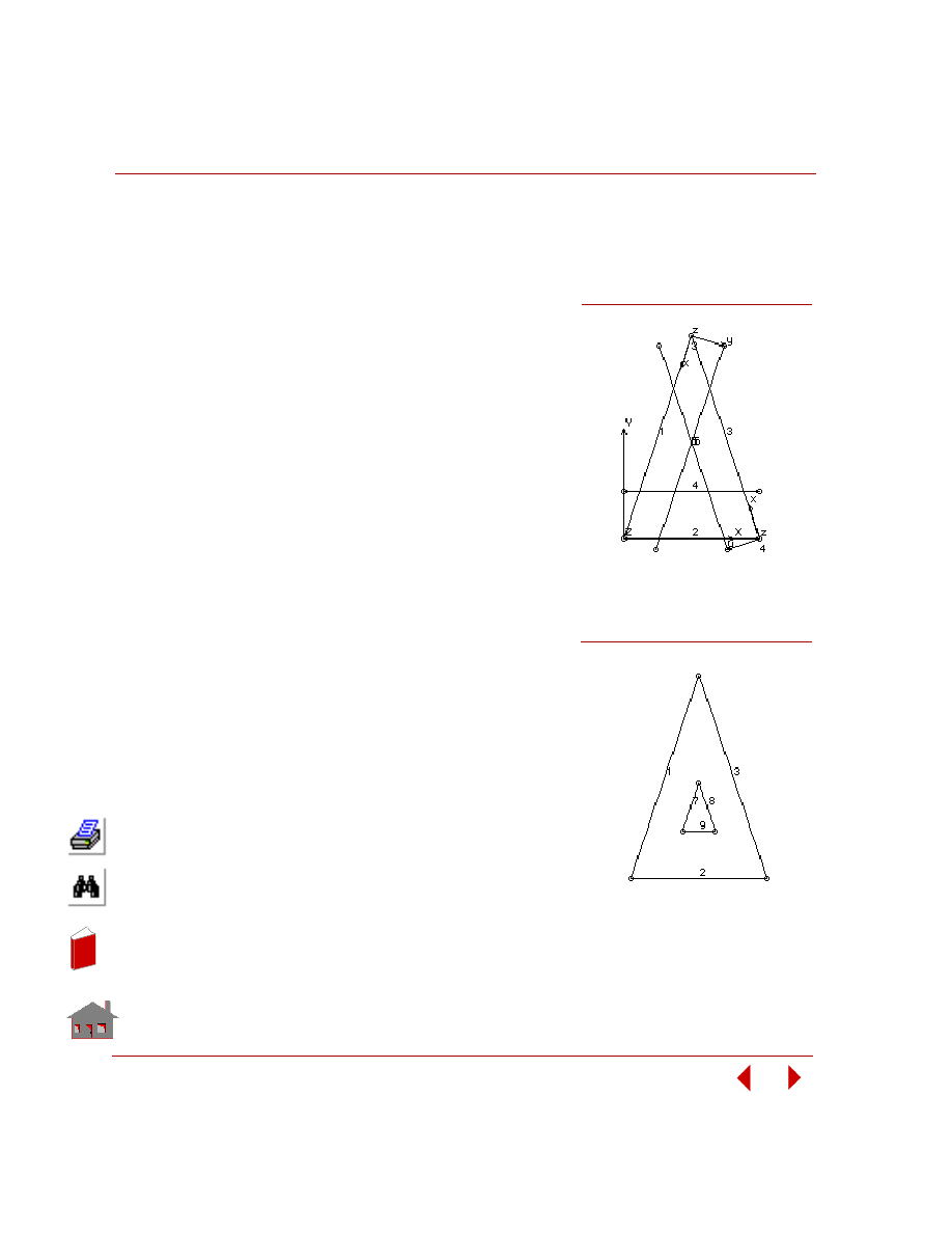
Chapter 3 Procedures and Examples
3-40
COSMOSM Advanced Modules
The following figure shows a plot of keypoints and curves generated so far, along
with the coordinate systems. In the next step, you will find the points of intersection
of curves 4 through 6 and delete the unwanted segments.
6.
Find the points of intersection of the
straight lines bounding the inner triangle
using the
CRINTCC
(Geometry >
CURVES > GENERATION MENU >
Cr/Cr Intersect
) command and delete the
unwanted segments using the
CRDEL
(Edit > DELETE >
Curves
) command:
Geo Panel:
Geometry > CURVES >
GENERATION MENU >
Cr/Cr
Intersect (CRINTCC)
CRINTCC,4,5,6,1,2,0.00005,
CRINTCC,7,8,8,1,2,0.00005,
Geo Panel:
Edit > DELETE >
Curves
CRDEL,5,6,1,
CRDEL,4,10,6,
CRDEL,11,12,1,
The geometry of the control arm is now as
shown below. Note that the corners of the
inner triangle will be rounded off using
fillets. At the corners of the outer triangle,
you will construct circles and connect them
to the rest of the geometry using procedures
similar to the above.
7.
Next, you need to create fillets at the
sharp corners created by the intersection
of straight lines with the circles. The
CRFILLET
(Geometry > CURVES >
MANIPULATION MENU >
Fillet
)
command is applied as shown below at
the sharp corners:
Figure 3-10. Construction of the
Control Arm Geometry
Figure 3-11. Construction of the
Control Arm Geometry
In
de
x
In
de
x
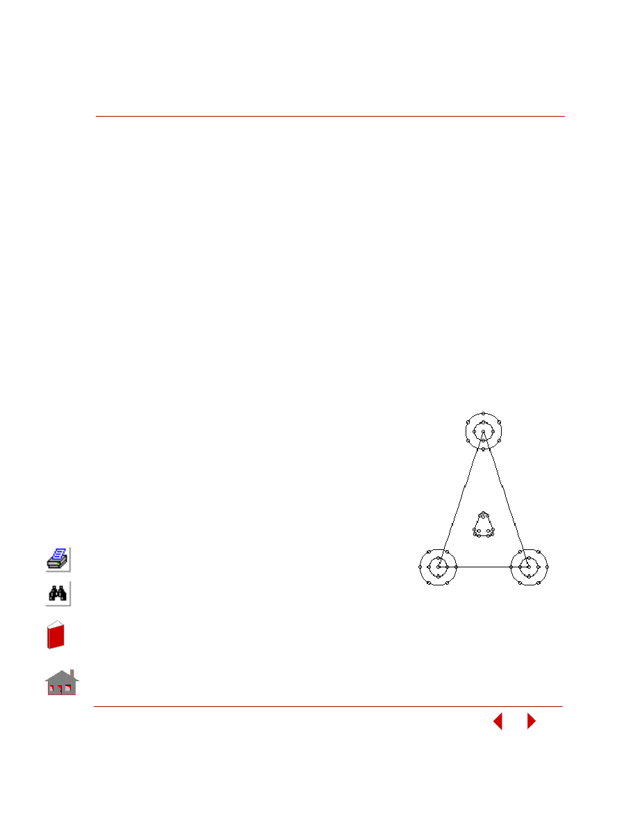
COSMOSM Advanced Modules
3-41
Part 2 OPSTAR / Optimization
Geo Panel:
Geometry > CURVES > MANIPULATION MENU >
Fillet
(CRFILLET)
CRFILLET,10,9,7,0.5,1,0,1E-006,
CRFILLET,12,7,8,0.5,1,0,1E-006,
CRFILLET,14,9,8,0.5,1,0,1E-006,
8.
Define concentric circles at the three corners as shown below:
Geo Panel:
Geometry > CURVES > CIRCLES >
Circle in Plane
(CRPCIRCLE)
CRPCIRCLE,16,1,2,1,360,4,
CRPCIRCLE,20,2,1,1,360,4,
CRPCIRCLE,24,3,20,1,360,4,
Use Auto scale icon
SCALE,0,
Geo Panel:
Geometry > CURVES > CIRCLES >
Circle in Plane
(CRPCIRCLE)
CRPCIRCLE,28,1,2,2,360,6,
CRPCIRCLE,34,2,1,2,360,6,
CRPCIRCLE,40,3,20,2,360,6,
Use Auto scale icon
SCALE,0,
The geometry of the slotted control arm you
constructed up to this stage is as shown
below. You need to find the intersection
points of the straight lines with the circles
and remove the unwanted segments.
9.
Find the points of intersection of the
straight lines with the circles using the
CRINTCC
(Geometry > CURVES >
GENERATION MENU
Cr/Cr Intersect
)
command and delete the unwanted
segments using the
CRDEL
(Edit >
DELETE >
Curves
) command:
Figure 3-12. Construction of the
Con
In
de
x
In
de
x

Chapter 3 Procedures and Examples
3-42
COSMOSM Advanced Modules
Geo Panel:
Geometry > CURVES > GENERATION MENU >
Cr/Cr Intersect (CRINTCC)
CRINTCC,1,29,45,16,2,0.00005,
Geo Panel:
Edit > DELETE >
Curves (CRDEL)
CRDEL,1,49,48,
Geo Panel:
Geometry > CURVES > GENERATION MENU >
Cr/Cr Intersect (CRINTCC)
CRINTCC,3,38,40,2,2,0.00005,
Geo Panel:
Edit > DELETE >
Curves (CRDEL)
CRDEL,3,52,49,
Geo Panel:
Geometry > CURVES > MANIPULATION MENU >
Break
Near Pt (CRPTBRK)
CRPTBRK,2,37,0,
CRPTBRK,52,43,0,
Geo Panel:
Edit > DELETE >
Curves (CRDEL)
CRDEL,2,53,51,
10.
Smoothen the sharp apices of the control arm using fillets as illustrated below:
Geo Panel:
Geometry > CURVES > MANIPULATION MENU >
Fillet
(CRFILLET)
CRFILLET,53,33,52,1.0,1,0,1E-006,
CRFILLET,54,34,52,1.0,1,0,1E-006,
CRFILLET,55,38,51,1.0,1,0,1E-006,
CRFILLET,56,46,48,1.0,1,0,1E-006,
CRFILLET,57,50,51,1.5,1,0,1E-006,
CRFILLET,58,45,48,1.5,1,0,1E-006,
11.
Delete the remaining unwanted segments as illustrated below:
Geo Panel:
Edit > DELETE >
Curves (CRDEL)
CRDEL,28,29,1,
CRDEL,39,49,10,
CRDEL,40,47,7,
With the steps executed so far, the initial geometry of the control arm is now fully
constructed. The following figure shows a view of the initial geometry. You can
next proceed to generate the finite element model.
In
de
x
In
de
x
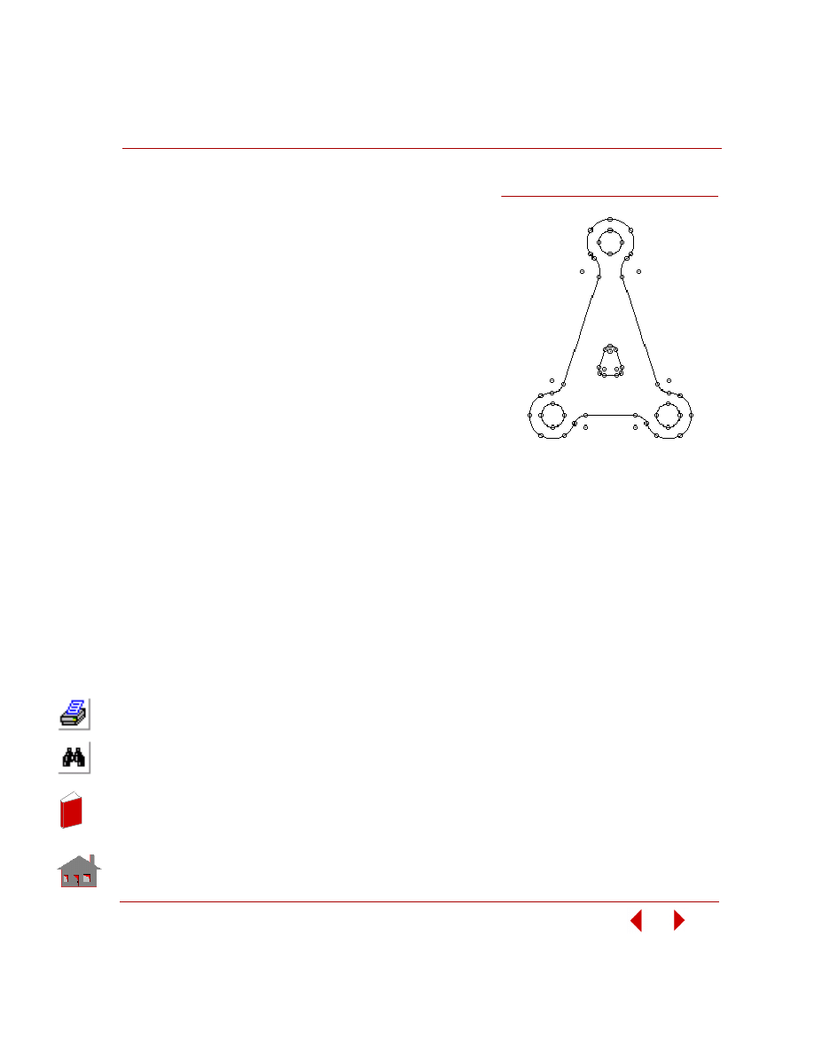
COSMOSM Advanced Modules
3-43
Part 2 OPSTAR / Optimization
12.
In order to prepare the initial
geometry for meshing, execute the
CT
(Geometry > CONTOURS >
Define
) and
RG
(Geometry >
CONTOURS >
Regions
) commands
as illustrated below:
Geo Panel:
Geometry >
CONTOURS >
Define (CT)
CT,1,0,1,1,51,0,
CT,2,0,1,1,8,0,
CT,3,0,1,1,22,0,
CT,4,0,1,1,16,0,
CT,5,0,1,1,25,0,
Geo Panel:
Geometry >
REGIONS >
Regions (RG)
RG,1,5,1,2,3,4,5,0,
13.
You will be using triangular 3-node shell elements with an average element size
of 1 units. The control arm will be held in place at the two bottom openings
against rotations and translations in all directions (we will also be switching
back to the default Cartesian global coordinate system at this stage):
Geo Panel:
Control > ACTIVATE >
Set Entity (ACTSET)
ACTSET,CS,0,
Geo Panel:
Propsets >
Element Group (EGROUP)
EGROUP,1,SHELL3,0,0,0,0,0,0,0,
Geo Panel:
Propsets >
Real Constant (RCONST)
RCONST,1,1,1,6,0.3,0,0,0,0,0,
Geo Panel:
Propsets >
Material Property (MPROP)
MPROP,1,EX,20.E6,DENS,0.0075,
Geo Panel:
Meshing > AUTO MESH >
Regions (MA_RG)
MA_RG,1,1,1,0,1,
Geo Panel:
LoadsBC > STRUCTURAL > DISPLACEMENT >
Define Contours (DCT)
DCT,3,ALL,0,4,1,
Figure 3-13. Completed Initial Geometry
of the Control Arm
In
de
x
In
de
x
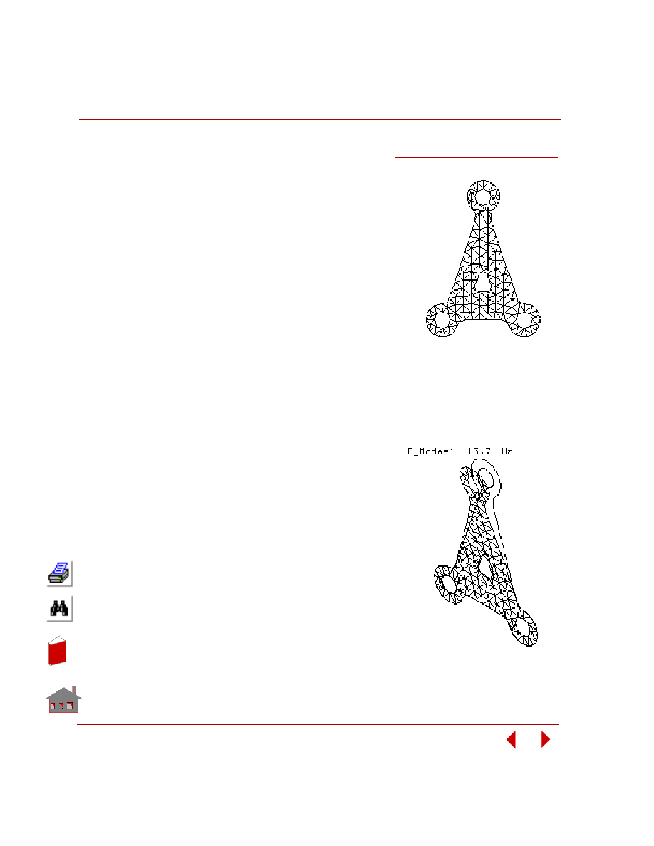
Chapter 3 Procedures and Examples
3-44
COSMOSM Advanced Modules
The following figure shows the completed
finite element mesh of the initial design.
You need to next execute the analysis to
compute the first out-of-plane free vibration
mode.
14.
Before starting the sensitivity study, you
need to run the analysis once to make
sure that you did not make any errors in
modeling or in the required features of
analysis. Execute the
R_FREQUENCY
(Analysis > FREQUENCY/
BUCKLING >
Run Frequency
)
command and use the default options
from the
A_FREQUENCY
(Analysis >
FREQUENCY/BUCKLING >
Frequency Options
) command which
include the computation of the first mode of vibration using the subspace
iteration algorithm. Note that it is possible to study the sensitivity of the model’s
frequency of different modes.
15.
It is a good practice to postprocess
the results from the preliminary
design before starting the sensitivity
study so that you can eliminate any
modeling errors by inspecting the
results. The figure below was
obtained using the
DEFPLOT
(Results > PLOT >
Deformed
Shape
) command illustrated as
follows:
Use Viewing icon to set isometric
view (XYZ)
Geo Panel:
Results > PLOT >
Deformed Shape (DEFPLOT)
Mode shape number >
1
Figure 3-14. Finite Element Mesh
of the Initial Design
Figure 3-15. Deformed Shape Plot of the
Initial Design (First Mode)
In
de
x
In
de
x

COSMOSM Advanced Modules
3-45
Part 2 OPSTAR / Optimization
16.
With the successful completion of the initial model, you can now proceed to
define the sensitivity data. As required, you will define frequency as the
response quantity:
Geo Panel:
Analysis> OPTIMIZE/SENSITIVITY> RESPONSE
QUANTITY>
Define (SN_RESPDEF)
Response set number >
1
Type >
Freq
Mode shape number >
1
Define the design variables. There are two design variables (T1 and T2) for this
problem. Each of the design variable needs to be defined separately using the
DVARDEF
(Analysis > OPTIMIZE/SENSITIVITY > DESIGN VARIABLES >
Define
) command. You also need to specify the upper and lower bounds of the
design variable under this command.
Geo Panel:
Analysis > OPTIMIZE/SENSITIVITY > DESIGN VARIABLES
>
Define (DVARDEF)
Design variable set number >
1
Design variable type >
Shape
Design variable parametric name >
T1
Design variable lower bound >
0.5
Design variable upper bound >
2.5
Accept defaults ...
Geo Panel:
Analysis > OPTIMIZE/SENSITIVITY > DESIGN VARIABLES
>
Define (DVARDEF)
Design variable set number >
2
Design variable type >
Shape
Design variable parametric name >
T2
Design variable lower bound >
1.5
Design variable upper bound >
3.5
Accept defaults ...
Lastly, the
A_SENSITIV
(Analysis > OPTIMIZE/SENSITIVITY > SENSITIVITY
RUN >
Options
) command is used to specify the sensitivity study options and the
analysis type:
Geo Panel:
Analysis > OPTIMIZE/SENSITIVITY > SENSITIVITY RUN >
Options (A_SENSITIV)
Sensitivity type >
1 by 1
Number of increment >
5
In
de
x
In
de
x

Chapter 3 Procedures and Examples
3-46
COSMOSM Advanced Modules
Output print flag >
On
Echo option flag >
On
Restart flag >
Off
Type of analysis >
Frequency
Now, you can use
R_SENSITIV
(Analysis > OPTIMIZE/SENSITIVITY >
SENSITIVITY RUN >
Run Analysis
) command to start the sensitivity study.
After ten runs, a message “sensitivity study completed” will be displayed.
17.
Use the
ACTPOST
(Results > SET UP >
Set to Post-Proc
)
,
ACTXYPOST
Display > XY PLOTS >
Activate Post-Proc
) and
XYPLOT
(Display > XY
PLOT >
Plot Curves
) commands to view the variation of the fundamental
frequency versus the design variable values.
In
de
x
In
de
x
COSMOSM Advanced Modules
4-1
4
Numerical Aspects
Introduction
The basic features and procedures for design optimization and sensitivity were
introduced in Chapter 1 to Chapter 3. These materials are sufficient in most
situations to perform the design problems.
This chapter is intended for the users who wish to learn more about the
implementation of the optimizer in OPTSTAR. Many of the methods used in the
optimizer use numerical parameters to control the convergence, tolerance, and so
on. Default values are provided for those parameters and in most situations they are
working perfectly. Nevertheless, the users are allowed to override these constants
by using appropriate commands.
The material covered in this chapter includes: basic statements of optimization
problems, function approximation, singular value decomposition, the modified
feasible direction method, the sequential linear programming method, move limits
of design variables, constraint trimming, and convergence criteria.
In
de
x
In
de
x
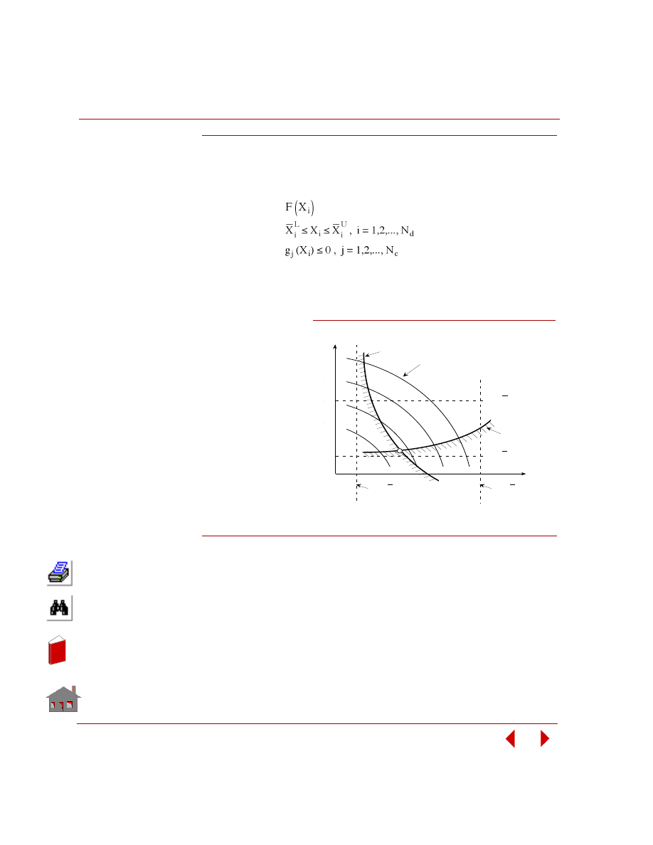
Chapter 4 Numerical Aspects
4-2
COSMOSM Advanced Modules
Basic Statements of Optimization Problems
The basic problem that we consider in OPTSTAR is the minimization of a function
subject to inequality constraints.
Figure 4-1 shows the
objective function and
constraints in the design
space with two design
variables.
It is noted that for a
maximization problem
we can always
transform it to be a
minimization one by
multiplying the
objective function by -1.
Function Approximation
The main idea of design optimization presented herein relies on finding a
mathematical relationship between the objective function or constraints and design
variables. Such a relationship is generally not known in advance.
OPTSTAR makes use of the existing response (objective function or constraints) at
a number of points in the design space to construct a polynomial approximation to
the response at other points. The optimization process is then applied to the
approximate problem represented by the polynomial approximation.
Minimize:
Objective function
Subject to:
Side constraints
Behavior constraints
where: X
i
= i
th
design variable
Figure 4-1. Objective Function and Constraints in the
Design Space with Two Design Variables
X
1
X
1
L
=
X
2
X
2
X
2
U
=
X
2
X
2
L
=
X
1
g
1
(X ,X )
g
2
F(X ,X ) = Constant
X
1
X
1
U
=
1
2
1
2
(X ,X )
1
2
In
de
x
In
de
x
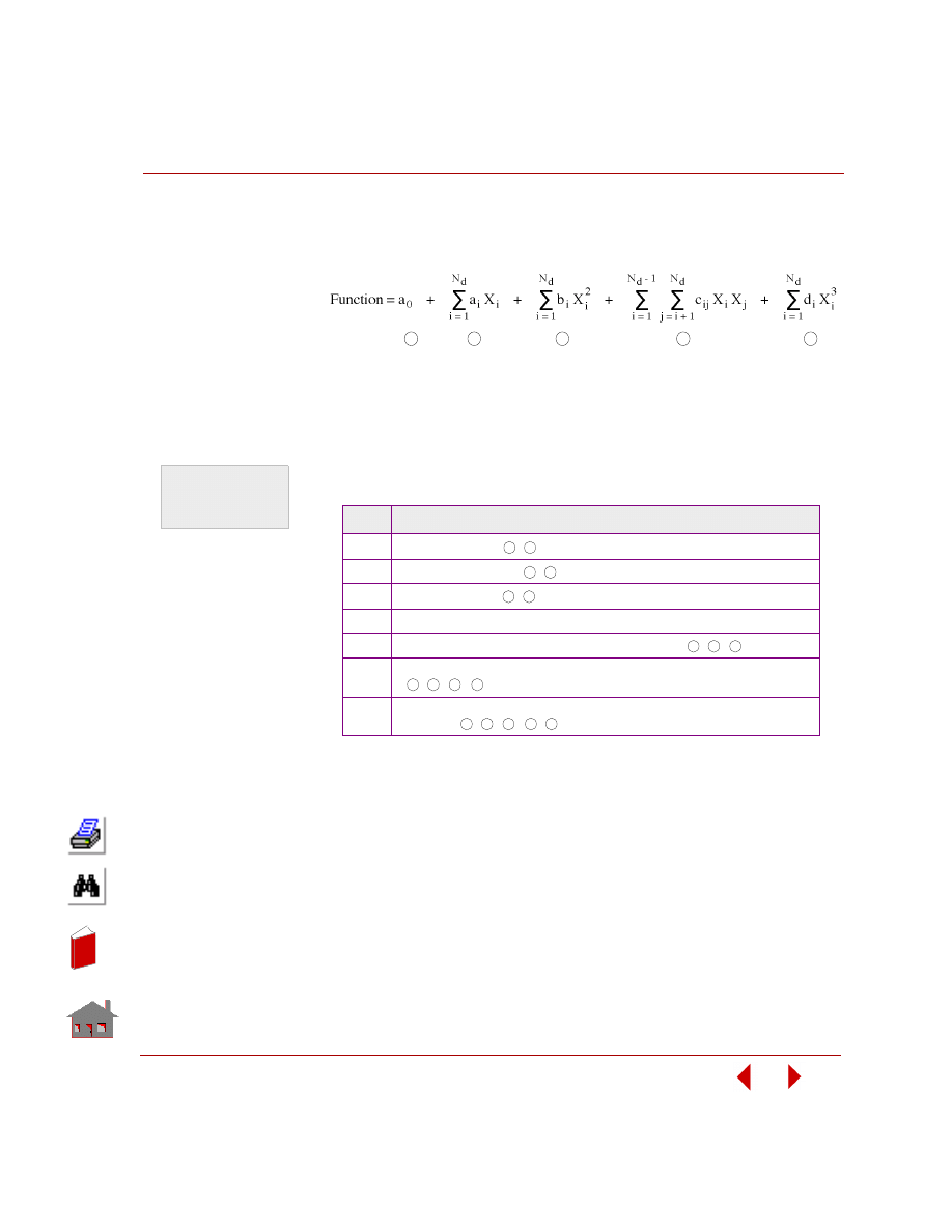
COSMOSM Advanced Modules
4-3
Part 2 OPSTAR / Optimization
Linear, quadratic, cubic, or quadratic cross-terms may be selected for the
polynomial approximation depending on the approximation type. They are as
follows:
Table 2-1. Approximation Types
For example, if we want to fit the response by the approximation type +1, we need
N
d
+2 (extra one for quality factor) design sets to start with a linear approximation.
As the optimization loop number exceeds this value, new design sets are added to
the linear approximation until it reaches 2N
d
+2. After then, a quadratic approxi-
mation is adopted. The coefficients of the polynomial function are determined by a
least squares regression.
where:
N
d
= Number of design variables
X
i
= i
th
design variable
a
i
, b
i
, c
ij
, d
i
= Coefficients to be determined
Flag
Type
-1
Only linear terms
-2
Only quadratic terms
-3
Only cubic terms
0
Automatic determination of approximation type
+1
Start with linear and add quadratic terms if needed
+2
Start with linear and add quadratic and quadratic cross terms if needed
+3
Start with linear and add quadratic, quadratic cross terms and cubic terms
if needed
1
=
2
+
3
+
4
+
5
+
OPTSTAR
(Advanced Modules
Manual, Part 2,
page 4-3)
2
)
(
1 ,
3
)
(
1 ,
5
)
(
1 ,
)
3
(
1 , 2 ,
)
3 ,
4
(
1 , 2 ,
)
3 , 4 , 5
(
1 , 2 ,
In
de
x
In
de
x
Chapter 4 Numerical Aspects
4-4
COSMOSM Advanced Modules
Singular Value Decomposition
Singular value decomposition (SVD) is used for regression analysis. It is
advantageous to use SVD because it can handle:
•
the mathematical irony that least-squares problems are both overdetermined
(number of data points greater than number of parameters) and underdetermined
(ambiguous combinations of parameters exist),
•
sets of equations that are either singular or very close to singular.
The svd_thr of the
OP_CONTROL
command sets the threshold for singular values
allowed to be non-zero. it is a ratio of the maximum singular value of the matrix.
The svd_iter of the
OP_CONTROL
command controls the maximum number of
iterations allowed to detect singular values.
The Modified Feasible Direction Method
Overall Process
After the objective function and constraints are approximated and their gradients
with respect to the design variables are calculated based on the approximation, we
are able to solve the approximate optimization problem. One of the algorithms used
in the optimizer is called the Modified Feasible Direction method (MFD). The
solving process is iterated until convergence is achieved.
It is important to distinguish the iteration inside the approximate optimization from
the loop in the overall optimization process. Figure 4-2 shows the iterative process
within each optimization loop.
In
de
x
In
de
x
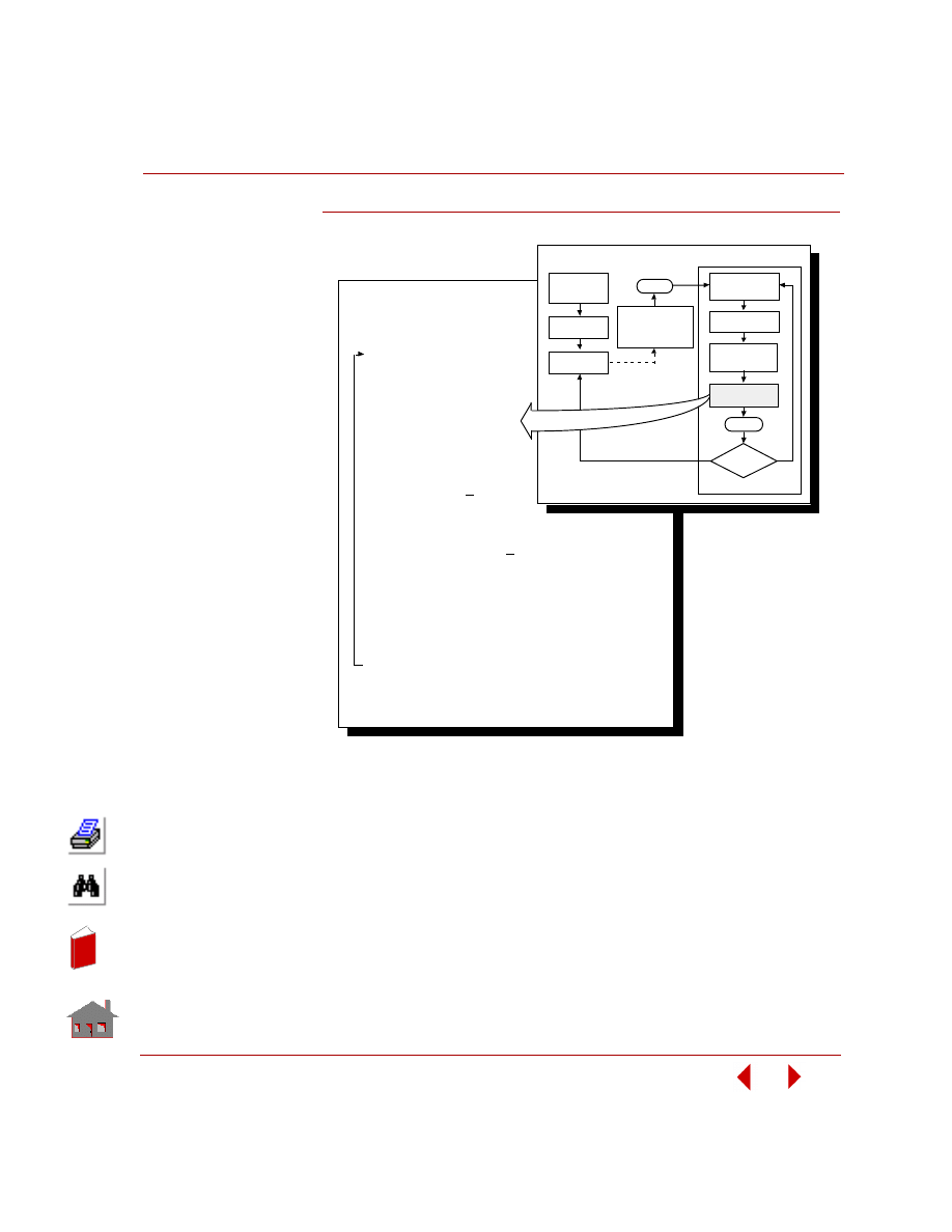
COSMOSM Advanced Modules
4-5
Part 2 OPSTAR / Optimization
Figure 4-2. The Modified Feasible Direction Algorithm
Search Direction
In order to make any further improvement in an optimization loop, a new search
direction must be found that continues to reduce the objective function but keeps
the design feasible. We seek a usable-feasible search direction, in which:
•
A usable direction is the one that reduces the objective function, and
•
A feasible direction is the one that a small move in this direction will not violate
the constraints.
q = 0, X = X
q = q + 1
Evaluate objective
function F(X ) and
behavior constraints
g (X )
≤
0
where j = 1, 2, . . ., N
Identify critical and
potentially critical
constraints, N
Calculate gradient of objective function
—F(X ) and behavior constraints
∇
g (X )
where k = 1, 2, . . ., N
Find a usable-feasible search direction S
Perform a one-dimensional search
X = X +
α
S
Check convergence. If satisfied, go to 9.
Otherwise, go to 2.
X = X
1.
2.
3.
4.
5.
6.
7.
8.
9.
M F D
q
m
m +1
q
i
j
i
c
c
i
k
i
c
q
q
q-1
q
Requirements
Achieved?
No
Yes
Update Geometry
and Mesh
(if needed) X
(m)
i
Initial
Analysis
Postprocessing
Define
m = 1
Optimization Loop
Ge ne ra l Optimiza tion
• Design Variables
• Objective Function
• Behavior Constraints
X
(1)
i
Parametric
Geometry
and Mesh
Approximate
Objective Function
and Constraints
Perform
Analysis
m = m +1
Improved
Design
X
(m+1)
i
In
de
x
In
de
x
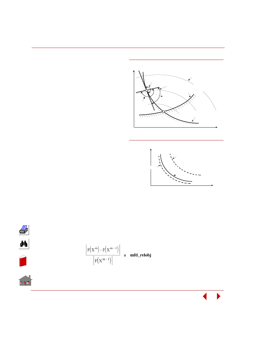
Chapter 4 Numerical Aspects
4-6
COSMOSM Advanced Modules
This situation is shown in
Figure 4-3.
To find the search
direction, active
and violated
constraints have
to be identified.
A constraint is
active if its value
lies between
mfd_viol (+ve value) and
mfd_active
(-ve value) as defined
by the command
OP_CONTROL
. A
small positive value,
mfd_viol, is allowed
before categorizing a
constraint as violated. If a
constraint is less than
mfd_active, it
is then inactive.
These conditions
are displayed in
Figure 4-4.
Convergence to the Optimum
The optimizer uses several criteria to decide when to end the iterative search process.
The criteria are described as the following.
Maximum iterations - The maximum number of iterations (search directions) is
defined by mfd_ifsrch in the command
OP_CONTROL
. It is intended to avoid
excessive computations and the default value, 100, is usually more than enough for
finding an optimum.
Changes of objective function - To measure the progress made in the successive
iterations, one of the following criteria is to be satisfied:
Figure 4-3. Usable-Feasible Search Direction
Figure 4-4. Tolerances for a Constraint in a
Two Design Variable Space
X
1
g
j
(X) = mfd_ active
X
2
g
j
( X) > 0
g
j
(X) = mfd_ viol
g
j
( X) = 0
g
j
( X) < 0
X
1
X
2
Usable
Feasible
Sector
F(X , X ) = Constant
g
2
(X , X )
= 0
g
1
Feasible
Sector
S
Usable
Sector
2
1
2
1
(X , X )
= 0
2
1
In
de
x
In
de
x
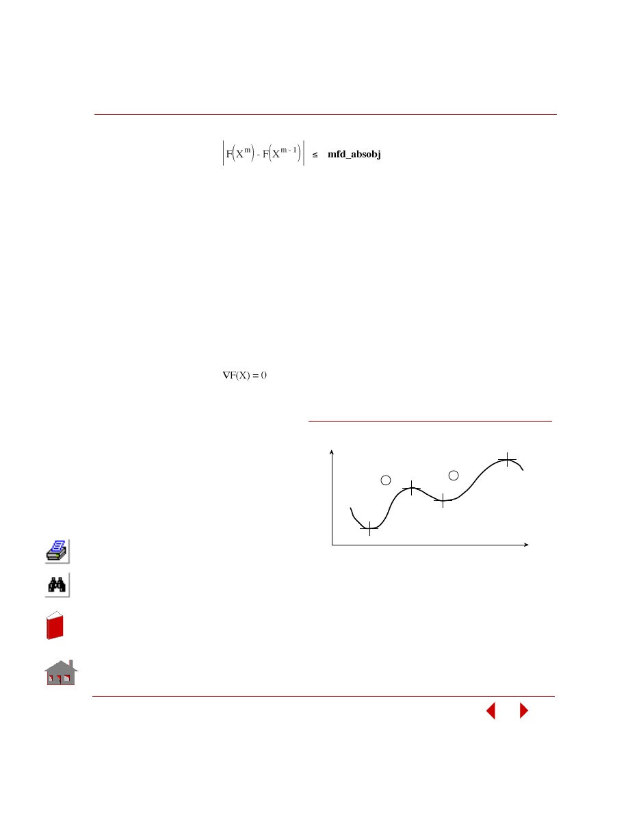
COSMOSM Advanced Modules
4-7
Part 2 OPSTAR / Optimization
or
where mfd_relobj and mdf_absobj are the specified tolerances defined in the
command
OP_CONTROL
. The first criterion, relative change, is an indication of
convergence if the objective function is large. However, the convergence is
controlled by the second criterion, absolute change, if the objective function is
small. The number of successive iterations is defined by mfd_conv in the command
OP_CONTROL
.
Satisfaction of Kuhn-Tucker Conditions
Besides the previously mentioned criteria, the Kuhn-Tucker conditions necessary
for optimality must be satisfied.
Unconstrained problems - The conditions degenerate to the case where the
gradient of the objective function vanishes:
It is noted that this
condition is
necessary but not
sufficient for
optimality. To ensure
a function to be a
minimum, the
Hessian matrix
(second derivatives
with respect to design
variables) must be
positive-definite.
Also, the optimum is
in a sense of relative
optimum rather than global one. In general, the conditions to ensure a global
minimum can rarely be demonstrated. If a global minimum is intended, the
designers must restart the optimization process from different initial points to check
if other solutions are possible. Figure 4-5 shows the relative and global minima in
the design space.
Figure 4-5. Relative and Global Minima in the Design Space
X
F(X)
1
*
2
*
In
de
x
In
de
x
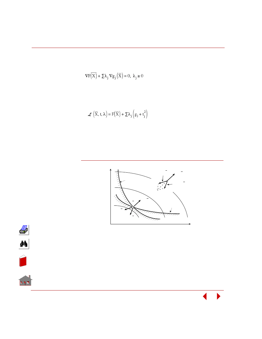
Chapter 4 Numerical Aspects
4-8
COSMOSM Advanced Modules
Constrained problems - The conditions of optimality are more complex. By using
the Lagrangian multiplier method, we define the Lagrangian function as the
following:
where t
j
is a slack variable which measures how far the j
th
constraint is from being
critical. Differentiating the Lagrangian function with respect to all variables we
obtain the Kuhn-Tucker conditions which are summarized as follows:
1.
2.
The corresponding
λ
j
is zero if a constraint is not active.
The physical interpretation of these conditions is that the sum of the gradient of the
objective function and the scalars
λ
j
times the associated gradients of the active
constraints must vectorally add to zero as shown in Figure 4-6.
Figure 4-6. Kuhn-Tucker Conditions at a Constrained Optimum
The Kuhn-Tucker conditions are also sufficient for optimality when the number of
active constraints is equal to the number of design variables. Otherwise, sufficient
conditions require the second derivatives of the objective function and constraints
(Hessian matrix) similar to the unconstrained one. If the objective function and all
of the constraints are convex, the Kuhn-Tucker conditions are also sufficient for
global optimality.
(X)
g (X)
∆
2
X
2
X
1
g
2
(X) = 0
g (X)
∆
F (X)
∆
g
1
(X) = 0
F (X)
∆
λ
g (X)
∆
1
1
λ
g (X)
∆
2
2
1
In
de
x
In
de
x
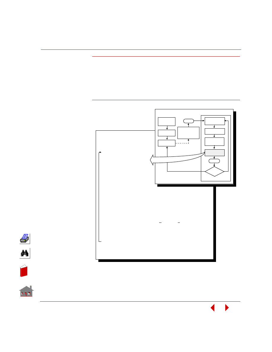
COSMOSM Advanced Modules
4-9
Part 2 OPSTAR / Optimization
The Sequential Linear Programming Method
In OPTSTAR, the other algorithm for solving the approximate optimization
problem is called the Sequential Linear Programming method (SLP). The iterative
process within each optimization loop is shown in Figure 4-7. In Figure 4-8, linear
approximations to the objective function and constraints are displayed.
Figure 4-7. The Sequential Linear Programming Method
p = 0, X = X
p = p + 1
Linearize the problem
at X by creating a
first order Taylor
Series expansion of the
objective function and
retained constraints:
F(X) = F(X ) +
∇
F(X ) (X - X )
g (X) = g (X ) +
∇
g (X ) (X - X )
Use this approximation of optimization instead of the
original nonlinear functions:
Minimize: F(X)
Subject to: g (X)
≤
0 and X
≤
X
≤
X
Find an improved design X (using the MFD algorithm)
Check feasibility and convergence. If both of them are
satisfied, go to 7. Otherwise, go to step 2.
X = X
1.
2.
3.
4.
5.
6.
7.
SLP
p
m
m +1
p
p-1
j
p-1
p-1
p-1
j
p-1
p-1
j
p-1
p
L
i
j
U
i
Requirements
Achieved?
No
Yes
Update Geometry
and Mesh
(if needed) X
(m)
i
Initial
Analysis
Postprocessing
Define
m = 1
Optimization Loop
Ge ne ra l Optimiza tion
• Design Variables
• Objective Function
• Behavior Constraints
X
(1)
i
Parametric
Geometry
and Mesh
Approximate
Objective Function
and Constraints
Improved
Design
X
(m+1)
i
Perform
Analysis
m = m +1
i
In
de
x
In
de
x
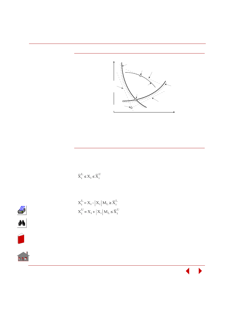
Chapter 4 Numerical Aspects
4-10
COSMOSM Advanced Modules
Figure 4-8. Linear Approximation to Objective Function and Constraints
The flag slp_iter controls the maximum number of iterations (repeated
linearization process) and slp_conv controls the number of successive iterations for
convergence check. Both flags are specified in the command
OP_CONTROL
.
Move Limits of Design Variables
During the optimization process, each design variable is bounded by its global
lower and upper limits as shown below:
Within each optimization loop, a percentage change, move limit M
L
, is temporarily
applied to the current value of design variable such that local bounds are created as:
The physical interpretation of move limits is that the optimizer creates a temporary
box around the current value of design variable as shown in Figure 4-9.
X
2
X
1
True
Oprimum
Approximate
Optimum
Linear
to g (X )
1
p
Approximation
X
p
g
1
(X)
F(X)
g
2
(X)
Linear
to g (X )
2
p
Approximation
Linear
to F (X )
p
Approximation
In
de
x
In
de
x
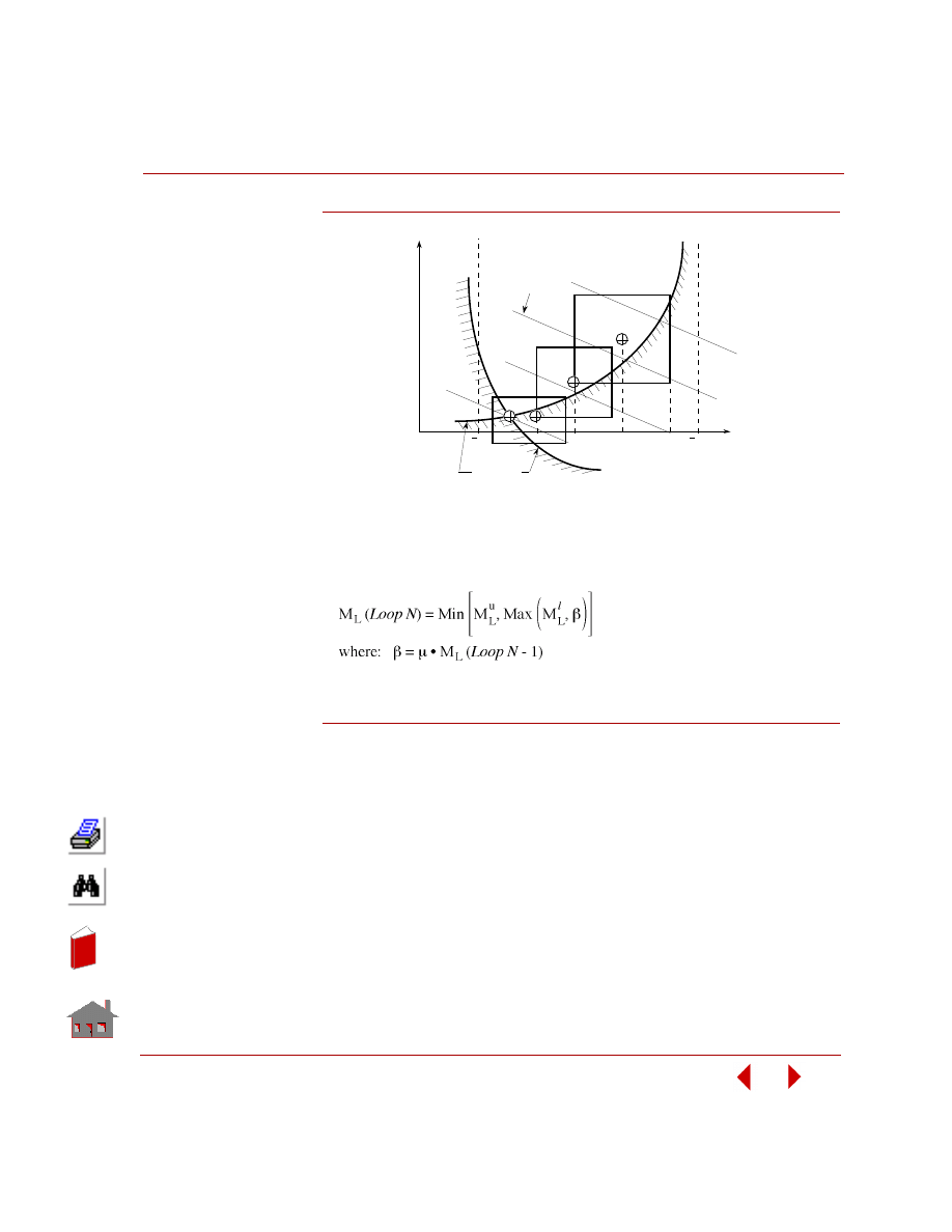
COSMOSM Advanced Modules
4-11
Part 2 OPSTAR / Optimization
Figure 4-9. Move Limits of Two Design Variables
The command
OP_DVMOVE
controls the initial move limit, its lower and upper
bounds, M
l
L
and M
u
L
, and multiplier,
µ. With these parameters, the move limit for
a subsequent optimization loop is computed by the following formula:
Constraint Trimming
Most structural optimization problems contain more constraints than what are
necessary to adequately guide the design. The constraints are filtered such that only
violated and potentially critical ones are considered in the optimizer to increase the
computational efficiency.
To identify what is meant by potentially critical, a trimming (truncation) factor is
applied to the non-violated constraints by using the command
OP_CONTRIM
. If the
normalized value of a particular constraint is below the negative value of the
trimming factor, then this constraint is temporarily deleted from the critical list. It is
Behavior
Constraint
Objective
Function
X
L
1
X
1
X
U
1
X
U
1
X
1
X
L
1
X
2
In
de
x
In
de
x
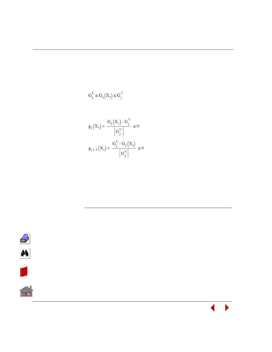
Chapter 4 Numerical Aspects
4-12
COSMOSM Advanced Modules
noted that those constraints which are temporarily deleted may become active
during the subsequent optimization loop, thus may be retained in the critical list
later.
Constraints are normalized by using their lower and upper bounds specified by the
command
OP_CONDEF
. The original constraint is bounded by:
A pair of normalized constraints with respect to upper and lower bounds are
bounded by:
This normalization provides a clear indication for the trimming. For example, a
normalized constraint with a value +0.4 has violated its bound by 40%; another
constraint with a value -0.3 is within its bound 30%. If the trimming factor is 0.2,
then the first constraint will be retained in the critical list, however the second one
will be deleted.
Convergence Criteria
Convergence or termination checks are performed at the end of each optimization
loop. The optimization process continues until either convergence or termination
occurs.
The process may be terminated before convergence in two cases:
•
The number of design sets so far exceeds the maximum number of optimization
loops specified in the command
A_OPTIMIZE
,
•
If the initial design is infeasible and the allowed number of consecutive
infeasible designs has been exceeded.
In
de
x
In
de
x
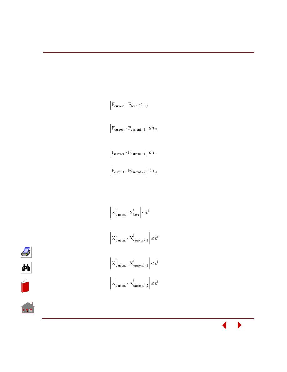
COSMOSM Advanced Modules
4-13
Part 2 OPSTAR / Optimization
The optimization problem is considered converged if all of the following conditions
are satisfied:
•
The current design is feasible,
•
Changes in the objective function F:
- The difference between the current value and the best design so far is less than
the tolerance
τF specified in the command
OP_OBJDEF
,
- The difference between the current value and the previous design is less than
the tolerance,
- (Optional) The differences between the current value and two previous designs
are less than the tolerance,
and
•
Changes in the design variables X
i
:
- The difference between the current value of each design variable and the best
design so far is less than the respective tolerance
τ
i
specified in the command
DVARDEF
,
- The difference between the current value of each design variable and the
previous design is less than the respective tolerance,
- (Optional) The differences between the current value of each design variable
and two previous designs are less than the respective tolerance,
and
In
de
x
In
de
x
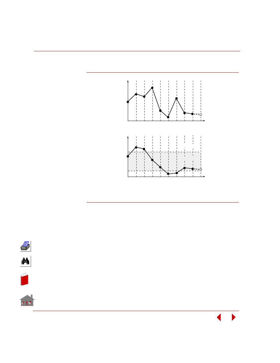
Chapter 4 Numerical Aspects
4-14
COSMOSM Advanced Modules
Figure 4-10 shows the convergence plots.
Figure 4-10. Convergence Plots
References
1.
R. T. Haftka and Z. Gürdal “Elements of Structural Optimization,” Third
Edition, Kluwer Academic Publishers, 1992.
2.
W. H. Press, B. P. Flannery, S. A. Teukolsky and W. T. Vetterling, “Numerical
Recipes,” Cambridge University Press, 1986.
3.
G. N. Vanderplaats, “Numerical Optimization techniques for Engineering
Design with Applications,” McGraw Hill, Inc., 1984.
Objective
Function
(F)
Design
Set
1
2
3
4
5
6
7
8
9
10
Constraint
Value
Design
Set
1
2
3
4
5
6
7
8
9
10
Infeasible
F easible
Infeasible
be st
F
In
de
x
In
de
x

COSMOSM Advanced Modules
5-1
5
Additional Problems
Introduction
This chapter presents additional examples for performing shape and sizing
optimization and sensitivity in COSMOSM. The input files for these problems
are available in the “...\Vprobs\Optimization” folder. Where “...” denotes the
COSMOSM directory. The prefix alphabets for the shape optimization problems
are OPS, whereas for sizing, they are OPZ. The prefix alphabets for the shape
sensitivity problems are SNS, whereas for sizing, they are SNZ. Static stress
analysis is denoted by letters ST, natural frequency analysis by FQ, buckling
analysis by BK, heat transfer analysis by HT, nonlinear by the letter N, post
dynamic analysis by D, and fatigue analysis by FT. Multidisciplinary analysis
examples use a combination of the first alphabets from the above. Note that post
dynamic and fatigue analyses are categorized to multidisciplinary since they cannot
run alone. For example, the problem OPSST5 discusses shape optimization
analysis of a beam under linear static stress analysis; OPZBK2 discusses minimum
weight of a cantilever subject to buckling constraints; OPSTSB1 addresses thermal,
static and buckling analysis of a fixed channel for the optimal shape. The following
tables provide a listing of shape and sizing optimization examples and sensitivity
with respect to the type of analysis. It is noted that the results may vary in a certain
range from one platform to another.
In
de
x
In
de
x

Chapter 5 Additional Problems
5-2
COSMOSM Advanced Modules
Table 3-1. Dominantly Shape Optimization Problems
Static
OPSST1
Stress analysis of a cantilever bracket
OPSST2
Stress analysis of a Steering Control Arm
OPSST3
Stress analysis of a slotted control arm
OPSST4
Stress analysis of a simply supported beam - line curves
OPSST5
Stress analysis of a simply supported beam - Bezier curves
OPSST6
Stress analysis for an engine bearing cap under multiple load cases
Natural
Frequency
OPSFQ1
Frequency analysis of a control arm bracket
Linearized
Buckling
OPSBK1
Buckling analysis of a C-shape column
Heat
Transfer
OPSHT1
Thermal analysis of a circular disk
OPSHT2
Thermal analysis of a pipe cooling system
OPSHT3
Thermal analysis of a simplified mechanical part
OPSHT4
Transient temperature - dependent heat conduction of a slab
Nonlinear
Structural
OPSN1
Nonlinear analysis of a thick-walled pipe
OPSN2
Nonlinear analysis of a rubber circular ring
Multi-
disciplinary
OPSFS1
Stress and frequency analysis of a bracket
OPSBS1
Stress and buckling analysis of a C-shape column
OPSTS1
Stress and thermal analysis of a mechanical part
OPSTSF1
Thermal, static and frequency analysis of a circular disk
OPSTSB1
Thermal, Static and buckling analysis of a fixed channel
OPSTN1
Transient thermal and nonlinear analysis of a cylinder
OPSFDS1
Harmonic response analysis of a culvert
OPSFDS2
Random vibration analysis of a lever arm
OPSFDS3
Response spectrum analysis of a trophy setting on a table
OPSTNFT1
Fatigue analysis of a nozzle under a cyclic temperature loading
OPSFDSFT1
Fatigue analysis of a curved pipe under a cyclic pressure loading
Table 3-2. Sizing Optimization Problems
Static
OPZST1
Minimum volume of a 1-bar truss subject to stress constraint
OPZST2
Minimum volume of a 1-bar truss subject to displacement constraint
OPZST3
Minimum volume of a 3-bar statically determinate truss subject to stress constraints
OPZST4
Minimum weight of a 3-bar statically indeterminate truss - multiple load cases
In
de
x
In
de
x

COSMOSM Advanced Modules
5-3
Part 2 OPSTAR / Optimization
Table 3-2. Sizing Optimization Problems (Continued)
Static
OPZST5
Minimum weight of a 4-bar statically indeterminate truss subject to stress constraints
OPZST6
Minimum displacement of a cantilever subject to weight constraint - beam elements
OPZST7
Minimum weight of a cantilever subject to stress constraint - beam elements
OPZST8
Minimum weight of a cantilever subject to stress constraint - beam elements
OPZST9
Minimum weight of a cantilever subject to displacement constraint - beam elements
OPZST10
Minimum stress of a simply supported rectangular plate subject to weight constraint -
shell elements
OPZST11
Minimum stress of a simply supported rectangular plate subject to stress constraint -
shell elements
OPZST12
Minimum stress of a simply supported rectangular plate subject to displ.t constraint -
shell elements
OPZST13
Minimum weight of a cantilever plate subject to stress constraint - quad. continuum
elements
OPZST14
Minimum volume of a plate subject to displacement constraint - triangular continuum
elements
OPZST15
Minimum volume of a plate subject to stress constraint - triangular continuum elements
OPZST16
Minimum volume of a plate subject to stress constraint - quadrilateral continuum elements
OPZST17
Minimum volume of a plate subject to stress constraint - quadrilateral continuum elements
OPZST18
Minimum weight of a simply supported rectangular plate subject to effective strain
constraint - shell elements
OPZST19
Minimum weight of a simply supported rectangular plate subject to strain energy density
constraint - shell elements
OPZST20
Minimum volume of a cantilever pipe subject to a stress constraint - pipe radius
OPZST21
Minimum volume of a cantilever pipe subject to a stress constraint - pipe thickness
Natural
Frequency
OPZFQ1
Minimum weight of a cantilever subject to frequency constraint - beam elements
OPZFQ2
Minimum weight of a cantilever subject to frequency constraint - shell elements
OPZFQ3
Minimum weight of a pipe cantilever subject to frequency constraint - pipe elements
In
de
x
In
de
x
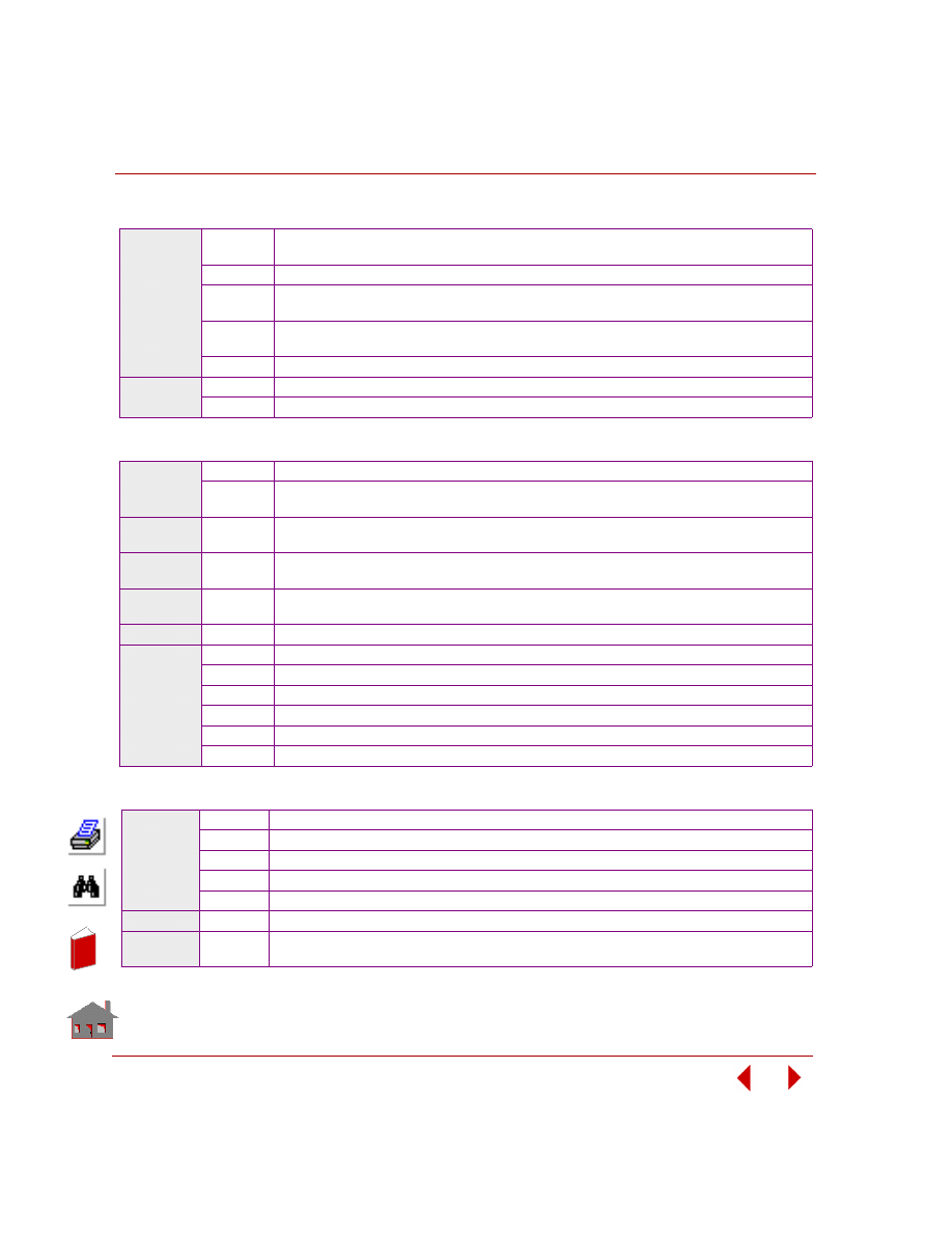
Chapter 5 Additional Problems
5-4
COSMOSM Advanced Modules
Table 3-2. Sizing Optimization Problems (continued)
Linearized
Buckling
OPZBK1
Minimum weight of a cantilever subject to buckling load factor constraint - beam elements
OPZBK2
Minimum weight of a cantilever subject to buckling constraint - shell elements
OPZBK3
Minimum weight of a cantilever plate subject to buckling constraint - quadrilateral continuum
elements
OPZBK4
Minimum weight of a pipe cantilever subject to buckling load factor - pipe elements
OPZBK5
Maximum buckling load design of a graphite-epoxy laminate
Multi-
disciplinary
OPZNB1
Snap buckling of a thin hinged cylindrical shell under a central point load
OPZFDS1
Modal time history analysis of a simply supported shell structure
Table 3-3. Dominantly Shape Sensitivity Problems
Static
SNSST1
Sensitivity study of a steering control arm in stress analysis
SNSST2
Sensitivity study of an engine bearing cap in stress analysis under multiple load cases
Natural
Frequency
SNSFQ1
Sensitivity study of a control arm bracket in frequency analysis
Linearized
Buckling
SNSBK1
Sensitivity study of a C-shape column in buckling analysis
Heat
Transfer
SNSHT1
Sensitivity study of a circular disk in heat transfer analysis
Nonlinear
SNSN1
Sensitivity study of a thick-walled pipe in nonlinear analysis
Multi-
disciplinary
SNSTSF1
Sensitivity study of a circular disk in thermal, stress and frequency analysis
SNSTSB1
Sensitivity study of C-shape column in thermal, stress and buckling analysis
SNSTN1
Sensitivity study of a cylinder in transient thermal and nonlinear analyses
SNSFDS1
Sensitivity study of a culvert in harmonic response analysis
SNSFDS2
Sensitivity study of a lever arm in random vibration analysis
SNSFDS3
Sensitivity study of a trophy in response spectrum analysis
Table 3-4. Sizing Sensitivity Problems
Static
SNZST1
Global sensitivity of a 2-bar truss: (incremented simultaneously)
SNZST2
Global sensitivity of a 2-bar truss: design variables incremented one at a time
SNZST3
Offset sensitivity of a 2-bar truss
SNZST4
Local sensitivity of a 5-bar truss
SNZST5
Sensitivity study of a graphite-epoxy laminate
Nonlinear SNZN1
Sensitivity of a rubber ring to coefficient of friction in nonlinear analysis
Multi-
disciplinary
SNZNF1A
SNZNF1B
Sensitivity study of a cantilever beam in linear, nonlinear and frequency analyses
(see page 5-116).
In
de
x
In
de
x

COSMOSM Advanced Modules
5-5
Dominantly Shape
Optimization Problems
In
de
x
In
de
x
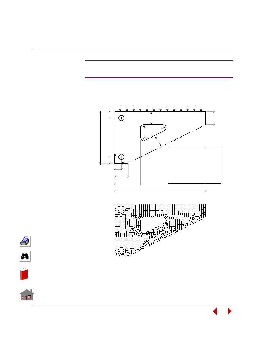
Chapter 5 Additional Problems
5-6
COSMOSM Advanced Modules
KEYWORDS:
Shape, static analysis, 8-node PLANE2D, minimum volume, and stress constraint.
OPSST1: Stress Analysis
of a Cantilever Bracket
Note: All dimensions in milimeters.
ν
100.
0
175.0
dv3
12.
5
25
dv2
dv1
Pressure
12.5
25
12.
5
Y
X
r = 5
r = 5
8 - Node P LANE 2 D
E le me nt s ( S iz e = 4 )
I nit ia l P roble m G e ome t ry
I nit ia l Finit e E le me nt Me s h
6
6
6
Thickness
Pressure
E
= 10 mm
= 5 N/mm
= 200,000 N/mm
= 0.3
2
2
In
de
x
In
de
x
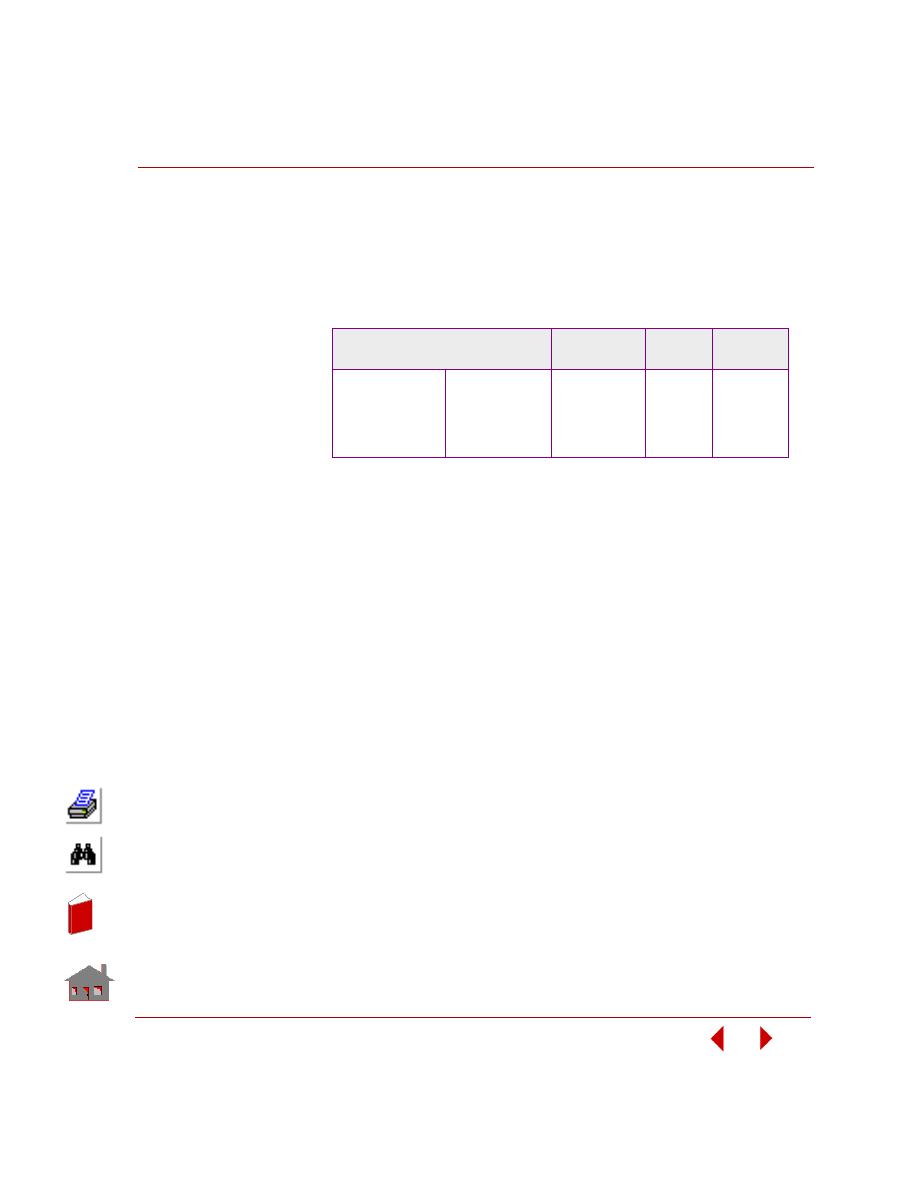
COSMOSM Advanced Modules
5-7
Part 2 OPSTAR / Optimization
PROBLEM:
Find size and location of the cutout. The bracket thickness is 10 mm, modulus of
elasticity is 200,000 N/mm
2
and Poisson's ratio is 0.3. A pressure of 5 N/mm
2
is
applied to the top edge of the bracket. The initial values and bounds of design
variables, constraints and the objective function are shown below.
SUMMARY OF RESULTS:
Optimization Parameters
Initial Value(s)
and Bounds
Final
Value(s)
Tolerance
Design Variables
DV1
DV2
DV3
10
≤
25
≤
25
10
≤
25
≤
25
20
≤
50
≤
50
19.814
10.0
20.0
2.0
2.0
2.0
Objective Function
Volume
106,794
67,600
0.05 (Ratio)
Constraints
von Mises stress
0
≤
94
≤
300
311.08
15.0
In
de
x
In
de
x
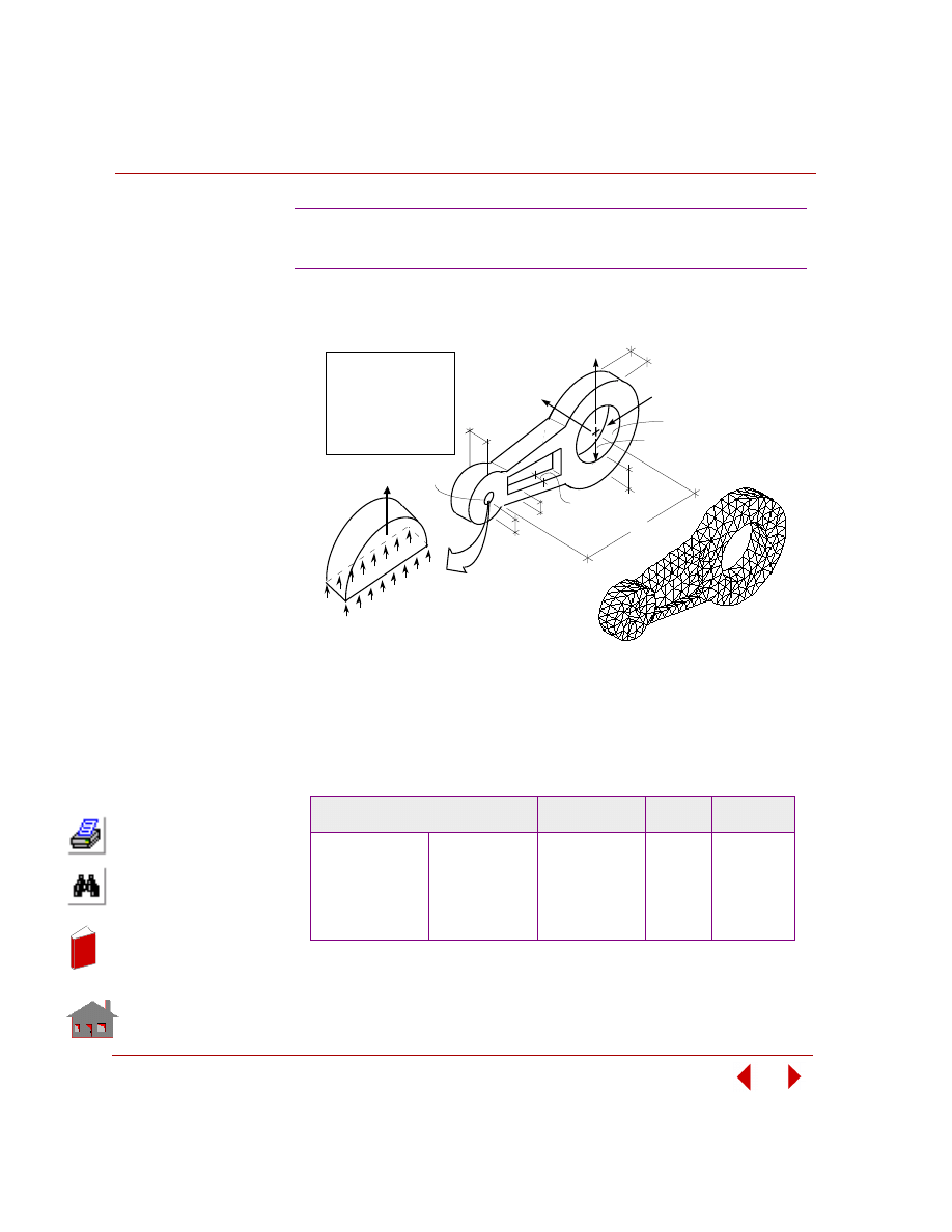
Chapter 5 Additional Problems
5-8
COSMOSM Advanced Modules
KEYWORDS:
Shape, static analysis, TETRA4, minimum volume, and stress constraint.
PROBLEM:
Find thickness of the two shafts and size and location of the cutout. The arm outer
thickness is 20 mm, modulus of elasticity is 200,000 N/mm
2
, and Poisson's ratio is
0.3. The initial values and bounds of design variables, constraints and the objective
function are shown below.
SUMMARY OF RESULTS:
OPSST2: Stress Analysis
of a Steering Control Arm
Optimization Parameters
Initial Value(s)
and Bounds
Final
Value(s)
Tolerance
Design Variables
TR1
TR2
TW
DINT
8
≤
24
≤
25
8
≤
19
≤
20
4
≤
8
≤
8
4
≤
6
≤
17
8.0
8.0
4.6981
17.00
1.0
1.0
1.0
1.0
Objective Function
Volume
218,870
76,046
0.01 (Ratio)
Constraints
von Mises stress
0
≤
105.35
≤
225
218.11
3.0
tr
tw
= 31 N/mm
Y
TE TRA4 E LE ME NTS
X
Z
20
140
20
Internal surfaces
fixed in all directions
30
tr
1
7
I nit ia l P roble m
G e ome t ry
I nit ia l Finit e
E le me nt Me s h
dint
= 2 x 10 N/mm
= 0.3
E
Note: All dimensions
in milimeters.
ν
2
2
P
y
2
Y
P
y
5
In
de
x
In
de
x
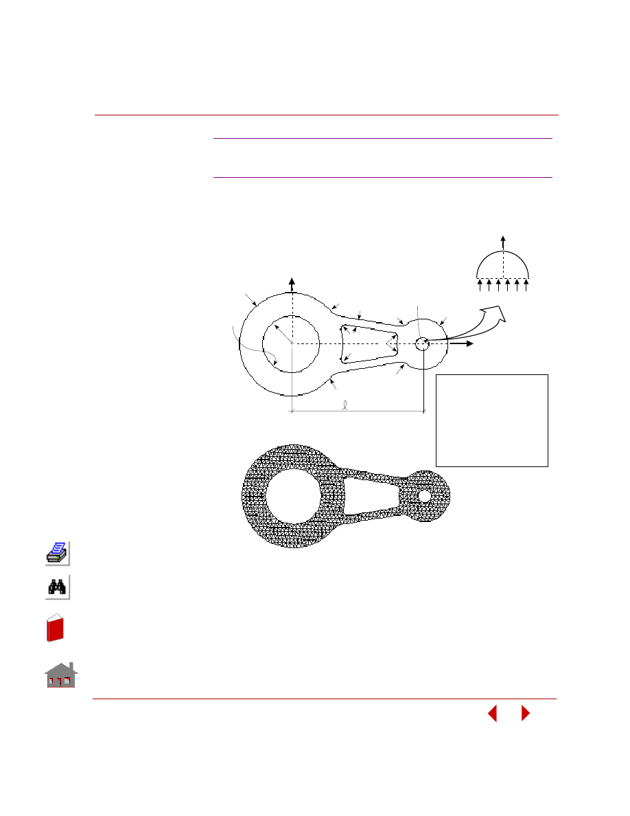
COSMOSM Advanced Modules
5-9
Part 2 OPSTAR / Optimization
KEYWORDS:
Shape, static analysis, 6-node TRIANG, minimum volume, and stress constraint.
OPSST3: Stress Analysis
of a Slotted Control Arm
I nit ia l Finit e E le me nt Me s h
5
5
5
tr
Fixed
= 140
1
20
20
10
10
r = 7
P
Y
6 - Node
Tria ngula r Me s h
= 20 mm
= 2 x 10 N/mm
2
5
= 0.3
= 4 N/mm
(Y direction)
Thickness
E
Note: All dimensions in milimeters.
ν
2
P
I nit ia l P roble m G e ome t ry
2
r = 30
1
y
Y
y
tr
2
X
t w
In
de
x
In
de
x
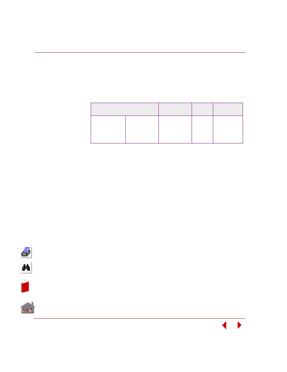
Chapter 5 Additional Problems
5-10
COSMOSM Advanced Modules
PROBLEM:
Find thickness of the two shafts and size and location of the cutout. The arm outer
thickness is 20 mm, modulus of elasticity is 200,000 N/mm
2
, and Poisson's ratio is
0.3. The initial values and bounds of design variables, constraints and the objective
function are shown below.
SUMMARY OF RESULTS:
Optimization Parameters
Initial Value(s)
and Bounds
Final
Value(s)
Tolerance
Design Variables
TR1
TR2
TW
8
≤
25
≤
25
8
≤
20
≤
20
3.5
≤
8
≤
8
8.0
8.0
5.8192
1.0
1.0
0.5
Objective Function
Volume
200,347.9
72,047.13
0.00125 (Ratio)
Constraints
von Mises stress
10
≤
90.64
≤
225
227.70
3.0
In
de
x
In
de
x
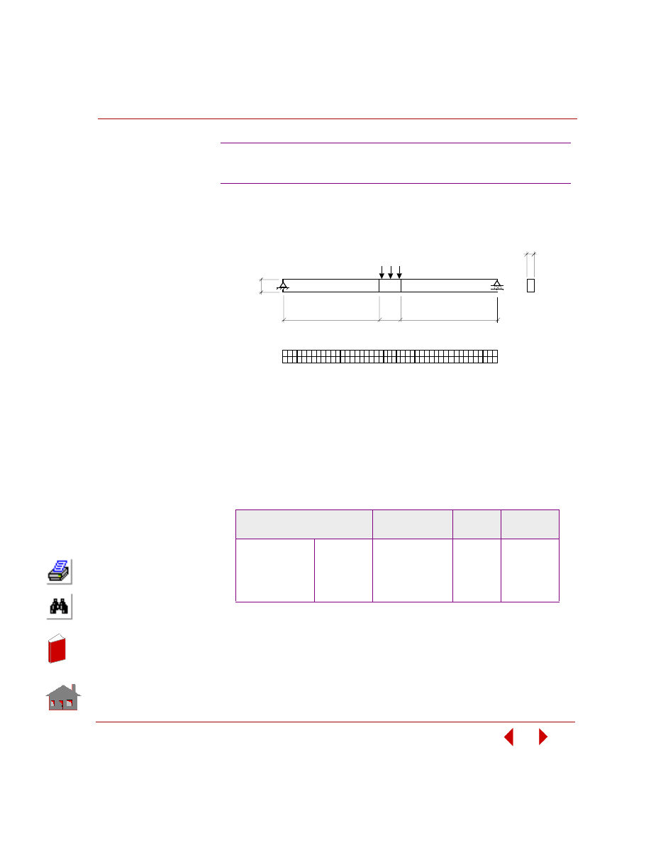
COSMOSM Advanced Modules
5-11
Part 2 OPSTAR / Optimization
KEYWORDS:
Shape, static analysis, 8-node SOLID, minimum volume, and stress constraint.
PROBLEM:
Find height of the beam at support and middle part. The beam width is 4 in, modulus
of elasticity is 1E7 psi, and Poisson's ratio is 0.3. Nodal forces of 100 lb are applied
to the middle part of the beam. The initial values and bounds of design variables,
constraints and the objective function are shown below.
SUMMARY OF RESULTS:
OPSST4: Stress Analysis of a Simply
Supported Beam – Line Curves
Optimization Parameters
Initial Value(s)
and Bounds
Final
Value(s)
Tolerance
Design Variables
D1
D2
0.2
≤
6
≤
10
0.2
≤
6
≤
10
1.4442
3.4309
0.098
0.098
Objective Function
Volume
2400
1014.8
0.03 (Ratio)
Constraints
von Mises 1
von Mises 2
1
≤
1575.6
≤
5000
1
≤
1648.2
≤
5000
4949.7
5033.3
49.99
49.99
45"
Cros s
S e c t ion
45"
10"
D
1
100 lbs/Node
D
2
4"
I nit ia l P roble m G e ome t ry
I nit ia l Finit e E le me nt Me s h
In
de
x
In
de
x
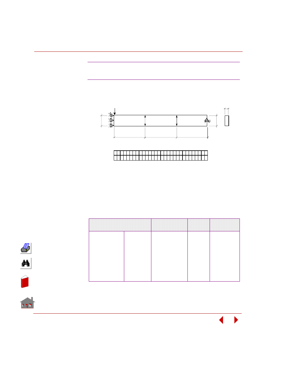
Chapter 5 Additional Problems
5-12
COSMOSM Advanced Modules
KEYWORDS:
Shape, static analysis, 8-node SOLID, minimum volume, and stress constraint.
PROBLEM:
Find heights along the beam span. The beam width is 4 in, modulus of elasticity is
1E7 psi, and Poisson's ratio is 0.3. Nodal forces of 1000 lb are applied at the mid-
section of the beam. The initial values and bounds of design variables, constraints
and the objective function are shown below.
SUMMARY OF RESULTS:
OPSST5: Stress Analysis of a Simply
Supported Beam – Bezier Curves
Optimization Parameters
Initial Value(s)
and Bounds
Final
Value(s)
Tolerance
Design Variables
D1
D2
D3
D4
0.1
≤
6
≤
10
0.1
≤
6
≤
10
0.1
≤
6
≤
10
0.1
≤
6
≤
10
4.2882
4.1135
1.8693
1.8858
0.099
0.099
0.099
0.099
Objective Function
Volume
1,440.0
729.42
0.03125 (Ratio)
Constraints
von Mises 1
von Mises 2
von Mises 3
von Mises 4
von Mises 5
1
≤
7401.2
≤
15000
1
≤
5255.1
≤
15000
1
≤
2759.7
≤
15000
1
≤
3409.7
≤
15000
1
≤
7378.1
≤
15000
15,124
14,035
15,052
2681.5
15,110
149.99
149.99
149.99
149.99
149.99
4"
20"
20"
D
1
D
2
Cros s
S e c t ion
D
3
D
4
20"
1,000 lbs/node
init ia l P roble m G e ome t ry
init ia l Finit e E le me nt Me s h
In
de
x
In
de
x
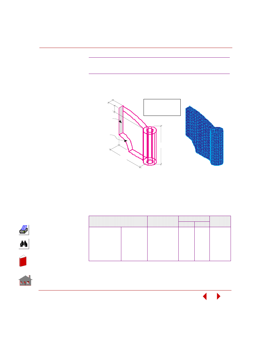
COSMOSM Advanced Modules
5-13
Part 2 OPSTAR / Optimization
KEYWORDS:
Shape, static analysis, TETRA10, multiple load cases, minimum volume, and stress
constraint.
PROBLEM:
Find size and geometric dimensions of the bearing cap. The bearing cap modulus of
elasticity is 200,000 N/mm
2
and Poisson's ratio is 0.30. A horizontal pressure (as
load case 1) and a vertical pressure (as load case 2) are applied to the internal
surfaces of the cylindrical hole. The initial values and bounds of design variables,
constraints and objective function are shown below.
SUMMARY OF RESULTS:
OPSST6: Stress Analysis of an Engine
Bearing Cap Under Multiple Load Cases
Optimization Parameters
Initial Value(s)
and Bounds
Final Value(s)
Tolerance
STAR
FFE
Design Variables
ECCENT
TWEB
HEIGHT
HUMP
50
≤
75
≤
75
6
≤
10
≤
10
40
≤
70
≤
70
1
≤
15
≤
15
50
6.6044
40
6.7424
50
6
40
9.7574
0.25
0.04
0.30
0.14
Objective Function
Volume
69,844.78
21,767
21,450
0.05 (Ratio)
Constraints
von Mises
stress
STAR: 0
≤
117.4
FFE: 113.6
≤
250
259.21
261.02
12.50
Fixed
ECCENT
Height
Initial
P roble m
Ge ome try
TWEB
Symmetry
Boundary
Conditions
HUMP
1 0 -Node Te tra Me sh
E
ν
= 2 x 10 N/mm
= 0.30
5
2
Initial Finite
E le me nt Me sh
In
de
x
In
de
x
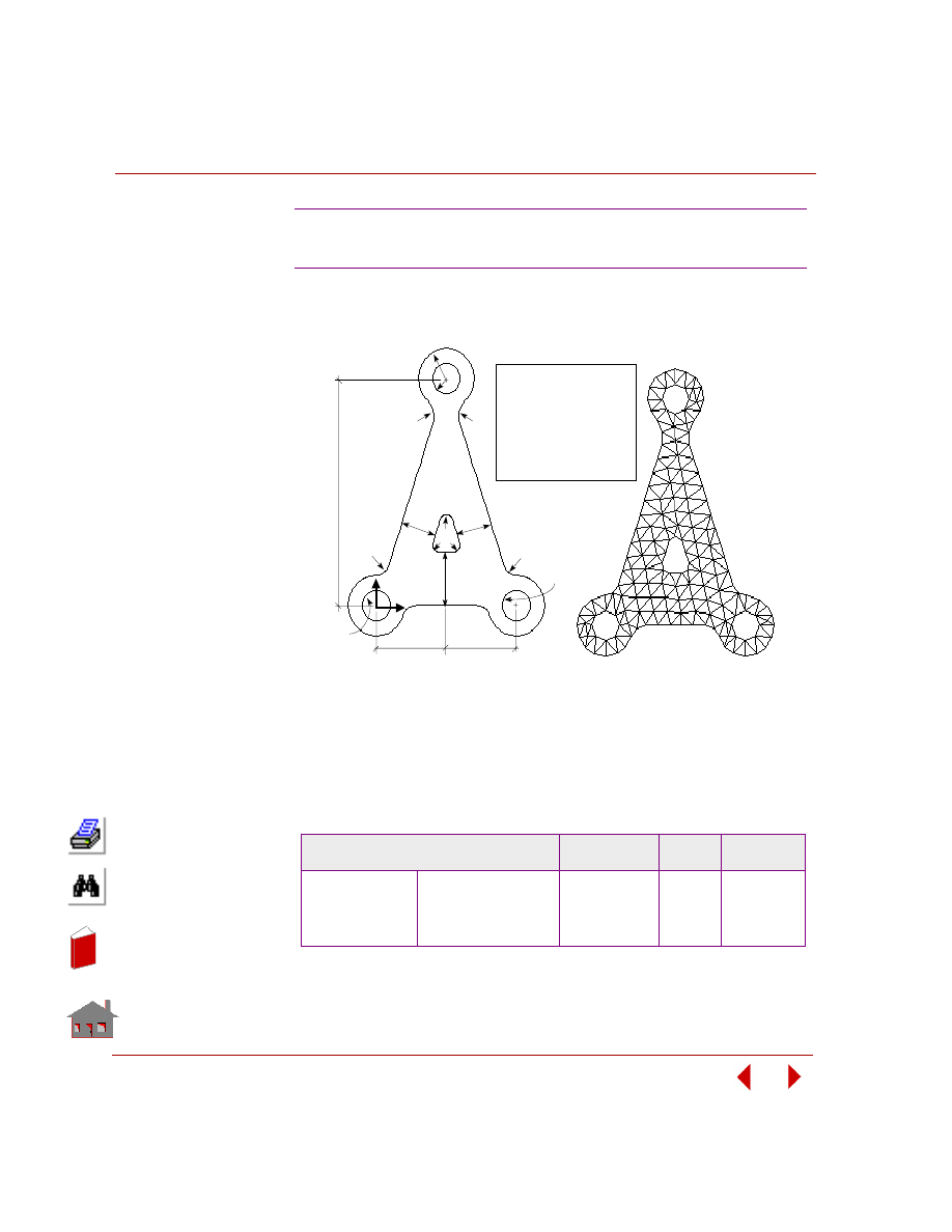
Chapter 5 Additional Problems
5-14
COSMOSM Advanced Modules
KEYWORDS:
Shape, frequency analysis, SHELL3, minimum volume, and frequency constraint.
PROBLEM:
Find size and location of the cutout. The bracket thickness is 0.3 cm, modulus of
elasticity is 2E7 N/cm
2
, and Poisson's ratio is 0.3. The material mass density is
0.0075 Kg/cm
3
. T
he initial values and bounds of design variables, constraints and the
objective function are shown below.
SUMMARY OF RESULTS:
OPSFQ1: Frequency Analysis
of a Control Arm Bracket
Optimization Parameters
Initial Value(s)
and Bounds
Final
Value(s)
Tolerance
Design Variables
T1
T2
0.5
≤
2.5
≤
2.5
1.5
≤
3.5
≤
3.5
0.6256
1.5
0.02
0.02
Objective Function
Volume
28.473
16.491
0.008 (Ratio)
Constraints
Fundamental frequency
8
≤
13.65
≤
14
7.9992
0.06
15.
0
1.5
1.0
Y
X
r = 1.0
r = 2.0
1.5
1.0
t
1
t
1
t
2
5.0
5.0
0.5
3 - Node Tria ngula r
Me s h ( S iz e = 1 )
= 0.3 cm
= 2 x 10 N/cm
= 0.30
= 0.0075 Kg/cm
7
2
Thickness
E
Note: All dimensions in centimeters.
3
ρ
ν
I nit ia l P roble m G e ome t ry
I nit ia l Finit e E le me nt Me s h
Fixed
Fixed
In
de
x
In
de
x

COSMOSM Advanced Modules
5-15
Part 2 OPSTAR / Optimization
KEYWORDS:
Shape, buckling analysis, SHELL3, minimum volume, and buckling load factor
constraint.
OPSBK1: Buckling Analysis
of a C-shape Column
I nit ia l Finit e
E le me nt Me s h
B = 20"
T
2
T
1
A = 6"
C = 3"
Fixed
T
2
T
1
T
2
T
1
h = 120"
0.18h
0.32h
0.32h
0.18h
p =
5,000 psi
(T /4)
2
Fillet
I nit ia l P roble m
G e ome t ry
= 3 in
= 0. 25 in
= A_ Steel
Element Size
Thickness
Material
S HE LL3
E
= 0.28
ν
= 3 x 10 psi
7
ρ
= 0.73 x 10 lbf sec /in
-3
2
4
In
de
x
In
de
x
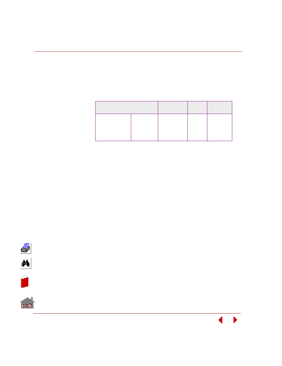
Chapter 5 Additional Problems
5-16
COSMOSM Advanced Modules
PROBLEM:
Find size of the column cutouts. The cross section thickness is 0.25 in., modulus of
elasticity is 3E7 psi, and Poisson's ratio is 0.28. A pressure of 5000 psi is applied to
the column's face. The initial values and bounds of design variables, constraints and
the objective function are shown below.
Summary of Results:
Optimization Parameters
Initial Value(s)
and Bounds
Final
Value(s)
Tolerance
Design Variables
T1
T2
1
≤
5
≤
35
1
≤
5
≤
12
35.0
11.261
0.34
0.11
Objective Function
Volume
1018.15
745.91
0.01 (Ratio)
Constraints
Buckling load
factor
1.6
≤
2.87
≤
10
1.5843
0.02
In
de
x
In
de
x
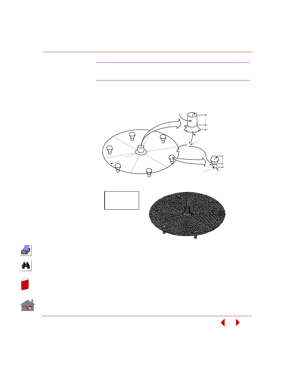
COSMOSM Advanced Modules
5-17
Part 2 OPSTAR / Optimization
KEYWORDS:
Shape, thermal analysis, SHELL3, minimum volume, and temperature constraint.
OPSHT1: Thermal Analysis
of a Circular Disk
Initial Finite E le me nt Me sh
25
10
5
= 2 mm
Thickness
3 - Node S he ll
Me s h ( S iz e = 2 )
10
5
5
5
2
Heat Flux
0.1 W/mm
Heat Flux
0.1 W/mm
2
Convection 0.0005 W/mm -
°
C
Ambient Temperature 50
°
C
2
Convection 0.0 W/mm -
°
C
Ambient Temperature 50
°
C
2
10
25
Radius
5
Initial P roble m Ge ome try
In
de
x
In
de
x

Chapter 5 Additional Problems
5-18
COSMOSM Advanced Modules
PROBLEM:
Find radius of the disk. The disk thickness is 2 mm, and conductivity is 0.57
W/mm-
°C. A convection of 0.0005 W/mm-°C with an ambient temperature of 50 °C
is applied to the entire model except for the heat sources. The heat source regions
(heat flux of 0.1 W/mm
2
) is assumed to have a convection of 0 W/mm
2
-
°C with an
ambient temperature of 50
°C. The initial values and bounds of design variables,
constraints and the objective function are shown below.
SUMMARY OF RESULTS:
Optimization Parameters
Initial Value(s)
and Bounds
Final
Value(s)
Tolerance
Design Variables
Radius
30
≤
70
≤
70
30.849
1.0
Objective Function
Volume
33,375.56
8566.86
0.0015 (Ratio)
Constraints
Temperature
50
≤
77.63
≤
140
140.15
1.0
In
de
x
In
de
x
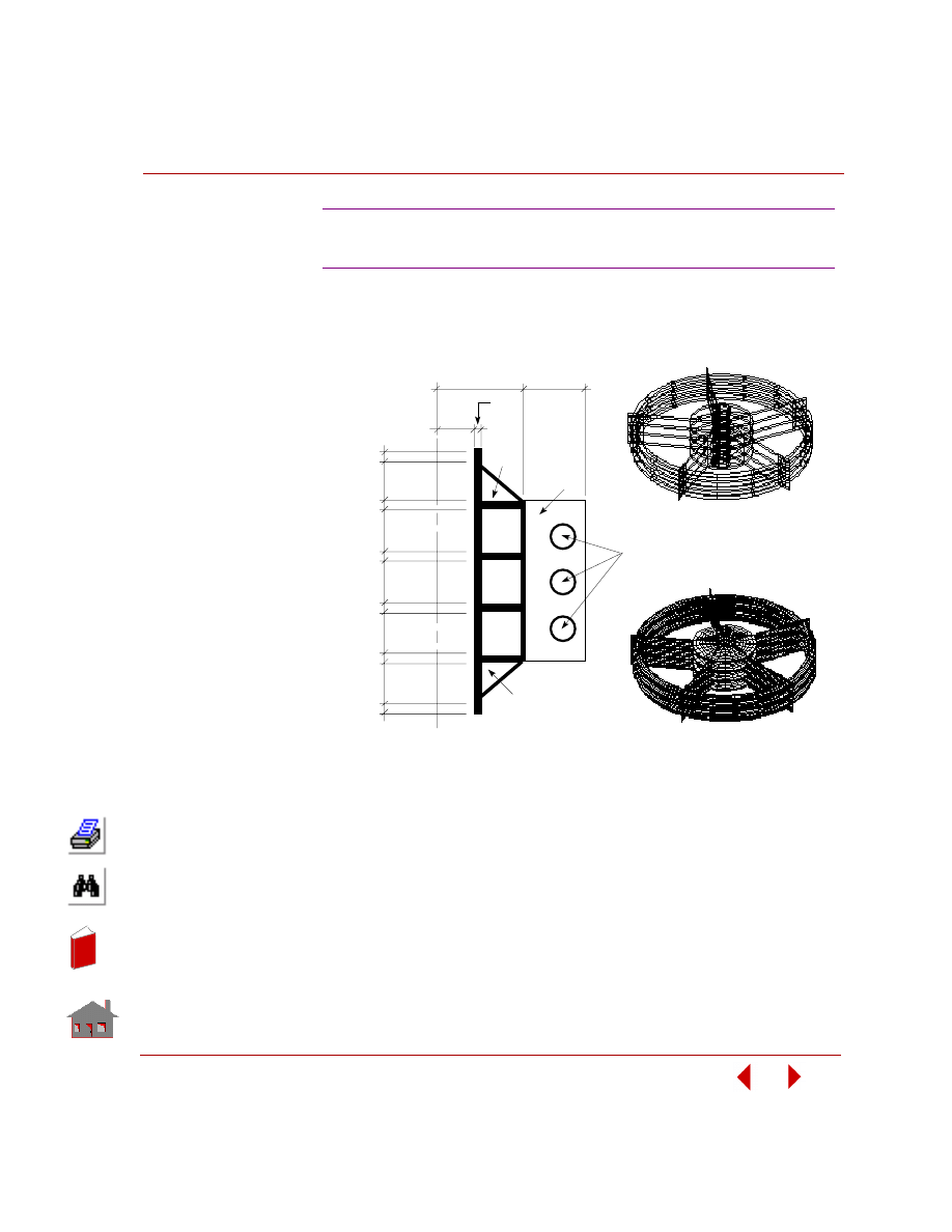
COSMOSM Advanced Modules
5-19
Part 2 OPSTAR / Optimization
KEYWORDS:
Shape, thermal analysis, 8-node SOLID, SHELL4, minimum volume, and
temperature constraint.
OPSHT2: Thermal Analysis
of a Pipe Cooling System
T
3
T
3
T
3
T
3
T
3
R4 (thickness of
pipes = 0.2 mm)
T
3
RADD
2
R = 5
T
1
T
2
T
2
T
2
T
2
H = 5
1
H = 7
2
H = 5
1
H = 7
2
H = 7
3
H = 7
3
H = 7
3
I nit ia l P roble m G e ome t ry
I nit ia l Finit e E le me nt Me s h
1
Cros s S e c t ion
R
In
de
x
In
de
x
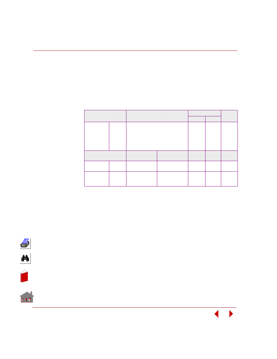
Chapter 5 Additional Problems
5-20
COSMOSM Advanced Modules
PROBLEM:
Find radii and thicknesses of plates and pipes of the cooling system. The material
conductivity is 0.57 W/mm-
°C. A convection of 0.0015 W/mm
2
-
°C with an ambient
temperature of 50
°C is applied to the entire model except for the heat source. The
heat source region (heat flux of 0.1 W/mm
2
) is assumed to have a convection of
0 W/mm
2
-
°C with an ambient temperature of 50°C The initial values and bounds of
design variables, constraints and the objective function are shown below.
SUMMARY OF RESULTS:
Optimization
Parameters
Initial Value(s) and Bounds
Final Value(s)
Toler-
ance
HSTAR
FFE
Design
Variables
R2
RADD
R4
T1
T2
T3
13
≤
25
≤
25
8
≤
50
≤
50
1
≤
3
≤
3
1
≤
2
≤
2
1
≤
2
≤
2
1
≤
2
≤
2
13.0
8.0
1.0
1.3246
1.0
1.0
13.0
8.0
1.0
1.3671
1.0
1.0
1.0
1.0
0.1
0.1
0.1
0.1
Optimization
Parameters
HSTAR
FFE
HSTAR
FFE
Toler-
ance
Objective
Function
Weight
196.436
196.436 37.0046
37.588
0.001
(Ratio)
Constraints
Temp 1
Temp 2
Temp 3
50
≤
77.33
≤
100
50
≤
76.36
≤
100
50
≤
50.55
≤
100
50
≤
77.34
≤
100
50
≤
76.36
≤
100
50
≤
50.56
≤
70
100.18
98.995
68.317
99.754
98.602
68.264
1.0
1.0
1.0
In
de
x
In
de
x
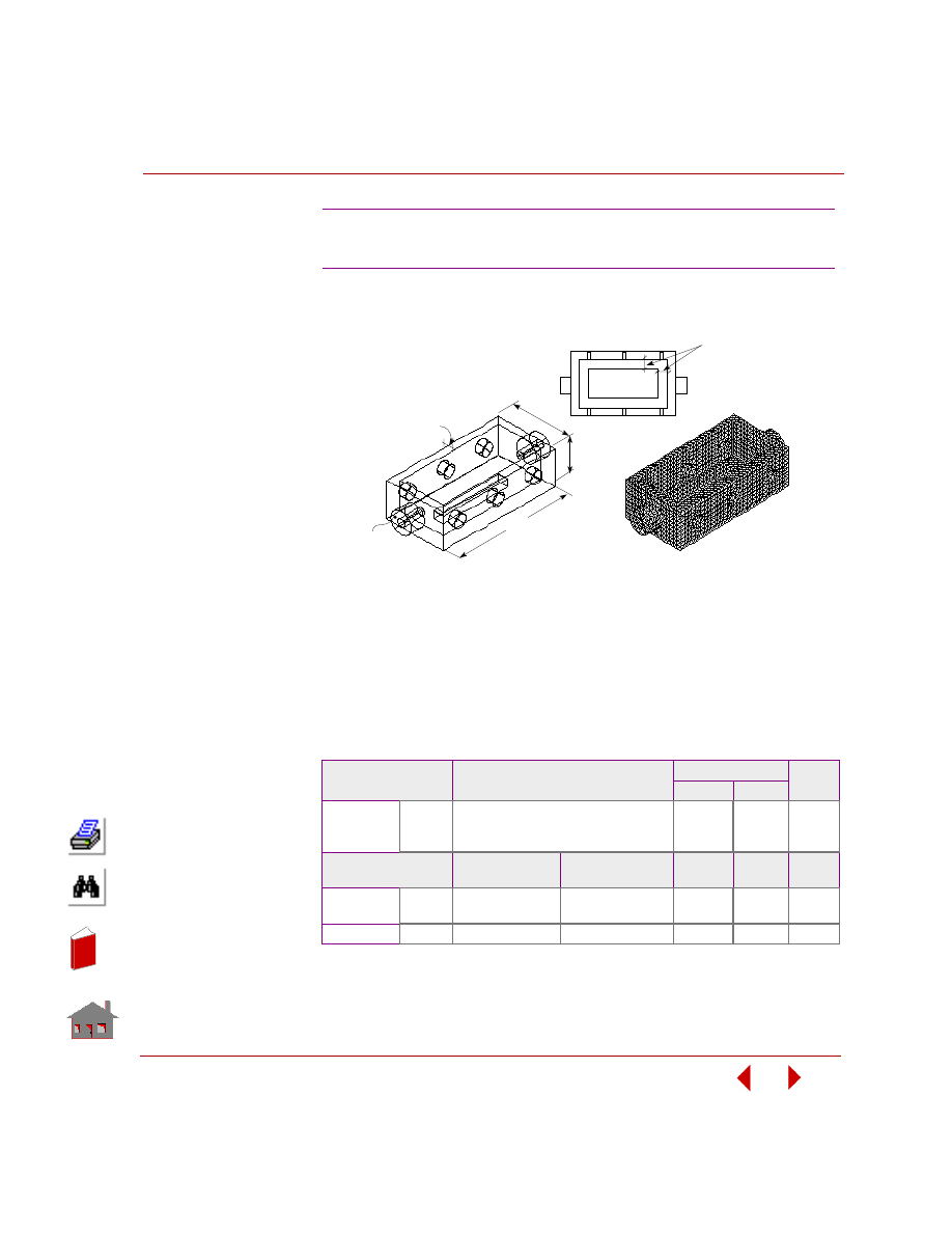
COSMOSM Advanced Modules
5-21
Part 2 OPSTAR / Optimization
KEYWORDS:
Shape, thermal analysis, TETRA10, minimum volume, and temperature constraint.
PROBLEM:
Find dimensions and thicknesses of the mechanical part. The material conductivity
is 0.57 W/mm-
°C. A convection of 0.0003 W/mm
2
-
°C with an ambient temperature
of 50
°C and a volume heat of 0.02 W/mm
3
are applied for the entire model. The
initial values and bounds of design variables, constraints and the objective function
are shown below.
SUMMARY OF RESULTS:
OPSHT3: Thermal Analysis of a
Simplified Mechanical Part
Optimization
Parameters
Initial Value(s) and Bounds
Final Value(s)
Toler-
ance
HSTAR
FFE
Design
Variables
TW
H
T
2
≤
6
≤
6
55
≤
100
≤
100
3
≤
15
≤
15
2.434
55.0
3.0
2.4367
55.0
3.0
0.04
0.45
0.12
Optimization
Parameters
HSTAR
FFE
HSTAR
FFE
Toler-
ance
Objective
Function
Volume
69405.3
69405.3
17030.75 17046.7
0.001
(Ratio)
Constraints
Temp 125
≤
222.5
≤
250 125
≤
222.27
≤
250 123.57
123.44
1.0
TW
H
TW
P la n
T
I nit ia l P roble m
G e ome t ry
I nit ia l Finit e
E le me nt Mode l
In
de
x
In
de
x
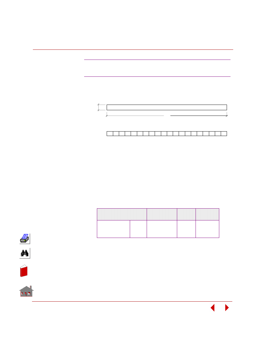
Chapter 5 Additional Problems
5-22
COSMOSM Advanced Modules
KEYWORDS:
Shape, transient thermal analysis, temperature-dependent conductivity, PLANE2D,
minimum volume, and temperature constraint.
PROBLEM:
Find the thickness of an infinitely large slab. The thermal conductivity K is assumed
to vary linearly with temperature, T
, (K = 2 + 0.01 T BTU/in-s °F). The specific heat
is constant (C = 8 BTU in/lb-s
2
°F). The temperature of the left side is suddenly
raised to 200
°F and returns to the initial temperature of 100 °F after 10 seconds. The
initial values and bounds of design variables, constraints and objective function are
shown below.
SUMMARY OF RESULTS:
OPSHT4: Transient Temperature –
Dependent Heat Conduction of a Slab
Optimization Parameters
Initial Value(s)
and Bounds
Final
Value(s)
Tolerance
Design Variables
H
5
≤
20
≤
20
5.6253
0.15
Objective Function
Volume
20
5.62531
0.01 (Ratio)
Constraints
Temp
0
≤
104.71
≤
150
151.47
1.50
H
Initial P roble m Ge ome try
Initial Finite E le me nt Me sh
1.0"
In
de
x
In
de
x
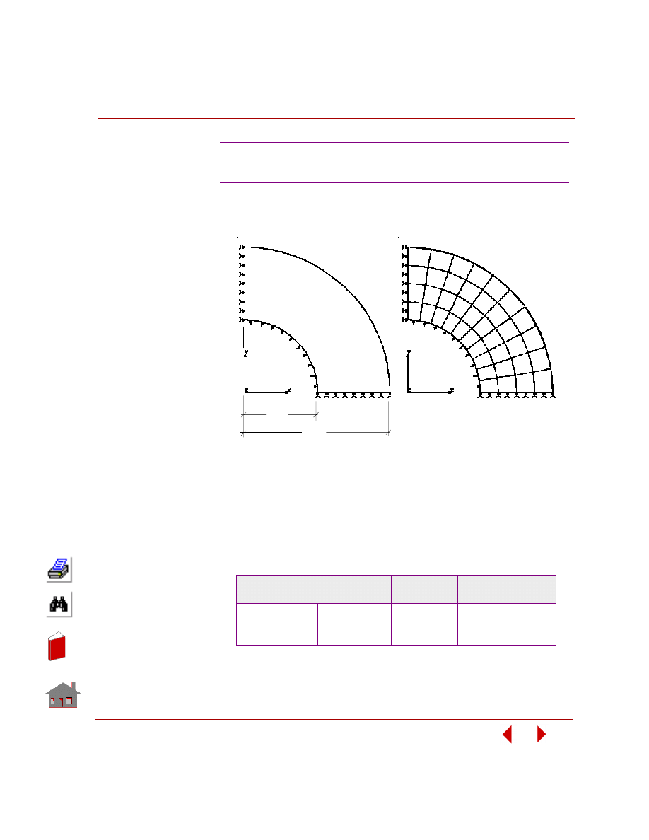
COSMOSM Advanced Modules
5-23
Part 2 OPSTAR / Optimization
KEYWORDS:
Shape, nonlinear analysis, von Mises plasticity, automatic time stepping,
PLANE2D, minimum volume, and stress constraint.
PROBLEM:
Find the pipe's outer diameter. The modulus of elasticity is 86,666 psi, Poisson's
ration is 0.3, yield stress is 17.32 psi and tangential modulus is 866 psi. The initial
values and bounds of design variables, constraints and objective function are shown
below.
SUMMARY OF RESULTS:
OPSN1: Nonlinear Analysis
of a Thick-walled Pipe
Optimization Parameters
Initial Value(s)
and Bounds
Final
Value(s)
Tolerance
Design Variables
ROUT
1.5
≤
2
≤
2.5
1.5427
0.01
Objective Function
Volume
2.34716
1.0795
0.01 (Ratio)
Constraints
von Mises stress
0
≤
17.396
≤
23
23.007
0.23
Rout
Initial P roble m Ge ome try
Rint
Initial Finite E le me nt Me sh
In
de
x
In
de
x
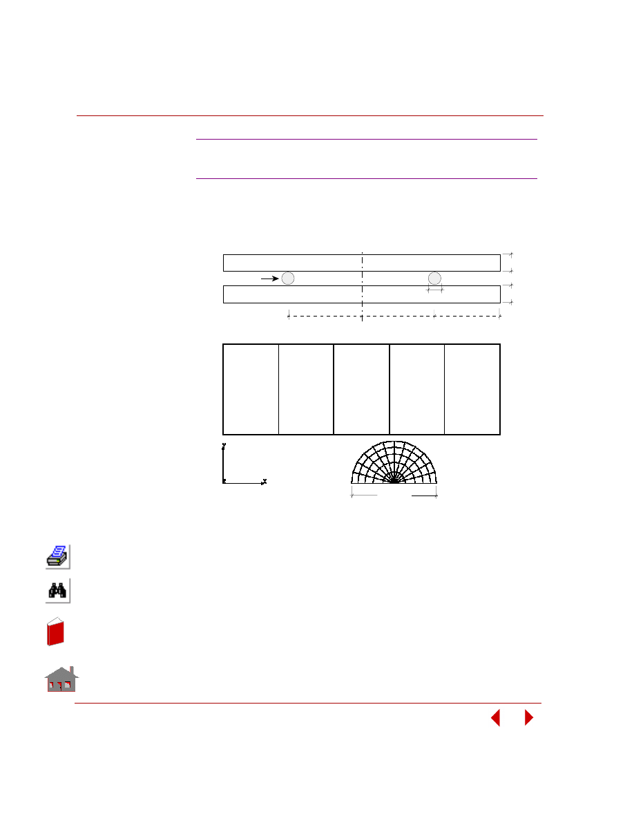
Chapter 5 Additional Problems
5-24
COSMOSM Advanced Modules
KEYWORDS:
Shape, nonlinear analysis, rubber, Mooney model, contact, prescribed displacement,
automatic time stepping, axisymmetric PLANE2D, minimum volume, and stress
constraint.
OPSN2: Nonlinear Analysis
of a Rubber Circular Ring
Initial Finite E le me nt Me sh
0.5615"
0.5615"
0.3475"
Top Steel Plate
Bottom Steel Plate
Initial P roble m Ge ome try
2 R Cross
0.3"
0.3"
0.278"
Rubber Ring
In
de
x
In
de
x

COSMOSM Advanced Modules
5-25
Part 2 OPSTAR / Optimization
PROBLEM:
Find the cross-section radius of a circular rubber ring squeezed between two parallel
steel plates. For rubber, the Mooney's constants are 175 and 10 psi and Poisson's
ratio is 0.49. For steal plates, the Young's modulus is 30 x 10
6
psi, and Poisson's ratio
is 0.30. The coefficient of friction is 0.01. The initial values and bounds of design
variables, constraints and objective function are shown below.
SUMMARY OF RESULTS:
Optimization Parameters
Initial Value(s)
and Bounds
Final
Value(s)
Tolerance
Design Variables
RCROSS
0.05
≤
0.139
≤
0.15
0.069462
0.001
Objective Function
Volume (rubber)
0.03
0.00749278
0.01 (Ratio)
Constraints
von Mises stress
0
≤
209.218
≤
450
453.37
4.5
In
de
x
In
de
x
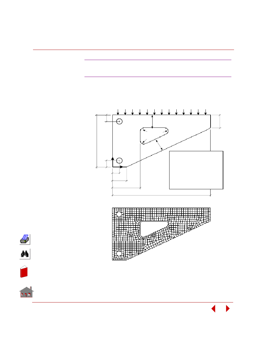
Chapter 5 Additional Problems
5-26
COSMOSM Advanced Modules
KEYWORDS:
Shape, static analysis, frequency analysis, multidisciplinary optimization, 8-node
PLANE2D, minimum volume, stress constraint, and frequency constraint.
OPSFS1: Stress and Frequency
Analysis of a Bracket
Note: All dimensions in milimeters.
100.
0
8 - Node P LANE 2 D
Me s h ( S iz e = 4 )
= 10 mm
= 5 N/mm
= 200,000 N/mm
2
2
= 0.3
= 0.00785 gm/mm
Thickness
Pressure
E
175.0
dv3
12.
5
25
dv2
dv1
Pressure
12.5
25
12.
5
Y
X
r = 5
r = 5
I nit ia l P roble m G e ome t ry
I nit ia l Finit e E le me nt Me s h
ν
Density
6
6
6
3
In
de
x
In
de
x
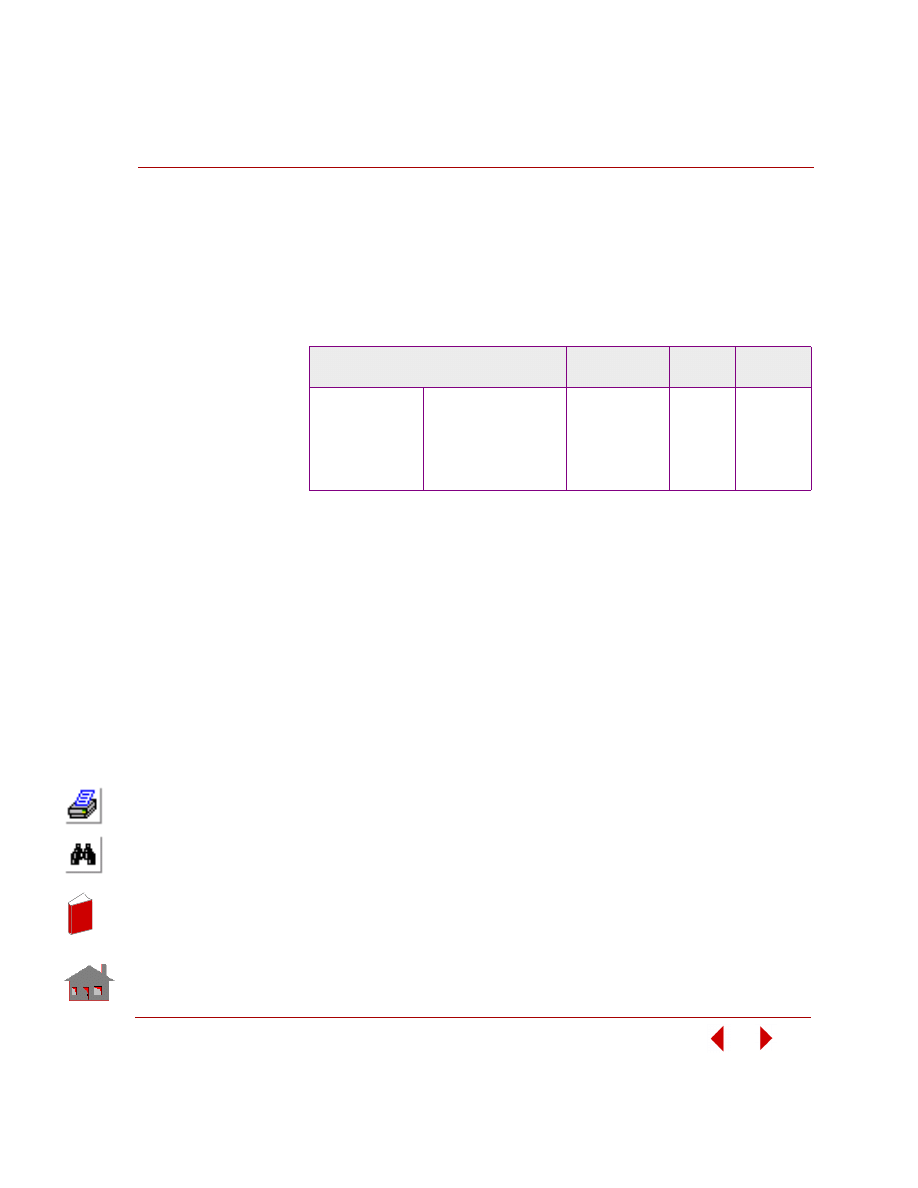
COSMOSM Advanced Modules
5-27
Part 2 OPSTAR / Optimization
PROBLEM:
Find size and location of the cutout. The bracket thickness is 10 mm, modulus of
elasticity is 200,000 N/mm
2
and Poisson's ratio is 0.3. A pressure of 5 N/mm
2
is
applied to the top edge of the bracket. The material density is 0.00785 gm/mm
3
.
The
initial values and bounds of design variables, constraints and the objective function
are shown below.
SUMMARY OF RESULTS:
Optimization Parameters
Initial Value(s)
and Bounds
Final
Value(s)
Tolerance
Design Variables
DV1
DV2
DV3
10
≤
25
≤
25
10
≤
25
≤
25
20
≤
50
≤
50
25.0
10.0
22.0
2.0
2.0
2.0
Objective Function
Volume
106,794
76,063.64
0.05 (Ratio)
Constraints
von Mises stress
Fundamental frequency
0
≤
94.12
≤
300
1.8
≤
2.8613
≤
3
241.52
1.7978
15.0
0.012
In
de
x
In
de
x
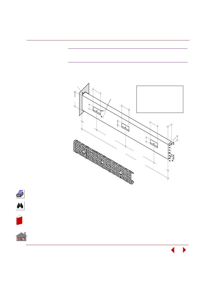
Chapter 5 Additional Problems
5-28
COSMOSM Advanced Modules
KEYWORDS:
Shape, stress analysis, buckling analysis, multidisciplinary optimization, SHELL3,
minimum volume, buckling load factor constraint, and stress constraint.
OPSBS1: Stress and Buckling
Analysis of a C-shape Column
I nit ia l Finit e
E le me nt Me s h
B = 20"
T
2
T
1
A = 6"
C = 3"
Fixed
T
2
T
1
T
2
T
1
h = 20"
0.18h
0.32h
0.32h
0.18h
p =
5,000 psi
(T /4)
2
Fillet
I nit ia l P roble m
G e ome t ry
= 3 in
= 0. 25 in
= A_ Steel
Element Size
Thickness
Material
S HE LL3
E
= 0.28
ν
= 3 x 10 psi
7
ρ
= 0.73 x 10 lbf sec /in
-3
2
4
In
de
x
In
de
x
COSMOSM Advanced Modules
5-29
Part 2 OPSTAR / Optimization
PROBLEM:
Find size of the column cutouts. The cross section thickness is 0.25 in., modulus of
elasticity is 3E7 psi, and Poisson's ratio is 0.28. A pressure of 5000 psi is applied to
the column's face. The initial values and bounds of design variables, constraints and
the objective function are shown below.
SUMMARY OF RESULTS:
Optimization Parameters
Initial Value(s)
and Bounds
Final
Value(s)
Tolerance
Design Variables
T1
T2
1
≤
5
≤
35
1
≤
5
≤
12
35.0
9.8635
0.34
0.11
Objective Function
Volume
1018.15
780.98
0.01 (Ratio)
Constraints
von Mises stress
Buckling load factor
0
≤
8,729
≤
22,000
1.8
≤
2.87
≤
10
19,125
1.8012
220
0.02
In
de
x
In
de
x
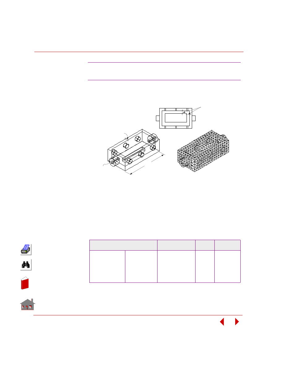
Chapter 5 Additional Problems
5-30
COSMOSM Advanced Modules
KEYWORDS:
Shape, static analysis, thermal analysis, multidisciplinary optimization, TETRA4R,
minimum volume, temperature constraint, and stress constraint.
PROBLEM:
Find dimensions and thicknesses of the mechanical part. The material conductivity
is 0.57 W/mm-
°C. A convection of 0.0003 W/mm
2
-
°C with an ambient temperature
of 50
°C and a volume heat of 0.02 W/mm
3
-
°C are applied for the entire model. The
modulus of elasticity is 1E07 N/mm
2
and Poisson's ratio is 0.30. The initial values
and bounds of design variables, constraints and the objective function are shown
below.
SUMMARY OF RESULTS:
OPSTS1: Stress and Thermal
Analysis of a Mechanical Part
Optimization Parameters
Initial Value(s)
and Bounds
Final
Value(s)
Tolerance
Design Variables
TW
H
T
2
≤
6
≤
6
55
≤
100
≤
100
3
≤
15
≤
15
2.4053
55.0
3.0
0.04
0.45
0.12
Objective Function
Volume
69,599.5
17,017.8
0.001 (Ratio)
Constraints
von Mises stress
Temperature
0
≤
8752.45
≤
9000
125
≤
222.658
≤
250
6133.8
123.18
20.0
2.0
TW
H
TW
P la n
T
Initial Finite E le me nt Me sh
Initial P roble m Ge ome try
In
de
x
In
de
x

COSMOSM Advanced Modules
5-31
Part 2 OPSTAR / Optimization
KEYWORDS:
Shape, thermal analysis, static analysis, frequency analysis, multidisciplinary
optimization, SHELL3,
TEMPREAD
command, minimum volume, temperature
constraint, displacement constraint, and frequency constraint.
OPSTSF1: Thermal, Static and Frequency
Analysis of a Circular Disk
Initial Finite E le me nt Me sh
25
10
5
= 2 mm
Thickness
3 - Node S he ll
Me s h ( S iz e = 2 )
10
5
5
5
2
Heat Flux
0.1 W/mm
Heat Flux
0.1 W/mm
2
Convection 0.0005 W/mm -
°
C
Ambient Temperature 50
°
C
2
Convection 0.0 W/mm -
°
C
Ambient Temperature 50
°
C
2
10
25
Radius
5
Initial P roble m Ge ome try
In
de
x
In
de
x
Chapter 5 Additional Problems
5-32
COSMOSM Advanced Modules
PROBLEM:
Find radius of the disk. The disk thickness is 2 mm, and conductivity is 0.57
W/mm
°C. A convection of 0.0005 W/mm
2
-
°C with an ambient temperature of 50 °C
is applied to the entire model except for the heat sources. The heat source regions
(heat flux of 0.1 W/mm
2
) is assumed to have a convection of 0 W/mm
2
-
°C with an
ambient temperature of 50
°C. The modulus of elasticity is 200000 N/mm
2
,
Poisson's ratio is 0.30, coefficient of thermal expansion is 0.13E-4/
°C and material
density is 0.00785 gm/mm
3
. The initial values and bounds of design variables,
constraints and the objective function are shown below.
SUMMARY OF RESULTS:
Optimization Parameters
Initial Value(s)
and Bounds
Final
Value(s)
Tolerance
Design Variables
Radius
30
≤
70
≤
70
38.859
1.0
Objective Function
Volume
33,251.96
11,955.40
0.0015 (Ratio)
Constraints
Temperature
Displ. frequency
Displ. frequency
50
≤
76.46
≤
140
0.09
≤
0.166
≤
0.17
1.0
≤
1.139
≤
8
107.39
0.08974
5.28985
1.0
0.0008
0.07
In
de
x
In
de
x
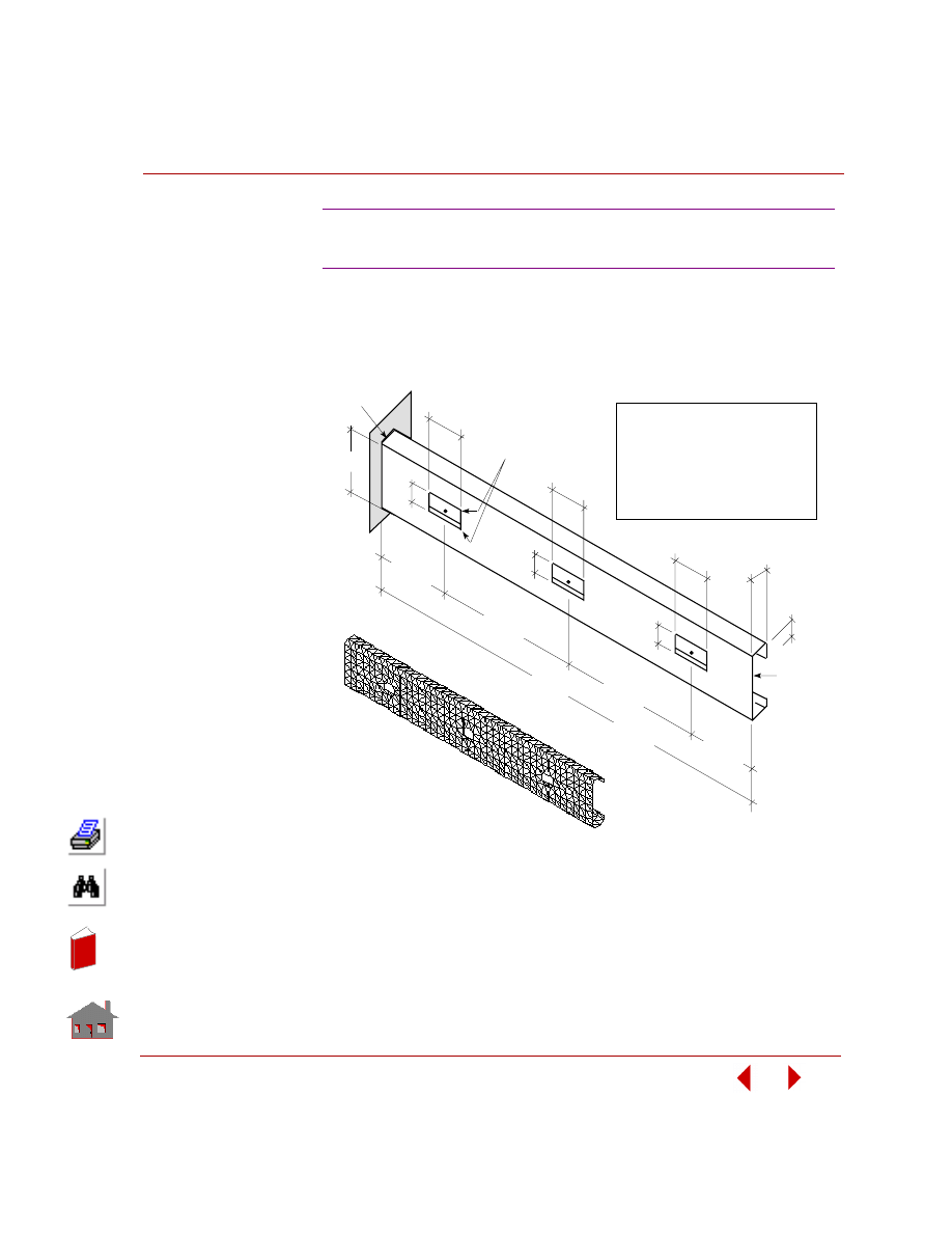
COSMOSM Advanced Modules
5-33
Part 2 OPSTAR / Optimization
KEYWORDS:
Shape, thermal analysis, static analysis, buckling analysis, multidisciplinary
optimization, SHELL3,
TEMPREAD
command, minimum volume, buckling load
factor constraint, and displacement constraint.
OPSTSB1: Thermal, Static and Buckling
Analysis of a Fixed Channel
I nit ia l Finit e
E le me nt Me s h
B = 20"
T
2
T
1
A = 6"
C = 3"
Fixed
T
2
T
1
T
2
T
1
h = 120"
0.18h
0.32h
0.32h
0.18h
(T /4)
2
Fillet
I nit ia l P roble m
G e ome t ry
= 3 in
= 0. 25 in
= A_ Steel
Element Size
Thickness
Material
S HE LL3
E
= 0.28
ν
= 3 x 10 psi
7
ρ
= 0.73 x 10 lbf sec /in
-3
2
4
Fixed
In
de
x
In
de
x
Chapter 5 Additional Problems
5-34
COSMOSM Advanced Modules
PROBLEM:
Find size of the channel cutouts. The cross section thickness is 0.25 in, modulus of
elasticity is 3E7 psi, and Poisson's ratio is 0.28.
The material conductivity is 6.7E-4 BTU/in/s/
°F. A convection of 0.0001 BTU/sec
in
2
-
°F with an ambient temperature of 50 °F and a volume heat of 0.005 BTU/sec in
3
are applied for the entire model. The material's coefficient of thermal expansion is
7.4E-6/
°F The initial values and bounds of design variables, constraints and the
objective function are shown below.
SUMMARY OF RESULTS:
Optimization Parameters
Initial Value(s)
and Bounds
Final
Value(s)
Tolerance
Design Variables
T1
T2
1
≤
5
≤
35
1
≤
5
≤
12
17.257
12.00
0.34
0.11
Objective Function
Volume
1018.15
887.157
0.01 (Ratio)
Constraints
Buckling factor
Displacement
1.6
≤
1.8432
≤
10
0.0
≤
0.01102
≤
0.018
3.981
0.018179
0.02
0.00018
In
de
x
In
de
x
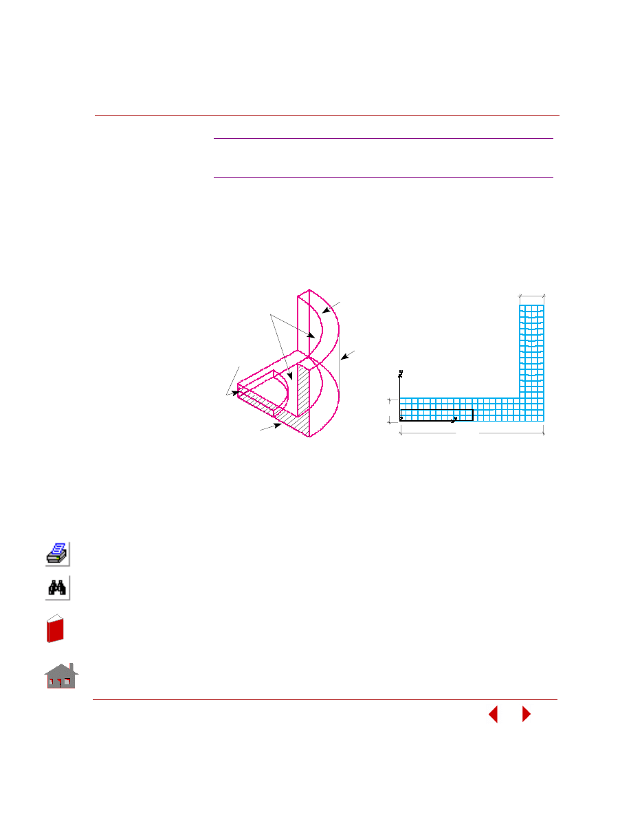
COSMOSM Advanced Modules
5-35
Part 2 OPSTAR / Optimization
KEYWORDS:
Shape, transient thermal, nonlinear analysis, radiation, convection, heat flux;
element heat, prescribed temperature, multi-disciplinary optimization, von Mises
plasticity, Axisymmetric PLANE2D, minimum volume, stress, strain and
temperature constraints.
PROBLEM:
Find the radius and thickness of a cylinder subject to thermal loads and boundary
conditions. Steel alloy and Aluminum materials are used. The initial values and
bounds of design variables, constraints and objective function are shown below.
OPSTN1: Transient Thermal –
Nonlinear Analysis of a Cylinder
Thick
Initia l Finite Ele me nt Me sh
Initia l Ge ome try, Loa ds
a nd Bounda ry C onditions
Thick
ROUT
Temperature = 70
°
F
Radiation Source
Emissivity
View Factor
= 500
°
F
= 0.9
= 0.8
Ambient
Temperature = 200
°
F
Firm Coefficient
= 0.1 BTU /
(sec in in
°
F)
_
Convection
Element
Heat
= 0.140625 BTU /
(sec in in in)
Heat Flux
= 0.0125 BTU /
(sec in in)
In
de
x
In
de
x
Chapter 5 Additional Problems
5-36
COSMOSM Advanced Modules
SUMMARY OF RESULTS:
Optimization Parameters
Initial Value(s)
and Bounds
Final
Value(s)
Tolerance
Design Variables
ROUT
THICK
5
≤
12
≤
12
0.5
≤
2
≤
2
5
0.66144
0.07
0.015
Objective Function
Volume
39.999
9.4841
0.01 (Ratio)
Constraints
von Mises 1
von Mises 2
Temp
Effective Strain 1
Effective Strain 2
0
≤
44,045
≤
50,000
0
≤
30,213
≤
30,000
350.
≤
413.63
≤
450
0
≤
0.003896
≤
0.01
0
≤
0.0021032
≤
0.01
38954.81
30152.49
381.429
0.003445
0.001796
500
300
1.0
1 x 10
-4
1 x 10
-4
In
de
x
In
de
x
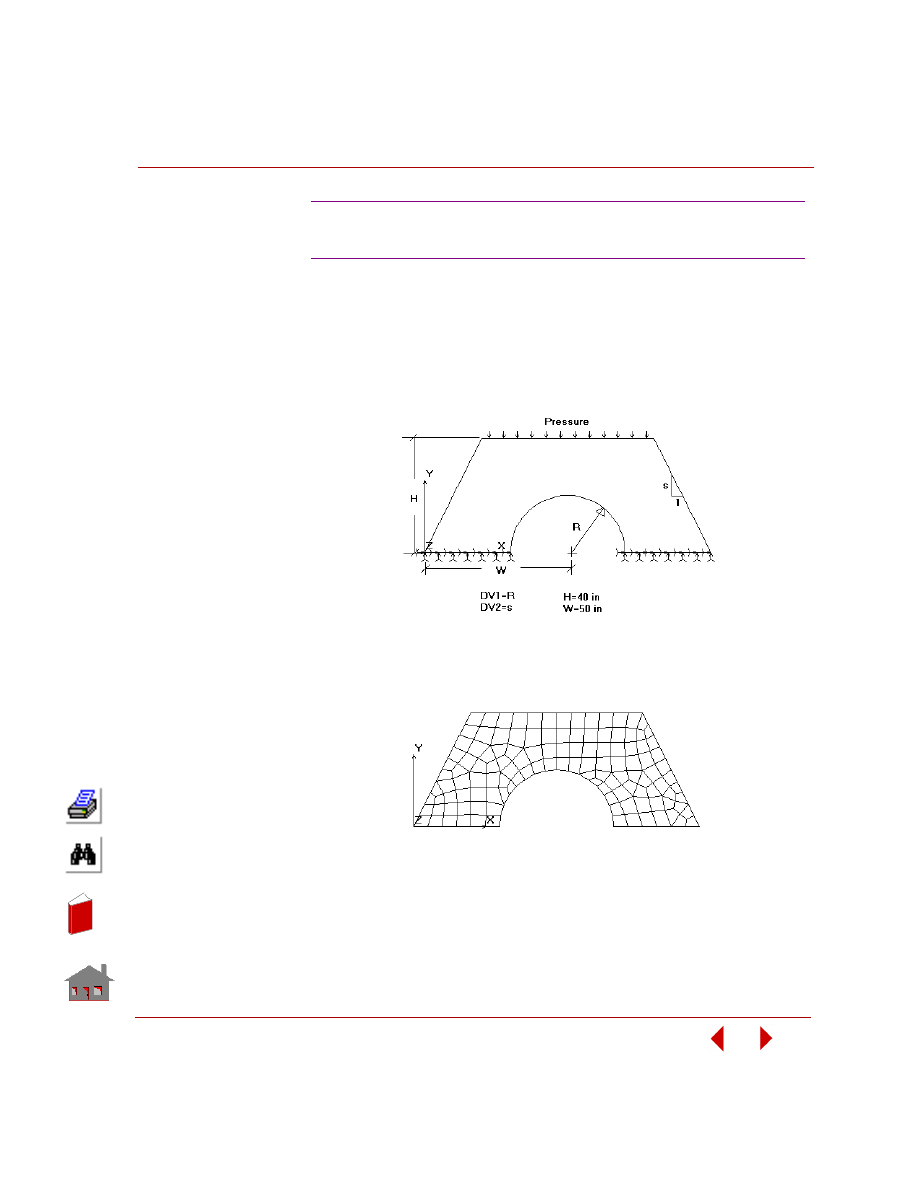
COSMOSM Advanced Modules
5-37
Part 2 OPSTAR / Optimization
KEYWORDS:
Frequency analysis, post-dynamic analysis (harmonic response), dynamic stress
analysis, 4-noded PLANE2D elements, shape optimization, multidisciplinary
optimization, minimum volume design, frequency, displacement, and stress
constraints.
Initial Problem Geometry
Initial Finite Element Mesh
OPSFDS1: Harmonic Response
Analysis of a Culvert
In
de
x
In
de
x

Chapter 5 Additional Problems
5-38
COSMOSM Advanced Modules
PROBLEM:
Find the radius R and slope s of a culvert. The material constants of the culvert are
given as: Young’s modulus E = 30E6 psi, Poisson’s ratio
υ = 0.3, and Density ρ = 1
lb*sec
2
/in
4
. A harmonic pressure loading with constant amplitude 500 psi within the
desired range of frequency (1 rad/sec - 400 rad/sec) is applied to the top of the
culvert. A modal damping 0.015 is assumed for the first 10 modes. The input data
regarding optimization as well as the converged results are listed in the following
table. Note that the displacement and stress constraints are defined as the extreme
values within the desired range of frequency.
SUMMARY OF RESULTS:
Optimization Parameters
Initial Value(s)
and Bounds
Final
Value(s)
Tolerance
Design Variables
DV1
DV2
20
≤
20
≤
35
1.3333
≤
2
≤
2
23.268
1.3333
0.15
6.6667E-3
Objective Function
Volume
2575.5
1954.8
0.01 (ratio)
Constraints
Frequency (1st)
Displacement (Uy)
Stress (von Mises)
5
≤
16.179
≤
20
0
≤
0.0429
≤
0.05
0
≤
4.6893E4
≤
5E4
15.470
0.05021
4.7637E4
0.15
5.E-4
500.
In
de
x
In
de
x
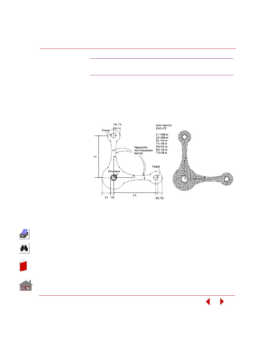
COSMOSM Advanced Modules
5-39
Part 2 OPSTAR / Optimization
KEYWORDS:
Frequency analysis, post-dynamic analysis (random vibration), dynamic stress
analysis, 6-noded TRIANG elements, shape optimization, multidisciplinary
optimization, minimum volume design, frequency, displacement, and stress
constraints.
OPSFDS2: Random Vibration
Analysis of a Lever Arm
Initial Problem Geometry
Initial Finite
Element Mesh
In
de
x
In
de
x
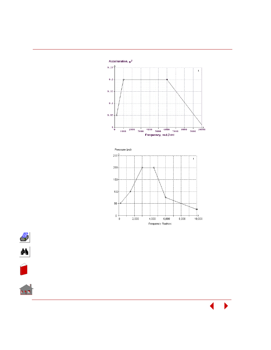
Chapter 5 Additional Problems
5-40
COSMOSM Advanced Modules
Base Excitation versus Frequency Curve
Pressure Loading versus Frequency Curve
In
de
x
In
de
x
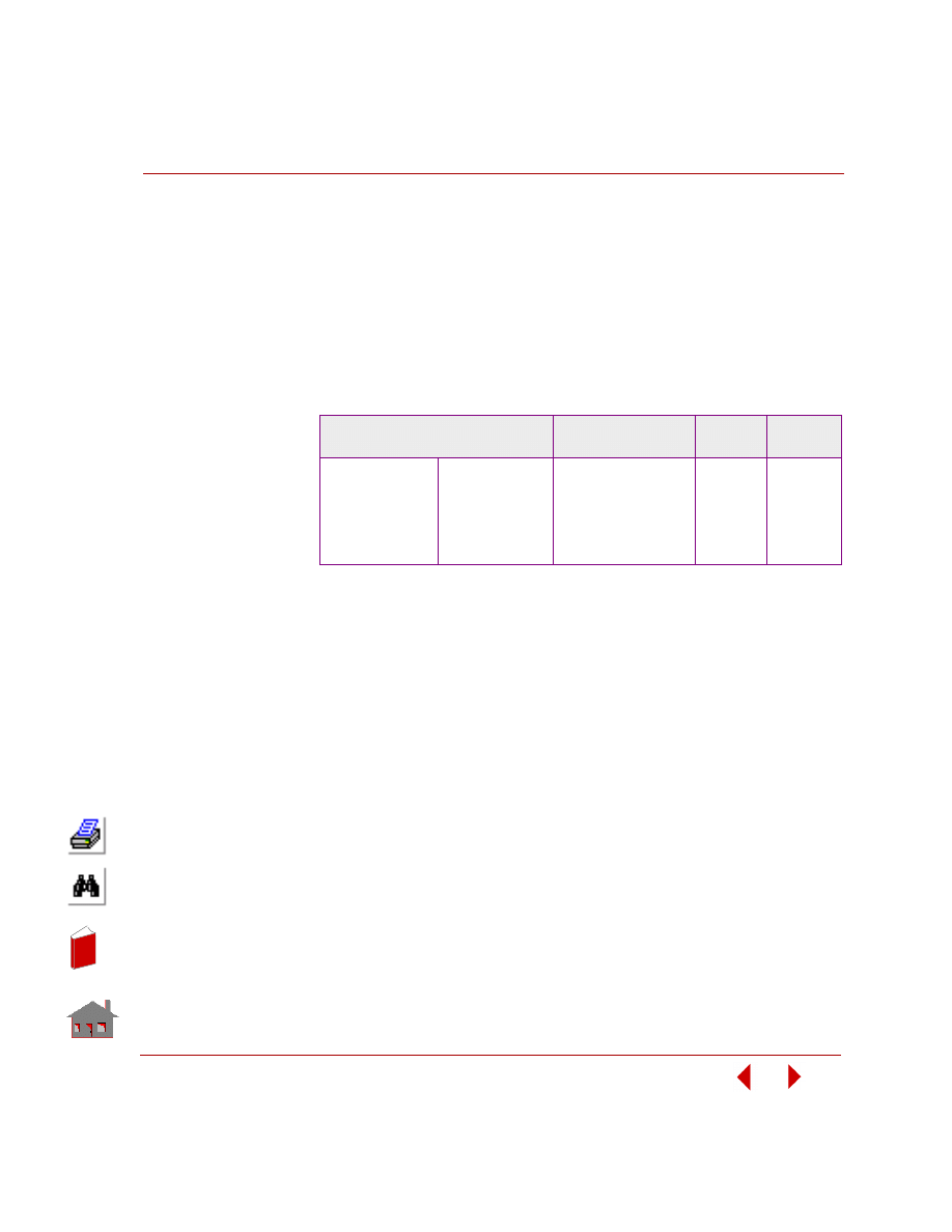
COSMOSM Advanced Modules
5-41
Part 2 OPSTAR / Optimization
PROBLEM:
Find the hyperbolic arc parameter RATIO and thickness T2 of a lever arm. The arm
is made of A_STEEL and has a uniform thickness 1.0 in. Both harmonic pressure
loading and base excitation (acceleration) in the y-direction are applied to the
structure as shown in the figure. A modal damping 3% is assumed for the first 5
modes. The input data regarding optimization as well as the converged results are
listed in the following table. Note that the displacement constraint is defined as the
extreme value of PSD within the desired range of frequency and the stress constraint
is the extreme value of RMS.
SUMMARY OF RESULTS:
Optimization Parameters
Initial Value(s)
and Bounds
Final
Value(s)
Tolerance
Design Variables
DV1
DV2
0.5
≤
0.5
≤
0.75
15
≤
40
≤
50
0.6325
29.782
2.5E-3
0.35
Objective Function
Volume
2.008E4
1.6078
0.01 (ratio)
Constraints
Frequency (1st)
Displacement (Uy)
Stress (von Mises)
75
≤
92.377
≤
100
0
≤
3.1874E-5
≤
3.5E-5
0
≤
1.1893E4
≤
1.25E4
82.089
2.1262E-5
1.2624E4
0.25
3.5.E-7
125.
In
de
x
In
de
x
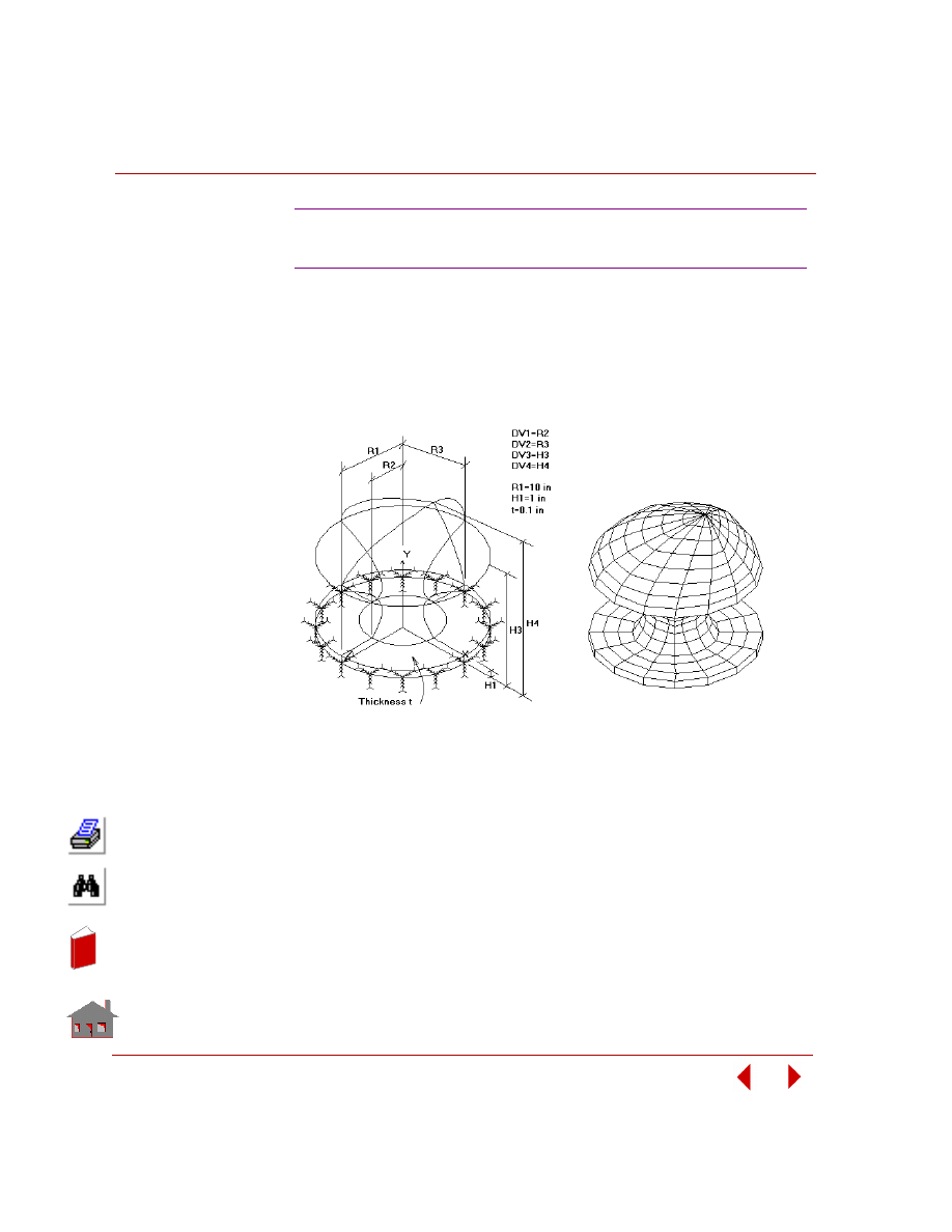
Chapter 5 Additional Problems
5-42
COSMOSM Advanced Modules
KEYWORDS:
Frequency analysis, post-dynamic analysis (time history analysis, response
spectrum generation, and response spectrum analysis), dynamic stress analysis,
SHELL4 elements, shape optimization, multidisciplinary optimization, maximum
volume design, frequency, displacement, and stress constraints.
OPSFDS3: Response Spectrum
Analysis of a Trophy Setting on a Table
Initial Problem Geometry
Initial Finite Element Mesh
In
de
x
In
de
x
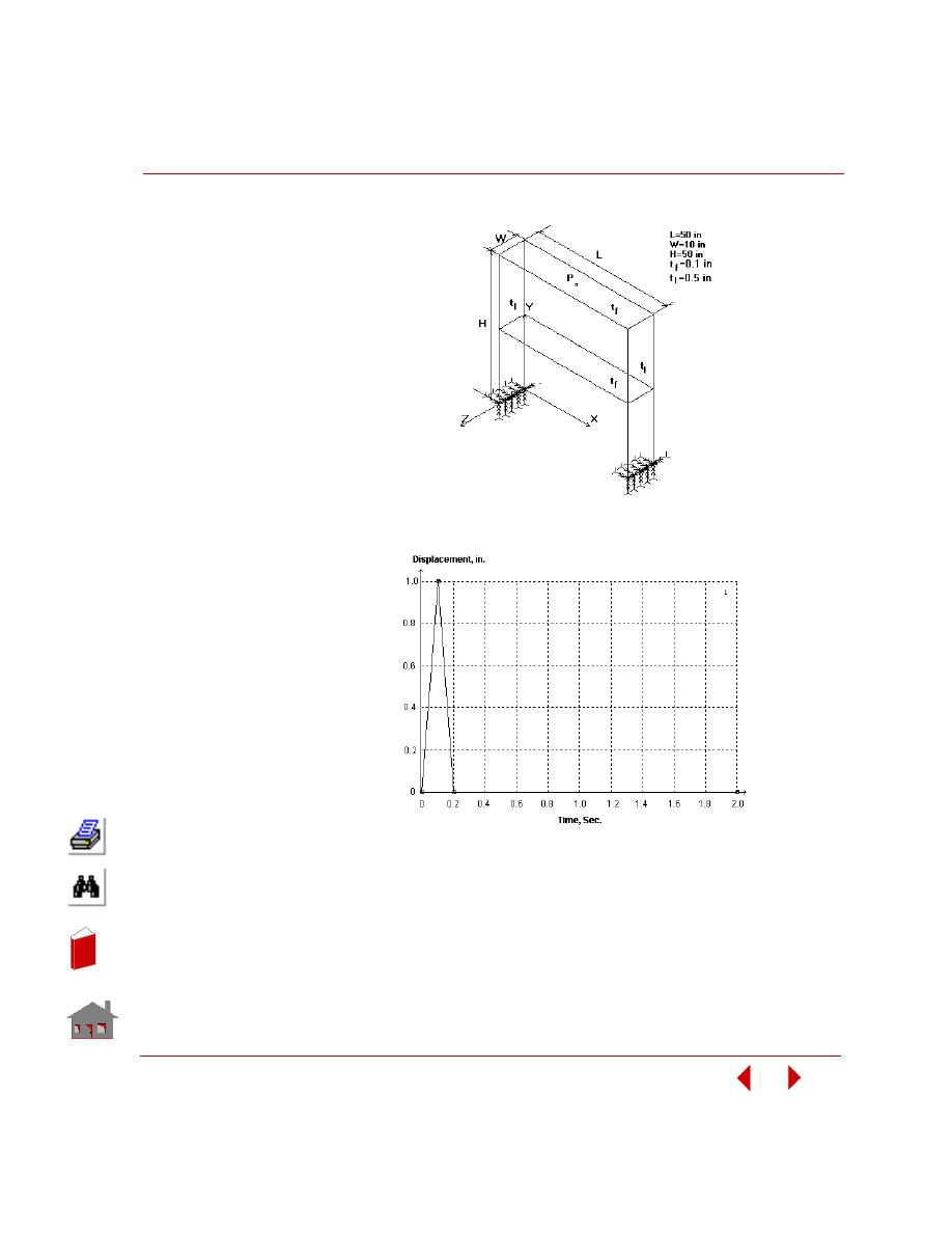
COSMOSM Advanced Modules
5-43
Part 2 OPSTAR / Optimization
Geometry of a Table
Impulsive Base Excitation (for Table)
In
de
x
In
de
x
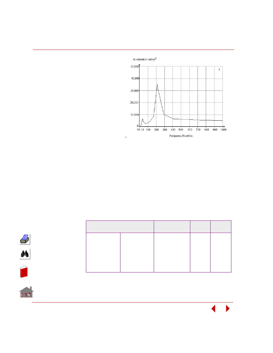
Chapter 5 Additional Problems
5-44
COSMOSM Advanced Modules
PROBLEM:
Find the radii (R2
and R3) and heights
(H3 and H4) of a
trophy which is
setting on the top
level of a table at the
point P. Both
structures are made
of A_STEEP. The
trophy has a 5%
critical damping.
This problem is
solved in three
steps:
1.
A time history
analysis of the
table is performed where an impulsive displacement base excitation in the x-
direction is applied.
2.
A maximum acceleration response spectrum is generated from the previous
results.
3.
A design optimization of the trophy in the response spectrum analysis is per-
formed where the spectrum generated previously is used to excite the trophy in
the form of acceleration base excitation.
The input data regarding optimization as well as the converged results are listed in
the following table. Note that the displacement and stress constraints are defined as
the extreme values by using the SRSS mode combination method.
SUMMARY OF RESULTS:
Optimization Parameters
Initial Value(s)
and Bounds
Final
Value(s)
Tolerance
Design Variables
DV1
DV2
DV3
DV4
4
≤
5
≤
8
8
≤
10
≤
20
8
≤
10
≤
15
15
≤
20
≤
25
4.994
20
8
25
0.04
0.12
0.07
0.1
Objective Function
Volume
377.49
1229.75
0.01 (ratio)
Constraints
Frequency (1st)
Displacement (Ux)
Stress (von Mises)
10
≤
27.043
≤
40
0
≤
0.3549
≤
0.5
0
≤
1.849E4
≤
2.5E4
10.935
0.5019
1.9645E4
0.3
0.005
250
Maximum Response Spectrum Generation (for Trophy)
In
de
x
In
de
x
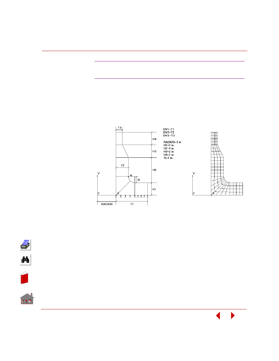
COSMOSM Advanced Modules
5-45
Part 2 OPSTAR / Optimization
KEYWORDS:
Transient thermal analysis, nonlinear elastoplastic analysis, fatigue analysis, 4-
noded PLANE2D elements, shape optimization, multidisciplinary optimization,
minimum volume design, fatigue usage factor, displacement, and stress constraints.
OPSTNFT1: Fatigue Analysis of a Nozzle
Under a Cyclic Temperature Loading
Initial Problem Geometry
Initial Finite Element Mesh
In
de
x
In
de
x
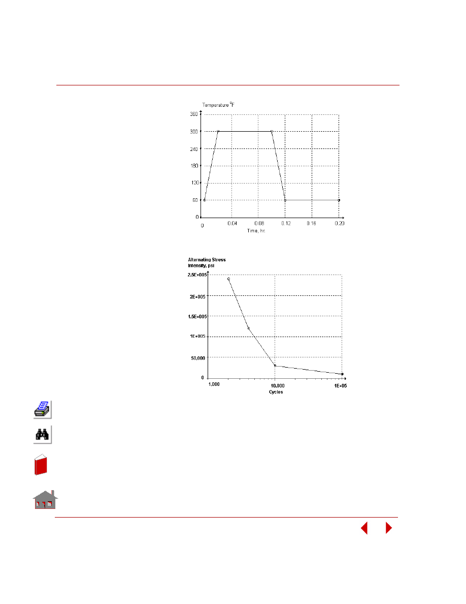
Chapter 5 Additional Problems
5-46
COSMOSM Advanced Modules
Temperature Variation Cycle
Fatigue Design Curve (S-N Curve)
In
de
x
In
de
x
COSMOSM Advanced Modules
5-47
Part 2 OPSTAR / Optimization
PROBLEM:
Find the thickness parameters T1, T2, and T3 of a circular nozzle. The material
constants of the nozzle are given as: Young’s modulus E = 3E7 psi, Poisson’s ratio
υ =0.3, density ρ = 3E-4 lb*hr
2
/in
4
, yield stress
σ
y
= 1E4 psi, tangent modulus E
T
=
3E6 psi, coefficient of thermal expansion
α = 8E-6 1/°F, thermal conductivity K
x
=
0.1 BTU/(in*hr*
°F), and specific heat C = 40 BTU*in/(lb*hr
2
*
°F). The convection
coefficient h and the adjacent ambient temperature T
a
for the exterior and interior
surfaces of the nozzle are 1 and 5 BTU/(in
2
*hr*
°F) and 60 and 1 °F, respectively.
Assuming that the nozzle is exposed to a fluid heat-up condition which is expected
to occur 5000 times during its service life. One complete cycle of this heat-up
condition is shown in the figure. The problem is solved in three steps:
1.
A transient thermal analysis is performed with the initial temperature T
0
equal
to 60
°F. The nodal temperatures of the structure are evaluated at each time
interval 0.01 hours for a total time 0.2 hours.
2.
Applying the nodal temperatures obtained from the transient thermal analysis to
the structure, a nonlinear elastoplastic analysis is performed. The reference tem-
perature Tref is 60
°F.
3.
With the stresses obtained from the nonlinear analysis, a fatigue analysis is per-
formed. A specified fatigue design curve (S-N curve) is shown in the figure.
The input data regarding optimization as well as the converged results are listed in
the following table. Note that the constraints, fatigue usage factor and von Mises
stress, are estimated at node N on the exterior surface of the nozzle and the resultant
displacement is defined as the extreme value within the desired range of time (0 - 0.2
hours).
SUMMARY OF RESULTS:
Optimization Parameters
Initial Value(s) and
Bounds
Final
Value(s)
Tolerance
Design Variable
DV1
DV2
DV3
3 < 5 < 5
1 < 2 < 2
0.25 < 1 < 1
3.0
1.1708
0.25
0.02
0.01
7.5E-3
Objective
Function
Volume
23.219
12.824
0.01 (ratio)
Constraints
Fatigue Usage Factor
Displacement (Ures)
Stress (von Mises)
0 < 0.1030 < 0.15
0 < 0.01057 < 0.012
0 < 1.1523E4 < 1.5E4
0.1491
0.01144
1.5116E4
1.5E-3
1.2E-4
150
In
de
x
In
de
x
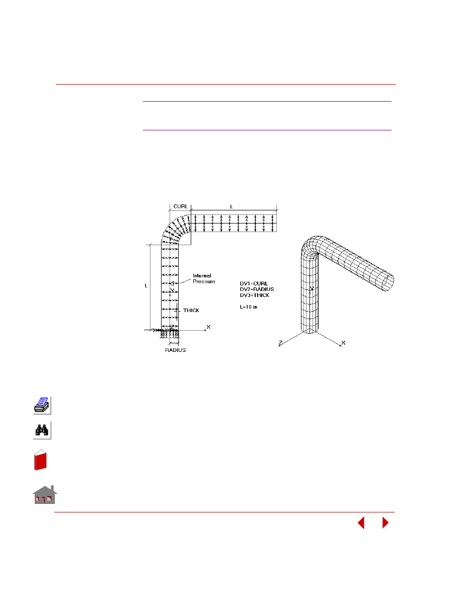
Chapter 5 Additional Problems
5-48
COSMOSM Advanced Modules
KEYWORDS:
Frequency analysis, post-dynamic analysis (modal time history), dynamic stress
analysis, fatigue analysis, SHELL4 elements, shape/sizing optimization,
multidisciplinary optimization, minimum volume design, frequency, fatigue usage
factor, displacement, and stress constraints.
OPSFDSFT1: Fatigue Analysis of a Curved
Pipe Under a Cyclic Pressure Loading
Initial Problem Geometry
Initial Finite Element Mesh
In
de
x
In
de
x
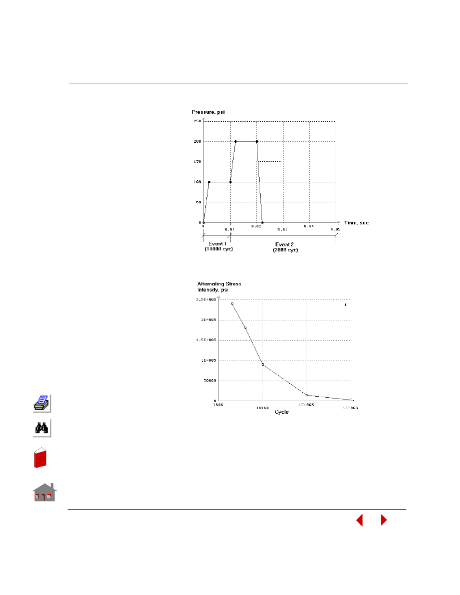
COSMOSM Advanced Modules
5-49
Part 2 OPSTAR / Optimization
Pressure Variation Cycle
Fatigue Design Curve (S-N Curve)
In
de
x
In
de
x
Chapter 5 Additional Problems
5-50
COSMOSM Advanced Modules
PROBLEM:
Find the dimension parameters CURL, RADIUS, and thickness THICK of a curved
pipe. The pipe is made of A_STEEL. A varying internal pressure loading is applied
to the pipe which is expected to occur 10000 and 2000 times during its service life.
One complete cycle of this loading is shown in the figure. The problem is solved in
two steps:
1.
A modal time history analysis of the pipe is performed with the prescribed pres-
sure loading. A modal damping 0.05 is assumed for the first 5 modes. The
responses during a total range of time 0.05 sec are recorded.
2.
With the stresses obtained from the dynamic stress analysis, a fatigue analysis is
performed. A specified fatigue design curve (S-N curve) is shown in the figure.
The input data regarding optimization as well as the converged results are listed in
the following table. Note that the constraint, fatigue usage factor, is the extreme
value among all the nodes and the resultant displacement and von Mises stress are
defined as the extreme value within the desired range of time (0 - 0.05 sec).
SUMMARY OF RESULTS:
Optimization Parameters
Initial Value(s) and
Bounds
Final
Value(s)
Tolerance
Design Variable
DV1
DV2
DV3
1.5
≤
2.5
≤
2.5
0.25
≤
1
≤
1
0.05
≤
0.1
≤
0.1
1.5
0.25
0.0739
0.01
7.5E-3
5.E-4
Objective Function
Volume
14.930
2.5789
0.01 (ratio)
Constraints
Frequency (1st)
Fatigue Usage Factor
Displacement (U
res
)
Stress (von Mises)
50
≤
146.28
≤
150
0
≤
0.07713
≤
0.15
0
≤
0.1122
≤
0.3
0
≤
2.7786E4
≤
5E4
50.882
0.1085
0.3012
2.8889E4
1
1.5E-3
3.E-3
500
In
de
x
In
de
x
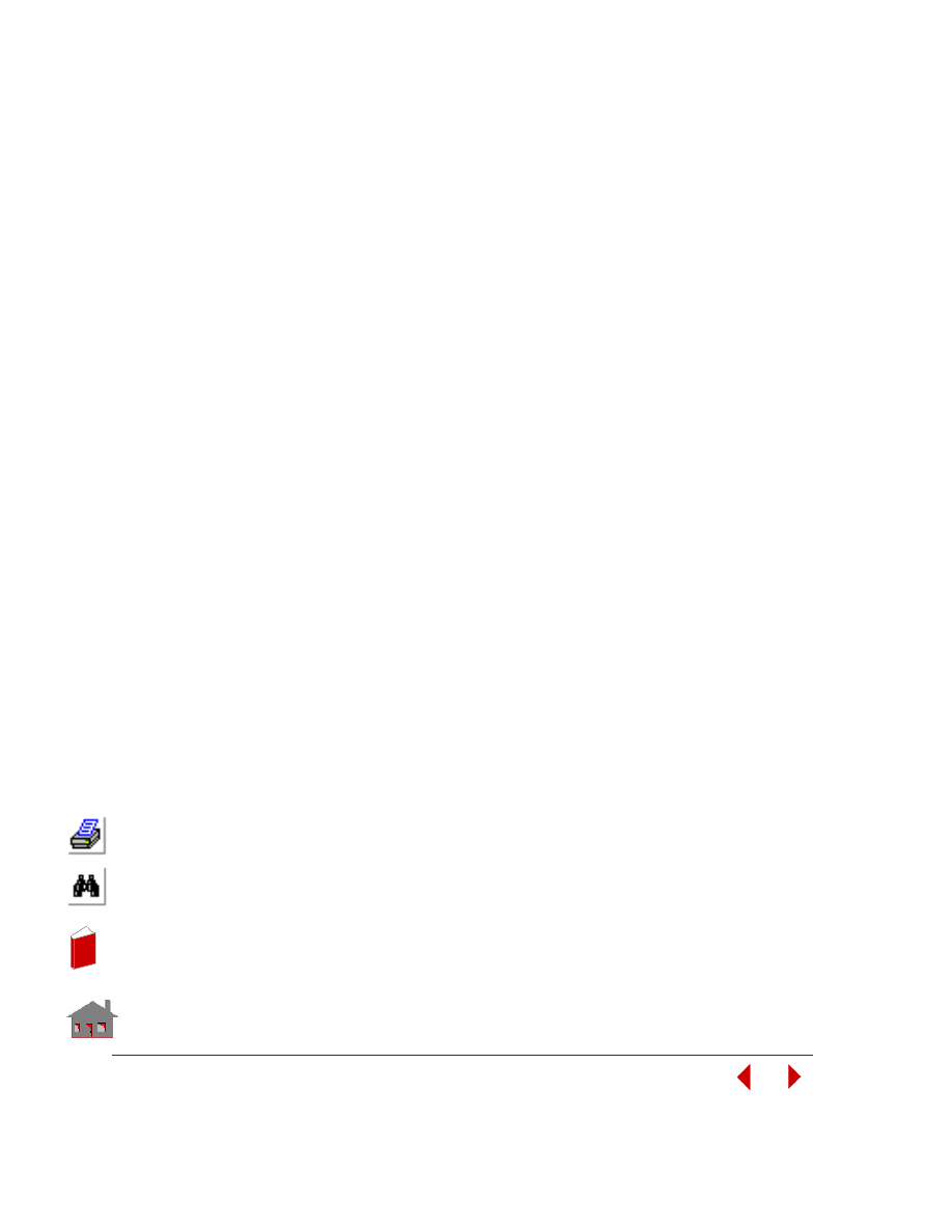
COSMOSM Advanced Modules
5-51
Sizing Optimization
Problems
In
de
x
In
de
x
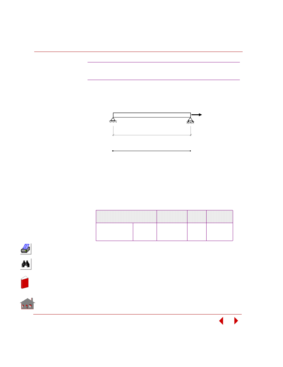
Chapter 5 Additional Problems
5-52
COSMOSM Advanced Modules
KEYWORDS:
Sizing, static analysis, TRUSS2D, minimum volume, and stress constraint.
PROBLEM:
Find the minimum volume of a 1-bar truss subject to a concentrated force of 10 lb.
The length of the bar is 1 in. and modulus of elasticity is 5 psi. The initial values and
bounds of design variables, constraints and the objective function are shown below.
SUMMARY OF RESULTS:
OPZST1: Minimum Volume of a 1-bar
Truss Subject to Stress Constraint
Optimization Parameters
Initial Value(s)
and Bounds
Final
Value(s)
Tolerance
Design Variables
A1
0.25
≤
1.0
≤
1.0
0.50005
0.0075
Objective Function
Volume
1.0
0.50005
0.001 (Ratio)
Constraints
Max stress
0.5
≤
10
≤
20
19.998
0.00001
E = 5 psi
F = 10 lbs
1"
A
1
Finit e E le me nt Me s h
P roble m G e ome t ry
Area =
In
de
x
In
de
x
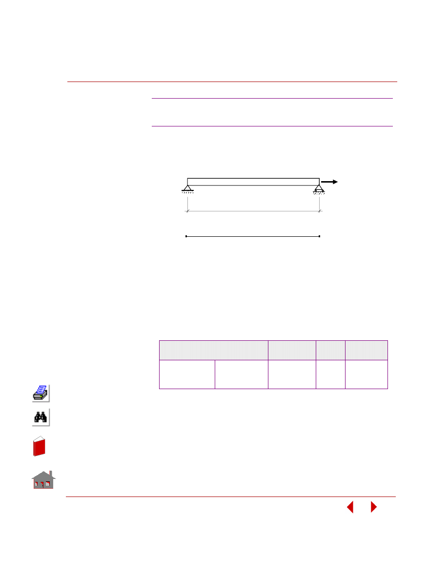
COSMOSM Advanced Modules
5-53
Part 2 OPSTAR / Optimization
KEYWORDS:
Sizing, static analysis, TRUSS2D, minimum volume, and displacement constraint.
PROBLEM:
Find the minimum volume of a 1-truss element subject to a concentrated force of 10
lb. The length of the bar is 1 in. and modulus of elasticity is 5 psi. The initial values
and bounds of design variables, constraints and the objective function are shown
below.
SUMMARY OF RESULTS:
OPZST2: Minimum Volume of a 1-bar
Truss Subject to Displacement Constraint
Optimization Parameters
Initial Value(s)
and Bounds
Final
Value(s)
Tolerance
Design Variables
A1
0.25
≤
1.0
≤
1.0
0.49776
0.0075
Objective Function
Volume
1.0
0.49776
0.001 (Ratio)
Constraints
Max displacement
1
≤
2
≤
4
4.018
0.03
E = 5 psi
F = 10 lbs
1"
A
1
Finit e E le me nt Me s h
P roble m G e ome t ry
Area =
In
de
x
In
de
x
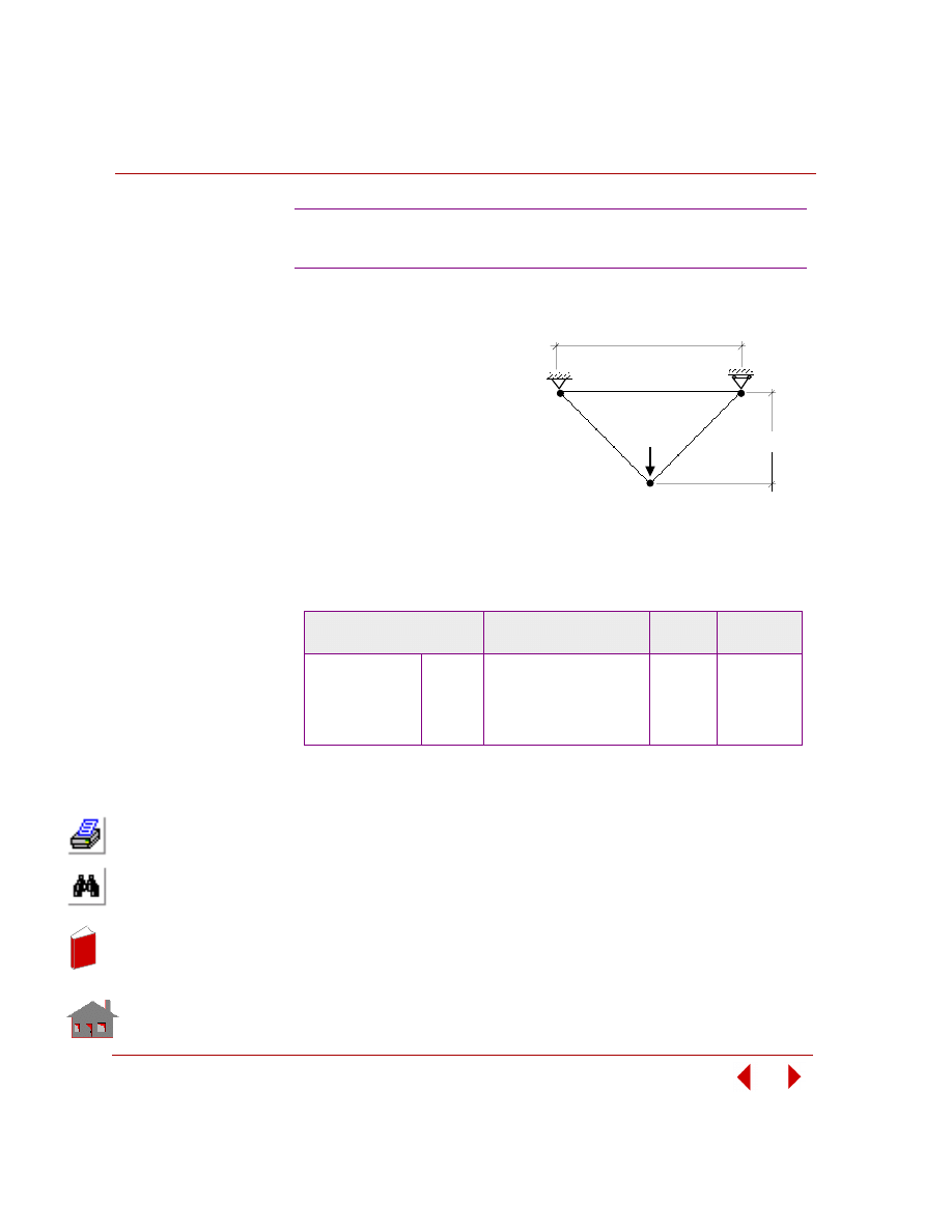
Chapter 5 Additional Problems
5-54
COSMOSM Advanced Modules
KEYWORDS:
Sizing, static analysis, TRUSS2D,
minimum volume, and stress
constraint.
PROBLEM:
Find the minimum volume of a 3-
bar truss subject to a concentrated
force of 20,000 lb. The modulus of
elasticity is 1E7 psi. The initial
values and bounds of design
variables, constraints and the
objective function are shown
below.
SUMMARY OF RESULTS:
OPZST3: Minimum Volume of a 3-bar Statically
Determinate Truss Subject to Stress Constraints
Optimization Parameters
Initial Value(s)
and Bounds
Final
Value(s)
Tolerance
Design Variables
A1 = A2
A3
0.50
≤
2.0
≤
4.0
0.50
≤
1.0
≤
4.0
0.70394
0.66342
0.001
0.001
Objective Function
Volume
76.5685
33.179
0.025 (Ratio)
Constraints
σ
x
1, 2
σ
x
3
-15,000
≤
7,071
≤
20,000
-15,000
≤
-10,000
≤
20,000
20,090
-15,073
150
150
20,000 lbs
20"
A
3
A
1
A
2
P roble m G e ome t ry
10"
In
de
x
In
de
x
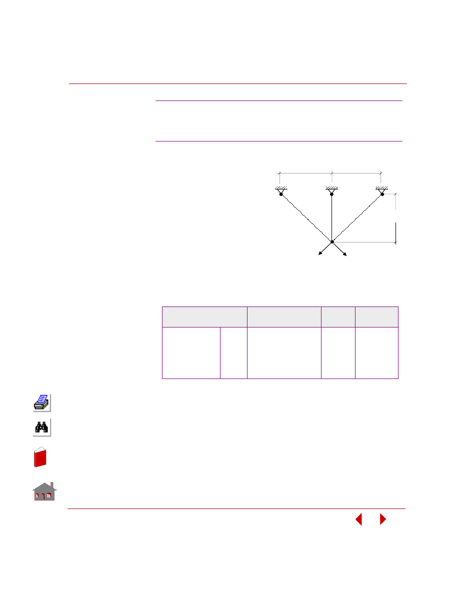
COSMOSM Advanced Modules
5-55
Part 2 OPSTAR / Optimization
KEYWORDS:
Sizing, static analysis, TRUSS2D,
minimum weight, and stress
constraint, and multiple load cases.
PROBLEM:
Find the minimum weight of a 3-bar
truss subject to concentrated forces of
20,000 lb applied in two distinct load
cases. The modulus of elasticity is
1E7 psi. The initial values and bounds
of design variables, constraints and
the objective function are shown
below.
SUMMARY OF RESULTS:
OPZST4: Minimum Weight of a 3-bar Statically
Indeterminate Truss Subject to Stress
Constraints – Multiple Load Cases
Optimization Parameters
Initial Value(s)
and Bounds
Final
Value(s)
Tolerance
Design Variables
A1
A2
0.10
≤
1.0
≤
100
0.10
≤
2.0
≤
100
0.7147
0.6665
0.01
0.01
Objective Function
Weight
4.8284
2.6881
0.001 (Ratio)
Constraints
σ
x
1
σ
x
2
σ
x
3
-15000
≤
12,612
≤
20000
-15000
≤
5,224
≤
20000
-15000
≤
12,612
≤
20000
20,025
12,068
20,025
150
150
150
20,000 lbs
(Load Case 1)
10"
A
2
A
1
A
3
10"
P roble m G e ome t ry
20,000 lbs
(Load Case 2)
10"
A
1
=
In
de
x
In
de
x
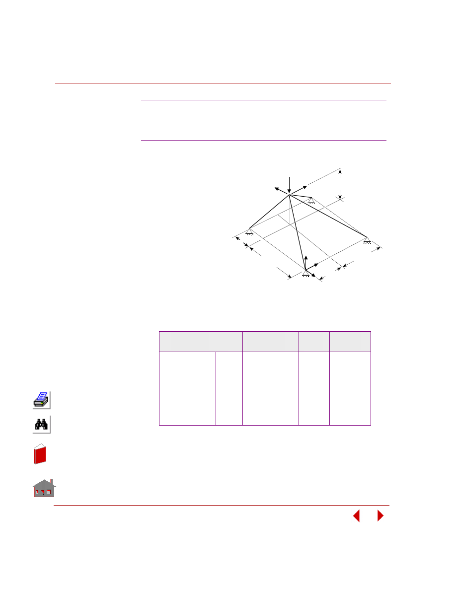
Chapter 5 Additional Problems
5-56
COSMOSM Advanced Modules
KEYWORDS:
Sizing, static analysis,
TRUSS3D, minimum
weight, and stress constraint.
PROBLEM:
Find the minimum weight of
a 4-bar truss subject to
concentrated forces in X, Y,
and Z directions. The
modulus of elasticity is 1E4
ksi and the material density
is 0.10 lb/in
3
. The initial
values and bounds of design
variables, constraints and the
objective function are shown
below.
SUMMARY OF RESULTS:
OPZST5: Minimum Weight of a
4-bar Statically Indeterminate Truss
Subject To Stress Constraints
Optimization Parameters
Initial Value(s)
and Bounds
Final
Value(s)
Tolerance
Design Variables
A1
A2
A3
A4
0.001
≤
1.0
≤
2
0.001
≤
2.0
≤
2
0.001
≤
2.0
≤
2
0.001
≤
1.0
≤
2
0.4708
1.7078
1.2976
0.4873
0.001
0.001
0.001
0.001
Objective Function
Weight
101.879
65.2703
0.001 (Ratio)
Constraints
σ
x
1
σ
x
2
σ
x
3
σ
x
4
-25
≤
-12.165
≤
25
-25
≤
-21.360
≤
25
-25
≤
-16.530
≤
25
-25
≤
-11.89
≤
25
-25.18
-25.163
-25.205
-25.207
0.25
0.25
0.25
0.25
A
1
120"
72"
Y
X
Z
A
2
A
3
A
4
96"
60 K
20 K
10 K
144"
60"
P roble m G e ome t ry
In
de
x
In
de
x
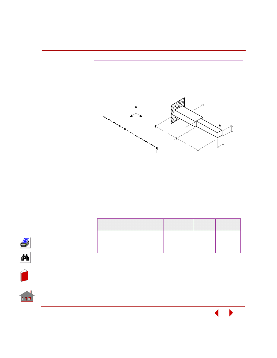
COSMOSM Advanced Modules
5-57
Part 2 OPSTAR / Optimization
KEYWORDS:
Sizing, static analysis, BEAM2D, minimum displacement, and weight constraint.
PROBLEM:
A cantilever beam is subject to a concentrated load at the tip. Find the beam widths
(in each half) maintaining a uniform height of the beam. The beam length is 100 in.,
height is 5 in., modulus of elasticity is 1E07 psi, and material density is 0.1 lb/in
3
.
The initial values and bounds of design variables, constraints and the objective
function are shown below.
SUMMARY OF RESULTS:
OPZST6: Minimum Displacement of a Cantilever
Subject to Weight Constraint – Beam Elements
Optimization Parameters
Initial Value(s)
and Bounds
Final
Value(s)
Tolerance
Design Variables
B1
B2
0.01
≤
1.0
≤
5
0.01
≤
0.25
≤
5
1.4614
0.55234
0.001
0.001
Objective Function
Displacement UY
0.44
0.2640145
0.001 (Ratio)
Constraints
Weight
1
≤
31.25
≤
50
50.344
0.5
B
1
50"
50"
100
5"
B
2
5"
Finit e E le me nt
Me s h
P roble m G e ome t ry
Y
X
Z
In
de
x
In
de
x
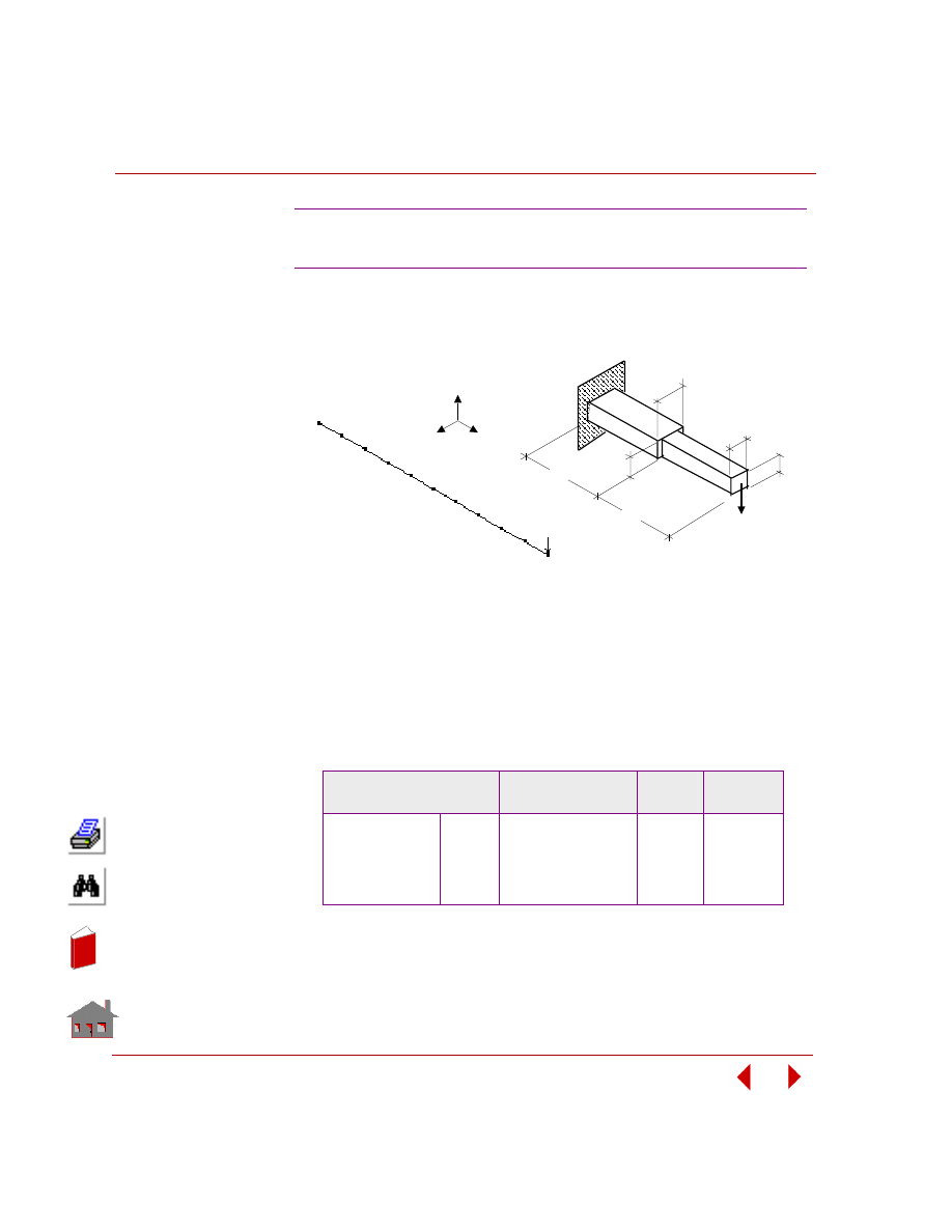
Chapter 5 Additional Problems
5-58
COSMOSM Advanced Modules
KEYWORDS:
Sizing, static analysis, BEAM2D, beam width, minimum weight, and stress
constraint.
PROBLEM:
A cantilever beam is subject to a concentrated load at the tip. Find the beam widths
(in each half) maintaining a uniform height of the beam. The beam length is 100 in.,
height is 5 in., modulus of elasticity is 1E07 psi, and material density is 0.1 lb/in
3
.
The initial values and bounds of design variables, constraints and the objective
function are shown below.
SUMMARY OF RESULTS:
OPZST7: Minimum Weight of a Cantilever
Subject to Stress Constraint – Beam Elements
Optimization Parameters
Initial Value(s)
and Bounds
Final
Value(s)
Tolerance
Design Variables
B1
B2
0.01
≤
3
≤
5
0.01
≤
3
≤
5
0.23833
0.11917
0.001
0.001
Objective Function
Weight
150
8.93745
0.01 (Ratio)
Constraints
σ
x
1
σ
x
2
-10000
≤
800
≤
10000
-10000
≤
400
≤
10000
10,070
10,070
100
100
1
50"
50"
100
B
5"
B
2
5"
Finit e E le me nt
Me s h
P roble m G e ome t ry
Y
X
Z
In
de
x
In
de
x
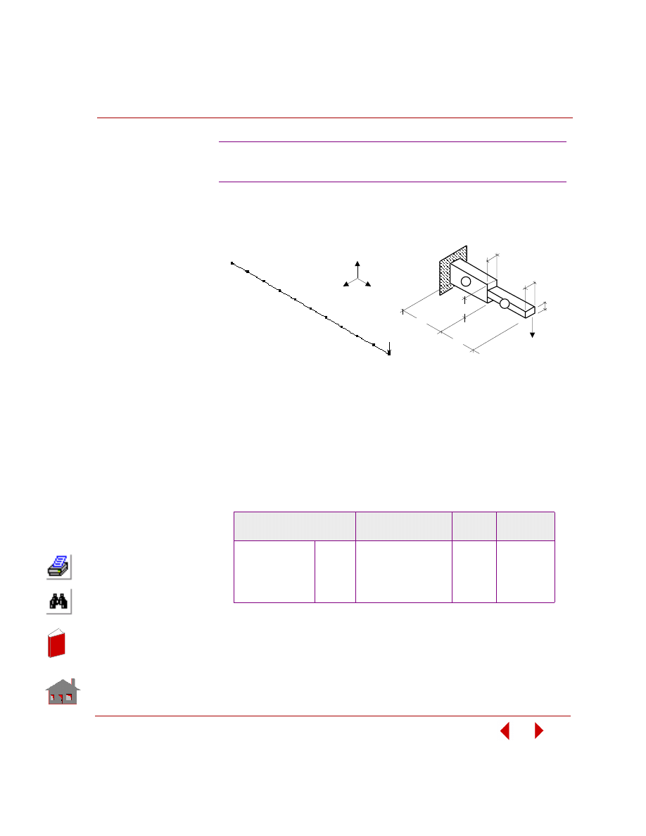
COSMOSM Advanced Modules
5-59
Part 2 OPSTAR / Optimization
KEYWORDS:
Sizing, static analysis, BEAM2D, beam height, minimum weight, and stress
constraint.
PROBLEM:
A cantilever beam is subject to a concentrated load at the tip. Find the beam heights
(in each half) maintaining a uniform width of the beam. The beam length is 100 in.,
width is 5 in, modulus of elasticity is 1E07 psi, and material density is 0.1 lb/in
3
. The
initial values and bounds of design variables, constraints and the objective function
are shown below.
SUMMARY OF RESULTS:
OPZST8: Minimum Weight of a Cantilever
Subject to Stress Constraint – Beam Elements
Optimization Parameters
Initial Value(s)
and Bounds
Final
Value(s)
Tolerance
Design Variables
H1
H2
0.01
≤
2
≤
10
0.01
≤
2
≤
10
1.0916
0.7719
0.01
0.01
Objective Function
Weight
100
46.588
0.001 (Ratio)
Constraints
σ
x
1
σ
x
2
-10000
≤
3000
≤
10000
-10000
≤
1500
≤
10000
10,070
10,070
100
100
5"
5"
H
50"
50"
2
100
1
2
Finit e E le me nt
Me s h
P roble m G e ome t ry
Y
X
Z
H
1
In
de
x
In
de
x
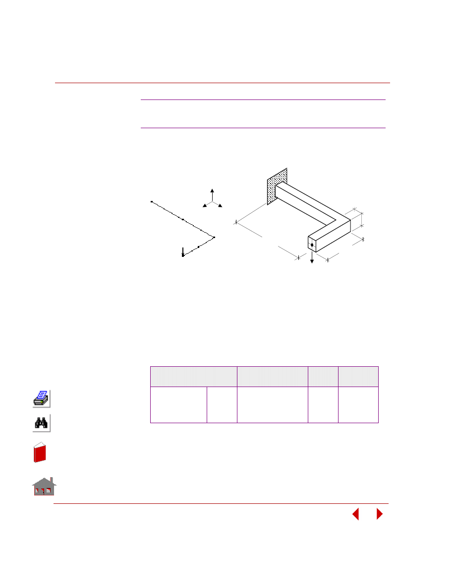
Chapter 5 Additional Problems
5-60
COSMOSM Advanced Modules
KEYWORDS:
Sizing, static analysis, BEAM3D, minimum weight, and displacement constraint.
PROBLEM:
A 3D frame is subject to a concentrated load at the tip. Find the frame height and
width given that width-to-height ratio is equal to the initial ratio. The modulus of
elasticity is 1E07 psi, and material density is 0.1 lb/in
3
. The initial values and bounds
of design variables, constraints and the objective function are shown below.
SUMMARY OF RESULTS:
OPZST9: Minimum Weight of a Frame Subject
to Displacement Constraint – Beam Elements
Optimization Parameters
Initial Value(s)
and Bounds
Final
Value(s)
Tolerance
Design Variables
B
H = 2B
0.1
≤
6
≤
10
—
3.7370
7.4740
0.01
—
Objective Function
Weight
1080
418.96
0.001 (Ratio)
Constraints
UY
-0.10
≤
-0.01536
≤
0.10
-0.1018
0.002
100"
50"
H = 2B
B
Finit e E le me nt
Me s h
P roble m G e ome t ry
Y
X
Z
In
de
x
In
de
x
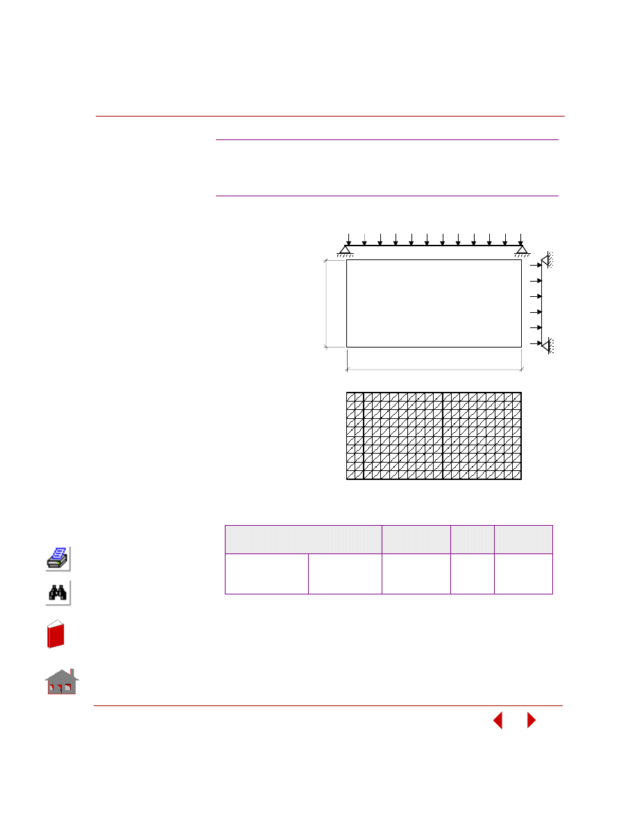
COSMOSM Advanced Modules
5-61
Part 2 OPSTAR / Optimization
KEYWORDS:
Sizing, static
analysis, SHELL3,
bending, minimum
stress, and weight
constraint.
PROBLEM:
Find the thickness of
a 100 x 50 inch plate
subject to pressure of
1 psi. The modulus of
elasticity is 1E07 psi,
Poisson's ratio is 0.3,
and material density
is 0.1 lb/in
3
. The
initial values and
bounds of design
variables, constraints
and the objective
function are shown
below.
SUMMARY OF RESULTS:
OPZST10: Minimum Stress of a Simply
Supported Rectangular Plate Subject
to Weight Constraint – Shell Elements
Optimization Parameters
Initial Value(s)
and Bounds
Final
Value(s)
Tolerance
Design Variables
T (Thickness)
0.01
≤
0.1
≤
1
0.2014
0.001
Objective Function
von Mises stress
132,432
32,649
0.001 (Ratio)
Constraints
Weight 0.01
≤
50
≤
100
100.7
1.0
50"
100"
P = 1 psi
T = Thickness
P roble m G e ome t ry
Finit e E le me nt Me s h
In
de
x
In
de
x
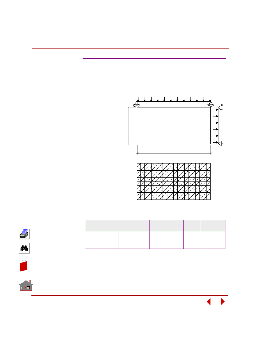
Chapter 5 Additional Problems
5-62
COSMOSM Advanced Modules
KEYWORDS:
Sizing, static
analysis, SHELL3,
minimum weight,
and stress constraint.
PROBLEM:
Find the thickness of
a 100 x 50 inch plate
subject to pressure of
1 psi. The modulus
of elasticity is 1E07
psi, Poisson's ratio is
0.3, and material
density is 0.1 lb/in
3
.
The initial values
and bounds of design
variables, constraints
and the objective
function are shown
below.
SUMMARY OF
RESULTS:
OPZST11: Minimum Weight of a Simply
Supported Rectangular Plate Subject
to Stress Constraint – Shell Elements
Optimization Parameters
Initial Value(s)
and Bounds
Final
Value(s)
Tolerance
Design Variables
T (Thickness)
0.01
≤
2
≤
2
0.87877
0.02
Objective Function
Weight
1000
439.388
0.001 (Ratio)
Constraints
von Mises stress
10
≤
331.08
≤
1700
1714.9
20.0
50"
100"
P = 1 psi
T = Thickness
P roble m G e ome t ry
Finit e E le me nt Me s h
In
de
x
In
de
x
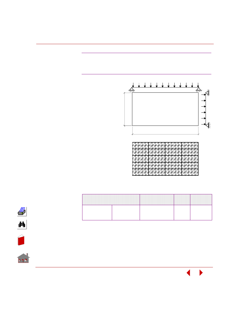
COSMOSM Advanced Modules
5-63
Part 2 OPSTAR / Optimization
KEYWORDS:
Sizing, static analysis,
SHELL3, bending,
minimum weight, and
displacement
constraint.
PROBLEM:
Find the thickness of a
100 x 50 inch plate
subject to pressure of
1 psi. The modulus of
elasticity is 1E07 psi,
Poisson's ratio is 0.3,
and material density is
0.1 lb/in
3
. The initial
values and bounds of
design variables,
constraints and the
objective function are
shown below.
SUMMARY OF RESULTS:
OPZST12: Minimum Weight of a Simply
Supported Rectangular Plate Subject to
Displacement Constraint – Shell Elements
Optimization Parameters
Initial Value(s)
and Bounds
Final
Value(s)
Tolerance
Design Variables
T (Thickness)
0.01
≤
2
≤
5
0.87757
0.01
Objective Function
Weight
1000
438.78
0.001 (Ratio)
Constraints
Displacement UZ
-0.10
≤
-0.0086
≤
0.10
-0.1017
0.002
50"
100"
P = 1 psi
T = Thickness
P roble m G e ome t ry
Finit e E le me nt Me s h
In
de
x
In
de
x
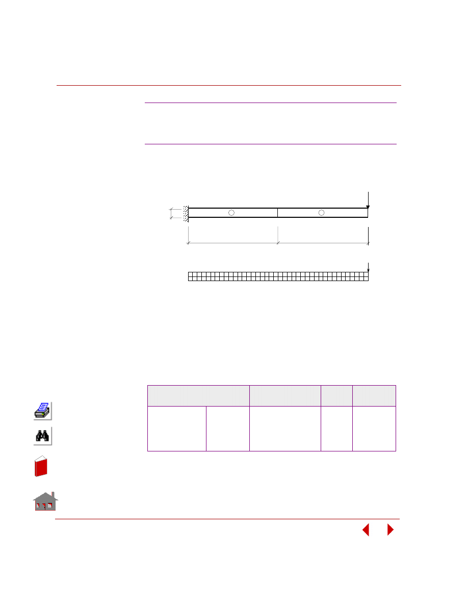
Chapter 5 Additional Problems
5-64
COSMOSM Advanced Modules
KEYWORDS:
Sizing, static analysis, 8-node PLANE2D, minimum weight, and stress constraint.
PROBLEM:
Find the cantilever plate thickness for each half. The cantilever length is 100 in.,
height is 5 in., modulus of elasticity is 1E07 psi, Poisson's ratio is 0, and material
density is 0.1 lb/in
3
. The initial values and bounds of design variables, constraints
and the objective function are shown below.
SUMMARY OF RESULTS:
OPZST13: Minimum Weight of a Cantilever
Plate Subject to Stress Constraint –
Quadrilateral Continuum Elements
Optimization Parameters
Initial Value(s)
and Bounds
Final
Value(s)
Tolerance
Design Variables
B1
B2
0.01
≤
2
≤
2
0.01
≤
2
≤
2
0.23850
0.11628
0.001
0.001
Objective Function
Weight
100
8.86944
0.001 (Ratio)
Constraints
von Mises 1
von Mises 2
-10000
≤
1200
≤
10,000
-10000
≤
600
≤
10,000
10,070
10,069
100
100
100 lbs
50"
5"
50"
P roble m G e ome t ry
Finit e E le me nt Me s h
1
2
In
de
x
In
de
x
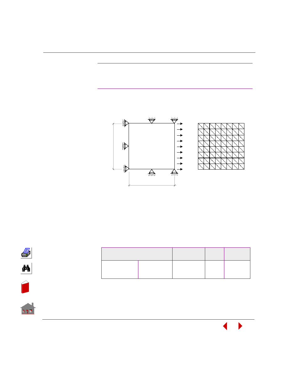
COSMOSM Advanced Modules
5-65
Part 2 OPSTAR / Optimization
KEYWORDS:
Sizing, static analysis, 3-node TRIANG, minimum weight, and displacement
constraint.
PROBLEM:
Find the plate thickness. The plate length is 1 inch, height is 1 inch, modulus of
elasticity is 5 psi, and Poisson's ratio is 0. The initial values and bounds of design
variables, constraints and the objective function are shown below.
SUMMARY OF RESULTS:
OPZST14: Minimum Volume of a Plate
Subject to Displacement Constraint –
Triangular Continuum Elements
Optimization Parameters
Initial Value(s)
and Bounds
Final
Value(s)
Tolerance
Design Variables
T (Thickness)
0.1
≤
1
≤
2
0.50025
0.01
Objective Function
Volume
1.0
0.50025
0.001 (Ratio)
Constraints
Displacement UX
0.01
≤
0.2
≤
0.4
0.3998
0.001
1"
1"
1 ps
i
P roble m G e ome t ry
Finit e E le me nt Me s h
T = Thickness
In
de
x
In
de
x
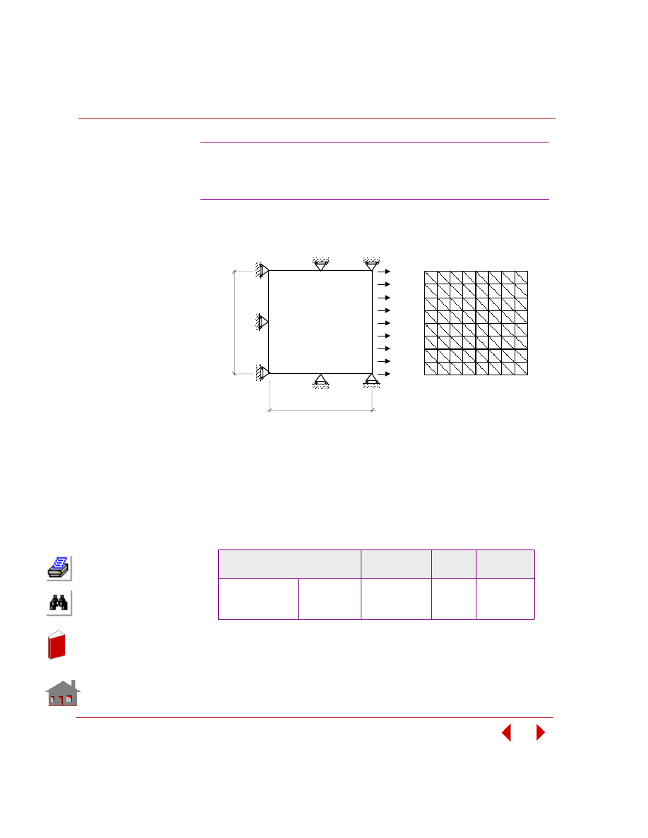
Chapter 5 Additional Problems
5-66
COSMOSM Advanced Modules
KEYWORDS:
Sizing, static analysis, 3-node TRIANG, minimum weight, and stress constraint.
PROBLEM:
Find the plate thickness. The plate length is 1 inch, height is 1 inch, modulus of
elasticity is 5 psi, and Poisson's ratio is 0. The initial values and bounds of design
variables, constraints and the objective function are shown below.
SUMMARY OF RESULTS:
OPZST15: Minimum Volume of a Plate
Subject to Stress Constraint –
Triangular Continuum Elements
Optimization Parameters
Initial Value(s)
and Bounds
Final
Value(s)
Tolerance
Design Variables
T (Thickness)
0.1
≤
1
≤
2
0.499
0.01
Objective Function
Volume
1.0
0.499
0.001 (Ratio)
Constraints
Stress
σx
0.1
≤
1.0
≤
2.0
2.004
0.01
1"
1"
1 ps
i
P roble m G e ome t ry
Finit e E le me nt Me s h
T = Thickness
In
de
x
In
de
x
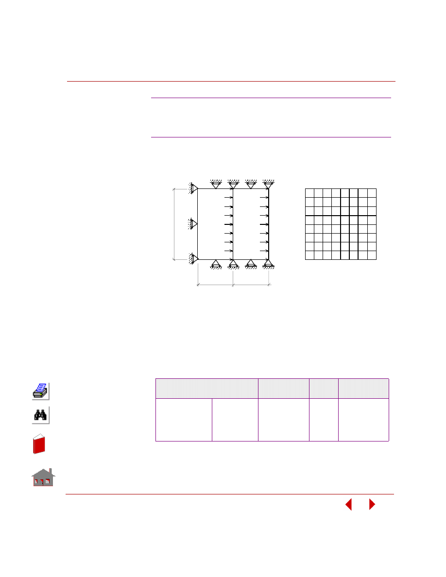
COSMOSM Advanced Modules
5-67
Part 2 OPSTAR / Optimization
KEYWORDS:
Sizing, static analysis, 8-node PLANE2D, minimum volume, and stress constraint.
PROBLEM:
Find the plate thickness for each half. The plate length is 1 inch, height is 1 inch,
modulus of elasticity is 5 psi, and Poisson's ratio is 0. The initial values and bounds
of design variables, constraints and the objective function are shown below.
SUMMARY OF RESULTS:
OPZST16: Minimum Volume of a Plate
Subject to Stress Constraint –
Quadrilateral Continuum Elements
Optimization Parameters
Initial Value(s)
and Bounds
Final
Value(s)
Tolerance
Design Variables
T1 (Thickness)
T2 (Thickness)
0.1
≤
2
≤
2
0.1
≤
1
≤
2
1.0034
0.499
0.01
0.01
Objective Function
Volume
1.5
0.7512
0.001 (Ratio)
Constraints
Stress
σ
x
1
Stress
σ
x
2
-2
≤
1.0
≤
2
-2
≤
1.0
≤
2
1.9932
2.004
0.01
0.01
1"
0.5"
1 ps
i
0.5"
Thickness
T
1
Thickness
T
2
P roble m G e ome t ry
Finit e E le me nt Me s h
In
de
x
In
de
x
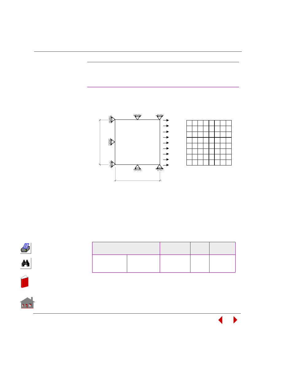
Chapter 5 Additional Problems
5-68
COSMOSM Advanced Modules
KEYWORDS:
Sizing, static analysis, 4-node PLANE2D, minimum volume, and stress constraint.
PROBLEM:
Find the plate thickness. The plate length is 1 inch, height is 1 inch, modulus of
elasticity is 5 psi, and Poisson's ratio is 0. The initial values and bounds of design
variables, constraints and the objective function are shown below.
SUMMARY OF RESULTS:
OPZST17: Minimum Volume of a Plate
Subject to Stress Constraint –
Quadrilateral Continuum Elements
Optimization Parameters
Initial Value(s)
and Bounds
Final
Value(s)
Tolerance
Design Variables
T (Thickness)
0.1
≤
1
≤
1
0.50126
0.01
Objective Function
Volume
1.0
0.50126
0.001 (Ratio)
Constraints
von Mises stress
0
≤
1.0
≤
2.0
1.995
0.001
1"
1"
1 ps
i
P roble m G e ome t ry
Finit e E le me nt Me s h
T = Thickness
In
de
x
In
de
x
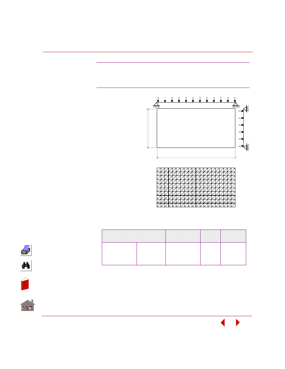
COSMOSM Advanced Modules
5-69
Part 2 OPSTAR / Optimization
KEYWORDS:
Sizing, static analysis,
SHELL3, bending,
minimum weight, and
effective strain
constraint.
PROBLEM:
Find the thickness of a
100 x 50 inch plate
subject to pressure of
1 psi. The modulus of
elasticity is 1E07 psi,
Poisson's ratio is 0.3,
and material density is
0.1 lb/in
3
. The initial
values and bounds of
design variables,
constraints and the
objective function are
shown below.
SUMMARY OF RESULTS:
OPZST18: Minimum Weight of a Simply
Supported Rectangular Plate Subject to
Effective Strain Constraint – Shell Elements
Optimization Parameters
Initial Value(s)
and Bounds
Final
Value(s)
Tolerance
Design Variables
T (Thickness)
0.01
≤
2
≤
5
0.87699
0.01
Objective Function
Weight
1000
438.495
0.001 (Ratio)
Constraints
Effective Strain
2.0E-5
≤
2.47E-5
≤
1.28E-4
1.287E-4
1.08E-6
50"
100"
P = 1 psi
T = Thickness
P roble m G e ome t ry
Finit e E le me nt Me s h
In
de
x
In
de
x
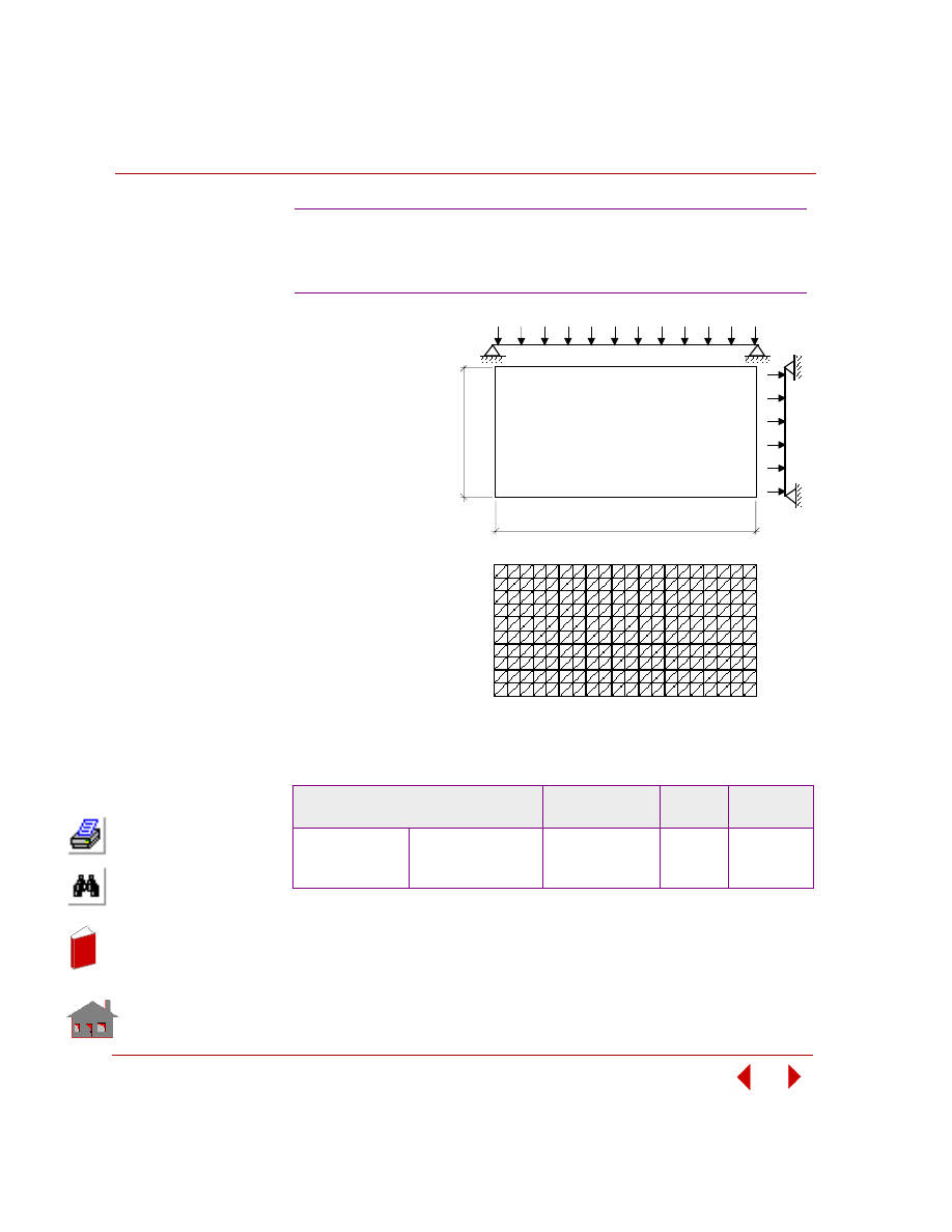
Chapter 5 Additional Problems
5-70
COSMOSM Advanced Modules
KEYWORDS:
Sizing, static analysis,
SHELL3, bending,
minimum weight, and
strain energy density
constraint.
PROBLEM:
Find the thickness of a
100 x 50 inch plate
subject to pressure of
1 psi. The modulus of
elasticity is 1E07 psi,
Poisson's ratio is 0.3,
and material density
is 0.1 lb/in
3
. The
initial values and
bounds of design
variables, constraints
and the objective
function are shown
below.
SUMMARY OF RESULTS:
OPZST19: Minimum Weight of a Simply
Supported Rectangular Plate Subject to Strain
Energy Density Constraint – Shell Elements
Optimization Parameters
Initial Value(s)
and Bounds
Final
Value(s)
Tolerance
Design Variables
T (Thickness)
0.01
≤
2
≤
5
0.8771
0.01
Objective Function
Weight
1000
438.550
0.001 (Ratio)
Constraints
Strain Energy Density
0
≤
0.0022
≤
0.059
0.05941
0.00059
50"
100"
P = 1 psi
T = Thickness
P roble m G e ome t ry
Finit e E le me nt Me s h
In
de
x
In
de
x
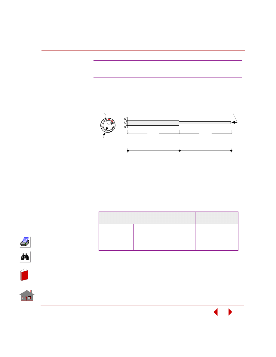
COSMOSM Advanced Modules
5-71
Part 2 OPSTAR / Optimization
KEYWORDS:
Sizing, static analysis, PIPE, radius of cross-section, minimum volume, and stress
constraint.
PROBLEM:
A cantilever pipe is subject to a concentrated load at the tip. Find the pipe radii (in
each half). The cantilever length is 100 inches, modules of elasticity is 1 x 10
7
psi,
and Poisson's ratio is 0.30. The initial values and bounds of design variables,
objectives function and constraints are shown below.
SUMMARY OF RESULTS:
OPZST20: Minimum Volume of a Cantilever Pipe
Subject to Stress Constraint – Pipe Radius
Optimization Parameters
Initial Value(s)
and Bounds
Final
Value(s)
Tolerance
Design Variables
RAVE1
RAVE2
0.5
≤
1.6
≤
2
0.5
≤
1.6
≤
2
1.2994
0.9650
0.015
0.015
Objective Function
Volume
231.6925
158.21
0.01 (Ratio)
Constraints
σ
x
1
σ
x
2
-10,000
≤
6,302
≤
10,000
-10,000
≤
3,151
≤
10,000
10,100
10,140
200
200
100
Radius
P roble m Ge ome try
Finite E le me nt Me sh
Thickness
50"
Average Radius 1
Average Radius 2
50"
In
de
x
In
de
x
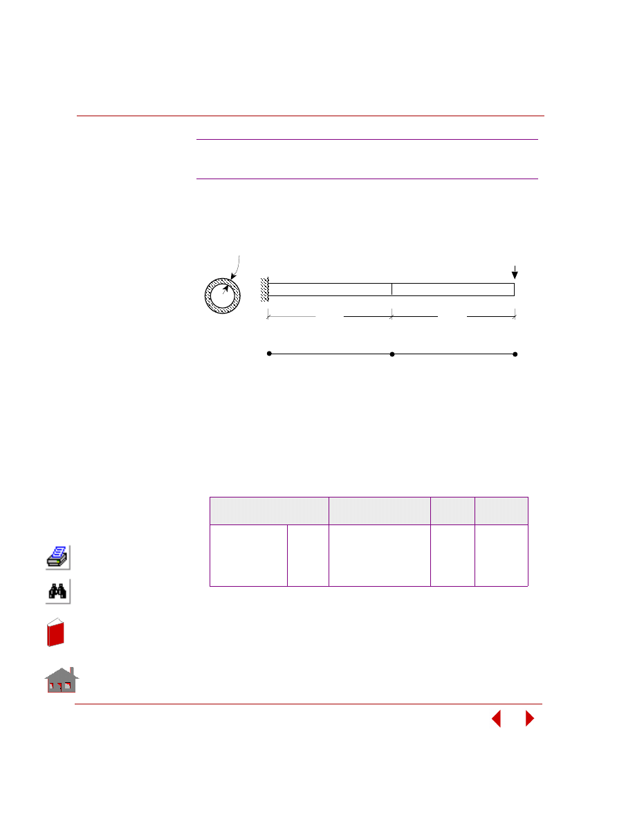
Chapter 5 Additional Problems
5-72
COSMOSM Advanced Modules
KEYWORDS:
Sizing, static analysis, PIPE, thickness of cross section, minimum volume, and stress
constraint.
PROBLEM:
A cantilever pipe is subject to a concentrated load at the tip. Find the pipe thickness
(in each half). The cantilever length is 100 inches, modules of elasticity is 1 x 10
7
psi, and Poisson's ratio is 0.30. The initial values and bounds of design variables,
objectives function and constraints are shown below.
SUMMARY OF RESULTS:
OPZST21: Minimum Volume of a Cantilever Pipe
Subject to Stress Constraint – Pipe Thickness
Optimization Parameters
Initial Value(s)
and Bounds
Final
Value(s)
Tolerance
Design Variables
T1
T2
0.01
≤
0.50
≤
0.5
0.01
≤
0.25
≤
0.5
0.1644
0.07497
0.005
0.005
Objective Function
Volume
304.3418
107.68
0.01 (Ratio)
Constraints
σ
x
1
σ
x
2
-10,000
≤
4,701
≤
10,000
-10,000
≤
3,643
≤
10,000
10,149
10,170
200
200
50"
T
T
50"
100
Thickness
P roble m Ge ome try
Finite E le me nt Me sh
2
1
In
de
x
In
de
x
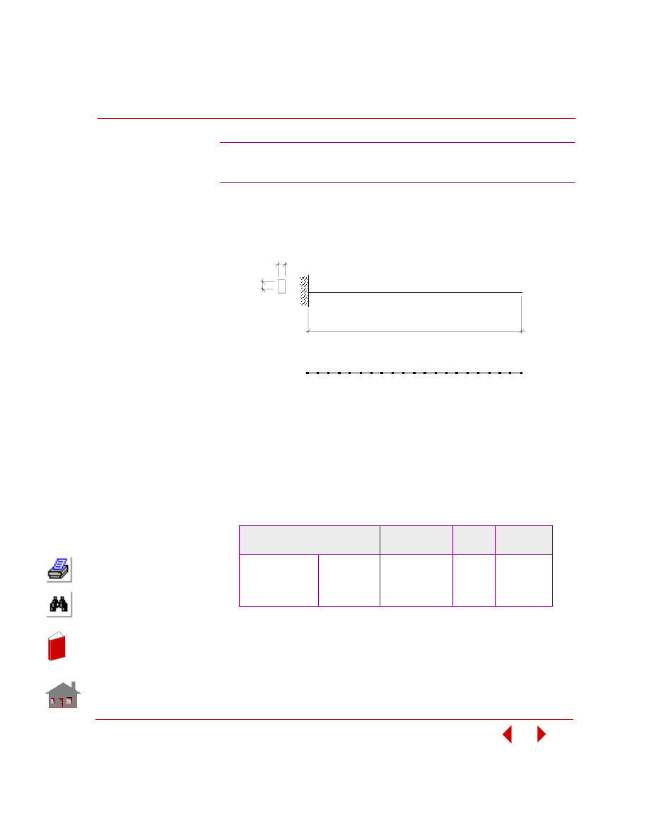
COSMOSM Advanced Modules
5-73
Part 2 OPSTAR / Optimization
KEYWORDS:
Sizing, frequency analysis, BEAM2D, minimum weight, and fundamental
frequency constraint.
PROBLEM:
Find the height of a cantilever. The beam's length is 100 inches, width is 1 inch,
modulus of elasticity is 1 x 10
7
psi and material density is 0.10 lb/in
3
. The initial
values and bounds of design variables, constraints and the objective function are
shown below.
SUMMARY OF RESULTS:
OPZFQ1: Minimum Weight of a Cantilever Subject
to Frequency Constraint – Beam Elements
Optimization Parameters
Initial Value(s)
and Bounds
Final
Value(s)
Tolerance
Design Variables
H (Height)
0.1
≤
10
≤
20
4.9109
0.01
Objective Function
Weight
100
49.109
0.01 (Ratio)
Constraints
Fundamental
frequency
0.8
≤
1.6135
≤
4
0.7924
0.01
E = 10 psi
100"
7
Cros s
S e c t ion
1"
H
P roble m G e ome t ry
Finit e E le me nt Me s h
In
de
x
In
de
x
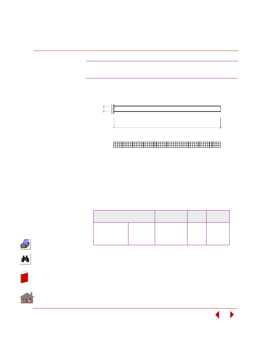
Chapter 5 Additional Problems
5-74
COSMOSM Advanced Modules
KEYWORDS:
Sizing, frequency analysis, SHELL4, minimum weight, and frequency constraint.
PROBLEM:
Find the cantilever plate thickness. The cantilever length is 100 in, height is 5 in,
modulus of elasticity is 1 x 10
7
psi, and material density is 0.1 lb/in
3
. The initial
values and bounds of design variables, constraints and the objective function are
shown below.
SUMMARY OF RESULTS:
OPZFQ2: Minimum Weight of a Cantilever Subject
to Frequency Constraint – Shell Elements
Optimization Parameters
Initial Value(s)
and Bounds
Final
Value(s)
Tolerance
Design Variables
DV1
0.1
≤
2
≤
3
0.18494
0.001
Objective Function
Weight
100
9.24676
0.01 (Ratio)
Constraints
Fundamental
frequency
0.03
≤
0.3243
≤
1
0.029989
0.0001
100"
5"
P roble m G e ome t ry
Finit e E le me nt Me s h
In
de
x
In
de
x
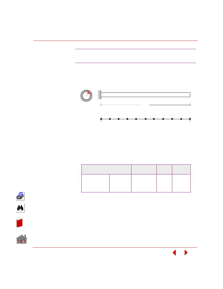
COSMOSM Advanced Modules
5-75
Part 2 OPSTAR / Optimization
KEYWORDS:
Sizing, frequency analysis, PIPE, radius of cross-section, minimum weight, and
frequency constraint.
PROBLEM:
Find the pipe radius. The cantilever length is 100 in., modulus of elasticity is 1 x 10
7
psi, and material density is 0.1 lb/in
3
. The initial values and bounds of design
variables, constraints and the objective function are shown below.
SUMMARY OF RESULTS:
OPZFQ3: Minimum Weight of a Pipe Cantilever
Subject to Frequency Constraint – Pipe Elements
Optimization Parameters
Initial Value(s)
and Bounds
Final
Value(s)
Tolerance
Design Variables
R
0.1
≤
1.5
≤
2
0.57467
0.019
Objective Function
Weight
21.59846
7.063443
0.01 (Ratio)
Constraints
Fundamental
frequency
0.2
≤
0.5432
≤
2
0.18381
0.018
100"
P roble m Ge ome try
Finite E le me nt Me sh
R
In
de
x
In
de
x
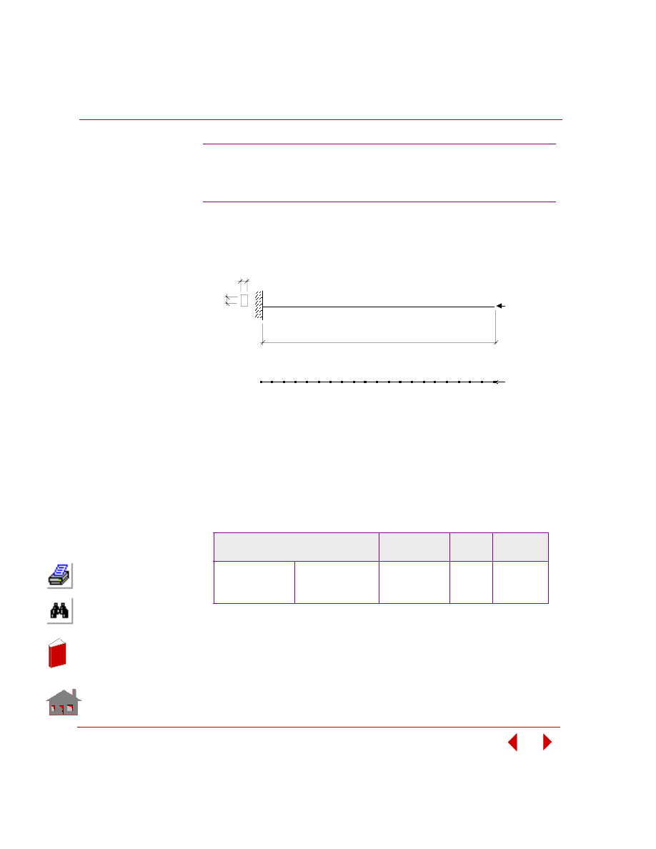
Chapter 5 Additional Problems
5-76
COSMOSM Advanced Modules
KEYWORDS:
Sizing, buckling analysis, BEAM2D, minimum weight, and buckling load factor
constraint.
PROBLEM:
Find the height of a cantilever beam subject to a concentrated compressive force of
1000 lb The beam's length is 100 in, width is 5 in, modulus of elasticity is 1 x 10
7
psi and material density is 0.10 lb/in
3
. The initial values and bounds of design
variables, constraints and the objective function are shown below.
SUMMARY OF RESULTS:
OPZBK1: Minimum Weight of a Cantilever
Subject to Buckling Load Factor
Constraint – Beam Elements
Optimization Parameters
Initial Value(s)
and Bounds
Final
Value(s)
Tolerance
Design Variables
H (Height)
0.1
≤
5
≤
10
2.101
0.001
Objective Function
Weight
50
21.007
0.01 (Ratio)
Constraints
Buckling load factor
2
≤
25.702
≤
50
1.9060
0.1
E = 10 psi
F = 1,000 lb
100"
7
P roble m Ge ome try
Finite E le me nt Me sh
Cros s
S e c t ion
1"
H
In
de
x
In
de
x
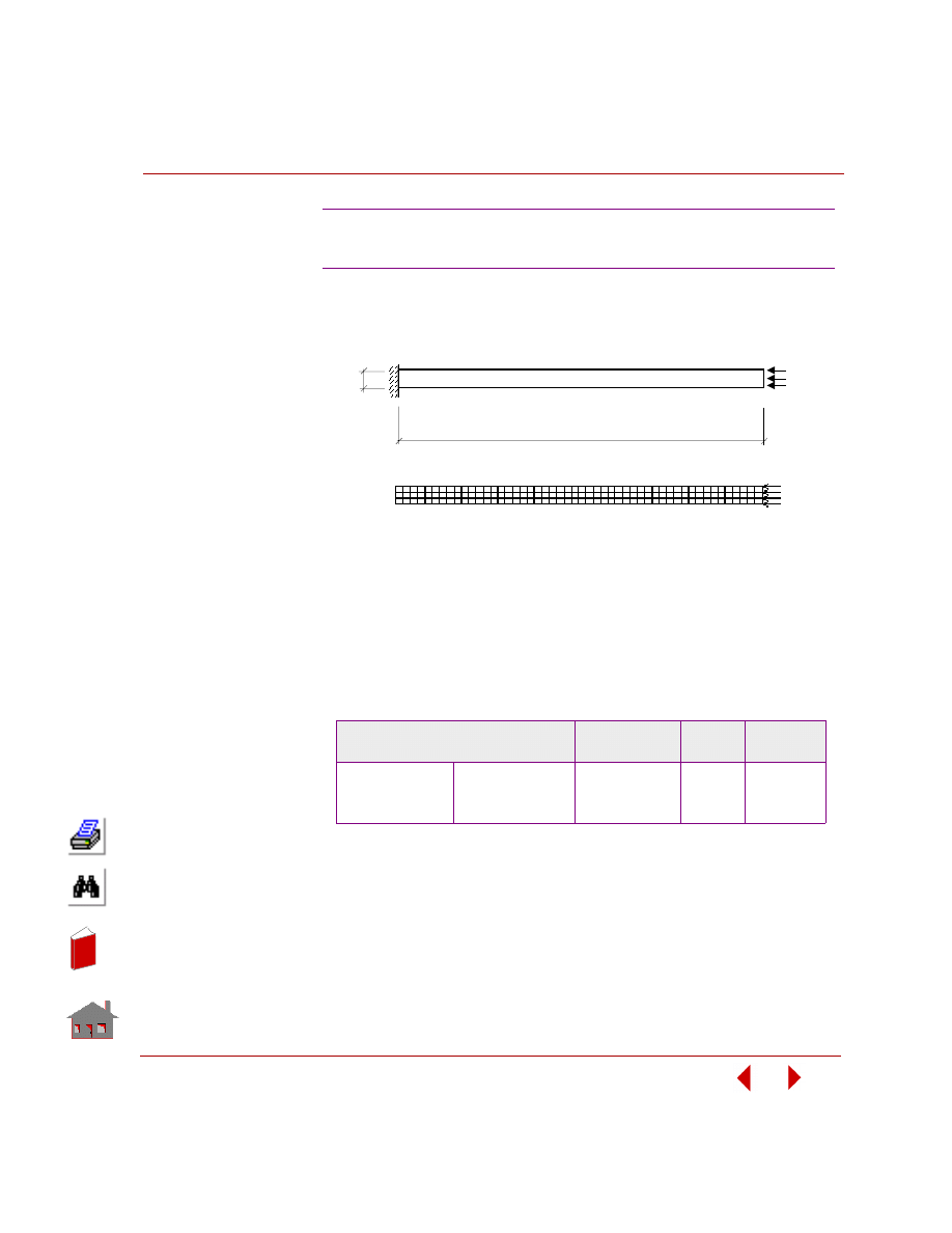
COSMOSM Advanced Modules
5-77
Part 2 OPSTAR / Optimization
KEYWORDS:
Sizing, buckling analysis, SHELL4, and minimum weight, buckling constraint.
PROBLEM:
Find the cantilever plate thickness. The cantilever length is 100 in, height is 5 in,
modulus of elasticity is 1 x 10
7
psi, and material density is 0.1 lb/in
3
. The initial
values and bounds of design variables, constraints and the objective function are
shown below.
SUMMARY OF RESULTS:
OPZBK2: Minimum Weight of a Cantilever
Subject to Buckling Constraint – Shell Elements
Optimization Parameters
Initial Value(s)
and Bounds
Final
Value(s)
Tolerance
Design Variables
T (Thickness)
0.1
≤
2
≤
3
1.2279
0.001
Objective Function
Weight
100
61.393
0.01 (Ratio)
Constraints
Buckling load factor
2
≤
8.2604
≤
50
1.9115
0.01
250
lbs/
Node
100"
5"
P roble m G e ome t ry
Finit e E le me nt Me s h
In
de
x
In
de
x
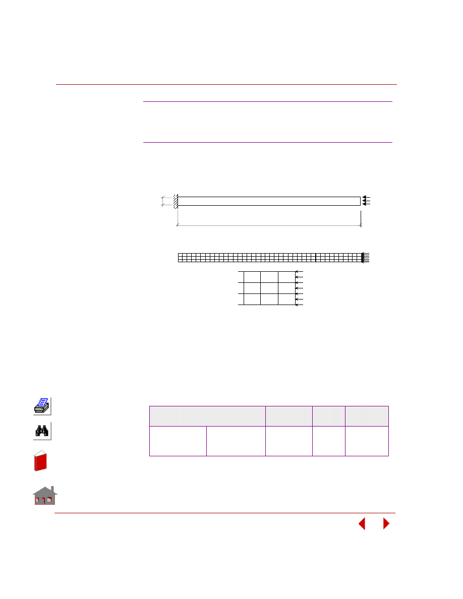
Chapter 5 Additional Problems
5-78
COSMOSM Advanced Modules
KEYWORDS:
Sizing, buckling analysis, 8-node PLANE2D, minimum weight, and buckling
constraint.
PROBLEM:
Find the cantilever plate thickness. The cantilever length is 100 inches, height is 5
inches, modulus of elasticity is 1 x 10
7
psi, and material density is 0.1 psi. The initial
values and bounds of design variables, constraints and the objective function are
shown below.
SUMMARY OF RESULTS:
OPZBK3: Minimum Weight of a Cantilever
Plate Subject to Buckling Constraint –
Quadrilateral Continuum Elements
Optimization Parameters
Initial Value(s)
and Bounds
Final
Value(s)
Tolerance
Design Variables
T (Thickness)
0.1
≤
1
≤
2
0.13
0.001
Objective Function
Weight
50
6.50
0.001 (Ratio)
Constraints
Buckling load factor
2
≤
14.66
≤
50
1.906
0.1
250
lbs/
Node
100"
5"
P roble m Ge ome try
Finite E le me nt Me sh
In
de
x
In
de
x
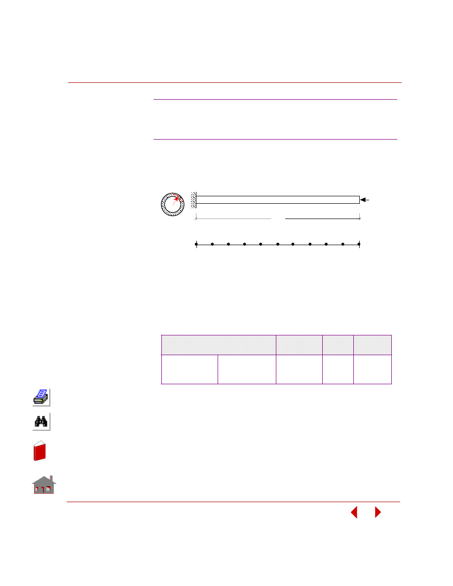
COSMOSM Advanced Modules
5-79
Part 2 OPSTAR / Optimization
KEYWORDS:
Sizing, buckling analysis, PIPE, radius of cross-section, minimum weight, and
linearized buckling constraint.
PROBLEM:
Find the pipe radius. The cantilever length is 100 in, modulus of elasticity is 1 x 10
7
psi, and material density is 0.1 lb/in
3
. The initial values and bounds of design
variables, constraints and the objective function are shown below.
SUMMARY OF RESULTS:
OPZBK4: Minimum Weight of a Pipe
Cantilever Subject to Buckling Load
Constraint – Pipe Elements
Optimization Parameters
Initial Value(s)
and Bounds
Final
Value(s)
Tolerance
Design Variables
R
0.1
≤
1.5
≤
2
1.1242
0.019
Objective Function
Weight
21.598
15.696
0.01 (Ratio)
Constraints
Buckling load factor
2
≤
5.0732
≤
6
1.9624
0.04
100"
1,000 lbs
R
P roble m Ge ome try
Finite E le me nt Me sh
In
de
x
In
de
x
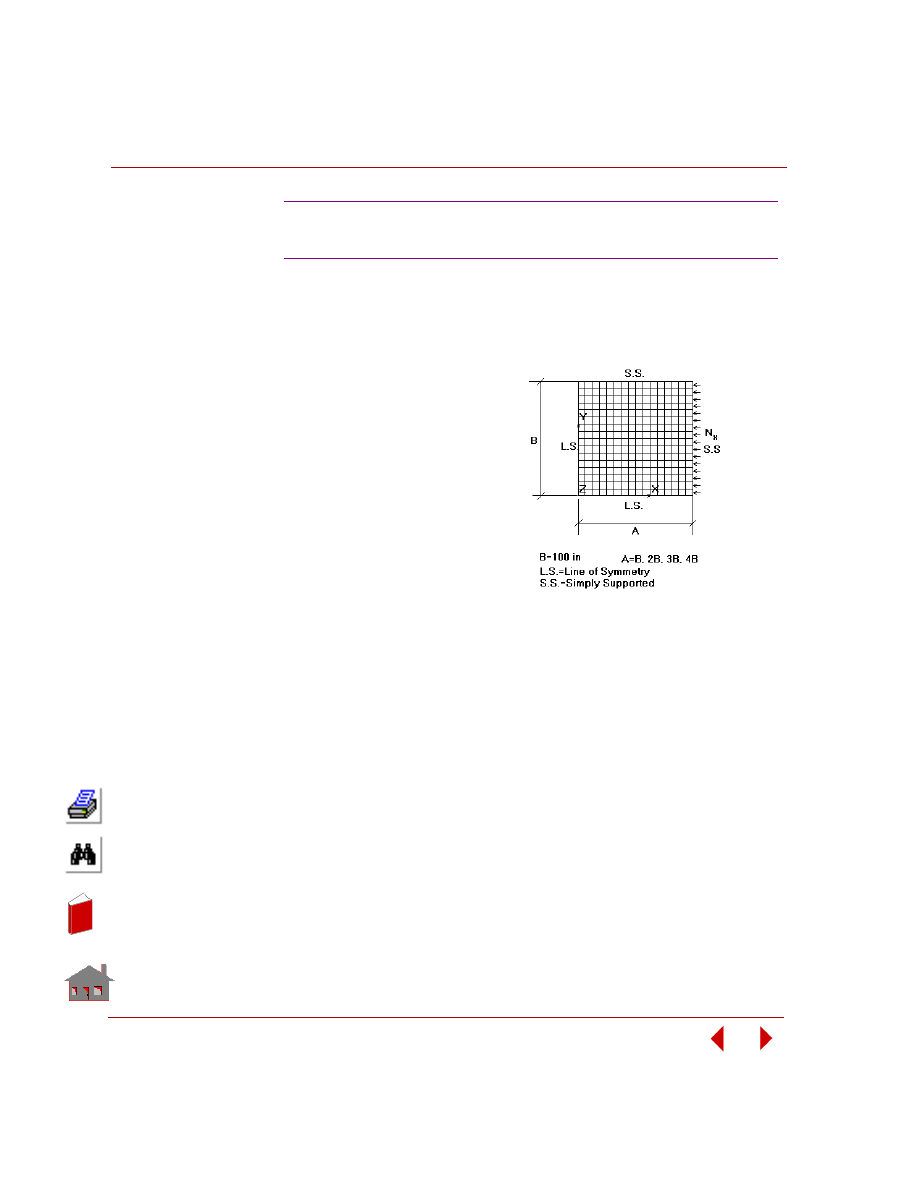
Chapter 5 Additional Problems
5-80
COSMOSM Advanced Modules
KEYWORDS:
Buckling analysis, SHELL4L elements, sizing optimization (ply orientation),
maximum buckling load factor
λ
cr
.
PROBLEM:
Find the ply orientation
θ of a
8-layer [
θ / -θ / θ / - θ]
s
Graphite-Epoxy laminated
composite plate which is
subject to a uniaxial edge
pressure loading 1 psi. The
total thickness of 8 plies is 1
inch. The material constants
are given as: modulus of
elasticity in the first material
direction E
x
= 26.27E6 psi,
modulus of elasticity in the
second material direction E
y
=
1.49E6 psi, Poisson’s ratio
υ =
0.28, shear modulus in the
material first and second plane G
xy
= 1.04E6 psi, tensile and compressive strengths
in the first material direction F
1T
= F
1C
= 2.17E5 psi, tensile and compressive
strengths in the second material direction F
2T
= 5.81E3 psi and F
2C
= 3.57E4 psi,
shear strength in the material first and second plane F
12
= 9.87E3 psi. Four cases are
studied in which the aspect ratios of the dimension A to B are equal to 1, 2, 3, and 4.
The input data regarding optimization as well as the converged results are listed in
the following table. Note that the optimum design is achieved without applying any
constraint.
OPZBK5: Maximum Buckling Load
Design of a Graphite-epoxy Laminate
Initial Problem Geometry and Finite Element Mesh
In
de
x
In
de
x
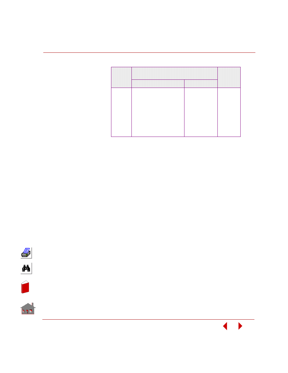
COSMOSM Advanced Modules
5-81
Part 2 OPSTAR / Optimization
SUMMARY OF RESULTS:
A/B
Optimization Parameters
Design Variable,
θ −
Objective Function,
λ
cr
Tolerance
Initial Value(s) and Bounds
Final Value(s)
1
1.E-16 < 30 < 90
45.146
0.9
860.96
948.96
0.01 (ratio)
2
1.E-16 < 30 < 90
41.986
0.9
846.81
1193.0
0.01 (ratio)
3
1.E-16 < 30 < 90
44.985
0.9
965.58
1062.6
0.01 (ratio)
4
1.E-16 < 30 < 90
46.768
0.9
888.42
1126.1
0.01 (ratio)
In
de
x
In
de
x
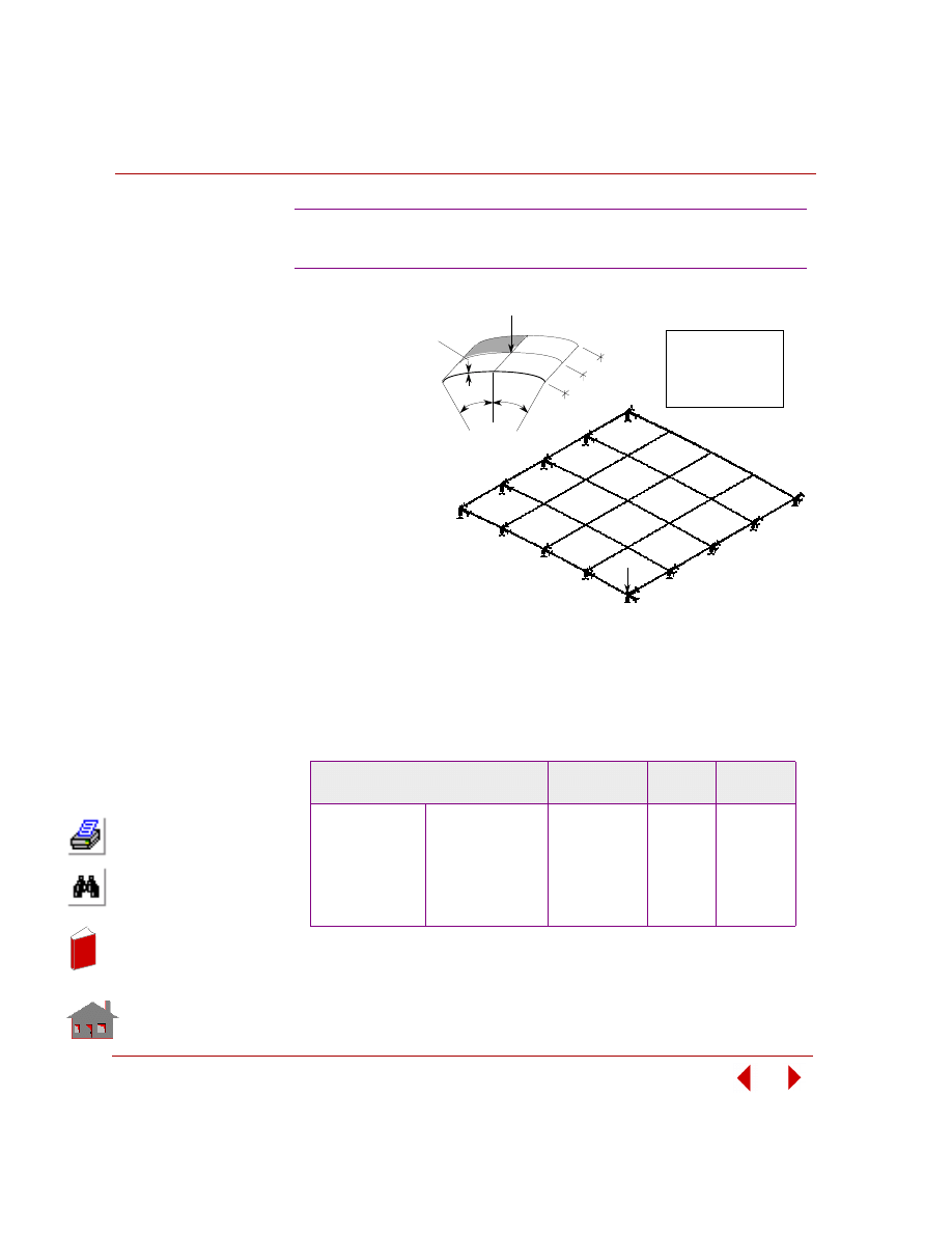
Chapter 5 Additional Problems
5-82
COSMOSM Advanced Modules
KEYWORDS:
Sizing, nonlinear
analysis,
linearized
buckling, snap-
through/snap-
back, arc-length,
limit point,
SHELL4,
minimum
volume, and
user-defined
constraint.
PROBLEM:
Find the thickness
of a thin
cylindrical shell.
The curved edges of the shell are free while the straight edges are hinged and
immovable. The modulus of elasticity is 3102.75 N/mm
2
and Poisson's ratio is 0.3.
The initial values and bounds of design variables, constraints and objective function
are shown below.
SUMMARY OF RESULTS:
OPZNB1: Snap Buckling of a Thin Hinged
Cylindrical Shell Under a Central Point Load
Optimization Parameters
Initial Value(s)
and Bounds
Final
Value(s)
Tolerance
Design Variables
Thickness
5
≤
10
≤
10
5.7611
0.10
Objective Function
Volume
6.451412 x 10
5
3.7167E5
0.01 (Ratio)
Constraints
Limit Point Load
Factor or Linearized
Buckling Load
Factor (user-
defined)
50
≤
588.39
≤
10,000
49.151
1.0
E
ν
R
b
θ
= 3102.75 N/mm
= 0.30
= 2540 mm
= 254 mm
= 0.10 Rad
2
P = 1.0
Thickness
b
b
R
θ
θ
Finite Ele me nt
Me sh
In
de
x
In
de
x
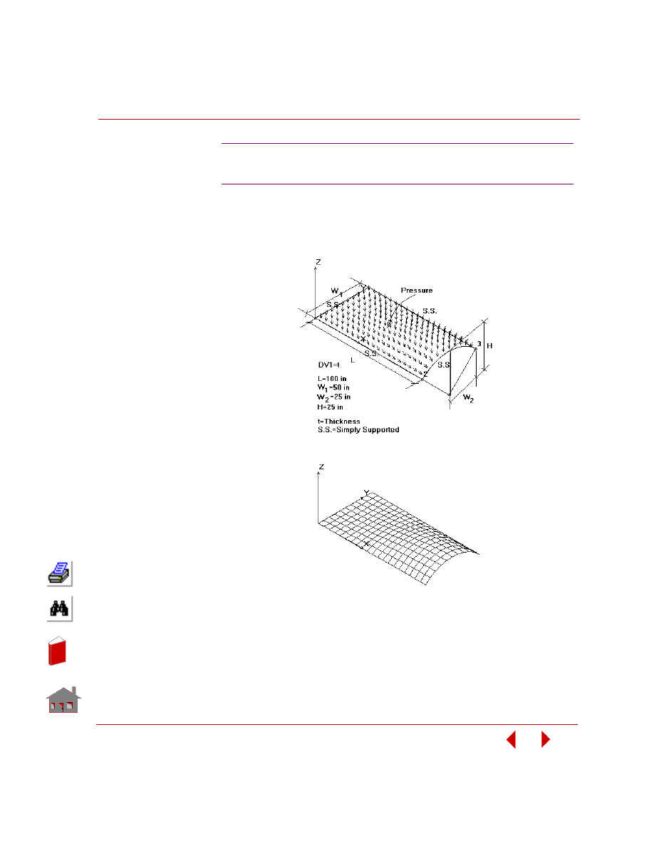
COSMOSM Advanced Modules
5-83
Part 2 OPSTAR / Optimization
KEYWORDS:
Frequency analysis, post-dynamic analysis (time history analysis), dynamic stress
analysis, SHELL4 elements, sizing optimization, multidisciplinary optimization,
minimum strain design, frequency and mass constraints.
Initial Problem Geometry
Initial Finite Element Mesh
OPZFDS1: Modal Time History Analysis
of a Simply Supported Shell Structure
In
de
x
In
de
x
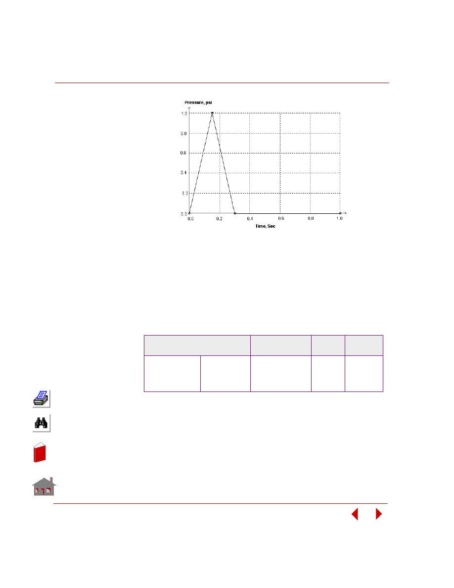
Chapter 5 Additional Problems
5-84
COSMOSM Advanced Modules
Pressure Loading versus Time Curve
PROBLEM:
Find the thickness t of a simply supported shell structure which is subject to an
impulsive pressure loading 1 psi. The material constants of the shell are given as:
Young’s modulus E = 1E7 psi, Poisson’s ratio
υ = 0.3, and Density ρ = 0.1 lb*sec
2
/
in
4
. The input data regarding optimization as well as the converged results are listed
in the following table. Note that the objective function, effective strain, is defined as
the extreme value within the desired range of time (0.0 - 0.6 sec).
SUMMARY OF RESULTS:
Optimization Parameters
Initial Value(s)
and Bounds
Final
Value(s)
Tolerance
Design Variables
DV1
0.01
≤
0.1
≤
1
0.1927
0.001
Objective Function
Effective Strain
5.6057E-4
2.7323E-4
0.01 (Ratio)
Constraints
Frequency (1st)
Mass
1
≤
31560
≤
10
0.01
≤
52.255
≤
100.
3.9598
100.70
0.09
1.0
In
de
x
In
de
x

COSMOSM Advanced Modules
5-85
Dominantly Shape
Sensitivity Problems
In
de
x
In
de
x
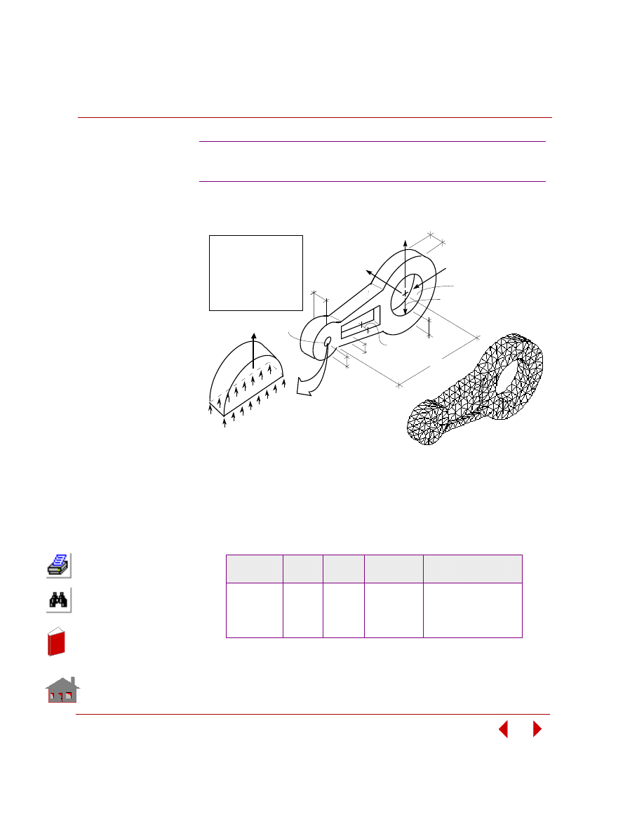
Chapter 5 Additional Problems
5-86
COSMOSM Advanced Modules
KEYWORDS:
Shape, static analysis, TETRA4, local sensitivity, stress response quantity.
PROBLEM:
Study the sensitivity of the steering control arm to changes in the thickness of the
shafts, size and location of the cutout. Perform a local sensitivity study by perturbing
the design variables by a ratio of 0.10. The arm outer thickness is 20 mm, modulus
of elasticity is 200,000 N/mm
2
and Poisson's ratio is 0.30
SUMMARY OF RESULTS:
SNSST1: Sensitivity Study of a Steering
Control Arm in Linear Stress Analysis
Design
Variables
Name
Initial
Value
Perturbation
Ratio
Gradient of Maximum
von Mises Stress
1
TR1
24
-0.10
-1.131
2
TR2
19
-0.10
1.1946
3
TW
8
-0.10
-11.324
4
DINT
6
+0.10
4.3820
tr
tw
= 31 N/mm
Y
TE TRA4 E LE ME NTS
X
Z
20
140
20
Internal surfaces
fixed in all directions
30
tr
1
7
I nit ia l P roble m
G e ome t ry
I nit ia l Finit e
E le me nt Me s h
dint
= 2 x 10 N/mm
= 0.3
E
Note: All dimensions
in milimeters.
ν
2
2
P
y
2
Y
P
y
5
In
de
x
In
de
x
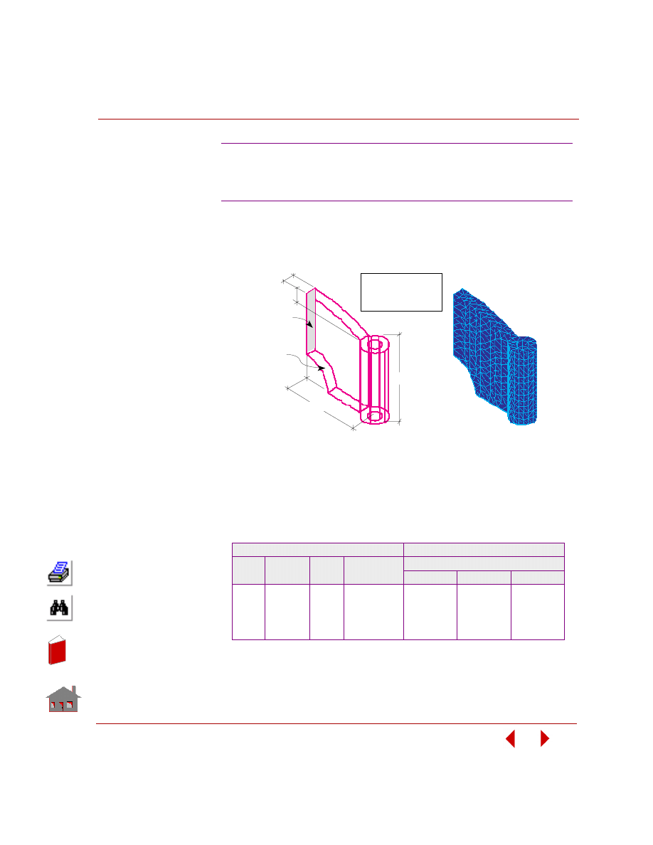
COSMOSM Advanced Modules
5-87
Part 2 OPSTAR / Optimization
KEYWORDS:
Shape, static analysis, TETRA10, primary and secondary load cases, local
sensitivity analysis, and stress response quantity.
PROBLEM:
Study the sensitivity of the bearing cap to changes in its dimensions. Perform a local
sensitivity study by perturbing the design variables by a ratio of 0.10. The bearing
cap modulus of elasticity is 200,000 N/mm
2
and Poisson's ratio is 0.30.
SUMMARY OF RESULTS
SNSST2: Sensitivity Study of an Engine
Bearing Cap in Stress Analysis Under
Multiple Load Cases
Design Variables
Gradient of Max von Mises Stress
Set
No.
Name
Initial
Value
Perturbation
Ratio
Load Case
1
2
51
1
ECCENT
75
-0.10
0.6238
1.4428
1.7547
2
TWEB
10
-0.10
1.7975
-12.318
-14.555
3
HEIGHT
70
-0.10
0.0633
-1.7607
-2.1395
4
HUMP
15
-0.10
0.03275
0.4751
1.6491
Fixed
ECCENT
Height
Initial
P roble m
Ge ome try
TWEB
Symmetry
Boundary
Conditions
HUMP
1 0 -Node Te tra Me sh
E
ν
= 2 x 10 N/mm
= 0.30
5
2
Initial Finite
E le me nt Me sh
In
de
x
In
de
x
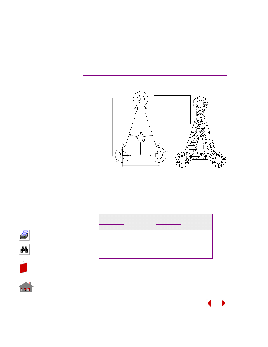
Chapter 5 Additional Problems
5-88
COSMOSM Advanced Modules
KEYWORDS:
Shape,
frequency
analysis,
SHELL3,
global
sensitivity,
frequency
response
quantity.
PROB-
LEM:
Study the
sensitivity
of the
fundamental
frequency of
the control arm bracket to changes in design variables. Use the global sensitivity
option by changing only one design variable at a time in 5 increments. The bracket
thickness is 0.3 cm, modulus of elasticity is 2 x 10
7
N/cm
2
Poisson's ratio is 0.3, and
mass density is 0.0075 Kg/cm
3
.
SUMMARY OR RESULTS:
SNSFQ1: Sensitivity Study of a Control
Arm Bracket in Frequency Analysis
Design
Variables
Fundamental
Frequency (Hz)
Design
Variables
Fundamental
Frequency (Hz)
T
1
T
2
T
1
T
2
0.5
3.5
8.6495
2.5
1.5
13.035
1.0
–
10.798
–
2.0
13.170
1.5
–
12.119
–
2.5
13.329
2.0
–
13.029
–
3.0
13.491
2.5
–
13.662
–
3.5
13.662
15.
0
1.5
1.0
Y
X
r = 1.0
r = 2.0
1.5
1.0
t
1
t
1
t
2
5.0
5.0
0.5
3 - Node Tria ngula r
Me s h ( S iz e = 1 )
= 0.3 cm
= 2 x 10 N/cm
= 0.30
= 0.0075 Kg/cm
7
2
Thickness
E
Note: All dimensions in centimeters.
3
ρ
ν
I nit ia l P roble m G e ome t ry
I nit ia l Finit e E le me nt Me s h
Fixed
Fixed
In
de
x
In
de
x
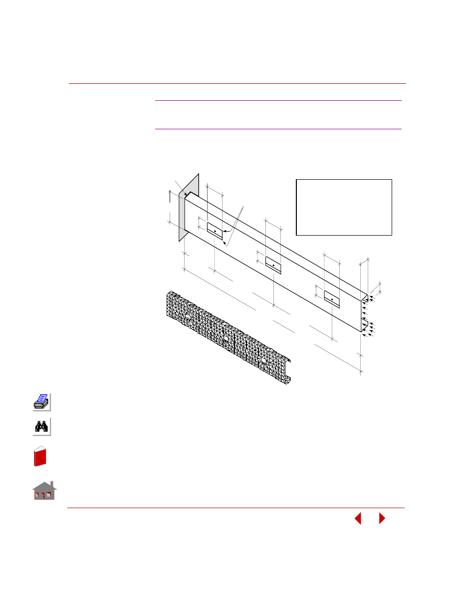
COSMOSM Advanced Modules
5-89
Part 2 OPSTAR / Optimization
KEYWORDS:
Shape, linearized buckling analysis, SHELL3, global sensitivity, buckling response
quantity.
PROBLEM:
Study the sensitivity of the column's buckling load factor to changes in design
variables. Change the design variables one at a time in 5 increments. The column
thickness is 0.25 inches, modulus of elasticity is 3 x 10
7
psi, Poisson's ratio is 0.28,
and material density is 0.73 x 10
-3
lb. sec
2
/in
4
.
SNSBK1: Sensitivity Study of a C-shape
Column in Linearized Buckling Analysis
I nit ia l Finit e
E le me nt Me s h
B = 20"
T
2
T
1
A = 6"
C = 3"
Fixed
T
2
T
1
T
2
T
1
h = 120"
0.18h
0.32h
0.32h
0.18h
p =
5,000 psi
(T /4)
2
Fillet
I nit ia l P roble m
G e ome t ry
= 3 in
= 0. 25 in
= A_ Steel
Element Size
Thickness
Material
S HE LL3
E
= 0.28
ν
= 3 x 10 psi
7
ρ
= 0.73 x 10 lbf sec /in
-3
2
4
In
de
x
In
de
x
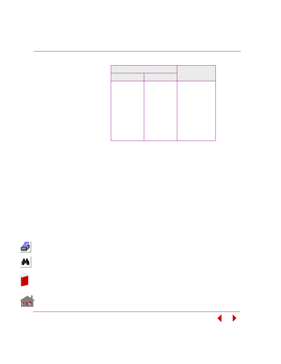
Chapter 5 Additional Problems
5-90
COSMOSM Advanced Modules
SUMMARY OR RESULTS:
Design Variables
Linearized Buckling
Load Factor
T
1
T
2
10.00
5
2.8069
16.25
—
2.7425
22.50
—
2.6475
28.75
—
2.5432
35.00
—
2.4502
10
5.00
2.8069
—
6.75
2.7630
—
8.50
2.6785
—
10.25
2.5992
—
12.00
2.5103
In
de
x
In
de
x
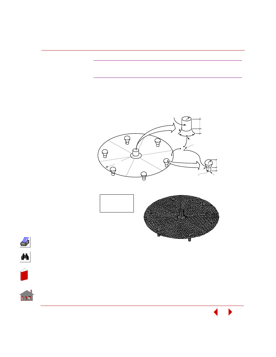
COSMOSM Advanced Modules
5-91
Part 2 OPSTAR / Optimization
KEYWORDS:
Shape and sizing, thermal analysis, SHELL3, global sensitivity, temperature
response quantity.
SNSHT1: Sensitivity Study of a Circular
Disk in Heat Transfer Analysis
Initial Finite E le me nt Me sh
25
10
5
= 2 mm
Thickness
3 - Node S he ll
Me s h ( S iz e = 2 )
10
5
5
5
2
Heat Flux
0.1 W/mm
Heat Flux
0.1 W/mm
2
Convection 0.0005 W/mm -
°
C
Ambient Temperature 50
°
C
2
Convection 0.0 W/mm -
°
C
Ambient Temperature 50
°
C
2
10
25
Radius
5
Initial P roble m Ge ome try
In
de
x
In
de
x
Chapter 5 Additional Problems
5-92
COSMOSM Advanced Modules
PROBLEM:
Study the sensitivity of the circular disk temperature to changes in thickness and
radius of the model. Use the global sensitivity feature and change one design
variable at a time. The disk conductivity is 0.57 W/mm-
°C. A convection of 0.0005
W/mm
2
-
°C with an ambient temperature of 50°C is applied to the entire model
except for the heat sources. The heat source regions (heat flux of 0.1 W/mm
2
) is
assumed to have a convection of 0 W/mm
2
-
°C with an ambient temperature of 50° C.
SUMMARY OR RESULTS:
Design Variables
Temperature
Radius
Thickness
30
2
144.6651
40
–
108.324
50
–
91.6635
60
–
82.8095
70
–
77.6308
70
0.500
111.055
–
0.875
92.2412
–
1.250
84.5067
–
1.625
80.2878
–
2.000
77.6308
In
de
x
In
de
x
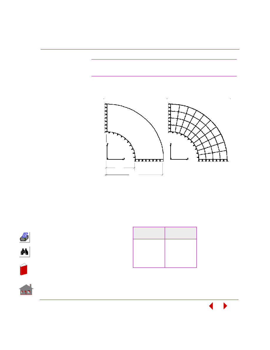
COSMOSM Advanced Modules
5-93
Part 2 OPSTAR / Optimization
KEYWORDS:
Shape, nonlinear analysis, von Mises plasticity, automatic time stepping,
PLANE2D, global sensitivity, and stress response quantity.
PROBLEM:
Study the sensitivity of the pipe to changes in the outer radius. The modulus of
elasticity is 86,666 psi, Poisson's ratio is 0.3, yield stress is 17.32 psi and tangential
modulus is 866 psi. Use the global sensitivity feature for 5 increments.
SUMMARY OF RESULTS:
SNSN1: Sensitivity Study of a Thick
Walled Pipe in Nonlinear Analysis
Design Variable:
ROUT
von Mises
Stress
1.50
25.0516
1.75
17.4911
2.0
17.3962
2.25
17.3580
2.50
17.3420
Rout
Initial P roble m Ge ome try
Rint
Initial Finite E le me nt Me sh
In
de
x
In
de
x
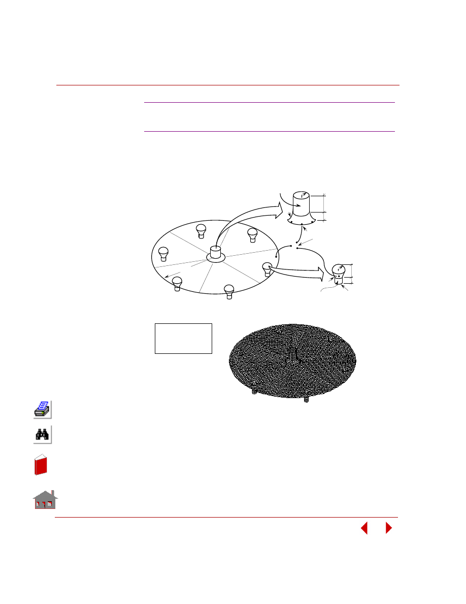
Chapter 5 Additional Problems
5-94
COSMOSM Advanced Modules
KEYWORDS:
Shape, thermal analysis, static analysis, frequency analysis, SHELL3,
TEMPREAD
,
local sensitivity, temperature, displacement and frequency response quantities.
SNSTSF1: Sensitivity Study of a Circular Disk in
Thermal, Stress and Frequency Analyses
Initial Finite E le me nt Me sh
25
10
5
= 2 mm
Thickness
3 - Node S he ll
Me s h ( S iz e = 2 )
10
5
5
5
2
Heat Flux
0.1 W/mm
Heat Flux
0.1 W/mm
2
Convection 0.0005 W/mm -
°
C
Ambient Temperature 50
°
C
2
Convection 0.0 W/mm -
°
C
Ambient Temperature 50
°
C
2
10
25
Radius
5
Initial P roble m Ge ome try
In
de
x
In
de
x
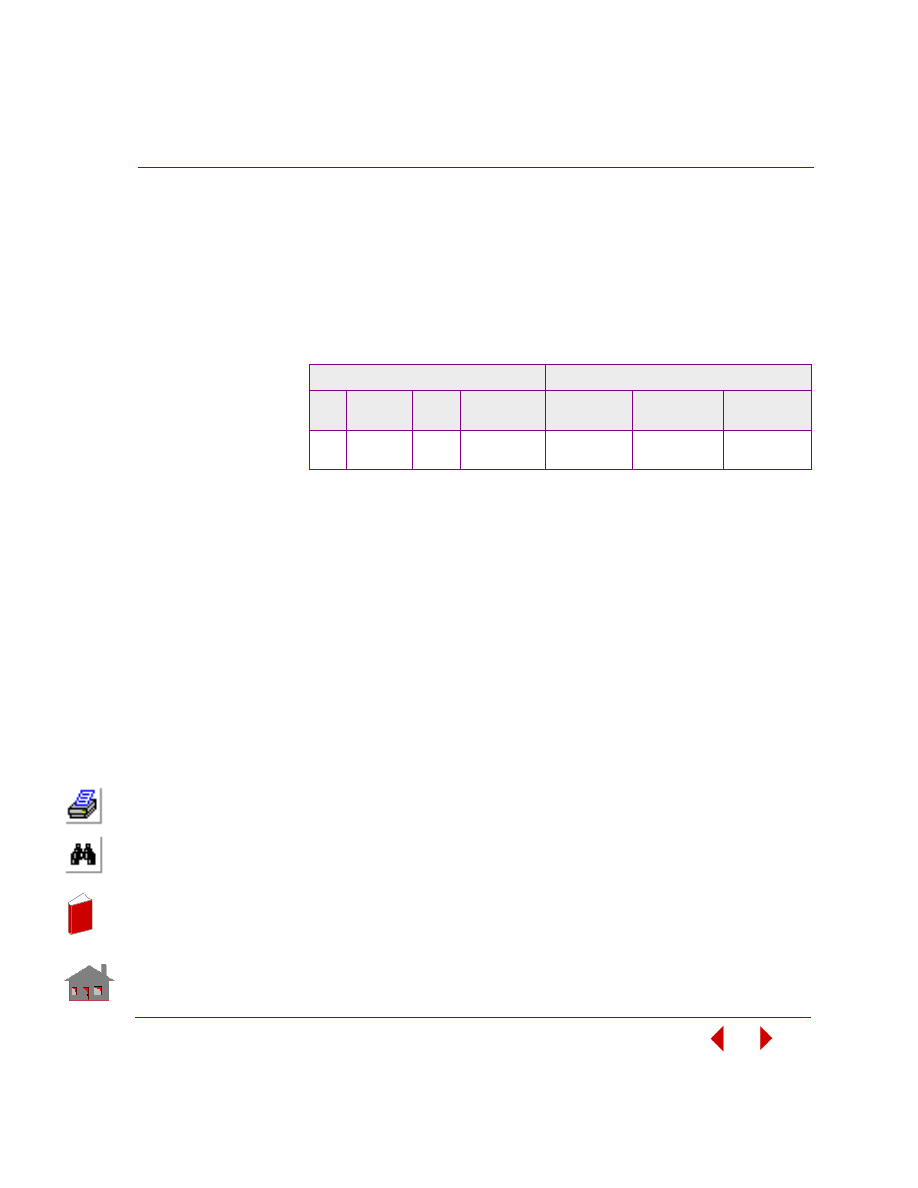
COSMOSM Advanced Modules
5-95
Part 2 OPSTAR / Optimization
PROBLEM:
Study the sensitivity of the circular disk response to changes is its thickness and
radius. Perform a local sensitivity study by perturbing the design variables by a ratio
of 0.1. The disk conductivity is 0.57 W/mm-
°C. A convection of 0.0005 W/mm
2
-
°C
with an ambient temperature of 50
°C is applied to the entire model except for the
heat sources. The heat source regions (heat flux of 0.1 W/mm-
°C) is assumed to have
a convection of 0 W/mm
2
-
°C with an ambient temperature of 50°C.
SUMMARY OF RESULTS
Design Variables
Gradient of Response Quantities
Set
No.
Name
Initial
Value
Perturbation
Ratio
Temperature
Resultant
Displacement
Fundamental
Frequency
1
Radius
70
-0.10
-0.4415
+0.003120
-0.04806
2
Thickness
1.8
-0.10
-6.3049
-0.01540
+0.5076
In
de
x
In
de
x
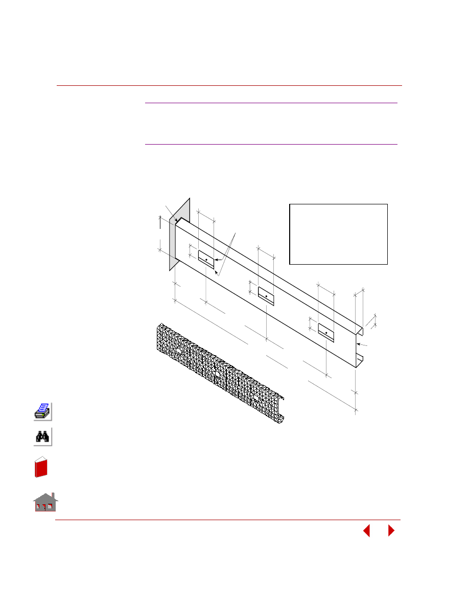
Chapter 5 Additional Problems
5-96
COSMOSM Advanced Modules
KEYWORDS:
Shape, thermal analysis, static analysis, buckling analysis, SHELL3,
TEMPREAD
,
global sensitivity, buckling load factor, displacement and temperature response
quantities.
SNSTSB1: Sensitivity Study of a
C-shape Column in Thermal,
Stress and Buckling Analyses
I nit ia l Finit e
E le me nt Me s h
B = 20"
T
2
T
1
A = 6"
C = 3"
Fixed
T
2
T
1
T
2
T
1
h = 120"
0.18h
0.32h
0.32h
0.18h
(T /4)
2
Fillet
I nit ia l P roble m
G e ome t ry
= 3 in
= 0. 25 in
= A_ Steel
Element Size
Thickness
Material
S HE LL3
E
= 0.28
ν
= 3 x 10 psi
7
ρ
= 0.73 x 10 lbf sec /in
-3
2
4
Fixed
In
de
x
In
de
x
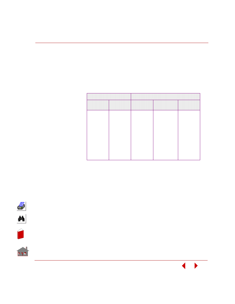
COSMOSM Advanced Modules
5-97
Part 2 OPSTAR / Optimization
PROBLEM:
Study the sensitivity of the C-Shape column to changes in the cutouts sizes. Change
design variables one at a time in 5 increments. The cross section thickness is 0.25
inch, modulus of elasticity is 3 x 10
7
psi, and Poisson's ratio is 0.28. The material
conductivity is 6.7E-4 BTU/in/s
°F. A convection of 0.0001 BTU/sec in
2
-
°F with an
ambient temperature of 50
°F and a volume heat of 0.005 BTU/sec in
3
are applied for
the entire model. The material's coefficient of thermal expansion is 7.4E-6/
°F.
SUMMARY OR RESULTS:
Design Variables
Response Quantities
T1
T2
Max Temp
Max Resultant
Displ.
Buckling
Load Factor
10.00
5
88.316
0.01299
1.8271
16.25
5
89.275
0.01739
1.7903
22.50
5
90.325
0.02204
1.7771
28.75
5
90.713
0.02327
1.8015
35.00
5
90.939
0.01941
1.8406
10.00
5.00
88.316
0.01299
1.8271
10.00
6.75
89.402
0.01294
2.1557
10.00
8.50
89.321
0.01232
2.5762
10.00
10.25
88.905
0.01235
2.9213
10.00
12.00
89.674
0.01306
3.1636
In
de
x
In
de
x
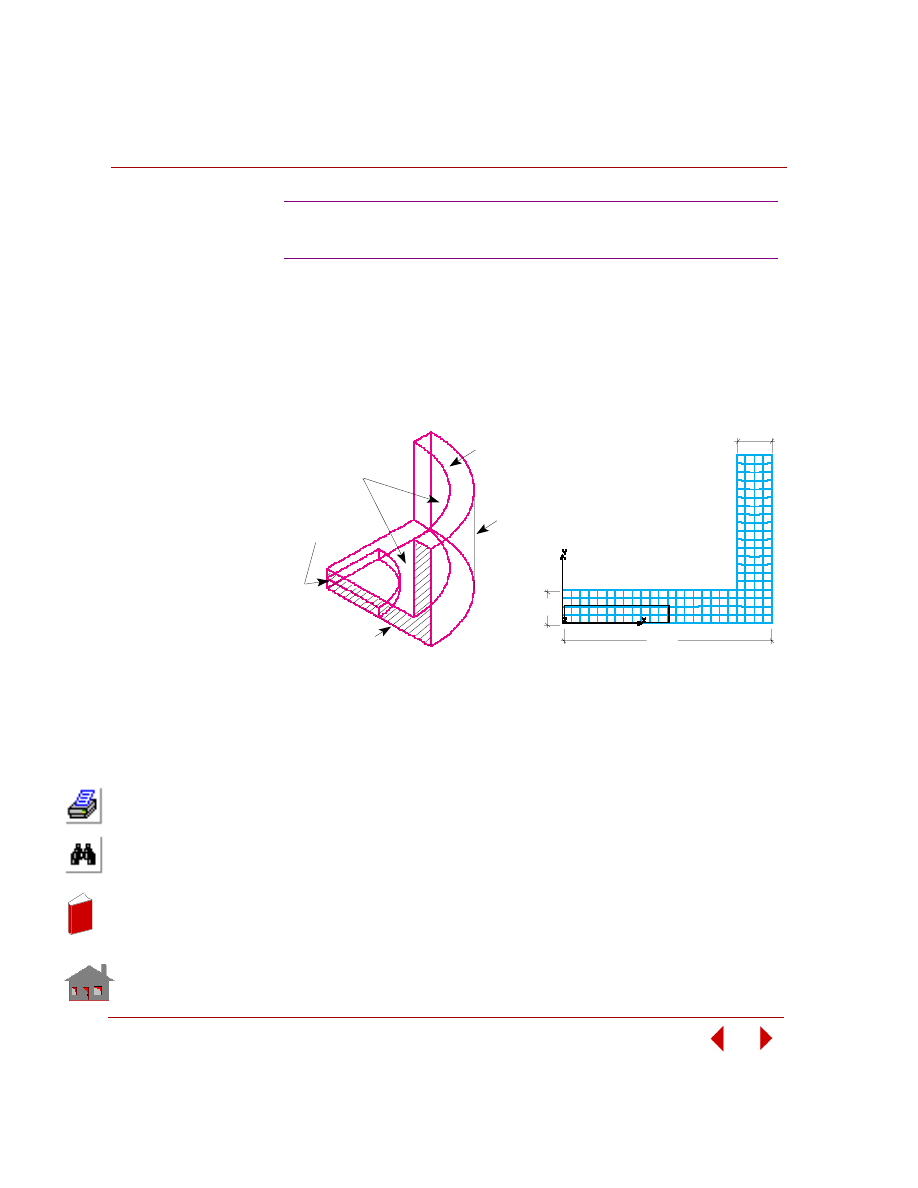
Chapter 5 Additional Problems
5-98
COSMOSM Advanced Modules
KEYWORDS:
Shape, transient thermal, nonlinear analysis, radiation, convection, heat flux,
element heat, prescribed temperatures, multi-disciplinary global sensitivity study,
von Mises plasticity, Axisymmetric PLANE2D, stress, strain and temperature
response quantities.
PROBLEM:
Study the sensitivity of a cylinder to changes in its outer diameters and thickness.
Change the design variables one at a time in 5 increments. Steel alloy and aluminum
materials are used.
SNSTN1: Sensitivity Study of a Cylinder in
Intransient Thermal and Nonlinear Analyses
Thick
Initia l Finite Ele me nt Me sh
Initia l Ge ome try, Loa ds
a nd Bounda ry C onditions
Thic
k
ROUT
Temperature = 70
°
F
Radiation Source
Emissivity
View Factor
= 500
°
F
= 0.9
= 0.8
Ambient
Temperature = 200
°
F
Firm Coefficient
= 0.1 BTU /
(sec in in
°
F)
_
Convection
Element
Heat
= 0.140625 BTU /
(sec in in in)
Heat Flux
= 0.0125 BTU /
(sec in in)
In
de
x
In
de
x
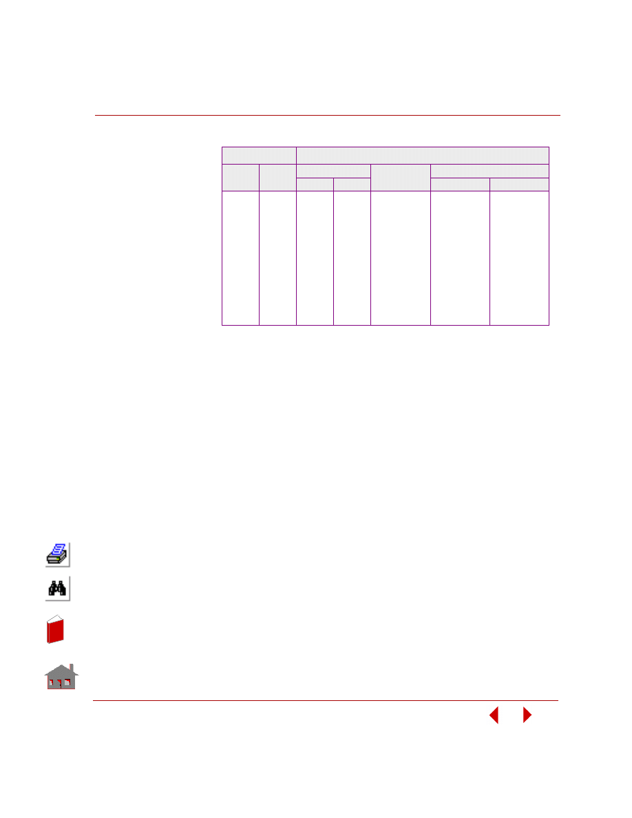
COSMOSM Advanced Modules
5-99
Part 2 OPSTAR / Optimization
SUMMARY OF RESULTS:
Design Variables
Response Quantities
ROUT
Thick
von Mises
Temperature
Eff. Strain
1
2
1
2
5.00
2.000
57,563
31,415
570.292
0.5043E-2
0.4254E-2
6.75
–
57,911
30,495
509.935
0.5094E-2
0.3051E-2
8.50
–
52,877
30,283
470.377
0.4670E-2
0.2569E-2
10.25
–
47,987
30,315
439.297
0.4247E-2
0.2536E-2
12.00
–
44,040
30,217
413.634
0.3896E-2
0.2109E-2
12.00
0.500
22,894
22,724
260.386
0.2025E-2
0.0839E-2
–
0.875
28,577
27,551
304.249
0.2525E-2
0.1085E-2
–
1.250
34,039
29,361
345.801
0.3012E-2
0.1371E-2
–
1.625
39,259
30,130
382.817
0.3472E-2
0.1782E-2
–
2.000
44,040
30,217
413.634
0.3896E-2
0.2109E-2
In
de
x
In
de
x
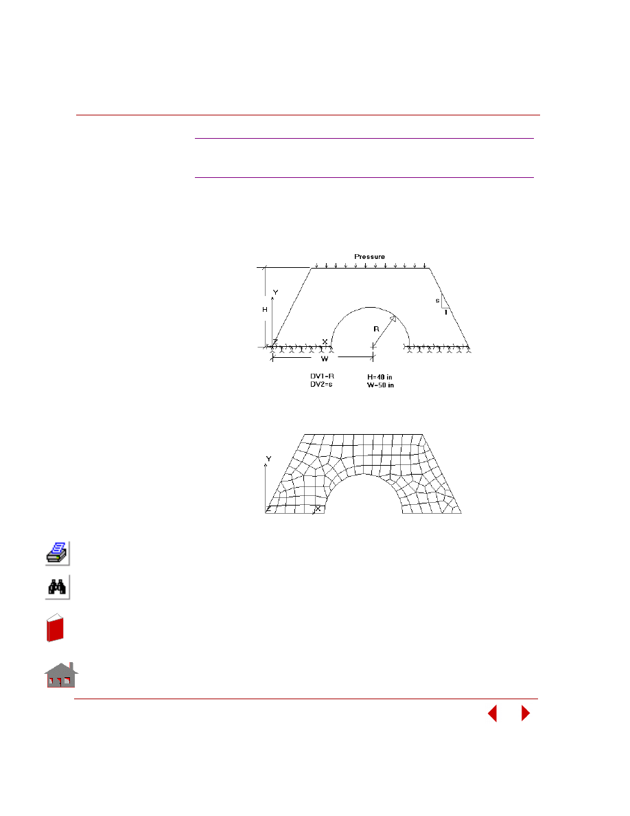
Chapter 5 Additional Problems
5-100
COSMOSM Advanced Modules
KEYWORDS:
Frequency analysis, post-dynamic analysis (harmonic response), dynamic stress
analysis, 4-noded PLANE2D elements, shape, offset sensitivity, frequency,
displacement, and stress response quantities.
Initial Problem Geometry
Initial Finite Element Mesh
SNSFDS1: Sensitivity Study of a Culvert
in Harmonic Response Analysis
In
de
x
In
de
x
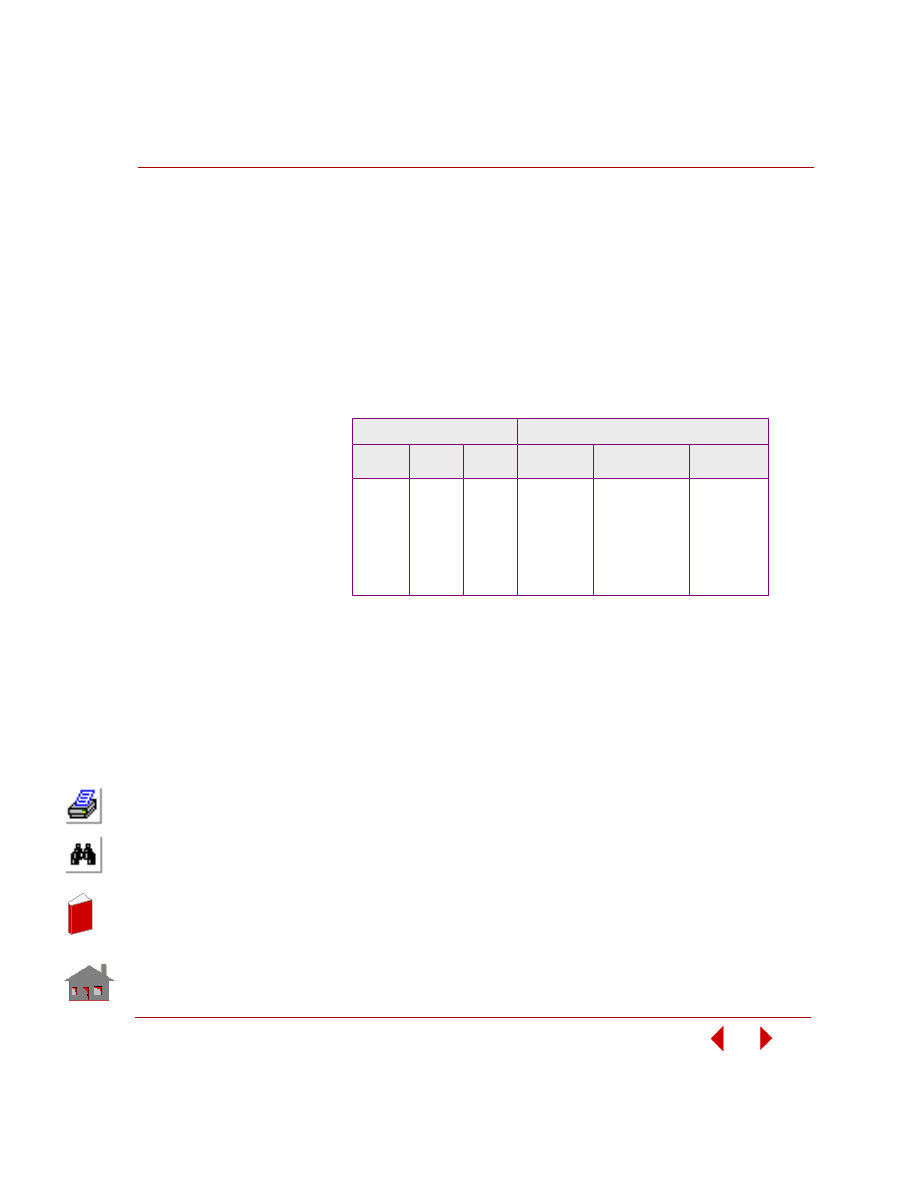
COSMOSM Advanced Modules
5-101
Part 2 OPSTAR / Optimization
PROBLEM:
Study the sensitivity of a culvert due to changes in the design variables, radius R and
slope s. The material constants of the culvert are given as: Young’s modulus E =
30E6 psi, Poisson’s ratio
υ = 0.3, and Density ρ = 1. lb*sec
2
/in
4
. A harmonic
pressure loading with constant amplitude 500 psi within the desired range of
frequency (1 rad/sec - 400 rad/sec) is applied to the top of the culvert. A modal
damping 0.015 is assumed for the first 10 modes. Six sets of design variables and
their respective results are listed in the following table. Note that the response
quantities, displacement and stress, are defined as the extreme values within the
desired range of frequency.
SUMMARY OF RESULTS:
Design Variables
Response Quantities
Set
Number
DV1
(R)
DV2
(s)
Frequency
(1st)
Displacement
(Uy)
Stress
(von Mises)
1
20
2.0
16.181
0.0429
4.7188E4
2
23
1.86
14.851
0.0575
5.3807E4
3
26
1.7
13.354
0.0803
6.2323E4
4
29
1.55
11.684
0.1177
8.0398E4
5
32
1.4
9.5110
0.1948
1.2790E5
6
35
1.3333
6.8929
0.4574
2.3871E5
In
de
x
In
de
x
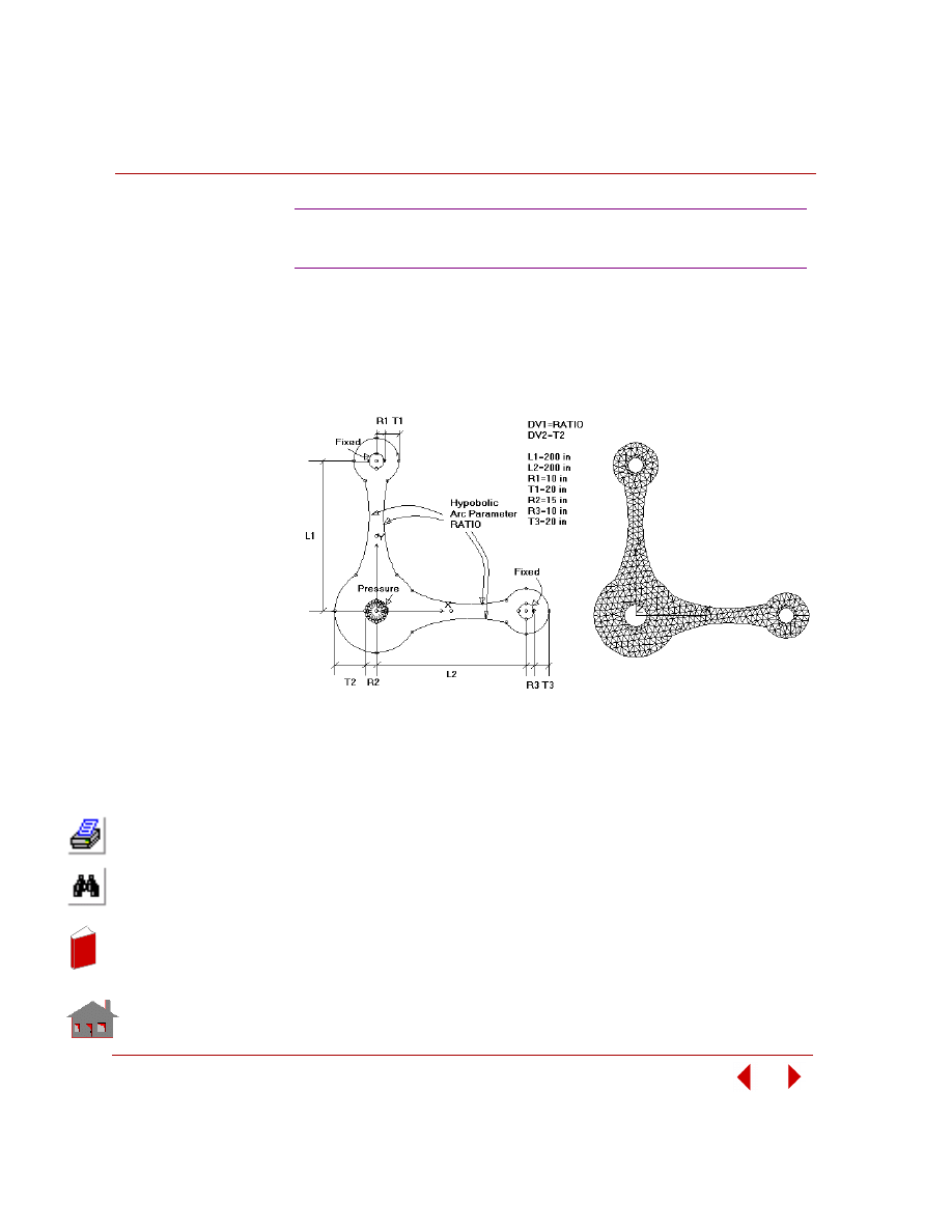
Chapter 5 Additional Problems
5-102
COSMOSM Advanced Modules
KEYWORDS:
Frequency analysis, post-dynamic analysis (random vibration), dynamic stress
analysis, 6-noded TRIANG elements, shape, global sensitivity (one-by-one),
frequency, displacement, and stress response quantities.
SNSFDS2: Sensitivity Study of a Lever
Arm in Random Vibration Analysis
Initial Problem Geometry
Initial Finite
Element Mesh
In
de
x
In
de
x
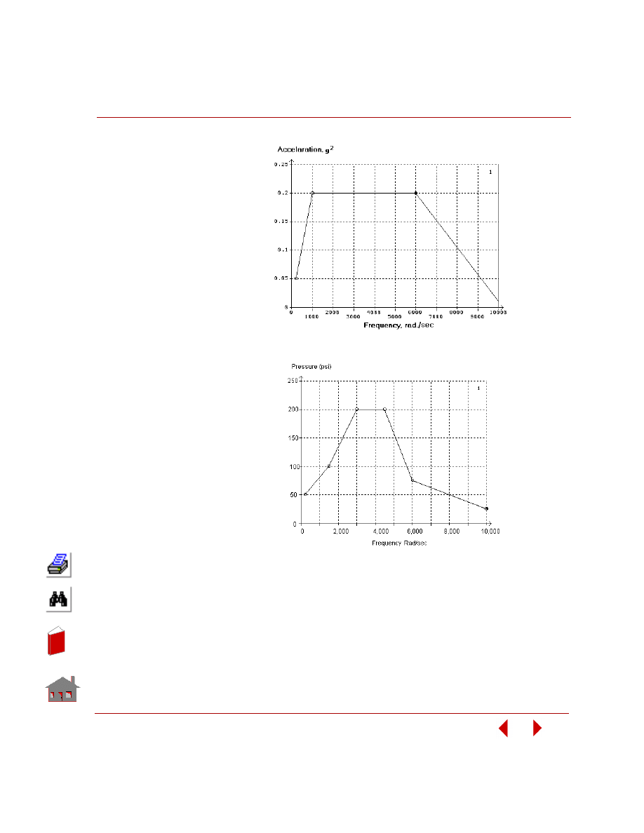
COSMOSM Advanced Modules
5-103
Part 2 OPSTAR / Optimization
Base Excitation versus Frequency Curve
Pressure Loading versus Frequency Curve
PROBLEM:
Study the sensitivity of a lever arm due to changes in the design variables, hyperbolic
arc parameter RATIO and thickness T2. The arm is made of A_STEEL and has a
uniform thickness 1.0 in. Both harmonic pressure loading and base excitation
(acceleration) in the y-direction are applied to the structure as shown in the figure.
A modal damping 3% is assumed for the first 5 modes. Changing one design variable
In
de
x
In
de
x
Chapter 5 Additional Problems
5-104
COSMOSM Advanced Modules
at a time in 5 increments, their values and the respective results are listed in the
following table. Note that the response quantity, displacement, is defined as the
extreme value of PSD within the desired range of frequency and the stress is the
extreme value of RMS.
SUMMARY OF RESULTS:
Design Variables
Response Quantities
DV1
(RATIO)
DV2
(T2)
Frequency
(1st)
Displacement
(U
y
)
Stress
(von Mises)
0.5
40.0
92.563
3.1740E-4
1.1834E4
0.5625
-
87.351
3.2949E-4
1.2498E4
0.625
-
81.806
3.4710E-4
1.3734E4
0.6875
-
75.813
3.7408E-4
1.5190E4
0.75
-
69.242
4.1664E-4
1.7617E4
0.5
15.0
85.956
2.3235E-4
7710.6
-
23.75
89.917
1.6545E-4
9111.7
-
32.5
92.059
2.1621E-4
1.1198E4
-
41.25
92.524
3.1188E-4
1.1832E4
-
50.0
91.206
2.2683E-4
1.1321E4
In
de
x
In
de
x
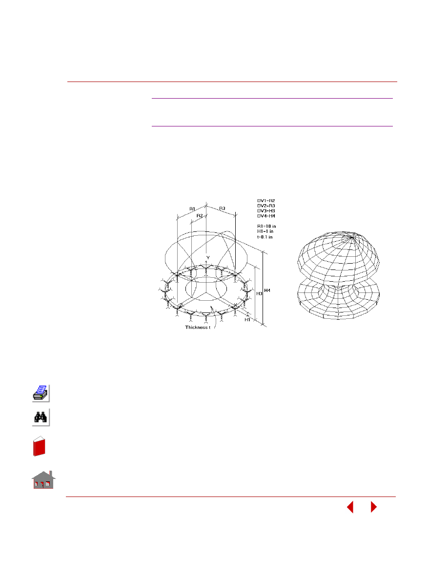
COSMOSM Advanced Modules
5-105
Part 2 OPSTAR / Optimization
KEYWORDS:
Frequency analysis, post-dynamic analysis (response spectrum analysis), dynamic
stress analysis, SHELL4 elements, shape, local sensitivity, frequency, displacement,
and stress response quantities.
SNSFDS3: Sensitivity Study of a Trophy
in Response Spectrum Analysis
Initial Problem Geometry
Initial Finite
Element Mesh
In
de
x
In
de
x
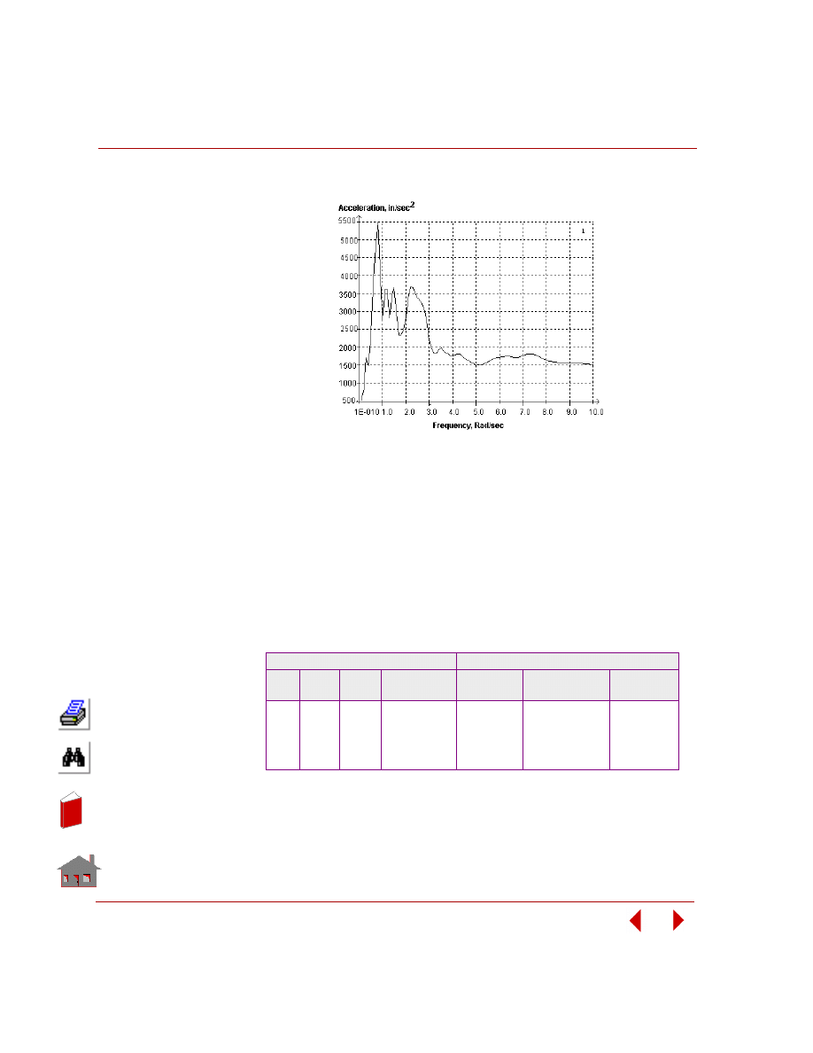
Chapter 5 Additional Problems
5-106
COSMOSM Advanced Modules
Acceleration Spectrum Excitation
PROBLEM:
Study the sensitivity of a trophy due to changes in its dimensions, R2, R3, H3, and
H4. The trophy is made of A_STEEL and has a 5% critical damping. The base of the
trophy is experiencing an acceleration spectrum excitation as shown in the figure.
Performing a local sensitivity study by perturbing all the design variables by a ratio
+0.05, the gradients of the response quantities are listed in the following table. Note
that the response quantities, displacement and stress, are defined as the extreme
values by using the SRSS mode combination method.
SUMMARY OF RESULTS:
Design Variables
Gradients of Response Quantities
Set
No.
Name
Initial
Value
Perturbation
Ratio
Frequency
(1st)
Displacement
(U
x
)
Stress
(von Mises)
1
R2
5
+0.05
9.8388
-0.0393
-1241.5
2
R3
10
+0.05
-2.4151
9.0626E-3
475.12
3
H3
10
+0.05
-0.4585
4.3791E-4
116.50
4
H4
21
+0.05
-1.1676
8.1406E-3
219.92
In
de
x
In
de
x

COSMOSM Advanced Modules
5-107
Sizing Sensitivity Problems
In
de
x
In
de
x
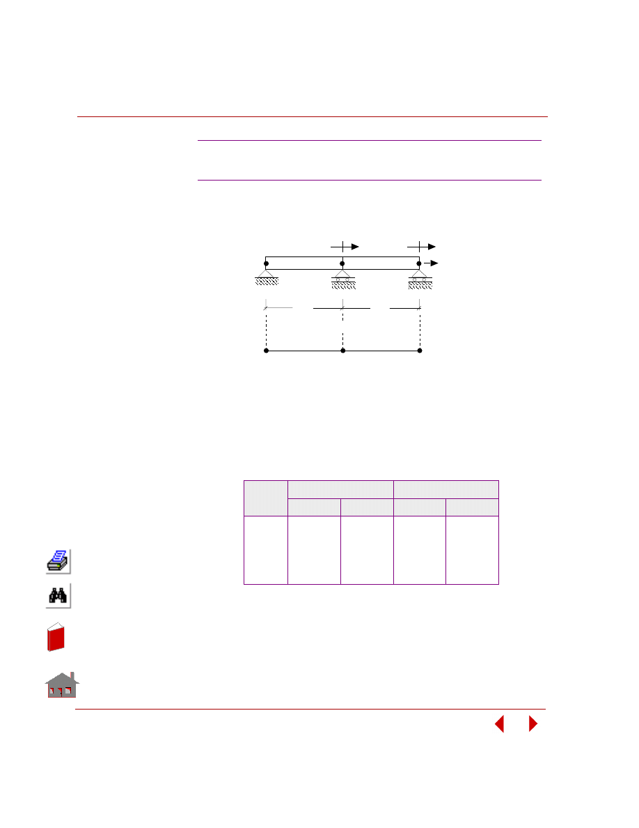
Chapter 5 Additional Problems
5-108
COSMOSM Advanced Modules
KEYWORDS:
Sizing, static analysis, TRUSS2D, global sensitivity.
PROBLEM:
Study the behavior of the 2-bar truss for different values of cross sectional areas A
1
,
and A
2
. The length of each bar is 30 inches and modulus of elasticity is 5 psi. The
design variables are to be changed simultaneously in 5 increments.
SUMMARY OF RESULTS:
SNZST1: Global Sensitivity of a 2-bar Truss: All
Design Variables Incremented Simultaneously
Run
Number
Design Variables
Response Quantities
A
1
A
2
U
2
U
3
1
1.000
1.000
60.000
120.000
2
3.250
3.250
18.462
36.923
3
5.500
5.500
10.909
21.818
4
7.750
7.750
7.7419
15.484
5
10.000
10.000
6.000
12.000
F = 10 lbs
P roble m Ge ome try
Finite E le me nt Me sh
30"
A
A
30"
1
2
1
2
3
U
2
U
3
In
de
x
In
de
x
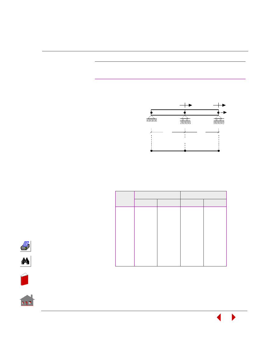
COSMOSM Advanced Modules
5-109
Part 2 OPSTAR / Optimization
KEYWORDS:
Sizing, static analysis,
TRUSS2D, global
sensitivity.
PROBLEM:
Study the behavior of the
2-bar truss for different
values of cross sectional
areas A
1
, and A
2
. The
length of each bar is 30
inches and modulus of
elasticity is 5 psi. The
design variables are to be
changed one at a time in
5 increments.
SUMMARY OF RESULTS:
SNZST2: Global Sensitivity of a 2-bar Truss:
Design Variables Incremented One at a Time
Run
Number
Design Variables
Response Quantities
A
1
A
2
U
2
U
3
1
1.0
1.0
60.000
120.000
2
3.25
1.0
18.462
78.462
3
5.50
1.0
10.909
70.909
4
7.75
1.0
7.7419
67.742
5
10.00
1.0
6.000
66.000
6
1.0
1.0
60.000
120.000
7
1.0
3.25
60.000
78.462
8
1.0
5.50
60.000
70.909
9
1.0
7.75
60.000
67.742
10
1.0
10.00
60.000
66.000
F = 10 lbs
P roble m Ge ome try
Finite E le me nt Me sh
30"
A
A
30"
1
2
1
2
3
U
2
U
3
In
de
x
In
de
x
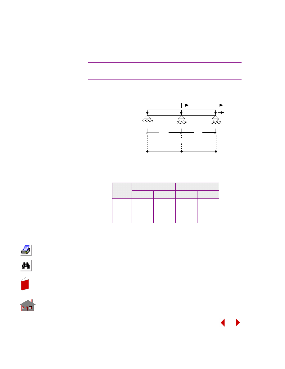
Chapter 5 Additional Problems
5-110
COSMOSM Advanced Modules
KEYWORDS:
Sizing, static, TRUSS2D,
offset sensitivity.
PROBLEM:
Study the behavior of the
2-bar truss for specified
values of cross sectional
areas A
1
, and A
2
. The
length of each bar is 30 in
and modulus of elasticity
is 5 psi. Four different sets
are used to specify design
variables.
SUMMARY OF RESULTS:
SNZST3: Offset Sensitivity of a 2-bar Truss
Set
Number
Design Variables
Response Quantities
A
1
A
2
U
2
U
3
1
1.0
10.0
60.0
66.0
2
10.0
1.0
6.0
66.0
3
10.0
10.0
6.0
12.0
4
5.0
5.0
12.0
24.0
F = 10 lbs
P roble m Ge ome try
Finite E le me nt Me sh
30"
A
A
30"
1
2
1
2
3
U
2
U
3
In
de
x
In
de
x
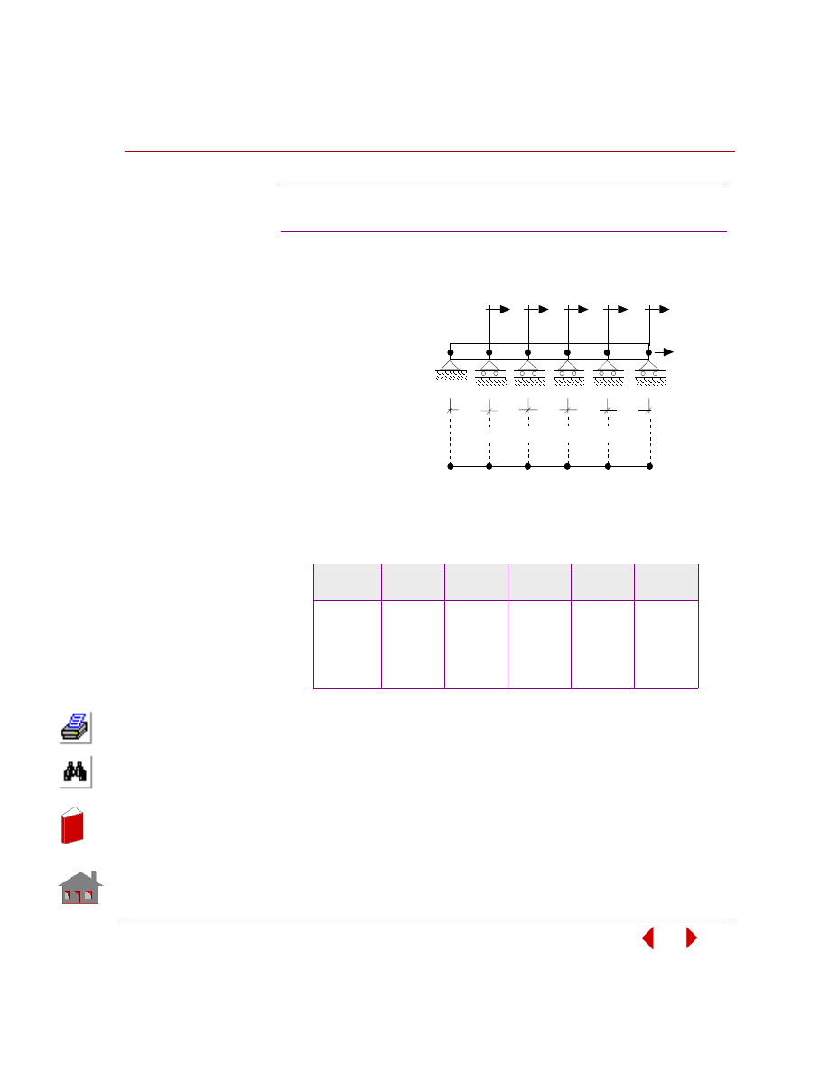
COSMOSM Advanced Modules
5-111
Part 2 OPSTAR / Optimization
KEYWORDS:
Sizing, static,
TRUSS2D, local
sensitivity.
PROBLEM:
Study the effect of
changing (perturbing)
design variables on the
response of a 5-bar truss.
The cross-sectional area
of each bar is 1.0 in,
length is 10 in (each) and
modulus of elasticity is 5
psi. Each design variable
is perturbed by 10%.
SUMMARY OF RESULTS:
SNZST4: Local Sensitivity of a 5-bar Truss
Design
Variable
U
1
*
U
2
*
U
3
*
U
4
*
U
5
*
A1
-18.1818
-18.1818
-18.1818
-18.1818
-18.1818
A2
0.0
-18.1818
-18.1818
-18.1818
-18.1818
A3
0.0
0.0
-18.1818
-18.1818
-18.1818
A4
0.0
0.0
0.0
-18.1818
-18.1818
A5
0.0
0.0
0.0
0.0
-18.1818
*Derivative of Response Quantity with Respect to Design Variables
3
10"
10"
10"
10"
10"
F = 10 lbs
P roble m Ge ome try
Finite E le me nt Me sh
A
1
1
6
U
2
A
2
A
3
A
A
5
4
2
U
3
U
4
U
5
U
6
4
5
In
de
x
In
de
x
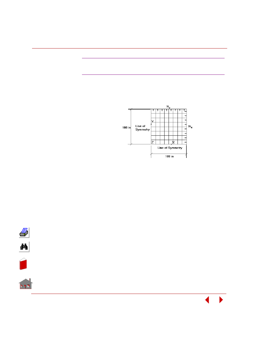
Chapter 5 Additional Problems
5-112
COSMOSM Advanced Modules
KEYWORDS:
Linear static analysis, SHELL4L elements, size (ply orientation), global sensitivity,
maximum failure index response quantity.
PROBLEM:
Study the sensitivity of a 6-layer [-
θ / 0 / θ]
s
Graphite-Epoxy laminate due to changes
in the ply orientation
θ. The total thickness of 6 plies is 1 inch. The material
constants are given as: modulus of elasticity in the first material direction E
x
=
26.27E6 psi, modulus of elasticity in the second material direction E
y
= 1.49E6 psi,
Poisson’s ratio
υ = 0.28, shear modulus in the material first-second plane G
xy
=
1.04E6 psi, tensile and compressive strengths in the 1st material direction F
1T
= F
1C
= 2.17E5 psi, tensile and compressive strengths in the second material direction F
2T
= 5.81E3 psi and F
2C
= 3.57E4 psi, shear strength in the material first-second plane
F
12
= 9.87E3 psi. A biaxial tensile loading is applied to the edges of the structure
with the ratios of the transverse load (N
y
) to the longitudinal load (N
x
) equal to 0,
0.5, and 1.0 where N
x
= 100 psi. Changing the ply orientation in 10 increments, their
values and the respective maximum failure indexes are listed in the following table.
SNZST5: Sensitivity Study of a
Graphite-epoxy Laminate
Initial Problem Geometry and Finite Element Mesh
In
de
x
In
de
x
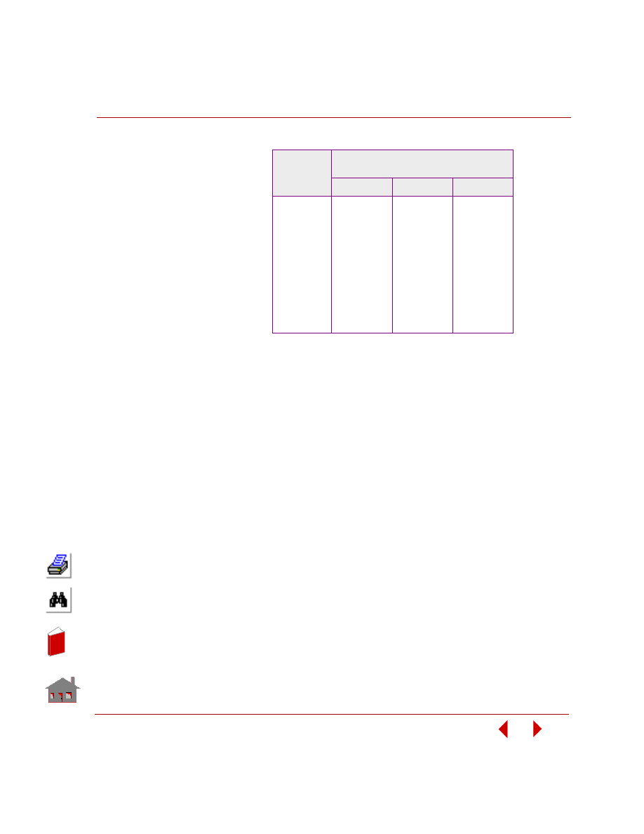
COSMOSM Advanced Modules
5-113
Part 2 OPSTAR / Optimization
SUMMARY OF RESULTS:
Design
Variable,
q
Response Quantity,
Maximum Failure Index
N
y
/N
x
= 0
N
y
/N
x
= 0.5
N
y
/N
x
= 1
1E-16 (=0)
2.1236E-7
7.2160E-3
0.01446
10
-2.3987E-4
6.7899E-3
0.01384
20
-8.2275E-4
5.4160E-3
0.01167
30
-1.2468E-3
3.3621E-3
7.9831E-3
40
-1.0689E-3
1.7210E-3
4.5160E-3
50
7.8222E-4
1.3938E-3
2.6199E-3
60
1.4606E-3
1.6914E-3
1.9231E-3
70
1.8906E-3
2.0304E-3
2.1705E-3
80
2.1198E-3
2.2559E-3
2.3923E-3
90
2.1912E-3
2.3327E-3
2.4743E-3
In
de
x
In
de
x
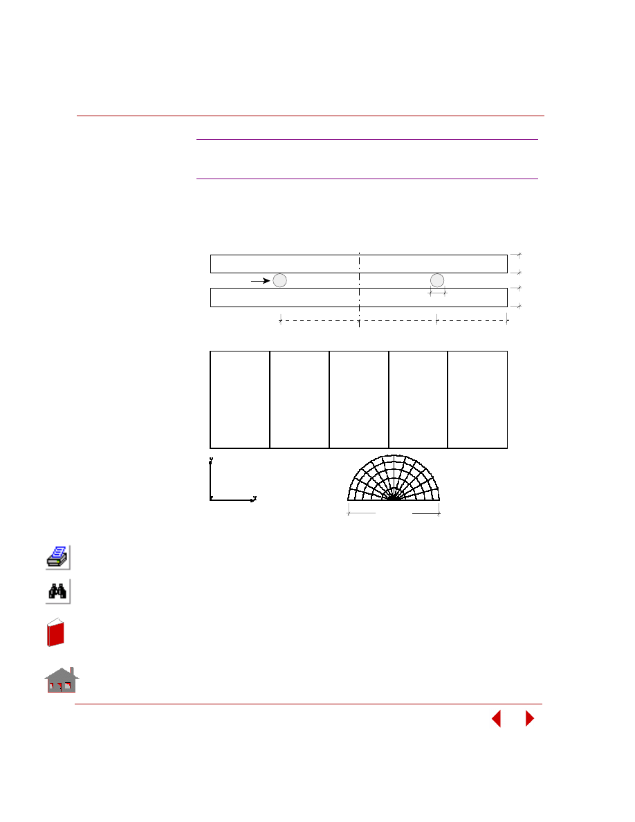
Chapter 5 Additional Problems
5-114
COSMOSM Advanced Modules
KEYWORDS:
Shape, nonlinear analysis, rubber, Mooney model, contact, prescribed displacement,
automatic time stepping, axisymmetric PLANE2D, friction, and stress response
quantity.
SNZN1: Sensitivity of a Rubber Circular Ring to
Coefficient of Friction in Nonlinear Analysis
0.5615"
Initial Finite E le me nt Me sh
0.5615"
0.3475"
Top Steel Plate
Bottom Steel Plate
Initial P roble m Ge ome try
2 R Cross
0.3"
0.3"
0.278"
Rubber Ring
In
de
x
In
de
x
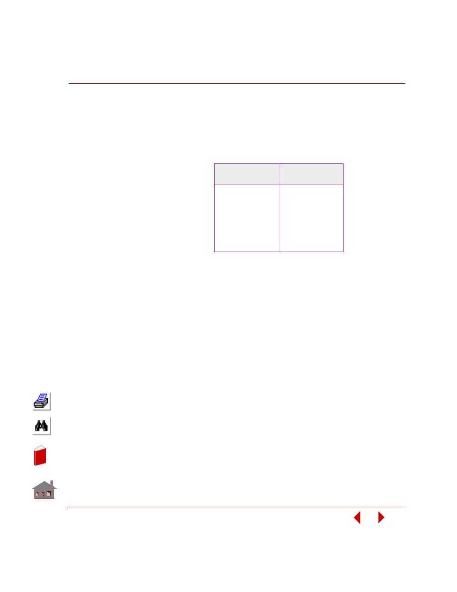
COSMOSM Advanced Modules
5-115
Part 2 OPSTAR / Optimization
PROBLEM:
Study the sensitivity of circular ring response to the friction coefficient value. Use
the global sensitivity option. For rubber, the Mooney's constants are 175 and 10 psi,
and the Poisson's ratio is 0.49. For steel plates, the Young's modulus is 30 x 10
6
psi,
and Poisson's ratio is 0.3.
SUMMARY OF RESULTS:
Design Variable:
FRICTION
von Mises Stress
in Rubber Ring
0.01
209.218
0.05
217.170
0.09
226.550
0.13
233.667
0.17
232.391
0.21
229.952
0.25
230.037
In
de
x
In
de
x

5-116
COSMOSM Advanced Modules
In
de
x
In
de
x
COSMOSM Advanced Modules
I-1
Index
A
analysis
approximations
automatic time stepping
B
beam height
beam width
behavior constraints
bending
buckling
buckling response quantity
C
contact
convection
converged
convergence
curves
D
design optimization
design variables
displacement constraint
33, 5-37, 5-39, 5-42, 5-45, 5-48, 5-
53, 5-57, 5-60, 5-63, 5-65
displacement response
quantity
E
effective strain constraint
element heat
F
failure index response quantity
frequency analysis
frequency constraint
31, 5-37, 5-39, 5-42, 5-48, 5-73, 5-
frequency response quantity
friction
G
global sensitivity
5-91, 5-93, 5-96, 5-98, 5-102, 5-108,
5-109, 5-112
H
heat transfer
L
limit point
limits
linearized buckling
local sensitivity
M
mass constraint
modified feasible directions
Mooney model
multidisciplinary design
optimization
multidisciplinary optimization
26, 5-28, 5-31, 5-33, 5-37, 5-39, 5-
multiple load cases
N
natural frequency
nonlinear
numerical techniques
In
de
x
In
de
x
Index
I-2
COSMOSM Advanced Modules
O
objective function
optimization loops
P
PLANE2D
prescribed displacement
R
restart
restore
S
sensitivity
shape optimization
shape sensitivity
singular value decomposition
sizing
static
stress constraint
stress response quantity
5-93, 5-100, 5-102, 5-105, 5-114
T
temperature response quantity
trimming factors
truncation
types of sensitivity
W
weight factors
In
de
x
In
de
x
Document Outline
- COSMOSM Optimization Module (OPTSTAR)
- 1 Introduction
- 2 Elements of Optimization and Sensitivity
- 3 Procedures and Examples
- 4 Numerical Aspects
- 5 Additional Problems
- Index
Wyszukiwarka
Podobne podstrony:
Herbs for Sports Performance, Energy and Recovery Guide to Optimal Sports Nutrition
Comarch CDN OPTIMA Pulpit Menadzera 4 1 wersja online
Module 10
Module 8
Food ćwiczenia angielski Starland 1 module 8
Instrukcja montażu sufitów podwieszanych w module 600x600mm System standardowy 600x600 1 AMF REINRAU
AT Commands for Bluetooth Module
Module 07
CISCO CCNA Certifications CCNA 2 Module 10
CISCO CCNA Certifications CCNA 2 Module 9
Module 12
CISCO CCNA Certifications CCNA 2 Module 1
delta module1 sample test01 1
06 BS Module 1 Section 6
CISCO CCNA Certifications CCNA 3 Module 3
IBD optimal
Module 11
CISCO CCNA Certifications CCNA 2 Module 8
więcej podobnych podstron