Stinchcombe M B , Notes for a Course in Game Theory

Notes for a Course in Game Theory

Maxwell B. Stinchcombe

Fall Semester, 2002. Unique #29775

Chapter 0.0

Contents

Organizational Stuff

Choice Under Uncertainty

1.1

The basics model of choice under uncertainty . . . . . . . . . . . . . . . . . .

1.1.1

Notation . . . . . . . . . . . . . . . . . . . . . . . . . . . . . . . . . .

1.1.2

The basic model of choice under uncertainty . . . . . . . . . . . . . .

1.1.3

Examples . . . . . . . . . . . . . . . . . . . . . . . . . . . . . . . . .

1.2

The bridge crossing and rescaling Lemmas . . . . . . . . . . . . . . . . . . .

1.3

Behavior . . . . . . . . . . . . . . . . . . . . . . . . . . . . . . . . . . . . . .

1.4

Problems . . . . . . . . . . . . . . . . . . . . . . . . . . . . . . . . . . . . . .

Correlated Equilibria in Static Games

2.1

Generalities about static games . . . . . . . . . . . . . . . . . . . . . . . . .

2.2

Dominant Strategies . . . . . . . . . . . . . . . . . . . . . . . . . . . . . . .

2.3

Two classic games . . . . . . . . . . . . . . . . . . . . . . . . . . . . . . . . .

2.4

Signals and Rationalizability . . . . . . . . . . . . . . . . . . . . . . . . . . .

2.5

Two classic coordination games . . . . . . . . . . . . . . . . . . . . . . . . .

2.6

Signals and Correlated Equilibria . . . . . . . . . . . . . . . . . . . . . . . .

2.6.1

The common prior assumption . . . . . . . . . . . . . . . . . . . . . .

2.6.2

The optimization assumption

. . . . . . . . . . . . . . . . . . . . . .

2.6.3

Correlated equilibria . . . . . . . . . . . . . . . . . . . . . . . . . . .

2.6.4

Existence

. . . . . . . . . . . . . . . . . . . . . . . . . . . . . . . . .

2.7

Rescaling and equilibrium . . . . . . . . . . . . . . . . . . . . . . . . . . . .

2.8

How correlated equilibria might arise . . . . . . . . . . . . . . . . . . . . . .

2.9

Problems . . . . . . . . . . . . . . . . . . . . . . . . . . . . . . . . . . . . . .

Nash Equilibria in Static Games

3.1

Nash equilibria are uncorrelated equilibria . . . . . . . . . . . . . . . . . . .

3.2

× 2 games . . . . . . . . . . . . . . . . . . . . . . . . . . . . . . . . . . . . 36

Chapter 0.0

3.2.1

Three more stories . . . . . . . . . . . . . . . . . . . . . . . . . . . .

3.2.2

Rescaling and the strategic equivalence of games . . . . . . . . . . . .

3.3

The gap between equilibrium and Pareto rankings . . . . . . . . . . . . . . .

3.3.1

Stag Hunt reconsidered . . . . . . . . . . . . . . . . . . . . . . . . . .

3.3.2

Prisoners’ Dilemma reconsidered

. . . . . . . . . . . . . . . . . . . .

3.3.3

Conclusions about Equilibrium and Pareto rankings . . . . . . . . . .

3.3.4

Risk dominance and Pareto rankings . . . . . . . . . . . . . . . . . .

3.4

Other static games . . . . . . . . . . . . . . . . . . . . . . . . . . . . . . . .

3.4.1

Infinite games . . . . . . . . . . . . . . . . . . . . . . . . . . . . . . .

3.4.2

Finite Games . . . . . . . . . . . . . . . . . . . . . . . . . . . . . . .

3.5

Harsanyi’s interpretation of mixed strategies . . . . . . . . . . . . . . . . . .

3.6

Problems on static games

. . . . . . . . . . . . . . . . . . . . . . . . . . . .

Extensive Form Games: The Basics and Dominance Arguments

4.1

Examples of extensive form game trees . . . . . . . . . . . . . . . . . . . . .

4.1.1

Simultaneous move games as extensive form games . . . . . . . . . .

4.1.2

Some games with “incredible” threats . . . . . . . . . . . . . . . . . .

4.1.3

Handling probability 0 events . . . . . . . . . . . . . . . . . . . . . .

4.1.4

Signaling games . . . . . . . . . . . . . . . . . . . . . . . . . . . . . .

4.1.5

Spying games . . . . . . . . . . . . . . . . . . . . . . . . . . . . . . .

4.1.6

Other extensive form games that I like . . . . . . . . . . . . . . . . .

4.2

Formalities of extensive form games . . . . . . . . . . . . . . . . . . . . . . .

4.3

Extensive form games and weak dominance arguments

. . . . . . . . . . . .

4.3.1

Atomic Handgrenades

. . . . . . . . . . . . . . . . . . . . . . . . . .

4.3.2

A detour through subgame perfection . . . . . . . . . . . . . . . . . .

4.3.3

A first step toward defining equivalence for games . . . . . . . . . . .

4.4

Weak dominance arguments, plain and iterated

. . . . . . . . . . . . . . . .

4.5

Mechanisms . . . . . . . . . . . . . . . . . . . . . . . . . . . . . . . . . . . .

4.5.1

Hiring a manager . . . . . . . . . . . . . . . . . . . . . . . . . . . . .

4.5.2

Funding a public good . . . . . . . . . . . . . . . . . . . . . . . . . .

4.5.3

Monopolist selling to different types . . . . . . . . . . . . . . . . . . .

4.5.4

Efficiency in sales and the revelation principle . . . . . . . . . . . . .

4.5.5

Shrinkage of the equilibrium set . . . . . . . . . . . . . . . . . . . . .

4.6

Weak dominance with respect to sets . . . . . . . . . . . . . . . . . . . . . .

4.6.1

Variants on iterated deletion of dominated sets . . . . . . . . . . . . .

4.6.2

Self-referential tests . . . . . . . . . . . . . . . . . . . . . . . . . . . .

4.6.3

A horse game . . . . . . . . . . . . . . . . . . . . . . . . . . . . . . .

4.6.4

Generalities about signaling games (redux) . . . . . . . . . . . . . . .

4.6.5

Revisiting a specific entry-deterrence signaling game . . . . . . . . . . 100

Chapter 0.0

4.7

Kuhn’s Theorem

. . . . . . . . . . . . . . . . . . . . . . . . . . . . . . . . . 105

4.8

Equivalence of games . . . . . . . . . . . . . . . . . . . . . . . . . . . . . . . 107

4.9

Some other problems . . . . . . . . . . . . . . . . . . . . . . . . . . . . . . . 109

Mathematics for Game Theory

113

5.1

Rational numbers, sequences, real numbers . . . . . . . . . . . . . . . . . . . 113

5.2

Limits, completeness, glb’s and lub’s

. . . . . . . . . . . . . . . . . . . . . . 116

5.2.1

Limits . . . . . . . . . . . . . . . . . . . . . . . . . . . . . . . . . . . 116

5.2.2

Completeness . . . . . . . . . . . . . . . . . . . . . . . . . . . . . . . 116

5.2.3

Greatest lower bounds and least upper bounds . . . . . . . . . . . . . 117

5.3

The contraction mapping theorem and applications . . . . . . . . . . . . . . 118
5.3.1

Stationary Markov chains

. . . . . . . . . . . . . . . . . . . . . . . . 119

5.3.2

Some evolutionary arguments about equilibria . . . . . . . . . . . . . 122

5.3.3

The existence and uniqueness of value functions . . . . . . . . . . . . 123

5.4

Limits and closed sets

. . . . . . . . . . . . . . . . . . . . . . . . . . . . . . 125

5.5

Limits and continuity . . . . . . . . . . . . . . . . . . . . . . . . . . . . . . . 126

5.6

Limits and compactness . . . . . . . . . . . . . . . . . . . . . . . . . . . . . 127

5.7

Correspondences and fixed point theorem . . . . . . . . . . . . . . . . . . . . 127

5.8

Kakutani’s fixed point theorem and equilibrium existence results . . . . . . . 128

5.9

Perturbation based theories of equilibrium refinement . . . . . . . . . . . . . 129
5.9.1

Overview of perturbations . . . . . . . . . . . . . . . . . . . . . . . . 129

5.9.2

Perfection by Selten

. . . . . . . . . . . . . . . . . . . . . . . . . . . 130

5.9.3

Properness by Myerson . . . . . . . . . . . . . . . . . . . . . . . . . . 133

5.9.4

Sequential equilibria . . . . . . . . . . . . . . . . . . . . . . . . . . . 134

5.9.5

Strict perfection and stability by Kohlberg and Mertens . . . . . . . . 135

5.9.6

Stability by Hillas . . . . . . . . . . . . . . . . . . . . . . . . . . . . . 136

5.10 Signaling game exercises in refinement

. . . . . . . . . . . . . . . . . . . . . 137

Repeated Games

143

6.1

The Basic Set-Up and a Preliminary Result

. . . . . . . . . . . . . . . . . . 143

6.2

Prisoners’ Dilemma finitely and infinitely . . . . . . . . . . . . . . . . . . . . 145

6.3

Some results on finite repetition . . . . . . . . . . . . . . . . . . . . . . . . . 147

6.4

Threats in finitely repeated games . . . . . . . . . . . . . . . . . . . . . . . . 148

6.5

Threats in infinitely repeated games . . . . . . . . . . . . . . . . . . . . . . . 150

6.6

Rubinstein-St˚

ahl bargaining . . . . . . . . . . . . . . . . . . . . . . . . . . . 151

6.7

Optimal simple penal codes . . . . . . . . . . . . . . . . . . . . . . . . . . . 152

6.8

Abreu’s example

. . . . . . . . . . . . . . . . . . . . . . . . . . . . . . . . . 152

6.9

Harris’ formulation of optimal simple penal codes . . . . . . . . . . . . . . . 152

6.10 “Shunning,” market-place racism, and other examples . . . . . . . . . . . . . 154

Chapter 0.0

Evolutionary Game Theory

157

7.1

An overview of evolutionary arguments . . . . . . . . . . . . . . . . . . . . . 157

7.2

The basic ‘large’ population modeling . . . . . . . . . . . . . . . . . . . . . . 162
7.2.1

General continuous time dynamics

. . . . . . . . . . . . . . . . . . . 163

7.2.2

The replicator dynamics in continuous time

. . . . . . . . . . . . . . 164

7.3

Some discrete time stochastic dynamics . . . . . . . . . . . . . . . . . . . . . 166

7.4

Summary

. . . . . . . . . . . . . . . . . . . . . . . . . . . . . . . . . . . . . 167

Chapter 0

Organizational Stuff

Meeting Time: We’ll meet Tuesdays and Thursday, 8:00-9:30 in BRB 1.118. My phone
is 475-8515, e-mail maxwell@eco.utexas.edu For office hours, I’ll hold a weekly problem
session, Wednesdays 1-3 p.m. in BRB 2.136, as well as appointments in my office 2.118. The
T.A. for this course is Hugo Mialon, his office is 3.150, and office hours Monday 2-5 p.m.

Texts: Primarily these lecture notes. Much of what is here is drawn from the following

sources: Robert Gibbons, Game Theory for Applied Economists, Drew Fudenberg and Jean
Tirole, Game Theory, John McMillan, Games, Strategies, and Managers, Eric Rasmussen,
Games and information : an introduction to game theory, Herbert Gintis, Game Theory
Evolving, Brian Skyrms, Evolution of the Social Contract, Klaus Ritzberger, Foundations
of Non-Cooperative Game Theory, and articles that will be made available as the semester
progresses (Aumann on Correlated eq’a as an expression of Bayesian rationality, Milgrom
and Roberts E’trica on supermodular games, Shannon-Milgrom and Milgrom-Segal E’trica
on monotone comparative statics).

Problems: The lecture notes contain several Problem Sets. Your combined grade on

the Problem Sets will count for 60% of your total grade, a midterm will be worth 10%, the
final exam, given Monday, December 16, 2002, from 9 a.m. to 12 p.m., will be
worth 30%. If you hand in an incorrect answer to a problem, you can try the problem again,
preferably after talking with me or the T.A. If your second attempt is wrong, you can try
one more time.

It will be tempting to look for answers to copy. This is a mistake for two related reasons.

1. Pedagogical: What you want to learn in this course is how to solve game theory models

of your own. Just as it is rather difficult to learn to ride a bicycle by watching other
people ride, it is difficult to learn to solve game theory problems if you do not practice
solving them.

2. Strategic: The final exam will consist of game models you have not previously seen.

Chapter 0.0

If you have not learned how to solve game models you have never seen before on your
own, you will be unhappy at the end of the exam.

On the other hand, I encourage you to work together to solve hard problems, and/or to

come talk to me or to Hugo. The point is to sit down, on your own, after any consultation
you feel you need, and write out the answer yourself as a way of making sure that you can
reproduce the logic.

Background: It is quite possible to take this course without having had a graduate

course in microeconomics, one taught at the level of Mas-Colell, Whinston and Green’
(MWG) Microeconomic Theory. However, many explanations will make reference to a num-
ber of consequences of the basic economic assumption that people pick so as to maximize
their preferences. These consequences and this perspective are what one should learn in
microeconomics. Simultaneously learning these and the game theory will be a bit harder.

In general, I will assume a good working knowledge of calculus, a familiarity with simple

probability arguments. At some points in the semester, I will use some basic real analysis
and cover a number of dynamic models. The background material will be covered as we
need it.

Chapter 1

Choice Under Uncertainty

In this Chapter, we’re going to quickly develop a version of the theory of choice under
uncertainty that will be useful for game theory. There is a major difference between the
game theory and the theory of choice under uncertainty. In game theory, the uncertainty
is explicitly about what other people will do. What makes this difficult is the presumption
that other people do the best they can for themselves, but their preferences over what they
do depend in turn on what others do. Put another way, choice under uncertainty is game
theory where we need only think about one person.

Readings: Now might be a good time to re-read Ch. 6 in MWG on choice under uncertainty.

1.1

The basics model of choice under uncertainty

Notation, the abstract form of the basic model of choice under uncertainty, then some
examples.

1.1.1

Notation

Fix a non-empty set, Ω, a collection of subsets, called events,

F ⊂ 2

Ω

, and a function

P :

F → [0, 1]. For E ∈ F, P (E) is the probability of the event

E. The triple

(Ω,

F, P ) is a probability space if F is a field, which means that ∅ ∈ F, E ∈ F iff

:= Ω

\E ∈ F, and E

, E

∈ F implies that both E

∩E

and E

∪E

belong to

F, and P

is finitely additive, which means that P (Ω) = 1 and if E

∩ E

∅ and E

, E

∈ F, then

P (E

∪E

) = P (E

) + P (E

). For a field

F, ∆(F) is the set of finitely additive probabilities

Like parts of macroeconomics.

Bold face in the middle of text will usually mean that a term is being defined.

Chapter 1.1

Throughout, when a probability space Ω is mentioned, there will be a field of subsets

and a probability on that field lurking someplace in the background. Being explicit about
the field and the probability tends to clutter things up, and we will save clutter by trusting
you to remember that it’s there. We will also assume that any function, say f , on Ω is
measurable, that is, for all of the sets B in the range of f to which we wish to assign
probabilities, f

−1

(B)

∈ F so that P ({ω : f(ω) ∈ B}) = P (f ∈ B) = P (f

−1

(B)) is

well-defined. Functions on probability spaces are also called random variables.

If a random variable f takes its values in

R or R

, then the class of sets B will always

include the intervals (a, b], a < b. In the same vein, if I write down the integral of a function,
this means that I have assumed that the integral exists as a number in

R (no extended valued

integrals here).

For a finite set X =

, . . . , x

}, ∆(2

), or sometimes ∆(X), can be represented as

{P ∈ R

= 1

}. The intended interpretation: for E ⊂ X, P (E) =

∈E

is the

probability of E, so that P

= P (

}).

Given P

∈ ∆(X) and A, B ⊂ X, the conditional probability of A given B is

P (A

|B) := P (A ∩ B)/P (B) when P (B) > 0. When P (B) = 0, P (·|B) is taken to be

anything in ∆(B).

We will be particularly interested in the case where X is a product set.
For any finite collection of sets, X

indexed by i

∈ I, X = ×

i∈I

is the product space,

X =

{(x

, . . . , x

) :

∀i ∈ I x

∈ X

}. For J ⊂ I, X

denotes

i∈J

. The canonical

projection mapping from X to X

is denoted π

. Given P

∈ ∆(X) when X is a product

space and J

⊂ I, the marginal distribution of P on X

, P

= marg

(P ) is defined by

(A) = P (π

−1

(A)). Given x

∈ X

with P

) > 0, P

= P (

·|x

)

∈ ∆(X) is defined

by P (A

|π

−1

)) for A

⊂ X. Since P

puts mass 1 on π

−1

), it is sometimes useful to

understand it as the probability marg

I\J

shifted so that it’s “piled up” at x

Knowing a marginal distribution and all of the conditional distributions is the same as

knowing the distribution. This follows from Bayes’ Law — for any partition

E and any B,

P (B) =

E∈E

P (B

|E) · P (E). The point is that knowing all of the P (B|E) and all of the

P (E) allows us to recover all of the P (B)’s. In the product space setting, take the partition
to be the set of π

−1

), x

∈ X

. This gives P (B) =

∈X

P (B

)

· marg

(P )(x

Given P

∈ ∆(X) and Q ∈ ∆(Y ), the product of P and Q is a probability on X × Y ,

denoted (P

× Q) ∈ ∆(X × Y ), and defined by (P × Q)(E) =

(x,y)∈E

P (x)

· Q(y). That is,

× Q is the probability on the product space having marginals P and Q, and having the

random variables π

and π

independent.

1.1.2

The basic model of choice under uncertainty

The bulk of the theory of choice under uncertainty is the study of different complete and
transitive preference orderings on the set of distributions. Preferences representable as the

Chapter 1.1

expected value of a utility function are the main class that is studied. There is some work
in game theory that uses preferences not representable that way, but we’ll not touch on it.

(One version of) the basic expected utility model of choice under uncertainty has a signal

space, S, a probability space Ω, a space of actions A, and a utility function u : A

× Ω →

R. This utility function is called a Bernoulli or a von Neumann-Morgenstern utility
function. It is not defined on the set of probabilities on A

×Ω. We’ll integrate u to represent

the preference ordering.

For now, notice that u does not depend on the signals s

∈ S. Problem 1.4 discusses how

to include this dependence.

The pair (s, ω)

∈ S × Ω is drawn according to a prior distribution P ∈ ∆(S × Ω), the

person choosing under uncertainty sees the s that was drawn, and infers β

= P (

·|s), known

as posterior beliefs, or just beliefs, and then chooses some action in the set a

∗

(β

) = a

∗

(s)

of solutions to the maximization problem

max

a∈A

u(a, ω)P (ω

|s).

The maximand (fancy language for “thing being maximized”) in this problem can, and
will, be written in many fashions,

u(a, ω)β

(ω),

Ω

u(a, ω) dP (ω

|s),

Ω

u(a, ω) dβ

(ω),

Ω

u(a, ω) β

(dω), E

u(a,

·), and E

being common variants.

For any sets X and Y , X

denotes the set of all functions from Y to X. The probability

and the utility function u(a,

·) can be regarded as vectors in

Ω

, and when we look at them

that way, E

= β

· u

Functions in A

are called plans or, sometimes, a complete contingent plans. It will

often happen that a

∗

(s) has more than one element. A plan s

7→ a(s) with a(s) ∈ a

∗

(s) for all

s is an optimal plan. A caveat: a

∗

(s) is not defined for for any s’s having marg

(p)(s) = 0.

By convention, an optimal plan can take any value in A for such s.

Notation: we will treat the point-to-set mapping s

7→ a

∗

(s) as a function, e.g. going so

far as to call it an optimal plan. Bear in mind that we’ll need to be careful about what’s
going on when a

∗

(s) has more than one element. Again, to avoid clutter, you need to keep

this in the back of your mind.

1.1.3

Examples

We’ll begin by showing how a typical problem from graduate Microeconomics fits into this
model.

Example 1.1 (A typical example) A potential consumer of insurance faces an initial
risky situation given by the probability distribution ν, with ν([0, +

∞)) = 1. The consumer

has preferences over probabilities on

R representable by a von Neumann-Morgenstern utility

Chapter 1.1

function, v, on

R, and v is strictly concave. The consumer faces a large, risk neutral

insurance company.

1. Suppose that ν puts mass on only two points, x and y, x > y > 0. Also, the distribution

ν depends on their own choice of safety effort, e

∈ [0, +∞). Specifically, assume that

(x) = f (e) and ν

(y) = 1

− f(e).

Assume that f (0)

≥ 0, f(·) is concave, and that f

(e) > 0. Assume that choosing

safety effort e costs C(e) where C

(e) > 0 if e > 0, C

(0) = 0, C

(e) > 0, and

lim

e↑+∞

(e) = +

∞. Set up the consumer’s maximization problem and give the FOC

when insurance is not available.

2. Now suppose that the consumer is offered an insurance contract

C(b) that gives them

an income b for certain.

(a) Characterize the set of b such that

C(b) X

∗

where X

∗

is the optimal situation

you found in 1.

(b) Among the b you just found, which are acceptable to the insurance company, and

which is the most prefered by the insurance company?

C(b) and explain why the insurance company is unhappy with this solution.

3. How might a deductible insurance policy partly solve the source of the insurance com-

pany’s unhappiness with the consumer’s reaction to the contracts

C(b)?

Here there is no signal, so we set S =

}. Set Ω = (0, 1], F = {

N
n=1

, b

] : 0

≤

< b

≤ 1, N ∈ N}, Q(a, b] = b − a, so that (Ω, F, Q) is a probability space. Define

∈ ∆(2

× F) by P ({s} × E) = Q(E). Define a class of random variables X

(ω) =

x if ω

∈ (0, f(e)]

y if ω

∈ (f(e), 1]

Define u(e, ω) = v(X

(ω)

−C(e)). After seeing s

, the potential consumer’s beliefs are given

by β

= Q. Pick e to maximize

Ω

u(e, ω) dQ(ω). This involves writing the integral in some

fashion that makes it easy to take derivatives, and that’s a skill that you’ve hopefully picked
up before taking this class.

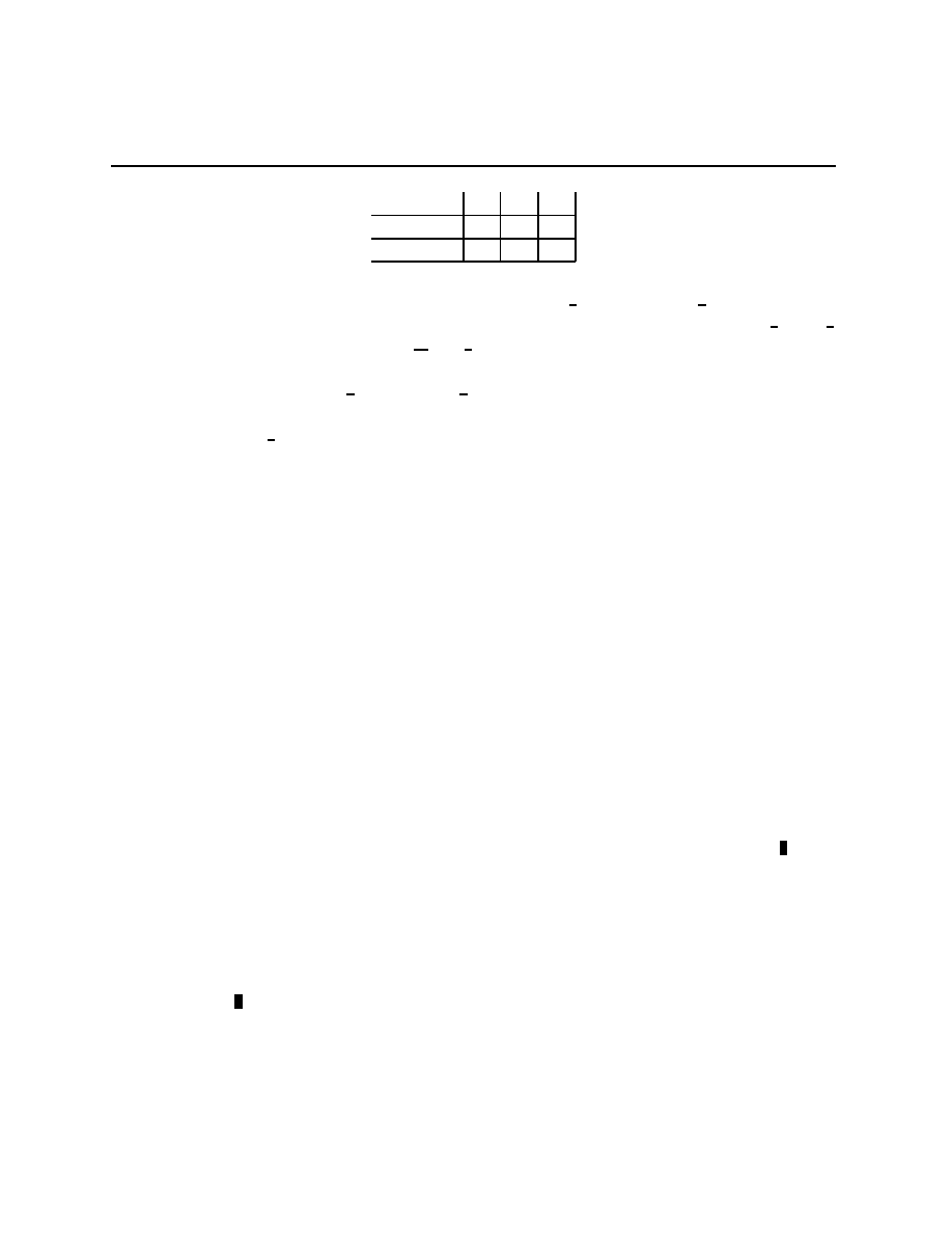
Example 1.2 (The value of information) Ω =

{L, M, R} with Q(L) = Q(M) =

and

Q(R) =

being the probability distribution on Ω. A =

{U, D}, and u(a, ω) is given in the

table

Chapter 1.3

↓, Ω →

Not being able to distinguish M from R is a situation of partial information. It can

be modelled with S =

{l, ¬l}, P ((l, L)) = P ((¬l, M) =

, P ((

¬l, R) =

. It’s clear that

∗

(l) = U and a

∗

(

¬l) = D. These give utilities of 10 and 8 with probabilities

and

respectively, for an expected utility of

= 8

Compare this with the full information case, which can be modelled with S =

{l, m, r}

and P ((l, L)) = P ((m, M ) =

, P ((r, R) =

. Here β

= δ

, β

= δ

, and β

= δ

(where

is point mass on x). Therefore, a

∗

(l) = U , a

∗

(m) = 8, and a

∗

(r) = U which gives an

expected utility of 9

1.2

The bridge crossing and rescaling Lemmas

We ended the examples by calculating some ex ante expected utilities under different plans.
Remember that optimal plans are defined by setting a

∗

(s) to be any of the solutions to the

problem

max

a∈A

u(a, ω)β

(ω).

These are plans that can be thought of as being formed after s is observed and beliefs β

have been formed, an “I’ll cross that bridge when I come to it” approach. There is another
way to understand the formation of these plans.

More notation: “iff” is read “if and only if.”

Lemma 1.3 (Bridge crossing) A plan a(

·) is optimal iff it solves the problem

max

a(·)∈A

S×Ω

u(a(s), ω) dP (s, ω).

Proof: Write down Bayes’ Law and do a little bit of re-arrangement of the sums.

In thinking about optimal plans, all that can conceivably matter is the part of the

utilities that is affected by actions. This seems trivial, but it will turn out to have major
implications for our interpretations of equilibria in game theory.

Lemma 1.4 (Rescaling)

∀a, b ∈ A, ∀P ∈ ∆(F),

Ω

u(a, ω) dP (ω)

≥

Ω

u(b, ω) dP (ω) iff

Ω

[α

· u(a, ω) + f(ω)] dP (ω) ≥

Ω

[α

· u(b, ω) + f(ω)] dP (ω) for all α > 0 and functions f.

Proof: Easy.

Remember how you learned that Bernoulli utility functions were immune to multiplica-

tion by a positive number and the addition of a constant? Here the constant is being played
by

Ω

(ω) dP (ω).

Chapter 1.3

1.3

Behavior

The story so far has the joint realization of s and ω distributed according to the prior
distribution P

∈ ∆(S × Ω), the observation of s, followed by the choice of a ∈ a

∗

(s). Note

that

∈ a

∗

(s) iff

∀b ∈ a

u(a, ω)β

(ω)

≥

u(b, ω)β

(ω).

(1.1)

(1.1) can be expressed as E

×β

≥ E

×β

u, which highlights the perspective that the

person is choosing between different distributions. Notice that if a, b

∈ a

∗

(s), then E

×β

u =

×β

u, and both are equal to E

(αδ

+(1−α)δ

)×β

u. In words, of both a and b are optimal,

then so is any distribution that puts mass α on a and (1

− α) on b. Said yet another way,

∆(a

∗

(s)) is the set of optimal probability distributions.

(1.1) can also be expressed as u

· β

≥ u

· β

where u

, u

, β

∈ R

Ω

, which highlights

the linear inequalities that must be satisfied by the beliefs. It also makes the shape of the
optimal distributions clear, if u

· β

= u

· β

= m, then for all α, [αu

+ (1

− α)u

]

· β

= m.

Thus, if play of either a or b is optimal, then playing a the proportion α of the time and
playing b the proportion 1

− α of the time is also optimal.

Changing perspective a little bit, regard S as the probability space, and a plan a(

·) ∈ A

as a random variable. Every random variable gives rise to an outcome, that is, to a
distribution Q on A. Let Q

∗

⊂ ∆(A) denote the set of outcomes that arise from optimal

plans for a given P . Varying P and looking at the set of Q

∗

’s that arise gives the set of

possible observable behaviors.

To be at all useful, this theory must rule out some kinds of behavior. At a very general

level, not much is ruled out.

An action a

∈ A is potentially Rational (pR ) if there exists some β

such that

∈ a

∗

(β

). An action a dominates action b if

∀ω u(a, ω) > u(b, ω). The following

example shows that an action b can be dominated by a random choice.

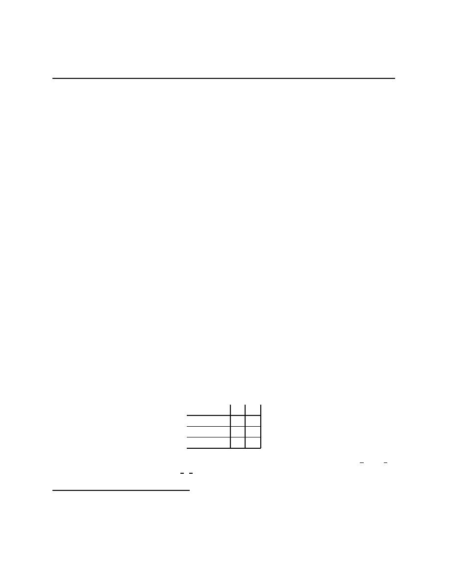
Example 1.5 Ω =

{L, R}, A = {a, b, c}, and u(a, ω) is given in the table

↓, Ω → L R

Whether or not a is better than c or vice versa depends on beliefs about ω, but

dominates b. Indeed, for all α

∈ (

), αδ

+ (1

− α)δ

dominates b.

I may slip and use the phrase “a mixture” for “a probability.” This is because there are (infinite)

contexts where one wants to distinguish between mixture spaces and spaces of probalities.

Chapter 1.4

As a point of notation, keeping the δ’s around for point masses is a bit of clutter we

can do without, so, when x and y are actions and α

∈ [0, 1], αx + (1 − α)y denotes the

probability that puts mass α on x and 1

− α on y. In the same vein, for σ ∈ ∆(A), we’ll

use u(σ, ω) for

u(a, ω)σ(a).

Definition 1.6 An action b is pure-strategy dominated if there exists a a

∈ A such

that for all ω, u(a, ω) > u(b, ω). An action b is dominated if there exists a σ

∈ ∆(A) such

that for all ω, u(σ, ω) > u(b, ω).

Lemma 1.7 a is pR iff a is not pure-strategy dominated, and every Q putting mass 1 on
the pR points is of the form Q

∗

for some P .

Proof: Easy.

Limiting the set of β

that are possible further restricts the set of actions that are pR.

In game theory, ω will contain the actions of other people, and we will derive restrictions
on β

from our assumption that they too are optimizing.

1.4

Problems

Problem 1.1 (Product spaces and product measures) X is the two point space

, x

Y is the three point space

, y

}, and Z is the four point space {z

, z

1. How many points are in the space X

× Y × Z?

2. How many points are in the set π

−1

3. How many points are in the set π

−1

4. How many points are in the set π

−1

5. Let E =

, y

} ⊂ Y . How many points are in the set π

−1

(E)?

6. Let F =

, z

} ⊂ Z. How many points are in the set π

−1

(E)

∩ π

−1

(F )? What

about the set π

−1

(E)

∪ π

−1

(F )?

7. Let P

(resp. P

, P

) be the uniform distribution on X (resp. Y , Z), and let Q =

× P

. Let G be the event that the random variables π

, π

, and π

have

the same index. What is Q(G)? Let H be the event that two or more of the random
variable have the same index. What is Q(H)?

Chapter 1.4

Problem 1.2 (The value of information) Fix a distribution Q

∈ ∆(Ω) with Q(ω) >

0 for all ω

∈ Ω. Let M

denote the set of signal structures P

∈ ∆(S × Ω) such that

marg

Ω

(P ) = Q. Signal structures are conditionally determinate if for all ω, P

= δ

for

some s

∈ S. (Remember, P

(A) = P (A

|π

−1

Ω

(ω)), so this is saying that for every ω there is

only one signal that will be given.) For each s

∈ S, let E

{ω ∈ Ω : P

= δ

1. For any conditionally determinate P , the collection

: s

∈ S} form a partition

of Ω. [When a statement is given in the Problems, your job is to determine whether
or not it is true, to prove that it’s true if it is, and to give a counter-example if it is
not. Some of the statements “If X then Y ” are not true, but become true if you add
interesting additional conditions, “If X and X

, then Y .” I’ll try to (remember to)

indicate which problems are so open-ended.]

2. For P, P

∈ M

, we define P

, read “P is at least as informative as P

,” if for all

utility functions (a, ω)

7→ u(a, ω), the maximal ex ante expected utility is higher under

P than it is under P

. As always, define

by P P

if P

and

¬(P

P ).

A partition

E is at least as fine as the partition E

if every E

∈ E

is the union

of elements of

Prove Blackwell’s Theorem (this is one of the many results with this name):

For conditionally determinate P, P

, P

iff

is at least as fine as

3. A signal space is rich if it has as many elements as Ω, written #S

≥ #Ω.

(a) For a rich signal space, give the set of P

∈ M

that are at least as informative

as all other P

∈ M

(b) (Optional) Repeat the previous problem for signal spaces that are not rich.

4. If #S

≥ 2, then for all q ∈ ∆(Ω), there is a signal structure P and an s ∈ S such that

= q. [In words, Q does not determine the set of possible posterior beliefs.]

5. With Ω =

{ω

, ω

}, Q = (

), and S =

{a, b}, find P, P

0 such that P P

Problem 1.3 Define a

b if a dominates b.

1. Give a reasonable definition of a

b, which would be read as “a weakly dominates b.”

2. Give a finite example of a choice problem where

is not complete.

3. Give an infinite example of a choice problem where for each action a there exists an

action b such that b

Chapter 1.4

4. Prove that in every finite choice problem, there is an undominated action. Is there

always a weakly undominated action?

Problem 1.4 We could have developed the theory of choice under uncertainty with signal
structures P

∈ ∆(S × Ω), utility functions v(a, s, ω), and with people solving the maximiza-

tion problem

max

a∈A

v(a, s, ω)β

(ω).

This seems more general since it allows utility to also depend on the signals.

Suppose we are given a problem where the utility function depends on s. We are going

to define a new, related problem in which the utility function does not depend on the state.

Define Ω

= S

× Ω and S

= S. Define P

, ω

) = P

, (s, ω)) =

P (s, ω) if s

= s

otherwise.

Define u(a, ω

) = u(a, (s, ω)) = v(a, s, ω).

Using the construction above, formalize and prove a result of the form “The extra gen-

erality in allowing utility to depend on signals is illusory.”

Problem 1.5 Prove Lemma 1.7.

Chapter 1.4

Chapter 2

Correlated Equilibria in Static Games

In this Chapter, we’re going to develop the parallels between the theory of choice under
uncertainty and game theory. We start with static games, dominant strategies, and then
proceed to rationalizable strategies and correlated equilibria.
Readings: In whatever text(s) you’ve chosen, look at the sections on static games, dominant
strategies, rationalizable strategies, and correlated equilibria.

2.1

Generalities about static games

One specifies a game by specifying who is playing, what actions they can take, and their
prefernces. The set of players is I, with typical members i, j. The actions that i

∈ I can

take, are A

. Preferences of the players are given by their von Neumann-Morgenstern (or

Bernoulli) utility functions u

(

·). In general, each player i’s well-being is affected by the

actions of players j

6= i. A vector of strategies a = (a

)

i∈I

lists what each player is doing,

the set of all such possible vectors of strategies is the set A =

i∈I

. We assume that i’s

preferences over what others are doing can be represented by a bounded utility function
u

: A

→ R. Summarizing, game Γ is a collection (A

, u

)

i∈I

. Γ is finite if A is.

The set A can be re-written as A

× A

I\{i}

, or, more compactly, as A

× A

−i

. Letting

Ω

= A

−i

, each i

∈ I faces the optimization problem

max

a∈A

, ω

)

where they do not know ω

. We assume that each i treats what others do as a (possibly

degenerate) random variable,

At the risk of becoming overly repetitious, the players, i

∈ I, want to pick that action

or strategy that maximizes u

. However, since u

may, and in the interesting cases, does,

depend on the choices of other players, this is a very different kind of maximization than is

Chapter 2.3

found in neoclassical microeconomics.

2.2

Dominant Strategies

In some games, some aspects of players’ preferences do not depend on what others are doing.
From the theory of choice under uncertainty, a probability σ

∈ ∆(A) dominates action

b if

∀ω u(σ, ω) > u(b, ω). In game theory, we have the same definition – the probability

∈ ∆(A

) dominates b

if,

∀ a

−i

∈ A

−i

, u

(σ

, a

−i

) > u

, a

−i

). The action b

being

dominated means that there are no beliefs about what others are doing that would make b

an optimal choice.

There is a weaker version of domination, σ

weakly dominates b

if,

∀ a

−i

∈ A

−i

(σ

, a

−i

)

≥ u

, a

−i

) and

∃a

−i

∈ A

−i

such that u

(σ

, a

−i

) > u

, a

−i

). This means that

is always at least as good as b

, and may be strictly better.

A strategy a

is dominant in a game Γ if for all b

, a

dominates b

, it is weakly

dominant if for all b

, a

weakly dominates b

2.3

Two classic games

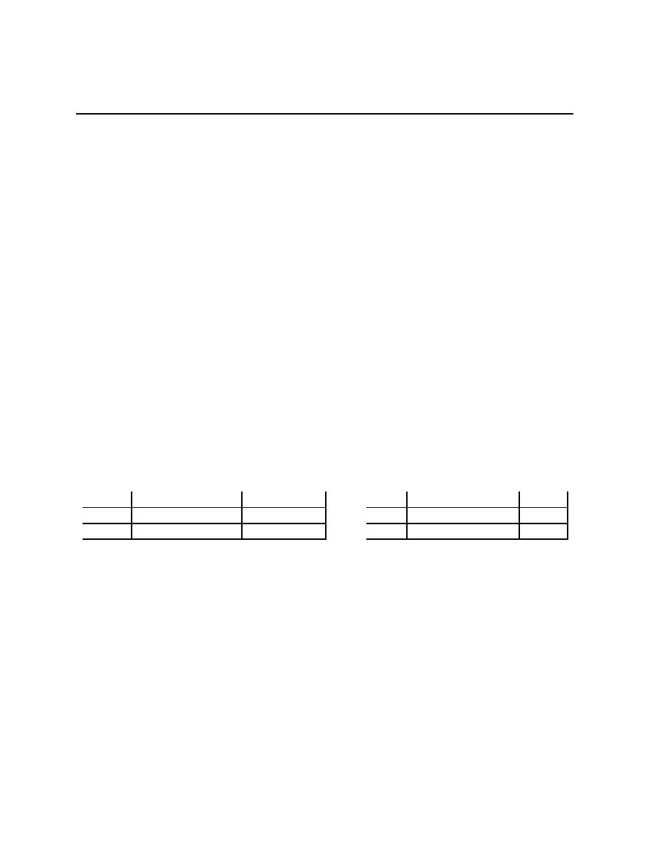
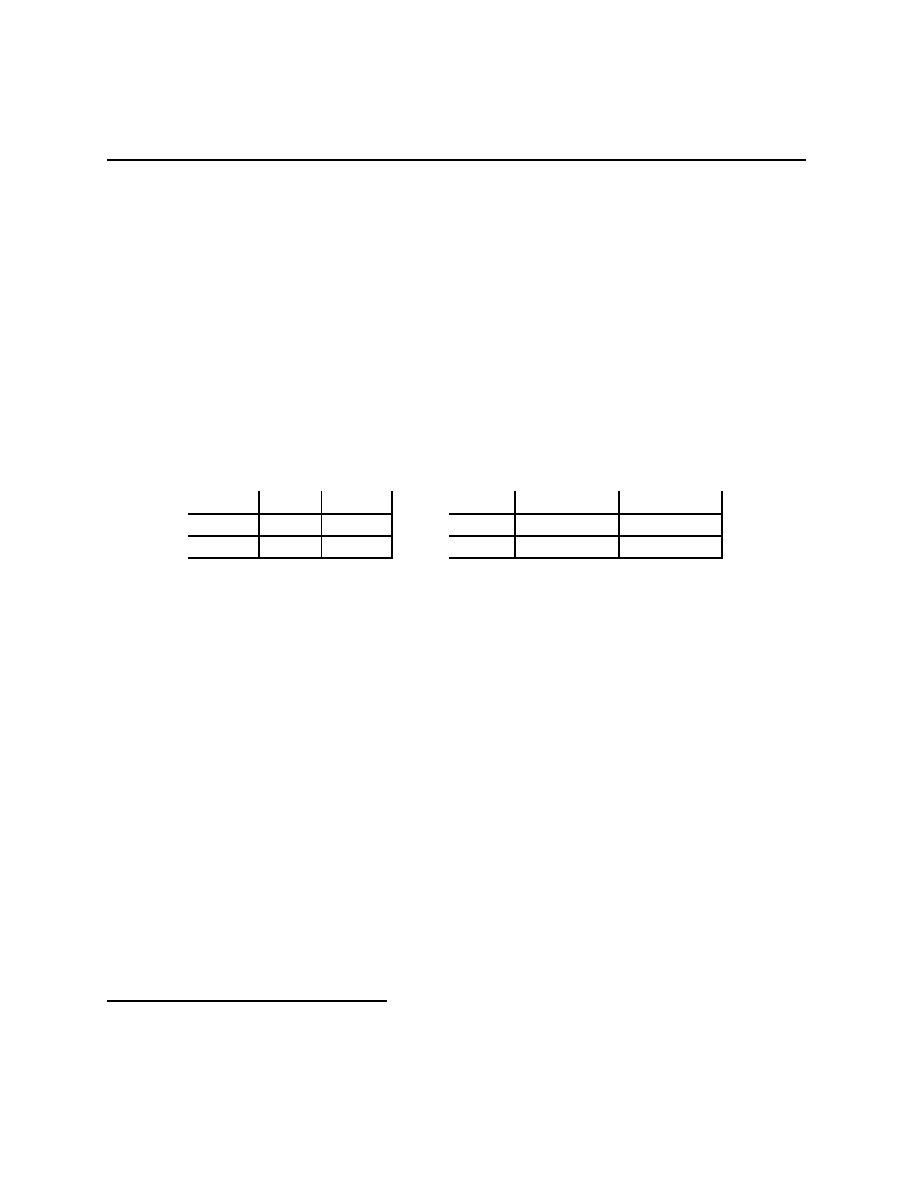
These two classic games have dominant strategies for at least one player.

Prisoners’ Dilemma

Rational Pigs

Squeal

Silent

Squeal

(

−B + r, −B + r) (−b + r, −B)

Silent

(

−B, −b + r)

(

−b, −b)

Push

Wait

Push

(

−c + e, b − e − c) (−c, b)

Wait

(αb, (1

− α)b − c)

(0, 0)

Both of these games are called 2

×2 games because there are two players and each player

has two actions. For the first game, A

{Squeal

, Silent

} and A

{Squeal

, Silent

Some conventions: The representation of the choices has player 1 choosing which row

occurs and player 2 choosing which column; If common usage gives the same name to actions
taken by different players, then we do not distinguish between the actions with the same
name; each entry in the matrix is uniquely identified by the actions a

and a

of the two

players, each has two numbers, (x, y), these are (u

, a

), u

, a

)), so that x is the utility

of player 1 and y the utility of player 2 when the vector a = (a

, a

) is chosen.

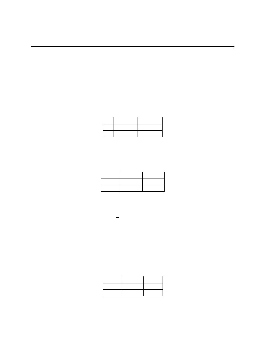
There are stories behind both games. In the first, two criminals have been caught, but it

is after they have destroyed the evidence of serious wrongdoing. Without further evidence,
the prosecuting attorney can charge them both for an offense carrying a term of b > 0
years. However, if the prosecuting attorney gets either prisoner to give evidence on the

Chapter 2.3

other (Squeal), they will get a term of B > b years. The prosecuting attorney makes a
deal with the judge to reduce any term given to a prisoner who squeals by an amount r,
b

≥ r > 0, B − b > r (equivalent to −b > −B + r). With B = 15, b = r = 1, this gives

Squeal

Silent

Squeal

(

−14, −14) (0, −15)

Silent

(

−15, 0)

(

−1, −1)

In the second game, there are two pigs, one big and one little, and each has two actions.

Little pig is player 1, Big pig player 2, the convention has 1’s options being the rows, 2’s the
columms, payoffs (x, y) mean “x to 1, y to 2.” The story is of two pigs in a long room, a
lever at one end, when pushed, gives food at the other end, the Big pig can move the Little
pig out of the way and take all the food if they are both at the food output together, the
two pigs are equally fast getting across the room, but when they both rush, some of the
food, e, is pushed out of the trough and onto the floor where the Little Pig can eat it, and
during the time that it takes the Big pig to cross the room, the Little pig can eat α of the
food. This story is interesting when b > c

− e > 0, c > e > 0, 0 < α < 1, (1 − α)b − c > 0.

We think of b as the benefit of eating, c as the cost of pushing the lever and crossing the
room. With b = 6, c = 1, e = 0.1, and α =

, this gives

Push

Wait

Push

(

−0.9, 4.9) (−1, 6)

Wait

(3, 2)

(0, 0)

In the Prisoners’ Dilemma, Squeal dominates Silent for both players. Another way to

put this, the only pR action for either player is Squeal. In the language developed above,
the only possible outcome for either player puts probability 1 on the action a

= Squeal. We

might as well solve the optimization problems independently of each other. What makes it
interesting is that when you put the two solutions together, you have a disaster from the
point of view of the players. They are both spending 14 years in prison, and by cooperating
with each other and being Silent, they could both spend only 1 year in prison.

I first read this in [5].

One useful way to view many economists is as apologists for the inequities of a moderately classist

version of the political system called laissez faire capitalism. Perhaps this is the driving force behind the
large literature trying to explain why we should expect cooperation in this situation. After all, if economists’
models come to the conclusion that equilibria without outside intervention can be quite bad for all involved,
they become an attack on the justifications for laissez faire capitalism. Another way to understand this
literature is that we are, in many ways, a cooperative species, so a model predicting extremely harmful
non-cooperation is very counter-intuitive.

Chapter 2.4

In Rational Pigs, Wait dominates Push for the Little Pig, so Wait is the only pR for 1.

Both Wait and Push are pR for the Big Pig, and the set of possible outcomes for Big Pig
is ∆(A

). If we were to put these two outcomes together, we’d get the set δ

Wait

× ∆(A

(New notation there, you can figure out what it means.) However, some of those outcomes
are inconsistent.

Wait is pR for Big Pig, but it optimal only for beliefs β putting mass of at least

the Little Pig Push’ing (you should do that algebra). But the Little Pig never Pushes.
Therefore, the only beliefs for the Big Pig that are consistent with the Little Pig optimizing
involve putting mass of at most 0 in the Little Pig pushing. This then reduces the outcome
set to (Wait, Push), and the Little Pig makes out like a bandit.

2.4

Signals and Rationalizability

Games are models of strategic behavior. We believe that the people being modeled have
all kinds of information about the world, and about the strategic situation they are in.
Fortunately, at this level of abstraction, we need not be at all specific about what they
know beyond the assumption that player i’s information is encoded in a signal s

taking its

values in some set S

. If you want to think of S

as containing a complete description of the

physical/electrical state of i’s brain, you can, but that’s going further than I’m comfortable.
After all, we need a tractable model of behavior.

Let R

= pR

⊂ A

denote the set of potentially rational actions for i. Define R

i∈I

so that ∆(R

) is the largest possible set of outcomes that are at all consistent with

rationality. (In Rational Pigs, this is the set δ

Wait

× ∆(A

).) As we argued above, it is too

large a set. Now we’ll start to whittle it down.

Define R

to be the set of maximizers for i when i’s beliefs β

have the property that

(

j6=i

) = 1. Since R

is the set of maximizers against a smaller set of possible beliefs,

⊂ R

. Define R

i∈I

, so that ∆(R

) is a candidate for the set of outcomes

consistent with rationality. (In Rational Pigs, this set is

{δ

(Wait, Push)

}).

Given R

has been define, inductively, define R

n+1

to be the set of maximizers for i

when i’s beliefs β

have the property that β

(

j6=i

) = 1. Since R

is the set of maximizers

against a smaller set of possible beliefs, R

n+1

⊂ R

. Define R

n+1

i∈I

n+1

, so that

∆(R

) is a candidate for the set of outcomes consistent with rationality.

Lemma 2.1 For finite games,

∃N∀n ≥ N R

= R

We call R

∞

n∈N

the set of rationalizable strategies. ∆(R

∞

) is then the set

See the NYT article about brain blood flow during play of the repeated Prisoners’ Dilemma.

Chapter 2.5

of signal rationalizable outcomes.

There is (at least) one odd thing to note about ∆(R

∞

) — suppose the game has more

than one player, player i can be optimizing given their beliefs about what player j

6= i is

doing, so long as the beliefs put mass 1 on R

∞

. There is no assumption that this is actually

what j is doing. In Rational Pigs, this was not an issue because R

∞

had only one point,

and there is only one probability on a one point space. The next pair of games illustrate
the problem.

2.5

Two classic coordination games

These two games have no dominant strategies for either player.

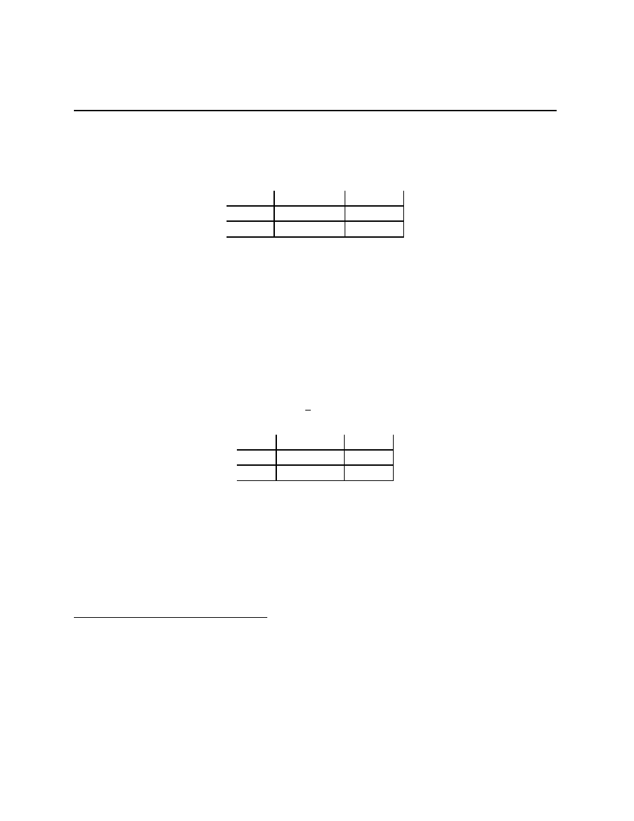
Stag Hunt

Battle of the Partners

Stag

Rabbit

Stag

(S, S)

(0, R)

Rabbit

(R, 0)

(R, R)

Dance

Picnic

Dance

(F + B, B)

(F, F )

Picnic

(0, 0)

(B, F + B)

As before, there are stories for these games. For the Stag Hunt, there are two hunters

who live in villages at some distance from each other in the era before telephones. They need
to decide whether to hunt for Stag or for Rabbit. Hunting a stag requires that both hunters
have their stag equipment with them, and one hunter with stag equipment will not catch
anything. Hunting for rabbits requires only one hunter with rabbit hunting equipment. The
payoffs have S > R > 0. This game is a coordination game, if the players’ coordinate
their actions they can both achieve higher payoffs. There is a role then, for some agent to
act as a coordinator. Sometimes we might imagine a tradition that serves as coordinator —
something like we hunt stags on days following full moons except during the spring time.
Macroeconomists, well, some macroeconomists anyway, tell stories like this but use the code
word “sunspots” to talk about coordination. Any signals that are correlated and observed
by the agents can serve to coordinate their actions.

The story for the Battle of the Partners game involves two partners who are either going

to the (loud) Dance club or to a (quiet) romantic evening Picnic on Friday after work.
Unfortunately, they work at different ends of town and their cell phones have broken so
they cannot talk about which they are going to do. Each faces the decision of whether to
drive to the Dance club or to the Picnic spot not knowing what the other is going to do.
The payoffs have B

F > 0 (the “” arises because I am a romantic). The idea is that

I say “signal rationalizable” advisedly. Rationalizable outcomes involve play of rationalizable strate-

gies, just as above, but the randomization by the players is assumed to be stochastically independent.

Chapter 2.6

the two derive utility B from Being together, utility F from their Favorite activity, and that
utilities are additive.

For both of these games, A = R

= R

· · · = R

= R

n+1

· · ·. Therefore, ∆(A)

is the set of signal rationalizable outcomes. Included in ∆(A) are the point masses on the
off-diagonal actions. These do not seem sensible. They involve both players taking an action
that is optimal only if they believe something that is not true.

2.6

Signals and Correlated Equilibria

We objected to anything other than (Wait, Push) in Rational Pigs because anything other
than (Wait, Push) being an optimum involved Big Pig thinking that Little Pig was doing
something other than what he was doing. This was captured by rationalizability for the
game Rational Pigs. As we just saw, rationalizability does not capture everything about
this objection for all games. That’s the aim of this section.

When i sees s

and forms beliefs β

, β

should be the “true” distribution over what the

player(s) j

6= i is(are) doing, and what they are doing should be optimal for them. The way

that we get at these two simultaneous requirements is to start by the observation that there
is some true P

∈ ∆(S × A). Then all we need to do is to write down (and interpret) two

conditions:

1. each β

is the correct conditional distribution, and

2. everyone is optimizing given their beliefs.

2.6.1

The common prior assumption

A system of beliefs is a set of mappings, one for each i

∈ I, s

7→ β

, from S

to ∆(A

−i

If we have a marginal distribution, Q

, for the s

, then, by Bayes’ Law, any belief system

arises from the distribution P

∈ ∆(S

×A

−i

) defined by P

(B) =

(B)

· Q

). In this

sense, i’s beliefs are generated by P

. For each player’s belief system to be correct requires

that it be generated by the true distribution.

Definition 2.2 A system of beliefs s

7→ β

, i

∈ I, is generated by P ∈ ∆(S × A) if

∀i ∈ I ∀s

∈ S

∀E

−i

⊂ A

−i

) = P (π

−1

−i

)

|π

−1

)).

(2.1)

A system of beliefs has the common prior property if it is generated by some P

∈

∆(S

× A).

On the left-hand side of the equality in (2.1) are i’s beliefs after seeing s

. As we have

seen (Problem 1.2.4), without restrictions on P , β

can be any probability on A

−i

. We

Chapter 2.6

now limit that freedom by an assumption that we will maintain whenever we are analyzing
a strategic situation.

Assumption 2.3 Beliefs have the common prior property.

The restriction is that there is a single, common P that gives everyone’s beliefs when

they condition on their signals. Put in slightly different words, the prior distribution is
common amongst the people involved in the strategic situation. Everyone understands the
probabilistic structure of what is going on.

It’s worth being very explicit about the conditional probability on the right-hand side

of (2.1). Define F = π

−1

−i

) = S

× A

× E

−i

, and G = π

−1

) =

} × S

−i

× A, so that

∩ G = {s

} × S

−i

× A

× E

−i

. Therefore,

P (F

|G) = P (π

−1

−i

)

|π

−1

)) =

P (

} × S

−i

× A

× E

−i

)

P (

} × S

−i

× A

−i

)

It’s important to note that β

contains no information about S

−i

, only about A

−i

, what

i thinks that

−i is doing. It is also important to note that conditional probabilities are not

defined when the denominator is 0, so beliefs are not at all pinned down at s

’s that have

probability 0. From a classical optimization point of view, that is because actions taken
after impossible events have no implications. In dynamic games, people decide whether or
not to make a decision based on what they think others’ reactions will be. Others’ reactions
to a choice may make it that choice a bad idea, in which case the choice will not be made.
But then you are calculating based on their reactions to a choice that will not happen, that
is, you are calculating based on others’ reactions to a probability 0 event.

2.6.2

The optimization assumption

Conditioning on s

gives beliefs β

. Conditioning on s

also gives information about A

what i is doing. One calls the distribution over A

i’s strategy. The distribution on A

that is, the strategy, should be optimal from i’s point of view.

A strategy σ is a set of mappings, one for each i

∈ I, s

7→ σ

, from S

to ∆(A

). σ is

optimal for the beliefs s

7→ β

, i

∈ I if for all i ∈ I, σ

∗

(β

)) = 1.

Definition 2.4 A strategy s

7→ σ

, i

∈ I, is generated by P ∈ ∆(S × A) if

∀i ∈ I ∀s

∈ S

∀E

⊂ A

) = P (π

−1

)

|π

−1

)).

(2.2)

A P

∈ ∆(S × A) has the (Bayesian) optimality property if the strategy it generates is

optimal for the belief system it generates.

Chapter 2.6

2.6.3

Correlated equilibria

The roots of the word “equilibrium” are “equal” and “weight,” the appropriate image is
of a pole scale, which reaches equilibrium when the weights on both sides are equal. That
is, following the Merriam-Webster dictionary, a state of balance between opposing forces or
actions that is static (as in a body acted on by forces whose resultant is zero).

If a distribution P

∈ ∆(S × A) satisfies Bayesian optimality, then none of the people

involved have an incentive to change what they’re doing. Here we are thinking of peoples’
desires to play better strategies as a force pushing on the probabilities. The system of forces
is in equilibrium when all of the forces are 0 or up against the boundary of the space of
probabilities.

One problem with looking for P that satisfy the Bayesian optimality property is that

we haven’t specified the signals S =

i∈I

. Indeed, they were not part of the description

of a game, and I’ve been quite vague about them. This vagueness was on purpose. I’m now
going to make them disappear in two different ways.

Definition 2.5 A µ

∈ ∆(A) is a correlated equilibrium if there exists a signal space

S =

i∈I

and a P

∈ ∆(S × A) having the Bayesian optimality property such that µ =

marg

(P ).

This piece of sneakiness means that no particular signal space enters. The reason that

this is a good definition can be seen in the proof of the following Lemma. Remember that
µ

∈ ∆(A) is a vector in R

such that

µ(a) = 1.

Lemma 2.6 µ

∈ ∆(A) is a correlated equilibrium iff

∀i ∈ I ∀a

, b

∈ A

−i

, a

−i

)µ(a

, a

−i

)

≥

−i

, a

−i

)µ(a

, a

−i

Proof: Not easy, using the A

as the canonical signal spaces.

What the construction in the proof tells us is that we can always take S

= A

, and have

the signal “tell” the player what to do, or maybe “suggest” to the player what to do. This
is a very helpful fiction for remembering how to easily define and check that a distribution
µ is a correlated equilibrium. Personally, I find it a bit too slick. I’d rather imagine there
is some complicated world out there generating random signals, that people are doing the
best they can from the information they have, and that an equilibrium is a probabilistic
description of a situation in which people have no incentive to change what they’re doing.

There are also “dynamic” equilibria as in a reversible chemical reaction when the rates of reaction in

both directions are equal. We will see these when we look at evolutionary arguments later.

Chapter 2.8

2.6.4

Existence

There is some question about whether all of these linear inequalities can be simultaneously
satisfied. We will see below that every finite game has a Nash equilibrium. A Nash equilib-
rium is a correlated equilibrium with stochastically independent signals. That implies that
the set of correlated equilibria is not empty, so correlated equilibria exist. That’s fancy and
hard, and relies on a result called a fixed point theorem. There is a simpler way.

The set of correlated equilibria is the set µ that satisfy a finite collection of linear

inequalities. This suggests that it may be possible to express the set of correlated equilibria
as the solutions to a linear programming problem, one that we know has a solution. This
can be done.

Details here (depending on time).

2.7

Rescaling and equilibrium

One of the important results in the theory of choice under uncertainty is Lemma 1.4. It says
that the problem max

a∈A

u(a, ω) dβ

(ω) is the same as the problem max

a∈A

[αu(a, ω) +

f (ω)] dβ

(ω) for all α > 0 and functions f that do not depend on a. Now ω is being identified

with the actions of others. The Lemma still holds.

Fix a finite game Γ(u) = (A

, u

)

i∈I

. For each i

∈ I, let α

> 0, let f

: A

−i

→ R, and

define v

= α

· u

+ f

so that Γ(v) = (A

, α

· u

+ f

)

i∈I

Lemma 2.7 CEq(Γ(u)) = CEq(Γ(v)).

Proof: µ

∈ CEq(Γ(u)) iff ∀i ∈ I ∀a

, b

∈ A

−i

, a

−i

)µ(a

, a

−i

)

≥

−i

, a

−i

)µ(a

, a

−i

(2.3)

Similarly, µ

∈ CEq(Γ(v)) iff ∀i ∈ I ∀a

, b

∈ A

−i

[α

, a

−i

) + f

−i

)]µ(a

, a

−i

)

≥

−i

[α

, a

−i

) + f

−i

)]µ(a

, a

−i

(2.4)

Since α

> 0, (2.3) holds iff (2.4) holds.

Remember how you learned that Bernoulli utility functions were immune to multiplica-

tion by a positive number and the addition of a constant? Here the constant is being played
by

−i

) dβ

−i

Chapter 2.8

2.8

How correlated equilibria might arise

There are several adaptive procedures that converge to the set of equilibria for every finite
game. The simplest is due to Hart and Mas-Colell (E’trica 68 (5) 1127-1150). They give an
informal description of the procedure:

Player i starts from a “reference point”: his current actual play. His choice next
peried is govered by propensities to depart from it. . . . if a change occurs, it
should be to actions that are perceived as being better, relative to the current
choice. In addition, and in the spirit of adaptive behavior, we assume that
all such better choices get positive probabilities; also, the better an alternative
action seems, the higher the probability of choosing it next time. Further, there
is also inertia: the probability of staying put (and playing the same action as in
the last period) is always positive.

The idea is that players simultaneously choose actions a

i,t

at each time t, t = 1, 2, . . ..

After all have made a choice, each i

∈ I learns the choices of the others and receives their

payoff, u

i,t

), a

= (a

i,t

, a

−i,t

). They then repeat this procedure. Suppose that h

= (a

)

τ =1

has been played. At time t + 1 each player picks an action a

i,t+1

according to a probability

distribution p

i,t+1

which is defined in a couple of steps. We assume that the choices are

independent across periods.

1. For every a

6= b in A

and τ

≤ t, define

i,τ

(a, b) =

(b, a

−i,τ

) if a

i,t

= a

)

otherwise.

This gives the stream of payoffs that would have arisen if b were substituted for a at
each point in the past where a was played.

2. Define the average difference as

i,t

(a, b) =

τ ≤t

i,τ

(a, b)

−

τ ≤t

i,τ

3. Define the average regret at time t for not having played b instead of a by

i,t

(a, b) = max

i,t

(a, b), 0

Chapter 2.9

4. For each i

∈ I, fix a moderately large µ (see below), and suppose that a was played

at time t. Then p

i,t+1

is defined as

i,t+1

(b) =

i,t

(a, b)

for all b

6= a

i,t+1

(a) = 1

−

b6=a

i,t+1

(b)

The detail about µ

— pick it sufficiently large that p

i,t+1

(a) > 0.

An infinite length history h is a sequence (a

)

∞

τ =1

. For each h, define µ

t,h

as the empirical

distribution of play after t periods, along history h, that is, µ

t,h

(a) =

{τ ≤ t : a

= a

Theorem 2.8 If players start arbitrarily for any finite number of periods, and then play ac-
cording to the procedure just outlined, then for every h in a set of histories having probability
1, d(µ

t,h

, CEq)

→ 0 where CEq is the set of correlated equilibria.

Proof: Not at all easy.

This procedure has no “strategic reasoning” feel to it. The players calculate which action

is better by looking at their average regret for not having played an action in the past. That
is, they look through the past history, and everywhere they played action a, they consider
what their payoffs would have happened if they had instead played action b. This regret is
calculated without thinking about how others might have reacted to the change from a to
b. In other words, this procedure gives a simple model of behavior that leads to what looks
like a very sophisticated understanding of the strategic situation.

A final pair of notes: (1) It is possible to get the same kind of convergence even if the

people do not observe what the others are doing. What one does is to estimate the regret
statistically. This is (a good bit) more difficult, but it is reassuring that people can “learn”
their way to an equilibrium even without knowing what everyone else is up to. (2) The
dynamic is almost unchanged if we rescale using Lemma 2.7, that is, changing u

(a) to

(a) + f

−i

). I say almost because the µ

and α

can substitute for each other — look

at the definition of D

i,t

(a, b), the f

−i

) part disappears, but the α

comes through, giving

the p

i,t

multiplier.

2.9

Problems

The results of problems with

∗

’s before them will be used later.

Problem 2.1 For every N

∈ N, there is a finite game such that R

( R

n−1

for all 2

≤

≤ N, and R

= R

for all n

≥ N.

Chapter 2.9

Problem 2.2 Find the set of correlated equilibria for the Prisoners’ Dilemma and for Ra-
tional Pigs. Prove your answers (i.e. write out the inequalities that must be satisfied and
show that you’ve found all of the solutions to these inequalities).

∗

Problem 2.3 Two players have identical gold coins with a Heads and a T ails side. They

simultaneously reveal either H or T . If the gold coins match, player 1 takes both, if they
mismatch, player 2 takes both. This is called a 0-sum game because the sum of the winnings
of the two players in this interaction is 0. The game is called “Matching Coins” (“Matching
Pennies” historically), and has the matrix representation

(+1,

−1) (−1, +1)

(

−1, +1) (+1, −1)

Find the set of correlated equilibria for this game, proving your answer.

∗

Problem 2.4 Take B = 10, F = 2 in the Battle of the Partners game so that the payoff

matrix is

Dance

Picnic

Dance

(12, 10)

(2, 2)

Picnic

(0, 0)

(10, 12)

1. Explicitly give all of the inequalities that must be satisfied by a correlated equilibrium.

2. Show that the µ putting mass

each on (Dance, Dance) and (Picnic, Picnic) is a

correlated equilibrium.

3. Find the set of correlated equilibria with stochastically independent signals.

4. Find the maximum probability that the Partners do not meet each other, that is, maxi-

mize µ(Dance, Picnic)+µ(Picnic, Dance) subject to the constraint that µ be a correlated
equilibrium.

∗

Problem 2.5 Take S = 10 and R = 1 in the Stag Hunt game so that the payoff matrix is

Stag

Rabbit

Stag

(10, 10)

(0, 1)

Rabbit

(1, 0)

(1, 1)

Chapter 2.9

1. Explicitly give all of the inequalities that must be satisfied by a correlated equilibrium.

2. Find the set of correlated equilibria with stochastically independent signals.

3. Give three different correlated equilibria in which the hunters’ actions are not stochas-

tically independent.

4. Find the maximum probability that one or the other hunter goes home with nothing.

∗

Problem 2.6 Apply Lemma 2.7 to the numerical versions of the Prisoners’ Dilemma,

Rational Pigs, Battle of the Partners, and the Stag Hunt given above so as to find games
with the same set of equilibria and having (0, 0) as the off-diagonal utilities.

Problem 2.7 (Requires real analysis) For all infinite length histories h, d(µ

t,h

, CEq)

→

0 iff for all i

∈ I and all a 6= b ∈ A

, R

i,t

(a, b)

→ 0. In words, regrets converging to 0 is the

same as the empirical distribution converging to the set of correlated equilibria.

Chapter 2.9

Chapter 3

Nash Equilibria in Static Games

A Nash equilibrium is a special kind of correlated equilibrium, it is the single most used solu-
tion concept presently used in economics. The examples are the main point of this chapter.
They cover a range of the situations studied by economists that I’ve found interesting, or
striking, or informative. Hopefully, study of the examples will lead to broad, generalizable
skills in analysis in the style of modern economics.

3.1

Nash equilibria are uncorrelated equilibria

A solution concept is a mapping from games Γ = (A

, u

)

i∈I

, to sets of outcomes, that

is, to subsets of ∆(A). The previous chapter dealt with the solution concept “correlated
equilibrium,” CEq(Γ)

⊂ ∆(A) being defined by a finite set of inequalities.

A correlated equilibrium is a Nash equilibrium if the signals s

are stochastically

independent. Thus, all Nash equilibria are correlated equilibria, but the reverse is not true.
This solution concept is so now so prevalent in economics that the name “Nash” is often
omitted, and we’ll feel free to omit it too, as in Eq(Γ) being the set of equilibria from the
game Γ.

Remember that functions of independent random variables are themselves indepen-

dent. Therefore, a Nash equilibrium, µ

∈ ∆(A), is a correlated equilibrium having µ =

i∈I

marg

(µ). This implies that, if we were to pay attention to the signals in the canonical

version of the correlated equilibrium, β

would always be equal to

j6=i

. From this and

the optimality condition of correlated equilibria, we have

Lemma 3.1 µ

∈ Eq(Γ) iff µ = ×

i∈I

marg

(µ) and

∀i ∈ I µ

∗

(

j6=i

marg

(µ))) = 1.

In a 2

× 2 example where A

{T, B} (top and bottom) and A

{L, R} (left and

right), if µ

= (1/3, 2/3) and µ

= (3/4, 1/4) then µ = (µ

, µ

) denotes the probability

distribution

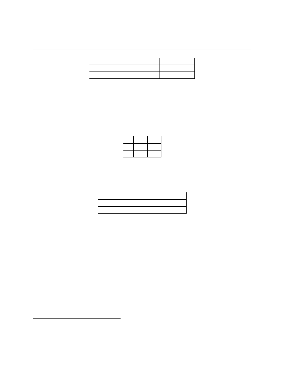
Chapter 3.1

(L) = 3/4

(R) = 1/4

(T ) = 1/3

1/4

1/12

(B) = 2/3

1/2

1/6

The marginal distributions are µ

and µ

, and for any a = (a

, a

)

∈ A, µ(a) = µ

)

·µ

Yet another way to look at what is happening is to say that if we pick a

∈ A according to

µ, then the random variables π

(a) = a

are stochastically independent.

Just as not all collections of random variables are independent, not all distributions on

A are product distributions. For example, the following distribution has strong correlation
between the two players’ choices,

1/4

3/4

Pure strategies are simply special cases of mixed strategies, cases in which for each i

∈ I,

each a

∈ A

, µ

) is equal either to 0 or to 1. If µ

= (0, 1) and µ

= (1, 0) in a 2

× 2

example, then µ is the distribution

(L) = 1

(R) = 0

(T ) = 0

(B) = 1

We will give a proof of the following result later.

Theorem 3.2 (Nash) If Γ is finite, then Eq(Γ) is a closed, non-empty subset of ∆(A).

Corollary 3.3 If Γ is finite, then CEq(Γ) is a closed, non-empty, convex polytope in ∆(A).

Corollary 3.4 If #CEq(Γ) = 1, then CEq(Γ) = Eq(Γ).

A pure strategy equilibrium is an equilibrium

with µ

= δ

for some a

∈ A

for each

∈ I. This would be point mass on a vector a = (a

)

i∈I

with the property that a

∈ a

∗

−i

Notation: For a vector b

∈ A and a

∈ A

, we define

= (b

, . . . , b

i−1

, a

, b

i+1

, . . . , b

Note how I’ve already dropped the ‘Nash’ in “Nash equilibrium?”

Chapter 3.2

We will sometimes use this notation, and sometimes use the notation (a

, b

−i

). For a

∈ A,

define

(b) = arg maxu

\·) = {a

∈ A

: (

∀t

∈ A

)[u

)

≥ u

)]

“Br

(b)” is read as “i’s set of pure strategy best responses to b.” This is the same as a

∗

−i

Notice the redundancy built into this new notation.

∗

= (a

∗

)

i∈I

is a pure strategy equilibrium for Γ iff

(

∀i ∈ I)(∀a

∈ A

)[u

∗

)

≥ u

∗

)].

The set of pure strategy equilibria for Γ is denoted Eq

(Γ).

Think of a µ

∈ ∆(A) that is not an equilibrium. The definition implies

(

∃i ∈ I)(∃a

∈ A

)[u

(µ

) > u

(µ)].

In other words, at a non-equilibrium µ, at least one of the players has an incentive to change
her action. This makes the definition of equilibrium seem like a minimal kind of idea.

Equilibrium is a minimal kind of answer to the question, “Where might best responses

dynamics stay put?” It is a very strong kind of answer to the question, “What do we expect
to happen?” We saw a kind of dynamic system that settles down to the set of correlated
equilibria. We will come back to the question of what kinds of dynamics settle down to
Nash equilibria later, and perhaps we will like Nash equilibria better for that reason. For
right now, let us examine why equilibrium is much too strong an assumption.

Lemma 3.5 µ

∈ Eq(Γ) if and only if ∀i ∈ I µ

(Br

(µ)) = 1.

In other words, any convincing arguments for i playing µ

involve i acting as if they are

solving the problem

max

∈A

(µ

that is, acting as if they know that everyone else is playing their part of the vector µ, and
that they solve the implied maximization problem, and if there are many pure strategy
solutions to their problem, they are randomizing over these strategies in the correct fashion.

Part of the function of this course is to remove your resistance to the assumption that

equilibrium is descriptive of behavior. Some examples showing that we can tell a wonderful
variety of stories will help in this project.

I will take you to the top of the mountain and show you the wonders of games in economic theory. They

can be yours, if only you will promise yourself to equilibrium.

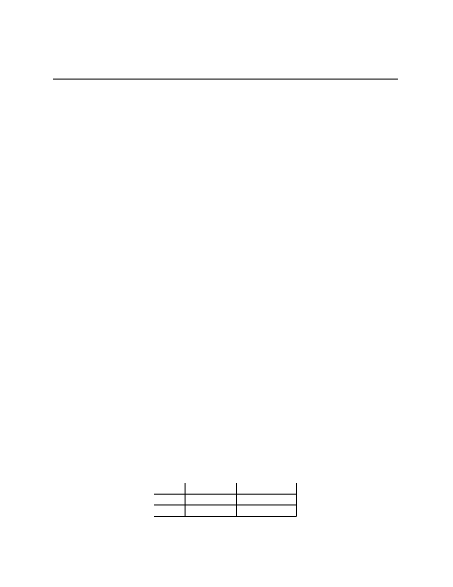
Chapter 3.2

3.2

2 × 2 games

We are going to focus on games where there are no ties — for each i

∈ I and a

−i

, u

, a

−i

)

, a

−i

) for a

6= b

. Within this class of 2

× 2 games, we’ve seen four types:

1. Games in which both players have a dominant strategy, e.g. Prisoners’ Dilemma;

2. Games in which exactly one player has a dominant strategy, e.g. Rational Pigs;

3. Games in which neither player has a dominant strategy and there are three equilibria,

e.g. Stag Hunt and Battle of the Partners;

4. Games in which neither player has a dominant strategy and there is only a mixed

strategy equilibrium, e.g. Matching Pennies.

We’re going to give three more stories for 2

×2 games, and see that they each fit into one

of the categories above. We’ll then use Lemma 1.4 and a definition of strategically equivalent
games to partition the set of all 2

× 2 games (with no ties) into these four categories. In the

process, we’ll see that Pareto rankings of equilibria mean less than we might have hoped.

3.2.1

Three more stories

There are Inspection games, games of Chicken, and Hawk-Dove conflicts. All of them fit
into one of the four categories above.

Inspection games

The idea in inspection games is that keeping someone honest is costly, so you don’t want
to spend effort monitoring their behavior. But if you don’t monitor their behavior, they’ll
want to slack off. The mixed strategy equilibria that we find balance these forces. We’ll
give two versions of this game, a very basic one, and a more complicated one.

The basic version: In this game, there is a worker who can either Shirk, or put in an

Effort. The boss can either inspect or not. Inspecting someone who is working has an
opportunity cost, c > 0, finding a Shirker has a benefit b. The worker receives w if they
Shirk and are not found out, 0 if they Shirk and are Inspected, and w

− e if they put in the

effort, whether or not they are Inspected. We assume that w > e > 0 so that w

− e > 0. In

matrix form, the game is

Inspect

Don’t inspect

Shirk

(0, b)

(w, 0)

Effort

− e, −c)

− e, 0)

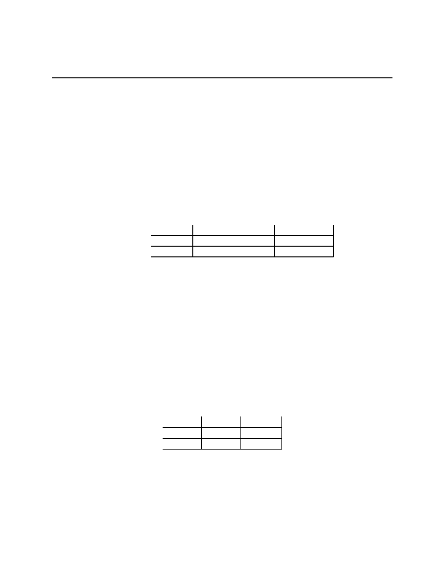
Chapter 3.2

Neither player has a dominant strategy, find the unique correlated equilibrium. This

game fits into the same category as Matching Coins.

Another, more heavily parametrized version: If a chicken packing firm leaves the fire

escape doors operable, they will lose c in chickens that disappear to the families and friends
of the chicken packers. If they nail or bolt the doors shut, which is highly illegal, they will
no longer lose the c, but, if they are inspected (by say OSHA), they will be fined f . Further,
if the firedoor is locked, there is a risk, ρ, that they will face civil fines or criminal worth
F if there is a fire in the plant that kills many of the workers because they cannot escape.

Inspecting a plant costs the inspectors k, not inspecting an unsafe plant costs B in terms
of damage done to the inspectors’ reputations and careers. Filling in the other terms, we
get the game

Inspectors

Inspect

Not inspect

Imperial

unlocked

(π

− c, −k)

(π

− c, 0)

locked

(π

− f − ρF, f − k) (π − ρF, −B)

If f and ρF are too low, specifically, if c > f + ρF , then Imperial has a dominant

strategy, and the game is, strategically, another version of Rational Pigs.

If f + ρF > c > ρF and f

− k > −B, neither player has a dominant strategy, and there

is only a mixed strategy equilibrium. In this case, we have another instance of a game like
Matching Coins.

Games of chicken

Think testoserone poisoning for this one — two adolescent boys run toward each other along
a slippery pier over the ocean, at pre-determined points, they jump onto their boogie boards,
each has the option of “chickening out” and ending up in the ocean, or going through, since
they are going headfirst at full running speed, if they both decide to go through, they both
end up with concussions, since chickening out loses face (the other boys on the beach laugh
at them), the payoffs are

Chicken

Thru

Chicken

(0, 0)

(

−2, 10)

Thru

(10,

−2) (−9, −9)

White collar decisions that kill blue collar workers rarely result in criminal prosecutions, and much

more rarely in criminal convictions. See [6] for some rather depressing statistics. Emmett Roe, the owner
of the Imperial chicken processing plant that locked the doors killed 20 workers and injured 56 more, plea-
bargained to 20 counts of involuntary manslaughter, and was eligible for early release after 3 years. I do
not know when/if he was released.

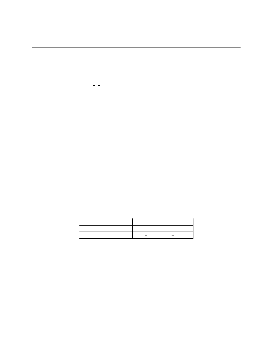
Chapter 3.2

Sometimes, one thinks about lockout/agreement and strike/agreement problems using a

game of chicken.

There are no dominant strategies for this game. There are two pure strategy equilibria,

and one, rather disastrous mixed strategy equilibrium. There is an interesting correlated
equilibrium in this game, (

) on ((Thru, Chicken), (Chicken, Thru)). This corresponds to

taking turns, and gives each an expected utility of 4 apiece. If these were boxing matches,
another testoserone poisoned activity, the ticket buyers would be shouting “Fix!!” In any
case, these games fit into the same category as the Stag Hunt and the Battle of the Partners.

Hawk-Dove games, the use of deadly force

One of the puzzles about competition between animals over resources is the rarity of the
use of deadly force — poisonous snakes wrestle for mates but rarely bite each other, wolves
typically end their fights with both alive and almost uninjured after the beaten wolf has
exposed their throat, male caribou struggle for mates by locking antlers and trying to push
each other around but rarely gouge each other. The puzzle is that the use of deadly force
against a rival who is not using it rather thoroughly removes that rival from the gene
pool, thereby giving an immediate selective advantage to the user of deadly force. The
problem with this argument is that it is only selectively advantageous to use deadly force
in a population full of non-users of deadly force.

Suppose that there is a prize at stake worth 50x (in utility terms) to each of two con-

testants, where x

∈ (0, 2). The contestants have two options, aggressive Display or deadly

Force. Display immediately runs away from Force. The utility of being seriously injured,
which happens

of the time if both use deadly Force, is

−100. Finally, the loss of time in

a long mutual display of aggression has a utility of

−10. With payoffs, the game, Γ(x), is

Display

Force

Display

(

−10, −10)

(0, 50x)

Force

(50x, 0)

(50(

− 1), 50(

− 1))

Strategically, this is the same as Chicken so long as x

∈ (0, 2).

The mixed strategy equilibrium is interesting from an evolutionary point of view — if we

thought of behavior as being genetically determined, then a population consisting of mostly
Display (resp. Force) users would give selective advantage to Force (resp. Display) users,
and this balancing pattern would be at work unless the population proportions matched the
mixed equilibrium probabilities.

Let α(x) be the probability that Display is used in the mixed equilibrium (or, in the

evolutionary story, the proportion of the population using Display). The formula is

α(x) =

− x

2.4

− x

, so that

dα(x)

−

0.4

(2.4

− x)

< 0.

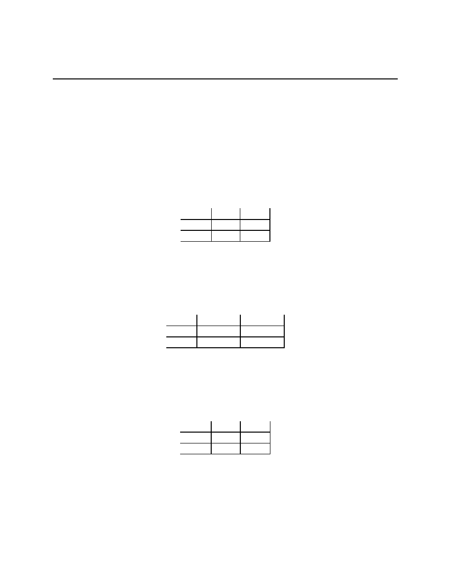
Chapter 3.2

The derivative being less than 0 means that the more valuable the prize is, the higher the
proportion of the time one would expect to see the use of deadly Force.

Note that α(2) = 0 so that Force is used all of the time. If x > 2, the formula for α(x)

breaks down (negative probabilities are no-no’s). For these values of x, Force is a dominant
strategy for both, and the game is, strategically, just like the Prisoners’ Dilemma game.

3.2.2

Rescaling and the strategic equivalence of games

Consider the 2

× 2 game

Left

Right

(a, e)

(b, f )

Down

(c, g)

(d, h)

where we’ve put 1’s payoffs in bold for emphasis. Since we’re assuming there are no ties

for player 1, a

6= c and b 6= d. Consider the function f

) given by f

(Left) =

−c and

(Right) =

−b. Lemma 1.4 tells us that adding f

to 1’s payoffs cannot change either CEq

or Eq. When we do this we get the game

Left

Right

− c, e)

(0, f )

Down

(0, g)

− b, h)

where we’ve now put 2’s payoffs in bold for emphasis. Since we’re assuming there are no
ties for player 2, e

6= f and g 6= h. Consider the function f

) given by f

(Up) =

−f and

(Down) =

−g. Lemma 1.4 tells us that adding f

to 2’s payoffs cannot change either CEq

or Eq. When we do this we get the game

Left

Right

(x, y)

(0, 0)

Down

(0, 0)

(r, s)

where x = a

− c, y = e − f, r = d − b, s = h − g, and x, y, r, s 6= 0. We’ve just proved that

all 2

× 2 games with no ties are equivalent to 2 × 2 games with (0, 0)’s in the off-diagonal

positions.

Applying this procedure to the six of the 2

× 2 games we’ve seen yields

Chapter 3.2

Prisoners’ Dilemma

Rational Pigs

Squeal

Silent

Squeal

(1, 1)

(0, 0)

Silent

(0, 0)

(

−1, −1)

Push

Wait

Push

(

−3.9, −1.1)

(0, 0)

Wait

(0, 0)

(1,

−2)

Matching Coins

Stag Hunt

(2,

−2)

(0, 0)

(2,

−2)

Stag

Rabbit

Stag

(9, 9)

(0, 0)

Rabbit

(0, 0)

(1, 1)

Battle of the Partners

Chicken

Dance

Picnic

Dance

(12, 8)

(0, 0)

Picnic

(0, 0)

(8, 12)

Chicken

Thru

Chicken

(

−10, −10)

(0, 0)

Thru

(0, 0)

(

−7, −7)

Once games are in this form, what matters for strategic analysis are the signs of the

utilities x, y, r, s, e.g. the sign patterns for the first two games are

Prisoners’ Dilemma

Rational Pigs

Squeal

Silent

Squeal

(+, +)

(0, 0)

Silent

(0, 0)

(

−, −)

Push

Wait

Push

(

−, −) (0, 0)

Wait

(0, 0)

(+,

−)

There are 2

possible sign patterns, but there are not 2

strategically distinct 2

×2 games.

We’re going to say that two games are strategically equivalent if they have the same sign
pattern after any finite sequence of (1) applying Lemma 1.4 to arrive at 0’s off the diagonal,
(2) relabeling a player’s actions, or (3) relabeling the players.

For example, in Rational Pigs, Little Pig was player 1 and Big Pig was player 2. If we

relabeled them as 2 and 1 respectively, we would not have changed the strategic situation at
all. We would have changed how we represent the game, but that should make no difference
to the pigs. This would give a game with the sign pattern

Push

Wait

Push

(

−, −) (0, 0)

Wait

(0, 0)

(

−, +)

If we were to relabel the actions of one player in Chicken, we’d have the game

(0, 0)

(

−10, −10)

(

−7, −7)

(0, 0)

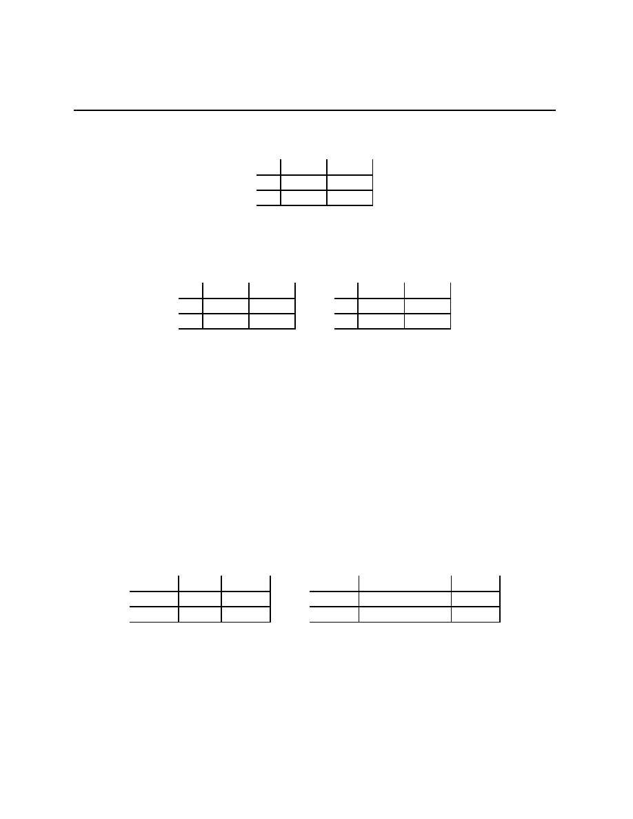
Chapter 3.3

which is equivalent, via Lemma 1.4, to a game with the sign pattern

(+, +)

(0, 0)

(+, +)

In just the same way, the following two sign patterns, from games like Matching Coins

are equivalent,

Matching Coins

Coins Matching

(+,

−) (0, 0)

(0, 0)

(+,

−)

(

−, +) (0, 0)

(0, 0)

(

−, +)

It is left as an exercise to show that all 2

× 2 games are equivalent to one of the four

categories identified at the beginning of this section.

3.3

The gap between equilibrium and Pareto rankings

The defining charateristic of an equilibrium is the mutual best response property. Pareto
optimality arguments are very peculiar from the mutual best response point of view.

3.3.1

Stag Hunt reconsidered

An implication of Lemma 1.4 is that the following two versions of the Stag Hunt are strate-
gically equivalent.

Stag Hunt

Hunting Stag

Stag

Rabbit

Stag

(S, S)

(0, R)

Rabbit

(R, 0)

(R, R)

Stag

Rabbit

Stag

− R, S − R)

(0, 0)

Rabbit

(0, 0)

(R, R)

Remember that S > R > 0, which makes the Pareto ranking of the pure strategy

equilibria in the first version of the game easy and clear. However, the Pareto rankings of
the two pure strategy equilibria agree across the two versions of the game only if S > 2R.
If R < S < 2R, then the Pareto criterion would pick differently between the equilibria in
the two strategically equivalent games.

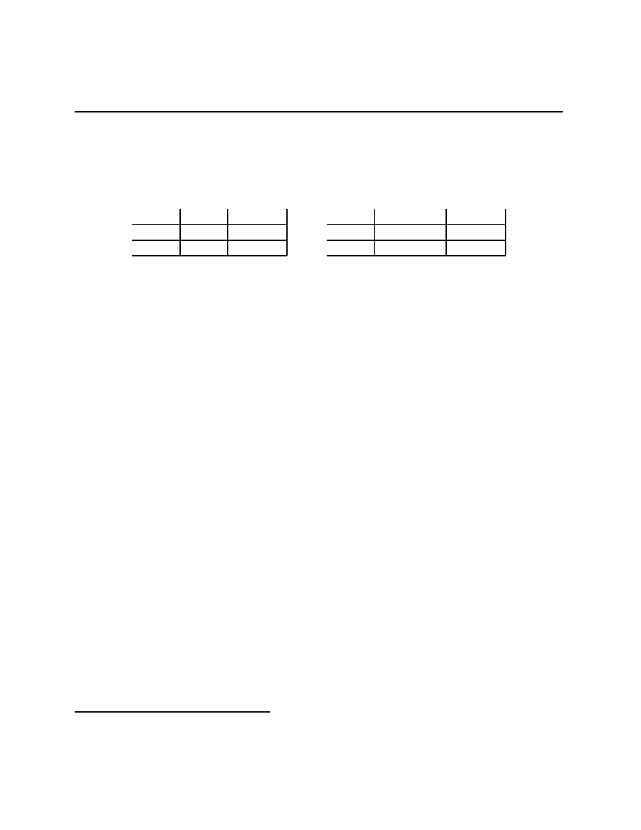
Chapter 3.3

3.3.2

Prisoners’ Dilemma reconsidered

An implication of Lemma 1.4 is that the following two versions of the Prisoners’ Dilemma
are strategically equivalent.

Prisoners’ Dilemma

Dilemma of the Prisoners

Squeal

Silent

Squeal

(1, 1)

(0, 0)

Silent

(0, 0)

(

−1, −1)

Squeal

Silent

Squeal

(

−14, −14) (0, −15)

Silent

(

−15, 0)

(

−1, −1)

If we take the Pareto criterion seriously, we feel very differently about the equilibria of

these two games. In the first one, the unique equilibrium is the Pareto optimal feasible
point, in the second, the unique equilibrium is (very) Pareto dominated.

3.3.3

Conclusions about Equilibrium and Pareto rankings

From these examples, we should conclude that the Pareto criterion and equilibrium have
little to do with each other. This does not mean that we should abandon the Pareto criterion
— the two versions of the Prisoners’ Dilemma are equivalent only if we allow player i’s choice
to add 15 years of freedom to player j

6= i. Such a change does not change the strategic

considerations, but it drastically changes the social situation being analyzed.

In other words: the difference between the two versions of the Prisoners’ Dilemma is

that we have stopped making one person’s action, Squeal, have so bad an effect on the
other person’s welfare. One might argue that we have made the game less interesting by
doing this. In particular, if you are interested in (say) understanding how people become
socialized to pick the cooperative action when non-cooperation is individually rational but
socially disastrous, the new version of the Prisoners’ Dilemma seems to be no help whatso-
ever. The new version has synchronized social welfare (in the Pareto sense) and individual
optimization.

My argument about socialization would be phrased in terms of changes to the utility

functions, though not necessarily the changes given in Lemma 1.4. Utility functions are
meant to represent preferences, and preferences are essentially indistinguishable from re-
vealed preferences, that is, from choice behavior. If one thinks that both being Silent is
the right outcome, then you need to change the preferences so that the players prefer being
Silent. Socialization is one very effective way to change preferences. Many people feel badly
if their actions harm others, even others they do not personally know. I take it that they
have preferences that include consequences to others. To study socialization to cooperative
actions, one needs to study how preferences are changed. Once again, much of the mileage
in game theory arises from the contrast between different games.

The NYT article covering blood flows in the brain.

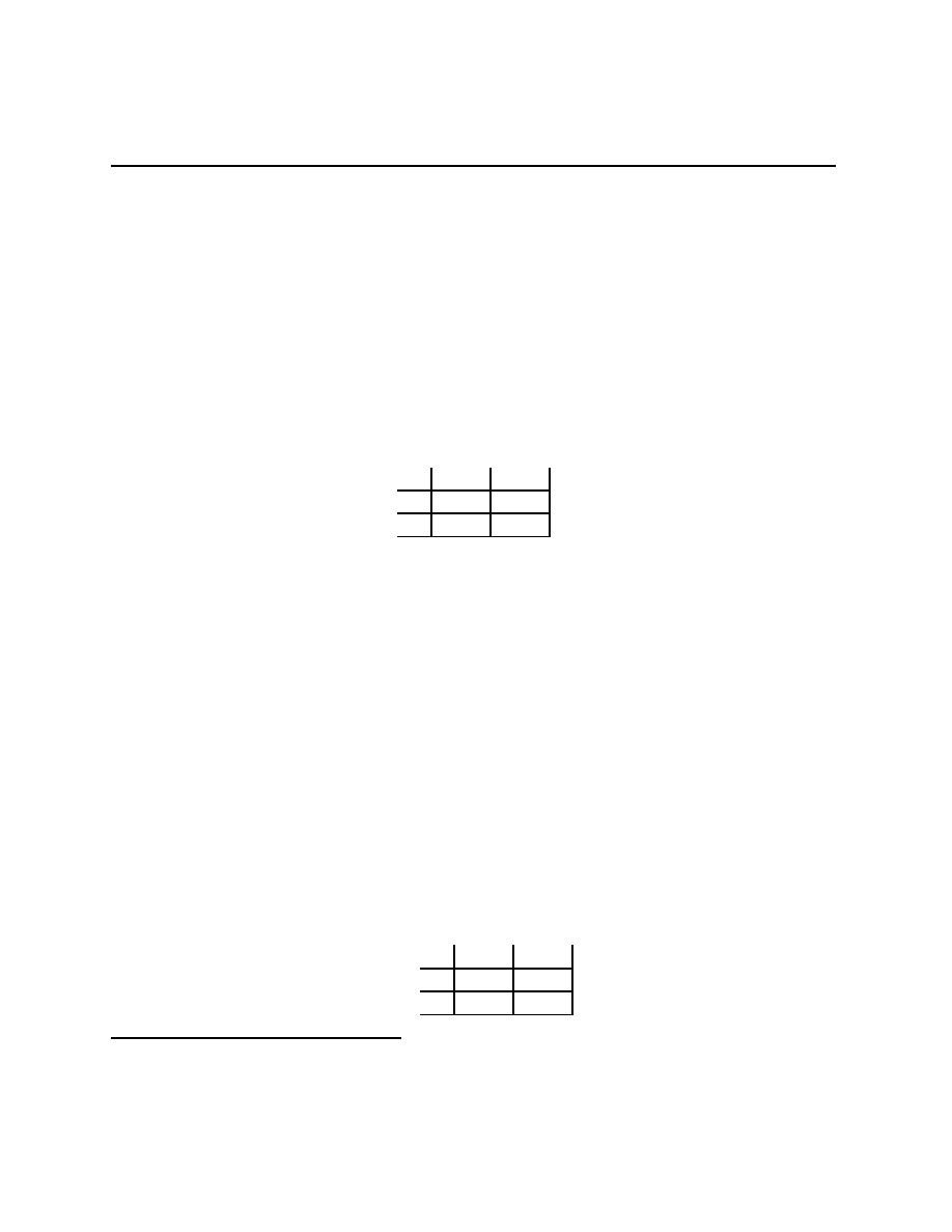
Chapter 3.3

3.3.4

Risk dominance and Pareto rankings

One possible reaction to the previous section is “Yeah, yeah, that’s all fine so far as the
mathematics of equilibrium is concerned, but when I write down a game with specified
payoffs, I really mean that those payoffs represent preferences, they are not merely devices
for specifying best responses.” If you take this point of view (or many points of view like it),
analyzing Pareto optimality again makes sense.

However, if you take this point of view, you

are stuck when you come to games in which the players disagree about which equilibrium
is better. One way to try to resolve this is using the idea of risk dominance.

In some coordination games, we (might have) favored one equilibrium outcome over

another because it was better for everyone. In the following game (with the same best
response pattern as the Stag Hunt), Pareto ranking does not work,

(5, 6)

(3, 2)

(0, 2)

(6, 4)

One idea that does work to pick a unique equilibrium for this game is called risk dom-

inance. The two pure strategy equilibria for this game are e

= (T, L) and e

= (B, R).

The set of σ

for which T , 1’s part of e

, is a best response for player 1 is S

{σ

(L)

≥ 3/8}. The set of σ

for which B, 1’s part of e

, is a best response for player 1 is

{σ

: σ

(L)

≤ 3/8}. Geometrically, S

is a larger set than S

. One way to interpret

this is to say that the set of beliefs that 1 might hold that make 1’s part of e

a best response

is larger that the set that make 1’s part of e

a best response. In this sense, it is “more likely”

that 1 plays his/her part of e

than his/her part of e

. Similarly, S

{σ

: σ

(T )

≥ 1/3}

is geometrically larger than the set S

{σ

: σ

(B)

≤ 1/3}, so that it is “more likely”

that 2 plays his/her part of e

than his/her part of e

. This serves as a definition of risk

dominance, e

risk dominates e

What we have just seen is that it is possible to invent a principle that takes over when

Pareto ranking does not pick between equilibria. There are at least two more problems to
overcome before we can reach an argument for systematically picking a single equilibrium,
even in the set of 2

× 2 games that we have been looking at.

1. The two players may disagree about which equilibrium risk dominates as in

(5, 6)

(3, 5)

(0, 2)

(6, 4)

The previous section is just a bad dream to be ignored while you get on with the serious business of

proving that all works out for the best in this best of all possible worlds.

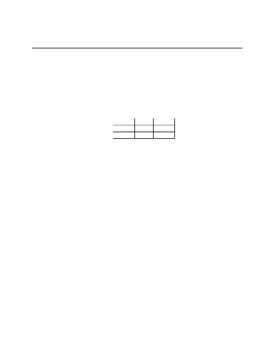
Chapter 3.4

which is the same as the previous game, except that 2’s payoff to (T, R) has been
changed from 2 to 5. The sets S

and S

are unchanged, but S

{σ

: σ

(T )

≥

2/3

} and S

{σ

: σ

(B)

≤ 2/3}. Now e

risk dominates e

for 1 but e

risk

dominates e

for 2.

2. Risk dominance may disagree with the Pareto ranking, so we actually need to decide

whether we believe more strongly in risk dominance than in Pareto ranking. Return
to the Stag Hunt,

Stag

Rabbit

Stag

(S, S)

(0, R)

Rabbit

(R, 0)

(R, R)

where S > R > 0. While (S, S)

(R, R)

, making S look good, for each hunter

the Rabbit strategy looks less ‘risky’ in the sense that they are less dependent on the
actions of the other. Arguing directly in terms of the risk dominance criterion, the Stag
equilibrium risk dominates if S > 2R, while Rabbit risk dominates of 2R > S > R.
However, Stag always Pareto dominates.

Even if Pareto rankings do not survive the utility transformations of Lemma 1.4, risk

dominance rankings do.

Problem 3.1 Suppose that a 2

× 2 game without ties, Γ = (A

, u

), has two pure strategy

equilibria, e

and e

and that e

risk dominates e

. Suppose that Γ

= (A

, v

) where the v

are derived from the u

using any of the transformations allowed in Lemma 1.4. We know

that e

and e

are equilibria of Γ

. Show that e

risk dominates e

in Γ

3.4

Other static games

These will be divided into finite games and infinite games.

3.4.1

Infinite games

Infinite games are those in which the space A =

i∈I

is infinite. This can happen if one

or more of the A

is infinite, or if I is infinite. Both are interesting, and sometimes both are

interesting simultaneously.

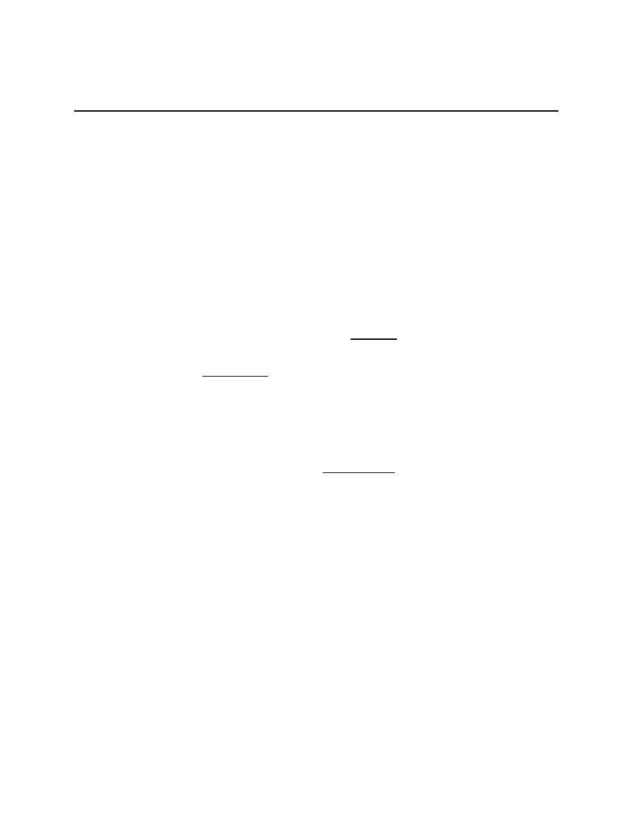
Chapter 3.4

Tragedy of the commons

There are I different countries that can put out fishing fleets to catch from pelagic schools
of fish. Use the number a

∈ R

= A

to represent the number of fishing boats in the fleet

of country i, i = 1, . . . , I. To finish specifying the game, the utilities, u

: S

→ R need to be

specified.

The marginal cost of a boat is constant, and equal to c. For given a

∈ A, let n = n(s) =

i∈I

and n

−i

(s) =

j6=i

. When the total number of boats is n, the per boat return

is v(n) where v(0) > 0, v

(n) < 0, v

(0) < c, and v

(n) < 0. For country i, the benefit

to putting out a fleet depends on the size of their own fleet, a

, and the size of the other

countries’ fleets, n

−i

(s),

, n

−i

(s)) = s

v(s

+ n

−i

(s))

− cs

= a

v(n(s))

− cs

For fixed n

−i

= n

−i

(s), u

(

·, n

−i

) is concave because

∂u

−i

)

∂s

= v(n) + a

(n)

− c, implying

∂

, n

−i

)

∂s

= v

(n) + a

(n) + v

(n) < 0.

Let us imagine that time is indexed by t

∈ {0, 1, . . .} and a

i,t

represents what player i is

doing at time t. One possible dynamic process by which each country might adjust toward
fleet sizes that are better for them is

i,t+1

= s

i,t

+ α

∂u

i,t

, n

−i,t

)

∂s

> 0, moves a

i,t+1

in the direction that increases u

, larger steps for larger α

and larger

∂u

i,t

, n

−i,t

)/∂s

. A variant of this kind of dynamic is

i,t+1

= α

i,t

+ (1

− α

∗

−i,t

)

where a

∗

−i,t

) is i’s best response to a fleet size of n

−i,t

by the other countries. This moves

i,t+1

of the way from a

i,t

toward the best response. Given the concavity of u

(

·, n

−i

), we

could, more generally, ask for a dynamic of the form

i,t+1

− s

i,t

= ψ

i,t

, n

−i,t

)

with the property that

sgn (ψ

i,t

, n

−i,t

)) = sgn (s

∗

−i,t

)

− a

i,t

For many variants of the above dynamics, the a

i,t

converge (i.e. settle down as t grows

Chapter 3.4

large), for many others, they do not converge. We can ask: If such a dynamic process
ψ = (ψ

)

i∈I

has an equilibrium, a

∗

= (s

∗

)

i∈I

, that is, a point at which a

∗

i,t+1

= s

∗

i,t

, what

does it look like? Well, note that a

∗

= 0 is not possible because the dynamics would push

all of the a

i,t+1

up, nor is an a

∗

with the property that v(n(s

∗

))

≥ c because the dynamics

would push all of the a

i,t+1

down. At an equilibrium of the dynamic process,

(

∀i ∈ I)[s

∗

i,t+1

− s

∗

i,t

= ψ

∗

i,t

, n

−i

∗

)) = 0]

so that

∗

i,t

= s

∗

−i,t

which, given the differentiability and concavity, is equivalent to

(

∀i ∈ I)

∂u

∗

, n

∗

−i

)

∂a

= 0

(3.1)

The simultaneous satisfaction of the best response conditions gives the Nash equilibrium.

In this game, the Nash equilibrium is inefficient compared to binding agreements to limit
fleet size, and the inefficiency grows with I. Strategic considerations do not lead to socially
optimal solutions.

Cournot competition

Two firms compete by producing quantities q

and q

of a homogeneous good, and receiving

profits of the form

, q

) = [p(q

+ q

)

− c]q

where p(

·) is the inverse market demand function for the good in question. Assume that

p(q) = 1

− q and that 0 ≤ c 1, work out the linear best response functions Br

), and

examine the dynamics

1,t+1

= Br

), t odd, q

2,t+1

= Br

), t even.

Note the global asymptotic stability.

Calculate the equilibrium q

∗

= q

∗

+ q

∗

and p

∗

= p(q

∗

). If we increase the number of

firms, I, lim

I→∞

∗

= c, a pleasing convergence to the competitive case.

Returning to cartels, suppose that firm 1 has a large capacity, but that the other firms,

the little pigs, have capacities q

, j

6= 1, much less than q

∗

/I. More formally, A

= [0, q

]

6= i, and A

= [0, q

] for some large q

Problem 3.2 Show that, in this case, the large firm acts as a monopolist for the residual
market, that is, for the market left over after the little pigs have produced q

Chapter 3.4

Bertrand competition

Two firms compete by setting prices p

, p

, consumers go to the lower price supplier (because

the goods are homogeneous), so that profits are

, p

) =






− c)q(p

)

if p

< p

[(p

− c)q(p

)] if p

= p

if p

> p

where q(

·) is the market demand function. If p

is less than or equal to the monopoly price

for the market, then there is no best response for i in [0, p

). However, the intuition is that

i undercuts j and vice versa. The only equilibrium of this kind of dynamic is p

= p

= c.

Here 2 firms are enough to arrive at the competitive outcome.

Note that both firms are better of with Cournot competition, and both firms prefer half

of the monopoly profits to the Cournot profits.

Cournot vs. Bertrand competition

Bertrand competition was invented as a criticism of Cournot competition. The argument
is that, since Cournot assumed the good to be homogenous, it must be that consumers will
only buy from the lowest price supplier, hence the above Bertrand dynamic. Comments:

1. In some industries, there is a long lag between production decisions and outputs (e.g.

acres planted now only deliver a harvest months in the future), and once the quantity
has been produced, it is individually better for each of the producers to sell all of their
output. This is closer to the Cournot story.

2. In other industries, quantity is quickly adjustable and price competition results. This

is closer to the Bertrand story.

3. Advertising textbooks stress the importance of not bringing price to the attention of

the consumer, that price competition is horrible and dangerous. They suggest trying to
distinguish the good from its competitors, a strategy not considered by either Cournot
or Bertrand.

4. In industries where differentiation is quite hard, say milk, the producers are likely to

form cartels to keep prices high and to coordinate advertising. Again, these consider-
ations are in neither the Cournot nor Bertrand models.

5. One might believe that installing production capacity is a difficult operation, and that

once it is installed, price competition emerges. Neither model is like this.

Chapter 3.4

6. For some goods, firms can carry inventories. This allows a huge variety of dynamic

strategies. Neither model is like this.

A larger point is that game models are ways of telling a variety of stories simultaneously

— by not naming the good being produced, the models cover a large area that is not
delineated except by the assumptions we bring to it. When is it that particular stories are
useful guides? Well, reaching a conclusion favoring powerful interests or being consonant
with widely held values means that the stories are more likely to be judged to be useful
guides. I am carefully distinguishing between being a useful guide and being judged to be
a useful guide.

Rather than analyze the political economy of intellectual work done in universities that

are growing more corporatized, the profession adopts a variety of strategies that are not
particularly convincing — refuge in a very conservative and well-refuted model of science as
hypothesis testing, not thinking about the issue at all, sometimes by calling it “exemplifying
theory.”

I want you to come out of this class able to reason using game theory models. I also

want you to come out thinking that economics is dominated by analyses that function to
support the status quo. One can use game theory in more interesting ways, and there are
examples below.

Fable of the Bees

In the Stag Hunt, there is a productive role for a coordinator of actions. This coordinator
can be a person, or it can be a tradition. In any case, what is required is a random signal.
When the signal is commonly observed, economists often call it a “sunspot.” Coordination
seems to be particularly important in macroeconomics. An extended version of coordination
reasoning is in the Fable of the Bees, originally from Bernard Mandeville, but we mostly
know it from John Maynard Keynes.

Here are two versions of the Fable. These contain almost everything I have retained from

courses about macroeconomics.

Both games will involve an infinite number of players, but

neither depends on this particular technical device for anything but convenience.

Fable of the Bees #1: Each person ω in the set of people Ω chooses an action a

∈ R

to solve

max

∈R

, a)

− c

where c

> 0, u

is monotonic in both arguments, a =

Ω

dµ(ω) for some (non-atomic)

probability µ on Ω. We assume that there is a unique solution a

∗

(a) exists and increases

This reflects badly on me, not on my teachers.

Chapter 3.4

with a, as it would if, for example,

∂

(

·, ·)

∂a

> 0.

We also assume that the mapping ω

7→ a

∗

is measurable (as it would be if the mapping

7→ u

is measurable and µ is a complete probability measure, and any probability measure

can be completed). Define

α(a) =

Ω

∗

(a) dµ(ω).

Any a such that α(a) = a is an equilibrium aggregate level of activity. Note that α(

·) is

increasing, in the differentiable case,

dα(a)

Ω

∂a

∗

∂a

dµ(ω) > 0.

This suggests that it is possible, and it is, to arrange matters so that there are many different
equilibrium a’s. At any equilibrium, each person is choosing their own (unique) strict best
response to the actions of others.

Problem 3.3 Suppose that a

and a

are both equilibrium aggregate levels of activity in Fa-

ble of the Bees #1. Show that if a

> a

, then everyone strictly prefers the a

equilibrium

to the a

equilibrium.

Fable of the Bees #2: With the same set of people as above, each person ω

∈ Ω picks

present demand, d

, and savings for future demand to maximize

, (1 + r)a

) subject to d

+ a

= m

, d

, s

≥ 0,

where

r = r(d), r

(d) > 0, d =

Ω

dµ(ω),

and the mapping ω

7→ u

(

·, ·) is measurable. In other words, the more people spend now,

the higher the level of economic activity, d, which leads to a higher return on capital, r(d),
which means more to spend next period for each unit saved. For any given d, denote by
(d

∗

, s

∗

) the solution to the problem

max u

, (1 + r(d))a

) subject to d

+ a

= m

, d

, s

≥ 0.

For many reasonable specifications of u

(

·, ·), d

∗

ω(

·) is increasing in d, for even more speci-

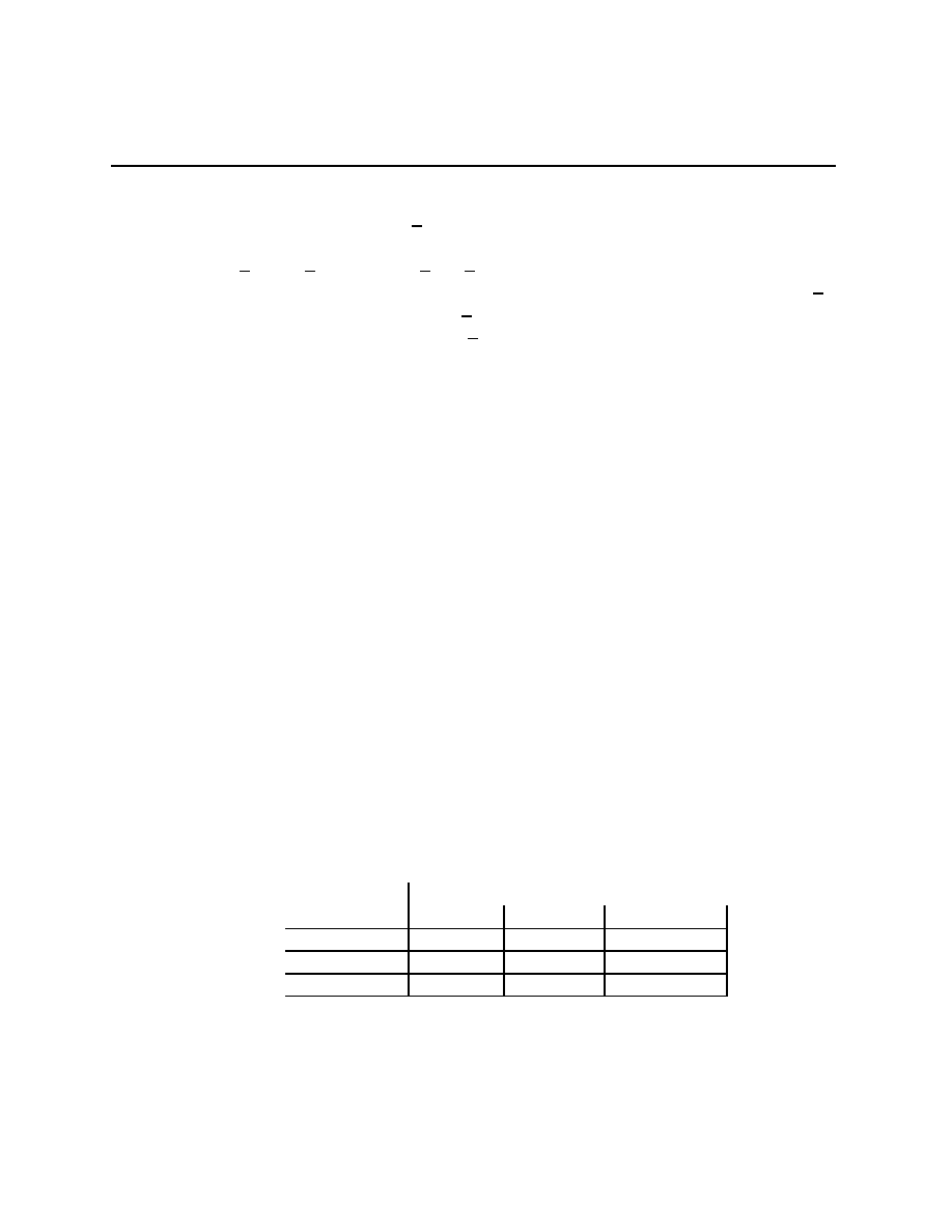
Chapter 3.4

fications,

δ(d) :=

Ω

∗

dµ(ω)

is increasing in d. Any d such that δ(d) = d is an equilibrium aggregate level of demand
activity, and it can be arranged that there are many equilibria. Equilibria with higher d’s
are strictly prefered to equilibria with lower d’s. An alternate version of this has r fixed but
has each m

being an increasing function of d, and, presuming the two consumption goods

are normal, the same basic story goes through.

These stories can be re-cast as stories about people not internalizing the external effects

that their own actions take.

3.4.2

Finite Games

Finite games are those in which the space A =

i∈I

is finite. This requires both I and

the A

to be finite (modulo a non-triviality assumption that #A

≥ 2).

Trust in electronic commerce

The E-Bay auction for a Doggie-shaped vase of a particularly vile shade of green has just
ended. Now the winner should send the seller the money and the seller should send the
winner the vile vase. If both act honorably, the utilities are (u

, u

) = (1, 1), if the buyer

acts honorably and the seller dishonorably, the utilities are (u

, u

) = (

−2, 2), if the reverse,

the utilities are (u

, u

) = (2,

−2), and if both act dishonorably, the utilities are (u

, u

) =

(

−1, −1).

For a (utility) cost s, 0 < s < 1, the buyer and the seller can mail their obligations to a

third party intermediary that will hold the payment until the vase arrives or hold the vase
until the payment arrives, mail them on to the correct parties if both arrive, and return the
vase or the money to the correct party if one side acts dishonorably. Thus, each person has
three choices, send to the intermediary, honorable, dishonorable. The payoff matrix for the
symmetric, 3

× 3 game just described is

Seller

Intermed.

Honorable

Dishonorable

Intermed.

1-s , 1-s

1-s , 1

-s , 0

Buyer

Honorable

1 , 1-s

1 , 1

-2 , 2

Dishonorable

0 , -s

2 , -2

-1 , -1

Problem 3.4 The first three questions are about finding the unique equilibrium, the last
two lead to interpretations.

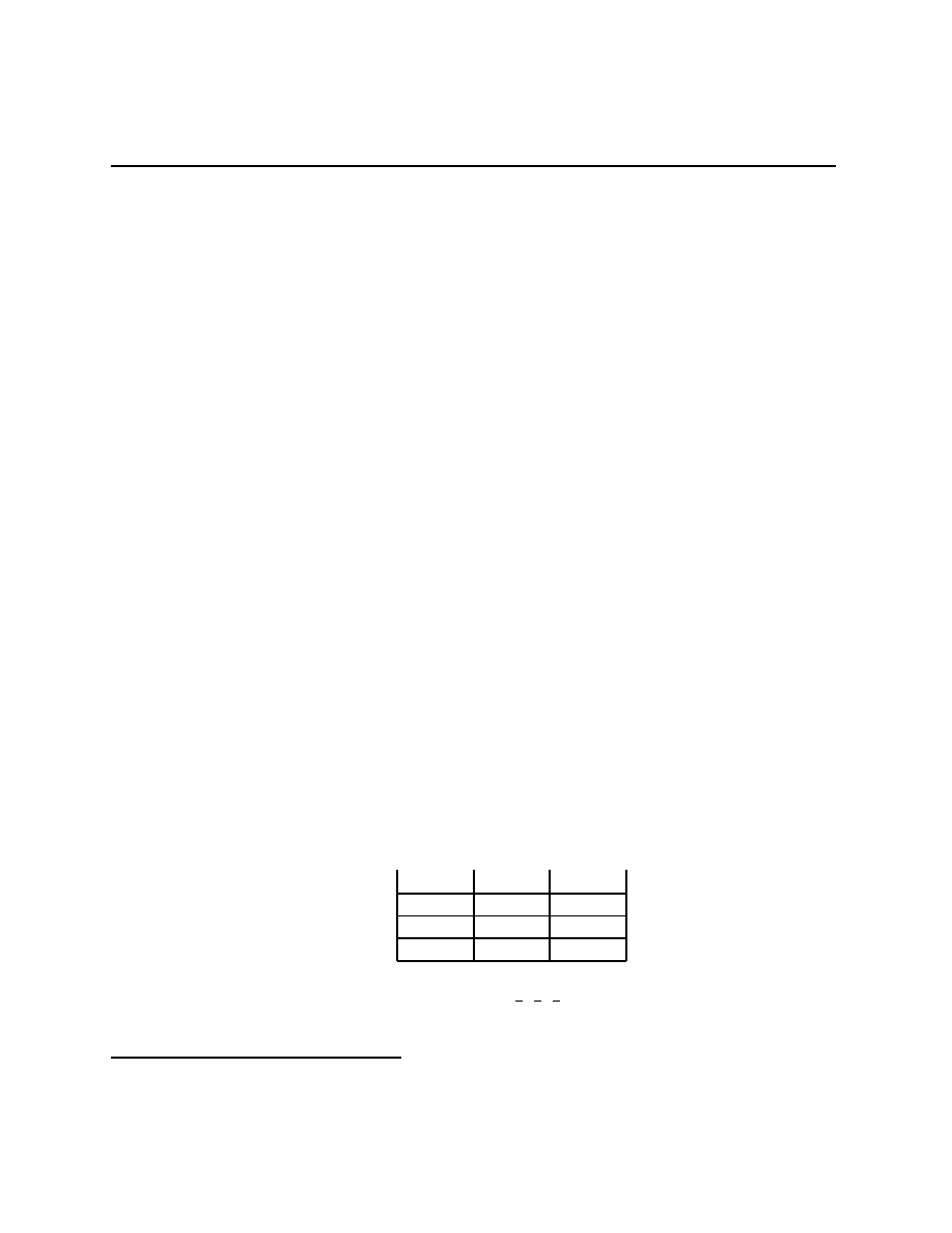
Chapter 3.4

1. Show that there is no pure strategy equilibrium for this game.

2. Show that there is no mixed strategy equilibrium involving the seller playing exactly

two strategies with strictly positive probability.

3. Find the unique mixed strategy equilibrium and its expected utility as a function of s.

4. For what values of s is the probability of dishonorable behavior lowest? Highest?

5. What is the equilibrium of this game without the existence of an intermediary? If the

intermediary is a monopolist, what will they charge for their services?

One of the really perverse aspects of this situation is that the availability of an intermedi-

ary is what makes trade possible, but people are willing to incur the cost of the intermediary
only because there continues to be cheating. This is much like the monitoring games.

It is the S.E.C. and honest accounting that has made the vigor of the U.S. stock market

historically possible. We expect to have a positive frequency of cheating. The current levels
of cheating seem higher than is consistent with continuing to receive the benefits of having
a smoothly functioning stock market.

The sex lives of lizards

The males of the lizard species Uta stansburiana come in three distinct types: orange-
throats, blue-throats, and yellow-striped.

The orange are violently aggressive, and keep

large (up to size 7) harems, and defend large territories. The blue are less aggressive, keep
small (usually 3) harems, and defend small territories. The yellows are very docile, and look
like females, so they can infiltrate another male’s territory and secretly copulate with the
females. The oranges have such large territories and harems that they cannot effectively
guard against the yellows, though they can outcompete the blues. The blues, having smaller
territories, can guard against the yellows, but lose to the oranges. With payoffs, one version
of this game is

Orange

Blue

Yellow

Orange

(0,0)

(+1,-1)

(-1,+1)

Blue

(-1,+1)

(0,0)

(+1,-1)

Yellow

(+1,-1)

(-1,+1)

(0,0)

There is only one equilibrium for this game, (

). It is a bit hard to think about

this as the equilibrium of a two player game though — the lizards are not choosing what

This is [3, Game 4.16, p. 67-8].

Chapter 3.6

color to be born. However, if we imagine that there is a population story at work, we might
get someplace. Loosely, suppose that there is a population of lizards in which the orange
predominate. This means that the yellow will thrive, soon outbreeding the testoserone
poisoned oranges. But once the yellows predominate, the blues will thrive, soon outbreeding
those sly yellows. But once the blues predominate, the oranges will thrive by beating up
those wimpy, second rate terretorialist blues. But once the orange predominate, . . . . We
might expect, over time, to average out to (

) as the population proportions.

3.5

Harsanyi’s interpretation of mixed strategies

It is perhaps not intuitive that people “flip coins,” that is, randomize, when making de-
cisions. When we think of correlated equilibria, this is not a problem — the randomness
can come from the signals. In some games, Matching Coins and the Inspection Games for
example, there is a strategic purpose to being unpredictable. These games also illustrate
that we need randomization for the existence of correlated equilibria. However, you do not
actually need to be unpredictable in some absolute sense so long as you are unpredictable
to the other player(s). This is what Harsanyi saw and proved.

Another intuitive way to understand mixed strategies is as follows: Everyone has little

idiosyncracies, my belief that you are randomizing can be recast as my belief that you are
not randomizing but that you yourself are random. More specifically, your choice depends
on your idiosyncracies, and so far as I am concerned, your idiosyncracies are random.

Fix a finite collection (A

)

i∈I

. We will parametrize games Γ(u) by u

∈ R

#S×#I

. Harsanyi’s

theorem is a statement about the mixed equilibria of “most” Γ(u). Define a set to be neg-
ligible in

#S×#I

if its closure has no interior.

Let (θ

)

s∈A,i∈I

be an independent collection of #S

× #I random variables on [−1, +1]

with smooth densities p

. For > 0, perturb the game Γ to ˜

(u) by setting the utilities to

= u

+ θ

. In the game ˜

(u), the players are told their own utilities, ˜

, but not the

utilities of the other players. Given their own utilities, the players choose their actions and
receive payoffs ˜

(a) if a occurs. A pure strategy equilibrium for ˜

(u) is an equilibrium in

which the set of ˜

that are playing mixed strategies has probability 0. For a pure strategy

equilibrium ˜

of ˜

(u), let D(˜

) denote the distribution over S induced by play ˜

. Let

Eq(˜

(u)) denote the set of pure strategy equilibria.

Theorem 3.6 (Harsanyi) Outside a negligible set of u, lim

→0

D(Eq(˜

(u))) = Eq(Γ(u)).

In other words, little idiosyncracies can be used to interpret mixed strategy equilibria.

Chapter 3.6

3.6

Problems on static games

There are problems are scattered through this chapter.

Problem 3.5 Show that all 2

×2 games with no ties have four strategic equivalence classes:

Games in which both players have a dominant strategy; Games in which exactly one player
has a dominant strategy; Games in which neither player has a dominant strategy and there
are three equilibria; Games in which neither player has a dominant strategy and there is
only a mixed strategy equilibrium.

Problem 3.6 Let n

∗

(I) denote the equilibrium size of the fishing fleet in the Tragedy of

the Commons model given above. Show that n

∗

(I) and the loss of efficiency increases in I.

[Hint: add the I FOC’s in (3.1) and compare to the FOC for the social optimum.]

Problem 3.7 Suppose that Γ is a finite game. Show that the following are equivalent:
(1) µ

∗

is an equilibrium for Γ,

(2) (

∀i ∈ I)(∀a

∈ A

)[u

(µ

∗

)

≥ u

(µ

∗

)], and

(3) (

∀i ∈ I)(∀a

∈ A

)[[µ

∗

) > 0]

⇒ [a

∈ Br

(µ

∗

) ]].

Further, show that if µ

∗

is an equilibrium for Γ and µ

∗

) > 0 and µ

∗

) > 0, then

(µ

∗

) = u

(µ

∗

Problem 3.8 [Optional ] Generalize the last problem to the case where each A

is a compact

metric space, each u

is jointly continuous on S, and each ∆

represents the set of countably

additive, Borel probabilities on A

Problem 3.9 Imagine that voters can be evenly spread out on an ideological spectrum from
left to right, say on the interval [

−M, +M], M > 0. There are two candidates who are trying

to get elected. The candidates announce positions someplace in the interval [

−M, +M], and

the voters vote for the candidate whose announced position is closest to their own.

1. Find the equilibrium positions announced by the two candidates.

2. Suppose that voters are happiest if they can vote for someone who closely represents

their point of view, whether or not that candidate wins. Specifically, suppose that
the happiness of the voter at position v

∈ [−M, +M] is 1 − |v − c| where c is the

position announced by the nearest candidate. What pair of announcements makes
voters happiest on average?

Problem 3.10 Radio stations choose the songs they play to attract the audience they are
trying to sell to advertisers. The larger the audience, the higher the profits. Suppose that they
divide songs along two dimensions, lyrics and energy. The lyrics range from thoughtful to

Chapter 3.6

stupid, and the energy level ranges from soothing to high voltage. The space of possible songs
can be thought of as the rectangle running along the interval [

−L, +L] for the intelligence of

the lyrics, and along the interval [

−E, +E] for level energy. Suppose that the most prefered

type of song for radio listeners are evenly spread over the two dimensional space of song
characteristics, and that they tune to that station with average songs closest to their most
prefered type.

1. Two radio stations are competing for audience share in the space of songs described

above. Find their equilibrium positions.

2. If there are three radio stations, show that there are no pure strategy equilibria.

3. (Hard!) Find or characterize the mixed strategy equilibrium for the case of three radio

stations.

Problem 3.11 One could object to there being only four equivalence classes of 2

× 2 games

with no ties — all of the coordination games are lumped together whether or not there is
unanimity in the rankings of the two pure strategy equilibria. Such an argument would say
that the Stag Hunt is a different kind of situation than the Battle of the Partners because
the hunters agree which is the better equilibrium, but the partners do not. Comment.

Chapter 4

Extensive Form Games: The Basics
and Dominance Arguments

Readings: These notes, Fudenberg & Tirole, Ch. 2 (especially about iterated dominance
arguments), & Ch. 3. Gibbons Ch. 2 & 4.

The class of extensive form games contains the static games we looked at in the previous

chapter. New to extensive form games are the informational and the dynamic issues. We’ll
begin by looking at a number of game trees, verbally describing the strategic situations they
are meant to represent, and, in some cases, finding the Nash equilibria. After having done
this often enough to see how useful a tool game trees are, the formal rules that game trees
must satisfy will (hopefully) look sensible.

A strategy for an extensive form game identified as a complete contingent plan for the

game tree. With this perspective, it is easy to go from game trees to static games. Going
back in the other direction involves seeing static games as extensive form games. This opens
a different, self-referentially justifying perspective on Nash equilibria. Iteratively applying
this notion does most of the work that we’ll do in shrinking the equilibrium set.

The next chapter will contain some of the mathematics we need to prove that equilibria

exist, that some kinds of iterative procedures for shrinking the set of equilibria will always
give a non-empty set of solutions, and that equilibrium sets depend, if not continuously on
the game, then at least upper-hemicontinuously.

4.1

Examples of extensive form game trees

The first observation is that static games have game tree representations, they are special
cases of extensive form games. After making this point and warning you that the formal
stuff is looming in your future, we’ll turn to a number of other classes of examples.

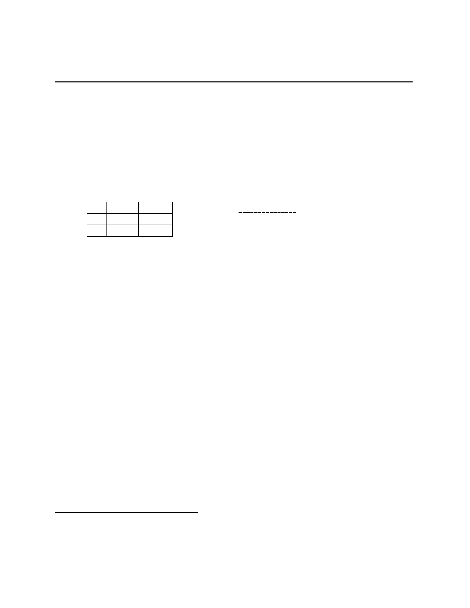
Chapter 4.1

4.1.1

Simultaneous move games as extensive form games

The point of simultaneous move games is that the players take actions in ignorance of
each others’ choices, not necessarily that the actions take place at exactly the same time.

Remember “Stag Hunt”? This 2

× 2 game has two representations, one of which we used

above:

(S, S)

(0, R)

(R, 0)

(R, R)

o 1

S
S

R
R

The representation we used above is called the normal form, the new one is called an

extensive form. This is the canonical extensive form of a normal form game. Verbally,
the way to think of this new representation of the game is that player 1 is making a decision
before player 2 will make a decision, but that 2 will be in ignorance of 1’s decision in making
her/his decision. This verbal description is represented as a tree with two branches (arrows)
from the origin. The origin is the node labelled

o . The label “1” next to the origin indicates

that player 1 gets to choose at that first node. The choice of S

leads to node x, the choice

of R

leads to node y. The nodes x and y are also choice nodes. The dotted line, labelled

2, connecting x and y indicates that player 2 cannot distinguish between x and y. The set of
nodes,

{x, y} is an information set, and at this information set, player 2 has two choices.

One requirement is that the choices cannot depend on whether x or y has been reached.
This is because 2, the person making the decision, does not know which has been reached.
The choices for 2 are labelled S

and R

, leading to terminal nodes r and s if taken at x,

and leading to terminal nodes t and u if taken at y. The utilities are listed at the terminal
nodes, with 1’s utility being above 2’s (numbers increase, by convention, we count from top
to bottom and from left to right).

It should be pretty clear that we can do the above to any of the finite simultaneous move

games we saw above. It should also be clear that we can reverse the order of the players,
having 2 move first and 1 choose not knowing 2’s choice has the same effect.

There surely exist people who will argue with you about the physics of whether simultaneity is “truly”

possible. Personally, I really don’t care.

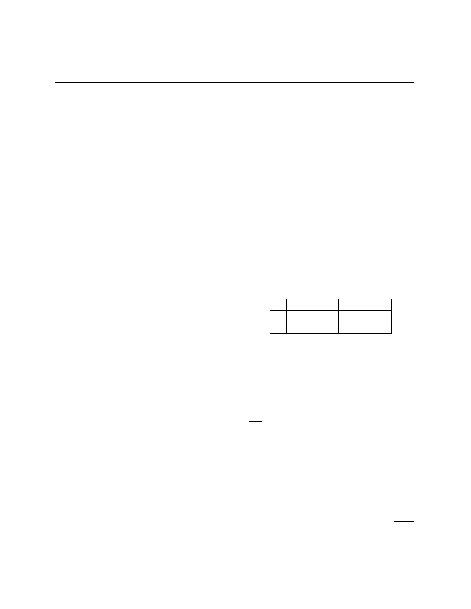
Chapter 4.1

4.1.2

Some games with “incredible” threats

In both of these games, there are Nash equilibria which involve one player believing that
another player is planning to use a strategy, which, were they actually called on to use, they
would avoid. That may sound garbled, let’s go to the games.

Atomic handgrenades

This is sometimes called the Chain Store paradox. You are approached by a fellow

carrying a certified atomic handgrenade. He says, “Give me 20$ or else I will explode this
small thermo-nuclear device.” Your choice is whether or not to give him the 20$. One
(not the only) representation of this situation has your two strategies being “Give 20$” and
“Don’t Give 20$”. The fellow’s strategies are “Blow up hand-held thermo-nuclear device
if not given 20$” and “Don’t blow up hand-held thermo-nuclear device if not given 20$”.
These are strategies that have conditional clauses in them. The extensive form and normal
form representations of the game are (where

−y −20):

−20

−y

Atomic Handgrenades

(

−20, −20) (−20, −20)

(

−y, −y)

(0, 0)

There are a couple of points to note. The nodes are not labelled (been there, done

that), there are two decision nodes and three terminal nodes, and the origin is still specially
marked. More importantly, the normal form is not one we’ve seen before because it has
ties,

−20 = −20, so that 2 is indifferent between l and r if 1 plays L. Find the set of

Nash equilibria as a function of y, of particular interest are the ones where 1 plays L with
probability 1. In the extensive form, the indifference corresponds to 2 not caring about
his/her action because L makes his/her choice moot. The equilibria involve 1 believing that
2 will do something (blow the two of them up), that he’d not do if his choice really mattered.
These are the 0 probability events discussed in the theory of choice under uncertainty, but
now the 0 probability is due to someone else’s strategic decision.

Compare the equilibrium sets when we do and when do not insist that people pick an

action that is optimal for some beliefs at 0 probability events. If we insist, then 2 must
play, or plan to play, r when they receive the signal that they should choose. This means

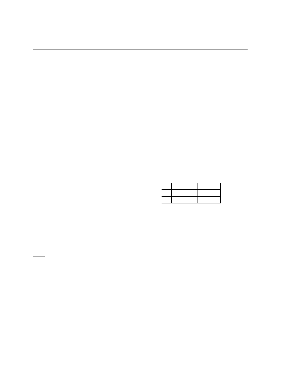
Chapter 4.1

that 1’s best reply is R. If we do not insist, then 1 can play L in equilibrium. 1 playing
L corresponds to 1 believing 2’s threat, so we are insisting that 1 not believe in any threat
that 2 would be unwilling to carry out.

A Puccini opera

In Puccini’s Gianni Schicchi, Buoso Donati has died and left his large estate to a

monastery. Before the will is read by anyone else, the relatives call in a noted mimic,
Gianni Schicchi, to play Buoso on his deathbed, re-write the will, and then convincingly
die. The relatives explain, very carefully, to Gianni Schicchi, just how severe are the penal-
ties for tampering with a will (at the time, they included having one’s hand cut off). The
plan is put into effect, but, on the deathbed, Gianni Schicchi, as Buoso Donati, rewrites
the will leaving the entire estate to the noted mimic and great artist, Gianni Schicchi. The
relatives can expose him, and thereby themselves too, or they can remain silent. With
player 1 being Gianni Schicchi and player 2 being the relatives, and some utility numbers
with y

200 to make the point, with Gianni Shicchi being player 1, we have

200

−y

200

Gianni Shicchi

(2, 200)

(

−y, −y) (200, 0)

Again, compare the equilibrium sets when we do and when do not insist that people

pick an action that is optimal for some beliefs at 0 probability events. If we insist, then 2
must play, or plan to play, r when they receive the signal that they should choose. This
means that 1’s best reply is R. If we do not insist, then 1 can play L in equilibrium. Again,
1 playing L corresponds to 1 believing 2’s threat, so we are insisting that 1 not believe in
any threat that 2 would be unwilling to carry out.

4.1.3

Handling probability 0 events

The previous games showed that thinking about behavior after 0 probability events shrinks
the set of Nash equilibria. We’re going to go back to the single person theory of choice under
uncertainty and introduce two ways of handling the 0 probability signals. They turn out

Chapter 4.1

to be the same for one person games, and in many, but not all, games with more than one
person. The terms we’ll use are perfect Bayesian equilibria and sequential equilibria.

Keep clear the following: we’re talking about putting limits on behavior that we’re

going to call “equilibrium behavior,” we’re asking for more than regular old expected utility
maximization.

We’ve got P

∈ ∆(S × Ω), β

:=marg

Ω

P (

·|π

−1

(s)), and the decision maker solves

max

a∈A

u(a, ω)β

(ω)

if marg

(P )(s) > 0. We let a

∗

(s) denote the solutions to that maximization problem. If

marg

(P )(s

◦

) = 0, then ex ante expected utility is unaffected by choices after s

◦

. Let S

◦

denote the set of s

◦

having probability 0 under P .

The perfect Bayesian approach asks that a

∗

P B

(s) be the solution set for

max

a∈A

u(a, ω)β

(ω)

when s

6∈ S

◦

, and a

∗

P B

◦

) be the solution set for

max

a∈A

u(a, ω)β

P er

(ω)

for some β

P er

◦

∈ ∆(Ω) when s

◦

∈ S

◦

The sequential approach asks that a

∗

seq

◦

) be the solution set for

max

a∈A

u(a, ω)β

◦

(ω)

for a consistent system of beliefs. Consistency asks that the beliefs at every s come from
some strictly positive approximation to, or perturbation of, P .

For P

0 a probability on S × Ω, let β

be the beliefs at s that come from Bayes’

Law, β

:= marg

Ω

(

·|π

−1

(s)). A system of beliefs s

7→ β

is consistent with P at s if

there exists a sequence P

0 such that P

→ P and β

→ β

. It is consistent with

P if it is consistent at all s. [Remember that “P

→ P ” means “∀ > 0 (no matter how

tiny),

∃N (probably very large), ∀n ≥ N, kP

− P k < .” The same definition applies to

→ β

Lemma 4.1 For any system of beliefs, s

7→ β

, that is consistent with P , β

= β

for all

6∈ S

◦

That is the first part of the observation that for single person decision theory, it turns

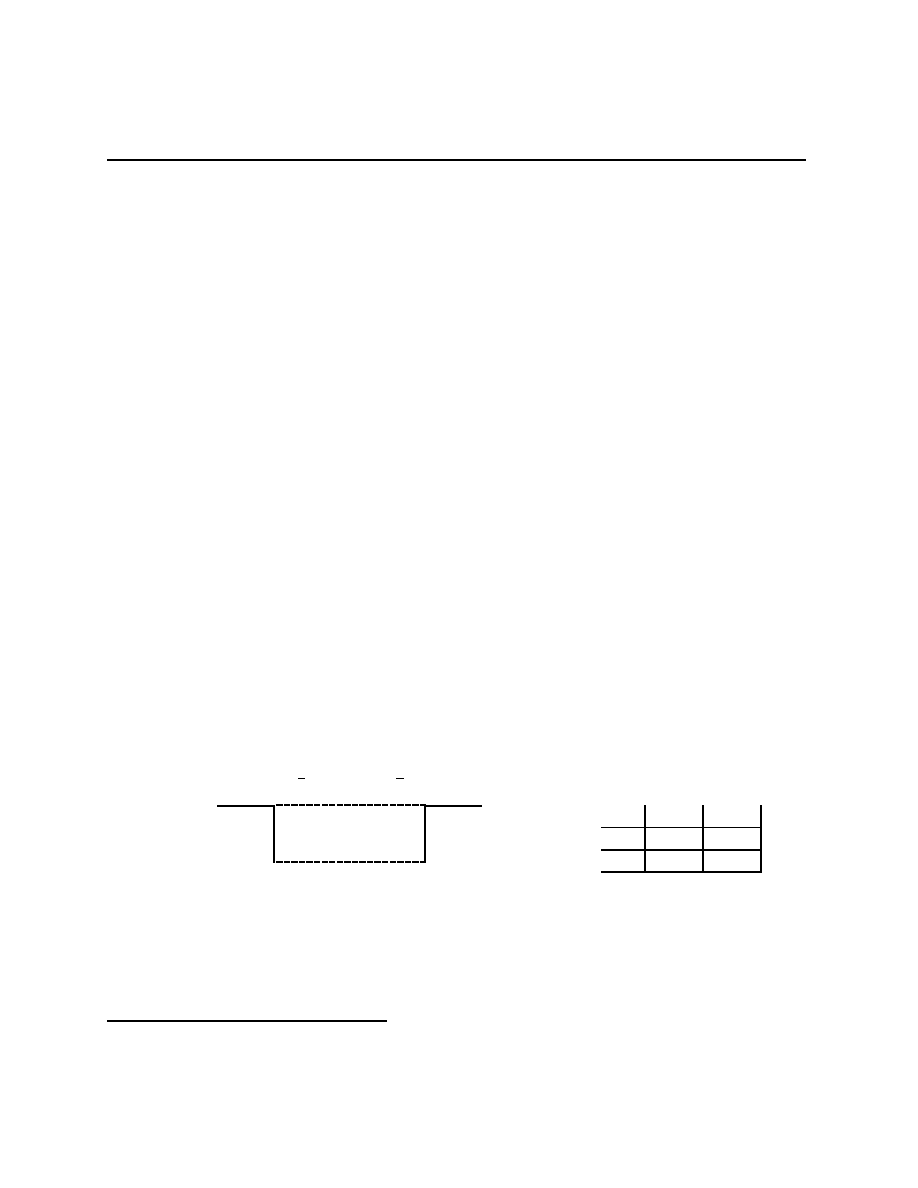
Chapter 4.1

out not to make any difference whether we pick beliefs out of a hat, as in the perfect
Bayesian approach, or ask that the beliefs arise from a perturbation of P , as in the sequential
approach. The second part is

Lemma 4.2 Any mapping from S

◦

to ∆(Ω) is consistent with P at every s

∈ S

◦

Applying either the perfect Bayesian criterion or the sequential criterion to the previous

two games, Atomic Handgrenades and Gianni Shicchi, gives the same answer, the threats
(to either explode the two players or to do something that causes both to have a hand cut
off) are not believed.

Important: When we apply the sequential criterion to games, we perturb the P for the

players’ optimization problem

1. in the same fashion for each person (this is consistent with the common prior assump-

tion), and

2. by individually perturbing each player’s strategy to be strictly positive, and then

maintaining the assumption of stochastic independence.

In some games, there is a distinction between the two criteria. As a rule, we tend to

opt for the the criterion that gives the smallest set of equilibria.

Since picking arbitrary

beliefs is less restrictive than using consistent beliefs, this means that sequential equilibria
are always pbe’s, but that the reverse is not necessarily true.

In the following game, there

are perfect Bayesian equilibria that have 1 playing out, and other perfect Bayesian equilibria
that have 1 playing in. Only the in equilibria are sequential. The reason that this is true is
that when we approximate the P , we insist that the players’ perturbations are stochastically
independent, that is, when we perturb P to P

, we do it by perturbing each player’s mixed

strategy, and then we then used the Nash independence of randomization.

out

(4, 1)

(6, 2)

out

(5, x)

This indicates that we’re not proud.

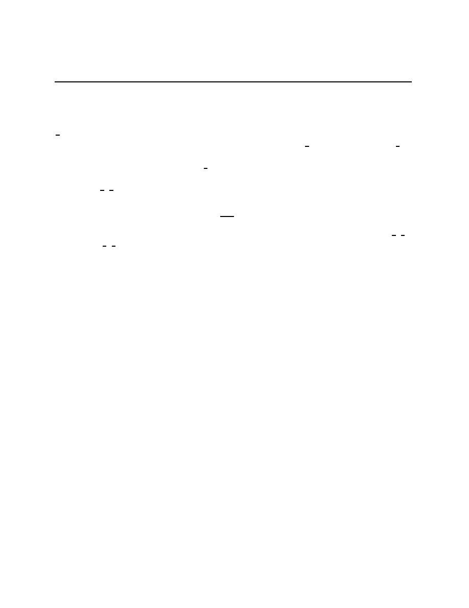
Chapter 4.1

The node,

, starts the game. It is where Nature, or some other version of randomness,

moves. Nature is sometimes called player 0, and has no strategic interests, that is, no utility
function, and no assumption of optimization. In this game, it plays L or R with probability

each. For the pbe’s involving 1 playing out, note that if 1 plays out, then 2’s signal to

play is a probability 0 event, and if we pick beliefs that assign

to the left node and

the right node in 2’s information set, then 2 is indifferent. So long as 2 is playing l with
probability greater than or equal to

, 1 is optimizing when playing out. When 1 plays

in, 2’s signal to play is a positive probability event, and Bayes’ Law applies, so 2’s beliefs
should be (

), in which case r is the strict best response. This in turn makes in a strict

best response for 1.

Now, to see that the out equilibria are not sequential, suppose that 1’s strategy of (1, 0)

on (out, in) is perturbed to something strictly positive, say σ

= (1

−

). Combining this

strategy with Nature’s stochastically independent randomization, β

for player 2 is (

and β

→ (

). Sequential equilibria require that 2 best respond to beliefs of this form,

and the unique best response is r. But that makes in, rather than out, a best response for
player 1.

4.1.4

Signaling games

These are an important class of games, and there are several examples here. Signaling
games have the following common features: there are 2 players, the one who moves first,
called the sender, knows something that the second, called the receiver, does not. Call that
something private information. The receiver can observe what the first one does, which
makes the action into a signal of sorts, but the receiver can not see the private information.
The private information and the actions taken by both players typically affect the utilities
of both. As we’ll see, in these games there is no distinction between pbe’s and sequential
equilibria, and neither shrink the set of equilibria unless the receiver has a weakly dominated
action.

A tale of poisoning

Felicia Casimirio worked for Acme. Acme had contracted with the defense department

to clean parts for high tech weapons. Cleaning the parts involved soaking them in a number
of solvents. The particularly dirty pieces also needed scrubbing. These were given to Felicia
who was ambitious for a promotion. Also, she never complained of the headaches, skin and
hair discoloration, dizziness, lethargy, or breathing problems that accompanied working
closely with these solvents in under-ventilated areas. Felicia contracted a rare and usually
lethal form of cancer. Acme claimed that it was a pre-existing condition, and would not pay
her medical expenses. Acme then fired her because she would no longer show up for work
on a regular basis. Fortunately, Felicia’s heretofore estranged older sister, Caridad, was a
lawyer, and Felicia asked for her help in suing Acme.

Chapter 4.1

Caridad explained to Felicia that in Acme’s experience, there was a 60% chance that

Felicia’s case, if taken to trial, would result in Acme paying high damages, 1000, and a 40%
chance that the trial would result in Acme paying low damages, 10 (units are $100, 000).
Because the break-in attempt at Felicia’s doctor had failed, the sisters were sure that, while
they knew whether or not Felicia’s case was a high damage case, Acme did not. Caridad
explained that Felicia could choose to offer to settle out of court for either 1000 or 10.
Acme would then either accept the offer and pay, or reject it and go to trial, a rather long
process. If Felicia’s was the high damages kind of case, by the end of the trial she would
be nearly dead, and this would prompt the jury to award double damages, 2000. If it was
the low damages kind of case, Acme’s private detectives would drag her name in the dirt
so badly that the award would be only

of the actual damages. Because of the effects on

their aging mother and having a (much) higher discount factor if she was indeed one of the
high damages cases, Felicia’s expected utility preferences can be represented by the numbers
given in in the game tree given below.

high

low

0.6

0.4

Felicia

Acme

−1000

−10

−2000

−1000

−10

−5

The node,

◦

, starts the game. It is where Nature, or some other version of randomness,

moves. Nature is sometimes called player 0, and has no strategic interests, that is, no utility
function, and no assumption of optimization. If Nature “chooses” high (low), Felicia has
the high (low) damages kind of cancer. This is the private information that Felicia has and
that player 2, Acme in this case, does not have. Another way to phrase this is that Felicia
receives a signal, h or l, and the signal affects her utility.

Chapter 4.1

One could regard Felicia as being different people in the two different cases, Felicia

and Felicia

. By the bridge crossing lemma, if she optimally decides at each node, she

maximizes her ex ante expected utility. Knowing her type of cancer, she has to decide on a
court strategy, asking for D

or asking for D

Acme sees her court strategy, but not her type of cancer, hence the pair of dotted lines,

one joining the nodes that follow the D

decisions, one joining the nodes that follow the D

decisions. In terms of signals, Acme sees either D

or D

, and here the distribution over

signals is a compound of Nature’s and Felicia’s choice, one non-strategic and one strategic.

After seeing the strategy/signal D

, Acme chooses between a

and r

, accepting and

rejecting the H settlement offer. After seeing the strategy/signal D

, Acme chooses between

and r

, accepting and rejecting the L settlement offer. Acme could also be regarded as

being a different economic actor in the two cases, one after seeing D

, and a different one

after seeing D

. These last choices lead to the terminal nodes, and the utility of player 1,

that is, Felicia, is given as the top of the two numbers.

There are a couple versions of the normal form for this game, depending on whether

you treat the players as being different. If you maximally differentiate, going with the
notion that people are the sum of their experiences and different experiences make you into
different people, you have four players, Felicia

, Felicia

, Acme

, and Acme

. This four

person game is called the agent normal form of the game. By bridge crossing, if the
agents maximize after forming signal-based beliefs using Bayes’ Law, they are maximizing
their ex ante expected utility.

The (standard) two person normal form for this game treats Felicia as the same person

thinking about her complete contingent plan. In this case, she has 4 (four, IV, that’s FOUR)
strategies, (D

, D

), (D

, D

), (D

, D

), and (D

, D

) where the ordered pair (a

, a

) is

the strategy of playing a

after seeing the signal h and playing a

after seeing the signal l.

To be really explicit here,

{(D

, D

), (D

, D

), (D

, D

), (D

, D

)

By this same logic, Acme has four strategies, (a

, a

), (a

, r

), (r

, a

), and (r

, r

{(a

, a

), (a

, r

), (r

, a

), (r

, r

)

Each choice of a

∈ A = A

× A

gives rise to an outcome, that is, to a distribution over

terminal nodes.

All that is left is to give the expected utilities associated with the different

outcomes.

We previously used the word “outcome” as the distribution over

A, the present usage as the distribution

over terminal nodes is consistent with the previous usage if we think about the canonical extensive form of
a normal form game.

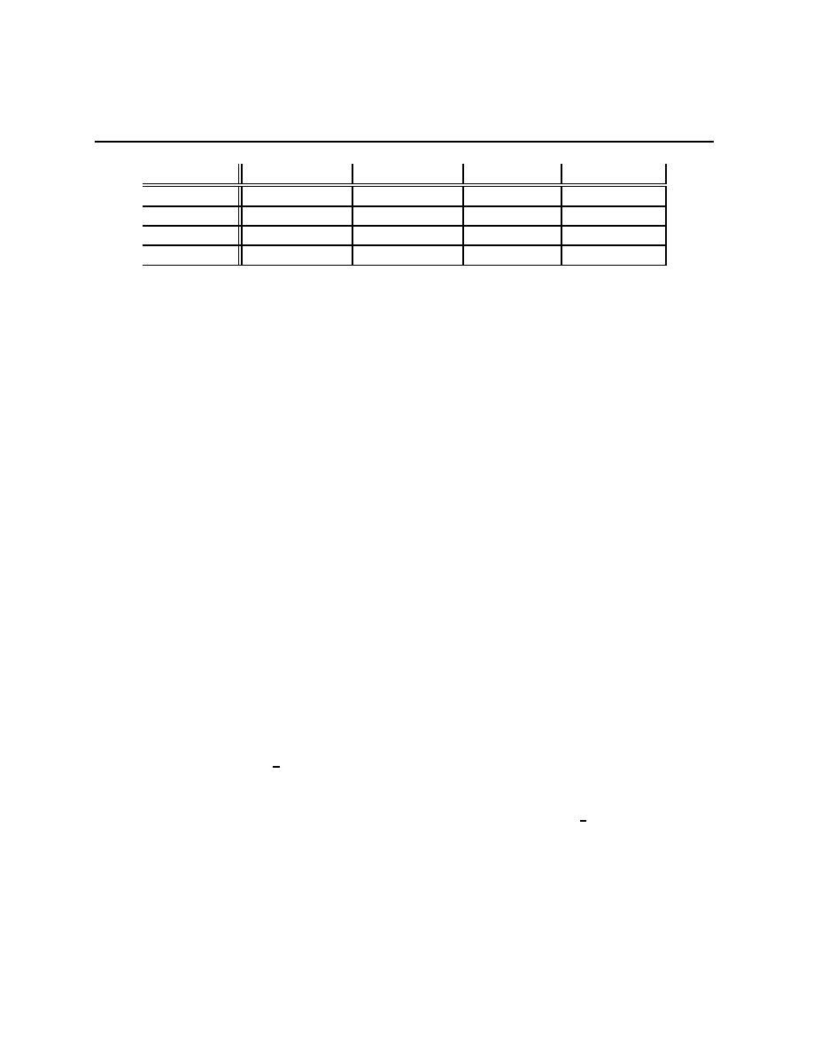
Chapter 4.1

↓ /A

→

, a

)

, r

)

, a

)

, r

)

, D

)

(5.0

−1000

)

(5.0

−1000

)

(2.4,

−1202) (2.4

−1202)

, D

)

(4.6,

−604)

(3.8,

−602

)

(2.8,

−1204) (2.0, −1202)

, D

)

(3.8,

−406)

(2.0,

−1600)

(3.0,

−8

)

(1.2,

−1202)

, D

)

(3.4,

−10

)

(0.8,

−1202)

(3.4

−10

)

(0.8,

−1202)

I’ve put stars, that is,

’s, next to the pure strategy best responses to pure strategies.

Thus, (D

, D

) is Felicia’s pure strategy best respone to both (a

, a

) and (a

, r

), while

either (a

, a

) or (a

, r

) are best responses for Acme to Felicia’s pure strategy of (D

, D

The mixed strategy β(a

, a

) + (1

− β)(a

, r

) corresponds to always accepting high set-

tlement offers while accepting β of the low settlement offers. These are all best responses
since they differ only on a signal having probability 0 given what Felicia is playing. These
are all Nash equilibria, the whole infinite set

{((D

, D

), β(a

, a

) + (1

− β)(a

, r

)) : β

∈ [0, 1]}.

This normal form game has ties, and it is not the case that there are an odd number of
equilibria.

The other pure strategy box with two

’s in it is ((D

, D

), (r

, a

)). Note that Acme has

two pure strategy best responses to Felicia playing (D

, D

), the one we’ve noted, (r

, a

and the strategy (a

, a

). The mixture β(a

, a

) + (1

−β)(r

, a

) corresponds to accepting

all low settlement offers and accepting β of the high settlement offers. These are all best
response for Acme to Felicia’s play of (D

, D

), but for some values of β, (D

, D

) is not a

best response for Felicia. Specifically, for (D

, D

) to be a best response, the inequalities

3.4

≥ 5.0β + 2.4(1 − β), 3.4 ≥ 4.6β + 2.8(1 − β), and 3.4 ≥ 3.8β + 3.0(1 − β)

must be satisfied. Doing the algebra, these are the inequalities

≤ 5/13, β ≤ 1/3 and β ≤ 1/2,

so that only the β

∈ [0,

] satisfy all the inequalities. This gives a second set of Nash

equilibria, the set

{((D

, D

), β(a

, a

) + (1

− β)(r

, a

)) : β

∈ [0,

]

Bridge crossing delivers this set of equilibria in a simpler fashion. Felicia’s signals happen

with positive probability. For (D

, D

) to be a best response,, D

must be optimal after

both signals. For Felicia

, that is, for Felicia after she sees the high signal, this depends on

whether or not her payoff to D

is greater than her payoff to D

, 3

≥ 5β + 2(1 − β), that

Chapter 4.1

is, β

≤

. For Felicia

, this is the inequality 4

≥ 5β + 3(1 − β), that is, β ≤

. Only the

∈ [0,

] satisfy both inequalities.

Okay, that worked, but why did we have only two inequalities rather than the three we

had before? The answer comes out of the bridge crossing lemma, the inequality that was
not reproduced involved changing what Felicia was doing from (D

, D

) to (D

, D

), that

is, changing her action after both signals. Bridge crossing says that it’s enough to check
one signal at a time, and what we saw was that checking the double change gave rise to
a redundant inequality. To be really really really specific here, changing from (D

, D

) to

, D

) gave rise to the inequality β

≤

, and since

, this means that β

≤

makes

the inequality β

≤

redundant.

Will that be beer, or quiche for breakfast?

This game is due to Cho and Kreps (1987), who tell a version of the following story:

There is a fellow who, on 9 out of every 10 days on average, rolls out of bed like Popeye on
spinach. When he does this we call him “strong.” When strong, this fellow likes nothing
better than Beer for breakfast. On the other days he rolls out of bed like a graduate student
recovering from a comprehensive exam. When he does this we call him “weak.” When weak,
this fellow likes nothing better than Quiche for breakfast. In the town where this schizoid
personality lives, there is also a swaggering bully. Swaggering bullies are cowards who, as a
result of deep childhood traumas, need to impress their peers by picking on others. Being
a coward, he would rather pick on someone weak. He makes his decision about whether to
pick, p, or not, n, after having observed what the schizoid had for breakfast. With payoffs,
the game tree is

strong

weak

0.9

0.1

beer

quiche

Bully

−10

Chapter 4.1

This is not only a psycho-drama, it’s also a story about entry-deterrence. To get to that

story, re-interpret the schizoid as an incumbent who may or may not have found a cost-
saving technology change. If they have, it makes them a stronger competitor. This private
information is not known to player 2, the potential entrant. The incumbent can start an
aggressive advertising campaign, something they’d like better if they were strong, that is,
if they have found the cost-saving change to their technology. The potential entrant would
rather compete against a weak incumbent than a strong incumbent, but can condition their
entry decision only on whether or not they see the aggressive advertising campaign.

Problem 4.1 Give the 4

× 4 normal form for this game and find the two set of equilibria.

Two other variants of entry-deterrence

Consider a market with one incumbent firm and a potential entrant. The potential

entrant has low costs with probability 0.2, and has high costs with probability 0.8. The
actual costs (low or high) of the entrant are private information to the entrant, who decides
whether to stay “out” or “enter.” The outside option for the low cost entrant has an expected
utility of 25, while the outside option for the high cost entrant has an expected utility of
0. If the potential entrant stays out, then the incumbent has an expected utility of 25. If
the potential entrant enters, then the incumbent decides whether to “fight” or “acquiesce.”
If the incumbent fights, then the payoffs for the entrant and incumbent respectively are
(20,

−25) when the entrant is low cost, and (−10, 40) when the entrant is high cost. If the

incumbent acquiesces, then the payoffs are (40, 10) when the entrant is low cost, and (20, 36)
when the entrant is high cost.

One version of the game tree for this game is

low

high

0.2

0.8

entrant

out

enter

incumbent

100

−25

−10

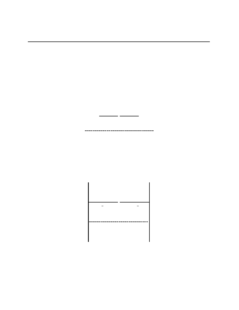
Chapter 4.1

A separating equilibrium is one in which all the different types of Senders take differ-

ent actions, thereby separating themselves from each other. A pooling equilibrium is one
in which all the different types of Senders take the same action. The only Nash equilibria
of the game just given are pooling equilibria, and all of them are sequential.

One of the sequential equilibria of the previous game is still a Nash equilibrium, but is

not a pbe (therefore not sequential) in the following, changed version of the above game.

low

high

0.2

0.8

entrant

out

enter

incumbent

100

−25

−10

Same structure, less story

-10

The previous signaling game, Γ

, depends on x Nature picks player 1’s type to be either

or θ

with equal probability. Player 1 then picks either up or down. If 1 picks up after

Chapter 4.1

either θ, the game is over with payoffs (x, 20) and (3, 15). If 1 every plays down, 2 picks
between a, b, and c without knowing which θ occured. The rest of the payoffs for Γ

are as

given in the following extensive form.

4.1.5

Spying games

One of the interesting aspects of information is who has it.
A simple case

Achieving coordination is often crucial. One way to achieve coordination in two person

strategic situations is to have one player “spy” on the other. This pair of games is designed
to get some of the simple implications of the possibility that one player may choose to
expend the effort to spy on the other in a two person coordination game. The specific
coordination game to be considered is

With the spying option, the game is altered so that player 2 can, before making their

choice, pay a utility cost of s > 0 and learn what 1 has done. Specifically, the game is

− s

spy

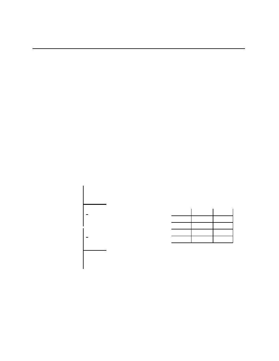
Chapter 4.1

Okay, time for a trick question — how many strategies does 2 have in the canonical nor-

mal form version of the previous game? To figure this out, note that 2 has three information
sets, and has 2 choices at the left one, 3 choices at the middle one, and 2 at the right one.
This means that 2 has 2

· 3 · 2 = 12 complete contingent plans.

Exercise: write out the 2

×12 canonical normal form, notice that there are a lot of duplicate

strategies, call any pair of strategies that give everyone the same payoffs equivalent, and find
the equivalence classes. Count equivalence classes as single strategies, and give an extensive
form game having the resulting, smaller, normal form game as its canonical form.

Going to war as a signal

With probability 2/3, country 1’s secret military research program makes their armies

deadlier (i.e. giving higher expected utility in case of war through higher probability of
winning and lower losses), and with probability 1/3 the research project is a dud (i.e.
making no change in the army’s capacities). Knowing whether or not the research program
has succeeded, country 1 decides whether or not to declare war on or to remain at peoce
with country 2. Country 2 must decide how to respond to war, either f ighting or ceding
territory, all of this without knowing the outcome of 1’s research program. With payoffs,
one version of the game tree is:

deadly

dud

war

peace

···

··

−6

(p, p)

(9, 6)

(p, w)

(4, 6)

(10, 4)

(w, p)

(7,

−2) (11, 2)

(w, w)

(2,

−2) (12, 0)

Let us modify the previous game by adding an earlier move for country 2. Before country

1 starts its research, country 2 can, at a cost s > 0, insert sleepers (spies who will not act for

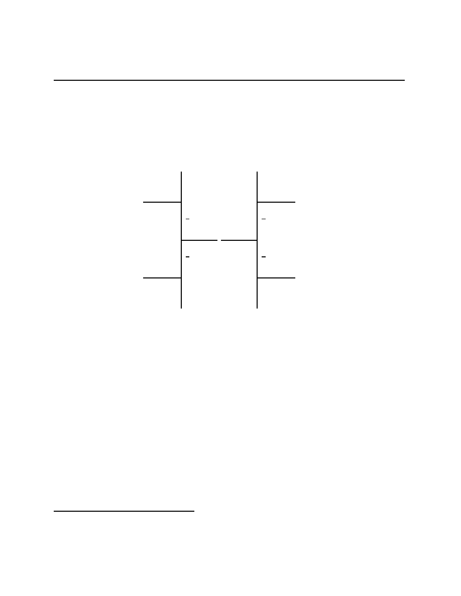
Chapter 4.1

years) into country 1. Country 1 does not know whether or not sleepers have been inserted,
and if sleepers are inserted, country 2 will know whether or not 1’s military research has
made them deadlier. One version of the game tree is:

spy

not

deadly

dud

deadly

dud

war

peace

war

peace

· · · · · · · · · · · · · · · · · · · ·

···

··

−6

− s

−6 − s

− s

−6

− s

Later, we will evaluate, in the context of these two versions of this game, the statement,

“When spying is cheap, it lowers the probability of war.”

Once again, you should know how to find the canonical, normal from strategy sets for this

game. Player 1 has to make decisions at two information sets, and has two actions available
at each one, meaning 4 strategies. Player 2 has to make decisions at four information sets,
and has two actions available at each, therefore has 2

= 16 complete contingent plans.

Notice that many of them are redundant — if 2 decides not to spy, then all of the decisions
on the left side of the tree do not matter to anyone’s utility. The decisions that would be
made there matter to the equilibrium, but not to the utilities in the normal form.

4.1.6

Other extensive form games that I like

The first two games are called “horse games” because the game tree looks like a stick figure
horse,

not because it was inspired by stories about the Wild West.

As drawn by a theoretical economist to be sure.

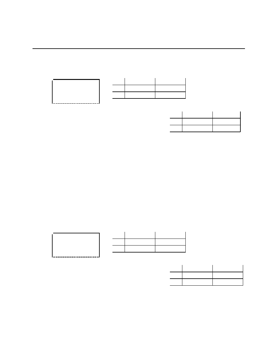
Chapter 4.1

A horse game

(20, 15, 30)

(10, 9, 0)

(15, 40, 10)

(20, 15, 30)

(30, 20, 1)

(0, 50, 0)

Imagine that 1 and 2 are lawyers in a law firm. 1 must decide whether to hand the case

over to 2, the action A

, or to prepare it themselves, D

. If the case is handed to 2, she must

decide whether to go forward, D

, or leave the case alone, A

. The differing competences of

lawyers 1 and 2 leave 3 having different opinions about their options, say fighting or settling,
L

and R

. 3 is happiest if both 1 and 2 opt out, 2 would most like to prepare the case

herself and have 3 settle, etc.

The 3-person normal form representation of this game has two matrixes. 1 picks the

rows, 2 picks the columns, and 3 picks the matrix.
Exercise: Find the equilibria for this game.

Another horse game

(

)

(

)

(

)

(

)

(

)

(

)

(

)

(

)

Exercise: Fill in the payoffs for the normal form representation of this game, find the
equilibria, and figure out which of them are sequential.

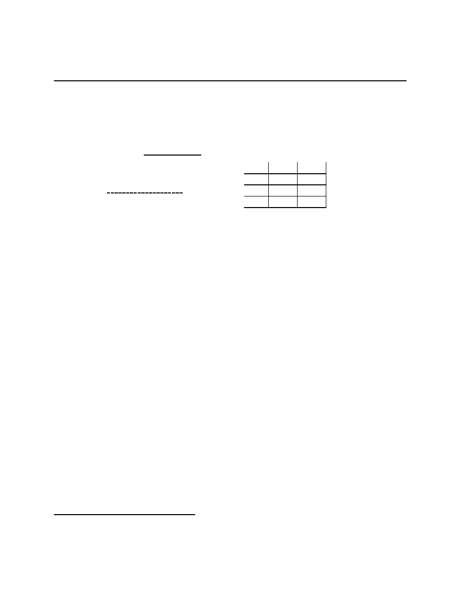
Chapter 4.1

A money-burning game
Here, player 1 can either opt out or play a coordination game. When player 1 lets player

2’s choice matter, this means that 1 has given up a sure payoff of 2. Following Dekel’s
insights, we sometimes think of that as burning money.

Out

(2, 9)

(5, 1)

(0, 0)

(1, 5)

Two of the equilibria in the coordination game are worse than opting out. Thus, when 1

gives to 2 the opportunity to move, 1 has publicly given up the worth of the outside option,
they have, in other words, burned some money. If you were 2 and knew that 1 had given
up the safe outside option, you might conclude something about what 1 must have done in
giving you the choice.

Two games without clocks

The following is a tale of envy and spite. In it, neither can have a clock. That should sound
a bit surprising, no mention of clocks was made in the previous games. Read on.

A Tale of Envy and Spite. In it, neither can have a clock. That should sound a bit

surprising, Two people, Bertrand and Cournot, who dislike each other rather strongly, are in
the habit of taking an evening stroll through the local marketplace. When approached by a
vendor selling a unique, one-of-a-kind silk tie, they may either accept or reject the offer. In
making this decision, they do not know whether or not the vendor has already approached
the other and been rejected. However, they do know that it is equally likely that they are
the first to be approached, and that, if they are first and reject the tie, the other will be
approached.

Both like the tie, but both dislike accepting a tie the other has rejected, and both dislike

having the other also reject a tie they have rejected (such is envy and spite). With payoffs,
one game tree for this situation is, with N being Nature, or Chance,

I don’t entirely agree with this logic, but it is very popular.

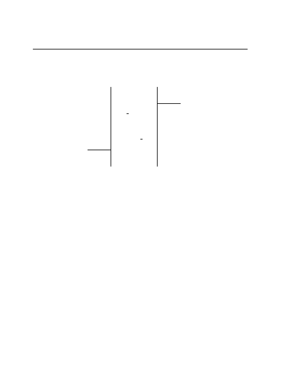
Chapter 4.1

· · · · · · · · · · · · · · · · · · · ·

−1

Bertrand

Cournot

rej

acc

Problem 4.2 Give the normal form for this game, find all the equilibria for this game, and
find the set of normal form correlated equilibria.

The correlating device is, by assumption, independent of Nature’s move. Suppose instead

that the recommendation made by the correlation device can be dependent on Nature’s choice.
Formulate and solve for the equilibrium outcomes of resulting game. (Hint: The equilibria
of games with this kind of extensive form correlation are called ‘communication equilibria’
by Forges and Myerson.)

So, why might this be called a game without a clock? One way to answer is to suppose

that both Cournot and Bertrand start their evening stroll at 6:30 p.m. every evening. If they
are approached at 6:31, then they are pretty sure that they are the first to be approached.
If they know something about the arrival time and the degree of hustle of the vendor, then
not being approached until 7:30 might be a pretty clear indication that they are the second
to be approached. In either of those cases, the description of the uncertainty given in the
game tree is no longer correct.

A New Chair. The Department of Economics at Moo U. needs a new chair. The Dean has
narrowed her choices down to two possibilities, Professor BillyBob and Professor Cuthbert.

Chapter 4.2

The existence of a chair is a public good. The benefits to both professors of having a chair
are normalized to 1, so that both receive utility b = 1 if either becomes chair. The costs
to the Professors are private information, independently distributed, and taking the values
c = 1/3 and c = 2/3 with probability

each. Costs are borne only by the Professor who

becomes chair so that if, say, BillyBob becomes chair, the utilities to BillyBob and Cuthbert
are (1

− c

BillyBob

, 1). If neither becomes chair, both receive utility of 0.

The Dean picks one of the two professors at random and offers them the chance to do

the chore of being chair. If the first professor turns the job down, the Dean offers it to the
second professor. If the second professor turns them down, the Dean loses patience and
appoints an incompetent third professor who gives benefits b = 0 to both BillyBob and
Cuthbert. A striking aspect of this game is that, in making their decision of whether or not
to accept, neither BillyBob nor Cuthbert know if they are the Dean’s first choice, or if the
Dean has already been refused once.

Problem 4.3 Carefully draw a tree representing the game between BillyBob and Cuthbert.
[This could get a little tricky. There are 8 equally likely choices for Nature/Mysterio, each
choice can be represented as a vector (c

, c

, i) where c

∈ {L, H} is BillyBob’s costs,

∈ {L, H} is Cuthbert’s, and i ∈ {B, C} is the Professor who is offered the job first. Also,

each information set for each player should contain 4 nodes.]

Solve for all of the pure strategy equilibria of the game you just gave.
Which, if any, of the pure strategy equilibria are sequential?

4.2

Formalities of extensive form games

Here they are, we’ve now seen many extensive form games and have a sense of the kinds of
things they model. Now we need to give the rules we’ve been living by.

1. Nodes: These are the places in game trees where “things happen,” either someone

(including Nature) makes a choice, or the game ends. Nodes are either the heads or
tails of vectors in the pictures above (and below). The nodes that are only at the tails
of vectors are called terminal nodes, these are the ones where games end.

X will be

used to denote the set of nodes for a game.

2. Arrows: The possibility of moving from one node to another node is represented by

arrows in the diagram. There are at least two ways to represent these arrows. First,
as a set of ordered pairs with the first one being the head of the arrow and the second
being the tail, that is, K

⊂ X × X is a partial ordering. We are going to have to

assume that K is a tree with a root, i.e. you cannot go in cycles, no node is its own
predecessor, and only one node has no predecessor.

Chapter 4.2

3. Immediate predecessors: The arrows can also be represented by a function p :

X →

{X, ∅} that maps each node in X to its immediate predecessor.

4. The origin: By assumption, there is only one node with no predecessor, it is called the

root or the origin, sometimes denoted by

o , sometimes by an open circle, sometimes

by a filled in circle.

5. Immediate successors: The immediate successors of a node x is s(x) = p

−1

(x).

6. Predecessors: Iteratively applying p(

·) gives the set of all predecessors, e.g. p(r) = x,

p(p(x)) = p(

o ) = ∅, so the set of all predecessors of the node r is {x, o }.

7. Successors: Iteratively applying s(

·) gives the set of all successors.

8. Terminal nodes and decision nodes: The terminal nodes are T =

{x ∈ X : s(x) = ∅}.

All other nodes,

X\T , are called decision nodes.

9. Who plays where: The player partition P is a partition of

X\T into I + 1 sets,

, P

, . . . , P

. At x

∈ P

, player i is the one to choose an action. Player 0 is Chance

or Nature.

10. Information partition: It matters very much what one knows when one makes a choice,

and this is the function of the information partition. To each P

, there is a partition

of P

, the elements of U

are called the information sets of player i. The idea

is that player i cannot distinguish between points in an information set in U

. This

means that player i’s choices cannot vary across different parts of their information
set, the second condition just below. In the pictures, information sets are represented
dashed lines connecting decision nodes.

The partitions U

must satisfy two conditions,

(a) For every terminal node z, the set of predecessors of z intersect any information

set at most once. [This condition is repeated as the first condition in the Perfect
Recall assumption below.]

(b) All nodes in an information set must have the same number of successors.

11. Actions: The last two conditions are related to the choice of actions available to the

players. In the game above, player 1 has two actions at the information set H =
{o } ∈ U

, the set of available actions, A(H), is

{Push

, Wait

}. At the information

set H =

{x, y} ∈ U

, A(H) is the set

{Push

, Wait

}. The implications of 2 choosing

a particular action depend on where in

{x, y} the player actually is — if at node x

Push

and Wait

lead to terminal nodes r or s, if at y, they lead to t or u.

Chapter 4.2

For any decision node x, let H(x) denote the information set containing x and let A(x)
be a set of actions available at x. At decision nodes x, we assume that if H(x) = H(x

then A(x) = A(x

) so that A(H) is well-defined for any information set H. Further,

we assume that at every decision node x, there is a one-to-one correspondence between
elements of A(x) and s(x), the immediate successors of x. The interpretation is that
at H(x)

∈ U

, player i chooses some a

∈ A(H(x)), and this leads to the corresponding

node in s(x).

Now we can explain the conditions (a) and (b) on the information partitions.

(a) If this condition is violated, then not only does player 1 not remember what he’s

chosen in the past, s/he may not remember having chosen.

(b) If two nodes, x

6= x

, in an information set H

∈ U

had different numbers of

successors, then i’s decision problem at the two nodes differ. Since we want to
assume that when people choose, they choose from a known set of options, they
would need to know whether are at x or at x

. But x, x

∈ H ∈ U

represents i

not being able to distinguish the two.

12. Perfect recall: We assume that the players never forget something they once knew —

if they observe an action by someone else or take an action themselves, they will never
arrive at a later point in the game at which they do not know all the consequences of
the observed or taken action.

Formally, two conditions must hold, the first was given above:

(a) If x and x

are in the same information set for a player i, H(x) = H(x

), then x

is neither a predecessor nor a succesor of x

(b) If x

6= x

are in the same information set for a player i, H(x) = H(x

), x

a predecessor of x belong to one of i’s information sets, and a

is the action at

H(x

) that leads (eventually) to x, then there must be a predecessor, y, to x

that belongs to H(x

) such that a

is the action taken at y on the way to x

. (If i

cannot distinguish between x

6= x

, then it had better not be the case that i had

information distinguishing x and x

at any predecessor of x at which i chose an

action.) The left hand game in Figure 2 violates this condition if we take x = x

= x

, the right hand game violates this condition if we take x

∈ {y

, y

} and

∈ {y

, y

Chapter 4.2

o 1

Figure 2

13. Strategies: A pure strategy for i is a mapping from the H

∈ U

to the associated

A(H). The H’s in U

are the possible contingencies that may arise, the places at

which i may need to choose an action. To rephrase, a strategy for i is a complete
contingent plan, a list of what will be done at each and every contingency, that is,
at each possible H in U

. A mixed strategy is a probability distribution over pure

strategies.

This concept of a strategy as a complete contingent plan turns out to be amazingly
hard for many people, but it is crucial. I think this is because, for the most part, we
go through our lives figuring out what we will do when we get to the decision point,
crossing the bridge when we get to it colloquially. Go back and review the Bridge
Crossing Lemma. Once you’ve done that, take a look at the following examples.

(a) In the first spying game, 1 moves at only one information set, picking either

L or R. This means that 1’s set of pure strategies is

{L, R}. 2 moves at three

information sets, the one directly after 1 has moved, the one where 2 has chosen to
spy and learned that 1 pick L, and the one where 2 has chosen to spy and learned
that 1 pick R. Reading the information sets from left to right, the 12 = 2

· 3 · 2

strategies are

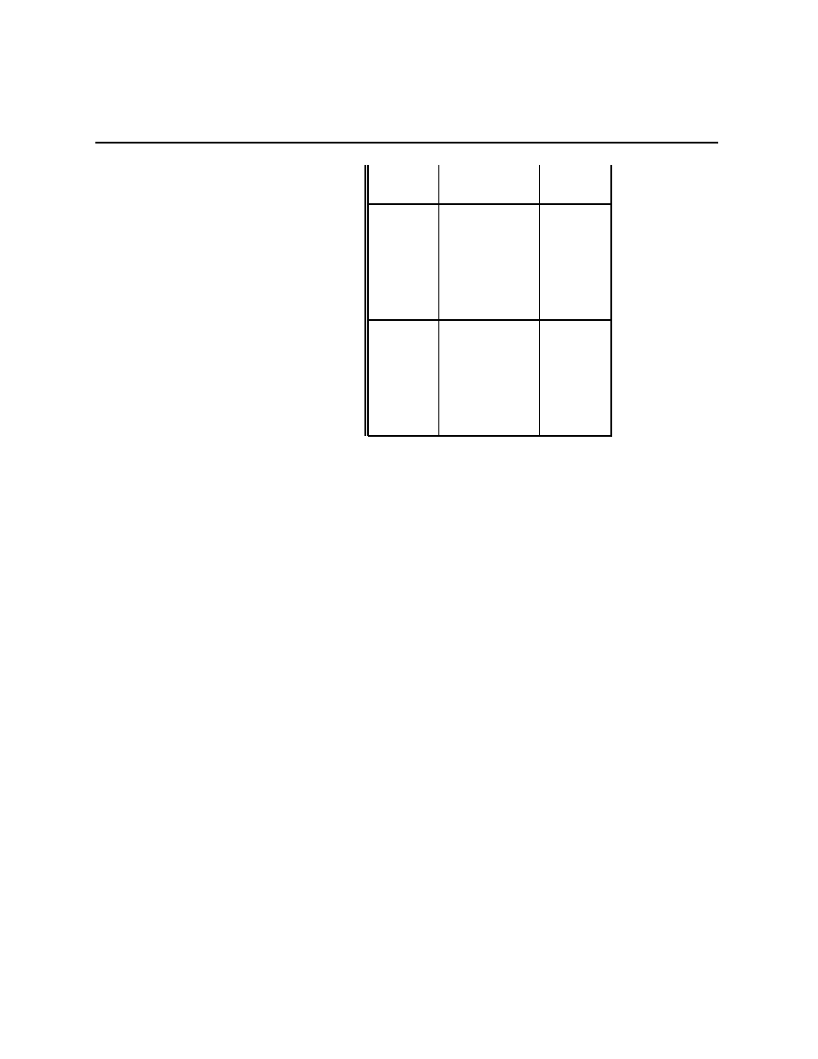
Chapter 4.2

2’s info set

spying

1 has moved

spying

found L

found R

spy

(b) In the Felicia game, her pure strategies specify a complete contingent plan, that

is, a plan that tells what she will do in either the high or the low damages case.
Reading from left to right in that game tree, the four strategies are (D

, D

), (D

, D

), and (D

, D

). The Acme pure strategies are also complete

contingent plans, they specify what they will do when faced with either a H or
a L claim, (a

, a

), (a

, r

), (r

, a

), (r

, r

sets, making one of 2 choices at each one, so 1’s set of pure strategies has 4
elements. 2 moves at 4 different information sets, and has 2 choices at each one,
hence has 2

= 16 pure strategies.

14. Outcomes: Given a vector s = (a

)

i∈I

∈ A = ×

i∈I

of pure strategies (including a

pure strategy for Nature), there is a unique terminal node,

O(s) that will arise, that

is,

O : S → T . The outcome associated with a mixed strategy σ is denoted O(σ) and

is the image of σ under the mapping

15. Utilities: Associated with every terminal node z is a utility u(z). These are given as

vectors at the terminal nodes in the picture.

16. Equilibrium: A vector σ

∗

is an equilibrium if

(

∀i ∈ I)(∀a

∈ A

)[u

(

O(σ

∗

))

≥ u

(

O(σ

∗

))].

17. The normal (or strategic) form: Given an extensive form game, Γ, let A

denote i’s set

of pure strategies. Define v

(s) = u

(

O(s)). The normal form for Γ is (A

, v

)

i∈I

. That

Chapter 4.3

is, the normal form lists each player’s pure strategies and assigns utilities through
the outcome function. Thus, the definition of equilibrium just given is simply the
definition of an equilibrium of the normal form game. Sometimes this is called the
canonical normal form to distinguish it from some other kinds of normal form games
that we’ll get to later.

18. The agent normal form: We start with an extensive form game Γ having player set

I. Each i

∈ I has a collection U

of information sets. For each H

∈ U

, split i into a

component personality, i

Specifically, pretend that each i

is a separate person,

but, and this is crucial, pretend that their utility at z, u

(z), is equal to u

(z).

19. Behavioral strategies: In the agent normal form, randomization by the (i

)

H∈U

stochastically independent. This independent randomization over the A(H) is called a
behavioral strategy. A behavorial strategy gives a distribution over the pure strategies.
Kuhn’s theorem says that any distribution over the pure strategies can be replaced
by a strategically equivalent behavioral strategy. This means that any equilibrium σ

∗

gives rise to an equivalent vector of behavioral strategies, b

∗

, which must also be an

equilibrium. It is usually much easier to use behavioral strategies, and you will quickly
become adept at using them.

Problem 4.4 What is the dimension of the space of mixed strategies in the first spying
game? What is the dimension of the space of behavioral strategies.

4.3

Extensive form games and weak dominance argu-
ments

The time has come to start solving these games. There are too many equilibria, sometimes
“weak dominance” arguments can get rid of some of them.

4.3.1

Atomic Handgrenades

The first game we will solve is called Atomic Handgrenades, sometimes it is called the
Chain Store paradox. To remind you, you are approached by a fellow carrying a certified
atomic handgrenade.

He says, “Give me 20$ or else I will explode this small thermo-

nuclear device.” Your choice is whether or not to give him the 20$. One (not the only)
representation of this situation has your two strategies being “Give 20$” and “Don’t Give

This has the makings of a really bad tv show, but there are good reasons to do this.

Or suffer the consequences, sleepless nights and frustration.

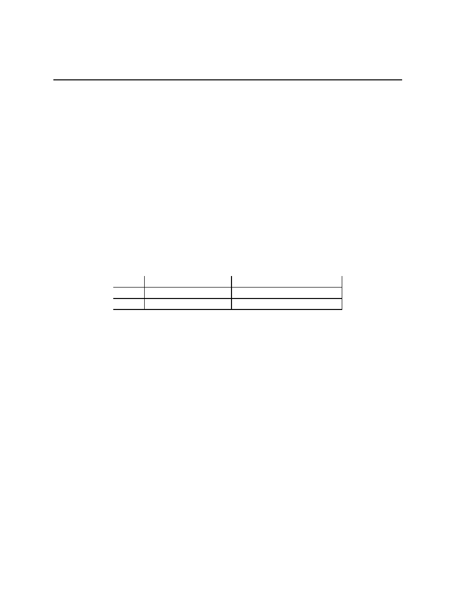
Chapter 4.3

20$”. The fellow’s strategies are “Blow up hand-held thermo-nuclear device if not given
20$” and “Don’t blow up hand-held thermo-nuclear device if not given 20$”. These are
strategies that have conditional clauses in them. The extensive form representation of the
game is (where

−y −20):

−20

−y

Atomic Handgrenades (redux)

The (canonical) normal form representation of Atomic Handgrenades is

Blow up if not given

Don’t blow up if not given

Give

(

−20, +20)

(

−20, +20)

Don’t

(

−y, −y)

(0, 0)

Note that there are exactly 2 equilibria for this game, and this is the first finite game in

which we’ve had anything but an odd number of equilibria. There is a reason for that, but
we would need more of a particular kind of mathematics than I am willing to wade through
to prove this kind of result. Further, since most of our interest is going to be in extensive
form games, the conditions guaranteeing an odd number of equilibria are usually violated.

It is embarassing to have two such different equilibria. Remember, we are trying to tell

stories about why things happen. Saying that either the bluff will work or it won’t is, in
modern parlance, “lame.”

Problem 4.5 Give the normal form for Gianni Schicchi and show that it too has 2 equi-
libria.

4.3.2

A detour through subgame perfection

This is a topic of some historical importance. Notice that Atomic Handgrenades has a proper
subgame, Γ

that starts at 2’s decision node. One could ask, as a matter of general principle,

that equilibrium in Γ, when restricted to Γ

, is an equilibrium. Such an equilibrium is called

subgame perfect.

Chapter 4.3

This is a fairly strong requirement, it requires that bluffing not happen in equilibrium.

This gets us what we want in this game, a unique “acceptable” equilibrium. However, there
are games Γ

having subgames that are equivalent (in very strong senses) to other games Γ

without subgames. The choice is either to abandon subgame perfection or to abandon the
equivalence of games. I’ll abandon subgame perfection as a theoretical construct without
much regret. However, since it’s an implication of theoretical constructs that we will accept,
you might as well know how to use it.

Problem 4.6 Two firms compete by producing quantities q

and q

of a homogeneous good,

and receiving profits of the form

, q

) = [p(q

+ q

)

− c]q

where p(

·) is the inverse market demand function for the good in question. Assume that

p(q) = 1

− q and that 0 ≤ c 1.

1. (Cournot competition) Suppose that the firms pick quantities simultaneously. Find the

unique equilibrium.

2. (Stackelberg competition) Suppose that firm i picks q

, which is then observed by firm j

before they pick q

. Find the set of equilibria for this game. Find the unique subgame

perfect equilibrium (called the Stackelberg equilibrium).

3. Find the profit rankings of the Cournot and the Stackelberg equilibrium.

Problem 4.7 A software designer, s, and a marketer, m, form a partnership to which
they contribute their efforts, respectively x

≥ 0 and y ≥ 0. Both have quasi-linear utility

functions, u

= $

− x

and u

= $

− y

, where $

and $

are monies received by s and m

respectively.

The twice continuously differentiable, strictly concave profit function π satisfies

(

†)

π(0, 0) = 0, and (

∀x

◦

, y

◦

> 0)[∂π(x

◦

, y

◦

)/∂x > 0, ∂π(x

◦

, y

◦

)/∂y > 0].

The profit function need not be symmetric, that is, it may happen that π(x, y)

6= π(y, x).

Consider the following three scenarios:

(A) Side payments are possible, and the Nash bargaining solution with threat point (u

, u

) =

(0, 0) determines the outcome.

(B) Neither effort nor sidepayments are legally enforceable, the partners choose their efforts
simultaneously, and share the profits equally.

Chapter 4.3

(C) Neither effort nor sidepayments are legally enforceable, and the partners share the profits
equally. However, the software designer chooses her effort before the marketer chooses hers,
and the marketer observes the designer’s effort before choosing her own.

1. Give conditions on π(

·, ·) above and beyond (†), the weaker the better, so that both the

software designer and the marketer strictly prefer (A) to (B). Prove your result.

2. Give conditions on π(

·, ·) above and beyond (†), the weaker the better, so that the

software designer strictly prefers (C) to (B). Prove your result.

3. Show that if, in addition to (

†), ∂π(0, 0)/∂x > 0 and ∂π(0, 0)/∂y > 0, then there is a

unique, strictly positive solution in scenario (B).

4. Show that if π(

·, ·) is homothetic, then the solution (x

, y

) in scenario (A) is a linear

multiple of any solution (x

, x

) in scenario (B). Under what conditions is the multiple

larger or smaller than 1?

We will talk about subgame perfection as weak dominance in agent normal form games

below. Weak dominance and iterated weak dominance is more generally applicable than sub-
game perfection. Remember throughout, arguments for weak dominance implicitly include
arguments against bluffing.

Problem 4.8 (The Rotten Kid Theorem) First, the child picks A

≥ 0. This gives rise

to incomes I

(A) and I

(A) for the child and parent respectively. Second, the parent observes

, I

) and chooses a bequest, B

∈ R, to leave for the child. The child’s utility is U(I

+B),

the parent’s is V (I

− B) + kU(I

+ B), k > 0. The usual strict concavity, differentiability,

and interior solution conditions hold for I

(

·), I

(

·), U(·), and V (·). In the unique subgame

perfect equilibrium of this game, A

∗

solves the problem max

A≥0

(A) + I

(A)). [What is

striking is that the possibility of being left a bequest by soft-hearted parent makes the child
behave perfectly admirably, even if they’re really rotten, that is, even if they do not care in
the least about their parent’s utility.]

Problem 4.9 Player 1 moves first, either choosing to play a 2

× 2 game with player 2, or

giving 2 a single choice. After 2’s single choice, the payoffs are (3, 0) or (2, 1). The 2

× 2

game has payoffs

Left

Right

(0, 3)

(1, 3)

Down

(2, 1)

(2, 0)

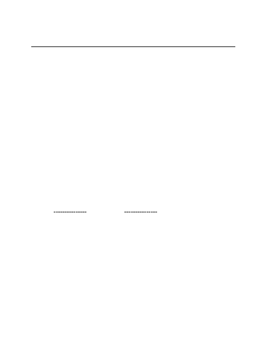
Chapter 4.3

1. Draw an extensive form representation of this game in which there are two subgames,

one at the beginning of 2’s single choice and one at the beginning of the 2

× 2 game.

Solve for the subgame perfect equilibria of this game.

2. Write out the (canonical) normal form for this game. Solve for any and all weakly

undominated equilibria in both forms. You should find subgame perfect equilibria that
are not weakly undominated and weakly undominated equilibria that are not subgame
perfect.

3. Write out the agent normal form for this game. Solve for the weakly undominated

equilibria of the agent normal form of this game. You should find that the subgame
perfect equilibria are now exactly the weakly undominated equilibria.

4.3.3

A first step toward defining equivalence for games

A more important observation is that the same normal form game arises from very different
extensive form games. Having T (for Top) and B (for Bottom) replacing the strategies
“Give” and “Don’t” above, L (for Left) and R (for Right) replacing the strategies “Blow
up if not given” and “Don’t blow up if not given” consider the following two games.

−20

+20

−20

+20

−y

−20

+20

−y

−20

+20

These last two extensive form games have the same normal form and the same equilib-

rium set as Atomic Handgrenades. As a first take on the equivalence of games, let us agree
that two games with the same canonical normal form are equivalent. For all three of these
equivalent games, the equilibrium set is

{(T, L), (B, R)}.

When we look at the (T, L) equilibrium in the Atomic Handgrenades version, it requires

that player 2 be playing the strategy “If we should arrive at the point x where I must
choose between blowing everything up and not blowing everything up, I will choose to blow
everything up.” This seems to be a rather unlikely strategy for 1 to seriously believe that 2

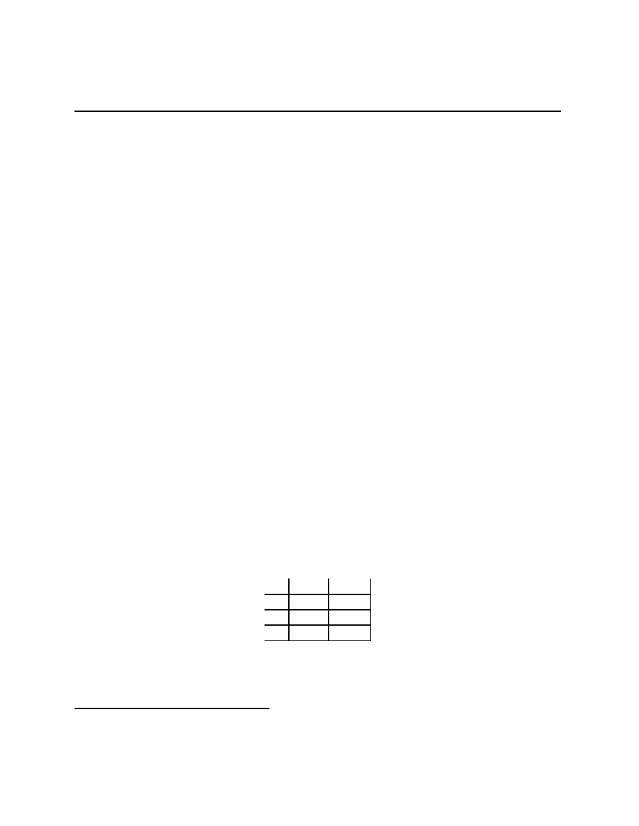
Chapter 4.4

will contemplate,

so maybe we should not believe in the (T, L) equilibrium. While this is a

good intuition, but it doesn’t help in any of the equivalent games because there is no point
like x at which we can say that 1 would never believe that 2 is contemplating something
foolish.

There is an argument as to why the strategy L is a bad one for 1 to think that 2

is playing, and the argument works in all four forms of the game. It has to do with the
observation that, no matter what strategy 1 is playing, 2 is always at least as well off playing
R as playing L, and for some strategies that 1 might play, 2 is strictly better off playing R
instead of L. This is called weak dominance, and perfectly reasonable people believe that
weakly dominated strategies are not used.

4.4

Weak dominance arguments, plain and iterated

A strategy σ

∈ ∆

strongly dominates t

∈ A

(

∀σ

∈ ∆)[u

(σ

\σ

) > u

(σ

)].

No strongly dominated t

can be in the support of any equilibrium (for finite games).

A strategy σ

∈ ∆

weakly dominates t

∈ A

(

∀σ

∈ ∆)[u

(σ

\σ

)

≥ u

(σ

)] and

(

∃σ

◦

∈ ∆)[u

(σ

◦

\σ

) > u

(σ

◦

)].

Comment: Splitting agents, as we do in agent normal form games, changes the set of
strategies and the set of weakly dominated strategies. Go back and look at Problems 4.9.
Then do the following problem.

Problem 4.10 (Kohlberg & Mertens, Figure 9) Consider the two player game

Left

Right

(2, 2)

(1, 1)

(2, 2)

(0, 0)

1. Show that (X, L) is the only undominated equilibrium of this game.

At least if the payoffs/preferences are as given.

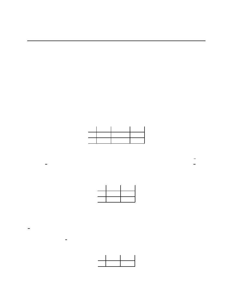
Chapter 4.4

2. Give an extensive form representation of the following game: Split agent 1 into 1

who picks whether or not to play Y and 1

who, if s/he has chosen not to play Y ,

picks between X and Z; have 2 pick L or R after 1

and 1

and in ignorance of those

choices.

3. In the extensive form game you have given, show that R is dominated for 2. Show

that in the extensive form game with R deleted, only Y is undominated for 1

In Atomic Handgrenades, R weakly dominates L, so that if we believe that weakly

dominated strategies are never used, then the only part of the equilibrium set that we are
interested in is (B, R). Weak dominance arguments get rid of some equilibria.

You might wonder why we allow mixed strategies in the definition of things that might

weakly dominate a given t

. Consider the following game.

(9, 4)

(30, 1)

(6, 0)

(110, 1)

(6, 4)

Neither strategy for 1 is weakly dominated. The strategy M is not weakly dominated by
either L or R, but it is strongly dominated by any σ

∈ ∆

satisfying σ

(L) >

and

(R) >

. The set of equilibria for this game is Eq =

{(T, L)} ∪ {(σ

, R) : σ

(B)

≥

Now suppose that we look at the game in which M is removed because it will never be

played. This gives the game

(9, 4)

(6, 0)

(6, 4)

and in this game T weakly dominates B for 1, but none of 2’s strategies are weakly domi-
nated. We considered only a subset of ∆ as possibilities, and new weak dominance relations
appeared. For this game, the set of equilibria is (again) Eq =

{(T, L)} ∪ {(σ

, R) : σ

(B)

≥

Now suppose that we look at the game in which B is removed. None of the equilibria in

{(σ

, R) : σ

(B)

≥

} make any sense in this game because they are putting positive mass

on strategies that have disappeared. The new game is

(9, 4)

(6, 0)

Chapter 4.5

In this game 1 has no weakly dominated strategies, but R is strictly dominated for 2. Remov-
ing R leaves the only possible actions being (T, L). Iteratively deleting weakly dominated
strategies has reduced the set of equilibria.

Problem 4.11 Show that in the Cournot game with linear demands, iterated deletion of
weakly dominated strategies leads to the Cournot equilibrium.

In the following game, player 1 has an outside option, a safety point if you will. In the

extensive form game, if player 2 gets to play, it means that 1 has forsaken her/his outside
option. One could argue that this means that 2 should believe that if s/he gets to play, it is
because 1 believes that the equilibrium that 1 and 2 will play together is better for 1 that
the outside option. This is called a “money burning” game because player 1 has forsaken
something expensive, an example of forsaking something expensive is burning money. The
iterated deletion of weakly dominated strategies that delivers this conclusion also applies to
the version of the game in which 2 moves first and then 1 picks, not knowing what 2 has
picked.

Problem 4.12 Consider the following version of the money-burning game, Γ,

Out

1. Give the normal form for Γ.

2. Give the extensive form of this game in which 2 move first.

3. Find Eq(Γ).

4. Find the subset of Eq(Γ) that survives iterated deletion of weakly dominated strategies.

The above iterative procedure made use of dominance relations that only appear when

a subset of ∆ is being considered. This idea of dominance relative to a set turns out to be
very useful, and we will return to it after we take a detour through some of the best known
applications of weak dominance arguments.

Chapter 4.5

4.5

Mechanisms

Suppose somebody, call them a principal, wants to hire someone else, call them an agent,
to do a particular job. A possible complication is that the principal cannot observe, at least
not at any reasonable cost in time or money, exactly how the agent does the job. Another
possible complication is that the principal doesn’t know everything about the job that the
agent knows. However, the principal does observe the final outcome. The principal wants
to design a reward schedule for the agent, a mechanism if you will, that depends on the
observable final outcome, and that induces the agent to behave as the principal desires.

For example, the owner of a factory (the principal) may hire a manager (the agent) to

run the factory while the principal runs off to the South Pacific. It is too costly for the
principal to watch what the agent does from Tahiti. However, each quarter the principal’s
accountant calls and tells the principal the realized profits. Now, profits are presumably
related to the agent’s actions, but they also have a random component. This is a peculiar
market, the principal is buying the services sold by someone else, but the exact services
are not specified in the contract. Here the mechanism is a wage schedule depending on the
observable profit.

For another example, the principal sees a doctor or a lawyer (agent) when something is

wrong. Often, the extent and treatment for the problem are not known to the principal and
only probabilistically known to the agent. The principal eventually observes the outcome,
that is, when/if the problem goes away. This too is a peculiar market, the principal is asking
the agent what is needed and then buying the needed services from the agent. In the doctor
example, the wage schedule should depend on the health outcome.

For yet another example, people differ in their real willingness and ability to pay for

public goods. Public goods should be offered if the sum, over the affected people, of the
willingness to pay is greater than or equal to the cost of the public good. However, if actual
payment depends on reported willingness to pay, people have a motivation to “free ride,”
that is, to say that the are less willing to pay than they truly are in order to receive the public
good at less cost to themselves. Here, one invents a rule or mechanism for turning reported
willingnesses to pay into a decision about the public good. Given the mechanism/rule, the
people best respond. In particular, they don’t play weakly dominated strategies. Here,
the principal is an abstraction sometimes thought of as society, there are many agents, and
society, in the guise of the economist writing down the model, wants to get a particular kind
of outcome. Some specific models are in order.

4.5.1

Hiring a manager

The principal offers a contract to the agent. The contract specifies what reward or wage
the agent will get as a function of the observable outcome, say profit — S

is the set of

Chapter 4.5

functions π

7→ w(π). The agent examines the contract, w(·), and either decides to decline

the job offer, or accepts the offer and chooses a managerial behavior, b

∈ B — S

is the set

of functions from S

{decline} ∪ B. If a point in B is chosen, then a random profit, Π

, is

realized. The expected utilities when the job offer is not declined are E u

(Π

− r(Π

)) and

E u

(r(Π

), b). The principal’s utility depends only on the difference between the realized

profit and the wage they pay, the agents utility depends only on the wage they receive and
their choice of managerial behaver. If the job offer is declined, the expected utilities are u

and u

Just as in Atomic Handgrenades, the manager could bluff, saying that s/he won’t take the

job unless offered a very large salary schedule, one that guarantees more (in expected utility)
than u

. However, when offered something more reasonable, by which I mean some lower

wage schedule offering an expected utility greater than u

, declining is a weakly dominated

strategy. Thus, in looking at an equilibrium for this game, we can proceed in two stages:
first, figure out 2’s best responses to different w(

·)’s; second, figure out the highest E u

a function of w(

·) coupled with best responses by 2.

We are going to start with the simplest case: B =

, b

} where l and h stand for low

and high respectively, the possible profit levels are

{π

, π

}, π

< π

, the probability of π

conditional on action b

being taken is P (π

) = α, the probability of π

conditional on

action b

being taken is P (π

) = β, and 0 < α < β < 1. Also, suppose that u

is of the

form u(w)

− v(b) where u is concave in wages, where v(b

) < v(b

), and suppose that u

linear in profits minus wage payments.

Problem 4.13 For some values of the parameters of this game, the equilibrium involves the
manager choosing b

. Charaterize the equilibrium w(

·) for such equilibria. For other values

of the parameters of this game, the equilibrium involves the manager choosing b

. Show that

the corresponding equilibrium w(

·) involves performance rewards, that is, w(π

) < w(π

[You can use graphs to answer this question.]

Problem 4.14 Change the set of profit levels to

{π

< π

· · · < π

}, have P (π

) =

, P (π

) = β

where

M
m=1

, but otherwise leave the game un-

changed.

1. For some values of the parameters of this game, the equilibrium involves the manager

choosing b

. Charaterize the equilibrium w(

·) for such equilibria.

2. For other values of the parameters of this game, the equilibrium involves the manager

choosing b

. For such an equilibrium:

(a) Give the Kuhn-Tucker optimality conditions that must be satisfied by the equilib-

rium w(π

), m = 1, . . . , m.

Chapter 4.5

(b) Show that the equilibrium w(

·) may not involve performance rewards, that is,

w(π

) > w(π

m+1

) is possible.

/β

decreases in m, the equilibrium w(

·) involves performance

rewards.

3. Add an extra stage to this game — after observing π

, the manager can report any

m−k

≤ π

(say by overpaying a supplier), and wage depends on the reported π. Show

that in any equilibrium involving the manager picking b

, the equilibrium w(

·) involves

weak performance rewards, that is, w(π

m−1

)

≤ w(π

4.5.2

Funding a public good

A group of neighborhood families, i

∈ {1, . . . , I}, must decide whether or not to pool their

money to hire a morning crossing guard for a busy intersection that the children walking to
school must cross. The cost of a guard is C, which must be financed by family contributions,
t

. The set of feasible alternatives can be modeled as

X =

{x = (y, m

− t

, . . . , m

− t

) : y

∈ {0, 1}, t

≥ 0,

≥ yC},

where m

is family i’s initial endowment of money. Family i’s preferences are given by

(x, θ

) = θ

y + (m

− t

where θ

∈ Θ

{θ

, θ

} where 0 < θ

< θ

. The θ

are independent, and have probability

of being either θ

or θ

. The set of possible vectors of preferences is Θ with typical

element θ = (θ

, . . . , θ

)

∈ Θ = ×

i∈I

. We are going to assume that each family knows

their own θ

but not the θ

of any j

6= i. (Draw a tree here).

A social choice rule is a function f mapping Θ to X. Family i’s maximal willingness to

pay, p

, is the number that solves

+ (m

− p

) = m

because paying p

and having the public good (crossing guard) leaves them just as well off

as they are without the public good. In particular, p

= θ

. A social choice rule is ex post

efficient if for all θ such that

> C, f (θ) has y = 1, and if

< C,

f (θ) has y = 0.

The general form of a political decision process involves each family i picking an m

some set M

(“M” for Message). Since the M

at this point are rather abstract, this seems

to cover all of the relevant territory — M

might include canvassing the neighbors, putting

Chapter 4.5

up placards, calling city hall, sacrificing chickens to the traffic gods, whatever. However, we
think that contributions to the crossing guard fund are voluntary, so the M

should include

an m

corresponding to “i will make no contribution,” and if m

is played, then family i

makes no contribution. A strategy for family i a point in A

= M

{θ

,θ

}

. A vector s of

strategies gives a mapping from Θ to

i∈I

. A mechanism is a mapping,

M, from ×

i∈I

to allocations. Putting these together, each strategy gives a mapping from Θ to allocations.
Since allocations have associated utilities, s

7→ E u

(

M(s)), we have a game. Since a given s

leads to a distribution over the terminal nodes and it is E u that is maximized, the equilibria
for these games are sometimes called Bayesian Nash equilibria.

Since no-one can be forced to pay, the mechanism must have the property that for any

m with m

= m

, then i’s part of the allocation in

M(m) involves i not paying. One

interesting kind of question is whether or not there exist any mechanisms with the property
that the equilibrium of the corresponding game is ex post efficient. At first glance, this
seems impossibly difficult to answer, after all, there are no restrictions on the M

nor the

besides the existence of a “no pay” option. However, there is a result, called the Revelation
Principle, that allows us to study this question with some hope of success.

Some terminology: a social choice rule f (

·) is implemented by a mechanism M if

there is an equilibrium s

∗

such that

∀θ ∈ Θ, M(s

∗

(θ)) = f (θ). We are trying to answer the

question “Which social choice rules are implementable?”

Intuition: when a family of type θ

plays in a pure strategy equilibrium, s

∗

, they play

= s

∗

(θ

). We can, if we wish, interpret any given s

∗

(θ

) as if the family had said θ

Equivalently, we can imagine a mechanism that asks the family for their θ

and guarantees

that if told θ

, s

∗

(θ

) will be played. Since the mechanism delivers the same allocation, they

family is just as happy revealing their true willingness to pay.

It’s important not to get too excited here — everyone truthfully revealing their types is

possible, but only if it is part of an equilibrium. It is still the case that if revealing their type
hurts them, they won’t do it. In particular, everyone must have the option of not paying.

Formally, replace each M

with the simpler two point space, M

{θ

, θ

}, and define

a simpler mechanism,

(θ) =

M(s

∗

(θ)). Let f (

·) be the mapping from Θ to alloca-

tions induced by s

∗

and

M, equivalently, by truth-telling and M

, and let us examine the

implications for f (

·) of these strategies being an equilibrium.

First, it must be that case that

∀i ∈ I, E u

(f )

≥ w

. If this is not true, then s

∗

is not

an equilibrium because the family has the option of playing the strategy s

≡ m

, which

delivers an expected utility greater than or equal to w

. These conditions, one for each

∈ I, are called individual rationality (IR) constraints. Second, after seeing any θ

, the

expected utility to reporting θ

must be at least as large as reporting any θ

6= θ

. If

this is not true, then s

∗

is not an equilibrium, after all, one of the options with the original

mechanism is to play s

(θ

) = s

∗

(θ

), but it is an equilibrium to play s

∗

(θ

). In terms of f (

·),

it must be the case that for all i

∈ I, E u

(

(θ

\θ

))

≥ E u

(

(θ

\θ

)) for all θ

. These

Chapter 4.5

conditions are called incentive compatibility (IC) constraints.

The IR and IC constraints must be satisfied if f is implementable. If f satisfies the

constraints, then it is implementable by the truth telling strategies in the simpler game
described above. Therefore

Theorem 4.3 The social choice rule f (

·) is implementable if and only if it is feasible and

satisfies the IR and IC constraints.

Now the real work starts, what’s implementable?

Problem 4.15 Suppose that

> C >

and f (

·) is the unanimity rule, “hire the

guard and spread the cost evenly between the families only when all report θ

.” Show that

f (

·) is implementable but not generally efficient.

Problem 4.16 Suppose that f is the rule, “hire the guard and spread the cost evenly among
those reporting θ

only when the sum of the reported θ

’s is greater than C.” Is this

implementable? Efficient?

Problem 4.17 The following pivotal voter rule satisfies the IR and IC constraints, but
may not be feasible, and may collect more money than is needed to finance the project.

(θ

, . . . , θ

) =






(1, w

− θ

)

j6=i

≥ C,

(1, w

− (C −

j6=i

))

if C

− θ

≤

j6=i

< C,

(0, w

)

otherwise.

Let y

∗

(θ

, . . . , θ

) = 1 if

≥ C, 0 otherwise. Let ˜θ

−i

denote the random realization

of the type of families other than i. Define a class of transfer functions, mechanisms if you
will, depending on reported θ’s, by

(θ) =

−E

j6=i

· y

∗

(θ

, ˜

−i

) + h

(θ

−i

So far as equilibrium calculations are concerned, the h

(θ

−i

) cannot affect anything, this

from Lemma 1.4. When each i maximizes the first term, they are maximizing a term that
we can think of as containing the sum of their externalities on other players, assuming that
the other players truthfully reveal their own θ

. When all players do this, the mechanism

satisfies the IC constraints, by fooling with the h

(

·), it is also possible to take care of

feasibility and budget balancing.

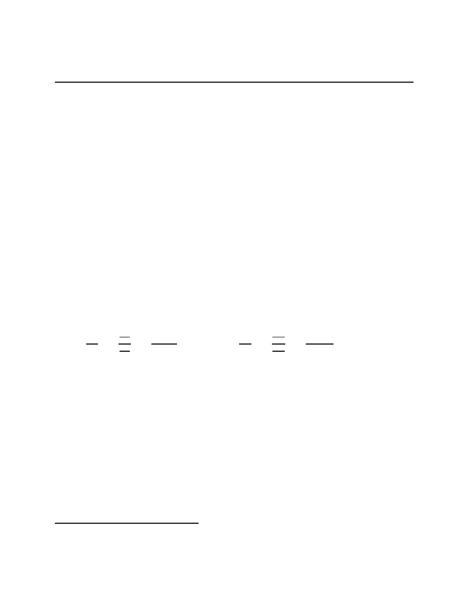
Chapter 4.5

4.5.3

Monopolist selling to different types

Roughly 20% of the consumers of peanut butter buy 80% of the peanut butter that is sold.
Roughly the same is true for hard liquor and wine. These are goods that are sold in larger
and smaller quantities, and it is usually the case that the per unit price is cheaper for the
larger quantities.

One explanation for this phenomenom is that the per unit packaging cost

is smaller for the larger containers, after all, volume goes as the cube of dimension while
packaging goes as the square. However, that is too prosaic an explanation for our present
tastes and purposes, so we are going to look for another explanation.

Suppose that there are two types of consumers of peanut butter, good x, and that they

are described by the two utility functions,

(x, w) = r

v(x) + w, u

(x, w) = r

v(x) + w,

where 0 < r

< r

, v(

·) is a differentiable, strictly concave, strictly increasing function

satisfying v(0) = 0 (a harmless normalization), lim

x→∞

(x) = 0 (the consumer eventually

grows tired of peanut butter), lim

x↓0

(x) > c where c is the marginal cost of producing

peanut butter (the type l consumer’s marginal utility of peanut butter is larger than the
marginal cost of peanut butter if they have nearly none of it), and w represents wealth to
spend on other items in the consumer’s life. In the x-w plane, the slopes of the indifference
curves are

−

∂u

∂x

∂u

∂w

−

(x)

−r

(x),

−

∂u

∂x

∂u

∂w

−

(x)

−r

(x),

so that the indifference curve of the h type through any point (x, w) is strictly steeper than
the indifference curve of the l type through the same point. This is the famous single-
crossing property — the indifference curves of the different types cross at most a single
time.

Before advancing to the fancy explanation for two sizes, let us suppose that you were a

monopolist selling to one of these types, that you knew their type, t, and that your marginal
cost of production is c. You are going to choose a size, q, to sell and a $ price p to charge
the consumer. The profit maximization problem is

max

p,q

− cq subject to u

(q, w

− p) ≥ u(0, w

◦

), t = l, h

where w

◦

is the initial wealth of the consumer. Notice that revenues are p, not p times

q here, p is a dollar price, not a dollar per unit price. The constraint comes from the

This is much less true at my local grocery store than it was at the local grocery stores of my youth.

Chapter 4.5

observation that consumer can always not buy peanut butter (just as they could always opt
out of paying for the public good above). The Lagrangean for this problem is

L(p, q; λ) = p − cq − λ[w

◦

− (r

v(q) + w

◦

− p)] = p − cq + λ[r

v(q)

− p] t = l, h.

Since lim

x↓0

(x) > c, the solution is interior, and it is clear that the constraint is binding,

therefore the Kuhn-Tucker conditions reduce to

∂

∂p

= 1

− λ = 0,

∂

∂q

−c + λr

(q) = 0,

∂

∂λ

= r

v(q)

− p = 0.

The first two equations say that marginal utility is equal to marginal cost. This means
that it is Pareto efficient for the monopolist to be able to tell the consumers apart. This is
no surprise, this is the famous case of the perfectly discriminating monopolist. The third
equation says that the solution lies on the indifference curve of type t through their initial
holdings, w

◦

. It is easy to show that at solutions (p

, q

) and (p

, q

) to this pair of problems,

< q

, and that there are v(

·) such that p

> p

, that is, it is always the case that

the l types are given smaller quantities than the h types, and it is sometimes the case that
they pay a higher per unit cost than the h types.

Problem 4.18 Show it is always the case that the l types are given smaller quantities than
the h types, and it is sometimes the case that they pay a higher per unit cost than the h
types.

We are going to assume that p

> p

(because I like this case better, but it really

doesn’t matter), and examine what happens when the monopolist cannot distinguish the
types of consumers from each other. The starting point is

Problem 4.19 Show that u

, q

) > u

, q

In words, the h type consumers would prefer to consume the l type’s q

at $ price p

Now, the monopolist extracts all the surplus from the consumers when s/he can distinguish
between them. However, if the h types can lie about their type and get the (p

, q

) combi-

nation, they will. The monopolist might try all kinds of complicated mechanisms to get the
consumers to reveal their types so as to extract more from them, but by the revelation prin-
ciple, any and all such mechanisms must be reduceable to maximizing profits subject to IR
and IC constraints. Letting N

and N

represent the numbers of l and h types respectively,

the monopolist’s problem is

max

),(p

)

− cq

) + N

− cq

) subject to

, q

)

≥ w

◦

, u

, q

)

≥ w

◦

Chapter 4.5

, q

)

≥ u

, q

), u

, q

)

≥ u

, q

The first line of constraints are the IR constraints, the second line are the IC constraints.

Problem 4.20 Letting α = N

/(N

+ N

), find how the solutions to the above problem vary

as a function of α

∈ [0, 1].

4.5.4

Efficiency in sales and the revelation principle

Buyers are interested in getting what they want at minimal cost and sellers are interested
in selling so dearly as possible. The most the buyer is willing to pay and the least the seller
is willing to accept are private information. When a buyer and seller get together, they
go through posturing of various (culture dependent) types until they either strike a deal or
walk away. The equilibrium of the game provides a map from their private information to
the final outcome. This suppression of the strategies is very useful. It means that we do
not need to understand anything about how the bargaining actually works, we just need
the association between outcomes and private info.

We’re going to go through the revelation principle logic for this specific context: If the

mapping from private info to the final outcome was the result of an equilibrium, then we
could just enter the private info into the mapping and ask about the utility properties of
the final outcome at the end. In particular, both the buyer and the seller, if they knew they
were submitting their private info to such a mapping, would be perfectly happy to reveal
their true private info. After all, if they would be happier revealing some other value of
their private info and thereby getting some other outcome, then they could have acted that
way in the original game, and gotten that other outcome. But we had an equilibrium, so
they cannot like the other outcome better. This is called the revelation principle. It is
widely used.

Also, since neither can be forced to trade, the outcomes must be at least as good as

the walk-away utility. You need to be careful about this constraint, mostly it is sensible,
sometimes it is not.

Problem 4.21 A used car salesman and a potential buyer negotiate over the price of an
old car. With probability b, the buyer values the car at

$ 500, with probability (1 − b), she

values it at

$ 1, 000, 0 < b < 1. The salesman’s valuation is independent of the buyer’s.

With probability s, he values the car at

$ 250, with probability (1 − s), he values it at $ 750,

0 < s < 1. The von Neumann-Morgenstern utility functions of the salesman and the buyer
are linear in the difference between their valuation of the car and the money the receive or
pay. Further, the buyer’s and the seller’s valuation are private information, known to them
before they consider buying or selling. Find the set of (s, b) pairs for which efficient trade
can be attained as an equilibrium outcome. Evaluate the tradeoff between potential gains
from trade and efficiency.

Chapter 4.6

4.5.5

Shrinkage of the equilibrium set

In many games, getting rid of weakly dominated strategies shrinks the equilibrium set.
Before returning to the more powerful iterated deletion kinds of arguments, it is worth
being specific about how much shrinkage has been going on. For example, in the monopolist
example, one kind of equilibrium is involves both types of consumers playing the strategy “we
won’t buy unless we are getting our favorite quantities at marginal cost.” One monopolist
best response to these strategies is to produce the corresponding quantities at marginal cost.
The consumer strategies are in turn best responses to the monopolist best response, so we
have an equilibrium in which the monopolist, the agent with more power, the agent that
decides before the consumers decide, getting nothing. The equilibrium set is actually much
larger than just indicated — take any pair (p

, q

), (p

, q

) in which production costs are

covered. If the consumers weakly prefer these points to their initial endowments, they can be
equilibrium outcomes. However, the consumer strategies just given are weakly dominated.

4.6

Weak dominance with respect to sets

The examples in

§4.5 did not require iterated deletion, but some of the games in §4.4 did.

Iterated deletion looks at the dominance relations that appear with smaller sets of strategies,
and this idea of dominance relations that appear with smaller sets of strategies becomes even
more powerful when we look at the self-referential tests for dominance.

4.6.1

Variants on iterated deletion of dominated sets

A strategy σ

∈ ∆

dominates (or strongly dominates) t

∈ A

relative to T

⊂ ∆ if

(

∀σ

◦

∈ T )[u

(σ

◦

\σ

) > u

(σ

◦

)].

If T = ∆, this is the previous definition of dominance. Let D

(T ) denote the set of

∈ A

that are dominated relative to T . Smaller T ’s make the condition easier to satisfy.

In a similar fashion, a strategy σ

∈ ∆

weakly dominates t

∈ A

relative to T

⊂ ∆

(

∀σ

◦

∈ T )[u

(σ

◦

\σ

)

≥ u

(σ

◦

)], and

(

∃σ

∈ T )[u

(σ

\σ

) > u

(σ

)].

Let W D

(T ) denote the set of t

∈ A

that are weakly dominated relative to T .

Lemma 4.4 If Γ is finite, then for all T

⊂ ∆, A

\ D

(T )

6= ∅ and A

\ W D

(T )

6= ∅.

This is not true when Γ is infinite.

Chapter 4.6

Problem 4.22 Two variants of ‘pick the largest integer’.

1. Γ = (A

, u

)

i∈I

where I =

{1, 2}, A

N, u

, n

) = 1 if n

> n

, and u

, n

) = 0

otherwise. Every strategy is weakly dominated, and the game has no equilibrium.

2. Γ = (A

, v

)

i∈I

where I =

{1, 2}, A

N, and v

, n

) = Φ(n

− n

), Φ(

·) being the

cdf of a non-degenerate Gaussian distribution, every strategy is strongly dominated
(hence the game has no equilibrium).

We are now going to rephrase the iterated deletion of dominated strategies as the passing

of a sequence of tests: For E

⊂ Eq(Γ) and T ⊂ ∆, E passes a T -test if

(

∀σ ∈ E)(∀i ∈ I)[σ

(T )) = 0].

For example, E passes a ∆-test if no element of E puts mass on a dominated strategy.

Iteration sets S

= A

, defines ∆

i∈I

∆(S

), and if S

has been defined, set S

n+1

\ D

(∆

). If Γ is finite, then Lemma 4.4 implies

(

∃N)(∀n, n

≥ N)[S

= S

6= ∅].

There are many variations on this iterative-deletion-of-dominated-strategies theme. In

all of them, A

= ∆

1. S

n+1

= S

\ D

(∆

). If this reduces the strategy sets to singletons, then the game is

dominance solvable (a term due to Herve Moulin).

2. S

n+1

= S

\ W D

(∆

) where W D

(T ) is the set of strategies weakly dominated with

respect to T .

3. Set S

= S

\ W D

(∆

), and for n

≥ 2, set S

n+1

= S

\ D

(∆

). [2], [1] show that the

most that can be justified by appealing to common knowledge of the structure of the
game and common knowledge of expected utility maximization is this kind of iterated
deletion procedure.

4.6.2

Self-referential tests

These iterated procedures become really powerful when we make them self-referential. Let
us ask if a set of equilibria, E

⊂ Eq(Γ), is “sensible” or “internally consistent” by asking if

it passes an E-test. This kind of self-referential test is called an equilibrium dominance
test. Verbally, this makes (some kind of) sense because, if everyone knows that only equi-
libria in a set E are possible, then everyone knows that no-one will play any strategy that

Chapter 4.6

is either weakly dominated or that is strongly dominated relative to E itself. That is, E
should survive an E-test.

There is a problem with this idea, one that can be solved by restricting attention to a

class

E of subsets of Eq(Γ). The class E is the class of closed and connected

subsets of

Eq(Γ).

Formally, fix a set E

⊂ Eq(Γ), set S

= A

, E

= E, given A

for each i

∈ I, set

∆

i∈I

∆(S

), and iteratively define S

n+1

= S

\ {D

(∆

)

∪ D

)

∈ E passes the iterated equilibrium dominance test if at each stage in the iterative

process, there exists a non-empty E

n+1

∈ E, E

n+1

⊂ E

, such that for all σ

∈ E

n+1

and for

all i

∈ I, σ

(

(∆

)

∪ D

)

}) = 0. We will examine this workings of this logic first in a

“horse” game, then in a class of games known as signaling games.

4.6.3

A horse game

These games are called horse games because the game tree looks like a stick figure horse,
not because they were inspired by stories about the Wild West.

There are three sets of equilibria for this game, Listing 1’s and 2’s probabilities of playing

and D

first, and listing 3’s probability of playing L

first, the equilibrium set can be

If you’ve had a reasonable amount of real analysis or topology, you will know what the terms “closed”

and “connected” mean. We will talk about them in more detail later. Intuitively, you can draw a connected
set (in our context) without taking your pencil off of the paper.

Chapter 4.6

partitioned into Eq(Γ) = E

∪ E

{((0, 1), (0, 1), (γ, 1 − γ)) : γ ≥ 5/11}

where the condition on γ comes from 15

≥ 9γ + 20(1 − γ),

{((1, 0), (β, 1 − β), (1, 0)) : β ≥

}

where the condition on β comes from 15

≥ 10β + 20(1 − β), and

{((0, 1), (1, 0), (0, 1))}.

Note that

O(·) is constant on the sets E

, E

, and E

. In particular, this means that

for any σ, σ

∈ E

, u(σ) = u(σ

). I assert without proof that the E

are closed connected

sets.

There are no weakly dominated strategies for this game:

1. u

) = (15, 15, 0, 0) while u

) = (10, 20, 30, 20) so no weakly dominated

strategies for 1,

2. u

) = (40, 9, 50, 20) while u

) = (40, 15, 50, 15) so no weakly dominated

strategies for 2,

3. u

) = (10, 0, 10, 30) while u

) = (0, 1, 0, 3) so no weakly dominated strate-

gies for 3.

Each E

survives iterated deletion of weakly dominated strategies. However, E

and E

do not survive self-referential tests, while E

does.

1. E

— the strategy D

is dominated for 1 relative to E

. Removing D

makes L

weakly dominated for 3, but every σ

∈ E

puts mass on the deleted strategy, violating

the iterative condition for self-referential tests. (We could go further, removing L

make A

dominated for 2, and every σ

∈ E

puts mass on A

2. E

— the strategy R

is dominated for 3 relative to E

, removing R

make D

weakly

dominated for 2, meaning that every σ

∈ E

puts mass on the deleted strategy,

violating the iterative condition for self-referential tests.

Intuitively, the sets are closed because they are defined by weak inequalities, and they are connected

because, if you were to draw them, you could move between any pair of points in any of the

without

lifting your pencil.

Chapter 4.6

The set E

contains only one point, and it is easy to check that 1 point survives iterated

deletion of strategies that are either weakly dominated or weakly dominated relative to E

Problem 4.23 For the following horse game, partition Eq(Γ) into closed and connected
sets on which

O(·) is constant and find which of the elements of the partition survive the

iterative condition for self-referential tests.

4.6.4

Generalities about signaling games (redux)

A signaling game is one in which the first player to move, known as the Sender, has some
private information, known as their type. On the basis of that private information, the
Sender takes an action, known as a signal, which is seen by the second player, known as the
Receiver. On the basis of the signal they have seen but not on the basis of the unobserved
type of the Sender, the Receiver takes an action and the game ends. Utilities depend on the
type of the Sender, the signal, and the action taken by the Receiver. The Sender may have
incentives to mislead the Receiver, and the incentives may vary depending on their type.
The Receiver has incentives to infer the Sender’s type, incentives that may vary depending
on the signal. Three examples:

1. (Spence’s labor market model) Potential employees, Senders, know their own type

better than their potential employers, the Receiver, and they cannot credibly com-
municate their type — after all, every potential type of Sender would say that they
are marvelous, and when everyone says the same thing about themselves, it carries
no weight. However, potential employees have a variety of signaling devices available
to them, most prominently the amount of schooling they choose before applying for

Chapter 4.6

a job. If you believe that the marvelous potential employees suffer less while getting
(say) a college degree, then the potential employer might want to offer a wage schedule
that depends on whether or not the applicant has a degree. One can imagine that the
wage schedule might give incentives for the marvelous types to go to college and the
others not to go to college. This is called a sorting equilibrium, the different types
sort themselves by signal. Some comments:

(a) A sorting equilibrium could make schooling valuable for the potential employees

whether or not they learn anything relevant to their future job. This is a story
about schooling as a sorting device rather than as an institution that teaches
valuable skills.

(b) To the extent that higher education is a sorting rather than a training device,

figures on the private returns to education overestimate the social return to ed-
ucation.

ployers a legal avenue to discriminate, they simply claim that the job requires a
B.A.

2. (Entry deterrence) Consider a market with an incumbent firm and a potential en-

trant. The incumbent’s cost structure is private information. The incumbent would
like to convince the potential entrant that the cost structure is low so that the po-
tential entrant will stay out. There are many potential signals the incumbent could
use to convince the entrant, for example, a large advertising campaign that only an
incumbent with a low cost structure would want to undertake. After seeing the incum-
bent’s signal, the potential entrant tries to infer something about the cost structure.
A pooling equilibrium involves all the different types of incumbents choosing the
same signal. In this case, the low and the high cost incumbents are pooled together in
the mind of the potential entrant, providing camouflage for the high cost incumbents.

3. (Suing for damages) Take another look at the Felicia game.

4.6.5

Revisiting a specific entry-deterrence signaling game

We’re going to revisit the game given by Cho and Kreps (1987).

100

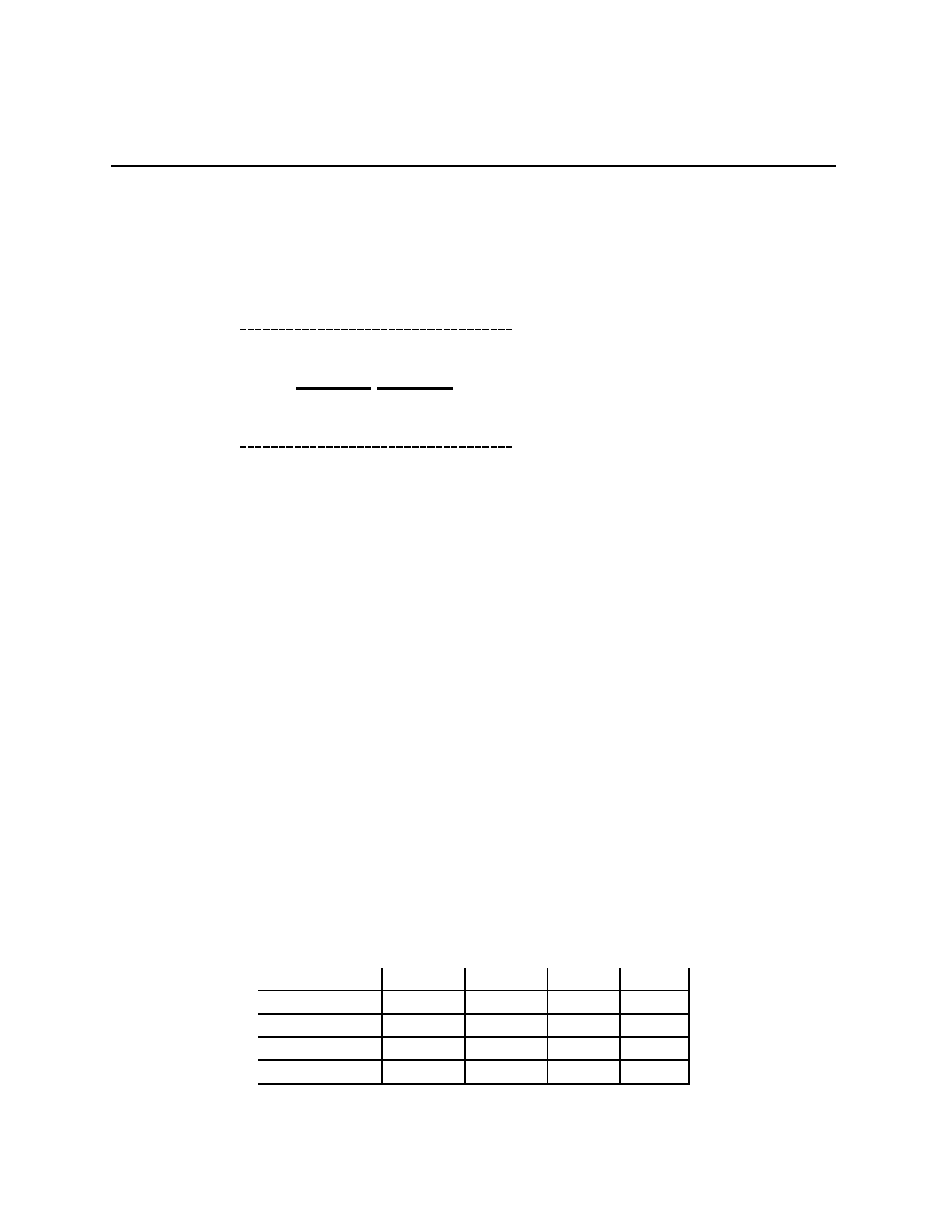
Chapter 4.6

strong

weak

0.9

0.1

beer

quiche

Bully

−10

There is a fellow who, on 9 out of every 10 days on average, rolls out of bed like Popeye

on spinach. When he does this we call him “strong.” When strong, this fellow likes nothing
better than Beer for breakfast. On the other days he rolls out of bed like a graduate student
recovering from a comprehensive exam. When he does this we call him “weak.” When weak,
this fellow likes nothing better than Quiche for breakfast. In the town where this schizoid
personality lives, there is also a swaggering bully. Swaggering bullies are cowards who, as a
result of deep childhood traumas, need to impress their peers by picking on others. Being
a coward, he would rather pick on someone weak. He makes his decision about whether to
pick, p, or not, n, after having observed what the schizoid had for breakfast.

We are going to solve this game in two different fashions, the first works with the

normal form, the second uses what is called the agent normal form. The agent normal form
corresponds to a different version of the motivating story above, and solving it by iterated
deletion requires the use of self-referential tests.

Working in the normal form

Taking expectations over Nature’s move, the 4

× 4 normal form for this game is

(st,wk)

\(b,q)

(p, p)

(p, n)

(n, p)

(n, n)

(b, b)

(9,

−8)

(9,

−8)

(29, 0)

(b, q)

(10,

−8) (12, −9) (28, 1) (30, 0)

(q, b)

(0,

−8)

(18, 1)

(2,

−8) (20, 0)

(q, q)

(1,

−8)

(21, 0)

(1,

−8) (21, 0)

101

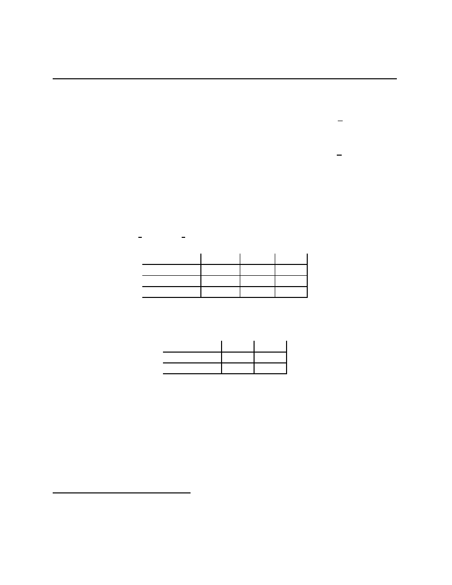
Chapter 4.6

The equilibrium set for this game can be partitioned into E

and E

where

{((q, q), (0, β, 0, 1 − β)) : 21 ≥ 12β + 30(1 − β), i.e. β ≥

and

{((b, b), (0, 0, β, 1 − β)) : 29 ≥ 28β + 30(1 − β) i.e. β ≥

Note that

O(·) is constant on the two closed and connected sets E

and E

, so that once

again, the players are indifferent to points within the sets E

. The quiche-eating set of

equilibria, E

, is not intuitive. Any σ

∈ E

corresponds to the weak type hiding behind

the shadow of the strong type, but the strong type not getting what they want. Iterated
deletion of weakly dominated strategies kills all of E

and all but one point in E

The strategy (p, p) is strictly dominated by (n, n) for the bully, the strategy (q, b) is

strictly dominated by

on (b, q),

on (q, q). Eliminating these gives the game

(st,wk)

\(b,q)

(p, n)

(n, p)

(n, n)

(b, b)

(9,

−8)

(29, 0)

(b, q)

(12,

−9) (28, 1) (30, 0)

(q, q)

(21, 0)

(1,

−8) (21, 0)

In this game, (n, n) weakly dominates (p, n) for 2, and once (p, n) is eliminated, (b, b)

and (b, q) strongly dominated (q, q) for 1. Eliminating these gives the game

(st,wk)

\(b,q) (n, p)

(n, n)

(b, b)

(29, 0)

(b, q)

(28, 1)

(30, 0)

In this game, (n, p) weakly dominates (n, n), once (n, n) is removed, (b, b) is 1’s strict best

response, so the only equilibrium to survive iterated deletion of weakly dominated strategies
is ((b, b), (n, p)), i.e. both types have Beer for breakfast and the Bully leaves anyone having
Beer alone, but picks a fight with anyone having Quiche for breakfast.

Working in the agent normal form

Consider the following, rather different version of the same basic story: 9 out of every 10

days on average, a stranger who feels like Glint Westwood

comes into town. We call such

A mythical Hollywood quasi-hero, who, by strength, trickiness and vile cigars, single-handedly over-

comes huge obstacles, up to and including bands of 20 heavily armed professional killers.

102

Chapter 4.6

strangers “strong.” Strong strangers like nothing better than Beer (and a vile cigar) for
breakfast. On the other days, a different kind of stranger comes to town, one who feels like
a graduate student recovering from a comprehensive exam. We call such strangers “weak.”
Weak strangers like nothing better than Quiche for breakfast. Strong and weak strangers are
not distinguishable to anyone but themselves. In the town frequented by breakfast-eating
strangers, there is also a swaggering bully. Swaggering bullies are cowards who, as a result of
deep childhood traumas, need to impress their peers by picking on others. Being a coward,
he would rather pick on someone weak. He makes his decision about whether to pick, p, or
not, n, after having observed what the stranger had for breakfast. With payoffs listed in
the order 1

, 1

, 2 and normalizing strangers’ payoffs to 0 when they are not breakfasting

in this town, the game tree is

strong

weak

0.9

0.1

beer

quiche

Bully

−10

This game has three players (four if you include Nature), 1

(aka Glint), 1

(aka the

weak stranger), and 2 (aka the Bully). In principle, we could also split the Bully into two
different people depending on whether or not they observed Beer or Quiche being eaten.
The logic is that we are the sum of our experiences, and if our experiences are different, then
we are different people. If we did this second agent splitting, we would have the game in
what is called agent normal form. In this game, instead of putting 0’s as the utilities for
the strangers’ when they are not breakfasting in this town, we could have made 1

’s utility

equal to 1

’s even when they are out of town. Since we are changing utilities by adding

a function that depends only on what someone else is doing, this cannot change anything
about the equilibrium set.

103

Chapter 4.6

More generally, to give the agent normal form for an extensive form game, 1) for each

∈ U

∈ P

(go back and look at the notation for extensive form games if you have already

forgotten it), we invent a new agent i

, 2) we assign all “copies” of each i the same utility at

each terminal node. This is a bit confusing — we are acting as if these are different people,
but they are different people with exactly the same preferences. There are two reasons for
this confusing choice:

1. It leads to Kuhn’s theorem, an extremely important result that we will get to in a

while.

2. We would like the sets of equilibrium outcomes to be the same in the original game and

in the agent normal form version of the game. In the signaling game above, since no
players’ information sets ever precede each other, the different copies having different
utilities didn’t matter. It would matter if 1

made a choice that impacted 1

’s utility

and subsequent choices.

2 still has a dominated strategy, (p, p). By varying 2’s strategy amongst the remaining

3, we can make either Beer or Quiche be a strict best response for both strangers. This
means that no strategies are dominated for the strangers, and iterated deletion of dominated
strategies stops after one round.

Again, the equilibrium set for this game can be partitioned into two sets, E

and E

but note that we must now specify 3 strategies,

{((q), (q), (0, β, 0, 1 − β)) : 21 ≥ 12β + 30(1 − β), i.e. β ≥

and

{((b), (b), (0, 0, β, 1 − β)) : 29 ≥ 28β + 30(1 − β) i.e. β ≥

1
2

Again,

O(·) is constant on the two closed and connected sets E

and E

However, the self-referential tests do eliminate E

— for 1

, Beer is dominated relative

to E

, after removing Beer for 1

, (p, n) is weakly dominated for 2, implying that no σ

∈ E

survives the iterative steps. It is fairly easy to check (and you should do it) that E

does

survive the iterative steps of the self-referential tests.

Morals about the difference between a game and its agent normal form

First, whether or not we should use a particular game, its agent normal form, or some

hybrid (as above where we did not split player 2) depends on what story we are telling.
Games boil away a great deal of contextual detail, this is the source of their power as story-
telling devices. Trying to make a blanket pronouncement about which form is generally

104

Chapter 4.7

correct is like trying to decide, on the basis of the game matrix, which of the Partners
(in the Battle of the Partners coordination game) is dominant in the sphere of week-end
entertainment. This is a ridiculous exercise, both because any answer must be intellectually
bankrupt, and because any answer would lessen our ability to explain.

Second, even though the set of equilibrium outcomes is the same in a game and in the

agent normal form of the game, splitting agents makes a huge difference to the power of
iterated deletion arguments, even in games where the copies of an agent do not play after
each other.

4.7

Kuhn’s Theorem

In the normal form of the Beer-Quiche game, there were 4 pure strategies, implying that the
set of mixed strategies is 3-dimensional. When we looked at the agent normal form, the two
versions of player 1, 1

and 1

, had 1-dimensional sets of mixed strategies. If we can show

that every one of the 3-dimensional mixed strategies can be replicated by stochastically
independent choices by 1

and 1

, then we can save one dimension in our analysis of the

equilibria. The content of Kuhn’s theorem is that we can replicate any mixed strategy by
use of stochastically independent choices made in the agent normal form of the game.

Saving one dimension may not seem like much, there are other games in which the

savings are immense.

Problem 4.24 Let Γ be a 2

× 2 game. Play Γ repeatedly, say for n times, and at the end

of each play of the game, suppose that each player observes the complete previous play of
the game.

1. Draw a game tree to represent this situation for n = 2.

2. As a function of n, give the number of pure strategies for player i.

3. Again as a function of n, give the dimensionality of the space of strategies in the agent

normal form.

A behavior strategy for i, b

, is a mapping from i’s information sets, the H

∈ U

a partition of P

, to distributions over the actions available at the information set. The

probabilities, b

(

·|U

) and b

(

·|U

), U

6= U

, are interpreted as stochastically independent.

This is just as if agents at all information sets were different. One way to understand
behavioral strategies is that they are “local” randomizations, local to the information set. A
mixed strategies is a global randomization, a once and for all randomization over contingent
plans.

105

Chapter 4.7

It is clear that any behavioral strategy specifies a distribution over pure strategies. To

talk of replacing mixed strategies by equivalent behavioral strategies, we must say what it
means for strategies to be equivalent. Two mixed strategies σ

and σ

are equivalent in an

extensive form game if for all σ

∈ A and for decision nodes x, O(σ\σ

|x) = O(σ\σ

|x).

Problem 4.25 In the following game, verify that for every mixed strategy σ

for player,

there is a behavioral strategy, b

, with the property that for all σ and all non-terminal nodes

O(σ\σ

|x) = O(σ\b

|x).

•

)

Fix a mixed strategy σ

for i. We are going to use σ

to generate a behavioral strategy

that is equivalent to σ

. For H

∈ U

, let

(H) =

∈ A

: (

∃s

∈ A)[O(s

\s)(Z(H)) > 0] }

where Z(H) is the set of terminal nodes that follow H. In words, R

(H) is the set of i’s

strategies that do not absolutely preclude reaching H. If σ

(H)) > 0, define

|H) =

(H)

∩ {a

: s

(H) = a

})

(H))

that is, b

|H) is the probability that a

is chosen by i given that some pure strategy

106

Chapter 4.8

possibly reaching H is played. If σ

(H)) = 0, that is, σ

precludes reaching H, define

|H) = σ

(

: s

(H) = a

}),

that is, b

|H) is the probability that a

is chosen by i at H without conditioning on having

reached H.

Go through a couple of examples to show that the mapping from mixed strategies to

behavioral strategies can be many-to-one, and to show that mixed strategies are equivalent
to the behavioral strategies given above.

Theorem 4.5 (Kuhn) Every mixed strategy σ

is equivalent to its generated b

, and each

is equivalent to any of the σ

that generate it.

4.8

Equivalence of games

There are innocuous transformations of games that should not affect our analysis of equilib-
ria. The easiest of these involves clumping duplicate strategies together as one strategy. Two
strategies are duplicates if no-one cares about the difference between the two. Formally,

Definition 4.6 In a game Γ = (A

, u

)

i∈I

, t

and t

are duplicates if

(

∀j ∈ I)(∀s ∈ A)[u

) = u

)].

Remember that in extensive form games, u

(s) = u

(

O(s)), and duplicates work through

the outcome function.

Consider the following version of the money-burning game.

Out

Player 1’s pure strategies are A

{(Out, L), (Out, R), (In, L), (In, R)}. The 4 × 2

normal form for this game is

107

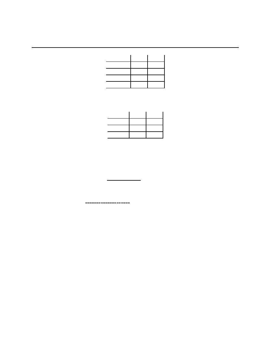
Chapter 4.8

(Out, L)

(2, 9)

(Out, R)

(2, 9)

(In, L)

(5, 1)

(0, 0)

(In, R)

(0, 0)

(1, 5)

It is pretty clear that (Out, L) and (Out, R) are duplicates. Let us give them one name,

say Out. This gives the The 3

× 2 normal form for this game is

(Out)

(2, 9)

(In, L)

(5, 1)

(0, 0)

(In, R)

(0, 0)

(1, 5)

The normal form that results from an extensive form game after duplicate strategies

have been identified is called the semi-reduced norm form, so the 3

× 2 game is the

semi-reduced normal form for the money burning game given above. It corresponds directly
to the following (and other) extensive form games

Out

The following contains a list of transformations of a game. Game theorists generally

agree that these transformations do not change the structure of a semi-reduced normal form
game, at least not too much. Notice that the list does not include splitting up an agent
as we do when we look at the agent normal form of a game. We have seen that iterated
deletion arguments have very different implications after such changes.

Theorem 4.7 Γ and Γ

have the same semi-reduced normal form if we can reach Γ

from

Γ by applying a finite sequence of the following transformations or their inverses (given in
parantheses).

1. Identifying (adding) duplicate strategies.

108

Chapter 4.9

2. Expanding (coalescing) a choice: Partition the action set A(H) at H into A and A,

have the agent first choose between A and A, and choose between the actions in A and
the actions in A.

3. Interchanging (interchanging) simultaneous moves.

4. Integrating out (adding moves by) Nature: If a chance move leads only to terminal

nodes, replace this move and its terminal successors by a single terminal node with the
corresponding expected payoffs.

5. Addition (subtraction) of a superfluous decision point: Let H be an information set

at which i moves, z

6∈ Z(H) a terminal node. If y precedes z, add a decision point

∈ H immediately before y such that after x, any action in A(H) leads to a copy of

y and such that no j

6= i gets to hear which choice was taken at x.

The reduced normal form of a game reverses all of the agent splitting that goes into

making the agent normal form of a game. Go back to Problems 4.10. From it you can
conclude that a solution concept for games that satisfies existence, invariance (a solution to
a game is a solution to any game having the same reduced normal form), undominatedness
(no player puts positive mass on a weakly dominated strategy), and iterated dominance (a
solution to a game contains a solution of any game obtained by the deletion of a strategy
which is dominated against the set), must violate the backward induction axiom, which
states that

For any extensive form game, a solution of the normal form of that game contains
a solution of the agent normal form of the game.

So, we have seen, several times now, that agent splitting, while being innocuous for the

set of Nash equilibria, and even making it relatively easy (by Kuhn’s theorem) to find the
Nash equilibria, has very strong effects on the various subsets of equilibria that we study.

4.9

Some other problems

Your homework is any three of the following seven problems. I’d recommend that you look
at all of them well enough to know how to set them up.

Problem 4.26 In the spying and coordination game, fully analyze the equilibrium sets of
both games. [This means give the normal form, the agent normal form, the sets of Nash
equilibria on which the outcome function is constant, the equilibria that survive iterated dele-
tion of weakly dominated strategies, and the equilibrium sets that survive the self-referential
tests.]

109

Chapter 4.9

Problem 4.27 In the going to war as a signal games, fully analyze the equilibrium sets. In
particular, in comparing the two games with and without sleepers, evaluate the statement,
“When spying is cheap, it lowers the probability of war.”

Problem 4.28 In the “same structure, less story” game, fully analyze the equilibrium set
as a function of x.

Problem 4.29 A seller values an object at 0 and would like to sell to a potential buyer with
a valuation that takes the value a > 0 with probability ρ, 0 < ρ < 1, and takes the value
b > a with probability 1

− ρ. Thus, for either of the potential buyer’s valuations, there is

the possibility of mutually improving trade. The seller chooses a “take-it-or-leave-it” price,
p

∈ [0, ∞), and the buyer responds by accepting or rejecting the offer, ending the game.

1. Characterize the pure strategy Nash equilibria of this game.

2. Characterize the pure strategy subgame perfect equilibria of this game.

3. When are the subgame perfect equilibria of this game inefficient?

4. Suppose that the game is changed so that, if the first offer is rejected, the buyer has

the option to make a second offer, but that this offer will be the last. Supposing that
payoffs are not discounted, evaluate the efficiency of the subgame perfect equilibria of
this game.

Problem 4.30 Consider a market with one incumbent firm and a potential entrant. The
potential entrant has low costs with probability 0.2, and has high costs with probability 0.8.
The actual costs (low or high) of the entrant are private information to the entrant, who
decides whether to stay “out” or “enter.” The outside option for the low cost entrant has an
expected utility of 25, while the outside option for the high cost entrant has an expected utility
of 0. If the potential entrant stays out, then the incumbent has an expected utility of 25. If the
potential entrant enters, then the incumbent decides whether to “fight” or “acquiesce.” If the
incumbent fights, then the payoffs for the entrant and incumbent respectively are (20,

−25)

when the entrant is low cost, and (

−10, 40) when the entrant is high cost. If the incumbent

acquiesces, then the payoffs are (40, 10) when the entrant is low cost, and (20, 30) when the
entrant is high cost.

1. Give the extensive and normal forms for this game.

2. Partition the set of equilibria into closed and connected sets on which the outcome

functions is constant.

110

Chapter 4.9

3. Which of the closed and connected sets that you found survive iterated deletion of

weakly dominated strategies. Which survive the self-referential test?

4. Do your answers to the previous question change if you work in the agent normal

form?

Problem 4.31 (Spence labor market model) An employer faces two types of employ-
ees, types t = 1, 3. An employee of type t produces t, that is, type has been identified with
marginal product. The proportion of t = 1 employees is q

∈ (0, 1), and the proportion of

t = 3 employees is 1

− q. The employer cannot observe a potential employee’s type, but can

observe the educational level obtained before the hiring decision occurs. Type t employees
incur a utility cost of E(9

− 3t)/2 to acquire education level E.

1. Formulate this situation as a signaling game.

2. Give the pooling equilibrium or equilibria of the signaling game.

3. Give the separating equilibrium or equilibria.

4. Show that the self-referential tests may pick between the pooling and the separating

cases.

Problem 4.32 Fully analyze the equilibrium of Felicia game with the self-referential tech-
niques.

111

Chapter 4.9

112

Chapter 5

Mathematics for Game Theory

We’ll begin with a review of “real” numbers, trying to understand them as a special (very
special) metric space built up from the rational numbers. This requires sequences, which
we will also use to talk about limits, closure, continuity, and compactness. We will prove
one fixed point theorem, the one known as the contraction mapping theorem, and we will
discuss another one, Kakutani’s fixed point theorem. This last one was designed for game
theory, and directly implies the existence of Nash equilibria. With one additional step, it
implies the existence of Hillas stable sets of equilibria. These are closed, connected sets
of equilibria that survive self-referential tests. Hillas stable sets are always a subset of the
perfect equilibria and always contain a proper equilibrium, and these two solution concepts
will be treated with the tools developed here.

5.1

Rational numbers, sequences, real numbers

Intuitions about integers, denoted

N, are very strong, they have to do with counting things.

Including 0 and the negative integers gives us

Z. The rationals, Q, are the ratios m/n,

m, n

∈ Z, n 6= 0. We can do all physical measurements using Q because they have a

denseness property — if q, q

∈ Q, q 6= q

, then there exists a q

strictly between q and q

(One visual image, if we were to imagine stretching the rational numbers out one after the
other, nothing of any width whatever could get through.)

One of the theoretical problems with

Q as a model of quantities is that there are easy

geometric constructions that yield lengths that do not belong to

Q — consider the length of

the diagonal of a unit square, by Pythagoras’ Theorem, this length is

√

2, if

√

2 = m/n for

some m, n

∈ N, n 6= 0, then by cancellation, we know that at most one of the integers m and

n are even, however, cross multiplying and then squaring both sides of the equality gives
2n

= m

, so it must have been m that is even, but if m is even, it is of the form 2m

and

= 4(m

)

giving 2n

= 4(m

)

which is equivalent to n

= 2(m

)

, which implies that n

113

Chapter 5.1

is even, (

⇒⇐). If you believe that all geometric lengths must exist, i.e. you believe in some

kind of deep connection between numbers that we can imagine and physical measurements,
this observation could upset you, and it might make you want to add some new “numbers”
to

Q, at the very least to make geometry easier. The easiest way to add these new numbers

is an example of a process called completing a metric space. It requires some preparation.

A sequence in a set X is a mapping from

N to X. A sequence q

Q is a Cauchy

sequence if

(

∀q > 0, q ∈ Q)(∃M ∈ N)(∀n, n

≥ M)[|x

− x

| < q].

The set of all Cauchy sequences in

C. We say that two Cauchy sequences, x

, y

, in

Q are

equivalent if

(

∀q > 0, q ∈ Q)(∃N ∈ N)(∀n ≥ M)[|x

− y

| < q].

The set of real numbers,

R, is, by definition, the set of equivalence classes of Cauchy se-

quences. For any Cauchy sequence x

, [x

] denotes the Cauchy equivalence class. For

example,

√

2 = [1, 1.4, 1.41, 1.414, 1.4142, 1.41421, 1.414213, . . .].

Notice that

√

2 = [1.5, 1.45, 1.415, 1.4145, 1.41425, 1.414215, 1.4142135, . . .]

because this second sequence is equivalent to the first one. The constant sequences are
important, for any q

∈ Q, we’ll use the symbol “q” to mean the equivalence class of the

constant sequence,

q = [q, q, q, . . .].

Looking at the constant sequences shows that we have imbedded

Q in R.

We understood addition, subtraction, multiplication, and division for

Q, we just extend

our understanding in a fashion very close to the limit construction. Specifically,

] + [y

] = [x

+ y

], [x

]

· [y

] = [x

· y

], [x

]/[y

] = [x

], [x

]

− [y

] = [x

− y

While these definitions seem immediately correct, to be thorough we must check that if x

and y

are Cauchy, then the sequences x

+ y

, x

· y

, x

, and x

− y

are also Cauchy.

So long as we avoid division by 0, they are.

Problem 5.1 Show that if x

and y

are Cauchy sequences in

Q, then the sequences x

and x

· y

are also Cauchy.

The last problem doesn’t quite finish the job of transfering our understandings of addi-

tion, subtraction, multiplication, and division to

R. What’s missing is the statement that

all sequences in any equivalence classe is treated the same way.

114

Chapter 5.2

Problem 5.2 Suppose that x

and y

are Cauchy sequences. If r

is equivalent to x

and

is equivalent to y

, then r

+ s

is equivalent to x

+ y

and r

· s

is equivalent to x

· y

If a function f :

Q → Q has the property that f(x

) is a Cauchy sequence whenever

is a Cauchy sequence, then f (

·) can be extended to a function f : R → R by defining

f ([x

]) = [f (x

)]. For example, Problem 5.1 implies that any polynomial P (

·) with rational

coefficients can be extended in this fashion. Letting the rational coefficients converge to real
coefficients completes the rest of the story for polynomials.

Now it is time to extend the concepts of “greater than” and “less than” from

Q to R. We

say that a number r = [x

]

∈ R is greater than 0 (or strictly positive) if there exists a q ∈ Q,

q > 0, such that (

∃N ∈ N)(∀n ≥ N)[q ≤ x

]. We say that [x

] > [y

] if [x

]

− [y

] is strictly

positive. The set of strictly real numbers is denoted

. Note that if [x

] > [y

], then it

is not the case that [y

] > [x

]. Further, if it not the case that [x

] > [y

] or [y

] > [x

then [x

] = [y

], that is, the sequence x

and y

are (Cauchy-)equivalent. The notational

version of this is [x

]

≥ [y

] if [x

] > [y

] or [x

] = [y

Now that we know what “>” and “

≥” mean, define

max

{x, y} =

if x

≥ y

if y

≥ x

From this, we can define

|x| = max{x, −x}. In turn, this leads to defining the distance

between x and y in

R by d(x, y) = |x − y|. The function d : R × R → R

is called a metric.

There are many metrics on many sets. We introduce the abstraction based d(

·, ·) on the R,

the idea of a metric space. A metric space is a pair (X, d) where X

6= ∅, d : X × X → R

where d(

·, ·) satisfies three conditions:

1. (symmetry) (

∀x, y ∈ X)[d(x, y) = d(y, x)],

2. (distinguishes points) d(x, y) = 0 if and only if x = y,

3. (triangle law) (

∀x, y, z ∈ X)[d(x, y) + d(y, z) ≥ d(x, z)].

Examples: X =

N with d(x, y) = |x − y|; X = Q with d(x, y) = |x − y|; X = R

with

d(x, y) = [

n
i=1

− y

]

1/p

, p

≥ 1 (here we could work by defining kxk

= [

n
i=1

]

1/p

and d(x, y) =

kx − yk

); X = C[0, 1] with d(x, y) = max

t∈[0,1]

|x(t) − y(t)|; [−B, +B]

for

any (non-empty) set S with d(x, y) = sup

s∈S

|x(s) − y(s)|.

The last pair of examples are quite important, and use results that we do not yet have.

One is that we need to show that max

t∈[0,1]

|x(t) − y(t)| exits when x, y are continuous

functions (and one of the reasons we don’t have it is because we haven’t defined continuous
functions). The other is that we haven’t said what “sup” is. It’s also known as a “least
upper bound,” or lub.

115

Chapter 5.2

5.2

Limits, completeness, glb’s and lub’s

We’ll begin with limits, then discuss completeness, glb’s and lub’s, and then turn to the
contraction mapping theorem. The contraction mapping theorem will lead us on a detour
through stationary Markov chains and discounted dynamic programming.

5.2.1

Limits

A sequence x

in a metric space (X, d) has a limit x if

(

∀ ∈ R

)(

∃N ∈ N)(∀n ≥ N)[d(x

, x) < ].

This is written as x

→ x which is said as “x

converges to x.”

Problem 5.3 Using only what has been given above, show that in the metric space (

R, d),

d(x, y) =

|x − y|, the sequence x

= 2

−n

converges to x = 0.

A sequence r

R is Cauchy if

(

∀ ∈ R

)(

∃M ∈ N)(∀n, n

≥ M)[|r

− r

| < ].

Theorem 5.1 If r

is a Cauchy sequence in

R if and only if there exists an r ∈ R such

that r

→ r.

The property that Cauchy sequences converge is very important. There are a huge

number of inductive constructions of an x

that we can show is Cauchy. Knowing there

is a limit in this context gives a good short-hand name for the result of the inductive
construction. Some examples: the irrational numbers that help us do geometry; Brownian
motion that helps us understand finance markets; value functions that help us do dynamic
programming both in micro and in macro. Only the first of these examples happens in

it is time to generalize the property that Cauchy sequences converge.

5.2.2

Completeness

A sequence in a metric space (X, d) is Cauchy if

(

∀ ∈ R

)(

∃M ∈ N)(∀n, n

≥ M)[|x

− x

| < ].

The set of all Cauchy sequences in X is

C(X). Two Cauchy sequences, x

, y

, in X are

equivalent if

d(x

, y

)

→ 0 in R.

116

Chapter 5.2

The set of equivalence classes of Cauchy sequences is called the completion of X and is
denoted b

X. For example,

R = b

Q. Let x = [x

], y = [y

], we can define b

d(x, y) as the limit

of the sequence d(x

, y

) (though this takes proving that the limit exists, this however, is a

consequence of the sequence d(x

, y

) being Cauchy and Theorem 5.1).

A metric space (X, d) is called complete if every Cauchy in X converges to some point

in X. Theorem 5.1 is just the statement that

R is complete with the usual metric. This is

just a special case of

Theorem 5.2 For any metric space (X, d), ( b

X, b

d) is complete.

Problem 5.4 Prove this theorem.

5.2.3

Greatest lower bounds and least upper bounds

Some subsets of

R do not have minima, even if they are bounded, e.g. S = (0, 1]. The

concept of a greatest lower bound, also known as an infimum, fills this gap.

Some subsets of

R do not have maxima, even if they are bounded, e.g. S = [0, 1). The

concept of a least upper bound, also known as a supremum, fills this gap.

Which one works with, infima or suprema, is a matter of taste. In reading the following

discussion of infima, be sure to go through what would change if we were discussing suprema.

A set S

⊂ R is bounded below if there exists an r ∈ R such that for all s ∈ S, r ≤ S.

This is written as r

≤ S. A number s is a greatest lower bound (glb) for or infimum

of S if s is a lower bound and s

> s implies that s

is not a lower bound for S. Equivalently,

that s is a glb for S if s

≤ S and for all > 0, there exists an s ∈ S such that s < s + . If

it exists, the glb of S is often written inf S.

Problem 5.5 If s and s

are glb’s for S

⊂ R, then s = s

. In other words, the glb, if it

exists, is unique.

Theorem 5.3 If S

⊂ R is bounded below, there there exists an s ∈ R such that s is the glb

for S.

Proof: Let r be any lower bound for S, set r

= r, given that r

has been defined, define

n+1

to be r

+ 2

m(n)

with m(n) = max

{m ∈ Z : r

+ 2

≤ S} using the conventions that

max

∅ = −∞ and 2

−∞

= 0. By construction, the sequence r

is weakly increasing, and is a

Cauchy sequence. Let s = lim

(which exists because

R is complete).

The proof will be finished when we show that s is the infimum. For this we must show

that s

≤ S and if s

> s, then

∃x ∈ S such that x < s

1. If it is not the case that s

≤ S, then there exists x ∈ S such that x < s. Since

→ s, for sufficiently large n, r

> x (by convergence of r

to s). This contradicts

the definition of r

. Therefore s is a lower bound for S.

117

Chapter 5.3

2. Pick arbitrary s

> s and suppose that (s, s

)

∩ S = ∅. Let δ = s

− s > 0. Pick m

to be the largest m such that 2

< δ. Pick N such that for all n

≥ N, r

> s

− 2

Then r

N +1

≥ r

+ 2

> s. Since the sequence is weakly increasing, this contradicts

→ s.

An alternative development of

R starts with Q and adds enough points to Q so that the

resulting set satisfies the property that all sets bounded below have a greatest lower bound.
Though more popular as an axiomatic treatment, I find the present development to be both
more intuitive and more broadly useful, as well as being an instructive parallel when it
comes time to develop other models of quantities. I wouldn’t overstate the advantage too
much though, there are very good axiomatic developments of the other models of quantities.

Before turning to contraction mappings, let us go back to the space X = [

−B, +B]

for

any (non-empty) set S with d(x, y) = sup

s∈S

|x(s) − y(s)|.

Lemma 5.4 When X = [

−B, +B]

and d(x, y) = sup

s∈S

|x(s) − y(s)|, (X, d) is a complete

metric space.

This will be useful when S is the set of states for a dynamic programming problem

and we are interested in bounded value functions, that is, functions that map from S to
[

−B, +B].

5.3

The contraction mapping theorem and applications

Let (X, d) be a metric space. A mapping f from X to X is a contraction mapping if

(

∃β ∈ (0, 1) )(∀x, y ∈ X)[d(f(x), f(y)) < βd(x, y)].

Lemma 5.5 If f : X

→ X is a contraction mapping, then for all x ∈ X, the sequence

x, f

(1)

(x) = f (x), f

(2)

(x) = f (f

(1)

(x)), . . . , f

(n)

(x) = f (f

(n−1)

(x)), . . .

is a Cauchy sequence.

Problem 5.6 Prove the lemma.

A fixed point of a mapping f : X

→ X is a point x

∗

such that f (x

∗

) = x

∗

. Note

that when X =

, f (x

∗

) = x

∗

if and only if g(x

∗

) = 0 where g(x) = f (x)

− x. Thus, fixed

point existence theorems may tell about the solutions to systems of equations.

118

Chapter 5.3

Theorem 5.6 (Contraction mapping) If f : X

→ X is a contraction mapping and

(X, d) is a complete metric space, then there exists a unique x

∗

such that f (x

∗

) = x

∗

, and

for all x

∈ X, the sequence

x, f

(1)

(x) = f (x), f

(2)

(x) = f (f

(1)

(x)), . . . , f

(n)

(x) = f (f

(n−1)

(x)), . . .

converges to x

∗

Proof: Let x

(x) = f

(n)

(x). From the previous Lemma, we know that

∀x, x

(x) is Cauchy.

Pick an arbitrary x, x

∈ X. Since X is complete, x

(x)

→ x

∗

for some x

∗

. Since f is a

contraction mapping,

d(x

(x), x

))

≤ βd(x, x

d(x

(x), x

))

≤ βd(x

(x), x

))

≤ β

d(x, x

≤

. ,

d(x

(x), x

))

≤ β

d(x, x

≤

Since 0 < β < 1, β

→ 0. Thus, x

(x) is Cauchy, and d(x

(x), x

))

→ 0 so that x

)

is Cauchy equivalent to x

(x). These imply that x

(x) and x

) both converge to x

∗

To show that f (x

∗

) = x

∗

, we’ll pick an arbitrary > 0 and show that d(x

∗

, f (x

∗

)) < .

So, pick arbitrary > 0. For some x

∈ X, let x

= f

(n)

(x) so that x

→ x

∗

. By the triangle

inequality,

d(x

∗

, f (x

∗

))

≤ d(x

∗

, x

) + d(x

, x

n+1

) + d(x

n+1

, f (x

∗

)).

Because f is a contraction mapping, the last term, d(x

n+1

, f (x

∗

)), is less than or equal to

βd(x

, x

∗

). Now pick M such that for all n, m

≥ M, d(x

∗

, x

) < /3 and d(x

, x

) < /3.

Combining,

d(x

∗

, f (x

∗

))

≤ d(x

∗

, x

) + d(x

, x

n+1

) + d(x

n+1

, f (x

∗

)) < /3 + /3 + β/3 < ,

which completes the proof.

5.3.1

Stationary Markov chains

For our purposes, a stochastic process is a sequence (X

)

∞

t=0

of random variables taking

values in a finite space S. Stationary Markov chains are a special kind of stochastic process.

Let P

be a distribution on S. A stationary Markov chain is a stochastic process

with the property that P

is the distribution of X

, and there is a matrix P = (P

i,j

)

i,j∈S

119

Chapter 5.3

such that

(

∀t)[P (X

t+1

= j

= i

, . . . , X

t−1

= i

t−1

, X

= i) = P (X

t+1

= j

= i) = P

i,j

In particular, this requires that

(

∀i)[

j∈S

i,j

= 1].

The matrix P is called the one-step transition matrix. This name comes from the

following observation: if π

is the (row) vector of probabilities describing the distribution

of X

, then π

P is the (row) vector describing the distribution of X

t+1

. This means that

7→ πP is a mapping from ∆(S) to ∆(S). If this mapping is a contraction, we can apply

the contraction mapping theorem, because, as we will see, ∆(S) is complete.

It seems that Markov chains must have small memories, after all, the distribution of

t+1

depends only on the state at time t. This can be “fixed” by expanding the state space,

e.g. replace S with S

× S and the last two realizations of the original X

can influence

what happens next. To be specific here, we want P (X

t+1

= j

= i

, X

t−1

= i

t−1

). Let

= [X

, X

t−1

] and Y

t+1

= [X

t+1

, X

], so that P (Y

t+1

= [j, j

]

= i

, X

t−1

= i

t−1

) should

be a Markov matrix subject to the restriction that it can only be positive if j

= i

. An

expanded version of the same device works if we want k-period histories to determine the
transition probabilities from t to t + 1.

For i, j

∈ S, let P

(n)

i,j

= P (X

t+n

= j

= i). The matrix P

(n)

is called the n-step

transition matrix. One of the basic rules for stationary Markov chains is called the
Chapman-Kolmogorov equation,

(

∀1 < m < n)

(n)

i,j

k∈S

(m)

· P

(n−m)

This means that if π

is the (row) vector of probabilities describing the distribution of

, then π

(n)

is the (row) vector describing the distribution of X

t+n

. Further, the matrix

(n)

is really P

, the matrix P multiplied by itself n times.

Let ∆(S) denote the set of probabilities on S. π

∈ ∆(S) is an ergodic distribution

for P if π

P = π

Problem 5.7 Solve for the set of ergodic distributions for each of the following P where
α, β

∈ (0, 1):

1 0
0 1

0 1
1 0

− α)

− β)

− β) β

120

Chapter 5.3

Theorem 5.7 If S is finite and P

0, then the mapping π

7→ π

P from ∆(S) to ∆(S)

is a contraction mapping.

Proof: For each j

∈ S, let m

= min

i,j

. Because P

0, we know that for all j, m

> 0.

Define m =

. We will show that for p, q

∈ ∆(S), kpP − qP k

≤ (1 − m)kp − qk

kpP − qP k

j∈S

i∈S

− q

i,j

j∈S

i∈S

− q

)(P

i,j

− m

) +

i∈S

− q

≤

j∈S

i∈S

− q

|(P

i,j

− m

) +

j∈S

i∈S

− q

)

i∈S

− q

j∈S

i,j

− m

) + 0

kp − qk

· (1 − m)

where the next-to-last equality follows from the observation that p, q

∈ ∆(S), and the last

equality follows from the observation that for all i

∈ S,

j∈S

i,j

= 1 and

j∈S

= m.

Provided that ∆(S) is complete (it is, we just haven’t proven it yet), Theorem 5.7 gives

a sufficient condition for πP

→ q

∗

where q

∗

is unique. The condition is sufficient, but it is

not necessary. Consider the matrix

P =

− β) β

Note that (1, 0)P

= (1, 0), (0, 1)P

= ((1

−β

), β

), so that for all a

∈ [0, 1], (a, 1−a)P

a(1, 0) + (1

− a)((1 − β

), β

)

→ (1, 0).

Another instructive example is the matrix

P =





 .

Even though P has some 0 entries, P

0. Theorem 5.7 tells us that for every π, πP

→

∗

. Further, πP

2n+1

= (πP )P

→ q

∗

, so that the entire sequence πP

→ q

∗

. Generalizing

this observation proves

Corollary 5.8 If there exists N such that P

0, then there exists a unique q

∗

such that

121

Chapter 5.3

for all π, πP

→ q

∗

If P has the property that there exists a unique q

∗

such that for all π, πP

→ q

∗

, then

we say that P is a stationary ergodic Markov chain. This is the best kind of Markov
chain to analyze.

About ∆(S) being a complete metric space: Let p

be a Cauchy sequence in ∆(S)

⊂ R

;

Since

is complete, p

→ x for some x ∈ R

; What we need to show is that x

∈ ∆(S);

Show that x

≥ 0; Show that

x(s) = 1.

Problem 5.8 Under the conditions of Theorem 5.7, show that the matrix P

converges

and characterize the limit. [With e

being the unit vector in the i’th direction, note that

→ q

∗

where q

∗

is the unique ergodic distribution.]

By the way, there are mappings f such that f

is a contraction mapping but f is not.

Example 5.9 Let X =

, d(x, y) =

|x − y|, and let f be the cdf of the uniform dis-

tribution on the interval (1, 2). For x, y

∈ (1, 2), d(f(x), f(y)) = d(x, y), but for all x, y,

d(f

(x), f

(y)) = 0.

5.3.2

Some evolutionary arguments about equilibria

Fix a finite game Γ = (A

, u

)

i∈I

. We’re going to describe a large class of deterministic

dynamics for proportions of populations playing the different strategies, then we’ll add
some noise in a fashion that gives us a stationary ergodic Markov chain. Then we’ll try to
see what we can tell about the system when the noise is small.

The idea is to imagine a population, M , of players, M

≥ 2 of whom play the i’th role,

M =

. A player’s role is their “type.” At the beginning of each period t, the player’s

pick their pure strategies for the period. Let σ

i,t

) denote the proportion of M

players

that choose a

. The state of the system at time t is σ

= (σ

i,t

)

i∈I

. Note that there are only

a finite number of states. Within each period, the players are matched against each other
in such a fashion that their utility is u

(σ

) if they’re playing a

. Let v

i,t

∈ R

denote

the vector with a

’th component u

(σ

There is an underlying deterministic dynamic, σ

i,t+1

= b

(σ

), σ

t+1

= (σ

i,t+1

)

i∈I

. This

describes how the population M

responds, in period t + 1, to the events that transpire in

period t. We assume that the dynamic has “Darwinian properties,” that is,

(σ

i,t+1

− σ

i,t

)

· v

i,t

≥ 0,

with strict inequality if σ

i,t

(Br

(σ

)) < 1. This is a broad class of dynamics. One example of

such a dynamic has all players of type i switch to a pure strategy best response to σ

(and

122

Chapter 5.3

pick the lowest numbered option if there are ties). This is an anonymous dynamic, that is,
a dynamic in which all players of type i behave the same way. All of the work in this area
assumes anonymous dynamics, and we’ll follow that tradition.

Problem 5.9 Suppose that Γ is the 2

× 2 game “Matching Pennies,” than M

= M

= 3,

and that both types follow the best response dynamic. Give the associated Markov chain and
the set of possible paths that the system can follow.

We now add noise to the system. In each period, each player of type i plays b

(σ

) with

probability 1

−

, and with probability

, their action is randomly determined according

to a distribution η

0. The

events and the η

events are all mutually independent. We

sometimes think of η

as being the introduction of mutants, and this happens with small

probability.

The new one-step transition matrix is P

,η

0. Let µ

,η

denote the unique ergodic

distribution for P

,η

If there exists a unique µ

such that for all

→ 0, µ

,η

→ µ

, then we know that

for arbitrarily small mutation probability, there is only one long term distribution for the
system. If µ

= µ

for any η, η

0, then the details of the mutations don’t matter either.

It turns out that to get µ

,η

→ µ

in some pretty simple games we need lim

= 1.

To see why go back to Problem 5.9. Generally, to get µ

= µ

for different η, η

, one needs

extra assumptions. The needed assumptions are weaker when the game Γ is generic, and
generally impossible to satisfy when you allow all kinds of ties in the payoffs. This makes
one rather unsure about the use of these ideas in extensive form games.

5.3.3

The existence and uniqueness of value functions

A maximizer faces a sequence of interlinked decision at times t

∈ N. At each t, they learn the

state, s, in a state space S. Since we don’t yet have the mathematics to handle integrating
over larger S’s, we’re going to assume that S is countable. For each s

∈ S, the maximizing

person has available actions A(s). The choice of a

∈ A(s) when the state is s gives utility

u(a, s). When the choice is made at t

∈ N, it leads to a random state, X

t+1

, at time t + 1,

according to a transition probability P

i,j

(a), at which point the whole process starts again.

If the sequence (a

, s

)

t∈N

is the outcome, the utility is

u(a

, s

) for some 0 < β < 1.

Assume that there exists a B

∈ R

such that sup

)

t∈N

, a

∈A(s

)

u(a

, s

)

| < B.

This last happens if u(a, s) is bounded, or if its maximal rate of growth is smaller than β.

One of the methods for solving infinite horizon, discounted dynamic programming prob-

lems just described is called the method of succesive approximation: one pretends that the
problem has only one decision period left, and that if one ends up in state s after this last

123

Chapter 5.3

decision, one will receive βV

(s), often V

(s)

≡ 0. Define

(s) = max

a∈A(s)

u(a, s) + β

j∈S

(j)P

s,j

(a).

For this to make sense, we must assume that the maximization problem has a solution,
which we do. (There are sensible looking conditions guaranteeing this, the simplest is the
finiteness of A(s).) More generally, once V

has been defined, define

t+1

(s) = max

a∈A(s)

u(a, s) + β

j∈S

(j)P

s,j

(a).

Again, we are assuming that for any V

(

·), the maximization problem just specified has a

solution.

We’ve just given a mapping from possible value functions to other possible value func-

tions. The point is that it’s a contraction mapping.

The space X

= [

−B, +B]

is the space of all functions from S to the interval [

−B, +B].

For v, v

∈ X, define

ρ(v, v

) = sup

s∈S

− v

Problem 5.10 ρ is a metric on X

and the metric space (X

, ρ) is complete.

Define the mapping f : X

→ X

by defining the s’th component of f (v), that is, f (v)

f (v)

= max

a∈A(s)

u(a, s) + β

j∈S

s,j

(a).

Problem 5.11 The function f just described is a contraction mapping.

Let v

∗

denote the unique fixed point of f . Let a

∗

(s) belong to the solution set to the

problem

max

a∈A(s)

u(a, s) + β

j∈S

∗

s,j

(a).

Problem 5.12 Using the policy a

∗

(

·) at all points in time gives the expected payoff v

∗

(s)

if started from state s at time 1.

Define

bv(s) to be the supremum of the expected payoffs achievable starting at s, the

supremum being taken over all possible feasible policies, α = (a

(

·, ·))

t∈N

bv(s) = sup

(·,·))

t∈N

u(a

, s

)

= s

124

Chapter 5.4

Problem 5.13 For all s, v

∗

(s) =

bv(s).

Combining the last two problems, once you’ve found the value function, you are one step

away from finding an optimal policy, further, that optimal policy is stationary.

5.4

Limits and closed sets

Let F

⊂ X, (X, d) a metric space. F is a closed set if for all sequences x

in F , if x

→ x,

then x

∈ F . In words, F is closed if it contains all of its limit points. A set G is open if its

complement is closed. Closed and open sets do not exhaust the class of all sets.

Problem 5.14 Show that [0, 1] is a closed subset of

R. Show that (0, 1) is an open subset

R. Show that (0, 1] is neither a closed nor an open subset of R. Show that Q ⊂ R is

neither a closed nor an open subset of

Theorem 5.10 The class of closed sets is closed under intersection, that is, if F

, α

∈ A, is

a collection of closed sets, then F =

∩

is a closed set, and if A is finite, then F =

∪

is closed.

Problem 5.15 Let F

, α

∈ A be a collection of sets. Show that X\(∩

) =

∪

Using this, show that if G

, α

∈ A, is a collection of open sets, then G = ∪

is open,

and if A is finite, then G =

∩

is open.

The ball around of point with radius is B(x, ) =

{y : d(x, y) < }.

Theorem 5.11 G is open if and only if for all x

∈ G, there exists > 0 such that B(x, ) ⊂

Pictorially, this is a very useful way of thinking about open sets, they are sets with the

property that any point is blanketed against the outside world.

If Eq(Γ) is a set of equilibria, it would be nice to know that it is a closed set. If not, there

exists a set σ

of equilibria and a strategy σ such that σ

→ σ but σ is not an equilibrium.

Even more interesting is the question about the closure of the equilibrium correspondence.

Suppose a game has terminal nodes Z so that the possible utility assignments to terminal

nodes are

Z·I

. For any u

∈ R

Z·I

, let Γ(u) denote the game Γ with payoffs u. Define

⊂ R

Z·I

× ∆ by

E =

{(u, σ) : σ ∈ Eq(Γ(u))}.

The point-to-set mapping u

7→ Eq(Γ(u)) is called the equilibrium correspondence. Its

graph is the set E just given. If we knew that the set E was closed (and this is the content

125

Chapter 5.6

of Problems 5.20 below), this would mean that (u

, σ

)

→ (u, σ), σ

∈ Eq(Γ(u

)), then

∈ Eq(Γ(u)). If we believed that we might have made a small mistake in the utilities, say

one on the order of u

−u so that the true utilities are u but we looked at σ

∈ Eq(u

), why

then, σ

is close to some σ

∈ Eq(u). This means that our theory is robust to some small

misspecifications, at least in the sense that we will not have as our prediction something
that is too far from being a true prediction.

5.5

Limits and continuity

Let (X, d) and (Y, ρ) be two metric spaces. A function f : X

→ Y is continuous at x if

→ x implies f(x

)

→ f(x). A function f : X → Y is continuous if it is continuous at

every x

∈ X.

Problem 5.16 Show that the function f : X

→ X defined by f(x) = x is a continuous

function from (X, d) to (X, d).

Problem 5.17 Show that if Y =

R, both f and g are continuous at x, then f + g and f · g

are continuous at x.

Problem 5.18 Show that if X = Y =

R and P : X → Y is a polynomial, then P is

continuous.

Problem 5.19 For any function f : X

→ Y and any S ⊂ Y , and any collection A

, α

∈ A,

of subsets of Y ,

1. f

−1

(

∪

) =

∪

−1

2. f

−1

(

∩

) =

∩

−1

3. f

−1

\S) = X\f

−1

(S).

Theorem 5.12 A function f : X

→ Y is continuous if and only if f

−1

(F ) is a closed

subset of X for all closed F

⊂ Y .

Problem 5.20 Show that the set E =

{(u, σ) : σ ∈ Eq(Γ(u))} is a closed subset of R

Z·I

×∆.

126

Chapter 5.8

5.6

Limits and compactness

A sequence x

in X is a mapping from

N to X. A subsequence of x

is the restriction of

this mapping to an infinite subset, N

, n

, . . .

} ⊂ N. A subsequence is a sequence

in its own right, specifically the sequence x

, k

∈ N. Defining y

= x

, we say that

the subsequence x

converges if the sequence y

converges. Sometimes subsequences are

denoted x

. Any subsequence has further subsequences, often denoted x

. Etc.

Problem 5.21 Let x

= 1/n if n is even, x

= 1

− 1/n if n is odd. Show that x

does not

converge and give four different convergent subsequences.

A set F

⊂ X is compact if every sequence in F has a convergent subsequence and that

subsequence converges to a point in F . Every compact set must be closed, not every closed
set need be compact, e.g. F = [0, +

∞) ⊂ R is closed but not compact. A closed subset of

a compact set is compact.

Theorem 5.13 If u is a continuous function on a compact set F , then there exists a non-
empty, closed set of x

∗

∈ F such that (∀x ∈ F )[u(x

∗

)

≥ u(x)].

Theorem 5.14 A set F

⊂ R

is compact if and only if it is closed and bounded.

In particular, in a finite game, each ∆

is compact. The following result is sometimes

quite useful.

Theorem 5.15 If K is compact and f : K

→ Y is continuous, then f(K) is a compact

set.

5.7

Correspondences and fixed point theorem

Recall the best response correspondence from a long time ago. Theorem 5.13 and the
compactness of ∆

imply that for all σ, Br

(σ) is a non-empty, compact subset of ∆

. By

linearity in own strategies, Br

(σ) is convex.

Problem 5.22 Show that the graph of σ

7→ Br(σ) is a closed subset of ∆×∆ by expressing

it as the intersection of closed sets.

Combining, the correspondence σ

7→ Br(σ) maps the non-empty, compact, convex ∆ to

itself, is non-empty valued, convex valued, and has a closed graph. These are the conditions
for Kakutani’s fixed point theorem.

127

Chapter 5.8

5.8

Kakutani’s fixed point theorem and equilibrium
existence results

A correspondence Ψ from X to Y is a function from X to subsets of Y . The graph of
Ψ is the set

{(x, y) : y ∈ Ψ(x)}.

Just as functions can be identified with their graphs, correspondences can be identified with
their graphs.

A point x

∗

in X is a fixed point of the correspondence Ψ from X to X if x

∗

∈ Ψ(x

∗

If we identify a function f from X to X with the correspondences F (x) =

{x}, then x

∗

is a

fixed point of f if and only if it is a fixed point of F . From before, we know that σ

∗

∈ Eq(Γ)

if and only if σ

∗

∈ Br(σ

∗

), that is, if and only if σ

∗

is a fixed point of the best response

correspondence.

Definition 5.16 A correspondence Ψ from a non-empty, compact, convex subset, K, of

is a game theoretic correspondence (gtc) if

1. for all x

∈ K, Ψ(x) 6= ∅,

2. for all x

∈ K, Ψ(x) is convex,

3. gr

is a closed subset of K

× K.

Theorem 5.17 (Kakutani) Every gtc has a fixed point.

Since Br(

·) is a gtc, an immediate implication is

Theorem 5.18 (Nash) Every finite game has an equilibrium.

Another is

Theorem 5.19 (Brouwer) If K is a compact convex subset of

and f : K

→ K is

continuous, then there exists an x

∗

such that f (x

∗

) = x

∗

None of the conditions in Kakutani’s theorem can be omitted.

Problem 5.23 Give a correspondence Ψ that has no fixed point and satisfies all of the
assumptions of a gtc except:

1. K is compact,

128

Chapter 5.9

2. K is convex,

3. for all x

∈ K, Ψ(x) 6= ∅,

4. for all x

∈ K, Ψ(x) is convex,

5. gr

is a closed subset of K

× K.

Let D

⊂ X × X be the diagonal, i.e. D = {(x, x) : x ∈ X}. D is closed. If Ψ is

a correspondence from X to X, then the fixed points of Ψ are the set of x

∗

such that

∗

, x

∗

)

∈ (gr

∩ D). Because the intersection of closed sets is closed, the set of fixed points

of a gtc is closed.

5.9

Perturbation based theories of equilibrium refine-
ment

§4, we removed equilibria by a variety of iterative procedures. In this section, we will per-

turb games in a variety of ways then take limits as the perturbations go to 0. In the various
iterated deletion procedures, we noticed that there were some implications for beliefs that
players might have had at different information sets. Perturbations also have implications
for beliefs.

5.9.1

Overview of perturbations

An -perturbation of a game Γ is a game Γ

that we are willing to say is close to Γ. The

may be a vector. The perturbation approach to refining Eq(Γ) is to consider only those
σ

∈ Eq(Γ) that are of the form σ = lim

→0

where σ

∈ Eq(Γ

). This perturbation

approach has three basic variants:

1. (perfection) accept σ if there exists any Γ

→ 0, σ

∈ Eq(Γ

), σ

→ σ,

2. (properness) accept σ if there exists any reasonable Γ

→ 0, σ

∈ Eq(Γ

), σ

→ σ,

3. (stability) accept σ only if for all Γ

→ 0, there exists σ

∈ Eq(Γ

), σ

→ σ.

Imagine a ball resting on a wavy surface. Any rest point is an equilibrium. The rest

point is perfect if there exists some kind of tiny tap that we can give the ball and have it
stay in the same area. The rest point is proper if it stays in the same area after reasonable
kinds of taps (e.g. we might agree that taps from straight above are not reasonable). The

129

Chapter 5.9

rest point is stable if no matter what kind of tiny tap it receives, the ball stays in the same
area after being tapped.

There are a variety of different ways to say that d(Γ, Γ

) < . One is to perturb the set

of strategies, e.g. for

∈ R

, let

∆

{σ

∈ ∆

: (

∀a

∈ A

)[σ

)

≥

)]

This notion of perturbation leads directly to Selten’s perfection, with the appropriate notion
of “reasonable”

’s, to Myerson’s properness, and to Kohlberg and Merten’s stability.

Another form of perturbation adds independent full support “noise,” η, to each com-

ponent of the utilities u

∈ R

Z·I

, takes P (

kηk < ) > 1 − , tells i the realization of the

i,z

but not the realization of the η

j,z

, j

6= i, and has the players play the game Γ. This

gives van Damme’s

P-firm equilibria (perfection). Restricting to ‘reasonable’ η as the ones

satisfying E

kηk < gives Stinchcombe and Zauner’s P-good equilibria (properness). Ask-

ing for robustness to all reasonable η gives Stinchcombe and Zauner’s

P-stable equilibria

(stability).

Yet another form of perturbation identifies a game Γ with its best response correspon-

dence, Br(

·), and uses perturbations of the correspondence. This leads to Hillas stability,

has not (to my knowledge) been used for a perfection or a properness concept. We will
return to this in detail soon enough.

5.9.2

Perfection by Selten

Let = (

)

i∈I

where

∈ R

. Define Γ

to be the game (∆

, u

)

i∈I

where

∆

{σ

∈ ∆

: (

∀a

∈ A

)[σ

)

≥

)]

}

and u

is extended to ∆

in the usual fashion.

Definition 5.20 σ is perfect if there exists

→ 0, σ

∈ Eq(Γ

) such that σ

→ σ.

Let P er(Γ) denote the set of perfect equilibria. Kakutani’s fixed point theorem implies

that each Eq(Γ

)

6= ∅, the compactness of ∆ implies that any sequence σ

has a convergent

subsequence, hence perfect equilibria exist.

The simplest example of the use of perfection is in the following 2

× 2 game where

P er(Γ)

( Eq(Γ),

Left

Right

(1, 1)

(0, 0)

Down

(0, 0)

130

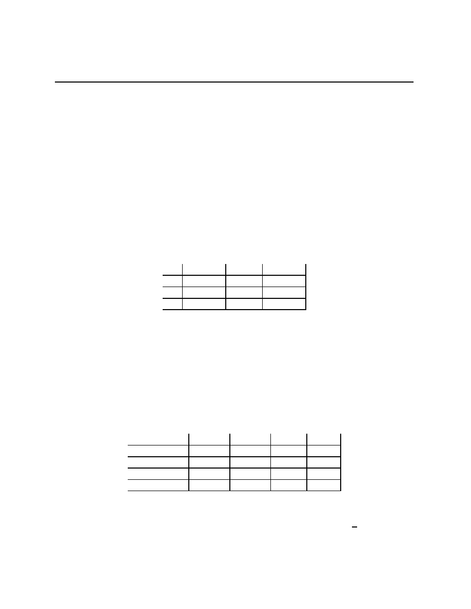
Chapter 5.9

Fix a vector of perturbations (

). If 1 is playing a strategy σ

with σ

(Up)

≥

(Up) >

0 and σ

(Down)

≥

(Down) > 0, then 2 payoffs satisfy

(σ

, Left)

≥

(Up) > 0, and u

(σ

, Right) = 0.

This means that in any perturbed game, Left strictly dominates Right for 2. Therefore, in
any equilibrium of the perturbed game, 2 puts as much mass as possible on Left, that is, 2
plays the strategy σ

(Left) = 1

−

(Right), σ

(Right) =

(Right). By symmetry, 1 puts as

much mass as possible on Up. Taking limits as (

)

→ 0, the unique perfect equilibrium

is (Up,Left).

A note here, since the

0, weak dominance turns into strict dominance in the

perturbed games. Therefore, in perfect equilibria, weakly dominated strategies are not
played.

Perfect equilibria do not survive deletion of strictly dominated strategies, an observation

due to Roger Myerson.

(1, 1)

(0, 0)

(

−1, −2)

(0, 0)

(0,

−2)

(

−2, −1) (−2, 0) (−2, −2)

Delete the two strictly dominated strategies, A

and A

and you are back at the previous

× 2 game. In the present game, (B, R) is a perfect equilibrium. To see why, suppose

that 2’s perturbations satisfy

) >

(L) and that 2 is playing the perturbed strategy

= (

(L), 1

− (

(L) +

)),

)). In this case, the payoff to T is strictly less than 0

while the payoff to B is 0. Therefore, if 1’s perturbations satisfy the parallel pattern, there
is only one equilibrium, (B, R) played with as much probability as possible. Taking limits
as the perturbations go to 0, (B, R) is perfect. After deletion of the strongly dominated
strategies, (B, R) is not perfect. Oooops.

Another example: taking expectations over Nature’s move, the 4

× 4 normal form for

the Beer-Quiche game is

(st,wk)

\(b,q)

(p, p)

(p, n)

(n, p)

(n, n)

(b, b)

(9,

−8)

(9,

−8)

(29, 0)

(b, q)

(10,

−8) (12, −9) (28, 1) (30, 0)

(q, b)

(0,

−8)

(18, 1)

(2,

−8) (20, 0)

(q, q)

(1,

−8)

(21, 0)

(1,

−8) (21, 0)

The equilibrium set for this game can be partitioned into E

and E

where

{((q, q), (0, β, 0, 1 − β)) : 21 ≥ 12β + 30(1 − β), i.e. β ≥

131

Chapter 5.9

and

{((b, b), (0, 0, β, 1 − β)) : 29 ≥ 28β + 30(1 − β) i.e. β ≥

Problem 5.24 Show that all of the equilibria in the normal form of the Beer-Quiche game
are perfect. Show the same in the agent normal form of the game.

There is a bit more theory to be had.

Theorem 5.21 (Selten) P er(Γ) is a non-empty, closed subset of Eq(Γ), and σ

∗

∈ P er(Γ)

implies that for all i

∈ I, σ

∗

) = 0.

Proof: (Non-emptiness) We have seen that P er(Γ)

6= ∅.

(Every perfect equilibrium is a Nash equilibrium) Suppose σ

∈ P er(Γ), but assume, for

the purposes of contradiction, that σ

6∈ Eq(Γ). Since σ is perfect, there exists σ

∈ Eq(Γ

→ σ as

→ 0. Since σ is not an equilibrium, there (∃i ∈ I)(∃a

∈ A

)[u

(σbackslashs

) >

(σ)]. This implies that Br

(σ) contains points strictly better than σ for i. We will show

that

(

‡) (∃N)(∀n ≥ N)[σ

(Br

(σ)) = 1

−

6∈Br

(σ)

)].

This implies that σ

(Br

(σ))

→ 1, which implies that σ

(Br

(σ)) = 1 which implies that

σ is an equilibrium, a contradiction that completes the proof.

For any s

∈ Br

(σ), continuity of the u

implies that there exists an N such that for all

≥ N, u

(σ

) > u

(σ

) for any t

6∈ Br

(σ). Since σ

∈ Eq(Γ

), this delivers (

‡).

(Perfect equilibria put no mass on weakly dominated strategies) Suppose t

∈ A

weakly dominated. Then for all

0 and all σ ∈ ×

i∈I

∆

, u

(σ

) < u

(Br

(σ)). Since

∈ Eq(Γ

), this means that σ

) =

)

→ 0. Therefore σ

) = 0.

(Closedness) For δ

∈ R

, let E

denote the closure of the set of all Eq(Γ

) where

δ · ˜1. (Note that δ < δ

implies that E

⊂ E

It is easy to check that

P er(Γ) =

∩

, that is, P er(Γ) is the the intersection of closed sets, hence closed.

The extensive form version of perfect is called “trembling hand perfection.” To get

it, just rephrase perfection using behavioral strategies. Let B

denote i’s set of behavioral

strategies, that is, B

H∈U

∆(A(H)). For each i

∈ I, let

= (

)

H∈U

where

∈ R

A(H)

Define

∈ B

: (f orallH

∈ U

)(

∀a

∈ A(H))[b

)

≥

)]

Note that if Γ is a normal form game, then B

is just ∆

For an extensive form game Γ, define Γ

to be the game (B

, u

)

i∈I

where u

is composed

with the outcome function

O(·).

Definition 5.22 b is trembling hand perfect if there exists

→ 0, b

∈ Eq(Γ

) such

that b

→ b.

132

Chapter 5.9

Often times, trembling hand perfect equilibria are simply called perfect equilibria. The-

orem 5.21 applies, except, and this is an important exception, no trembling hand perfect
equilibrium puts positive mass on any strategy that is weakly dominated in the agent normal
form of the game.

5.9.3

Properness by Myerson

A strategy σ

0 is -perfect, ∈ R

, if for all i

∈ I, σ

(Br

(σ))

≥ 1 − . It is easy to

show that σ is perfect if and only if it is the limit of

-perfect equilibria,

→ 0. An

perfect equilibrium σ is -proper if

(

∀i ∈ I)(∀a

, t

∈ A

) [[u

(σ

) < u

(σ

)]

⇒ [σ

)

≤ σ

)]] .

σ is proper if it is the limit of

-proper equilibria as

→ 0.

Properness limits the set of perturbations that are allowed and then takes the set of

limits. It has not limited the set of perturbations too far to preclude existence. Let P ro(Γ)
denote the set of proper equilibria.

Theorem 5.23 (Myerson) P ro(Γ) is a non-empty, closed subset of P er(Γ).

The proof is, to a first order of approximation, infinitely clever.

Proof: Pick

∈ (0, 1). Set

) =

/#A

for each s

∈ A

. The perturbed strategy set

∆

(

) is compact, convex and non-empty, as is the set

i∈I

∆

(

). Define the correspondence

(

·) from ×

i∈I

∆

(

) to

i∈I

∆

(

) by

(σ) =

{σ

∈ ∆

(

) : [u

(σ

) < u

(σ

)]

⇒ [σ

)

≤ σ

)]

To see that Ψ

(σ)

6= ∅, we introduce the ranking of a pure strategy a

∈ A

against σ,

defining it by

(σ, a

) = #

∈ A

: u

(σ

) > u

(σ

)

Thus, is a

∈ Br

(σ), then r

(σ, a

) = 0. Consider the mixed strategy

) =

(σ,a

)

∈A

(σ,t

)

This is clearly a mixed strategy, and it belongs to ∆

(

), so Ψ

(σ)

6= ∅. It is also fairly

easy to show that Ψ is a g.t.c., therefore it has a fixed point. The fixed point is an -proper
equilibrium.

Take a sequence

↓ 0 and a corresponding sequence σ

-proper equilibria. Taking

a subsequence if necessary, we can find a σ such that σ

→ σ because ∆ is compact.

133

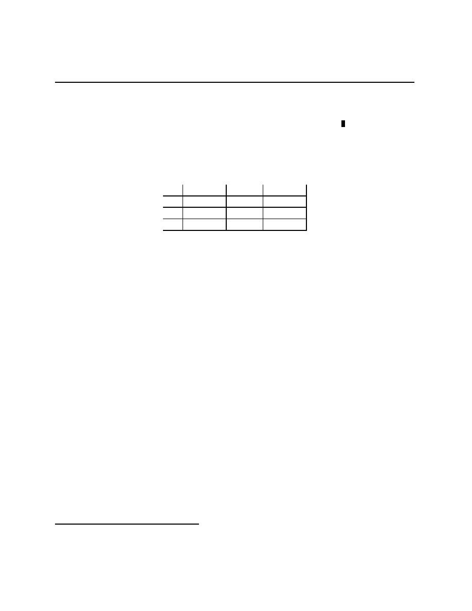
Chapter 5.9

To show that P ro(Γ) is closed, let T

be the closure of the set of δ-proper equilibria,

∈ (0, ). It is nearly immediate that P ro(Γ) = ∩

, i.e. that the set of proper equilibria

is the intersection of a collection of closed sets, hence it is itself closed.

Problem 5.25 (Optional) Show that the Ψ used in the previous proof is a gtc.

Let us reconsider the previous 3

× 3 example,

(1, 1)

(0, 0)

(

−1, −2)

(0, 0)

(0,

−2)

(

−2, −1) (−2, 0) (−2, −2)

Note that if σ

0, then for both i ∈ I for this game, and all t

6= A

, u

(σ

) < u

(σ

For an -proper equilibrium, we need to have σ

)

≤ · σ

) for both t

6= A

. The only

way to make B better than T in our calculations for (B, R) being perfect was to have

(L) >

). This cannot happen in an -proper equilibrium. Therefore, there is only

one proper equilibrium, (T, L). This survives deletion of strictly dominated strategies. There
are 3 person games for which the set of proper equilibria changes after deletion of a strictly
dominated strategy.

5.9.4

Sequential equilibria

These are a subset of the trembling hand perfect equilibria. From that point of view, they
are not exciting. What is really useful is that sequential equilibria are defined in terms of
beliefs. This change unleashed a huge torrent of creative energy in the quest for a good
refinement of Eq(Γ). Let b

0 be a strictly positive behavioral strategy. Bayes’ Law gives

beliefs, β(

·|b) at each information set H.

Definition: A strategy-belief pair, (b, β) is a sequential equilibrium if there exists

0, b

→ b such that β(·|b

)

→ β, and b is a best response to β at each H.

Seq(Γ) denotes the set of sequential equilibria.
Definition: A strategy-belief pair, (b, β) is a Bayesian Nash equilibrium if β(

·|b) is

defined by Bayes Law at all H reached with positive probability when b is played, and b is
a best response to β at each H.

Give some examples, emphasizing the beliefs at H that arise from Bayes Law and b

Every trembling hand perfect equilibrium is sequential, but not the reverse. Consider

the following game

Oh well, we need more work if we are to get

S’s that satisfy the self-referential tests above.

134

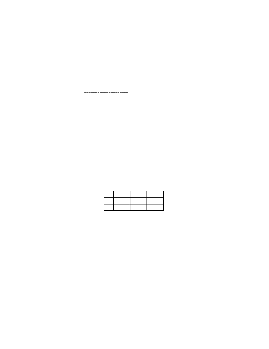
Chapter 5.9

•

Problem 5.26 Show that P er(Γ)

( Seq(Γ) = Eq(Γ) in the above game.

5.9.5

Strict perfection and stability by Kohlberg and Mertens

A strategy σ is strictly perfect if for all sequences Γ

→ 0, there exists a sequence

∈ Eq(Γ

) such that σ

→ σ.

Strictly perfect equilibria do not always exist, e.g.

(1, 1)

(1, 0)

(0, 0)

(1, 1)

(0, 0)

(1, 0)

In this game, P ro(Γ) = P er(Γ) = Eq(Γ), so none of the refinements work here. Perhaps

they shouldn’t, but in any case, it is easy to show that there is no strictly perfect equilibria,
just take

(M ) >

(R) > 0,

(M )

→ 0. The only limit of equilibria of these perturbed

games is (T, L). Now take

(R) >

(M ) > 0,

(R)

→ 0. The only limit of equilibria of

these perturbed games is (B, L). Oooops, no strictly perfect equilibrium.

If x is a point and F is a set, define d(x, F ) = inf

{d(x, f) : f ∈ F }.

Definition: A closed set E

⊂ Eq(Γ) has property (SP) if it satisfies

(SP) for all sequences Γ

→ 0, there exists a sequence σ

∈ Eq(Γ

) such

that d(σ

, E)

→ 0.

Problem 5.27 Show that if E =

{σ} and E satisfies (SP), then σ is strictly perfect.

Problem 5.28 Show that for all Γ, Eq(Γ) satisfies (SP). (If this is too daunting, just show
it for two non-trivial games.)

135

Chapter 5.9

In light of the last problem, what is needed is a smallest closed set E with property (SP).
Definition: A closed E

⊂ Eq(Γ) is K-M stable if it satisfies Condition SP and no closed,

non-empty, proper subset of E satisfies Condition SP.

In the 2

× 3 game above, we see that the unique K-M stable set is {(U, L), (R, L)}, i.e.

it is not connected.

Time for the quick detour about connectedness. A set E

⊂ R

is path-connected

if for all x, y

∈ E, there is a continuous function f : [0, 1] → E such that f(0) = x and

f (1) = y. Intuitively, this means that you can draw a continuous path from x to y that
stays inside of E. It is clear that all convex sets are path-connected. It is also clear that
if E and E

are path-connected and E

∩ E

6= ∅, then E ∪ E

is path-connected, though

∩ E

may not be. There is a difference between connected and path-connected, and every

path-connected set is connected. I am not going to tell you about the distinction because
for our purposes path-connected is enough. However, this is a warning that when you see
proofs of connectedness in the literature, you may not recognize the concept.

Look at Faruk Gul’s example.

5.9.6

Stability by Hillas

Define the Hausdorff distance between two compact sets K

and K

, K

) = inf

{ > 0 : K

⊂ K

, and K

⊂ K

where K

∪

x∈K

B(x, ) is the open -ball around K.

Define the Hillas distance between two gtc’s mapping K to K by

d(Ψ, Ψ

) = max

x∈X

(Ψ(x), Ψ

(x)).

Definition: A closed set E

⊂ Eq(Γ) has property (S) if it satisfies

(S) for all sequences of gtc’s Ψ

, d(Ψ

, Br)

→ 0, there exists a sequence σ

fixed points of Ψ

such that d(σ

, E)

→ 0.

Definition: A closed set E

⊂ Eq(Γ) is (Hillas) stable if it satisfies (S) and no closed,

non-empty, proper subset of E satisfies (S).

This is often said as “E is (Hillas) stable if it is minimal with respect to property (S).”
In the 2

× 3 game that we used to demonstrate that strictly perfect equilibria do not

exist, it is (perhaps) possible to visualize the perturbations that Hillas uses. It is a good
exercise to show that ((1/3, 2/3), (1, 0, 0)) is the limit of fixed points of Ψ’s close to Br.

136

Chapter 5.10

Theorem 5.24 (Hillas) There exist a non-empty stable set E of equilibria. Further, E is
connected, satisfies the self-referential tests given above, is a subset of P er(Γ), and P ro(Γ)

∩

6= ∅.

In practice, the way that this is used is to (1) find the connected sets of equilibria and (2)

test whether or not they fail the various criteria. For example, if a connected set E contains
strategies that put positive mass on weakly dominated strategies, then E

6⊂ P er(Γ), and so

E is not (Hillas) stable. If none of the proper equilibria belong to E, then E is not (Hillas)
stable. If those tests don’t work, and they often don’t in signaling games, then you can turn
to the self-referential tests. If you know that all but one of the connected sets of equilibria
fails the criteria, then the existence part of the above theorem tells you that the remaining
one must be (Hillas) stable. Directly checking stability can be difficult.

5.10

Signaling game exercises in refinement

Here are a variety of signaling games to practice with. The presentation of the games is
a bit different than the extensive form games we gave above, part of your job is to draw
extensive forms. Recall that a pooling equilibrium in a signaling game is an equilibrium
in which all the different types send the same message, a separating equilibrium is one in
which each types sends a different message (and can thereby be separated from each other),
a hybrid equilibrium has aspects of both behaviors.

The presentation method is taken directly from Banks and Sobel’s (1987) treatment of

signaling games. Signaling games have two players, a Sender S and a Receiver R. The Sender
has private information, summarized by his type, t, an element of a finite set T . There is
a strictly positive probability distribution ρ on T ; ρ(t), which is common knowledge, is the
ex ante probability that S’s type is t. After S learns his type, he sends a message, m, to R;
m is an element of a finite set M . In response to m, R selects an action, a, from a finite set
A(m); S and R have von Neumann-Morgenstern utility functions u(t, m, a) and v(t, m, a)
respectively. Behavioral strategies are q(m

|t), the probability that S sends the message m

given that his type is t, and r(a

|m), the probability that R uses the pure strategy a when

message m is received. R’s set of strategies after seeing m is the #A(m)

− 1 dimensional

simplex ∆

, and utilities are extended to r

∈ ∆

in the usual fashion. For each distribution

λ over T , the receiver’s best response to seeing m with prior λ is

Br(λ, m) = arg max

r(m)∈∆

t∈T

v(t, m, r(m))λ(t).

(5.1)

Examples are represented with a bi-matrix B(m) for each m

∈ M. There is one column

in B(m) for each strategy in A(m) and one row for each type. The (t, a)’th entry in B(m) is

137

Chapter 5.10

(u(t, m, a), v(t, m, a)). With t

being the strong type, t

the weak, m

being beer, m

being

quiche, a

being pick a fight, and a

being not, the Beer-Quiche game is

B(m

)

10,

−10

30, 0

0, 10

20, 0

B(m

)

−10

20, 0

10, 10

30, 0

You should carefully match up the parts of this game and the extensive form of B-Q

given above.

Here is a simple example to start on:

B(m

)

2, 2

B(m

)

3, 3

0, 0

3, 3

Problem 5.29 Draw the extensive form for the game just specified. Find the 3 connected
sets of equilibria. Show that all equilibria for this game are both perfect and proper. Show
that the 3 connected sets of equilibria are both Hillas and K-M stable.

The following game is Cho’s (1987, Example 2.1): the types are A, B, and C, ρ(A) =

ρ(C) = 3/8, ρ(B) = 1/4, the messages are L and R, and the actions are as given.

B(L)

2, 1

−1, 0

2, 1

0, 0

2, 0

0, 1

B(R)

0, 2

0, 0

0, 2

4, 3

−1

−3

−2

4, 0

Problem 5.30 Draw the extensive form for the game just specified and analyze the equilib-
rium set.

The following is a sequential settlement game of a type analyzed by Sobel (1989): There

are two types of defendants, S: type t

defendants are negligent, type t

defendants are not,

ρ(t

) = 1/2. S offers a low settlement, m

, or a high settlement, m

. R, the plaintiff, either

accepts, a

, or rejects a

. If R accepts, S pays R an amount that depends on the offer but

not S’s type. If R rejects the offer, S must pay court costs and a transfer depending only
on whether or not S is negligent. With payoffs, the game is

B(m

)

−3, 3

−6, 0

−3, 3

−11, 5

B(m

)

−5, 5

−6, 0

−5, 5

−11, 5

138

Chapter 5.10

Problem 5.31 Draw the extensive form for the game just specified. Analyze the equilibria
of the above game, picking out the perfect, the proper, the sequential, and the Hillas stable
sets.

One more game! This one has ρ(t

) = 0.4.

B(m

)

0, 0

B(m

)

−1, 3

−1, 2

1, 0

−1, −2

1, 0

1, 2

−2, 3

Problem 5.32 Draw the extensive form for the game just specified. Find the pooling and
the separating equilibria, if any, check the perfection and properness of any equilibria you
find, and find the Hillas stable sets.

Problem 5.33 A little more practice with sequential equilibria.

This game has two kinds of Nash equilibria, one kind involves player 1 playing down,

that is, playing D

, the other involves player 1 playing across, that is, playing A

One of the equilibria in which 1 plays D

is (D

, A

, L

), i.e. the behavioral strategy

π = (π

, π

) = ((1, 0), (0, 1), (1, 0))

where the following table contains the key to reading these 1’s and 0’s

Player

Strategy

= (π

), π

))

= (π

), π

))

= (π

), π

))

139

Chapter 5.10

1. Find the set of π

and π

for which ((1, 0), π

, π

) is a Nash equilibrium.

2. Show that none of the π

you found in the previous problem is part of a sequential

equilibrium.

3. Find the set of Nash equilibria in which 1 plays π

= (0, 1), that is, in which 1 plays

4. Find the set of beliefs, that is, (µ

, µ

), µ

= 1

− µ

, for 3 for which L

is a strict best

response, for which R

is a strict best response, and for which 3 is indifferent between

and R

5. Show that all of the Nash equilibria of Exercise 3 are sequential.

Problem 5.34 Yet more practice with sequential equilibria. Consider a market with one
incumbent firm and a potential entrant. The potential entrant has low costs with probability
0.2, and has high costs with probability 0.8. The actual costs (low or high) of the entrant
are private information to the entrant, who decides whether to stay “out” or “enter.” The
outside option for the low cost entrant has an expected utility of 25, while the outside option
for the high cost entrant has an expected utility of 0. If the potential entrant stays out,
then the incumbent has an expected utility of 25. If the potential entrant enters, then the
incumbent decides whether to “fight” or “acquiesce.” If the incumbent fights, then the payoffs
for the entrant and incumbent respectively are (20,

−25) when the entrant is low cost, and

(

−10, 40) when the entrant is high cost. If the incumbent acquiesces, then the payoffs are

(40, 10) when the entrant is low cost, and (20, 36) when the entrant is high cost.

One version of the game tree for this game is

low

high

0.2

0.8

entrant

out

enter

incumbent

100

−25

−10

140

Chapter 5.10

1. A separating equilibrium is one in which all the different types of Senders take

different actions, thereby separating themselves from each other. A pooling equilib-
rium is one in which all the different types of Senders take the same action. Show
that the only Nash equilibria of this game are pooling equilibria, and that all of them
are sequential.

2. Show that one of the sequential equilibria of the previous game is still a Nash equilib-

rium, but is not sequential in the following, changed version of the above game.

low

high

0.2

0.8

entrant

out

enter

incumbent

100

−25

−10

141

Chapter 5.10

142

Chapter 6

Repeated Games

Here we take a game Γ = (A

, u

)

i∈I

and play it once at time t = 1, reveal to all players

which a

∈ A

each player chose, then play it again at time t = 2, reveal, etc. until N plays

have happened, N

≤ ∞.

The basic observation is, roughly, “repeating games can greatly expand the set of equi-

libria.” This section of the course is devoted to making this statement meaningful and
qualifying it.

There are four basic kinds of reasons to study what happens in repeated games, they

are not mutually exclusive. First, it delivers an aesthetically pleasing theory. Second, it has
the benefit of making us a bit more humble in our predictions. Third, we believe that many
of the most interesting economic interactions are repeated many many times, it is good to
study what happens in these games. Fourth, economics, and equilibrium based theories
more generally, do best when analyzing routinized interactions. In game theory models,
routinized interactions makes it easier to believe that each i has figured out not only that
they are solving the problem

max

∈∆(A

)

(σ

∗

\σ

but that the solution is σ

∗

. Don’t take the last reason too seriously, the theory of repeated

games we will look at first is not particularly good for analyzing how people might arrive
at solving the equilibrium maximization problem.

6.1

The Basic Set-Up and a Preliminary Result

When playing the game N <

∞ times, the possible history space for the game is H

, the

product space

= S

× . . . × S

}

N times

143

Chapter 6.1

For any h

= (s

, . . . , s

, s

t+1

, . . . , s

)

∈ H

, i’s payoffs are

) =

N
t=1

When playing the game “infinitely often”, the possible history space is

∞

= (s

, s

, . . .)

∈ S × S × · · · ,

and the payoffs are discounted with discount factor δ,

∞

) =

1−δ

∞
t=1

The important point about these payoffs is that they are on the same scale as u, specifically,
for all N and all δ,

u(S)

⊂ U

), u(S)

⊂ U

∞

), and

)

⊂ co (u(S)), U

∞

)

⊂ co (u(S)).

These are true because in all cases, the weights on the u

) add up to 1, 1 = 1,

1−δ

∞
t=1

1, and 1/N +

· · · + 1/N

}

times

= 1. The following will be important several times below.

Problem 6.1 For all v

∈ co (u(S)) and for all > 0,

(

∃N

)(

∀N ≥ N

)(

∃h

∈ H

)

− vk < , and

(

∃δ < 1)(∃h

∞

∈ H

∞

)(

∀δ ∈ (δ, 1)kU

∞

)

− vk < .

As always, strategies are complete contingent plans. For completeness, we define H

as a one-point set, H

}. A behavioral strategy for i is, for every t ∈ {1, . . . , N}, a

mapping

: H

t−1

→ ∆

so that a strategy for i is a sequence σ

= (σ

)

t=1

, and Σ

is the set of all behavioral

strategies. Each vector behavioral strategy σ = (σ

)

i∈I

, specifies an outcome distribution

over H

, denoted by

O(σ). Playing the strategy σ starting from a history h

t−1

∈ H

t−1

gives

the outcome

O(σ|h

t−1

Summarizing, for N <

∞,

= (Σ

, U

)

i∈I

for N =

∞,

∞

= (Σ

∞

, U

)

i∈I

144

Chapter 6.2

A vector σ

∗

is an equilibrium if the usual conditions hold, and the set of equilibria is

Eq(Γ

) or Eq(Γ

∞

) as N <

∞ or N = ∞. A vector σ

∗

is a sub-game perfect equilibrium if

it is a Nash equilibrium given any starting history h

t−1

, t

∈ {1, . . . , N}. The set of sub-game

perfect equilibria is SGP (Γ

) or SGP (Γ

∞

) as N <

∞ or N = ∞.

Since the strategy sets are very different in Γ, Γ

, and Γ

∞

, the way that we will

be comparing the equilibrium sets is to compare u(Eq(Γ)), U

(Eq(Γ

)), U

(SGP (Γ

)),

∞

(Eq(Γ

∞

)) and U

∞

(SGP (Γ

∞

)). The starting point is

Lemma 6.1 If σ

∗

∈ Eq(Γ), then σ

≡ σ

∗

∈ SGP (Γ

), i

∈ I, t = 1, . . . , N, and σ

≡ σ

∗

∈

SGP (Γ

∞

), i

∈ I, t = 1, 2, . . ..

Since every SGP is an equilibrium and Eq(Γ)

6= ∅, immediate corollaries are

∅ 6= u(Eq(Γ)) ⊂ U

(SGP (Γ

))

⊂ U

(Eq(Γ

)), and

∅ 6= u(Eq(Γ)) ⊂ U

∞

(SGP (Γ

∞

))

⊂ U

∞

(Eq(Γ

∞

)).

In this sense, we’ve “rigged the game,” all that can happen is increase in the set of

equilibria when the game is repeated.

6.2

Prisoners’ Dilemma finitely and infinitely

To get a flavor of what will happen in this section, we will look at repeating the Prisoners’
Dilemma game Γ from above.

Squeal

Silent

Squeal

(

−B + r, −B + r) (−b + r, −B)

Silent

(

−B, −b + r)

(

−b, −b)

Problem 6.2 Show that

O(Eq(Γ

)) contains only one point when N <

∞. Show that

SGP (Γ

) contains only one point when N <

∞.

One way to work the next problem uses “Grim Trigger Strategies,” that is, σ

(Silent, Silent), and for t

≥ 2, σ

t−1

) = Silent if h

t−1

is all Silent, and is equal to Squeal

for all other h

t−1

Problem 6.3 Show that there exists a δ <

1 such that for all δ

∈ (δ, 1), O(SGP (Γ

∞

))

contains the history in which each player plays Silent in each period.

145

Chapter 6.2

The grim trigger strategies are a special case of what are called “Nash reversion” strate-

gies — pick a Nash equilibrium τ for Γ and a vector s

∈ S. Nash reversion strategies are

= s, and for t

≥ 2,

t−1

) =

if h

t−1

= (s, s, . . . , s)

otherwise

In this game, the only τ

∈ Eq(Γ) is (Squeal, Squeal).

Summarizing what we have seen in the repeated prisoners’ dilemma so far, for all N <

∞

and for all δ sufficiently close to 1,

u(Eq(Γ)) = U

(Eq(Γ

)) = U

(SGP (Γ

))

( U

∞

(SGP (Γ

∞

)).

What is a bit puzzling is the question, “Why is there so large a distinction between Γ

for large N and Γ

∞

for δ close to 1?” This is puzzling because both types of games are

supposed to be capturing interactions that are repeated many many times.

Roy Radner had a solution for the puzzle in the case of the repeated Prisoners’ Dilemma.

His solution was later (considerably) generalized by Fudenberg and Levine. Both papers
worked with Herbert Simon’s satisficing. Radner worked with the definition of satisficing
having to do with solving optimization problems to within some > 0 of the optimum
achievable utility. Fudenberg and Levine replaced complicated optimization problems by
simpler ones. This is Simon’s other notion of satisficing. Fudenberg and Levine then showed
that, in games more general than the repeated games we’re looking at, this gives Radner’s
version of satisficing.

Definition (Radner): For a game γ = (T

, v

)

i∈I

and an

≥ 0, a strategy vector σ is an

-equilibrium if

(

∀i ∈ I)(∀t

∈ T

)[u

(σ)

≥ u

(σ

)

− ].

If = 0, an -equilibrium is an equilibrium. One can (and you should) write down the
definition of an -SGP.

Radner showed that for every > 0, there exists an N

such that for all N

≥ N

, there

exists strategies σ

∈ SGP (Γ

) with the property that

O(σ) involves (Silent, Silent) at all

time periods. One part of Fudenberg and Levine’s work considered a subclass of strategies
for a repeated game Γ

∞

. The subclass consisted of strategies of the form “stop thinking

about what to do after N periods.” They showed that the set of limits of -SGP in these
strategies, limits being taken as

→ 0 and N → ∞, give exactly the SGP of Γ

∞

. Further,

equilibria within these subclasses are -SGP’s.

In any case, using either logic, and variants the trigger strategies discussed above it is

possible to show that, for Γ being the Prisoners’ Dilemma,

Theorem 6.2 If v > u(Squeal, Squeal) and v

∈ co (u(S)), then for all > 0,

146

Chapter 6.3

1. exists N

such that for all N

≥ N

, B(v, )

∩ U

(SGP

(Γ

))

6= ∅, and

2. there exists a δ < 1 such that for all δ

∈ (δ, 1), B(v, ) ∩ U

∞

(SGP (Γ

))

6= ∅.

So, those are the major patterns for the results, the equilibrium sets expand as N grows

large or as δ

↑ 1, and the utilities of the approximate equilibrium set for Γ

, N large, look

like the utilities for Γ

∞

, δ

' 1.

Radner offered a couple of rationales for -equilibria with > 0, and it worth the time

to reiterate his points.

1. First, actually optimizing is quite hard and we might reasonably suppose that people

only optimize their payoffs to within some small .

Herbert Simon distinguished

between approximately optimizing in this sense, and in exactly optimizing a simplified
version of the problem. In this game, we might consider looking for equilibria in
some more limited class of strategies, e.g. in a class that contains the one called “tit-
for-tat” — start by playing cooperatively and otherwise match your opponent’s last
play, and other simpleminded strategies. (I told you game theory often captured
the subtle dynamics of a kindergarden classroom.) This second approach has been
modeled extensively by assuming that players are limited in a number of aspects, most
prominently by Abreu and Rubinstein who assumed that they are “finite automata”.

2. Second, and more intriguingly, Radner argued that we might believe that the players

in this game understand that if both optimize all the way, if both squeeze out the last
little bit of surplus, then a disaster will befall them both. It seems to me that this is an
argument about socialization towards Pareto dominant outcomes — for the common
good I am willing to sacrifice a little bit. This seems reasonable, but one might argue
that if this is true, then it ought to show up in the payoffs. A really rigid version of
this argument would say that if it is hard to put this into the payoffs convincingly (it
is) then this indicates that we don’t really understand what’s behind this argument.
One way to understand what is going on is to think about the advantages of having
a reputation for being a good citizen. In other words, any game should be thought of
as being imbedded in a larger social context.

6.3

Some results on finite repetition

Now let Γ be the tragedy of the Commons game as given (a long ways) above. The two
claims we will look at are
Claim: If h

∈ O(Eq(Γ

)), then at the N ’th time period, h specifies the static Nash

equilibrium.

This is a special case of

147

Chapter 6.4

Lemma 6.3 In the last period of equilibrium play of Γ

, a static Nash equilibrium is played.

This implies that complete efficiency cannot be achieved as part of a Nash equilibrium

of Γ

, though one could get the efficient outcome in periods t = 1, 2, . . . , N

− 1, which is

pretty close. One could have all countries (players) playing the strategy

start by playing 1/I times the efficient fleet size, continue playing this so long as
everyone else does and t

≤ N − 1, if at t ≤ N − 1, some country i has deviated

from 1/I-times the efficient fleet size at any point in the past, then identify the
first deviator breaking ties by alphabetizing (in Swahili), have everyone who is
not the first deviator play 1/(I

− 1) times the total fleet size that yields 0 profits

at t + 1, have the deviator play fleet size of 0, and at t = N , if there has been
no deviation from 1/I times the efficient fleet size, play the static game Nash
equilibrium fleet size.

Problem 6.4 Give conditions on the payoffs U

for which the strategies just described

belong to Eq(Γ

Something peculiar is happening, the Tragedy of the Commons and the Prisoners’

Dilemma, played once, have just one equilibrium, however, when played N <

∞ times,

the Tragedy has many equilibria, the Dilemma just one. It is possible to explain this using
the language of “threats.”

6.4

Threats in finitely repeated games

Put equilibrium considerations in the back of your mind for just a little bit, and cast your
memory back (fondly?) to those school year days spent in terror of threats by older, larger
kids. Consider the question, “What is the worst that players j

6= i can do to player i?”

Well, they can call him/her a booby or a nincompoop, but these are not sticks nor stones,
and given that we are now adults, we are not supposed to believe that this hurts too much.
However, stealing your lunch money and stuffing you into a garbage can, now that hurts.
What j

6= i can do is get together and agree to take those actions that make i so miserable

as possible. This is a threat with some teeth to it. Now, i has some protection against this
behavior — knowing that the others are ganging up, i can plan accordingly to maximize i’s
utility against the gang-up behavior. There are three “safe” utility levels that one might
imagine i being able to guarantee iself,

pure
i

= min

−i

∈×

j6=i

max

∈A

, s

−i

mixed

= min

−i

∈×

j6=i

∆(A

)

max

∈A

, σ

−i

), and

148

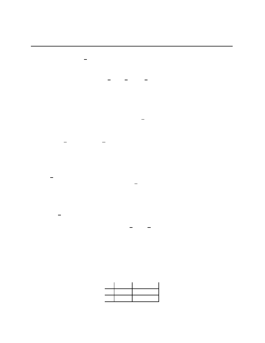
Chapter 6.4

corr

= min

−i

∈∆(×

j6=i

)

max

∈A

, µ

−i

Since

j6=i

⊂ ×

j6=i

∆(A

)

⊂ ∆(×

j6=i

pure
i

≥ v

mixed

≥ v

corr

Problem 6.5 Give games where the two inequalities are strict.

The first corresponds of the worst that dolts who do not understand randomization can

do to i, the second corresponds of the worst that enemies who do understand independent
randomization can do to i, the third corresponds of the worst that fiends who completely
understand randomization can do to i. The three v

’s are called “safety levels.” Here is one

of the reasons.

Lemma 6.4 For all i

∈ I and for all N (for all δ), if σ is an equilibrium for Γ

(for Γ

∞

then U

(σ)

≥ v

mixed

∞

δ,i

(σ)

≥ v

mixed

This lemma is ridiculously easy to prove once you see how. Suppose that other players

are playing some strategy σ

−i

. In period 1, have i play a myopic, that is, one period best

response to the distribution over A

−i

induced by σ

−i

, σ

∈ Br

(σ

)). More generally,

after any h

t−1

, have i play σ

∈ Br

(σ(h

t−1

). In each period, it must be the case that

)

≥ v

mixed

The following is a pair of reasons to call the v

’s safety levels, neither proof is particularly

easy.

Theorem (Benoit & Krishna): Suppose that for each i

∈ I there is a pair of equilibria

∗

(i) and σ

(i) for Γ such that u

(σ

∗

(i)) > u

(σ

(i)). Suppose also that the convex hull of

u(S) has non-empty interior. Let v be a vector in the convex hull of u(S) such that for all
i

∈ I, v

> v

pure
i

. Then for all > 0, there exists an N

such that for all N

≥ N

, there

is a subgame perfect Nash equilibrium σ

∗

of Γ

such that

ku(σ

∗

)

− vk < . If the words

“subgame perfect” are deleted, then change v

pure
i

to v

mixed

It is intuitive for two reasons, one obvious and one a bit more subtle, that more things

are possible when we look at equilibria rather than subgame perfect equilibria. First, there
are more equilibria than there are subgame perfect equilibria, this is obvious. Second, some
of the strategies that go into the proof require players to min-max someone else, and this
can be rather costly. In an equilibrium, one can threaten to min-max someone and never
have to seriously consider carrying through on it. But for an equilibrium to be subgame
perfect, it must only consider min-max threats that are seriously considered as possibilities.
Let us look at both these points in the following 2

× 2 game,

(2,9)

(-20,-80)

(10,0)

(-30,-100)

149

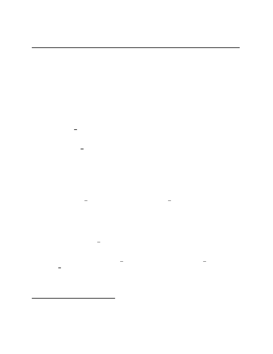
Chapter 6.5

For this game, Eq(Γ) = (B, L) and u(Eq(Γ)) = (10, 0).

Claim:

O(Eq(Γ

)) contains the history h = ((T, L), (B, L)).

It is important to note that (T, L) is nothing like the unique equilibrium of Γ. The claim

can be seen to be true by considering the strategies σ

) = (T, L), σ

)

≡ B, and

) =

if h

= (T, L)

otherwise

These are in fact Nash equilibria, just check the mutual best response property. They are
not subgame perfect equilibria, just check that they call for play of a dominated strategy in
the case of “otherwise.” That is the obvious reasoning.

Show that the v

pure
i

are (

−20, 0) for this game. The more subtle observation is that for

2 to min-max 1, 2 must suffer a great deal. To have a subgame perfect equilibrium in which
1’s utility is held down, we must have strategies in which it regularly happens that some
s

giving 2 u

) < v

pure

happens. Therefore, the strategies for the Benoit and Krishna

result must also threaten the threateners. In subgame perfect equilibrium strategies, 2 must
be threatened with dire consequences, and it must be an equilibrium threat, after s/he has
avoided receiving a period’s worth of

−80 or −100. In particular, s/he must be threatened

by something even worse that what s/he was getting by going along with the strategies. In
equilibrium strategies, 2 must be threatened with dire consequences, but it needn’t be an
equilibrium threat.
Claim: Let v be a vector in the convex hull of u(S), co (u(S)). If v

(−20, 0), then for

any > 0, there exists δ < 1 such that if for all i

∈ I, δ

∈ (δ, 1), then

(

∃v

∈ u(O(Eq(Γ

∞

(δ))))[

− vk < ].

6.5

Threats in infinitely repeated games

The third reason to call the v

’s safety levels appears in the following result, which we will

not prove, though we will talk about it.

Folk Theorem: Suppose that co (u(S)) has non-empty interior. Let v be a vector in
co (u(S)) such that for all i

∈ I, v

> v

mixed

. For all > 0, there exists a δ < 1 such that

for all δ

∈ (δ, 1),

B(v, )

∩ U

(SGP (Γ

∞

))

6= ∅.

Before discussing how the proof works, let look at an example violating the condition

that co (u(S)) have non-empty interior, in particular, let us look at the Matching Pennies

We will not even state the most general version of this result, for that see Lones Smith (19??,

Econometrica).

150

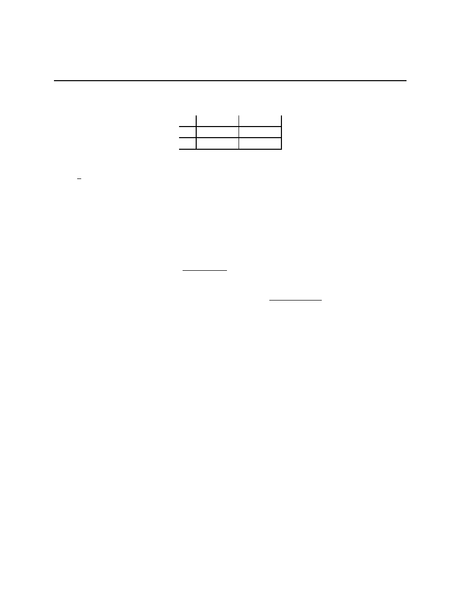
Chapter 6.6

game,

(+1,

−1) (−1, +1)

(

−1, +1) (+1, −1)

Claim: For all δ

∈ (0, 1)

, if σ

∞

∈ Eq(Γ

∞

(δ)), then

O(σ

∞

) is the i.i.d. distribution putting

mass

on each point in S in each period. In this game, there is no v

∈ co (u(S)) that is

greater than the threat point vector (0, 0).

Three person example violating the interiority condition goes here.

Problem 6.6 This question concerns infinitely repeated Cournot competition between two
firms with identical, constant marginal costs, c > 0, identical discount factors, 0 < δ < 1,
and a linear demand curve with intercept greater than c.

1. For what range of δ’s can monopoly output be a subgame perfect equilibrium with

Nash reversion strategies?

2. Show that as δ

↑ 1, prices arbitrarily close to the competitive price c also arises as

part of the equilibrium price path.

6.6

Rubinstein-St˚

ahl bargaining

Two people, 1 and 2, are bargaining about the division of a cake of size 1. They bargain
by taking turns, one turn per period. If it is i’s turn to make an offer, she does so at the
beginning of the period. The offer is α where α is the share of the cake to 1 and (1

− α)

is the share to 2. After an offer α is made, it may be accepted or rejected in that period.
If accepted, the cake is divided forthwith. If it rejected, the cake shrinks to δ times its size
at the beginning of the period, and it becomes the next period. In the next period it is j’s
turn to make an offer. Things continue in this vein either until some final period T , or else
indefinitely.

Suppose that person 1 gets to make the final offer. Find the unique subgame perfect

equilibrium. Suppose that 2 is going to make the next to last offer, find the unique subgame
perfect equilibrium. Suppose that 1 is going to make the next to next last offer, find the
subgame perfect equilibrium. Note the contraction mapping aspect and find the unique
solution for the infinite length game in which 1 makes the first offer.

Problem 6.7 The Joker and the Penguin have stolen 3 diamond eggs from the Gotham
museum. If an egg is divided, it loses all value. The Joker and the Penguin split the eggs

151

Chapter 6.9

by making alternating offers, if an offer is refused, the refuser gets to make the next offer.
Each offer and refusal or acceptance uses up 2 minutes. During each such 2 minute period,
there is an independent, probability r, r

∈ (0, 1), event. The event is Batman swooping in

to rescue the eggs, leaving the two arch-villains with no eggs (eggsept the egg on their faces,
what a yolk). However, if the villains agree on a division before Batman finds them, they
escape and enjoy their ill-gotten gains.

Question: What does the set of subgame perfect equilibria look like? [Hint: it is not in

your interest to simply give the Rubinstein bargaining model answer. That model assumed
that what was being divided was continuously divisible.]

6.7

Optimal simple penal codes

Here we are going to examine the structure of the subgame perfect equilibria of infinitely
repeated games.

6.8

Abreu’s example

We will take this directly from his paper.

6.9

Harris’ formulation of optimal simple penal codes

Time starts at t = 1, at each stage the simultaneous game Γ = (A

, u

)

i∈I

is played, A

is sequentially compact with metric ρ

, and u

is jointly continuous with respect to any of

metrics ρ inducing the product topology. For a history (read vector) h

∈ H = ×

∞

t=1

S, h

denotes the t’th component of h, payoffs are given by

(h) =

∞

t=1

where 0 < δ

< 1. The product topology of H can be metrized by

d(h, h

) =

∞

t=1

min

−n

, ρ(h

, h

)

} .

Problem 6.8 The set H is sequentially compact in the metric d, and each U

is continuous.

Player i’s strategy for period t is a function σ

: H

t−1

→ A

where H

t−1

k=1

S, and

is, by convention, some one point set. An initial history is a vector h

∈ H

. Player

152

Chapter 6.9

i’s strategy is the vector σ

= (σ

, σ

, . . .). A profile of strategies for the players is then

σ = (σ

)

i∈I

, and a profile of strategies at time t is σ

= (σ

)

i∈I

Let

O(σ, h, t) denote the outcome h for the first t time periods followed by the outcome

determined by play of σ. Thus, (

O(σ, h, t))

= h

for 1

≤ k ≤ t, and

(

O(σ, h, t))

= σ

((

O(σ, h, t))

, (

O(σ, h, t))

, . . . , (

O(σ, h, t))

k−1

)

for k > t.
Definition: A strategy combination σ is a subgame perfect equilibrium of the re-
peated game if (

∀i, t, h) and for all strategies γ

for i,

((

O(σ, h, t))) ≥ U

((

O(σ\γ

, h, t))).

The assumption is that the repeated game has a subgame perfect equilibrium in pure

strategies.
Definition: For a strategy vector σ, the history q

∈ H comes into force in period t + 1

after a given initial history h

= (h

, . . . , h

) of

O(σ, h, t) = (h

, . . . , h

, q

, . . .).

Given histories in H, q

and (q

)

i∈I

, the following recursive construction of a strategy

vector F (q

, q

, . . . , q

) will be used many times below:

1. q

comes into force in period 1.

2. If q

, 0

≤ j ≤ I came into force in period k, if q

isfollowed in all periods up to but

not including period t

≥ k, and if player i deviates againts q

t−k+1

in period t, then q

comes into force in period t + 1.

3. If q

came into force in period k, and more than 1 player deviated against q

t−k+1

period t

≥ k, then q

comes into force in period t + 1 where i is the lowest numbered

amongst the deviating players.

Definition: A simple penal code is a vector of histories (q

)

i∈I

. A simple penal code is

perfect if there exists q

∈ H such that F (q

, q

, . . . , q

) is a subgame perfect equilibrium.

Problem 6.9 If (q

)

i∈I

is perfect, then (

∀i ∈ I)[F (q

, q

, . . . , q

)] is a subgame perfect equi-

librium.

Let P

⊂ H denote the set of outcomes associated with subgame perfect equilibria. Let

denote inf

(q) : q

∈ P }.

Definition: A simple penal code (q

)

i∈I

is optimal if it is perfect and if

(

∀i ∈ I)[U

) = U

153

Chapter 6.10

Lemma: Let f = F (q

, q

, . . . , q

). If no single period deviation against f is profitable for

any player in any subgame, then f is a subgame perfect equilibrium.

Problem 6.10 Show that (q

)

i∈I

is a perfect simple penal code if and only if for all i, j, t,

and all a

∈ A

∞

k=t

)

≥ δ

) + δ

Proposition: There exists an optimal simple penal code.
Proposition: If (q

)

i∈I

is an optimal simple penal code, then

(

∀q

∈ P )[F (q

, q

, . . . , q

) is a subgame perfect equilibrium].

6.10

“Shunning,” market-place racism, and other ex-
amples

Again, we will work through a problem.

Problem 6.11 There are N identical, incumbent firms Bertrand (price) competing in an
industry. The industry (inverse) demand curve is p = 1

− q. Each incumbent firm has

the constant marginal cost function C(q

) = cq

for some 0 < c

1. The consumers

react instantly to price changes, going to the lowest cost supplier, evenly dividing themselves
among firms tied at the lowest price. For the repeated versions of this game, the firms have
the same discount factor, β

∈ (0, 1).

1. Find the one-shot Bertrand-Nash equilibrium prices, quantities, and profits for this

industry.

2. (Nash reversion) As a function of β, find the highest price (i.e. most collusive) q

such

that F (q

, q

, . . . , q

) is a subgame perfect equilibrium where (q

, . . . , q

) is the Nash

equilibrium.

3. (Temporary Nash reversion) Let p

denote the price that a monopolist would charge

in this industry and let π

> 0 denote industry monopoly profits. For each i

∈ I, let

be the history

= ( ~c, . . . , ~c

| {z }

periods

, ~

, . . .)

154

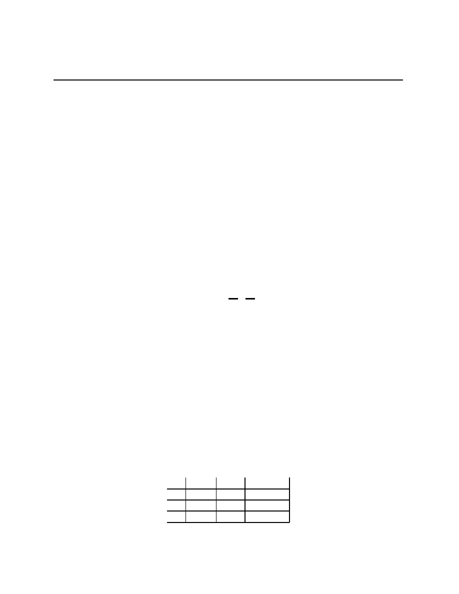
Chapter 6.10

where ~

x is an I-length vector with x in each component. Let q

be the history

= (p

, p

, . . .).

Show that for β close to 1 and T large, F (q

, q

, . . . , q

) is a subgame perfect equi-

librium. (Verbally, these strategies are “play c for T periods if there is ever a price
gouger.”)

4. (Discriminatory equilibria) Now suppose that any of the firms could lower their costs

to C(q

) = rcq

with 0 < r < 1 by hiring, at a lower wage, members of an oppressed

racial, ethnic, gender, or religious group. Let h

i,t

denote firm i’s hiring practices in

period t, with h

i,t

= 0 indicating no hires from the oppressed group and h

i,t

= 1

denoting hires from the oppressed group. Actions by i in period t are (h

i,t

, p

i,t

). Let q

denote the history

= (

(0, p

), . . .).

Let a

denote the length-I vector with i’th component (0, sc), 0

≤ s < r, and all other

components (0, rc). Let q

denote the history

= (a

, . . . , a

| {z }

periods

, q

Find conditions on s, T , and β such that F (q

, q

, . . . , q

) is a subgame perfect equi-

librium. Verbally, if someone either cheats on the cartel price or hires a member of
the oppressed group, they must do penance for T periods before anyone can go back to
the profitable discriminatory status quo.

5. Subgame perfect equilibria must survive single person deviations. This is definition and

can therefore be changed. One can sometimes find equilibria that survive deviations
by groups. Formulate discriminatory equilibria that survive coordinated deviations by
“small” subsets of the firms in this game.

The following is Abreu’s (1988 E’trica) original example of using simple penal codes. It

is a 3

× 3 game, a two player simultaneous discrete, quantity-setting duopoly game Γ in

which each firm may choose a Low, M edium, or High output level:

10, 10

3, 15

0, 7

15, 3

7, 7

−4, 5

7, 0

−4 −15, −15

155

Chapter 6.10

Consider the Nash reversion simple penal code, F (q

, (q

, q

)) with q

being ((L, L), (L, L), . . .)

and q

= q

being ((M, M ), (M, M ), . . .). For discount factor δ

≥ 5/8, the Nash reversion

strategies are subgame perfect, and for δ < 5/8, they are not. Now consider the simple penal
code F (q

, (q

, q

)) with q

being ((L, L), (L, L), . . .), q

being ((M, H), (L, M ), (L, M ), . . .)

and q

being ((H, M ), (M, L), (M, L), . . .). For δ = 4/7 < 5/8, this vector of strategies is

subgame perfect.

156

Chapter 7

Evolutionary Game Theory

The idea is to look at dynamic processes that increase the play of strategies that do well.

This has an evolutionary flavor to it. We do not have to take the idea of evolution perfectly
seriously, some of the increase in the play of different strategies may come from imitation by
players that are more sophisticated than (say) microbes. Unfortunately, there are few results
in evolutionary game theory (so far) that are so useful for story telling as equilibrium analysis
has been. To some extent, this is not true in a rather small set of games, the symmetric
ones. But first,

7.1

An overview of evolutionary arguments

The idea of evolution had been around for a long time before Charles Darwin wrote The
Origin of Species. What Darwin provided was a mechanism, variation combined with natural
selection, whereby evolution could occur.

Decades later, Watson & Crick discovered, within

cells, the chemical basis for variability. Knowing about DNA and having in mind very
specific selection stories, biologists have learned a huge amount about the nature of life on
this planet. Forces that affect reproductive success of DNA are the critical ones.

As observed by Darwin, selection works at different rates depending on the number of

individual animals or plants to be selected amongst, and depending on the intensity of the
selection. Thus, donkeys, being mostly owned by the poor in Darwin’s England, were rarely
owned in sufficient quantity by one person who could and would select for the favorable

This section will be re-written by the time we get to it.

Darwin spent the first chapter of his book reviewing how sheep breeders, horse breeders, pigeon fanciers,

horticulturalists, dog breeders (and probably others that I am forgetting) had used variation and selection to
achieve really remarkable changes. He also observed that these principles of selective breeding were written
about in ancient Chinese texts, by the Romans (Pliny if I remember), and were known to the Eskimo and
to isolated tribes in Africa.

157

Chapter 7.1

characteristics. By contrast, rich sheep breeders owned large flocks, would thoroughly check
the details of the growth and characteristics of the large number of young sheep (at three
different times before they were of breeding age), and breed only a very small proportion
of their sheep. As a result, variation across types of sheep is large and quickly achieved,
variation across types of donkeys is small. Here we see the intersection of economics and
biology. From a biological point of view, Darwin’s England spending more resources on the
quality of sheep meant that sheep evolved more quickly and reproduced more often than
donkeys. Knowledge of different relations between genotype and phenotype allows us to tell
even more finely nuanced stories than this.

In Guns, Germs, and Steel, Jared Diamond contrasts the evolution of oaks, a source

of acorns, and almond trees. Wild almonds are poisonous to humans (they taste terrible
too, though birds can eat them). However, there is a single gene that controls the poison
content of almonds. This means that if you find an almond tree that gives good tasting,
non-poisonous almonds, its offspring will also give good tasting, non-poisonous almonds.
Squirrels do not like to hide almonds, and almond trees grow to producing age fairly quickly.
These are important for understanding why humans grow so many more almond trees than
oak trees. Most oak trees give acorns with a very high tannin content (this makes them
taste horrible, but not to squirrels). In bad times in medieval Europe, acorns were a backup
food source (there are ways of cooking them that reduces the tannin content). Some oak
trees give sweet acorns, acorns with a low tannin content, and the location of those rare oak
trees with low-tannin, good tasting acorns was cherished and important knowledge. There
are, however, many different genes that control the tannin content of acorns. Therefore,
most of the offspring of an oak tree that gives low-tannin acorns give high tannin acorns.
Further, squirrels like to hide acorns. Squirrels are forgetful creatures, most of the oak trees
grow from their forgotten acorns. Oak trees take a long time to mature. During their long
growing period, one cannot figure out if they are going to give low or high tannin acorns.
Combining all of these factors, you can buy almonds but not acorns in the grocery stores.
Oak trees are grown by humans as decoration, but not as a food source.

Darwin gave us a mechanism – variation and selection – and a scale at which it worked

– across generations of living creatures. Absolutely crucial to evolutionary explanations is
the inheritability of traits. As we have learned more about how differences in DNA are
expressed, we have been able to tell more nuanced evolutionary stories because we know
more about the mechanisms of inheritability. In economics, we do not (yet) understand the
parallel mechanism, nor do we have an appropriate scale at which it should operate.

In our principles courses (e.g. Paul Samuelson’s Principles of Economics), we say that

inefficient firms, ones that do not maximize profits, will go out of business. This is surely
a variation and selection argument. Firms vary in their behavior, those that do not behave
in a certain way die. I want to argue that the last sentence contains two very different
possibilities for evolutionary arguments:

158

Chapter 7.1

1. To make this an evolutionary argument about firms, we need to explain how the

successful firms propagate.

2. To make this an evolutionary argument about behavior, we need to explain how the

successful behaviors propagate.

Let us take these two ideas in turn, discussing the first one will make it clear that the

second kind of argument is more likely to be useful.

Firms: New firms are started by people with different kinds of experience. If they come

from a successful firm, they have learned about behaviors that make a firm work. If they
are starting up one their own, we expect them to have picked up experience or knowledge
from someplace, perhaps an MBA, perhaps some other kind of credential, otherwise people
are unlikely to lend them money to get going. To be very specific here, successful behavior
includes (but is not limited to) keeping records, double entry book-keeping, returning the
phone calls of customers or otherwise being available to them, paying employees on time,
sticking to agreements/contracts, publicizing the existence of the firm. Whatever the expe-
rience basis of the founders of a firm, most new firms fail quickly and the people who run
them go bankrupt. Then, often enough, they try again, hoping that failure has taught them
something useful about running a business. Learning something useful makes them behave
differently.

To the extent that firms are reproducing themselves, they are doing it by fissioning, by

employees leaving to start their own firms, or by spinning off subsidiaries. It is not at all
clear what the connection is between these kind of reproductive success and success as we
generally think of businesses being successful. It might well be that a growing, successful
business is more likely to keep employees and subsidiaries than to have them go off to start
their own business.

A little more starkly, the reproductive success of firms may be tied

to their failure. Overall, it seems to me that the firm is the wrong unit of analysis for
evolutionary arguments.

Behaviors: If successful behavior is observed and imitated, we have the basic ingredient

for an evolutionary argument, one that can work even in contexts where firm level arguments
fail.

For example, in the U.S. during this century, every generation the average farm size

has doubled and the number of farming firms has halved. The U.S. farm sector is widely
regarded as one of the most successful in the world. This is not because the firms have
reproduced themselves successfully, on average more than half of them have not, but because
the successful behaviors (fertilizers, mechanical planters and harvesters, use of hybrid seed,
insurance and forward contracts) have spread. What makes this kind of argument very

There should be research on this empirical question.

This line of argument is Veblen’s.

159

Chapter 7.1

complicated is that behavior, and especially its reproduction, while easy to talk about, is
difficult to pin down.

A recipe for, say, chocolate brownies, is a codification of behavior. A recipe that is tasty

and easy to make, if it ends up in the hands of someone who likes to give parties to people
who also cook, will be copied. This is a good evolutionary argument: we understand the
circumstances that lead to reproduction well enough to make comparative statics kinds of
arguments — access to party givers increases the probability of duplication/reproduction.
If the recipe is hand copied, you have one source of mutation, if the person is a confident
cook, you have another source of mutation, so there is variation and selection at work. An
organized set of laws and behavior like the stock market is another codification of behavior.
There is the historical argument that one of the reasons that the British conquered so much
of the world is that they had a stock market, and in particular, they had limited liability
laws. Again, there is a good evolutionary argument here: because of limited liability laws,
the rich were willing to buy stock in companies because they knew that the most they
could lose was their investment. Because of this, there was a large and concentratable pool
of capital available for large investments. The size of the investments made hiring and
developing good technical skills more valuable. This in turn made large investments more
profitable and produced more riches to go into the stock market. It also made it possible
for the British government to raise the large sums of capital necessary to outfit ships. The
ships were better than any others in the world in good part because of the rewards to hiring
and developing good technical skills.

However, and this is a large reservation, there is nothing like DNA to be found in

these stories. In literate societies with large amounts of leisure, recipes are written into
cookbooks and printed. When this happens, they stop mutating so quickly (though later
editions of Rombauer and Becker are very different than early editions). In industrialized
and industrializing societies, the specific laws governing the conduct of stock markets are
adapted, in a process involving thoughtful analysis, from other successful models.

Recipes for steel, recipes for good records, recipes for good customer relations, recipes

for a stock market, these too are written down and disseminated. In each different case,
we can identify circumstances that lead to reproductive success (steel that holds an edge, a
functioning tax system, a thriving business, a thriving society). My uneasiness about the
lack of a DNA for these stories takes two forms.

1. A huge potential for variability in the reproductive stories arises from this lack.

2. The idea of a species, a population that can breed within itself, seems vague.

This mutually reinforcing kind of argument, made in the social sciences, is one part of Karl Marx’s

contribution.

160

Chapter 7.1

The first one seems less worrisome. After all, the reproductive success of (say) giraffes is

determined by a very different environment, i.e. set of circumstances than the reproductive
success of (say) tubeworms.

Behaviors that manage to be codified into law, e.g. businesses must have records ade-

quate to determine their tax obligations, have very succesfully reproduced themselves. For
a behavior to reproduce itself this way, it must be consonant with previously established
patterns of meaning and legitimacy.

For living creatures to reproduce, they must be able

to survive, and even thrive, in their environment. The environment for behavior that re-
produces itself by being written into laws and regulations is a mixture of legislative bodies
(where laws are written) and law schools (where most legislators, or at least the staff of
most legislators, learn about law).

The environment for behavior the reproduces itself by imitation is very different. In

European cultures, one shakes hands on meeting someone, and there are any number of
gradations of goodwill that can be signaled by the timing, pressure, and accompanying
facial and body expressions. (Gradations in bowing replaces this variety of behavior in
other cultures.)

In European cultures, one shakes hands at the end of negotiations to

indicate agreement to terms just discussed. Subtle details in the way the first kind of
handshake is conducted can determine whether the second kind of handshake occurs. These
behaviors are crucial for the conduct of mutually improving trade, the basis of economics.
The reproductive success of these hand shaking behaviors depends on very different factors
than the reproductive success of record keeping behaviors.

The second uneasiness, about the lack of an idea of what a species is, seems deeper to

me. A species is defined by “ ‘x and y belong to the same species’ if they can successfully
have fertile offspring.” One of the fundamental recent advances in genetic engineering has
been the ability to take DNA from one species and put it into the germ plasm of another.
However, we don’t believe that this is what happens in the evolution of different species
(except perhaps for some viruses).

To understand things like mutation and cross breeding of behaviors entails understanding

how people process old behaviors and information into new behaviors. The thoughtful
analysis that went into adapting English banking and stock market structures to France
and Germany is much like the taking of DNA from one species and putting it into the germ
plasm of another. Veblen’s answer, his source of the variation necessary for selection is “idle
curiosity.” As with Keynes’ “animal spirits,” there seems to be something there, but it’s
awfully hard to pin down. And in any case, the habit, Veblen’s unit of selection, of idle
curiosity should be subject to its own pressures.

Just because species is such a useful and important idea in the study of plants and

See Christopher Jenck’s “Varieties of Altruism” in Mansbridge’s collection on selfishness for a very nice

set of observations about being consonant with previously established patterns of meanings and legitimacy.

161

Chapter 7.2

animals does not mean that it need have a parallel in the study of behavior.

To understand the origin of new behaviors requires the study of culture, and especially

the study of the communication of culture.

This seems a bit far afield from what economists

are likely to be good at. What we are likely to be good at is studying simplified models
capturing a few different aspects of these very complicated stories. We are also likely to be
good at convincing ourselves that we have captured the most important aspects.

In any case, the basic reproductive argument is that more successful things, be they

organisms or behaviors, become a larger part of the population. Indeed, becoming a larger
part of the population is often the measure of success.

There are many mathematical formulations of this idea, and we’ll look at a couple of

them.

7.2

The basic ‘large’ population modeling

Before getting into this, be warned, I don’t have any patience with the study of ESS concepts
that are so specialized that they apply only to symmetric games. The definition that you
are getting below is not the one that you will see in other introductory treatments. They
can only discuss symmetric equilibria.

Fix a game Γ = (A

, u

)

i∈I

. Suppose that there is a large (read continuum) set Ω

of people of type i and that they are ‘programmed’ to played a strategy x

(ω

). Being

‘programmed’ can have a genetic reading as it might in organisms with behavior determined
by genetics, it can have a more social reading if we think that ‘programming’ is some slower
process of choice. The strategy x

(ω

) may be a mixed one. Suppose that some small mass

of people of type i mutate and start playing x

. The basic idea of evolutionary stability

is that play of x = (x

)

i∈I

is stable if some small proportion, = (

)

i∈I

, of “mutants,” i.e.

players of some x

= (x

)

6= x, enter the population, those playing x = (x

)

i∈I

do better.

If you do better, then you dominate in the population and the mutants die out. This is a
crucial difference between game theory reasoning we have seen before where the u

represent

preferences. Here the u

(s) are measures of reproductive success, measures of the number

There are very deep arguments summarized in the aphorism that communication is culture.

There is now a great deal of research that shows that successful people have exaggerated impressions of

their own abilities and control. Perhaps the same is true about academic disciplines.

Another reference worth looking at is Thorstein Veblen’s “Why Economics is not an Evolutionary

Science.” Veblen understood and admired Darwin’s work and thought that focus on equilibrium thinking
dooms economics as a science. Bear this in mind as we look through the variety of evolutionarily motivated
equilibrium concepts below.

Nash’s second proof of equilibrium existence, with modifications that he details, shows that symmetric

games do have symmetric equilibria. Thus, there is some hope that ESS’s defined only for symmetric games
are talking about a non-empty set of objects. So what.

162

Chapter 7.2

of viable offspring. This means that we need the u

(s)

≥ 0 and the theory is not going to

be immune to the addition of arbitrary constants.

A vector x is stable, that is, it is an Evolutionarily Stable Strategy (ESS) if it cannot be

succesfully invaded.

Notation: For a vectors u

∈ R

and v = (v

)

`=1

, v

∈ R

, let u

v be the vector in

`=1

with `’th component u

· v

. Let (1

− ) denote I-vector with (1 −

) in the i’th

position, the I-vector with

in the i’th position.

Definition: x = (x

)

i∈I

∈ ×

i∈I

∆(A

) is an ESS if for any x

= (x

)

i∈I

6= x, there exists

a (sufficiently small) non-zero vector such that for all i

∈ I,

(((1

− ) x + x

))

) > u

(((1

− ) x + x

))

Lemma 7.1 x is an ESS if and only if there exists δ > 0 such that

(

∀x

∈ B(x, δ))[{x

} = Br

)].

No mixed strategy equilibria can possibly satisfy this, but all strict pure strategy equi-

libria do. Indeed, these conditions are satisfied if and only if x is a pure strategy strict
equilibrium. We already know that those are pretty nifty equilibria, now we know that they
satisfy evolutionary pressures too. In a game that has only one mixed strategy equilibrium,
these conditions cannot be satisfied and no ESS exists.

ESS is not so very general a theory as Nash equilibrium. This may be because evolu-

tionary solutions are not very good, or it may be because Nash equilibrium solutions are
too good. To get a bit better understanding, we need to look at the dynamics behind the
intuitive stability arguments given for an ESS. Perhaps the problem is that the dynamics
have been short-circuited and we have only looked at static conditions that we expect to be
fulfilled once the system is settled. Indeed, biologists may not care that the system does not
have a steady state provided they have the equations of motion of a system. We will look
at two approaches, a continuous time differential equation approach,

and some alternate

forms of a discrete time approach.

7.2.1

General continuous time dynamics

Suppose that the population Ω

of type i players is playing the strategy σ

: Ω

→ ∆(A

Define x

= x

(σ

)

∈ ∆(A

) by

) =

Ω

(ω

)(s

) dµ

(ω

This same idea shows up in specialized for for symmetric games.

?exposited with infinitesimal time increments?

163

Chapter 7.2

When a population member ω

is picked according to the distribution µ

and then plays

the strategy σ

(ω

), this represents the aggregate probability that the pure strategy a

∈ A

is played. Rather than directly model changes in the µ

over time, we concentrate on the

reduced form representation contained in x

. Dynamics are of the form

)

= ˙x

) = F

(x, s

If F

(x, a

) is increasing in u

), and, given that a

is more successful than other strate-

gies, increasing in the proportion of the population already playing a

, then the dynamics

have the basic evolutionary flavor. If F

(x, a

) > 0 when x

) = 0, then the dynamics can

never really settle down. But if F

(x, a

) = 0 when x

) = 0, then the dynamics never

introduce mutations on their own.

7.2.2

The replicator dynamics in continuous time

The replicator dynamics are the favorites. They are

˙x

) = x

)(u

(x(t)

)

− u

(x(t))).

Note that

∈A

˙x

) = 0. Also note that the replicator dynamics are unaffected by the

addition of a constant to u

. Multiplication by a positive constant affects the speed at which

the differential equation moves, and this can matter.

Basic properties: If x

(t)(a

) > 0, at time t a positive proportion of the population is

playing a

, and u

(x(t)

)

− u

(x(t)) > 0, play of a

beats the average payoff against the

average play of j

6= i, then the total proportion of the population playing a

will increase.

If x

(t)(s

) is large, i.e. a large proportion of the population is already playing a

, then the

size of the growth is magnified. A useful reformulation, provided x

) > 0 and x

) > 0

˙x

)

−

˙x

)

= [u

(x(t)

)

− u

(x(t)

)].

A fixed point of these dynamics is a point x such that if x(t)

≡ x, then for all i ∈ I and

all a

∈ A

, ˙x

)

≡ 0. Let F P ⊂ ∆ denote the set of fixed points.

Lemma 7.2 Eq(Γ)

⊂ F P .

Pretty cool, until you realize

Lemma 7.3 S

⊂ F P .

So fixed points for these dynamics are not informative enough. They do not account for

the small mutation logic above. Also note

164

Chapter 7.3

Lemma 7.4 If x

(t)(a

) > 0, then for all τ

≥ t, x

(τ )(a

) > 0.

These last two results means that we need to study less crude measures of the long term

behavior of these dynamics.

Three Definitions: Fix a dynamic system ˙x

) = F (x, s

). A point x

∗

∈ ∆ is a fixed

point of the dynamics if F (x

∗

, a

)

≡ 0. A fixed point x

∗

is stable if for every > 0 there

exists a δ > 0 such that x(t)

∈ B(x

∗

, δ) implies that for all τ

≥ t, x(τ) ∈ B(x

∗

, ). A stable

fixed point x

∗

is asymptotically stable if there exists an > 0 such that x(t)

∈ B(x

∗

, )

implies that lim

τ ↑∞

x(t + τ ) = x

∗

Sometimes (usually) fixed points are called stationary states.

Lemma 7.5 If x

∗

is stable for the replicator dynamics, then x

∗

∈ Eq(Γ).

However, consider the 2

× 2 game

10, 10

0, 0

In this game, (B, R) is an equilibrium, but it is not stable for the replicator dynamics.

This is nice, asking for stability (or asymptotic stability) has deleted a weakly dominated
strategy.

Draw the phase diagram for this game. Phase diagrams are really useful for investigating

the qualitative behavior of differential equation dynamics. A basic result is

Lemma 7.6 x

∗

is a strict equilibrium of Γ if and only if x

∗

is asymptotically stable for the

replicator dynamics.

The simplest games are the 2

× 2 games. Look at the replicator dynamics for another

two of them, the stag hunt (a coordination game), and another having no pure strategy
equilibrium.

5, 4

0, 1

2, 0

2, 1

5, 4

0, 6

2, 2

2, 1

One way to pick between asymptotically stable points is to choose the one with the

largest basin of attraction. When you say it so baldly, you will be laughed at. When you
fancy it up in the right way, you will be famous.

165

Chapter 7.3

7.3

Some discrete time stochastic dynamics

What follows is a discrete-time finite population approach to evolutionary pressures. It
resembles Kandori, Mailath, and Rob’s (1993, Etrica) or Young’s (1998, PUP) approach,
both of which pick between the strict equilibria of symmetric games on the basis of the size
of their basins of attraction. However, I will focus on how limited the arguments are for
general games rather than on how much can be proved for a tiny class of games or a tiny
class of stochastic specifications.

Fix a finite game Γ = (A

, u

)

i∈I

. Suppose that there are M

players of type i, each of

which can play any strategy in A

. Let Θ

⊂ ∆(A

) be the set of probability distributions

on A

with the property that θ

) = k/M

for some integer k. The interpretation is that

if θ

is part of the state of the system and θ

) = k/M

, then k of the M

people of type i

are playing the strategy a

. Let Θ =

i∈I

. The aim is to describe an evolutionary scheme

based on the state space Θ. The idea is to specify a Markov chain with strictly positive
transition probabilities on a finite state space. The strictly positive probabilities are given
by full support ‘mutations.’ Such Markov chains have unique ergodic distributions. The set
of equilibria with some kind of evolutionary stability can be defined as the set of limits of
ergodic distributions taken as the mutations shrink to 0 probabilistically and/or as the M

increase to

∞.

First, note that the u

(θ

\·) provide a ranking of A

for each θ

∈ Θ.

Second, for given θ, let B

(θ)

⊂ Θ

be the set of states for i that move strongly in the

direction of higher payoffs from θ,

(θ) =

{θ

∈ Θ

: (

∀a

, t

∈ A

)[[u

(θ

) > u

(θ

)]

⇒ [ θ

) < θ

) or θ

) = 0]]

For example, B

(θ) includes the state at which each of the M

people jump to the best

response to θ, and it includes the state at which at least one of each of the M

people

playing any given sub-optimal a

move to some one of the better strategies t

Third, we describe the law of motion. For each θ, let ν

= ν

(θ)

∈ ∆

◦

) be a strictly

positive distribution (representing the random choices of the mutants). Let Q

= Q

(θ) be

a point in the convex hull of B

(θ). Let

(θ)

∈ (0, 1). The probability distribution for

at t + 1 given that the state at t is θ is given by

(θ) = (1

−

(θ) + ν

(θ).

The probability distribution for θ given that the state at t is θ is given by

P (θ) = Π

i∈I

(θ).

This assumes independence in the transitions, it is not clear that this is correct.

166

Chapter 7.4

Because each P

(θ)

0, so is each P (θ). Let M = (M

)

i∈I

. Since the state space of the

Markov chain is finite, there is a unique ergodic distribution

µ = µ(ν, , Q, M ).

The point µ is a distribution over Θ

⊂ ∆. Associated with µ is play of e(µ) = (P

(µ))

i∈I

and what must be true is the e(µ) = µ. (Sometimes this is useful for calculating the unique
ergodic distribution.) Let

(, M ) =

{µ : µ = µ(ν, , Q, M) : ν 0, Q

∈ co (B

)

The set of limit distributions E

is defined as the set of accumulation points as

→ 0 and

↑ ∞ of E

(, M ),

{µ : (∃

→ 0)(∃M

↑ ∞)[µ

∈ E

(

, M

) & µ

→ µ]}.

Rather than taking any and all kinds of limits, one could let

↓ 0 first, then send M

∞. Or the reverse if you want to be perverse.

It is easy to show (by the compactness of ∆) that E

6= ∅ for all finite Γ. This means that

this kind of evolutionary theory is not empty. It seems fairly each to show that if e

∈ E

is a

point mass, then e must be a Nash equilibrium, so that at least the pure strategy predictions
match what we are familiar with.

It is rather hard to say whether all pure Nash equilibria

or all pure Nash equilibria in undominated strategies belong to M . KMR and Young are
famous for showing the existence of variants of these dynamics for which (in some games)
there are strict pure strategy equilibria that to not belong to E

. For symmetric 2 person

games, its the strict pure strategy equilibrium with the larger basin of attraction.

It is very easy to show that there are games Γ where E

is a strict superset of the one

mixed strategy Nash equilibrium even for fixed and reasonable ν and Q. Also, there are
2

× 2 games with the property that for given Q and for fixed ν, the accumulation points of

µ(ν, , Q, M ) as

→ 0 may not include the mixed Nash equilibrium of Γ.

7.4

Summary

So far as giving a justification of Nash equilibria, the evolutionary exercise is a failure. This
may be because Nash equilibrium as a theory is mistaken, or it may be because evolutionary
dynamics are the right object of study rather than some notion(s) their stable points. On
the whole, evolutionary theory seems to work better for pure strategy Nash equilibria.

I haven’t completely checked the details of this claim but it seems right.

167

Chapter 7.4

One could reverse the point of view though and regard E

(or the asymptotically sta-

ble set for something like the replicator dynamics, or some subset of E

arrived at after

restrictions on the ν and Q as

→ 0 and M ↑ ∞) as the true prediction set, and conclude

that Nash’s definition, while attractive, is not particularly sensible. After all, the process
by which people adjust their actions ought to have a great deal to do with what we observe.

A counter-argument is that whittling E

down to a manageable size is going to be very

difficult, and calculating elements of E

is already quite a strain. So far as calculational

difficulties though, perhaps we should not take limits as

→ 0, just give a dynamic.

168

Bibliography

[1] B¨

orgers’ (1994) (‘Weak Dominance and Approximate Common Knowledge,’ Journal of

Economic Theory 64(1) 265-277)

[2] Dekel, E. and D. Fudenberg (1990). Rational Behavior with Payoff Uncertainty, Journal

of Economic Theory 52(2), 243-268.

[3] Gintis, H. Game Theory Evolving.

[4] Harris C. J., M.B. Stinchcombe, and W. R. Zame (2001). Nearly Compact and Con-

tinuous Normal Form Games: Characterizations and Equilibrium Existence. Working
Paper, Department of Economics, University of Texas at Austin (2001).

[5] McMillan, J. (19??). Games, Strategies, and Managers

[6] Mokhiber, R. (19??). Corporate Crime and Violence.

[7] Rasmussen, E. Games and information : an introduction to game theory

[8] Skyrms, B. (1996). Evolution of the Social Contract. Cambridge University Press: Cam-

bridge.

[9] Stinchcombe, M. B. (2001). General Normal Form Games. Working paper, Department

of Economics, University of Texas at Austin.

169

Wyszukiwarka

Podobne podstrony:
Rubenstein A Course in Game Theory SOLUTIONS
Osborne M J , A Course in Game Theory Solution Manual
Balliser Information and beliefs in game theory
Notes on the?onomics of Game Theory
Prywes Mathematics Of Magic A Study In Probability, Statistics, Strategy And Game Theory Fixed
Elkies Combinatorial game Theory in Chess Endgames (1996) [sharethefiles com]
04 Survival Russian a Course in Conversational Russian
Bartom NMT support concepts for tunnel in weak rocks
[US 2005] 6864611 Synchronous generator for service in wind power plants, as well as a wind power
A course in descriptive grammar, presentation 1
In hospital cardiac arrest Is it time for an in hospital chain of prevention
Standard for COM in MASM32
B M Knight Marketing Action Plan for Success in Private Practice
Modified epiphyseal index for MRI in Legg Calve Perthes disease (LCPD)
PRESUPPOSITIONS OF THE GAME THEORY
Looking for Meaning in dancehall

więcej podobnych podstron