Chapter 10

CART: Classiﬁcation and Regression Trees

Dan Steinberg

Contents

10.1

Antecedents

. . . . . . . . . . . . . . . . . . . . . . . . . . . . . . . . . . . . . . . . . . . . . . . . . . . . . . . . . 180

10.2

Overview

. . . . . . . . . . . . . . . . . . . . . . . . . . . . . . . . . . . . . . . . . . . . . . . . . . . . . . . . . . . 181

10.3

A Running Example

. . . . . . . . . . . . . . . . . . . . . . . . . . . . . . . . . . . . . . . . . . . . . . . . . 181

10.4

The Algorithm Brieﬂy Stated

. . . . . . . . . . . . . . . . . . . . . . . . . . . . . . . . . . . . . . . . 183

10.5

Splitting Rules

. . . . . . . . . . . . . . . . . . . . . . . . . . . . . . . . . . . . . . . . . . . . . . . . . . . . . . 185

10.6

Prior Probabilities and Class Balancing

. . . . . . . . . . . . . . . . . . . . . . . . . . . . . . . 187

10.7

Missing Value Handling

. . . . . . . . . . . . . . . . . . . . . . . . . . . . . . . . . . . . . . . . . . . . . 189

10.8

Attribute Importance

. . . . . . . . . . . . . . . . . . . . . . . . . . . . . . . . . . . . . . . . . . . . . . . . 190

10.9

Dynamic Feature Construction

. . . . . . . . . . . . . . . . . . . . . . . . . . . . . . . . . . . . . . . 191

10.10

Cost-Sensitive Learning

. . . . . . . . . . . . . . . . . . . . . . . . . . . . . . . . . . . . . . . . . . . . . 192

10.11

Stopping Rules, Pruning, Tree Sequences, and Tree Selection

. . . . . . . . . 193

10.12

Probability Trees

. . . . . . . . . . . . . . . . . . . . . . . . . . . . . . . . . . . . . . . . . . . . . . . . . . . . 194

10.13

Theoretical Foundations

. . . . . . . . . . . . . . . . . . . . . . . . . . . . . . . . . . . . . . . . . . . . . 196

10.14

Post-CART Related Research

. . . . . . . . . . . . . . . . . . . . . . . . . . . . . . . . . . . . . . . . 196

10.15

Software Availability

. . . . . . . . . . . . . . . . . . . . . . . . . . . . . . . . . . . . . . . . . . . . . . . . 198

10.16

Exercises

. . . . . . . . . . . . . . . . . . . . . . . . . . . . . . . . . . . . . . . . . . . . . . . . . . . . . . . . . . . . 198

References

. . . . . . . . . . . . . . . . . . . . . . . . . . . . . . . . . . . . . . . . . . . . . . . . . . . . . . . . . . . . . . . . . . 199

The 1984 monograph, “CART: Classiﬁcation and Regression Trees,” coauthored by
Leo Breiman, Jerome Friedman, Richard Olshen, and Charles Stone (BFOS), repre-
sents a major milestone in the evolution of artiﬁcial intelligence, machine learning,
nonparametric statistics, and data mining. The work is important for the compre-
hensiveness of its study of decision trees, the technical innovations it introduces, its
sophisticated examples of tree-structured data analysis, and its authoritative treatment
of large sample theory for trees. Since its publication the CART monograph has been
cited some 3000 times according to the science and social science citation indexes;
Google Scholar reports about 8,450 citations. CART citations can be found in almost
any domain, with many appearing in ﬁelds such as credit risk, targeted marketing, ﬁ-
nancial markets modeling, electrical engineering, quality control, biology, chemistry,
and clinical medical research. CART has also strongly inﬂuenced image compression

179

180

CART: Classiﬁcation and Regression Trees

via tree-structured vector quantization. This brief account is intended to introduce
CART basics, touching on the major themes treated in the CART monograph, and to
encourage readers to return to the rich original source for technical details, discus-
sions revealing the thought processes of the authors, and examples of their analytical
style.

10.1

Antecedents

CART was not the ﬁrst decision tree to be introduced to machine learning, although
it is the ﬁrst to be described with analytical rigor and supported by sophisticated
statistics and probability theory. CART explicitly traces its ancestry to the auto-
matic interaction detection (AID) tree of Morgan and Sonquist (1963), an automated
recursive method for exploring relationships in data intended to mimic the itera-
tive drill-downs typical of practicing survey data analysts. AID was introduced as a
potentially useful tool without any theoretical foundation. This 1960s-era work on
trees was greeted with profound skepticism amidst evidence that AID could radically
overﬁt the training data and encourage profoundly misleading conclusions (Einhorn,
1972; Doyle, 1973), especially in smaller samples. By 1973 well-read statisticians
were convinced that trees were a dead end; the conventional wisdom held that trees
were dangerous and unreliable tools particularly because of their lack of a theoretical
foundation. Other researchers, however, were not yet prepared to abandon the tree
line of thinking. The work of Cover and Hart (1967) on the large sample properties
of nearest neighbor (NN) classiﬁers was instrumental in persuading Richard Olshen
and Jerome Friedman that trees had sufﬁcient theoretical merit to be worth pursu-
ing. Olshen reasoned that if NN classiﬁers could reach the Cover and Hart bound
on misclassiﬁcation error, then a similar result should be derivable for a suitably
constructed tree because the terminal nodes of trees could be viewed as dynami-
cally constructed NN classiﬁers. Thus, the Cover and Hart NN research was the
immediate stimulus that persuaded Olshen to investigate the asymptotic properties of
trees. Coincidentally, Friedman’s algorithmic work on fast identiﬁcation of nearest
neighbors via trees (Friedman, Bentley, and Finkel, 1977) used a recursive partition-
ing mechanism that evolved into CART. One predecessor of CART appears in the
1975 Stanford Linear Accelerator Center (SLAC) discussion paper (Friedman,1975),
subsequently published in a shorter form by Friedman (1977). While Friedman was
working out key elements of CART at SLAC, with Olshen conducting mathemat-
ical research in the same lab, similar independent research was under way in Los
Angeles by Leo Breiman and Charles Stone (Breiman and Stone, 1978). The two
separate strands of research (Friedman and Olshen at Stanford, Breiman and Stone
in Los Angeles) were brought together in 1978 when the four CART authors for-
mally began the process of merging their work and preparing to write the CART
monograph.

10.3 A Running Example

181

10.2

Overview

The CART decision tree is a binary recursive partitioning procedure capable of pro-
cessing continuous and nominal attributes as targets and predictors. Data are handled
in their raw form; no binning is required or recommended. Beginning in the root
node, the data are split into two children, and each of the children is in turn split into
grandchildren. Trees are grown to a maximal size without the use of a stopping rule;
essentially the tree-growing process stops when no further splits are possible due to
lack of data. The maximal-sized tree is then pruned back to the root (essentially split
by split) via the novel method of cost-complexity pruning. The next split to be pruned
is the one contributing least to the overall performance of the tree on training data (and
more than one split may be removed at a time). The CART mechanism is intended
to produce not one tree, but a sequence of nested pruned trees, each of which is a
candidate to be the optimal tree. The “right sized” or “honest” tree is identiﬁed by
evaluating the predictive performance of every tree in the pruning sequence on inde-
pendent test data. Unlike C4.5, CART does not use an internal (training-data-based)
performance measure for tree selection. Instead, tree performance is always measured
on independent test data (or via cross-validation) and tree selection proceeds only af-
ter test-data-based evaluation. If testing or cross-validation has not been performed,
CART remains agnostic regarding which tree in the sequence is best. This is in sharp
contrast to methods such as C4.5 or classical statistics that generate preferred models
on the basis of training data measures.

The CART mechanism includes (optional) automatic class balancing and auto-

matic missing value handling, and allows for cost-sensitive learning, dynamic feature
construction, and probability tree estimation. The ﬁnal reports include a novel at-
tribute importance ranking. The CART authors also broke new ground in showing
how cross-validation can be used to assess performance for every tree in the pruning
sequence, given that trees in different cross-validation folds may not align on the
number of terminal nodes. It is useful to keep in mind that although BFOS addressed
all these topics in the 1970s, in some cases the BFOS treatment remains the state-of-
the-art. The literature of the 1990s contains a number of articles that rediscover core
insights ﬁrst introduced in the 1984 CART monograph. Each of these major features
is discussed separately below.

10.3

A Running Example

To help make the details of CART concrete we illustrate some of our points using an
easy-to-understand real-world example. (The data have been altered to mask some of
the original speciﬁcs.) In the early 1990s the author assisted a telecommunications
company in understanding the market for mobile phones. Because the mobile phone

182

CART: Classiﬁcation and Regression Trees

TABLE 10.1

Example Data Summary Statistics

Attribute

N Missing

% Missing

N Distinct

Mean

Min

Max

AGE

813

2.2

5.059

CITY

830

1.769

HANDPRIC

830

145.3

235

MARITAL

822

1.1

1.9015

PAGER

825

0.72

0.076364

RENTHOUS

830

1.7906

RESPONSE

830

0.1518

SEX

819

1.4

1.4432

TELEBILC

768

7.6

54.199

116

TRAVTIME

651

180

2.318

USEPRICE

830

11.151

MARITAL

= Marital Status (Never Married, Married, Divorced/Widowed)

TRAVTIME

= estimated commute time to major center of employment

AGE is recorded as an integer ranging from 1 to 9

was a new technology at that time, we needed to identify the major drivers of adoption
of this then-new technology and to identify demographics that might be related to
price sensitivity. The data consisted of a household’s response (yes/no) to a market
test offer of a mobile phone package; all prospects were offered an identical package
of a handset and service features, with one exception that the pricing for the package
was varied randomly according to an experimental design. The only choice open to
the households was to accept or reject the offer.

A total of 830 households were approached and 126 of the households agreed to

subscribe to the mobile phone service plan. One of our objectives was to learn as
much as possible about the differences between subscribers and nonsubscribers. A
set of summary statistics for select attributes appear in Table 10.1. HANDPRIC is the
price quoted for the mobile handset, USEPRIC is the quoted per-minute charge, and
the other attributes are provided with common names.

A CART classiﬁcation tree was grown on these data to predict the RESPONSE

attribute using all the other attributes as predictors. MARITAL and CITY are cate-
gorical (nominal) attributes. A decision tree is grown by recursively partitioning the
training data using a splitting rule to identify the split to use at each node. Figure 10.1
illustrates this process beginning with the root node splitter at the top of the tree.

The root node at the top of the diagram contains all our training data, including 704

nonsubscribers (labeled with a 0) and 126 subscribers (labeled 1). Each of the 830
instances contains data on the 10 predictor attributes, although there are some missing
values. CART begins by searching the data for the best splitter available, testing each
predictor attribute-value pair for its goodness-of-split. In Figure 10.1 we see the
results of this search: HANDPRIC has been determined to be the best splitter using a
threshold of 130 to partition the data. All instances presented with a HANDPRIC less
than or equal to 130 are sent to the left child node and all other instances are sent to
the right. The resulting split yields two subsets of the data with substantially different

10.4 The Algorithm Brieﬂy Stated

183

Figure 10.1

Root node split.

response rates: 21.9% for those quoted lower prices and 9.9% for those quoted the
higher prices. Clearly both the root node splitter and the magnitude of the difference
between the two child nodes are plausible. Observe that the split always results in
two nodes: CART uses only binary splitting.

To generate a complete tree CART simply repeats the splitting process just

described in each of the two child nodes to produce grandchildren of the root. Grand-
children are split to obtain great-grandchildren and so on until further splitting is
impossible due to a lack of data. In our example, this growing process results in a
“maximal tree” consisting of 81 terminal nodes: nodes at the bottom of the tree that
are not split further.

10.4

The Algorithm Brieﬂy Stated

A complete statement of the CART algorithm, including all relevant technical details,
is lengthy and complex; there are multiple splitting rules available for both classiﬁca-
tion and regression, separate handling of continuous and categorical splitters, special
handling for categorical splitters with many levels, and provision for missing value
handling. Following the tree-growing procedure there is another complex procedure
for pruning the tree, and ﬁnally, there is tree selection. In Figure 10.2 a simpliﬁed
algorithm for tree growing is sketched out. Formal statements of the algorithm are
provided in the CART monograph. Here we offer an informal statement that is highly
simpliﬁed.

Observe that this simpliﬁed algorithm sketch makes no reference to missing values,

class assignments, or other core details of CART. The algorithm sketches a mechanism
for growing the largest possible (maximal) tree.

184

CART: Classiﬁcation and Regression Trees

BEGIN: Assign all training data to the root node

Define the root node as a terminal node

SPLIT:

New_splits=0

FOR every terminal node in the tree:

If the terminal node sample size is too small or all instances in the

node belong to the same target class goto GETNEXT

Find the attribute that best separates the node into two child nodes

using an allowable splitting rule

New_splits+1

GETNEXT:

Figure 10.2

Simpliﬁed tree-growing algorithm sketch.

Having grown the tree, CART next generates the nested sequence of pruned sub-

trees. A simpliﬁed algorithm sketch for pruning follows that ignores priors and costs.
This is different from the actual CART pruning algorithm and is included here for
the sake of brevity and ease of reading. The procedure begins by taking the largest
tree grown (T

max

) and removing all splits, generating two terminal nodes that do not

improve the accuracy of the tree on training data. This is the starting point for CART
pruning. Pruning proceeds further by a natural notion of iteratively removing the
weakest links in the tree, the splits that contribute the least to performance of the tree
on test data. In the algorithm presented in Figure 10.3 the pruning action is restricted
to parents of two terminal nodes.

DEFINE: r(t)= training data misclassification rate in node t

p(t)= fraction of the training data in node t

R(t)= r(t)*p(t)

t_left=left child of node t

t_right=right child of node t

|T| = number of terminal nodes in tree T

BEGIN: Tmax=largest tree grown

Current_Tree=Tmax

For all parents t of two terminal nodes

Remove all splits for which R(t)=R(t_left) + R(t_right)

Current_tree=Tmax after pruning

PRUNE: If |Current_tree|=1 then goto DONE

For all parents t of two terminal nodes

Remove node(s) t for which R(t)-R(t_left) - R(t_right)

is minimum

Current_tree=Current_Tree after pruning

Figure 10.3

Simpliﬁed pruning algorithm.

10.5 Splitting Rules

185

The CART pruning algorithm differs from the above in employing a penalty on

nodes mechanism that can remove an entire subtree in a single pruning action. The
monograph offers a clear and extended statement of the procedure. We now discuss
major aspects of CART in greater detail.

10.5

Splitting Rules

CART splitting rules are always couched in the form

An instance goes left if CONDITION, and goes right otherwise

where the CONDITION is expressed as “attribute X i

<= C ” for continuous at-

tributes. For categorical or nominal attributes the CONDITION is expressed as mem-
bership in a list of values. For example, a split on a variable like CITY might be
expressed as

An instance goes left if CITY is in

{Chicago, Detroit, Nashville) and goes right

otherwise

The splitter and the split point are both found automatically by CART with the op-

timal split selected via one of the splitting rules deﬁned below. Observe that because
CART works with unbinned data the optimal splits are always invariant with respect
to order-preserving transforms of the attributes (such as log, square root, power trans-
forms, and so on). The CART authors argue that binary splits are to be preferred
to multiway splits because (1) they fragment the data more slowly than multiway
splits and (2) repeated splits on the same attribute are allowed and, if selected, will
eventually generate as many partitions for an attribute as required. Any loss of ease
in reading the tree is expected to be offset by improved predictive performance.

The CART authors discuss examples using four splitting rules for classiﬁcation

trees (Gini, twoing, ordered twoing, symmetric gini), but the monograph focuses
most of its discussion on the Gini, which is similar to the better known entropy
(information-gain) criterion. For a binary (0/1) target the “Gini measure of impurity”
of a node t is

G(t)

= 1 − p(t)

− (1 − p(t))

where p(t) is the (possibly weighted) relative frequency of class 1 in the node. Spec-
ifying G(t)

= −p(t) ln p(t) − (1 − p(t)) ln(1 − p(t)) instead yields the entropy rule.

The improvement (gain) generated by a split of the parent node P into left and right
children L and R is

I (P)

= G(P) − qG(L) − (1 − q)G(R)

186

CART: Classiﬁcation and Regression Trees

Here, q is the (possibly weighted) fraction of instances going left. The CART authors
favored the Gini over entropy because it can be computed more rapidly, can be readily
extended to include symmetrized costs (see below), and is less likely to generate “end
cut” splits—splits with one very small (and relatively pure) child and another much
larger child. (Later versions of CART have added entropy as an optional splitting rule.)
The twoing rule is based on a direct comparison of the target attribute distribution in
two child nodes:

I (split)

.25(q(1 − q))

(k)

− p

(k)

where k indexes the target classes, pL() and p R() are the probability distributions
of the target in the left and right child nodes, respectively. (This splitter is a mod-
iﬁed version of Messenger and Mandell, 1972.) The twoing “improvement” mea-
sures the difference between the left and right child probability vectors, and the
leading [

.25(q(1 − q)] term, which has its maximum value at q = .5, implicitly

penalizes splits that generate unequal left and right node sizes. The power term u is
user-controllable, allowing a continuum of increasingly heavy penalties on unequal
splits; setting u

= 10, for example, is similar to enforcing all splits at the median

value of the split attribute. In our practical experience the twoing criterion is a su-
perior performer on multiclass targets as well as on inherently difﬁcult-to-predict
(e.g., noisy) binary targets. BFOS also introduce a variant of the twoing split criterion
that treats the classes of the target as ordered. Called the ordered twoing splitting
rule, it is a classiﬁcation rule with characteristics of a regression rule as it attempts to
separate low-ranked from high-ranked target classes at each split.

For regression (continuous targets), CART offers a choice of least squares (LS, sum

of squared prediction errors) and least absolute deviation (LAD, sum of absolute
prediction errors) criteria as the basis for measuring the improvement of a split. As with
classiﬁcation trees the best split yields the largest improvement. Three other splitting
rules for cost-sensitive learning and probability trees are discussed separately below.

In our mobile phone example the Gini measure of impurity in the root node is

−(.84819)

∧

−(.15181)

∧

2; calculating the Gini for each child and then subtracting

their sample share weighted average from the parent Gini yields an improvement
score of .00703 (results may vary slightly depending on the precision used for the
calculations and the inputs). CART produces a table listing the best split available
using each of the other attributes available. (We show the ﬁve top competitors and
their improvement scores in Table 10.2.)

TABLE 10.2

Main Splitter Improvement

= 0.007033646

Competitor

Split

Improvement

TELEBILC

0.006883

USEPRICE

9.85

0.005961

CITY

1,4,5

0.002259

TRAVTIME

3.5

0.001114

AGE

7.5

0.000948

10.6 Prior Probabilities and Class Balancing

187

10.6

Prior Probabilities and Class Balancing

Balancing classes in machine learning is a major issue for practitioners as many data
mining methods do not perform well when the training data are highly unbalanced.
For example, for most prime lenders, default rates are generally below 5% of all
accounts, in credit card transactions fraud is normally well below 1%, and in Internet
advertising “click through” rates occur typically for far fewer than 1% of all ads
displayed (impressions). Many practitioners routinely conﬁne themselves to training
data sets in which the target classes have been sampled to yield approximately equal
sample sizes. Clearly, if the class of interest is quite small such sample balancing
could leave the analyst with very small overall training samples. For example, in an
insurance fraud study the company identiﬁed about 70 cases of documented claims
fraud. Conﬁning the analysis to a balanced sample would limit the analyst to a total
sample of just 140 instances (70 fraud, 70 not fraud).

It is interesting to note that the CART authors addressed this issue explicitly in

1984 and devised a way to free the modeler from any concerns regarding sample
balance. Regardless of how extremely unbalanced the training data may be, CART
will automatically adjust to the imbalance, requiring no action, preparation, sampling,
or weighting by the modeler. The data can be modeled as they are found without any
preprocessing.

To provide this ﬂexibility CART makes use of a “priors” mechanism. Priors are

akin to target class weights but they are invisible in that they do not affect any
counts reported by CART in the tree. Instead, priors are embedded in the calculations
undertaken to determine the goodness of splits. In its default classiﬁcation mode
CART always calculates class frequencies in any node relative to the class frequencies
in the root. This is equivalent to automatically reweighting the data to balance the
classes, and ensures that the tree selected as optimal minimizes balanced class error.
The reweighting is implicit in the calculation of all probabilities and improvements and
requires no user intervention; the reported sample counts in each node thus reﬂect the
unweighted data. For a binary (0/1) target any node is classiﬁed as class 1 if, and only if,

(

node)

(

root)

(

node)

(

root)

Observe that this ensures that each class is assigned a working probability of 1

in the root node when there are K target classes, regardless of the actual distribution
of the classes in the data. This default mode is referred to as “priors equal” in the
monograph. It has allowed CART users to work readily with any unbalanced data,
requiring no special data preparation to achieve class rebalancing or the introduction
of manually constructed weights. To work effectively with unbalanced data it is sufﬁ-
cient to run CART using its default settings. Implicit reweighting can be turned off by
selecting the “priors data” option. The modeler can also elect to specify an arbitrary
set of priors to reﬂect costs, or potential differences between training data and future
data target class distributions.

188

CART: Classiﬁcation and Regression Trees

TILLABLE

AGE

CITY

TILLABLE

HANDPRIC

PAGER

TILLABLE

HANDPRIC

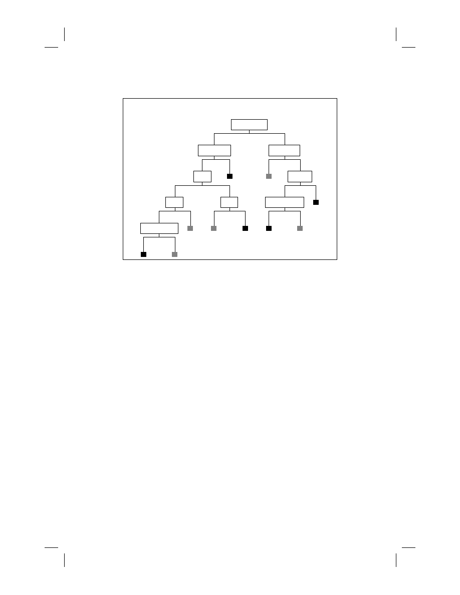
Figure 10.4

Red Terminal Node

= Above Average Response. Instances with a value

of the splitter greater than a threshold move to the right.

Note: The priors settings are unlike weights in that they do not affect the reported
counts in a node or the reported fractions of the sample in each target class. Priors do
affect the class any node is assigned to as well as the selection of the splitters in the
tree-growing process.

(Being able to rely on priors does not mean that the analyst should ignore the topic

of sampling at different rates from different target classes; rather, it gives the analyst
a broad range of ﬂexibility regarding when and how to sample.)

We used the “priors equal” settings to generate a CART tree for the mobile phone

data to better adapt to the relatively low probability of response and obtained the tree
schematic shown in Figure 10.4.

By convention, splits on continuous variables send instances with larger values

of the splitter to the right, and splits on nominal variables are deﬁned by the lists
of values going left or right. In the diagram the terminal nodes are color coded to
reﬂect the relative probability of response. A red node is above average in response
probability and a blue node is below average. Although this schematic displays only
a small fraction of the detailed reports available it is sufﬁcient to tell this fascinating
story: Even though they are quoted a high price for the new technology, households
with higher landline telephone bills who use a pager (beeper) service are more likely
to subscribe to the new service. The schematic also reveals how CART can reuse an

10.7 Missing Value Handling

189

attribute multiple times. Again, looking at the right side of the tree, and considering
households with larger landline telephone bills but without a pager service, we see
that the HANDPRIC attribute reappears, informing us that this customer segment is
willing to pay a somewhat higher price but will resist the highest prices. (The second
split on HANDPRIC is at 200.)

10.7

Missing Value Handling

Missing values appear frequently in the real world, especially in business-related
databases, and the need to deal with them is a vexing challenge for all modelers.
One of the major contributions of CART was to include a fully automated and ef-
fective mechanism for handling missing values. Decision trees require a missing
value-handling mechanism at three levels: (a) during splitter evaluation, (b) when
moving the training data through a node, and (c) when moving test data through a
node for ﬁnal class assignment. (See Quinlan, 1989 for a clear discussion of these
points.) Regarding (a), the ﬁrst version of CART evaluated each splitter strictly on its
performance on the subset of data for which the splitter is not missing. Later versions
of CART offer a family of penalties that reduce the improvement measure to reﬂect
the degree of missingness. (For example, if a variable is missing in 20% of the records
in a node then its improvement score for that node might be reduced by 20%, or alter-
natively by half of 20%, and so on.) For (b) and (c), the CART mechanism discovers
“surrogate” or substitute splitters for every node of the tree, whether missing values
occur in the training data or not. The surrogates are thus available, should a tree trained
on complete data be applied to new data that includes missing values. This is in sharp
contrast to machines that cannot tolerate missing values in the training data or that
can only learn about missing value handling from training data that include missing
values. Friedman (1975) suggests moving instances with missing splitter attributes
into both left and right child nodes and making a ﬁnal class assignment by taking a
weighted average of all nodes in which an instance appears. Quinlan opts for a variant
of Friedman’s approach in his study of alternative missing value-handling methods.
Our own assessments of the effectiveness of CART surrogate performance in the
presence of missing data are decidedly favorable, while Quinlan remains agnostic on
the basis of the approximate surrogates he implements for test purposes (Quinlan).
In Friedman, Kohavi, and Yun (1996), Friedman notes that 50% of the CART code
was devoted to missing value handling; it is thus unlikely that Quinlan’s experimental
version replicated the CART surrogate mechanism.

In CART the missing value handling mechanism is fully automatic and locally

adaptive at every node. At each node in the tree the chosen splitter induces a binary
partition of the data (e.g., X 1

<= c1 and X1 > c1). A surrogate splitter is a single

attribute Z that can predict this partition where the surrogate itself is in the form of
a binary splitter (e.g., Z

<= d and Z > d). In other words, every splitter becomes

a new target which is to be predicted with a single split binary tree. Surrogates are

190

CART: Classiﬁcation and Regression Trees

TABLE 10.3

Surrogate Splitter Report Main

Splitter TELEBILC Improvement

= 0.023722

Surrogate

Split

Association

Improvement

MARITAL

0.14

0.001864

TRAVTIME

2.5

0.11

0.006068

AGE

3.5

0.09

0.000412

CITY

2,3,5

0.07

0.004229

ranked by an association score that measures the advantage of the surrogate over the
default rule, predicting that all cases go to the larger child node (after adjustments
for priors). To qualify as a surrogate, the variable must outperform this default rule
(and thus it may not always be possible to ﬁnd surrogates). When a missing value is
encountered in a CART tree the instance is moved to the left or the right according
to the top-ranked surrogate. If this surrogate is also missing then the second-ranked
surrogate is used instead (and so on). If all surrogates are missing the default rule
assigns the instance to the larger child node (after adjusting for priors). Ties are broken
by moving an instance to the left.

Returning to the mobile phone example, consider the right child of the root node,

which is split on TELEBILC, the landline telephone bill. If the telephone bill data
are unavailable (e.g., the household is a new one and has limited history with the
company), CART searches for the attributes that can best predict whether the instance
belongs to the left or the right side of the split.

In this case (Table 10.3) we see that of all the attributes available the best predictor

of whether the landline telephone is high (greater than 50) is marital status (never-
married people spend less), followed by the travel time to work, age, and, ﬁnally, city
of residence. Surrogates can also be seen as akin to synonyms in that they help to
interpret a splitter. Here we see that those with lower telephone bills tend to be never
married, live closer to the city center, be younger, and be concentrated in three of the
ﬁve cities studied.

10.8

Attribute Importance

The importance of an attribute is based on the sum of the improvements in all nodes
in which the attribute appears as a splitter (weighted by the fraction of the training
data in each node split). Surrogates are also included in the importance calculations,
which means that even a variable that never splits a node may be assigned a large
importance score. This allows the variable importance rankings to reveal variable
masking and nonlinear correlation among the attributes. Importance scores may op-
tionally be conﬁned to splitters; comparing the splitters-only and the full (splitters
and surrogates) importance rankings is a useful diagnostic.

10.9 Dynamic Feature Construction

191

TABLE 10.4

Variable Importance (Including Surrogates)

Attribute

Score

TELEBILC

100.00

||||||||||||||||||||||||||||||||||||||||||

HANDPRIC

68.88

|||||||||||||||||||||||||||||

AGE

55.63

|||||||||||||||||||||||

CITY

39.93

||||||||||||||||

SEX

37.75

|||||||||||||||

PAGER

34.35

||||||||||||||

TRAVTIME

33.15

|||||||||||||

USEPRICE

17.89

|||||||

RENTHOUS

11.31

||||

MARITAL

6.98

TABLE 10.5

Variable Importance (Excluding Surrogates)

Variable

Score

TELEBILC

100.00

||||||||||||||||||||||||||||||||||||||||||

HANDPRIC

77.92

|||||||||||||||||||||||||||||||||

AGE

51.75

|||||||||||||||||||||

PAGER

22.50

|||||||||

CITY

18.09

|||||||

Observe that the attributes MARITAL, RENTHOUS, TRAVTIME, and SEX in

Table 10.4 do not appear as splitters but still appear to have a role in the tree. These
attributes have nonzero importance strictly because they appear as surrogates to the
other splitting variables. CART will also report importance scores ignoring the sur-
rogates on request. That version of the attribute importance ranking for the same tree
is shown in Table 10.5.

10.9

Dynamic Feature Construction

Friedman (1975) discusses the automatic construction of new features within each
node and, for the binary target, suggests adding the single feature

× w

where x is the subset of continuous predictor attributes vector and

w is a scaled dif-

ference of means vector across the two classes (the direction of the Fisher linear dis-
criminant). This is similar to running a logistic regression on all continuous attributes

192

CART: Classiﬁcation and Regression Trees

in the node and using the estimated logit as a predictor. In the CART monograph, the
authors discuss the automatic construction of linear combinations that include feature
selection; this capability has been available from the ﬁrst release of the CART soft-
ware. BFOS also present a method for constructing Boolean combinations of splitters
within each node, a capability that has not been included in the released software.
While there are situations in which linear combination splitters are the best way to
uncover structure in data (see Olshen’s work in Huang et al., 2004), for the most
part we have found that such splitters increase the risk of overﬁtting due to the large
amount of learning they represent in each node, thus leading to inferior models.

10.10

Cost-Sensitive Learning

Costs are central to statistical decision theory but cost-sensitive learning received
only modest attention before Domingos (1999). Since then, several conferences have
been devoted exclusively to this topic and a large number of research papers have
appeared in the subsequent scientiﬁc literature. It is therefore useful to note that
the CART monograph introduced two strategies for cost-sensitive learning and the
entire mathematical machinery describing CART is cast in terms of the costs of
misclassiﬁcation. The cost of misclassifying an instance of class i as class j is C(i

, j)

and is assumed to be equal to 1 unless speciﬁed otherwise; C(i

, i) = 0 for all i. The

complete set of costs is represented in the matrix C containing a row and a column
for each target class. Any classiﬁcation tree can have a total cost computed for its
terminal node assignments by summing costs over all misclassiﬁcations. The issue in
cost-sensitive learning is to induce a tree that takes the costs into account during its
growing and pruning phases.

The ﬁrst and most straightforward method for handling costs makes use of weight-

ing: Instances belonging to classes that are costly to misclassify are weighted upward,
with a common weight applying to all instances of a given class, a method recently
rediscovered by Ting (2002). As implemented in CART, weighting is accomplished
transparently so that all node counts are reported in their raw unweighted form. For
multiclass problems BFOS suggested that the entries in the misclassiﬁcation cost ma-
trix be summed across each row to obtain relative class weights that approximately
reﬂect costs. This technique ignores the detail within the matrix but has now been
widely adopted due to its simplicity. For the Gini splitting rule, the CART authors
show that it is possible to embed the entire cost matrix into the splitting rule, but only
after it has been symmetrized. The “symGini” splitting rule generates trees sensitive
to the difference in costs C(i

, j) and C(i, k), and is most useful when the symmetrized

cost matrix is an acceptable representation of the decision maker’s problem. By con-
trast, the instance weighting approach assigns a single cost to all misclassiﬁcations
of objects of class i . BFOS observe that pruning the tree using the full cost matrix is
essential to successful cost-sensitive learning.

10.11 Stopping Rules, Pruning, Tree Sequences, and Tree Selection

193

10.11

Stopping Rules, Pruning, Tree Sequences,
and Tree Selection

The earliest work on decision trees did not allow for pruning. Instead, trees were
grown until they encountered some stopping condition and the resulting tree was
considered ﬁnal. In the CART monograph the authors argued that no rule intended
to stop tree growth can guarantee that it will not miss important data structure
(e.g., consider the two-dimensional XOR problem). They therefore elected to grow
trees without stopping. The resulting overly large tree provides the raw material from
which a ﬁnal optimal model is extracted.

The pruning mechanism is based strictly on the training data and begins with a

cost-complexity measure deﬁned as

Ra(T )

= R(T ) + a|T |

where R(T ) is the training sample cost of the tree,

|T | is the number of terminal nodes

in the tree and a is a penalty imposed on each node. If a

= 0, then the minimum

cost-complexity tree is clearly the largest possible. If a is allowed to progressively
increase, the minimum cost-complexity tree will become smaller because the splits
at the bottom of the tree that reduce R(T ) the least will be cut away. The parameter
a is progressively increased in small steps from 0 to a value sufﬁcient to prune away
all splits. BFOS prove that any tree of size Q extracted in this way will exhibit
a cost R(Q) that is minimum within the class of all trees with Q terminal nodes.
This is practically important because it radically reduces the number of trees that
must be tested in the search for the optimal tree. Suppose a maximal tree has

|T |

terminal nodes. Pruning involves removing the split generating two terminal nodes
and absorbing the two children into their parent, thereby replacing the two terminal
nodes with one. The number of possible subtrees extractable from the maximal tree
by such pruning will depend on the speciﬁc topology of the tree in question but
will sometimes be greater than .5

|T |! But given cost-complexity pruning we need

to examine a much smaller number of trees. In our example we grew a tree with 81
terminal nodes and cost-complexity pruning extracts a sequence of 28 subtrees, but
if we had to look at all possible subtrees we might have to examine on the order of
25!

= 15,511,210,043,330,985,984,000,000 trees.

The optimal tree is deﬁned as that tree in the pruned sequence that achieves min-

imum cost on test data. Because test misclassiﬁcation cost measurement is subject
to sampling error, uncertainty always remains regarding which tree in the pruning
sequence is optimal. Indeed, an interesting characteristic of the error curve (misclas-
siﬁcation error rate as a function of tree size) is that it is often ﬂat around its minimum
for large training data sets. BFOS recommend selecting the “1 SE” tree that is the
smallest tree with an estimated cost within 1 standard error of the minimum cost (or
“0 SE”) tree. Their argument for the 1 SE rule is that in simulation studies it yields a
stable tree size across replications whereas the 0 SE tree size can vary substantially
across replications.

194

CART: Classiﬁcation and Regression Trees

Figure 10.5

One stage in the CART pruning process: the 17-terminal-node subtree.

Highlighted nodes are to be pruned next.

Figure 10.5 shows a CART tree along with highlighting of the split that is to be

removed next via cost-complexity pruning.

Table 10.6 contains one row for every pruned subtree obtained starting with the

maximal 81-terminal-node tree grown. The pruning sequence continues all the way
back to the root because we must allow for the possibility that our tree will demonstrate
no predictive power on test data. The best performing subtree on test data is the SE
0 tree with 40 nodes, and the smallest tree within a standard error of the SE 0 tree
is the SE 1 tree (with 35 terminal nodes). For simplicity we displayed details of the
suboptimal 10-terminal-node tree in the earlier dicussion.

10.12

Probability Trees

Probability trees have been recently discussed in a series of insightful articles elu-
cidating their properties and seeking to improve their performance (see Provost and
Domingos, 2000). The CART monograph includes what appears to be the ﬁrst detailed
discussion of probability trees and the CART software offers a dedicated splitting rule
for the growing of “class probability trees.” A key difference between classiﬁcation
trees and probability trees is that the latter want to keep splits that generate two termi-
nal node children assigned to the same class as their parent whereas the former will
not. (Such a split accomplishes nothing so far as classiﬁcation accuracy is concerned.)
A probability tree will also be pruned differently from its counterpart classiﬁcation
tree. Therefore, building both a classiﬁcation and a probability tree on the same data in
CART will yield two trees whose ﬁnal structure can be somewhat different (although
the differences are usually modest). The primary drawback of probability trees is that
the probability estimates based on training data in the terminal nodes tend to be biased
(e.g., toward 0 or 1 in the case of the binary target) with the bias increasing with the
depth of the node. In the recent ML literature the use of the Laplace adjustment has
been recommended to reduce this bias (Provost and Domingos, 2002). The CART
monograph offers a somewhat more complex method to adjust the terminal node

10.12 Probability Trees

195

TABLE 10.6

Complete Tree Sequence for CART Model: All Nested Subtrees

Reported

Tree

Nodes

Test Cost

Train Cost

Complexity

0.635461

+/-

0.046451

0.197939

0.646239

+/-

0.046608

0.200442

0.000438

0.640309

+/-

0.046406

0.210385

0.00072

0.638889

+/-

0.046395

0.217487

0.000898

0.632373

+/-

0.046249

0.219494

0.001013

0.635214

+/-

0.046271

0.23194

0.001255

0.643151

+/-

0.046427

0.242131

0.001284

0.639475

+/-

0.046303

0.262017

0.00143

0.592442

+/-

0.044947

0.289254

0.001709

0.584506

+/-

0.044696

0.296356

0.001786

0.611156

+/-

0.045432

0.317663

0.002141

0.633049

+/-

0.045407

0.331868

0.002377

0.635891

+/-

0.045425

0.336963

0.002558

0.638731

+/-

0.045442

0.342307

0.002682

0.674738

+/-

0.046296

0.347989

0.002851

0.677918

+/-

0.045841

0.374143

0.003279

0.659204

+/-

0.045366

0.381245

0.003561

0.648764

+/-

0.044401

0.431548

0.003603

0.692798

+/-

0.044574

0.442911

0.005692

0.725379

+/-

0.04585

0.455695

0.006402

0.756539

+/-

0.046819

0.486269

0.007653

0.785534

+/-

0.046752

0.53975

0.008924

0.784542

+/-

0.045015

0.563898

0.012084

0.784542

+/-

0.045015

0.620536

0.014169

0.784542

+/-

0.045015

0.650253

0.014868

0.784542

+/-

0.045015

0.71043

0.015054

0.907265

+/-

0.047939

0.771329

0.015235

+/-

0.114345

estimates that has rarely been discussed in the literature. Dubbed the “Breiman ad-
justment,” it adjusts the estimated misclassiﬁcation rate r

× (t) of any terminal node

upward by

× (t) = r(t) + e/(q(t) + S)

where r (t) is the training sample estimate within the node, q(t) is the fraction of
the training sample in the node, and S and e are parameters that are solved for as a
function of the difference between the train and test error rates for a given tree. In
contrast to the Laplace method, the Breiman adjustment does not depend on the raw
predicted probability in the node and the adjustment can be very small if the test data
show that the tree is not overﬁt. Bloch, Olshen, and Walker (2002) discuss this topic
in detail and report very good performance for the Breiman adjustment in a series of
empirical experiments.

196

CART: Classiﬁcation and Regression Trees

10.13

Theoretical Foundations

The earliest work on decision trees was entirely atheoretical. Trees were proposed as
methods that appeared to be useful and conclusions regarding their properties were
based on observing tree performance on empirical examples. While this approach
remains popular in machine learning, the recent tendency in the discipline has been
to reach for stronger theoretical foundations. The CART monograph tackles theory
with sophistication, offering important technical insights and proofs for key results.
For example, the authors derive the expected misclassiﬁcation rate for the maximal
(largest possible) tree, showing that it is bounded from above by twice the Bayes
rate. The authors also discuss the bias variance trade-off in trees and show how
the bias is affected by the number of attributes. Based largely on the prior work of
CART coauthors Richard Olshen and Charles Stone, the ﬁnal three chapters of the
monograph relate CART to theoretical work on nearest neighbors and show that as
the sample size tends to inﬁnity the following hold: (1) the estimates of the regression
function converge to the true function and (2) the risks of the terminal nodes converge
to the risks of the corresponding Bayes rules. In other words, speaking informally,
with large enough samples the CART tree will converge to the true function relating
the target to its predictors and achieve the smallest cost possible (the Bayes rate).
Practically speaking, such results may only be realized with sample sizes far larger
than in common use today.

10.14

Post-CART Related Research

Research in decision trees has continued energetically since the 1984 publication of
the CART monograph, as shown in part by the several thousand citations to the mono-
graph found in the scientiﬁc literature. For the sake of brevity we conﬁne ourselves
here to selected research conducted by the four CART coauthors themselves after
1984. In 1985 Breiman and Friedman offered ACE (alternating conditional expecta-
tions), a purely data-based driven methodology for suggesting variable transforma-
tions in regression; this work strongly inﬂuenced Hastie and Tibshirani’s generalized
additive models (GAM, 1986). Stone (1985) developed a rigorous theory for the style
of nonparametric additive regression proposed with ACE. This was soon followed by
Friedman’s recursive partitioning approach to spline regression (multivariate adaptive
regression splines, MARS). The ﬁrst version of the MARS program in our archives
is labeled Version 2.5 and dated October 1989; the ﬁrst published paper appeared as
a lead article with discussion in the Annals of Statistics in 1991. The MARS algo-
rithm leans heavily on ideas developed in the CART monograph but produces models

10.14 Post-CART Related Research

197

that are readily recognized as regressions on recursively partitioned (and selected)
predictors. Stone, with collaborators, extended the spline regression approach to haz-
ard modeling (Kooperberg, Stone, and Truong, 1995) and polychotomous regression
(1997).

Breiman was active in searching for ways to improve the accuracy, scope of ap-

plicability, and compute speed of the CART tree. In 1992 Breiman was the ﬁrst to
introduce the multivariate decision tree (vector dependent variable) in software but
did not write any papers on the topic. In 1995, Spector and Breiman implemented
a strategy for parallelizing CART across a network of computers using the C-Linda
parallel programming environment. In this study the authors observed that the gains
from parallelization were primarily achieved for larger data sets using only a few
of the available processors. By 1994 Breiman had hit upon “bootstrap aggregation”:
creating predictive ensembles by growing a large number of CART trees on boot-
strap samples drawn from a ﬁxed training data set. In 1998 Breiman applied the idea
of ensembles to online learning and the development of classiﬁers for very large
databases. He then extended the notion of randomly sampling rows in the training
data to random sampling columns in each node of the tree to arrive at the idea of
the random forest. Breiman devoted the last years of his life to extending random
forests with his coauthor Adele Cutler, introducing new methods for missing value
imputation, outlier detection, cluster discovery, and innovative ways to visualize data
using random forests outputs in a series of papers and Web postings from 2000
to 2004.

Richard Olshen has focused primarily on biomedical applications of decision trees.

He developed the ﬁrst tree-based approach to survival analysis (Gordon and Olshen,
1984), contributed to research on image compression (Cosman et al., 1993), and has
recently introduced new linear combination splitters for the analysis of very high
dimensional data (the genetics of complex disease).

Friedman introduced stochastic gradient boosting in several papers beginning in

1999 (commercialized as TreeNet software) which appears to be a substantial ad-
vance over conventional boosting. Friedman’s approach combines the generation of
very small trees, random sampling from the training data at every training cycle,
slow learning via very small model updates at each training cycle, selective rejection
of training data based on model residuals, and allowing for a variety of objective
functions, to arrive at a system that has performed remarkably well in a range of real-
world applications. Friedman followed this work with a technique for compressing
tree ensembles into models containing considerably fewer trees using novel methods
for regularized regression. Friedman showed that postprocessing of tree ensembles to
compress them may actually improve their performance on holdout data. Taking this
line of research one step further, Friedman then introduced methods for reexpressing
tree ensemble models as collections of “rules” that can also radically compress the
models and sometimes improve their predictive accuracy.

Further pointers to the literature, including a library of applications of CART, can

be found at the Salford Systems Web site: http://www.salford-systems.com.

198

CART: Classiﬁcation and Regression Trees

10.15

Software Availability

CART software is available from Salford Systems, at http://www.salford-
systems.com; no-cost evaluation versions may be downloaded on request. Executables
for Windows operating systems as well as Linux and UNIX may be obtained in
both 32-bit and 64-bit versions. Academic licenses for professors automatically grant
no-cost licenses to their registered students. CART source code, written by Jerome
Friedman, has remained a trade secret and is available only in compiled binaries
from Salford Systems. While popular open-source systems (and other commercial
proprietary systems) offer decision trees inspired by the work of Breiman, Friedman,
Olshen, and Stone, these systems generate trees that are demonstrably different from
those of true CART when applied to real-world complex data sets. CART has been
used by Salford Systems to win a number of international data mining competitions;
details are available on the company’s Web site.

10.16

Exercises

1. (a) To the decision tree novice the most important variable in a CART tree should

be the root node splitter, yet it is not uncommon to see a different variable listed
as most important in the CART summary output. How can this be? (b) If you
run a CART model for the purpose of ranking the predictor variables in your
data set and then you rerun the model excluding all the 0-importance variables,
will you get the same tree in the second run? (c) What if you rerun the tree
keeping as predictors only variables that appeared as splitters in the ﬁrst run?
Are there conditions that would guarantee that you obtain the same tree?

2. Every internal node in a CART tree contains a primary splitter, competitor

splits, and surrogate splits. In some trees the same variable will appear as both
a competitor and a surrogate but using different split points. For example, as a
competitor the variable might split the node with x j

<= c, while as a surrogate

the variable might split the node as x j

<= d. Explain why this might occur.

3. Among its six different splitting rules CART offers the Gini and twoing splitting

rules for growing a tree. Explain why an analyst might prefer the results of the
twoing rule even if it yielded a lower accuracy.

4. For a binary target if two CART trees are grown on the same data, the ﬁrst

using the Gini splitting rule and the second using the class probability rule,
which one is likely to contain more nodes? Will the two trees exhibit the same
accuracy? Will the smaller tree be contained within the larger one? Explain the
differences between the two trees.

5. Suppose you have a data set for a binary target coded 0/1 in which 80% of the

records have a target value of 0 and you grow a CART tree using the default

References

199

PRIORS EQUAL setting. How will the results change if you rerun the model
using a WEIGHT variable

w with w = 1 when the target is 0 and w = 4 when

the target is 1?

6. When growing CART trees on larger data sets containing tens of thousands of

records or more, one often ﬁnds that tree accuracy declines only slightly as the
tree is grown much larger than its optimal size. In other words, on large data
sets a too-large CART tree appears to overﬁt only slightly. Why is this the case?

7. A CART model is not just a single tree but a collection of nested trees, each of

which has its own performance characteristics (accuracy, area under the ROC
curve). Why do the CART authors suggest that the best tree is not necessarily
the most accurate tree but could well be the smallest tree in the tree sequence
within some tolerance interval of the most accurate tree? How is the tolerance
interval calculated?

8. For cost-sensitive learning, when different mistakes are associated with differ-

ent costs, the CART authors adjust the priors to reﬂect costs, which is essentially
a form of reweighting the data. When do adjusted priors perfectly reﬂect costs
and when do they only approximate the costs? How does the symmetric gini
splitting rule help to reﬂect costs of misclassiﬁcation?

9. The CART authors decided on a grow-then-prune strategy for the selection of an

optimal decision tree rather than following an apparently simpler stopping rule
method. Explain how XOR-type problems can be used to defeat any stopping
rule based on a goodness of split criterion for one or more splits.

10. If a training data set is complete (contains no missing values in any predictor),

how can a CART tree grown on such data guarantee that it can handle missing
values encountered in future data?

References

Bloch, D.A., Olshen, R.A., and Walker M.G. (2002) Risk estimation for classiﬁcation

trees. Journal of Computational & Graphical Statistics, 11, 263–288.

Breiman, L. (1995) Current research in the mathematics of generalization. Proceed-

ings of the Santa Fe Institute CNLS Workshop on Formal Approaches to Supervised
Learning. David Wolpert, Ed. Addison-Wesley, 361–368.

Breiman, L. (1998) Pasting Small Votes for Classiﬁcation in Large Databases and

On-Line. Statistics Department, University of California, Berkeley.

Breiman, L., and Friedman, J.H. (1985) Estimating optimal transformations for mul-

tiple regression and correlation. Journal of the American Statistical Association,
80, 580–598.

200

CART: Classiﬁcation and Regression Trees

Breiman, L., Friedman, J.H., Olshen, R.A., and Stone, C.J. (1984) Classiﬁcation and

Regression Trees, Wadsworth, Belmont, CA. Republished by CRC Press.

Breiman, L. and Stone, J. (1978) Parsimonious Binary Classiﬁcation Trees, Technical

Report, Technology Services Corp., Los Angeles.

Cosman, P.C., Tseng, C., Gray, R.M., Olshen, R.A., et al. (1993) Tree-structured

vector quantization of CT chest scans: Image quality and diagnostic accuracy.
IEEE Transactions on Medical Imaging, 12, 727–739.

Cover, T. and Hart, P. (1967) Nearest neighbor pattern classiﬁcation, IEEE Trans

Information Theory 13, page(s): 21–27.

Domingos, P. (1999) MetaCost: A general method for making classiﬁers cost-

sensitive. In Proceedings of the Fifth International Conference on Knowledge Dis-
covery and Data Mining, pp. 155–164.

Doyle, P. (1973) The use of automatic interaction detector and similar search proce-

dures. Operational Research Quarterly, 24, 465–467.

Einhorn, H. (1972) Alchemy in the behavioral sciences. Public Opinion Quarterly,

36, 367–378.

Friedman, J.H. (1977) A recursive partitioning decision rule for nonparametric clas-

siﬁcation. IEEE Trans. Computers, C-26, 404. Also available as Stanford Linear
Accelerator Center Rep. SLAC-PUB-1373 (Rev. 1975).

Friedman, J.H. (1999) Stochastic Gradient Boosting. Statistics Department, Stanford

University.

Friedman, J.H., Bentley, J.L., and Finkel, R.A. (1977) An algorithm for ﬁnding best

matches in logarithmic time. ACM Trans. Math. Software, 3, 209. Also available
as Stanford Linear Accelerator Center Rep. SIX-PUB-1549, Feb. 1975.

Friedman, J.H., Kohavi, R., and Yun, Y. (1996) Lazy decision trees. In Proceedings of

the Thirteenth National Conference on Artiﬁcial Intelligence, pp. 717–724, AAAI
Press/MIT Press, San Francisco, CA.

Gordon, L., and Olshen, R.A. (1985) Tree-structured survival analysis (with discus-

sion). Cancer Treatment Reports, 69, 1065–1068.

Gordon, L., and Olshen, R.A. (1984) Almost surely consistent nonparametric regres-

sion from recursive partitioning schemes. Journal of Multivariate Analysis, 15,
147–163.

Hastie and Tibshirani’s Generalized Additive Models. (1986) Statistical Science. 1,

297–318.

Huang, J., Lin, A., Narasimhan, B., et al. (2004) Tree-structured supervised learning

and the genetics of hypertension. Proc. Natl. Acad. Sci., July 20, 101(29), 10529–
10534.

References

201

Kooperberg, C., Bose, S., and Stone, C.J. (1997) Polychotomous regression. Journal

of the American Statistical Association, 92, 117–127.

Kooperberg, C., Stone, C.J., and Truong, Y.K. (1995) Hazard regression. Journal of

the American Statistical Association, 90, 78–94.

Messenger, R.C., and Mandell, M.L. (1972) A model search technique for predictive

nominal scale multivariate analysis. Journal of the American Statistical Associa-
tion, 67, 768–772.

Morgan, J.N., and Sonquist, J.A. (1963) Problems in the analysis of survey data, and

a proposal. Journal of the American Statistical Association, 58, 415–435.

Provost, F., and Domingos, P. (2002) Tree induction for probability-based ranking.

Machine Learning, 52, 199–215.

Quinlan, R. (1989) Unknown attribute values in induction. In Proceedings of the Sixth

International Workshop on Machine Learning, pp. 164–168.

Stone, C.J. (1977) Consistent nonparametric regression (with discussion). Annals of

Statistics, 5, 595–645.

Stone, C. (1985) Additive regression and other non-parametric models, Annal. Statist.,

13, 689–705.

Ting, K.M. (2002) An instance-weighting method to induce cost-sensitive trees. IEEE

Trans. Knowledge and Data Engineering, 14, 659–665.

Document Outline

The Top Ten Algorithms in Data Mining
- Table of Contents
- Chapter 10: CART: Classification and Regression Trees

Wyszukiwarka

Podobne podstrony:
DK3171 C010
c9641 c005
c9641 c008

więcej podobnych podstron

c9641 c010

Document Outline