
Complex Analysis 2002-2003
c
K. Houston 2003
1
Complex Functions
In this section we will define what we mean by a complex func-
tion. We will then generalise the definitions of the exponential,
sine and cosine functions using complex power series. To deal
with complex power series we define the notions of conver-
gent and absolutely convergent, and see how to use the ratio
test from real analysis to determine convergence and radius
of convergence for these complex series.
We start by defining domains in the complex plane. This
requires the prelimary definition.
Definition 1.1
The ε-neighbourhood of a complex number z is the set of com-
plex numbers {w ∈ C : |z − w| < ε} where ε is positive number.
Thus the ε-neigbourhood of a point z is just the set of points
lying within the circle of radius ε centred at z. Note that it
doesn’t contain the circle.
Definition 1.2
A domain is a non-empty subset D of C such that for every
point in D there exists a ε-neighbourhood contained in D.
Examples 1.3
The following are domains.
(i) D = C. (Take c ∈ C. Then, any ε > 0 will do for an ε-
neighbourhood of c.)
(ii) D = C\{0}. (Take c ∈ D and let ε =
1
2
(|c|)
. This gives a
ε
-neighbourhood of c in D.)
(iii) D = {z : |z − a| < R} for some R > 0. (Take c ∈ C and let
ε =
1
2
(R − |c − a|)
. This gives a ε-neighbourhood of c in D.)
Example 1.4
The set of real numbers R is not a domain. Consider any
real number, then any ε-neighbourhood must contain some
complex numbers, i.e. the ε-neighbourhood does not lie in the
real numbers.
We can now define the basic object of study.
1

Definition 1.5
Let D be a domain in C. A complex function, denoted f : D →
C, is a map which assigns to each z in D an element of C, this
value is denoted f (z).
Common Error 1.6
Note that f is the function and f (z) is the value of the function
at z. It is wrong to say f (z) is a function, but sometimes people
do.
Examples 1.7
(i) Let f (z) = z
2
for all z ∈ C.
(ii) Let f (z) = |z| for all z ∈ C. Note that here we have a
complex function for which every value is real.
(iii) Let f (z) = 3z
4
− (5 − 2i)z
2
+ z − 7
for all z ∈ C. All complex
polynomials give complex functions.
(iv) Let f (z) = 1/z for all z ∈ C\{0}. This function cannot be
extended to all of C.
Remark 1.8
Functions such as sin x for x real are not complex functions
since the real line in C is not a domain. Later we see how to
extend the concept of the sine so that it is complex function
on the whole of the complex plane.
Obviously, if f and g are complex functions, then f + g,
f − g
, and f g are functions given by (f + g)(z) = f (z) + g(z),
(f − g)(z) = f (z) − g(z)
, and (f g)(z) = f (z)g(z), respectively.
We can also define (f /g)(z) = f (z)/g(z) provided that g(z) 6= 0
on D. Thus we can build up lots of new functions by these
elementary operations.
The aim of complex analysis
We wish to study complex functions. Can we define differenti-
ation? Can we integrate? Which theorems from Real Analysis
can be extended to complex analysis? For example, is there a
version of the mean value theorem? Complex analysis is es-
sentially the attempt to answer these questions. The theory
will be built upon real analysis but in many ways it is easier
than real analysis. For example if a complex function is dif-
ferentiable (defined later), then its derivative is also differen-
tiable. This is not true for real functions. (Do you know an ex-
ample of a differentiable real function with non-differentiable
derivative?)
2

Real and imaginary parts of functions
We will often use z to denote a complex number and we will
have z = x + iy where x and y are both real. The value f (z)
is a complex number and so has a real and imaginary part.
We often use u to denote the real part and v to denote the
imaginary part. Note that u and v are functions of z.
We often write f (x + iy) = u(x, y) + iv(x, y). Note that u is
a function of two real variables, x and y. I.e. u : R
2
→ R.
Similarly for v.
Examples 1.9
(i) Let f (z) = z
2
. Then, f (x + iy) = (x + iy)
2
= x
2
− y
2
+ 2ixy
. So,
u(x, y) = x
2
− y
2
and v(x, y) = xy.
(ii) Let f (z) = |z|. Then, f (x + iy) =
px
2
+ y
2
. So, u(x, y) =
px
2
+ y
2
and v(x, y) = 0.
Exercises 1.10
Find u and v for the following:
(i) f (z) = 1/z for z ∈ C\{0}.
(ii) f (z) = z
3
.
Visualising complex functions
In Real Analysis we could draw the graph of a function. We
have an axis for the variable and an axis for the value, and so
we can draw the graph of the function on a piece of paper.
For complex functions we have a complex variable (that’s
two real variables) and the value (another two real variables),
so if we want to draw a graph we will need 2 + 2 = 4 real
variables, i.e. we will have to work in 4-dimensional space.
Now obviously this is a bit tricky because we are used to 3
space dimensions and find visualising 4 dimensional space
very hard.
Thus, it is very difficult to visualise complex functions. How-
ever, there are some methods available:
(i) We can draw two complex planes, one for the domain and
one for the range.
3

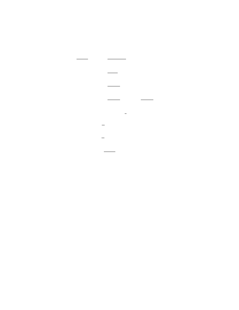
(ii) The two-variable functions u and v can be visualised sep-
arately. The graph of a function of two variables is a sur-
face in three space.
u(x, y) = cos x + sin y
and v(x, y) = x
2
− y
2
(iii) Make one of the variables time and view the graph as
something that evolves over time. This is not very helpful.
Defining e
z
, cos z and sin z
First we will try and define some elementary complex func-
tions to play with. How shall we define functions such as e
z
,
cos z
and sin z? We require that their definition should coincide
with the real version when z is a real number, and we would
like them to have properties similar to the real versions of the
functions, e.g. sin
2
z + cos
2
z = 1
would be nice. However, sine
and cosine are defined using trigonometry and so are hard to
generalise: for example, what does it mean for a triangle to
have an hypotenuse of length 2 + 3i? The exponential is de-
fined using differential calculus and we have not yet defined
differentiation of complex functions.
However, we know from Real Analysis that the functions
can be described using a power series, e.g.,
sin x = x −
x
3
3!
+
x
5
5!
− · · · =
∞
X
n=0
(−1)
n
x
2n+1
(2n + 1)!
.
Thus, for z ∈ C, we shall define the exponential, sine and
cosine of z as follows:
e
z
:=
∞
X
n=0
z
n
n!
,
sin z :=
∞
X
n=0
(−1)
n
z
2n+1
(2n + 1)!
,
cos z :=
∞
X
n=0
(−1)
n
z
2n
(2n)!
.
4
Thus,
e
3+2i
=
∞
X
n=0
(3 + 2i)
n
n!
= 1 + (3 + 2i) +
(3 + 2i)
2
2!
+
(3 + 2i)
3
3!
+ . . .
These definitions obviously satisfy the requirement that they
coincide with the definitions we know and love for real z, but
how can we be sure that the series converges? I.e. when we
put in a z, such as 3 + 2i, into the definition, does a complex
number comes out?
To answer this we will have to study complex series and
as the theory of real series was built on the theory of real
sequences
we had better start with complex sequences.
Complex Sequences
The definition of convergence of a complex sequence is the
same as that for convergence of a real sequence.
Definition 1.11
A complex sequence hc
n
i converges to c ∈ C, if given any ε > 0,
then there exists N such that |c
n
− c| < ε for all n ≥ N .
We write c
n
→ c or lim
n→∞
c
n
= c
.
Example 1.12
The sequence c
n
=
4 − 3i
7
n
converges to zero.
Consider
|c
n
− 0| = |c
n
| =
4 − 3i
7
n
=
4 − 3i
7
n
=
r
25
49
!
n
=
5
7
n
.
So
|c
n
− 0| < ε
⇐⇒
(5/7)
n
< ε
⇐⇒
n log(5/7) < log ε
⇐⇒
n >
log ε
log(5/7)
.
So, given any ε we can choose N to be any natural number
greater than log ε/ log(5/7). Thus the sequence converges to
zero.
Remark 1.13
Notice that a
n
= |c
n
− c| is a real sequence, and that c
n
→ c if
and only if the real sequence |c
n
− c| → 0. Hence, we are saying
something about a complex sequence using real analysis.
5

Paradigm 1.14
The remark above gives a good example of the paradigm
1
we
will be using. We can apply results from real analysis to pro-
duce results in complex analysis. In this case we take the
modulus, but we can also take real and imaginary parts.
This is a key observation. Note it well!
Let’s apply the paradigm. The next proposition shows that
a sequence converges if and only its real and imaginary parts
do.
Proposition 1.15
Let c
n
= a
n
+ ib
n
where a
n
and b
n
are real sequences, and c =
a + ib
. Then
c
n
→ c ⇐⇒ a
n
→ a and b
n
→ b.
Proof. [⇒] If c
n
→ c, then |c
n
− c| → 0. But
0 ≤ |a
n
− a| = |Re(c
n
) − Re(c)| = |Re(c
n
− c)| ≤ |c
n
− c|.
So by the squeeze rule |a
n
− a| → 0, i.e. a
n
→ a. Similarly,
b
n
→ b.
[⇐] Suppose a
n
→ a and b
n
→ b, then |a
n
− a| → 0, and
|b
n
− b| → 0. We have
0 ≤ |c
n
− c| = |(a
n
− a) + i(b
n
− b)| ≤ |a
n
− a| + |b
n
− b|.
The last inequality follows from the triangle inequality applied
to z = a
n
−a and w = i(b
n
−b). Because |a
n
−a| → 0 and |b
n
−b| → 0
we deduce |c
n
− c| → 0, i.e. c
n
→ c.
HTTLAM 1.16
Try not to use the definition of convergence to prove that a
sequence converges.
Example 1.17
n
2
+ in
3
n
3
+ 1
=
n
2
n
3
+ 1
+ i
n
3
n
3
+ 1
→ 0 + i.1 = i.
Exercises 1.18
(i) Which of the following sequences converge(s)?
(n + 1)
5
n
5
i
and
5 − 12i
6
n
.
(ii) Show that the limit of a complex sequence is unique.
1
Paradigm: a conceptual model underlying the theories and practice of a scientific subject.
(Oxford English Dictionary).
6

Complex Series
Now that we have defined convergence of complex sequences
we can define convergence of complex series.
Definition 1.19
A complex series
P
∞
k=0
w
k
converges
if and only if the sequence
hs
n
i formed by its partial sums s
n
=
P
n
k=0
w
k
converges.
That is, the following sequences converges
s
0
= w
0
s
1
= w
0
+ w
1
s
2
= w
0
+ w
1
+ w
2
s
3
= w
0
+ w
1
+ w
2
+ w
3
..
.
Let’s apply the paradigm and give a result on complex series
using real series.
Proposition 1.20
Let w
k
= x
k
+ iy
k
where x
k
and y
k
are real for all k. Then,
∞
X
k=0
w
k
converges ⇐⇒
∞
X
k=0
x
k
and
∞
X
k=0
y
k
converge.
In this case
∞
X
k=0
w
k
=
∞
X
k=0
x
k
+ i
∞
X
k=0
y
k
.
Proof. Let a
n
=
P
n
k=0
x
k
, b
n
=
P
n
k=0
y
k
, and s
n
=
P
n
k=0
w
k
, and
apply Proposition 1.15.
The second part of the statement
comes from equating real and imaginary parts.
Example 1.21
The series
P
∞
n=0
(−1)
n
i
n!
converges. Let x
k
= 0
and y
k
=
(−1)
k
k!
.
Then
P x
k
= 0
, obviously, and
P
(−1)
k
k!
= e
−1
.
Thus
P
∞
n=0
(−1)
n
i
n!
converges to i/e.
In real analysis we have some great ways to tell if a series
is convergent, for example, the ratio test and the integral test.
Can we use the real analysis tests in complex analysis? The
next theorem says we can, but first let us make a definition.
Definition 1.22
We say
P
∞
k=0
w
k
is absolutely convergent if the real series
P
∞
k=0
|w
k
| converges.
7

This definition is really the same as in Real Analysis, it has
merely been extended to complex numbers in a natural way.
Now for a very important theorem which says that if a series
is absolutely convergent, then it is convergent.
Theorem 1.23
If
P
∞
k=0
|w
k
| converges, then
P
∞
k=0
w
k
converges.
This is a fantastic tool. Remember it. The assumption says
something about a real series (we know lots about these!) and
gives a conclusion about a complex series. Thus, we can apply
the ratio test or comparison test to the real series and say
something about the complex series. Great!
Proof. Let w
k
= x
k
+ iy
k
, with x
k
and y
k
real. Then
P
∞
k=0
|w
k
|
convergent implies that
P
∞
k=0
|x
k
| is convergent (because 0 ≤
|x
k
| = |Re(w
k
)| ≤ |w
k
| and we can apply the comparison test).
So the real series
P
∞
k=0
x
k
converges absolutely and we know
from Real Analysis I that this implies that
P
∞
k=0
x
k
converges.
Similarly, the series
P
∞
k=0
y
k
converges.
Then,
P
∞
k=0
w
k
=
P
∞
k=0
x
k
+ i
P
∞
k=0
y
k
, by Proposition 1.20.
HTTLAM 1.24
When asked to show a series converges, show it absolutely
converges.
Remark 1.25
Note that the converse to Theorem 1.23 is not true. We al-
ready know this from Real Analysis. For example,
P
∞
k=0
(−1)
k
k
converges but
P
∞
k=0
(−1)
k
k
=
P
∞
k=0
1
k
diverges.
We now prove an infinite version of the triangle inequality.
Lemma 1.26
Suppose that
P
∞
k=0
w
k
converges absolutely. Then
∞
X
k=0
w
k
≤
∞
X
k=0
|w
k
|.
Proof. For n ≥ 1,
∞
X
k=0
w
k
=
∞
X
k=0
w
k
−
n
X
k=0
w
k
+
n
X
k=0
w
k
≤
∞
X
k=0
w
k
−
n
X
k=0
w
k
+
n
X
k=0
w
k
≤
∞
X
k=0
w
k
−
n
X
k=0
w
k
+
n
X
k=0
|w
k
| .
8

As n → ∞ then obviously, |
P
∞
k=0
w
k
−
P
n
k=0
w
k
| → 0, hence the
result.
Definition 1.27
A complex power series is a sum of the form
P
m
k=0
c
k
z
k
, where
c
k
∈ C and m is possibly infinite.
Such a power series is a function of z. Much of the theory of
differentiable complex functions is concerned with power se-
ries, because as we shall see later, any differentiable complex
function can be represented as a power series.
Radius of Convergence
Just as with real power series we can have complex power
series that do not converge on the whole of the complex plane.
Example 1.28
Consider the series
P
∞
0
z
n
, where z ∈ C. We know for z = 1
this series does not converge because then we have
P
∞
0
1
n
=
P
∞
0
1 = 1 + 1 + 1 + . . .
.
We also know it converges for z = 0, because
P
∞
0
0
n
=
P
∞
0
0 = 0 + 0 + 0 + · · · = 0
. Hopefully, you remember from
Real Analysis I that for real z the power series converges only
for −1 < z < 1.
So, for which complex values of z does it converge? Let us
use the ratio test. Let a
n
= |z
n
|. Then
a
n+1
a
n
=
|z
n+1
|
|z
n
|
= |z|.
As n → ∞ we have |z| → |z|, because there is no dependence
on n. So by the ratio test the series
P a
n
converges if |z| < 1,
diverges if |z| > 1 and for |z| = 1 we don’t know what will
happen. So
P z
n
converges absolutely, and hence converges,
for |z| < 1.
That the set of complex numbers for which the series con-
verges is given by something of the form |z| < R for some R is
a general phenomenon, as the next theorem shows.
Theorem 1.29
Let
P
∞
0
a
n
z
n
be some complex power series. Then, there exists
R
, with 0 ≤ R ≤ ∞, such that
∞
X
0
a
n
z
n
converges absolutely for |z| < R,
diverges for |z| > R.
9
Proof. The proof is similar to that for real power series used
in Real Analysis I. Stewart and Tall also have a good proof, see
p56-57.
HTTLAM 1.30
Given a power series, immediately ask ‘What is its radius of
convergence?’
Exercise 1.31
Show that
P
∞
0
z
n
/n
has radius of convergence 1.
In the last exercise note that for z = −1 the series converges,
but for z = 1 the series diverges, (both these fact should be
well known from Real Analysis). This tells us that for |z| = 1
we can get some values of z for which the series converges and
some for which the series diverges.
Sine, cosine, and exponential are defined for all complex
numbers
Let us now return to showing that the sine, cosine and expo-
nential functions are defined on the whole of C.
Example 1.32
(I’ll do this example in great detail. The next example will be
more like the solution I would expect from you.)
The series e
z
=
P
∞
n=0
z
n
n!
converges for all z ∈ C.
For any z ∈ C let a
n
=
z
n
n!
. We want
P
∞
n=0
a
n
to converge, so
we use the ratio test on this real series. We have
a
n+1
a
n
=
z
n+1
(n + 1)!
z
n
n!
=
z
n+1
z
n
n!
(n + 1)!
=
|z|
n + 1
→ 0 as n → ∞.
The last part is true because for fixed z the real number |z| is
of course a finite constant.
So by the ratio test
P
∞
n=0
a
n
=
P
∞
n=0
z
n
n!
converges. Thus by
Theorem 1.23 the series
P
∞
n=0
z
n
n!
converges for all z ∈ C.
The following is an example with some of the small detail
missing. This is how I would expect the solution to be given if
I had set this as an exercise.
10
Example 1.33
The series sin z =
∞
X
n=0
(−1)
n
z
2n+1
(2n + 1)!
converges for all z ∈ C.
Let a
n
=
(−1)
n
z
2n+1
(2n + 1)!
. Then
a
n+1
a
n
=
z
2(n+1)+1
(2(n + 1) + 1)!
z
2n+1
(2n + 1)!
=
z
2n+3
(2n + 3)!
z
2n+1
(2n + 1)!
=
z
2
(2n + 3)(2n + 2)
=
|z|
2
(2n + 3)(2n + 2)
→ 0 as n → ∞.
So by the ratio test the complex series converges absolutely,
and hence converges.
Exercise 1.34
Prove that cos z converges for all z.
Properties of the exponential
We have defined the exponential function and shown that is
defined on all of C, let’s now look at its properties. Most of
these you may already from Numbers and Proofs, but the
proofs may not have been rigorous.
Theorem 1.35
(i) e
¯
z
= e
z
, for all z ∈ C.
(ii) e
iz
= cos z + i sin z
, for all z ∈ C.
(iii) e
z+w
= e
z
e
w
, for all z, w ∈ C.
(iv) e
z
6= 0, for all z ∈ C.
(v) e
−z
= 1/e
z
, for all z ∈ C.
(vi) e
nz
= (e
z
)
n
, for all z ∈ C and n ∈ Z.
(vii) |e
z
| = e
Re(z)
, for all z ∈ C.
(viii) |e
iy
| = 1, for all y ∈ R.
Proof. (i) We have
e
¯
z
=
∞
X
n=0
(¯
z)
n
n!
=
∞
X
n=0
(z
n
)
n!
=
∞
X
n=0
z
n
n!
= e
z
.
11

(ii) Exercise. (Just put iz into the power series and separate
the real and imaginary parts.)
(iii) This will be delayed until we deal with differentiability.
(iv) Note that e
z
and e
−z
both exist. We have
e
z
e
−z
= e
z−z
by (iii),
= e
0
= 1,
by calculation.
Thus, e
z
cannot be zero.
(v) This is obvious from the proof of (iv).
(vi) Follows from repeated application of (iii).
(vii) We have
|e
z
|
2
= e
z
e
z
by definition,
= e
z
e
z
by (i),
= e
z+z
by (iii),
= e
2Re(z)
=
e
Re(z)
2
by (vi).
As both |e
z
| and e
Re(z)
are real and positive we deduce that (vii)
is true.
(viii) From (vii) we get |e
iy
| = e
Re(iy)
= e
0
= 1
.
Corollary 1.36
(i) e
2πi
= 1
.
(ii) (De Moivre’s Theorem) (cos θ + i sin θ)
n
= cos nθ + i sin nθ
for
all θ ∈ R.
The proofs are left as simple exercises. Part (i) is one of the
best theorems in mathematics. It relates so many different
important numbers, e,
√
−1, π, and of course 1 and 2, in a
simple expression.
Warning! 1.37
We have not shown that e
zw
= (e
z
)
w
for all z, w ∈ C. This is
because we have not yet defined a
b
for all complex a and b.
Consider z = 2πi and w = i. Then (e
z
)
w
= (e
2πi
)
i
= 1
i
. What
could 1
i
be?
2
Exercise 1.38
Prove that
sin z =
e
iz
− e
−iz
2i
and
cos z =
e
iz
+ e
−iz
2
.
2
The astute reader may say ‘define it to be e
−2π
.’
12

Another property of the complex exponential is that it is
periodic.
Theorem 1.39
For any complex numbers z and w we have
e
z
= e
w
⇐⇒ z − w = 2πin for some n ∈ Z.
Proof. [⇒] Let z − w = x + iy where x and y are real. Then,
e
z
= e
w
⇐⇒
e
z
/e
w
= 1
⇐⇒
e
z−w
= 1
⇐⇒
e
x+iy
= 1
(∗)
=⇒
|e
x+iy
| = 1, (the implication does not reverse!)
⇐⇒
|e
x
e
iy
| = 1
⇐⇒
|e
x
||e
iy
| = 1
⇐⇒
|e
x
| = 1
⇐⇒
e
x
= 1,
since the exponential of a real number is positive,
⇐⇒
x = 0.
By (∗) we know that e
x+iy
= 1
, so e
iy
= 1
as x = 0. Then,
e
iy
= 1
⇐⇒
cos y + i sin y = 1
⇐⇒
cos y = 1
and sin y = 0
⇐⇒
y = 2πn
for some n ∈ Z.
So z − w = x + iy = 0 + i.2πn = 2πin.
[⇐] Suppose that z − w = 2πin for some n ∈ Z. Then, e
z−w
=
e
2πin
= (e
2πi
)
n
= 1
n
= 1
. But from the working in the earlier part
of the proof we know this is equivalent to e
z
= e
w
.
This theorem has serious repercussions for defining the in-
verse of e
z
, i.e. defining the log function.
Definition of the complex logarithm
We all know that the real exponential function has an inverse
function called log
e
or just ln. Is there an inverse for the com-
plex exponential?
Well, to define the real log of a number x we want some
unique
number y such that e
y
= x
, that is the crux of the defi-
nition of inverse. So let’s suppose we have a complex number
w
, then we want some z such that e
z
= w
. Let’s investigate
this.
Proposition 1.40
For complex numbers z and w 6= 0 we have
e
z
= w ⇐⇒ z = ln |w| + i(arg(w) + 2kπ),
for some k ∈ Z.
13
Proof. [⇒] Write z = x+iy, so we get e
x+iy
= e
x
(cos y +i sin y) = w
.
Now let us take the modulus of both sides:
|e
x+iy
| = |w|
|e
x
||e
iy
| = |w|
|e
x
| = |w|
e
x
= |w|
log
e
e
x
= log
e
|w| (using the real log function)
x = ln |w|.
Now suppose that w = r(cos θ + i sin θ) for some real r and θ, i.e.
r = |w|
and θ = arg(w). Then e
z
= w
implies that r = ln |w| and
y = θ + 2πk
for some k ∈ Z. So z has the form in the statement.
[⇐] If z = ln |w| + i(arg(w) + 2πk) for some k ∈ Z then
e
z
= e
ln |w|+i(arg(w)+2πk)
= e
ln |w|
e
i arg(w)
e
2πik
= |w|e
i arg(w)
e
2πi
k
= |w|e
i arg(w)
= w.
Example 1.41
Solve e
z
= 1 + i
√
3
.
Solution: Let w = 1 + i
√
3
.
The modulus of w is |w| =
q
1
2
+
√
3
2
=
√
4 = 2
. By drawing a picture (or through careful
use of calculator) we can see that arg(w) =
π
3
+ 2nπ
, n ∈ Z. So
z = ln 2 + i
π
3
+ 2nπ
, n ∈ Z.
HTTLAM 1.42
Notice how well working out the modulus and argument serves
us. Conclusion: calculate modulus and argument.
Common Error 1.43
Don’t forget the 2kπ with the argument.
Exercise 1.44
Solve e
2iz
= i
. (It’s not i(π/2 + 2kπ).)
So does the theorem allow us to define the log of a complex
number? Yes, if we define the log to be the complex number
with −π < arg(w) ≤ π. (The point is that if we have a w then
the proposition gives us lots of zs to choose from. If z is such
that e
z
= w
, then z + 2πi will work just as well (e
z+2πi
= e
z
e
2πi
=
e
z
.1 = e
z
= w
). Thus, there is some ambiguity and we make
a choice.) However, if we are trying to solve an equation and
take the log of both sides using this definition, then we may be
14

losing solutions. So in fact the best definition is to make the
function multi-valued. This is something we will not go into in
great depth just now.
Another worked example
Example 1.45
Solve the equation sin z = 2.
Solution: We can rewrite this as
e
iz
− e
−iz
2i
. Let w = e
iz
. Then
the equation becomes
1
2i
w −
1
w
= 2
. So,
w
2
− 1 = 4iw
w
2
− 4iw − 1 = 0
w =
4i ±
p(4i)
2
+ 4
2
=
4i ±
√
−12
2
= 2i ±
√
−3
= (2 ±
√
3)i.
Now, e
iz
= w = (2 ±
√
3)i
, so
iz = ln |w| + i arg(w)
= ln |(2 ±
√
3)i| + i
π
2
+ 2nπ
= ln |2 ±
√
3| + i
π
2
+ 2nπ
z =
1
i
ln |2 ±
√
3| + i
π
2
+ 2nπ
= −i
ln |2 ±
√
3| + i
π
2
+ 2nπ
=
π
2
+ 2nπ
− i ln |2 ±
√
3|
=
π
2
+ 2nπ
− i ln(2 ±
√
3).
(The last equality is true because ln(2+
√
3) > 0
and ln(2−
√
3) >
0
.)
HTTLAM 1.46
Note that in the above example we replaced e
iz
with another
complex number w, because we could then get a polynomial
equation.
15

Exercise 1.47
Show that
sin z = 0
⇐⇒
z = kπ, k ∈ Z,
cos z = 0
⇐⇒
z =
1
2
(2k + 1)π, k ∈ Z.
These results will be used later.
Summary
• Paradigm: Complex analysis is developed by reducing to
real analysis, often through taking the modulus.
• We define exponential, sine and cosine by power series.
• If
P
∞
n=0
|w
k
| converges, then
P
∞
n=0
w
k
converges.
• Apply the ratio test, comparison test, etc, to the modulus
of terms of a complex series to determine convergence.
• For power series use the ratio test to find radius of con-
vergence.
16

2
Complex Riemann Integration
In a later section we define contour integration, that is inte-
gration over a complex variable. This notion is fundamental in
complex analysis. But let us first generalise integration and
differentiation to complex-valued functions of a real variable.
A complex-valued function of a real variable is a map f :
S → C, where S ⊆ R. E.g. If f (t) = (2 + 3i)t
3
, t ∈ R, then
f (1) = 2 + 3i ∈ C.
Such a function is different to a complex function. A complex-
valued function of a real variable takes a real number and pro-
duces a complex number. A complex function takes a complex
number from a domain and produces a complex number.
Differentiation of complex valued real functions
Suppose that f : R → C is given by f(t) = (1 + 3i)t
2
. If we define
f
0
(t)
using the standard definition:
f
0
(t) = lim
δ→0
f (t + δ) − f (t)
δ
, (δ ∈ R),
then we get f
0
(t) = 2(1 + 3i)t
. That is, in this case, the rule
f
0
(t) = nct
n−1
for f (t) = ct
n
, holds even though c is complex.
Basically, all similar rules work in this way, any constants
can be real or complex. So, for instance,
d
dt
e
ct
= ce
ct
,
d
dt
sin(ct) = c cos(ct),
d
dt
cos(ct) = −c sin(ct).
Exercise 2.1
Let φ(x) = 3x
3
+ 2ix − i + tan((4 + 2i)x)
. Then,
φ
0
(x) =
Remark 2.2
This is not the same as differentiation with respect to a com-
plex variable.
3
That will come later.
Complex Riemann Integrals
Now we shall integrate complex-valued functions with respect
to one real variable. We shall do this with a bit more care than
differentiation.
3
They do behave in much the same way though.
17

Definition 2.3
Let g : [a, b] → C be given g(t) = u(t) + iv(t), We say that g
is complex Riemann integrable (abbreviated C-RI) if both u
and v are RI as real functions, and we define
R
b
a
g(t) dt
by
Z
b
a
g =
Z
b
a
g(t) dt =
Z
b
a
u(t) dt + i
Z
b
a
v(t) dt.
Example 2.4
Z
b
a
e
3it
dt =
Z
b
a
cos 3t dt + i
Z
b
a
sin 3t dt
=
1
3
[sin 3b − sin 3a] +
i
3
[− cos 3b + cos 3a]
=
1
3i
−e
3ib
+ e
3ia
=
i
3
e
3ib
− e
3ia
.
Many properties of C-RI can be derived from the corre-
sponding properties for R-RI by considering the real and imag-
inary parts. For example, if u and v are continuously differ-
entiable, then since g
0
= u
0
+ iv
0
we get a version of the Funda-
mental Theorem of Calculus:
Z
b
a
g
0
=
Z
b
a
u
0
+ i
Z
b
a
v
0
= [u(b) − u(a)] + i[v(b) − v(a)] = g(b) − g(a).
Other standard methods, such as substitution also work.
Obviously, separating functions into real and imaginary parts
can get a bit tedious. Fortunately, just as for differentiation
above, we can use standard integrals, replacing real constants
by complex ones.
It is not difficult to prove the following,
where a and C are complex constants.
Example 2.5
Z
at
n
dt = a
t
n+1
n + 1
+ C,
Z
e
at
dt =
e
at
a
+ C,
Z
sin at dt = −
1
a
cos(at) + C,
Z
cos at dt =
1
a
sin(at) + C.
18

So a lot of the time we can use standard integrals to calculate
complex-valued integrals with respect to a real variable t.
Exercise 2.6
Calculate
R
2
0
t
2
− it
3
− cos(2t) dt.
Triangle inequality for C-RI
We need the following result later. Its format should be fa-
miliar from real analysis, the only difference here is that the
functions can be complex-valued.
Lemma 2.7
If g : [a, b] → C is C-RI and |g| is R-RI, then
Z
b
a
g(t) dt
≤
Z
b
a
|g(t)| dt.
Proof. If LHS = 0, then the statement is trivial. Hence, as-
sume LHS 6= 0. Let α = |
R
b
a
g|/
R
b
a
g
. (Hence |α| = 1).
So,
Z
b
a
g(t) dt
= α
Z
b
a
g(t) dt
=
Z
b
a
Re (αg(t)) dt + i
Z
b
a
Im(αg(t)) dt
=
Z
b
a
Re (αg(t)) dt,
because LHS is real,
≤
Z
b
a
|αg(t)| dt, as Re(z) ≤ |z|,
=
Z
b
a
|α| |g(t)| dt
=
Z
b
a
|g(t)| dt, as |α| = 1.
Summary
• We can integrate and differentiate complex-valued func-
tions of real variables in the same way as real-valued
functions of real variables.
19

3
Contours
In the next section define integration along a contour in the
complex plane.
4
This is a fairly abstract process, the mean-
ing
of which usually takes a little time to understand. Fortu-
nately, it is easy to do as it has similar properties to Riemann
integration of one real variable, and you have years of experi-
ence of that.
In case you think that it is too abstract and not relevant to
real problems, then consider the integral
Z
2π
0
e
cos θ
cos(nθ − sin nθ) dθ.
This is a seriously nasty integral! Imagine trying to solve it
via the methods we know. Using contour integration we shall
show that it is very simple to calculate.
First though we will define contours.
Contours
Definition 3.1
A contour (also called a path) is a continuous map γ : [a, b] →
C which is piecewise smooth, i.e. there exist a = a
0
< a
1
< a
2
<
· · · < a
n
= b
such that
(i) γ|[a
j−1
, a
j
]
is differentiable, for all j,
(ii) γ
0
is continuous on [a
j−1
, a
j
]
, for all j.
(The left and right derivatives of γ at a
j
may differ.)
We say γ is closed if γ(a) = γ(b).
Warning! 3.2
A contour is not a complex function. It is a complex-valued
function of a real variable. Its image is usually some curve in
the plane.
Examples 3.3
(i) Straight line from α to β: This is γ : [0, 1] → C given by
γ(t) = α + t(β − α)
.
(ii) Circle of radius r based at the origin: γ : [0, 2π] → C given
by γ(t) = re
it
.
(iii) Circle of radius r based at z
0
: γ : [0, 2π] → C given by
γ(t) = z
0
+ re
it
.
4
Those of you who have done MATH2360 or MATH2420 will see that this is just a line
integral.
20

(iv) Circular arc of radius r based at w: γ(t) = w + re
it
, θ
1
≤ t ≤
θ
2
. (So 0 ≤ t ≤ 2π gives the circle above).
(v) Let α : [−1, π/2] → C be given by
α(t) =
t + 1, for − 1 ≤ t ≤ 0,
e
it
for 0 ≤ t ≤ π/2.
Draw the image:
We draw an arrow to show the direction we go in.
(vi) Let γ : [0, 4π] → C be given by γ(t) = e
it
. Then the image of γ
is the unit circle centred at zero. The contour goes round
the circle twice. This subtlety will be important later.
HTTLAM 3.4
Given a contour, try to draw its image.
Common Error 3.5
There is often confusion between a contour and its image. A
contour is not a set of points in the complex plane, it is a map.
Consider the contours (ii) and (vi) above, taking r = 1 in
(ii). They have the same image, the unit circle. However, the
contours are different, one maps from [0, 2π], the other [0, 4π].
We do use the notation z ∈ γ later, by which we mean z ∈
γ([a, b])
. Strictly speaking, writing z ∈ γ is incorrect because γ
is not a set.
Since contours are complex-valued functions of a real vari-
ables, we can differentiate them, etc, with ease.
Summary
• A contour is a continuous map γ : [a, b] → C which is
piecewise smooth. It is a complex-valued function of a
real variable.
• Straight line from α to β: γ : [0, 1] → C given by γ(t) =
α + t(β − α)
.
• Circle of radius r based at z
0
: γ : [0, 2π] → C given by
γ(t) = z
0
+ re
it
.
21

4
Contour Integration
We now come to probably the most important definition in
complex analysis: contour integral. It is central to the mod-
ule. If you don’t understand this section, then the rest of the
course will be a complete mystery to you.
Definition 4.1
Let f : D → C be a continuous complex function and γ : [a, b] →
C be a contour. Then, the integral of f along γ is
Z
γ
f =
Z
γ
f (z) dz :=
Z
b
a
f (γ(t))γ
0
(t) dt.
Note that f (γ(t)) and γ
0
(t)
are complex-valued functions of a
real variable, and hence so is their product. Thus we can
integrate this product.
Example 4.2
Let γ(t) = t + it
2
for 0 ≤ t ≤ 2 and f (z) = z. Then, γ
0
(t) = 1 + 2it
,
and
Z
γ
f
=
Z
2
0
(t + it
2
)(1 + 2it) dt
=
Z
2
0
t + 2it
2
+ it
2
+ 2i
2
t
3
dt
=
Z
2
0
t + 3it
2
− 2t
3
dt
=
1
2
t
2
+
3it
3
3
−
2t
4
4
2
0
=
1
2
t
2
+ it
3
−
t
4
2
2
0
=
1
2
2
2
+ i2
3
−
2
4
2
= −6 + 8i.
22

Example 4.3
Let γ(t) = 2 + it
2
for 0 ≤ t ≤ 1 and f (z) = z
2
. Then,
Z
γ
z
2
dz =
Z
1
0
(2 + it
2
)
2
(2it) dt
=
Z
1
0
d
dt
(2 + it
2
)
3
3
dt
=
(2 + it
2
)
3
3
1
0
=
(2 + i.1
2
)
3
3
−
(2 + i.0
2
)
3
3
=
1
3
(2 + i)
3
− 8
= −2 +
11
3
i.
This is just the sort of example you need to be able to do with
ease.
Exercise 4.4
Draw the contours and calculate the integrals of the functions
along the contours.
(i) f
1
(z) = Re(z)
and γ
1
(t) = t
, 0 ≤ t ≤ 1.
(ii) f
2
(z) = Re(z)
and γ
2
(t) = t + it
, 0 ≤ t ≤ 1.
(iii) f
3
(z) = Re(z)
and γ
3
(t) = 1 − t + i(1 − t)
, 0 ≤ t ≤ 1.
(iv) f
4
(z) = 1/z
and γ
4
(t) = 2e
−it
, 0 ≤ t ≤ π.
(v) f
5
(z) = z
2
and γ
5
(t) = e
it
, 0 ≤ t ≤ π/2.
Can you justify the results in (ii) and (iii)? Can you make any
conjectures, say, involving f (z) = z
n
in (v)?
Remark 4.5
Note that in the definition of contour integral we only require
f
to be continuous. The resulting integrand f (γ(t))γ
0
(t)
is C-
RI because it is continuous except possibly at finitely many
points where γ
0
(t)
is discontinuous. In practice we subdivide
[a, b]
into pieces [a
j−1
, a
j
]
and calculate
Z
b
a
f (γ(t))γ
0
(t) dt =
n
X
j=1
Z
a
j
a
j−1
f (γ(t))γ
0
(t) dt.
23

Example 4.6
Let γ be as in Example 3.3(v). Find
R
γ
z
2
dz
.
Z
γ
z
2
dz =
Z
π/2
−1
γ(t)
2
γ
0
(t) dt
=
Z
0
−1
(t + 1)
2
.1 dt +
Z
π/2
0
e
it
2
ie
it
dt
=
Z
0
−1
(t + 1)
2
dt +
Z
π/2
0
ie
3it
dt
=
1
3
(t + 1)
3
0
−1
+
i
3i
e
3it
π/2
0
=
1
3
− 0
+
i
3i
[−i − 1]
= −
i
3
.
Remarks 4.7
(i) Suppose f : D → C is a complex function such that f(x)
is real for x real, for example, sin x. If we take γ : [a, b] → C
given by γ(t) = t for a ≤ t ≤ b, then
Z
γ
f (z) dz =
Z
b
a
f (t)γ
0
(t) dt =
Z
b
a
f (t) dt.
Thus, by taking a contour along the real line, we can see
that contour integration includes the theory of real inte-
gration as a special case.
(ii) From a purely formal viewpoint, we can justify the defini-
tion of contour integral by saying that we are replacing z
by γ(t) so we need to replace dz by γ
0
(t)dt
, (which can be
thought of as (dz/dt)dt).
24

Fundamental Example
Take the function defined by f (z) = (z − w)
n
where n ∈ Z, (so
for n < 0 the map is not defined at w). Let γ be a circle with
centre w and radius r > 0, i.e. γ(t) = w + re
it
, 0 ≤ t ≤ 2π. Then,
Z
γ
(z − w)
n
dz =
Z
2π
0
(γ(t) − w)
n
γ
0
(t) dt
=
Z
2π
0
w + re
it
− w
n
. ire
it
dt
=
Z
2π
0
r
n
e
int
. ire
it
dt
= ir
n+1
Z
2π
0
e
i(n+1)t
dt
=
r
n+1
n + 1
e
i(n+1)t
2π
0
= 0,
if n 6= −1,
i
R
2π
0
1.dt
= 2πi,
if n = −1.
Thus
Z
γ
1
z − w
dz = 2πi
and
Z
γ
(z − w)
n
dz = 0
for n 6= −1.
Note this well, this innocuous looking calculation will be
used to devastating effect later!
Summary
• The integral of f along γ is
Z
γ
f =
Z
γ
f (z) dz =
Z
b
a
f (γ(t))γ
0
(t) dt.
•
Z
γ
1
z − w
dz = 2πi
,
γ(t) = w + re
it
, 0 ≤ t ≤ 2π.
•
Z
γ
(z − w)
n
dz = 0
for n 6= −1,
γ(t) = w + re
it
, 0 ≤ t ≤ 2π.
25

5
Properties of Contour Integration
There are a number of well known properties of ordinary inte-
gration:
Z
b
a
λf (x) + µg(x) dx = λ
Z
b
a
f (x) dx + µ
Z
b
a
g(x) dx, λ, µ ∈ R,
Z
b
a
f (x) dx =
Z
c
a
f (x) dx +
Z
b
c
f (x) dx,
a < c < b,
Z
b
a
f (x) dx = −
Z
a
b
f (x) dx,
Z
b
a
f (x) dx =
Z
φ
−1
(b)
φ
−1
(a)
f (φ(y))φ
0
(y) dy
(change of variables).
All of these have analogues in contour integration. We shall
now describe them.
In the following the functions will be continuous on some
domain D and the contours will be maps into D.
Linearity.
If f, g are continuous on D, γ a contour in D, λ, µ ∈ C, then
Z
γ
λf + µg = λ
Z
γ
f + µ
Z
γ
g.
So this has the same format as in integration over a real vari-
able.
The proof follows directly from the linearity property of Rie-
mann integration. The details are as follows:
Z
γ
λf + µg =
Z
b
a
(λf + µg)(γ(t))γ
0
(t) dt
=
Z
b
a
(λf (γ(t)) + µg(γ(t))) γ
0
(t) dt
= λ
Z
b
a
f (γ(t))γ
0
(t) dt + µ
Z
b
a
g(γ(t))γ
0
(t) dt
= λ
Z
γ
f + µ
Z
γ
g.
Integration over joins
What if produce a contour by doing one after another?
26

Definition 5.1
If γ
1
: [a, b] → C and γ
2
: [b, c] → C are two contours such that
γ
1
(b) = γ
2
(b)
, then their join (or sum) is the contour γ
1
+ γ
2
:
[a, c] → C given by
(γ
1
+ γ
2
) (t) =
γ
1
(t) a ≤ t ≤ b,
γ
2
(t) b ≤ t ≤ c.
The join is continuous by the glue rule.
Example 5.2
Consider Example 3.3(v). The contour α : [−1, π/2] → C is given
by
α(t) =
t + 1, for − 1 ≤ t ≤ 0,
e
it
for 0 ≤ t ≤ π/2.
This can be produced from γ
1
(t) = t + 1
for −1 ≤ t ≤ 0 and
γ
2
(t) = e
it
for 0 ≤ t ≤ π/2.
Proposition 5.3
For any continuous f
Z
γ
1
+γ
2
f =
Z
γ
1
f +
Z
γ
2
f.
Again, this follows from applying the definition and using a
C-RI property:
R
b
a
=
R
c
a
+
R
b
c
.
Example 5.4
Find
Z
γ
1
(z − w)
dz
, where γ is the boundary of the square with
corners w ± l ± il, starting at w + l − li and going anticlockwise.
So γ = γ
1
+ γ
2
+ γ
3
+ γ
4
. By Proposition 5.3 we have
Z
γ
dz
z − w
=
4
X
i=1
Z
γ
i
dz
z − w
.
27
To compute
R
γ
1
let γ
1
(t) = w + l + it
, −l ≤ t ≤ l. We have,
Z
γ
1
dz
z − w
=
Z
l
−l
γ
0
t
(t)
γ
1
(t) − w
dt
=
Z
l
−l
i
l + it
dt
=
Z
l
−l
l − it
l
2
+ t
2
i dt
=
Z
l
−l
t
l
2
+ t
2
dt + i
Z
l
−l
l
l
2
+ t
2
dt
= 0 + i
tan
−1
t
l
l
−l
= i
π
2
.
Similarly
R
γ
2
=
R
γ
3
=
R
γ
4
=
π
2
i
(check!). So,
Z
γ
dz
z − w
= 2πi.
Notice that this coincides with the value of the integral when
γ
is a circle, see the Fundamental Example.
Reverse contour
Definition 5.5
If γ : [a, b] → C is a contour, then its reverse is the contour
(−γ)(t) = γ(a + b − t)
, for a ≤ t ≤ b.
The point is that we do γ backwards. Instead of starting at
γ(a)
we end there, etc.:
(−γ)(a) = γ(a + b − a) = γ(b),
(−γ)(b) = γ(a + b − b) = γ(a).
Proposition 5.6
For any continuous f , we have
Z
−γ
f = −
Z
γ
f.
Proof. Again we apply definitions and use RI properties, but
in this case we also need a simple change variables: s = a+b−t,
28

so dt = −ds. Note that (−γ)
0
(t) = (−1)γ(a + b − t)
. We have,
Z
−γ
f
=
Z
b
a
f ((−γ)(t))(−γ)
0
(t) dt
=
Z
b
a
f (γ(a + b − t))(−1)γ
0
(a + b − t) dt
= −
Z
a
b
f (γ(s))γ
0
(s) (−ds)
=
Z
a
b
f (γ(s))γ
0
(s) ds
= −
Z
b
a
f (γ(s))γ
0
(s) ds
= −
Z
γ
f.
Example 5.7
See Exercise 4.4(ii) and (iii). Then γ
3
= −γ
2
as follows. We have
a = 0
and b = 1, so
(−γ
2
)(t) = γ
2
(0 + 1 − t) = γ
2
(1 − t) = (1 − t) + i(1 − t) = γ
3
(t).
This explains why
R
γ
3
f
3
(z) dz = −
R
γ
2
f
2
(z) dz
.
Reparametrisation
Now we shall do the analogue of a change of variables.
Definition 5.8
Let γ : [a, b] → C be a contour and let φ : [c, d] → [a, b] be a
function such that
(i) φ is continuously differentiable ,
(ii) φ
0
(s) > 0
for all s ∈ [c, d],
(iii) φ(c) = a, and φ(d) = b.
Then the contour
e
γ : [c, d] → C defined by
e
γ(s) = γ(φ(s))
is called
a reparametrisation of γ.
Example 5.9
Let γ(t) = e
it
for 0 ≤ t ≤ 2π. Let φ(s) = 2πs for 0 ≤ s ≤ 1. Then
e
γ(s) = e
2πis
for 0 ≤ s ≤ 1.
We think of reparametrised contours as equivalent since we
have the following.
29

Proposition 5.10
If
e
γ
is a reparametrisation of γ, then
Z
e
γ
f =
Z
γ
f,
for all continuous f .
Proof. We have,
Z
e
γ
f
=
Z
d
c
f (
e
γ(s))
e
γ
0
(s) ds
=
Z
d
c
f (γ(φ(s)) γ
0
(φ(s)) φ
0
(s) ds
=
Z
b
a
f (γ(t)) γ
0
(t) dt,
using t = φ(s),
=
Z
γ
f.
Thus, it does not matter whether we evaluate the integral
R
γ
1/(z − w) dz
using γ(t) = e
it
for 0 ≤ t ≤ 2π or γ(t) = e
2πit
for 0 ≤ t ≤ 1.
Remarks 5.11
(i) If γ
1
: [a, b] → C and γ
2
: [c, d] → C are two contours such
that γ
1
(b) = γ
2
(c)
, then we can reparametrise γ
2
as
e
γ
2
: [b, d + b − c] → C given by
e
γ(s) = γ
2
(c − b + s).
Then γ
1
(b) =
e
γ
2
(b)
so we can form the join γ
1
+
e
γ
2
. Often we
abuse notation and write this simply as γ
1
+ γ
2
.
(ii) If γ is a simple (i.e. it doesn’t cross itself) closed con-
tour with no orientation specified, then it is traversed an-
ticlockwise.
(iii) If
e
γ
is a reparametrisation of γ, then it has the same image
as γ. The converse is not true.
30

Summary
• If f, g are continuous on D, γ a contour in D, λ, µ ∈ C, then
Z
γ
λf + µg = λ
Z
γ
f + µ
Z
γ
g.
• If f is continuous on D, γ a contour in D, then
Z
γ
1
+γ
2
f =
Z
γ
1
f +
Z
γ
2
f.
• If γ : [a, b] → C is a contour, then its reverse is the contour
(−γ)(t) = γ(a + b − t)
, for a ≤ t ≤ b.
• For f continuous, we have
Z
−γ
f = −
Z
γ
f.
• If
e
γ
is a reparametrisation of γ, then
Z
e
γ
f =
Z
γ
f,
31

6
The Estimation Lemma
Recall for a real continuous function that
Z
b
a
f (x) dx
≤ sup
x∈[a,b]
{|f (x)|} × (b − a).
We would like a complex version of this, that is, is there some
bound on |
R
γ
f (z) dz|
? It is obvious that the first part in the
product above can be generalised, but what does b − a cor-
respond to? Those of you familiar with measure theory will
know it is the length of the interval from a to b, and so the
generalisation to complex analysis is the length of the contour
γ
.
Definition 6.1
Let γ : [a, b] → C be a contour. The length of γ, denoted L(γ),
is defined to be
L(γ) =
Z
b
a
|γ
0
(t)| dt.
This really does measure the length of the curve. Intuitively
speaking, γ
0
(t)
is the velocity of a contour, so |γ
0
(t)|
is the
speed, and the integral of speed over time gives the length
of a path.
Example 6.2
Let γ(t) = α + t(β − α) with 0 ≤ t ≤ 1 be the straight line contour
from α to β.
We have
L(γ) =
Z
1
0
|γ
0
(t)| dt =
Z
1
0
|β − α| dt = |β − α|
Z
1
0
dt = |β − α|[t]
1
0
= |β − α|.
So, the length of the contour from α to β is |β − α|, which is
reassuring.
Exercise 6.3
Show that the length of the contour given by traversing once
round the the circle of radius r based at the origin is 2π.
The next theorem is similar to one from real analysis:
Lemma 6.4 (Estimation Lemma)
Let f : D → C be a continuous complex function and γ : [a, b] →
D
be a contour. Suppose that |f (z)| ≤ M for all z ∈ γ. Then
Z
γ
f (z) dz
≤ M L(γ).
32

Proof. We have,
Z
γ
f (z) dz
=
Z
b
a
f (γ(t))γ
0
(t) dt
≤
Z
b
a
|f (γ(t))γ
0
(t)| dt
by Lemma 2.7
≤
Z
b
a
M |γ
0
(t)|dt
= M L(γ).
Example 6.5
Show that
Z
γ
e
z
z + 1
dz
≤
πR
R − 1
where γ describes the semi-circle from iR to −iR in the left
half-plane {z : Re(z) ≤ 0} and R > 1.
Solution: If z = x + iy lies on the image of γ, then x ≤ 0 and
so |e
z
| = e
Re(z)
= e
x
≤ e
0
= 1
. Also, when z lies on γ, |z| = R so
R = |z + 1 − 1| ≤ |z + 1| + 1
. Thus |z + 1| ≥ R − 1. Hence,
e
z
z + 1
≤
1
R − 1
, z ∈ γ.
We know that L(γ) = πR as γ is semi-circle of radius R, so by
the Estimation Lemma (6.4)
Z
γ
e
z
z + 1
dz
≤
1
R − 1
L(γ) =
πR
R − 1
.
Remarks 6.6
(i) The constant M always exists: On the image of γ the
function |f (z)| will always be bounded because the map
t 7→ |f (γ(t))|
is a continuous real function on [a, b], and
hence is bounded.
So M = sup
z∈γ
{|f (z)|} will do as a
bound. Anything bigger than this is also useful.
(ii) We can show some integral is zero by finding an M that
tends to zero or some contour, which can be made smaller,
so that L(γ) → 0.
Termwise integration of series
The lemma will be useful in a number of contexts. To begin
with, we use it to prove that we can integrate certain series
term-by-term. (We know that an infinite series can be differ-
entiated term-by-term.)
33

Corollary 6.7 (Term-by-term integration of series)
Let γ be a contour in a domain D. Let f : D → C and f
k
: D → C
be continuous complex functions, k ∈ N. Suppose that
(i)
P
∞
k=0
f
k
(z)
converges to f (z) for all z ∈ γ;
(ii) there exist real constants M
k
such that |f
k
(z)| ≤ M
k
for all
z ∈ γ
;
(iii)
P
∞
k=0
M
k
converges.
Then,
∞
X
k=0
Z
γ
f
k
(z) dz =
Z
γ
∞
X
k=0
f
k
(z) dz =
Z
γ
f (z) dz.
Proof. The second equality is obvious. We show the first. Let
M =
P
∞
k=0
M
k
. We have
Z
γ
f (z) dz −
n
X
k=0
Z
γ
f
k
(z) dz
=
Z
γ
f (z) −
n
X
k=0
f
k
(z)
!
dz
≤
sup
z∈γ
(
f (z) −
n
X
k=0
f
k
(z)
)
× L(γ)
=
sup
z∈γ
(
∞
X
k=n+1
f
k
(z)
)
× L(γ)
≤
sup
z∈γ
(
∞
X
k=n+1
|f
k
(z)|
)
× L(γ)
≤
∞
X
k=n+1
M
k
!
× L(γ)
=
M −
n
X
k=0
M
k
!
× L(γ)
→ 0 × L(γ), as n → ∞,
=
0.
Thus, the first equality is true.
Remark 6.8
I could have defined uniform convergence and so on for com-
plex series in order to state the theorem. Rather than waste
time doing so I just used a version of the Weierstrass M -test in
the assumptions above. Hopefully, you remember from Real
Analysis II that this implies uniform convergence.
34

Example 6.9
For any contour γ the integral
R
γ
e
z
dz
can be calculated by
term-by-term integration of the series for e
z
.
Let f
k
(z) =
z
k
k!
, then e
z
=
∞
X
k=0
f
k
(z)
, so condition (i) is fulfilled.
We have
|f
k
(z)| =
z
k
k!
=
|z|
k
k!
.
But |z| = |γ(t)| and γ(t) is a continuous map from [a, b] to C so
its image must lie within an origin-centred circle of radius R,
for some large enough R. Thus |z| ≤ R for all z ∈ γ.
Hence, let M
k
=
R
k
k!
, then |f
k
(z)| ≤ M
k
for all z ∈ γ. Therefore,
condition (ii) holds.
Also,
∞
X
0
M
k
=
∞
X
0
R
k
k!
= e
R
,
so
P
∞
0
M
k
converges. Condition (iii) holds.
Thus,
Z
γ
e
z
dz =
Z
γ
∞
X
k=0
z
k
k!
=
∞
X
k=0
Z
γ
z
k
k!
dz.
This of course begs the question, ‘how do we find
Z
γ
z
k
k!
dz
’? Ob-
viously, we can apply the definition of integration, but there
are better ways, such as the Fundamental Theorem of Calcu-
lus, as we shall see in the next two sections.
Summary
• The length of γ, denoted L(γ), is defined to be
L(γ) =
Z
b
a
|γ
0
(t)| dt.
• Suppose that |f (z)| ≤ M for all z ∈ γ. Then
Z
γ
f (z) dz
≤ M L(γ).
• We can integrate term-by-term complex series that satisfy
a Weierstrass M -test type condition.
35

7
Complex Differentiation
If we were inventing the theory of differentiation of complex
functions for the the first time, then we might be tempted to
define complex differentiable to mean that the real and imag-
inary parts of the function are differentiable with respect to
x
and y. This would give us a theory, but not a great one; it
would be the same as theory of differentiable maps from R
2
to
R
2
.
Instead we develop a theory that really uses the complex
numbers.
This gives a much richer theory.
It looks a lot
better, but more importantly, it allows us to solve some hard
problems concerning real functions in a simple manner.
Continuity
Let’s first give a definition of continuity.
Definition 7.1
Suppose that f : D → C is a complex function on a domain D.
We say f is continuous at c if lim
z→c
f (z) = f (c)
This is not remarkably different to real analysis.
Remark 7.2
This is equivalent to either of the following.
(i) For all ε > 0, there exists δ > 0 such that |f (z) − f (c)| < ε,
whenever |z − c| < δ.
(ii) For any sequence hz
n
i, we have z
n
→ c implies that f (z
n
) →
f (c)
.
The proofs of these facts are the same as in real analysis.
Definition 7.3
We say f is continuous on D if f is continuous at c for all
c ∈ D
.
We need some examples and the next result helps supply
some.
Proposition 7.4
Suppose f (x + iy) = u(x, y) + iv(x, y). Then, f is continuous if
and only if u and v are continuous.
Proof. Use Proposition 1.15.
Thus, f (z) = z
n
is continuous. Sums and products of contin-
uous functions are continuous, and so on.
36

Differentiation
Now we come to the crucial definition, that of differentiation.
It doesn’t look different to the real situation, but the conse-
quences are far more profound.
Definition 7.5
Let f : D → C be a complex function. Then, f is complex
differentiable at c if
lim
h→0
f (z + h) − f (z)
h
, h ∈ C
exists. We write f
0
(c)
for this limit.
We say f is complex differentiable on D if it is complex
differentiable at c for all c ∈ D.
The definition looks the same as in the real case, but the fact
that h can go to zero from any direction in the complex plane
makes a huge difference, it imposes considerable restrictions.
Remark 7.6
Complex differentiable functions are also called holomoprhic
or analytic.
Example 7.7
The function f : C → C given by f(z) = z
2
is differentiable on
C.
Let c ∈ C. Then
lim
h→0
(c + h)
2
− c
2
h
= lim
h→0
c
2
+ 2ch + h
2
− c
2
h
= lim
h→0
2c + h
= 2c.
That is, f
0
(c) = 2c
, as expected.
More generally, we have that, if f (z) = bz
n
for some complex
constant b, then f
0
(z) = nbz
n−1
. The proof of this is the same
as the real situation, at least symbolically. Of course, math-
ematicians do not want to do anything as clumsy or ugly as
using first principles. We would use a theorem such as the
following.
Proposition 7.8
Let f and g be complex functions on the domain D.
(i) If f and g are differentiable at c ∈ D, then so are
(a) f + g, and (f + g)
0
(c) = f
0
(c) + g
0
(c)
;
(b) f g, and (f g)
0
(c) = f (c)g
0
(c) + f
0
(c)g(c)
;
37

(c) f /g, and (f /g)
0
(c) =
g(c)f
0
(c) − f (c)g
0
(c)
g(c)
2
provided g(c) 6=
0
.
(ii) (Chain Rule) Suppose f : D → C and g : E → C are complex
functions with f (D) ⊆ E. If f is differentiable at c and g is
differentiable at f (c), then g ◦ f is differentiable at c with
(g ◦ f )
0
(c) = g
0
(f (c))f
0
(c)
.
Proof. These are proved in the same way as the real case.
Warning! 7.9
Unlike continuity, complex differentiablity isn’t the same as
being differentiable with respect to two real variables. There
is a connection as we see shortly. In fact it is this difference
that makes complex analysis so different to real analaysis.
Exercise 7.10
Show that if f : D → C is differentiable at c, then f is continu-
ous at c.
We don’t yet know that we can differentiate series term-
by-term and so can’t immediately prove that e
z
, cos z and sin z
are differentiable, or that their derivatives are what we ex-
pect them to be. It is possible to work find their derivatives
from first principles, (you can try this as an exercise if you
are keen), but will delay a proof till later and just state the
following.
Theorem 7.11
The elementary functions have the expected derivatives:
(i)
d
dz
e
z
= e
z
, for all z ∈ C.
(ii)
d
dz
sin z = cos z
for all z ∈ C.
(iii)
d
dz
cos z = − sin z
for all z ∈ C.
Exercise 7.12
Where are the following funtions not differentiable?
z
2
,
1
z
,
1
z
2
,
sin z
z(z
2
+ 1)
, tan z.
38

Summary
• The complex function f is continuous at c if lim
z→c
f (z) =
f (c)
.
• The complex function f is complex differentiable at c if
lim
h→0
f (z + h) − f (z)
h
, h ∈ C.
• Differentiablity =⇒ continuity.
• The elementary functions have the expected derivatives.
39

8
Cauchy-Riemann Equations
If f is a differentiable complex function, then the real and
imaginary parts are differentiable as real functions. (But not
vice versa, see earlier warning.)
Theorem 8.1
Suppose f (x + iy) = u(x, y) + iv(x, y), where z = x + iy, and that
f
is differentiable at c = a + ib. Then the partial derivatives u
x
,
u
y
, v
x
and v
y
all exist at (a, b) and
f
0
(c) = u
x
(a, b) + iv
x
(a, b) = v
y
(a, b) − iu
y
(a, b).
Proof. We know
f (c + h) − f (c)
h
→ f
0
(c)
as h → 0. Let h = k + il,
we get
u(a + k, b + l) − u(a, b) + iv(a + k, b + l) − iv(a, b)
k + il
→ f
0
(c)
as k+il → 0.
So if we let h → 0 through real values, i.e. l = 0, then
u(a + k, b) − u(a, b) + iv(a + k, b) − iv(a, b)
k
→ f
0
(c)
as k → 0.
Therefore,
u(a + k, b) − u(a, b)
k
→ Re(f
0
(c))
as k → 0. So u
x
(a, b)
exists and equals Re(f
0
(c))
. Likewise, v
x
(a, b) = Im(f
0
(c))
.
The second equation follows from letting h → 0 through
imaginary values, i.e. k = 0.
And now for a result that is fundamental in all complex
analysis courses.
Corollary 8.2 (Cauchy-Riemann equations)
If f (z) = u(x, y) + iv(x, y) is differentiable, then
u
x
= v
y
and v
x
= −u
y
.
Proof. Equate real and imaginary parts in the theorem above.
The two equations are called the Cauchy-Riemann equations
after two of the founders of complex analysis.
Note that the corollary says that if f is differentiable, then
the equations hold, but says nothing of the converse, which is
not true anyway!
Examples 8.3
(i) Let f (z) = z
2
= (x + iy)
2
. Then, u(x, y) = x
2
− y
2
and v(x, y) =
2xy
. We see that
u
x
= v
y
= 2x
and u
y
= −v
x
= −2y,
so the C-R equations hold.
40

(ii) Let f (z) = |z|
2
= x
2
+ y
2
. Then u = x
2
+ y
2
and v = 0. Thus,
u
x
= 2x,
v
y
= 0,
u
y
= 2y,
v
x
= 0.
The only place where the C-R equations are satisfied is
x = y = 0
.
So f is differentiable nowhere, except possibly at 0. Is it
differentiable at 0? Well,
f (0 + h) − f (0)
h
=
|h|
2
− 0
h
=
h¯
h
h
= ¯
h → 0
as h → 0,
so f
0
(0) = 0
.
Exercise 8.4
Show that the function f (z) = |z| is not differentiable anywhere
in C.
Remark 8.5
The preceding exercise shows that complex differentiability is
imposing a stronger condition real differentiability, because
for real points of C the function f(x) = |x| is differentiable,
provided x 6= 0. (You know this last fact well, I hope!).
The condition is stronger because we require f
0
(c)
to exist
as h → 0 from all directions, not just real ones.
Remark 8.6
The converse to Corollary 8.2 is false. For example, let
f (z) =
0, if x = 0 or y = 0,
1,
otherwise.
Then, the equations are satisfied, (check!), but f is not con-
tinuous, so can’t be differentiable.
However, if u
x
, u
y
, v
x
, v
y
exist near c and are continuous at
c
, and satisfy the C-R equations, then f is differentiable at c.
This fact won’t be used later, but is useful to know.
Harmonic functions
Definition 8.7
Let w(x, y) be a C
2
-function of two real variables
5
. Then w is a
harmonic function if it satisfies Laplace’s equation:
w
xx
+ w
yy
= 0.
Example 8.8
Let w(x, y) = x
2
−y
2
. Then w
xx
= 2
and w
yy
= −2
, so w
xx
+w
yy
= 0
.
5
A C
k
-function is a function that is differentiable k times
41

Laplace’s equation is important in potential theory and many
other areas, and so, since they are solutions of it, harmonic
functions are of particular interest. Complex analysis provides
many examples of harmonic functions, as the next theorem
shows.
Theorem 8.9
If f : D → C is complex differentiable, and u and v are C
2
-
functions, then u and v are both harmonic:
u
xx
+ u
yy
= 0
and v
xx
+ v
yy
= 0.
Proof. We use the C-R equations:
u
xx
+ u
yy
= (u
x
)
x
+ (u
y
)
y
= (v
y
)
x
+ (−v
x
)
y
= v
xy
− v
yx
= 0.
Similarly for v.
Conversely, given an harmonic function u there is locally
(i.e. in some ε-neighbourhood) a harmonic function v such
that f (x + iy) = u(x, y) + i(v, y) is complex differentiable. Such
a v is called a harmonic conjugate of u.
Example 8.10
Let u(x, y) = 2xy, then u is harmonic. We can construct v using
the C-R equations (they’re very useful, aren’t they!) Because
2y = u
x
= v
y
=⇒ v = y
2
+ g(x)
where g is a function of x,
and
2x = u
y
= −v
x
=⇒ v = −x
2
+ h(y)
where h is a function of y,
we can deduce that v = y
2
− x
2
+ C
where C is a constant.
Summary
• (Cauchy-Riemann equations) If f (z) = u(x, y) + iv(x, y) is
differentiable, then
u
x
= v
y
and v
x
= −u
y
.
• The function w : R
2
→ R is a harmonic function if it satis-
fies Laplace’s equation:
w
xx
+ w
yy
= 0.
• For every harmonic u there is a harmonic function v (called
a harmonic conjugate of u) such that f (x + iy) = u(x, y) +
i(v, y)
is complex differentiable.
42

9
Fundamental Theorem of Calculus for Com-
plex Functions
One of the best theorems in Real Calculus is the Fundamental
Theorem of Calculus. We now see this in a contour integration
setting.
Theorem 9.1 (Fundamental Theorem of Calculus)
Let f : D → C be a continuous complex function and γ : [a, b] →
D
be a contour. Suppose there exists a complex differentiable
F : D → C such that F
0
= f
. Then,
Z
γ
f (z) dz = F (γ(b)) − F (γ(a)).
Proof. Let a = a
0
< a
1
< · · · < a
n
= b
be a dissection of [a, b]
such that γ
0
|[a
j−1
, a
j
]
is continuous for all j. Then,
Z
γ
f (z) dz =
Z
γ
F
0
(z) dz
=
Z
b
a
F
0
(γ(t))γ
0
(t) dt
=
n
X
j=1
Z
a
j
a
j−1
F
0
(γ(t))γ
0
(t) dt
=
n
X
j=1
Z
a
j
a
j−1
(F ◦ γ)
0
(t) dt
=
n
X
j=1
[(F ◦ γ)(t)]
a
j
a
j−1
by the usual FTC for RI functions,
= F (γ(b)) − F (γ(a)).
Example 9.2
Consider Example 4.3. Then, f (z) = z
2
, γ(0) = 2 and γ(1) = 2+i.
Obviously, F (z) =
1
3
z
3
is an antiderivative for f , i.e. F
0
(z) =
f (z)
. Then, by the FTC,
Z
γ
f (z) dz =
1
3
(γ(1))
3
− (γ(0))
3
=
1
3
2
3
− (2 + i)
3
= −2 +
11
3
i.
43

How common are antiderivatives for continuous complex
functions? Do they always exist? For real continuous func-
tions we know that the Riemann integral can be found and
this will be an antiderivative. Unfortunately, the analogue is
not true for continuous complex functions, not even differen-
tiable ones. Consider this corollary of the FTC and the follow-
ing example.
Corollary 9.3
With the assumptions of the above theorem suppose that γ is
any closed contour. Then
Z
γ
f (z) dz = 0.
Proof. The definition of a closed contour is that γ(a) = γ(b).
So,
Z
γ
f (z) dz = F (γ(b)) − F (γ(b)) = 0.
Example 9.4
Let f (z) = 1/z. Then, f is differentiable on D = C\{0}. Let γ be
the unit circle round the origin, traversed once anti-clockwise.
Then, by the fundamental example we know
Z
γ
f (z) dz =
Z
γ
1
z
dz = 2πi.
Therefore, if there existed an F : D → C such that F
0
= f
, then
the corollary would be contradicted. Hence, antiderivatives do
not always exist.
Property of exponential
We can now prove a result we would expect to be true by anal-
ogy with real analysis: if a function has zero derivative, then
it is constant.
First we need a definition.
Definition 9.5
A domain D is called connected if for each pair α, β ∈ D, there
exists a contour γ : [a, b] → D such that γ(a) = α and γ(b) = β.
So a domain is connected if we can draw a curve from any
point to any other.
Examples 9.6
(i) The domains D = C and D = C\{0} are both connected.
44

(ii) The domain D = C\{z : z is real} is not connected. There
is no way to construct a contour starting below and fin-
ishing above the real line, without crossing that line. But
the real line is not in D.
Theorem 9.7
Suppose that D is is connected domain, and f : D → C is
analytic, such that f
0
(z) = 0
for all z ∈ D. Then, f is constant.
Proof. Take any α and β in D. Then, as D is connected, there
exists a path γ : [a, b] → D, such that γ(a) = α and γ(b) = β. By
the FTC
f (β) − f (α) = f (γ(b)) − f (γ(a)) =
Z
γ
f
0
=
Z
γ
0 = 0.
Thus f (β) = f (α). Since these were general points of D, we
deduce that f is constant.
This theorem allows us to prove the property of e
z
in Theo-
rem 1.35 we did not prove earlier.
Corollary 9.8
For all complex numbers z and w we have e
z+w
= e
z
e
w
.
Proof. Let f (z) = e
z
e
α−z
, where α is any complex number. By
the product rule we get f
0
(z) = −e
z
e
α−z
+ e
z
e
α−z
= 0
. Thus, by
the theorem, the function is constant. So, if we let α = w + z,
then we get
f (w) = f (0)
e
w
e
(w+z)−w
= e
0
e
w+z+0
e
w
e
z
= e
w+z
.
* Existence of antiderivatives
The next proposition gives some conditions equivalent to the
existence of antiderivatives.
Proposition 9.9
Let f : D → C be a continuous complex function on a con-
nected domain D. The following statements are equivalent.
(i) There exists an F : D → C such that F
0
= f
.
(ii)
R
γ
f = 0
for every closed contour γ in D.
(iii)
R
γ
f
only depends on the end points of γ for any contour γ
in D.
45
Proof. We shall prove (i)⇒(ii)⇒(iii)⇒(i).
(i)⇒(ii): This is just Corollary 9.3.
(ii)⇒(iii): Suppose that α and β are two points in D, then we
want to prove that the integral of f over any two contours γ
1
and γ
2
both starting at α and finishing at β are equal.
Consider the contour γ
1
− γ
2
. This is a closed contour be-
cause it starts and finishes at α. (Draw a picture!) Hence, (ii)
implies that
R
γ
1
−γ
2
f = 0
. We have
0 =
Z
γ
1
−γ
2
f =
Z
γ
1
f −
Z
γ
2
f.
Hence (iii) is true.
(iii)⇒(i): We shall define a function F and show that it is
differentiable. Fix z
0
∈ D. Since D is connected, for any point
z ∈ D
, there exists a contour γ from z
0
to z. We define
F (z) =
Z
γ
f (w) dw.
[Note that this really is a function of z because γ has z as its
endpoint.]
Now we show that F
0
(z) = f (z)
. Let z
1
∈ D be any point.
Then by definition F is differentiable at z
1
with derivative f (z
1
)
if
lim
h→0
F (z
1
+ h) − F (z
1
)
h
= f (z
1
).
So, as D is a domain, there exists an ε
1
-neighbourhood at
z
1
for some ε > 0. If |h| < ε
1
, then there exists a contour
Λ : [0, 1] → D
which gives the straight line from z
1
to z
1
+ h
, i.e.
Λ(t) = z
1
+ ht
.
Using our definition of F , we get
F (z
1
+ h) =
Z
γ+Λ
f =
Z
γ
f +
Z
Λ
f.
Therefore,
F (z
1
+ h) − F (z
1
)
h
=
1
h
Z
γ
f +
Z
Λ
f −
Z
γ
f
=
1
h
Z
Λ
f (w) dw.
We have,
Z
Λ
f (z
1
) dw = f (z
1
)
Z
Λ
dw = f (z
1
) [w]
z
0
+h
z
0
= f (z
1
)h.
Hence,
F (z
1
+ h) − F (z
1
)
h
− f (z
1
) =
Z
Λ
f (w) − f (z
1
)
h
dw.
46
We want the LHS to tend to zero as h → 0, so we use the
Estimation Lemma on the RHS. Since f is continuous, given
any ε > 0, there exists a δ > 0 such that |w − z
1
| < δ implies
that |f (w) − f (z
1
)| < ε
. We can assume that δ < ε
1
. So, when
|z| < δ and w ∈ Λ, we have
f (w) − f (z
1
)
h
<
ε
|h|
.
The length of Λ is |h|, so we deduce from the Estimation Lemma
that
Z
Λ
f (w) − f (z
1
)
h
dw
≤
ε
|h|
|h|.
Thus,
F (z
1
+ h) − F (z
1
)
h
− f (z
1
)
≤ ε for all |h| < δ.
Since ε was arbitrary we deduce that the LHS is zero. This
implies that F
0
(z
1
) = f (z
1
)
. So, F is what we were seeking.
Summary
• Fundamental Theorem of Calculus: Suppose f : D → C
is a continuous complex function and there exists F such
that F
0
= f
. Then,
Z
γ
f (z) dz = F (γ(b)) − F (γ(a)).
• Not all functions have an antiderivative.
• A domain D is called connected if for each pair α, β ∈ D,
there exists a contour γ : [a, b] → D such that γ(a) = α and
γ(b) = β
.
47

10
Differentiability of Power Series
We have successfully defined functions such as exp, sin and
cos
by power series. Now we would like to show that they are
differentiable. We do this by investigating the differentiability
of power series with positive radius of convergence. We will
show later that if a function is differentiable at a point z
0
,
then near that point it can be given as a power series, so this
investigation wil be useful for more than just the elementary
functions.
We prove:
• A power series is differentiable in the obvious way: term-
by-term.
• The derivative of a power series has the same radius of
convergence.
• Power series are infinitely differentiable.
• The coefficients of the power series can be given in terms
of the derivatives.
• The coefficients of the power series are unique.
Suppose that
P
∞
n=0
a
n
z
n
is a series. Then, the obvious can-
didate for the derivative is the one produced by term-by-term
differentiation
6
, i.e.
P
∞
n=0
na
n
z
n−1
. But, initially, we do do not
even know that this sequence converges.
So, we begin by proving that a power series and its ‘obvious
derivative’ have same radius of convergence, and then show
that this obvious derivative really is the derivative of the series.
Lemma 10.1
The series
P
∞
n=0
a
n
z
n
and
P
∞
n=0
na
n
z
n−1
have the same radius of
convergence.
Proof. The following proof is taken from Priestley p20.
If
P
∞
n=0
na
n
z
n−1
had radius of convergence R 6= 0, then it is
not difficult to show that
P
∞
n=0
a
n
z
n
has the same radius of
convergence.
Therefore, we prove the converse: If
P
∞
n=0
a
n
z
n
had radius of
convergence R 6=, then so does
P
∞
n=0
na
n
z
n−1
.
Fix z with 0 < |z| < R, and choose ρ such that |z| < ρ < R.
Then
|na
n
z
n−1
| =
n
|z|
|z|
ρ
n
|a
n
ρ
n
|.
6
Hopefully, studying maths has taught you that just because something is obvious doesn’t
mean it’s true!
48

The series
P n(|z|/ρ)
n
is easily shown to converge, by the ratio
test. (Exercise!).
Just as in the real case, if the series
P b
n
converges, then
b
n
→ 0 as n → ∞ and so there exists a constant M such that
|b
n
| ≤ M for all n. Thus, there exists a constant M such that
for all n
n
|z|
ρ
≤ M,
thus,
|na
n
z
n−1
| ≤
M
|z|
|a
n
ρ
n
|,
and so by the comparison test,
P na
n
z
n−1
is absolutely conver-
gent. Hence, the result.
Now, let’s show that this really is the derivative of the series.
Theorem 10.2
Suppose that f (z) =
P
∞
n=0
a
n
z
n
has radius of convergence R >
0
. Then, f
0
(z) =
P
∞
n=0
na
n
z
n−1
, for all |z| < R.
Proof. Again we follow Priestley’s proof. We know that g(z) =
P na
n
z
n−1
is well-defined for |z| < R. We shall show that f
0
(z)
exists and is equal to g(z).
[If we are thinking like mathematicians, then we know a
good way of doing this is to show that |f
0
(z) − g(z)| = 0
. In
other words we want
lim
h→0
f (z + h) − f (z)
h
− g(z)
= 0.
Certainly, this is true if
f (z + h) − f (z)
h
− g(z)
→ 0 as h → 0.
This is our method of attack.]
49

For any z and h such that |z| < R and |z + h| < R, we have
f (z + h) − f (z)
h
− g(z)
=
∞
X
n=0
a
n
(z + h)
n
− z
n
h
−
∞
X
n=0
na
n
z
n−1
=
∞
X
n=1
a
n
(z + h)
n
− z
n
h
− nz
n−1
= |h|
∞
X
n=1
a
n
n
X
k=2
n
k
z
n−k
h
k−2
use binom thm
≤ |h|
∞
X
n=1
1
2
n(n − 1)|a
n
|
n−2
X
m=2
n − 2
m
|z|
n−2−m
|h|
m
≤ |z|
∞
X
n=1
1
2
n(n − 1)|a
n
|(|z| + |h|)
n−2
.
Fix z and choose ρ with |z| < ρ < R. By Lemma 10.1
P
∞
n=1
n(n −
1)|a
n
|ρ
n−2
converges to K say. For |h| < ρ − |z|,
f (z + h) − f (z)
h
− g(z)
≤
1
2
K|h|.
So as h → 0 we get
f (z+h)−f (z)
h
− g(z)
→ 0 as required.
The proofs are quite technical, probably the most technical
in the course, and I wouldn’t expect you to reproduce them
in exams, but I would like you to understand them. These
two results will certainly be very important to the course, so
understand what they mean:
The derivative of a series can be found by term-by-term
differentation and the resulting series has the same radius of
convergence.
Examples 10.3
(i) We can show that
P
∞
0
z
n
=
1
1−z
for |z| < 1. So, differentiat-
ing both sides gives
P
∞
0
nz
n−1
=
1
(1−z)
2
for |z| < 1.
(ii) The series S =
∞
X
n=1
sin nx
n
2
is absolutely convergent for x ∈
R but term-by-term differentiation gives
∞
X
n=1
cos nx
n
. This
clearly diverges at x = 0. Thus, S is not a power series!
Exercise 10.4
Prove Theorem 7.11.
50

We have seen that, if f is defined on the disc of convergence,
then so is f
0
, and f
0
is a series. We can differentiate f
0
term-
by-term to get f
00
and so on. This suggests the following:
Corollary 10.5
If f (z) =
P
∞
n=0
a
n
z
n
has radius of convergence R > 0, then f is
infinitely differentiable.
Proof. By induction using the theorem.
Note that this is to be expected as a similar statement is true
for real power series. This result is one of the reasons that
power series are so great. Later, we will see that any com-
plex function differentiable at a point can be given by a power
series.
Corollary 10.6
If f (z) =
P
∞
n=0
a
n
z
n
has radius of convergence R > 0, then a
k
=
f
(k)
(0)
k!
for all k.
Proof. By induction we can prove
f
(k)
(z) =
∞
X
n=0
n(n − 1) . . . (n − k + 1)a
n
z
n−k
and this of course holds for |z| < R.
Then,
f
(k)
(z) = (k(k − 1) . . . (k − k + 1)a
k
)
+ ((k + 1)((k + 1) − 1) . . . ((k + 1) − k + 1)a
k+1
z) + . . .
If we put z = 0 into this, then we get f
(k)
(0) = k!a
k
.
Again, you should already know this is true for real series.
Lemma 10.7 (Uniqueness Lemma)
Suppose for some R > 0,
P
∞
n=0
a
n
z
n
=
P
∞
n=0
b
n
z
n
, for all |z| < R.
Then, a
n
= b
n
for all n.
Proof. Let f (z) =
P
∞
n=0
a
n
z
n
=
P
∞
n=0
b
n
z
n
. Then, by Corollary
10.6,
a
n
=
f
(n)
(0)
n!
and b
n
=
f
(n)
(0)
n!
.
Hence, a
n
= b
n
.
Note that the Uniqueness Lemma is not trivial. A priori we
don’t know that we can equate coefficients for infinite series.
51

Remark 10.8
Just like in Real Analysis it is possible to prove that the prod-
uct of two power series S
1
and S
2
is again a power series with
radius of convergence at least the minimum of those for S
1
and
S
2
. Its coefficients can be given in terms of those of S
1
and S
2
.
However, we shall delay proving this as later work will give
a particularly simple proof of this fact. (See Theorem 15.6.)
Power series about points other than zero
So far all our power series have been centred at the origin.
This is rather limiting. Just as in real analysis giving an ex-
pansion about a different point is very useful. Let’s do that
now.
Suppose we are interested in the point z
0
∈ C. If we let h be
a complex variable, then in a neighbourhood of z
0
we can get
z
0
+ h
to give any point. For example, if h is zero we get z
0
. If
|h| < R for some R, then we have a disc around z
0
.
Suppose we have f (z
0
+ h) =
P
∞
0
a
n
h
n
, with the series con-
vergent for |h| < R. I.e. a power series in h about 0, but which
defines the function f around the point z
0
.
Let z = z
0
+ h
, well z
0
is a constant and h is a single variable
so z is a variable. By substitution, f (z) =
P
∞
0
a
n
(z − z
0
)
n
, which
converges for |h| = |z − z
0
| < R.
Thus we can deal with power series centred at a particular
point z
0
and we will have a disc of convergence centred at z
0
.
The main point is that we can prove results about power
series centred at zero and just translate to another point. So
for example, if we have the power series
P a
n
(z − z
0
)
n
, then we
can let h = z −z
0
to get the series
P a
n
h
n
and we can apply ratio
test, etc., to that. Then we translate back to say something
about the series
P a
n
(z − z
0
)
n
.
For example, we can differentiate term-by-term:
Example 10.9
If f (z) =
P a
n
(z − z
0
)
n
converges for |z − z
0
| < R, then f
0
(z) =
P na
n
(z − z
0
)
n−1
converges for |z − z
0
| < R.
52

Proof: Let h = z − z
0
. Then g(h) =
P a
n
h
n
converges for all
|h| = |z − z
0
| < R as f (z) = g(z − z
0
)
. We have
f
0
(z) =
d
dz
g(z−z
0
) = g
0
(z−z
0
)
d
dz
(z−z
0
) = g
0
(z−z
0
) =
X
na
n
(z−z
0
)
n
.
Summary
Let f (z) =
P
∞
n=0
a
n
z
n
have radius of convergence R > 0.
• f can be differentiated term-by-term to get the derivative.
• f
0
has the same radius of convergence as f .
• f is infinitely differentiable.
• The coefficients a
n
are unique and a
n
=
f
(n)
(0)
n!
for all n.
• We can translate these results to series of the following
form: f (z) =
P
∞
n=0
a
n
(z − z
0
)
n
, for |z − z
0
| < R.
53

11
Win a Million Dollars!
The Riemann Zeta function
We define the Riemann Zeta function as follows:
ζ(s) =
∞
X
n=1
1
n
s
.
So, for example if s = 1, then we get ζ(1) =
P
∞
n=1
1
n
which we
know does not converge, so ζ(1) is not defined. If s = 2 we
get ζ(2) =
P
∞
n=1
1
n
2
which does converge, and so on for all real
numbers s.
If we let s be complex, then what happens? We first we
need to define n
s
when n is a real number and s is a complex
number, the only number we have done this for is e. We know
that n = e
log n
and so we could define n
s
by
n
s
= e
s log n
.
(Since obviously we want n
s
= (e
log n
)
s
= e
s log n
.)
Riemann was not the first to study this type of function but
did leave us an interesting hypothesis.
The Riemann Hypothesis
We now come to the million dollar question. Where do the
roots of the function lie? I.e. the s ∈ C such that ζ(s) = 0.
What Riemann found is that all roots (apart from some triv-
ial real ones) seem to have Re(s) =
1
2
, and so he conjectured
that all non-trivial roots have the property of being on this
line. This is called the Riemann Hypothesis and it is regarded
as being the most important unsolved problem in pure math-
ematics.
Anyone who proves that the hypothesis is true can claim a
million dollars from the Clay Institute. You can find the details
on the Web at http://www.claymath.org/ under the heading
Millenium Prize Problems.
There are six other problems from various areas of mathe-
matics for which a million dollar prize is offered. One of them
(the Poincar´e Conjecture) is explained in Homotopy and Sur-
faces in Year 3.
For futher reading see Prime Time by Erica Klarreich in
New Scientist, Vol 168 issue 2264, 11/11/2000, p32, (Edward
Boyle Library Floor 11), for the connection with number theory
and the distribution of primes.
See also the classic text by E.C. Titchmarsh, The theory of
the Riemann-Zeta function.
54

12
Winding numbers
Cauchy’s theorem is one of the most remarkable theorems in
mathematics. To state it we need the notions of winding num-
ber and interior point. Both these notions are intuitively sim-
ple. We start with the winding number.
Definition 12.1
Let γ be a closed contour and w a point not on γ. Then the
winding number of γ about w, written n(γ, w), is the net num-
ber of times that γ winds about w, with anticlockwise counted
positively.
Example 12.2
The winding numbers for points in the regions enclosed by the
contour are shown below.
Exercise 12.3
Find the winding numbers for points in the various regions.
55
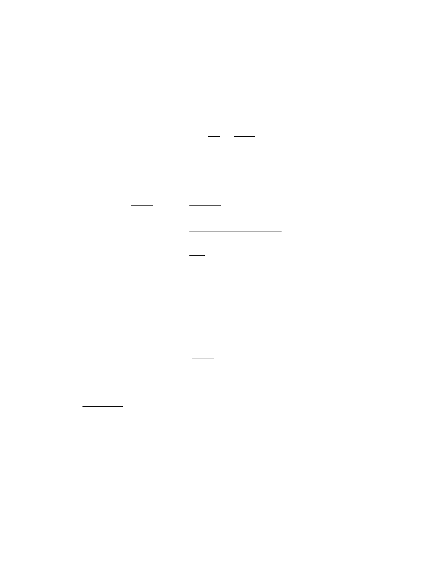
We can calculate winding numbers mathematically.
Lemma 12.4 (Winding Number Lemma)
Let γ be a closed contour, w ∈ C\γ. Then
n(γ, w) =
1
2πi
Z
γ
dz
z − w
.
Proof. If we write γ(t) = w + r(t)e
iθ(t)
, then r(t) and θ(t) are
continuous, piecewise continuous differentiable functions on
[a, b]
. We have,
Z
γ
dz
z − w
=
Z
b
a
γ
0
(t)
γ(t) − w
dt
=
Z
b
a
r
0
(t)e
iθ(t)
+ iθ
0
(t)r(t)e
iθ(t)
r(t)e
iθ(t)
dt
=
Z
b
a
r
0
(t)
r(t)
dt + i
Z
b
a
θ
0
(t) dt
= [log r(t)]
b
a
+ i [θ(t)]
b
a
= log r(a) − log r(b) + i (θ(a) − θ(b)) .
Now, γ is a closed contour and so γ(a) = γ(b), i.e. r(a)e
iθ(a)
=
r(b)e
iθ(b)
. Equating the moduli and arguments we get r(a) = r(b)
and θ(b) = θ(a) + 2πk for some k ∈ Z.
Putting these results into the integral above,
Z
γ
dz
z − w
= 2πik.
Moreover, θ(b)−θ(a) is the net increase in arg(γ(t)−w) as t runs
from a to b, so the number of times that γ winds round w is
θ(b) − θ(a)
2π
, i.e. k = n(γ, w).
Exercises 12.5
(i) Let γ be a closed contour and w ∈ C. Prove that n(−γ, w) =
−n(γ, w).
(ii) Let γ
1
and γ
2
be closed contours, so that the join can be
taken. Prove that n(γ
1
+ γ
2
, w) = n(γ
1
, w) + n(γ
2
, w)
An easy method of calculation
Calculating winding numbers can appear to be complicated to
calculate, you have to trace your finger round the curve bear-
ing in mind how many revolutions have been made. And you
have to do it for each region. Fortunately, there is an easier
56

method. In the examples above note that when passing from
one region to another via an edge (rather than via a crossing
of two line) the winding number for points in the regions only
changes by 1.
Now, consider the complicated contour image drawn below
with a line passing through it.
Start at the left side of the line. Obviously the winding num-
ber there is 0. As we go from left to right on the line we will
cross the contour. We apply the following rules:
• If we cross the contour so that it is travelling up, then the
winding number decreases by 1.
• If we cross the contour so that it is travelling down, then
the winding number increases by 1.
In the above diagram, the contour is travelling up when we
first meet it, so the point in the region we pass into have
winding number −1. At the next crossing the contour is going
down, and so the winding number of points in the next region
is 0. We can carry this out for all regions on the line. To get
other regions we can use different lines.
Exercise 12.6
Find the winding numbers for the points in the diagram.
Justification of the method
We can justify the method by considering two points w and z
that lie on opposite sides of a contour line that goes up. We
can assume that the contour starts and finishes at a point
near w and z. (If it didn’t we can do some reparametrisation
and join work.)
Now, take a loop C round w. Then, n(γ + C, w) = n(γ, z), as
the diagram shows. Thus,
n(γ + C, w) = n(γ, z)
n(γ, w) + n(C, w) =
n(γ, w) + 1 =
n(γ, w) = n(γ, z) − 1.
This shows that if we pass from z to w, then the winding num-
ber decreases by 1. Similarly, one can show an increase by 1
for a contour locally heading down.
57
Warning! 12.7
We have been using the image of the contour to calculate the
winding number of a point. Recall that the contour and its
image are different. Effectively, we have assumed that the
contour is traversed only once. If we go round the contour
twice, then the numbers calculated by eye have to be doubled.
More generally, if we go round k times, then we multiply the
‘by eye’ calculations by k.
Interior points
The method of counting the number of times a contour wraps
round a point helps define the notion of an interior point.
Definition 12.8
Let γ be a closed contour. The interior of γ is the set of points
w ∈ C\γ for which n(γ, w) 6= 0.
We denote the set of interior points of γ by Int(γ).
Example 12.9
The interior points of the contour in the next diagram are
shaded.
Example 12.10
Let γ(t) = w + Re
2πit
, 0 ≤ t ≤ 1. Then, Int(γ) = {z : |z − w| < R}.
Summary
• The winding number is the number of times a contour
wraps round a point in an anticlockwise direction.
• Let γ be a closed contour, w ∈ C\γ. Then
n(γ, w) =
1
2πi
Z
γ
dz
z − w
.
• It is easy to calculate a winding number by eye.
• An interior point is any point with non-zero winding num-
ber.
58
13
Cauchy’s (Fantastic) Theorem
We now come to the fundamental theorem in complex analy-
sis. There is no analogue in real analysis. It has far reaching,
deep consequences, and most of what we will prove from now
on relies on this theorem.
Theorem 13.1 (Cauchy’s Theorem)
Let D ⊆ C be a domain, and f : D → C be a differentiable
complex function. Let γ be a closed contour such that γ and
its interior points lie in D.
Then,
Z
γ
f = 0
.
Remarks 13.2
(i) This is truly a great theorem. It refers to any domain in
C, any analytic function on D, and any contour with all
interior points in D. And it says that any integral aris-
ing from this is zero. Thus, weak assumptions lead to a
strong conclusion.
(ii) It is important to note that the interior of γ lies within D.
If w is in the interior of γ but not in D, consider f (z) =
1/(z − w)
which is analytic on D = C\{w}, but
Z
γ
f =
Z
γ
dz
z − w
= 2πi n(γ, w) 6= 0,
so Cauchy’s theorem does not apply.
(iii) The proof of theorem is too complicated for the moment
and we will do it later. Note that we can’t just use the FTC
since we don’t know that f has an anti-derivative on D.
(iv) At first sight it may appear that the theorem will only
tell us about the behaviour of differentiable functions.
However, it has strong implications for non-differentiable
functions as well.
Exercise 13.3
Using the contours in Exercises 2 Question 1, to which of the
following integrals does Cauchy’s theorem apply? (There is no
need to evaluate them.)
Z
γ
1
|z|
2
dz,
Z
γ
1
z
2
z − 2
dz,
Z
γ
2
z dz,
Z
γ
2
+γ
3
sin
1
z − 1
dz.
59

The calculation trick
Recall, the trick I performed where I calculated an integral
over a path, before the path had even been defined. How was
this done?
The trick follows from Cauchy’s theorem and the funda-
mental example, (recall that the example says that
Z
γ
1
z
dz =
2πi
where γ is a small circle round the origin).
I was trying to integrate
Z
γ
a
z
dz
, where a was a number cho-
sen at random, and γ was a path chosen at random. However,
you were forced into choosing γ so that its winding number
was 1.
Now, we can take a small circle C going clockwise round
the origin, and we can make it so small that we can assume
it lies totally within the interior of γ. Now take another path
from the end of γ to the start of the circle C. Call this contour
β
.
Consider the contour Γ = γ + β + C − β. This is a closed
contour. Its interior does not include the disc encircled by C.
So it doesn’t contain the origin. But a/z is differentiable on
D = C\{0}, and the interior of Γ is a subset of D. Thus, we can
apply Cauchy’s theorem:
Z
Γ
a
z
dz = 0
Z
γ+β+C−β
a
z
dz = 0
Z
γ
a
z
dz +
Z
β
a
z
dz
Z
C
a
z
dz +
Z
−β
a
z
dz = 0
Z
γ
a
z
dz +
Z
β
a
z
dz
Z
C
a
z
dz −
Z
β
a
z
dz = 0
Z
γ
a
z
dz +
Z
C
a
z
dz = 0
Z
γ
a
z
dz = −
Z
C
a
z
dz
= a
Z
−C
1
z
dz
= a × 2πi
Z
γ
a
z
dz = 2aπi
60

Thus we get the answer expected. This method – of cutting
out a disc where the function is not defined – will be used
again later in more generality so make sure you understand
this simpler example.
Summary
• Let D ⊆ C be a domain, and f : D → C be a differentiable
complex function. Let γ be a closed contour such that γ
and its interior points lie in D.
Then,
Z
γ
f = 0
.
61
14
Strange Consequences of Cauchy’s Theorem
We will prove a number of surprising theorems that can be
deduced from Cauchy’s theorem.
(i) Cauchy’s Integral Formula: The value of a function at z
0
is determined by the values on a contour round z
0
.
(ii) Liouville’s Theorem: Any differential function bounded on
the whole of C is contant.
(iii) The Maximum Modulus Principle: The modulus of a func-
tion on a domain achieves its maximum on the boundary
of the domain.
(iv) Fudamental Theorem of Algebra: Every complex polyno-
mial has a complex root.
Cauchy’s Integral Formula
Theorem 14.1
Let D ⊆ C be a domain, and f : D → C be differentiable. Let
γ
be a closed contour such that γ and its interior points lie in
D
.
If w ∈ D\γ, then
Z
γ
f (z)
z − w
dz = 2πi n(γ, w)f (w).
Remarks 14.2
(i) If w is in the interior of γ, then
f (w) =
1
2πi n(γ, w)
Z
γ
f (z)
z − w
dz.
This says that the values of f inside γ are completely de-
termined by those on γ! Remarkable! This contrasts with
real analysis.
(ii) This behaviour is sometimes called ‘action at a distance’.
(iii) The special case f (z) = 1 for all z ∈ D gives the winding
number lemma.
Proof (of Theorem 14.1). Let γ
r
be the circular contour γ
r
=
w + re
it
, (0 ≤ t ≤ 2π), where r > 0 is sufficiently small so that γ
r
is contained in the interior of γ.
[Step 1] Let β be a contour in D\{w} from the start point of
γ
to the start point of γ
r
.
62

The contour
e
γ = γ + β + (−γ
r
) + · · · + (−γ
r
)
|
{z
}
n(γ,w)
times
+(−β),
where there are n(γ, w) copies of (−γ
r
)
, has winding number
zero about w, so by Cauchy’s theorem applied to
f (z)
z − w
on
D\{w}
,
Z
e
γ
f (z)
z − w
dz = 0
Z
γ
+
Z
β
−
Z
γ
r
− · · · −
Z
γ
r
+
Z
−β
f (z)
z − w
dz = 0
Z
γ
f (z)
z − w
dz − n(γ, w)
Z
γ
r
f (z)
z − w
dz = 0
Z
γ
f (z)
z − w
dz = n(γ, w)
Z
γ
r
f (z)
z − w
dz.
[Step 2] We shall now show that
lim
r→0
Z
γ
r
f (z)
z − w
dz = 2πif (w).
We have,
Z
γ
r
f (z)
z − w
dz = f (w)
Z
γ
r
dz
z − w
+
Z
γ
r
f (z) − f (w)
z − w
dz
= 2πif (w) +
Z
γ
r
f (z) − f (w)
z − w
dz,
by winding lemma.
Therefore
Z
γ
r
f (z)
z − w
dz − 2πif (w)
=
Z
γ
r
f (z) − f (w)
z − w
dz
≤ sup
z∈γ
r
f (z) − f (w)
z − w
× 2πr,
by the Estimation Lemma. Now
f (z) − f (w)
z − w
→ f
0
(w)
as z → w.
(Why does f
0
(w)
exist?) Hence RHS → |f
0
(w)|.0 = 0
as r → 0.
Therefore,
lim
r→0
Z
γ
r
f (z)
z − w
dz = 2πif (w).
Thus we can combine these steps to get
Z
γ
f (z)
z − w
dz − 2πin(γ, w)f (w) =
n(γ, w)
Z
γ
r
f (z)
z − w
dz
− 2πin(γ, w)f (w)
= n(γ, w)
Z
γ
r
f (z)
z − w
dz − 2πif (w)
.
63

The RHS tends to 0 as r → 0, but the LHS is independent of r
and so must be 0.
Examples 14.3
(i) Calculate
Z
γ
sin z
z − π
dz
, where γ(t) = 3e
−it
, 0 ≤ t ≤ 4π.
We apply CIF with f (z) = sin z and w = π. The point w lies
within the circle formed by γ, and n(γ, w) = −2, because γ
winds round w clockwise twice. (Draw a picture!)
Hence,
Z
γ
sin z
z − π
dz = 2πi × (−2) × sin(π) = −4πi.
(ii) Let γ be a circle of radius 2 about 2, i.e. z such that
|z − 2| = 2.
Draw the contour and indicate where the integrand is not
differentiable.
Then,
Z
|z−2|=2
e
z
z
2
− 9
dz =
Z
|z−2|=2
1
6
e
z
z − 3
−
1
6
e
z
z + 3
dz
=
1
6
Z
|z−2|=2
e
z
z − 3
dz −
1
6
Z
|z−2|=2
e
z
z + 3
dz
=
1
6
2πie
3
− 0, by 14.1,
=
iπe
3
3
.
Liouville’s Theorem
The next theorem is also rather surprising.
Theorem 14.4
Suppose f is differentiable on the whole of C, and is bounded,
i.e. there exists M such that |f (z)| ≤ M for all z ∈ C. Then, f
is constant.
64

Proof. [HTTLAM: We want to show the function is constant.
This is true if f (α) = f (0) for an arbitrary α. So we need to
show |f (α) − f (0)| = 0 for every α ∈ C.]
Let α ∈ C. We let R ≥ 2|α| and γ(t) = e
2πit
for 0 ≤ t ≤ 1 be a
circle of radius R round the origin. Then,
|f (α) − f (0)| =
1
2πi
Z
γ
f (z)
z − α
dz −
1
2πi
Z
γ
f (z)
z
dz
,
by CIF
=
1
2πi
Z
γ
f (z)
1
z − α
−
1
z
dz
=
1
2π
Z
γ
f (z)α
z(z − α)
dz
≤
1
2π
M sup
z∈γ
α
z(z − α)
L(γ)
by
≤
1
2π
M
|α|
R(R − |α|)
.2πR
=
M |α|
R − |α|
.
But R was effectively arbitrary, so as R → ∞, the LHS→ 0. As
neither f (α) nor f (0) depend on R we must have f (α)−f (0) = 0.
That is, f is constant.
Remark 14.5
Contrast this with real analysis. Being bounded does not im-
ply constant, for example, consider sin. This is differentiable
on all R and | sin x| ≤ 1 for all x ∈ R but it sin is not constant.
Exercise 14.6
Show cos and sin are not bounded on C.
Maximum Modulus Principle
Theorem 14.7
Let f : D → C be a differentiable function and γ be a closed
contour such that Int(γ) ⊂ D.
If |f (z)| ≤ M for all z ∈ γ, then |f (w)| ≤ M for all w ∈ Int(γ).
Remark 14.8
The theorem says that the modulus of a function within the
interior of a contour is never bigger than the modulus of the
function on the contour. In other words the maximum modu-
lus occurs on the boundary of a region.
65
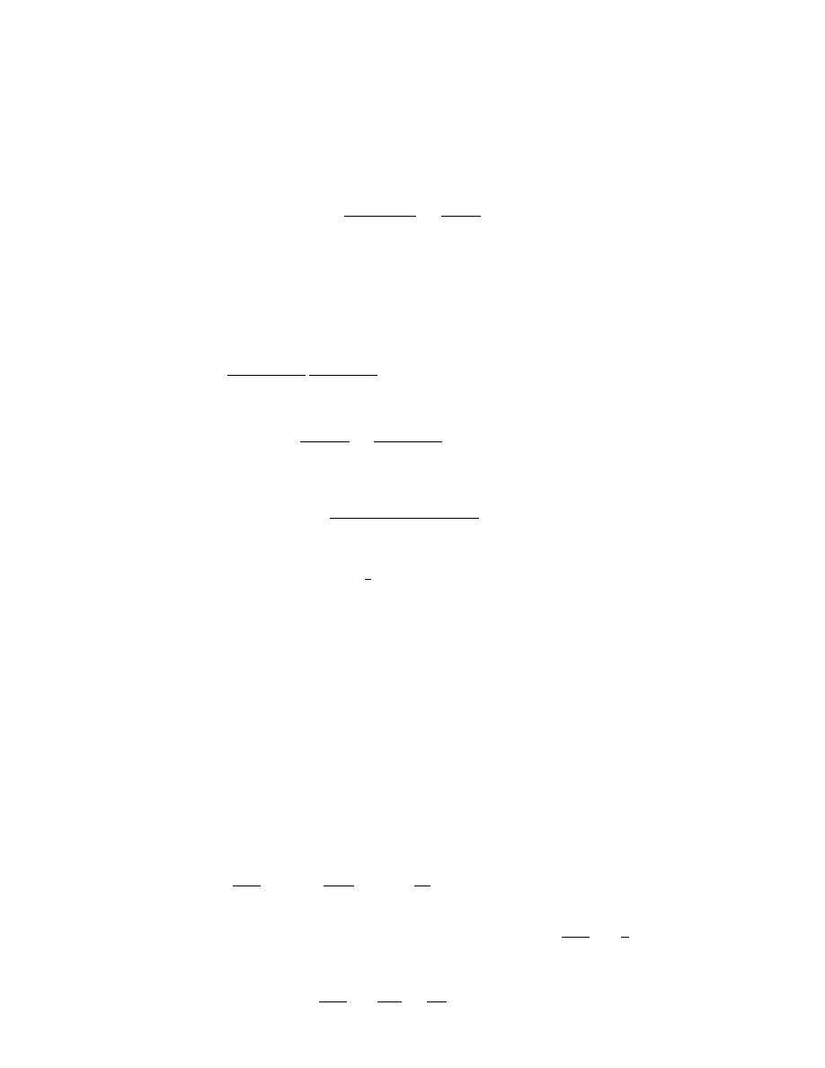
Proof. This proof contains a nice trick. We shall apply CIF to
w ∈ Int(γ)
and f (z)
k
, where k is a natural number:
f (w)
k
=
1
2πin(γ, w)
Z
γ
f (z)
k
z − w
dz.
Define the distance from w to γ by
dist(γ, w) = inf{|z − w| : z ∈ γ}.
Then, obviously |z − w| ≥ dist(γ, w) for all z ∈ γ.
So,
|f (w)|
k
≤
1
2π |n(γ, w)|
M
k
dist(γ, w)
L(γ),
by the Estimation Lemma,
since
|f (w)|
k
|z − w|
≤
M
k
dist(γ, w)
on γ.
Therefore,
|f (w)| ≤
L(γ)
2π |n(γ, w)| dist(γ, w)
1/k
M.
Now, we use the fact that lim
k→∞
x
1/k
= 1
for all x > 0, (this
is true because x
1/k
= exp(
1
k
ln x) → exp(0) = 1
). Thus, letting
k → ∞
gives |f (w)| ≤ M .
Fundamental Theorem of Algebra
We are now in a position to prove the Fundamental Theorem
of Algebra, (which is in fact not really a theorem of algebra but
of analysis!)
Theorem 14.9
Every polynomial p(z) = z
n
+ a
n−1
z
n−1
+ . . . a
1
z + a
0
, n ≥ 1, has a
root in C.
Proof. Suppose not and derive a contradiction. Since p(z) 6= 0
for all z ∈ C the function f defined by f(z) = 1/p(z) is differen-
tiable on all of C. Now, for z 6= 0,
p(z)
z
n
=
1 +
a
n−1
z
+ · · · +
a
0
z
n
→ 1 as |z| → ∞.
So there exists an R such that |z| ≥ R implies that
p(z)
z
n
≥
1
2
.
This in turn means
|f (z)| =
1
p(z)
≤
2
|z
n
|
≤
2
R
n
for |z| > R.
66

By the Maximum Modulus Principle applied to f with γ being
the standard circle of radius R round the origin we have |z| <
R =⇒ |f (z)| ≤
2
R
n
.
So |f (z)| ≤
2
R
n
on all of C. By Liouville’s theorem, f is con-
stant, and hence so is p. This is a contradiction, so p has a
root.
Summary
• Cauchy’s theorem can be used to prove surprising theo-
rems that have no analogues in real analysis.
• Cauchy’s Integral Formula: The value of a function at z
0
is determined by the values on contours round z
0
.
• Liouville’s Theorem: Any differential function bounded on
the whole of C is contant.
• The Maximum Modulus Principle: The modulus of a func-
tion on a domain achieves its maximum on the boundary
of the domain.
• Fudamental Theorem of Algebra: Every complex polyno-
mial has a complex root.
67

15
Taylor’s Theorem
Taylor’s theorem is a consequence of Cauchy’s theorem but is
so important we give it a separate section.
Theorem 15.1 (Taylor’s theorem for complex functions)
Suppose f : D → C is a differentiable function. Let z
0
∈ D and
R = dist(z
0
, C\D) (which equals infinity if D = C.) Then, there
exists a Taylor expansion of f about z
0
, i.e. there exist a
n
∈ C
such that
f (z) =
∞
X
0
a
n
(z − z
0
)
n
,
for all |z − z
0
| < R.
Furthermore,
a
n
=
f
(n)
(z
0
)
n!
=
1
2πi
Z
C
r
f (z)
(z − z
0
)
n+1
dz,
where C
r
is a small circle about z
0
and r is any number with
0 < r < R
.
Proof. Fix r with 0 < r < R. (We will replace z with z
0
+ h
so
that we have a power series in h centred at 0). For each h with
|h| < r, Cauchy’s Integral Formula gives
f (z
0
+ h) =
1
2πi
Z
C
r
f (z)
z − (z
0
+ h)
dz.
Now, with |h| < r and |z − z
0
| = r,
f (z)
z − (z
0
+ h)
=
f (z)
(z − z
0
)
1 −
h
z−z
0
=
f (z)
z − z
0
∞
X
n=0
h
z − z
0
n
=
∞
X
n=0
f (z)h
n
(z − z
0
)
n+1
.
Now we shall integrate term-by-term, (see Corollary 6.7), us-
ing g(z) =
f (z)
z − z
0
, and g
k
(z) =
f (z)h
n
(z − z
0
)
n+1
. Then, define M
k
by
M
k
=
sup
|z−z
0
|=r
|g
k
(z)| =
sup
|z−z
0
|=r
f (z)h
n
(z − z
0
)
n+1
=
sup
|z−z
0
|=r
|f (z)|
|h|
n
r
n+1
,
so,
P
∞
k=0
M
k
< ∞
as |h| < r. (Use the ratio test). Thus, by
68

Corollary 6.7,
Z
C
r
f (z)
z − (z
0
+ h)
dz =
∞
X
k=0
Z
C
r
f (z)h
n
(z − z
0
)
n+1
dz
2πif (z
0
+ h) =
∞
X
k=0
Z
C
r
f (z)
(z − z
0
)
n+1
dz
h
n
f (z
0
+ h) =
∞
X
k=0
1
2πi
Z
C
r
f (z)
(z − z
0
)
n+1
dz
h
n
Therefore, if we substitute z = z
0
+h
and let a
n
=
1
2πi
Z
C
r
f (z)
(z − z
0
)
n+1
dz
,
we get the series
f (z) =
∞
X
n=0
a
n
(z − z
0
)
n
.
That we also have a
n
=
f
(n)
(z
0
)
n!
follows from Corollary 10.6.
The theorem says that there exists an R-neighbourhood of z
0
upon which f is a power series. That is, f is analytic. This
explains why some authors use the word analytic to mean
complex differentiable:
differentiable and analytic are equivalent in complex analysis
.
Analytic and differentiable are not equivalent in real analy-
sis as we see in a later example.
The expression for a
n
is sometimes known as Cauchy’s for-
mula for derivatives.
HTTLAM 15.2
When solving problems concerning differentiable complex func-
tions, whether theoretical or practical ones, use the fact that
the function can be written locally as a power series.
Example 15.3
(i) Find the Taylor series of f (z) = (z + i)
3
at z = 0. We have,
f (z) = (z + i)
3
=⇒
f (0) = (0 + i)
3
= −i,
f
0
(z) = 3(z + i)
2
=⇒
f
0
(0) = 3(0 + i)
2
= −3,
f
00
(z) = 6(z + i)
=⇒
f
00
(0) = 6(0 + i) = 6i,
f
(3)
(z) = 6
=⇒
f
(3)
(0) = 6,
f
(4)
(z) = 0
=⇒
f
(4)
(0) = 0.
So,
f (z) = f (0) + f
0
(0)(z − 0) +
f
00
(0)
2!
(z − 0)
2
+
f
(3)
(0)
3!
(z − 0)
3
= −i − 3z + 3iz
2
+ z
3
.
69

Note that this expansion is valid for all z ∈ C as f is dif-
ferentiable on all of C, i.e. R = dist(0, C\C) = ∞.
(ii) Expand f (z) =
1
1 − z
about 0.
It is easy to show that
f
(n)
(z) =
n!
(1−z)
n+1
, so f
(n)
(0) = n!
.
Thus,
1
1 − z
= f (z) =
∞
X
n=0
f
(n)
(0)
n!
(z − 0)
n
=
∞
X
n=0
n!
n!
z
n
=
∞
X
n=0
z
n
.
This is valid for all |z| < 1 as f is differentiable on C\{1}
so R = dist(0, C\ (C\{1})) = dist(0, {1}) = 1.
Note that this confirms a result we already know.
Now we come to a very surprising and useful theorem, which
contrasts sharply with real differentiability.
Corollary 15.4 (Infinite Differentiability)
Suppose f : D → C is differentiable on the domain D. Then, f
is infinitely differentiable, i.e. it has derivatives of all orders.
Proof. Suppose z
0
is any point in D. From the theorem we
know that, in some neighbourhood of z
0
, f can be given as
a power series, and so is infinitely differentiable by Corollary
10.5.
This is really astounding. It doesn’t happen for real func-
tions as the next example illustrates.
Example 15.5
Suppose f : R → R is defined by
f (x) =
x
2
x > 0
0
x ≤ 0.
Then, f is differentiable with derivative
f (x) =
2x x > 0
0
x ≤ 0.
This derivative is not differentiable at 0, so f is not infinitely
differentiable.
Some facts about power series
We now use Taylor’s Theorem to prove some facts about series
which might otherwise be difficult to demonstrate.
70

Theorem 15.6
Suppose f (z) =
P
∞
n=0
a
n
z
n
for all |z| < R
1
and g(z) =
P
∞
n=0
b
n
z
n
for all |z| < R
2
. Then, f (z)g(z) = (f g)(z) =
P
∞
n=0
c
n
z
n
for all
|z| < min{R
1
, R
2
}, where c
n
=
P
n
k=0
a
k
b
n−k
.
Proof. Let R = min{R
1
, R
2
}. Then, f and g are complex dif-
ferentiable for all |z| < R. The product of two differentiable
functions is differentiable by the product rule. So, f g is dif-
ferentiable. By Theorem 15.1 it has a series expansion for
|z| < R, and by Corollary 10.6, we get
(f g)(z) =
∞
X
n=0
(f g)
(n)
(0)
n!
z
n
.
Now we can apply Leibnitz’s rule
(f g)
(n)
(0) =
n
X
k=0
n!
k!(n − k)!
f
(k)
(0)g
(n−k)
(0)
=
n
X
k=0
n!
f
(k)
(0)
k!
g
(n−k)
(0)
(n − k)!
= n!
n
X
k=0
a
k
b
n−k
.
Therefore,
(f g)(z) =
∞
X
n=0
c
n
z
n
, (|z| < R),
where c
n
=
n
X
k=0
a
k
b
n−k
.
Corollary 15.7
Suppose f and g are power series with positive radii of con-
vergence. If g(0) 6= 0, then f /g has a power series expansion at
0 with positive radius of convergence.
Proof. Define h(z) = 1/g(z). By continuity of g and the fact
that g(0) 6= 0, there is a ε-neighbourhood of 0 upon which h is
differentiable. Thus, h has a power series expansion, and the
result follows from the theorem applied to f h.
Remark 15.8
The precise value of the radius of convergence will depend on
where g is zero.
* Morera’s Theorem
There is a partial converse to Cauchy’s theorem. It relies on
the earlier optional material on the Fundamental Theorem of
Calculus.
71

Theorem 15.9
Let f : D → C be a continuous map on a connected domain D
such that
R
γ
f = 0
for all contours f . Then, f is differentiable.
Proof. We know from Theorem 9.9 that there exists F : D → C
such that F
0
= f
. But by Corollary 15.4 the derivative of a
differentiable function is itself differentiable.
Summary
• If a complex function is differentiable on a domain, then
at every point there is power series expansion valid on
some ε-neighbourhood.
• Differentiable complex functions are infinitely differentiable.
• If S
1
and S
2
are power series with radii of convergence R
1
and R
2
, then S
1
S
2
is a power series with radius of conver-
gence min{S
1
, S
2
}.
• If S is a power series at z
0
with positive radius of conver-
gence, then 1/S has a power series expansion at z
0
pro-
vided S(z
0
) 6= 0
.
• There is a partial converse to Cauchy’s Theorem.
72

16
Zeros of functions
We have met a number of functions that are not analytic (i.e.
differentiable) at certain points. For example, 1/z is not ana-
lytic at 0, because it is undefined when z is zero. Therefore, it
seems natural to investigate zeros of functions first.
Zeros
Definition 16.1
An analytic function f : D → C has a zero at z
0
if f (z
0
) = 0
.
Examples 16.2
(i) The function sin has zeros at kπ, for all k ∈ Z.
(ii) By Theorem 1.35(iv) f (z) = e
z
has no zeros.
(iii) f (z) = z
3
(z
2
+ 1)
has a zero at z = i, one at z = −i, and one
at z = 0.
Exercise 16.3
Find the zeros of:
(i) z
2
+ 9,
(ii) e
z
2
+9
(z + 4i),
(iii) e
z−2
− 1.
We now know that if f : D → C is differentiable at z
0
, it has
a Taylor series expansion about z
0
: f (z) =
P
∞
n=0
a
n
(z − z
0
)
n
for
all z with |z − z
0
| < R for some R > 0.
Definition 16.4
We say f has a zero of order m at z
0
if
a
0
= a
1
= · · · = a
m−1
= 0
but a
m
6= 0.
Remark 16.5
Obviously, by Theorem 15.1, f has a zero of order m at z
0
if
and only if f
(j)
(z
0
) = 0
for all j < m and f
(m)
(z
0
) 6= 0
.
In particular, if f (z
0
) = 0
and f
0
(z
0
) 6= 0
, then f has a zero of
order 1.
Examples 16.6
(i) The function f (z) = z
2
has a zero of order 2 at 0.
(ii) The function f (z) = z(z + 2i)
3
has a zero of order 1 at 0 and
one of order 3 at −2i.
(iii) More generally, suppose that f is a polynomial with a root
of multiplicity m at z
0
. Then, f has a zero of order m at z
0
.
73

Exercise 16.7
Find the zeroes and their orders of the following:
(i) (z −1)
3
(z +1)
(ii) (z
2
+1)
2
,
(iii) ze
z
2
,
(iv) (2z −3i)
4
,
(v) z
3
+1.
Exercise 16.8
Suppose that f : D → C is an analytic function with a zero
of order m at z
0
. Then, there exists a differentiable g and an
R > 0
, such that f (z) = (z − z
0
)
m
g(z)
, for all |z − z
0
| < R, and
g(z
0
) 6= 0
.
Summary
• An analytic function f : D → C has a zero at z
0
if f (z
0
) = 0
.
• Suppose f (z) =
P
∞
n=0
a
n
(z − z
0
)
n
for all z with |z − z
0
| < R
for some R. Then f has a zero of order m at z
0
if
a
0
= a
1
= · · · = a
m−1
= 0
but a
m
6= 0.
74
17
Poles
The notions of pole and residue are crucial to the application
of complex analysis to real problems, such as real integrals,
or Fourier and Laplace Transforms
7
. We define poles in this
section and show how to locate them in the next. After that
we define their residue.
A motivating example
Let us consider an example: Integrate
Z
|z|=1
e
z
z
2
dz
, where |z| = 1
denotes the standard contour of a unit circle round the origin.
We can’t use Cauchy’s Integral Formula as the integrand is
not analytic at 0 and the Fundamental Theorem of Calculus
doesn’t help as we can’t see any obvious antiderivative.
Let’s just integrate term-by-term
8
and see what happens.
Z
|z|=1
e
z
z
2
dz =
Z
|z|=1
1
z
2
1 + z +
z
2
2!
+
z
3
3!
+ . . .
dz
=
Z
|z|=1
1
z
2
+
1
z
+
1
2
+
z
6
+ . . .
dz
=
Z
|z|=1
1
z
2
dz +
Z
|z|=1
1
z
dz +
Z
|z|=1
1
2
dz +
Z
|z|=1
z
6
dz + . . .
= 0 + 2πi + 0 + 0 + . . . .
Notice that only the 1/z term mattered. By the Fundamen-
tal Example, all the other terms were irrelevant. This is key
to understanding the terms pole and residue we are going to
define.
Laurent expansions
First we shall look at functions, like the integrand e
z
/z
2
exam-
ple above, that can be represented by a series with negative
powers.
Recall for an analytic function we can represent it as
f (z) =
∞
X
n=0
a
n
(z − z
0
)
n
for |z − z
0
| < R.
Compare this with the following series.
7
These transforms are used in Applied Mathematics. If you know what they are, then fine.
If not, then don’t worry about it.
8
Obviously, we should check that we can do this!
75

Definition 17.1
Suppose that f : D → C is complex function. Then we say f
has a Laurent expansion at z
0
if there exist a
n
∈ C and R > 0,
such that
f (z) =
∞
X
n=−∞
a
n
(z − z
0
)
n
for all z with 0 < |z − z
0
| < R.
Note that the limits go from −∞ to ∞, and that the expansion,
does not necessarily equal f (z
0
)
when z = z
0
, (which may be
undefinable anyway).
Example 17.2
(i) f (z) = 1/z has an expansion at 0 with a
n
= 0
for n 6= −1,
a
−1
= 1
, and R = ∞.
(ii) The expansion of f (z) = e
z
/z
2
at 0,
e
z
z
2
=
1
z
2
+
1
z
+
1
2
+
z
6
+ . . .
has a
n
=
1
(n + 2)!
for n ≥ 0, a
−1
= a
−2
= 1
, and a
j
= 0
for
j ≤ −3
. The radius is R = ∞.
(iii) Any power series with a positive radius of convergence is
a Laurent expansion. Hence, any function differentiable
at z
0
has a Laurent expansion.
Exercise 17.3
Find a Laurent expansion for f (z) =
sin z
z
4
defined on C\{0}.
The definition of a pole
Definition 17.4
Suppose that f : D → C is a complex function. We say that
f
has a pole of order N at z
0
∈ D, if there exists a Laurent
expansion at z
0
of the form
f (z) =
∞
X
n=−N
a
n
(z − z
0
)
n
(0 < |z − z
0
| < R), with a
−N
6= 0.
Poles are also called singularities.
If there is no N ≥ 0 such that a
n
= 0
for all n < −N , then we
say f has an essential singularity at z
0
.
Remark 17.5
The point is that for a pole of finite order there are only a finite
number of negative exponents of z in the series.
76

Examples 17.6
(i) order(1/z
5
) = 5
at 0.
(ii) order(e
z
/z
2
) = 2
at 0 as f (z) =
1
z
2
+
1
z
+
1
2
+
z
6
+ . . .
.
(iii) order
i
(z − 4i)
3
+ (z − 4i)
2
− 2i(z − 4i)
5
= 3
at 4i.
(iv) f (z) = exp(1/z) has an essential singularity at 0 because
f (z) =
∞
X
n=0
(1/z)
n
n!
=
∞
X
n=0
z
−n
n!
=
0
X
n=−∞
z
n
(−n)!
,
and this obviously has an infinite number of terms with
negative exponent.
Remarks 17.7
(i) If such a Laurent series exists, then the coefficients are
unique. To see this look at (z − z
0
)
N
f (z)
, this is a power
series and so has unique coefficients.
(ii) Suppose that f (z) has a Laurent expansion with N = 0,
i.e.
f (z) = a
0
+ a
1
(z − z
0
) + a
2
(z − z
0
)
2
+ . . .
for 0 < |z − z
0
| < R.
Then, we can define f (z
0
) = a
0
and thus make f analytic
at z
0
.
If we can do this, we say f has a removable singularity.
Example 17.8
The function f (z) =
sin z
z
is defined on C\{0}, and we have
f (z) =
sin z
z
=
1
z
z −
z
3
3!
+
z
5
5!
− . . .
= 1 −
z
2
3!
+
z
4
5!
− . . . .
So define f (0) = 1 to make f analytic on all of C. That is,
f (z) =
(
sin z
z
,
for z 6= 0,
1,
for z = 0.
Exercise 17.9
Show that (e
z
− 1)/z has a removable singularity.
77

Summary
• An expansion of f of the form
f (z) =
∞
X
n=−∞
a
n
(z − z
0
)
n
for all z with 0 < |z − z
0
| < R, is called a Laurent expansion
at z
0
.
• We say that f has a pole of order N at z
0
∈ D, if there
exists a Laurent expansion at z
0
of the form
f (z) =
∞
X
n=−N
a
n
(z − z
0
)
n
(0 < |z − z
0
| < R), with a
−N
6= 0.
78
18
How to find poles
It is hard to give non-trivial examples of poles without using
some theory. You may have noticed that the order is somehow
connected with the order of multiplicity of the polynomial in a
denominator. The following puts that intuition into a precise
mathematical statement, and does it for general functions not
just polynomials.
Lemma 18.1
Suppose that f (z) =
p(z)
q(z)
, where
(i) p is analytic at z
0
, and p(z
0
) 6= 0
,
(ii) q is analytic at z
0
, and has a zero of order N at z
0
.
Then, f has a pole of order N at z
0
.
Proof. By assumption, we have q(z) = (z − z
0
)
N
r(z)
where r(z)
is analytic with r(z
0
) 6= 0
(see Exercise 16.8). Then, g(z) =
p(z)
r(z)
is analytic at z
0
, so by Theorem 15.1 it has a power series
expansion:
g(z) =
∞
X
n=0
a
n
(z − z
0
)
n
,
valid for |z − z
0
| < R, some R > 0.
Thus,
f (z) =
p(z)
q(z)
=
p(z)
(z − z
0
)
N
r(z)
=
g(z)
(z − z
0
)
N
=
1
(z − z
0
)
N
∞
X
n=0
a
n
(z − z
0
)
n
=
a
0
(z − z
0
)
N
+
a
1
(z − z
0
)
N −1
+
a
2
(z − z
0
)
N −2
+ . . .
But,
a
0
= g(z
0
) =
p(z
0
)
r(z
0
)
6= 0,
because p(z
0
) 6= 0
by assumption and r(z
0
) 6= 0
by definition.
So as a
0
6= 0, we deduce that f has a pole of order N at z
0
.
79

Common Error 18.2
The above lemma gives a method for finding a pole and its
order. The definition of a pole is that given in Definition 17.4.
It is not the multiplicity of the denominator in an expression.
Do not confuse the definition of an object with a process by
which we find the object.
Remark 18.3
Recall that a zero of order N of a polynomial is just a root of
multiplicity N .
Example 18.4
(i) The function
sin z
(z − 3)
2
has a pole of order 2 at z = 3, since
sin
is analytic and sin 3 6= 0, and (z − 3)
2
is analytic with a
root of multiplicity 2 at 3.
(ii) The quotient
z(z − 1)
4
(z
2
− 2z + 5)
2
has poles of order 2 at z = 1±2i.
This is because we can factorize the polynomial z
2
− 2z + 5
to get (z − (1 + 2i))(z − (1 − 2i)). The resulting roots are
repeated as
(z
2
− 2z + 5)
2
= [(z − (1 + 2i))]
2
[(z − (1 − 2i))]
2
.
Exercises 18.5
Find the poles and their orders for
(a)
1 + e
z
z(z
2
− 1)
,
(b)
1 + z
z
3
− 2z
2
,
(c)
e
z
2
− 1
z
5
(It ain’t 5!)
Simple poles
Poles of order 1 are given a special name.
Definition 18.6
A pole of order 1 is called a simple pole.
Example 18.7
(i) 1/z has a simple pole at 0.
(ii)
sin z
z
2
has a simple pole at 0:
sin z
4z
2
=
z −
z
3
3!
+
z
5
5!
− . . .
4z
2
=
1
4z
−
z
3!4
+
z
3
5!4
− . . . .
80

There is a useful way of locating simple poles.
Theorem 18.8
Suppose f (z) =
p(z)
q(z)
where,
(i) p is analytic at z
0
, and p(z
0
) 6= 0
,
(ii) q is analytic at z
0
, q(z
0
) = 0
and q
0
(z
0
) 6= 0
.
Then, f has a simple pole at z
0
.
Proof. By Remark 16.5 q has a zero of order 1 at z
0
. Thus,
by Lemma 18.1, f has a pole of order 1 at z
0
, i.e. the pole is
simple.
Examples 18.9
(i) The function f (z) =
cos z
z
has a simple pole at 0. We have
p(z) = cos z
and q(z) = z, so p(0) = 1, q(0) = 0, and q
0
(0) = 1
.
(ii) The function f (z) =
z + 3
sin z
has a simple pole at 0. We have
p(z) = z + 3
and q(z) = sin z, so p(0) = 3, q(0) = 0, and
q
0
(0) = cos 0 = 1
.
Summary
• Suppose that f (z) =
p(z)
q(z)
, where
(i) p is analytic at z
0
, and p(z
0
) 6= 0
,
(ii) q is analytic at z
0
, and has a zero of order N at z
0
.
Then, f has a pole of order N at z
0
.
• A simple pole is a pole of order 1.
81

19
Residues
We saw earlier that to integrate
e
z
z
2
=
1
z
2
+
1
z
+
1
2
+
z
6
. . .
we could use the Laurent expansion about zero to integrate
term-by-term. The only information that mattered was the
coefficient of the z
−1
term. Let us now give that term an official
name.
Definition 19.1
Suppose that f has a pole at z
0
. The residue of f at z
0
is
the coefficient a
−1
in the expansion
P
∞
n=−N
a
n
(z − z
0
)
n
. This is
denoted res(f, z
0
)
.
Examples 19.2
(i) res(e
z
/z
2
, 0) = 1
.
(ii) res(z
2
, 0) = 0
. (The residue is always 0 at differentiable
points.)
(iii) From earlier,
sin z
4z
2
=
1
4z
−
z
3!4
+
z
3
5!4
− . . .
so res
sin z
4z
2
, 0
=
1
4
.
Remark 19.3
The residue at a point is unique because the coefficients of a
Laurent expansion with a finite number of negative terms are
unique.
The next theorem gives a hint of where we are going with
residues: They allow us to quickly calculate integrals. This
theorem is really just generalising the example of e
z
/z
2
used
at the start of the section on poles.
Theorem 19.4 (Cauchy’s Residue Theorem for a Circle)
Suppose that the analytic function f : D → C has a pole at p.
Let γ(p, r) denote the circle of radius r round p. Then, there
exists R > 0 such that
Z
γ(p,r)
f (z) dz = 2πi res(f, p),
for all 0 < r < R.
82

Proof. At p the function f has a Laurent expansion f (z) =
P
∞
n=−N
a
n
(z − p)
n
, for 0 < |z − p| < R, some R > 0. Therefore, let
r
be such that 0 < r < R, and then
Z
γ(p,r)
f (z) dz =
Z
γ(p,r)
∞
X
n=−N
a
n
(z − p)
n
dz
=
∞
X
n=−N
Z
γ(p,r)
a
n
(z − p)
n
dz.
The latter equality follows from Theorem 6.7 (you can check
this!). But, by the Fundamental Example,
Z
γ(p,r)
a
n
(z − p)
n
dz = a
n
Z
γ(p,r)
(z − p)
n
dz
=
a
−1
× 2πi, n = −1
0,
n 6= −1.
Thus,
R
γ(p,r)
f (z) dz = 2πia
−1
= 2πi res(f, p)
.
Remark 19.5
The theorem says that to calculate certain integrals all we
have to do is calculate the residue of a function at a point.
Example 19.6
Let γ be the unit circle round the origin. We take f (z) = e
z
/z
2
from earlier, then res(f, 0) = 1 has already been calculated. So
R
γ
e
z
/z
2
= 2πi res(f, 0) = 2πi
, as we have already seen.
We shall generalise the theorem further, but in the next
section we will see investigate some methods for calculating
residues.
Summary
• The residue of f at z
0
is the coefficient a
−1
in the expan-
sion
P
∞
n=−N
a
n
(z − z
0
)
n
. This is denoted res(f, z
0
)
.
• Suppose that the analytic function f : D → C has a pole at
p
. Let γ(p, r) denote the circle of radius r round p. Then,
there exists R > 0 such that
Z
γ(p,r)
f (z) dz = 2πi res(f, p),
for all 0 < r < R.
83

20
Bluffer’s Guide to Calculating Residues
Residues are an important part of any course on Complex
Analysis. They allow us to easily calculate otherwise com-
plicated integrals – without doing any integration!
This section contains the main methods for calculating the
residues of poles. You should know them and their proofs.
Method 1: Simple Poles
Suppose f has a simple pole (i.e. order 1) at w then
res(f, w) = lim
z→w
(z − w)f (z).
Proof. As f has a simple pole at w we have
f (z) =
∞
X
n=−1
a
n
(z − w)
n
.
So,
lim
z→w
(z − w)f (z)
=
lim
z→w
(z − w)
∞
X
n=−1
a
n
(z − w)
n
=
lim
z→w
(z − w)
a
−1
z − w
+ a
0
+ a
1
(z − w) + a
2
(z − w)
2
+ . . .
=
lim
z→w
a
−1
+ a
0
(z − w) + a
1
(z − w)
2
+ a
2
(z − w)
3
+ . . .
= a
−1
=
res(f, w).
Examples 20.1
(i) The function f (z) =
sin(z)
z − 3
has a pole of order 1 at z = 3, so
res(f, 3) = lim
z→3
(z−3)f (z) = lim
z→3
(z−3)
sin(z)
z − 3
= lim
z→3
sin(z) = sin(3).
(ii) The function f (z) =
z
1 − cos z
has a pole of order 1 at z = 0,
so
res(f, 0) = lim
z→0
z
z
1 − cos z
= lim
z→0
z
2
2 sin
2
(z/2)
= lim
z→0
4 (z/2)
2
2 sin
2
(z/2)
= 2 lim
z→0
z/2
sin(z/2)
2
= 2
lim
z→0
z/2
sin(z/2)
2
= 2.
84

Method 2: Some quotients (Really good method!)
Suppose f (z) =
p(z)
q(z)
with p and q analytic, p(w) 6= 0, q(w) = 0
and q
0
(w) 6= 0
. Then,
res(f, w) =
p(w)
q
0
(w)
.
Proof. By Theorem 18.8 f has a simple pole at w, so
res(f, w) =
lim
z→w
(z − w)f (z),
by Method 1,
=
lim
z→w
(z − w)
p(z)
q(z)
=
lim
z→w
p(z)
q(z)
z − w
=
lim
z→w
p(z)
q(z) − q(w)
z − w
,
as q(w) = 0,
=
lim
z→w
p(z)
lim
z→w
q(z) − q(w)
z − w
=
p(w)
q
0
(w)
,
by definition of differentiation.
Remark 20.2
The conditions imply that f has a simple pole, so the method
will only work in this case.
Examples 20.3
(i) The function f (z) =
1
1 − z
3
has a pole at z = 1. We have
p(z) = 1
and q(z) = 1 − z
3
so q
0
(1) = −3 × 1
2
= −3
. Thus
res(f, 1) =
p(1)
q
0
(1)
=
1
−3
= −
1
3
.
(ii) The function f (z) =
2z
2
1 + z
4
has a pole at z = e
iπ/4
(and
more besides, but we’ll ignore them). Let p(z) = 2z
2
and
q(z) = 1 + z
4
. Then p(e
iπ/4
) = 2e
iπ/2
6= 0; q
0
(z) = 4z
3
so
q
0
(e
iπ/4
) = 4e
3iπ/4
6= 0. So
res f, e
iπ/4
=
p(e
iπ/4
)
q
0
(e
iπ/4
)
=
2e
iπ/2
4e
3iπ/4
=
e
−iπ/4
2
=
1
4
(1 − i)
√
2.
85
Method 3: Poles of order N
We now generalise Method 1 (which is the case N = 1 in the
following).
Suppose that f has a pole of order N at w. Then
res(f, w) =
1
(N − 1)!
lim
z→w
d
N −1
dz
N −1
(z − w)
N
f (z)
.
Proof. By assumption f (z) =
P
∞
n=−N
a
n
(z − w)
n
for some a
i
∈ C
and 0 < |z − w| < R. Thus,
f (z) =
∞
X
n=−N
a
n
(z − w)
n
(z − w)
N
f (z) = (z − w)
N
a
−N
(z − w)
N
+ · · · +
a
−1
z − w
+ a
0
+ a
1
(z − w) + . . .
= a
−N
+ a
−N +1
(z − w) + · · · + a
−1
(z − w)
N −1
+a
0
(z − w)
N
+ . . . .
Therefore,
1
(N − 1)!
lim
z→w
d
N −1
dz
N −1
(z − w)
N
f (z)
=
1
(N − 1)!
lim
z→w
d
N −1
dz
N −1
a
−N
+ a
−N +1
(z − w) + . . .
+a
−1
(z − w)
N −1
+ a
0
(z − w)
N
+ . . .
=
1
(N − 1)!
lim
z→w
{(N − 1)! a
−1
+ N ! a
0
(z − w) + . . . }
=
1
(N − 1)!
(N − 1)! a
−1
= a
−1
=
res(f, w).
Examples 20.4
(i) Let f (z) =
z + i
z − i
2
. By Lemma 18.1 this has a pole of
order 2 at z = i. Hence,
res(f, i) =
1
(2 − 1)!
lim
z→i
d
2−1
dz
2−1
(
(z − i)
2
z + i
z − i
2
)
= 1. lim
z→i
d
dz
(z + i)
2
= lim
z→i
2(z + i)
= 2(i + i)
= 4i.
86

(ii) The function f (z) =
e
e
z
z
2
has a pole of order 2 at z = 0,
(again by Lemma 18.1). So,
res(f, 0) =
1
1!
lim
z→0
d
dz
z
2
e
e
z
z
2
= lim
z→0
d
dz
e
e
z
= lim
z→0
e
z
.e
e
z
= e.
Method 4: Direct expansion
We can use this as a last resort. We expand functions as power
series, etc., and then calculate coefficients.
Examples 20.5
(i) Let f (z) =
ze
z
(z − 1)
3
. This has a pole of order 3 at z = 1. So,
expand about w = 1: (i.e. let z = w + h and take h as our
variable),
f (1 + h) =
(1 + h)e
1+h
(1 + h − 1)
3
= (1 + h)
e.e
h
h
3
=
e
h
3
(1 + h)
1 + h +
h
2
2!
+
h
3
3!
+ . . .
=
e
h
3
1 + 2h +
3
2
h
2
+
2
3
h
3
+ . . .
=
e
h
3
+
2e
h
2
+
3e
2h
+
2e
3
+ . . .
So res(f, 1) =
3e
2
.
(ii) ∗ Find res
π cot πz
z
2
, 0
.
We expand about w = 0:
π cot π(0 + h)
(0 + h)
2
=
π cot πh
h
2
=
π
h
2
cos πh
sin πh
=
π
h
2
(1 − (πh)
2
/2! + . . . )
(πh − (πh)
3
/3! + . . . )
=
1
h
3
(1 − π
2
h
2
/2 + . . . )
(1 − π
2
h
2
/6 + . . . )
.
Consider the parts in brackets, this quotient will be a
power series and so we need to work out its coefficients.
87

We need only work out the coeffient for h
2
since division
by the h
3
will give the residue coefficient.
We work with the bottom bracket first.
Suppose that
(1 − π
2
h
2
/6 + . . . )
−1
= b
0
+ b
1
h + b
2
h
2
+ . . .
. Then,
1 − π
2
h
2
/6 + . . .
1 − π
2
h
2
/6 + . . .
−1
= 1
1 − π
2
h
2
/6 + . . .
b
0
+ b
1
h + b
2
h
2
+ . . .
= 1
b
0
+ b
1
h + b
2
h
2
−
π
2
h
2
6
b
0
+ b
1
h + b
2
h
2
+ . . . = 1
b
0
+ b
1
h +
b
2
−
π
2
6
b
0
h
2
+ . . . = 1.
Equating coefficients gives b
0
= 1
, b
1
= 0
and b
2
−
π
2
6
b
0
= 0
,
i.e. b
2
=
π
2
6
.
Therefore,
π cot πh
h
2
=
1
h
3
1 −
π
2
h
2
2
+ . . .
1 −
π
2
h
2
6
+ . . .
−1
=
1
h
3
1 −
π
2
h
2
2
+ . . .
1 +
π
2
h
2
6
+ . . .
=
1
h
3
1 −
π
2
3
h
2
+ . . .
=
1
h
3
−
π
2
3h
+ . . .
Thus res(f, 0) = −
π
2
3
.
Obviously, this method can get a bit calculation heavy.
Summary
• Simple pole: res(f, w) = lim
z→w
(z − w)f (z)
.
• Some quotients: Suppose p(w) 6= 0, q(z) = 0 and q
0
(w) 6= 0
.
Then,
res
p
q
, w
=
p(w)
q
0
(w)
.
• Pole of order N :
res(f, w) =
1
(N − 1)!
lim
z→w
d
N −1
dz
N −1
(z − w)
N
f (z)
.
• Calculate expansions directly, equate coefficients, etc.
88

21
Cauchy’s Residue Formula
The next theorem shows that we can calculate certain com-
plex integrals by merely calculating the residues and winding
numbers at poles. Thus we have a very simple five-finger-
exercise method for calculating integrals. Hooray!
Theorem 21.1 (Cauchy’s Residue Formula)
Let D be domain and γ a closed contour such that Int(γ) ⊆ D.
Let {p
1
, . . . , p
m
} ∈ D\γ and f : D → C be analytic with poles at
p
1
, . . . , p
m
. Then
Z
γ
f (z) dz = 2πi
m
X
j=1
n(γ, p
i
) res(f, p
j
).
Proof. We can assume that all the poles are in the interior of
γ
. Now, consider the following sketch.
Let C
j
be a circle of radius ε > 0 at p
j
, taken clockwise.
Then, there exists ε > 0 such that C
j
⊆ Int(γ) and C
j
∩ C
l
= ∅
for all j and l with j 6= l and so that C
j
lies within the disc
upon which the Laurent expansion for f at p
j
holds.
There exist contours β
j
from some point on the image of γ
to the start of C
j
. We can define γ
j
as the part of γ from the
start of β
j
to β
j+1
. So γ = γ
1
+ · · · + γ
m
.
Next, we define a contour
e
γ
by
e
γ = β
1
+ n(γ, p
1
)C
1
− β
1
+ γ
1
+β
2
+ n(γ, p
2
)C
2
− β
2
+ γ
2
+ . . .
+β
m
+ n(γ, p
m
)C
m
− β
m
+ γ
m
.
This is a path such that f is analytic on Int(
e
γ)
, (just like in
the calculation trick I did.) So by Cauchy’s Theorem we have
R
e
γ
f = 0
. But
Z
e
γ
f
= n(γ, p
1
)
Z
C
1
f + n(γ, p
2
)
Z
C
2
f + · · · + n(γ, p
m
)
Z
C
m
f +
Z
γ
1
+...γ
m
f
0 =
m
X
j=1
n(γ, p
j
)
Z
C
j
f
!
+
Z
γ
1
+...γ
m
f.
Note that the integrals over all the β
j
cancel. So, as γ = γ
1
+
89

· · · + γ
m
we get,
0 =
m
X
j=1
n(γ, p
j
)
Z
C
j
f
!
+
Z
γ
f
−
m
X
j=1
n(γ, p
j
)
Z
C
j
f
=
Z
γ
f
m
X
j=1
n(γ, p
j
)
Z
−C
j
f
=
Z
γ
f.
But, by Theorem 19.4,
R
−C
j
f = 2πi res(f, p
j
)
. Thus the proof is
complete.
There we have it, one of the best theorems in mathematics!
Examples 21.2
Evaluate the integral
Z
γ
1
z
2
+ (i − 1)z − i
dz
, where γ is a square
with sides of length 4 centred at the origin, oriented anti-
clockwise.
Solution: Let f (z) =
1
z
2
+ (i − 1)z − i
=
1
(z + i)(z − 1)
. There-
fore, f has simple poles at z = 1 and z = −i.
Let q(z) =
z
2
+(i−1)z−i
, then q
0
(z) = 2z+i−1
. We have q
0
(1) = 2+i−1 = 1+i
,
and q
0
(−i) = −2i + i − 1 = −1 − i
. Thus,
res(f, 1) =
1
1 + i
=
1 − i
2
and res(f, −i) =
1
−1 − i
=
−1 + i
2
.
We have n(γ, 1) = n(γ, −i) = 1, so by Cauchy’s Residue Theorem
Z
γ
1
z
2
+ (i − 1)z − i
dz = 2πi ( res(f, 1) + res(f, −i))
= 2πi
1 − i
2
+
−1 + i
2
= 0.
Summary
• Let D be domain and γ a closed contour such that Int(γ) ⊆
D
. Let {p
1
, . . . , p
m
} ∈ D\γ and f : D → C be analytic with
poles at p
1
, . . . , p
m
. Then
Z
γ
f (z) dz = 2πi
m
X
j=1
n(γ, p
i
) res(f, p
j
).
90

22
Evaluation of Definite Real Integrals
We shall now see that complex analysis allows us to solve, in
a simple manner, problems involving real functions that are
not easy to solve with real methods.
The basic idea
We want to calculate
R
∞
−∞
f (x) dx
where f is a real function. The
basic method is actually quite simple, but it has a number of
parts, so may initially appear complicated. First, I’ll outline
the ideas behind it.
Let us note that we can calculate the real integral as a con-
tour integral. Let Γ
1
(t) = t
, then Γ
0
(t) = 1
for −R ≤ t ≤ R.
So,
Z
Γ
1
f (z)dz =
Z
R
−R
f (t).1 dt =
Z
R
−R
f (t) dt.
If we let R → ∞, then we usually obtain the real integral
R
∞
−∞
f (x) dx
(but see Remark 22.3 later).
This doesn’t really get us much further forward. However,
if we take a contour Γ
R
from R to −R via a path in the complex
plane and join it to Γ
1
, then we get a closed contour. Thus, we
can use Cauchy’s Residue Theorem to calculate the integral.
Consider the following diagram in the complex plane, where
Γ
R
is the semi-circle in the upper half-plane.
If we integrate round the contour Γ = Γ
1
+ Γ
R
, then we get
Z
Γ
f (z) dz =
Z
Γ
1
f (z) dz +
Z
Γ
R
f (z) dz.
Now, letting R → ∞, we get
lim
R→∞
Z
Γ
f (z) dz =
lim
R→∞
Z
Γ
1
f (z) dz + lim
R→∞
Z
Γ
R
f (z) dz
=
lim
R→∞
Z
R
−R
f (t) dt + lim
R→∞
Z
Γ
R
f (z) dz
=
Z
∞
−∞
f (x) dx + lim
R→∞
Z
Γ
R
f (z) dz.
Now, the LHS is a contour integral for a closed contour and
so by Cauchy’s Residue Formula we can probably work it out
using some method. The RHS contains the integral we want.
Great! It also contains another term. Not so great! However,
if that term is zero, then we have a way of calculating a real
integral from residues!
91

Can we show that the integral
R
Γ
R
f (z) dz → 0
as R → ∞?
The following lemma gives us a supply of examples with this
property.
Lemma 22.1 (Jordan’s Lemma)
Suppose p and q are polynomials with deg(p) ≤ deg(q) − 2,
Γ
R
(t) = Re
it
, 0 ≤ t ≤ π is a semi-circular contour of radius
R
, and a ≥ 0.
Then,
Z
Γ
R
p(z)
q(z)
e
iaz
dz → 0
as R → ∞.
Proof. As usual, we apply the Estimation Lemma. We have,
e
iaz
= e
Re(iaz)
= e
Re(ia(x+iy))
= e
Re(−ay+iax)
= e
−ay
≤ 1,
the latter inequality holds because y ≥ 0 for z ∈ γ, and because
a ≥ 0
.
By the Fundamental Theorem of Algebra, the polynomial p
can be written as p(z) = c
Q
deg p
j=1
(z − α
j
)
, where c is some con-
stant and α
j
is a root of p. Similarly, q(z) = d
Q
deg q
j=1
(z − β
j
)
, for
some d and β
j
.
We then have,
|p(z)| = |c|
deg p
Y
j=1
|z − α
j
| ≤ |c|
deg p
Y
j=1
(|z| + |α
j
|) ≤ |c|
deg p
Y
j=1
(R + |α
j
|),
when z ∈ Γ
R
, (i.e. |z| = R). Note that the RHS is a polynomial
in R of degree deg p.
Similarly,
|q(z)| = |d|
deg q
Y
j=1
(|z − β
j
|) ≥ |d|
deg q
Y
j=1
(R − |β
j
|),
for z ∈ Γ and R ≥ max{|β
j
|}.
Thus, for large R, by the Estimation Lemma,
Z
Γ
R
p(z)
q(z)
e
iaz
dz
≤
|c|
Q
deg p
j=1
(R + |α
j
|)
|d|
Q
deg q
j=1
(R − |β
j
|)
× πR.
So, if deg p ≤ deg q − 2, then the RHS→ 0 as R → ∞. Hence, the
RHS is equal to 0.
Remark 22.2
We include an e
iaz
term as this will be useful in determining
integrals involving sines and cosines.
92
Remark 22.3
The integral
R
∞
−∞
f (x) dx
is actually defined to be
lim
b→∞
a→−∞
Z
b
a
f (x) dx
and in fact, may be different to
lim
R→∞
Z
R
−R
f (x) dx.
Definition 22.4
The integral lim
R→∞
R
R
−R
f (x) dx
is called the principal part of
the integral, and is denoted pv
R
∞
−∞
f (x) dx
.
The principal part of an integral may exist even if
R
∞
−∞
f (x) dx
does not. E.g. f (x) = x. However, if both integrals exist, then
they are equal. In all our examples we may as well assume
that both exist, but note that in practice we should check that
this is the case.
Real integrals of the form
R
∞
−∞
p(x)
q(x)
dx
For real integrals of the form
Z
∞
−∞
p(x)
q(x)
dx
, where p and q are
polynomials with q(x) 6= 0 for all real x, the method is the
following.
(i) Define Γ = Γ
1
+ Γ
R
, where
Γ
1
(t) = t
for − R ≤ t ≤ R,
and
Γ
R
(t) = Re
it
for 0 ≤ t ≤ π,
taking R large enough so that Γ contains all the poles of
p(z)
q(z)
that lie in the upper half-plane.
(ii) Calculate
Z
Γ
p(z)
q(z)
dz
using Cauchy’s Residue Theorem.
(iii) Show that
Z
Γ
R
p(z)
q(z)
dz → 0
as R → ∞, using Jordan’s Lemma.
(iv) Conclude that
R
∞
−∞
f (x) dx
and lim
R→∞
R
Γ
f (z) dz
are equal.
It is probably best if we do an example.
93
Example 22.5
Find the integral
Z
∞
−∞
dx
(x
2
+ 1)
2
.
(i) Take Γ as the join of two contours above.
(ii) Let f (z) =
1
(z
2
+ 1)
2
. Then f (z) =
1
(z
2
+ 1)
2
=
1
(z − i)
2
(z + i)
2
.
So f has poles of order 2 at z = i and z = −i. Only the z = i
pole lies in the interior of Γ (when R > 1).
By Method 3 we get
res(f, i) =
1
(2 − 1)!
d
dz
(z − i)
2
1
(z − i)
2
(z + i)
2
z=i
=
d
dz
1
(z + i)
2
z=i
=
−2
1
(z + i)
3
z=i
= −2
1
(i + i)
3
=
1
4i
= −
i
4
.
(iii) By Jordan’s Lemma (as deg q = deg(z
2
+ 1)
2
= 4
, deg p =
deg 1 = 0
, and a = 0)
Z
Γ
R
1
(z
2
+ 1)
2
dz → 0
as R → ∞.
(iv) Thus, as
Z
Γ
f (z) dz =
Z
Γ
1
f (z) dz +
Z
Γ
R
f (z) dz
2πi res(f, i) =
Z
R
−R
1
(x
2
+ 1)
2
dx +
Z
Γ
R
f (z) dz
2πi
−
i
4
=
Z
∞
−∞
1
(x
2
+ 1)
2
dx + 0
as R → ∞
π
2
=
Z
∞
−∞
1
(x
2
+ 1)
2
dx
Can you calculate this integral using the standard methods of
real analysis?
94

Real integrals of the form
R
∞
−∞
sin x
cos x
p(x)
q(x)
dx
We can apply a similar method to integrals of the form
Z
∞
−∞
sin x
cos x
p(x)
q(x)
dx
by making a good choice of complex function to integrate.
Let us try an example that really shows the power of com-
plex analysis.
Example 22.6
Calculate the integral
Z
∞
−∞
cos x
x
2
− 2x + 2
dx
.
The key here is to chose f (z) =
e
iz
z
2
− 2z + 2
. (Remember that
e
iz
= cos z + i sin z
so we will get the cos x, but we will also get a
sin x
term along the real axis. Surprisingly, this turns out to
be a bonus, not a problem - just watch!)
(i) Let Γ be as in the previous example, so Γ = Γ
1
+ Γ
R
.
(ii) We want to evaluate
Z
Γ
f (z) dz
first, so we use Cauchy’s Residue Theorem.
We know that e
iz
has no zeros and no poles, so all the poles
arise from zeros of the denominator: z
2
− 2z + 2.
z
2
− 2z + 2 = 0 ⇐⇒ z =
2 ±
√
4 − 8
2
= 1 ± i.
Let R >
√
2
, so 1 + i is inside the contour, 1 − i is outside it. The
diagram shows the location of poles and the contour Γ
R
.
The pole is simple so
Z
Γ
e
iz
z
2
− 2z + 2
dz = 2πi res
e
iz
z
2
− 2z + 2
, 1 + i
= 2πi
e
i(1+i)
2(1 + i) − 2
= 2πi
e
−1+i
2i
= πe
−1
e
i
=
π
e
(cos 1 + i sin 1).
95

(iii) By Jordan’s Lemma
Z
Γ
R
e
iz
z
2
− 2z + 2
dz → 0
as R → ∞.
(iv) Now we shall calculate the integrals along the two parts
of the contour. Along Γ
1
we get
Z
Γ
1
e
iz
z
2
− 2z + 2
dz =
Z
R
−R
e
ix
x
2
− 2x + 2
dx
=
Z
R
−R
cos x
x
2
− 2x + 2
dx + i
Z
R
−R
sin x
x
2
− 2x + 2
dx.
Therefore,
lim
R→∞
Z
Γ
f (z) dz =
lim
R→∞
Z
Γ
1
f (z) dz + lim
R→∞
Z
Γ
R
f (z) dz
=
lim
R→∞
Z
R
−R
cos x
x
2
− 2x + 2
dx + i
Z
R
−R
sin x
x
2
− 2x + 2
dx
+ 0
π
e
(cos 1 + i sin 1) =
Z
∞
−∞
cos x
x
2
− 2x + 2
dx + i
Z
∞
−∞
sin x
x
2
− 2x + 2
dx.
Equating real parts we get
Z
∞
−∞
cos x
x
2
− 2x + 2
dx =
π
e
cos 1.
Remark 22.7
Note that using the imaginary parts we get
Z
∞
−∞
sin x
x
2
− 2x + 2
dx =
π
e
sin 1.
Thus, we have gained more information than we were looking
for. What a method!
Summary
(i) Define Γ = Γ
1
+ Γ
R
by
Γ
1
(t) = t
for − R ≤ t ≤ R, and Γ
R
(t) = Re
it
for 0 ≤ t ≤ π.
Take R large enough to include the poles of f that lie in
the upper half-plane.
(ii) Calculate
R
Γ
f (z) dz
using Cauchy’s Residue Theorem.
(iii) Show that
R
Γ
R
f (z) dz → 0
as R → ∞, using Jordan’s Lemma.
(iv) Relate
R
∞
−∞
f (x) dx
to
R
Γ
f (z) dz
.
96

23
Integrals with sines and cosines
Let us consider the nasty integral
Z
2π
0
e
cos θ
cos(nθ − sin nθ) dθ.
from Section 3.
If we consider contour integration, then is there some func-
tion and contour such that
R
γ
f
gives the above? Let γ(t) = e
iθ
,
for 0 ≤ θ ≤ 2π and f (z) = e
z
. Then, with our knowledge of poles
and residues we see that
Z
γ
e
z
z
n+1
dz = 2πi res(e
z
/z
n+1
, 0) =
2πi
n!
So
Z
γ
e
z
z
n+1
dz =
Z
2π
0
e
e
iθ
e
iθ(n+1)
ie
iθ
dθ
2πi
n!
= i
Z
2π
0
e
e
iθ
e
−iθn
dθ
2π
n!
=
Z
2π
0
e
e
iθ
−inθ
dθ
=
Z
2π
0
e
cos θ+i sin θ−inθ
dθ
=
Z
2π
0
e
cos θ
e
i(sin θ−nθ)
dθ
=
Z
2π
0
e
cos θ
(cos(sin θ − nθ) + i sin((sin θ − nθ)) dθ.
By equating real and imaginary parts we see that
Z
2π
0
e
cos θ
cos(sin θ − nθ) dθ =
2π
n!
and because cos is an even function we deduce that
Z
2π
0
e
cos θ
cos(nθ − sin θ) dθ =
2π
n!
Rather spectacular, wouldn’t you agree?
Integrals of the form
R
2π
0
f (cos θ, sin θ) dθ
Theorem 23.1
Let γ(t) = e
it
, for 0 ≤ t ≤ 2π. Then
Z
2π
0
f (cos θ, sin θ) dθ = −i
Z
γ
f
z + z
−1
2
,
z − z
−1
2i
z
−1
dz.
97

Proof. Let z = e
iθ
= γ(θ)
. Then cos θ =
z + z
−1
2
and sin θ =
z − z
−1
2i
. We also have γ
0
(θ) = ie
iθ
.
Thus,
−i
Z
γ
f
z + z
−1
2
,
z − z
−1
2i
z
−1
dz = −i
Z
2π
0
f (cos θ, sin θ)e
−iθ
ie
iθ
dθ
=
Z
2π
0
f (cos θ, sin θ) dθ.
Remark 23.2
We can change the limits of integration by letting γ(t) = e
it
where a ≤ t ≤ a + 2π and a ∈ R. So we get integrals of the form
R
a+2π
a
f (cos θ, sin θ) dθ
.
A common example is a = −π, so we get
R
π
−π
.
Example 23.3
Evaluate the real integral
Z
2π
0
1
13 + 12 cos t
dt
.
Solution: Applying the theorem we get, for γ(t) = e
it
, 0 ≤ t ≤
2π
,
Z
2π
0
1
13 + 12 cos t
dt = −i
Z
γ
1
z (13 + 6 (z + 1/z))
dz
= −i
Z
γ
1
6z
2
+ 13z + 6
dz.
Let g(z) =
1
6z
2
+ 13z + 6
. This has poles at −
3
2
and −
2
3
. Of
these, only −
2
3
lies within the unit circle given by γ. Hence, we
calculate the residue for this pole:
res
g, −
2
3
=
1
12z + 13
z=−2/3
=
1
12 −
2
3
+ 13
+ 13
=
1
5
.
Therefore, by Cauchy’s Residue Theorem,
Z
2π
0
1
13 + 12 cos t
dt = −i × 2πi ×
1
5
=
2π
5
.
Summary
• Let γ(t) = e
it
, for 0 ≤ t ≤ 2π. Then
Z
2π
0
f (cos θ, sin θ) dθ = −i
Z
γ
f
z + z
−1
2
,
z − z
−1
2i
z
−1
dz.
98
Wyszukiwarka
Podobne podstrony:
Shabat B V Introduction to complex analysis (excerpts translated by L Ryzhik, 2003)(111s) MCc
Adler M An Introduction to Complex Analysis for Engineers
[A Deitmar] Complex Analysis
Complex Analysis, A Brief Tour into Higher Dimensions R M Range
Mathematical Proficiency For All Students RAND (2003) WW
501 Math Word Problems (LearningExpress, 2003) WW
SPSS Regression Models V 12 (SPSS, 2003) WW
Algebra and Number Theory A Baker (2003) WW
Child Health in Complex Emergencies (NRC, 2006) WW
Complex Numbers and Complex Arithmetic [article] J Doe WW
Arnold D N Complex Analysis
Advanced Calculus And Analysis I Craw (2002) WW
więcej podobnych podstron