
arXiv:cond-mat/0211443v5 [cond-mat.mtrl-sci] 18 Nov 2006
A Bird’s-Eye View of
Density-Functional Theory
Klaus Capelle
Departamento de F´ısica e Inform´
atica
Instituto de F´ısica de S˜
ao Carlos
Universidade de S˜
ao Paulo
Caixa Postal 369, S˜
ao Carlos, 13560-970 SP, Brazil
keywords:
density-functional theory, electronic-structure theory, electron cor-
relation, many-body theory, local-density approximation
Abstract
This paper is the outgrowth of lectures the author gave at the
Physics Institute and the Chemistry Institute of the University of S˜
ao
Paulo at S˜
ao Carlos, Brazil, and at the VIII’th Summer School on
Electronic Structure of the Brazilian Physical Society. It is an attempt
to introduce density-functional theory (DFT) in a language accessi-
ble for students entering the field or researchers from other fields. It
is not meant to be a scholarly review of DFT, but rather an infor-
mal guide to its conceptual basis and some recent developments and
advances. The Hohenberg-Kohn theorem and the Kohn-Sham equa-
tions are discussed in some detail. Approximate density functionals,
selected aspects of applications of DFT, and a variety of extensions
of standard DFT are also discussed, albeit in less detail. Through-
out it is attempted to provide a balanced treatment of aspects that
are relevant for chemistry and aspects relevant for physics, but with
a strong bias towards conceptual foundations. The paper is intended
to be read before (or in parallel with) one of the many excellent more
technical reviews available in the literature.

Contents
1 Preface
2 What is density-functional theory?
3 DFT as a many-body theory
3.1 Functionals and their derivatives . . . . . . . . . . . . . . . . .
3.2 The Hohenberg-Kohn theorem . . . . . . . . . . . . . . . . . . 10
3.3 Complications: N and v-representability of densities, and nonunique-
ness of potentials . . . . . . . . . . . . . . . . . . . . . . . . . 15
3.4 A preview of practical DFT . . . . . . . . . . . . . . . . . . . 16
3.5 From wave functions to density functionals via Green’s func-
tions and density matrices . . . . . . . . . . . . . . . . . . . . 19
3.5.1
Green’s functions . . . . . . . . . . . . . . . . . . . . . 19
3.5.2
Density matrices . . . . . . . . . . . . . . . . . . . . . 21
4 DFT as an effective single-body theory: The Kohn-Sham
equations
4.1 Exchange-correlation energy: definition, interpretation and
exact properties . . . . . . . . . . . . . . . . . . . . . . . . . . 26
4.1.1
Exchange-correlation energy . . . . . . . . . . . . . . . 26
4.1.2
Different perspectives on the correlation energy . . . . 28
4.1.3
Exact properties . . . . . . . . . . . . . . . . . . . . . 30
4.2 Kohn-Sham equations . . . . . . . . . . . . . . . . . . . . . . 32
4.2.1
Derivation of the Kohn-Sham equations . . . . . . . . . 32
4.2.2
The eigenvalues of the Kohn-Sham equation . . . . . . 35
4.2.3
Hartree, Hartree-Fock and Dyson equations . . . . . . 37
4.3 Basis functions . . . . . . . . . . . . . . . . . . . . . . . . . . 39
5 Making DFT practical: Approximations
5.1 Local functionals: LDA . . . . . . . . . . . . . . . . . . . . . . 43
5.2 Semilocal functionals: GEA, GGA and beyond . . . . . . . . . 45
5.3 Orbital functionals and other nonlocal approximations: hy-
brids, Meta-GGA, SIC, OEP, etc. . . . . . . . . . . . . . . . . 49
6 Extensions of DFT: New frontiers and old problems
References
2

1
Preface
This paper is the outgrowth of lectures the author gave at the Physics
Institute and the Chemistry Institute of the University of S˜ao Paulo at S˜ao
Carlos, Brazil, and at the VIII’th Summer School on Electronic Structure of
the Brazilian Physical Society [1]. The main text is a description of density-
functional theory (DFT) at a level that should be accessible for students
entering the field or researchers from other fields. A large number of footnotes
provides additional comments and explanations, often at a slightly higher
level than the main text. A reader not familiar with DFT is advised to skip
most of the footnotes, but a reader familiar with it may find some of them
useful.
The paper is not meant to be a scholarly review of DFT, but rather an
informal guide to its conceptual basis and some recent developments and
advances. The Hohenberg-Kohn theorem and the Kohn-Sham equations are
discussed in some detail. Approximate density functionals, selected aspects
of applications of DFT, and a variety of extensions of standard DFT are
also discussed, albeit in less detail. Throughout it is attempted to provide
a balanced treatment of aspects that are relevant for chemistry and aspects
relevant for physics, but with a strong bias towards conceptual foundations.
The text is intended to be read before (or in parallel with) one of the many
excellent more technical reviews available in the literature. The author apol-
ogizes to all researchers whose work has not received proper consideration.
The limits of the author’s knowledge, as well as the limits of the available
space and the nature of the intended audience, have from the outset prohib-
ited any attempt at comprehensiveness.
1
A first version of this text was published in 2002 as a chapter in the proceedings of
the VIII’th Summer School on Electronic Structure of the Brazilian Physical Society [1].
The text was unexpectedly well received, and repeated requests from users prompted the
author to electronically publish revised, updated and extended versions in the preprint
archive http://arxiv.org/archive/cond-mat, where the second (2003), third (2004) and
fourth (2005) versions were deposited under the reference number cond-mat/0211443.
The present fifth (2006) version of this text, published in the Brazilian Journal of Physics,
is approximately 50% longer than the first. Although during the consecutive revisions
many embarrassing mistakes have been removed, and unclear passages improved upon,
many other doubtlessly remain, and much beautiful and important work has not been
mentioned even in passing. The return from electronic publishing to printed publishing,
however, marks the completion of a cycle, and is intended to also mark the end of the
3

2
What is density-functional theory?
Density-functional theory is one of the most popular and successful quan-
tum mechanical approaches to matter. It is nowadays routinely applied for
calculating, e.g., the binding energy of molecules in chemistry and the band
structure of solids in physics. First applications relevant for fields tradition-
ally considered more distant from quantum mechanics, such as biology and
mineralogy are beginning to appear. Superconductivity, atoms in the focus
of strong laser pulses, relativistic effects in heavy elements and in atomic nu-
clei, classical liquids, and magnetic properties of alloys have all been studied
with DFT.
DFT owes this versatility to the generality of its fundamental concepts
and the flexibility one has in implementing them. In spite of this flexibility
and generality, DFT is based on quite a rigid conceptual framework. This
section introduces some aspects of this framework in general terms. The
following two sections, 3 and 4, then deal in detail with two core elements
of DFT, the Hohenberg-Kohn theorem and the Kohn-Sham equations. The
final two sections, 5 and 6, contain a (necessarily less detailed) description of
approximations typically made in practical DFT calculations, and of some
extensions and generalizations of DFT.
To get a first idea of what density-functional theory is about, it is useful to
take a step back and recall some elementary quantum mechanics. In quantum
mechanics we learn that all information we can possibly have about a given
system is contained in the system’s wave function, Ψ. Here we will exclusively
be concerned with the electronic structure of atoms, molecules and solids.
The nuclear degrees of freedom (e.g., the crystal lattice in a solid) appear
only in the form of a potential v(r) acting on the electrons, so that the wave
function depends only on the electronic coordinates.
Nonrelativistically, this
wave function is calculated from Schr¨odinger’s equation, which for a single
electron moving in a potential v(r) reads
"
−
¯h
2
∇
2
2m
+ v(r)
#
Ψ(r) = ǫΨ(r).
(1)
If there is more than one electron (i.e., one has a many-body problem)
author’s work on the Bird’s-Eye View of Density-Functional Theory.
2
This is the so-called Born-Oppenheimer approximation. It is common to call v(r) a
‘potential’ although it is, strictly speaking, a potential energy.
4

Schr¨odinger’s equation becomes
N
X
i
−
¯h
2
∇
2
i
2m
+ v(r
i
)
!
+
X
i<j
U(r
i
, r
j
)
Ψ(r
1
, r
2
. . . , r
N
) = EΨ(r
1
, r
2
. . . , r
N
),
(2)
where N is the number of electrons and U(r
i
, r
j
) is the electron-electron
interaction. For a Coulomb system (the only type of system we consider
here) one has
ˆ
U =
X
i<j
U(r
i
, r
j
) =
X
i<j
q
2
|r
i
− r
j
|
.
(3)
Note that this is the same operator for any system of particles interacting
via the Coulomb interaction, just as the kinetic energy operator
ˆ
T = −
¯h
2
2m
X
i
∇
2
i
(4)
is the same for any nonrelativistic system.
Whether our system is an atom,
a molecule, or a solid thus depends only on the potential v(r
i
). For an atom,
e.g.,
ˆ
V =
X
i
v(r
i
) =
X
i
|r
i
− R|
,
(5)
where Q is the nuclear charge
and R the nuclear position. When dealing
with a single atom, R is usually taken to be the zero of the coordinate system.
For a molecule or a solid one has
ˆ
V =
X
i
v(r
i
) =
X
ik
Q
k
q
|r
i
− R
k
|
,
(6)
where the sum on k extends over all nuclei in the system, each with charge
Q
k
= Z
k
e and position R
k
. It is only the spatial arrangement of the R
k
(together with the corresponding boundary conditions) that distinguishes,
fundamentally, a molecule from a solid.
Similarly, it is only through the term
3
For materials containing atoms with large atomic number Z, accelerating the electrons
to relativistic velocities, one must include relativistic effects by solving Dirac’s equation
or an approximation to it. In this case the kinetic energy operator takes a different form.
4
In terms of the elementary charge e > 0 and the atomic number Z, the nuclear charge
is Q = Ze and the charge on the electron is q = −e.
5
One sometimes says that ˆ
T and ˆ
U are ‘universal’, while ˆ
V is system-dependent, or
‘nonuniversal’. We will come back to this terminology.
5

ˆ
U that the (essentially simple) single-body quantum mechanics of Eq. (1)
differs from the extremely complex many-body problem posed by Eq. (2).
These properties are built into DFT in a very fundamental way.
The usual quantum-mechanical approach to Schr¨odinger’s equation (SE)
can be summarized by the following sequence
v(r)
SE
=⇒ Ψ(r
1
, r
2
. . . , r
N
)
hΨ|...|Ψi
=⇒ observables,
(7)
i.e., one specifies the system by choosing v(r), plugs it into Schr¨odinger’s
equation, solves that equation for the wave function Ψ, and then calculates
observables by taking expectation values of operators with this wave function.
One among the observables that are calculated in this way is the particle
density
n(r) = N
Z
d
3
r
2
Z
d
3
r
3
. . .
Z
d
3
r
N
Ψ
∗
(r, r
2
. . . , r
N
)Ψ(r, r
2
. . . , r
N
).
(8)
Many powerful methods for solving Schr¨odinger’s equation have been devel-
oped during decades of struggling with the many-body problem. In physics,
for example, one has diagrammatic perturbation theory (based on Feynman
diagrams and Green’s functions), while in chemistry one often uses config-
uration interaction (CI) methods, which are based on systematic expansion
in Slater determinants. A host of more special techniques also exists. The
problem with these methods is the great demand they place on one’s compu-
tational resources: it is simply impossible to apply them efficiently to large
and complex systems. Nobody has ever calculated the chemical properties
of a 100-atom molecule with full CI, or the electronic structure of a real
semiconductor using nothing but Green’s functions.
6
A simple estimate of the computational complexity of this task is to imagine a real-
space representation of Ψ on a mesh, in which each coordinate is discretized by using
20 mesh points (which is not very much). For N electrons, Ψ becomes a function of 3N
coordinates (ignoring spin, and taking Ψ to be real), and 20
3N
values are required to
describe Ψ on the mesh. The density n(r) is a function of three coordinates, and requires
20
3
values on the same mesh. CI and the Kohn-Sham formulation of DFT additionally
employ sets of single-particle orbitals. N such orbitals, used to build the density, require
20
3
N values on the same mesh. (A CI calculation employs also unoccupied orbitals, and
requires more values.) For N = 10 electrons, the many-body wave function thus requires
20
30
/20
3
≈ 10
35
times more storage space than the density, and 20
30
/(10 × 20
3
) ≈ 10
34
times more than sets of single-particle orbitals. Clever use of symmetries can reduce these
ratios, but the full many-body wave function remains unaccessible for real systems with
more than a few electrons.
6

It is here where DFT provides a viable alternative, less accurate per-
haps,
but much more versatile. DFT explicitly recognizes that nonrela-
tivistic Coulomb systems differ only by their potential v(r), and supplies a
prescription for dealing with the universal operators ˆ
T and ˆ
U once and for
all.
Furthermore, DFT provides a way to systematically map the many-
body problem, with ˆ
U, onto a single-body problem, without ˆ
U . All this is
done by promoting the particle density n(r) from just one among many ob-
servables to the status of key variable, on which the calculation of all other
observables can be based. This approach forms the basis of the large ma-
jority of electronic-structure calculations in physics and chemistry. Much of
what we know about the electrical, magnetic, and structural properties of
materials has been calculated using DFT, and the extent to which DFT has
contributed to the science of molecules is reflected by the 1998 Nobel Prize
in Chemistry, which was awarded to Walter Kohn [3], the founding father
of DFT, and John Pople [4], who was instrumental in implementing DFT in
computational chemistry.
The density-functional approach can be summarized by the sequence
n(r) =⇒ Ψ(r
1
, . . . , r
N
) =⇒ v(r),
(9)
i.e., knowledge of n(r) implies knowledge of the wave function and the po-
tential, and hence of all other observables. Although this sequence describes
the conceptual structure of DFT, it does not really represent what is done in
actual applications of it, which typically proceed along rather different lines,
and do not make explicit use of many-body wave functions. The following
chapters attempt to explain both the conceptual structure and some of the
7
Accuracy is a relative term. As a theory, DFT is formally exact. Its performance
in actual applications depends on the quality of the approximate density functionals em-
ployed. For small numbers of particles, or systems with special symmetries, essentially
exact solutions of Schr¨odinger’s equation can be obtained, and no approximate functional
can compete with exact solutions. For more realistic systems, modern (2005) sophisticated
density functionals attain rather high accuracy. Data on atoms are collected in Table 1
in Sec. 5.2. Bond-lengths of molecules can be predicted with an average error of less than
0.001nm, lattice constants of solids with an average error of less than 0.005nm, and molec-
ular energies to within less than 0.2eV [2]. (For comparison: already a small molecule,
such as water, has a total energy of 2081.1eV). On the other hand, energy gaps in solids
can be wrong by 100%!
8
We will see that in practice this prescription can be implemented only approximately.
Still, these approximations retain a high degree of universality in the sense that they often
work well for more than one type of system.
7

many possible shapes and disguises under which this structure appears in
applications.
The literature on DFT is large, and rich in excellent reviews and overviews.
Some representative examples of full reviews and systematic collections of
research papers are Refs. [5-19]. The present overview of DFT is much less
detailed and advanced than these treatments. Introductions to DFT that
are more similar in spirit to the present one (but differ in emphasis and se-
lection of topics) are the contribution of Levy in Ref. [9], the one of Kurth
and Perdew in Refs. [15] and [16], and Ref. [20] by Makov and Argaman. My
aim in the present text is to give a bird’s-eye view of DFT in a language that
should be accessible to an advanced undergraduate student who has com-
pleted a first course in quantum mechanics, in either chemistry or physics.
Many interesting details, proofs of theorems, illustrative applications, and
exciting developments had to be left out, just as any discussion of issues that
are specific to only certain subfields of either physics or chemistry. All of
this, and much more, can be found in the references cited above, to which
the present little text may perhaps serve as a prelude.
3
DFT as a many-body theory
3.1
Functionals and their derivatives
Before we discuss density-functional theory more carefully, let us introduce
a useful mathematical tool. Since according to the above sequence the wave
function is determined by the density, we can write it as Ψ = Ψ[n](r
1
, r
2
, . . . r
N
),
which indicates that Ψ is a function of its N spatial variables, but a functional
of n(r).
Functionals.
More generally, a functional F [n] can be defined (in an
admittedly mathematically sloppy way) as a rule for going from a function
to a number, just as a function y = f (x) is a rule (f ) for going from a number
(x) to a number (y). A simple example of a functional is the particle number,
N =
Z
d
3
r n(r) = N[n],
(10)
which is a rule for obtaining the number N, given the function n(r). Note
that the name given to the argument of n is completely irrelevant, since the
8

functional depends on the function itself, not on its variable. Hence we do
not need to distinguish F [n(r)] from, e.g., F [n(r
′
)]. Another important case
is that in which the functional depends on a parameter, such as in
v
H
[n](r) = q
2
Z
d
3
r
′
n(r
′
)
|r − r
′
|
,
(11)
which is a rule that for any value of the parameter r associates a value
v
H
[n](r) with the function n(r
′
). This term is the so-called Hartree potential,
which we will repeatedly encounter below.
Functional variation.
Given a function of one variable, y = f (x), one can
think of two types of variations of y, one associated with x, the other with f .
For a fixed functional dependence f (x), the ordinary differential dy measures
how y changes as a result of a variation x → x + dx of the variable x. This
is the variation studied in ordinary calculus. Similarly, for a fixed point x,
the functional variation δy measures how the value y at this point changes
as a result of a variation in the functional form f (x). This is the variation
studied in variational calculus.
Functional derivative.
The derivative formed in terms of the ordinary
differential, df /dx, measures the first-order change of y = f (x) upon changes
of x, i.e., the slope of the function f (x) at x:
f (x + dx) = f (x) +
df
dx
dx + O(dx
2
).
(12)
The functional derivative measures, similarly, the first-order change in a func-
tional upon a functional variation of its argument:
F [f (x) + δf (x)] = F [f (x)] +
Z
s(x) δf (x) dx + O(δf
2
),
(13)
where the integral arises because the variation in the functional F is deter-
mined by variations in the function at all points in space. The first-order
coefficient (or ‘functional slope’) s(x) is defined to be the functional derivative
δF [f ]/δf (x).
The functional derivative allows us to study how a functional changes
upon changes in the form of the function it depends on. Detailed rules for
calculating functional derivatives are described in Appendix A of Ref. [6]. A
general expression for obtaining functional derivatives with respect to n(x) of
a functional F [n] =
R
f (n, n
′
, n
′′
, n
′′′
, ...; x)dx, where primes indicate ordinary
9

derivatives of n(x) with respect to x, is [6]
δF [n]
δn(x)
=
∂f
∂n
−
d
dx
∂f
∂n
′
+
d
2
dx
2
∂f
∂n
′′
−
d
3
dx
3
∂f
∂n
′′′
+ ...
(14)
This expression is frequently used in DFT to obtain xc potentials from xc
energies.
3.2
The Hohenberg-Kohn theorem
At the heart of DFT is the Hohenberg-Kohn (HK) theorem. This theo-
rem states that for ground states Eq. (8) can be inverted: given a ground-
state
density n
0
(r) it is possible, in principle, to calculate the corresponding
ground-state
wave function Ψ
0
(r
1
, r
2
. . . , r
N
). This means that Ψ
0
is a func-
tional of n
0
. Consequently, all ground-state observables are functionals of
n
0
, too. If Ψ
0
can be calculated from n
0
and vice versa, both functions are
equivalent and contain exactly the same information. At first sight this seems
impossible: how can a function of one (vectorial) variable r be equivalent to a
function of N (vectorial) variables r
1
. . . r
N
? How can one arbitrary variable
contain the same information as N arbitrary variables?
The crucial fact which makes this possible is that knowledge of n
0
(r)
implies implicit knowledge of much more than that of an arbitrary func-
tion f (r). The ground-state wave function Ψ
0
must not only reproduce the
ground-state density, but also minimize the energy. For a given ground-state
density n
0
(r), we can write this requirement as
E
v,0
= min
Ψ→n
0
hΨ| ˆ
T + ˆ
U + ˆ
V |Ψi,
(15)
where E
v,0
denotes the ground-state energy in potential v(r). The preceding
equation tells us that for a given density n
0
(r) the ground-state wave function
Ψ
0
is that which reproduces this n
0
(r) and minimizes the energy.
For an arbitrary density n(r), we define the functional
E
v
[n] = min
Ψ→n
hΨ| ˆ
T + ˆ
U + ˆ
V |Ψi.
(16)
9
The use of functionals and their derivatives is not limited to density-functional
theory, or even to quantum mechanics. In classical mechanics, e.g., one expresses the
Lagrangian L in terms of of generalized coordinates q(x, t) and their temporal deriva-
tives ˙q(x, t), and obtains the equations of motion from extremizing the action functional
A[q] =
R L(q, ˙q; t)dt. The resulting equations of motion are the well-known Euler-Lagrange
equations 0 =
δA[q]
δq(t)
=
∂L
∂q
−
d
dt
∂L
∂ ˙
q
, which are a special case of Eq. (14).
10
If n is a density different from the ground-state density n
0
in potential v(r),
then the Ψ that produce this n are different from the ground-state wave
function Ψ
0
, and according to the variational principle the minimum obtained
from E
v
[n] is higher than (or equal to) the ground-state energy E
v,0
= E
v
[n
0
].
Thus, the functional E
v
[n] is minimized by the ground-state density n
0
, and
its value at the minimum is E
v,0
.
The total-energy functional can be written as
E
v
[n] = min
Ψ→n
hΨ| ˆ
T + ˆ
U |Ψi +
R
d
3
r n(r)v(r) =: F [n] + V [n],
(17)
where the internal-energy functional F [n] = min
Ψ→n
hΨ| ˆ
T + ˆ
U|Ψi is inde-
pendent of the potential v(r), and thus determined only by the structure of
the operators ˆ
U and ˆ
T . This universality of the internal-energy functional
allows us to define the ground-state wave function Ψ
0
as that antisymmetric
N-particle function that delivers the minimum of F [n] and reproduces n
0
.
If the ground state is nondegenerate (for the case of degeneracy see foot-
note 12), this double requirement uniquely determines Ψ
0
in terms of n
0
(r),
without having to specify v(r) explicitly.
Equations (15) to (17) constitute the constrained-search proof of the
Hohenberg-Kohn theorem, given independently by M. Levy [22] and E. Lieb
[23]. The original proof by Hohenberg and Kohn [24] proceeded by assuming
that Ψ
0
was not determined uniquely by n
0
and showed that this produced a
contradiction to the variational principle. Both proofs, by constrained search
and by contradiction, are elegant and simple. In fact, it is a bit surprising
that it took 38 years from Schr¨odinger’s first papers on quantum mechanics
[25] to Hohenberg and Kohn’s 1964 paper containing their famous theorem
[24].
Since 1964, the HK theorem has been thoroughly scrutinized, and several
alternative proofs have been found. One of these is the so-called ‘strong form
of the Hohenberg-Kohn theorem’, based on the inequality [26, 27, 28]
Z
d
3
r∆n(r)∆v(r) < 0.
(18)
Here ∆v(r) is a change in the potential, and ∆n(r) is the resulting change in
the density. We see immediately that if ∆v 6= 0 we cannot have ∆n(r) ≡ 0,
10
Note that this is exactly the opposite of the conventional prescription to specify the
Hamiltonian via v(r), and obtain Ψ
0
from solving Schr¨odinger’s equation, without having
to specify n(r) explicitly.
11
i.e., a change in the potential must also change the density. This observation
implies again the HK theorem for a single density variable: there cannot
be two local potentials with the same ground-state charge density. A given
N-particle ground-state density thus determines uniquely the corresponding
potential, and hence also the wave function. Moreover, (18) establishes a
relation between the signs of ∆n(r) and ∆v(r): if ∆v is mostly positive,
∆n(r) must be mostly negative, so that their integral over all space is nega-
tive. This additional information is not immediately available from the two
classic proofs, and is the reason why this is called the ‘strong’ form of the
HK theorem. Equation (18) can be obtained along the lines of the standard
HK proof [26, 27], but it can be turned into an independent proof of the HK
theorem because it can also be derived perturbatively (see, e.g., section 10.10
of Ref. [28]).
Another alternative argument is valid only for Coulomb potentials. It is
based on Kato’s theorem, which states [29, 30] that for such potentials the
electron density has a cusp at the position of the nuclei, where it satisfies
Z
k
= −
a
0
2n(r)
dn(r)
dr
r
→R
k
.
(19)
Here R
k
denotes the positions of the nuclei, Z
k
their atomic number, and
a
0
= ¯h
2
/me
2
is the Bohr radius. For a Coulomb system one can thus, in
principle, read off all information necessary for completely specifying the
Hamiltonian directly from examining the density distribution: the integral
over n(r) yields N, the total particle number; the position of the cusps of
n(r) are the positions of the nuclei, R
k
; and the derivative of n(r) at these
positions yields Z
k
by means of Eq. (19). This is all one needs to specify the
complete Hamiltonian of Eq. (2) (and thus implicitly all its eigenstates). In
practice one almost never knows the density distribution sufficiently well to
implement the search for the cusps and calculate the local derivatives. Still,
Kato’s theorem provides a vivid illustration of how the density can indeed
contain sufficient information to completely specify a nontrivial Hamilto-
nian.
For future reference we now provide a commented summary of the content
of the HK theorem. This summary consists of four statements:
11
Note that, unlike the full Hohenberg-Kohn theorem, Kato’s theorem does apply only
to superpositions of Coulomb potentials, and can therefore not be applied directly to the
effective Kohn-Sham potential.
12

(1) The nondegenerate ground-state (GS) wave function is a unique func-
tional of the GS density:
Ψ
0
(r
1
, r
2
. . . , r
N
) = Ψ[n
0
(r)].
(20)
This is the essence of the HK theorem. As a consequence, the GS expectation
value of any observable ˆ
O is a functional of n
0
(r), too:
O
0
= O[n
0
] = hΨ[n
0
]| ˆ
O|Ψ[n
0
]i.
(21)
(2) Perhaps the most important observable is the GS energy. This energy
E
v,0
= E
v
[n
0
] = hΨ[n
0
]| ˆ
H|Ψ[n
0
]i,
(22)
where ˆ
H = ˆ
T + ˆ
U + ˆ
V , has the variational property
E
v
[n
0
] ≤ E
v
[n
′
],
(23)
where n
0
is GS density in potential ˆ
V and n
′
is some other density. This
is very similar to the usual variational principle for wave functions. From
a calculation of the expectation value of a Hamiltonian with a trial wave
function Ψ
′
that is not its GS wave function Ψ
0
one can never obtain an
energy below the true GS energy,
E
v,0
= E
v
[Ψ
0
] = hΨ
0
| ˆ
H|Ψ
0
i ≤ hΨ
′
| ˆ
H|Ψ
′
i = E
v
[Ψ
′
].
(24)
Similarly, in exact DFT, if E[n] for fixed v
ext
is evaluated for a density that
is not the GS density of the system in potential v
ext
, one never finds a result
below the true GS energy. This is what Eq. (23) says, and it is so impor-
tant for practical applications of DFT that it is sometimes called the second
Hohenberg-Kohn theorem
(Eq. (21) is the first one, then).
12
If the ground state is degenerate, several of the degenerate ground-state wave functions
may produce the same density, so that a unique functional Ψ[n] does not exist, but by
definition these wave functions all yield the same energy, so that the functional E
v
[n]
continues to exist and to be minimized by n
0
. A universal functional F [n] can also still
be defined [5].
13
The minimum of E[n] is thus attained for the ground-state density. All other extrema
of this functional correspond to densities of excited states, but the excited states obtained
in this way do not necessarily cover the entire spectrum of the many-body Hamiltonian
[31].
13

In performing the minimization of E
v
[n] the constraint that the total par-
ticle number N is an integer is taken into account by means of a Lagrange
multiplier, replacing the constrained minimization of E
v
[n] by an uncon-
strained one of E
v
[n] − µN. Since N =
R
d
3
rn(r), this leads to
δE
v
[n]
δn(r)
= µ =
∂E
∂N
,
(25)
where µ is the chemical potential.
(3) Recalling that the kinetic and interaction energies of a nonrelativistic
Coulomb system are described by universal operators, we can also write E
v
as
E
v
[n] = T [n] + U[n] + V [n] = F [n] + V [n],
(26)
where T [n] and U[n] are universal functionals [defined as expectation values
of the type (21) of ˆ
T and ˆ
U ], independent of v(r). On the other hand, the
potential energy in a given potential v(r) is the expectation value of Eq. (6),
V [n] =
Z
d
3
r n(r)v(r),
(27)
and obviously nonuniversal (it depends on v(r), i.e., on the system under
study), but very simple: once the system is specified, i.e., v(r) is known, the
functional V [n] is known explicitly.
(4) There is a fourth substatement to the HK theorem, which shows
that if v(r) is not hold fixed, the functional V [n] becomes universal: the GS
density determines not only the GS wave function Ψ
0
, but, up to an additive
constant, also the potential V = V [n
0
]. This is simply proven by writing
Schr¨odinger’s equation as
ˆ
V =
X
i
v(r
i
) = E
k
−
( ˆ
T + ˆ
U )Ψ
k
Ψ
k
,
(28)
which shows that any eigenstate Ψ
k
(and thus in particular the ground state
Ψ
0
= Ψ[n
0
]) determines the potential operator ˆ
V up to an additive constant,
the corresponding eigenenergy. As a consequence, the explicit reference to
the potential v in the energy functional E
v
[n] is not necessary, and one can
rewrite the ground-state energy as
E
0
= E[n
0
] = hΨ[n
0
]| ˆ
T + ˆ
U + ˆ
V [n
0
]|Ψ[n
0
]i.
(29)
14
Another consequence is that n
0
now does determine not only the GS wave
function but the complete Hamiltonian (the operators ˆ
T and ˆ
U are fixed),
and thus all excited states, too:
Ψ
k
(r
1
, r
2
. . . , r
N
) = Ψ
k
[n
0
],
(30)
where k labels the entire spectrum of the many-body Hamiltonian ˆ
H.
3.3
Complications: N and v-representability of densi-
ties, and nonuniqueness of potentials
Originally the fourth statement was considered to be as sound as the other
three. However, it has become clear very recently, as a consequence of work of
H. Eschrig and W. Pickett [32] and, independently, of the author with G. Vi-
gnale [33, 34], that there are significant exceptions to it. In fact, the fourth
substatement holds only when one formulates DFT exclusively in terms of the
charge density, as we have done up to this point. It does not hold when one
works with spin densities (spin-DFT) or current densities (current-DFT).
In these (and some other) cases the densities still determine the wave func-
tion, but they do not uniquely determine the corresponding potentials. This
so-called nonuniqueness problem has been discovered only recently, and its
consequences are now beginning to be explored [27, 32, 33, 34, 35, 36, 37, 38].
It is clear, however, that the fourth substatement is, from a practical point
of view, the least important of the four, and most applications of DFT do
not have to be reconsidered as a consequence of its eventual failure. (But
some do: see Refs. [33, 34] for examples.)
Another conceptual problem with the HK theorem, much better known
and more studied than nonuniqueness, is representability. To understand
what representability is about, consider the following two questions: (i) How
does one know, given an arbitrary function n(r), that this function can be
represented in the form (8), i.e., that it is a density arising from an antisym-
metric N-body wave function Ψ(r
1
. . . r
N
)? (ii) How does one know, given a
function that can be written in the form (8), that this density is a ground-
state density of a local potential v(r)? The first of these questions is known as
the N-representability problem, the second is called v-representability. Note
that these are quite important questions: if one should find, for example, in a
14
In Section 6 we will briefly discuss these formulations of DFT.
15

numerical calculation, a minimum of E
v
[n] that is not N-representable, then
this minimum is not the physically acceptable solution to the problem at
hand. Luckily, the N-representability problem of the single-particle density
has been solved: any nonnegative function can be written in terms of some
antisymmetric Ψ(r
1
, r
2
. . . , r
N
No similarly general solution is known for the v-representability problem.
(The HK theorem only guarantees that there cannot be more than one po-
tential for each density, but does not exclude the possibility that there is less
than one
, i.e., zero, potentials capable of producing that density.) It is known
that in discretized systems every density is ensemble v-representable, which
means that a local potential with a degenerate ground state can always be
found, such that the density n(r) can be written as linear combination of
the densities arising from each of the degenerate ground states [41, 42, 43].
It is not known if one of the two restrictions (‘discretized systems’, and
‘ensemble’) can be relaxed in general (yielding ‘in continuum systems’ and
‘pure-state’ respectively), but it is known that one may not relax both: there
are densities in continuum systems that are not representable by a single non-
degenerate antisymmetric function that is ground state of a local potential
v(r) [5, 41, 42, 43]. In any case, the constrained search algorithm of Levy and
Lieb shows that v-representability in an interacting system is not required
for the proof of the HK theorem. For the related question of simultaneous
v-representability in a noninteracting system, which appears in the context
of the Kohn-Sham formulation of DFT, see footnotes 34 and 35.
3.4
A preview of practical DFT
After these abstract considerations let us now consider one way in which one
can make practical use of DFT. Assume we have specified our system (i.e.,
v(r) is known). Assume further that we have reliable approximations for
U[n] and T [n]. In principle, all one has to do then is to minimize the sum of
kinetic, interaction and potential energies
E
v
[n] = T [n] + U[n] + V [n] = T [n] + U[n] +
Z
d
3
r n(r)v(r)
(31)
with respect to n(r). The minimizing function n
0
(r) is the system’s GS
charge density and the value E
v,0
= E
v
[n
0
] is the GS energy. Assume now
that v(r) depends on a parameter a. This can be, for example, the lattice
constant in a solid or the angle between two atoms in a molecule. Calculation
16

of E
v,0
for many values of a allows one to plot the curve E
v,0
(a) and to find
the value of a that minimizes it. This value, a
0
, is the GS lattice constant or
angle. In this way one can calculate quantities like molecular geometries and
sizes, lattice constants, unit cell volumes, charge distributions, total energies,
etc. By looking at the change of E
v,0
(a) with a one can, moreover, calculate
compressibilities, phonon spectra and bulk moduli (in solids) and vibrational
frequencies (in molecules). By comparing the total energy of a composite
system (e.g., a molecule) with that of its constituent systems (e.g., individual
atoms) one obtains dissociation energies. By calculating the total energy
for systems with one electron more or less one obtains electron affinities
and ionization energies.
By appealing to the Hellman-Feynman theorem
one can calculate forces on atoms from the derivative of the total energy
with respect to the nuclear coordinates. All this follows from DFT without
having to solve the many-body Schr¨odinger equation and without having
to make a single-particle approximation. For brief comments on the most
useful additional possibility to also calculate single-particle band structures
see Secs. 4.2 and 4.2.3.
In theory it should be possible to calculate all observables, since the
HK theorem guarantees that they are all functionals of n
0
(r). In practice,
one does not know how to do this explicitly. Another problem is that the
minimization of E
v
[n] is, in general, a tough numerical problem on its own.
And, moreover, one needs reliable approximations for T [n] and U[n] to begin
with. In the next section, on the Kohn-Sham equations, we will see one widely
used method for solving these problems. Before looking at that, however, it
is worthwhile to recall an older, but still occasionally useful, alternative: the
Thomas-Fermi approximation.
In this approximation one sets
U[n] ≈ U
H
[n] =
q
2
2
Z
d
3
r
Z
d
3
r
′
n(r)n(r
′
)
|r − r
′
|
,
(32)
i.e., approximates the full interaction energy by the Hartree energy, the elec-
trostatic interaction energy of the charge distribution n(r). One further
15
Electron affinities are typically harder to obtain than ionization energies, because
within the local-density and generalized-gradient approximations the N + 1’st electron is
too weakly bound or even unbound: the asymptotic effective potential obtained from these
approximations decays exponentially, and not as 1/r, i.e., it approaches zero so fast that
binding of negative ions is strongly suppressed. Self-interaction corrections or other fully
nonlocal functionals are needed to improve this behaviour.
17
approximates, initially,
T [n] ≈ T
LDA
[n] =
Z
d
3
r t
hom
(n(r)),
(33)
where t
hom
(n) is the kinetic-energy density of a homogeneous interacting
system with (constant) density n. Since it refers to interacting electrons
t
hom
(n) is not known explicitly, and further approximations are called for.
As it stands, however, this formula is already a first example of a local-
density approximation (LDA). In this type of approximation one imagines
the real inhomogeneous system (with density n(r) in potential v(r)) to be
decomposed in small cells in each of which n(r) and v(r) are approximately
constant. In each cell (i.e., locally) one can then use the per-volume energy
of a homogeneous system to approximate the contribution of the cell to the
real inhomogeneous one. Making the cells infinitesimally small and summing
over all of them yields Eq. (33).
For a noninteracting system (specified by subscript s, for ‘single-particle’)
the function t
hom
s
(n) is known explicitly, t
hom
s
(n) = 3¯
h
2
(3π
2
)
2/3
n
5/3
/(10m)
(see also Sec. 5.1). This is exploited to further approximate
T [n] ≈ T
LDA
[n] ≈ T
LDA
s
[n] =
Z
d
3
r t
hom
s
(n(r)),
(34)
where T
LDA
s
[n] is the local-density approximation to T
s
[n], the kinetic energy
of noninteracting electrons of density n. Equivalently, it may be considered
the noninteracting version of T
LDA
[n]. (The quantity T
s
[n] will reappear
below, in discussing the Kohn-Sham equations.) The Thomas-Fermi approx-
imation
then consists in combining (32) and (34) and writing
E[n] = T [n] + U[n] + V [n] ≈ E
T F
[n] = T
LDA
s
[n] + U
H
[n] + V [n].
(35)
A major defect of the Thomas-Fermi approximation is that within it molecules
are unstable: the energy of a set of isolated atoms is lower than that of the
bound molecule. This fundamental deficiency, and the lack of accuracy result-
ing from neglect of correlations in (32) and from using the local approxima-
tion (34) for the kinetic energy, limit the practical use of the Thomas-Fermi
16
The Thomas-Fermi approximation for screening, discussed in many books on solid-
state physics, is obtained by minimizing E
T F
[n] with respect to n and linearizing the
resulting relation between v(r) and n(r). It thus involves one more approximation (the
linearization) compared to what is called the Thomas-Fermi approximation in DFT [44].
In two dimensions no linearization is required and both become equivalent [44].
18

approximation in its own right. However, it is found a most useful starting
point for a large body of work on improved approximations in chemistry and
physics [12, 30]. More recent approximations for T [n] can be found, e.g., in
Refs. [45, 46, 47], in the context of orbital-free DFT. The extension of the
local-density concept to the exchange-correlation energy is at the heart of
many modern density functionals (see Sec. 5.1).
3.5
From wave functions to density functionals via Green’s
functions and density matrices
It is a fundamental postulate of quantum mechanics that the wave function
contains all possible information about a system in a pure state at zero tem-
perature, whereas at nonzero temperature this information is contained in
the density matrix of quantum statistical mechanics. Normally, this is much
more information that one can handle: for a system with N = 100 parti-
cles the many-body wave function is an extremely complicated function of
300 spatial and 100 spin
variables that would be impossible to manipulate
algebraically or to extract any information from, even if it were possible to
calculate it in the first place. For this reason one searches for less complicated
objects to formulate the theory. Such objects should contain the experimen-
tally relevant information, such as energies, densities, etc., but do not need
to contain explicit information about the coordinates of every single parti-
cle. One class of such objects are Green’s functions, which are described in
the next subsection, and another are reduced density matrices, described in
the subsection 3.5.2. Their relation to the wave function and the density is
summarized in Fig. 1.
3.5.1
Green’s functions
Readers with no prior knowledge of (or no interest in) Green’s functions
should skip this subsection, which is not necessary for understanding the
following sections.
In mathematics one usually defines the Green’s function of a linear op-
erator L via [z − L(r)]G(x, x
′
; z) = δ(x − x
′
), where δ(x − x
′
) is Dirac’s
17
To keep the notation simple, spin labels are either ignored or condensed into a common
variable x := (rs) in most of this text. They will only be put back explicitly in discussing
spin-density-functional theory, in Sec. 6.
19
delta function. For a single quantum particle in potential v(r) one has, for
example,
"
E +
¯h
2
∇
2
2m
− v(r)
#
G
(0)
(r, r
′
; E) = ¯
hδ(r − r
′
).
(36)
Many applications of such single-particle Green’s functions are discussed in
Ref. [21]. In many-body physics it is useful to also introduce more compli-
cated Green’s functions. In an interacting system the single-particle Green’s
function is modified by the presence of the interaction between the particles.
In general it now satisfies the equation
"
i¯h
∂
∂t
+
¯h
2
∇
2
2m
− v(r)
#
G(r, t; r
′
, t
′
) = ¯
hδ(r − r
′
)δ(t − t
′
)
−i
Z
d
3
x U(r − x)G
(2)
(rt, xt; r
′
t
′
, xt
+
),
(37)
where G
(2)
(rt, xt; r
′
t
′
, xt
+
) is the two-particle Green’s function [21, 48]. Only
for noninteracting systems (U = 0) is G(r, t; r
′
, t
′
) a Green’s function in the
mathematical sense of the word. In terms of G(r, t; r
′
, t
′
) one can explicitly
express the expectation value of any single-body operator (such as the po-
tential, the kinetic energy, the particle density, etc.), and also that of certain
two-particle operators, such as the Hamiltonian in the presence of particle-
particle interactions.
One way to obtain the single-particle Green’s function is via solution of
what is called Dyson’s equation [21, 48, 49],
G(r, t; r
′
, t
′
) = G
(0)
(r, t; r
′
, t
′
)
+
Z
d
3
x
Z
d
3
x
′
Z
d
3
τ
Z
d
3
τ
′
G
(0)
(r, t; x, τ )Σ(x, τ, x
′
, τ
′
)G(x
′
, τ
′
; r
′
, t
′
), (38)
where Σ is known as the irreducible self energy [21, 48, 49] and G
(0)
is the
Green’s function in the absence of any interaction. This equation (which
18
Note that expressions like ‘two-particle operator’ and ‘single-particle Green’s function’
refer to the number of particles involved in the definition of the operator (two in the case
of an interaction, one for a potential energy, etc.), not to the total number of particles
present in the system.
19
When energy is conserved, i.e., the Hamiltonian does not depend on time, G(r, t; r
′
, t
′
)
depends on time only via the difference t−t
′
and can be written as G(r, r
′
; t−t
′
). By Fourier
transformation with respect to t − t
′
one then passes from G(r, r
′
; t − t
′
) to G(r, r
′
; E) of
Eq. (36).
20
For arbitrary two-particle operators one needs the full two-particle Green’s function
G
(2)
.
20
we will not attempt to solve here) has a characteristic property that we will
meet again when we study the (much simpler) Kohn-Sham and Hartree-Fock
equations, in Sec. 4: the integral on the right-hand side, which determines
G on the left-hand side, depends on G itself. The mathematical problem
posed by this equation is thus nonlinear. We will return to such nonlinearity
when we discuss self-consistent solution of the Kohn-Sham equation. The
quantity Σ will appear again in Sec. 4.2.3 when we discuss the meaning of
the eigenvalues of the Kohn-Sham equation.
The single-particle Green’s function is related to the irreducible self en-
ergy by Dyson’s equation (38) and to the two-particle Green’s function by
the equation of motion (37). It can also be related to the xc potential of
DFT by the Sham-Schl¨
uter equation [50]
Z
d
3
r
′
v
xc
(r)
Z
ωG
s
(r, r
′
; ω)G(r
′
, r; ω) =
Z
d
3
r
′
Z
d
3
r
′′
Z
ωG
s
(r, r
′
; ω)Σ
xc
(r
′
, r
′′
; ω)G(yr
′′
, r; ω),
(39)
where G
s
is the Green’s function of noninteracting particles with density
n(r) (i.e., the Green’s function of the Kohn-Sham equation, see Sec. 4.2),
and Σ
xc
(r
′
, r
′′
; ω) = Σ(r
′
, r
′′
; ω) − δ(r
′
− r
′′
)v
H
(r
′
) represents all contributions
to the full irreducible self energy beyond the Hartree potential.
A proper discussion of Σ and G requires a formalism known as second
quantization [21, 48] and usually proceeds via introduction of Feynman dia-
grams. These developments are beyond the scope of the present overview. A
related concept, density matrices, on the other hand, can be discussed easily.
The next section is devoted to a brief description of some important density
matrices.
3.5.2
Density matrices
For a general quantum system at temperature T , the density operator in a
canonical ensemble is defined as
ˆ
γ =
exp
−β ˆ
H
T r[exp
−β ˆ
H
]
,
(40)
where T r[·] is the trace and β = 1/(k
B
T ). Standard textbooks on statistical
physics show how this operator is obtained in other ensembles, and how it
is used to calculate thermal and quantum expectation values. Here we focus
21

on the relation to density-functional theory. To this end we write ˆ
γ in the
energy representation as
ˆ
γ =
P
i
exp
−βE
i
|Ψ
i
ihΨ
i
|
P
i
exp
−βE
i
,
(41)
where |Ψ
i
i is eigenfunction of ˆ
H, and the sum is over the entire spectrum of
the system, each state being weighted by its Boltzmann weight exp
−βE
i
. At
zero temperature only the ground-state contributes to the sums, so that
ˆ
γ = |Ψ
i
ihΨ
i
|.
(42)
The coordinate-space matrix element of this operator for an N-particle sys-
tem is
hx
1
, x
2
, ..x
N
|ˆ
γ|x
′
1
, x
′
2
, ..x
′
N
i = Ψ(x
1
, x
2
, ..x
N
)
∗
Ψ(x
′
1
, x
′
2
, ..x
′
N
)
=: γ(x
1
, x
2
, ..x
N
; x
′
1
, x
′
2
, ..x
′
N
),
(43)
which shows the connection between the density matrix and the wave func-
tion. (We use the usual abbreviation x = rs for space and spin coordi-
nates.) The expectation value of a general N-particle operator ˆ
O is obtained
from O = h ˆ
Oi =
R
dx
1
R
dx
2
...
R
dx
N
Ψ(x
1
, x
2
, ..x
N
)
∗
ˆ
OΨ(x
1
, x
2
, ..x
N
), which
for multiplicative operators becomes
h ˆ
Oi =
Z
dx
1
Z
dx
2
...
Z
dx
N
ˆ
O γ(x
1
, x
2
, ..x
N
; x
1
, x
2
, ..x
N
)
(44)
and involves only the function γ(x
1
, x
2
, ..x
N
; x
1
, x
2
, ..x
N
), which is the di-
agonal element of the matrix γ. Most operators we encounter in quantum
mechanics are one or two-particle operators and can be calculated from re-
duced density matrices, that depend on less than 2N variables.
The reduced
two-particle density matrix is defined as
γ
2
(x
1
, x
2
; x
′
1
, x
′
2
) =
N(N − 1)
2
Z
dx
3
Z
dx
4
...
Z
dx
N
γ(x
1
, x
2
, x
3
, x
4
, ..x
N
; x
′
1
, x
′
2
, x
3
, x
4
, ..x
N
), (45)
21
Just as for Green’s functions, expressions like ‘two-particle operator’ and ‘two-particle
density matrix’ refer to the number of particles involved in the definition of the operator
(two in the case of an interaction, one for a potential energy, etc.), not to the total number
of particles present in the system.
22

where N(N − 1)/2 is a convenient normalization factor. This density ma-
trix determines the expectation value of the particle-particle interaction,
of static correlation and response functions, of the xc hole, and some re-
lated quantities. The pair-correlation function g(x, x
′
), e.g., is obtained from
the diagonal element of γ
2
(x
1
, x
2
; x
′
1
, x
′
2
) according to γ
2
(x
1
, x
2
; x
1
, x
2
) =:
n(x
1
)n(x
2
)g(x, x
′
).
Similarly, the single-particle density matrix is defined as
γ(x
1
, x
′
1
) =
N
Z
dx
2
Z
dx
3
Z
dx
4
...
Z
dx
N
γ(x
1
, x
2
, x
3
, x
4
, ..x
N
; x
′
1
, x
2
, x
3
, x
4
, ..x
N
)
= N
Z
dx
2
Z
dx
3
Z
dx
4
...
Z
dx
N
Ψ
∗
(x
1
, x
2
, x
3
, .., x
N
)Ψ(x
′
1
, x
2
, x
3
, .., x
N
). (46)
The structure of reduced density matrices is quite simple: all coordinates that
γ does not depend upon are set equal in Ψ and Ψ
∗
, and integrated over. The
single-particle density matrix can also be considered the time-independent
form of the single-particle Green’s function, since it can alternatively be
obtained from
γ(x, x
′
) = −i lim
t
′
→t
G(x, x
′
; t − t
′
).
(47)
In the special case that the wave function Ψ is a Slater determinant, i.e.,
the wave function of N noninteracting fermions, the single-particle density
matrix can be written in terms of the orbitals comprising the determinant,
as
γ(x, x
′
) =
X
j
φ
∗
j
(x)φ
j
(x
′
),
(48)
which is known as the Dirac (or Dirac-Fock) density matrix.
The usefulness of the single-particle density matrix becomes apparent
when we consider how one would calculate the expectation value of a mul-
tiplicative single-particle operator ˆ
A =
P
N
i
a(r
i
) (such as the potential ˆ
V =
P
N
i
v(r
i
)):
h ˆ
Ai =
Z
dx
1
. . .
Z
dx
N
Ψ
∗
(x
1
, x
2
, .., x
N
)
"
N
X
i
a(x
i
)
#
Ψ(x
1
, x
2
, .., x
N
)
(49)
= N
Z
dx
1
. . .
Z
dx
N
Ψ
∗
(x
1
, x
2
, .., x
N
)a(x
1
)Ψ(x
1
, x
2
, .., x
N
)
(50)
=
Z
dx a(x)γ(x, x),
(51)
23
which is a special case of Eq. (44). The second line follows from the first by
exploiting that the fermionic wave function Ψ changes sign upon interchange
of two of its arguments. The last equation implies that if one knows γ(x, x)
one can calculate the expectation value of any multiplicative single-particle
operator in terms of it, regardless of the number of particles present in the
system.
The simplification is enormous, and reduced density matrices are
very popular in, e.g., computational chemistry for precisely this reason. More
details are given in, e.g., Ref. [6]. The full density operator, Eq. (40), on the
other hand, is the central quantity of quantum statistical mechanics.
It is not possible to express expectation values of two-particle operators,
such as the interaction itself, or the full Hamiltonian (i.e., the total energy),
explicitly in terms of the single-particle density matrix γ(r, r
′
). For this
purpose one requires the two-particle density matrix. This situation is to
be contrasted with that of the single-particle Green’s function, for which one
knows how to express the expectation values of ˆ
U and ˆ
some information has gotten lost in passing from G to γ. This can also be seen
very clearly from Eq. (47), which shows that information on the dynamics
of the system, which is contained in G, is erased in the definition of γ(r, r
′
).
Explicit information on the static properties of the system is contained in
the N-particle density matrix, but as seen from (45) and (46), a large part of
this information is also lost (’integrated out’) in passing from the N-particle
density matrix to the reduced two- or one-particle density matrices.
Apparently even less information is contained in the particle density
n(r), which is obtained by summing the diagonal element of γ(x, x
′
) over the
spin variable,
n(r) =
X
s
γ(rs, rs).
(52)
This equation follows immediately from comparing (8) with (46). We can
define an alternative density operator, ˆ
n, by requiring that the same equation
must also be obtained by substituting ˆ
n(r) into Eq. (51), which holds for any
single-particle operator. This requirement implies that ˆ
n(r) =
P
N
i
δ(r−r
i
).
22
For nonmultiplicative single-particle operators (such as the kinetic energy, which con-
tains a derivative) one requires the full single-particle matrix γ(x, x
′
) and not only γ(x, x).
23
A quantitative estimate of how much less information is apparently contained in the
density than in the wave function is given in footnote 6.
24
The expectation value of ˆ
n is the particle density, and therefore ˆ
n is often also called
the density operator. This concept must not be confused with any of the various density
matrices or the density operator of statistical physics, Eq. (40).
24

The particle density is an even simpler function than γ(x, x
′
): it de-
pends on one set of coordinates x only, it can easily be visualized as a three-
dimensional charge distribution, and it is directly accessible in experiments.
These advantages, however, seem to be more than compensated by the fact
that one has integrated out an enormous amount of specific information
about the system in going from wave functions to Green’s functions, and on
to density matrices and finally the density itself. This process is illustrated
in Fig. 1.
The great surprise of density-functional theory is that in fact no informa-
tion has been lost at all, at least as long as one considers the system only
in its ground state: according to the Hohenberg-Kohn theorem the ground-
state density n
0
(x) completely determines the ground-state wave function
Ψ
0
(x
1
, x
2
. . . , x
N
).
Hence, in the ground state, a function of one variable is equivalent to a
function of N variables! This property shows that we have only integrated out
explicit
information on our way from wave functions via Green’s functions
and density matrices to densities. Implicitly all the information that was
contained in the ground-state wave function is still contained in the ground-
state density. Part of the art of practical DFT is how to get this implicit
information out, once one has obtained the density!
4
DFT as an effective single-body theory: The
Kohn-Sham equations
Density-functional theory can be implemented in many ways. The min-
imization of an explicit energy functional, discussed up to this point, is not
normally the most efficient among them. Much more widely used is the Kohn-
Sham approach. Interestingly, this approach owes its success and popularity
partly to the fact that it does not exclusively work in terms of the particle (or
charge) density, but brings a special kind of wave functions (single-particle
orbitals) back into the game. As a consequence DFT then looks formally
like a single-particle theory, although many-body effects are still included
25
The Runge-Gross theorem, which forms the basis of time-dependent DFT [51], sim-
ilarly guarantees that the time-dependent density contains the same information as the
time-dependent wave function.
25
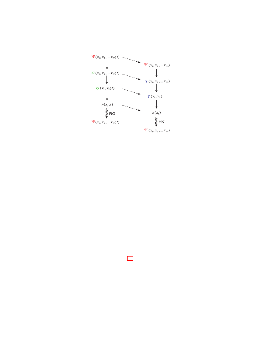
Figure 1:
Information on the time-and-space dependent wave func-
tion Ψ(x
1
, x
2
. . . , x
N
, t) is built into Green’s functions, and on the time-
independent wave function into density matrices. Integrating out degrees
of freedom reduces the N-particle Green’s function and N-particle density
matrix to the one-particle quantities G(x
1
, x
2
; t) and γ(x
1
, x
2
) described in
the main text. The diagonal element of the one-particle density matrix is
the ordinary charge density — the central quantity in DFT. The Hohenberg-
Kohn theorem and its time-dependent generalization (the Runge-Gross the-
orem) guarantee that the densities contain exactly the same information as
the wave functions.
via the so-called exchange-correlation functional. We will now see in some
detail how this is done.
4.1
Exchange-correlation energy: definition, interpre-
tation and exact properties
4.1.1
Exchange-correlation energy
The Thomas-Fermi approximation (34) for T [n] is not very good. A more
accurate scheme for treating the kinetic-energy functional of interacting elec-
trons, T [n], is based on decomposing it into one part that represents the ki-
netic energy of noninteracting particles of density n, i.e., the quantity called
above T
s
[n], and one that represents the remainder, denoted T
c
[n] (the sub-
26
scripts s and c stand for ‘single-particle’ and ‘correlation’, respectively).
T [n] = T
s
[n] + T
c
[n].
(53)
T
s
[n] is not known exactly as a functional of n [and using the LDA to ap-
proximate it leads one back to the Thomas-Fermi approximation (34)], but
it is easily expressed in terms of the single-particle orbitals φ
i
(r) of a nonin-
teracting system with density n, as
T
s
[n] = −
¯h
2
2m
N
X
i
Z
d
3
r φ
∗
i
(r)∇
2
φ
i
(r),
(54)
because for noninteracting particles the total kinetic energy is just the sum
of the individual kinetic energies. Since all φ
i
(r) are functionals of n, this
expression for T
s
is an explicit orbital functional but an implicit density
functional, T
s
[n] = T
s
[{φ
i
[n]}], where the notation indicates that T
s
depends
on the full set of occupied orbitals φ
i
, each of which is a functional of n.
Other such orbital functionals will be discussed in Sec. 5.
We now rewrite the exact energy functional as
E[n] = T [n] + U[n] + V [n] = T
s
[{φ
i
[n]}] + U
H
[n] + E
xc
[n] + V [n],
(55)
where by definition E
xc
contains the differences T − T
s
(i.e. T
c
) and U − U
H
.
This definition shows that a significant part of the correlation energy E
c
is due to the difference T
c
between the noninteracting and the interacting
kinetic energies. Unlike Eq. (35), Eq. (55) is formally exact, but of course
E
xc
is unknown — although the HK theorem guarantees that it is a density
functional. This functional, E
xc
[n], is called the exchange-correlation (xc)
energy. It is often decomposed as E
xc
= E
x
+ E
c
, where E
x
is due to the
Pauli principle (exchange energy) and E
c
is due to correlations. (T
c
is then
a part of E
c
.) The exchange energy can be written explicitly in terms of the
single-particle orbitals as
E
x
[{φ
i
[n]}] = −
q
2
2
P
jk
R
d
3
r
R
d
3
r
′ φ
∗
j
(r)φ
∗
k
(r
′
)φ
j
(r
′
)φ
k
(r)
|r−r
′
|
,
(56)
26
T
s
is defined as the expectation value of the kinetic-energy operator ˆ
T with the
Slater determinant arising from density n, i.e., T
s
[n] = hΦ[n]| ˆ
T |Φ[n]i. Similarly, the full
kinetic energy is defined as T [n] = hΨ[n]| ˆ
T |Ψ[n]i. All consequences of antisymmetrization
(i.e., exchange) are described by employing a determinantal wave function in defining T
s
.
Hence, T
c
, the difference between T
s
and T is a pure correlation effect.
27
This differs from the exchange energy used in Hartree-Fock theory only in the substi-
tution of Hartree-Fock orbitals φ
HF
i
(r) by Kohn-Sham orbitals φ
i
(r).
27

which is known as the Fock term, but no general exact expression in terms
of the density is known.
4.1.2
Different perspectives on the correlation energy
For the correlation energy no general explicit expression is known, neither in
terms of orbitals nor densities. Different ways to understand correlations are
described below.
Correlation energy: variational approach.
A simple way to understand
the origin of correlation is to recall that the Hartree energy is obtained in
a variational calculation in which the many-body wave function is approx-
imated as a product of single-particle orbitals. Use of an antisymmetrized
product (a Slater determinant) produces the Hartree and the exchange energy
[48, 49]. The correlation energy is then defined as the difference between the
full ground-state energy (obtained with the correct many-body wave func-
tion) and the one obtained from the (Hartree-Fock or Kohn-Sham
) Slater
determinant. Since it arises from a more general trial wave function than
a single Slater determinant, correlation cannot raise the total energy, and
E
c
[n] ≤ 0. Since a Slater determinant is itself more general than a simple
product we also have E
x
≤ 0, and thus the upper bound
E
xc
[n] ≤ 0.
Correlation energy: probabilistic approach.
Recalling the quantum me-
chanical interpretation of the wave function as a probability amplitude, we
see that a product form of the many-body wave function corresponds to treat-
ing the probability amplitude of the many-electron system as a product of
the probability amplitudes of individual electrons (the orbitals). Mathemat-
ically, the probability of a composed event is only equal to the probability
of the individual events if the individual events are independent (i.e., uncor-
related). Physically, this means that the electrons described by the product
wave function are independent.
Such wave functions thus neglect the fact
that, as a consequence of the Coulomb interaction, the electrons try to avoid
28
The Hartree-Fock and the Kohn-Sham Slater determinants are not identical, since
they are composed of different single-particle orbitals, and thus the definition of exchange
and correlation energy in DFT and in conventional quantum chemistry is slightly different
[52].
29
A lower bound is provided by the Lieb-Oxford formula, given in Eq. (64).
30
Correlation is a mathematical concept describing the fact that certain events are not
independent. It can be defined also in classical physics, and in applications of statistics
to other fields than physics. Exchange is due to the indistinguishability of particles, and
a true quantum phenomenon, without any analogue in classical physics.
28
each other. The correlation energy is simply the additional energy lowering
obtained in a real system due to the mutual avoidance of the interacting
electrons. One way to characterize a strongly correlated system is to define
correlations as strong when E
c
is comparable in magnitude to, or larger than,
other energy contributions, such as E
H
or T
s
. (In weakly correlated systems
E
c
normally is several orders of magnitude smaller.)
Correlation energy: beyond mean-field approach.
A rather different (but
equivalent) way to understand correlation is to consider the following alter-
native form of the operator representing the Coulomb interaction, equivalent
to Eq. (3),
ˆ
U =
q
2
2
Z
d
3
r
Z
d
3
r
′
ˆ
n(r)ˆ
n(r
′
) − ˆ
n(r)δ(r − r
′
)
|r − r
′
|
,
(57)
in which the operator character is carried only by the density operators ˆ
n
(in occupation number representation), and the term with the delta function
subtracts out the interaction of a charge with itself (cf., e.g., the appendix
of Ref. [53] for a simple derivation of this form of ˆ
U ). The expectation
value of this operator, U = hΨ| ˆ
U|Ψi, involves the expectation value of a
product of density operators, hΨ|ˆ
n(r)ˆ
n(r
′
)|Ψi. In the Hartree term (32),
on the other hand, this expectation value of a product is replaced by a
product of expectation values, each of the form n(r) = hΨ|ˆ
n(r)|Ψi. This
replacement amounts to a mean-field approximation, which neglects quantum
fluctuations
about the expectation values: by writing ˆ
n = n + δˆ
n
f luc
and
substituting in Eq. (57) we see that the difference between hΨ| ˆ
U|Ψi and
the Hartree term (32) is entirely due to the fluctuations δˆ
n
f luc
and the self-
interaction correction to the Hartree term. Quantum fluctuations about the
expectation value are thus at the origin of quantum correlations between
interacting particles.
31
Other characterizations of strongly correlated systems are to compare the width of the
conduction band in a solid with the kinetic energy (if the band width is smaller, correlations
are strong), or the quasiparticle energies ˜
ǫ
i
with the Kohn-Sham eigenvalues ǫ
i
(if both
are similar, correlations are weak, see footnote 37), or the derivative discontinuity ∆
xc
,
defined in Eq. (65), with the Kohn-Sham energy gap (if the former is comparable to or
larger than the latter, correlations are strong). (The meaning of ˜
ǫ
i
, ǫ
i
and ∆
xc
is explained
below.) No universally applicable definition of ‘strong correlations’ seems to exist.
32
At finite temperature there are also thermal fluctuations. To properly include these
one must use a finite-temperature formulation of DFT [54]. See also the contribution of
B. L. Gyorffy et al. in Ref. [19] for DFT treatment of various types of fluctuations.
29

Correlation energy: holes.
The fact that both exchange and correlation
tend to keep electrons apart, has given rise to the concept of an xc hole,
n
xc
(r, r
′
), describing the reduction of probability for encountering an elec-
tron at r
′
, given one at r. The xc energy can be written as a Hartree-like
interaction between the charge distribution n(r) and the xc hole n
xc
(r, r
′
) =
n
x
(r, r
′
) + n
c
(r, r
′
),
E
xc
[n] =
q
2
2
Z
d
3
r
Z
d
3
r
′
n(r)n
xc
(r, r
′
)
|r − r
′
|
,
(58)
which defines n
xc
. The exchange component E
x
[n] of the exact exchange-
correlation functional describes the energy lowering due to antisymmetriza-
tion (i.e., the tendency of like-spin electrons to avoid each other). It gives rise
to the exchange hole n
x
(r, r
′
), which obeys the sum rule
R
d
3
r
′
n
x
(r, r
′
) = −1.
The correlation component E
c
[n] accounts for the additional energy lower-
ing arising because electrons with opposite spins also avoid each other. The
resulting correlation hole integrates to zero, so that the total xc hole satis-
fies
R
d
3
r
′
n
xc
(r, r
′
) = −1. The xc hole can also be written as n
xc
(r, r
′
) =
n(r
′
)(¯
g[n](r, r
′
) − 1), where ¯
g is the average of the pair-correlation function
g(r, r
′
), mentioned in Sec. 3.5.2, over all values of the particle-particle interac-
tion, from zero (KS system) to h ˆ
Ui (interacting system). This average is sim-
ply expressed in terms of the coupling constant α as ¯
g(r, r
′
) =
R
1
0
g
α
(r, r
′
)dα.
For the Coulomb interaction, α = e
2
, i.e., the square of the electron charge
4.1.3
Exact properties
Clearly E
c
is an enormously complex object, and DFT would be of little use if
one had to know it exactly for making calculations. The practical advantage
of writing E[n] in the form Eq. (55) is that the unknown functional E
xc
[n] is
typically much smaller than the known terms T
s
, U
H
and V . One can thus
hope that reasonably simple approximations for E
xc
[n] provide useful results
for E[n]. Some successful approximations are discussed in Sec. 5. Exact prop-
erties, such as the sum rule
R
d
3
r
′
n
xc
(r, r
′
) = −1, described in the preceding
section, are most valuable guides in the construction of approximations to
E
xc
[n].
Among the known properties of this functional are the coordinate scaling
conditions first obtained by Levy and Perdew [55]
E
x
[n
λ
] = λE
x
[n]
(59)
30

E
c
[n
λ
] > λE
c
[n]
for λ > 1
(60)
E
c
[n
λ
] < λE
c
[n]
for λ < 1,
(61)
where n
λ
(r) = λ
3
n(λr) is a scaled density integrating to total particle number
N.
Another important property of the exact functional is the one-electron
limit
E
c
[n
(1)
] ≡ 0
(62)
E
x
[n
(1)
] ≡ −E
H
[n
(1)
],
(63)
where n
(1)
is a one-electron density. These latter two conditions, which are
satisfied within the Hartree-Fock approximation, but not by standard local-
density and gradient-dependent functionals, ensure that there is no artificial
self-interaction of one electron with itself.
The Lieb-Oxford bound [56, 57],
E
x
[n] ≥ E
xc
[n] ≥ −1.68e
2
Z
d
3
r n(r)
4/3
,
(64)
establishes a lower bound on the xc energy, and is satisfied by LDA and many
(but not all) GGAs.
One of the most intriguing properties of the exact functional, which has
resisted all attempts of describing it in local or semilocal approximations,
is the derivative discontinuity of the xc functional with respect to the total
particle number [50, 58, 59],
δE
xc
[n]
δn(r)
N +δ
−
δE
xc
[n]
δn(r)
N −δ
= v
+
xc
(r) − v
−
xc
(r) = ∆
xc
,
(65)
where δ is an infinitesimal shift of the electron number N, and ∆
xc
is a
system-dependent, but r-independent shift of the xc potential v
xc
(r) as it
passes from the electron-poor to the electron-rich side of integer N. The
noninteracting kinetic-energy functional has a similar discontinuity, given by
δT
s
[n]
δn(r)
N +δ
−
δT
s
[n]
δn(r)
N −δ
= ǫ
N +1
− ǫ
N
= ∆
KS
,
(66)
where ǫ
N
and ǫ
N +1
are the Kohn-Sham (KS) single-particle energies of the
highest occupied and lowest unoccupied eigenstate. The meaning of these
31
KS eigenvalues is discussed in the paragraphs following Eq. (75) and illus-
trated in Fig. 2. In the chemistry literature these are called the HOMO
(highest occupied molecular orbital) and LUMO (lowest unoccupied molec-
ular orbital), respectively.
The kinetic-energy discontinuity is thus sim-
ply the KS single-particle gap ∆
KS
, or HOMO-LUMO gap, whereas the
xc discontinuity ∆
xc
is a many-body effect.
The true fundamental gap
∆ = E(N + 1) + E(N − 1) − 2E(N) is the discontinuity of the total ground-
state energy functional [5, 50, 58, 59],
∆ =
δE[n]
δn(r)
N +δ
−
δE[n]
δn(r)
N −δ
= ∆
KS
+ ∆
xc
.
(67)
Since all terms in E other than E
xc
and T
s
are continuous functionals of
n(r), the fundamental gap is the sum of the KS gap and the xc discontinuity.
Standard density functionals (LDA and GGA) predict ∆
xc
= 0, and thus
often underestimate the fundamental gap. The fundamental and KS gaps
are also illustrated in Fig. 2.
All these properties serve as constraints or guides in the construction of
approximations for the functionals E
x
[n] and E
c
[n]. Many other similar prop-
erties are known. A useful overview of scaling properties is the contribution
of M. Levy in Ref. [19].
4.2
Kohn-Sham equations
4.2.1
Derivation of the Kohn-Sham equations
Since T
s
is now written as an orbital functional one cannot directly minimize
Eq. (55) with respect to n. Instead, one commonly employs a scheme sug-
gested by Kohn and Sham [60] for performing the minimization indirectly.
This scheme starts by writing the minimization as
0 =
δE[n]
δn(r)
=
δT
s
[n]
δn(r)
+
δV [n]
δn(r)
+
δU
H
[n]
δn(r)
+
δE
xc
[n]
δn(r)
=
δT
s
[n]
δn(r)
+v(r)+v
H
(r)+v
xc
(r).
(68)
As a consequence of Eq. (27), δV /δn = v(r), the ‘external’ potential the
electrons move in.
The term δU
H
/δn simply yields the Hartree potential,
33
This potential is called ‘external’ because it is external to the electron system and
not generated self-consistently from the electron-electron interaction, as v
H
and v
xc
. It
comprises the lattice potential and any additional truly external field applied to the system
as a whole.
32

introduced in Eq. (11). For the term δE
xc
/δn, which can only be calculated
explicitly once an approximation for E
xc
has been chosen, one commonly
writes v
xc
. By means of the Sham-Schl¨
uter equation (39), v
xc
is related to
the irreducible self energy Σ, introduced in Eq. (38) [50].
Consider now a system of noninteracting particles moving in the potential
v
s
(r). For this system the minimization condition is simply
0 =
δE
s
[n]
δn(r)
=
δT
s
[n]
δn(r)
+
δV
s
[n]
δn(r)
=
δT
s
[n]
δn(r)
+ v
s
(r),
(69)
since there are no Hartree and xc terms in the absence of interactions. The
density solving this Euler equation is n
s
(r). Comparing this with Eq. (68)
we find that both minimizations have the same solution n
s
(r) ≡ n(r), if v
s
is chosen to be
v
s
(r) = v(r) + v
H
(r) + v
xc
(r).
(70)
Consequently, one can calculate the density of the interacting (many-body)
system in potential v(r), described by a many-body Schr¨odinger equation
of the form (2), by solving the equations of a noninteracting (single-body)
system in potential v
s
(r).
In particular, the Schr¨odinger equation of this auxiliary system,
h
−
¯
h
2
∇
2
2m
+ v
s
(r)
i
φ
i
(r) = ǫ
i
φ
i
(r),
(71)
yields orbitals that reproduce the density n(r) of the original system (these
are the same orbitals employed in Eq. (54)),
n(r) ≡ n
s
(r) =
P
N
i
f
i
|φ
i
(r)|
2
,
(72)
where f
i
is the occupation of the i’th orbital.
celebrated Kohn-Sham (KS) equations. They replace the problem of mini-
mizing E[n] by that of solving a noninteracting Schr¨odinger equation. (Recall
34
The question whether such a potential v
s
(r) always exists in the mathematical sense
is called the noninteracting v-representability problem. It is known that every interacting
ensemble v-representable density is also noninteracting ensemble v-representable, but, as
mentioned in Sec. 3.2, only in discretized systems has it been proven that all densities are
interacting ensemble v-representable. It is not known if interacting ensemble-representable
densities may be noninteracting pure-state representable (i.e, by a single determinant),
which would be convenient (but is not necessary) for Kohn-Sham calculations.
35
Normally, the occupation numbers f
i
follows an Aufbau principle (Fermi statistics)
with f
i
= 1 for i < N , f
i
= 0 for i > N , and 0 ≤ f
i
≤ 1 for i = N (i.e., at most
33
that the minimization of E[n] originally replaced the problem of solving the
many-body Schr¨odinger equation!)
Since both v
H
and v
xc
depend on n, which depends on the φ
i
, which in
turn depend on v
s
, the problem of solving the KS equations is a nonlinear
one, just as is the one of solving the (much more complicated) Dyson equation
(38). The usual way of solving such problems is to start with an initial guess
for n(r), calculate the corresponding v
s
(r), and then solve the differential
equation (71) for the φ
i
. From these one calculates a new density, using (72),
and starts again. The process is repeated until it converges. The technical
name for this procedure is ‘self-consistency cycle’. Different convergence
criteria (such as convergence in the energy, the density, or some observable
calculated from these) and various convergence-accelerating algorithms (such
as mixing of old and new effective potentials) are in common use. Only rarely
it requires more than a few dozen iterations to achieve convergence, and even
rarer are cases where convergence seems unattainable, i.e., a self-consistent
solution of the KS equation cannot be found.
Once one has a converged solution n
0
, one can calculate the total energy
from Eq. (55) or, equivalently and more conveniently, from
E
0
=
P
N
i
ǫ
i
−
q
2
2
R
d
3
r
R
d
3
r
′ n
0
(r)n
0
(r
′
)
|r−r
′
|
−
R
d
3
r v
xc
(r)n
0
(r) + E
xc
[n
0
].
(73)
Equation (73) follows from writing V [n] in (55) by means of (70) as
V [n] =
Z
d
3
r v(r)n(r) =
Z
d
3
r [v
s
(r) − v
H
(r) − v
xc
(r)]n(r)
(74)
= V
s
[n] −
Z
d
3
r [v
H
(r) + v
xc
(r)]n(r),
(75)
the highest occupied orbital can have fractional occupation). Some densities that are not
noninteracting v-representable by a single ground-state Slater determinant, may still be
obtained from a single determinant if one uses occupation numbers f
i
that leave holes
below the HOMO (the Fermi energy in a metal), so that f
i
6= 1 even for some i < N
[31], but this is not guaranteed to describe all possible densities. Alternatively (see Sec.
3.2 and footnote 34) a Kohn-Sham equation may be set up in terms of ensembles of
determinants. This guarantees noninteracting v-representability for all densities that are
interacting ensemble v-representable. For practical KS calculations, the most important
consequence of the fact that not every arbitrary density is guaranteed to be noninteracting
v-representable is that the Kohn-Sham selfconsistency cycle is not guaranteed to converge.
36
All terms on the right-hand side of (73) except for the first, involving the sum of the
single-particle energies, are sometimes known as double-counting corrections, in analogy
to a similar equation valid within Hartree-Fock theory.
34

and identifying the energy of the noninteracting (Kohn-Sham) system as
E
s
=
P
N
i
ǫ
i
= T
s
+ V
s
.
4.2.2
The eigenvalues of the Kohn-Sham equation
Equation (73) shows that E
0
is not simply the sum
of all ǫ
i
. In fact, it
should be clear from our derivation of Eq. (71) that the ǫ
i
are introduced as
completely artificial objects: they are the eigenvalues of an auxiliary single-
body equation whose eigenfunctions (orbitals) yield the correct density. It is
only this density that has strict physical meaning in the KS equations. The
KS eigenvalues, on the other hand, in general bear only a semiquantitative
resemblance with the true energy spectrum [61], but are not to be trusted
quantitatively.
The main exception to this rule is the highest occupied KS eigenvalue.
Denoting by ǫ
N
(M) the N’th eigenvalue of a system with M electrons, one
can show rigorously that ǫ
N
(N) = −I, the negative of the first ionization
energy of the N-body system, and ǫ
N +1
(N + 1) = −A, the negative of the
electron affinity of the same N-body system [58, 62, 63]. These relations
hold for the exact functional only. When calculated with an approximate
functional of the LDA or GGA type, the highest eigenvalues usually do not
provide good approximations to the experimental I and A. Better results
for these observables are obtained by calculating them as total-energy differ-
ences, according to I = E
0
(N − 1) − E
0
(N) and A = E
0
(N) − E
0
(N + 1),
where E
0
(N) is the ground-state energy of the N-body system. Alterna-
tively, self-interaction corrections can be used to obtain improved ionization
energies and electron affinities from Kohn-Sham eigenvalues [64].
Figure 2 illustrates the role played by the highest occupied and lowest
unoccupied KS eigenvalues, and their relation to observables. For molecules,
HOMO(N) is the highest-occupied molecular orbital of the N-electron sys-
tem, HOMO(N+1) that of the N + 1-electron system, and LUMO(N) the
lowest unoccupied orbital of the N-electron system. In solids with a gap,
37
The difference between E
0
and
P
N
i
ǫ
i
is due to particle-particle interactions. The ad-
ditional terms on the right-hand side of (73) give mathematical meaning to the common
statement that the whole is more than the sum of its parts. If E
0
can be written approx-
imately as
P
N
i
˜
ǫ
i
(where the ˜
ǫ
i
are not the same as the KS eigenvalues ǫ
i
) the system
can be described in terms of N weakly interacting quasiparticles, each with energy ˜
ǫ
i
.
Fermi-liquid theory in metals and effective-mass theory in semiconductors are examples
of this type of approach.
35
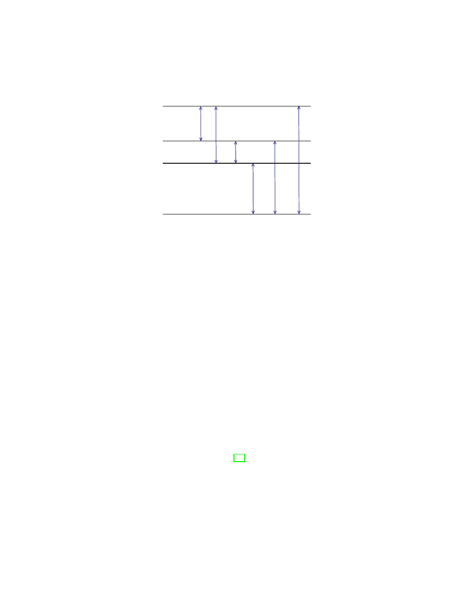
A
KS
A
KS
D
xc
D
D
I
)
(N
LUMO
)
1
( +
N
HOMO
0
)
(N
HOMO
Figure 2: Schematic description of some important Kohn-Sham eigenvalues
relative to the vacuum level, denoted by 0, and their relation to observables.
See main text for explanations.
the HOMO and LUMO become the top of the valence band and the bottom
of the conduction band, respectively, whereas in metals they are both iden-
tical to the Fermi level. The vertical lines indicate the Kohn-Sham (single-
particle) gap ∆
KS
, the fundamental (many-body) gap ∆, the derivative dis-
continuity of the xc functional, ∆
xc
, the ionization energy of the interacting
N-electron system I(N) = −ǫ
N
(N) (which is also the ionization energy of
the Kohn-Sham system I
KS
(N)), the electron affinity of the interacting N-
electron system A(N) = −ǫ
N +1
(N + 1) and the Kohn-Sham electron affinity
A
KS
(N) = −ǫ
N +1
(N).
Given the auxiliary nature of the other Kohn-Sham eigenvalues, it comes
as a great (and welcome) surprise that in many situations (typically char-
acterized by the presence of fermionic quasiparticles and absence of strong
correlations) the Kohn-Sham eigenvalues ǫ
i
do, empirically, provide a rea-
sonable first approximation to the actual energy levels of extended systems.
This approximation is behind most band-structure calculations in solid-state
physics, and often gives results that agree well with experimental photoemis-
sion and inverse photoemission data [65], but much research remains to be
done before it is clear to what extent such conclusions can be generalized,
and how situations in which the KS eigenvalues are good starting points for
approximating the true excitation spectrum are to be characterized micro-
36
Most band-structure calculations in solid-state physics are actually calcu-
lations of the KS eigenvalues ǫ
i
This simplification has proved enormously
successful, but when one uses it one must be aware of the fact that one is
taking the auxiliary single-body equation (71) literally as an approximation
to the many-body Schr¨odinger equation. DFT, practiced in this mode, is not
a rigorous many-body theory anymore, but a mean-field theory (albeit one
with a very sophisticated mean field v
s
(r)).
The energy gap obtained in such band-structure calculations is the one
called HOMO-LUMO gap in molecular calculations, i.e., the difference be-
tween the energies of the highest occupied and the lowest unoccupied single-
particle states. Neglect of the derivative discontinuity ∆
xc
, defined in Eq. (65),
by standard local and semilocal xc functionals leads to an underestimate of
the gap (the so-called ‘band-gap problem’), which is most severe in transition-
metal oxides and other strongly correlated systems. Self-interaction correc-
tions provide a partial remedy for this problem [71, 72, 73, 74].
4.2.3
Hartree, Hartree-Fock and Dyson equations
A partial justification for the interpretation of the KS eigenvalues as start-
ing point for approximations to quasi-particle energies, common in band-
structure calculations, can be given by comparing the KS equation with
other self-consistent equations of many-body physics. Among the simplest
such equations are the Hartree equation
"
−
¯h
2
∇
2
2m
+ v(r) + v
H
(r)
#
φ
H
i
(r) = ǫ
H
i
φ
H
i
(r),
(76)
and the Hartree-Fock (HF) equation
"
−
¯h
2
∇
2
2m
+ v(r) + v
H
(r)
#
φ
HF
i
(r) − q
2
Z
d
3
r
′
γ(r, r
′
)
|r − r
′
|
φ
HF
i
(r
′
) = ǫ
HF
i
φ
HF
i
(r),
(77)
where γ(r, r
′
) is the density matrix of Eq. (46). It is a fact known as Koop-
man’s theorem [49] that the HF eigenvalues ǫ
HF
i
can be interpreted as unre-
laxed electron-removal energies (i.e., ionization energies of the i’th electron,
38
Several more rigorous approaches to excited states in DFT, which do not require the
KS eigenvalues to have physical meaning, are mentioned in Sec. 6.
39
A computationally more expensive, but more reliable, alternative is provided by the
GW approximation [68, 69, 70].
37
neglecting reorganization of the remaining electrons after removal). As men-
tioned above, in DFT only the highest occupied eigenvalue corresponds to
an ionization energy, but unlike in HF this energy includes relaxation effects.
The KS equation (71) includes both exchange and correlation via the
multiplicative operator v
xc
. Both exchange and correlation are normally
approximated in DFT,
whereas HF accounts for exchange exactly, through
the integral operator containing γ(r, r
′
), but neglects correlation completely.
In practise DFT results are typically at least as good as HF ones and often
comparable to much more sophisticated correlated methods — and the KS
equations are much easier to solve than the HF equations.
All three single-particle equations, Hartree, Hartree-Fock and Kohn-Sham
can also be interpreted as approximations to Dyson’s equation (38), which
can be rewritten as [48]
−
¯h
2
∇
2
2m
+ v(r)
!
ψ
k
(r) +
Z
d
3
r
′
Σ(r, r
′
, E
k
)ψ
k
(r
′
) = E
k
ψ
k
(r),
(78)
where Σ is the irreducible self energy introduced in Eq. (38). The E
k
ap-
pearing in this equation are the true (quasi-)electron addition and removal
energies of the many-body system. Needless to say, it is much more compli-
cated to solve this equation than the HF or KS equations. It is also much
harder to find useful approximations for Σ than for v
xc
Obviously, the KS
equation employs a local, energy-independent potential v
s
in place of the non-
local, energy-dependent operator Σ. Whenever this is a good approximation,
the ǫ
i
are also a good approximation to the E
k
.
The interpretation of the KS equation (71) as an approximation to Eq. (78)
is suggestive and useful, but certainly not necessary for DFT to work: if the
KS equations are only used to obtain the density, and all other observables,
such as total energies, are calculated from this density, then the KS equa-
tions in themselves are not an approximation at all, but simply a very useful
mathematical tool.
40
A possibility to treat exchange exactly in DFT is offered by the OEP method discussed
in Sec. 5.3.
41
This is due to the integral operator in the HF equations.
42
The GW approximation [68, 69, 70], mentioned in footnote 39, is one such approxi-
mation for Σ, but in actual implementations of it one usually takes DFT-KS results as an
input.
38

4.3
Basis functions
In practice, numerical solution of the KS differential equation (71) typically
proceeds by expanding the KS orbitals in a suitable set of basis functions and
solving the resulting secular equation for the coefficients in this expansion
and/or for the eigenvalues for which it has a solution. The construction
of suitable basis functions is a major enterprise within electronic-structure
theory (with relevance far beyond DFT), and the following lines do little
more than explaining some acronyms often used in this field.
In physics much is known about the construction of basis functions for
solids due to decades of experience with band-structure calculations. This in-
cludes many calculations that predate the widespread use of DFT in physics.
There is a fundamental dichotomy between methods that work with fixed ba-
sis functions that do not depend on energy, and methods that employ energy-
dependent basis functions. Fixed basis functions are used e.g., in plane-wave
expansions, tight-binding or LCAO (linear combination of atomic orbitals)
approximations, or the OPW (orthogonalized plane wave) method. Exam-
ples for methods using energy-dependent functions are the APW (augmented
plane wave) or KKR (Korringa-Kohn-Rostoker) approaches. This distinction
became less clear-cut with the introduction of ‘linear methods’ [75], in which
energy-dependent basis functions are linearized (Taylor expanded) around
some fixed reference energy. The most widely used methods for solving the
Kohn-Sham equation in solid-state physics, LMTO (linear muffin tin or-
bitals) and LAPW (linear augmented plane waves), are of this latter type
[76]. Development of better basis functions is an ongoing enterprise [77, 78].
The situation is quite similar in chemistry. Due to decades of experience
with Hartree-Fock and CI calculations much is known about the construction
of basis functions that are suitable for molecules. Almost all of this continues
to hold in DFT — a fact that has greatly contributed to the recent popularity
of DFT in chemistry. Chemical basis functions are classified with respect
to their behaviour as a function of the radial coordinate into Slater type
orbitals (STOs), which decay exponentially far from the origin, and Gaussian
type orbitals (GTOs), which have a gaussian behaviour. STOs more closely
resemble the true behaviour of atomic wave functions [in particular the cusp
condition of Eq. (19)], but GTOs are easier to handle numerically because
the product of two GTOs located at different atoms is another GTO located
in between, whereas the product of two STOs is not an STO. The so-called
‘contracted basis functions’, in which STO basis functions are reexpanded in
39

a small number of GTOs, represent a compromise between the accuracy of
STOs and the convenience of GTOs. The most common methods for solving
the Kohn-Sham equations in quantum chemistry are of this type [4, 49].
Very accurate basis functions for chemical purposes have been constructed
by Dunning [79] and, more recently, by da Silva and collaborators [80, 81].
More details on the development of suitable basis functions can be found,
e.g., in these references and Ref. [49].
A very popular approach to larger systems in DFT, in particular solids,
is based on the concept of a pseudopotential (PP). The idea behind the PP
is that chemical binding in molecules and solids is dominated by the outer
(valence) electrons of each atom. The inner (core) electrons retain, to a good
approximation, an atomic-like configuration, and their orbitals do not change
much if the atom is put in a different environment. Hence, it is possible to
approximately account for the core electrons in a solid or a large molecule
by means of an atomic calculation, leaving only the valence density to be
determined self-consistently for the system of interest.
In the original Kohn-Sham equation the effective potential v
s
[n] = v
ext
+
v
H
[n] + v
xc
[n] is determined by the full electronic density n(r), and the self-
consistent solutions are single-particle orbitals reproducing this density. In
the PP approach the Hartree and xc terms in v
s
[n] are evaluated only for
the valence density n
v
, and the core electrons are accounted for by replac-
ing the external potential v
ext
by a pseudopotential v
P P
ext
. Hence v
P P
s
[n
v
] =
v
P P
ext
+ v
H
[n
v
] + v
xc
[n
v
].
The PP v
P P
ext
is determined in two steps. First, one
determines, in an auxiliary atomic calculation, an effective PP, v
P P
s
, such
that for a suitably chosen atomic reference configuration the single-particle
orbitals resulting from v
P P
s
agree — outside a cut-off radius r
c
separating the
core from the valence region — with the valence orbitals obtained from the
all-electron KS equation for the same atom. As a consequence, the valence
densities n
at
v
obtained from the atomic KS and the atomic PP equation are
the same. Next, one subtracts the atomic valence contributions v
H
[n
at
v
] and
v
xc
[n
at
v
] from v
P P
s
[n
at
v
] to obtain the external PP v
P P
ext
which is then used
43
Note that the effective potential v
s
is a way to deal with the electron-electron inter-
action. The pseudopotential is a way to deal with the density of the core electrons. Both
potentials can be profitably used together, but are conceptually different.
44
This external PP is also called the unscreened PP, and the subtraction of v
H
[n
at
v
] and
v
xc
[n
at
v
] from v
P P
s
[n
at
v
] is called the ’unscreening of the atomic PP’. It can only be done
exactly for the Hartree term, because the contributions of valence and core densities are
not additive in the xc potential (which is a nonlinear functional of the total density).
40
in the molecular or solid-state calculation, together with v
H
[n
v
] and v
xc
[n
v
]
taken at the proper valence densities for these systems.
The way v
P P
s
is generated from the atomic calculation is not unique.
Common pseudopotentials are generated following the prescription of, e.g.,
Bachelet, Hamann and Schl¨
uter [82], Kleinman and Bylander [83], Vanderbilt
[84] or Troullier and Martins [85]. Useful reviews are Refs. [86, 87, 88]. The
pseudopotential approach is very convenient because it reduces the number of
electrons treated explicitly, making it possible to perform density-functional
calculations on systems with tens of thousands of electrons. Moreover, the
pseudopotentials v
P P
ext
are much smoother than the bare nuclear potentials
v
ext
. The remaining valence electrons are thus well described by plane-wave
basis sets.
Some of the choices one has to make in a practical Kohn-Sham calculation
are illustrated schematically in Fig. 3.
5
Making DFT practical: Approximations
There are basically three distinct types of approximations involved in
a DFT calculation. One is conceptual, and concerns the interpretation of
KS eigenvalues and orbitals as physical energies and wave functions. This
approximation is optional — if one does not want to make it one simply
does not attach meaning to the eigenvalues of Eq. (71). The pros and cons
of this procedure were discussed in Secs. 4.2.2 and 4.2.3. The second type
of approximation is numerical, and concerns methods for actually solving
the differential equation (71). A main aspect here is the selection of suitable
basis functions, briefly discussed in Sec. 4.3. The third type of approximation
involves constructing an expression for the unknown xc functional E
xc
[n],
which contains all many-body aspects of the problem [cf. Eq. (55)]. It is
with this type of approximation that we are concerned in the present section.
This chapter is intended to give the reader an idea of what types of
functionals exist, and to describe what their main features are, separately
for local functionals (TF, LDA and Xα; Sec. 5.1), semilocal, or gradient-
dependent, functionals (GEA and GGA; Sec. 5.2), and nonlocal functionals
(hybrids, orbital functionals such as meta-GGAs, EXX and SIC, and integral-
dependent functionals such as ADA; Sec. 5.3). This chapter does deal only
most superficially with the actual construction of these functionals. For more
41
)
(
)
(
)
(
)
(
)
(
2
2
r
r
r
r
r
n
n
n
xc
H
ext
v
v
v
m
f
e
f
=
ú
û
ù
ê
ë
é
+
+
+
Ñ
-
non relativistic: Schrödinger
scalar relativistic
relativistic: Dirac
L(S)DA
GGA
hybrids
MGGA
Lagrange multipliers
band structure
nuclei
pseudopotential
Poisson eq.
integral
mesh/basis
GTO/STO/...
LMTO/LAPW/PW/...
Figure 3: Some of the choices made in a Kohn-Sham calculation. The treat-
ment can be nonrelativistic (based on Schr¨odinger’s equation), scalar rela-
tivistic (using the relativistic kinetic-energy operator and other simple rela-
tivistic corrections, but no spin-orbit coupling) or relativistic (using Dirac’s
equation, which includes also spin-orbit coupling). The core electrons can
be treated explicitly (all electron calculation) or incorporated, together with
v
ext
, in a pseudopotential. The Hartree potential can be obtained from in-
tegrating the charge density or from solving Poisson’s differential equation.
Many choices are available for the xc potential. The eigenvalues can be
considered mere Lagrange multipliers or interpreted as zero-order approxi-
mations to the actual energy spectrum. The eigenfunctions can similarly be
considered auxiliary functions generating the density, or interpreted as zero-
order approximations to quasi-particle wave functions. Solution of the KS
equation can proceed on a numerical mesh, or by expansion of the eigenfunc-
tions in basis functions. Many types of suitable basis functions exist. For
every new problem a suitable combination of choices must be made, and all
possibilities continue to be useful and to be actively explored in physics and
chemistry.
42

details on functional construction and testing the reader is referred to the
reviews [5-19] or to the original papers cited below. Sticking to the bird’s-eye
philosophy of this overview I have also refrained from including numerical
data on the performance of each functional — extensive comparisons of a
wide variety of functionals can be found in Refs. [5-19] and in the original
literature cited below.
5.1
Local functionals: LDA
Historically (and in many applications also practically) the most important
type of approximation is the local-density approximation (LDA). To under-
stand the concept of an LDA recall first how the noninteracting kinetic en-
ergy T
s
[n] is treated in the Thomas-Fermi approximation: In a homogeneous
system one knows that, per volume
t
hom
s
(n) =
3¯h
2
10m
(3π
2
)
2/3
n
5/3
(79)
where n = const. In an inhomogeneous system, with n = n(r), one approxi-
mates locally
t
s
(r) ≈ t
hom
s
(n(r)) =
3¯h
2
10m
(3π
2
)
2/3
n(r)
5/3
(80)
and obtains the full kinetic energy by integration over all space
T
LDA
s
[n] =
Z
d
3
r t
hom
s
(n(r)) =
3¯h
2
10m
(3π
2
)
2/3
Z
d
3
r n(r)
5/3
.
(81)
For the kinetic energy the approximation T
s
[n] ≈ T
LDA
s
[n] is much inferior
to the exact treatment of T
s
in terms of orbitals, offered by the Kohn-Sham
equations, but the LDA concept turned out to be highly useful for another
component of the total energy (55), the exchange-correlation energy E
xc
[n].
For the exchange energy E
x
[n] the procedure is very simple, since the per-
volume exchange energy of the homogeneous electron liquid is known exactly
[5, 6],
e
hom
x
(n) = −
3q
2
4
3
π
1/3
n
4/3
,
(82)
45
The change from a capital T to a lower-case t is commonly used to indicate quantities
per volume.
43
so that
E
LDA
x
[n] = −
3q
2
4
3
π
1/3
R
d
3
r n(r)
4/3
.
(83)
This is the LDA for E
x
For the correlation energy E
c
[n] the situation is more complicated since
e
hom
c
(n) is not known exactly: the determination of the correlation energy
of a homogeneous interacting electron system (an electron liquid) is already
a difficult many-body problem on its own! Early approximate expressions
for e
hom
c
(n) were based on applying perturbation theory (e.g. the random-
phase approximation) to this problem [89, 90]. These approximations became
outdated with the advent of highly precise Quantum Monte Carlo (QMC)
calculations for the electron liquid, by Ceperley and Alder [91]. Modern
expressions for e
hom
c
(n) [92, 93, 94] are parametrizations of these data. These
expressions are implemented in most standard DFT program packages and
in typical applications give almost identical results. On the other hand, the
earlier parametrizations of the LDA, based on perturbation theory [89, 90],
can occasionally deviate substantially from the QMC ones, and are better
avoided.
Independently of the parametrization, the LDA for E
xc
[n] formally con-
sists in
E
xc
[n] ≈ E
LDA
xc
[n] =
R
d
3
r e
hom
xc
(n)|
n→n(r)
=
R
d
3
r e
hom
xc
(n(r)),
(84)
where e
hom
xc
= e
hom
x
+ e
hom
c
. The corresponding xc potential is simply
v
LDA
xc
[n](r) =
∂e
hom
xc
(n)
∂n
n→n(r)
.
(85)
This approximation for E
xc
[n] has proved amazingly successful, even when
applied to systems that are quite different from the electron liquid that forms
the reference system for the LDA. A partial explanation for this success of the
46
If one adds this term to the Thomas-Fermi expression (35) one obtains the so-called
Thomas-Fermi-Dirac approximation to E[n]. It one multiplies it with an adjustable pa-
rameter α one obtains the so-called Xα approximation to E
xc
[n]. These approximations
are not much used today in DFT.
47
Sometimes one uses the per-particle instead of the per-volume energy of the homoge-
neous system in writing the LDA. Since the conversion factor between both is the number
of particles per volume, i.e., the density, an additional n(r) then appears under the inte-
grals in (84) and also contributes to (85).
44

LDA is systematic error cancellation: typically, LDA underestimates E
c
but
overestimates E
x
, resulting in unexpectedly good values of E
xc
. This error
cancellation is not accidental, but systematic, and caused by the fact that for
any density the LDA xc hole satisfies the correct sum rule
R
d
3
r
′
n
LDA
xc
(r, r
′
) =
−1 (see Sec. 4.1.2), which is only possible if integrated errors in n
LDA
x
cancel
with those of n
LDA
c
.
For many decades the LDA has been applied in, e.g., calculations of band
structures and total energies in solid-state physics. In quantum chemistry
it is much less popular, because it fails to provide results that are accurate
enough to permit a quantitative discussion of the chemical bond in molecules
(so-called ‘chemical accuracy’ requires calculations with an error of not more
than about 1 kcal/mol = 0.04336 eV/particle).
At this stage it may be worthwhile to recapitulate what practical DFT
does, and where the LDA enters its conceptual structure: What real systems,
such as atoms, molecules, clusters and solids, have in common, is that they
are simultaneously inhomogeneous (the electrons are exposed to spatially
varying electric fields produced by the nuclei) and interacting (the electrons
interact via the Coulomb interaction). The way density-functional theory, in
the local-density approximation, deals with this inhomogeneous many-body
problem is by decomposing it into two simpler (but still highly nontrivial)
problems: the solution of a spatially homogeneous interacting problem (the
homogeneous electron liquid) yields the uniform xc energy e
hom
xc
(n), and the
solution of a spatially inhomogeneous noninteracting problem (the inhomoge-
neous electron gas described by the KS equations) yields the particle density.
Both steps are connected by the local-density potential (85), which shows how
the xc energy of the uniform interacting system enters the equations for the
inhomogeneous noninteracting system.
The particular way in which the inhomogeneous many-body problem is
decomposed, and the various possible improvements on the LDA, are behind
the success of DFT in practical applications of quantum mechanics to real
materials. Some such improvements on the LDA are discussed in the next
two sections.
5.2
Semilocal functionals: GEA, GGA and beyond
In the LDA one exploits knowledge of the density at point r. Any real system
is spatially inhomogeneous, i.e., it has a spatially varying density n(r), and
it would clearly be useful to also include information on the rate of this
45

variation in the functional. A first attempt at doing this were the so-called
‘gradient-expansion approximations’ (GEA). In this class of approximation
one tries to systematically calculate gradient-corrections of the form |∇n(r)|,
|∇n(r)|
2
, ∇
2
n(r), etc., to the LDA. A famous example is the lowest-order
gradient correction to the Thomas-Fermi approximation for T
s
[n],
T
s
[n] ≈ T
W
s
[n] = T
LDA
s
[n] +
¯h
2
8m
Z
d
3
r
|∇n(r)|
2
n(r)
.
(86)
This second term on the right-hand side is called the Weizs¨acker term.
Similarly, in
E
x
[n] ≈ E
GEA(2)
x
[n] = E
LDA
x
[n] −
10q
2
432π(3π
2
)
1/3
Z
d
3
r
|∇n(r)|
2
n(r)
4/3
(87)
the second term on the right-hand side is the lowest-order gradient correc-
tion
to E
LDA
x
[n]. In practice, the inclusion of low-order gradient corrections
almost never improves on the LDA, and often even worsens it. Higher-order
corrections (e.g., ∝ |∇n(r)|
α
or ∝ ∇
β
n(r) with α, β > 2), on the other hand,
are exceedingly difficult to calculate, and little is known about them.
In this situation it was a major breakthrough when it was realized, in the
early eighties, that instead of power-series-like systematic gradient expan-
sions one could experiment with more general functions of n(r) and ∇n(r),
which need not proceed order by order. Such functionals, of the general form
E
GGA
xc
[n] =
Z
d
3
r f (n(r), ∇n(r)),
(88)
have become known as generalized-gradient approximations (GGAs) [95].
Different GGAs differ in the choice of the function f (n, ∇n). Note that
this makes different GGAs much more different from each other than the
different parametrizations of the LDA: essentially there is only one correct
48
If one adds this term to the Thomas-Fermi expression (35) one obtains the so-called
Thomas-Fermi-Weizs¨
acker approximation to E[n]. In a systematic gradient expansion the
8 in the denominator is replaced by a 72 [5, 6].
49
Remarkably, the form of this term is fully determined already by dimensional analysis:
In E
GEA(2)
x
= q
2
R d
3
r f (n, |∇n|
2
) the function f must have dimensions (length)
−
4
. Since
the dimensions of n and |∇n|
2
are (length)
−
3
and (length)
−
8
, respectively, and to second
order no higher powers or higher derivatives of n are allowed, the only possible combination
is f ∝ |∇n(r)|
2
/n
4/3
.
46
expression for e
hom
xc
(n), and the various parametrizations of the LDA [89,
90, 92, 93, 94] are merely different ways of writing it. On the other hand,
depending on the method of construction employed for obtaining f (n, ∇n)
one can obtain very different GGAs. In particular, GGAs used in quantum
chemistry typically proceed by fitting parameters to test sets of selected
molecules. On the other hand, GGAs used in physics tend to emphasize
exact constraints. Nowadays the most popular (and most reliable) GGAs
are PBE (denoting the functional proposed in 1996 by Perdew, Burke and
Ernzerhof [96]) in physics, and BLYP (denoting the combination of Becke’s
1988 exchange functional [97] with the 1988 correlation functional of Lee,
Yang and Parr [98]) in chemistry. Many other GGA-type functionals are
also available, and new ones continue to appear.
Quite generally, current GGAs seem to give reliable results for all main
types of chemical bonds (covalent, ionic, metallic and hydrogen bridge). For
van der Waals interactions, however, common GGAs and LDA fail.
To de-
scribe these very weak interactions several more specialized approaches have
been developed within DFT [101, 102, 103, 104, 105]. Both in physics and in
chemistry the widespread use of GGAs has lead to major improvements as
compared to LDA. ‘Chemical accuracy’, as defined above, has not yet been
attained, but is not too far away either. A useful collection of explicit expres-
sions for some GGAs can be found in the appendix of Ref. [106], and more
detailed discussion of some selected GGAs and their performance is given in
Ref. [107] and in the chapter of Kurth and Perdew in Refs. [15, 16].
No systematic attempt at comparing explicit functionals can be made
here, but many detailed comparisons are available in the literature. For
pure illustrative purposes only, Table 1 contains ground-state energies of the
Ar atom, obtained with several of the methods discussed previously in this
chapter. Footnote 7 contains additional information on the performance of
DFT for larger systems.
50
The PBE GGA [96] and the TPSS MGGA [2] (see below) may be partial exceptions
[99, 100] because they work reasonably well near the equilibrium distance of the van der
Waals bond, but they recover only the short-range behaviour and do not describe correctly
the long-range asymptotic regime of the van der Waals interaction.
47
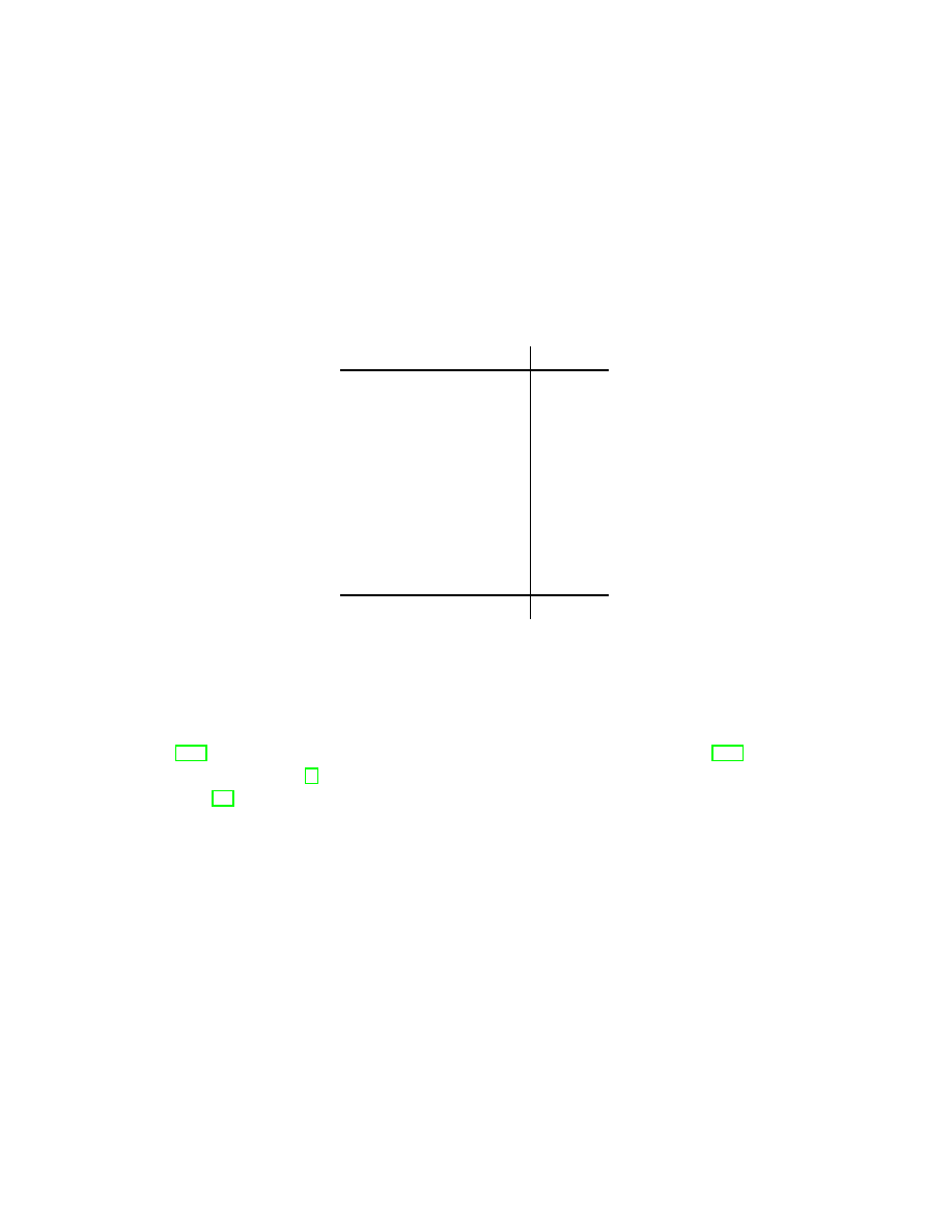
method
-E/a.u.
Thomas-Fermi
625.7
Hartree-Fock
526.818
OEP (exchange only)
526.812
LDA (exchange only)
524.517
LDA (VWN)
525.946
LDA (PW92)
525.940
LDA-SIC(PZ)
528.393
ADA
527.322
WDA
528.957
GGA (B88LYP)
527.551
experiment
527.6
Table 1: Ground-state energy in atomic units (1 a.u. = 1 Hartree = 2
Rydberg = 27.21eV ˆ
=627.5kcal/mol) of the Ar atom (Z = 18), obtained with
some representative density functionals and related methods. The Hartree-
Fock and OEP(exchange only) values are from Krieger et al. (third of Ref.
[120]), ADA and WDA values are from Gunnarsson et al., Ref. [129], as
reported in Ref. [5], and the LDA-SIC(PZ) value is from Perdew and Zunger,
Ref. [93]. The experimental value is based on Veillard and Clementi, J. Chem.
Phys. 49, 2415 (1968), and given to less significant digits than the calculated
values, because of relativistic and quantum electrodynamical effects (Lamb
shift) that are automatically included in the experimental result but not in
the calculated values.
48

5.3
Orbital functionals and other nonlocal approxima-
tions: hybrids, Meta-GGA, SIC, OEP, etc.
In spite of these advances, the quest for more accurate functionals goes ever
on, and both in chemistry and physics various beyond-GGA functionals have
appeared. Perhaps the most popular functional in quantum chemistry
is
B3LYP. This is a combination of the LYP GGA for correlation [98] with
Becke’s three-parameter hybrid functional B3 for exchange [108]. Common
hybrid functionals, such as B3, mix a fraction of Hartree-Fock exchange into
the DFT exchange functional (other mixtures are also possible). The con-
struction of hybrid functional involves a certain amount of empiricism in the
choice of functionals that are mixed and in the optimization of the weight
factors given to the HF and DFT terms. Formally, this might be considered a
drawback, but in practice B3 has proven to be the most successful exchange
functional for chemical applications, in particular when combined with the
LYP GGA functional for E
c
. More extreme examples of this semiempirical
mode of construction of functionals are Becke’s 1997 hybrid functional [109],
which contains 10 adjustable parameters, and the functionals of Refs. [110]
and [111], each of which contains 21 parameters.
Another recent beyond-GGA development is the emergence of so-called
Meta-GGAs, which depend, in addition to the density and its derivatives,
also on the Kohn-Sham kinetic-energy density τ (r) [2, 112, 113]
τ (r) =
¯h
2
2m
X
i
|∇φ
i
(r)|
2
,
(89)
so that E
xc
can be written as E
xc
[n(r), ∇n(r), τ (r)]. The additional degree
of freedom provided by τ is used to satisfy additional constraints on E
xc
,
such as a self-interaction-corrected correlation functional, recovery of the
fourth-order gradient expansion for exchange in the limit of slowly varying
densities, and a finite exchange potential at the nucleus [2]. In several recent
tests [2, 100, 114, 115, 116] Meta-GGAs have given favorable results, even
when compared to the best GGAs, but the full potential of this type of
approximation is only beginning to be explored systematically.
As we have seen in the case of T
s
, it can be much easier to represent a
functional in terms of single-particle orbitals than directly in terms of the
51
This was written in early 2002, but at the time of revision of this text in 2006 it is
still correct.
49
density. Such functionals are known as orbital functionals, and Eq. (54) con-
stitutes a simple example. Another important orbital-dependent functional
is the exchange energy (Fock term) of Eq. (56). The Meta-GGAs and hybrid
functionals mentioned above are also orbital functionals, because they de-
pend on the kinetic energy density (89), and on a combination of the orbital
functional (56) with ordinary GGAs, respectively.
Still another type of orbital functional is the self-interaction correction
(SIC). Most implementations of SIC make use of the expressions proposed
in Ref. [93] (PZ-SIC),
E
approx,SIC
xc
[n
↑
, n
↓
] = E
approx
xc
[n
↑
, n
↓
] −
X
i,σ
(E
H
[n
iσ
] − E
approx
xc
[n
iσ
, 0]) ,
(90)
which subtracts, orbital by orbital, the contribution the Hartree and the xc
functionals would make if there was only one electron in the system. This
correction can be applied on top of any approximate density functional, and
ensures that the resulting corrected functional satisfies E
approx,SIC
xc
[n
(1)
, 0] =
−E
H
[n
(1)
] for a one-electron system. The LDA is exact for a completely
uniform system, and thus is self-interaction free in this limit, but neither it
nor common GGAs satisfy the requirement of freedom from self-interaction
in general, and even Meta-GGAs have a remaining self-interaction error in
their exchange part [2, 112]. This self-interaction is particularly critical for
localized states, such as the d states in transition-metal oxides. For such
systems PZ-SIC has been shown to greatly improve the uncorrected LDA
[71, 72], but for thermochemistry PZ-SIC does not seem to be significant
[117].
Unfortunately the PZ-SIC approach, which minimizes the corrected en-
ergy functional with respect to the orbitals, does not lead to Kohn-Sham
equations of the usual form, because the resulting effective potential is dif-
ferent for each orbital. As a consequence, various specialized algorithms for
minimizing the PZ-SIC energy functional have been developed. For more
details on these algorithms and some interesting applications in solid-state
physics see Refs. [71, 72, 73]. For finite systems, PZ-SIC has also been im-
plemented by means of the OEP [64, 74], which produces a common local
potential for all orbitals, and is discussed in the next paragraph. A detailed
review of implementations and applications of PZ-SIC can be found in the
contribution of Temmerman et al. in Ref. [17]. Alternatives to the PZ-SIC
formulation of Ref. [93] have recently been analysed in [118, 119], with a
view on either improving results obtained with PZ-SIC, or simplifying the
50
implementation of the correction.
Since hybrid functionals, Meta-GGAs, SIC, the Fock term and all other
orbital functionals depend on the density only implicitly, via the orbitals
φ
i
[n], it is not possible to directly calculate the functional derivative v
xc
=
δE
xc
/δn. Instead one must use indirect approaches to minimize E[n] and
obtain v
xc
. In the case of the kinetic-energy functional T
s
[{φ
i
[n]}] this in-
direct approach is simply the Kohn-Sham scheme, described in Sec. 4. In
the case of orbital expressions for E
xc
the corresponding indirect scheme is
known as the optimized effective potential (OEP) [120] or, equivalently, the
optimized-potential model (OPM) [121]. The minimization of the orbital
functional with respect to the density is achieved by repeated application of
the chain rule for functional derivatives,
v
xc
[n](r) =
δE
orb
xc
[{φ
i
}]
δn(r)
=
Z
d
3
r
′
Z
d
3
r
′′
X
i
"
δE
orb
xc
[{φ
i
}]
δφ
i
(r
′
)
δφ
i
(r
′
)
δv
s
(r
′′
)
δv
s
(r
′′
)
δn(r)
+ c.c.
#
,
(91)
where E
orb
xc
is the orbital functional (e.g., the Fock term) and v
s
the KS
effective potential. Further evaluation of Eq. (91) gives rise to an integral
equation that determines the v
xc
[n] belonging to the chosen orbital func-
tional E
xc
[{φ
i
[n]}] [120, 122]. As an alternative to solving the full OEP
integral equation, Krieger, Li and Iafrate (KLI) have proposed a simple but
surprisingly accurate approximation that greatly facilitates implementation
of the OEP [120].
The application of the OEP methodology to the Fock term (56), either
with or without the KLI approximation, is also known as the exact-exchange
method (EXX). The OEP-EXX equations have been solved for atoms [120,
121, 123] and solids [124, 125], with very encouraging results. Other orbital-
dependent functionals that have been treated within the OEP scheme are
the PZ self-interaction correction [64, 74] and the Colle-Salvetti functional
[123]. A detailed review of the OEP and its KLI approximation is Ref. [122].
The high accuracy attained by complex orbital functionals implemented
via the OEP, and the fact that it is easier to devise orbital functionals than
explicit density functionals, makes the OEP concept attractive, but the com-
putational cost of solving the OEP integral equation is a major drawback.
However, this computational cost is significantly reduced by the KLI approx-
imation [120] and other recently proposed simplifications [126, 127, 128]. In
the context of the EXX method (i.e., using the Fock exchange term as orbital
functional) the OEP is a viable way to proceed. For more complex orbital
51
functionals, additional simplifications may be necessary [120, 126, 127, 128].
A further reduction of computational complexity is achieved by not eval-
uating the orbital functional self-consistently, via Eq. (91), but only once,
using the orbitals and densities of a converged self-consistent LDA or GGA
calculation. This ‘post-GGA’ or ‘post-LDA’ strategy completely avoids the
OEP and has been used both for hybrid functionals and Meta-GGAs [108,
109, 112, 113]. A drawback of post methods is that they provide only ap-
proximations to the selfconsistent total energies, not to eigenvalues, effective
potentials, orbitals or densities.
In the case of hybrid functionals, still another mode of implementation has
become popular. This alternative, which also avoids solution of Eq. (91), is
to calculate the derivative of the hybrid functional with respect to the single-
particle orbitals, and not with respect to the density as in (91). The resulting
single-particle equation is of Hartree-Fock form, with a nonlocal potential,
and with a weight factor in front of the Fock term. Strictly speaking, the
orbital derivative is not what the HK theorem demands, but rather a Hartree-
Fock like procedure, but in practice it is a convenient and successful approach.
This scheme, in which self-consistency is obtained with respect to the single-
particle orbitals, can be considered an evolution of the Hartree-Fock Kohn-
Sham method [6], and is how hybrids are commonly implemented. Recently,
it has also been used for Meta-GGAs [2]. For occupied orbitals, results
obtained from orbital selfconsistency differ little from those obtained from
the OEP.
Apart from orbital functionals, which are implicit nonlocal density func-
tionals because the orbitals depend on the density in a nonlocal way, there
is also a class of explicit nonlocal density functionals. Such nonlocal density
functionals take into account, at any point r, not only the density at that
point, n(r), and its derivatives, ∇n(r) etc., but also the behaviour of the
density at different points r
′
6= r, by means of integration over physically
relevant regions of space. A typical example is
E
ADA
xc
[n] =
Z
d
3
r n(r)ǫ
hom
xc
(¯
n(r)),
(92)
where ǫ
hom
xc
is the per-particle xc energy of the homogeneous electron liquid
(see footnote 47). In the LDA one would have ¯
n(r) ≡ n(r), but in the
average-density approximation (ADA) one takes [129]
¯
n(r) =
Z
d
3
r
′
n(r
′
)w[n](|r − r
′
|),
(93)
52
where w[n](|r − r
′
|) is a weight function that samples the density not only
semilocally, as do the GGAs, but over a volume determined by the range of
w. Conceptually similar to the ADA is the weighted-density approximation
(WDA) [129]. In terms of the pair-correlation function (see Secs. 3.5.2 and
4.1.2) the LDA, ADA and WDA functionals can be written as
E
LDA
xc
[n] =
e
2
2
Z
d
3
r
Z
d
3
r
′
n(r)n(r)
|r − r
′
|
(¯
g
hom
[n(r)](r − r
′
) − 1)
(94)
E
ADA
xc
[n] =
e
2
2
Z
d
3
r
Z
d
3
r
′
n(r)¯
n(r)
|r − r
′
|
(¯
g
hom
[¯
n(r)](r − r
′
) − 1)
(95)
E
W DA
xc
[n] =
e
2
2
Z
d
3
r
Z
d
3
r
′
n(r)n(r
′
)
|r − r
′
|
(¯
g
hom
[¯
n(r)](r − r
′
) − 1) ,
(96)
where in each case ¯
g
hom
(r − r
′
) is the pair-correlation function of the homo-
geneous electron liquid, averaged over the coupling constant e
2
The dependence of these functionals on ¯
n(r), the integral over n(r), in-
stead of on derivatives, as in the GGAs, is the reason why such functionals
are called nonlocal. In practice, this integral turns the functionals compu-
tationally expensive, and in spite of their great promise they are much less
used than GGAs. However, recent comparisons of ADA and WDA with LDA
and GGAs for low-dimensional systems [114, 130] and for bulk silicon [131]
show that nonlocal integral-dependent density functionals can outperform
local and semilocal approximations.
6
Extensions of DFT: New frontiers and old
problems
Up to this point we have discussed DFT in terms of the charge (or par-
ticle) density n(r) as fundamental variable. In order to reproduce the cor-
rect charge density of the interacting system in the noninteracting (Kohn-
Sham) system, one must apply to the latter the effective KS potential v
s
=
v + v
H
+ v
xc
, in which the last two terms simulate the effect of the electron-
electron interaction on the charge density. This form of DFT, which is the
one proposed originally [24], could also be called ‘charge-only’ DFT. It is not
the most widely used DFT in practical applications. Much more common
is a formulation that employs one density for each spin, n
↑
(r) and n
↓
(r),
53
i.e, works with two fundamental variables. In order to reproduce both of
these in the noninteracting system one must now apply two effective poten-
tials, v
s,↑
(r) and v
s,↓
(r).
This formulation of DFT is known as spin-DFT
(SDFT) [89, 90]. Its fundamental variables n
↑
(r) and n
↓
(r) can be used to
calculate the charge density n(r) and the spin-magnetization density m(r)
from
n(r) = n
↑
(r) + n
↓
(r)
(97)
m(r) = µ
0
(n
↑
(r) − n
↓
(r)),
(98)
where µ
0
= q¯h/2mc is the Bohr magneton. More generally, the Hohenberg-
Kohn theorem of SDFT states that in the presence of a magnetic field
B(r) that couples only to the electron spin [via the familiar Zeeman term
R
d
3
r m(r)B(r)] the ground-state wave function and all ground-state observ-
ables are unique functionals of n and m or, equivalently, of n
↑
and n
↓
Almost the entire further development of the HK theorem and the KS equa-
tions can be immediately rephrased for SDFT, just by attaching a suitable
spin index to the densities. For this reason we could afford the luxury of
exclusively discussing ‘charge-only’ DFT in the preceding sections, without
missing any essential aspects of SDFT.
There are, however, some exceptions to this simple rule. One is the
fourth statement of the HK theorem, as discussed in Sec. 3.2. Another is the
construction of functionals. For the exchange energy it is known, e.g., that
[132]
E
SDF T
x
[n
↑
, n
↓
] =
1
2
E
DF T
x
[2n
↑
] + E
DF T
x
[2n
↓
]
.
(99)
In analogy to the coordinate scaling of Eqs. (59) - (61), this property is of-
ten called ‘spin-scaling’, and it can be used to construct an SDFT exchange
functional from a given DFT exchange functional. In the context of the
LSDA, von Barth and Hedin [89] wrote the exchange functional in terms
of an interpolation between the unpolarized and fully polarized electron gas
which by construction satisfies Eq. (99). Alternative interpolation procedures
52
More generally, one requires one effective potential for each density-like quantity to
be reproduced in the KS system. Such potentials and corresponding densities are called
conjugate variables.
53
In the particular case B = 0 the SDFT HK theorem still holds and continues to be
useful, e.g., for systems with spontaneous polarization. In principle one could also use
‘charge-only’ DFT to study such systems, but then n
↑
(r) and n
↓
(r) become functionals of
n(r) and nobody knows how to determine these functionals.
54
can be found in Ref. [92]. GGA exchange functionals also satisfy Eq. (99)
by construction. For the correlation energy no scaling relation of the type
(99) holds, so that in practice correlation functionals are either directly con-
structed in terms of the spin densities or written by using, without formal
justification, the same interpolation already used in the exchange functional.
In the case of the LSDA this latter procedure was introduced in Ref. [89],
and further analysed and improved in Ref. [92].
The Kohn-Sham equations of SDFT are
"
−
¯h
2
∇
2
2m
+ v
sσ
(r)
#
φ
iσ
(r) = ǫ
iσ
φ
iσ
(r),
(100)
where v
sσ
(r) = v
σ
(r) + v
H
(r) + v
xc,σ
(r). In a nonrelativistic calculation the
Hartree term does not depend on the spin label,
but in the presence of
an externally applied magnetic field v
σ
(r) = v(r) − σµ
0
B (where σ = ±1).
Finally,
v
xc,σ
(r) =
δE
SDF T
xc
[n
↑
, n
↓
]
δn
σ
(r)
.
(101)
In the presence of an internal magnetic field B
xc
(i.e., in spin-polarized sys-
tems) v
xc,↓
− v
xc,↑
= µ
0
B
xc
. This field is the origin of, e.g., ferromagnetism
in transition metals. References to recent work with SDFT include almost
all practical DFT calculation: SDFT is by far the most widely used form
of DFT.
Some recent work on SDFT is described in Ref. [133]. A more
detailed discussion of SDFT can be found in Refs. [5, 6, 90], and a particu-
larly clear exposition of the construction of xc functionals for SDFT is the
contribution of Kurth and Perdew in Refs. [15, 16].
If the direction of the spins is not uniform in space
one requires a for-
mulation of SDFT in which the spin magnetization is not a scalar, as above,
but a three-component vector m(r). Different proposals for extending SDFT
to this situation are available [134, 135, 136]. One mechanism that can give
rise to noncollinear magnetism is spin-orbit coupling. This is another rela-
tivistic effect [28], and as such it is not consistently treated in either DFT
54
Spin-spin dipolar interactions are a relativistic effect of order (1/c)
2
, as are current-
current interactions.
55
SDFT has become synonymous with DFT to such an extent that often no distinction
is made between the two, i.e., a calculation referred to as a DFT one is most of the time
really an SDFT one.
56
Such ‘noncollinear magnetism’ appears, e.g., as canted or helical spin configurations
in rare-earth compounds, or as domain walls in ferromagnets.
55
or SDFT. A generalization of DFT that does account for spin-orbit coupling
and other relativistic effects is relativistic DFT (RDFT) [137, 138]. Here the
fundamental variable is the relativistic four-component current j
µ
. RDFT
requires a more drastic reformulation of DFT than does SDFT. In particu-
lar, the KS equation of RDFT is now of the form of the single-particle Dirac
equation, instead of the Schr¨odinger equation. There are also many subtle
questions involving renormalizability and the use of the variational princi-
ple in the presence of negative energy states. For details on these problems
and their eventual solution the reader is referred to the chapters by Engel
et al.
in Refs. [10] and [19], and to the book by Eschrig [18]. A didactical
exposition of RDFT, together with representative applications in atomic and
condensed-matter physics, can be found in the book by Strange [28], and a
recent numerical implementation is presented in Ref. [139].
To study the magnetic properties of matter one would often like to be able
to obtain information on the currents in the system and their coupling to pos-
sible external magnetic fields. Important classes of experiments for which this
information is relevant are nuclear magnetic resonance and the quantum Hall
effects. SDFT does not provide explicit information on the currents. RDFT
in principle does, but standard implementations of it are formulated in a
spin-only version, which prohibits extraction of information on the currents.
Furthermore, the formalism of RDFT is considerably more complicated than
that of SDFT. In this situation the formulation of nonrelativistic current-
DFT (CDFT), accomplished by Vignale and Rasolt [140, 141], was a major
step forward. CDFT is formulated explicitly in terms of the (spin) density
and the nonrelativistic paramagnetic current density vector j
p
(r). Some re-
cent applications of CDFT are Refs. [142, 143, 144, 145]. E. K. U. Gross and
the author have shown that the existence of spin currents implies the exis-
tence of a link between the xc functionals of SDFT and those of CDFT [146].
Conceptually, this link is similar to the one of Eq. (99) between functionals
of DFT and SDFT, but the details are quite different. Some approximations
for xc functionals of CDFT are discussed in Refs. [146, 147, 148].
In addition to SDFT, RDFT and CDFT, there exist many other gener-
alizations of DFT that were designed for one or other special purpose. As
examples we mention superconductivity [149, 150, 151, 152] and spin-density
waves [136, 153], but there are many more [5-19]. For reasons of space we
cannot discuss these extensions here. Instead, let us take a brief look at a
problem that requires more radical departures from the framework of con-
ventional DFT: excited states. DFT is formulated in terms of ground-state
56
densities, and it is not immediately obvious how one could extract informa-
tion on excited states from them (although at least in the case of ‘charge-only’
DFT the fourth substatement of the HK theorem guarantees that this must
be possible).
Apart from the ad hoc identification of the KS eigenvalues with true exci-
tation energies, there exists a considerable variety of more sound approaches
to excited states in DFT that have met with some success. The early sug-
gestion of Gunnarsson and Lundqvist [90] to use a symmetry-dependent xc
functional to calculate the lowest-energy excited state of each symmetry class
has been implemented approximately by von Barth [154], but suffers from
lack of knowledge on the symmetry dependence of the functional. More
recent work on this dependence is Ref. [155]. An alternative approach to
excited states, not restricted to the lowest energy state of a given symmetry,
is ensemble DFT, developed by Theophilou [26] and further elaborated by
Oliveira, Gross and Kohn [156]. In this formalism the functional depends on
the particular choice for the ensemble, and a simple approximation for this
dependence is available [156]. Some applications of this method have been
worked out by Nagy [157].
Other DFT approaches to excited states can be found in Refs. [158], [159],
[160] and [31], but the most widely used method today is time-dependent
DFT (TD-DFT). The time-dependent generalization of the HK theorem, the
Runge-Gross theorem, cannot be proven along the lines of the original HK
theorem, but requires a different approach [51, 161]. For recent reviews of
TD-DFT see Ref. [162]. Excited states have first been extracted from TD-
DFT in Refs. [163, 164]. This approach is now implemented in standard
quantum-chemical DFT program packages [165, 166] and is increasingly ap-
plied also in solid-state physics [70]. Another important application of TD-
DFT is to systems in external time-dependent fields, such as atoms in strong
laser fields [167, 168]. First steps towards studying dynamical magnetic phe-
nomena with TD-SDFT have been taken very recently [169].
All these extensions of DFT to time-dependent, magnetic, relativistic and
a multitude of other situations involve more complicated Hamiltonians than
the basic ab initio many-electron Hamiltonian defined by Eqs. (2) to (6).
Instead of attempting to achieve a more complete description of the many-
body system under study by adding additional terms to the Hamiltonian,
it is often advantageous to employ the opposite strategy, and reduce the
complexity of the ab initio Hamiltonian by replacing it by simpler models,
which focalize on specific aspects of the full many-body problem. Density-
57

functional theory can be applied to such model Hamiltonians, too, once a
suitable density-like quantity has been identified as basic variable. Following
pioneering work by Gunnarsson and Sch¨onhammer [170], LDA-type approx-
imations have, e.g., recently been formulated and exploited for the Hubbard
[171], the delta-interaction [172] and the Heisenberg [173] models. Common
aspects and potential uses of DFT for model Hamiltonians are described in
[174].
Still another way of using DFT, which does not depend directly on ap-
proximate solution of Kohn-Sham equations, is the quantification and clari-
fication of traditional chemical concepts, such as electronegativity [6], hard-
ness, softness, Fukui functions, and other reactivity indices [6, 175], or aro-
maticity [176]. The true potential of DFT for this kind of investigation is
only beginning to be explored, but holds much promise.
All extensions of DFT face the same formal questions (e.g., simultaneous
interacting and noninteracting v-representability of the densities, nonunique-
ness of the KS potentials, meaning of the KS eigenvalues) and practical
problems (e.g., how to efficiently solve the KS equations, how to construct
accurate approximations to E
xc
, how to treat systems with very strong cor-
relations) as do the more widely used formulations ‘charge-only’ DFT and
SDFT. These questions and problems, however, have never stopped DFT
from advancing, and at present DFT emerges as the method of choice for
solving a wide variety of quantum mechanical problems in chemistry and
physics — and in many situations, such as large and inhomogeneous sys-
tems, it is the only applicable first-principles method at all.
The future of DFT is bright [3, 61, 177] — but to be able to contribute
to it, the reader must now leave the present superficial overview behind, and
turn to the more advanced treatments available in the literature [5-19].
Acknowledgments The author has learned density-functional theory
from E. K. U. Gross, and then practiced it in collaborations with B. L. Gy¨orffy,
L. N. Oliveira, and G. Vignale. These scholars are in no way responsible
for the content of this work, but the author’s intellectual debt to them is
enormous. Useful comments by J. Quintanilla, H. J. P. Freire, T. Mar-
casso, E. Orestes, N. A. Lima, N. Argaman, V. L. L´ıbero, V. V. Fran¸ca,
M. Odashima, J. M. Morbec, A. P. F´avaro, A. J. R. da Silva and L. N. Oliveira
on earlier versions of this manuscript are gratefully acknowledged. This work
was supported financially by FAPESP and CNPq.
58

References
[1] Proceedings of the VIII’th Brazilian Summer School on Electronic
Structure
(2002), eds. H. F. Santos, P. Z. Coura, S. O. Dantas and
P. M. V. B. Barone.
[2] J. Tao, J. P. Perdew, V. N. Staroverov and G. E. Scuseria, Phys. Rev.
Lett. 91, 146401 (2003); J. Chem. Phys. 119, 12129 (2003); J. Chem.
Phys. 120, 6898 (2004); Phys. Rev. B 69, 075102 (2004).
[3] W. Kohn, Rev. Mod. Phys. 71, 1253 (1999).
[4] J. A. Pople, Rev. Mod. Phys. 71, 1267 (1999).
[5] R. M. Dreizler and E. K. U. Gross, Density Functional Theory (Springer,
Berlin, 1990).
[6] R. G. Parr and W. Yang, Density-Functional Theory of Atoms and
Molecules
(Oxford University Press, Oxford, 1989).
[7] W. Koch and M. C. Holthausen, A Chemist’s Guide to Density Functional
Theory
(John Wiley & Sons, New York, 2001).
[8] R. O. Jones and O. Gunnarsson, Rev. Mod. Phys. 61, 689 (1989).
[9] J. M. Seminario (Ed.), Recent Developments and Applications of Modern
DFT
(Elsevier, Amsterdam, 1996).
[10] R. F. Nalewajski (Ed.), Density Functional Theory I -IV (Springer, Top-
ics in Current Chemistry Vols. 180-183, 1996).
[11] V. I. Anisimov (Ed.), Strong Coulomb Correlations in Electronic Struc-
ture Calculations: Beyond the Local Density Approximation
(Gordon &
Breach, 1999).
[12] N. H. March, Electron Density Theory of Atoms and Molecules (Aca-
demic Press, London, 1992).
[13] B. B. Laird, R. B. Ross and T. Ziegler (Eds.), Chemical Applications of
Density Functional Theory
, (American Chemical Society, 1996).
[14] D. P. Chong (Ed.), Recent Advances in Density Functional Methods
(Singapore, World Scientific, 1995).
59

[15] D. Joulbert (Ed.), Density Functionals:
Theory and Applications
(Springer Lecture Notes in Physics Vol. 500, 1998)
[16] C. Fiolhais, F. Nogueira and M. Marques (Eds.), A Primer in Density
Functional Theory
(Springer Lecture Notes in Physics Vol. 620, 2003).
[17] J. F. Dobson, G. Vignale and M. P. Das (Eds.), Density Functional
Theory: Recent Progress and New Directions
(Plenum, New York, 1998).
[18] H. Eschrig, The Fundamentals of Density Functional Theory (Teubner,
Leipzig, 1996).
[19] E. K. U. Gross and R. M. Dreizler (Eds.), Density Functional Theory
(Plenum, New York, 1995).
[20] N. Argaman and G. Makov, Am. J. Phys. 68, 69 (2000).
[21] E. N. Economou, Green’s Functions in Quantum Physics (Springer, New
York, 1979).
[22] M. Levy, Phys. Rev. A 26, 1200 (1982).
[23] E. H. Lieb in Density Functional Methods in Physics, edited by
R. M. Dreizler and J. da Providencia, (Plenum, New York, 1985).
[24] P. Hohenberg and W. Kohn, Phys. Rev. 136, B864 (1964).
[25] E. Schr¨odinger, Ann. Physik 79, 361, 489, 734 (1926); 80, 437 (1926);
81, 109 (1926).
[26] A. K. Theophilou, J. Phys. C 12, 5419 (1979).
[27] O. Gritsenko and E. J. Baerends, J. Chem. Phys. 120, 8364 (2004).
[28] P. Strange, Relativistic Quantum Mechanics with Applications in Con-
densed Matter and Atomic Physics
(Cambridge University Press, Cam-
bridge, 1998).
[29] T. Kato, Commun. Pure Appl. Math. 10, 151 (1957).
[30] N. H. March, Self-consistent fields in atoms (Pergamon Press, Oxford,
1975).
60

[31] J. P. Perdew and M. Levy, Phys. Rev. B 31, 6264 (1985).
[32] H. Eschrig and W. E. Pickett, Solid State Commun. 118, 123 (2001).
[33] K. Capelle and G. Vignale, Phys. Rev. Lett. 86, 5546 (2001).
[34] K. Capelle and G. Vignale, Phys. Rev. B 65, 113106 (2002).
[35] N. Argaman and G. Makov, Phys. Rev. B 66, 052413 (2002).
[36] N. Gidopolous in The fundamentals of density matrix and density func-
tional theory in atoms, molecules and solids
, N. Gidopoulos and S. Wilson
eds. (Kluwer Series ‘Progress in Theoretical Chemistry and Physics’, 2003);
and cond-mat/0510199.
[37] W. Kohn, A. Savin and C. A. Ullrich, Int. J. Quantum Chem. 100, 20
(2004).
[38] C. A. Ullrich, Phys. Rev. B 72, 073102 (2005).
[39] T. L. Gilbert, Phys. Rev. B 12, 2111 (1975).
[40] J. E. Harriman, Phys. Rev. A 24, 680 (1981).
[41] J. T. Chayes, L. Chayes and M. B. Ruskai, J. Stat. Phys. 38, 497 (1985).
[42] C. A. Ullrich and W. Kohn, Phys. Rev. Lett. 89, 156401 (2002); ibid
87, 093001 (2001).
[43] P. E. Lammert, J. Chem. Phys. 125, 074114 (2006).
[44] A. P. Favaro, J. V. Batista Ferreira and K. Capelle, Phys. Rev. B 73,
045133 (2006).
[45] L. W. Wang and M. P. Teter, Phys. Rev. B 45, 13196 (1992).
[46] M. Foley and P. A. Madden, Phys. Rev. B 53, 10589 (1996).
[47] B. J. Zhou, V. L. Ligneres and E. A. Carter, J. Chem. Phys. 122, 044103
(2005).
[48] E. K. U. Gross, E. Runge and O. Heinonen, Many Particle Theory
(Adam Hilger, 1992).
61

[49] A. Szabo and N. S. Ostlund, Modern Quantum Chemistry (McGraw-
Hill, New York, 1989).
[50] L. J. Sham and M. Schl¨
uter, Phys. Rev. Lett. 51, 1888 (1983).
[51] E. Runge and E. K. U. Gross, Phys. Rev. Lett. 52, 997 (1984).
[52] E. K. U. Gross, M. Petersilka and T. Grabo in Ref. [13].
[53] P. Nozieres and D. Pines, The Theory of Quantum Liquids (Addison
Wesley, New York, revised printing 1989).
[54] N. D. Mermin, Phys. Rev. 137, 1441 (1965).
[55] M. Levy and J. P. Perdew, Phys. Rev. A 32, 2010 (1985).
[56] E. H. Lieb and S. Oxford, Int. J. Quantum Chem. 19, 427 (1981).
[57] G. K.-L. Chan and N. C. Handy, Phys. Rev. A 59, 3075 (1999).
[58] J. P. Perdew, R. G. Parr, M. Levy and J. L. Balduz, Phys. Rev. Lett.
49, 1691 (1982).
[59] J. P. Perdew and M. Levy, Phys. Rev. Lett. 51, 1884 (1983).
[60] W. Kohn and L. J. Sham, Phys. Rev. 140, A1133 (1965).
[61] W. Kohn, A. D. Becke and R. G. Parr, J. Phys. Chem. 100, 12974
(1996).
[62] C. O. Almbladh and U. v. Barth, Phys. Rev. B 31, 3231 (1985).
[63] M. Levy, J. P. Perdew and V. Sahni, Phys. Rev. A 30, 2745 (1984).
[64] J. Chen, J. B. Krieger, Y. Li and G. J. Iafrate, Phys. Rev. A 54, 3939
(1996).
[65] M. L¨
uders, A. Ernst, W. M. Temmerman, Z. Szotek and P. J. Durham,
J. Phys. Cond. Mat. 13, 8587 (2001).
[66] J. Muskat, A. Wander, and N. M. Harrison, Chem. Phys. Lett. 342, 397
(2001).
62

[67] A. Savin, C. J. Umrigar and X. Gonze, Chem. Phys. Lett. 288, 391
(1998).
[68] W. G. Aulbur, L. J¨onsson and J. W. Wilkins, Solid State Phys. 54, 1
(1999).
[69] F. Aryasetiawan and O. Gunnarsson, Rep. Prog. Phys. 61, 237 (1998).
[70] G. Onida, L. Reining and A. Rubio, Rev. Mod. Phys. 74, 601 (2002).
[71] A. Svane and O. Gunnarsson, Phys. Rev. Lett. 65, 1148 (1990); ibid 72,
1248 (1994).
[72] Z. Szotek, W. M. Temmermann and H. Winter, Phys. Rev. Lett. 72,
1244 (1994).
[73] P. Strange, A. Svane, W. M. Temmermann, Z. Szotek and H. Winter,
Nature 399, 756 (1999).
[74] M. R. Norman and D. D. Koelling, Phys. Rev. B 30, 5530 (1984).
[75] O. K. Andersen, Phys. Rev. B 12, 3060 (1975).
[76] O. K. Andersen, O. Jepsen and D. Gl¨otzel in Highlights of Condensed
Matter Theory
, F. Bassani, F. Funi and M. P. Tosi, eds. (North Holland,
Amsterdam, 1985).
[77] O. K. Andersen and T. Saha-Dasgupta, Phys. Rev. B 62, 16219 (2000).
[78] E. Zurek, O. Jepsen and O. K. Andersen, Chem.Phys.Chem. 6, 1934
(2005).
[79] T. H. Dunning Jr., J. Chem. Phys. 90, 1007 (1989).
[80] A. B. F. da Silva, H. F. M. da Costa and M. Trsic, Mol. Phys. 68, 433
(1989).
[81] F. E. Jorge, E. V. R. de Castro and A. B. F. da Silva, J. Comp. Chem.
18, 1565 (1997).
[82] G. B. Bachelet, D. R. Hamann and M. Schl¨
uter, Phys. Rev. B 25, 2103
(1982).
63

[83] L. Kleinman and D. M. Bylander, Phys. Rev. Lett. 48, 1425 (1982).
[84] D. Vanderbilt, Phys. Rev. B 41, 7892 (1990).
[85] N. Troullier and J. L. Martins, Phys. Rev. B 43, 1993 (1991).
[86] W. E. Pickett, Comp. Phys. Rep. 9, 116 (1989).
[87] D. Porezag, M. R. Pederson and A. Y. Liu, Phys. Stat. Sol. (b) 217,
219 (2000)
[88] M. C. Payne, M. P. Teter, D. C. Allan, T. A. Arias and J. D. Joannopou-
los, Rev. Mod. Phys. 64, 1045 (1992).
[89] U. von Barth and L. Hedin, J. Phys. C 5, 1629 (1972).
[90] O. Gunnarsson and B. Lundqvist, Phys. Rev. B 13, 4274 (1976).
[91] D. M. Ceperley and B. J. Alder, Phys. Rev. Lett. 45, 566 (1980).
[92] S. H. Vosko, L. Wilk and M. Nusair, Can. J. Phys. 58, 1200 (1980).
[93] J. P. Perdew and A. Zunger, Phys. Rev. B 23, 5048 (1981).
[94] J. P. Perdew and Y. Wang, Phys. Rev. B 45, 13244 (1992).
[95] J. P. Perdew and Y. Wang, Phys. Rev. B 33, 8800 (1986).
[96] J. P. Perdew, K. Burke and M. Ernzerhof, Phys. Rev. Lett. 77, 3865
(1996); ibid 78, 1396(E) (1997). See also V. Staroverov et al., Phys. Rev.
A 74, 044501 (2006).
[97] A. D. Becke, Phys. Rev. A 38, 3098 (1988).
[98] C. Lee, W. Yang and R. G. Parr, Phys. Rev. B 37, 785 (1988).
[99] D. C. Patton and M. R. Pederson, Phys. Rev. A 56, 2495 (1997).
[100] J. Tao and J. P. Perdew, J. Chem. Phys. 122, 114102 (2005).
[101] W. Kohn, Y. Meir and D. E. Makarov, Phys. Rev. Lett. 80, 4153
(1998).
64

[102] M. Lein, J. F. Dobson and E. K. U. Gross, J. Comp. Chem. 20, 12
(1999).
[103] J. F. Dobson and B. P. Dinte, Phys. Rev. Lett. 76, 1780 (1996).
[104] Y. Andersson, D. C. Langreth and B. I. Lundqvist, Phys. Rev. Lett.
76, 102 (1996).
[105] E. R. Johnson and A. D. Becke, J. Chem. Phys. 123, 024101 (2005).
[106] C. Filippi, C. J. Umrigar and M. Taut, J. Chem. Phys. 100, 1290
(1994).
[107] P. Ziesche, S. Kurth and J. P. Perdew, Comp. Mat. Sci. 11, 122 (1998).
[108] A. D. Becke, J. Chem. Phys. 98, 5648 (1993).
[109] A. D. Becke, J. Chem. Phys. 107, 8554 (1997). See also A. D. Becke,
J. Comp. Chem. 20, 63 (1999).
[110] D. J. Tozer and N. C. Handy, J. Chem. Phys. 108, 2545 (1998).
[111] T. van Voorhis and G. E. Scuseria, J. Chem. Phys. 109, 400 (1998).
[112] J. P. Perdew, S. Kurth, A. Zupan and P. Blaha, Phys. Rev. Lett. 82,
2544 (1999).
[113] A. D. Becke, J. Chem. Phys. 104, 1040 (1996).
[114] Y. H. Ki, I. H. Lee, S. Nagaraja, J. P. Leburton, R. Q. Hood, and
R. M. Martin, Phys. Rev. B 61, 5202 (2000).
[115] S. Kurth, J. P. Perdew and P. Blaha, Int. J. Quantum Chem. 75, 889
(1999).
[116] C. Adamo, M. Ernzerhof and G. E. Scuseria, J. Chem. Phys. 112, 2643
(2000).
[117] O. A. Vydrow and G. E. Scuseria, J. Chem. Phys. 121, 8187 (2004).
[118] U. Lundin and O. Eriksson, Int. J. Quantum. Chem. 81, 247 (2001).
[119] C. Legrand, E. Suraud and P.-G. Reinhard, J. Phys. B 35, 1115 (2002).
65

[120] J. B. Krieger, Y. Li and G. J. Iafrate, Phys. Rev. A 45, 101 (1992);
ibid
46, 5453 (1992); ibid 47 165 (1993).
[121] E. Engel and S. H. Vosko, Phys. Rev. A 47, 2800 (1993).
[122] T. Grabo, T. Kreibich, S. Kurth and E. K. U. Gross, in Ref. [11].
[123] T. Grabo and E. K. U. Gross, Int. J. Quantum Chem. 64, 95 (1997).
T. Grabo and E. K. U. Gross, Chem. Phys. Lett. 240, 141 (1995).
[124] T. Kotani, Phys. Rev. Lett. 74, 2989 (1995).
[125] M. Stadele, J. A. Majewski, P. Vogl and A. G¨orling, Phys. Rev. Lett.
79, 2089 (1997). M. Stadele, M. Moukara, J. A. Majewski, P. Vogl and
A. G¨orling, Phys. Rev. B 59, 10031 (1999). Y.-H. Kim, M. Stadele and
R. M. Martin, Phys. Rev. A 60, 3633 (1999).
[126] S. K¨
ummel and J. P. Perdew, Phys. Rev. B 68, 035103 (2003).
[127] W. Yang and Q. Qu, Phys. Rev. Lett. 89, 143002 (2002).
[128] V. N. Staroverov, G. E. Scuseria and E. R. Davidson, J. Chem. Phys.
125, 081104 (2006).
[129] O. Gunnarsson, M. Jonson and B. I. Lundqvist, Phys. Rev. B 20, 3136
(1979).
[130] A. Cancio, M. Y. Chou and R. O. Hood, Phys. Rev. B 64, 115112
(2002).
[131] P. Garcia-Gonzalez, Phys. Rev. B 62, 2321 (2000).
[132] G. L. Oliver and J. P. Perdew, Phys. Rev. A 20, 397 (1979).
[133] K. Capelle and V. L. Libero, Int. J. Quantum Chem. 105, 679 (2005).
[134] L. M. Sandratskii, Adv. Phys. 47, 91 (1998).
[135] L. Nordstr¨om and D. Singh, Phys. Rev. Lett. 76, 4420 (1996).
[136] K. Capelle and L. N. Oliveira, Phys. Rev. B 61, 15228 (2000).
[137] A. K. Rajagopal and J. Callaway, Phys. Rev. B 7, 1912 (1973).
66

[138] A. H. Mac Donald and S. H. Vosko, J. Phys. C 12, 2977 (1979).
[139] E. Engel, T. Auth and R. M. Dreizler, Phys. Rev. B 64, 235126 (2001).
[140] G. Vignale and M. Rasolt, Phys. Rev. Lett. 59, 2360 (1987).
[141] G. Vignale and M. Rasolt, Phys. Rev. B 37, 10685 (1988).
[142] M. Ferconi and G. Vignale, Phys. Rev. B 50, 14722 (1997).
[143] M. Battocletti, H. Ebert and E. K. U. Gross, Europhys. Lett. 40, 545
(1997).
[144] A. M. Lee, N. C. Handy and S. M. Colwell, J. Chem. Phys. 103, 10095
(1996).
[145] K. Capelle, Phys. Rev. B 65, 100515 (2002).
[146] K. Capelle and E. K. U. Gross, Phys. Rev. Lett. 78, 1872 (1997).
[147] P. Skudlarski and G. Vignale, Phys. Rev. B 48, 8547 (1993).
[148] E. Orestes, T. Marcasso and K. Capelle, Phys. Rev. A 68, 022105
(2003).
[149] L. N. Oliveira, E. K. U. Gross and W. Kohn, Phys. Rev. Lett. 60, 2430
(1988).
[150] W. Kohn, E. K. U. Gross and L. N. Oliveira, J. de Physique 50, 2601
(1989).
[151] W. M. Temmermann, Z. Szotek, B. L. Gyorffy, O. K. Andersen, and
O. Jepsen, Phys. Rev. Lett. 76, 307 (1996).
[152] S. Kurth, M. Marques, M. L¨
uders and E. K. U. Gross, Phys. Rev. Lett.
83, 2628 (1999).
[153] K. Capelle and L. N. Oliveira, Europhys. Lett. 49, 376 (2000).
[154] U. von Barth, Phys. Rev. A 20, 1693 (1979).
[155] A. G¨orling, Phys. Rev. Lett. 85, 4229 (2000).
67

[156] E. K. U. Gross, L. N. Oliveira and W. Kohn, Phys. Rev. A 37, 2805;
ibid
2809; ibid 2821 (1988).
[157] A. Nagy, Phys. Rev. A 49, 3074 (1994); ibid 42, 4388 (1990).
[158] A. G¨orling, Phys. Rev A 59, 3359 (1999). A. G¨orling, Phys. Rev A 54,
3912 (1996).
[159] A. Nagy, Chem. Phys. Lett. 296, 489 (1998). M. Levy and A. Nagy,
Phys. Rev. Lett. 83, 4361 (1999).
[160] K. Capelle, J. Chem. Phys. 119, 1285 (2003).
[161] R. van Leeuwen, Phys. Rev. Lett. 82, 3863 (1999).
[162] E. K. U. Gross, J. F. Dobson and M. Petersilka in Ref. [10]. K. Burke
and E. K. U. Gross in Ref. [15].
[163] M. Petersilka, U. J. Gossmann and E. K. U. Gross, Phys. Rev. Lett.
76, 1212 (1996). See also T. Grabo, M. Petersilka and E. K. U. Gross, J.
Mol. Struc. (Theochem) 501, 353 (2000).
[164] M. E. Casida, in Ref. [14]. J. Jamorski, M. E. Casida and D. R. Salahub,
J. Chem. Phys. 104, 5134 (1996).
[165] S. J. A. van Gisbergen, J. G. Snijders, G. te Velde and E. J. Baerends,
Comp. Phys. Comm. 118, 119 (1999).
[166] R. E. Stratmann, G. E. Scuseria and M. J. Frisch, J. Chem. Phys. 109,
8218 (1998).
[167] M. Lein, E. K. U. Gross and V. Engel, Phys. Rev. Lett. 85, 4707 (2000).
[168] C. A. Ullrich and E. K. U. Gross, Comm. At. Mol. Phys. 33, 211 (1997).
[169] K. Capelle, G. Vignale and B. L. Gyorffy, Phys. Rev. Lett. 87, 206403
(2001). K. Capelle and B. L. Gyorffy, Europhys. Lett. 61, 354 (2003).
[170] O. Gunnarsson and K. Sch¨onhammer, Phys. Rev. Lett. 56, 1968 (1986).
68

[171] N. A. Lima, M. F. Silva, L. N. Oliveira and K. Capelle, Phys. Rev.
Lett. 90, 146402 (2003). N. A. Lima, L. N. Oliveira and K. Capelle, Eu-
rophys. Lett. 60, 601 (2002). M. F. Silva, N. A. Lima, A. L. Malvezzi and
K. Capelle, Phys. Rev. B 71, 125130 (2005). G. Xianlong et al., Phys. Rev.
B 73, 165120 (2006).
[172] R. J. Magyar and K. Burke, Phys. Rev. A 70, 032508 (2004).
[173] V. L. L´ıbero and K. Capelle, Phys. Rev. B 68, 024423 (2003) and Phys.
B 384, 179 (2006). P. E. G. Assis, V. L. Libero and K. Capelle, Phys. Rev.
B 71, 052402 (2005). See also Ref. [133].
[174] V. L. Libero and K. Capelle, cond-mat/0506206.
[175] H. Chermette, J. Comp. Chem. 20, 129 (1999).
[176] F. De Proft and P. Geerlings, Chem. Rev. 101, 1451 (2001).
[177] A. E. Mattsson, Science 298, 759 (2002).
69
Document Outline
- Preface
- What is density-functional theory?
- DFT as a many-body theory
- DFT as an effective single-body theory: The Kohn-Sham equations
- Making DFT practical: Approximations
- Extensions of DFT: New frontiers and old problems
- References
Wyszukiwarka
Podobne podstrony:
mapi com The Ayurvedic View of Marijuana
Candide Voltaire's Opposing View of Optimism in the World
mapi com The Ayurvedic View of Marijuana
David Icke An Other Dimensional View of the American Catastrophe from a Source They Cannot Silence
The Islamic View and the Christian View of
Huckleberry Finn Mark Twain s View of the World doc
George Berkeley His View of God doc
08 Polak M A Preventing punching shear failures of reinforced concrete slabs, results of static and
The Dark Eye Chains of Satinav poradnik do gry
Flannery O Connor A View of the Woods (rtf)(1)
A View of Tuscany
William Sandys Short View of the History of Freemasonry 1829
Buckland, Panagiotakopulu, A paleoecologists view of landnam
Catcher in the Rye, The Holden s View of the Real World doc
Today s View of the Third Reich and the Second World War in German Historiographical Discourse
A comparative view of Englis, Czech, French and Germa idioms
An Epidemiological View of Worms and Viruses
nutritional modulation of immune function
więcej podobnych podstron